introduction to probability and statistics linear regression and correlation
TRANSCRIPT

Introduction to Probability
and Statistics
Linear Regression and Correlation

Example
Let y be a student’s college achievement, measured by his/her GPA. This might be a function of several variables: x1 = rank in high school class x2 = high school’s overall rating x3 = high school GPA x4 = SAT scores
We want to predict y using knowledge of x1, x2, x3 and x4.

Some Questions Which of the independent variables are
useful and which are not? How could we create a prediction equation
to allow us to predict y using knowledge of x1, x2, x3 etc?
How good is this prediction?
We start with the simplest case, in which the response y is a function of a single independent variable, x.
We start with the simplest case, in which the response y is a function of a single independent variable, x.

A Simple Linear Model
We use the equation of a line to describe the relationship between y and x for a sample of n pairs, (x, y).
If we want to describe the relationship between y and x for the whole population, there are two models we can choose
•Deterministic Model: y = x•Probabilistic Model:
–y = deterministic model + random error–y = x
•Deterministic Model: y = x•Probabilistic Model:
–y = deterministic model + random error–y = x
A Simple Linear Model
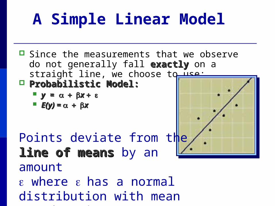
Since the measurements that we observe do not generally fall exactly exactly on a straight line, we choose to use:
Probabilistic Model: Probabilistic Model: yy = = x x E(y) = E(y) = x x
Points deviate from the line of meansline of means by an amount where has a normal distribution with mean 0 and variance 2.
The Random Error
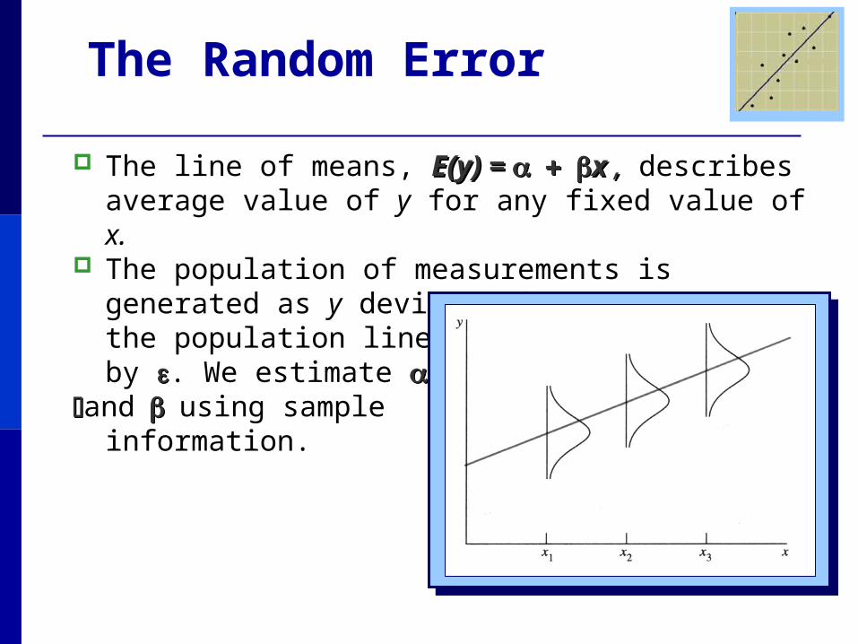
The line of means, E(y) = E(y) = xx , , describes average value of y for any fixed value of x.
The population of measurements is generated as y deviates from the population line by . We estimate
andusing sampleinformation.
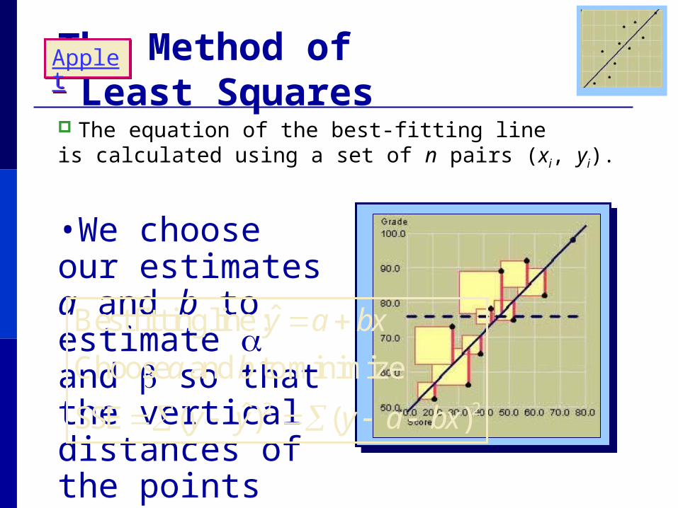
The Method of Least Squares The equation of the best-fitting line is calculated using a set of n pairs (xi, yi).
•We choose our estimates a and b to estimate and so that the vertical distances of the points from the line,are minimized.
22 )()ˆ(
ˆ
bxayyy
ba
bxay
SSE
minimize to and Choose
:line fitting Best
AppletApplet
Least Squares Estimators
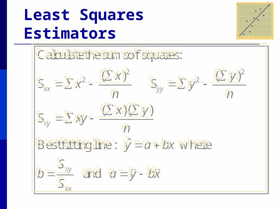
xbyaS
Sb
bxayn
yxxy
n
yy
n
xx
xx
xy
xy
yyxx
and
where :line fitting Best
S
S S
:squares of sums the Calculate
ˆ
))((
)()( 22
22
xbyaS
Sb
bxayn
yxxy
n
yy
n
xx
xx
xy
xy
yyxx
and
where :line fitting Best
S
S S
:squares of sums the Calculate
ˆ
))((
)()( 22
22
Example
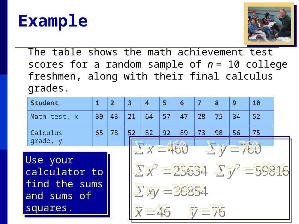
The table shows the math achievement test scores for a random sample of n = 10 college freshmen, along with their final calculus grades.
Student 1 2 3 4 5 6 7 8 9 10
Math test, x 39 43 21 64 57 47 28 75 34 52
Calculus grade, y 65 78 52 82 92 89 73 98 56 75
Use your calculator to find the sums and sums of squares.
Use your calculator to find the sums and sums of squares.
7646
36854
5981623634
76046022
yx
xy
yx
yx
7646
36854
5981623634
76046022
yx
xy
yx
yx
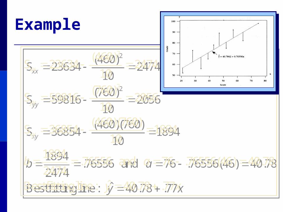
:line fitting Best
and .76556
S
2056S
2474S
xy
ab
xy
yy
xx
77.78.40ˆ
78.40)46(76556.762474
1894
189410
)760)(460(36854
10
)760(59816
10
)460(23634
2
2
:line fitting Best
and .76556
S
2056S
2474S
xy
ab
xy
yy
xx
77.78.40ˆ
78.40)46(76556.762474
1894
189410
)760)(460(36854
10
)760(59816
10
)460(23634
2
2
Example

The total variation in the experiment is measured by the total sum of squarestotal sum of squares:
The Analysis of Variance
2)yyS yy ( SS Total2)yyS yy ( SS Total
The Total SSTotal SS is divided into two parts:
SSRSSR (sum of squares for regression): measures the variation explained by using x in the model.
SSESSE (sum of squares for error): measures the leftover variation not explained by x.

The Analysis of Variance
We calculate
0259.606
9741.14492056
)(
9741.1449
2474
1894)(
2
22
xx
xyyy
xx
xy
S
SS
S
S
SSR - SS TotalSSE
SSR
0259.606
9741.14492056
)(
9741.1449
2474
1894)(
2
22
xx
xyyy
xx
xy
S
SS
S
S
SSR - SS TotalSSE
SSR
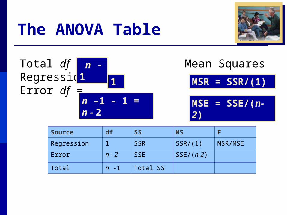
The ANOVA Table
Total df = Mean SquaresRegression df = Error df =
n -1
1
n –1 – 1 = n - 2
MSR = SSR/(1)
MSE = SSE/(n-2)
Source df SS MS F
Regression 1 SSR SSR/(1) MSR/MSE
Error n - 2 SSE SSE/(n-2)
Total n -1 Total SS
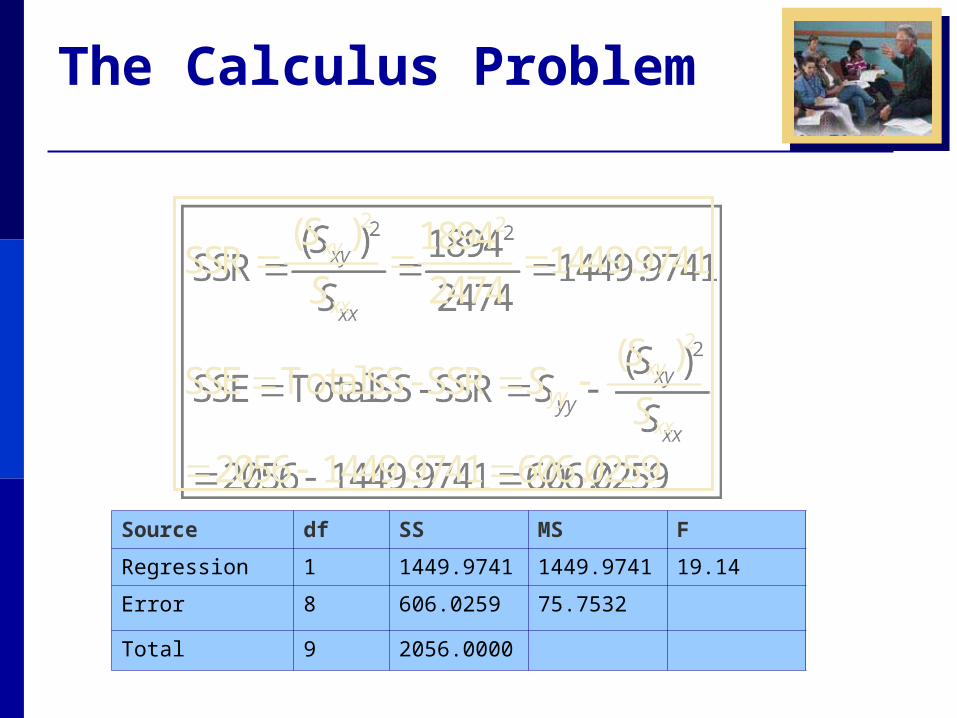
The Calculus Problem
Source df SS MS F
Regression 1 1449.9741 1449.9741 19.14
Error 8 606.0259 75.7532
Total 9 2056.0000
0259.6069741.14492056
)(
9741.14492474
1894)(
2
22
xx
xyyy
xx
xy
S
SS
S
S
SSR - SS TotalSSE
SSR
0259.6069741.14492056
)(
9741.14492474
1894)(
2
22
xx
xyyy
xx
xy
S
SS
S
S
SSR - SS TotalSSE
SSR

Testing the Usefulness of the Model• The first question to ask is whether the
independent variable x is of any use in predicting y.
• If it is not, then the value of y does not change, regardless of the value of x. This implies that the slope of the line, , is zero.
0:0:0 aH versusH 0:0:0 aH versusH
Testing the Usefulness of the Model
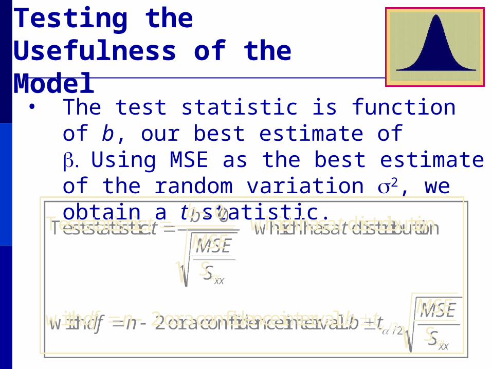
• The test statistic is function of b, our best estimate of Using MSE as the best estimate of the random variation 2, we obtain a t statistic.
xx
xx
S
MSEtbndf
t
S
MSE
bt
2/2
0
:interval confidencea or with
ondistributi a has which :statistic Test
xx
xx
S
MSEtbndf
t
S
MSE
bt
2/2
0
:interval confidencea or with
ondistributi a has which :statistic Test

The Calculus Problem• Is there a significant relationship between the calculus
grades and the test scores at the 5% level of significance?
AppletApplet
38.42474/7532.75
07656.
/
0
xxS
bt
MSE
0:0:0 aH versusH
Reject H 0 when |t| > 2.306. Since t = 4.38 falls into the rejection region, H 0 is rejected .
There is a significant linear relationship between the calculus grades and the test scores for the population of college freshmen.

The F Test
You can test the overall usefulness of the model using an F test. If the model is useful, MSR will be large compared to the unexplained variation, MSE.
predicting in useful is modelH test To 0 y:
. 2- and withFF if H Reject
MSEMSR
F :Statistic Test
0 dfn 1
This test is exactly equivalent to the t-test, with t2 = F.

Measuring the Strength of the Relationship • If the independent variable x is of useful in
predicting y, you will want to know how well the model fits.
• The strength of the relationship between x and y can be measured using:
SS TotalSSR
:iondeterminat of tCoefficien
:tcoefficien nCorrelatio
yyxx
xy
yyxx
xy
SS
Sr
SS
Sr
2
2
SS TotalSSR
:iondeterminat of tCoefficien
:tcoefficien nCorrelatio
yyxx
xy
yyxx
xy
SS
Sr
SS
Sr
2
2

Measuring the Strength of the Relationship • Since Total SS = SSR + SSE, r2 measures the proportion of the total variation in the
responses that can be explained by using the independent variable x in the model.
the percent reduction the total variation by using the regression equation rather than just using the sample mean y-bar to estimate y.
SS TotalSSR
2rSS Total
SSR 2r
For the calculus problem, r2 = .705 or 70.5%. The model is working well!

Interpreting a Significant Regression • Even if you do not reject the null hypothesis
that the slope of the line equals 0, it does not
necessarily mean that y and x are unrelated.
• Type II error—falsely declaring that the slope is
0 and that x and y are unrelated.
• It may happen that y and x are perfectly related
in a nonlinear way.

Some Cautions • You may have fit the wrong model.
•Extrapolation—predicting values of y outside
the range of the fitted data.
•Causality—Do not conclude that x causes y.
There may be an unknown variable at work!
Checking the Regression Assumptions
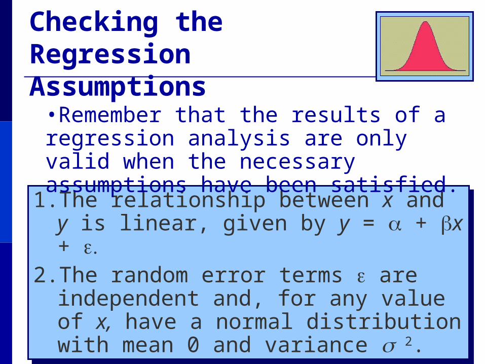
1. The relationship between x and y is linear, given by y = + x +
2. The random error terms are independent and, for any value of x, have a normal distribution with mean 0 and variance 2.
1. The relationship between x and y is linear, given by y = + x +
2. The random error terms are independent and, for any value of x, have a normal distribution with mean 0 and variance 2.
•Remember that the results of a regression analysis are only valid when the necessary assumptions have been satisfied.

Diagnostic Tools
1. Normal probability plot of residuals2. Plot of residuals versus fit or
residuals versus variables
1. Normal probability plot of residuals2. Plot of residuals versus fit or
residuals versus variables
•We use the following diagnostic tools to check the normality assumption and the assumption of equal variances.
Residuals
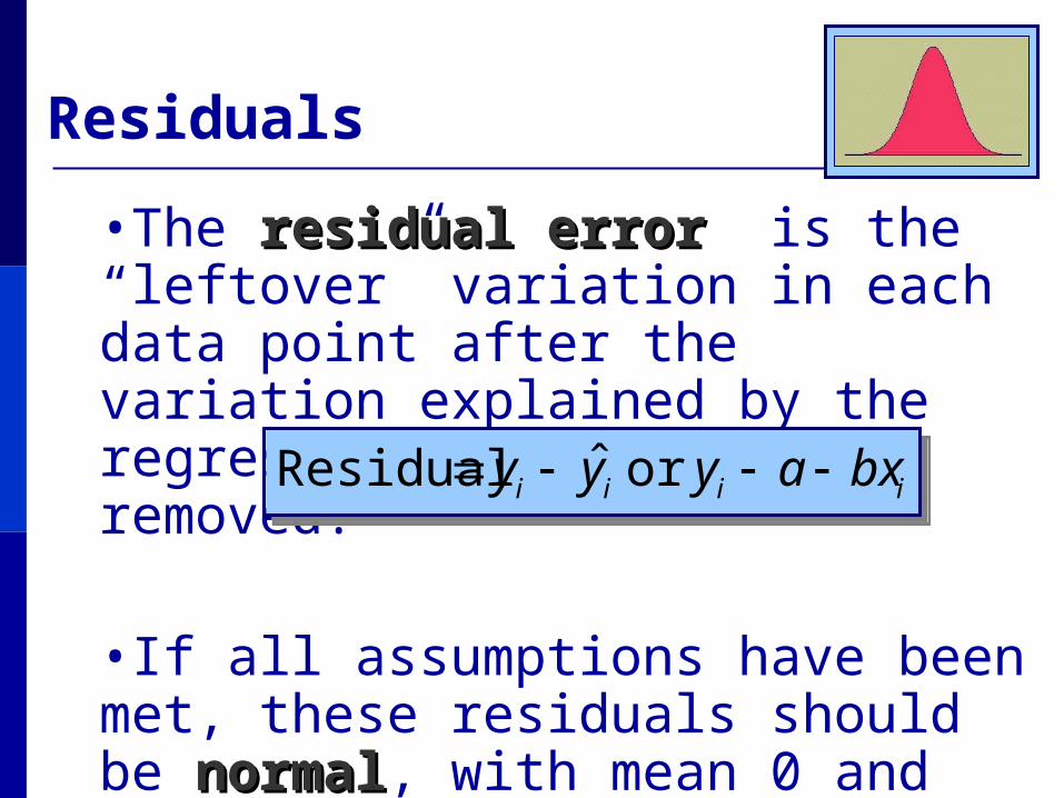
•The residual errorresidual error is the “leftover” variation in each data point after the variation explained by the regression model has been removed.
•If all assumptions have been met, these residuals should be normalnormal, with mean 0 and variance 2.
iiii bxayyy or Residual ˆ iiii bxayyy or Residual ˆ

If the normality assumption is valid, the plot should resemble a straight line, sloping upward to the right.
If not, you will often see the pattern fail in the tails of the graph.
If the normality assumption is valid, the plot should resemble a straight line, sloping upward to the right.
If not, you will often see the pattern fail in the tails of the graph.
Normal Probability Plot
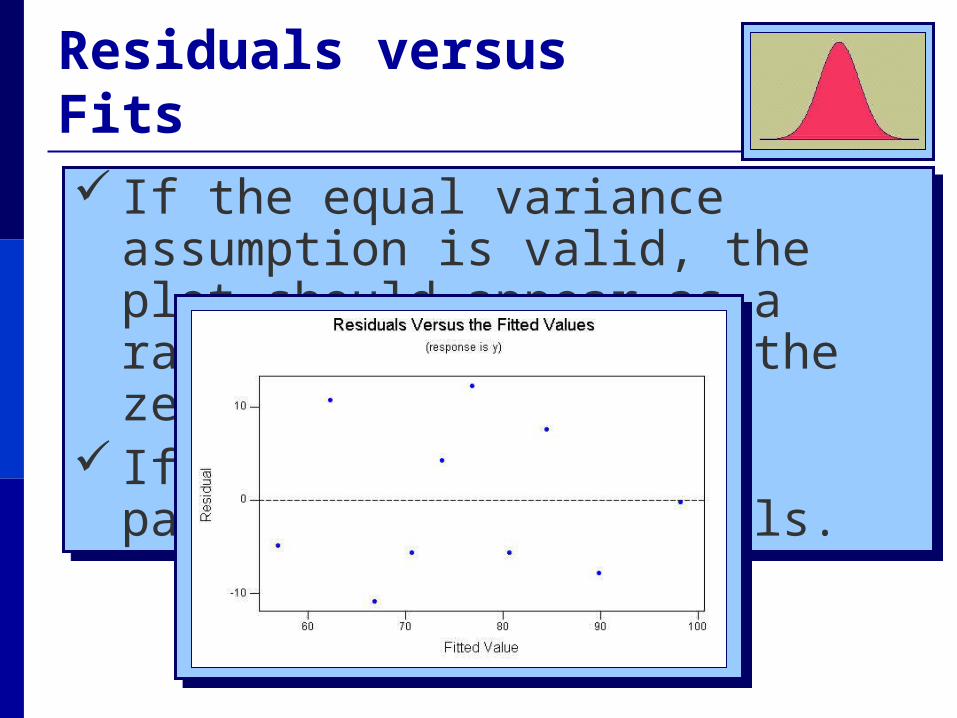
If the equal variance assumption is valid, the plot should appear as a random scatter around the zero center line.
If not, you will see a pattern in the residuals.
If the equal variance assumption is valid, the plot should appear as a random scatter around the zero center line.
If not, you will see a pattern in the residuals.
Residuals versus Fits

Estimation and Prediction
• Once you have determined that the regression line is useful used the diagnostic plots to check for
violation of the regression assumptions.
• You are ready to use the regression line to Estimate the average value of y for a
given value of x Predict a particular value of y for a
given value of x.
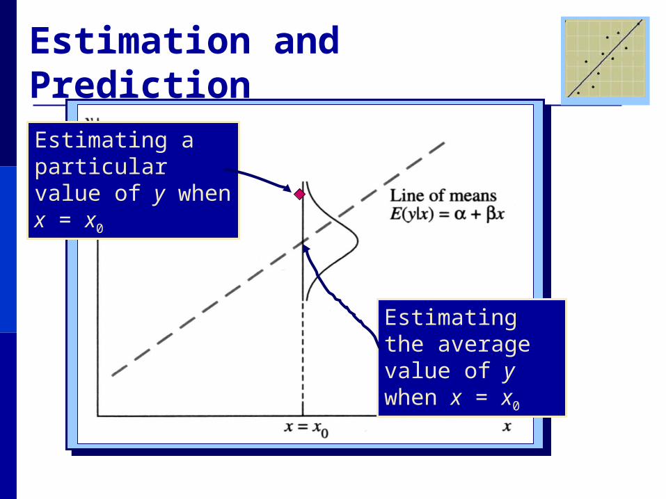
Estimation and Prediction
Estimating the average value of y when x = x0
Estimating a particular value of y when x = x0

Estimation and Prediction • The best estimate of either E(y) or y for a given value x = x0 is
• Particular values of y are more difficult to predict, requiring a wider range of values in the prediction interval.
0ˆ bxay 0ˆ bxay

Estimation and Prediction
xx
xx
S
xx
nMSEty
xxy
S
xx
nMSEty
xxy
20
2/
0
20
2/
0
)(11ˆ
)(1ˆ
: when of valueparticulara predict To
: when of valueaverage the estimate To
xx
xx
S
xx
nMSEty
xxy
S
xx
nMSEty
xxy
20
2/
0
20
2/
0
)(11ˆ
)(1ˆ
: when of valueparticulara predict To
: when of valueaverage the estimate To

The Calculus Problem Estimate the average calculus grade for students
whose achievement score is 50 with a 95% confidence interval.
85.61. to 72.51or
79.06.76556(50)40.78424 Calculate
55.606.79
2474
)4650(
10
17532.75306.2ˆ
ˆ
2
y
y
85.61. to 72.51or
79.06.76556(50)40.78424 Calculate
55.606.79
2474
)4650(
10
17532.75306.2ˆ
ˆ
2
y
y
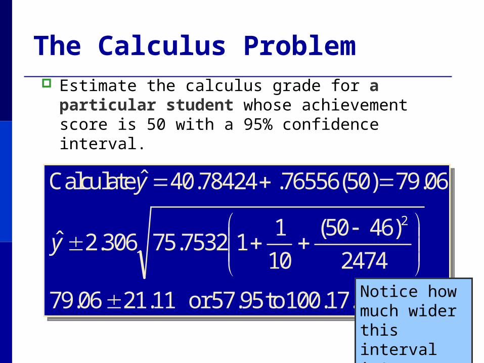
The Calculus Problem Estimate the calculus grade for a particular
student whose achievement score is 50 with a 95% confidence interval.
100.17. to 57.95or
79.06.76556(50)40.78424 Calculate
11.2106.79
2474
)4650(
10
117532.75306.2ˆ
ˆ
2
y
y
100.17. to 57.95or
79.06.76556(50)40.78424 Calculate
11.2106.79
2474
)4650(
10
117532.75306.2ˆ
ˆ
2
y
y
Notice how much wider this interval is!
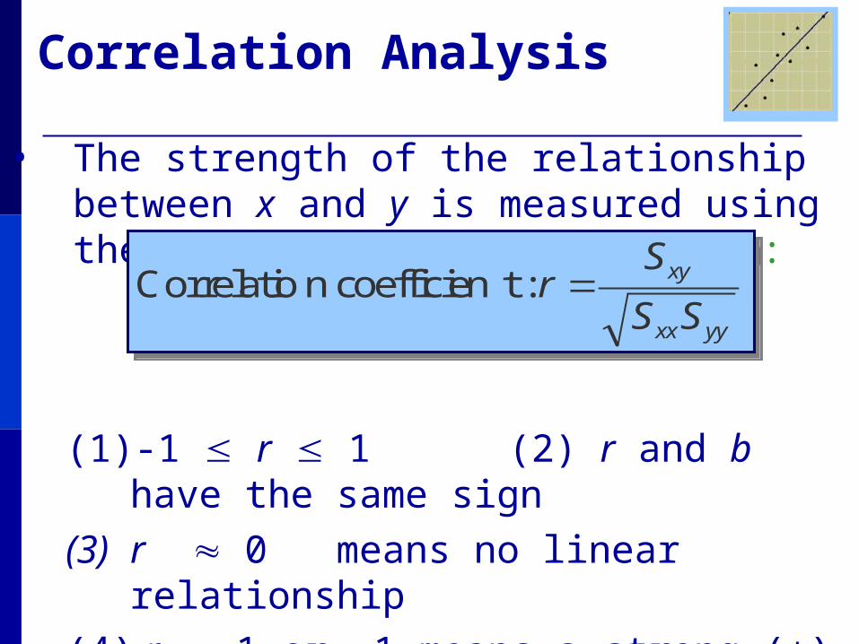
Correlation Analysis
• The strength of the relationship between x and y is measured using the coefficient of correlationcoefficient of correlation:
:tcoefficienn Correlatioyyxx
xy
SS
Sr :tcoefficienn Correlatio
yyxx
xy
SS
Sr
(1) -1 r 1 (2) r and b have the same sign
(3) r 0 means no linear relationship
(4) r 1 or –1 means a strong (+) or (-) relationship
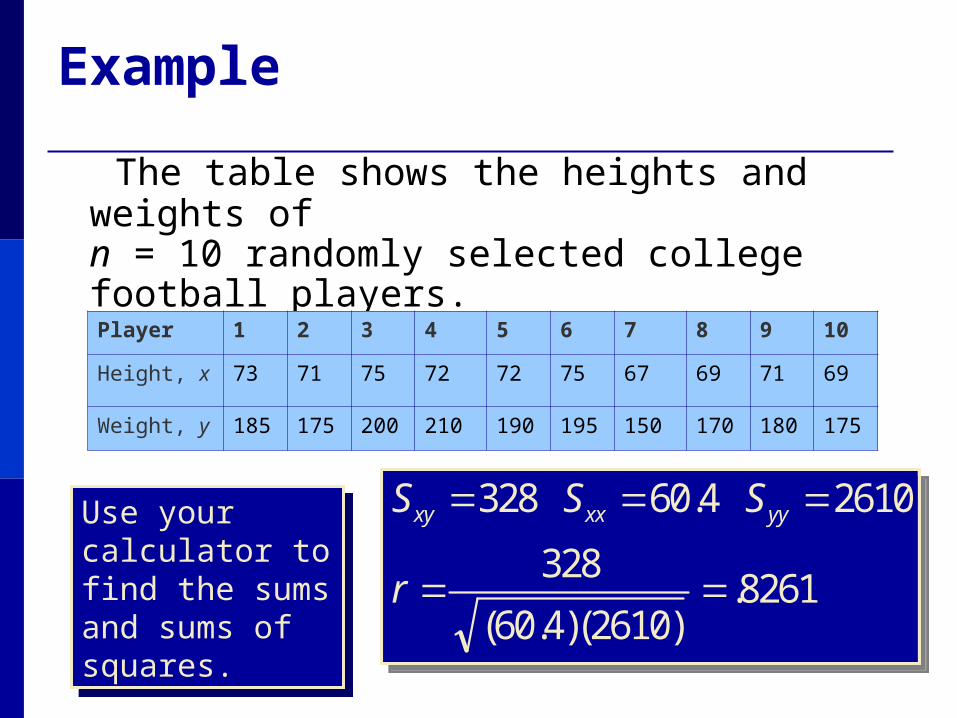
Example
The table shows the heights and weights ofn = 10 randomly selected college football players.
Player 1 2 3 4 5 6 7 8 9 10
Height, x 73 71 75 72 72 75 67 69 71 69
Weight, y 185 175 200 210 190 195 150 170 180 175
Use your calculator to find the sums and sums of squares.
Use your calculator to find the sums and sums of squares.
8261.)2610)(4.60(
328
26104.60328
r
SSS yyxxxy
8261.)2610)(4.60(
328
26104.60328
r
SSS yyxxxy

Football Players
r = .8261
Strong positive correlation
As the player’s height increases, so
does his weight.
r = .8261
Strong positive correlation
As the player’s height increases, so
does his weight.
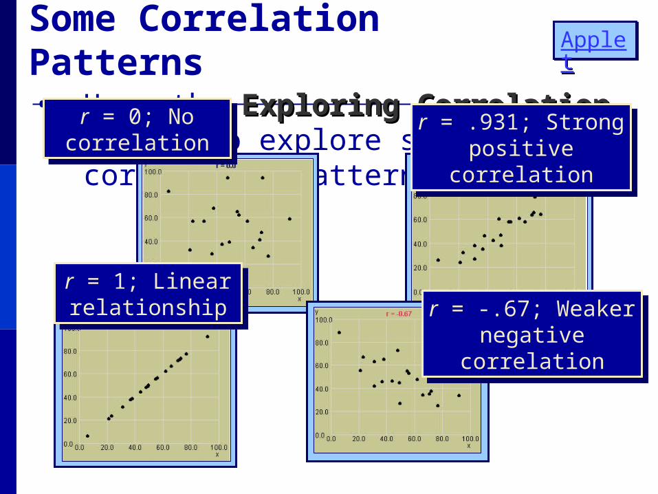
Some Correlation Patterns • Use the Exploring CorrelationExploring Correlation applet to
explore some correlation patterns:
AppletApplet
r = 0; No correlation
r = 0; No correlation
r = .931; Strong positive correlation
r = .931; Strong positive correlation
r = 1; Linear relationship
r = 1; Linear relationship r = -.67; Weaker
negative correlation
r = -.67; Weaker negative correlation
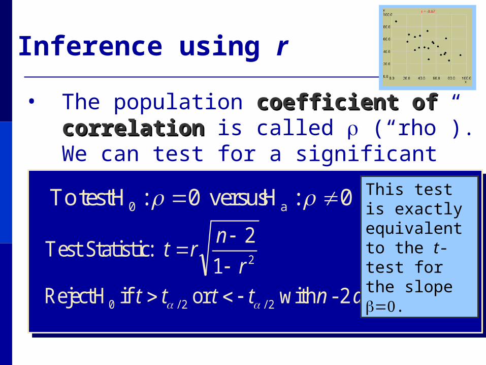
Inference using r
• The population coefficient of correlationcoefficient of correlation is called (“rho”). We can test for a significant correlation between x and y using a t test:
0:H versusH test To a0 0:
. 2- withor if H Reject
:Statistic Test
0 dfnttttr
nrt
2/2/
21
2
This test is exactly equivalent to the t-test for the slope .
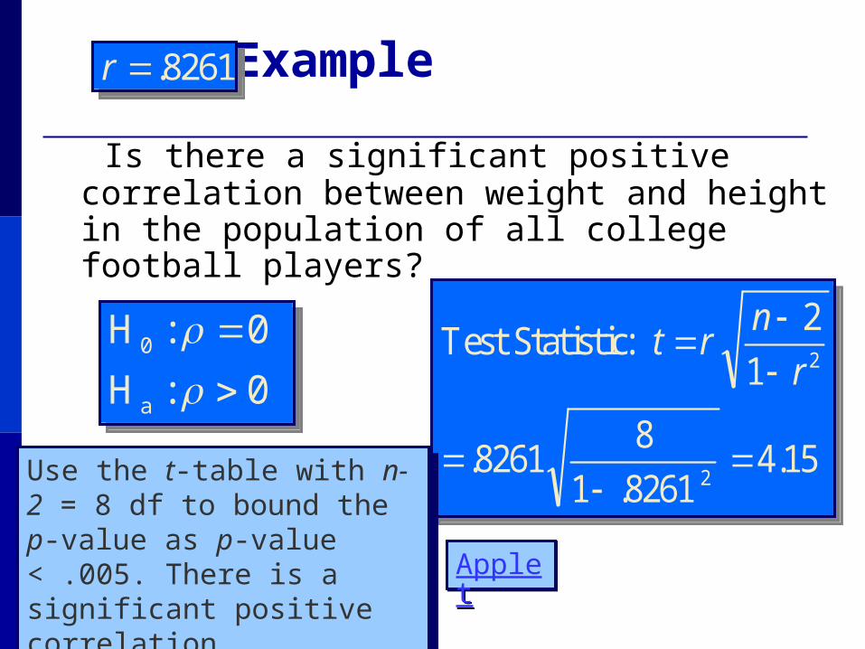
Example
Is there a significant positive correlation between weight and height in the population of all college football players?
8261.r 8261.r
0:H
H
a
0
0:
0:H
H
a
0
0:
15.48261.1
88261.
1
2
2
2
:Statistic Testr
nrt
15.48261.1
88261.
1
2
2
2
:Statistic Testr
nrt
Use the t-table with n-2 = 8 df to bound the p-value as p-value < .005. There is a significant positive correlation.
Use the t-table with n-2 = 8 df to bound the p-value as p-value < .005. There is a significant positive correlation. AppletApplet