1

Introduction to Probability – 2018/19

These notes are a summary of what is lectured. They do not contain all examples or

explanations and are NOT a substitute for your own notes. The notes are largely based

on previous versions of the module by courtesy of Robert Johnson.

2

§0 Introduction

Before starting the module properly we will spend a bit of time thinking about what

probability is and where it is used.

Example 0.1 How many people do you need in a room to have a better than 50% chance

that two of them share a birthday?

This is a simple calculation which we will see how to do later. If you haven’t seen this

before then try to guess what the answer will be. Most people have rather poor intuition

for this kind of question so I would expect there to be a wide range of guesses and for

many of them to be far from the true answer.

Example 0.2 Would you rather be given £5, or toss a coin winning £10 if it comes up

heads?

Would you rather be given £5000, or toss a coin winning £10000 if it comes up heads?

Would you rather be given £1, or toss a coin 10 times winning £1000 if it comes up heads

every time?

This example is not entirely a mathematical one and there is no right or wrong answer

for each part. However some tools from probability can help to describe the choice we

have quantitatively. In each case the average amount we expect to win and the degree of

variation in our gain are relevant. Properties of so called random variables can be used

to describe this choice. Of course there are lots of extra ingredients which will influence

our choice (for instance how useful a particular sum of money is to us, and how much

we enjoy the excitement of taking a risk). One attempt to model some of these extra

factors mathematically is the idea of utility functions from game theory (this is beyond

the module).

Example 0.3 A suspect’s fingerprints match those found on a murder weapon. The

chance of a match occurring by chance is around 1 in 50,000. Is the suspect likely to be

innocent?

3

The third example emphasises how important it is to work out exactly what information

we are given and what we want to know. The court would have to consider the probability

that the suspect is innocent under the assumption that the fingerprints match. The

numerical probability given in the question is the probability that the fingerprints match

under the assumption that the suspect is innocent. These are in general completely

different quantities. The erroneous assumption that they equal is sometimes called the

prosecutor’s fallacy. The mathematical tool for considering probabilities given certain

assumptions is conditional probability.

These questions all relate to situations where there is some randomness; that is events

we cannot predict with certainty. This could be either because they happen by chance

(tossing a coin) or they are beyond our knowledge (the innocence or guilt of a suspect).

Probability theory is about quantifying randomness.

The question of what probability is does not have an entirely satisfactory answer. We

will associate a number to an event which will measure the likelihood of it occurring. But

what does this really mean? You can think of it some kind of limiting frequency.

Informal definition of a probability: repeat an experiment (say roll a die) N times. Let

A denote an event (say the die shows an even number). Suppose the event comes up m

times (among the N repetitions of the experiment). Then the ratio m/N (in the limit of

very large values N) denotes the probability of the event A.

We will later give a precise mathematical definition of which roughly speaking defines

probability in terms of the properties it should have.

§1 Sample Space and Events

The general setting is we perform an experiment and record an outcome. Outcomes must

be precisely specified, mutually exclusive and cover all possibilities.

Definition 1.1 The sample space is the set of all possible outcomes for the experiment.

It is denoted by S (or S or Ω).

Definition 1.2 An event is a subset of the sample space. The event occurs if the actual

4

outcome is an element of the set.

Example 1.1 Roll a die (experiment) and write down the number showing (outcome).

The sample space is the set containing 1,2,3,4,5,6

S = 1, 2, 3, 4, 5, 6 .

The event A = 2, 4, 6 corresponds to the rolling of an even number.

Example 1.2 A coin is tossed three times and the sequence of heads/tails is recorded.

S = hhh, hht, hth, htt, thh, tht, tth, ttt

where, for example, htt means the first toss is a head, the second is a tail, the third is a

tail.

If A is the event “exactly one head seen” then

A = htt, tht, tth.

Equivalently we could take

S ′ = 1, 2, 3, 1, 2, 1, 3, 2, 3, 1, 2, 3,

where we record the set of tosses which are head. The outcome 1, 3 means hth.

B = 1, 2, 2, 2, 3, 1, 2, 3

is the event “the second toss is a head”.

Example 1.3 Take an exam repeatedly until you pass.

S = P, FP, FFP, FFFP, . . .

where we record the sequence of fails and passes. S is infinite.

Other ways representing the sample space: record the number of attempts

S ′ = 1, 2, 3, 4, . . .

Record the number of fails

S ′′ = 0, 1, 2, 3, . . .

5

Among other things these examples illustrate that the sample space may be finite or

infinite, and that sometimes there were several equally good ways to describe outcomes.

Definition 1.3 An event E is a simple event (or elementary event) if it consists of a

single element of the sample space S.

Example 1.4 In example 1.3 the event “pass first time”, E = P, is a simple event.

Basic set theory: We use extensively the terminology and notation of basic set theory.

Informally a set is an unordered collection of well- defined distinct objects. For instance

b,−2.4, is a set. Strictly speaking 2, 3, 3 is not a set (sometimes people use slang

and mean by these symbols the two element set 2, 3). 2, 3, 5, 1 and 3, 5, 2, 1 are the

same sets as order does not matter. Two sets, A and B are equal, A = B,if they contain

precisely the same elements. A set can be specified in various ways.

• By listing the objects in it between braces (, ) separated by commas, e.g., 1, 2, 3, 4.

• (usually for infinite sets) By listing enough elements to determine a pattern, e.g.,

2, 4, 6, 8, . . . (the set of positive even integers). A set which can be written as a

comma separated list is said to be countable.

• By giving a rule, e.g., x : x is an even integer (read as “the set of all x such that

x is an even integer”).

If A is a set we write x ∈ A to mean that the object x is in the set A and say that x is

an element of A. If x is not an element of A then we write x 6∈ A.

Let A and B be sets.

• A ∪B (“A union B”) is the set of elements of A or B (or both)

A ∪B = x : x ∈ A or x ∈ B

• A ∩B (“A intersection B”) is the set of elements of both A and B

A ∩B = x : x ∈ A and x ∈ B

6

• A \B (“A take away B”) is the set of elements in A but not in B

A \B = x : x ∈ A and x 6∈ B

• A4B (“symmetric difference of A and B”) is the set of elements in either A or B

but not both

A4B = (A \B) ∪ (B \ A)

• If all the elements of A are contained in the set B we say that A is a subset of B,

A ⊆ B.

• If all sets are subsets of some fixed set S then Ac (“the complement of A”) is the

set of all elements of S which are not elements of A.

Ac = S \ A

• If A = a1, a2, . . . , an denotes a finite set of n elements then |A| = n denotes the

size (or cardinality) of the set (do not confuse the size of a set with the absolute

value of a number).

• We say two sets A and B are disjoint if they have no element in common, i.e.,

A ∩B = ∅

where ∅ = denotes the empty set.

Events: Let A and B denote events (i.e. subsets of the sample space S).

• If A is an event then Ac contains the elements of the sample space which are not

contained in A, i.e., Ac is the event that “A does not occur”.

• If A and B are events then the event E “A and B both occur” consists of all elements

of both A and B, i.e., E = A ∩B.

• The event E “at least one of A or B occurs” consists of all elements in A or B, i.e.,

E = A ∪B.

• The event E “A occurs but B does not” consists of all elements in A but not in B,

i.e., E = A \B.

7

• The event E “exactly one of A or B occurs” consists of all elements in A or B but

not in both, i.e., E = A4B.

Example 1.5 Roll a die, let A be the event that an even number occurs (see example

1.1) and B the event that the outcome is a prime number

B = 2, 3, 5

Denote by E1 the event that “the outcome is an even number or a prime” then

E1 = A ∪B = 2, 3, 4, 5, 6

Denote by E2 the event that “the outcome is either an even number or a prime” then

E2 = A4B = 3, 4, 5, 6

8

§2 Properties of Probabilities

We want to assign a numerical value to an event which reflects the chance that it occurs.

Probability is a concept/recipe (or in formal terms a function) P which assigns a (real)

number P(A) to each event A, 0 ≤ P(A) ≤ 1.

The simplest way of doing this is to say that the probability of an event A is the ratio

of the number of outcomes in A to the total number of outcomes in S. We sometimes

describe this as the situation where all outcomes are equally likely.

Example 2.1 Roll a die, sample space S = 1, 2, 3, 4, 5, 6. Consider the event A “the

number shown is smaller than 3”, A = 1, 2. Define the probability of A by

P(A) =|A||S|

=2

6=

1

3

Sometimes this is a reasonable thing to do but often it is not. In the example 2.1 above

if the die is biased however this would not be a reasonable notion of probability.

We also run into difficulties if S is infinite. If S = N (the set of positive integers), see

example 1.3 then there is no reasonable way to choose an element of S with all outcomes

equally likely. There are however ways to choose a random positive integer in which every

outcome has some chance of occurring.

The formal approach is to regard probability as a mathematical construction satisfying

certain axioms.

Definition 2.1 (Kolmogorov’s Axioms for Probability) Probability is a function P

which assigns to each event A a real number P(A) such that:

a) For every event A we have P(A) ≥ 0,

b) P(S) = 1,

c) If A1, A2, . . . , An are n pairwise disjoint events (Ak ∩ A` = ∅ for all k 6= `) then

P(A1 ∪ A2 ∪ · · · ∪ An) = P(A1) + P(A2) + . . .+ P(An) =n∑k=1

P(Ak).

9

Remark:

• The function P is sometimes called a probability measure.

• We say that events satisfying definition 2.1c are pairwise disjoint or mutually exclu-

sive.

• Notice that definition 2.1c has a version for a countable infinite number of events as

well, which we do not cover in this module (e.g. we would need to clarify the notion

of an infinite sum first). Further subtleties occur if S is infinite (more particularly

if it is not countable).

Example 2.2 Suppose that the sample space S is finite. Then the setting

P(A) =|A||S|

gives a probability. This is the case when every outcome in the sample space is equally

likely (we say we pick an outcome at random). We need to show that this setting obeys

definition 2.1.

a) If A ⊆ S then |A| ≥ 0 and

P(A) =|A||S|≥ 0

|S|= 0

b)

P(S) =|S||S|

= 1

c) If A1, A2, . . . An are pairwise disjoint subsets of S then

|A1 ∪ A2 ∪ . . . ∪ An| = |A1|+ |A2|+ . . .+ |An|

and

P(A1 ∪ A2 ∪ . . . ∪ An) =|A1|+ |A2|+ . . .+ |An|

|S|

=|A1||S|

+|A2||S|

+ . . .+|An||S|

= P(A1) + P(A2) + . . .P(An)

10

In this situation calculating probabilities becomes counting!

Warning: In general, do not assume that outcomes are equally likely without good

reason.

Example 2.3 Toss a biased coin. The sample space is given by S = h, t. P(∅) = 0,

P(h) = 1/3, P(t) = 2/3, and P(S) = 1 defines a probability measure.

Starting from the axioms we can deduce various properties. Hopefully, these will agree

with our intuition about probability (if they did not then this would suggest that we had

not made a good choice of axioms). The proofs of all of these are simple deductions from

the axioms.

Proposition 2.1 If A is an event then

P(Ac) = 1− P(A).

The statement makes perfect sense. If P(A) is the probability of the event A then the

probability of the complementary event Ac should be 1−P(A). If we are able to provide a

formal proof then we have evidence that definition 2.1 is consistent with real world setups.

Proof: Let A be any event. Set A1 = A and A2 = Ac. By definition of the complement

A1 ∩ A2 = ∅ and so we can apply definition 2.1c (with n = 2) to get

P(A1 ∪ A2) = P(A1) + P(A2) = P(A) + P(Ac).

But (again by definition of the complement) A1 ∪ A2 = S so by definition 2.1b

1 = P(S) = P(A1 ∪ A2).

Combining both expressions

1 = P(A) + P(Ac).

Rearranging this gives the result. .

We can use the results we have proved to deduce further ones such as the following ones.

These are called corollaries as they are an “obvious” consequence of the proposition 2.1.

11

Corollary 2.1

P(∅) = 0.

This statement makes perfect sense as well. The probability of “nothing” is zero.

Proof: By definition of complement Sc = S \ S = ∅. Hence by Proposition 2.1

P(∅) = P(Sc) = 1− P(S)

Using definition 2.1b we have

P(∅) = 1− 1 = 0

.

Corollary 2.2 If A is an event then P(A) ≤ 1.

Again the statement sounds sensible. Probabilities are always smaller or equal to one.

Proof: By proposition 2.1

P(Ac) = 1− P(A).

But Ac is an event, so by definition 2.1a

0 ≤ P(Ac) = 1− P(A)

and hence

P(A) ≤ 1

.

The following statements are less obvious consequences of definition 2.1 and the statements

we have shown so far. Thus we call them again propositions.

Proposition 2.2 If A and B are events and A ⊆ B then

P(A) ≤ P(B).

12

This statement looks sensible as well. If an event B contains all the outcomes of an event

A then the former has the higher probability.

Proof: Consider the events A1 = A and A2 = B \A. Then A1 ∩A2 = ∅ (the two events

are pairwise disjoint) and A1 ∪ A2 = B. So by definition 2.1c (with n = 2)

P(B) = P(A1 ∪ A2) = P(A1) + P(A2) = P(A) + P(B \ A)

Since B \ A is an event definition 2.1a tells us that

P(B)− P(A) = P(B \ A) ≥ 0

The statement follows by rearrangement. .

Proposition 2.3 If A = a1, a2, . . . , an is a finite event then

P(A) = P(a1) + P(a2) + . . .+ P(an) =n∑i=1

P(ai).

The statement is quite remarkable. The probability of a (finite) event is the sum of the

probabilities of the corresponding simple events. One often writes P(ai) for P(ai) even

though the former one is incorrect.

Proof: Denote by Ai = ai, i = 1, .., n the simple events. The events are pairwise

disjoint and A1 ∪ A2 ∪ . . . ∪ An = A. So by definition 2.1c

P(A) = P(A1∪A2∪. . .∪An) = P(A1)+P(A2)+. . .+P(An) = P(a1)+P(a2)+. . .+P(an)

.

Proposition 2.4 (Inclusion-exclusion for two events) For any two events A and B

we have

P(A ∪B) = P(A) + P(B)− P(A ∩B).

The statement is not entirely obvious. For general events the probability of the event “A

or B” is normally not the sum of the probabilities of events A and B. Because of some

“double counting” one needs to correct by the probability of the event “A and B”.

13

Proof: Consider the three events E1 = A \B, E2 = A∩B and E3 = B \A. The events

are pairwise disjoint and E1 ∪ E2 ∪ E3 = A ∪B. Hence by definition 2.1c (with n = 3)

P(A ∪B) = P(E1) + P(E2) + P(E3) .

Furthermore E1 ∪ E2 = A and E2 ∪ E3 = B. Thus definition 2.1c (with n = 2) yields

P(A) = P(E1) + P(E2)

P(B) = P(E2) + P(E3) .

Since P (A ∩B) = P(E2) we finally have

P(A) + P(B)− P(A ∩B) = P(E1) + P(E2) + P(E2) + P(E3)− P(E2)

= P(E1) + P(E2) + P(E3) = P(A ∪B) .

.

Example 2.4 Consider a finite sample space S with probability

P(E) =|E||S|

.

Example 2.2 tells us that in this case definition 2.1 is fulfilled and in particular proposition

2.4 applies. Let A ⊆ S and B ⊆ S denote two events then proposition 2.4 reads

|A ∪B||S|

=|A||S|

+|B||S|− |A ∩B|

|S|

that means

|A ∪B| = |A|+ |B| − |A ∩B| .

This last statement is a statement about the sizes of finite sets (which can be proven in

other ways as well). Hence probability theory can give results which do not involve any

“randomness”. This cross fertilisation is essentially what mathematics is about.

Proposition 2.5 (Inclusion-exclusion for three events) For any three events A,B

and C we have

P(A∪B ∪C) = P(A) +P(B) +P(C)−P(A∩B)−P(A∩C)−P(B ∩C) +P(A∩B ∩C).

14

As for two events there exists an “intuitive” argument but that is not a proof.

Proof: Essentially we will apply proposition 2.4 three times. Let D = A ∪ B so that

A ∪B ∪ C = C ∪D. Then

P(A ∪B ∪ C) = P(C ∪D)

= P(C) + P(D)− P(C ∩D) by proposition 2.4

= P(C) + P(A ∪B)− P(C ∩D)

= P(C) + P(A) + P(B)− P(A ∩B)− P(C ∩D) by proposition 2.4

Now C ∩D = C ∩ (A ∪B) = (C ∩ A) ∪ (C ∩B) so that

P(C ∩D) = P((C ∩ A) ∪ (C ∩B))

= P(C ∩ A) + P(C ∩B)− P((C ∩ A) ∩ (C ∩B)) by proposition 2.4

= P(C ∩ A) + P(C ∩B)− P(A ∩B ∩ C)

Combining both expressions

P(A∪B ∪C) = P(C) + P(A) + P(B)− P(A∩B)− P(C ∩A)− P(C ∩B) + P(A∩B ∩C)

.

Remark: There is also an inclusion-exclusion formula for n events. If you like work out

this formula and try to prove it (but it won’t be easy).

Example 2.5 Suppose that the probabilities for each of the three events A, B, and C is

1/3, i.e.

P(A) = P(B) = P(C) =1

3.

Furthermore assume that the probabilities for each of the events “A and B”, “A and C”,

and “B and C” is 1/15, i.e.,

P(A ∩B) = P(A ∩ C) = P(B ∩ C) =1

15.

What can be said about the probability of the event that none of A, B, or C occur?

15

The event we are interested in is the event (A ∪B ∪ C)c. Hence

P((A ∪B ∪ C)c) = 1− P(A ∪B ∪ C) by proposition 2.1

= 1− [P(A) + P(B) + P(C)− P(A ∩B)−

P(A ∩ C)− P(B ∩ C) + P (A ∩B ∩ C)] by proposition 2.5

= 1−[

1

3+

1

3+

1

3− 1

15− 1

15− 1

15+ P (A ∩B ∩ C)

]=

1

5− P (A ∩B ∩ C) .

Since A ∩B ∩ C ⊆ A ∩B, definition 2.1a and proposition 2.2 tell us that

0 ≤ P (A ∩B ∩ C) ≤ P(A ∩B) =1

5.

So2

10≤ P((A ∪B ∪ C)c) ≤ 3

10.

Note that the bounds are sharp, i.e., there are examples where equality is possible. Con-

sider for instance the sample space S = 1, 2, 3, 4, 5, 6, 7, 8, 9, 10, 11, 12, 13, 14, 15 with

all outcomes being equally likely. Events A = 1, 2, 3, 4, 5, B = 5, 6, 7, 8, 9, C =

1, 9, 10, 11, 12 satisfy the conditions of the example and P((A ∪B ∪ C)c) = 1/5.

Remark: The various properties of probabilities derived in this paragraph are just based

on the basic definition 2.1. Hence few simple axioms can lead to a plethora of results (such

structures is essentially what mathematics is about).

16

§3 Sampling

When all elements of the sample space are equally likely calculating probability often

boils down to counting the number of ways of making some selection, see example 2.2.

Specifically, we are often interested in finding how many ways there are of choosing r

things from an n element set. This is called sampling from an n element set. The answer

to this question depends on exactly what we mean by selection: is the order important

and is repetition allowed.

a) Ordered Sampling with Replacement

Example 3.1 How many flags are there consisting of 3 vertical stripes each of which is

red, blue, green or white (and if we allow adjacent stripes to be of the same colour)?

This is an ordered selection of 3 things from a set of 4 things with repetition allowed.

There are 4 choices for the first stripe. For each of these there are 4 choices of the second

stripe, and for each of these there are 4 choices for the 3rd stripe. In total there are

4× 4× 4 = 43 = 64 flags.

• A set is an unordered collection of different objects. Consider a set U = u1, u2, . . . , un

of n elements, |U | = n.

• An ordered selection from the set U of r objects which are not necessarily distinct,

(u1, u2, . . . , ur) is called an r-tuple. For instance (3,−1, 3, 5) and (3, 3,−1, 5) are

different 4-tuples. A 2-tuple (u1, u2) is called a pair (e.g. coordinates in the Cartesian

plane).

• If we make an ordered selection of r things from a set U with replacement allowed

(that is to say we allow elements to be repeated) then the sample space is the set

of all ordered r-tuples of elements of U . That is

S = (u1, u2, . . . , ur) : ui ∈ U,

• If |U | = n there are n choices for u1, for each of these there are n choices for u2,

and so on. Hence, we have

|S| = |U |r = nr.

17

b) Ordered Sampling without Replacement

Example 3.2 Suppose that in example 3.1 we are not allowed to repeat a colour. There

are 4 choices for the first stripe. For each of these there are 3 choices for the second stripe,

and for each of these there are 2 choices for the 3rd stripe. In total there are 4×3×2 = 24

flags.

• Consider a set U = u1, u2, . . . , un of size |U | = n.

• If we make an ordered selection of r things from a set U without replacement (that

is to say we do not allow elements to be repeated) then the sample space is the set

of all ordered r-tuples of distinct elements of U . That is

S = (u1, u2, . . . , ur) : ui ∈ U with ui 6= uj for all i 6= j.

• To find the cardinality of this notice that if |U | = n there are n choices for u1, for

each of these choices there are n− 1 choices for u2, for each of these there are n− 2

choices for u3 and so on. Hence,

|S| = n× (n− 1)× (n− 2)× · · · × (n− r + 1)

=n× (n− 1)× (n− 2×) . . .× (n− r + 1)× (n− r)× (n− r − 1)× . . .× 2× 1

(n− r)× (n− r − 1)× . . .× 2× 1

=n!

(n− r)!

where k! = k × (k − 1)× . . .× 2× 1 (“k factorial”) with the convention 0! = 1.

Example 3.3 How many permutations of (1, 2, . . . , n) are there? A permutation is an

ordered sample of n things from the set U = 1, 2, . . . , n of n things, i.e., we sample

r = n objects without replacement. So there are n × (n − 1) × . . . × 2 × 1 = n!/0! = n!

permutations.

c) Unordered Sampling without Replacement

Example 3.4 How many ways are there to choose 5 players for a penalty shootout from

a team of 11 football players (goalkeeper is permitted).?

18

If we were to pick the players in shooting order we would make an ordered selection without

replacement. So there are 11!/6! ways to do this. Given there are 5 players there are 5!

ways to arrange it into shooting order. So 5! × number of possibilities = 11!/6! and the

number of possibilities is 11!/(6!× 5!).

• Consider a set U = u1, u2, . . . , un of size |U | = n.

• If we make an unordered selection of r things from a set U without replacement

then we obtain a subset A = u1, u2, . . . , ur of U of size r.

• The corresponding sample space is the set of all subsets of r distinct elements of U .

S = A ⊆ U : |A| = r.

• An ordered sample is obtained by taking an element of this sample space S and

putting its elements in order. Each element of the sample space can be ordered in

r! ways and so (using the formula for ordered selections with repetition, see section

3b, and assuming |U | = n) we have that

r!× |S| = n!

(n− r)!,

and so

|S| = n!

(n− r)!r!.

Remark: This expression is usually written as(n

r

)=

n!

(n− r)!r!

(read as “n choose r”) and is called a binomial coefficient. By convention(nr

)= 0 when

r > n. Binomial coefficients appear for instance in the binomial theorem

(a+ b)n =

(n

0

)anb0 +

(n

1

)an−1b1 +

(n

2

)an−2b2 + . . .+

(n

n− 1

)a1bn−1 +

(n

n

)a0bn

=n∑k=0

(n

k

)akbn−k .

Try to verify this formula for n = 2 or n = 3, and if you like prove the expression (e.g.

by induction).

19

d) Summary

To summarise we have shown the following

Theorem 3.1 The number of ways of selecting (sampling) r things from an n element

set is

a) ordered with replacement/repetition allowed: nr

b) ordered without replacement/no repetition : n!/(n− r)!

c) unordered without replacement/no repetition :(nr

)

Remark: We have not covered/proven the case of unordered sampling with replace-

ment/repetition. This case is rather elaborate to deal with.

Example 3.5 You have 10 coins, 7 silver ones and 3 copper ones, and you pick 4 coins

at random (i.e. all outcomes are equally likely). Let

• D be the event that you pick 4 silver coins,

• E be the event that you pick 2 silver coins followed by 2 copper coins,

• F be the event that you pick 2 silver and 2 cooper coins in any order.

Find P(D), P(E), and P(F ).

Since we pick coins at random P(A) = |A|/|S|. So wee need to determine the size of the

sample space and the size of the event.

The set U of objects contains 7 (in principle distinct) silver coins and 3 (distinct) copper

coins, U = c1, c2, c3, s1, s2, . . . , s6, s7. It is important to note that we are going to sample

from such a set (and by definition elements of sets are distinct, even though 7 elements

have the same property, namely being silver, and 3 have the same property, namely being

copper).

20

i) Let us consider the experiment as ordered sampling (that is definitely required for

event E, for the others we have choices) without replacement. Outcomes are an

ordered selection of 4 objects, i.e., a 4-tuple (u1, u2, u3, u4) with uk ∈ U . Since

n = 10 and r = 4 (in each case we pick 4 coins) the size of the sample space is,

according to theorem 3.1b

|S| = 10!

6!= 10× 9× 8× 7 .

Consider event D. The outcome in D is an ordered sample of 4 things from the

(sub)set of 7 silver coins (without replacement), for instance (s5, s2, s6, s3). Accord-

ing to theorem 3.1b

|D| = 7!

3!= 7× 6× 5× 4

so

P(D) =|D||S|

=7× 6× 5× 4

10× 9× 8× 7=

1

6.

Consider event E. An outcome in E is of the form (si, sj, ck, c`).

– There are 7 choices for si.

– For each of these there are 6 choices for sj.

– For each of these there are 3 choices for ck.

– For each of these there are 2 choices for c`.

So

|E| = 7× 6× 3× 2

and

P(E) =|E||S|

=7× 6× 3× 2

10× 9× 8× 7=

1

20.

Consider event F . There are 6 possible patterns to select 2 silver and 2 copper coins,

namely sscc, scsc, sccs, cssc, cscs, and ccss and each occurs in 7× 6× 3× 2 ways

(see the previous event). So

|F | = 6× 7× 6× 3× 2

and

P(F ) =|F ||S|

=6× 7× 6× 3× 2

10× 9× 8× 7=

3

10.

21

ii) Let us consider the experiment as unordered sampling without replacement. That is

simpler, but we cannot cover event E as there the order is important. Outcomes are

now 4-element subsets u1, u2, u3, u4 with uk ∈ U . Since n = 10 and r = 4 the size

of the sample space is, according to theorem 3.1c

|S| =(

10

4

)=

10× 9× 8× 7

4× 3× 2× 1.

Consider event D. Outcomes in D are cm, cn, ck, c`, i.e., 4 element subsets taken

from the set of 7 copper coins. We sample r = 4 coins from a (sub)set of n = 7

coins. So

|D| =(

7

4

)=

7× 6× 5× 4

4× 3× 2× 1

and

P(D) =|D||S|

=

(74

)(104

) =7× 6× 5× 4

10× 9× 8× 7=

1

6

(of course the same result as in i)).

Consider event F . An outcome in F has the form sm, sn, ck, c` = sm, sn ∪

ck, c`. According to theorem 3.1c there are(72

)ways to select 2 silver coins from

a (sub)set of 7, and(32

)ways to select 2 copper coins from a (sub)set of 3. Thus

|F | =(

7

2

)(3

2

)=

7× 6× 3× 2

2× 1× 2× 1

and

P(F ) =|F ||S|

=

(72

)(32

)(104

) =7× 6× 3× 2× 4× 3× 2

10× 9× 8× 7× 2× 2=

3

10

(of course again the same result).

Example 3.6 (The birthday problem) Ask 30 people for their birthday (assume no-

body is born on 29 February). Let A be the event that there is a repeated birthday, and Ac

be the event that there is no repeated birthday.

Let us consider the experiment as ordered sampling from a set of n = 365 days. An

outcome in the sample space is a 30-tuple (u1, u2, . . . , u30) with uk denoting the respective

birthday. The size of the sample space is, according to theorem 3.1a

|S| = 36530 .

22

Consider the event Ac, i.e. a ordered selection of birthdays (u1, u2, . . . , u30) without repe-

tition. The outcomes of the event Ac are ordered samples of size r = 30 without replace-

ment/repetition (as Ac contains non repeated birthdays only) from a set of size n = 365.

According to theorem 3.1a

|Ac| = 365!

335!= 365× 364× 363× . . .× 337× 336 .

Thus

P(A) = 1− P(Ac) by proposition 2.1

= 1− |Ac||S|

= 1− 365

365× 364

365× 363

365× . . .× 337

365× 336

365

= 0.70631624 . . .

and the probability of a repeated birthday among 30 people is more than 70%.

Example 3.7 (Poker dice) You roll 5 dice. Find the probability to roll “a pair” (that

means outcomes of the type e.g. 33152 etc.).

We are sampling r = 5 objects from the set U = 1, 2, 3, 4, 5, 6 of size n = 6. We sample

with replacement/repetition, so consider ordered sampling with replacement.

Size of the sample space, theorem 3.1a

|S| = |U |r = 65 .

Denote by A the event to “roll a pair”. Consider first those outcomes in the event A which

have the pair as the first two entries, i.e., outcomes (p, p, r1, r2, r3). There are 6 choices

for p, for each of those there are 5 choices for r1, for each of those there are 4 choices

for r2, for each of those there are 3 choices for r3. Hence there are 6× 5× 4× 3 of such

outcomes.

But A contains as well outcomes where the pair does not come as the first two entries, i.e.,

outcomes which differ from the pattern pprrr. There are in total “5 choose 2” different

patterns pprrr, prprr, prprr,. . . , rrrpp, each giving rise to 6×5×4×3 outcomes. Hence

|A| = 10× 6× 5× 4× 3 .

23

Thus

P(A) =|A||S|

=10× 6× 5× 4× 3

65=

25

54.

Remark: It is important when answering questions involving sampling that you read

the question carefully and decide what sort of sampling is involved. Specifically, how

many things are you selecting, what set are you selecting from, does the order matter,

and is repetition allowed or not. Sometimes more than one sort can be used but you must

be consistent (see the previous example 3.5).

24

§4 Conditional Probability

Additional information (a so called “condition”) may change the probability of an event.

Example 4.1 Roll a fair die. Sample space

S = 1, 2, 3, 4, 5, 6

Consider event A “the number shown is odd”

A = 1, 3, 5, P(A) =|A||S|

=1

2

and event B “the number shown is smaller than 4”

B = 1, 2, 3, P(B) =|B||S|

=1

2

Suppose we roll the die and somebody tells us that the number shown is odd (i.e. event A

has happened/ event A is given). Now the probability of event B (given event A) is

P(B given event A) =|1, 3||1, 3, 5|

=2

3

How is this expression linked with P(A), P(B), . . . ?

P(B given event A) =|1, 3||1, 3, 5|

=|1, 3|/|S||1, 3, 5|/|S|

=|1, 3|/|S|

P(A)=|A ∩B|/|S|

P(A)=

P(A ∩B)

P(A)

The expression P(B given event A) = P(B|A) is called conditional probability.

Example 4.2 You have three pens coloured blue, red, and green. You pick one at random,

then you pick another without replacement. Size of the sample space

|S| = 3× 2 = 6

Let A be the event that the first pen is red. Let B be the event that the second pen is blue.

P(A) =|rb, rg||S|

=1

3

P(B) =|rb, gb||S|

=1

3

P(A ∩B) =|rb||S|

=1

6

25

Clearly P(A ∩B) 6= P(A)P(B)

Now assume we know that event A has happened (i.e. the first pick was a red pen). The

probability for the event B (with the condition that A has happened) is 1/2 (picking at

random a blue pen from the remaining two pens) and P(A ∩B) = P(A)× 1/2 ! Here

1

2=|rb||rb, rg|

=|A ∩B||A|

=P(A ∩B)

P(A)

and such a quantity is called a conditional probability (the probability for the event B

conditioned on A has occurred).

Definition 4.1 If A and B are events and P(A) 6= 0 then the conditional probability of

B given A, usually denoted by P(B|A), is

P(B|A) =P(A ∩B)

P(A).

Remark:

• The notation P(A|B) is very unfortunate. A|B is not an event, it has no meaning !

Do not confuse the conditional probability P(A|B) with P(A \ B), the probability

for the event “A and not B”.

• Note that the definition does not require that B happens after A. In example 4.2 it

would make sense to talk about P(A|B) = P(A∩B)/P(B), the probability that the

first pen is red given that the second pen is blue. One way of thinking of this is to

imagine that the experiment is performed secretly and the fact that A occurred is re-

vealed to you (without the full outcome being revealed). The conditional probability

of B given A is the new probability of B in these circumstances.

• Conditional probability can be used to measure how the occurrence of some event

influences the chance of another event occurring.

If P(B|A) < P(B) then A occurring makes B less probable.

If P(B|A) > P(B) then A occurring makes B more probable.

If P(B|A) = P(B) then the event A has no impact on the probability of event B

(see section 5).

26

• In some cases we will use the conditional probability P (B|A) to calculate P(A∩B),

in some cases we will use P(A ∩B) to find the conditional probability P(B|A).

Example 4.3 Roll a fair die (“pick at random”) twice. Consider the events

• A: “first roll is a 6”

• B: “roll a double”

• C: “roll at least one odd number”

So (if considered as ordered sampling)

|S| = 36

and

P(A) =1

6, P(B) =

1

6, P(C) =

3

4

P(A ∩B) =1

36, P(B ∩ C) =

1

12, P(A ∩ C) =

1

12

Conditional probability of a double given that first roll is a 6

P(B|A) =P(B ∩ A)

P(A)=

1/36

1/6=

1

6.

This is somehow obvious.

Conditional probability to roll a 6 first given that one rolls a double

P(A|B) =P(A ∩B)

P(B)=

1

6.

Slightly less obvious. Note that conditional probability does not require the condition to

happen “first” (here event B happens “after” event A has happened). Conditional proba-

bility does not assume any causality.

Conditional probability to roll at least one odd given that one rolls a double

P(C|B) =P(C ∩B)

P(B)=

1

2.

27

Somehow obvious.

Conditional probability to roll a double given that one rolls at least one odd

P(B|C) =P(B ∩ C)

P(C)=

1

9.

Probably not obvious at all.

Notice P(C|B) < P(C) so the information that a double is rolled makes it less likely to

see an odd number. And P(B|C) < P(B), so the information that an odd number is seen

makes it less likely to have rolled a double.

But P(B|A) = P(B) and P(A|B) = P(A). That means rolling a 6 first does not change

the chance of seeing a double, and rolling a double does to change the chance of having

rolled a 6 first. Events with such a property will be called independent and we will discuss

the issue in detail in the next section.

Example 4.4 Reconsider the event D in example 3.5 (picking 4 silver coins from a set

of 7 silver and 3 copper coins). We can work out P(D) using conditional probability.

Let Ai be the event that the ith coin picked is a silver coin. Obviously D = A1∩A2∩A3∩A4.

P(A1) =7

10.

If A1 occurs then the 2nd pick is a coin from 9 of which 6 are silver. So

P(A2|A1) =6

9

and by the definition 4.1 of the conditional probability we have

P(A1 ∩ A2) = P(A1)P(A2|A1) =7

10× 6

9.

If A1 and A2 occur then the third pick is from 8 coins 5 of which are silver so

P(A3|A1 ∩ A2) =5

8.

Again the definition of conditional probability tells us that

P(A1 ∩ A2 ∩ A3) = P(A1 ∩ A2)P(A3|A1 ∩ A2) =7

10× 6

9× 5

8.

28

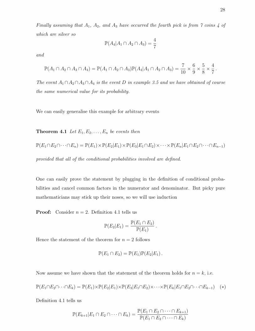
Finally assuming that A1, A2, and A3 have occurred the fourth pick is from 7 coins 4 of

which are silver so

P(A4|A1 ∩ A2 ∩ A3) =4

7

and

P(A1 ∩ A2 ∩ A3 ∩ A4) = P(A1 ∩ A2 ∩ A3)P(A4|A1 ∩ A2 ∩ A3) =7

10× 6

9× 5

8× 4

7.

The event A1∩A2∩A3∩A4 is the event D in example 3.5 and we have obtained of course

the same numerical value for its probability.

We can easily generalise this example for arbitrary events

Theorem 4.1 Let E1, E2, . . . , En be events then

P(E1∩E2∩· · ·∩En) = P(E1)×P(E2|E1)×P(E3|E1∩E2)×· · ·×P(En|E1∩E2∩· · ·∩En−1)

provided that all of the conditional probabilities involved are defined.

One can easily prove the statement by plugging in the definition of conditional proba-

bilities and cancel common factors in the numerator and denominator. But picky pure

mathematicians may stick up their noses, so we will use induction

Proof: Consider n = 2. Definition 4.1 tells us

P(E2|E1) =P(E1 ∩ E2)

P(E1).

Hence the statement of the theorem for n = 2 follows

P(E1 ∩ E2) = P(E1)P(E2|E1) .

Now assume we have shown that the statement of the theorem holds for n = k, i.e.

P(E1∩E2∩· · ·∩Ek) = P(E1)×P(E2|E1)×P(E3|E1∩E2)×· · ·×P(Ek|E1∩E2∩· · ·∩Ek−1) (∗)

Definition 4.1 tells us

P(Ek+1|E1 ∩ E2 ∩ · · · ∩ Ek) =P(E1 ∩ E2 ∩ · · · ∩ Ek+1)

P(E1 ∩ E2 ∩ · · · ∩ Ek)

29

that means

P(E1 ∩ E2 ∩ · · · ∩ Ek+1) = P(E1 ∩ E2 ∩ · · · ∩ Ek)× P(Ek+1|E1 ∩ E2 ∩ · · · ∩ Ek) .

Using equation (*) we arrive at

P(E1 ∩ E2 ∩ · · · ∩ Ek+1) = P(E1)× P(E2|E1)× P(E3|E1 ∩ E2)× . . .

· · · × P(Ek|E1 ∩ E2 ∩ · · · ∩ Ek−1)× P(Ek+1|E1 ∩ E2 ∩ · · · ∩ Ek)

which means the statement of the theorem holds as well for n = k+1 (and by the principle

of induction for all n ≥ 2) .

Conditional probability provides an alternative approach to questions involving ordered

sampling.

Example 4.5 (ordered sampling revisited) Consider again that we pick r things at

random from a set U of size n = |U | in order. Consider a particular (given/fixed) outcome

of this experiment (u1, u2, . . . , ur). Let A denote the event that this particular outcome

occurs, A = (u1, u2, . . . , ur).

P(A) =1

|S|We are going to compute P (A) (i.e. |S|) using conditional probability.

Let Ek denote the event that “the kth pick gives uk” (with uk ∈ U). A = E1∩E2∩ . . .∩Eris the event to pick a particular ordered sample (u1, u2, . . . , ur).

By theorem 4.1 the probability of this event can be written as

P(E1∩E2∩· · ·∩Er) = P(E1)×P(E2|E1)×P(E3|E1∩E2)×· · ·×P(Er|E1∩E2∩· · ·∩Er−1)

Note that this expression is valid no matter whether we sample with or without replace-

ment. The latter will come into play when we work out the conditional probabilities.

• Suppose we sample without replacement and u1, u2, . . . , ur are distinct. Then

P(E1) =1

n

as we pick the element u1 at random from the set U of size |U | = n.

P(E2|E1) =1

n− 1

30

as we pick the element u2 at random from the set U \ u1 of size n− 1. In general

P(Ei|E1 ∩ E2 ∩ . . . ∩ Ei−1) =1

n− i+ 1

as we pick the element ui at random from the set U\u1, u2, . . . , ui−1 of size n−i+1.

Hence

P(E1 ∩ E2 ∩ · · · ∩ Er) =1

n× 1

n− 1× . . .× 1

n− r + 1=

(n− r)!n!

• Suppose we sample with replacement. Then

P(Ei|E1 ∩ E2 ∩ . . . ∩ Ei−1) =1

n

as we pick the element ui at random from the set U of size |U | = n. Hence

P(E1 ∩ E2 ∩ · · · ∩ Er) =

(1

n

)r

In both cases the answer agrees with 1/|S| where |S| has been calculated in theorem 3.1b

and 3.1a, respectively (recall that our event is a simple event!). The method used in

this example is a bit more intuitive and the assumption on what is equally likely is more

transparent.

31

§5 Independence

Example 4.3 tells us that the probability P(A ∩ B) being the product P(A)P(B) is very

special.

Example 5.1 Roll a fair die twice and consider the events:

• A: First roll shows an even number

• B: Number shown on the second roll is larger than 4

Obviously

P(A) =3× 6

36=

1

2, P(B) =

6× 2

36=

1

3.

Furthermore for the event A ∩B (“first roll even and second roll larger than 4”)

P(A ∩B) =3× 2

36=

1

6= P(A)P(B) .

Events with such a property are said to be independent. In particular

P(A|B) =P(A ∩B)

P(B)= P(A)

and

P(B|A) =P(A ∩B)

P(A)= P(B)

i.e. the conditional probabilities do not depend on the condition.

Definition 5.1 We say that the events A and B are (pairwise) independent if

P(A ∩B) = P(A)× P(B).

Remark: Don’t assume independence without good reasons. You may assume that

events are independent in the following situations:

i) they are clearly physically unrelated (e.g. depend on different coin tosses),

ii) you calculate their probabilities and find that P(A ∩ B) = P(A)P(B) (i.e. to check

the definition 5.1),

32

iii) the question tells you that the events are independent!

Example 5.2 Reconsider example 4.3, rolling a die twice, with events A: “first roll is a

6”, B: ”double”, and C: ”at least one odd number”.

Since P(A) = 1/6, P(B) = 1/6 and P (A ∩B) = 1/36 we have

P (A ∩B) =1

36= P(A)P(B)

Events A and B are independent.

Since P(A) = 1/6, P (C) = 3/4 and P (A ∩ C) = 1/12 we have

P(A ∩ C) =1

126= 1

6× 3

4= P(A)P(C)

So A and C are not independent.

Independence is not the same as physically unrelated. For example we saw in example

5.2 that if a fair die is rolled twice then the event “first roll is a 6” and the event “both

rolls produce the same number” are independent.

As examples 4.3 and 5.2 suggest there is a connection between independence and condi-

tional probability

Theorem 5.1 Let A and B be events with P(A) > 0 and P(B) > 0. The following are

equivalent:

a) A and B are independent,

b) P(A|B) = P(A),

c) P(B|A) = P(B).

This result says roughly that if A and B are independent then telling you that A occurred

does not change the probability that B occurred.

Proof: It is sufficient to show that a) implies b), b) implies c), and c) implies a).

33

a)⇒ b) Suppose A and B are independent, i.e.,

P(A ∩B) = P(A)P(B) .

Since P(B) 6= 0 we have

P(A) =P(A ∩B)

P(B)= P(A|B) by definition 4.1

b)⇒ c) Suppose that P(A|B) = P(A). Then by definition 4.1

P(A ∩B)

P(B)= P(A) .

Since P(A) 6= 0 (and A ∩B = B ∩ A) it follows

P(B ∩ A)

P(A)= P(B)

which means P(B|A) = P(B).

c)⇒ a) Suppose that P(B|A) = P(B). Then

P(B ∩ A)

P(A)= P(B)

which implies P(B ∩ A) = P(A)P(B), i.e., A and B are independent.

.

Example 5.3 Roll a fair die twice and consider the following events

• A: first roll shows odd number

• B: second roll shows odd number

• C: the sum of both rolls is an odd number

Obviously |S| = 36 and P(A) = P(B) = 1/2. Furthermore |A∩B| = 9 (as there are three

choices each for each roll to be odd) and P(A ∩B) = 9/36. So

P(A ∩B) =1

4=

1

2× 1

2= P(A)P(B)

and A and B are independent.

34

|C| = 18 (if the sum is odd one roll is odd the other even; there are 9 odd/even pairs

and 9 even/odd pairs) and P(C) = 18/36 = 1/2. Furthermore |A ∩ C| = 9 (there are 9

odd/even pairs) and P(A ∩ C) = 9/36. Hence

P(A ∩ C) =1

4=

1

2× 1

2= P(A)P(C)

and the events A and C are independent.

|B ∩ C| = 9 (there are 9 even/odd pairs) and P(B ∩ C) = 1/4- Hence

P(B ∩ C) =1

4=

1

2× 1

2= P(B)P(C)

and the events B and C are independent.

The events A, B and C are pairwise independent (each pair of events is independent).

But the event A∩B ∩C is impossible (to be precise: A∩B ∩C = ∅; if both outcomes are

odd the sum is even) and

P(A ∩B ∩ C) = P(∅) = 0 6= 1

2× 1

2× 1

2= P(A)P(B)P(C) .

For three and more events the notion of independence becomes more sophisticated.

Example 5.4 Three events A, B and C are called pairwise independent if

P(A ∩B) = P(A)P(B)

P(A ∩ C) = P(A)P(C)

P(B ∩ C) = P(B)P(C) .

The three events are called mutually independent if in addition

P(A ∩B ∩ C) = P(A)P(B)P(C) .

The events in example 5.3 are not mutually independent.

It is somehow obvious how to generalise the definition in example 5.4 to 4, 5 and more

events. However, the formal definition looks awkward (I am tempted to call such things

glorified common sense)

35

Definition 5.2 We say that the events A1, A2, . . . , An are mutually independent (some-

times also written as each event is independent of all the others) if for any 2 ≤ t ≤ n and

1 ≤ i1 < i2 < · · · < it ≤ n we have

P(Ai1 ∩ Ai2 ∩ · · · ∩ Ait) = P(Ai1)P(Ai2) . . .P(Ait).

Example 5.5 You toss a fair coin three times. Consider the following events

• A: The first and the second toss show the same result.

• B: The first and the last toss show different results.

• C: The first toss shows tail.

In set notation A = hhh, hht, tth, ttt, B = hht, htt, thh, tth, C = ttt, tth, thh, tht.

Clearly

P(A) =1

2, P(B) =

1

2, P(C) =

1

2.

Since A ∩B = hht, tth, A ∩ C = ttt, tth, B ∩ C = thh, tth we have

P(A ∩B) =1

4= P(A)P(B), P(A ∩ C) =

1

4= P(A)P(C), P(B ∩ C) =

1

4= P(B)P(C)

and events A, B, C are pairwise independent.

In addition A ∩B ∩ C = tth so that

P(A ∩B ∩ C) =1

8= P(A)P(B)P(C)

and the events are even mutually independent.

Example 5.6 Consider two buses, say bus A and bus B, running from station X to

station Y along two different routes. Consider the events

• A: Bus A is running

• B: Bus B is running

36

with probabilities P(A) = 9/10 and P(B) = 4/5. Assume the events A and B to be

independent. What is the probability that one can travel from X to Y by bus?

The event we are interested in is A ∪B (Bus A or Bus B is running). Hence

P(A ∪B) = P(A) + P(B)− P(A ∩B) by proposition 2.4, inclusion-exclusion

= P(A) + P(B)− P(A)P(B) by definition 5.1, mutual independence

=9

10+

4

5− 36

50=

49

50

Example 5.7 We have two coins. One is fair and the other has probability 3/4 of coming

up heads. We pick a coin at random and toss it twice. Define the events

• F : We pick the fair coin.

• H1: The first toss is head.

• H2: The second toss is head.

Are the events H1 and H2 independent?

P(F ) = 1/2 denotes the probability to pick the fair coin.

P(F c) = 1/2 denotes the probability to pick the biased coin

P(H1|F ) = 1/2 denotes the (conditional) probability that the first toss shows a head,

assuming we have picked the fair coin.

P(H1|F c) = 3/4 denotes the (conditional) probability that the first toss shows a head,

assuming we have picked the biased coin.

P(H2|F ) = 1/2 denotes the (conditional) probability that the second toss shows a head,

assuming we have picked the fair coin.

P(H2|F c) = 3/4 denotes the (conditional) probability that the second toss shows a head,

assuming we have picked the biased coin.

P(H1 ∩H2|F ) denotes the (conditional) probability that the first toss shows head and the

second toss shows a head, assuming we have picked the fair coin. Coin tosses of the (fair

37

or of the unfair) coin are considered to be independent events (see definition 5.1), i.e.,

the corresponding probabilities factorise. In the present case where we restrict to the fair

coin that means (see definition 5.3)

P(H1 ∩H2|F ) = P(H1|F )P(H2|F ) =1

2× 1

2=

1

4.

Such a property is called conditional independence with respect to the event F (picking a

fair coin).

P(H1 ∩H2|F c) denotes the (conditional) probability that the first toss shows head and the

second toss shows a head, assuming we have picked the biased coin. Since subsequent

tosses of the same (here: the biased) coin are independent we have

P(H1 ∩H2|F c) = P(H1|F c)P(H2|F c) =3

4× 3

4=

9

16.

Now compute P(H1), P(H2) and P(H1∩H2) to check for independence (see the next section

as well).

P(H1) = P(H1 ∩ F ) + P(H1 ∩ F c) = P(H1|F )P(F ) + P(H1|F c)P(F c)

=1

2× 1

2+

3

4× 1

2=

5

8

Similarly

P(H2) =1

2× 1

2+

3

4× 1

2=

5

8

and

P(H1 ∩H2) =1

4× 1

2+

9

16× 1

2=

26

64.

Hence

P(H1 ∩H2) =26

646= 5

8× 5

8= P(H1)P(H2)

and the events H1 and H2 are not (!) independent.

The concept introduced in the previous example 5.7 can be generalised to arbitrary events.

Definition 5.3 Two events A and B are said to be conditionally independent given an

event C if

P(A ∩B|C) = P(A|C)P(B|C) .

38

§6 Total Probability

Example 6.1 A coin is tossed three times and the sequence of heads/tails is recorded,

see example 1.2 for the sample space S. Consider the three events

• E1 = htt, hht, hth, htt: first toss is head

• E2 = thh, tht: first toss is tail and second toss is head

• E3 = tth, ttt: first and second toss are tail

The three events are pairwise disjoint (Ei ∩Ej = ∅ for i 6= j) and S = E1 ∪E2 ∪E3. The

three events “split” the sample set into three parts, we call E1, E2, E3 a partition of the

sample space.

Definition 6.1 The events E1, E2, . . . , En partition S (or form a partition of S) if they

are pairwise disjoint (i.e. Ek ∩ E` = ∅ if k 6= `) and E1 ∪ E2 ∪ . . . ∪ En = S.

As we mentioned earlier, conditional probability can be used as an aid to calculating

probabilities.

Theorem 6.1 (Theorem of total probability) If E1, E2, . . . , En partition S and P(Ek) >

0 for all k then for any event A we have

P(A) = P(A|E1)P(E1) + P(A|E2)P(E2) + . . .+ P(A|En)P(En)

=n∑k=1

P(A|Ek)P(Ek).

Remark: This theorem is often used to calculate the (total) probability of A, P(A), if we

know the conditional probabilities P(A|Ei) (i.e. probabilities under certain constraints)

and the so called marginal probabilities P(Ei). The technique is called conditioning.

Proof: Let Ai = A ∩ Ei. These events are pairwise disjoint (since Ai ⊂ Ei and the sets

Ej are pairwise disjoint) and

A1 ∪ A2 ∪ . . . ∪ An = A ∩ (E1 ∪ E2 ∪ . . . ∪ En) = A ∩ S = A .

39

So by definition 2.1c

P(A) = P(A1) + P(A2) + . . .+ P(An) .

Since P(Ei) > 0 we have (for any 1 ≤ i ≤ n)

P(Ai) = P(A ∩ Ei) =P(A ∩ Ei)P(Ei)

P(Ei) = P(A|Ei)P(Ei)

and the last two equations yield the statement of the theorem. .

Example 6.2 The probability that an icecream seller sells all his stock depends on the

weather

weathertemperature

above 25C

temperature between

15C and 25C

temperature

below 15C

probability to sell all stock 9/10 3/5 3/10

Tomorrow the temperature will be above 25C with probability 1/2, between 15C and 25C

with probability 1/3 and below 15C with probability 1/6. Find the probability of the event

A that they sells all their stock.

Let Es be the event that the temperature is above 25C, Ec the event that the temperature is

between 15C and 25C, and Er the event that the temperature is below 15C. These events

are pairwise disjoint. Let us further assume that this covers all the weather conditions

(i.e. Es, Ec, Er is a partition). The table tells us conditional probabilities. By theorem 6.1

P(A) = P(A|Es)P(Es) + P(A|Ec)P(Ec) + P(A|Er)P(Er)

=9

10× 1

2+

3

5× 1

3+

3

10× 1

6

=14

20=

7

10.

There exists as well an analogue of theorem 6.1 for conditional probabilities.

Theorem 6.2 If E1, E2, . . . , En partition S, and A and B are events with P(B ∩Ei) > 0

for all i then

P(A|B) = P(A|B ∩ E1)P(E1|B) + P(A|B ∩ E2)P(E2|B) + . . .+ P(A|B ∩ En)P(En|B)

=n∑i=1

P(A|B ∩ Ei)P(Ei|B).

40

Proof: Using (see definition 4.1)

P(A|B) =P(A ∩B)

P(B)

and applying theorem 6.1 to P(A ∩B) we have

P(A|B) =1

P(B)[P(A ∩B|E1)P(E1) + P(A ∩B|E2)P(E2) + . . .+ P(A ∩B|En)P(En)] (∗)

Now for any term of the sum (for any 1 ≤ i ≤ n)

1

P(B)P(A ∩B|Ei)P(Ei) =

1

P(B)

P(A ∩B ∩ Ei)P (Ei)

P(Ei) by definition 4.1

=1

P (B)P(A ∩B ∩ Ei)

P(B ∩ Ei)P(B ∩ Ei)

using P(B ∩ Ei) > 0

=P(A ∩B ∩ Ei)P(B ∩ Ei)

P(B ∩ Ei)P(B)

= P(A|B ∩ Ei)P(Ei|B) by definition 4.1

Hence equation (*) gives the statement of the theorem. .

Example 6.3 We have two coins. One is fair and the other has probability 3/4 of coming

up heads. We pick a coin at random and toss it (see example 5.7).

a) What is the probability to get a head ?

b) Suppose we get a head. What is the probability that the coin is fair ?

c) Suppose we get a head. What is the probability that a second toss of the same coin

gives head again ?

Use the notation of example 5.7 for the events

• F : We pick the fair coin.

• H1: The first toss is head.

• H2: The second toss is head.

a) Given the fair coin the probability for head is 1/2 that means (in probability notation)

P(H1|F ) =1

2.

41

F c is the event to pick the biased coin which has probability 3/4 to show head, that means

P(H1|F c) =3

4.

The events F and F c are pairwise disjoint (by definition) and S = F ∪F c, i.e. the events

are a partition. Theorem 6.1 tells us that

P(H1) = P(H1|F )P(F ) + P(H1|F c)P(F c) =1

2× 1

2+

3

4× 1

2=

5

8

since we pick coins at random (P(F ) = P(F c) = 1/2)

b) We are looking for P(F |H1). By definition 4.1

P(F |H1) =P(F ∩H1)

P(H1)=

P(H1|F )P(F )

P(H1)=

1/2× 1/2

5/8=

2

5

In particular P(F |H1) 6= P(H1|F ).

c) We are looking for P(H2|H1). Using theorem 6.2 and the partition F , F c we have

P(H2|H1) = P(H2|H1 ∩ F )P(F |H1) + P(H2|H1 ∩ F c)P(F c|H1)

We have (part b)

P(F |H1) =2

5

and (see problem 11a, sheet 4)

P(F c|H1) = 1− P(F |H1) = 1− 2

5.

Using conditional independence of coin tosses we have (see example 5.7)

P(H2|H1 ∩ F ) =P (H2 ∩H1 ∩ F )

P(H1 ∩ F )=

P(H2 ∩H1|F )P(F )

P(H1|F )P(F )

=P(H2 ∩H1|F )

P(H1|F )=

P(H2|F )P(H1|F )

P(H1|F )= P(H2|F ) =

1

2

and similarly

P(H2|H1 ∩ F c) = P(H2|F c) =3

4.

Hence

P(H2|H1) =1

2× 2

5+

3

4× 3

5=

13

20.

42

As we have seen P(A|B) and P(B|A) are very different things (see e.g. example 6.3). The

following theorem relates these two conditional probabilities .

Theorem 6.3 (Bayes’ theorem) If A and B are events with P(A),P(B) > 0 then

P(B|A) =P(A|B)P(B)

P(A).

Proof: By definition 4.1

P(B|A) =P(B ∩ A)

P(A)=

P(A ∩B)

P(A)

P(B)

P(B)=

P(A ∩B)

P(B)

P(B)

P(A)= P(A|B)

P(B)

P(A)

.

Example 6.4 There is a disease which 0.1% of the population suffers from. A test for

the disease has probability 99% of giving a positive result for someone with the disease and

a 0.5% chance of showing that a healthy person has the disease (a so called false positive).

What is the probability that a person testing positive does have the disease?

Let D be the event that a person tested has the disease, and P be the event that the test

is positive.

We know that

P(D) =1

1000assuming tested people are picked at random

P(P |D) =99

100

P(P |Dc) =5

1000since Dc is the event the person tested is healthy

We are looking for P(D|P ).

Bayes’ theorem, theorem 6.3, tells us that

P(D|P ) =P(P |D)P(D)

P(P )=

99/100× 1/1000

P(P )

Since D, Dc is a partition theorem 6.1 tells us that

P(P ) = P(P |D)P(D) + P(P |Dc)P(Dc)

= P(P |D)P(D) + P(P |Dc)(1− P(D))

=99

100× 1

1000+

5

1000× 999

1000=

5985

1000000

43

Hence

P(D|P ) =990

5985=

22

133= 0.16541 . . .

Thus assuming the test is positive there is only a 17% chance that the person is infected.

That means at about 83% of positive tests are false positives. Does it mean the test is

useless, or is there anything one can do about this ?

Remark: The prosecutors fallacy, example 0.3, has similar features.

44

§7 Random Variables

Example 7.1 We roll two fair dice and record the sum. The outcome of each experiment

is a pair (k, j) with k and j being an integer from the set 1, 2, 3, 4, 5, 6 and the sample

space is the set of such pairs

S = (1, 1), (1, 2), . . . , (6, 5), (6, 6) = (j, k) : j, k ∈ 1, 2, 3, 4, 5, 6

Recording the sum means that for an outcome (j, k) we record the value k+ j. This recipe

(j, k) 7→ k+j is a function X taking inputs from the sample space S and giving an integer.

Such a function is called a random variable . For instance

X((2, 5)) = 7, X((3, 3)) = 6

Note that the function X takes as input a pair (an element from the sample space !) and

not just two numbers.

Definition 7.1 A random variable is a function from S to R.

Remark: If S is uncountable then this definition is not quite correct. It turns out

that some functions are too complicated to regard as random variables (just as some sets

are too complicated to regard as events). This subtlety is well beyond the scope of this

module and will not concern us at all.

Example 7.2 Toss a fair coin three times (see example 1.2 for the sample space S). Let

X denote the number of heads seen. X is a random variable which takes values 0, 1, 2, 3.

For instance

X(hhh) = 3, X(hth) = 2

Let Y be the number of tails seen. Y is another random variable for the same experiment.

E.g. Y (htt) = 2. Z = maxX, Y is another random variable, e.g.,

Z(hht) = maxX(hht), Y (hht) = max2, 1 = 2

Let X be a random variable which takes values x1, x2, . . .. We will denote by X = xk the

event (i.e. a collection of outcomes, a subset of the sample space) such that all outcomes

45

ω of the event (all elements of the subset) give the value X(ω) = xk, i.e. X = xk denotes

the set

ω ∈ S : X(ω) = xk

Example 7.3 Consider the experiment and the random variable of example 7.1. The

event X = 5 (two dice showing 5 in total) is

(1, 4), (2, 3), (3, 2), (4, 1) .

Similarly X ≤ xk denotes the event

ω ∈ S : X(ω) ≤ xk .

Example 7.4 Consider the setup of example 7.1. Then X ≤ 3 denotes the event

(1, 1), (1, 2), (2, 1) .

If Y is another random variable X ≤ Y + 3 denotes the event

ω ∈ S : X(ω) ≤ Y (ω) + 3

and so on.

Example 7.5 Consider the experiment and the random variable of example 7.2. X > Y

denotes the event that the number of heads seen is larger than the number of tails, i.e.,

hhh, hht, hth, thh .

Assuming that the coin is fair the probability of this event is given by

P(X > Y ) =1

2

Remark: Don’t confuse events and random variables. If X is a random variable then

P(X = 2) makes sense as X = 2 is an event (subset of the sample space). But P(X) is

meaningless as X is not an event (X is a function, not a set).

46

Definition 7.2 The probability mass function (pmf) of a random variable X is the func-

tion which given xk has output P(X = xk)

xk 7→ P(X = xk) .

Example 7.6 Consider example 7.1. Since outputs are picked at random and |S| = 36

P(X = 2) =|(1, 1)|

36=

1

36

P(X = 3) =|(1, 2), (2, 1)|

36=

2

36=

1

18

P(X = 4) =|(1, 3), (2, 2), (3, 1)|

36=

3

36=

1

12...

P(X = 11) =|(5, 6), (6, 5)|

36=

2

36

P(X = 12) =|(6, 6)|

36=

1

36

and we can summarise these results in a table (the probability mass function)

xk 2 3 4 5 6 7 8 9 10 11 12

P(X = xk) 1/36 1/18 1/12 1/9 5/36 1/6 5/36 1/9 1/12 1/18 1/36

Example 7.7 Toss a fair coin until you see head. Denote the sample space by S =

h, th, tth, ttth, . . . (see as well example 1.3). Let T be the number of tosses. T is a

random variable, e.g. T (tth) = 3, with values in N. If n ∈ N then P (T = n) = 1/2n,

using the probability for a fair coin and independence of subsequent tosses (e.g. T = 4 is

the simple event ttth and P(ttth) = (1/2)4 = 1/24). Probability mass function

n 1 2 3 4 . . .

P(T = n) 1/2 1/4 1/8 1/16 . . .

Definition 7.3 A random variable X is discrete if the set of values that X takes is either

finite or countably infinite.

All our examples so far are discrete random variables, e.g., in example 7.6 with a finite

set of values, or in example 7.7 with a countable set of values.

47

Example 7.8 Probabilities in the probability mass function add up to one.

• In example 7.6

12∑k=2

P(X = k) = P(X = 2) + . . .+ P(X = 12)

=1

36+

1

18+

1

12+

1

9+

5

36+

1

6+

5

36+

1

9+

1

12+

1

18+

1

36= 1 .

• In example 7.7

∞∑k=1

P(T = k) = P(T = 1) + P(T = 2) + P(T = 3) + . . .

=1

2+

(1

2

)2

+

(1

2

)3

+ . . .

=1

2

(1 + +

(1

2

)2

+

(1

2

)3

+ . . .

)

=1/2

1− 1/2= 1

where we have used the formula for the geometric series (see problem 21b, sheet 7)

∞∑k=0

zk = 1 + z + z2 + z3 + . . . =1

1− z, |z| < 1

with z = 1/2.

Such a property holds for any discrete random variable.

Lemma 7.1 If X is a discrete random variable with values x1, x2, . . . then∑k

P(X = xk) = P(X = x1) + P(X = x2) + . . . = 1

where the sum is over all values X takes (either finite or infinite).

Proof: Suppose that X takes the values xk. Let Ak be the event X = xk. The events

are pairwise disjoint (for i 6= j we have Ai ∩ Aj = ∅; otherwise Ai ∩ Aj would contain

an element, say ω and by definition X(ω) = xi and X(ω) = xj, violating the assumption

48

i 6= j). Furthermore A1∪A2∪ . . . = S (for any ω ∈ S X(ω) takes a value, say X(ω) = xi,

so ω ∈ Ai). By definition 2.1c∑k

P(X = xk) = P(X = x1) + P(X = x2) + . . .

= P(A1) + P(A2) + . . . = P(A1 ∪ A2 ∪ . . .) = P(S) = 1

.

The values the random variable X takes will be normally denoted by xk. When we write

a∑

k then the summation is over all values that the random variable takes, either finite

of infinite.

49

§8 Expectation and Variance

Suppose you toss 10 fair coins and you count the number of heads. Let X be the random

variable which gives the number of heads. How many heads do you see “on average”.

Intuition tells us that this value is at about 5, and that a “typical” outcome differs from

this value little (say by 1 or 2 at most).

Expectation and variance of the random variable X quantifies these concepts. The ex-

pectation of X is the value we are expected to see in most outcomes and the variance

of X (to be precise: the square root of the variance) gives us a range by which typical

experiments may differ from the expected value.

Definition 8.1 If X is a discrete random variable which takes values xk then the expec-

tation of X (or the expected value of X), called E(X), is defined by

E(X) =∑k

xkP(X = xk)

= x1P(X = x1) + x2P(X = x2) + x3P(X = x3) + . . .

The variance of X, called Var(X), is defined by

Var(X) =∑k

[xk − E(X)]2P(X = xk)

= [x1 − E(X)]2P(X = x1) + [x2 − E(X)]2P(X = x2) + [x3 − E(X)]2P(X = x3) + . . .

Remark: The idea is that the expectation is the average value X takes. The variance

measures how sharply concentrated X is about E(X), with a small variance meaning

sharply concentrated and a large variance meaning spread out.

Example 8.1 Calculate the expectation and the variance for the random variable in ex-

ample 7.6 (roll two dice and record the sum).

• Expectation

E(X) = 2× P(X = 2) + 3× P(X = 3) + . . .+ 12× P(X = 12)

= 2× 1

36+ 3× 1

18+ 4× 1

12+ 5× 1

9+ 6× 5

36+ 7× 1

6

+8× 5

36+ 9× 1

9+ 10× 1

12+ 11× 1

18+ 12× 1

36

= 7

50

• Variance

Var(X) = (2− 7)2P(X = 2) + (3− 7)2P(X = 3) + . . .+ (12− 7)2P(X = 12)

= 52 × 2

36+ 42 × 2

18+ 32 × 2

12+ 22 × 2

9+ 12 × 10

36

=35

6

Example 8.2 Calculate the expectation of the random variable in example 7.7 (toss a

coin until you see head)

E(T ) = 1P(T = 1) + 2P(T = 2) + 3P(T = 3) + 4P(T = 4) + . . .

=1

2+ 2× 1

4+ 3× 1

8+ 4× 1

16+ . . .

=1

2+

1

4+

1

8+

1

16+ . . .

+1

4+ 2× 1

8+ 3× 1

16+ . . .

= 1 +1

2E(T )

Hence E(T ) = 2.

Remark: If f is a function and f(X) denotes a new random variable then the expecta-

tion of f(X) is given by

E(f(X)) =∑k

f(xk)P(X = xk) = f(x1)P(X = x1) + f(x2)P(X = x2) + . . .

Proposition 8.1 If X is a discrete random variable then

Var(X) =∑k

(xk)2P(X = xk)− [E(X)]2

=((x1)

2P(X = x1) + (x2)2P(X = x2) + . . .

)− [E(X)]2

= E(X2)− [E(X)]2

Proof: Using [xk − E(X)]2 = (xk)2 − 2E(X)xk + [E(X)]2 definition 8.1 tells us

Var(X) =∑k

(xk)2P(X = xk)− 2E(X)

∑xkP(X = xk) + [E(X)]2

∑k

P(X = xk)

51

If we use definition 8.1 for the second term, and lemma 7.1 for the third term, we arrive

at

Var(X) =∑k

(xk)2P(X = xk)− 2E(X)E(X) + [E(X)]2 × 1

=∑k

(xk)2P(X = xk)− [E(X)]2 = E(X2)− [E(X)]2 .

.

Proposition 8.2 (Properties of expectation) Let X be a discrete random variable

and c ∈ R be a constant.

i) E(c) = c

ii) E(X + c) = E(X) + c

iii) E(cX) = cE(X)

iv) If m ≤ X(ω) ≤M for all ω ∈ S then

m ≤ E(X) ≤M.

Proof:

i) Denote by X = c the constant random variable (which takes the single value x1 = c),

so that P(X = c) = 1. Then by definition 8.1

E(c) = cP(X = c) = c

ii)

E(X + c) =∑k

(xk + c)P(X = xk)

=∑k

xkP(X = xk) +∑k

cP(X = xk)

= E(X) + c× 1 using definition 8.1 and lemma 7.1

52

iii)

E(cX) =∑k

cxkP(X = xk)

= c∑k

xkP(X = xk)

= cE(X)

iv) Since every value that X takes is lower or equal to M , xk ≤ M , we have that

xkP(X = xk) ≤MP(X = xk) (recall probabilities are not negative !) and

E(X) =∑k

xkP(X = xk) ≤∑k

MP(X = xk) = M∑k

P(X = xk) = M.

Similarly, since every value that X takes is greater or equal to m, xk ≥ m, we have

that

E(X) =∑k

xkP(X = xk) ≥ m∑k

P(X = xk) = m.

.

Proposition 8.3 (Properties of variance) Let X be a discrete random variable and

c ∈ R be a constant.

i) Var(X) ≥ 0

ii) Var(c) = 0

iii) Var(cX) = c2Var(X)

iv) Var(X + c) = Var(X)

Proof: For most of these we can either use the definition 8.1 of variance or proposition

8.1. However one or other of these approaches may be easier.

i)

Var(X) =∑k

(xk − E(X))2P(X = xk) ≥ 0

since the square of any real number is non-negative and probabilities are all non-

negative.

53

ii) Since E(c) = c, see proposition 8.2

Var(c) = (c− c)2 × 1 = 0.

iii) By proposition 8.1

Var(cX) = E((cX)2)− (E(cX))2

= c2E(X2)− (cE(X))2 (By proposition 8.2iii)

= c2(E(X2)− (E(X))2)

= c2Var(X).

iv) By proposition 8.1

Var(X + c) = E((X + c)2)− (E(X + c))2

= E(X2 + 2cX + c2)− (E(X) + c)2

= E(X2) + 2cE(X) + c2 − ((E(X))2 + 2cE(X) + c2)

= E(X2)− (E(X))2

= Var(X)

.

Remark: The inequality Var(X) ≥ 0 implies E(X2) ≥ (E(X))2.

Example 8.3 Consider the setup in example 7.1 (roll two dice). If X = k + j denotes

the sum of the roll, and Y = (k + j)/2 the mean value of the rolls then example 8.1 tells

us

E(Y ) = E(X/2) =E(X)

2=

7

2

and

Var(Y ) = Var(X/2) =Var(X)

4=

35

24

54

§9 Special Discrete Random Variables

Certain probability mass functions occur so often that it is convenient to give them special

names. In this section we study a few of these.

a) Bernoulli distribution

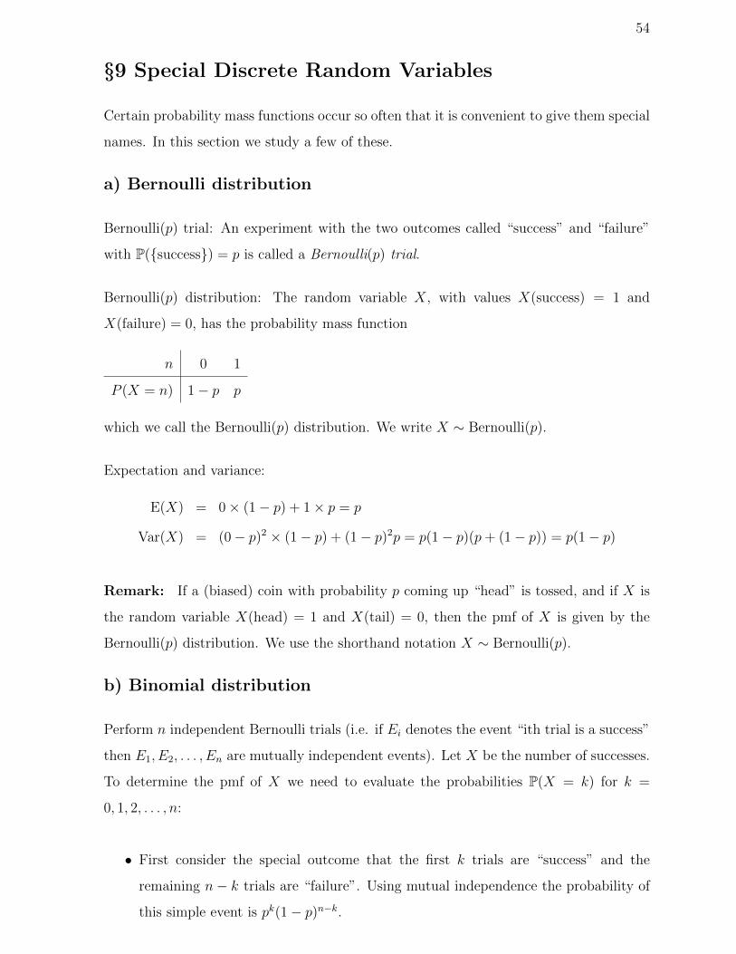
Bernoulli(p) trial: An experiment with the two outcomes called “success” and “failure”

with P(success) = p is called a Bernoulli(p) trial.

Bernoulli(p) distribution: The random variable X, with values X(success) = 1 and

X(failure) = 0, has the probability mass function

n 0 1

P (X = n) 1− p p

which we call the Bernoulli(p) distribution. We write X ∼ Bernoulli(p).

Expectation and variance:

E(X) = 0× (1− p) + 1× p = p

Var(X) = (0− p)2 × (1− p) + (1− p)2p = p(1− p)(p+ (1− p)) = p(1− p)

Remark: If a (biased) coin with probability p coming up “head” is tossed, and if X is

the random variable X(head) = 1 and X(tail) = 0, then the pmf of X is given by the

Bernoulli(p) distribution. We use the shorthand notation X ∼ Bernoulli(p).

b) Binomial distribution

Perform n independent Bernoulli trials (i.e. if Ei denotes the event “ith trial is a success”

then E1, E2, . . . , En are mutually independent events). Let X be the number of successes.

To determine the pmf of X we need to evaluate the probabilities P(X = k) for k =

0, 1, 2, . . . , n:

• First consider the special outcome that the first k trials are “success” and the

remaining n− k trials are “failure”. Using mutual independence the probability of

this simple event is pk(1− p)n−k.

55

• The event X = k contains(nk

)different outcomes with k “successes” and n − k

“failures” and each outcome occurs with the same probability pk(1− p)n−k.

Hence we obtain the pmf

P (X = k) =

(n

k

)pk(1− p)n−k .

We say X has the Binomial(n, p) (Bin(n, p)) distribution, X ∼ Bin(n, p).

Remark: Some useful identities:

• Binomial theorem

(a+ b)n =n∑k=0

(n

k

)akbn−k

• (n

k

)=

n!

k!(n− k)!=

n× (n− 1)!

k × (k − 1)!(n− k)!=n

k

(n− 1

k − 1

)

Expectation: Using the just mentioned identities

E(X) =n∑k=0

kP (X = k) =n∑k=1

k

(n

k

)pk(1− p)n−k =

n∑k=1

n

(n− 1

k − 1

)pk(1− p)n−k

= npn∑k=1

(n− 1

k − 1

)pk−1(1− p)n−k = np

n−1∑`=0

(n− 1

`

)p`(1− p)n−1−`

= np(p+ (1− p))n−1 = np .

Variance: Apply the aforementioned identity twice, i.e.,(n

k

)=n

k

(n− 1

k − 1

)=n

k

n− 1

k − 1

(n− 2

k − 2

).

Now

E(X2)− E(X) = E(X(X − 1)) =n∑k=0

k(k − 1)

(n

k

)pk(1− p)n−k

=n∑k=2

n(n− 1)

(n− 2

k − 2

)pk(1− p)n−k

= n(n− 1)p2n∑k=2

(n− 2

k − 2

)pk−2(1− p)n−k

= n(n− 1)p2n−2∑`=0

(n− 2

`

)p`(1− p)n−2−`

= n(n− 1)p2(p+ (1− p))n−2 = n(n− 1)p2 .

56

So

E(X2) = n(n− 1)p2 + E(X) = n(n− 1)p2 + np

and

Var(X) = E(X2)− [E(X)]2 = n(n− 1)p2 + np− (np)2 = −np2 + np = np(1− p) .

Remark: If a (biased) coin with probability p coming up “head” is tossed n times, and

if X denotes the random variable counting the numbers of heads then X ∼ Bin(n, p).

Example 9.1 A bag contains N balls M of which are red. You choose n balls with

replacement. Each random pick will result in a red ball with probability MN

and the outcome

of each pick is independent of all the others (i.e. we perform n independent Bernoulli trials

with p = M/N).

Let R denote (the random variable counting) the number of red balls. Then R ∼ Bin(n,M/N)

and

E(R) = nM

N, Var(R) = n

M

N

(1− M

N

).

c) Geometric distribution

Suppose we make an unlimited number of independent Bernoulli(p) trials and let T be the

number of trials up to and including the first success, see example 7.7. T = k consists of

a single event with k− 1 “failures”, each of which with probability 1− p, and one success

with probability p. Hence

P (T = k) = (1− p)k−1p

We say T has the geometric distribution, T ∼ Geom(p).

Remark: Some useful identities

• (see problem 23a), sheet 8)

∞∑k=1

kzk−1 = 1 + 2z + 3z2 + 4z3 + . . . =1

(1− z)2(∗)

57

• (see problem 23b), sheet 8)

∞∑k=1

k2zk−1 = 1 + 4z + 9z2 + 16z3 + . . . =2

(1− z)3− 1

(1− z)2(∗∗)

Expectation:

E(T ) =∞∑k=1

kP (T = k) =∞∑k=1

k(1− p)k−1p

= p(1 + 2(1− p) + 3(1− p)2 + 4(1− p)3 + . . .

)= p

1

[1− (1− p)]2using (*)

=1

p

Variance: Recall Var(T ) = E(T 2)− [E(T )]2

E(T 2) =∞∑k=1

k2P (T = k) =∞∑k=1

k2(1− p)k−1p

= p(1 + 4(1− p) + 9(1− p)2 + 16(1− p)3 + . . .

)= p

(2

[1− (1− p)]3− 1

[1− (1− p)]2

)using (**)

=2

p2− 1

p

Therefore

Var(T ) = E(T 2)− [E(T )]2 =2

p2− 1

p− 1

p2=

1− pp2

Example 9.2 A biased coin has probability p to show head. We toss the biased coin until

we see head for the first time. Let T denote the random variable counting the number of

coin tosses. T ∼ Geom(p) and P(T = k) is the probability that we perform exactly k coin

tosses.

P(T > k) is the probability that we perform more than k coin tosses (i.e. that the first k

tosses are all tail). Obviously (recall T > k and T = ` are events/sets)

(T > k) = (T = k + 1) ∪ (T = k + 2) ∪ (T = k + 3) ∪ . . .

58

and since all the simple events are disjoint

P(T > k) = P(T = k + 1) + P(T = k + 2) + P(T = k + 3) + . . .

= (1− p)kp+ (1− p)k+1p+ (1− p)k+2p+ . . .

= (1− p)kp(1 + (1− p) + (1− p)2 + (1− p)3 + . . .

)= (1− p)kp 1

1− (1− p)= (1− p)k .

The function k 7→ P(T > k) is called cumulative distribution function.

d) Poisson distribution

Consider a random variable X which takes values k = 0, 1, 2, 3, . . .. Denote by λ > 0 a

fixed positive real number. Define the pmf of the random variable X by

P(X = k) =λk

k!e−λ .

We say that X has the Poisson(λ) distribution, in short X ∼ Poisson(λ).

Remark:

• There is no simple way to illustrate the Poisson(λ) distribution. For instance, if

X counts the number of emissions in radioactive decay in a fixed time span then

X ∼ Poisson(λ).

• If 0 < λ ≤ 1 then the pmf P(X = k) is monotonic decreasing. If λ > 1 then the

pmf has a maximum at a finite value k > 0.

Remark: Some useful identity: the Taylor series of the exponential function

ex =∞∑k=0

xk

k!= 1 + x+

x2

2+x3

3!+ . . .

Using the Taylor series of the exponential function we have

∞∑k=0

P(X = k) = e−λ∞∑k=0

λk

k!= e−λeλ = 1

59

see lemma 7.1.

Expectation:

E(X) =∞∑k=0

kP(X = k) =∞∑k=1

kλk

k!e−λ = e−λ

∞∑k=1

λ× λk−1

(k − 1)!= λe−λ

∞∑`=0

λ`

`!= λ

Variance: To compute the variance consider again

E(X2)− E(X) = E(X(X − 1)) =∞∑k=0

k(k − 1)P(X = k) =∞∑k=2

k(k − 1)λk

k!e−λ

= e−λ∞∑k=2

λ2 × λk−2

(k − 2)!= λ2e−λ

∞∑`=0

λ`

`!= λ2

Hence E(X2) = λ2 + λ and

Var(X) = E(X2)− [E(X)]2 = λ2 + λ− λ2 = λ

e) Summary

range pmf P(X = k) E(X) Var(X)

X ∼ Bin(n, p) X = 0, 1, . . . , n

(n

k

)pk(1− p)n−k np np(1− p)

X ∼ Geom(p) X = 1, 2, 3, . . . (1− p)k−1p 1

p

1− pp2

X ∼ Poisson(λ) X = 0, 1, 2, . . .λk

k!e−λ λ λ

60

§10 Several Random Variables

Example 10.1 A bag contains 3 red balls, 2 blue balls, and 2 green balls. We pick 3 balls

at random. Let R denote the number of red balls, and B the number of blue balls. R and

B are two random variables defined on the same sample space.

In this section we will consider random variables defined on the same sample space.

Definition 10.1 Denote by X and Y two discrete random variable defined on the same

sample space. Assume X and Y take values (x1, x2, . . .) and (y1, y2, . . .), respectively. The

function

(xk, y`) 7→ P(X = xk ∩ Y = y`)

is called the joint probability mass function of X and Y .

Remark: Often one writes P(X = xk, Y = y`) instead of P(X = xk ∩ Y = y`).

Example 10.2 Consider the experiment of example 10.1. Use unordered sampling with-

out replacement, section 3c, to work out probabilities.

|S| =(73

)= 35. To work out, e.g., P(R = 1, B = 1) recall that we sample a red ball from

a subset of 3, a blue ball from a subset of 2 and a green ball from a subset of 2 giving(31

)(21

)(21

)possibilities. Hence P(R = 1, B = 1) = 12/35. The other probabilities can be

worked out in the same way and are summarised in a table.

@@@@@

B

R0 1 2 3

0 0 3/35 6/35 1/35

1 2/35 12/35 6/35 0

2 2/35 3/35 0 0

The joint pmf satisfies (see as well lemma 7.1)∑k

∑`

P(X = xk, Y = y`) = 1 .

61

The joint pmf and the pmf for X and Y , the so called marginal distributions, are related

by

P(X = xk) =∑`

P(X = xk, Y = y`), P(Y = y`) =∑k

P(X = xk, Y = y`) .

Example 10.3 Consider the joint pmf of example 10.2.

Clearly the entries in the table add up to one.

Marginal distributions: column sum

k 0 1 2 3

P(R = k) 4/35 18/35 12/35 1/35

row sum

` 0 1 2

P(B = `) 10/35 20/35 5/35

Expectations:

E(R) =3∑

k=0

kP(R = k) =0× 4 + 1× 18 + 2× 12 + 3× 1

35=

9

7

E(B) =2∑`=0

`P(B = `) =0× 10 + 1× 20 + 2× 5

35=

6

7

Expectations are defined and can be computed in the obvious way (see definition 8.1).

Definition 10.2 If g(X, Y ) is a (real valued) function of the two discrete random vari-

ables X and Y then

E(g(X, Y )) =∑k

∑`

g(xk, y`)P(X = xk, Y = y`)

defines the expectation of g(X, Y ).

Example 10.4 Consider the experiment in example 10.1. R + B is the number of red

and blue balls, R × B is the product of the number of red and blue balls. Using the joint

probability mass function of example 10.2 we have

E(R+B) = 0×0 + 1×(

3

35+

2

35

)+ 2×

(6

35+

12

35+

2

35

)+ 3×

(1

35+

6

35+

3

35

)=

15

7.

62

Note that E(R +B) = E(R) + E(B). Furthermore

E(R×B) = 1× 12

35+ 2×

(6

35+

3

35

)=

6

7.

Note that E(R×B) 6= E(R)× E(B).

Theorem 10.1 If X and Y are discrete random variables then

E(X + Y ) = E(X) + E(Y ) .

Proof:

E(X + Y ) =∑k

∑`

(xk + y`)P(X = xk, Y = y`)

=∑k

∑`

xkP(X = xk, Y = y`) +∑k

∑`

y`P(X = xk, Y = y`)

=∑k

xk

(∑`

P(X = xk, Y = y`)

)+∑`

y`

(∑k

P(X = xk, Y = y`)

)=

∑k

xkP(X = xk) +∑`

y`P(Y = y`) = E(X) + E(Y )

.

Applying theorem 10.1 repeatedly, that means, E(X + Y + Z) = E(X + Y ) + E(Z) =

E(X) + E(Y ) + E(Z) and using the properties of expectations, proposition 8.2iii), we

arrive at

Corollary 10.1 (Linearity of expectation) If X1, X2, . . . , Xn are discrete random vari-

ables and c1, c2, . . . , cn real valued constants then

E(c1X1 + c2X2 + . . .+ cnXn) = c1E(X1) + c2E(X2) + . . .+ cnE(Xn) .

Example 10.5 Consider the sample space of a Bernoulli(p) trial and define n random

variables X1, X2, . . . , Xn such that Xi(success) = 1 and Xi(failure) = 0, see section 9a.

Hence E(X1) = E(X2) = . . .E(Xn) = p. Consider the random variable X = X1 + X2 +

. . .+Xn. Then by corollary 10.1 (see as well section 9b)

E(X) = E(X1 +X2 + . . .+Xn) = E(X1) + E(X2) + . . .+ E(Xn) = np .

63

Definition 10.3 Two random variables are independent if for all xk and y` we have

P(X = xk, Y = y`) = P(X = xk)P(Y = y`) .

Equivalently, the random variables X and Y are independent if for all xk, y`, the events

X = xk and Y = y` are independent.

The random variables X1, X2, . . . , Xn are independent if for all x1, x2, . . . , xn we have

P(X1 = x1, X2 = x2, . . . , Xn = xn) = P(X1 = x1)P(X2 = x2) . . .P(Xn = xn).

Example 10.6 The random variables R and B in the experiment of example 10.1 are

not independent.

For instance, using the probabilities in example 10.2 and example 10.3

12

35= P(R = 1, B = 1) 6= P(R = 1)P(B = 1) =

18

35× 20

35.

Remark: Some useful identity

(a1 + a2)(b1 + b2) = a1b1 + a1b2 + a2b1 + a2b2

i.e. (2∑

k=1

ak

)(2∑`=1

b`

)=

2∑k,`=1

akb`

The relation holds for general sums(∑k

ak

)(∑`

b`

)=∑k,`

akb`

Theorem 10.2 If X and Y are independent discrete random variables then:

i) E(XY ) = E(X)E(Y ),

ii) Var(X + Y ) = Var(X) + Var(Y ).

Proof:

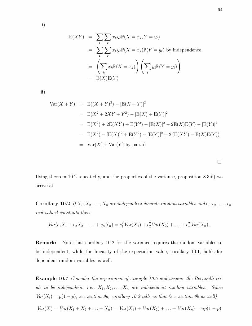
64

i)

E(XY ) =∑k

∑`

xky`P(X = xk, Y = y`)

=∑k

∑`

xky`P(X = xk)P(Y = y`) by independence

=

(∑k

xkP(X = xk)

)(∑`

y`P(Y = y`)

)= E(X)E(Y )

ii)

Var(X + Y ) = E((X + Y )2)− [E(X + Y )]2

= E(X2 + 2XY + Y 2)− [E(X) + E(Y )]2

= E(X2) + 2E(XY ) + E(Y 2)− [E(X)]2 − 2E(X)E(Y )− [E(Y )]2

= E(X2)− [E(X)]2 + E(Y 2)− [E(Y )]2 + 2 (E(XY )− E(X)E(Y ))

= Var(X) + Var(Y ) by part i)

.

Using theorem 10.2 repeatedly, and the properties of the variance, proposition 8.3iii) we

arrive at

Corollary 10.2 If X1, X2, . . . , Xn are independent discrete random variables and c1, c2, . . . , cn

real valued constants then

Var(c1X1 + c2X2 + . . .+ cnXn) = c21Var(X1) + c22Var(X2) + . . .+ c2nVar(Xn) .

Remark: Note that corollary 10.2 for the variance requires the random variables to

be independent, while the linearity of the expectation value, corollary 10.1, holds for

dependent random variables as well.

Example 10.7 Consider the experiment of example 10.5 and assume the Bernoulli tri-

als to be independent, i.e., X1, X2, . . . , Xn are independent random variables. Since

Var(Xi) = p(1− p), see section 9a, corollary 10.2 tells us that (see section 9b as well)

Var(X) = Var(X1 +X2 + . . .+Xn) = Var(X1) + Var(X2) + . . .+ Var(Xn) = np(1− p)

65

§11 Covariance and Conditional Expectation

Let us introduce some quantity which tell us by “how much” two random variables depend

on each other.

Definition 11.1 If X and Y are discrete random variables the covariance of X and Y

is defined to be

Cov(X, Y ) = E(XY )− E(X)E(Y ).

The correlation coefficient of X and Y is defined to be

corr(X, Y ) =Cov(X, Y )√

Var(X)Var(Y ).

Remark:

• If X and Y are independent, definition 10.3, then according to theorem 10.2 we

have Cov(X, Y ) = corr(X, Y ) = 0. But: Cov(X, Y ) = 0 does not necessarily imply

X and Y to be independent.

• If X and Y have the tendency to be either both positive or both being negative

(to be precise: X − E(X) and Y − E(Y ) both being positive/negative) then the

covariance and the correlation coefficient will be positive. If there is a tendency for

X being positive and Y being negative, or vice versa, then the covariance and the

correlation coefficient will be negative.

• The correlation coefficient obeys −1 ≤ corr(X, Y ) ≤ 1 (see problem 32c, sheet 11).

Example 11.1 Consider the experiment of example 10.1. Examples 10.3 and 10.4 tell

us that

Cor(R,B) = E(RB)− E(R)E(B) =6

7− 6

7× 9

7= −12

49

The covariance is negative, that makes sense. Having more red balls (on average) makes

it likely to have fewer blue balls (on average).

Proposition 11.1 (Properties of covariance and correlation coefficient) If X and

Y are random variables then:

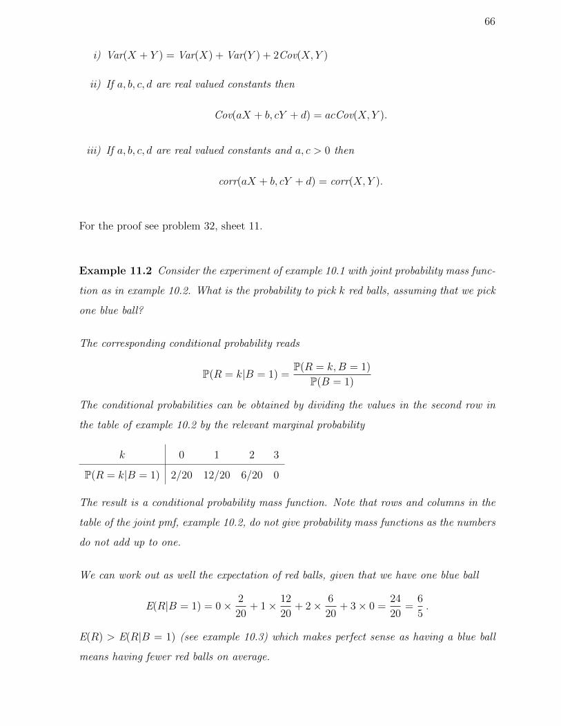
66

i) Var(X + Y ) = Var(X) + Var(Y ) + 2Cov(X, Y )

ii) If a, b, c, d are real valued constants then

Cov(aX + b, cY + d) = acCov(X, Y ).

iii) If a, b, c, d are real valued constants and a, c > 0 then

corr(aX + b, cY + d) = corr(X, Y ).

For the proof see problem 32, sheet 11.

Example 11.2 Consider the experiment of example 10.1 with joint probability mass func-

tion as in example 10.2. What is the probability to pick k red balls, assuming that we pick

one blue ball?

The corresponding conditional probability reads

P(R = k|B = 1) =P(R = k,B = 1)

P(B = 1)

The conditional probabilities can be obtained by dividing the values in the second row in

the table of example 10.2 by the relevant marginal probability

k 0 1 2 3

P(R = k|B = 1) 2/20 12/20 6/20 0

The result is a conditional probability mass function. Note that rows and columns in the

table of the joint pmf, example 10.2, do not give probability mass functions as the numbers

do not add up to one.

We can work out as well the expectation of red balls, given that we have one blue ball

E(R|B = 1) = 0× 2

20+ 1× 12

20+ 2× 6

20+ 3× 0 =

24

20=

6

5.

E(R) > E(R|B = 1) (see example 10.3) which makes perfect sense as having a blue ball

means having fewer red balls on average.

67

Definition 11.2 Let X be a discrete random variable and A is an event with P(A) > 0.

The conditional probability

P(X = xk|A) =P(X = xk ∩ A)

P(A).

defines the probability mass function of X given A. The corresponding expectation

E(X|A) =∑k

xkP(X = xk|A)

is called the conditional expectation.

Remark: One may consider X|A (“random variable X given an event A”) as a random

variable with pmf being given by definition 11.2

Example 11.3 A standard fair die is rolled twice. Let X be the number showing on the

first roll and A be the event “at least one odd number is rolled”. Find the probability mass

function of X|A.

We have that P(A) = 3/4.

Consider a fixed value k. k may be even or odd.

If k is odd then the event (X = k)∩A (“first roll k/odd and at least one odd number”) is

equal to X = k (“first roll k/odd”). Hence

P(X = k|A) =P(X = k ∩ A)

P(A)=

P(X = k)

P(A)=

1/6

3/4=

2

9.

If k is even then the event X = k ∩ A (“first roll k/even and at least one odd number”)

is equal to the event “first roll k/even and second roll odd”) so that (using independence

of rolls) P (X = k ∩ A) = P(X = k)× 1/2 = 1/6× 1/2 and

P(X = k|A) =P(X = k ∩ A)

P(A)=

1/6× 1/2

3/4=

1

9.

It follows that the conditional pmf of X|A is

k 1 2 3 4 5 6

P(X = k|A) 2/9 1/9 2/9 1/9 2/9 1/9

In addition

E(X|A) =2 + 2 + 6 + 4 + 10 + 6

9=

10

3.

68

The following statement can be considered to be a special case of theorem 6.1

Theorem 11.1 Denote by A1, A2, . . . , An a partition of S (that is the sets are pairwise

disjoint and their union is S) with P(Ai) > 0 for all i,. If X is a discreet random variable

then

E(X) =n∑i=1

E(X|Ai)P(Ai) .

Proof: Apply the Theorem of Total Probability, theorem 6.1, for the event X = xk with

the partition A1, . . . , An

P(X = xk) =n∑i=1

P(X = xk|Ai)P(Ai) .

By definition

E(X) =∑k

xkP(X = xk).

so

E(X) =∑k

xk

n∑i=1

P(X = xk|Ai)P(Ai) =n∑i=1

∑k

xkP(X = xk|Ai)P(Ai)

=n∑i=1

E(X|Ai)P(Ai) .

.

Example 11.4 We toss a fair coin. If the coin comes up heads we roll a standard 6-sided

die. If it comes up tails we roll a standard 4-sided die (with sides numbered 1, 2, 3, 4). Let

X be the number we roll. Find its expectation.

Let H be the event “coin shows head”. Clearly H,Hc is a partition and P(H) = P(Hc) =

1/2 (as the coin is fair).

X|H is the (random variable) number shown by the die given the coins shows head, i.e.,

the number shown by the 6 sided die. Clearly its expectation reads

E(X|H) =1 + 2 + 3 + 4 + 5 + 6

6=

7

2.

X|Hc is the (random variable) number shown by the die given the coin shows tail, i.e.,

the number shown by the 4 sided die. Clearly

E(X|Hc) =1 + 2 + 3 + 4

4=

5

2.

69

Theorem 11.1 with the partition H,Hc gives

E(X) = P(X|H)P(H) + P(X|Hc)P(Hc) =7

2× 1

2+

5

2× 1

2= 3

Example 11.5 (simple random walk) Consider an infinite one dimensional lattice where

sites are labelled by integers. Consider a walker on this lattice and let Xt denote the

position of the walker at discrete time t where t = 0, 1, 2, 3, . . ..

At time t = 0 the walker is at site 0, i.e., X0 = 0. At each time step the walker moves

with probability 1/2 to either the site left or right of their current position, i.e., if Xt−1 = `

then Xt = `+1 with probability 1/2 and Xt = `−1 with probability 1/2. Written in terms

of conditional probabilities P(Xt = `+ 1|Xt−1 = `) = 1/2, P(Xt = `− 1|Xt−1 = `) = 1/2,

and P(Xt = k|Xt−1 = `) = 0 if k 6= `± 1.

Compute the expectation of Xt.

Using theorem 11.1 with the partition A` = (Xt−1 = `) we have

E(Xt) =∞∑

`=−∞

E(Xt|Xt−1 = `)P(Xt−1 = `) .

Definition 11.2 tells us

E(Xt|Xt−1 = `) =∞∑

k=−∞

kP(Xt = k|Xt−1 = `) =1

2(`+ 1) +

1

2(`− 1) = ` .

Hence

E(Xt) =∞∑

`=−∞

`P(Xt−1 = `) = E(Xt−1)

Therefore E(Xt) = E(X0) = 0 (i.e. on average the walker does not move).