introduction to optimization and multidisciplinary...

von Karman Institute for Fluid Dynamics

Lecture Series 2016-03

INTRODUCTION TO OPTIMIZATION AND MULTIDISCIPLINARY DESIGN

May 23-27, 2016

THEORETICAL BACKGROUND FOR AERODYNAMIC SHAPE OPTIMIZATION

J. C. Vassberg1 & A. Jameson2 1Boeing Commercial Airplanes, USA

2Stanford University, USA

Theoretical Background for

Aerodynamic Shape Optimization

John C. Vassberg ∗

Advanced Concepts Design CenterBoeing Commercial AirplanesLong Beach, CA 90846, USA

Antony Jameson †

Department of Aeronautics & AstronauticsStanford University

Stanford, CA 94305-3030, USA

Von Karman InstituteBrussels, Belgium

23 May, 2016

Nomenclature

A Hessian Matrix / Operator

a Integrand of Integral Hessian Operator

C Constant; Constrain equation

E Error of Discretization

F Integrand of Cost Function

G Gradient of Cost Function

G Implicitly-Smoothed Gradient

g Acceleration due to Gravity ≃ 32.2 ft

sec2

GRMS Root-Mean-Square of Gradient Vector

H Estimate of Inverse Hessian Matrix

I Objective or Cost Function

IR Discrete I based on Rectangle Rule

ITERS Iterations needed for 10−6 Reduction

i Matrix Row Index

j Spatial Index; Matrix Column Index

k Generic Index

K Upper Limit of Generic Index k

L Lagrangian Dual Cost Function

N Number of Design Variables

n Iteration Index

NMESH Number of Multigrid Levels

NX Number of Mesh Intervals

P Multigrid Forcing Function

P Error Vector of Rank-One Scheme

Q Multigrid Transfer Operator

STEP Input Parameter Similar to CFL Number

Surplus ICR − ID

R

S Geodesic Path Length

s Arch Length

T Total Time; Multigrid Transfer Operator

t Parametric Variable; Time

v Velocity

X Design Variable

x Independent Spatial Variable

X Design Space Vector [X, Y, Z]T

Y Design Variable

y Design Variable

Y ERR L2 Norm of y − yexact vector

Z Design Variable

α Tridiagonal Coefficient of Implicit Scheme

β Coefficient of Parabolic Term

γ Recombination Coefficients

ǫ Implicit Smoothing Parameter

λ Time-Step Parameter

µ Lagrange Multiplier

ξ Free Variable

π 3.141592654...

∞ Infinity

δ∗ First Variation of

∆∗ Change in

∇∗ Gradient of

∂∗ Partial of

O(∗) Order of

(∗)T Matrix Transpose of

(∗)−1 Inverse Matrix of

∗′ First Derivative of, ∂

∂x

∗′′ Second Derivative of, ∂2

∂x2

∗Boeing Technical Fellow†T. V. Jones Professor of Engineering

Copyright c© 2016 by Vassberg & Jameson.

Published by the VKI with permission.

Vassberg & Jameson, VKI Lecture-I, Brussels, Belgium, 23 May, 2016 1 of 45

1 Introduction

This is the first of three lectures prepared by the authors for the von Karman Institute that deal withthe subject of aerodynamic shape optimization. In this lecture we introduce some theoretical backgroundon optimization techniques commonly used in the industry, apply some of the approaches to a couple ofvery simple model problems, and compare the results of these schemes. We also discuss their merits anddefficiencies as they relate to the class of aerodynamic shape optimization problems the authors deal with ona daily basis. In the second lecture, we provide a set of sample applications, while the third lecture is focusedon parameterization of the design space. However, before we continue with the simple model problems ofthis lecture, let’s first review some properties of the aerodynamic shape optimization studies the authors areregularly concerned with.

In an airplane design environment, there is no need for an optimization based purely on the aerodynamicsof the aircraft. The driving force behind (almost) every design change is related to how the modificationimproves the vehicle, not how it enhances any one of the many disciplines that comprise the design. Andalthough we focus our lectures on the aerodynamics of an airplane, we also include the means by which otherdisciplines are linked into and affect the aerodynamic shape optimization subtask; these will be addressedin detail in the second lecture. Another characteristic of the problems we typically (but not always) work,is that the baseline configuration is itself within 1-2% of what may be possible, given the set of constraintsthat we are asked to satisfy. This is certainly true for commercial transport jet aircraft whose designs havebeen constantly evolving for the past half century or more. This class of problems is much more demandingthan those in which the baseline is far from the optimum design. Frequently, it is easier to show a 25%improvement relative to a baseline that is 30% off optimum than it is to realize a 1% gain on a startingconfiguration that only has 2% to give.

Quite often the problem is very constrained; this is the case when the shape change is required to be aretrofitable modification that can be applied to aircraft already in service. Occasionally, we can begin witha clean slate, such as in the design of an all-new airplane. And the problems cover the full spectrum ofstudies in between these two extremes. Let’s note a couple of items about this setting. First, in order torealize a true improvement to the baseline configuration, a high-fidelity and very accurate computationalfluid dynamics (CFD) method must be employed to provide the aerodynamic metrics of lift, drag, pitchingmoment, spanload, etc. Even with this, measures should be taken to estimate the possible error band of thefinal analyses: this discussion is beyond the scope of these lectures. The second item to consider is related tothe definition of the design space. A common practice is to use a set of basis functions which either describethe absolute shape of the geometry, or define a perturbation relative to the baseline configuration. In orderto realize an improvement to the baseline shape, the design space should not be artificially constrained bythe choice of the set of basis functions. This can be accomplished with either a small set of very-well-chosenbasis functions, or with a large set of reasonably-chosen basis functions. The former approach places theburden on the user to establish an adequate design space; the latter approach places the burden on theoptimization software to economically accommodate problems with large degrees of freedom. Over the pasttwo decades, the authors have focused on solving the problem of aerodynamic shape optimization utilizinga design space of very large dimension. The interested reader can find copious examples of the alternativeapproaches throughout the literature.

With some understanding of where we are headed, let’s now return to the simple model problems includedherein, review various aspects of the optimization process, and discuss how these relate to the aerodynamicshape optimization problem at hand. The first model problem introduces some of the basics; the second oneis a classic example in mathematical history.

2 The Spider & The Fly

In our first model problem, we will discuss how to set up a design space, how to numerically approximate thegradient and the Hessian matrix, how to impose active constraints, and how to navigate this design spacefrom an initial state towards a local optimum using gradient-based search methods. We will also talk aboutsome traps to avoid when setting up a problem of optimization.

The original spider and fly problem was first introduced by Dudeney [1] in 1903. In our version of thespider-fly problem, we have a wooden block with dimensions of 4 in wide, by 4 in tall, by 12 in long; thebottom of this block is resting on a solid flat surface. See Figure 1. On one of the square ends sits a spider,


located 1 in from the top and centered left-to-right. On the opposite side a fly is trapped in the spider’s web;the fly is located 1 in from the bottom and centered left-to-right. The spider considers the path where hewould initially travel 1 in straight up to the top, then 12 in axially across the top face, then 3 in downwardto the fly; the length of this path is 16 in. This path represents a local optimum path.

As it turns out, the spider was a mathematician in a former lifetime, so he wonders if this is the globalminimum-length path possible. In order to solve this enigma and determine the true geodesic, the spidersets up a problem of optimization. To cast this optimization problem into a mathematical formulation, thespider must some how constrain his motion to the surface of the wooden block, and furthermore, he knowshe cannot traverse the bottom side of the block as it is resting on the solid flat surface. It is clear that theaforementioned 16 in path is a local optimum, and due to the symmetry of the problem, there are reallyonly two other types of paths that need to be studied. In one type, the spider moves laterally 2+ in towardthe right/left side of the block, then 12+ in across that side towards the back, then 2+ in to the trapped fly.Here, the length of any path of this type is definitely in excess of 16 in, and therefore the global optimumcannot be a path of this type. The remaining path type allows the spider to move upward 1+ in to the top ofthe block, continue diagonally towards the right/left side, then diagonally across and downward towards theback face, and finally 2+ in to the fly. See Figure 2. It is not immediately obvious that the local optimum ofthis path type cannot also be the global optimum. Hence, the spider must investigate further to determinethe geodesic from his position to that of the fly’s.

Design Space Set Up

To set up the design space for this problem, the spider adopts a cartesian coordinate system aligned with thewooden block such that the origin coincides with the front-lower-left corner of the block. The x coordinatemeasures positive to the right, the y coordinate measures positive along the long side of the block away fromthe front face, and the z coordinate measures positive upward in the vertical direction. In this coordinatesystem, the spider’s initial position on the front face is (XS, Y S, ZS) = (2, 0, 3), and the fly is trapped onthe back face at (XF, Y F, ZF ) = (2, 12, 1).

The path type to optimize can be partitioned into four segments, corresponding to the four block facesto be traversed. The first segment is described by end points (2, 0, 3) and (X, 0, 4). The second segment’send points are (X, 0, 4) and (4, Y, 4). The third, (4, Y, 4) and (4, 12, Z). The fourth, (4, 12, Z) and (2, 12, 1).Hence, the complete path can be described as the piecewise linear curve that connects (2, 0, 3), (X, 0, 4),(4, Y, 4), (4, 12, Z), and (2, 12, 1). In this design space, there are precisely three design variables (X, Y, Z).Further, the design space is constrained by the inequalities:

0 ≤ X ≤ 4,0 ≤ Y ≤ 12,0 ≤ Z ≤ 4.

(1)

Hence, the design space as defined in this problem is constrained to the interior of the wooden block. Whilethese constraints facilitate limiting the search for the optimium, once we find the optimum path, it willbecome obvious that these are non-active constraints. So we will follow up this problem with an addendumproblem which introduces another constraint on the path to illustrate how one can handle constraints thatmay or may not become active at the constrained minimum.

Cost Function

The length of each segment is given as:

S1 =[

1 + (X − 2)2]

1

2 ,

S2 =[

(X − 4)2 + Y 2]

1

2 ,

S3 =[

(Y − 12)2 + (Z − 4)2]

1

2 ,

S4 =[

(Z − 1)2 + 4]

1

2 .

(2)

The total path length (or objective/cost function) is defined as:

I ≡ S = S1 + S2 + S3 + S4. (3)


The statement of optimization is to minimize I subject to the constraints of Eqn (1). Note that Eqn (3) isnot a quadratic equation. Furthermore, this cost function is not equivalent to summing the squares of theline segment lengths, which is a quadratic equation. So, always be careful when defining your cost function.I emphasize this point, as this question has been asked in the past and argued with conviction.

There are many ways in which one can proceed to solve this problem of optimization. For example, oneapproach is to use evolution theory, where a population of random guesses of (X, Y, Z)i is evaluated for theirassociated set of cost-function values, Ii. This establishes a generation of information which can be usedto coerse subsequent generations towards the optimum location within the design space. An improvementto basic evolution theory is the Genetic Algorithm (GA). GAs attempt to speed the evolution process bycombining the genes of promising pairs from one generation to procreate the next. GAs also allow somefraction of mutations to occur in order to improve the chance of finding a global optimum. However ingeneral, this is not guaranteed. These methods are relatively easy to set up and program as they do notrequire any gradient information, and in fact may be the best choice if the cost function does not smoothlyvary throughout the design space. Unfortunately, they can be computationally very expensive, even for aproblem with a modest number of design variables. Nonetheless, solving the spider-fly problem with evolutionmethods can be entertaining, and we recommend it to the ambitious student as a follow-up exercise to thislecture.

Gradient-Based Optimization

Let’s now consider gradient-based optimization techniques. These optimization methods use derivatives ofthe objective function with respect to the design space to navigate the design space from an initial state toa local optimum. These techniques include steepest descent, Newton methods, and quasi-Newton methods,amoung others.

In the case of the spider-fly problem, the exact derivatives are easily found. However, in general thisis not usually the case for most large-scale problems of interest, so one may have to resort to utilizing anapproximate derivative. We will study both, and introduce a couple of basic methods that one can use toapproximate the gradient of a cost function.

Exact Gradient

Let’s return to the definition of the cost function given by Eqns (2-3). In this simple example problem it isstraightforward to derive the first and second derivatives of the cost function. Hence, the first variation ofthe cost function is:

δI = IXδX + IY δY + IZδZ ≡ G δX (4)

where G is the gradient vector, X is the design space vector, and the partial derivatives with respect to thedesign space are given as:

IX = (X−2)S1

+ (X−4)S2

,

IY = YS2

+ (Y −12)S3

,

IZ = (Z−4)S3

+ (Z−1)S4

.

(5)

Exact Hessian

Now find the Hessian matrix (second derivatives) for this problem; it will be needed to navigate the designspace with a Newton iteration. The Hessian matrix is:

A =

IXX IY X IZX

IXY IY Y IZY

IXZ IY Z IZZ

(6)


where,

IXX = 1S3

1

+ Y 2

S3

2

IXY = IY X = (4−X)YS3

2

IXZ = IZX = 0

IY Y = (X−4)2

S3

2

+ (Z−4)2

S3

3

IY Z = IZY = (Y −12)(4−Z)S3

3

IZZ = (Y −12)2

S3

3

+ 4S3

4

(7)

Approximate Gradient by Finite Differences

One can approximate the gradient by finite differences, where the amplitude of each design variable isindependently perturbed by a small delta from the current state and the cost function reevaluated. Ingeneral, this requires N + 1 function evaluations to approximate the gradient, where N is the number ofdesign variables. (N is also referred to as the number of degrees of freedom, or as the dimension of the designspace.)

Consider the Taylor series expansion of a function f .

f(x + ∆x) = f(x) + ∆x fx(x) +∆x2

2fxx(x) + . . . +

∆xn

n!fn(x) + . . . (8)

A first-order accurate approximation of fx(x) can be determined from Eqn (8) with a forward differencing.

fx(x) ≃ f(x + ∆x) − f(x)

∆x. (9)

Using Eqn (9), let’s approximate IX of Eqn (5).

IX ≃ I(X + h, Y, Z) − I(X, Y, Z)

h(10)

Where h = ∆x is a small perturbation of the X coordinate. Using Eqn (10) with h = 10−3 at (X, Y, Z) =(2, 6, 2) gives IX ≃ −0.31565661, an error of about 0.1%. The exact value of IX at this location is − 2√

40≃

−0.31622777. In exact mathematics, the accuracy of IX improves as h → 0. However, if we evaluate theapproximation of this derivative with various values of h using finite-precision mathematics, one will quicklyfind that as h gets really small, the stability of this evaluation will eventually degrade. For example at(X, Y, Z) = (2, 6, 2) and using 64-bit precision, the finite-difference estimate of IX improves with decreasingh until h < 10−7, as shown below in Table 1. However at this point, the trend reverses and the errorof IX begins to grow with decreasing h. And remember, this is a simple cost function. A cost functionfor aerodynamic shape optimization is typically related to the computed drag of a design. Computing ahigh-precision value for drag can be quite costly, and in this context, finding an appropriate value of h foreach design variable can become problematic. In practice, using a second-order accurate finite differencingof the function not only doubles the cost of the gradient, it typically does not solve the stability issue offinite-precision computations.

Approximate Gradient by Complex Variables

Another approach to approximating the gradient is now presented which, as it turns out, is much more stablethan finite differences. In general, the computational cost of this technique also scales with O(N) functionevaluations.

Let’s revisit the Taylor series of Eqn (8). This expansion also holds true for complex functions of complexvariables. With this in mind, let’s now consider an imaginary perturbation of X , where ∆x = ih. If we take


log10(Error IX)log10(h) Finite Difference Complex Variable

-1 -1.244 -4.449-2 -2.243 -6.449-3 -3.243 -8.449-4 -4.243 -10.449-5 -5.243 -12.449-6 -6.244 -14.449-7 -7.192 -16.256-8 -6.778 -16.256-9 -5.977 -16.256-10 -4.768 -16.256

00

-2

-4

-6

-8

-10

-12

-14

-16

-18

00-1-2-3-4-5-6-7-8-9-10-11

Finite Difference vs Complex Variables

log10 ( h )

log1

0 (

Err

or[I

x] )

Finite Difference

Complex Variables

Table 1: Stability of Finite-Difference and Complex-Variable Methods.

the imaginary part of the expansion of f(x + ih), we get a second-order accurate approximation of fx, asgiven below.

fx(x) ≃ Im[f(x + ih)]

h. (11)

Now we can approximate IX using Eqn (11).

IX ≃ Im[I(X + ih, Y, Z)]

h(12)

Eqn (12) for all h ≤ 10−3 at (X, Y, Z) = (2, 6, 2) gives IX ≃ −0.31622777, which is identical to the exactvalue of this derivative to 8 significant digits. Table 1 illustrates the improved accuracy and stability of usingcomplex variables relative to using finite differences to approximate the gradient of a function. Note thatwhile the finite-difference error reverses its trend at h ≤ 10−7, the complex-variable estimates level out.

Additional information on the complex-variable method for approximating gradients for the Navier-Stokesequations can be found in Anderson et. al. [2].

Steepest Descent

One can use the gradient to establish a steepest descent trajectory of the cost function through the designspace. This trajectory begins with the initial state (baseline) and ends at a local minimum. From Eqn (4) itcan be seen that a reduction in the cost function is realized if a sufficiently small step is taken in the negativegradient direction, and a local minimum is found when the magnitude of the gradient vanishes. Accordingly,we can iteratively update the value of the design variables in the following manner.

Xn+1 = Xn + δXn, (13)

where n is the iterative step number, and

δXn = −λG. (14)

Here, λ > 0 is a step-size parameter. Thus,

δIn = G δXn = −λG2 ≤ 0. (15)

In order to initialize the trajectory search for the spider-fly problem, we arbitrarily select the center of theallowable design space as our baseline path. This corresponds to the following initial state for the designspace vector, X 0, the gradient vector, G0, and the Hessian matrix, A0. Note that for this arbitrarily chosenstate, the objective function, I0, is already less than that of the local-minimum path of Figure 1; this is


nothing more than a coincidence.

X 0 =

262

, G0 =

−2√40

0.0( −3√

40+ 1√

5)

≈

−0.316230.0

−0.02713

,

A0 ≈

1.14230 0.04743 0.00.04743 0.03162 −0.04743

0.0 −0.04743 0.50007

,

(16)

with

I0 = (1 + 2√

40 +√

5) ≈ 15.88518.

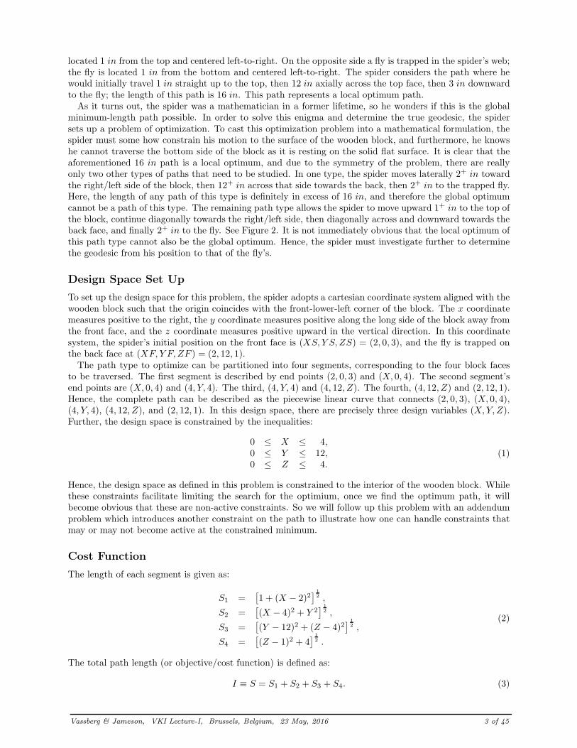
In a steepest descent procedure, the value of the free parameter λ is usually limited by the stability of theiterative process. We will discuss this further in our second model problem. Through some experimentation,a value of λ = 1.885 yields about the fastest convergence to the optimum state for the spider-fly problem.Using 64-bit mathematical operations, the exact minimum-distance path is found within machine-level-zeroin 295 iterations. The convergence of the gradient is shown in Figure 3. Here, the magnitude of the gradienthas been reduced more than 7.5 orders of magnitude. Figure 4 provides the trajectory of the optimizationprocess through the design space from start to finish. Notice the top view of this trajectory. Here onecan see the high-frequency zig-zag nature of this navigation, but it appears that the general trend of thetrajectory is correct. If the high-frequency behavior could be filtered and the low-frequency trend amplified,then convergence to the optimum could be accelerated. Such a technique will be addressed in our secondmodel problem of this lecture.

Newton Iteration

Now let us solve this optimization problem with a Newton iteration. To develop a Newton iteration, simplyreplace the variation of the design variables of Eqn (14) with

δXn = −A−1G = −HG, (17)

where H = A−1 is the inverse of the Hessian matrix of Eqns (6-7). Using this approach, the exact solution tomachine-level-zero is found in just 3 steps. Figure 5 provides the convergence of the gradient, and as expected,this convergence has a quadratic behavior. Figure 6 illustrates the corresponding navigation through thedesign space. Data from the Newton iteration are also given in Table 2.

In this model problem, the superior performance of the Newton iteration over that of the steepest descentmethod may lead one to abandon steepest descent in favor of an approach that utilizes the Hessian. However,let’s investigate the requirements of a Newton method in more depth. First, the construction of the Hessianmatrix can cost O(N) times that of the gradient, unless the Hessian happens to be a sparse matrix. In the caseof the spider-fly problem, this additional computational work trades very favorably (i.e., 3(1 + 3) << 295).However, when N is moderately large, this may no longer be the case. A second issue is that the terms ofthe Hessian matrix may not be explicitly available, and in fact this is usually the case for aerodynamic shapeoptimization problems.

n Xn Y n Zn In

0 2.000000 6.000000 2.000000 15.885181 2.319023 4.984009 1.641696 15.811672 2.333268 4.999744 1.666556 15.811393 2.333333 5.000000 1.666667 15.81139

Table 2: Convergence of Newton Iteration on the Spider-Fly Problem.


Quasi-Newton Methods

To consider this scenario, let’s assume that neither the Hessian matrix, A, or its inverse, H , are readilyavailable for the spider-fly problem. Under this circumstance, a quasi-Newton method can be employed.For the purpose of providing this case as a training exercise, we will document in detail the results of anapplication of a Rank-1 (R1) quasi-Newton iteration to the spider-fly problem. In this approach, the inverseof the Hessian matrix, H , is approximated and updated concurrently with the trajectory search. The Rank-1updates of H are given by the following relationship.

Hn+1 = Hn +(Pn)(Pn)T

(Pn)T δGn, (18)

whereδGn = Gn+1 − Gn

andPn = δXn − HnδGn.

Here, n is the iteration index, with n = 0 representing the initial state, and H0 being initialized as theidentity matrix. P is an error vector of the Rank-1 approximation of the Hessian. In the case of the spider-flyproblem, Hn is a 3x3 matrix, and δXn, δGn & Pn are 3-dimensional vectors. Note that [(Pn)(Pn)T ] is a 3x3matrix, and [(Pn)T δGn] is a scalar inner product. The numerical results of the R1 trajectory are illustratedin Figures 7-8, and tabulated in Table 3. Although it takes 6 to 7 iterations before the Hessian inverse issufficiently approximated, the R1 iterations eventually exhibit quadratic convergence. Close inspection ofTable 3 reveals some trends worth noting. Recall that vector Pn is a measure of the error of the Hessianinverse Hn. These data show that P exhibits quadratic convergence after 5 iterations. The gradient vectorG also exhibits quadratic convergence after 6 iterations. However, the final Hessian inverse H10, althoughclose to the exact matrix H∞, still contains terms which are off in the fourth decimal place.

Nash Equilibrium

For completeness, we will review one more popular technique - the Nash equilibrium. In this approach,between iterations, independent sub-searches are performed in each of the N coordinate directions of thedesign space. For example, in the case of the spider-fly problem, a sub-optimization is performed in theX direction, to find X⋆, while holding Y n & Zn fixed. Similarily, sub-optimizations are also done on Y& Z, to determine Y ⋆ & Z⋆, respectively. A significant attribute of this approach is that each of the Nsub-optimizations are independent of the others, and as such, the whole set of sub-optimizaitons can beperformed in parallel. For the spider-fly, these sub-optimizations are defined as:

minimize I(X⋆, Y n, Zn) → Ix(X⋆, Y n, Zn) = 0 → X⋆,

minimize I(Xn, Y ⋆, Zn) → Ix(Xn, Y ⋆, Zn) = 0 → Y ⋆,

minimize I(Xn, Y n, Z⋆) → Ix(Xn, Y n, Z⋆) = 0 → Z⋆.

By manipulating Eqn 5, these minimizations can be reduced to:

X⋆ =2(2 + Y n)

(1 + Y n), Y ⋆ =

12(4 − Xn)

(8 − Xn − Zn), Z⋆ = 4 − 3(12 − Y n)

(14 − Y n). (19)

Once the sub-optimizations are completed, the design vector is updated as:

Xn+1 = X⋆,

Y n+1 = Y ⋆,

Zn+1 = Z⋆.

This process is repeated until the desired level of convergence has been achieved. Note that each of theintermediate cost functions will be less than or equal to In, the cost function at step n. However, thisdoes not imply that the magnitude of the intermediate gradients are likewise bounded by the magnitudeof Gn. Furthermore, it is not guaranteed that In+1 ≤ In, or |Gn+1| ≤ |Gn|. Nonetheless, when a Nashequilibrium is located, it coincides with a local optimum in the design space. Figures 9-10 illustrate theconvergence of the Nash approach as applied to the spider-fly problem. The Error depicted in Figure 9 isdefined as: Error = In − Imin. While the convergence of the objective function In exhibits a monotonicbehavior, the convergence of the gradient Gn does not. Select data are also provided in Table 4 for reference.


n Xn Y n Zn In

0 2.000000 6.000000 2.000000 15.885181 2.316228 6.000000 1.869014 15.828422 2.309340 5.995497 1.854977 15.827293 2.283594 5.931327 1.731183 15.822504 2.268113 6.064459 1.736156 15.826025 2.329076 5.002280 1.654099 15.811446 2.325976 4.997523 1.643056 15.811577 2.333299 4.999719 1.666628 15.811398 2.333331 5.000017 1.666668 15.811399 2.333333 5.000002 1.666667 15.81139

10 2.333333 5.000000 1.666667 15.81139

n Gn Pn

0 -0.3162278 0.0000000 0.1309858 -0.0313201 -0.0204757 -0.06383121 0.0313201 0.0204757 0.0638312 -0.0027101 -0.0067548 -0.01303082 0.0241196 0.0207513 0.0566640 0.0032314 -0.0277891 -0.00103793 -0.0051403 0.0239077 -0.0068202 -0.0092369 0.1609362 0.01243284 -0.0156349 0.0272111 -0.0109428 0.0038082 0.0058428 0.01356435 -0.0042385 0.0003440 -0.0070051 -0.0061541 -0.0018454 -0.01980816 -0.0076998 0.0004624 -0.0129071 0.0000316 0.0002953 0.00004057 -0.0000509 -0.0000095 -0.0000100 0.0000021 -0.0000171 -0.00000178 -0.0000014 0.0000003 0.0000003 0.0000003 -0.0000015 -0.00000029 -0.0000003 0.0000000 0.0000001 0.0000000 0.0000000 0.0000000

10 0.0000000 0.0000000 0.0000000

n Hn n Hn

1.0000000 0.0000000 0.0000000 1.0178515 -2.0173360 -0.11207740 0.0000000 1.0000000 0.0000000 6 -2.0173360 39.0361115 2.7720896

0.0000000 0.0000000 1.0000000 -0.1120774 2.7720896 1.99245680.8602224 -0.0913802 -0.2848703 1.0194495 -2.0023937 -0.1100296

1 -0.0913802 0.9402598 -0.1862351 7 -2.0023937 39.1758307 2.7912373-0.2848703 -0.1862351 0.4194274 -0.1100296 2.7912373 1.99508090.9263627 0.0734691 0.0331463 0.9628110 -1.5479228 -0.0640429

2 0.0734691 1.3511333 0.6063951 8 -1.5479228 35.5291298 2.42223740.0331463 0.6063951 1.9485177 -0.0640429 2.4222374 1.95774280.8366376 0.8450854 0.0619643 1.0930870 -2.1085463 -0.1558491

3 0.8450854 -5.2845988 0.3585666 9 -2.1085463 37.9416902 2.81731170.0619643 0.3585666 1.9392619 -0.1558491 2.8173117 2.02243910.9844233 -1.7298270 -0.1369557 1.0931086 -2.1081974 -0.1562477

4 -1.7298270 39.5788215 3.8244048 10 -2.1081974 37.9473320 2.8108673-0.1369557 3.8244048 2.2070087 -0.1562477 2.8108673 2.02980030.7433885 -2.0996388 -0.9954916 1.0931330 -2.1081851 -0.1561619

5 -2.0996388 39.0114314 2.5071815 ∞ -2.1081851 37.9473319 2.8109135-0.9954916 2.5071815 -0.8509886 -0.1561619 2.8109135 2.0301042

Table 3: Convergence of Rank-1 quasi-Newton Iteration on the Spider-Fly Problem.


n Xn Y n Zn In

0 2.000000 6.000000 2.000000 15.885181 2.285714 6.000000 1.750000 15.824112 2.285714 5.189189 1.750000 15.813883 2.323144 5.189189 1.680982 15.811864 2.323144 5.035762 1.680982 15.811485 2.331358 5.035762 1.669326 15.811416 2.331358 5.006782 1.669326 15.811397 2.332957 5.006782 1.667169 15.811398 2.332957 5.001287 1.667169 15.811399 2.333262 5.001287 1.666762 15.81139

10 2.333262 5.000244 1.666762 15.8113911 2.333320 5.000244 1.666685 15.8113912 2.333320 5.000046 1.666685 15.8113913 2.333331 5.000046 1.666670 15.8113914 2.333331 5.000009 1.666670 15.8113915 2.333333 5.000009 1.666667 15.8113916 2.333333 5.000002 1.666667 15.8113917 2.333333 5.000002 1.666667 15.8113918 2.333333 5.000000 1.666667 15.8113919 2.333333 5.000000 1.666667 15.81139

Table 4: Convergence of Nash Equilibrium on the Spider-Fly Problem.

Design Space

In the case of the spider-fly problem, the set up is straight forward. In fact, it is somewhat difficult toenvision how to set it up otherwise. Our definition of the design space is directly linked to the intersectionof the spider’s path with the three edges of the wooden block. All possible straight-line-segment paths thatcross these three edges are represented in the constrained design space. The human mind is an amazingthing; it routinely filters information that does not apply to a given situation. Unfortunately, at times ithides some pertinent data. In the case of the spider-fly problem, this may indeed occur. To explain what wemean by this, we define the spider-fly problem from a different perspective.

The spider-fly problem falls within the class of problems which seek the geodesic between two points on anarbitrary surface. The geodesic is the minimum-length path that connects the two points and is confined tothe surface. For example, the geodesic between two cities on Earth is given as the great-circle arc (assumesthe Earth is a perfect sphere). Now replace the wooden-block with that of a super-ellipsoid surface given by:

[ |x − 2|2

]p

+

[ |y − 6|6

]p

+

[ |z − 2|2

]p

= 1 (20)

where p ≥ 2 is an arbitrary power. The spider’s initial position is:

XS = 2

Y S = 6

[

1 −[

1 − 1

2p

]1

p

]

(21)

ZS = 3

and the location of the trapped fly is:

XF = 2

Y F = 12 − Y S (22)

ZF = 1

In the limit as p → ∞, the super-ellipsoid surface approaches that of the original wooden block.


Yet one would probably set up the corresponding optimization problem very differently than as we didbefore. Most likely the geodesic would be approximated by a discrete path of N +1 piecewise-linear segments.This can be done in any number of ways. For example, one can seek a uniform segment-length path, orpossibly a path with constant ∆y segments. If the constant ∆y approach is chosen, then the discrete designspace can be defined by N angular positions at each of the interior y stations.

Let’s make some observations regarding this set up of the geodesic problem. First, the evaluation of thediscrete cost function (total length of the discrete path) will not be equal to that of the continuum geodesic.As a consequence, the nodes of the optimum discrete path will not fall on the continuum geodesic. Theaccuracy of the discrete problem can be improved by increasing the dimension of the design space, but thecomputational costs will escalate as well. In this approximation of the spider-fly problem, the value of thediscrete cost function will be less than the length of the continuum geodesic. This is due to the fact that eachdiscrete line segment takes a short cut from end-point to end-point as compared with the curved continuumgeodesic. Furthermore, for the constant ∆y representation, the error will degrade to first-order accurate on∆y in the limit as p → ∞. Given these observations, one should wonder if there may be a better way toseek the discrete geodesic besides driving the gradient of the discrete cost function to zero. One approachthat addresses this will be introduced later, when we get to our next model problem.

Exact Solution

Before we finally leave the spider-fly problem, has the reader determined how to directly compute the exactlength of the geodesic on the wooden block? The solution to this problem can be found quite simply if onethinks of the wooden block instead as a cardboard box which can be unfolded and flattened out as illustratedby Figures 11-12. Here, Imin =

√250 ≈ 15.81139 in. The corresponding optimum position in our design

space is precisely (X, Y, Z)opt = (73 , 5, 5

3 ).This concludes our discussion on the spider-fly model problem. We hope this exercise has peaked the

reader’s interest, as well as challenged him/her to think beyond the norm. Our second model problem isbased on the classic brachistochrone. Here, we will investigate additional quasi-Newton methods, but again,they all require O(N) iterations to establish the Hessian. Hence, for the class of optimization problems whereN is very large, we conclude that a Newton iteration may not be the best choice. Instead, we will revisitsteepest descent as the foundation of our optimization process, and develop techniques that accelerate theconvergence of the steepest-descent trajectory.

Active Constraints and KKT Conditions

In the original spider-fly problem, as described above, the constraints of Eqn (1) were all inactive for theoptimum path. In practice however, optimization problems of interest typically include active constraints.Therefore, we will revisit the spider-fly brain teaser, but this time with an active constraint added to theproblem statement.

The spider notices that in the ”unconstrained” problem above, the optimum path requires that he walksa distance of ≈ 5.270463 inches over the top-side of the wooden block. The length of this path segment hasbeen designated S2 in Eqn (2). Unfortunately, it is 12:00 noon and the Sun is beating down hard on thetop of the block. The spider happens to know that this surface is too hot for him to comfortably traverseany more than 4 inches over it, so he wants to include a constraint that S2 ≤ 4 inches. First, we put thisconstraint into standard form per Boyd and Vandenberghe [3], and define the constraint equation and itsgradient as:

C(X, Y ) = S2(X, Y ) − 4 ≤ 0,

CX = (X − 4)/S2, (23)

CY = Y/S2.

Introduce a Lagrange dual cost function,

L(X, Y, Z) ≡ S(X, Y, Z) + µC(X, Y ), (24)

and its gradient,

∇L(X, Y, Z) = ∇S(X, Y, Z) + µ∇C(X, Y ). (25)


Here µ ≥ 0 is a Lagrange multiplier, the value of which will be determined during the minimization ofEqn (24) while satisfying the constraint of Eqn (23). More precisely, we satisfy the Karush-Kuhn-Tucker(KKT) conditions of optimality, which for this problem are:

C ≤ 0,

µ ≥ 0,

µC = 0, (26)

|∇L| = 0.

One can adapt the steepest descent method of Eqns (13-14) with an intermediate step which first projectsthe design vector into the allowable design space, then updates the value of µ. If C ≤ 0 and µ = 0, thenproceed as usual. However, if C > 0, we project (X,Y) in the negative ∇C direction to the location whereC = 0. Else, if µC 6= 0, then project in the positive ∇C direction to the location where C = 0. After eitherprojection, an update to µ is made as follows.

µ = max

[

−∇S · ∇C

|∇C| , 0

]

. (27)

With a non-zero value of µ, the constraint is active and ∇L will be locally tangent to the constraint surface,therefore, the update on the design vector will remain inside or close to the allowable space. This processis repeated until all of the KKT conditions are satisfied within a user-specifed level of tolerance. For thisoptimum design vector, ∇L = 0 implies ∇S = −µ∇C, which in turn implies that the iso-surface of S istangent to the iso-surface of constraint C at (X, Y, Z)opt. Here, the optimum design state with S2 ≤ 4 is:

(X, Y, Z)opt ≈ (2.443682 , 3.684817 , 1.581667),

µ ≈ 0.04234745, (28)

Sopt ≈ 15.83659.

Figure 13 illustrates the convergence of |∇L| for the steepest descent process described above. Note thatat almost every iteration, there are two symbols shown. The first symbol represents the projection of thedesign vector into the allowable space, while the second illustrates the steepest-descent step. Also noticethat in this particular case, adding the active constraint actually improved convergence of the optimization.This behaviour is not necessarily typical. Figure 14 provides the trajectory through the design space forthis constrained optimization. Since the trajectory bounces about, for clarity, the final converged solution isdepicted with a hollow blue dot in a larger blue circle. Figures 15-16 compare the constrained path (blue line)with the previously computed geodesic (red line). The corresponding (X,Y,Z) design vectors are illustratedwith blue or red dots, for the constrained or the unconstrained problems, respectively. Also included in theseFigures are the cylindrical constraint boundary depicted as green curves, and the (X,Y,Z) projections of theconstrained problem shown with gray lines. It may appear that the blue line in Figure 16 is comprised oftwo straight line segments, one from the spider to the edge between the top and side faces, and one fromthere to the fly. However, this is not the case. There is, in fact, an imperceptible kink at the edge betweenthe front and top faces. Whereas the line from the top-side edge to the fly is indeed a straight line.

This concludes our discussion about the spider-fly problem, and we move on to another more challengingmodel problem based on the classical brachistochrone.

3 Brachistochrone Problem

The second model problem that we will study in this lecture is based on the classic brachistochrone.Much of the fundamental theory to the branch of mathematics known as the calculus of variations is

attributable to the Bernoulli brothers, Johann and Jakob, who were friendly rivals. They would design newmathematical problems to stimulate each other in the form of challenges. One of which is known as thebrachistochrone, which dates back to June 1696 when Johann Bernoulli [4] proposed it as a challenge tothe mathematical community. Only 5 solutions were provided initially; these came from Sir Isaac Newton,Gottfried Leibniz, Guillaume de L’Hopital, Johann and Jakob Bernoulli. [Actually, Galileo Galilei [5] studiedthis problem first in 1638, but incorrectly deduced that the optimum path is a circular arc.]

The authors’ original work on this problem is documented in References [6]-[7].


The brachistochrone problem [8] is the determination of the path y(x) connecting initial and final points(x0, y0) and (x1, y1) such that the time taken by a particle traversing this path, subject only to the force ofgravity, is a minimum.

-

?

-

s

y

?

(x0, y0)

(x1, y1)

x

y

g

The total time is given by

T =

∫ x1

x0

ds

v,

where the velocity of a particle falling under the influence of gravity, g, and starting from rest at y = 0, is

v =√

2gy.

Denoting dydx

by y′, and setting ds =√

(1 + y′2)dx one finds that T = I√2g

where

I =

∫ x1

x0

F (y, y′)dx

with

F (y, y′) =

√

1 + y′2

y.

Then

G =∂F

∂y− d

dx

∂F

∂y′ (29)

= −√

1 + y′2

2y3

2

− d

dx

y′√

y(1 + y′2)

which may be simplified to

G = −1 + y′2 + 2yy′′

2(y(1 + y′2))3

2

. (30)

[Note that Eqn (29) is the Euler-Lagrange equation when set to zero.] In this case, since F is not a funcitonof x,

(

y′ ∂F

∂y′ − F

)′

= y′′ ∂F

∂y′ + y′ d

dx

∂F

∂y′ −∂F

∂y′ y′′ − ∂F

∂yy′

= y′(

d

dx

∂F

∂y′ −∂F

∂y

)

= −y′G.

On the optimal path G = 0 and hence,(

y′ ∂F

∂y′ − F

)

is constant.


Here(

y′ ∂F

∂y′ − F

)

=−1

√

y(1 + y′2).

Hence it follows that√

y(1 + y′2) = C,

where C is a constant. The classical solution is obtained by the substitution

y(t) =1

2C2(1 − cos(t))

= C2sin2

(

t

2

)

. (31)

Then

y′2 =C2

y− 1,

y′ =

√

C2 − y

y

= cot

(

t

2

)

,

and

x =

∫

dy

y′

=

∫

tan

(

t

2

)

dy

dtdt,

wheredy

dt= C2sin

(

t

2

)

cos

(

t

2

)

.

Thus, if one choses x0 = 0,

x(t) = C2

∫

sin2

(

t

2

)

dt

=1

2C2

∫

(1 − cos(t))dt

=1

2C2(t − sin(t)). (32)

The optimal path described parametrically in t by Eqns (31) & (32) is a cycloid. However, when a numericalmethod is to be adopted, a discussion regarding the discrete problem is in order. Nonetheless, having theexact analytical solution of the brachistochrone provides significant value when comparing various aspectsof different numerical techniques. The next sections discuss numerical procedures for solving the brachis-tochrone problem. Section 4 discusses the approximation of the gradient, while Section 5 discusses alternativedescent procedures.

4 Gradient Calculations

This section describes two approaches to approximating the gradient of the objective function, I. The firstis based on deriving the gradient of the continuous problem, then approximating this continuous gradientthrough numerical discretization. We will refer to this as the continuous gradient. The second schemedetermines the exact gradient of the discrete cost function. We will refer to this as the discrete gradient. Ineither case, the resulting gradient calculations are only approximations of the exact gradient of the objectivefunction of the continuous problem. A discussion at the end of this section addresses the benefits anddeficiencies of each approach.


4.1 Continuous Gradient

Numerical optimization methods use the gradient G as the basis of a search method. In developing thegradient for the brachistochrone problem, let the trajectory be represented by the discrete values

yj = y(xj),

atxj = j∆x,

where ∆x is the mesh interval, 0 ≤ j ≤ N + 1 and N is the number of design variables. Note that y0 andyN+1 are fixed end-points of the path. The gradient is evaluated by applying a second-order finite differenceapproximation to the continuous gradient, Eqn (30), by substituting

y′j =

yj+1 − yj−1

2∆x,

y′′j =

yj+1 − 2yj + yj−1

∆x2,

for y′ and y′′ at the jth point. This yields the following approximation of the continuous gradient at thediscrete points j.

Gj = −1 + y′2

j + 2yjy′′j

2(yj(1 + y′2j ))

3

2

. (33)

4.2 Discrete Gradient

In the second approach, the discrete cost function is calculated by approximating I by the rectangle rule ofintegration.

IR =

N∑

j=0

Fj+ 1

2

∆x,

where

Fj+ 1

2

=

√

√

√

√

1 + y′2j+ 1

2

yj+ 1

2

,

with

yj+ 1

2

=1

2(yj+1 + yj),

y′j+ 1

2

=(yj+1 − yj)

∆x.

The rectangle rule of integration gives second-order accuracy for a smooth integrand. In this case, its useallows the evaluation of I even when y0 = 0 at the left boundary, where v = 0 and F becomes unbounded.

The discrete gradient is now evaluated by directly differentiating IR,

Gj =∂IR

∂yj

.

It may be verified that

Gj = Bj− 1

2

− Bj+ 1

2

− ∆x

2(Aj+ 1

2

+ Aj− 1

2

), (34)

where A and B are calculated by evaluating

Aj+ 1

2

=

√

1 + y′2

2y3

2

,

Bj+ 1

2

=y′

√

y(1 + y′2),

with the values yj+ 1

2

and y′j+ 1

2

.


4.3 Continuous vs Discrete Gradient

Consider for a moment, that an optimization of the continuous problem is the actual goal. In general, theoptimum state of the discrete problem will not coincide with that of the continuous system, but of course,one hopes that it will be “close.”

An advantage of the discrete gradient is that it directly relates to the objective function as it is evaluatednumerically. Consequently, if a local optimum is found by driving the discrete gradient to zero, it maybe easily verified that this is indeed a local optimum by making small perturbations and re-evaluating theobjective function. If the search procedure involves line searches to find the minimum along a given searchdirection, the searches will also be compatible with the calculated gradient.

When the continuous gradient is driven to zero, local perturbations of the discrete cost function donot necessarily verify that a local minimum has been obtained. However, we offer a conjecture that anoptimization based on the continuous gradient may be closer to the optimum of the continuous problemthan that based on the discrete gradient. Our reasoning is based on the following argument. Considera smooth curve defined by I = f(y), where f(y) is a known function. Now assume that f(y) cannot be

evaluated directly, only measured inexactly. Through these measurements, f(y) is approximated by f(y),where

f(y) = f(y) + Ef

and Ef is the error associated with discretization of f(y). This error can become further amplified if aderivative of f(y) is sought, especially if Ef is a high-frequency error. Conversely, if the quantity g(y) = f ′(y)can be measured, we have

g(y) = g(y) + Eg

where Eg is the error associated with the discretization of g(y).Now if the inequality

||Eg|| < || d

dyEf ||

holds true, then g(y) more accurately represents the exact gradient than f ′(y) does, and it should follow

that an optimization based on g(y) will more accurately recover the true optimum than one driven by f ′(y).In the next section, several search methods are discussed which have been under investigation in this effort.

5 Search Methods

A variety of search methods have been evaluated, including steepest descent, modified steepest descent withsmoothing, implicit descent, multigrid steepest descent, Krylov acceleration, and quasi-Newton methods.These are outlined below. In all cases, the values yj are regarded as the design variables.

5.1 Steepest Descent

Here a simple step is taken in the negative gradient direction. Such a strategy is reviewed further inReference [9]. Denoting the iterations with the superscript n, we have

yn+1j = yn

j − λGnj .

This may be regarded as a forward Euler discretization of a time dependent process with λ = ∆t. Hence,

∂y

∂t= −G.

Substituting for G from Eqn (30) it can be seen that y is the solution of the nonlinear parabolic equation

∂y

∂t=

1 + y′2 + 2yy′′

2(y(1 + y′2))3

2

. (35)

Thus it is possible to estimate the time step limit for stable integration. This is dominated by the parabolicterm βy′′ where

β =y

(y(1 + y′2))3

2

.


This gives the following estimate on the time step limit for a stable forward Euler explicit scheme.

∆t⋆ =∆x2

2β.

Thus the number of iterations can be expected to grow as the square of the number of design variables.Hence, this approach is prohibitively expensive to apply to large scale engineering problems of interest.

5.2 Smoothed (Sobolev) Descent

In trajectory optimization problems such as the brachistochrone problem, one may anticipate that theoptimum solution will be a smooth curve. This suggests that neighboring points defining the trajectoryshould not be perturbed independently during the optimization process, but rather be moved so that themodified trajectory remains smooth. In the case of aerodynamic design, the described aerodynamic shapeswill generally be smooth (except at occasional corners such as the trailing edge of the wing or at componentintersections). This motivates the introduction of smoothing directly into the optimization process.

Here, the gradient G is replaced by a smoothed gradient G defined by the implicit smoothing equation.

G − ∂

∂xǫ∂G∂x

= G. (36)

Now one setsδy = −λG (37)

whereλ = ∆t ≡ STEP ∆t⋆

and STEP is a CFL-like input parameter.Then to first order the variation in I is

δI =

∫ x1

x0

Gδydx = −λ

∫ x1

x0

(

G − ∂

∂xǫ∂G∂x

)

Gdx.

Then, integrating by parts and using the fact that the end points are fixed,

δI = −λ

∫ x1

x0

(

G2 + ǫ

(

∂G∂x

)2)

dx.

Thus descent is assured with an arbitrarily large value of the smoothing parameter ǫ.The smoothing acts as a preconditioner. In practice it is noted that λ (or∆t) can be doubled when ǫ is

doubled over a wide range, and it is possible to increase ∆t to very large values. It should also be noted thatif the optimimum shape turns out not to be a smooth shape, this preconditioner still allows the optimumto be recovered. However, the preconditioner forces the trajectory to approach the non-smooth optimumshape from a set of increasingly-conforming smooth shapes. Next, it is shown that the implicit smoothingoperator is equivalent to casting the gradient in a Sobolev space.

Define a modified Sobolev inner product

〈u, v〉 =

∫

Ω

(uv + ǫ∇u · ∇v)dΩ ,

then〈u, v〉 = (u, v) + (ǫ∇u,∇v)

where the (u, v) is the standard inner product in L2. Integration by parts yields

〈u, v〉 = (u −∇ (ǫ∇u) , v) +

∫

∂Ω

ǫv∂u

∂nd∂Ω.

Using the inner product notation the variation of the cost function I can be expressed as

δI = (G, δy) = 〈G, δy〉 =(

G − ∇(

ǫ∇G)

, δy)

.


Therefore we can solve implicitly for GG − ∇

(

ǫ∇G)

= G.

Then, if one sets δy = −λG,

δI = −λ〈G, G〉 = −λ(

G, G)

,

and an improvement is assured if λ is sufficiently small and positive, unless the process has already reacheda stationary point at which G = 0 (and therefore G = 0).

5.3 Implicit Descent

As it turns out, if the gradient is dominated by a y′′ term, as is the case with the brachistochrone, seeEqn (35), the smoothed descent given by Eqn (37) can be shown to be equivalent to an implicit steppingscheme if the appropriate choice of ǫ is used.

Consider the parabolic equation∂y

∂t= β

∂2y

∂x2

where β is variable. Solving this with an implicit scheme, the resulting system is

−αδyj−1 + (1 + 2α)δyj − αδyj+1 = −∆tGj (38)

where δyj is the correction to yj ,

α =β∆t

∆x2=

∆t

2∆t⋆=

1

2STEP (39)

and

Gj =β

∆x2(yn

j−1 − 2ynj + yn

j+1).

Combining Eqns (36&37), the discrete smoothed descent method assumes the form of Eqn (38) with

α =ǫ

∆x2. (40)

Comparing Eqn (39) with Eqn (40), one can see using the smoothed gradient is equivalent to an implicittime stepping scheme if ǫ = 1

2STEP ∆x2. Furthermore, a Newton iteration is recovered as ∆t → ∞.

While it is fortunate that the brachistochrone problem can be solved by an implicit time stepping scheme,in general, this may not be the case with the more complicated optimization of aerodynamic design. However,in this paper, we will use the performance of the implicit scheme to establish a goal for the multigrid descentmethods described below.

5.4 Multigrid Descent

Radical improvements in the rate of convergence to a steady state can be realized by the multigrid time-stepping technique. The concept of acceleration by the introduction of multiple grids was first proposedby Fedorenko [10]. There is now a fairly well-developed theory of multigrid methods for elliptic equationsbased on the concept that the updating scheme acts as a smoothing operator on each grid [11, 12]. In thecase of a time-dependent problem, one may expect that it should be possible to accelerate the evolution of ahyperbolic system to steady state by using large time steps on coarse grids so that disturbances will be morerapidly expelled through the outer boundary. Various multigrid time-stepping schemes have been designedto take advantage of this effect [13, 14, 15, 16, 17]. The present work adapts the scheme devised by the firstauthor to solve the Euler equations [15] to the equation dy

dt= −G.

A sequence of K meshes is generated by eliminating alternate points along each coordinate direction ofmesh-level k to produce mesh-level k +1. Note that k = 1 refers to the finest mesh of the sequence. In orderto give a precise description of the multigrid scheme, subscripts may be used to indicate grid level. Severaltransfer operations need to be defined. First, the solution vector, y, on grid k must be initialized as

y(0)k = Tk,k−1 yk−1 , 2 ≤ k ≤ K


where yk−1 is the current value of the solution on grid k − 1, and Tk,k−1 is a transfer operator. Next it isnecessary to transfer a residual forcing function, P , such that the solution on grid k is driven by the residualsof grid k − 1. This can be accomplished by setting

Pk = Qk,k−1 Gk−1(yk−1) − Gk(y(0)k ),

where Qk,k−1 is another transfer operator. Now, Gk is replaced by Gk + Pk in the time-stepping such that

y+k = y

(0)k − ∆tk [Gk(yk) + Pk]

where the superscript + denotes the updated value. The resulting solution vector, y+k , then provides the

initial data for grid k + 1. Finally, the accumulated correction on grid k has to be transferred back to gridk − 1 with the aid of an interpolation operator, Ik−1,k. Thus one sets

y++k−1 = y+

k−1 + Ik−1,k

(

y++k − y

(0)k

)

where the superscript ++ denotes the result of both the time step on grid k and the interpolated correctionfrom grid k + 1.

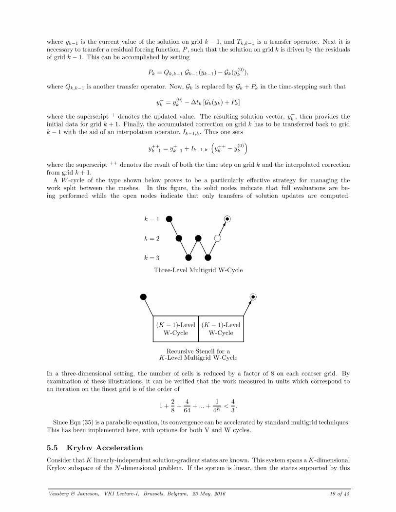
A W -cycle of the type shown below proves to be a particularly effective strategy for managing thework split between the meshes. In this figure, the solid nodes indicate that full evaluations are be-ing performed while the open nodes indicate that only transfers of solution updates are computed.

Three-Level Multigrid W-Cycle

k = 1

k = 2

k = 3

y

y

y

y

y

i

itAAAAAA

A

AA

Recursive Stencil for aK-Level Multigrid W-Cycle

(K − 1)-LevelW-Cycle

(K − 1)-LevelW-Cycle

y itAAA

In a three-dimensional setting, the number of cells is reduced by a factor of 8 on each coarser grid. Byexamination of these illustrations, it can be verified that the work measured in units which correspond toan iteration on the finest grid is of the order of

1 +2

8+

4

64+ ... +

1

4K<

4

3.

Since Eqn (35) is a parabolic equation, its convergence can be accelerated by standard multigrid techniques.This has been implemented here, with options for both V and W cycles.

5.5 Krylov Acceleration

Consider that K linearly-independent solution-gradient states are known. This system spans a K-dimensionalKrylov subspace of the N -dimensional problem. If the system is linear, then the states supported by this


subspace can be described by the following recombination of known y-G pairs.

y⋆ =

K∑

k=1

γkyk , G⋆ =

K∑

k=1

γk Gk,

whereK∑

k=1

γk = 1.

Convergence of the descent optimization procedures can be accelerated by minimizing the L2 Norm ofG⋆ to determine the appropriate recombination coefficients γk. See references [18, 19]. Now, the iterativeprocess becomes

yn+1j = y⋆

j − λG⋆j .

It should be noted that the above acceleration can fail if the preconditioned state of the current iterationis not linearly independent of the previous Krylov subspace. This can occur if the previous Krylov subspacehappens to contain the zero-gradient state, and this “failure” is fortuitous since the converged solution isprematurely determined. Another cause for failure is a poor choice of preconditioner, however, this shouldnot be the case with the method of steepest descent as the gradient at y⋆ should be nearly perpendicularto the previous Krylov subspace. In a linear setting, it is guaranteed that the new state as given by thepreconditioner is not contained within the previous Krylov subspace if the L2 Norm of the gradient of thenew state is less than that of G⋆ of the previous iteration.

5.6 Quasi-Newton Methods

Quasi-Newton methods are widely regarded as the method of choice for general optimization problemswhenever the gradient can be readily calculated. These methods estimate the Hessian (A) or its inverse(A−1) from changes in the gradient (δG) during the search steps. By the definition of A, to first order

δG = A δy.

Let Hn be an estimate of A−1 at the nth step. Then it should be required to satisfy

HnδGn = δyn. (41)

This can be satisfied by various recursive updating formulas for H , which also have the hereditary propertythat if A is constant, as is the case of a quadratic form, Eqn (41) holds for all of the previous steps δyk, k < n.Consequently H becomes an exact estimate of A−1 in N steps.

Three quasi-Newton methods have been tested in this work. The first is the rank one (R1) correction

Hn+1 = Hn +Pn(Pn)T

(Pn)T δGn. (42)

wherePn = δyn − HnδGn.

The second method is the Davidon-Fletcher-Powell (DFP) rank-two updating formula

Hn+1 = Hn

+δyn(δyn)T

(δyn)T δGn− HnδGn(δGn)T Hn

(δGn)T HnδGn. (43)

In order to assure N -step convergence for a quadratic form, this method requires the use of exact linesearches to find the minimum objective function in the search direction at each step. This is because thehereditary property depends on the orthogonality of each new gradient with the previous search direction,i.e., (Gn+1)T δyn = 0. Hence, many more evaluations of the objective function are required for DFP thanR1. However, DFP has an advantage in that the updated estimates of the inverse Hessian, Hn, remainpositive-definite.


The third quasi-Newton method tested uses the Broyden-Fanno-Goldfarb-Shannon (BFGS) updating for-mula

Hn+1 = Hn

+

(

1 +(δGn)T HnδGn

(δGn)T δyn

)

δyn(δyn)T

(δGn)T δyn

−HnδGn(δyn)T + δyn(δGn)T Hn

(δGn)T δyn. (44)

This corresponds to the DFP formula applied to estimate A rather than A−1. As with DFP, BFGS alsorequires exact line searches to assure N -step convergence for a quadratic form. In practice however, BFGSis usually preferred over DFP because it is considered to be more tolerant to inexact line searches, andtherefore a more robust procedure.

We should note that the line searches performed for the Rank-2 quasi-Newton methods were implementedto locate the position where the local gradient is orthogonal to the search direction. For the discretegradient, this location coincides with the minimum measurable cost function along the line. However, forthe continuous gradient, this may not be the case. The motivation for this choice of line search (as opposedto finding the minimum measurable cost) is to ensure that the Rank-2 systems remain positive-definite forthe continuous gradient optimizations. (See Reference [20], pp 54-55).

6 Results

The various methods described in this paper have been exercised to better understand their accuracy andperformance. Specifically, three items are addressed. The first is whether the discrete or the continuousgradient is necessarily better than the other either by yielding more accurate solutions, or by reducing thecost of the search procedure. The second is whether an alternate search strategy can be devised which outperforms the quasi-Newton approaches, when applied to trajectory and shape optimization problems, wherethe solution is expected to be smooth. And the third item discussed is regarding the robustness of the variousmethods as applied to the brachistochrone problem.

6.1 Accuracy

Both the continuous and discrete gradient-based optimizations have been applied to the brachistochroneproblem over a wide range of mesh sizes. The model problem analyzed in this work is given by Eqns (31& 32)with C = 1. Furthermore, to minimize the effects of the left-hand singularity, the boundary conditions weredetermined by using t0 = π

2 and t1 = π. A summary of this data related to accuracy is provided inFigures 17-21.

Figures 17&18 illustrate the convergence of the optimization process being driven by the continuous anddiscrete gradients, respectively. Here, the number of design variables is N = 31 and convergence is achievedusing the implicit stepping approach. Figure 19 is analogous to Figure 17 for the case of N = 511 designvariables. In these plots, the L2 Norm of both gradients and a measure of the converged path’s accuracy areprovided. The accuracy of these results are monitored with the root-mean-square difference of the optimizeddiscrete trajectory with that of the exact solution.

YERR =

√

∑N

j=1 (yj − yexact(xj))2

N

Whether the optimization is driven by the continuous or discrete gradient, the convergence histories lookvery similar. The main difference between these results is that the converged value of YERR levels off ata lower value for the continuous gradient (10−4.619) than it does for the discrete gradient (10−4.332). Thischaracter persists over the complete range of mesh sizes tested in this work as shown in Figure 20. Here,NX is the number of mesh intervals, thus N = NX − 1. While the advantage of the continuous gradientis apparent for the brachistochrone problem, in general, this may not be the case. Yet, these data clearlyillustrate that an optimization based on the discrete gradient is not necessarily the best choice. In eithercase, Figure 20 illustrates that both approaches are second-order accurate.


Using YERR as a measure of accuracy is only possible because the exact optimal solution is known for thisproblem. Typically, problems of optimization do not know what the exact solution is and therefore must relyon another figure of merit, usually the measurable cost function. For the brachistochrone problem, this isIR. Even though Figure 20 clearly illustrates that the continuous gradient is more accurate than the discretegradient, we know that IC

R will be greater than (or equal to) IDR by definition. Here IC

R is the measured costfunction as optimized by the continuous gradient, while ID

R is that optimized by the discrete gradient. Thissurplus, defined by

Surplus = ICR − ID

R

is illustrated in Figure 21 as a function of mesh size. Interpretating this surplus as a disadvantage of the con-tinuous gradient relative to the discrete gradient is unwarranted, as evidenced by Figure 20. However, sinceboth approaches are second-order accurate, it should come as no surprise that this surplus also diminishesin a second-order manner with increasing number of design variables.

6.2 Performance

The performances of the various optimization techniques are verified in this section. Detailed illustrationsof path histories as well as gradient convergences are given in Figures 22-38 for the different strategies on aproblem involving N = 31 & 511 design variables.

Since an implicit stepping for the brachistochrone is possible, its performance is used as a goal to achievein the design of an explicit scheme. As shown in Figures 22 & 24, the transient path shapes of the implicitscheme rapidly converges to the final state within a few iterations, regardless of problem dimension. Therapid convergence of this scheme is also exemplified by the quick decay of the corresponding gradients asshown in Figures 23 & 25.

Figures 26-29 provide path histories and gradient convergences for the three quasi-Newton methods. It isinteresting to note that the character of the paths from iteration to iteration is distinctly different than thatof the implicit scheme shown before in Figures 22 & 24. The main cause for this difference is that the quasi-Newton methods effectively take a uniform time step, whereas the other descent schemes investigated in thiswork employ a non-uniform time step dictated only by stability considerations. It is also interesting to notethat for N = 31, the two methods which estimate A−1 (Rank-1 and DFP), follow nearly identical convergencehistories, while the BFGS method requires about two extra iterations to converge the gradient norm to anequivalent level. For example, notice in Figure 27 that the Rank-1 and DFP schemes required 38 iterationsto converge the gradient 6 orders of magnitude, while BFGS took about 40 cycles. These quasi-Newtonmethods were tested on problems up to N = 511 design variables; they consistently exhibited a convergencebehavior where the gradient norm remains relatively flat until N iterations have been performed, then rapidlyconverging to machine-level zero in about 10 more steps. This behavior is precisely what the theory suggestsshould occur and this trend is definitely supported by Figures 27 & 29 for N = 31 & 511, respectively.However, the reader is reminded that the Rank-1 algorithm does not require a line search each iteration,and therefore may evaluate the gradient up to an order of magnitude fewer times than either of the Rank-2 schemes. Robustness issues aside, this can result in a significant difference in the computational timesbetween the various quasi-Newton methods.

Figures 30-31 give the results of the steepest descent approach. Recall that in Section 5.1 the stabilityanalysis of this stepping concluded that the number of iterations required for convergence was directlyproportional to N2. Even for the small case of N = 31 shown in these figures, more than 512 cycles wereperformed before the path visually converged and almost 6000 iterations were needed before machine-levelzero was attained. (Because of the CPU requirements involved, a solution for N = 511 was not evenattempted.) Clearly, this approach is unacceptable in the setting of large engineering problems of interest.In this solution, STEP = 1.0 was used as it provides the fastest convergence rates for the steepest descentapproach. A test with STEP = 1.01 verified our stability analysis as the solution quickly diverged.

In contrast with the previous results, the path history for a smoothed descent is illustrated in Figure 32.In this solution, STEP = 100 was used and to the eye, the final path is determined in less than 8 cycles.Figure 33 gives the convergence histories for a variety of values of STEP = 12.5, 25, 50, 100. These dataconfirm that a doubling of the step size essentially halves the number of iterations required for convergence,up to a point.

Figures 34-35 provide the results of applying the smoothed descent scheme coupled with Krylov acceler-ation. In this case, the path history looks to settle down after only 4 iterations while the gradient norm


exhibits a quadratic-like convergence behavior. Figure 35 indicates that the Krylov accelerated convergenceis almost invariant of the value of STEP in the preconditioned step. To obtain 6 orders of magnitudereduction requires between 12 & 14 steps for STEP ≥ 25. For reference, this figure also includes the bestconvergence curve of Figure 33 to better illustrate the positive effect that this acceleration scheme has onthe convergence of the optimization process.

Application of a multigrid W-cycle to drive the convergence of the brachistochrone is now studied. Fig-ures 36-37 give the corresponding path history and gradient convergence plots as seen before. Amazingly,the path of the second cycle is almost within symbol width of the final path. The effect of number of meshlevels, NMESH , used in the multigrid convergence is shown in Figure 37. Here, with NMESH = 1, asmoothed descent scheme is recovered; increasing the number of multigrid levels significantly increases theconvergence rate. Furthermore, while this figure depicts the convergence for NX = 32, it was observed thatthe multigrid convergence history was grid independent if one always used NMESH = log2(NX).

The enhancements incorporated beyond the original steepest descent method have systematically improvedthe convergence of the optimization process to the point where the performance of the implicit scheme hasbeen achieved. The final enhancement to the multigrid scheme is to incorporate the Krylov acceleration.Figure 38 compares the complete ensemble of enhancements to our explicit scheme with the performance ofthe implicit stepping. For all practical purposes, the convergence rates of these two schemes are identical.For comparison, this figure also includes the NMESH = 5 multigrid convergence of Figure 37, which isnoticeably slower than that with the Krylov acceleration. However, the convergence histories depicted inthis figure, for these three schemes, are essentially independent of the dimensionality, N . (See Figure 39.)

Figure 39 compares the performance of several of the various schemes. Here, ITERS is the number ofiterations required for the gradient norm to be reduced at least six orders of magnitude. This figure representsproblems ranging in size from N = 3 design variables up to N = 8191. (In this figure, NX is the numberof mesh intervals, thus N = NX − 1.) The basic steepest descent approach exhibits an O(N2) behavior inthe number of iterations required, while the quasi-Newton methods indicate O(N) as expected. Using thefull number of multigrid levels and Krylov acceleration provides a grid independent result, requiring about8 iterations to converge 6 orders. Finally, this is shown to compare favorably with the implicit steppingperformance which also yields a grid independent character, requiring only 7 iterations.

6.3 Robustness

We include a brief, qualitative synopsis of the robustness of the various schemes studied herein. While noattempt was made to establish a metric which one could monitor a scheme’s level of robustness, the successfulapplication of some of these methods proved to be sensitive to certain implementation issues. For example,and previously noted, the Krylov acceleration can “bomb” if a machine-level exact solution is found in lessthan N iterations. Figure 39 clearly shows that this occurred for all cases where N > 8.

The behavior of the robustness of the various quasi-Newton schemes seemed contrary to popular under-standing. The Rank-1 scheme had no issue converging any of the cases tested. This included optimizationsdriven by both the continuous and discrete gradients for problems with 3 ≤ N ≤ 511 design variables. How-ever, the Rank-2 schemes were fairly sensitive to the level of convergence of the line searches, and surprisingly,BFGS seemed more sensitive to “inexact” line searches than DFP.

Subject only to the stability limits discussed in § 5.1 & 5.2, the explicit time-stepping schemes of steepestdescent, smoothed steepest descent, and multigrid descent proved to be very robust. These optimizationsconverged as anticipated for every case tested. This included optimizations based on both the continuousand discrete gradients for problems up to N = 8191 design variables.

7 Conclusions

In this lecture, two model problems of optimization have been discussed. The first model problem of thespider-and-fly was used to introduce some basic concepts of optimization set up; it also illustrated somemental traps to avoid. The second model problem of the brachistochrone was used to develop variousaspects of the optimization process in much greater detail.

In the spider-fly problem, we showed how one can set up the objective function and its associated designspace, including constraints. Here, the cost function of the discrete problem was equivalent to that of thecontinuum; this is normally not the case. Direct differentiation of the cost function was used to establish the


gradient and Hessian matrix; also equivalent to that of the continuum. Steepest descent, Newton iteration,quasi-Newton, and Nash equilibrium methods were demonstrated. One trap avoided was on the choiceof which of these methods is most appropriate for optimizations that utilize design spaces of very largedimension. Another trap discussed was how a developer envisions the set up of the discrete problem.

A variety of optimization techniques have been applied to the brachistochrone problem. These includegradient approaches based on both the continuous as well as discrete forms. Results show that, at least forthe brachistochrone problem, the continuous gradient yields a slightly more accurate solution than does thediscrete gradient; a possible reason for this outcome is included.

The solution of the nonlinear optimization problem is accomplished with explicit and implicit time steppingschemes which are also compared with several quasi-Newton algorithms. The data presented herein illustratethat an explicit time-stepping scheme can be constructed whose convergence properties are invariant withthe dimensionality of the problem. Furthermore, the performance of this explicit scheme rivals that of theimplicit time stepping. These trends have been verified on problems ranging from N = 3 design variablesup to N = 8191 unknowns.

Finally, the performance of quasi-Newton methods is consistent with theoretical estimates in that theirconvergence (i.e., iterations required) is linearly dependent on the number of design variables.

For large engineering optimization problems of interest, N > O(103), it is obvious that quasi-Newtonmethods can become prohibitively expensive in terms of both computational and memory requirements.However, it is encouraging that the possibility exists of constructing an efficient explicit scheme based onthe straightforward techniques investigated under this research.

References

[1] H. E. Dudeney. The Spider and The Fly. The Weekly Dispatch Newspaper, 14 June 1903. Also publishedin The Canterbury Puzzles and Other Curious Problems, London, 1907.

[2] W. K. Anderson, III J. C. Newman, D. L. Whitfield, and E. J. Nielsen. Sensitivity analysis for Navier-Stokes equations on unstructured meshes using complex variables. AIAA Journal, 39(1):56–63, January2001. Also, AIAA Paper 99-3294.

[3] S. Boyd and L. Vandenberghe. Convex Optimization. Cambridge University Press, New York, NY,2004. ISBN 0 521 83378 7.

[4] Johann Bernoulli. Acta Eruditorum. J.F. Gleditsch Publishing, Leipzig, Germany, June 1696. OttoMencke, Editor.

[5] Galileo Galilei. Discourses and mathematical demonstrations concerning the two new sciences. Pub-lished, Leyden, Holland, 1638.

[6] A. Jameson and J. C. Vassberg. Studies of alternative numerical optimization methods applied to thebrachistochrone problem. Computational Fluid Dynamics Journal, 9(3), October 2000. Special Issueon CFD and Education, Dedicated to Dr. Koichi Oshima; Emeritus Professor of University of Tokyo.

[7] A. Jameson and J. C. Vassberg. Studies of alternative numerical optimization methods applied to thebrachistochrone problem. In Proceedings of OptiCON’99, Newport Beach, CA, October 1999.

[8] G. B. Thomas. Calculus and Analytic Geometry. Addison-Wesley, Reading, MA, 1960. Series inMathematics.

[9] E. Chong and S. Zak. Introduction to Optimization. Wiley, New York, NY, 1995.

[10] R. P. Fedorenko. The speed of convergence of one iterative process. Comp. Mathematics and Mathe-

matical Physics, 4:227–235, 1964.

[11] A. Brandt. Multi-level adaptive solutions to boundary value problems. Mathematical Computing,31:333–390, 1977.

[12] W. Hackbusch. On the multi-grid method applied to difference equations. Computing, 20:291–306,1978.


[13] R. H. Ni. A multiple grid scheme for solving the Euler equations. AIAA Journal, 20:1565–1571, 1982.

[14] M. G. Hall. Cell vertex multigrid schemes for solution of the Euler equations. Reading, April 1985.Proceedings IMA Conference on Numerical Methods for Fluid Dynamics.

[15] A. Jameson. Multigrid algorithms for compressible flow calculations. In W. Hackbusch and U. Trotten-berg, editors, Lecture Notes in Mathematics, Vol. 1228, pages 166–201. 2nd European Conf. MultigridMethods, Cologne, 1985, Springer-Verlag, 1986.

[16] A. Jameson. Solution of the Euler equations for two dimensional transonic flow by a multigrid method.Applied Mathematics and Computations, 13:327–356, 1983.

[17] A. Jameson. Solution of the Euler equations by a multigrid method. Applied Mathematics and Com-

putations, 13:327–356, 1983.

[18] Y. Saad. Iterative Methods for Sparse Linear Systems. PWS Publishing Company, Boston, MA, 1996.PWS Series in Computer Science.

[19] R. W. Clark. A new iterative matrix solution procedure for three-dimension panel methods. AIAA

paper 85-0176, AIAA Aerospace Sciences Meeting, Reno, NV, January 1985.

[20] R. Fletcher. Practical Methods of Optimization. John Wiley & Sons, New York, NY, 1995. SecondEdition.


Block Size

4" x 4" x 12"

Path Length 16.00"

SPIDER FLY PATH

Figure 1: Obvious local-minimum path between Spider and Fly.

Block Size

4" x 4" x 12"

Path Length Sqrt(250.0)"

~ 15.81"

SPIDER FLY PATH

Figure 2: Non-obvious global-minimum path between Spider and Fly.


00

-1

-2

-3

-4

-5

-6

-7

-8

-9

0 50 100 150 200 250 3000

Iteration

LO

G_1

0 (

GR

MS

)

Step: 1.885

Figure 3: Convergence of Gradient for Steepest Descent.

1.9

2.0

2.1

2.2

2.3

2.4

2.5

2.6

2.7

4.9

5.0

5.1

5.2

5.3

5.4

5.5

5.6

5.7

5.8

5.9

6.0

6.1

Baseline

Optimum

Top View

Y

X

1.6

1.7

1.8

1.9

2.0

2.1

4.9

5.0

5.1

5.2

5.3

5.4

5.5

5.6

5.7

5.8

5.9

6.0

6.1

Baseline

Optimum

Side View

Y

Z

Figure 4: Steepest-Descent Trajectory through the Design Space.


00

-1

-2

-3

-4

-5

-6

-7

-8

-9

0 1 2 3 40

Iteration

LO

G_1

0 (

GR

MS

)

Figure 5: Convergence of Gradient for Newton Iteration.

1.9

2.0

2.1

2.2

2.3

2.4

2.5

2.6

2.7

4.9

5.0

5.1

5.2

5.3

5.4

5.5

5.6

5.7

5.8

5.9

6.0

6.1

Baseline

Optimum

Top View

Y

X

1.6

1.7

1.8

1.9

2.0

2.1

4.9

5.0

5.1

5.2

5.3

5.4

5.5

5.6

5.7

5.8

5.9

6.0

6.1

Baseline

Optimum

Side View

Y

Z

Figure 6: Newton-Iteration Trajectory through the Design Space.


00

-1

-2

-3

-4

-5

-6

-7

-8

-9

0 1 2 3 4 5 6 7 8 9 100

Iteration

LO

G_1

0 (

GR

MS

)

Figure 7: Convergence of Gradient for Rank-1 quasi-Newton Iteration.

1.9

2.0

2.1

2.2

2.3

2.4

2.5

2.6

2.7

4.9

5.0

5.1

5.2

5.3

5.4

5.5

5.6

5.7

5.8

5.9

6.0

6.1

Baseline

Optimum

Top View

Y

X

1.6

1.7

1.8

1.9

2.0

2.1

4.9

5.0

5.1

5.2

5.3

5.4

5.5

5.6

5.7

5.8

5.9

6.0

6.1

Baseline

Optimum

Side View

Y

Z

Figure 8: Rank-1 quasi-Newton Trajectory through the Design Space.


00

-2

-4

-6

-8

-10

-12

-14

0 2 4 6 8 10 12 14 16 18 200

Iteration

LO

G_1

0 (

ER

RO

R )

Nash Cycle

X Sub-Iter

Y Sub-Iter

Z Sub-Iter

00

-1

-2

-3

-4

-5

-6

-7

-8

-9

0 2 4 6 8 10 12 14 16 18 200

Iteration

LO

G_1

0 (

GR

MS

)

Nash Cycle

X Sub-Iter

Y Sub-Iter

Z Sub-Iter

Figure 9: Convergence of Error and Gradient for Nash Equilibrium.

1.9

2.0

2.1

2.2

2.3

2.4

2.5

2.6

2.7

4.9

5.0

5.1

5.2

5.3

5.4

5.5

5.6

5.7

5.8

5.9

6.0

6.1

Baseline

Optimum

Top View

Y

X

1.6

1.7

1.8

1.9

2.0

2.1

4.9

5.0

5.1

5.2

5.3

5.4

5.5

5.6

5.7

5.8

5.9

6.0

6.1

Baseline

Optimum

Side View

Y

Z

Figure 10: Nash Equilibrium Trajectory through the Design Space.


Block Size

4" x 4" x 12"

Path Length 16.00"

SPIDER FLY PATH

Figure 11: Obvious local-minimum path between Spider and Fly on flattened box.

Block Size

4" x 4" x 12"

Path Length Sqrt(250.0)"

~ 15.81"

SPIDER FLY PATH

Figure 12: Non-obvious global-minimum path between Spider and Fly on flattened box.


00

-1

-2

-3

-4

-5

-6

-7

-8

0 10 20 30 40 50 600

Iteration

LO

G_1

0 (

GR

MS

)

Step: 1.885

Figure 13: Convergence of Gradient for Steepest Descent with S2 ≤ 4.

1.9

2.0

2.1

2.2

2.3

2.4

2.5

2.6

2.7

2.8

3.0

3.5

4.0

4.5

5.0

5.5

6.0

6.5

Baseline

Optimum

Top View

Y

X

1.5

1.6

1.7

1.8

1.9

2.0

2.1

3.0

3.5

4.0

4.5

5.0

5.5

6.0

6.5

Baseline

Optimum

Side View

Y

Z

Figure 14: Steepest-Descent Trajectory through the Design Space with S2 ≤ 4.


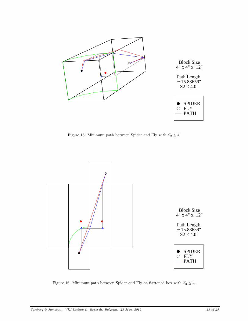
Block Size

4" x 4" x 12"

Path Length ~ 15.83659"

S2 < 4.0"

SPIDER FLY PATH

Figure 15: Minimum path between Spider and Fly with S2 ≤ 4.

Block Size

4" x 4" x 12"

Path Length ~ 15.83659"

S2 < 4.0"

SPIDER FLY PATH

Figure 16: Minimum path between Spider and Fly on flattened box with S2 ≤ 4.


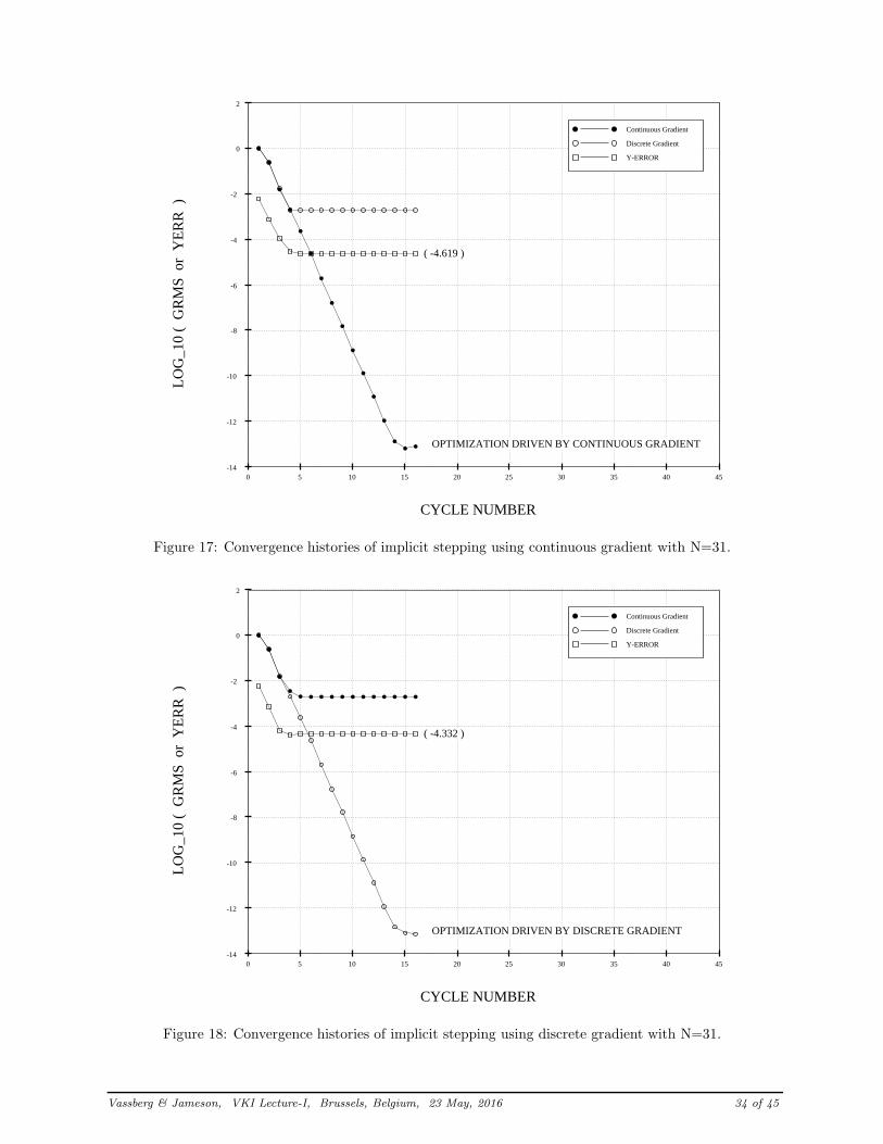
0 5 10 15 20 25 30 35 40 45-14

-12

-10

-8

-6

-4

-2

0

2

OPTIMIZATION DRIVEN BY CONTINUOUS GRADIENT

( -4.619 )

CYCLE NUMBER

LO

G_1

0 (

GR

MS

or

YE

RR

)

Continuous Gradient

Discrete Gradient

Y-ERROR

Figure 17: Convergence histories of implicit stepping using continuous gradient with N=31.

0 5 10 15 20 25 30 35 40 45-14

-12

-10

-8

-6

-4

-2

0

2

OPTIMIZATION DRIVEN BY DISCRETE GRADIENT

( -4.332 )

CYCLE NUMBER

LO

G_1

0 (

GR

MS

or

YE

RR

)

Continuous Gradient

Discrete Gradient

Y-ERROR

Figure 18: Convergence histories of implicit stepping using discrete gradient with N=31.


0 5 10 15 20 25 30 35 40 45-14

-12

-10

-8

-6

-4

-2

0

2N = 511

OPTIMIZATION DRIVEN BY CONTINUOUS GRADIENT

( -7.020 )

CYCLE NUMBER

LO

G_1

0 (

GR

MS

or

YE

RR

)

Continuous Gradient

Discrete Gradient

Y-ERROR

Figure 19: Convergence histories of implicit stepping using continuous gradient with N=511.


3 4 5 6 7 8 9 10 11 12 13-10

-9

-8

-7

-6

-5

-4

-3

N =

31

N =

511

N =

127

N =

204

7

Log_2 ( NX )

Log

_10

( Y

ER

R )

CONT

DISC

1st-order

2nd-order

3rd-order

Figure 20: Computed path errors as a function of mesh size.

3 4 5 6 7 8 9-13

-12

-11

-10

-9

-8

-7

-6

-5

-4

N =

31

N =

511

Log_2 ( NX )

Log

_10

( S

urpl

us )

Figure 21: Difference of measurable cost function between the continuous and discrete gradients.


0.1 0.2 0.3 0.4 0.5 0.6 0.7 0.8 0.9 1.0-0.65

-0.60

-0.55

-0.50

-0.45

-0.40

-0.35

-0.30

X

Y

Exact

cyc 1

cyc 2

cyc 4

Figure 22: History of paths of implicit stepping with N=31.

0 5 10 15 20 25 30 35 40 45-14

-12

-10

-8

-6

-4

-2

0

2

CYCLE NUMBER

LO

G_1

0 (

GR

MS

)

Figure 23: Convergence history of implicit stepping with N=31.


0.1 0.2 0.3 0.4 0.5 0.6 0.7 0.8 0.9 1.0-0.65

-0.60

-0.55

-0.50

-0.45

-0.40

-0.35

-0.30

X

Y

Exact

cyc 1

cyc 2

cyc 4

Figure 24: History of paths of implicit stepping with N=511.

0 5 10 15 20 25 30 35 40 45-12

-10

-8

-6

-4

-2

0

2

CYCLE NUMBER

LO

G_1

0 (

GR

MS

)

Figure 25: Convergence history of implicit stepping with N=511.


0.1 0.2 0.3 0.4 0.5 0.6 0.7 0.8 0.9 1.0-0.65

-0.60

-0.55

-0.50

-0.45

-0.40

-0.35

-0.30

X

Y

Exact

cyc 1

cyc 5

cyc 9

cyc 13

cyc 17

cyc 21

cyc 25

cyc 29

cyc 33

cyc 37

Figure 26: History of paths for Rank-1 quasi-Newton with N=31.

0 5 10 15 20 25 30 35 40 45-12

-10

-8

-6

-4

-2

0

2

CYCLE NUMBER

LO

G_1

0 (

GR

MS

)

Rank One

DFP

BFGS

Figure 27: Comparison of quasi-Newton convergence histories with N=31.


0.1 0.2 0.3 0.4 0.5 0.6 0.7 0.8 0.9 1.0-0.65

-0.60

-0.55

-0.50

-0.45

-0.40

-0.35

-0.30

X

Y

Exact

cyc 1

cyc 65

cyc 129

cyc 193

cyc 257

cyc 321

cyc 385

cyc 449

cyc 513

cyc 577

Figure 28: History of paths for Rank-1 quasi-Newton with N=511.

0 100 200 300 400 500 600-12

-10

-8

-6

-4

-2

0

2

CYCLE NUMBER

LO

G_1

0 (

GR

MS

)

Rank One

DFP

BFGS

Figure 29: Comparison of quasi-Newton convergence histories with N=511.


0.1 0.2 0.3 0.4 0.5 0.6 0.7 0.8 0.9 1.0-0.65

-0.60

-0.55

-0.50

-0.45

-0.40

-0.35

-0.30

X

Y

Exact

cyc 1

cyc 2

cyc 4

cyc 8

cyc 16

cyc 32

cyc 64

cyc 128

cyc 256

cyc 512

cyc 1024

cyc 2048

cyc 4096

cyc 8192

Figure 30: History of paths of steepest descent with N=31.

0 1000 2000 3000 4000 5000 6000 7000 8000 9000-14

-12

-10

-8

-6

-4

-2

0

2

CYCLE NUMBER

LO

G_1

0 (

GR

MS

)

Figure 31: Convergence history of steepest descent with N=31.


0.1 0.2 0.3 0.4 0.5 0.6 0.7 0.8 0.9 1.0-0.65

-0.60

-0.55

-0.50

-0.45

-0.40

-0.35

-0.30

X

Y

Exact

cyc 1

cyc 2

cyc 4

cyc 8

cyc 32

cyc 64

Figure 32: History of paths of smoothed descent with N=31 & STEP=100.

0 50 100 150 200 250 300 350 400 450 500-14

-12

-10

-8

-6

-4

-2

0

2

CYCLE NUMBER

LO

G_1

0 (

GR

MS

)

STEP = 100

STEP = 50

STEP = 25

STEP = 12.5

Figure 33: Convergence history of smoothed descent with N=31.


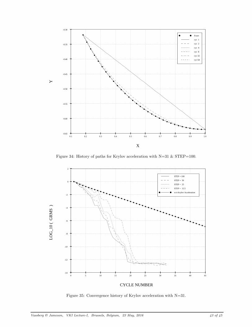
0.1 0.2 0.3 0.4 0.5 0.6 0.7 0.8 0.9 1.0-0.65

-0.60

-0.55

-0.50

-0.45

-0.40

-0.35

-0.30

X

Y

Exact

cyc 1

cyc 2

cyc 4

cyc 8

cyc 32

cyc 64

Figure 34: History of paths for Krylov acceleration with N=31 & STEP=100.

0 5 10 15 20 25 30 35 40 45-14

-12

-10

-8

-6

-4

-2

0

2

CYCLE NUMBER

LO

G_1

0 (

GR

MS

)

STEP = 100

STEP = 50

STEP = 25

STEP = 12.5

w/o Krylov Acceleration

Figure 35: Convergence history of Krylov acceleration with N=31.


0.1 0.2 0.3 0.4 0.5 0.6 0.7 0.8 0.9 1.0-0.65

-0.60

-0.55

-0.50

-0.45

-0.40

-0.35

-0.30

STEP = 2.0 , SMOO = 0.75

NMESH = 5

X

Y

Exact

cyc 1

cyc 2

cyc 4

cyc 8

cyc 32

cyc 64

Figure 36: History of paths for multigrid acceleration with N=31.

0 5 10 15 20 25 30 35 40 45-14

-12

-10

-8

-6

-4

-2

0

2

STEP = 2.0 , SMOO = 0.75

CYCLE NUMBER

LO

G_1

0 (

GR

MS

)

NMESH = 5

NMESH = 4

NMESH = 3

NMESH = 2

NMESH = 1

Figure 37: Convergence history of multigrid acceleration with N=31.


0 5 10 15 20 25 30 35 40 45-14

-12

-10

-8

-6

-4

-2

0

2

CYCLE NUMBER

LO

G_1

0 (

GR

MS

)

MG w/ Krylov Acceleration

MG w/o Krylov Acceleration

Implicit Stepping

Figure 38: Comparison of grid-independent convergence histories.

1 2 3 4 5 6 7 8 9 10 11 12 13 140

2

4

6

8

10

12

14

16

N =

31

N =

511

N =

819

1

Log_2 ( NX )

Log

_2 (

IT

ER

S )

Steepest Descent

Rank-1 Quasi-Newton

Multigrid W-Cycle

Multigrid w/ Krylov Acceleration

Implicit Stepping

Figure 39: Comparison of convergence properties with dependence on dimensionality.


introduction to optimization and multidisciplinary...

Documents