introduction to numerical analysis - math.iitb.ac.insiva/si50716/si507lecturenotes.pdf ·...
TRANSCRIPT
Introduction toNumerical Analysis
Lecture Notes for SI 507
Authors:
S. Baskar and S. Sivaji Ganesh
Department of MathematicsIndian Institute of Technology Bombay
Powai, Mumbai 400 076.

Contents
1 Mathematical Preliminaries . . . . . . . . . . . . . . . . . . . . . . . . . . . . . . . . . . . . . 7
1.1 Sequences of Real Numbers . . . . . . . . . . . . . . . . . . . . . . . . . . . . . . . . . . . . . 7
1.2 Limits and Continuity . . . . . . . . . . . . . . . . . . . . . . . . . . . . . . . . . . . . . . . . . . 9
1.3 Differentiation . . . . . . . . . . . . . . . . . . . . . . . . . . . . . . . . . . . . . . . . . . . . . . . . . 12
1.4 Integration . . . . . . . . . . . . . . . . . . . . . . . . . . . . . . . . . . . . . . . . . . . . . . . . . . . . 15
1.5 Taylor’s Theorem . . . . . . . . . . . . . . . . . . . . . . . . . . . . . . . . . . . . . . . . . . . . . . 16
1.6 Orders of Convergence . . . . . . . . . . . . . . . . . . . . . . . . . . . . . . . . . . . . . . . . . . 20
1.6.1 Big Oh and Little oh Notations . . . . . . . . . . . . . . . . . . . . . . . . . . . . . 21
1.6.2 Rates of Convergence . . . . . . . . . . . . . . . . . . . . . . . . . . . . . . . . . . . . . . 23
1.7 Exercises . . . . . . . . . . . . . . . . . . . . . . . . . . . . . . . . . . . . . . . . . . . . . . . . . . . . . 24
2 Error Analysis . . . . . . . . . . . . . . . . . . . . . . . . . . . . . . . . . . . . . . . . . . . . . . . . . . . 29
2.1 Floating-Point Representation . . . . . . . . . . . . . . . . . . . . . . . . . . . . . . . . . . . 30
2.1.1 Floating-Point Approximation . . . . . . . . . . . . . . . . . . . . . . . . . . . . . . 30
2.1.2 Underflow and Overflow of Memory . . . . . . . . . . . . . . . . . . . . . . . . . 31
2.1.3 Chopping and Rounding a Number . . . . . . . . . . . . . . . . . . . . . . . . . . 33
2.1.4 Arithmetic Using n-Digit Rounding and Chopping . . . . . . . . . . . . 35
2.2 Types of Errors . . . . . . . . . . . . . . . . . . . . . . . . . . . . . . . . . . . . . . . . . . . . . . . . 36
2.3 Loss of Significance . . . . . . . . . . . . . . . . . . . . . . . . . . . . . . . . . . . . . . . . . . . . 37
2.4 Propagation of Relative Error in Arithmetic Operations . . . . . . . . . . . . . 40
2.4.1 Addition and Subtraction . . . . . . . . . . . . . . . . . . . . . . . . . . . . . . . . . . 40
2.4.2 Multiplication . . . . . . . . . . . . . . . . . . . . . . . . . . . . . . . . . . . . . . . . . . . . 41
2.4.3 Division . . . . . . . . . . . . . . . . . . . . . . . . . . . . . . . . . . . . . . . . . . . . . . . . . 42
2.4.4 Total Error . . . . . . . . . . . . . . . . . . . . . . . . . . . . . . . . . . . . . . . . . . . . . . 42
2.5 Propagation of Relative Error in Function Evaluation . . . . . . . . . . . . . . . 43
2.5.1 Stable and Unstable Computations . . . . . . . . . . . . . . . . . . . . . . . . . . 46
2.6 Exercises . . . . . . . . . . . . . . . . . . . . . . . . . . . . . . . . . . . . . . . . . . . . . . . . . . . . . 48
3 Numerical Linear Algebra . . . . . . . . . . . . . . . . . . . . . . . . . . . . . . . . . . . . . . . 51
3.1 System of Linear Equations . . . . . . . . . . . . . . . . . . . . . . . . . . . . . . . . . . . . . 52
3.2 Direct Methods for Linear Systems . . . . . . . . . . . . . . . . . . . . . . . . . . . . . . . 53
3.2.1 Naive Gaussian Elimination Method . . . . . . . . . . . . . . . . . . . . . . . . . 53
3.2.2 Modified Gaussian Elimination Method with Partial Pivoting . . . 57
3.2.3 Operations Count in Naive Gaussian Elimination Method . . . . . . 59
3.2.4 Thomas Method for Tri-diagonal System . . . . . . . . . . . . . . . . . . . . . 60
3.2.5 LU Factorization . . . . . . . . . . . . . . . . . . . . . . . . . . . . . . . . . . . . . . . . . 62
3.3 Matrix Norms and Condition Number of a Matrix . . . . . . . . . . . . . . . . . . 73
3.4 Iterative Methods for Linear Systems . . . . . . . . . . . . . . . . . . . . . . . . . . . . . 80
3.4.1 Jacobi Method . . . . . . . . . . . . . . . . . . . . . . . . . . . . . . . . . . . . . . . . . . . 81
3.4.2 Gauss-Seidel Method . . . . . . . . . . . . . . . . . . . . . . . . . . . . . . . . . . . . . . 85
3.4.3 Mathematical Error . . . . . . . . . . . . . . . . . . . . . . . . . . . . . . . . . . . . . . . 87
3.4.4 Residual Corrector Method . . . . . . . . . . . . . . . . . . . . . . . . . . . . . . . . 88
3.4.5 Stopping Criteria . . . . . . . . . . . . . . . . . . . . . . . . . . . . . . . . . . . . . . . . . 91
3.5 Eigenvalue Problems . . . . . . . . . . . . . . . . . . . . . . . . . . . . . . . . . . . . . . . . . . . 91
3.5.1 Power Method . . . . . . . . . . . . . . . . . . . . . . . . . . . . . . . . . . . . . . . . . . . . 92
3.5.2 Gerschgorin’s Theorem . . . . . . . . . . . . . . . . . . . . . . . . . . . . . . . . . . . . 107
3.6 Exercises . . . . . . . . . . . . . . . . . . . . . . . . . . . . . . . . . . . . . . . . . . . . . . . . . . . . . 110
4 Nonlinear Equations . . . . . . . . . . . . . . . . . . . . . . . . . . . . . . . . . . . . . . . . . . . . . 119
4.1 Closed Domain Methods . . . . . . . . . . . . . . . . . . . . . . . . . . . . . . . . . . . . . . . . 120
4.1.1 Bisection Method . . . . . . . . . . . . . . . . . . . . . . . . . . . . . . . . . . . . . . . . . 120
4.1.2 Regula-falsi Method . . . . . . . . . . . . . . . . . . . . . . . . . . . . . . . . . . . . . . . 125
4.2 Stopping Criteria . . . . . . . . . . . . . . . . . . . . . . . . . . . . . . . . . . . . . . . . . . . . . . 131
4.3 Open Domain Methods . . . . . . . . . . . . . . . . . . . . . . . . . . . . . . . . . . . . . . . . . 132
4.3.1 Secant Method . . . . . . . . . . . . . . . . . . . . . . . . . . . . . . . . . . . . . . . . . . . 133
4.3.2 Newton-Raphson Method . . . . . . . . . . . . . . . . . . . . . . . . . . . . . . . . . . 135
4.3.3 Fixed-Point Iteration Method . . . . . . . . . . . . . . . . . . . . . . . . . . . . . . 140
4.4 Comparison and Pitfalls of Iterative Methods . . . . . . . . . . . . . . . . . . . . . . 148
4.5 Exercises . . . . . . . . . . . . . . . . . . . . . . . . . . . . . . . . . . . . . . . . . . . . . . . . . . . . . 151
5 Interpolation . . . . . . . . . . . . . . . . . . . . . . . . . . . . . . . . . . . . . . . . . . . . . . . . . . . . 159
5.1 Polynomial Interpolation . . . . . . . . . . . . . . . . . . . . . . . . . . . . . . . . . . . . . . . . 160
5.1.1 Existence and Uniqueness of Interpolating Polynomial . . . . . . . . . 160
5.1.2 Lagrange’s Form of Interpolating Polynomial . . . . . . . . . . . . . . . . . 163
5.1.3 Newton’s Form of Interpolating Polynomial . . . . . . . . . . . . . . . . . . 166
5.2 Newton’s Divided Difference Formulas . . . . . . . . . . . . . . . . . . . . . . . . . . . . 167
5.2.1 Divided Differences Table . . . . . . . . . . . . . . . . . . . . . . . . . . . . . . . . . . 170
5.2.2 Divided Difference Formula for Repeated Nodes . . . . . . . . . . . . . . . 171
5.3 Error in Polynomial Interpolation . . . . . . . . . . . . . . . . . . . . . . . . . . . . . . . . 174
5.3.1 Mathematical Error . . . . . . . . . . . . . . . . . . . . . . . . . . . . . . . . . . . . . . . 175
5.3.2 Arithmetic Error . . . . . . . . . . . . . . . . . . . . . . . . . . . . . . . . . . . . . . . . . 177
5.3.3 Total Error . . . . . . . . . . . . . . . . . . . . . . . . . . . . . . . . . . . . . . . . . . . . . . 179
5.3.4 Runge Phenomenon . . . . . . . . . . . . . . . . . . . . . . . . . . . . . . . . . . . . . . . 180
5.3.5 Convergence of Sequence of Interpolating Polynomials . . . . . . . . . 181
5.4 Piecewise Polynomial Interpolation . . . . . . . . . . . . . . . . . . . . . . . . . . . . . . . 183
5.5 Spline Interpolation . . . . . . . . . . . . . . . . . . . . . . . . . . . . . . . . . . . . . . . . . . . . 185
5.6 Exercises . . . . . . . . . . . . . . . . . . . . . . . . . . . . . . . . . . . . . . . . . . . . . . . . . . . . . 188
6 Numerical Integration and Differentiation . . . . . . . . . . . . . . . . . . . . . . . 195
6.1 Numerical Integration . . . . . . . . . . . . . . . . . . . . . . . . . . . . . . . . . . . . . . . . . . 195
6.1.1 Rectangle Rule . . . . . . . . . . . . . . . . . . . . . . . . . . . . . . . . . . . . . . . . . . . 196
6.1.2 Trapezoidal Rule . . . . . . . . . . . . . . . . . . . . . . . . . . . . . . . . . . . . . . . . . 198
6.1.3 Simpson’s Rule . . . . . . . . . . . . . . . . . . . . . . . . . . . . . . . . . . . . . . . . . . . 201
6.1.4 Method of Undetermined Coefficients . . . . . . . . . . . . . . . . . . . . . . . . 204
6.1.5 Gaussian Rules . . . . . . . . . . . . . . . . . . . . . . . . . . . . . . . . . . . . . . . . . . . 206
6.2 Numerical Differentiation . . . . . . . . . . . . . . . . . . . . . . . . . . . . . . . . . . . . . . . 209
6.2.1 Approximations of First Derivative . . . . . . . . . . . . . . . . . . . . . . . . . . 209
6.2.2 Methods based on Interpolation . . . . . . . . . . . . . . . . . . . . . . . . . . . . 212
6.2.3 Methods based on Undetermined Coefficients . . . . . . . . . . . . . . . . . 215
6.2.4 Arithmetic Error in Numerical Differentiation . . . . . . . . . . . . . . . . 216
6.3 Exercises . . . . . . . . . . . . . . . . . . . . . . . . . . . . . . . . . . . . . . . . . . . . . . . . . . . . . 218
7 Numerical Ordinary Differential Equations . . . . . . . . . . . . . . . . . . . . . . 223
7.1 Review of Theory . . . . . . . . . . . . . . . . . . . . . . . . . . . . . . . . . . . . . . . . . . . . . . 224
7.2 Discretization Notations . . . . . . . . . . . . . . . . . . . . . . . . . . . . . . . . . . . . . . . . 227
7.3 Euler’s Method . . . . . . . . . . . . . . . . . . . . . . . . . . . . . . . . . . . . . . . . . . . . . . . . 228
7.3.1 Error in Euler’s Method . . . . . . . . . . . . . . . . . . . . . . . . . . . . . . . . . . . 230
7.4 Modified Euler’s Methods . . . . . . . . . . . . . . . . . . . . . . . . . . . . . . . . . . . . . . . 234
7.5 Runge-Kutta Methods . . . . . . . . . . . . . . . . . . . . . . . . . . . . . . . . . . . . . . . . . . 236
7.5.1 Order Two . . . . . . . . . . . . . . . . . . . . . . . . . . . . . . . . . . . . . . . . . . . . . . . 236
7.5.2 Order Four . . . . . . . . . . . . . . . . . . . . . . . . . . . . . . . . . . . . . . . . . . . . . . 238
7.6 Exercises . . . . . . . . . . . . . . . . . . . . . . . . . . . . . . . . . . . . . . . . . . . . . . . . . . . . . 238
Index . . . . . . . . . . . . . . . . . . . . . . . . . . . . . . . . . . . . . . . . . . . . . . . . . . . . . . . . . . . . . . . 241
Baskar and Sivaji6
S I 507, IITB
CHAPTER 1
Mathematical Preliminaries
This chapter reviews some of the concepts and results from calculus that are fre-quently used in this course. We recall important definitions and theorems whoseproof is outlined briefly. The readers are assumed to be familiar with a first coursein calculus.
In Section 1.1, we introduce sequences of real numbers and discuss the concept oflimit and continuity in Section 1.2 with the intermediate value theorem. This theoremplays a basic role in finding initial guesses in iterative methods for solving nonlinearequations. In Section 1.3 we define derivative of a function, and prove Rolle’s theoremand mean-value theorem for derivatives. The mean-value theorem for integration isdiscussed in Section 1.4. These two theorems are crucially used in devising methodsfor numerical integration and differentiation. Finally, Taylor’s theorem is discussed inSection 1.5, which is essential for derivation and error analysis of almost all numericalmethods discussed in this course. In Section 1.6 we introduce tools useful in discussingspeed of convergence of sequences and rate at which a function fpxq approaches apoint fpx0q as x Ñ x0.
Let a, b P R be such that a ă b. We use the notations ra, bs and pa, bq for the closedand the open intervals, respectively, and are defined by
ra, bs “ t x P R : a ď x ď b u and pa, bq “ t x P R : a ă x ă b u.
1.1 Sequences of Real Numbers
Definition 1.1 (Sequence).
A sequence of real numbers is an ordered list of real numbers
a1, a2, ¨ ¨ ¨ , an, an`1, ¨ ¨ ¨
In other words, a sequence is a function that associates the real number an foreach natural number n. The notation tanu is often used to denote the sequencea1, a2, ¨ ¨ ¨ , an, an`1, ¨ ¨ ¨
Chapter 1. Mathematical Preliminaries
The concept of convergence of a sequence plays an important role in numerical anal-ysis, for instance when approximating a solution x of a certain problem via an iter-ative procedure that produces a sequence of approximation. Here, we are interestedin knowing the convergence of the sequence of approximate solutions to the exactsolution x.
Definition 1.2 (Convergence of a Sequence).
Let tanu be a sequence of real numbers and let L be a real number. The sequencetanu is said to converge to L, and we write
limnÑ8
an “ L(or an Ñ L as n Ñ 8),
if for every ϵ ą 0 there exists a natural number N such that
|an ´ L| ă ϵ whenever n ě N.
The real number L is called the limit of the sequence tanu.
Theorem 1.3 (Sandwich Theorem).
Let tanu, tbnu, tcnu be sequences of real numbers such that
(1) there exists an n0 P N such that for every n ě n0, the sequences satisfy theinequalities an ď bn ď cn and
(2) limnÑ8
an “ limnÑ8
cn “ L.
Then the sequence tbnu also converges and limnÑ8
bn “ L. [\
Definition 1.4 (Bounded Sequence).
A sequence tanu is said to be a bounded sequence if there exists a real numberM such that
|an| ď M for every n P N.
Theorem 1.5 (Bolzano-Weierstrass theorem). Every bounded sequence tanu hasa convergent subsequence tank
u.
The following result is very useful in computing the limit of a sequence sandwichedbetween two sequences having a common limit.
Definition 1.6 (Monotonic Sequences).
A sequence tanu of real numbers is said to be
(1) an increasing sequence if an ď an`1, for every n P N.
Baskar and Sivaji8
S I 507, IITB
Section 1.2. Limits and Continuity
(2) a strictly increasing sequence if an ă an`1, for every n P N.
(3) a decreasing sequence if an ě an`1, for every n P N.
(4) a strictly decreasing sequence if an ą an`1, for every n P N.
A sequence tanu is said to be a (strictly) monotonic sequence if it is either(strictly) increasing or (strictly) decreasing.
Theorem 1.7. Bounded monotonic sequences always converge. [\
Note that any bounded sequence need not converge. The monotonicity in the abovetheorem is very important. The following result is known as “algebra of limits ofsequences”.
Theorem 1.8. Let tanu and tbnu be two sequences. Assume that limnÑ8
an and limnÑ8
bn
exist. Then
(1) limnÑ8
pan ` bnq “ limnÑ8
an ` limnÑ8
bn.
(2) limnÑ8
c an “ c limnÑ8
an, for any number c.
(3) limnÑ8
anbn “ limnÑ8
an limnÑ8
bn .
(4) limnÑ8
1
an“
1
limnÑ8
an, provided lim
nÑ8an ‰ 0.
1.2 Limits and Continuity
In the previous section, we introduced the concept of limit for a sequences of realnumbers. We now define the “limit” in the context of functions.
Definition 1.9 (Limit of a Function).
(1) Let f be a function defined on the left side (or both sides) of a, except possibly ata itself. Then, we say “the left-hand limit of fpxq as x approaches a, equals l”and denote
limxÑa´
fpxq “ l,
if we can make the values of fpxq arbitrarily close to l (as close to l as we like)by taking x to be sufficiently close to a and x less than a.
Baskar and Sivaji9
S I 507, IITB
Chapter 1. Mathematical Preliminaries
(2) Let f be a function defined on the right side (or both sides) of a, except possiblyat a itself. Then, we say “the right-hand limit of fpxq as x approaches a, equalsr” and denote
limxÑa`
fpxq “ r,
if we can make the values of fpxq arbitrarily close to r (as close to r as we like)by taking x to be sufficiently close to a and x greater than a.
(3) Let f be a function defined on both sides of a, except possibly at a itself. Then, wesay“the limit of fpxq as x approaches a, equals L” and denote
limxÑa
fpxq “ L,
if we can make the values of fpxq arbitrarily close to L (as close to L as we like)by taking x to be sufficiently close to a (on either side of a) but not equal to a.
Remark 1.10. Note that in each of the above definitions the value of the functionf at the point a does not play any role. In fact, the function f need not be definedat the point a. [\
In the previous section, we have seen some limit laws in the context of sequences.Similar limit laws also hold for limits of functions. We have the following result, oftenreferred to as “the limit laws” or as “algebra of limits”.
Theorem 1.11. Let f, g be two functions defined on both sides of a, except possiblyat a itself. Assume that lim
xÑafpxq and lim
xÑagpxq exist. Then
(1) limxÑa
pfpxq ` gpxqq “ limxÑa
fpxq ` limxÑa
gpxq.
(2) limxÑa
c fpxq “ c limxÑa
fpxq, for any number c.
(3) limxÑa
fpxqgpxq “ limxÑa
fpxq limxÑa
gpxq.
(4) limxÑa
1
gpxq“
1
limxÑa
gpxq, provided lim
xÑagpxq ‰ 0.
Remark 1.12. Polynomials, rational functions, all trigonometric functions whereverthey are defined, have property called direct substitution property:
limxÑa
fpxq “ fpaq. [\
The following theorem is often useful to compute limits of functions.
Baskar and Sivaji10
S I 507, IITB
Section 1.2. Limits and Continuity
Theorem 1.13. If fpxq ď gpxq when x is in an interval containing a (except possiblyat a) and the limits of f and g both exist as x approaches a, then
limxÑa
fpxq ď limxÑa
gpxq.
Theorem 1.14 (Sandwich Theorem). Let f , g, and h be given functions such that
(1) fpxq ď gpxq ď hpxq when x is in an interval containing a (except possibly at a) and
(2) limxÑa
fpxq “ limxÑa
hpxq “ L,
thenlimxÑa
gpxq “ L.
We will now give a rigorous definition of the limit of a function. Similar definitionscan be written down for left-hand and right-hand limits of functions.
Definition 1.15. Let f be a function defined on some open interval that contains a,except possibly at a itself. Then we say that the limit of fpxq as x approaches a is Land we write
limxÑa
fpxq “ L.
if for every ϵ ą 0 there is a number δ ą 0 such that
|fpxq ´ L| ă ϵ whenever 0 ă |x ´ a| ă δ.
Definition 1.16 (Continuity).
A function f is
(1) continuous from the right at a if
limxÑa`
fpxq “ fpaq.
(2) continuous from the left at a if
limxÑa´
fpxq “ fpaq.
(3) continuous at a iflimxÑa
fpxq “ fpaq.
A function f is said to be continuous on an open interval if f is continuous at everynumber in the interval. If f is defined on a closed interval ra, bs, then f is said to becontinuous at a if f is continuous from the right at a and similarly, f is said to becontinuous at b if f is continuous from left at b.
Baskar and Sivaji11
S I 507, IITB
Chapter 1. Mathematical Preliminaries
Remark 1.17. Note that the definition for continuity of a function f at a, meansthe following three conditions are satisfied:
(1) The function f must be defined at a. i.e., a is in the domain of f ,
(2) limxÑa
fpxq exists, and
(3) limxÑa
fpxq “ fpaq.
Equivalently, for any given ϵ ą 0, there exists a δ ą 0 such that
|fpxq ´ fpaq| ă ϵ whenever |x ´ a| ă δ. [\
Theorem 1.18. If f and g are continuous at a, then the functions f `g, f ´g, cg (cis a constant), fg, f{g (provided gpaq ‰ 0), f˝g (composition of f and g, wheneverit makes sense) are all continuous.
Thus polynomials, rational functions, trigonometric functions are all continuous ontheir respective domains.
Theorem 1.19 (Intermediate Value Theorem). Suppose that f is continuouson the closed interval ra, bs and let N be any number between fpaq and fpbq, wherefpaq ‰ fpbq. Then there exists a point c P pa, bq such that
fpcq “ N.
1.3 Differentiation
Definition 1.20 (Derivative).
The derivative of a function f at a, denoted by f 1paq, is
f 1paq “ limhÑ0
fpa ` hq ´ fpaq
h, (1.3.1)
if this limit exists. We say f is differentiable at a. A function f is said to bedifferentiable on pc, dq if f is differentiable at every point in pc, dq.
Remark 1.21. The derivative of a function f at a point x “ a can also be given by
f 1paq “ limhÑ0
fpaq ´ fpa ´ hq
h, (1.3.2)
and
f 1paq “ limhÑ0
fpa ` hq ´ fpa ´ hq
2h, (1.3.3)
provided the limits exist. [\
Baskar and Sivaji12
S I 507, IITB
Section 1.3. Differentiation
If we write x “ a` h, then h “ x´ a and h Ñ 0 if and only if x Ñ a. Thus, formula(1.3.1) can equivalently be written as
f 1paq “ limxÑa
fpxq ´ fpaq
x ´ a.
Interpretation: Take the graph of f , draw the line joining the points pa, fpaqq, px, fpxqq.Take its slope and take the limit of these slopes as x Ñ a. Then the point px, fpxqq
tends to pa, fpaqq. The limit is nothing but the slope of the tangent line at pa, fpaqq
to the curve y “ fpxq. This geometric interpretation will be very useful in describingthe Newton-Raphson method in the context of solving nonlinear equations. [\
Theorem 1.22. If f is differentiable at a, then f is continuous at a.
Proof:
fpxq ´ fpaq “fpxq ´ fpaq
x ´ apx ´ aq
fpxq “fpxq ´ fpaq
x ´ apx ´ aq ` fpaq
Taking limit as x Ñ a in the last equation yields the desired result. [\
The converse of Theorem 1.22 is not true. For, the function fpxq “ |x| is continuousat x “ 0 but is not differentiable there.
Theorem 1.23. Suppose f is differentiable at a. Then there exists a function ϕ suchthat
fpxq “ fpaq ` px ´ aqf 1paq ` px ´ aqϕpxq,
and limxÑa ϕpxq “ 0.
Proof: Define ϕ by
ϕpxq “fpxq ´ fpaq
x ´ a´ f 1paq.
Since f is differentiable at a, the result follows on taking limits on both sides of thelast equation as x Ñ a. [\
Theorem 1.24 (Rolle’s Theorem). Let f be a function that satisfies the followingthree hypotheses:
(1) f is continuous on the closed interval ra, bs.
(2) f is differentiable on the open interval pa, bq.
(3) fpaq “ fpbq.
Then there is a number c in the open interval pa, bq such that f 1pcq “ 0.
Baskar and Sivaji13
S I 507, IITB
Chapter 1. Mathematical Preliminaries
Proof:
If f is a constant function i.e., fpxq “ fpaq for every x P ra, bs, clearly such a cexists. If f is not a constant, then at least one of the following holds.
Case 1: The graph of f goes above the line y “ fpaq i.e., fpxq ą fpaq for somex P pa, bq.Case 2: The graph of f goes below the line y “ fpaq i.e., fpxq ă fpaq for somex P pa, bq.
In case (1), i.e., if the graph of f goes above the line y “ fpaq, then the globalmaximum cannot be at a or b. Therefore, it must lie in the open interval pa, bq. De-note that point by c. That is, global maximum on ra, bs is actually a local maximum,and hence f 1pcq “ 0.
In case (2), i.e., if the graph of f goes below the line y “ fpaq, then the globalminimum cannot be at a or b. Therefore it must lie in the open interval pa, bq. Let uscall it d. That is, global minimum on ra, bs is actually a local minimum, and hencef 1pdq “ 0. This completes the proof of Rolle’s theorem. [\
The following theorem is due to J.-L. Lagrange.
Theorem 1.25 (Mean Value Theorem). Let f be a function that satisfies thefollowing hypotheses:
(1) f is continuous on the closed interval ra, bs.
(2) f is differentiable on the open interval pa, bq.
Then there is a number c in the open interval pa, bq such that
f 1pcq “fpbq ´ fpaq
b ´ a.
or, equivalently,fpbq ´ fpaq “ f 1pcqpb ´ aq.
Proof: The strategy is to define a new function ϕpxq satisfying the hypothesis ofRolle’s theorem. The conclusion of Rolle’s theorem for ϕ should yield the conclusionof Mean Value Theorem for f .
Define ϕ on ra, bs by
ϕpxq “ fpxq ´ fpaq ´fpbq ´ fpaq
b ´ apx ´ aq.
We can apply Rolle’s theorem to ϕ on ra, bs, as ϕ satisfies the hypothesis of Rolle’stheorem. Rolle’s theorem asserts the existence of c P pa, bq such that ϕ1pcq “ 0. Thisconcludes the proof of Mean Value Theorem. [\
Baskar and Sivaji14
S I 507, IITB
Section 1.4. Integration
1.4 Integration
In Theorem 1.25, we have discussed the mean value property for the derivative of afunction. We now discuss the mean value theorems for integration.
Theorem 1.26 (Mean Value Theorem for Integrals). If f is continuous onra, bs, then there exists a number c in ra, bs such that
bż
a
fpxq dx “ fpcqpb ´ aq.
Proof: Let m and M be minimum and maximum values of f in the interval ra, bs,respectively. Then,
mpb ´ aq ď
bż
a
fpxq dx ď Mpb ´ aq.
Since f is continuous, the result follows from the intermediate value theorem. [\
Recall the average value of a function f on the interval ra, bs is defined by
1
b ´ a
bż
a
fpxq dx.
Observe that the first mean value theorem for integrals asserts that the average ofan integrable function f on an interval ra, bs belongs to the range of the function f .
Interpretation: Let f be a function on ra, bs with f ą 0. Draw the graph of f andfind the area under the graph lying between the ordinates x “ a and x “ b. Also,look at a rectangle with base as the interval ra, bs with height fpcq and compute itsarea. Both values are the same. [\
The Theorem 1.26 is often referred to as the first mean value theorem forintegrals. We now state the second mean value theorem for integrals, which is ageneral form of Theorem 1.26
Theorem 1.27 (Second Mean Value Theorem for Integrals). Let f and gbe continuous on ra, bs, and let gpxq ě 0 for all x P R. Then there exists a numberc P ra, bs such that
bż
a
fpxqgpxq dx “ fpcq
bż
a
gpxq dx.
Proof: Left as an exercise. [\
Baskar and Sivaji15
S I 507, IITB
Chapter 1. Mathematical Preliminaries
1.5 Taylor’s Theorem
Let f be a real-valued function defined on an interval I. We say f P CnpIq if f isn-times continuously differentiable at every point in I. Also, we say f P C8pIq if fis continuously differentiable of any order at every point in I.
The most important result used very frequently in numerical analysis, especiallyin error analysis of numerical methods, is the Taylor’s expansion of a C8 function ina neighborhood of a point a P R. In this section, we define the Taylor’s polynomialand prove an important theorem called the Taylor’s theorem. The idea of the proofof this theorem is similar to the one used in proving the mean value theorem, wherewe construct a function and apply Rolle’s theorem several times to it.
Definition 1.28 (Taylor’s Polynomial for a Function at a Point).
Let f be n-times differentiable at a given point a. The Taylor’s polynomial ofdegree n for the function f at the point a, denoted by Tn, is defined by
Tnpxq “
nÿ
k“0
f pkqpaq
k!px ´ aqk, x P R. (1.5.4)
Theorem 1.29 (Taylor’s Theorem). Let f be pn`1q-times differentiable functionon an open interval containing the points a and x. Then there exists a number ξbetween a and x such that
fpxq “ Tnpxq `f pn`1qpξq
pn ` 1q!px ´ aqn`1, (1.5.5)
where Tn is the Taylor’s polynomial of degree n for f at the point a given by (1.5.4)and the second term on the right hand side is called the remainder term.
Proof: Let us assume x ą a and prove the theorem. The proof is similar if x ă a.
Define gptq bygptq “ fptq ´ Tnptq ´ Apt ´ aqn`1
and choose A so that gpxq “ 0, which gives
A “fpxq ´ Tnpxq
px ´ aqn`1.
Note thatgpkqpaq “ 0 for k “ 0, 1, . . . n.
Also, observe that the function g is continuous on ra, xs and differentiable in pa, xq.
Apply Rolle’s theorem to g on ra, xs (after verifying all the hypotheses of Rolle’stheorem) to get
Baskar and Sivaji16
S I 507, IITB
Section 1.5. Taylor’s Theorem
a ă c1 ă x satisfying g1pc1q “ 0.
Again apply Rolle’s theorem to g1 on ra, c1s to get
a ă c2 ă c1 satisfying g2pc2q “ 0.
In turn apply Rolle’s theorem to gp2q, gp3q, . . . , gpnq on intervals ra, c2s, ra, c3s, . . . ,ra, cns, respectively.
At the last step, we get
a ă cn`1 ă cn satisfying gpn`1qpcn`1q “ 0.
Butgpn`1qpcn`1q “ f pn`1qpcn`1q ´ Apn ` 1q!,
which gives
A “f pn`1qpcn`1q
pn ` 1q!.
Equating both values of A, we get
fpxq “ Tnpxq `f pn`1qpcn`1q
pn ` 1q!px ´ aqn`1.
This completes the proof. [\
Observe that the mean value theorem 1.25 is a particular case of the Taylor’stheorem.
Remark 1.30. The representation (1.5.5) is called the Taylor’s formula for thefunction f about the point a.
The Taylor’s theorem helps us to obtain an approximate value of a sufficientlysmooth function in a small neighborhood of a given point a when the value of f andall its derivatives up to a sufficient order is known at the point a. For instance, ifwe know fpaq, f 1paq, ¨ ¨ ¨ , f pnqpaq, and we seek an approximate value of fpa ` hq forsome real number h, then the Taylor’s theorem can be used to get
fpa ` hq « fpaq ` f 1paqh `f 2paq
2!h2 ` ¨ ¨ ¨ `
f pnqpaq
n!hn.
Note here that we have not added the remainder term and therefore used the ap-proximation symbol «. Observe that the remainder term
f pn`1qpξq
pn ` 1q!hn`1
is not known since it involves the evaluation of f pn`1q at some unknown value ξ lyingbetween a and a` h. Also, observe that as h Ñ 0, the remainder term approaches tozero, provided f pn`1q is bounded. This means that for smaller values of h, the Taylor’spolynomial gives a good approximation of fpa ` hq. [\
Baskar and Sivaji17
S I 507, IITB
Chapter 1. Mathematical Preliminaries
Remark 1.31 (Estimate for Remainder Term in Taylor’s Formula).
Let f be an pn ` 1q-times continuously differentiable function with the propertythat there exists an Mn`1 such that
|f pn`1qpξq| ď Mn`1, for all ξ P I.
Then for fixed points a, x P I, the remainder term in (1.5.5) satisfies the estimate
ˇ
ˇ
ˇ
ˇ
f pn`1qpξq
pn ` 1q!px ´ aqn`1
ˇ
ˇ
ˇ
ˇ
ďMn`1
pn ` 1q!
ˇ
ˇx ´ aˇ
ˇ
n`1.
We can further get an estimate of the reminder term that is independent of x as
ˇ
ˇ
ˇ
ˇ
f pn`1qpξq
pn ` 1q!px ´ aqn`1
ˇ
ˇ
ˇ
ˇ
ďMn`1
pn ` 1q!pb ´ aqn`1,
which holds for all x P I. Observe that the right hand side of the above estimate is afixed number. We refer to such estimates as remainder estimates.
In most applications of Taylor’s theorem, one never knows ξ precisely. However inview of remainder estimate given above, it does not matter as long as we know thatthe remainder can be bounded by obtaining a bound Mn`1 which is valid for all ξbetween a and x. [\
Definition 1.32 (Truncation Error).
The remainder term involved in approximating fpxq by the Taylor’s polynomialTnpxq is also called the Truncation error.
Example 1.33. A second degree polynomial approximation to
fpxq “?x ` 1, x P r´1,8q
using the Taylor’s formula about a “ 0 is given by
fpxq « 1 `x
2´x2
8,
where the remainder term is neglected and hence what we obtained here is only anapproximate representation of f .
The truncation error is obtained using the remainder term in the formula (1.5.5)with n “ 2 and is given by
x3
16p?1 ` ξ q5
,
for some point ξ between 0 and x.
Baskar and Sivaji18
S I 507, IITB

Section 1.5. Taylor’s Theorem
Note that we cannot obtain a remainder estimate in the present example as f3 isnot bounded in r´1,8q. However, for any 0 ă δ ă 1, if we restrict the domain of fto r´δ,8q, then we can obtain the remainder estimate for a fixed x P r´δ,8q as
x3
16p?1 ´ δ q5
.
Further, if we restrict the domain of f to r´δ, bs for some real number b ą 0, then weget the remainder estimate independent of x as
b3
16p?1 ´ δ q5
. [\
Definition 1.34 (Taylor’s Series). Let f be C8 in a neighborhood of a point a.The power series
8ÿ
k“0
f pkqpaq
k!px ´ aqk
is called the Taylor’s series of f about the point a.
The question now is when this series converges and what is the limit of this series.These questions are answered in the following theorem.
Theorem 1.35. Let f be C8pIq and let a P I. Assume that there exists an openinterval Ia Ă I of the point a such that there exists a constant M (may depend on a)
ˇ
ˇf pkqpxqˇ
ˇ ď Mk,
for all x P Na and k “ 0, 1, 2, ¨ ¨ ¨ . Then for each x P Ia, we have
fpxq “
8ÿ
k“0
f pkqpaq
k!px ´ aqk.
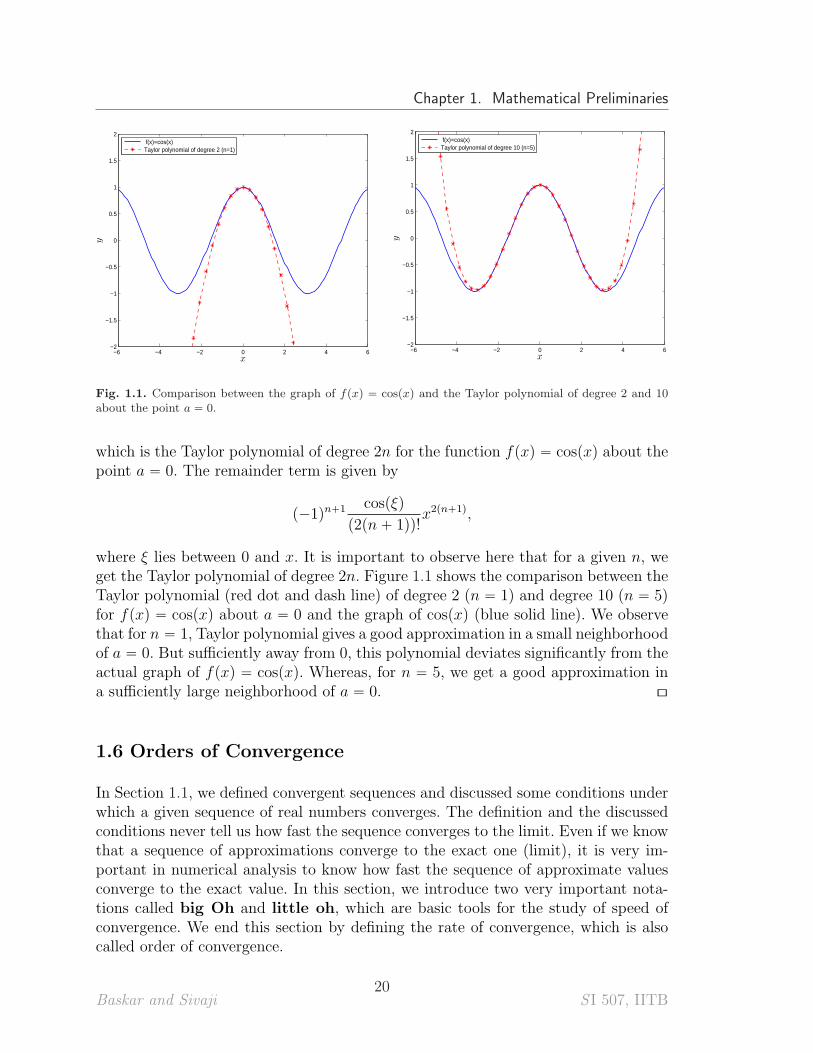
Example 1.36. As another example, let us approximate the function fpxq “ cospxq
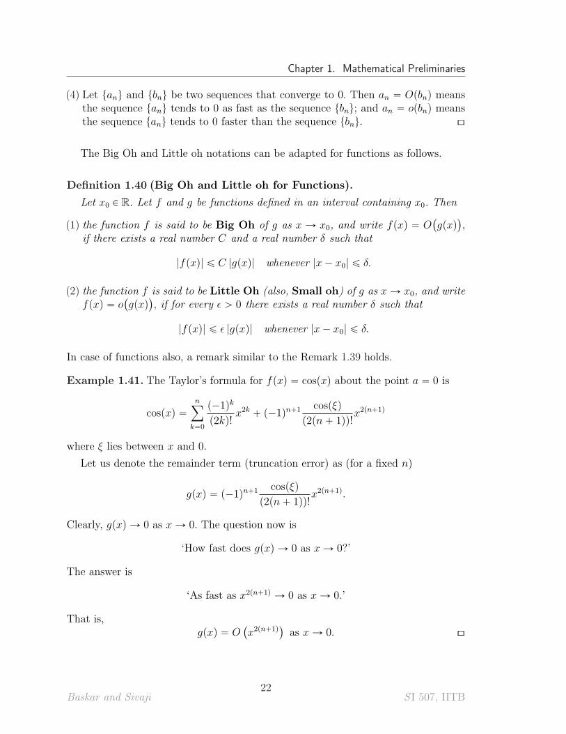
by a polynomial using Taylor’s theorem about the point a “ 0. First, let us take theTaylor’s series expansion
fpxq “ cosp0q ´ sinp0qx ´cosp0q
2!x2 `
sinp0q
3!x3 ` ¨ ¨ ¨
“
8ÿ
k“0
p´1qk
p2kq!x2k.
Now, we truncate this infinite series to get an approximate representation of fpxq
in a sufficiently small neighborhood of a “ 0 as
fpxq «
nÿ
k“0
p´1qk
p2kq!x2k,
Baskar and Sivaji19
S I 507, IITB
Chapter 1. Mathematical Preliminaries
−6 −4 −2 0 2 4 6−2
−1.5
−1
−0.5
0
0.5
1
1.5
2
x
y
f(x)=cos(x) Taylor polynomial of degree 2 (n=1)
−6 −4 −2 0 2 4 6−2
−1.5
−1
−0.5
0
0.5
1
1.5
2
x
y
f(x)=cos(x) Taylor polynomial of degree 10 (n=5)
Fig. 1.1. Comparison between the graph of fpxq “ cospxq and the Taylor polynomial of degree 2 and 10about the point a “ 0.
which is the Taylor polynomial of degree 2n for the function fpxq “ cospxq about thepoint a “ 0. The remainder term is given by
p´1qn`1 cospξq
p2pn ` 1qq!x2pn`1q,
where ξ lies between 0 and x. It is important to observe here that for a given n, weget the Taylor polynomial of degree 2n. Figure 1.1 shows the comparison between theTaylor polynomial (red dot and dash line) of degree 2 (n “ 1) and degree 10 (n “ 5)for fpxq “ cospxq about a “ 0 and the graph of cospxq (blue solid line). We observethat for n “ 1, Taylor polynomial gives a good approximation in a small neighborhoodof a “ 0. But sufficiently away from 0, this polynomial deviates significantly from theactual graph of fpxq “ cospxq. Whereas, for n “ 5, we get a good approximation ina sufficiently large neighborhood of a “ 0. [\
1.6 Orders of Convergence
In Section 1.1, we defined convergent sequences and discussed some conditions underwhich a given sequence of real numbers converges. The definition and the discussedconditions never tell us how fast the sequence converges to the limit. Even if we knowthat a sequence of approximations converge to the exact one (limit), it is very im-portant in numerical analysis to know how fast the sequence of approximate valuesconverge to the exact value. In this section, we introduce two very important nota-tions called big Oh and little oh, which are basic tools for the study of speed ofconvergence. We end this section by defining the rate of convergence, which is alsocalled order of convergence.
Baskar and Sivaji20
S I 507, IITB
Section 1.6. Orders of Convergence
1.6.1 Big Oh and Little oh Notations
The notions of big Oh and little oh are well understood through the following example.
Example 1.37. Consider the two sequences tnu and tn2u both of which are un-bounded and tend to infinity as n Ñ 8. However we feel that the sequence tnu grows‘slowly’ compared to the sequence tn2u. Consider also the sequences t1{nu and t1{n2u
both of which decrease to zero as n Ñ 8. However we feel that the sequence t1{n2u
decreases more rapidly compared to the sequence t1{nu. [\
The above examples motivate us to develop tools that compare two sequences tanu
and tbnu. Landau has introduced the concepts of Big Oh and Little oh for comparingtwo sequences that we will define below.
Definition 1.38 (Big Oh and Little oh).
Let tanu and tbnu be sequences of real numbers. Then
(1) the sequence tanu is said to be Big Oh of tbnu, and write an “ Opbnq, if thereexists a real number C and a natural number N such that
|an| ď C |bn| for all n ě N.
(2) the sequence tanu is said to be Little oh (sometimes said to be small oh) of tbnu,and write an “ opbnq, if for every ϵ ą 0 there exists a natural number N such that
|an| ď ϵ |bn| for all n ě N.
Remark 1.39.
(1) If bn ‰ 0 for every n, then we have an “ Opbnq if and only if the sequence
"
anbn
*
is bounded. That is, there exists a constant C such thatˇ
ˇ
ˇ
ˇ
anbn
ˇ
ˇ
ˇ
ˇ
ď C
(2) If bn ‰ 0 for every n, then we have an “ opbnq if and only if the sequence
"
anbn
*
converges to 0. That is,
limnÑ8
anbn
“ 0.
(3) For any pair of sequences tanu and tbnu such that an “ opbnq, it follows that an “
Opbnq. The converse is not true. Consider the sequences an “ n and bn “ 2n ` 3,for which an “ Opbnq holds but an “ opbnq does not hold.
Baskar and Sivaji21
S I 507, IITB
Chapter 1. Mathematical Preliminaries
(4) Let tanu and tbnu be two sequences that converge to 0. Then an “ Opbnq meansthe sequence tanu tends to 0 as fast as the sequence tbnu; and an “ opbnq meansthe sequence tanu tends to 0 faster than the sequence tbnu. [\
The Big Oh and Little oh notations can be adapted for functions as follows.
Definition 1.40 (Big Oh and Little oh for Functions).
Let x0 P R. Let f and g be functions defined in an interval containing x0. Then
(1) the function f is said to be Big Oh of g as x Ñ x0, and write fpxq “ O`
gpxq˘
,if there exists a real number C and a real number δ such that
|fpxq| ď C |gpxq| whenever |x ´ x0| ď δ.
(2) the function f is said to be Little Oh (also, Small oh) of g as x Ñ x0, and writefpxq “ o
`
gpxq˘
, if for every ϵ ą 0 there exists a real number δ such that
|fpxq| ď ϵ |gpxq| whenever |x ´ x0| ď δ.
In case of functions also, a remark similar to the Remark 1.39 holds.
Example 1.41. The Taylor’s formula for fpxq “ cospxq about the point a “ 0 is
cospxq “
nÿ
k“0
p´1qk
p2kq!x2k ` p´1qn`1 cospξq
p2pn ` 1qq!x2pn`1q
where ξ lies between x and 0.
Let us denote the remainder term (truncation error) as (for a fixed n)
gpxq “ p´1qn`1 cospξq
p2pn ` 1qq!x2pn`1q.
Clearly, gpxq Ñ 0 as x Ñ 0. The question now is
‘How fast does gpxq Ñ 0 as x Ñ 0?’
The answer is
‘As fast as x2pn`1q Ñ 0 as x Ñ 0.’
That is,gpxq “ O
`
x2pn`1q˘
as x Ñ 0. [\
Baskar and Sivaji22
S I 507, IITB
Section 1.6. Orders of Convergence
1.6.2 Rates of Convergence
Let tanu be a sequence such that
limnÑ8
an “ a.
We would like to measure the speed at which the convergence takes place. For exam-ple, consider
limnÑ8
1
2n ` 3“ 0
and
limnÑ8
1
n2“ 0.
We feel that the first sequence goes to zero linearly and the second goes with a muchsuperior speed because of the presence of n2 in its denominator. We will define thenotion of order of convergence precisely.
Definition 1.42 (Rate of Convergence or Order of Convergence).
Let tanu be a sequence such that limnÑ8
an “ a.
(1)We say that the rate of convergence is atleast linear if there exists a constantc ă 1 and a natural number N such that
|an`1 ´ a| ď c |an ´ a| for all n ě N.
(2)We say that the rate of convergence is atleast superlinear if there exists asequence tϵnu that converges to 0, and a natural number N such that
|an`1 ´ a| ď ϵn |an ´ a| for all n ě N.
(3)We say that the rate of convergence is at least quadratic if there exists a constantC (not necessarily less than 1), and a natural number N such that
|an`1 ´ a| ď C |an ´ a|2 for all n ě N.
(4) Let α P R`. We say that the rate of convergence is atleast α if there exists aconstant C (not necessarily less than 1), and a natural number N such that
|an`1 ´ a| ď C |an ´ a|α for all n ě N.
Baskar and Sivaji23
S I 507, IITB
Chapter 1. Mathematical Preliminaries
1.7 Exercises
Sequences of Real Numbers
(1) Consider the sequences tanu and tbnu, where
an “1
n, bn “
1
n2, n “ 1, 2, ¨ ¨ ¨ .
Clearly, both the sequences converge to zero. For the given ϵ “ 10´2, obtain thesmallest positive integers Na and Nb such that
|an| ă ϵ whenever n ě Na, and |bn| ă ϵ whenever n ě Nb.
For any ϵ ą 0, show that Na ą Nb.
(2) Show that the sequence
"
p´1qn `1
n
*
is bounded but not convergent. Observe
that the sequence
"
1 `1
2n
*
is a subsequence of the given sequence. Show that
this subsequence converges and obtain the limit of this subsequence. Obtain an-other convergent subsequence.
(3) Let txnu and tynu be two sequences such that xn, yn P ra, bs and xn ă yn for eachn “ 1, 2, ¨ ¨ ¨ . If xn Ñ b as n Ñ 8, then show that the sequence tynu converges.Find the limit of the sequence tynu.
(4) Let In “
„
n ´ 2
2n,n ` 2
2n
ȷ
, n “ 1, 2, ¨ ¨ ¨ and tanu be a sequence with an is chosen
arbitrarily in In for each n “ 1, 2, ¨ ¨ ¨ . Show that an Ñ1
2as n Ñ 8.
Limits and Continuity
(5) Let
fpxq “
"
sinpxq ´ 1 if x ă 0sinpxq ` 1 if x ą 0
.
Obtain the left hand and right hand limits of f at x “ 0. Does the limit of fexists at x “ 0? Justify your answer.
(6) Let f be a real-valued function such that fpxq ě sinpxq for all x P R. IflimxÑ0
fpxq “ L exists, then show that L ě 0.
Baskar and Sivaji24
S I 507, IITB
Section 1.7. Exercises
(7) Let f , g and h be real-valued functions such that fpxq ď gpxq ď hpxq for all x P R.If x˚ P R is a common root of the equations fpxq “ 0 and hpxq “ 0, then showthat x˚ is a root of the equation gpxq “ 0.
(8) Let P and Q be polynomials. Find
limxÑ8
P pxq
Qpxqand lim
xÑ0
P pxq
Qpxq
in each of the following cases.
(i) The degree of P is less than the degree of Q.
(ii) The degree of P is greater than the degree of Q.
(iii) The agree of P is equal to the degree of Q.
(9) Study the continuity of f in each of the following cases:
(i) fpxq “
"
x2 if x ă 1?x if x ě 1
(ii) fpxq “
"
´x if x ă 1x if x ě 1
(iii) fpxq “
"
0 if x is rational1 if x is irrational
(10) Let f be defined on an interval pa, bq and suppose that f is continuous at c P pa, bqand fpcq ‰ 0. Then, show that there exists a δ ą 0 such that f has the same signas fpcq in the interval pc ´ δ, c ` δq.
(11) Show that the equation sinx`x2 “ 1 has at least one solution in the interval r0, 1s.
(12) Show that pa`bq{2 belongs to the range of the function fpxq “ px´aq2px´bq2`xdefined on the interval ra, bs.
(13) Let fpxq be continuous on ra, bs, let x1, ¨ ¨ ¨ , xn be points in ra, bs, and let g1, ¨ ¨ ¨ ,gn be real numbers having same sign. Show that
nÿ
i“1
fpxiqgi “ fpξq
nÿ
i“1
gi, for some ξ P ra, bs.
(14) Let f : r0, 1s Ñ r0, 1s be a continuous function. Prove that the equation fpxq “ xhas at least one solution lying in the interval r0, 1s (Note: A solution of this equa-tion is called a fixed point of the function f).
Baskar and Sivaji25
S I 507, IITB
Chapter 1. Mathematical Preliminaries
(15) Show that the equation fpxq “ x, where
fpxq “ sin
ˆ
πx ` 1
2
˙
, x P r´1, 1s
has at least one solution in r´1, 1s.
Differentiation
(16) Let c P pa, bq and f : pa, bq Ñ R be differentiable at c. If c is a local extremum(maximum or minimum) of f , then show that f 1pcq “ 0.
(17) Let fpxq “ 1 ´ x2{3. Show that fp1q “ fp´1q “ 0, but that f 1pxq is never zero inthe interval r´1, 1s. Explain how this is possible, in view of Rolle’s theorem.
(18) Let g be a continuous differentiable function (C1 function) such that the equationgpxq “ 0 has at least n roots. Show that the equation g1pxq “ 0 has at least n´ 1roots.
(19) Suppose f is differentiable in an open interval pa, bq. Prove the following state-ments(a) If f 1pxq ě 0 for all x P pa, bq, then f is non-decreasing.(b) If f 1pxq “ 0 for all x P pa, bq, then f is constant.(c) If f 1pxq ď 0 for all x P pa, bq, then f is non-increasing.
(20) Let f : ra, bs Ñ R be given by fpxq “ x2. Find a point c specified by the mean-value theorem for derivatives. Verify that this point lies in the interval pa, bq.
Integration
(21) Prove the second mean value theorem for integrals. Does the theorem hold if thehypothesis gpxq ě 0 for all x P R is replaced by gpxq ď 0 for all x P R.
(22) In the second mean-value theorem for integrals, let fpxq “ ex, gpxq “ x, x P r0, 1s.Find the point c specified by the theorem and verify that this point lies in theinterval p0, 1q.
(23) Let g : r0, 1s Ñ R be a continuous function. Show that there exists a c P p0, 1q
such that1ż
0
x2p1 ´ xq2gpxqdx “1
30gpξq.
Baskar and Sivaji26
S I 507, IITB
Section 1.7. Exercises
(24) If n is a positive integer, show that
?pn`1qπż
?nπ
sinpt2q dt “p´1qn
c,
where?nπ ď c ď
a
pn ` 1qπ.
Taylor’s Theorem
(25) Find the Taylor’s polynomial of degree 2 for the function
fpxq “?x ` 1
about the point a “ 1. Also find the remainder.
(26) Use Taylor’s formula about a “ 0 to evaluate approximately the value of the func-tion fpxq “ ex at x “ 0.5 using three terms (i.e., n “ 2) in the formula. Obtainthe remainder R2p0.5q in terms of the unknown c. Compute approximately thepossible values of c and show that these values lie in the interval p0, 0.5q.
(27) Obtain Taylor expansion for the function fpxq “ sinpxq about the point a “ 0when n “ 1 and n “ 5. Give the reminder term in both the cases.
Big Oh, Little oh, and Orders of convergence
(28) Prove or disprove:
(i) 2n2 ` 3n ` 4 “ opnq as n Ñ 8.
(ii) n`1n2 “ op 1
nq as n Ñ 8.
(iii) n`1n2 “ Op 1
nq as n Ñ 8.
(iv) n`1?n
“ op1q as n Ñ 8.
(v) 1lnn
“ op 1n
q as n Ñ 8.
(vi) 1n lnn
“ op 1n
q as n Ñ 8.
(vii) en
n5 “ Op 1n
q as n Ñ 8.
(29) Prove or disprove:
(i) ex ´ 1 “ Opx2q as x Ñ 0.
(ii) x´2 “ Opcotxq as x Ñ 0.
Baskar and Sivaji27
S I 507, IITB
Chapter 1. Mathematical Preliminaries
(iii) cotx “ opx´1q as x Ñ 0.
(iv) For r ą 0, xr “ Opexq as x Ñ 8.
(v) For r ą 0, lnx “ Opxrq as x Ñ 8.
(30) Assume that fphq “ pphq ` Ophnq and gphq “ qphq ` Ophmq, for some positiveintegers n and m. Find the order of approximation of their sum, ie., find thelargest integer r such that
fphq ` gphq “ pphq ` qphq ` Ophrq.
Baskar and Sivaji28
S I 507, IITB
CHAPTER 2
Error Analysis
Numerical analysis deals with developing methods, called numerical methods, to ap-proximate a solution of a given Mathematical problem (whenever a solution exists).The approximate solution obtained by this method will involve an error which is pre-cisely the difference between the exact solution and the approximate solution. Thus,we have
Exact Solution “ Approximate Solution ` Error.
We call this error the mathematical error.
The study of numerical methods is incomplete if we don’t develop algorithms andimplement the algorithms as computer codes. The outcome of the computer codeis a set of numerical values to the approximate solution obtained using a numericalmethod. Such a set of numerical values is called the numerical solution to the givenMathematical problem. During the process of computation, the computer introducesa new error, called the arithmetic error and we have
Approximate Solution “ Numerical Solution ` Arithmetic Error.
The error involved in the numerical solution when compared to the exact solutioncan be worser than the mathematical error and is now given by
Exact Solution “ Numerical Solution ` Mathematical Error ` Arithmetic Error.
The Total Error is defined as
Total Error “ Mathematical Error ` Arithmetic Error.
A digital calculating device can hold only a finite number of digits because ofmemory restrictions. Therefore, a number cannot be stored exactly. Certain approx-imation needs to be done, and only an approximate value of the given number willfinally be stored in the device. For further calculations, this approximate value isused instead of the exact value of the number. This is the source of arithmetic error.
In this chapter, we introduce the floating-point representation of a real numberand illustrate a few ways to obtain floating-point approximation of a given real num-ber. We further introduce different types of errors that we come across in numerical
Chapter 2. Error Analysis
analysis and their effects in the computation. At the end of this chapter, we will befamiliar with the arithmetic errors, their effect on computed results and some waysto minimize this error in the computation.
2.1 Floating-Point Representation
Let β P N and β ě 2. Any real number can be represented exactly in base β as
p´1qs ˆ p.d1d2 ¨ ¨ ¨ dndn`1 ¨ ¨ ¨ qβ ˆ βe, (2.1.1)
where di P t 0, 1, ¨ ¨ ¨ , β ´ 1 u with d1 ‰ 0 or d1 “ d2 “ d3 “ ¨ ¨ ¨ “ 0, s “ 0 or 1, andan appropriate integer e called the exponent. Here
p.d1d2 ¨ ¨ ¨ dndn`1 ¨ ¨ ¨ qβ “d1β
`d2β2
` ¨ ¨ ¨ `dnβn
`dn`1
βn`1` ¨ ¨ ¨ (2.1.2)
is a β-fraction called the mantissa, s is called the sign and the number β is calledthe radix. The representation (2.1.1) of a real number is called the floating-pointrepresentation.
Remark 2.1. When β “ 2, the floating-point representation (2.1.1) is called thebinary floating-point representation and when β “ 10, it is called the decimalfloating-point representation. Throughout this course, we always take β “ 10.[\
Due to memory restrictions, a computing device can store only a finite number ofdigits in the mantissa. In this section, we introduce the floating-point approximationand discuss how a given real number can be approximated.
2.1.1 Floating-Point Approximation
A computing device stores a real number with only a finite number of digits in themantissa. Although different computing devices have different ways of representingthe numbers, here we introduce a mathematical form of this representation, whichwe will use throughout this course.
Definition 2.2 (n-Digit Floating-point Number).
Let β P N and β ě 2. An n-digit floating-point number in base β is of the form
p´1qs ˆ p.d1d2 ¨ ¨ ¨ dnqβ ˆ βe (2.1.3)
where
p.d1d2 ¨ ¨ ¨ dnqβ “d1β
`d2β2
` ¨ ¨ ¨ `dnβn
(2.1.4)
where di P t 0, 1, ¨ ¨ ¨ , β ´ 1 u with d1 ‰ 0 or d1 “ d2 “ d3 “ ¨ ¨ ¨ “ 0, s “ 0 or 1, andan appropriate exponent e.
Baskar and Sivaji30
S I 507, IITB

Section 2.1. Floating-Point Representation
Remark 2.3. When β “ 2, the n-digit floating-point representation (2.1.3) is calledthe n-digit binary floating-point representation and when β “ 10, it is calledthe n-digit decimal floating-point representation. [\
Example 2.4. The following are examples of real numbers in the decimal floatingpoint representation.
(1) The real number x “ 6.238 is represented in the decimal floating-point represen-tation as
6.238 “ p´1q0 ˆ 0.6238 ˆ 101,
in which case, we have s “ 0, β “ 10, e “ 1, d1 “ 6, d2 “ 2, d3 “ 3 and d4 “ 8.
(2) The real number x “ ´0.0014 is represented in the decimal floating-point repre-sentation as
x “ p´1q1 ˆ 0.14 ˆ 10´2.
Here s “ 1, β “ 10, e “ ´2, d1 “ 1 and d2 “ 4. [\
Remark 2.5. The floating-point representation of the number 1{3 is
1
3“ 0.33333 ¨ ¨ ¨ “ p´1q0 ˆ p0.33333 ¨ ¨ ¨ q10 ˆ 100.
An n-digit decimal floating-point representation of this number has to contain onlyn digits in its mantissa. Therefore, the representation (2.1.3) is (in general) only anapproximation to a real number. [\
Any computing device has its own memory limitations in storing a real number.In terms of the floating-point representation, these limitations lead to the restrictionsin the number of digits in the mantissa (n) and the range of the exponent (e). Insection 2.1.2, we introduce the concept of under and over flow of memory, which is aresult of the restriction in the exponent. The restriction on the length of the mantissais discussed in section 2.1.3.
2.1.2 Underflow and Overflow of Memory
When the value of the exponent e in a floating-point number exceeds the maximumlimit of the memory, we encounter the overflow of memory, whereas when this valuegoes below the minimum of the range, then we encounter underflow. Thus, for agiven computing device, there are real numbers m and M such that the exponent eis limited to a range
m ă e ă M. (2.1.5)
During the calculation, if some computed number has an exponent e ą M then wesay, the memory overflow occurs and if e ă m, we say the memory underflowoccurs.
Baskar and Sivaji31
S I 507, IITB
Chapter 2. Error Analysis
Remark 2.6. In the case of overflow of memory in a floating-point number, a com-puter will usually produce meaningless results or simply prints the symbol inf or NaN.When your computation involves an undetermined quantity (like 0ˆ8, 8´ 8, 0{0),then the output of the computed value on a computer will be the symbol NaN (means‘not a number’). For instance, if X is a sufficiently large number that results in anoverflow of memory when stored on a computing device, and x is another numberthat results in an underflow, then their product will be returned as NaN.
On the other hand, we feel that the underflow is more serious than overflow in acomputation. Because, when underflow occurs, a computer will simply consider thenumber as zero without any warning. However, by writing a separate subroutine, onecan monitor and get a warning whenever an underflow occurs. [\
Example 2.7 (Overflow). Run the following MATLAB code on a computer with32-bit intel processor:
i=308.25471;
fprintf(’%f %f\n’,i,10^i);
i=308.25472;
fprintf(’%f %f\n’,i,10^i);
We see that the first print command shows a meaningful (but very large) number,whereas the second print command simply prints inf. This is due to the overflow ofmemory while representing a very large real number.
Also try running the following code on the MATLAB:
i=308.25471;
fprintf(’%f %f\n’,i,10^i/10^i);
i=308.25472;
fprintf(’%f %f\n’,i,10^i/10^i);
The output will be
308.254710 1.000000
308.254720 NaN
If your computer is not showing inf for i = 308.25472, try increasing the value ofi till you get inf. [\
Example 2.8 (Underflow). Run the following MATLAB code on a computer with32-bit intel processor:
j=-323.6;
if(10^j>0)
Baskar and Sivaji32
S I 507, IITB
Section 2.1. Floating-Point Representation
fprintf(’The given number is greater than zero\n’);
elseif (10^j==0)
fprintf(’The given number is equal to zero\n’);
else
fprintf(’The given number is less than zero\n’);
end
The output will be
The given number is greater than zero
When the value of j is further reduced slightly as shown in the following program
j=-323.64;
if(10^j>0)
fprintf(’The given number is greater than zero\n’);
elseif (10^j==0)
fprintf(’The given number is equal to zero\n’);
else
fprintf(’The given number is less than zero\n’);
end
the output shows
The given number is equal to zero
If your computer is not showing the above output, try decreasing the value of j tillyou get the above output.
In this example, we see that the number 10´323.64 is recognized as zero by thecomputer. This is due to the underflow of memory. Note that multiplying any largenumber by this number will give zero as answer. If a computation involves such anunderflow of memory, then there is a danger of having a large difference between theactual value and the computed value. [\
2.1.3 Chopping and Rounding a Number
The number of digits in the mantissa, as given in Definition 2.2, is called the precisionor length of the floating-point number. In general, a real number can have infinitelymany digits, which a computing device cannot hold in its memory. Rather, eachcomputing device will have its own limitation on the length of the mantissa. If agiven real number has infinitely many digits in the mantissa of the floating-pointform as in (2.1.1), then the computing device converts this number into an n-digitfloating-point form as in (2.1.3). Such an approximation is called the floating-pointapproximation of a real number.
Baskar and Sivaji33
S I 507, IITB
Chapter 2. Error Analysis
There are many ways to get floating-point approximation of a given real number.Here we introduce two types of floating-point approximation.
Definition 2.9 (Chopped and Rounded Numbers).
Let x be a real number given in the floating-point representation (2.1.1) as
x “ p´1qs ˆ p.d1d2 ¨ ¨ ¨ dndn`1 ¨ ¨ ¨ qβ ˆ βe.
The floating-point approximation of x using n-digit chopping is given by
flpxq “ p´1qs ˆ p.d1d2 ¨ ¨ ¨ dnqβ ˆ βe. (2.1.6)
The floating-point approximation of x using n-digit rounding is given by
flpxq “
"
p´1qs ˆ p.d1d2 ¨ ¨ ¨ dnqβ ˆ βe , 0 ď dn`1 ăβ2
p´1qs ˆ p.d1d2 ¨ ¨ ¨ pdn ` 1qqβ ˆ βe , β2
ď dn`1 ă β, (2.1.7)
where
p´1qs ˆ p.d1d2 ¨ ¨ ¨ pdn ` 1qqβ ˆβe :“ p´1qs ˆ
¨
˝p.d1d2 ¨ ¨ ¨ dnqβ ` p. 0 0 ¨ ¨ ¨ 0looomooon
pn´1q´times
1qβ
˛
‚ˆβe.
As already mentioned, throughout this course, we always take β “ 10. Also, we donot assume any restriction on the exponent e P Z.
Example 2.10. The floating-point representation of π is given by
π “ p´1q0 ˆ p.31415926 ¨ ¨ ¨ q ˆ 101.
The floating-point approximation of π using five-digit chopping is
flpπq “ p´1q0 ˆ p.31415q ˆ 101,
which is equal to 3.1415. Since the sixth digit of the mantissa in the floating-pointrepresentation of π is a 9, the floating-point approximation of π using five-digitrounding is given by
flpπq “ p´1q0 ˆ p.31416q ˆ 101,
which is equal to 3.1416. [\
Remark 2.11.Most of the modern processors, including Intel, uses IEEE 754 stan-dard format. This format uses 52 bits in mantissa, (64-bit binary representation), 11bits in exponent and 1 bit for sign. This representation is called the double precisionnumber.
When we perform a computation without any floating-point approximation, wesay that the computation is done using infinite precision (also called exact arith-metic). [\
Baskar and Sivaji34
S I 507, IITB
Section 2.1. Floating-Point Representation
2.1.4 Arithmetic Using n-Digit Rounding and Chopping
In this subsection, we describe the procedure of performing arithmetic operationsusing n-digit rounding. The procedure of performing arithmetic operation using n-digit chopping is done in a similar way.
Let d denote any one of the basic arithmetic operations ‘`’, ‘´’, ‘ˆ’ and ‘˜’. Letx and y be real numbers. The process of computing x d y using n-digit roundingis as follows.
Step 1: Get the n-digit rounding approximation flpxq and flpyq of the numbers x andy, respectively.
Step 2: Perform the calculation flpxq d flpyq using exact arithmetic.
Step 3: Get the n-digit rounding approximation flpflpxq d flpyqq of flpxq d flpyq.
The result from step 3 is the value of x d y using n-digit rounding.
Example 2.12. Consider the function
fpxq “ x´?
x ` 1 ´?x¯
.
Let us evaluate fp100000q using a six-digit rounding. We have
fp100000q “ 100000´?
100001 ´?100000
¯
.
The evaluation of?100001 using six-digit rounding is as follows.
?100001 « 316.229347
“ 0.316229347 ˆ 103.
The six-digit rounded approximation of 0.316229347ˆ103 is given by 0.316229ˆ103.Therefore,
flp?100001q “ 0.316229 ˆ 103.
Similarly,flp
?100000q “ 0.316228 ˆ 103.
The six-digit rounded approximation of the difference between these two numbers is
fl´
flp?100001q ´ flp
?100000q
¯
“ 0.1 ˆ 10´2.
Finally, we have
flpfp100000qq “ flp100000q ˆ p0.1 ˆ 10´2q
“ p0.1 ˆ 106q ˆ p0.1 ˆ 10´2q
“ 100.
Using six-digit chopping, the value of flpfp100000qq is 200. [\
Baskar and Sivaji35
S I 507, IITB
Chapter 2. Error Analysis
Definition 2.13 (Machine Epsilon).
The machine epsilon of a computer is the smallest positive floating-point number δsuch that
flp1 ` δq ą 1.
For any floating-point number δ ă δ, we have flp1 ` δq “ 1, and 1 ` δ and 1 areidentical within the computer’s arithmetic.
Remark 2.14. From Example 2.8, it is clear that the machine epsilon for a 32-bitintel processor lies between the numbers 10´323.64 and 10´323.6. It is possible to getthe exact value of this number, but it is no way useful in our present course, and sowe will not attempt to do this here. [\
2.2 Types of Errors
The approximate representation of a real number obviously differs from the actualnumber, whose difference is called an error.
Definition 2.15 (Errors).
(1) The error in a computed quantity is defined as
Error = True Value - Approximate Value.
(2) Absolute value of an error is called the absolute error.
(3) The relative error is a measure of the error in relation to the size of the truevalue as given by
Relative Error “Error
True Value.
Here, we assume that the true value is non-zero.
(4) The percentage error is defined as
Percentage Error “ 100 ˆ |Relative Error|.
Remark 2.16. Let xA denote the approximation to the real number x. We use thefollowing notations:
EpxAq :“ ErrorpxAq “ x ´ xA. (2.2.8)
EapxAq :“ Absolute ErrorpxAq “ |EpxAq| (2.2.9)
ErpxAq :“ Relative ErrorpxAq “EpxAq
x, x ‰ 0. (2.2.10)
[\
Baskar and Sivaji36
S I 507, IITB
Section 2.3. Loss of Significance
The absolute error has to be understood more carefully because a relatively smalldifference between two large numbers can appear to be large, and a relatively largedifference between two small numbers can appear to be small. On the other hand,the relative error gives a percentage of the difference between two numbers, which isusually more meaningful as illustrated below.
Example 2.17. Let x “ 100000, xA “ 99999, y “ 1 and yA “ 1{2. We have
EapxAq “ 1, EapyAq “1
2.
Although EapxAq ą EapyAq, we have
ErpxAq “ 10´5, ErpyAq “1
2.
Hence, in terms of percentage error, xA has only 10´3% error when compared to xwhereas yA has 50% error when compared to y. [\
The errors defined above are between a given number and its approximate value.Quite often we also approximate a given function by another function that can behandled more easily. For instance, a sufficiently differentiable function can be approx-imated using Taylor’s theorem 1.29. The error between the function value and thevalue obtained from the corresponding Taylor’s polynomial is defined as Truncationerror as defined in Definition 1.32.
2.3 Loss of Significance
In place of relative error, we often use the concept of significant digits that is closelyrelated to relative error.
Definition 2.18 (Significant β-Digits).
Let β be a radix and x ‰ 0. If xA is an approximation to x, then we say that xAapproximates x to r significant β-digits if r is the largest non-negative integer suchthat
|x ´ xA|
|x|ď
1
2β´r`1. (2.3.11)
We also say xA has r significant β-digits in x. [\
Remark 2.19. When β “ 10, we refer significant 10-digits by significant digits. [\
Baskar and Sivaji37
S I 507, IITB
Chapter 2. Error Analysis
Example 2.20.
(1) For x “ 1{3, the approximate number xA “ 0.333 has three significant digits,since
|x ´ xA|
|x|“ 0.001 ă 0.005 “ 0.5 ˆ 10´2.
Thus, r “ 3.
(2) For x “ 0.02138, the approximate number xA “ 0.02144 has three significantdigits, since
|x ´ xA|
|x|« 0.0028 ă 0.005 “ 0.5 ˆ 10´2.
Thus, r “ 3.
(3) For x “ 0.02132, the approximate number xA “ 0.02144 has two significant digits,since
|x ´ xA|
|x|« 0.0056 ă 0.05 “ 0.5 ˆ 10´1.
Thus, r “ 2.
(4) For x “ 0.02138, the approximate number xA “ 0.02149 has two significant digits,since
|x ´ xA|
|x|« 0.0051 ă 0.05 “ 0.5 ˆ 10´1.
Thus, r “ 2.
(5) For x “ 0.02108, the approximate number xA “ 0.0211 has three significant digits,since
|x ´ xA|
|x|« 0.0009 ă 0.005 “ 0.5 ˆ 10´2.
Thus, r “ 3.
(6) For x “ 0.02108, the approximate number xA “ 0.02104 has three significantdigits, since
|x ´ xA|
|x|« 0.0019 ă 0.005 “ 0.5 ˆ 10´2.
Thus, r “ 3. [\
Remark 2.21. Number of significant digits roughly measures the number of leadingnon-zero digits of xA that are correct relative to the corresponding digits in the truevalue x. However, this is not a precise way to get the number of significant digits asit is evident from the above examples. [\
The role of significant digits in numerical calculations is very important in thesense that the loss of significant digits may result in drastic amplification of therelative error as illustrated in the following example.
Baskar and Sivaji38
S I 507, IITB
Section 2.3. Loss of Significance
Example 2.22. Let us consider two real numbers
x “ 7.6545428 “ 0.76545428 ˆ 101 and y “ 7.6544201 “ 0.76544201 ˆ 101.
The numbers
xA “ 7.6545421 “ 0.76545421 ˆ 101 and yA “ 7.6544200 “ 0.76544200 ˆ 101
are approximations to x and y, correct to seven and eight significant digits, respec-tively. The exact difference between xA and yA is
zA “ xA ´ yA “ 0.12210000 ˆ 10´3
and the exact difference between x and y is
z “ x ´ y “ 0.12270000 ˆ 10´3.
Therefore,|z ´ zA|
|z|« 0.0049 ă 0.5 ˆ 10´2
and hence zA has only three significant digits with respect to z. Thus, we started withtwo approximate numbers xA and yA which are correct to seven and eight significantdigits with respect to x and y respectively, but their difference zA has only threesignificant digits with respect to z. Hence, there is a loss of significant digits in theprocess of subtraction. A simple calculation shows that
ErpzAq « 53581 ˆ ErpxAq.
Similarly, we haveErpzAq « 375067 ˆ ErpyAq.
Loss of significant digits is therefore dangerous. The loss of significant digits in theprocess of calculation is referred to as Loss of Significance. [\
Example 2.23. Consider the function
fpxq “ xp?x ` 1 ´
?xq.
From Example 2.12, the value of fp100000q using six-digit rounding is 100, whereasthe true value is 158.113. There is a drastic error in the value of the function, whichis due to the loss of significant digits. It is evident that as x increases, the terms?x ` 1 and
?x comes closer to each other and therefore loss of significance in their
computed value increases.
Such a loss of significance can be avoided by rewriting the given expression off in such a way that subtraction of near-by non-negative numbers is avoided. Forinstance, we can re-write the expression of the function f as
Baskar and Sivaji39
S I 507, IITB
Chapter 2. Error Analysis
fpxq “x
?x ` 1 `
?x.
With this new form of f , we obtain fp100000q “ 158.114000 using six-digit rounding.[\
Example 2.24. Consider evaluating the function
fpxq “ 1 ´ cos x
near x “ 0. Since cos x « 1 for x near zero, there will be loss of significance in theprocess of evaluating fpxq for x near zero. So, we have to use an alternative formulafor fpxq such as
fpxq “ 1 ´ cosx
“1 ´ cos2 x
1 ` cosx
“sin2 x
1 ` cos x
which can be evaluated quite accurately for small x. [\
Remark 2.25. Unlike the above examples, we may not be able to write an equivalentformula for the given function to avoid loss of significance in the evaluation. In suchcases, we have to go for a suitable approximation of the given function by otherfunctions, for instance Taylor’s polynomial of desired degree, that do not involve lossof significance. [\
2.4 Propagation of Relative Error in Arithmetic Operations
Once an error is committed, it affects subsequent results as this error propagatesthrough subsequent calculations. We first study how the results are affected by usingapproximate numbers instead of actual numbers and then will take up the effect oferrors on function evaluation in the next section.
Let xA and yA denote the approximate numbers used in the calculation, and letxT and yT be the corresponding true values. We will now see how relative errorpropagates with the four basic arithmetic operations.
2.4.1 Addition and Subtraction
Let xT “ xA ` ϵ and yT “ yA ` η be positive real numbers. The relative errorErpxA ˘ yAq is given by
Baskar and Sivaji40
S I 507, IITB
Section 2.4. Propagation of Relative Error in Arithmetic Operations
ErpxA ˘ yAq “pxT ˘ yT q ´ pxA ˘ yAq
xT ˘ yT
“pxT ˘ yT q ´ pxT ´ ϵ ˘ pyT ´ ηqq
xT ˘ yT
Upon simplification, we get
ErpxA ˘ yAq “ϵ ˘ η
xT ˘ yT. (2.4.12)
The above expression shows that there can be a drastic increase in the relative errorduring subtraction of two approximate numbers whenever xT « yT as we have wit-nessed in Examples 2.22 and 2.23. On the other hand, it is easy to see from (2.4.12)that
|ErpxA ` yAq| ď |ErpxAq| ` |ErpyAq|,
which shows that the relative error propagates slowly in addition. Note that such aninequality in the case of subtraction is not possible.
2.4.2 Multiplication
The relative error ErpxA ˆ yAq is given by
ErpxA ˆ yAq “pxT ˆ yT q ´ pxA ˆ yAq
xT ˆ yT
“pxT ˆ yT q ´ ppxT ´ ϵq ˆ pyT ´ ηqq
xT ˆ yT
“ηxT ` ϵyT ´ ϵη
xT ˆ yT
“ϵ
xT`
η
yT´
ˆ
ϵ
xT
˙ˆ
η
yT
˙
Thus, we have
ErpxA ˆ yAq “ ErpxAq ` ErpyAq ´ ErpxAqErpyAq. (2.4.13)
Taking modulus on both sides, we get
|ErpxA ˆ yAq| ď |ErpxAq| ` |ErpyAq| ` |ErpxAq| |ErpyAq|
Note that when |ErpxAq| and |ErpyAq| are very small, then their product is negligiblewhen compared to |ErpxAq| ` |ErpyAq|. Therefore, the above inequality reduces to
|ErpxA ˆ yAq| Æ |ErpxAq| ` |ErpyAq|,
which shows that the relative error propagates slowly in multiplication.
Baskar and Sivaji41
S I 507, IITB
Chapter 2. Error Analysis
2.4.3 Division
The relative error ErpxA{yAq is given by
ErpxA{yAq “pxT {yT q ´ pxA{yAq
xT {yT
“pxT {yT q ´ ppxT ´ ϵq{pyT ´ ηqq
xT {yT
“xT pyT ´ ηq ´ yT pxT ´ ϵq
xT pyT ´ ηq
“ϵyT ´ ηxTxT pyT ´ ηq
“yT
yT ´ ηpErpxAq ´ ErpyAqq
Thus, we have
ErpxA{yAq “1
1 ´ ErpyAqpErpxAq ´ ErpyAqq. (2.4.14)
The above expression shows that the relative error increases drastically during di-vision whenever ErpyAq « 1. This means that yA has 100% error when comparedto y, which is very unlikely because we always expect the relative error to be verysmall, ie., very close to zero. In this case the right hand side is approximately equalto ErpxAq ´ ErpyAq. Hence, we have
|ErpxA{yAq| Æ |ErpxAq ´ ErpyAq| ď |ErpxAq| ` |ErpyAq|,
which shows that the relative error propagates slowly in division.
2.4.4 Total Error
In Subsection 2.1.4, we discussed the procedure of performing arithmetic operationsusing n-digit floating-point approximation. The computed value flpflpxq d flpyqq in-volves an error (when compared to the exact value x d y) which comprises of
(1) Error in flpxq and flpyq due to n-digit rounding or chopping of x and y, respectively,and
(2) Error in flpflpxq dflpyqq due to n-digit rounding or chopping of the number flpxq d
flpyq.
The total error is defined as
pxd yq ´flpflpxq dflpyqq “ rpxd yq ´ pflpxq dflpyqqs ` rpflpxq dflpyqq ´flpflpxq dflpyqqs,
in which the first term on the right hand side is called the propagated error andthe second term is called the floating-point error. The relative total error isobtained by dividing both sides of the above expression by x d y.
Baskar and Sivaji42
S I 507, IITB
Section 2.5. Propagation of Relative Error in Function Evaluation
Example 2.26. Consider evaluating the integral
In “
ż 1
0
xn
x ` 5dx, for n “ 0, 1, ¨ ¨ ¨ , 30.
The value of In can be obtained in two different iterative processes, namely,
(1) The forward iteration for evaluating In is given by
In “1
n´ 5In´1, I0 “ lnp6{5q.
(2) The backward iteration for evaluating In´1 is given by
In´1 “1
5n´
1
5In, I30 “ 0.54046330 ˆ 10´2.
The following table shows the computed value of In using both iterative formulasalong with the exact value. The numbers are computed using MATLAB using doubleprecision arithmetic and the final answer is rounded to 6 digits after the decimalpoint.
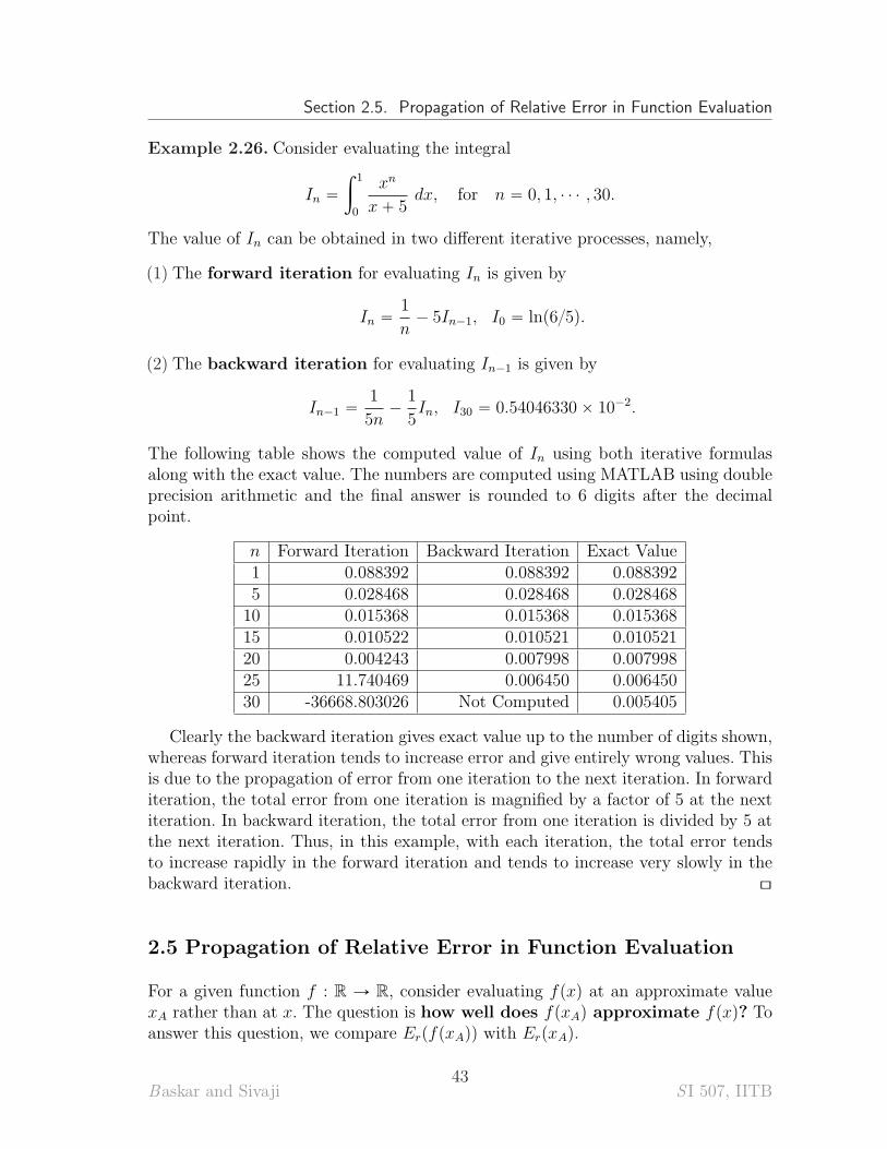
n Forward Iteration Backward Iteration Exact Value1 0.088392 0.088392 0.0883925 0.028468 0.028468 0.02846810 0.015368 0.015368 0.01536815 0.010522 0.010521 0.01052120 0.004243 0.007998 0.00799825 11.740469 0.006450 0.00645030 -36668.803026 Not Computed 0.005405
Clearly the backward iteration gives exact value up to the number of digits shown,whereas forward iteration tends to increase error and give entirely wrong values. Thisis due to the propagation of error from one iteration to the next iteration. In forwarditeration, the total error from one iteration is magnified by a factor of 5 at the nextiteration. In backward iteration, the total error from one iteration is divided by 5 atthe next iteration. Thus, in this example, with each iteration, the total error tendsto increase rapidly in the forward iteration and tends to increase very slowly in thebackward iteration. [\
2.5 Propagation of Relative Error in Function Evaluation
For a given function f : R Ñ R, consider evaluating fpxq at an approximate valuexA rather than at x. The question is how well does fpxAq approximate fpxq? Toanswer this question, we compare ErpfpxAqq with ErpxAq.
Baskar and Sivaji43
S I 507, IITB
Chapter 2. Error Analysis
Assume that f is a C1 function. Using the mean-value theorem, we get
fpxq ´ fpxAq “ f 1pξqpx ´ xAq,
where ξ is an unknown point between x and xA. The relative error in fpxAq whencompared to fpxq is given by
ErpfpxAqq “f 1pξq
fpxqpx ´ xAq.
Thus, we have
ErpfpxAqq “
ˆ
f 1pξq
fpxqx
˙
ErpxAq. (2.5.15)
Since xA and x are assumed to be very close to each other and ξ lies between x andxA, we may make the approximation
fpxq ´ fpxAq « f 1pxqpx ´ xAq.
In view of (2.5.15), we have
ErpfpxAqq «
ˆ
f 1pxq
fpxqx
˙
ErpxAq. (2.5.16)
The expression inside the bracket on the right hand side of (2.5.16) is the amplificationfactor for the relative error in fpxAq in terms of the relative error in xA. Thus, thisexpression plays an important role in understanding the propagation relative errorin evaluating the function value fpxq and hence motivates the following definition.
Definition 2.27 (Condition Number of a Function).
The condition number of a continuously differentiable function f at a point x “ cis given by
ˇ
ˇ
ˇ
ˇ
f 1pcq
fpcqc
ˇ
ˇ
ˇ
ˇ
. (2.5.17)
The condition number of a function at a point x “ c can be used to decide whetherthe evaluation of the function at x “ c is well-conditioned or ill-conditioned depend-ing on whether this condition number is smaller or larger as we approach this point.It is not possible to decide a priori how large the condition number should be to saythat the function evaluation is ill-conditioned and it depends on the circumstancesin which we are working.
Baskar and Sivaji44
S I 507, IITB
Section 2.5. Propagation of Relative Error in Function Evaluation
Definition 2.28 (Well-Conditioned and Ill-Conditioned).
The process of evaluating a continuously differentiable function f at a point x “ c issaid to be well-conditioned if the condition number
ˇ
ˇ
ˇ
ˇ
f 1pcq
fpcqc
ˇ
ˇ
ˇ
ˇ
at c is ‘small’. The process of evaluating a function at x “ c is said to be ill-conditioned if it is not well-conditioned.
Example 2.29. Consider the function fpxq “?x, for all x P r0,8q. Then
f 1pxq “1
2?x, for all x P r0,8q.
The condition number of f is
ˇ
ˇ
ˇ
ˇ
f 1pxq
fpxqx
ˇ
ˇ
ˇ
ˇ
“1
2, for all x P r0,8q
which shows that taking square roots is a well-conditioned process. From (2.5.16), wehave
|ErpfpxAqq| «1
2|ErpxAq|.
Thus, ErpfpxAqq is more closer to zero than ErpxAq. [\
Example 2.30. Consider the function
fpxq “10
1 ´ x2, for all x P R.
Then f 1pxq “ 20x{p1 ´ x2q2, so that
ˇ
ˇ
ˇ
ˇ
f 1pxq
fpxqx
ˇ
ˇ
ˇ
ˇ
“
ˇ
ˇ
ˇ
ˇ
p20x{p1 ´ x2q2qx
10{p1 ´ x2q
ˇ
ˇ
ˇ
ˇ
“2x2
|1 ´ x2|
and this number can be quite large for |x| near 1. Thus, for x near 1 or -1, the processof evaluating this function is ill-conditioned. [\
The above two examples gives us a feeling that if the process of evaluating afunction is well-conditioned, then we tend to get less propagating relative error. But,this is not true in general as shown in the following example.
Baskar and Sivaji45
S I 507, IITB
Chapter 2. Error Analysis
Example 2.31. Consider the function
fpxq “?x ` 1 ´
?x, for all x P p0,8q.
For all x P p0,8q, the condition number of this function is
ˇ
ˇ
ˇ
ˇ
f 1pxq
fpxqx
ˇ
ˇ
ˇ
ˇ
“1
2
ˇ
ˇ
ˇ
ˇ
ˇ
ˇ
ˇ
ˇ
ˆ
1?x ` 1
´1
?x
˙
?x ` 1 ´
?x
x
ˇ
ˇ
ˇ
ˇ
ˇ
ˇ
ˇ
ˇ
“1
2
x?x ` 1
?x
ď1
2, (2.5.18)
which shows that the process of evaluating f is well-conditioned for all x P p0,8q.But, if we calculate fp12345q using six-digit rounding, we find
fp12345q “?12346 ´
?12345 “ 111.113 ´ 111.108 “ 0.005,
while, actually, fp12345q “ 0.00450003262627751 ¨ ¨ ¨ . The calculated answer has 10%error. [\
The above example shows that a well-conditioned process of evaluating a function ata point is not enough to ensure the accuracy in the corresponding computed value. Weneed to check for the stability of the computation, which we discuss in the followingsubsection.
2.5.1 Stable and Unstable Computations
Suppose there are n steps to evaluate a function fpxq at a point x “ c. Then thetotal process of evaluating this function is said to have instability if atleast one ofthe n steps is ill-conditioned. If all the steps are well-conditioned, then the process issaid to be stable.
Example 2.32. We continue the discussion in example 2.31 and check the stabilityin evaluating the function f . Let us analyze the computational process. The functionf consists of the following four computational steps in evaluating the value of f atx “ x0:
x1 :“ x0 ` 1, x2 :“?x1, x3 :“
?x0, x4 :“ x2 ´ x3.
Now consider the last two steps where we already computed x2 and now going tocompute x3 and finally evaluate the function
Baskar and Sivaji46
S I 507, IITB
Section 2.5. Propagation of Relative Error in Function Evaluation
f4ptq :“ x2 ´ t.
At this step, the condition number for f4 is given by
ˇ
ˇ
ˇ
ˇ
f 14ptq
f4ptqt
ˇ
ˇ
ˇ
ˇ
“
ˇ
ˇ
ˇ
ˇ
t
x2 ´ t
ˇ
ˇ
ˇ
ˇ
.
Thus, f4 is ill-conditioned when t approaches x2. Therefore, the above process ofevaluating the function fpxq is unstable.
Let us rewrite the same function fpxq as
fpxq “1
?x ` 1 `
?x.
The computational process of evaluating f at x “ x0 is
x1 :“ x0 ` 1, x2 :“?x1, x3 :“
?x0, x4 :“ x2 ` x3, x5 :“ 1{x4.
It is easy to verify that the condition number of each of the above steps is well-conditioned. For instance, the last step defines
f5ptq “1
x2 ` t,
and the condition number of this function is approximately,
ˇ
ˇ
ˇ
ˇ
ˇ
f 15pxq
f5pxqx
ˇ
ˇ
ˇ
ˇ
ˇ
“
ˇ
ˇ
ˇ
ˇ
t
x2 ` t
ˇ
ˇ
ˇ
ˇ
«1
2
for t sufficiently close to x2. Therefore, this process of evaluating fpxq is stable.Recall from example 2.23 that the above expression gives a more accurate value forsufficiently large x. [\
Remark 2.33. As discussed in Remark 2.25, we may not be lucky all the time tocome out with an alternate expression that lead to stable evaluation for any givenfunction when the original expression leads to unstable evaluation. In such situations,we have to compromise and go for a suitable approximation with other functions withstable evaluation process. For instance, we may try approximating the given functionwith its Taylor’s polynomial, if possible. [\
Baskar and Sivaji47
S I 507, IITB
Chapter 2. Error Analysis
2.6 Exercises
Floating-Point Approximation
(1) Let X be a sufficiently large number which result in an overflow of memory on acomputing device. Let x be a sufficiently small number which result in underflowof memory on the same computing device. Then give the output of the followingoperations:(i) x ˆ X (ii) 3 ˆ X (iii) 3 ˆ x (iv) x{X (v) X{x.
(2) In the following problems, show all the steps involved in the computation.
(i) Using 5-digit rounding, compute 37654 ` 25.874 ´ 37679.
(ii) Let a “ 0.00456, b “ 0.123, c “ ´0.128. Using 3-digit rounding, computepa ` bq ` c, and a ` pb ` cq. What is your conclusion?
(iii) Let a “ 2, b “ ´0.6, c “ 0.602. Using 3-digit rounding, compute a ˆ pb ` cq,and pa ˆ bq ` pa ˆ cq. What is your conclusion?
(3) To find the mid-point of an interval ra, bs, the formula a`b2
is often used. Com-pute the mid-point of the interval r0.982, 0.987s using 3-digit chopping. On thenumber line represent all the three points. What do you observe? Now use themore geometric formula a ` b´a
2to compute the mid-point, once again using 3-
digit chopping. What do you observe this time? Why is the second formula moregeometric?
(4) In a computing device that uses n-digit rounding binary floating-point arithmetic,show that δ “ 2´n is the machine epsilon. What is the machine epsilon in acomputing device that uses n-digit rounding decimal floating-point arithmetic?Justify your answer.
Types of Errors
(5) If flpxq is the approximation of a real number x in a computing device, and ϵ isthe corresponding relative error, then show that flpxq “ p1 ´ ϵqx.
(6) Let x, y and z be real numbers whose floating point approximations in a com-puting device coincide with x, y and z respectively. Show that the relative er-ror in computing xpy ` zq equals ϵ1 ` ϵ2 ´ ϵ1ϵ2, where ϵ1 “ Erpflpy ` zqq andϵ2 “ Erpflpx ˆ flpy ` zqqq.
(7) Let ϵ “ Erpflpxqq. Show that
(i) |ϵ| ď 10´n`1 if the computing device uses n-digit (decimal) chopping.
(ii) |ϵ| ď 1210´n`1 if the computing device uses n-digit (decimal) rounding.
(iii) Can the equality hold in the above inequalities?
Baskar and Sivaji48
S I 507, IITB
Section 2.6. Exercises
(8) For small values of x, the approximation sinx « x is often used. Estimate theerror in using this formula with the aid of Taylor’s theorem. For what range ofvalues of x will this approximation give an absolute error of at most 1
210´6?(Quiz
1, Spring 2011)
(9) Let xA “ 3.14 and yA “ 2.651 be obtained from xT and yT using 4-digit rounding.Find the smallest interval that contains(i) xT (ii) yT (iii) xT ` yT (iv) xT ´ yT (v) xT ˆ yT (vi) xT {yT .
(10) The ideal gas law is given by PV “ nRT where R is the gas constant. We areinterested in knowing the value of T for which P “ V “ n “ 1. If R is known onlyapproximately as RA “ 8.3143 with an absolute error at most 0.12 ˆ 10´2. Whatis the relative error in the computation of T that results in using RA instead of R?
Loss of Significance and Propagation of Error
(11) Obtain the number of significant digits in xA when compared to x for the followingcases:(i) x “ 451.01 and xA “ 451.023 (ii) x “ ´0.04518 and xA “ ´0.045113(iii) x “ 23.4604 and x “ 23.4213.
(12) Instead of using the true values xT “ 0.71456371 and yT “ 0.71456238 in cal-culating zT “ xT ´ yT p“ 0.133 ˆ 10´5q, if we use the approximate values xA “
0.71456414 and yA “ 0.71456103, and calculate zA “ xA´yAp“ 0.311ˆ10´5q, thenfind the loss of significant digits in the process of calculating zA when comparedto the significant digits in xA.
(13) Let x ă 0 ă y be such that the approximate numbers xA and yA has seven andnine significant digits with x and y respectively. Show that zA :“ xA ´ yA has atleast six significant digits when compared to z :“ x ´ y.
Propagation of Relative Error
(14) Let x “ 0.65385 and y “ 0.93263. Obtain the total error in obtaining the productof these two numbers using 3-digit rounding calculation.
(15) Let f : R Ñ R and g : R Ñ R be continuously differentiable functions such that
• there exists constant M ą 0 such that |f 1pxq| ě M and |g1pxq| ď M for allx P R,
• the process of evaluating f is well-conditioned, and
• the process of evaluating g is ill-conditioned.
Show that |gpxq| ă |fpxq| for all x P R. (Mid-Sem, Spring 2011)
Baskar and Sivaji49
S I 507, IITB
Chapter 2. Error Analysis
(16) Find the condition number at a point x “ c for the following functions(i) fpxq “ x2, (ii) gpxq “ πx, (iii) hpxq “ bx.
(17) Let xT be a real number. Let xA “ 2.5 be an approximate value of xT with anabsolute error at most 0.01. The function fpxq “ x3 is evaluated at x “ xA insteadof x “ xT . Estimate the resulting absolute error.
(18) Is the process of computing the function fpxq “ pex ´ 1q{x stable or unstable forx « 0? Justify your answer. (Quiz1, Autumn 2010)
(19) Show that the process of evaluating the function
fpxq “1 ´ cos x
x2
for x « 0 is unstable. Suggest an alternate formula for evaluating f for x « 0,and check if the computation process is stable using this new formula.
(20) Check for stability of computing the function
fpxq “
ˆ
x `1
3
˙
´
ˆ
x ´1
3
˙
for large values of x.
(21) Check for stability of computing the function
gpxq “
ˆ
3 `x2
3
˙
´
ˆ
3 ´x2
3
˙
x2
for values of x very close to 0.
(22) Check for stability of computing the function
hpxq “sin2 x
1 ´ cos2 x
for values of x very close to 0.
(23) Compute the values of the function
sin x?1 ´ sin2 x
using your calculator (without simplifying the given formula) at x “ 89.9, 89.95, 89.99degrees. Also compute the values of the function tanx at these values of x andcompare the number of significant digits.
Baskar and Sivaji50
S I 507, IITB
CHAPTER 3
Numerical Linear Algebra
In this chapter, we study the methods for solving system of linear equations, andcomputing an eigenvalue and the corresponding eigen vector for a matrix. The meth-ods for solving linear systems is categorized into two types, namely, direct methodsand iterative methods. Theoretically, direct methods give exact solution of a lin-ear system and therefore these methods do not involve mathematical error. However,when we implement the direct methods on a computer, because of the presence ofarithmetic error, the computed value from a computer will still be an approximatesolution. On the other hand, an iterative method generates a sequence of approxi-mate solutions to a given linear system which is expected to converge to the exactsolution.
An important direct method is the well-known Gaussian elimination method.After a short introduction to linear systems in Section 3.1, we discuss the directmethods in Section 3.2. We recall the Gaussian elimination method in Subsection3.2.1 and study the effect of arithmetic error in the computed solution. We furthercount the number of arithmetic operations involved in computing the solution. Thisoperation count revels that this method is more expensive in terms of computationaltime. In particular, when the given system is of tri-diagonal structure, the Gaussianelimination method can be suitably modified so that the resulting method, calledthe Thomas algorithm, is more efficient in terms of computational time. Afterintroducing the Thomal algorithm in Subsection 3.2.4, we discuss the LU factoriza-tion methods for a given matrix and solving a system of linear equation using LUfactorization in Subsection 3.2.5.
Some matrices are sensitive to even a small error in the right hand side vectorof a linear system. Such a matrix can be identified with the help of the conditionnumber of the matrix. The condition number of a matrix is defined in terms of thematrix norm. In Section 3.3, we introduce the notion of matrix norms, define con-dition number of a matrix and discuss few important theorems that are used in theerror analysis of iterative methods. We continue the chapter with the discussion ofiterative methods to linear system in Section 3.4, where we introduce two basic itera-tive methods and discuss the sufficient condition under which the methods converge.
Chapter 3. Numerical Linear Algebra
We end this section with the definition of the residual error and another iterativemethod called the residual corrector method.
Finally in section 3.5 we discuss the power method, which is used to capture thedominant eigenvalue and a corresponding eigen vectors of a given matrix. We endthe chapter with the Gerschgorin’s Theorem and its application to power method.
3.1 System of Linear Equations
General form of a system of n linear equations in n variables is
a11x1 ` a12x2 ` ¨ ¨ ¨ ` a1nxn “ b1,
a21x1 ` a22x2 ` ¨ ¨ ¨ ` a2nxn “ b2,
¨ ¨ ¨
¨ ¨ ¨
¨ ¨ ¨
an1x1 ` an2x2 ` ¨ ¨ ¨ ` annxn “ bn.
(3.1.1)
Throughout this chapter, we assume that the coefficients aij and the right hand sidenumbers bi, i, j “ 1, 2, ¨ ¨ ¨ , n are real.
The above system of linear equations can be written in the matrix notation as¨
˚
˚
˚
˝
a11 a12 ¨ ¨ ¨ a1na21 a22 ¨ ¨ ¨ a2n...
... ¨ ¨ ¨...
an1 an2 ¨ ¨ ¨ ann
˛
‹
‹
‹
‚
¨
˚
˚
˚
˝
x1x2...xn
˛
‹
‹
‹
‚
“
¨
˚
˚
˚
˝
b1b2...bn
˛
‹
‹
‹
‚
(3.1.2)
The last equation is usually written in the short form
Ax “ b, (3.1.3)
where A stands for the n ˆ n matrix with entries aij, x “ px1, x2, ¨ ¨ ¨ , xnqT and theright hand side vector b “ pb1, b2, ¨ ¨ ¨ , bnqT .
Let us now state a result concerning the solvability of the system (3.1.2).
Theorem 3.1. Let A be an nˆ n matrix and b P Rn. Then the following statementsconcerning the system of linear equations Ax “ b are equivalent.
(1) detpAq ‰ 0
(2) For each right hand side vector b, the system Ax “ b has a unique solution x.
Baskar and Sivaji52
S I 507, IITB
Section 3.2. Direct Methods for Linear Systems
(3) For b “ 0, the only solution of the system Ax “ b is x “ 0.
We always assume that the coefficient matrix A is invertible. Any discussion of whathappens when A is not invertible is outside the scope of this course.
3.2 Direct Methods for Linear Systems
In this section, we discuss two direct methods namely, the Gaussian eliminationmethod and the LU factorization method. We also introduce the Thomas algorithm,which is a particular case of the Gaussian elimination method for tri-diagonal systems.
3.2.1 Naive Gaussian Elimination Method
Let us describe the Gaussian elimination method to solve a system of linear equationsin three variables. The method for a general system is similar.
Consider the following system of three linear equations in three variables x1, x2, x3:
a11x1 ` a12x2 ` a13x3 “ b1,
a21x1 ` a22x2 ` a23x3 “ b2,
a31x1 ` a32x2 ` a33x3 “ b3.
(3.2.4)
For convenience, we call the first, second, and third equations by names E1, E2, andE3 respectively.
Step 1: If a11 ‰ 0, then define
m21 “a21a11
, m31 “a31a11
. (3.2.5)
We will now obtain a new system that is equivalent to the system (3.2.4) as follows:
• Retain the first equation E1 as it is.
• Replace the second equation E2 by the equation E2 ´ m21E1.
• Replace the third equation E3 by the equation E3 ´ m31E1.
The new system equivalent to (3.2.4) is given by
a11x1 ` a12x2 ` a13x3 “ b1
0 ` ap2q
22 x2 ` ap2q
23 x3 “ bp2q
2
0 ` ap2q
32 x2 ` ap2q
33 x3 “ bp2q
3 ,
(3.2.6)
where the coefficients ap2q
ij , and bp2q
k are given by
Baskar and Sivaji53
S I 507, IITB
Chapter 3. Numerical Linear Algebra
ap2q
ij “ aij ´ mi1a1j, i, j “ 2, 3
bp2q
k “ bk ´ mk1b1, k “ 2, 3.
+
(3.2.7)
Note that the variable x1 has been eliminated from the last two equations.
Step 2: If ap2q
22 ‰ 0, then define
m32 “a
p2q
32
ap2q
22
. (3.2.8)
We still use the same names E1, E2, E3 for the first, second, and third equations ofthe modified system (3.2.6), respectively. We will now obtain a new system that isequivalent to the system (3.2.6) as follows:
• Retain the first two equations in (3.2.6) as they are.
• Replace the third equation by the equation E3 ´ m32E2.
The new system is given by
a11x1 ` a12x2 ` a13x3 “ b1
0 ` ap2q
22 x2 ` ap2q
23 x3 “ bp2q
2
0 ` 0 ` ap3q
33 x3 “ bp3q
3 ,
(3.2.9)
where the coefficient ap3q
33 , and bp3q
3 are given by
ap3q
33 “ ap2q
33 ´ m32ap2q
23 ,
bp3q
3 “ bp2q
3 ´ m32bp2q
2 .
Note that the variable x2 has been eliminated from the last equation. This phase ofthe (Naive) Gaussian elimination method is called Forward elimination phase.
Observe that the system (3.2.9) is readily solvable for x3 if the coefficient ap3q
33 ‰
0. Substituting the value of x3 in the second equation of (3.2.9), we can solve forx2. Substituting the values of x1 and x2 in the first equation, we can solve for x1.This solution phase of the (Naive) Gaussian elimination method is called Backwardsubstitution phase.
The coefficient matrix of the system (3.2.9) is an upper triangular matrix givenby
U “
¨
˝
a11 a12 a130 a
p2q
22 ap2q
23
0 0 ap3q
33
˛
‚. (3.2.10)
Define a lower triangular matrix L by
L “
¨
˝
1 0 0m21 1 0m31 m32 1
˛
‚. (3.2.11)
Baskar and Sivaji54
S I 507, IITB
Section 3.2. Direct Methods for Linear Systems
It is easy to verify that LU “ A.
Remark 3.2 (Why Naive?). We explain why the word “Naive” is used for themethod described above.
(1) First of all, we do not know if the method described here can be successfullyapplied for all systems of linear equations which are uniquely solvable (that is,the coefficient matrix is invertible).
(2) Secondly, even when we apply the method successfully, it is not clear if the com-puted solution is the exact solution. In fact, it is not even clear that the computedsolution is close to the exact solution.
We illustrate these points in Example 3.3 and Example 3.4. [\
Example 3.3. Consider the system of equations
ˆ
0 11 1
˙ˆ
x1x2
˙
“
ˆ
12
˙
. (3.2.12)
The Step 1 cannot be started as a11 “ 0. Thus the naive Gaussian elimination methodfails. [\
Example 3.4. Let 0 ă ϵ ! 1. Consider the system of equations
ˆ
ϵ 11 1
˙ˆ
x1x2
˙
“
ˆ
12
˙
. (3.2.13)
Since ϵ ‰ 0, after Step 1 of the Naive Gaussian elimination method, we get the system
ˆ
ϵ 10 1 ´ ϵ´1
˙ˆ
x1x2
˙
“
ˆ
12 ´ ϵ´1
˙
. (3.2.14)
Thus the solution is given by
x2 “2 ´ ϵ´1
1 ´ ϵ´1, x1 “ p1 ´ x2qϵ´1. (3.2.15)
Note that for a sufficiently small ϵ, the computer evaluates 2´ϵ´1 as ´ϵ´1, and 1´ϵ´1
also as ´ϵ´1. Thus, x2 « 1 and as a consequence x1 « 0. However the exact/correctsolution is given by
x1 “1
1 ´ ϵ« 1, x2 “
1 ´ 2ϵ
1 ´ ϵ« 1. (3.2.16)
Thus, in this particular example, the solution obtained by the naive Gaussian elimi-nation method is completely wrong.
To understand this example better, we instruct the reader to solve the system(3.2.13) for the cases (1) ϵ “ 10´3, and (2) ϵ “ 10´5 using 3-digit rounding. [\
Baskar and Sivaji55
S I 507, IITB
Chapter 3. Numerical Linear Algebra
Let us see a numerical example.
Example 3.5. Consider the linear system
6x1 ` 2x2 ` 2x3 “ ´2
2x1 `2
3x2 `
1
3x3 “ 1
x1 ` 2x2 ´ x3 “ 0.
(3.2.17)
Let us solve this system using (naive) Gaussian elimination method using 4-digitrounding.
In 4-digit rounding approximation, the above system takes the form
6.000x1 ` 2.000x2 ` 2.000x3 “ ´2.000
2.000x1 ` 0.6667x2 ` 0.3333x3 “ 1.000
1.000x1 ` 2.000x2 ´ 1.000x3 “ 0.000
After eliminating x1 from the second and third equations, we get (with m21 “ 0.3333,m31 “ 0.1667)
6.000x1 ` 2.000x2 ` 2.000x3 “ ´2.000
0.000x1 ` 0.0001x2 ´ 0.3333x3 “ 1.667
0.000x1 ` 1.667x2 ´ 1.333x3 “ 0.3334
(3.2.18)
After eliminating x2 from the third equation, we get (with m32 “ 16670)
6.000x1 ` 2.000x2 ` 2.000x3 “ ´2.000
0.000x1 ` 0.0001x2 ´ 0.3333x3 “ 1.667
0.000x1 ` 0.0000x2 ` 5555x3 “ ´27790
Using back substitution, we get x1 “ 1.335, x2 “ 0 and x3 “ ´5.003, whereasthe actual solution is x1 “ 2.6, x2 “ ´3.8 and x3 “ ´5. The difficulty with thiselimination process is that the second equation in (3.2.18), where the coefficient of x2should have been zero, but rounding error prevented it and makes the relative errorvery large. [\
The above examples highlight the inadequacy of the Naive Gaussian eliminationmethod. These inadequcies can be overcome by modifying the procedure of NaiveGaussian elimination method. There are many kinds of modification. We will discussone of the most popular modified methods which is called Modified Gaussianelimination method with partial pivoting.
Baskar and Sivaji56
S I 507, IITB
Section 3.2. Direct Methods for Linear Systems
3.2.2 Modified Gaussian Elimination Method with Partial Pivoting
Consider the following system of three linear equations in three variables x1, x2, x3:
a11x1 ` a12x2 ` a13x3 “ b1
a21x1 ` a22x2 ` a23x3 “ b2
a31x1 ` a32x2 ` a33x3 “ b3.
(3.2.19)
For convenience, we call the first, second, and third equations by names E1, E2, andE3 respectively.
Step 1: Define s1 “ max t |a11|, |a21|, |a31| u. Note that s1 ‰ 0 (why?). Let k be theleast number such that s1 “ |ak1|. Interchange the first equation and the kth equation.Let us re-write the system after this modification.
ap1q
11 x1 ` ap1q
12 x2 ` ap1q
13 x3 “ bp1q
1
ap1q
21 x1 ` ap1q
22 x2 ` ap1q
23 x3 “ bp1q
2
ap1q
31 x1 ` ap1q
32 x2 ` ap1q
33 x3 “ bp1q
3 .
(3.2.20)
where
ap1q
11 “ ak1, ap1q
12 “ ak2, ap1q
13 “ ak3, ap1q
k1 “ a11, ap1q
k2 “ a12, ap1q
k3 “ a13; bp1q
1 “ bk, bp1q
k “ b1,(3.2.21)
and rest of the coefficients ap1q
ij are same as aij as all equations other than the first
and kth remain untouched by the interchange of first and kth equation. Now eliminatethe x1 variable from the second and third equations of the system (3.2.20). Define
m21 “a
p1q
21
ap1q
11
, m31 “a
p1q
31
ap1q
11
. (3.2.22)
We will now obtain a new system that is equivalent to the system (3.2.20) as follows:
• The first equation will be retained as it is.
• Replace the second equation by the equation E2 ´ m21E1.
• Replace the third equation by the equation E3 ´ m31E1.
The new system is given by
ap1q
11 x1 ` ap1q
12 x2 ` ap1q
13 x3 “ bp1q
1
0 ` ap2q
22 x2 ` ap2q
23 x3 “ bp2q
2
0 ` ap2q
32 x2 ` ap2q
33 x3 “ bp2q
3 ,
(3.2.23)
where the coefficients ap2q
ij , and bp2q
k are given by
Baskar and Sivaji57
S I 507, IITB
Chapter 3. Numerical Linear Algebra
ap2q
ij “ ap1q
ij ´ mi1ap1q
1j , i, j “ 2, 3
bp2q
i “ bp1q
i ´ mi1bp1q
1 , i “ 2, 3.
Note that the variable x1 has been eliminated from the last two equations.
Step 2: Define s2 “ max!
|ap2q
22 |, |ap2q
32 |
)
. Note that s2 ‰ 0 (why?). Let l be the least
number such that sl “ |ap2q
l2 |. Interchange the second row and the lth rows. Let usre-write the system after this modification.
ap1q
11 x1 ` ap1q
12 x2 ` ap1q
13 x3 “ bp1q
1
0 ` ap3q
22 x2 ` ap3q
23 x3 “ bp3q
2
0 ` ap3q
32 x2 ` ap3q
33 x3 “ bp3q
3 ,
(3.2.24)
where the coefficients ap3q
ij , and bp3q
i are given by
ap3q
22 “ ap2q
l2 , ap3q
23 “ ap2q
l3 , ap3q
l2 “ ap2q
22 , ap3q
l3 “ ap2q
23 ,
bp3q
2 “ bp2q
l , bp3q
l “ bp2q
2
We still use the same names E1, E2, E3 for the first, second, and third equations ofthe modified system (3.2.24), respectively.
In case l “ 2, both second and third equations stay as they are. Let us noweliminate x2 from the last equation. Define
m32 “a
p3q
32
ap3q
22
(3.2.25)
We will now obtain a new system that is equivalent to the system (3.2.24) as follows:
• The first two equations in (3.2.24) will be retained as they are.
• Replace the third equation by the equation E3 ´ m32E2.
The new system is given by
ap1q
11 x1 ` ap1q
12 x2 ` ap1q
13 x3 “ bp1q
1
0 ` ap3q
22 x2 ` ap3q
23 x3 “ bp3q
2
0 ` 0 ` ap4q
33 x3 “ bp4q
3 ,
(3.2.26)
where the coefficient ap4q
33 , and bp4q
3 are given by
ap4q
33 “ ap3q
33 ´ m32ap3q
23 ,
bp4q
3 “ bp3q
3 ´ m32bp3q
2 .
Baskar and Sivaji58
S I 507, IITB
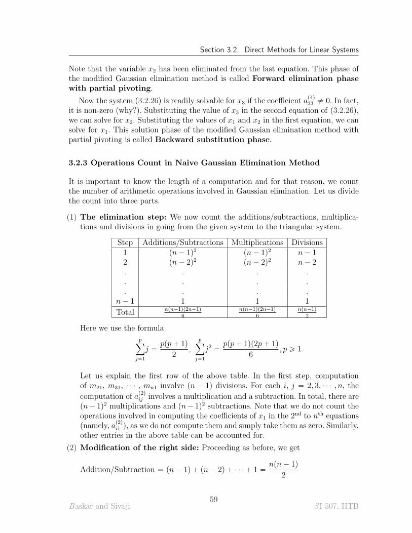
Section 3.2. Direct Methods for Linear Systems
Note that the variable x2 has been eliminated from the last equation. This phase ofthe modified Gaussian elimination method is called Forward elimination phasewith partial pivoting.
Now the system (3.2.26) is readily solvable for x3 if the coefficient ap4q
33 ‰ 0. In fact,it is non-zero (why?). Substituting the value of x3 in the second equation of (3.2.26),we can solve for x2. Substituting the values of x1 and x2 in the first equation, we cansolve for x1. This solution phase of the modified Gaussian elimination method withpartial pivoting is called Backward substitution phase.
3.2.3 Operations Count in Naive Gaussian Elimination Method
It is important to know the length of a computation and for that reason, we countthe number of arithmetic operations involved in Gaussian elimination. Let us dividethe count into three parts.
(1) The elimination step: We now count the additions/subtractions, multiplica-tions and divisions in going from the given system to the triangular system.
Step Additions/Subtractions Multiplications Divisions1 pn ´ 1q2 pn ´ 1q2 n ´ 12 pn ´ 2q2 pn ´ 2q2 n ´ 2. . . .. . . .. . . .
n ´ 1 1 1 1
Total npn´1qp2n´1q
6npn´1qp2n´1q
6npn´1q
2
Here we use the formula
pÿ
j“1
j “ppp ` 1q
2,
pÿ
j“1
j2 “ppp ` 1qp2p ` 1q
6, p ě 1.
Let us explain the first row of the above table. In the first step, computationof m21, m31, ¨ ¨ ¨ , mn1 involve pn ´ 1q divisions. For each i, j “ 2, 3, ¨ ¨ ¨ , n, the
computation of ap2q
ij involves a multiplication and a subtraction. In total, there arepn´ 1q2 multiplications and pn´ 1q2 subtractions. Note that we do not count theoperations involved in computing the coefficients of x1 in the 2nd to nth equations(namely, a
p2q
i1 ), as we do not compute them and simply take them as zero. Similarly,other entries in the above table can be accounted for.
(2) Modification of the right side: Proceeding as before, we get
Addition/Subtraction = pn ´ 1q ` pn ´ 2q ` ¨ ¨ ¨ ` 1 “npn ´ 1q
2
Baskar and Sivaji59
S I 507, IITB
Chapter 3. Numerical Linear Algebra
Multiplication/Division = pn ´ 1q ` pn ´ 2q ` ¨ ¨ ¨ ` 1 “npn ´ 1q
2
(3) The back substitution:
Addition/Subtraction = pn ´ 1q ` pn ´ 2q ` ¨ ¨ ¨ ` 1 “npn ´ 1q
2
Multiplication/Division = n ` pn ´ 1q ` ¨ ¨ ¨ ` 1 “npn ` 1q
2
Total number of operations: The total number of operations in obtaining x is
Addition/Subtraction =npn ´ 1qp2n ´ 1q
6+npn ´ 1q
2+npn ´ 1q
2=npn ´ 1qp2n ` 5q
6
Multiplication/Division =npn2 ` 3n ´ 1q
3Even if we take only multiplication and division into consideration, we see that
for large value of n, the operation count required for Gaussian elimination is about13n3. This means that as n doubled, the cost of solving the linear system goes up by a
factor of 8. In addition, most of the cost of Gaussian elimination is in the eliminationstep. For elimination, we have
Multiplication/Division =npn ´ 1qp2n ´ 1q
6`npn ´ 1q
2“n3
3
ˆ
1 ´1
n2
˙
«1
3n3.
The operation count in
Elimination step “ Opn3q,
RHS modification “ Opn2q,
Backward substitution “ Opn2q,
as n Ñ 8. Hence, once the elimination part is completed, it is much less expensiveto solve the linear system.
3.2.4 Thomas Method for Tri-diagonal System
The Gaussian elimination method can be simplified in the case of a tri-diagonalsystem so as to increase the efficiency. The resulting simplified method is called theThomas method.
A tri-diagonal system of linear equations is of the form
Baskar and Sivaji60
S I 507, IITB
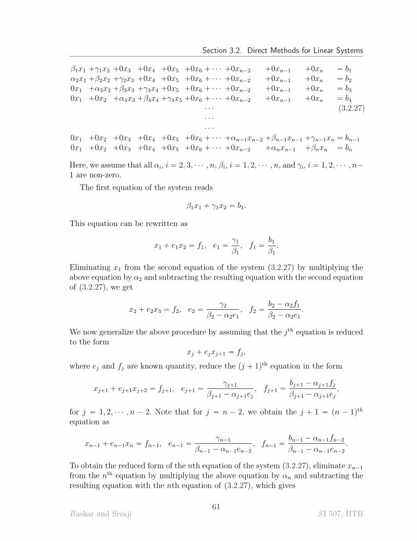
Section 3.2. Direct Methods for Linear Systems
β1x1 `γ1x2 `0x3 `0x4 `0x5 `0x6 ` ¨ ¨ ¨ `0xn´2 `0xn´1 `0xn “ b1α2x1 `β2x2 `γ2x3 `0x4 `0x5 `0x6 ` ¨ ¨ ¨ `0xn´2 `0xn´1 `0xn “ b20x1 `α3x2 `β3x3 `γ3x4 `0x5 `0x6 ` ¨ ¨ ¨ `0xn´2 `0xn´1 `0xn “ b30x1 `0x2 `α4x3 `β4x4 `γ4x5 `0x6 ` ¨ ¨ ¨ `0xn´2 `0xn´1 `0xn “ b4
¨ ¨ ¨
¨ ¨ ¨
¨ ¨ ¨
0x1 `0x2 `0x3 `0x4 `0x5 `0x6 ` ¨ ¨ ¨ `αn´1xn´2 `βn´1xn´1 `γn´1xn “ bn´1
0x1 `0x2 `0x3 `0x4 `0x5 `0x6 ` ¨ ¨ ¨ `0xn´2 `αnxn´1 `βnxn “ bn
(3.2.27)
Here, we assume that all αi, i “ 2, 3, ¨ ¨ ¨ , n, βi, i “ 1, 2, ¨ ¨ ¨ , n, and γi, i “ 1, 2, ¨ ¨ ¨ , n´
1 are non-zero.
The first equation of the system reads
β1x1 ` γ1x2 “ b1.
This equation can be rewritten as
x1 ` e1x2 “ f1, e1 “γ1β1, f1 “
b1β1.
Eliminating x1 from the second equation of the system (3.2.27) by multiplying theabove equation by α2 and subtracting the resulting equation with the second equationof (3.2.27), we get
x2 ` e2x3 “ f2, e2 “γ2
β2 ´ α2e1, f2 “
b2 ´ α2f1β2 ´ α2e1
.
We now generalize the above procedure by assuming that the jth equation is reducedto the form
xj ` ejxj`1 “ fj,
where ej and fj are known quantity, reduce the pj ` 1qth equation in the form
xj`1 ` ej`1xj`2 “ fj`1, ej`1 “γj`1
βj`1 ´ αj`1ej, fj`1 “
bj`1 ´ αj`1fjβj`1 ´ αj`1ej
,
for j “ 1, 2, ¨ ¨ ¨ , n ´ 2. Note that for j “ n ´ 2, we obtain the j ` 1 “ pn ´ 1qth
equation as
xn´1 ` en´1xn “ fn´1, en´1 “γn´1
βn´1 ´ αn´1en´2
, fn´1 “bn´1 ´ αn´1fn´2
βn´1 ´ αn´1en´2
.
To obtain the reduced form of the nth equation of the system (3.2.27), eliminate xn´1
from the nth equation by multiplying the above equation by αn and subtracting theresulting equation with the nth equation of (3.2.27), which gives
Baskar and Sivaji61
S I 507, IITB
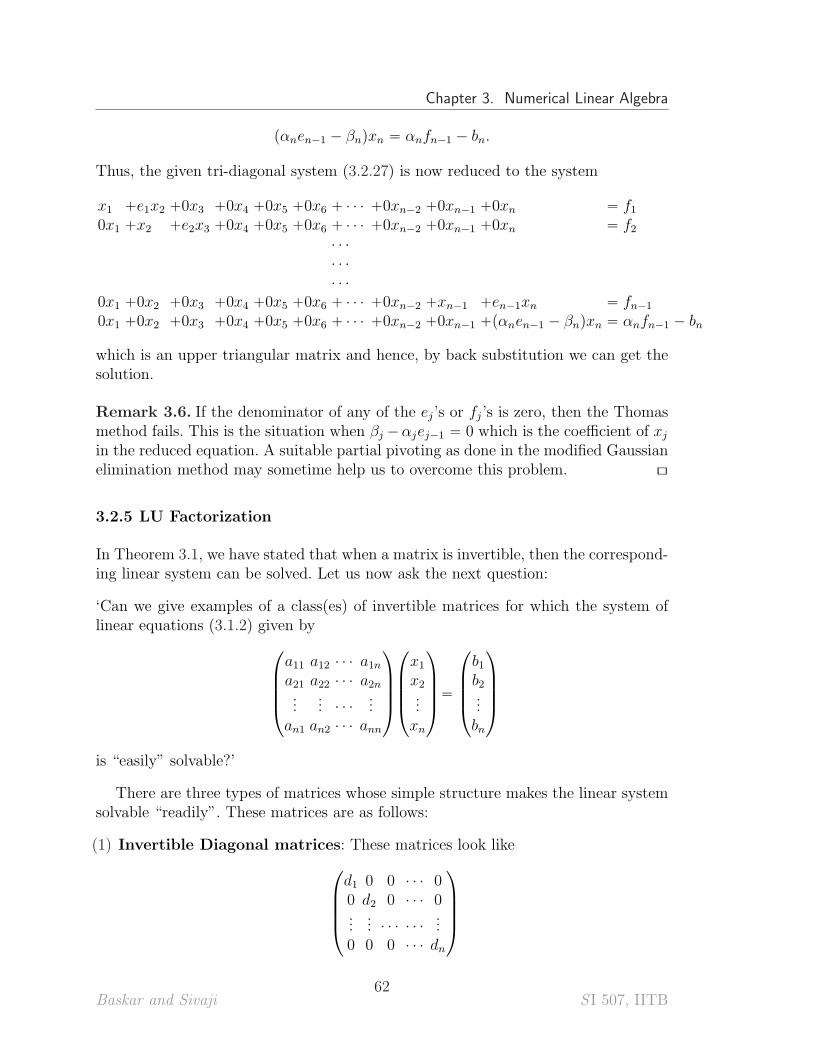
Chapter 3. Numerical Linear Algebra
pαnen´1 ´ βnqxn “ αnfn´1 ´ bn.
Thus, the given tri-diagonal system (3.2.27) is now reduced to the system
x1 `e1x2 `0x3 `0x4 `0x5 `0x6 ` ¨ ¨ ¨ `0xn´2 `0xn´1 `0xn “ f10x1 `x2 `e2x3 `0x4 `0x5 `0x6 ` ¨ ¨ ¨ `0xn´2 `0xn´1 `0xn “ f2
¨ ¨ ¨
¨ ¨ ¨
¨ ¨ ¨
0x1 `0x2 `0x3 `0x4 `0x5 `0x6 ` ¨ ¨ ¨ `0xn´2 `xn´1 `en´1xn “ fn´1
0x1 `0x2 `0x3 `0x4 `0x5 `0x6 ` ¨ ¨ ¨ `0xn´2 `0xn´1 `pαnen´1 ´ βnqxn “ αnfn´1 ´ bn
which is an upper triangular matrix and hence, by back substitution we can get thesolution.
Remark 3.6. If the denominator of any of the ej’s or fj’s is zero, then the Thomasmethod fails. This is the situation when βj ´αjej´1 “ 0 which is the coefficient of xjin the reduced equation. A suitable partial pivoting as done in the modified Gaussianelimination method may sometime help us to overcome this problem. [\
3.2.5 LU Factorization
In Theorem 3.1, we have stated that when a matrix is invertible, then the correspond-ing linear system can be solved. Let us now ask the next question:
‘Can we give examples of a class(es) of invertible matrices for which the system oflinear equations (3.1.2) given by
¨
˚
˚
˚
˝
a11 a12 ¨ ¨ ¨ a1na21 a22 ¨ ¨ ¨ a2n...
... ¨ ¨ ¨...
an1 an2 ¨ ¨ ¨ ann
˛
‹
‹
‹
‚
¨
˚
˚
˚
˝
x1x2...xn
˛
‹
‹
‹
‚
“
¨
˚
˚
˚
˝
b1b2...bn
˛
‹
‹
‹
‚
is “easily” solvable?’
There are three types of matrices whose simple structure makes the linear systemsolvable “readily”. These matrices are as follows:
(1) Invertible Diagonal matrices: These matrices look like
¨
˚
˚
˚
˝
d1 0 0 ¨ ¨ ¨ 00 d2 0 ¨ ¨ ¨ 0...
... ¨ ¨ ¨ ¨ ¨ ¨...
0 0 0 ¨ ¨ ¨ dn
˛
‹
‹
‹
‚
Baskar and Sivaji62
S I 507, IITB
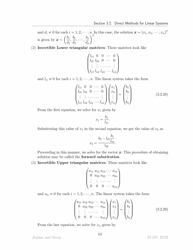
Section 3.2. Direct Methods for Linear Systems
and di ‰ 0 for each i “ 1, 2, ¨ ¨ ¨ , n. In this case, the solution x “ px1, x2, ¨ ¨ ¨ , xnqT
is given by x “
ˆ
b1d1,b2d2, ¨ ¨ ¨ ,
bndn
˙T
.
(2) Invertible Lower triangular matrices: These matrices look like¨
˚
˚
˚
˝
l11 0 0 ¨ ¨ ¨ 0l21 l22 0 ¨ ¨ ¨ 0...
... ¨ ¨ ¨ ¨ ¨ ¨...
ln1 ln2 ln3 ¨ ¨ ¨ lnn
˛
‹
‹
‹
‚
and lii ‰ 0 for each i “ 1, 2, ¨ ¨ ¨ , n. The linear system takes the form¨
˚
˚
˚
˝
l11 0 0 ¨ ¨ ¨ 0l21 l22 0 ¨ ¨ ¨ 0...
... ¨ ¨ ¨ ¨ ¨ ¨...
ln1 ln2 ln3 ¨ ¨ ¨ lnn
˛
‹
‹
‹
‚
¨
˚
˚
˚
˝
x1x2...xn
˛
‹
‹
‹
‚
“
¨
˚
˚
˚
˝
b1b2...bn
˛
‹
‹
‹
‚
(3.2.28)
From the first equation, we solve for x1 given by
x1 “b1l11.
Substituting this value of x1 in the second equation, we get the value of x2 as
x2 “
b2 ´ l21b1l11
l22.
Proceeding in this manner, we solve for the vector x. This procedure of obtainingsolution may be called the forward substitution.
(3) Invertible Upper triangular matrices: These matrices look like¨
˚
˚
˚
˝
u11 u12 u13 ¨ ¨ ¨ u1n0 u22 u23 ¨ ¨ ¨ u2n...
... ¨ ¨ ¨ ¨ ¨ ¨...
0 0 0 ¨ ¨ ¨ unn
˛
‹
‹
‹
‚
and uii ‰ 0 for each i “ 1, 2, ¨ ¨ ¨ , n. The linear system takes the form¨
˚
˚
˚
˝
u11 u12 u13 ¨ ¨ ¨ u1n0 u22 u23 ¨ ¨ ¨ u2n...
... ¨ ¨ ¨ ¨ ¨ ¨...
0 0 0 ¨ ¨ ¨ unn
˛
‹
‹
‹
‚
¨
˚
˚
˚
˝
x1x2...xn
˛
‹
‹
‹
‚
“
¨
˚
˚
˚
˝
b1b2...bn
˛
‹
‹
‹
‚
(3.2.29)
From the last equation, we solve for xn given by
Baskar and Sivaji63
S I 507, IITB
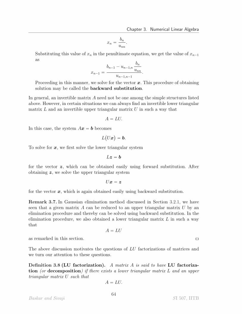
Chapter 3. Numerical Linear Algebra
xn “bnunn
.
Substituting this value of xn in the penultimate equation, we get the value of xn´1
as
xn´1 “
bn´1 ´ un´1,nbnunn
un´1,n´1
.
Proceeding in this manner, we solve for the vector x. This procedure of obtainingsolution may be called the backward substitution.
In general, an invertible matrix A need not be one among the simple structures listedabove. However, in certain situations we can always find an invertible lower triangularmatrix L and an invertible upper triangular matrix U in such a way that
A “ LU.
In this case, the system Ax “ b becomes
L`
Ux˘
“ b.
To solve for x, we first solve the lower triangular system
Lz “ b
for the vector z, which can be obtained easily using forward substitution. Afterobtaining z, we solve the upper triangular system
Ux “ z
for the vector x, which is again obtained easily using backward substitution.
Remark 3.7. In Gaussian elimination method discussed in Section 3.2.1, we haveseen that a given matrix A can be reduced to an upper triangular matrix U by anelimination procedure and thereby can be solved using backward substitution. In theelimination procedure, we also obtained a lower triangular matrix L in such a waythat
A “ LU
as remarked in this section. [\
The above discussion motivates the questions of LU factorizations of matrices andwe turn our attention to these questions.
Definition 3.8 (LU factorization). A matrix A is said to have LU factoriza-tion (or decomposition) if there exists a lower triangular matrix L and an uppertriangular matrix U such that
A “ LU.
Baskar and Sivaji64
S I 507, IITB
Section 3.2. Direct Methods for Linear Systems
Clearly if a matrix has an LU decomposition, the matrices L and U are not uniqueas
A “ LU “ pLDqpD´1Uq “ LU
for any invertible diagonal matrix D. Note that A “ LU is also an LU decompositionof A as L is a lower triangular matrix and U is an upper triangular matrix.
There are three special LU decompositions that we will discuss now.
Doolittle’s factorization
Definition 3.9 (Doolittle’s factorization). A matrix A is said to have a Doolit-tle’s factorization if there exists a lower triangular matrix L with all diagonal elementsas 1, and an upper triangular matrix U such that
A “ LU.
We now state the sufficient condition under which the Doolittle’s factorization of agiven matrix exists. For this, we need the notion of leading principal minors of a givenmatrix, which we define first and then state the required theorem.
Definition 3.10 (Principal Minors of a Matrix).
(1) Let A be an n ˆ n matrix. A sub-matrix of order k (ă n) of the matrix A is ak ˆ k matrix obtained by removing n ´ k rows and n ´ k columns from A.
The determinant of such a sub-matrix of order k of A is called a minor of orderk of the matrix A.
(2) The principal sub-matrix of order k of the matrix A is obtained by removingthe last n ´ k rows and the last n ´ k columns from A.
The determinant of the leading principal sub-matrix of order k of A is called theprincipal minor of order k of the matrix A.
(3) A principal sub-matrix and the corresponding principal minor are called the lead-ing principal sub-matrix and the leading principal minor of order k, re-spectively, if k ă n.
Example 3.11. Consider the 3 ˆ 3 matrix
A “
¨
˝
a11 a12 a13a21 a22 a23a31 a32 a33
˛
‚.
There are two leading principal minors corresponding to the matrix A.
• The leading principal minor of order 1 of A is
|a11| “ a11.
Baskar and Sivaji65
S I 507, IITB
Chapter 3. Numerical Linear Algebra
• The leading principal minor of order 2 of A is
ˇ
ˇ
ˇ
ˇ
a11 a12a21 a22
ˇ
ˇ
ˇ
ˇ
“ a11a22 ´ a12a21.
Theorem 3.12. Let n ě 2, and A be an n ˆ n matrix such that all of its first n ´ 1leading principal minors are non-zero. Then A has an LU-decomposition where L isa unit lower triangular matrix and U is an upper triangular matrix. That is, A hasa Doolittle’s factorization.
Proof: Let P pnq denote the following statement.
“P pnq: Every n ˆ n matrix all of whose first n ´ 1 leading principal minors arenon-zero has a Doolittle’s factorization.”
We want to prove that the statement P pnq is true for all natural numbers that aregreater than or equal to 2, using mathematical induction.
Step 1: (P p2q is true) Let A “
ˆ
a11 a12a21 a22
˙
be a 2 ˆ 2 matrix such that its leading
principal minor is non-zero. We want to prove that A has a Doolittle’s factorizationA “ LU where
L “
ˆ
1 0l21 1
˙
, U “
ˆ
u11 u120 u22
˙
The equality A “ LU now becomes
ˆ
a11 a12a21 a22
˙
“
ˆ
u11 u12l21u11 l21u12 ` u22
˙
(3.2.30)
Equating the elements of the first rows of the two matrices in the equation (3.2.30),we get
a11 “ u11, a12 “ u12.
That is, the first row of U has been found. Now equating the elements of the secondrows of the two matrices in the equation (3.2.30), we get
a21 “ l21u11, a22 “ l21u12 ` u22.
From the last equation, in view of a11 ‰ 0 (as it is the leading principal minor of A),we get
l21 “a21u11
“a21a11
, u22 “ a22 “ l21u12 “ a22 “a21a11
a12.
Thus the statement P p2q is true.
Step 2: Assume that P pkq is true. We will prove that P pk`1q is true. Let us assumethat A is an pk ` 1q ˆ pk ` 1q matrix such that its first k leading principal minorsare non-zero. Let Ak denote the leading sub-matrix consisting of the first k rows and
Baskar and Sivaji66
S I 507, IITB
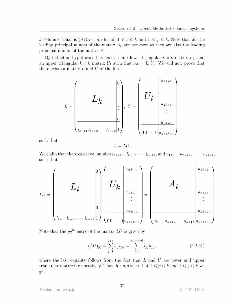
Section 3.2. Direct Methods for Linear Systems
k columns. That is pAkqij “ aij for all 1 ď i ď k and 1 ď j ď k. Note that all theleading principal minors of the matrix Ak are non-zero as they are also the leadingprincipal minors of the matrix A.
By induction hypothesis there exist a unit lower triangular k ˆ k matrix Lk, andan upper triangular k ˆ k matrix Uk such that Ak “ LkUk. We will now prove thatthere exists a matrix L and U of the form
L “
¨
˚
˚
˚
˚
˚
˚
˚
˚
˚
˚
˚
˚
˚
˝
Lk
0
...
0
lk`1 1 lk`1 2 ¨ ¨ ¨ lk`1 k 1
˛
‹
‹
‹
‹
‹
‹
‹
‹
‹
‹
‹
‹
‹
‚
, U “
¨
˚
˚
˚
˚
˚
˚
˚
˚
˚
˚
˚
˚
˚
˚
˚
˝
Uk
u1 k`1
u2 k`1...
uk k`1
0 0 ¨ ¨ ¨ 0 uk`1 k`1
˛
‹
‹
‹
‹
‹
‹
‹
‹
‹
‹
‹
‹
‹
‹
‹
‚
.
such thatA “ LU.
We claim that there exist real numbers lk`1 1, lk`1 2, ¨ ¨ ¨ lk`1 k, and u1 k`1, u2 k`1, ¨ ¨ ¨ , uk`1 k`1
such that
LU “
¨
˚
˚
˚
˚
˚
˚
˚
˚
˚
˚
˚
˚
˚
˝
Lk
0
...
0
lk`1 1 lk`1 2 ¨ ¨ ¨ lk`1 k 1
˛
‹
‹
‹
‹
‹
‹
‹
‹
‹
‹
‹
‹
‹
‚
¨
˚
˚
˚
˚
˚
˚
˚
˚
˚
˚
˚
˚
˚
˚
˚
˝
Uk
u1 k`1
u2 k`1...
uk k`1
0 0 ¨ ¨ ¨ 0 uk`1 k`1
˛
‹
‹
‹
‹
‹
‹
‹
‹
‹
‹
‹
‹
‹
‹
‹
‚
“
¨
˚
˚
˚
˚
˚
˚
˚
˚
˚
˚
˚
˚
˚
˚
˚
˝
Ak
a1 k`1
a2 k`1...
ak k`1
ak`1 1 ak`1 2 ¨ ¨ ¨ ak`1 k ak`1 k`1
˛
‹
‹
‹
‹
‹
‹
‹
‹
‹
‹
‹
‹
‹
‹
‹
‚
.
Note that the pqth entry of the matrix LU is given by
pLUqpq “
k`1ÿ
j“1
lpjujq “
mintp,quÿ
j“1
lpjujq, (3.2.31)
where the last equality follows from the fact that L and U are lower and uppertriangular matrices respectively. Thus, for p, q such that 1 ď p ď k and 1 ď q ď k weget
Baskar and Sivaji67
S I 507, IITB
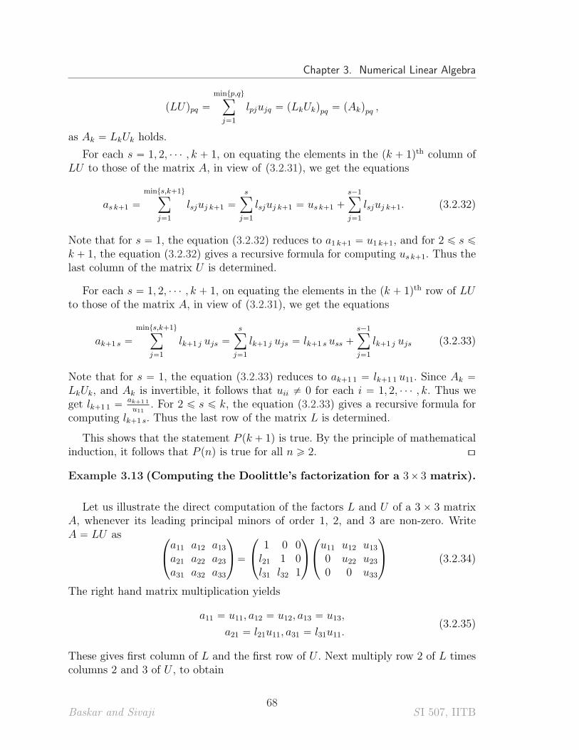
Chapter 3. Numerical Linear Algebra
pLUqpq “
mintp,quÿ
j“1
lpjujq “ pLkUkqpq “ pAkqpq ,
as Ak “ LkUk holds.
For each s “ 1, 2, ¨ ¨ ¨ , k ` 1, on equating the elements in the pk ` 1qth column ofLU to those of the matrix A, in view of (3.2.31), we get the equations
as k`1 “
mints,k`1uÿ
j“1
lsjuj k`1 “
sÿ
j“1
lsjuj k`1 “ us k`1 `
s´1ÿ
j“1
lsjuj k`1. (3.2.32)
Note that for s “ 1, the equation (3.2.32) reduces to a1 k`1 “ u1 k`1, and for 2 ď s ď
k ` 1, the equation (3.2.32) gives a recursive formula for computing us k`1. Thus thelast column of the matrix U is determined.
For each s “ 1, 2, ¨ ¨ ¨ , k ` 1, on equating the elements in the pk ` 1qth row of LUto those of the matrix A, in view of (3.2.31), we get the equations
ak`1 s “
mints,k`1uÿ
j“1
lk`1 j ujs “
sÿ
j“1
lk`1 j ujs “ lk`1 s uss `
s´1ÿ
j“1
lk`1 j ujs (3.2.33)
Note that for s “ 1, the equation (3.2.33) reduces to ak`1 1 “ lk`1 1 u11. Since Ak “
LkUk, and Ak is invertible, it follows that uii ‰ 0 for each i “ 1, 2, ¨ ¨ ¨ , k. Thus weget lk`1 1 “
ak`1 1
u11. For 2 ď s ď k, the equation (3.2.33) gives a recursive formula for
computing lk`1 s. Thus the last row of the matrix L is determined.
This shows that the statement P pk ` 1q is true. By the principle of mathematicalinduction, it follows that P pnq is true for all n ě 2. [\
Example 3.13 (Computing the Doolittle’s factorization for a 3ˆ 3 matrix).
Let us illustrate the direct computation of the factors L and U of a 3 ˆ 3 matrixA, whenever its leading principal minors of order 1, 2, and 3 are non-zero. WriteA “ LU as
¨
˝
a11 a12 a13a21 a22 a23a31 a32 a33
˛
‚“
¨
˝
1 0 0l21 1 0l31 l32 1
˛
‚
¨
˝
u11 u12 u130 u22 u230 0 u33
˛
‚ (3.2.34)
The right hand matrix multiplication yields
a11 “ u11, a12 “ u12, a13 “ u13,
a21 “ l21u11, a31 “ l31u11.(3.2.35)
These gives first column of L and the first row of U . Next multiply row 2 of L timescolumns 2 and 3 of U , to obtain
Baskar and Sivaji68
S I 507, IITB
Section 3.2. Direct Methods for Linear Systems
a22 “ l21u12 ` u22, a23 “ l21u13 ` u23. (3.2.36)
These can be solved for u22 and u23. Next multiply row 3 of L to obtain
l31u12 ` l32u22 “ a32, l31u13 ` l32u23 ` u33 “ a33. (3.2.37)
These equations yield values for l32 and u33, completing the construction of L and U .In this process, we must have u11 ‰ 0, u22 ‰ 0 in order to solve for L, which is truebecause of the assumptions that all the leading principal minors of A are non-zero.
The decomposition we have found is the Doolittle’s factorization of A. [\
Example 3.14. Consider the matrix
A “
¨
˝
1 1 ´11 2 ´2
´2 1 1
˛
‚.
Using (3.2.35), we get
u11 “ 1, u12 “ 1, u13 “ ´1, l21 “a21u11
“ 1, l31 “a31u11
“ ´2
Using (3.2.36) and (3.2.37),
u22 “ a22 ´ l21u12 “ 2 ´ 1 ˆ 1 “ 1
u23 “ a23 ´ l21u13 “ ´2 ´ 1 ˆ p´1q “ ´1
l32 “ pa32 ´ l31u12q{u22 “ p1 ´ p´2q ˆ 1q{1 “ 3
u33 “ a33 ´ l31u13 ´ l32u23 “ 1 ´ p´2q ˆ p´1q ´ 3 ˆ p´1q “ 2
Thus we obtain the Doolittle’s factorization of A as
A “
¨
˝
1 0 01 1 0
´2 3 1
˛
‚
¨
˝
1 1 ´10 1 ´10 0 2
˛
‚
Further, taking b “ p1, 1, 1qT , we now solve the system Ax “ b using LU factorization,with the matrix A given above. As discussed earlier, first we have to solve the lowertriangular system
¨
˝
1 0 01 1 0
´2 3 1
˛
‚
¨
˝
z1z2z3
˛
‚“
¨
˝
111
˛
‚.
Forward substitution yields z1 “ 1, z2 “ 0, z3 “ 3. Keeping the vector z “ p1, 0, 3qT
as the right hand side, we now solve the upper triangular system¨
˝
1 1 ´10 1 ´10 0 2
˛
‚
¨
˝
x1x2x3
˛
‚“
¨
˝
103
˛
‚.
Backward substitution yields x1 “ 1, x2 “ 3{2, x3 “ 3{2. [\
Baskar and Sivaji69
S I 507, IITB
Chapter 3. Numerical Linear Algebra
Crout’s factorization
In Doolittle’s factorization, the lower triangular matrix has special property. If weask the upper triangular matrix to have special property in the LU decomposition,it is known as Crout’s factorization. We give the definition below.
Definition 3.15 (Crout’s factorization). A matrix A is said to have a Crout’sfactorization if there exists a lower triangular matrix L, and an upper triangularmatrix U with all diagonal elements as 1 such that
A “ LU.
The computation of the Crout’s factorization for a 3 ˆ 3 matrix can be done ina similar way as done for Doolittle’s factorization in Example 3.13. For invertiblematrices, one can easily obtain Doolittle’s factorization from Crout’s factorizationand vice versa. See the Example ?? below.
Cholesky’s factorization
Before we introduce Cholesky’s factorization, we recall the concept of a positivedefinite matrix.
Definition 3.16 (Positive Definite Matrix).
A symmetric matrix A is said to be positive definite if
xTAx ą 0,
for every non-zero vector x.
We state below some useful results concerning positive definite matrices.
Lemma 3.17. The following statements concerning a symmetric nˆn matrix A areequivalent.
(1) The matrix A is positive definite.
(2) All the principal minors of the matrix A are positive.
(3) All the eigenvalues of the matrix A are positive.
Proof: The statements (1) and (2) are equivalent by definition. The proof of equiv-alence of (3) with other two statements is out of the scope of this course. [\
We now define Cholesky’s factorization.
Definition 3.18 (Cholesky’s factorization). A matrix A is said to have aCholesky’s factorization if there exists a lower triangular matrix L such that
A “ LLT .
Baskar and Sivaji70
S I 507, IITB
Section 3.2. Direct Methods for Linear Systems
Remark 3.19. It is clear from the definition that if a matrix has a Cholesky’s fac-torization, then the matrix have to be necessarily a symmetric matrix. [\
Theorem 3.20. If A is an nˆn symmetric and positive definite matrix, then A hasa unique factorization
A “ LLT
where L is a lower triangular matrix with positive diagonal elements.
Proof: We prove the theorem by induction. The proof of the theorem is trivial whenn “ 1. Let us assume that the theorem holds for n “ k for some k P N. That is, weassume that for every k ˆ k symmetric and positive definite matrix Bk, there existsa unique lower triangular k ˆ k matrix Lk such that
Bk “ LkLTk .
We prove the theorem for n “ k` 1. Let A be a pk` 1q ˆ pk` 1q symmetric positivedefinite matrix.
We first observe that the matrix A can be written as
A “
ˆ
Ak aaT apk`1qpk`1q
˙
,
where Ak is the kˆk principal sub-matrix of A and a “ pa1pk`1q, a2pk`1q, ¨ ¨ ¨ , akpk`1qqT .
Observe that Ak is positive definite and therefore by our assumption, there exists aunique k ˆ k lower triangular matrix Lk such that Ak “ LkL
Tk . Define
L “
ˆ
Lk 0lT lpk`1qpk`1q
˙
,
where the real number lpk`1qpk`1q and the vector l “ pl1pk`1q, l2pk`1q, ¨ ¨ ¨ , lkpk`1qqT are
to be chosen such that A “ LLT . That isˆ
Ak aaT apk`1qpk`1q
˙
“
ˆ
Lk 0lT lpk`1qpk`1q
˙ˆ
LTk l
0T lpk`1qpk`1q
˙
. (3.2.38)
Here 0 denotes the zero vector of dimension k. Clearly,
Lkl “ a, (3.2.39)
which by forward substitution yields the vector l. Here, we need to justify that Lk isinvertible, which is left as an exercise.
Finally, we have lT l ` l2pk`1qpk`1q “ apk`1qpk`1q and this gives
l2pk`1qpk`1q “ apk`1qpk`1q ´ lT l, (3.2.40)
provided the positivity of l2pk`1qpk`1q is justified, which follows from taking determinant
on both sides of (3.2.38) and using the property (3) of Lemma 3.17. A complete proofof this justification is left as an exercise. [\
Baskar and Sivaji71
S I 507, IITB
Chapter 3. Numerical Linear Algebra
Example 3.21. Consider the matrix
A “
¨
˝
9 3 ´23 2 3
´2 3 23
˛
‚.
We can check that this matrix is positive definite by any of the equivalent conditionslisted in Lemma 3.17. Therefore, we expect a unique Cholesky’s factorization for A.
(1) For n “ 1, we have A1 “ p9q and therefore let us take L1 “ p3q.
(2) For n “ 2, we have
A2 “
ˆ
9 33 2
˙
.
Therefore,
L2 “
ˆ
L1 0l l22
˙
“
ˆ
3 0l l22
˙
.
This gives l “ 1 and l2 ` l222 “ 2 or l22 “ 1. Thus, we have
L2 “
ˆ
3 01 1
˙
.
(3) For n “ 3, we take
L “
ˆ
L2 0lT l33
˙
,
where lT “ pl13, l23q and l33 are to be obtained in such a way that A “ LLT .The vector l is obtained by solving the lower triangular system (3.2.39) witha “ p´2, 3qT (by forward substitution), which gives l “ p´2{3, 11{3qT . Finally,from (3.2.40), we have l233 “ 82{9. Thus, the required lower triangular matrix L is
L “
¨
˝
3 0 01 1 0
´2{3 11{3?82{3
˛
‚.
It is straightforward to check that A “ LLT . [\
It can be observed that the idea of LU factorization method for solving a system oflinear equations is parallel to the idea of Gaussian elimination method. However, LUfactorization method has an advantage that once the factorization A “ LU is done,the solution of the linear system Ax “ b is reduced to solving two triangular systems.Thus, if we want to solve a large set of linear systems where the coefficient matrix Ais fixed but the right hand side vector b varies, we can do the factorization once forA and then use this factorization with different b vectors. This is obviously going toreduce the computation cost drastically as we have seen in the operation counting ofGaussian elimination method that the elimination part is the most expensive part ofthe computation.
Baskar and Sivaji72
S I 507, IITB
Section 3.3. Matrix Norms and Condition Number of a Matrix
3.3 Matrix Norms and Condition Number of a Matrix
Given any two real numbers α and β, the distance between them may be taken tobe |α ´ β|. We can also compare their magnitudes |α| and |β|. Vector Norm may bethought of as a generalization of the Modulus | ¨ | concept to deal with vectors andin general matrices.
Definition 3.22 (Vector Norm).
A vector norm on Rn is a function } ¨ } : Rn Ñ r0,8q having the followingproperties:
(1) }x} ě 0 for all x P Rn.
(2) }x} “ 0 if and only if x “ 0.
(3) }αx} “ |α|}x} for all x P Rn and for all α P R.(4) }x ` y} ď }x} ` }y} for all x,y P Rn.
The condition 4 in the above definition is called the triangle inequality.
We use the following notation for a vector x P Rn in terms of its components:
x “ px1, x2, ¨ ¨ ¨ , xnqT .
Example 3.23. There can be many vector norms on Rn. We will describe threeimportant vector norms defined on Rn now.
(1) Euclidean Norm on Rn is denoted by } ¨ }2, and is defined by
}x}2 “
d
nÿ
i“1
|xi|2. (3.3.41)
(2) l8 norm, which is also called maximum norm, on Rn is denoted by } ¨ }8, andis defined by
}x}8 “ max t |x1|, |x2|, ¨ ¨ ¨ , |xn| u . (3.3.42)
(3) l1 norm on Rn is denoted by } ¨ }1, and is defined by
}x}1 “ |x1| ` |x2| ` ¨ ¨ ¨ ` |xn|. (3.3.43)
All the three norms defined above are indeed norms; it is easy to verify that theysatisfy the defining conditions of a norm given in Definition 3.22. [\
Example 3.24. Let us compute norms of some vectors now. Let x “ p4, 4,´4, 4qT ,y “ p0, 5, 5, 5qT , z “ p6, 0, 0, 0qT . Verify that }x}1 “ 16, }y}1 “ 15, }z}1 “ 6;}x}2 “ 8, }y}2 “ 8.66, }z}2 “ 6; }x}8 “ 4, }y}8 “ 5, }z}8 “ 6.
Baskar and Sivaji73
S I 507, IITB
Chapter 3. Numerical Linear Algebra
From this example we see that asking which vector is big does not make sense.But once the norm is fixed, this question makes sense as the answer depends on thenorm used. In this example each vector is big compared to other two but in differentnorms. [\
Remark 3.25. In our computations, we employ any one of the norms depending onconvenience. It is a fact that “all vector norms on Rn are equivalent”; we will notelaborate further on this. [\
We can also define matrix norms on n ˆ n matrices, which helps us in findingdistance between two matrices.
Definition 3.26 (Matrix Norm).
A matrix norm on the vector space of all nˆn real matrices MnpRq is a function} ¨ } : MnpRq Ñ r0,8q having the following properties:
(1) }A} ě 0 for all A P MnpRq.
(2) }A} “ 0 if and only if A “ 0.
(3) }αA} “ |α|}A} for all A P MnpRq and for all α P R.(4) }A ` B} ď }A} ` }B} for all A,B P MnpRq.
As in the case of vector norms, the condition 4 in the above definition is called thetriangle inequality. For a matrix A P MnpRq, we use the notation
A “ paijq1ďiďn, 1ďjďn
where aij denotes the element in the ith row and jth column of A.
There can be many matrix norms on MnpRq. We will describe some of them now.
Example 3.27. The following define norms on MnpRq.
(1) }A} “
g
f
f
e
nÿ
i“1
nÿ
j“1
|aij|2 .
(2) }A} “ max t |aij| : 1 ď i ď n, 1 ď j ď n u .
(3) }A} “řn
i“1
řnj“1 |aij|.
All the three norms defined above are indeed norms; it is easy to verify that theysatisfy the defining conditions of a matrix norm of Definition 3.26. [\
Among matrix norms, there are special ones that satisfy very useful and importantproperties. They are called Matrix norms subordinate to a vector norm. Asthe name suggests, to define them we need to fix a vector norm. We will give a precisedefinition now.
Baskar and Sivaji74
S I 507, IITB
Section 3.3. Matrix Norms and Condition Number of a Matrix
Definition 3.28 (Matrix Norm subordinate to a vector norm).
Let } ¨ } be a vector norm on Rn and let A P MnpRq. The matrix norm of Asubordinate to the vector norm } ¨ } is defined by
}A} :“ sup t}Ax} : x P Rn, }x} “ 1u . (3.3.44)
The formula (3.3.44) indeed defines a matrix norm on MnpRq. The proof of this factis beyond the scope of our course. In this course, by matrix norm, we always meana norm subordinate to some vector norm. An equivalent and more useful formula forthe matrix norm subordinate to a vector norm is given in the following lemma.
Lemma 3.29. For any A P MnpRq and a given vector norm } ¨ }, we have
}A} “ maxz‰0
}Az}
}z}. (3.3.45)
Proof: For any z ‰ 0, we have x “ z{||z|| as a unit vector. Hence
max||x||“1
||Ax|| “ max||z||‰0
›
›
›
›
A
ˆ
z
||z||
˙›
›
›
›
“ max||z||‰0
||Az||
||z||.
[\
The matrix norm subordinate to a vector norm has additional properties as statedin the following theorem whose proof is left as an exercise.
Theorem 3.30. Let } ¨ } be a matrix norm subordinate to a vector norm. Then
(1) }Ax} ď }A}}x} for all x P Rn.
(2) }I} “ 1 where I is the identity matrix.
(3) }AB} ď }A} }B} for all A,B P MnpRq. [\
We will now state a few results concerning matrix norms subordinate to some ofthe vector norms described in Example 3.23. We will not discuss their proofs.
Theorem 3.31 (Matrix norm subordinate to the maximum norm).
The matrix norm subordinate to the l8 norm (also called maximum norm givenin (3.3.42)) on Rn is denoted by }A}8 and is given by
}A}8 “ max1ďiďn
nÿ
j“1
|aij|. (3.3.46)
The norm }A}8 given by the formula (3.3.46) is called the maximum-of-row-sumsnorm of A. [\
Baskar and Sivaji75
S I 507, IITB
Chapter 3. Numerical Linear Algebra
Theorem 3.32 (Matrix Norm Subordinate to the l1-norm).
The matrix norm subordinate to the l1 norm (given in (3.3.43)) on Rn is denotedby }A}1 and is given by
}A}1 “ max1ďjďn
nÿ
i“1
|aij|. (3.3.47)
The norm }A}1 given by the formula (3.3.47) is called the maximum-of-column-sums norm of A. [\
Description and computation of the matrix norm subordinate to the Euclidean vectornorm on Rn is more subtle.
Theorem 3.33 (Matrix norm subordinate to the Euclidean norm).
The matrix norm subordinate to the l2 norm (also called Euclidean norm givenin (3.3.41)) on Rn is denoted by }A}2 and is given by
}A}2 “b
max1ďiďn
|λi|, (3.3.48)
where λ1, λ2, ¨ ¨ ¨ , λn are eigenvalues of the matrix ATA. The norm }A}2 given by theformula (3.3.48) is called the spectral norm of A. [\
Example 3.34. Let us now compute }A}8 and }A}2 for the matrix
¨
˝
1 1 ´11 2 ´2
´2 1 1
˛
‚.
(1) }A}8 “ 5 since
3ÿ
j“1
|a1j| “ |1| ` |1| ` | ´ 1| “ 3,
3ÿ
j“1
|a2j| “ |1| ` |2| ` | ´ 2| “ 5,
3ÿ
j“1
|a3j| “ | ´ 2| ` |1| ` |1| “ 4.
(2) }A}2 « 3.5934 as the eigenvalues of ATA are λ1 « 0.0616, λ2 « 5.0256 andλ3 « 12.9128. Hence }A}2 «
?12.9128 « 3.5934. [\
The following theorem motivates the condition number for an invertible matrix whichis similar to the condition number defined for a function in Section 2.5.1.
Baskar and Sivaji76
S I 507, IITB
Section 3.3. Matrix Norms and Condition Number of a Matrix
Theorem 3.35. Let A be an invertible nˆn matrix. Let x and x be the solutions ofthe systems
Ax “ b and Ax “ b,
respectively, where b and b are given vectors. Then
}x ´ x}
}x}ď }A} }A´1}
}b ´ b}
}b}(3.3.49)
for any fixed vector norm and the matrix norm subordinate to this vector norm.
Proof: Since A is invertible, we have x ´ x “ A´1´
b ´ b¯
. Taking norms on both
sides and using the fact that }Ax} ď }A}}x} (see Theorem 3.30) holds for everyx P Rn, we get
}x ´ x} ď }A´1}}b ´ b} (3.3.50)
The last inequality (3.3.50) estimates the error in the solution caused by error onthe right hand side vector of the linear system Ax “ b. The inequality (3.3.49) isconcerned with estimating the relative error in the solution in terms of the relativeerror in the right hand side vector b.
Since Ax “ b, we get }b} “ }Ax} ď }A}}x}. Therefore }x} ě}b}
}A}. Using this
inequality in (3.3.50), we get (3.3.49). [\
Remark 3.36.
(1) In the above theorem, it is important to note that a vector norm is fixed and thematrix norm used is subordinate to this fixed vector norm.
(2) The theorem holds no matter which vector norm is fixed as long as the matrixnorm subordinate to it is used.
(3) In fact, whenever we do analysis on linear systems, we always fix a vector normand then use matrix norm subordinate to it. [\
Notice that the constant appearing on the right hand side of the inequality (3.3.49)(which is }A} }A´1}) depends only on the matrix A (for a given vector norm). Thisnumber is called the condition number of the matrix A. Notice that this conditionnumber depends very much on the vector norm being used on Rn and the matrixnorm that is subordinate to the vector norm.
Definition 3.37 (Condition Number of a Matrix). Let A be an nˆn invertiblematrix. Let a matrix norm be given that is subordinate to a vector norm. Then thecondition number of the matrix A (denoted by κpAq) is defined as
κpAq :“ }A} }A´1}. (3.3.51)
Baskar and Sivaji77
S I 507, IITB
Chapter 3. Numerical Linear Algebra
Remark 3.38. From Theorem 3.35, it is clear that if the condition number is small,then the relative error in the solution will also be small whenever the relative errorin the right hand side vector is small. On the other hand, if the condition number islarge, then the relative error could be very large even though the relative error in theright hand side vector is small. We illustrate this in the following example. [\
Example 3.39. The linear system
5x1 ` 7x2 “ 0.7
7x1 ` 10x2 “ 1
has the solution x1 “ 0, x2 “ 0.1. Let us denote this by x “ p0, 0.1qT , and the righthand side vector by b “ p0.7, 1qT . The perturbed system
5x1 ` 7x2 “ 0.69
7x1 ` 10x2 “ 1.01
has the solution x1 “ ´0.17, x2 “ 0.22, which we denote by x “ p´0.17, 0.22qT ,and the right hand side vector by b “ p0.69, 1.01qT . The relative error between thesolutions of the above systems in the l8 vector norm is given by
}x ´ x}8
}x}8
“ 1.7,
which is too high compared to the relative error in the right hand side vector whichis given by
}b ´ b}8
}b}8
“ 0.01.
The condition number of the coefficient matrix of the system is 289. Therefore themagnification of the relative error is expected (see the inequality (3.3.49)). [\
Definition 3.40. A matrix with a large condition number is said to be ill condi-tioned. A matrix with a small condition number is said to be well conditioned.
Remark 3.41. An immediate question is that how large should the condition numberbe to declare that a matrix is ill-conditioned. This quantification is very difficult inpractical situations as it depends on how large the relative error in the right handside vector and also the tolerance level of the user. That is, how much error a usercan tolerate in the application for which the linear system is solved. For instance, infinance related applications, even 20% of error may be tolerable, whereas in computingthe path of a missile even a 0.2% error may lead to fatal disasters. [\
Discussion of condition numbers of matrices is incomplete without the mention of thefamous Hilbert matrix.
Baskar and Sivaji78
S I 507, IITB
Section 3.3. Matrix Norms and Condition Number of a Matrix
Example 3.42. The Hilbert matrix of order n is given by
Hn “
¨
˚
˚
˚
˚
˚
˚
˝
1 12
13
¨ ¨ ¨ 1n
12
13
14
¨ ¨ ¨ 1n`1
¨ ¨ ¨ ¨
¨ ¨ ¨ ¨
¨ ¨ ¨ ¨1n
1n`1
1n`1
¨ ¨ ¨ 12n´1
˛
‹
‹
‹
‹
‹
‹
‚
(3.3.52)
For n “ 4, we have
κpH4q “ }H4}8}H´14 }8 “
25
1213620 « 28000
which may be taken as an ill-conditioned matrix. In fact, as the value of n increases,the corresponding condition number of the Hilbert matrix also increases. [\
An interesting and important question is that what kind of matrices could have largecondition numbers. A partial answer is stated in the following theorem.
Theorem 3.43. Let A P MnpRq be non-singular. Then, for any singular nˆn matrixB, we have
1
κpAqď
}A ´ B}
}A}. (3.3.53)
Proof. We have
1
κpAq“
1
}A}}A´1}“
1
}A}
¨
˚
˚
˝
1
maxx‰0
}A´1x}
}x}
˛
‹
‹
‚
ď1
}A}
¨
˚
˚
˝
1
}A´1y}
}y}
˛
‹
‹
‚
where y ‰ 0 is arbitrary. Take y “ Az, for some arbitrary vector z. Then we get
1
κpAqď
1
}A}
ˆ
}Az}
}z}
˙
.
Let z ‰ 0 be such that Bz “ 0 (this is possible since B is singular), we get
1
κpAqď
}pA ´ Bqz}
}A}}z}
ď}pA ´ Bq}}z}
}A}}z}
“}A ´B}
}A},
and we are done. [\
Baskar and Sivaji79
S I 507, IITB
Chapter 3. Numerical Linear Algebra
From the above theorem it is apparent that if A is close to a singular matrix, thenthe reciprocal of the condition number will be near to zero, ie., κpAq itself will belarge. Let us illustrate this in the following example.
Example 3.44. Clearly the matrix
B “
ˆ
1 11 1
˙
is not invertible. For any ϵ ą 0, let
A “
ˆ
1 1 ` ϵ1 ´ ϵ 1
˙
.
As ϵ ą 0, A is invertible and we have
A´1 “ ϵ´2
ˆ
1 ´1 ´ ϵ´1 ` ϵ 1
˙
.
Let us use the l8 norm on Rn. Then }A}8 “ 2 ` ϵ and }A´1}8 “ ϵ´2p2 ` ϵq. Hence
κpAq “ }A}8}A´1}8
“
ˆ
2 ` ϵ
ϵ
˙2
ą4
ϵ2.
Thus, if ϵ ď 0.01, then κpAq ě 40, 000. As ϵ Ñ 0, the matrix A tends to approachthe matrix B and consequently, the above inequality says that the condition numberκpAq tends to 8.
Also, we can see that when we attempt to solve the system Ax “ b, then the aboveinequality implies that a small relative perturbation in the right hand side vector bcould be magnified by a factor of at least 40, 000 for the relative error in the solution.[\
3.4 Iterative Methods for Linear Systems
In Sections 3.2.1 and 3.2.5 we have discussed methods that obtain exact solution of alinear system Ax “ b in the absence of floating point errors (i.e., exact arithmetic isused). Such methods are called the direct methods. The solution of a linear systemcan also be obtained using iterative procedures. Such methods are called iterativemethods. There are many iterative procedures out of which Jacobi and Gauss-Seidel methods are the simplest ones. In this section we introduce these methodsand discuss their convergence.
Baskar and Sivaji80
S I 507, IITB
Section 3.4. Iterative Methods for Linear Systems
3.4.1 Jacobi Method
In section 3.2.5, we have seen that when a linear system Ax “ b is such that thecoefficient matrix A is a diagonal matrix, then this system can be solved very easily.We explore this idea to build a new method based on iterative procedure. For this,we first rewrite the matrix A as
A “ D ´ C,
where D,C P MnpRq are such that
D “
¨
˚
˚
˚
˝
a11 0 ¨ ¨ ¨ 00 a22 ¨ ¨ ¨ 0...
... ¨ ¨ ¨...
0 0 ¨ ¨ ¨ ann
˛
‹
‹
‹
‚
,
where aii, i “ 1, 2, ¨ ¨ ¨ , n are the diagonal elements of the matrix A. Then the givensystem of linear equations can be re-written as
Dx “ Cx ` b. (3.4.54)
If we assume that the right hand side vector is fully known to us, then the abovesystem can be solved very easily as D is a diagonal matrix. But obviously, the righthand side vector cannot be a known quantity because it involves the unknown vectorx. Rather, if we choose (arbitrarily) some specific value for x, say x “ xp0q, then theresulting system
Dx “ Cxp0q ` b
can be readily solved. Let us call the solution of this system as xp1q. That is,
Dxp1q “ Cxp0q ` b.
Now taking x “ xp1q on the right hand side of (3.4.54) we can obtain the solutionof this system, which we denote as xp2q and repeat this procedure to get a generaliterative procedure as
Dxpk`1q “ Cxpkq ` b, k “ 0, 1, 2, ¨ ¨ ¨ .
If D is invertible, then the above iterative procedure can be written as
xpk`1q “ Bxpkq ` c, k “ 0, 1, 2, ¨ ¨ ¨ , (3.4.55)
where B “ D´1C and c “ D´1b. The iterative procedure (3.4.55) is called the Jacobimethod.
Baskar and Sivaji81
S I 507, IITB
Chapter 3. Numerical Linear Algebra
Example 3.45. Let us illustrate the Jacobi method in the case of 3 ˆ 3 system
a11x1 ` a12x2 ` a13x3 “ b1
a21x1 ` a22x2 ` a23x3 “ b2
a31x1 ` a32x2 ` a33x3 “ b3,
where a11 ‰ 0, a22 ‰ 0, and a33 ‰ 0. We can rewrite the above system of linearequations as
x1 “1
a11pb1 ´ a12x2 ´ a13x3q
x2 “1
a22pb2 ´ a21x1 ´ a23x3q
x3 “1
a33pb3 ´ a31x1 ´ a32x2q
Let xp0q “ pxp0q
1 , xp0q
2 , xp0q
3 qT be an initial guess to the true solution x, which is chosenarbitrarily. Define a sequence of iterates (for k “ 0, 1, 2, ¨ ¨ ¨ ) by
xpk`1q
1 “1
a11pb1 ´ a12x
pkq
2 ´ a13xpkq
3 q
xpk`1q
2 “1
a22pb2 ´ a21x
pkq
1 ´ a23xpkq
3 q
xpk`1q
3 “1
a33pb3 ´ a31x
pkq
1 ´ a32xpkq
2 q.
,
/
/
/
/
/
/
.
/
/
/
/
/
/
-
pJSq
which is the Jacobi iterative sequence given by (3.4.55) in the case of 3ˆ3 system.[\
Now, the question is that will the sequence of vectors txpk`1qu generated by theiterative procedure (3.4.55) always converge to the exact solution x of the given linearsystem?
The following example gives a system for which the Jacobi iterative sequenceconverges to the exact solution.
Example 3.46. The Jacobi iterative sequence for the system
6x1 ` x2 ` 2x3 “ ´2,
x1 ` 4x2 ` 0.5x3 “ 1,
´x1 ` 0.5x2 ´ 4x3 “ 0.
is given by
Baskar and Sivaji82
S I 507, IITB
Section 3.4. Iterative Methods for Linear Systems
xpk`1q
1 “1
6p´2 ´ x
pkq
2 ´ 2xpkq
3 q,
xpk`1q
2 “1
4p1 ´ x
pkq
1 ´ 0.5xpkq
3 q,
xpk`1q
3 “´1
4p0 ` x
pkq
1 ´ 0.5xpkq
2 q.
The exact solution (upto 6-digit rounding) of this system is
x « p´0.441176, 0.341176, 0.152941q. (3.4.56)
Choosing the initial guess xp0q “ p0, 0, 0q, we get
xp1q « p´0.333333, 0.250000, 0.000000q,
xp2q « p´0.375000, 0.333333, 0.114583q,
xp3q « p´0.427083, 0.329427, 0.135417q,
xp4q « p´0.433377, 0.339844, 0.147949q,
xp5q « p´0.439290, 0.339851, 0.150825q,
and so on. We observe from the above computed results that the sequence txpkqu
seems to be approaching the exact solution. [\
In the following example we discuss a system for which the Jacobi iterative sequencedoes not converge to the exact solution.
Example 3.47. Consider the system
x1 ` 4x2 ` 0.5x3 “ 1,
6x1 ` x2 ` 2x3 “ ´2,
´x1 ` 0.5x2 ´ 4x3 “ 0.
which is exactly the same as the system discussed in Example 3.46 but the onlydifference is the interchange of first and second equation. Hence, the exact solutionis same as given in (3.4.56). The Jacobi iterative sequence for this system is given by
xpk`1q
1 “ p1 ´ 4xpkq
2 ´ 0.5xpkq
3 q,
xpk`1q
2 “ p´2 ´ 6xpkq
1 ´ 2xpkq
3 q,
xpk`1q
3 “´1
4p0 ` x
pkq
1 ´ 0.5xpkq
2 q.
Choosing the initial guess xp0q “ p0, 0, 0q, we get
xp1q « p1,´2, 0q,
xp2q « p9,´8,´0.5q,
xp3q « p33.25,´55,´3.25q,
xp4q « p222.625,´195,´15.1875q,
xp5q « p788.59375,´1307.375,´80.03125q,
and so on. Here, we observe a diverging trend in the sequence txpkqu. [\
Baskar and Sivaji83
S I 507, IITB
Chapter 3. Numerical Linear Algebra
Thus, we need to look for a condition on the system for which the Jacobi iterativesequence converges to the exact solution. Define the error in the kth iterate xpkq
compared to the exact solution by
epkq “ x ´ xpkq.
It follows easily that epkq satisfies the system
epk`1q “ Bepkq,
where B is as defined in (3.4.55). Using any vector norm and the matrix norm sub-ordinate to it in the above equation, we get
}epk`1q} “ }Bepkq} ď }B}}epkq} ď ¨ ¨ ¨ ď }B}k`1}ep0q}.
Thus, when }B} ă 1, the iteration method (3.4.55) always converges for any initialguess xp0q.
Again the question is
‘’what are all the matrices A for which the corresponding matrices B in (3.4.55)have the property }B} ă 1, for some matrix norm subordinate to some vector
norm?”
One such class of matrices are the diagonally dominant matrices, which we definenow.
Definition 3.48 (Diagonally Dominant Matrices). A matrix A is said to bediagonally dominant if it satisfies the inequality
nÿ
j“1,j‰i
|aij| ă |aii|, i “ 1, 2, ¨ ¨ ¨ , n.
We now prove the sufficient condition for the convergence of the Jacobi method. Thistheorem asserts that if A is a diagonally dominant matrix, then B in (3.4.55) of theJacobi method is such that }B}8 ă 1.
Theorem 3.49. If the coefficient matrix A is diagonally dominant, then the Jacobimethod (3.4.55) converges to the exact solution of Ax “ b.
Proof: Since A is diagonally dominant, the diagonal entries are all non-zero andhence the Jacobi iterating sequence xpkq given by
xpk`1q
i “1
aii
˜
bi ´
nÿ
j“1,j‰i
aijxpkq
j
¸
, i “ 1, 2, ¨ ¨ ¨ , n. (3.4.57)
is well-defined. Each component of the error satisfies
Baskar and Sivaji84
S I 507, IITB
Section 3.4. Iterative Methods for Linear Systems
epk`1q
i “ ´
nÿ
j“1j‰i
aijaiie
pkq
j , i “ 1, 2, ¨ ¨ ¨ , n. (3.4.58)
which gives
|epk`1q
i | ď
nÿ
j“1j‰i
ˇ
ˇ
ˇ
ˇ
aijaii
ˇ
ˇ
ˇ
ˇ
}epkq}8. (3.4.59)
Define
µ “ max1ďiďn
nÿ
j“1j‰i
ˇ
ˇ
ˇ
ˇ
aijaii
ˇ
ˇ
ˇ
ˇ
. (3.4.60)
Then|e
pk`1q
i | ď µ}epkq}8, (3.4.61)
which is true for all i “ 1, 2, ¨ ¨ ¨ , n. Therefore, we have
}epk`1q}8 ď µ}epkq}8. (3.4.62)
The matrix A is diagonally dominant if and only if µ ă 1. Then iterating the lastinequality we get
}epk`1q}8 ď µk`1}ep0q}8. (3.4.63)
Therefore, if A is diagonally dominant, the Jacobi method converges. [\
Remark 3.50. Observe that the system given in Example 3.46 is diagonally domi-nant, whereas the system in Example 3.47 is not so. [\
3.4.2 Gauss-Seidel Method
Gauss-Seidel method is a modified version of the Jacobi method discussed in Section3.4.1. We demonstrate the method in the case of a 3 ˆ 3 system and the method fora general n ˆ n system can be obtained in a similar way.
Example 3.51. Consider the 3 ˆ 3 system
a11x1 ` a12x2 ` a13x3 “ b1,
a21x1 ` a22x2 ` a23x3 “ b2,
a31x1 ` a32x2 ` a33x3 “ b3.
When the diagonal elements of this system are non-zero, we can rewrite the abovesystem as
Baskar and Sivaji85
S I 507, IITB
Chapter 3. Numerical Linear Algebra
x1 “1
a11pb1 ´ a12x2 ´ a13x3q,
x2 “1
a22pb2 ´ a21x1 ´ a23x3q,
x3 “1
a33pb3 ´ a31x1 ´ a32x2q.
Letxp0q “ px
p0q
1 , xp0q
2 , xp0q
3 qT
be an initial guess to the true solution x. Define a sequence of iterates (for k “
0, 1, 2, ¨ ¨ ¨ ) by
xpk`1q
1 “1
a11pb1 ´ a12x
pkq
2 ´ a13xpkq
3 q,
xpk`1q
2 “1
a22pb2 ´ a21x
pk`1q
1 ´ a23xpkq
3 q,
xpk`1q
3 “1
a33pb3 ´ a31x
pk`1q
1 ´ a32xpk`1q
2 q.
,
/
/
/
/
/
/
.
/
/
/
/
/
/
-
pGSSq
This sequence of iterates is called the Gauss-Seidel iterative sequence and themethod is called Gauss-Seidel Iteration method.
Remark 3.52. Compare (JS) and (GSS). [\
Theorem 3.53. If the coefficient matrix is diagonally dominant, then the Gauss-Seidel method converges to the exact solution of the system Ax “ b.
Proof:
Since A is diagonally dominant, all the diagonal elements of A are non-zero, andhence the Gauss-Seidel iterative sequence given by
xpk`1q
i “1
aii
#
bi ´
i´1ÿ
j“1
aijxpk`1q
j ´
nÿ
j“i`1
aijxpkq
j
+
, i “ 1, 2, ¨ ¨ ¨ , n. (3.4.64)
is well-defined. The error in each component is given by
epk`1q
i “ ´
i´1ÿ
j“1
aijaiie
pk`1q
j ´
nÿ
j“i`1
aijaiie
pkq
j , i “ 1, 2, ¨ ¨ ¨ , n. (3.4.65)
For i “ 1, 2, ¨ ¨ ¨ , n,, define
αi “
i´1ÿ
j“1
ˇ
ˇ
ˇ
ˇ
aijaii
ˇ
ˇ
ˇ
ˇ
,
βi “
nÿ
j“i`1
ˇ
ˇ
ˇ
ˇ
aijaii
ˇ
ˇ
ˇ
ˇ
,
Baskar and Sivaji86
S I 507, IITB
Section 3.4. Iterative Methods for Linear Systems
with the convention that α1 “ βn “ 0. Note that µ given in (3.4.60) can be writtenas
µ “ max1ďiďn
pαi ` βiq
Since A is a diagonally dominant matrix, we have µ ă 1. Now
|epk`1q
i | ď αi}epk`1q}8 ` βi}e
pkq}8, i “ 1, 2, ¨ ¨ ¨ , n. (3.4.66)
Let l be such that}epk`1q}8 “ |e
pk`1q
l |.
Then with i “ l in (3.4.66),
}epk`1q}8 ď αl}epk`1q}8 ` βl}e
pkq}8. (3.4.67)
Since µ ă 1, we have αl ă 1 and therefore the above inequality gives
}epk`1q}8 ďβl
1 ´ αl
}epkq}8. (3.4.68)
Define
η “ max1ďiďn
βi1 ´ αi
. (3.4.69)
Then the above inequality yields
}epk`1q}8 ď η}epkq}8. (3.4.70)
Since for each i,
pαi ` βiq ´βi
1 ´ αi
“αir1 ´ pαi ` βiqs
1 ´ αi
ěαi
1 ´ αi
r1 ´ µs ě 0, (3.4.71)
we haveη ď µ ă 1. (3.4.72)
Thus, when the coefficient matrix A is diagonally dominant, Gauss-Seidel methodconverges. [\
Remark 3.54. A careful observation of the proof of the above theorem reveals thatthe Gauss-Seidel method converges faster than the Jacobi method by comparing(3.4.72) and (3.4.63). [\
3.4.3 Mathematical Error
Let x˚ denote the computed solution using some method. The mathematical errorin the approximate solution when compared to the exact solution of a linear systemAx “ b is given by
Baskar and Sivaji87
S I 507, IITB
Chapter 3. Numerical Linear Algebra
e “ x ´ x˚. (3.4.73)
Recall from Chapter 2 that the mathematical error is due to the approximationmade in the numerical method where the computation is done without any floating-point approximation ( ie., without rounding or chopping). Observe that to get themathematical error, we need to know the exact solution. But an astonishing featureof linear systems (which is not there in nonlinear equations) is that this error canbe obtained exactly without the knowledge of the exact solution. To do this, we firstdefine the residual vector
r “ b ´ Ax˚ (3.4.74)
in the approximation of b by Ax˚. This vector is also referred to as residual error.Since b “ Ax, we have
r “ b ´ Ax˚ “ Ax ´ Ax˚ “ Apx ´ x˚q.
The above identity can be written as
Ae “ r. (3.4.75)
This shows that the error e satisfies a linear system with the same coefficient matrixA as in the original system Ax “ b, but a different right hand side vector. Thus,by having the approximate solution x˚ in hand, we can obtain the error e withoutknowing the exact solution x of the system.
3.4.4 Residual Corrector Method
When we use a computing device for solving a linear system, irrespective to whetherwe use direct methods or iterative methods, we always get an approximate solution.An attractive feature (as discussed in the above section) of linear systems is that theerror involved in the approximate solution when compared to the exact solution cantheoretically be obtained exactly. In this section, we discuss how to use this error todevelop an iterative procedure to increase the accuracy of the obtained approximatesolution using any other numerical method.
There is an obvious difficulty in the process of obtaining e as the solution of thesystem (3.4.75), especially on a computer. Since b and Ax˚ are very close to eachother, the computation of r involves loss of significant digits which leads to zeroresidual error, which is of no use. To avoid this situation, the calculation of (3.4.74)should be carried out at a higher-precision. For instance, if x˚ is computed usingsingle-precision, then r can be computed using double-precision and then roundedback to single precision. Let us illustrate the computational procedure of the residualerror in the following example.
Baskar and Sivaji88
S I 507, IITB
Section 3.4. Iterative Methods for Linear Systems
Example 3.55 (Computation of residual at higher precision).
Consider the system
0.729x1 ` 0.81x2 ` 0.9x3 “ 0.6867
x1 ` x2 ` x3 “ 0.8338
1.331x1 ` 1.210x2 ` 1.100x3 “ 1.000
The exact solution of this system with 4-digit rounding is
x1 « 0.2245, x2 « 0.2814, x3 « 0.3279.
The solution of the system by Gaussian elimination without pivoting using 4-digitrounding leads to
x˚1 « 0.2251, x˚
2 « 0.2790, x˚3 « 0.3295.
As we have used 4-digit rounding arithmetic in obtaining the approximate solutionvector x˚, we use 8-digit rounding arithmetic in computing the residual, which isobtained as
r “ p0.00006210, 0.0002000, 0.0003519qT .
Solving the linear system Ae “ r using 8-digit rounding arithmetic, we obtain theapproximation as
e˚ “ r´0.00044710, 0.00215000,´0.00150400sT .
Compare this to the true error
e “ x ´ x˚ “ r´0.0007, 0.0024,´0.0016sT
Thus e˚ gives a good idea of the size of the error e in the computed solution x˚. [\
Let us now propose an iterative procedure by first predicting the error by solvingthe system (3.4.75) and then correcting the approximate solution x˚ by adding thepredicted error to the vector x˚.
If we take x˚ “ xp0q, and define rp0q “ b ´ Axp0q, then the error ep0q “ x ´ xp0q
can be obtained by solving the linear system
Aep0q “ rp0q.
Now, definexp1q “ xp0q ` ep0q.
We expect the vector xp1q is more closer to the exact solution than xp0q. Again com-pute the residual error vector rp1q using the formula
rp1q “ b ´ Axp1q,
Baskar and Sivaji89
S I 507, IITB
Chapter 3. Numerical Linear Algebra
and solve the corresponding linear system
Aep1q “ rp1q
and definexp2q “ xp1q ` ep1q.
Continuing in this way, we can generate a sequence txpkqu using the formula
xpk`1q “ xpkq ` epkq. (3.4.76)
whereAepkq “ rpkq
withrpkq “ b ´ Axpkq,
for k “ 0, 1, ¨ ¨ ¨ . The above iterative procedure is called th residual correctormethod (also called the iterative refinement method). Note that in computingrpkq and epkq, we use a higher precision than the precision used in computing xpkq.
Example 3.56. Using Gaussian elimination with pivoting and four digit roundingin solving the linear system
x1 ` 0.5x2 ` 0.3333x3 “ 1
0.5x1 ` 0.3333x2 ` 0.25x3 “ 0
0.3333x1 ` 0.25x2 ` 0.2x3 “ 0
we obtain the solution as x “ p9.062, ´ 36.32, 30.30qT . Let us start with an initialguess of
xp0q “ p8.968, ´ 35.77, 29.77qT .
Using 8-digit rounding arithmetic, we obtain
rp0q “ p´0.00534100, ´ 0.00435900, ´ 0.00053440qT .
After solving the system Aep0q “ rp0q using Gaussian elimination with pivoting using8-digit rounding and the final answer is rounded to four digits, we get
ep0q “ p0.0922, ´ 0.5442, 0.5239qT .
Hence, the corrected solution after the first iteration is
xp1q “ p9.060, ´ 36.31, 30.29qT .
Similarly, we can predict the error in xp1q when compared to the exact solution andcorrect the solution to obtain the second iterated vector as
rp1q “ p´0.00065700, ´ 0.00037700, ´ 0.00019800qT ,
ep2q “ p0.0017, ´ 0.0130, 0.0124qT ,
xp2q “ p9.062, ´ 36.32, 30.30qT ,
and so on. [\
Baskar and Sivaji90
S I 507, IITB
Section 3.5. Eigenvalue Problems
The convergence of the iterative procedure to the exact solution is omitted for thiscourse.
3.4.5 Stopping Criteria
In the iterative methods discussed above, we have a sequence txpkqu that is expectedto converge to the exact solution of the given linear system. In practical situation,we cannot go on computing the xpkq indefinitely and we need to terminate our com-putation once the value of xpkq reaches a desired accuracy for a sufficiently large k.That is, when the error
}epkq} “ }x ´ xpkq}
in the kth iteration in some norm is sufficiently small. Since, we do not know theexact solution x, the error given above cannot be computed easily and needs anotherlinear system (3.4.75) to be solved. Therefore, the question is how to decide where wehave to stop our computation (without solving this linear system)? In other words,how do we know whether the computed vector xpkq at the kth iteration is sufficientlyclose to the exact solution or not. This can be decided by looking at the residualerror vector of the kth iteration defined as
rpkq “ b ´ Axpkq. (3.4.77)
Thus, for a given sufficiently small positive number ϵ, we stop the iteration if
}rpkq} ă ϵ,
for some vector norm } ¨ }.
3.5 Eigenvalue Problems
Let A be an nˆ n matrix with real entries. Eigenvalues of A are defined as the rootsof the equation
detpλI ´ Aq “ 0. (3.5.78)
Note that detpλI ´ Aq is a polynomial in λ of degree n, which is known as charac-teristic polynomial of the matrix A. We know that even if A has real entries, theeigenvalues need not be real numbers. It is also a known fact that for every matrix,there are n eigenvalues λ1, λ2, ¨ ¨ ¨ , λn (in this list, each eigenvalue is repeated as manytimes as its algebraic multiplicity, i.e., multiplicity of the eigenvalue as a root of thecharacteristic polynomial).
When n “ 2 the characteristic polynomial is a quadratic polynomial for whichthere is a nice formula for computing roots. When n “ 3, there is a formula thatmany of us do not remember. When n “ 4, none has a formula. But computing
Baskar and Sivaji91
S I 507, IITB
Chapter 3. Numerical Linear Algebra
eigenvalues is important for applications. Therefore, numerically approximating theeigenvalues is the only way out.
One obvious way of approximating an eigenvalue of a matrix is to first obtain thecharacteristic polynomial (3.5.78) explicitly in λ and then use one of the numericalmethods discussed in Chapter 4 to compute a root of this polynomial. But this is notan efficient way of computing eigenvalues because of two reasons. One reason is thatobtaining explicit form of (3.5.78) is itself a difficult task when the dimension of thematrix is very large. Secondly, if we make any small error (like floating-point error) inobtaining the explicit form of the polynomial (3.5.78), the resulting polynomial mayhave a root which is entirely different from any of the eigenvalues that we are lookingfor. This is illustrated in the following example by Wilkinson where we see that “theroots of polynomials are extremely sensitive to perturbations in the coefficients”.
Example 3.57 (Wilkinson’s example). Let fpxq and gpxq be two polynomialsgiven by
fpxq “ px ´ 1qpx ´ 2q ¨ ¨ ¨ px ´ 10q, gpxq “ x10.
The roots of the polynomial fpxq are 1, 2, ¨ ¨ ¨ , 10, and all these roots are simple roots.If we perturb this polynomial as F pxq “ fpxq ` 0.01gpxq, then all the roots lie in theinterval r1, 3.5s (verified graphically). In fact, the largest root of the polynomial fpxq
is 10 and the largest root of the polynomial F pxq is approximately equal to 3.398067.Thus, if the coefficient of x10 is perturbed by a small amount of 0.01, the root 10 offpxq could move as much a distance as approximately 6.6. [\
Due to the two reasons discussed above, we look for an alternate method to com-pute the eigenvalues of a given matrix. One such method is the power method thatcan be used to obtain the eigenvalue which is the largest in magnitude among all theother eigenvalues and the corresponding eigen vector. In Subsection 3.5.1, we presentthe power method and discuss the condition under which this method can be applied.In Subsection 3.5.2 we prove the Gerschgorin theorem which may be used as a toolto find a class of matrices for which power method can be applied successfully.
3.5.1 Power Method
There are many variations of Power method in the literature. We will present themost elementary form of Power method. We always deal with matrices with realentries, all of whose eigenvalues are real numbers.
Power method is used to obtain a specific eigenvalue called dominant eigenvalueand corresponding eigenvector for a given nˆn matrix A. The concept of a dominanteigenvalue plays a very important role in many applications. The Power methodprovides an approximation to it under some conditions on the matrix. We now definethe concept of a dominant eigenvalue.
Baskar and Sivaji92
S I 507, IITB
Section 3.5. Eigenvalue Problems
Definition 3.58 (Dominant Eigenvalue of a Matrix).
An eigenvalue λ of an nˆ n matrix A is said to be a dominant eigenvalue of A if
|λ| “ maxt |z| : z is an eigenvalue of A u.
Remark 3.59.
(1) If a dominant eigenvalue of a matrix is equal to zero, then all its eigenvalues arezero and an eigenvector can be found by solving the linear system Ax “ 0.
(2) If λ is a dominant eigenvalue of a matrix A, then there is no other eigenvalue ofA whose distance from zero is more than that of λ from zero.
(3) Let µ1, µ2, ¨ ¨ ¨ , µn be the eigenvalues of A (repeated according to their algebraicmultiplicities) of an n ˆ n matrix A. These eigenvalues can be re-named (re-labelled, re-indexed) as λ1, λ2, ¨ ¨ ¨ , λn such that they satisfy the condition:
|λ1| ě |λ2| ě ¨ ¨ ¨ ě |λn|.
Note that λ1 is a dominant eigenvalue of A. [\
Example 3.60. A matrix may have a unique dominant eigenvalue or more than onedominant eigenvalues. Further, even if dominant eigenvalue is unique the correspond-ing algebraic and geometric multiplicities could be more than one, and also both al-gebraic and geometric multiplicities may not be the same. All these possibilities areillustrated in this example.
(1) The matrix
A “
¨
˝
1 0 00 ´ 2 10 0 ´ 1
˛
‚
has eigenvalues 1, ´1, and ´2. The matrix A has a unique dominant eigenvalue,which is ´2 as this is the largest in absolute value, of all eigenvalues. Note thatthe dominant eigenvalue of A is a simple eigenvalue.
(2) The matrix
B “
¨
˝
1 3 40 2 10 0 ´ 2
˛
‚
has eigenvalues 1, ´2, and 2. According to our definition, the matrix B has twodominant eigenvalues. They are ´2 and 2. Note that both the dominant eigenval-ues of B are simple eigenvalues.
(3) Consider the matrices
C1 “
¨
˝
1 3 40 2 50 0 2
˛
‚, C2 “
ˆ
2 00 2
˙
, C3 “
ˆ
2 10 2
˙
.
Baskar and Sivaji93
S I 507, IITB
Chapter 3. Numerical Linear Algebra
The matrix C1 has a unique dominant eigenvalue 2, which has algebraic mul-tiplicity 2 and geometric multiplicity 1. The matrix C2 has a unique dominanteigenvalue 2, whose algebraic and geometric multiplicities equal 2. The matrixC3 has a unique dominant eigenvalue 2, which has algebraic multiplicity 2 andgeometric multiplicity 1. [\
As mentioned above the power method is used to compute the dominant eigenvalueand the corresponding eigen vector of a given n ˆ n matrix provided this eigenvalueis unique. Thus, in the above examples, power method can be used for the matricesA but not for B even though B has distinct eigenvalues. Let us now detail the powermethod.
Assumptions on the matrix for which the power method can work
Assume that an nˆ n matrix A has real eigenvalues λ1, λ2, ¨ ¨ ¨ , and λn (repeatedaccording to their algebraic multiplicities) with the following properties:
(1) The eigenvalues are such that
|λ1| ą |λ2| ě |λ3| ě ¨ ¨ ¨ ě |λn| (3.5.79)
That is, A has a unique dominant eigenvalue λ1 which is a simple eigenvalue.
(2) There exists a basis of Rn consisting of eigenvectors of A. That is, there existsv1,v2, ¨ ¨ ¨ ,vn satisfying Avk “ λkvk for k “ 1, 2, ¨ ¨ ¨ , n; and such that for eachv P Rn there exists unique real numbers c1, c2, ¨ ¨ ¨ , cn such that
v “ c1v1 ` c2v2 ` ¨ ¨ ¨ ` cnvn.
Equivalently, the matrix A is diagonalizable.
Let us now discuss the key idea behind power method.
• Choose a non-zero vector xp0q P Rn arbitrarily so that we can find scalars c1, c2,¨ ¨ ¨ , cn P R such that
xp0q “ c1v1 ` c2v2 ` ¨ ¨ ¨ ` cnvn, c1 ‰ 0.
• Pre-multiplying by A and substituting Avi “ λivi, i “ 1, ¨ ¨ ¨ , n, we get
Axp0q “ c1λ1v1 ` ¨ ¨ ¨ ` cnλnvn “ λ1
ˆ
c1v1 ` c2
ˆ
λ2λ1
˙
v2 ` ¨ ¨ ¨ ` cn
ˆ
λnλ1
˙
vn
˙
.
Note here that we have assumed λ1 ‰ 0, which follows from the Assumption (1)above.
Baskar and Sivaji94
S I 507, IITB
Section 3.5. Eigenvalue Problems
• Pre-multiplying by A again and simplying, we get
A2xp0q “ λ21
˜
c1v1 ` c2
ˆ
λ2λ1
˙2
v2 ` ¨ ¨ ¨ ` cn
ˆ
λnλ1
˙2
vn
¸
• For each k P N, applying A k-times on xp0q yields
Akxp0q “ λk1
˜
c1v1 ` c2
ˆ
λ2λ1
˙k
v2 ` ¨ ¨ ¨ ` cn
ˆ
λnλ1
˙k
vn
¸
(3.5.80)
• Using the assumption (3.5.79), we get |λk{λ1| ă 1, for k “ 2, ¨ ¨ ¨ , n. Therefore, wehave
limkÑ8
Akxp0q
λk1“ c1v1. (3.5.81)
For c1 ‰ 0, the right hand side of the above equation is a scalar multiple of theeigenvector.
• From the above expression for Akxp0q, we also see that
limkÑ8
pAk`1xp0qqi
pAkxp0qqi“ λ1, (3.5.82)
where i is any index such that the fractions on the left hand side are meaningful(which is the case when xp0q R Y8
k“1KerAk).
The power method generates two sequences tµku and txpkqu, using the results(3.5.81) and (3.5.82), that converge to the dominant eigenvalue λ1 and the corre-sponding eigen vectors v1, respectively. We will now give the method of generatingthese two sequences.
Step 1: Choose a vector xp0q arbitrarily and set yp1q :“ Axp0q.Step 2: Define µ1 :“ y
p1q
i , where i P t1, ¨ ¨ ¨ , nu is the least index such that }yp1q}8 “
|yp1q
i | and set xp1q :“ yp1q{µ1.
From xp1q, we can obtain µ2 and xp2q in a similar way.
Power method iterative sequence:
In general, for k “ 0, 1, ¨ ¨ ¨ , we choose the initial vector xp0q arbitrarily and gen-erate the sequences tµpkqu and txpkqu using the formulas
µk`1 “ ypk`1q
i , xpk`1q “ypk`1q
µk`1
, (3.5.83)
where
ypk`1q “ Axpkq, }ypk`1q}8 “ |ypk`1q
i |. (3.5.84)
This iterative procedure is called the power method.
Baskar and Sivaji95
S I 507, IITB
Chapter 3. Numerical Linear Algebra
Remark 3.61. The scaling factor µk introduced in (3.5.83) makes sure that xpkq hasits maximum norm equal to 1, i.e., }xpkq}8 “ 1. This rules out the possibilities oflimkÑ8 xpkq being 0 or the vector xpkq escaping to infinity. [\
We now discuss sufficient conditions under which the power method converges.
Theorem 3.62 (Convergence Theorem for Power method).
Hypothesis: Let A be an n ˆ n matrix with real eigenvalues having the followingproperties:
(H1) A has a unique dominant eigenvalue λ1 which is a simple eigenvalue. That is,
|λ1| ą |λ2| ě ¨ ¨ ¨ ě |λn|,
where λ1, λ2, ¨ ¨ ¨ , λn are the eigenvalues of A (repeated according to their algebraicmultiplicities).
(H2) A has n linearly independent real eigenvectors, vi, i “ 1, ¨ ¨ ¨ , n.
(H3) An initial guess xp0q P Rn be chosen such that
xp0q “
nÿ
j“1
cjvj, (3.5.85)
for some scalars c1, c2, ¨ ¨ ¨ , cn P R with c1 ‰ 0 and xp0q R
8ď
k“1
KerAk.
Conclusion: Then, in the power method (3.5.83)-(3.5.84),
(1) the sequence tµku converges to the dominant eigenvalue λ1 and
(2) the sequence txku converges either to `v1{}v1}8 or to ´v1{}v1}8 or oscillatesbetween these two vectors. Here, v1 denotes the eigenvector corresponding to theeigenvalue λ1.
Remark 3.63. Note that in Conclusion (2) of the above theorem, we see that what-ever may be the case (among the three cases stated), the sequence txku approachesthe eigenspace associated with the eigenvalue λ1, as k Ñ 8. [\
Proof. From the definition of xpk`1q, we have
xpk`1q “Axpkq
µk`1
“Aypkq
µk`1µk
“AAxpk´1q
µk`1µk
“A2xpk´1q
µk`1µk
“ ¨ ¨ ¨ “Ak`1xp0q
µk`1µk ¨ ¨ ¨µ1
.
Therefore, we havexpk`1q “ mk`1A
k`1xp0q,
Baskar and Sivaji96
S I 507, IITB
Section 3.5. Eigenvalue Problems
where mk`1 “ 1{pµ1µ2 ¨ ¨ ¨µk`1q. But, xp0q “
nÿ
j“1
cjvj, c1 ‰ 0. Therefore
xpk`1q “ mk`1λk`11
˜
c1v1 `
nÿ
j“2
cj
ˆ
λjλ1
˙k`1
vj
¸
.
Taking maximum norm on both sides and noting that }xpkq}8 “ 1, we get
1 “ˇ
ˇmk`1λk`11
ˇ
ˇ
›
›
›
›
›
c1v1 `
nÿ
j“2
cj
ˆ
λjλ1
˙k`1
vj
›
›
›
›
›
8
.
Since |λj{λ1|k Ñ 0 as k Ñ 8, we get
limkÑ8
ˇ
ˇmk`1λk`11
ˇ
ˇ “1
|c1|}v1}8
ă 8.
Using this, we get
limkÑ8
xpk`1q “ limkÑ8
mk`1λk`11 c1v1 “
$
’
’
’
’
’
’
’
’
’
&
’
’
’
’
’
’
’
’
’
%
either `v1
}v1}8
or ´v1
}v1}8
or oscillates betweenthe above two vectors
. (3.5.86)
This completes the proof of Conclusion (2).
Let us now prove that µk Ñ λ1. For this, we first note that
ypk`1q “ Axpkq.
Therefore, from (3.5.86), we see that (up to a subsequence)
limkÑ8
ypk`1q “ limkÑ8
Axpkq “ Kλ1v1,
where K “ ˘1{}v1}8. Since v1 is an eigen vector, there is at least one non-zerocomponent of v1. We choose one such component of v1 and denote it by pv1qj. Since
pv1qj ‰ 0 and ypk`1q
j Ñ Kλ1pv1qj, there exists an integer N ą 0 such that
ypk`1q
j ‰ 0, for all k ě N.
Similarly, we see thatx
pk`1q
j ‰ 0, for all k ě N.
Baskar and Sivaji97
S I 507, IITB
Chapter 3. Numerical Linear Algebra
Also, we know thatµk`1x
pk`1q “ ypk`1q.
Therefore, we can write
µk`1 “y
pk`1q
j
xpk`1q
j
“pAxpkqqj
pxpk`1qqj,
where j denotes the component as given above. Taking limit, we have
limkÑ8
µk`1 “KpAv1qj
Kpv1qj
“λ1pv1qj
pv1qj
“ λ1.
which gives the desired result. [\
Note that the above theorem does not guarantee the convergence of the sequencetxnu to an eigenvector corresponding to the dominant eigenvalue. However, if thedominant eigenvalue has an eigenvector with a unique dominant component, thenthis sequence converges as discussed in the following theorem.
Theorem 3.64 (Second Convergence Theorem for Power Method).
Let A be an n ˆ n matrix satisfying the hypotheses (H1), (H2), and (H3) ofTheorem 3.62. In addition to these hypotheses,
(H4) let v1 “ pv11, v12, ¨ ¨ ¨ , v1nqT be such that there exists a unique index j P t1, 2, ¨ ¨ ¨ , nu
with the property
|v1j| “ }v1}8 (3.5.87)
This hypothesis is referred to as v1 has a single maximal component.
Conclusion: Then, in the power method (3.5.83)-(3.5.84),
(1) the sequence tµku converges to the dominant eigenvalue λ1 and
(2) The sequence of vectors xpkq converges to an eigenvector corresponding to thedominant eigenvalue λ1.
Proof. Let us first set up some notation. Let the eigenvectors v1,v2, ¨ ¨ ¨ ,vn be givenby
vj “ pvj1, vj2, ¨ ¨ ¨ , vjnqT , for j “ 1, 2, ¨ ¨ ¨ , n. (3.5.88)
Since xp0q “ c1v1 ` c2v2 ` ¨ ¨ ¨ ` cnvn, we have
Axp0q “ c1λ1v1 ` c2λ2v2 ` ¨ ¨ ¨ ` cnλnvn.
Baskar and Sivaji98
S I 507, IITB
Section 3.5. Eigenvalue Problems
In coordinate form, we have
Axp0q “ pλ1c1v11 ` λ2c2v21 ` ¨ ¨ ¨ ` λncnvn1, ¨ ¨ ¨ , λ1c1v1n ` λ2c2v2n ` ¨ ¨ ¨ ` λncnvnnqT
(3.5.89)In fact, for each k P N, we have
Akxp0q “ pλk1c1v11 ` λk2c2v21 ` ¨ ¨ ¨ ` λkncnvn1, ¨ ¨ ¨ , λk1c1v1n ` λk2c2v2n ` ¨ ¨ ¨ ` λkncnvnnqT
(3.5.90)Maximum norm of the vector Akxp0q is going to be the modulus of one of its compo-nents. From (H4), we have
|v1i|
|v1j|ď 1 for i “ 1, 2, ¨ ¨ ¨ , n. (3.5.91)
Observe that
pAkxp0qqi
pAkxp0qqj“λk1c1v1i ` λk2c2v2i ` ¨ ¨ ¨ ` λkncnvniλk1c1v1j ` λk2c2v2j ` ¨ ¨ ¨ ` λkncnvnj
.
The last equation can be written in the form
pAkxp0qqi
pAkxp0qqj“
v1i `λk2c2λk1c1
v2i ` ¨ ¨ ¨ `λkncnλk1c1
vni
v1j `λk2c2λk1c1
v2j ` ¨ ¨ ¨ `λkncnλk1c1
vnj
(3.5.92)
Note that the RHS in the equation (3.5.92) converges tov1iv1j
as k Ñ 8. Since,
ˇ
ˇ
ˇ
ˇ
v1iv1j
ˇ
ˇ
ˇ
ˇ
ă 1, for i ‰ j, (3.5.93)
we can conclude that there exists a K P N such that for k ě K,
ˇ
ˇ
ˇ
ˇ
pAkxp0qqi
pAkxp0qqj
ˇ
ˇ
ˇ
ˇ
ă 1. (3.5.94)
As a consequence, the maximum norm of Akxp0q is equal to |pAkxp0qqj| where j is asgiven in (H4).
For k ě K, the sequence µk is given by
µk “pAkxp0qqj
pAk´1xp0qqj“ λ1
v1j `λk2c2λk1c1
v2j ` ¨ ¨ ¨ `λkncnλk1c1
vnj
v1j `λk´12 c2
λk´11 c1
v2j ` ¨ ¨ ¨ `λk´1n cn
λk´11 c1
vnj
. (3.5.95)
Baskar and Sivaji99
S I 507, IITB
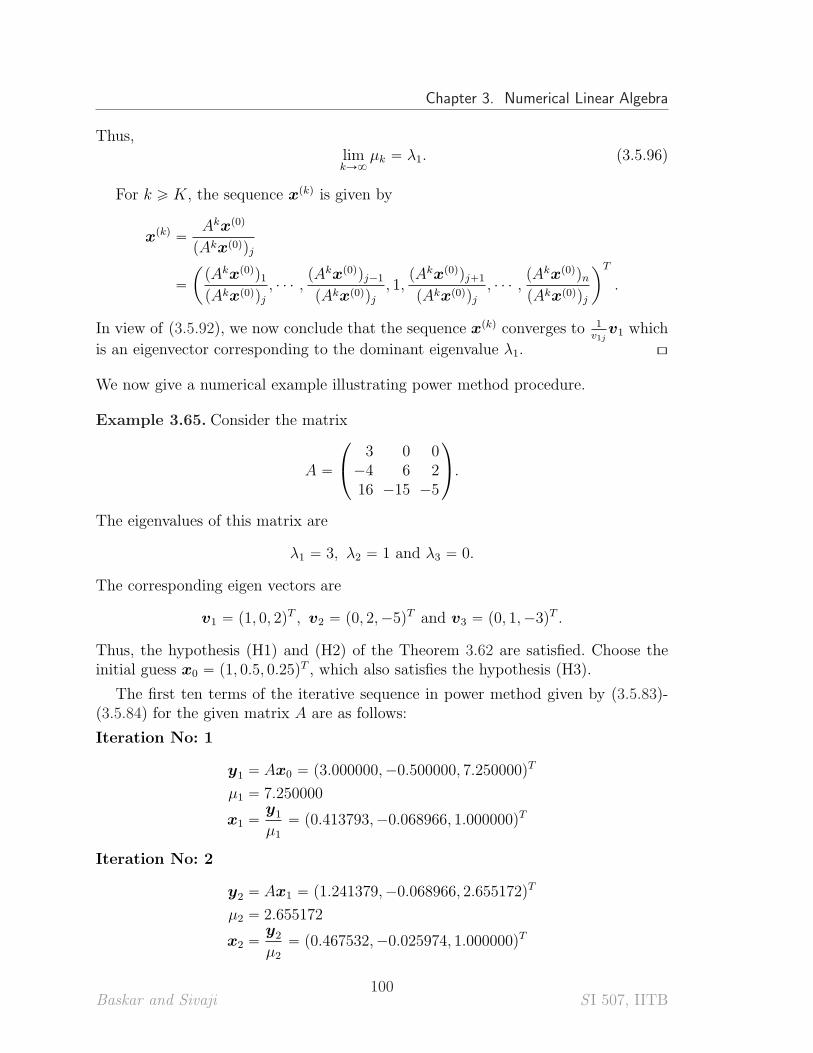
Chapter 3. Numerical Linear Algebra
Thus,limkÑ8
µk “ λ1. (3.5.96)
For k ě K, the sequence xpkq is given by
xpkq “Akxp0q
pAkxp0qqj
“
ˆ
pAkxp0qq1
pAkxp0qqj, ¨ ¨ ¨ ,
pAkxp0qqj´1
pAkxp0qqj, 1,
pAkxp0qqj`1
pAkxp0qqj, ¨ ¨ ¨ ,
pAkxp0qqn
pAkxp0qqj
˙T
.
In view of (3.5.92), we now conclude that the sequence xpkq converges to 1v1j
v1 which
is an eigenvector corresponding to the dominant eigenvalue λ1. [\
We now give a numerical example illustrating power method procedure.
Example 3.65. Consider the matrix
A “
¨
˝
3 0 0´4 6 216 ´15 ´5
˛
‚.
The eigenvalues of this matrix are
λ1 “ 3, λ2 “ 1 and λ3 “ 0.
The corresponding eigen vectors are
v1 “ p1, 0, 2qT , v2 “ p0, 2,´5qT and v3 “ p0, 1,´3qT .
Thus, the hypothesis (H1) and (H2) of the Theorem 3.62 are satisfied. Choose theinitial guess x0 “ p1, 0.5, 0.25qT , which also satisfies the hypothesis (H3).
The first ten terms of the iterative sequence in power method given by (3.5.83)-(3.5.84) for the given matrix A are as follows:
Iteration No: 1
y1 “ Ax0 “ p3.000000,´0.500000, 7.250000qT
µ1 “ 7.250000
x1 “y1
µ1
“ p0.413793,´0.068966, 1.000000qT
Iteration No: 2
y2 “ Ax1 “ p1.241379,´0.068966, 2.655172qT
µ2 “ 2.655172
x2 “y2
µ2
“ p0.467532,´0.025974, 1.000000qT
Baskar and Sivaji100
S I 507, IITB
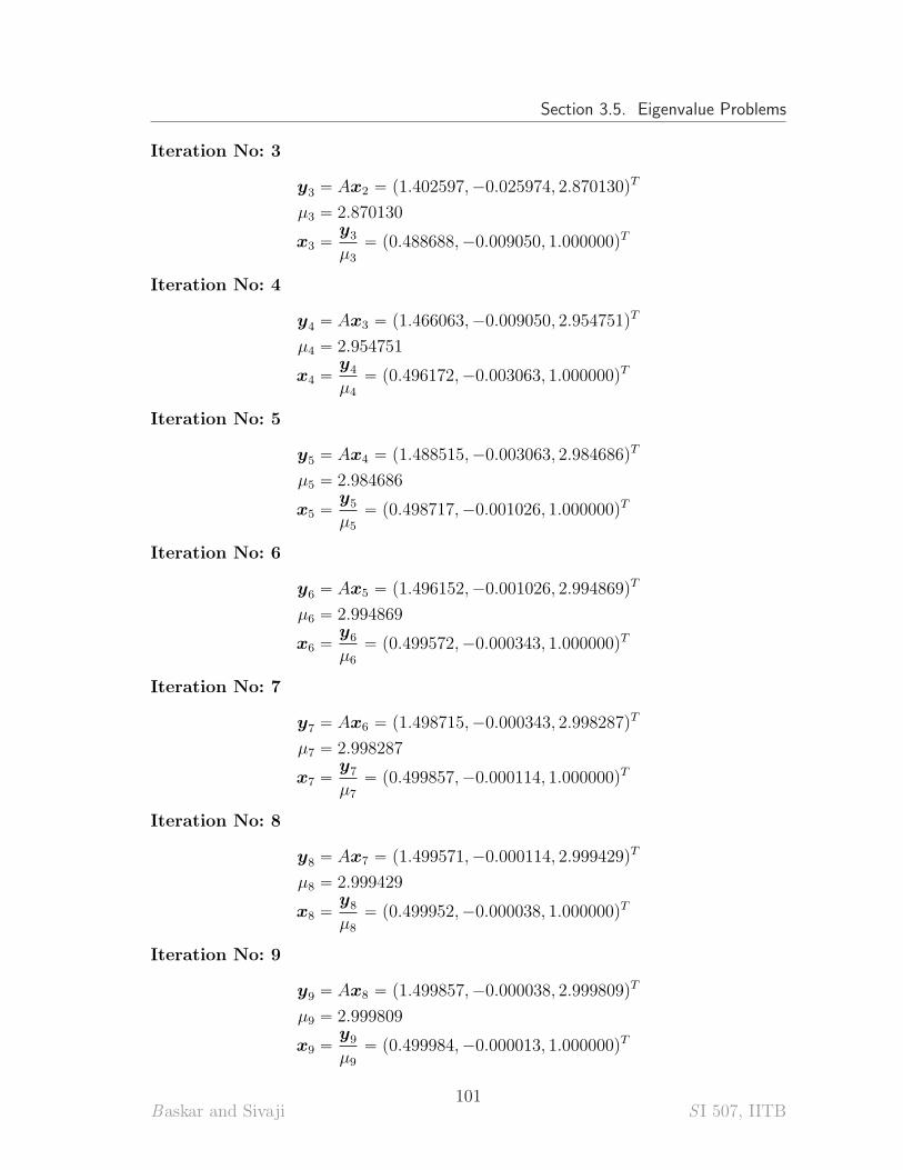
Section 3.5. Eigenvalue Problems
Iteration No: 3
y3 “ Ax2 “ p1.402597,´0.025974, 2.870130qT
µ3 “ 2.870130
x3 “y3
µ3
“ p0.488688,´0.009050, 1.000000qT
Iteration No: 4
y4 “ Ax3 “ p1.466063,´0.009050, 2.954751qT
µ4 “ 2.954751
x4 “y4
µ4
“ p0.496172,´0.003063, 1.000000qT
Iteration No: 5
y5 “ Ax4 “ p1.488515,´0.003063, 2.984686qT
µ5 “ 2.984686
x5 “y5
µ5
“ p0.498717,´0.001026, 1.000000qT
Iteration No: 6
y6 “ Ax5 “ p1.496152,´0.001026, 2.994869qT
µ6 “ 2.994869
x6 “y6
µ6
“ p0.499572,´0.000343, 1.000000qT
Iteration No: 7
y7 “ Ax6 “ p1.498715,´0.000343, 2.998287qT
µ7 “ 2.998287
x7 “y7
µ7
“ p0.499857,´0.000114, 1.000000qT
Iteration No: 8
y8 “ Ax7 “ p1.499571,´0.000114, 2.999429qT
µ8 “ 2.999429
x8 “y8
µ8
“ p0.499952,´0.000038, 1.000000qT
Iteration No: 9
y9 “ Ax8 “ p1.499857,´0.000038, 2.999809qT
µ9 “ 2.999809
x9 “y9
µ9
“ p0.499984,´0.000013, 1.000000qT
Baskar and Sivaji101
S I 507, IITB
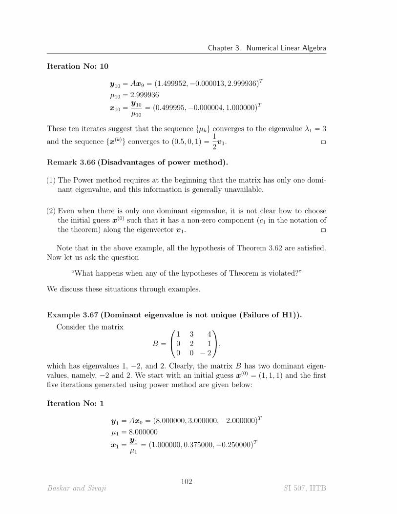
Chapter 3. Numerical Linear Algebra
Iteration No: 10
y10 “ Ax9 “ p1.499952,´0.000013, 2.999936qT
µ10 “ 2.999936
x10 “y10
µ10
“ p0.499995,´0.000004, 1.000000qT
These ten iterates suggest that the sequence tµku converges to the eigenvalue λ1 “ 3
and the sequence txpkqu converges to p0.5, 0, 1q “1
2v1. [\
Remark 3.66 (Disadvantages of power method).
(1) The Power method requires at the beginning that the matrix has only one domi-nant eigenvalue, and this information is generally unavailable.
(2) Even when there is only one dominant eigenvalue, it is not clear how to choosethe initial guess xp0q such that it has a non-zero component (c1 in the notation ofthe theorem) along the eigenvector v1. [\
Note that in the above example, all the hypothesis of Theorem 3.62 are satisfied.Now let us ask the question
“What happens when any of the hypotheses of Theorem is violated?”
We discuss these situations through examples.
Example 3.67 (Dominant eigenvalue is not unique (Failure of H1)).
Consider the matrix
B “
¨
˝
1 3 40 2 10 0 ´ 2
˛
‚,
which has eigenvalues 1, ´2, and 2. Clearly, the matrix B has two dominant eigen-values, namely, ´2 and 2. We start with an initial guess xp0q “ p1, 1, 1q and the firstfive iterations generated using power method are given below:
Iteration No: 1
y1 “ Ax0 “ p8.000000, 3.000000,´2.000000qT
µ1 “ 8.000000
x1 “y1
µ1
“ p1.000000, 0.375000,´0.250000qT
Baskar and Sivaji102
S I 507, IITB
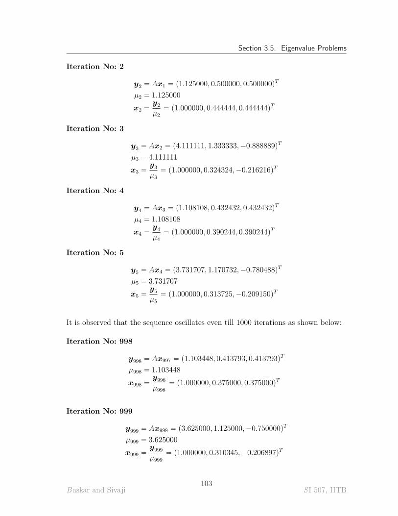
Section 3.5. Eigenvalue Problems
Iteration No: 2
y2 “ Ax1 “ p1.125000, 0.500000, 0.500000qT
µ2 “ 1.125000
x2 “y2
µ2
“ p1.000000, 0.444444, 0.444444qT
Iteration No: 3
y3 “ Ax2 “ p4.111111, 1.333333,´0.888889qT
µ3 “ 4.111111
x3 “y3
µ3
“ p1.000000, 0.324324,´0.216216qT
Iteration No: 4
y4 “ Ax3 “ p1.108108, 0.432432, 0.432432qT
µ4 “ 1.108108
x4 “y4
µ4
“ p1.000000, 0.390244, 0.390244qT
Iteration No: 5
y5 “ Ax4 “ p3.731707, 1.170732,´0.780488qT
µ5 “ 3.731707
x5 “y5
µ5
“ p1.000000, 0.313725,´0.209150qT
It is observed that the sequence oscillates even till 1000 iterations as shown below:
Iteration No: 998
y998 “ Ax997 “ p1.103448, 0.413793, 0.413793qT
µ998 “ 1.103448
x998 “y998
µ998
“ p1.000000, 0.375000, 0.375000qT
Iteration No: 999
y999 “ Ax998 “ p3.625000, 1.125000,´0.750000qT
µ999 “ 3.625000
x999 “y999
µ999
“ p1.000000, 0.310345,´0.206897qT
Baskar and Sivaji103
S I 507, IITB
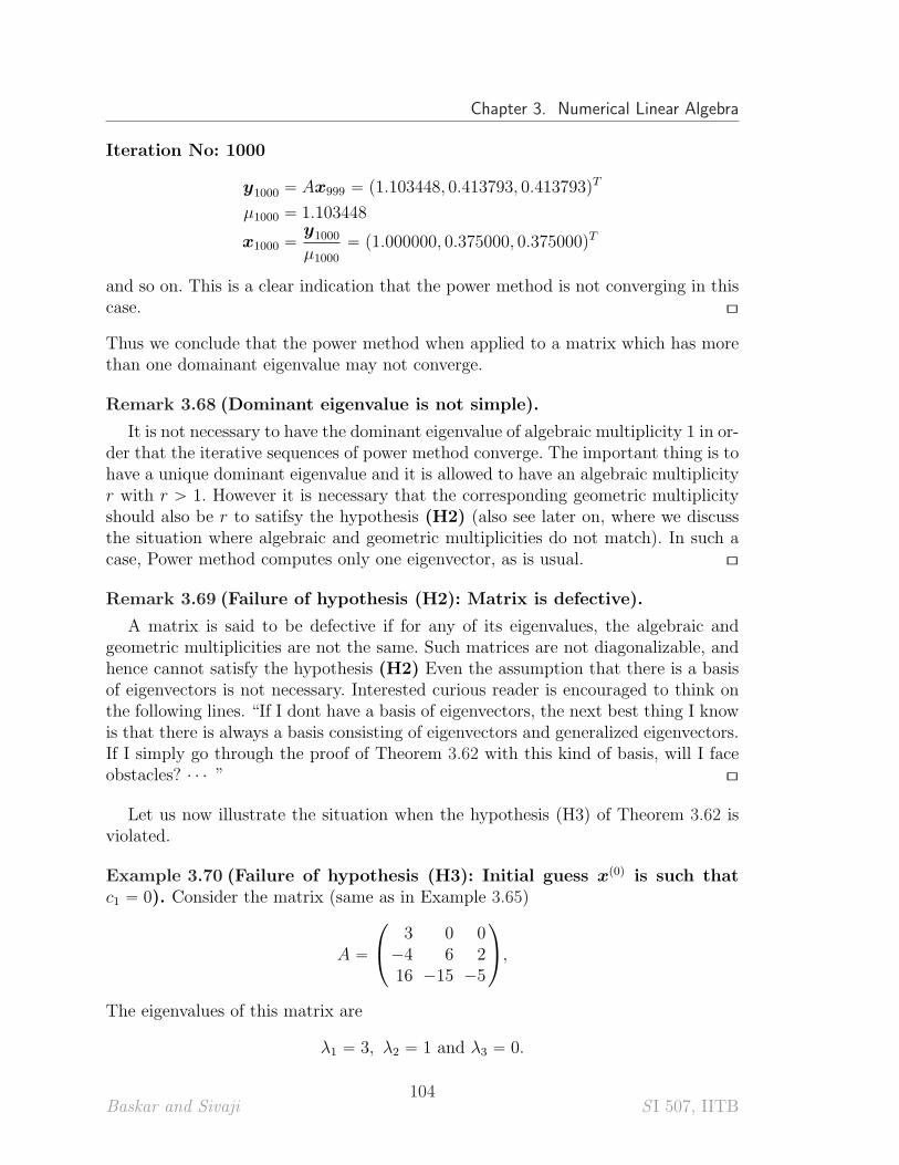
Chapter 3. Numerical Linear Algebra
Iteration No: 1000
y1000 “ Ax999 “ p1.103448, 0.413793, 0.413793qT
µ1000 “ 1.103448
x1000 “y1000
µ1000
“ p1.000000, 0.375000, 0.375000qT
and so on. This is a clear indication that the power method is not converging in thiscase. [\
Thus we conclude that the power method when applied to a matrix which has morethan one domainant eigenvalue may not converge.
Remark 3.68 (Dominant eigenvalue is not simple).
It is not necessary to have the dominant eigenvalue of algebraic multiplicity 1 in or-der that the iterative sequences of power method converge. The important thing is tohave a unique dominant eigenvalue and it is allowed to have an algebraic multiplicityr with r ą 1. However it is necessary that the corresponding geometric multiplicityshould also be r to satifsy the hypothesis (H2) (also see later on, where we discussthe situation where algebraic and geometric multiplicities do not match). In such acase, Power method computes only one eigenvector, as is usual. [\
Remark 3.69 (Failure of hypothesis (H2): Matrix is defective).
A matrix is said to be defective if for any of its eigenvalues, the algebraic andgeometric multiplicities are not the same. Such matrices are not diagonalizable, andhence cannot satisfy the hypothesis (H2) Even the assumption that there is a basisof eigenvectors is not necessary. Interested curious reader is encouraged to think onthe following lines. “If I dont have a basis of eigenvectors, the next best thing I knowis that there is always a basis consisting of eigenvectors and generalized eigenvectors.If I simply go through the proof of Theorem 3.62 with this kind of basis, will I faceobstacles? ¨ ¨ ¨ ” [\
Let us now illustrate the situation when the hypothesis (H3) of Theorem 3.62 isviolated.
Example 3.70 (Failure of hypothesis (H3): Initial guess xp0q is such thatc1 “ 0). Consider the matrix (same as in Example 3.65)
A “
¨
˝
3 0 0´4 6 216 ´15 ´5
˛
‚,
The eigenvalues of this matrix are
λ1 “ 3, λ2 “ 1 and λ3 “ 0.
Baskar and Sivaji104
S I 507, IITB
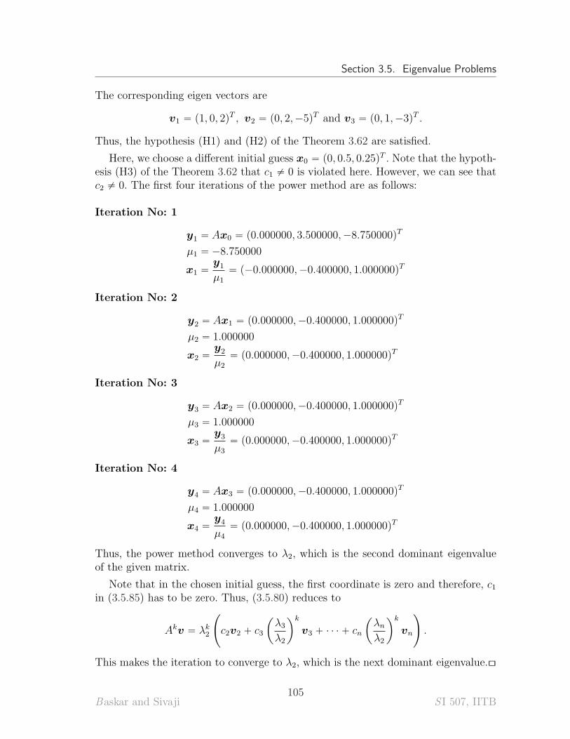
Section 3.5. Eigenvalue Problems
The corresponding eigen vectors are
v1 “ p1, 0, 2qT , v2 “ p0, 2,´5qT and v3 “ p0, 1,´3qT .
Thus, the hypothesis (H1) and (H2) of the Theorem 3.62 are satisfied.
Here, we choose a different initial guess x0 “ p0, 0.5, 0.25qT . Note that the hypoth-esis (H3) of the Theorem 3.62 that c1 ‰ 0 is violated here. However, we can see thatc2 ‰ 0. The first four iterations of the power method are as follows:
Iteration No: 1
y1 “ Ax0 “ p0.000000, 3.500000,´8.750000qT
µ1 “ ´8.750000
x1 “y1
µ1
“ p´0.000000,´0.400000, 1.000000qT
Iteration No: 2
y2 “ Ax1 “ p0.000000,´0.400000, 1.000000qT
µ2 “ 1.000000
x2 “y2
µ2
“ p0.000000,´0.400000, 1.000000qT
Iteration No: 3
y3 “ Ax2 “ p0.000000,´0.400000, 1.000000qT
µ3 “ 1.000000
x3 “y3
µ3
“ p0.000000,´0.400000, 1.000000qT
Iteration No: 4
y4 “ Ax3 “ p0.000000,´0.400000, 1.000000qT
µ4 “ 1.000000
x4 “y4
µ4
“ p0.000000,´0.400000, 1.000000qT
Thus, the power method converges to λ2, which is the second dominant eigenvalueof the given matrix.
Note that in the chosen initial guess, the first coordinate is zero and therefore, c1in (3.5.85) has to be zero. Thus, (3.5.80) reduces to
Akv “ λk2
˜
c2v2 ` c3
ˆ
λ3λ2
˙k
v3 ` ¨ ¨ ¨ ` cn
ˆ
λnλ2
˙k
vn
¸
.
This makes the iteration to converge to λ2, which is the next dominant eigenvalue.[\
Baskar and Sivaji105
S I 507, IITB
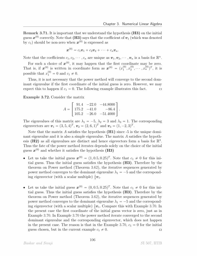
Chapter 3. Numerical Linear Algebra
Remark 3.71. It is important that we understand the hypothesis (H3) on the initialguess xp0q correctly. Note that (H3) says that the coefficient of v1 (which was denotedby c1) should be non-zero when xp0q is expressed as
xp0q “ c1v1 ` c2v2 ` ¨ ¨ ¨ ` cnvn.
Note that the coefficients c1, c2, ¨ ¨ ¨ , cn are unique as v1,v2, ¨ ¨ ¨ ,vn is a basis for Rn.
For such a choice of xp0q, it may happen that the first coordinate may be zero.That is, if xp0q is written in coordinate form as xp0q “ px
p0q
1 , xp0q
2 , ¨ ¨ ¨ , xp0qn qT , it is
possible that xp0q
1 “ 0 and c1 ‰ 0.
Thus, it is not necessary that the power method will converge to the second dom-inant eigenvalue if the first coordinate of the initial guess is zero. However, we mayexpect this to happen if c1 “ 0. The following example illustrates this fact. [\
Example 3.72. Consider the matrix
A “
»
–
91.4 ´22.0 ´44.8000175.2 ´41.0 ´86.4105.2 ´26.0 ´51.4000
fi
fl .
The eigenvalues of this matrix are λ1 “ ´5, λ2 “ 3 and λ3 “ 1. The correspondingeigenvectors are v1 “ p3, 5, 4qT , v2 “ p2, 6, 1qT and v3 “ p1,´2, 3qT .
Note that the matrix A satisfies the hypothesis (H1) since -5 is the unique domi-nant eigenvalue and it is also a simple eigenvalue. The matrix A satisfies the hypoth-esis (H2) as all eigenvalues are distinct and hence eigevectors form a basis for R3.Thus the fate of the power method iterates depends solely on the choice of the initialguess xp0q and whether it satisfies the hypothesis (H3)
• Let us take the initial guess xp0q “ p1, 0.5, 0.25qT . Note that c1 ‰ 0 for this ini-tial guess. Thus the initial guess satisfies the hypothesis (H3). Therefore by thetheorem on Power method (Theorem 3.62), the iterative sequences generated bypower method converges to the dominant eigenvalue λ1 “ ´5 and the correspond-ing eigenvector (with a scalar multiple) 1
5v1.
• Let us take the initial guess xp0q “ p0, 0.5, 0.25qT . Note that c1 ‰ 0 for this ini-tial guess. Thus the initial guess satisfies the hypothesis (H3). Therefore by thetheorem on Power method (Theorem 3.62), the iterative sequences generated bypower method converges to the dominant eigenvalue λ1 “ ´5 and the correspond-ing eigenvector (with a scalar multiple) 1
5v1. Compare this with Example 3.70. In
the present case the first coordinate of the initial guess vector is zero, just as inExample 3.70. In Example 3.70 the power method iterate converged to the seconddominant eigenvalue and the corresponding eigenvector, which does not happenin the present case. The reason is that in the Example 3.70, c1 “ 0 for the initialguess chosen, but in the current example c1 ‰ 0. [\
Baskar and Sivaji106
S I 507, IITB
Section 3.5. Eigenvalue Problems
3.5.2 Gerschgorin’s Theorem
An important tool in eigenvalue approximation is the ability to localize the eigenval-ues, and the most important tool in eigenvalue localization is Gerschgorin’s theorem.Gerschgorin’s Circle theorem helps us in localization of eigenvalues of a matrix. Thistheorem explicitly constructs n disks in the complex plane with centers at the diag-onal elements of the matrix; and all the eigenvalues of the matrix lie in the union ofthese disks.
Theorem 3.73 (Gerschgorin’s Circle Theorem). Let A be an nˆn matrix. Foreach k “ 1, 2, ¨ ¨ ¨ , n, define ρk by
ρk “
nÿ
j“1j‰k
|akj|,
and Dk denotes the closed disk in the complex plane with centre akk and radius ρk,i.e.,
Dk “␣
z P C : |z ´ akk| ď ρk(
.
(1) Each eigenvalue of A lies in one of the disks Dk. That is, no eigenvalue of A liesin Cz Yn
k“1 Dk.
(2) Suppose that among the disks D1, D2, ¨ ¨ ¨ , Dn, there is a collection of m diskswhose union (denoted by R1) is disjoint from the union of the rest of the n´m disks(denoted by R2). Then exactly m eigenvalues lie in R1 and n´m eigenvalues lie inR2 (here each eigenvalue is counted as many times as its algebraic multiplicity).
Proof. We will prove only (i) as it is easy, and the proving (ii) is beyond the scopeof this course.
Let λ be an eigenvalue of A. Then there exists a v “ pv1, v2, ¨ ¨ ¨ , vnq P Rn and v ‰ 0such that
Av “ λv (3.5.97)
Let 1 ď r ď n be such that |vr| “ maxt|v1|, |v2|, ¨ ¨ ¨ , |vn|u. The rth equation of thesystem of equations (3.5.97) is given by (actually, of Av ´ λv “ 0)
ar1v1 ` ¨ ¨ ¨ ` ar,r´1vr´1 ` parr ´ λqvr ` ar,r`1vr`1 ` ¨ ¨ ¨ ` arnvn “ 0
From the last equation, we get
λ ´ arr “v1vrar1 ` ¨ ¨ ¨ `
vr´1
vrar,r´1 `
vr`1
vrar,r`1 ` ¨ ¨ ¨ `
vnvrarn (3.5.98)
Taking modulus on both sides of the equation (3.5.98), and using the triangle in-equality |a ` b| ď |a| ` |b| repeatedly we get
Baskar and Sivaji107
S I 507, IITB
Chapter 3. Numerical Linear Algebra
|λ ´ arr| ď|v1|
|vr||ar1| ` ¨ ¨ ¨ `
|vr´1|
|vr||ar,r´1| `
|vr`1|
|vr||ar,r`1| ` ¨ ¨ ¨ `
|vn|
|vr||arn| (3.5.99)
In view of the choice of r, the components of the vector v satisfy |vs|
|vr|ď 1. The last
equation (3.5.99) becomes
|λ ´ arr| ď |ar1| ` ¨ ¨ ¨ ` |ar,r´1| ` |ar,r`1| ` ¨ ¨ ¨ ` |arn| (3.5.100)
Observe that the right hand side of the inequality (3.5.100) is ρr. This proves thatλ P Dr. [\
Example 3.74. For the matrix¨
˝
4 1 10 2 1
´2 0 9
˛
‚,
the Gerschgorin’s disks are given by
D1 “␣
z P C : |z´4| ď 2(
, D2 “␣
z P C : |z´2| ď 1(
, D3 “␣
z P C : |z´9| ď 2(
.
Draw a picture of these disks and observe that D3 neither intersects D1 nor D2. By(ii) of Theorem 3.73, D3 has one eigenvalue and D1YD2 has two eigenvalues countingmultiplicities. Note that the eigenvalues are approximately 4.6318, 1.8828 P D1 YD2
and 8.4853 P D3. [\
Remark 3.75. Gerschgorin’s circle theorem is helpful in finding bound for eigenval-ues. For the matrix in Example 3.74, any number z in D1 satisfies |z| ď 6. Similarlyany number z in D2 satisfies |z| ď 3, and any number z in D3 satisfies |z| ď 11. Sinceany eigenvalue λ lies in one of three disks, we can conclude that |λ| ď 11. [\
Remark 3.76. The main disadvantage of the power method discussed in Section3.5.1 is that if a given matrix has more than one dominant eigenvalues, then themethod may not converge. So, for a given matrix, we do not know whether the powermethod will converge or not. Also, as the power method is reasonably slow (seeExample 3.72 for an illustration) we may have to perform reasonably large numberof iterations to come to know that the method is not actually converging.
Thus, a tool to find out whether the given matrix has a unique dominant eigenvalueor not is highly desirable. The Gerschgorin theorem 3.73 can sometime be used to seeif power method can be used for a given matrix. For instance, in Example 3.74, wesee that the power method can be used to obtain an approximation to the dominanteigenvalue. [\
Since the matrices A and its transpose (denoted by AT ) have same eigenvalues, wecan apply Gerschgorin Circle Theorem to AT and conclude the following corollary.
Baskar and Sivaji108
S I 507, IITB
Section 3.5. Eigenvalue Problems
Corollary 3.77. Let A be an n ˆ n matrix. For each k “ 1, 2, ¨ ¨ ¨ , n, define τk by
τk “
nÿ
j“1j‰k
|ajk|,
and Bk denotes the closed disk in the complex plane with centre akk and radius τk.That is,
Bk “␣
z P C : |z ´ akk| ď τk(
.
(1) Each eigenvalue of A lies in one of the disks Bk. That is, no eigenvalue of A liesin Cz Yn
k“1 Bk.
(2) Suppose that among the disks B1, B2, ¨ ¨ ¨ , Bn, there is a collection of m disks whoseunion (denoted by C1) is disjoint from the union of the rest of the n ´ m disks(denoted by C2). Then exactly m eigenvalues lie in C1 and n´m eigenvalues lie inC2 (here each eigenvalue is counted as many times as its algebraic multiplicity).[\
Remark 3.78. Advantage of the above corollary is the following: Let A be an nˆ nmatrix. Let R denote the region defined by R “ Yn
k“1Dk where Dk are as given byTheorem 3.73. Similarly, let C denote the region defined by C “ Yn
k“1Bk where Bk
are as given by Corollary 3.77. It may happen that C Ă R, in which case we will getbetter estimate for eigenvalues of A. It may not happen for every matrix A. Howeverwhenever such a thing happens, we get better bounds for eigenvalues of A. Suchbounds which we obtain using both informations R and C may be called optimumbounds. Let us illustrate this with two examples. [\
Example 3.79. For the matrix
¨
˝
3 0 10 ´2 20 2 ´3
˛
‚
the ρk, τk (in the notations of Theorem 3.73 and Corollary 3.77) are given by
ρ1 “ 1, ρ2 “ 2, ρ3 “ 3, and τ1 “ 0, τ2 “ 2, τ3 “ 3
Now compute
R “ Ynk“1Dk “ tz : |z ´ 3| ď 1u Y tz : |z ` 2| ď 2u Y tz : |z ` 3| ď 3u
C “ Ynk“1Bk “ tz : |z ´ 3| ď 0u Y tz : |z ` 2| ď 2u Y tz : |z ` 3| ď 3u
and clearly C Ă R. Hence bounds obtained using C are optimum bounds. Draw bothregions C and R. [\
Baskar and Sivaji109
S I 507, IITB
Chapter 3. Numerical Linear Algebra
3.6 Exercises
Gaussian Elimination Methods
(1) Solve the following systems of linear equations using Naive Gaussian eliminationmethod, and modified Gaussian elimination method with partial pivoting.
(i)
6x1 ` 2x2 ` 2x3 “ ´2,
2x1 ` 0.6667x2 ` 0.3333x3 “ 1,
x1 ` 2x2 ´ x3 “ 0.
(ii)
0.729x1 ` 0.81x2 ` 0.9x3 “ 0.6867,
x1 ` x2 ` x3 “ 0.8338,
1.331x1 ` 1.21x2 ` 1.1x3 “ 1
(iii)
x1 ´ x2 ` 3x3 “ 2,
3x1 ´ 3x2 ` x3 “ ´1,
x1 ` x2 “ 3.
(2) Solve the system0.001x1 ` x2 “ 1, x1 ` x2 “ 2
(i) using Gaussian elimination with partial pivoting with infinite precision arith-metic,
(ii) using naive Gaussian elimination with 2-digit rounding, and
(iii) using modified Gaussian elimination method with partial pivoting, using 2-digit rounding.
(3) Let ϵ be such that 0 ă ϵ ! 1. Solve the linear system
x1 ` x2 ` x3 “ 6,
3x1 ` p3 ` ϵqx2 ` 4x3 “ 20,
2x1 ` x2 ` 3x3 “ 13
using naive Gaussian elimination method, and using modified Gaussian elimina-tion method with partial pivoting. Obtain the residual error in each case on acomputer for which the ϵ is less than its machine epsilon. The residual error vec-tor corresponding to an approximate solution x˚ is defined as r “ b´Ax˚, where
Baskar and Sivaji110
S I 507, IITB
Section 3.6. Exercises
A and b are the coefficient matrix and the right side vector, respectively, of thegiven linear system.
(4) A matrix A “ paijq is said to be row-equilibrated if the following condition issatisfied
max1ďjďn
|aij| “ 1 @i “ 1, 2, ¨ ¨ ¨ , n.
Consider the following system of linear equations
30.00x1 ` 591400x2 “ 591700
5.291x1 ´ 6.130x2 “ 46.78
(i) Find the exact solution of the given system using Gaussian elimination methodwith partial pivoting (i.e., with infinite precision arithmetic).
(ii) Solve the given system using naive Gaussian elimination method using 4-digitrounding.
(iii) Obtain a system of linear equations rAx “ rb that is equivalent to the given
system, where the matrix rA is row-equilibrated. Solve the system rAx “ rbusing naive Gaussian elimination method using 4-digit rounding.
(iv) Compute the relative errors involved in the two approximations obtainedabove.
(5) Consider the system of linear equations given by
a11x1` ¨ ¨ ¨ `a1nxn “ b1,
¨ ¨ ¨
¨ ¨ ¨
an1x1` ¨ ¨ ¨ `annxn “ bn,
where aij “ 0 whenever i ´ j ě 2. Write the general form of this system. Usenaive Gaussian elimination method to solve it, taking advantage of the elementsthat are known to be zero. Count the number of operations involved in this com-putation.
(6) Use Thomas method to solve the tri-diagonal system of equations
2x1 ` 3x2 “ 1,
x1 ` 2x2 ` 3x3 “ 4,
x2 ` 2x3 ` 3x4 “ 5,
x3 ` 2x4 “ 2.
Baskar and Sivaji111
S I 507, IITB
Chapter 3. Numerical Linear Algebra
LU Decomposition
(7) Prove or disprove the following statements:
(i) An invertible matrix has at most one Doolittle factorization.
(ii) If a singular matrix has a Doolittle factorization, then the matrix has at leasttwo Doolittle factorizations.
(8) Prove that if an invertible matrix A has an LU -factorization, then all principalminors of A are non-zero.
(9) Give an example of a non-invertible 3ˆ3 matrix A such that the leading principalminors of order 1 and 2 are non-zero, and A has Doolittle factorization.
(10) Use the Doolittle’s factorization to solve the system
4x1 ` x2 ` x3 “ 4,
x1 ` 4x2 ´ 2x3 “ 4,
3x1 ` 2x2 ´ 4x3 “ 6.
(11) Show that the matrix¨
˝
2 2 11 1 13 2 1
˛
‚
is invertible but has no LU factorization. Do a suitable interchange of rows to getan invertible matrix, which has an LU factorization.
(12) Consider
A “
¨
˝
2 6 ´46 17 ´17
´4 ´17 ´20
˛
‚.
Determine directly the factorization A “ LDLT , where D is diagonal and L is alower triangular matrix with 1’s on its diagonal.
(13) Let A be an nˆn matrix which is positive definite. Let S be a non-empty susbsetof t1, 2, ¨ ¨ ¨ , nu. Show that the submatrix AS “ paijqi,jPS is positive definite.
(14) Factor the matrix
A “
¨
˝
4 6 26 10 32 3 5
˛
‚
so that A “ LLT , where L is lower triangular.
Baskar and Sivaji112
S I 507, IITB
Section 3.6. Exercises
(15) Prove the uniqueness of the factorization A “ LLT , where L is a lower tri-angular matrix all of whose diagonal entries are positive. (Hint: Assume thatthere are lower triangular matrices L1 and L2 with positive diagonals. Prove thatL1L
´12 “ I.)
(16) Use Cholesky factorization to solve the system of equations
x1 ´ 2x2 ` 2x3 “ 4,
´2x1 ` 5x2 ´ 3x3 “ ´7,
2x1 ´ 3x2 ` 6x3 “ 10.
Matrix Norms
(17) The following inequalities show that the notion of convergent sequences of vectorsin Rn is independent of the vector norm. Show that the following inequalities holdfor each x P Rn
(i) }x}8 ď }x}2 ď?n}x}8,
(ii) }x}8 ď }x}1 ď n}x}8,
(iii) }x}2 ď }x}1 ď?n}x}2.
(18) Show that the norm defined on the set of all n ˆ n matrices by
}A} :“ max1ďiďn1ďjďn
|aij|
is not subordinate to any vector norm on Rn.
(19) Let A be an invertible matrix. Show that its condition number κpAq satisfiesκpAq ě 1.
(20) Let A and B be invertible matrices with condition numbers κpAq and κpBq re-spectively. Show that κpABq ď κpAqκpBq.
(21) Let A be an n ˆ n matrix with real entries. Let κ2pAq and κ8pAq denote thecondition numbers of a matrix A that are computed using the matrix norms }A}2and }A}8, respectively. Answer the following questions.
(i) Determine all the diagonal matrices such that κ8pAq “ 1.
(ii) Let Q be a matrix such that QTQ “ I (such matrices are called orthogonalmatrices). Show that κ2pQq “ 1.
(iii) If κ2pAq “ 1, show that all the eigenvalues of ATA are equal. Further, deducethat A is a scalar multiple of an orthogonal matrix.
Baskar and Sivaji113
S I 507, IITB
Chapter 3. Numerical Linear Algebra
(22) Let Apαq be a matrix depending on a parameter α P R given by
Apαq “
ˆ
0.1α 0.1α1.0 2.5
˙
For each α P R, compute the condition number of Apαq. Determine an α0 suchthat the condition number of Apα0q is the minimum of the set tκ pApαqq : α P Ru.In the computation of condition numbers, use the matrix norm that is subordinateto the maximum vector norm on R2.
(23) In solving the system of equations Ax “ b with matrix
A “
ˆ
1 21 2.01
˙
,
predict how slight changes in b will affect the solution x. Test your prediction inthe concrete case when b “ p4, 4qT and b “ p3, 5qT . Use the maximum norm forvectors in R2.
(24) Consider the following two systems of linear equations
x1 ` x2 “ 1, x1 ` 2x2 “ 2.
and10´4 x1 ` 10´4 x2 “ 10´4, x1 ` 2x2 “ 2.
Let us denote the first and second systems by A1x “ b1 and A2x “ b2 respectively.Use maximum-norm for vectors and the matrix norm subordinate to maximum-norm for matrices in your computations.
(i) Solve each of the above systems using Naive Gaussian elimination method.
(ii) Compute the condition numbers of A1 and A2.
(iii) For each of the systems, find an upper bound for the relative error in the
solution if the right hand sides are approximated by Ăb1 and Ăb2 respectively.
(iv) Solve the systems
A1x “ Ăb1 and A2x “ Ăb2
where Ăb1 “ p1.02, 1.98qT and Ăb2 “ p1.02 ˆ 10´4, 1.98qT using naive Gaussianelimination method. Compute the relative error in each case. Compare thecomputed relative errors with the bounds obtained above.
(25) In the following problems, the matrix norm }¨} denotes a matrix norm subordinateto a fixed vector norm.
(i) Let A be an invertible matrix andB be any singular matrix. Prove the followinginequality.
1
}A ´ B}ď }A´1}.
Baskar and Sivaji114
S I 507, IITB
Section 3.6. Exercises
(ii) Let A be an invertible matrix, and B be a matrix such that
1
}A ´B}ą }A´1}.
Show that B is invertible.
(iii) Let C be a matrix such that }I ´ C} ă 1. Show that C is invertible.
(iv) Let D be a matrix such that }D} ă 1. Show that the matrix I´D is invertible.
Diagonally Dominant Matrix
(26) Let A be a diagonally dominant matrix. Then show that Naive Gaussian elimina-tion method to solve the system of linear equations Ax “ b never fails to give anapproximate solution of the given linear system.
(27) Let A be a diagonally dominant matrix such that aij “ 0 for every i, j P
t1, 2, ¨ ¨ ¨ , nu such that i ą j`1. Does naive Gaussian elimination method preservethe diagonal dominance? Justify your answer.
Iterative Methods
(28) Let A be a diagonally dominant matrix. Show that all the diagonal elements ofA are non-zero (i.e., aii ‰ 0 for i “ 1, 2, ¨ ¨ ¨ , n.). As a consequence, the iteratingsequences of Jacobi and Gauss-Seidel methods are well-defined if the coefficientmatrix A in the linear system Ax “ b is a diagonally dominant matrix.
(29) Find the nˆnmatrix B and the n-dimensional vector c such that the Gauss-Seidalmethod can be written in the form
xpk`1q “ Bxpkq ` c, k “ 0, 1, 2, ¨ ¨ ¨
(30) For each of the following systems, write down the formula for iterating sequencesof Jacobi and Gauss-Seidel methods. Compute three iterates by taking x0 “
p0, 0, 0qT . Discuss if you can guarantee that these sequences converge to the exactsolution. In case you are not sure about convergence, suggest another iteratingsequence that converges to the exact solution if possible; and justify that the newsequence converges to the exact solution.
(i)
5x1 ` 2x2 ` x3 “ 0.12,
1.75x1 ` 7x2 ` 0.5x3 “ 0.1,
x1 ` 0.2x2 ` 4.5x3 “ 0.5.
Baskar and Sivaji115
S I 507, IITB
Chapter 3. Numerical Linear Algebra
(ii)
x1 ´ 2x2 ` 2x3 “ 1,
x1 ` x2 ´ x3 “ 1,
2x1 ´ 2x2 ` x3 “ 1.
(iii)
x1 ` x2 ` 10x3 “ ´1,
2x1 ` 3x2 ` 5x3 “ ´6,
3x1 ` 2x2 ´ 3x3 “ 4.
(31) Consider the following system of linear equations
0.8647x1 ` 0.5766x2 “ 0.2885,
0.4322x1 ` 0.2882x2 “ 0.1442.
(i) Find the exact solution of the linear system.
(ii) Using 4-digit chopping, do one iteration of residual corrector method to obtainxp1q. Use the initial guess to be p0, 0qT .
(iii) Compute the residual vector for the solution obtained in (ii) above.
Eigenvalue Problems
(32) The matrix
A “
¨
˝
2 0 02 1 03 0 1
˛
‚
has eigenvalues λ1 “ 2, λ “ 1 and λ3 “ 1 and the corresponding eigenvectorsmay be taken as v1 “ p1, 2, 3qT , v2 “ p0, 1, 2qT and v3 “ p0, 2, 1qT . Perform3 iterations to find the eigenvalue and the corresponding eigen vector to whichthe power method converges when we start the iteration with the initial guessxp0q “ p0, 0.5, 0.75qT . Without performing the iteration, find the eigenvalue andthe corresponding eigenvector to which the power method converges when we startthe iteration with the initial guess xp0q “ p0.001, 0.5, 0.75qT . Justify your answer.
(33) The matrix
A “
¨
˝
5.4 0 0´113.0233 ´0.5388 ´0.6461´46.0567 ´6.4358 ´0.9612
˛
‚
Baskar and Sivaji116
S I 507, IITB
Section 3.6. Exercises
has eigenvalues λ1 “ 5.4, λ2 “ 1.3 and λ3 “ ´2.8 with corresponding eigenvectorsv1 “ p0.2,´4.1, 2.7qT , v2 “ p0, 1.3,´3.7qT and v3 “ p0, 2.6, 9.1qT . To whicheigenvalue and the corresponding eigenvector does the power method convergeif we start with the initial guess xp0q “ p0, 1, 1q? Justify your answer.
(34) Use Gerschgorin’s circle theorem to determine the intervals in which the eigenval-ues of the matrix
A “
¨
˝
0.5 0 0.20 3.15 ´1
0.57 0 ´7.43
˛
‚.
lie, given that all eigenvalues of A are real. Show that power method can beapplied for this matrix to find the dominant eigenvalue without computing eigen-values explicitly. Compute the first three iterates of Power method sequences.
(35) For this question, we take the matrix
A “
¨
˝
´2.7083 ´2.6824 0.45430.1913 0.7629 0.1007
´0.3235 ´0.4052 5.0453
˛
‚.
Let v1,v2,v3 denote eigenvectors corresponding to the eigenvalues λ1, λ2, λ3 re-spectively of the matrix A which are given by λ1 « 5.0187, λ2 « ´2.5313, λ3 «
0.6125 and v1 « p0.25, 0.13, 5.02qT ,v2 « p2.53,´0.15, 0.1qT ,v3 « p´0.49, 0.61, 0.02qT .Answer the following questions:
(i) Obtain the Gerschgorin disks associated to the matrix A and pictorially rep-resent them in the complex plane.
(ii) Can Gerschgorin theorem be used to show that the matrix A has a uniquedominant eigenvalue? Justify your answer.
(iii) Define the iterative sequences tµku and xpkq using power method that convergeto λ1 and αv1 for some constant α when the initial guess is xp0q “ p1, 1, 1qT .Perform one iteration.
(iv) If we take the initial guess xp0q “ p0, 1, 1qT , then show that the iterativesequence obtained by power method converges to λj and Kvj for somej P t1, 2, 3u and for some constant K. What is the value of j and possiblevalues of K?(Hint: xp0q « 0.3060v1 ` 0.1864v2 ` 1.6748v3. )
(v) Give all possible initial guesses for which the sequence tµku obtained usingpower method converges to λ2. Justify your answer.
(vi) Give all possible initial guesses for which the sequence tµku obtained usingpower method converges to λ3. Justify your answer. (End-Sem, Spring2012)
Baskar and Sivaji117
S I 507, IITB
Chapter 3. Numerical Linear Algebra
(36) Use the Gerschgorin Circle theorem to determine bounds for the eigenvalues forthe following matrices. Also find optimum bounds wherever possible. Also drawthe pictures of all the regions given by Greschgorin circles.
¨
˝
1 0 0´1 0 1´1 ´1 2
˛
‚,
¨
˝
4 ´1 0´1 4 ´1´1 ´1 4
˛
‚,
¨
˝
4.75 2.25 ´0.252.25 4.75 1.25
´0.25 1.25 4.75
˛
‚,
¨
˚
˚
˝
1 0 ´1 12 2 ´1 10 1 3 ´21 0 1 4
˛
‹
‹
‚
.
(37) Prove that the following two statements concerning nˆn matrices are equivalent.
(i) Every diagonally dominant matrix is invertible.
(ii) Each of the eigenvalues of a matrix A, belongs to at least one Gerschgorin diskcorresponding to A.
(38) Prove that the eigenvalues of the matrix
¨
˝
6 2 11 ´5 02 1 4
˛
‚
satisfy the inequality 1 ď |λ| ď 9.
(39) Show that the imaginary parts of the eigenvalues of
¨
˝
3 1{3 2{31 ´4 0
1{2 1{2 ´1
˛
‚
all lie in the interval r´1, 1s.
Baskar and Sivaji118
S I 507, IITB
CHAPTER 4
Nonlinear Equations
One of the most frequently occurring problems in practical applications is to find theroots of equations of the form
fpxq “ 0, (4.0.1)
where f : ra, bs Ñ R is a given nonlinear function. It is well-known that not allnonlinear equations can be solved explicitly to obtain the exact value of the rootsand hence, we need to look for methods to compute approximate value of the roots.By approximate root to (4.0.1), we mean a point x˚ P R for which the value fpxq isvery near to zero, ie., fpx˚q « 0.
In this chapter, we introduce various iterative methods to obtain an approximationto a real root of equations of the form (4.0.1) with f being a continuous nonlinearfunction. The key idea in approximating the real roots of (4.0.1) consists of two steps:
(1) Starting Step: Take one or more points (arbitrarily or following a procedure)xi P ra, bs (i “ 0, 1, ¨ ¨ ¨ ,m, m P N) around a root of the equation (4.0.1). Considerxm as an approximation to the root of (4.0.1).
(2) Improving Step: If xm is not ‘close’ to the required root, then devise a procedureto obtain another point xm`1 that is ‘more close’ to the root than xm.
Repeat this step until we obtain a point xn (n ě m) which is ‘sufficiently close’to the required root.
This process of improving the approximation to the root is called the iterative pro-cess (or iterative procedure), and such methods are called iterative methods.In an iterative method, we obtain a sequence of numbers txnu which is expected toconverge to the root of (4.0.1) as n Ñ 8. We investigate conditions on the functionf , its domain, and co-domain under which the sequence of iterates converge to asolution of the equation (4.0.1).
We classify the iterative methods discussed in this chapter into two types, namely,
(1) Closed Domain Methods: As the starting step, these methods need the knowl-edge of an interval in which at least one root of the given nonlinear equation ex-
Chapter 4. Nonlinear Equations
ists. Further iterations include the restriction of this interval to smaller intervalsin which root lies. These methods are also called bracketing methods.
(2) Open Domain Methods: The xi’s mentioned in the starting step above arechosen arbitrarily and the consecutive iterations are based on a formula.
In the case of closed domain methods, the difficult part is to locate an interval con-taining a root. But, once this is done, the iterative sequence will surely converge as wewill see in Section 4.1. In this section, we discuss two closed domain methods, namely,the bisection method and the regula-falsi method. In the case of open domain meth-ods, it is easy at the starting step as we can choose the xi’s arbitrarily. But, it is notnecessary that the sequence converges. We discuss secant method, Newton-Raphsonmethod and fixed point method in Section 4.3, which are some of the open domainmethods.
4.1 Closed Domain Methods
The idea behind the closed domain methods is to start with an interval (denoted byra0, b0s) in which there exists at least one root of the given nonlinear equations andthen reduce the length of this interval iteratively with the condition that there is atleast one root of the equation at each iteration.
Note that the initial interval ra0, b0s can be obtained using the intermediate valuetheorem (as we always assume that the nonlinear function f is continuous) by check-ing the condition that
fpa0qfpb0q ă 0.
That is, fpa0q and fpb0q are of opposite sign. The closed domain methods differ fromeach other only by the way they go on reducing the length of this interval at eachiteration.
In the following subsections we discuss two closed domain methods, namely, (i)the bisection method and (ii) the regula-falsi method.
4.1.1 Bisection Method
The most simple way of reducing the length of the interval is to sub-divide theinterval into two equal parts and then take the sub-interval that contains a root ofthe equation and discard the other part of the interval. This method is called thebisection method. Let us explain the procedure of generating the first iteration ofthis method.
Step 1: Define x1 to be the mid-point of the interval ra0, b0s. That is,
x1 “a0 ` b0
2.
Baskar and Sivaji120
S I 507, IITB
Section 4.1. Closed Domain Methods
Step 2: Now, exactly one of the following two statements hold.
(1) x1 solves the nonlinear equation. That is, fpx1q “ 0.
(2) Either fpa0qfpx1q ă 0 or fpb0qfpx1q ă 0.
If case (1) above holds, then x1 is a required root of the given equation fpxq “ 0 andtherefore we stop the iterative procedure. If fpx1q ‰ 0, then case (2) holds as fpa0qand fpb0q are already of opposite signs. In this case, we define a subinterval ra1, b1sof ra0, b0s as follows.
ra1, b1s “
#
ra0, x1s, if fpa0qfpx1q ă 0,
rx1, b0s, if fpb0qfpx1q ă 0.
The outcome of the first iteration of the bisection method is the interval ra1, b1sand the first member of the corresponding iterative sequence is the real number x1.Observe that
• the length of the interval ra1, b1s is exactly half of the length of ra0, b0s and
• ra1, b1s has at least one root of the nonlinear equation fpxq “ 0.
Similarly, we can obtain x2 and ra2, b2s as the result of the second iteration and soon.
We now present the algorithm for the bisection method.
Hypothesis: There exists an interval ra0, b0s such that the function f : ra0, b0s Ñ Ris continuous, and the numbers fpa0q and fpb0q have opposite signs.
Algorithm:
Step 1: For n “ 0, 1, 2, ¨ ¨ ¨ , define the iterative sequence of the bisection method as
xn`1 “an ` bn
2,
which is the midpoint of the interval ran, bns.
Step 2: One of the following two cases hold.
(1) xn`1 solves the nonlinear equation. That is, fpxn`1q “ 0.
(2) Either fpanqfpxn`1q ă 0 or fpbnqfpxn`1q ă 0.
Define the subinterval ran`1, bn`1s of ran, bns as follows.
ran`1, bn`1s “
#
ran, xn`1s, if fpanqfpxn`1q ă 0,
rxn`1, bns, if fpbnqfpxn`1q ă 0.
Step 3: Stop the iteration if one of the following happens:
Baskar and Sivaji121
S I 507, IITB
Chapter 4. Nonlinear Equations
• the case (1) in step 2 holds. Then declare the value of xn`1 as the required root.
• pbn`1´an`1q is sufficiently small (less than a pre-assigned positive quantity). Thendeclare the value of xn`2 as the required root up to the desired accuracy.
If any of the above stopping criteria does not hold, then go to step 1. Continue thisprocess till one of the above two stopping criteria is fulfilled. [\
Remark 4.1. In practice, one may also use any of the stopping criteria listed insection 4.2, either single or multiple criteria. [\
Assuming that, for each n “ 1, 2, ¨ ¨ ¨ , the number xn is not a solution of thenonlinear equation fpxq “ 0, we get a sequence of real numbers txnu. The question iswhether this sequence converges to a solution of the nonlinear equation fpxq “ 0. Wenow discuss the error estimate and convergence of the iterative sequence generatedby the bisection method.
Theorem 4.2 (Convergence and Error Estimate of Bisection Method).
Hypothesis: Let f : ra0, b0s Ñ R be a continuous function such that the numbersfpa0q and fpb0q have opposite signs.
Conclusion:
• There exists an r P pa0, b0q such that fprq “ 0 and the iterative sequence txnu ofthe bisection method converges to r.
• For each n “ 0, 1, 2, ¨ ¨ ¨ , we have the following error estimate
|xn`1 ´ r| ď
ˆ
1
2
˙n`1
pb0 ´ a0q. (4.1.2)
Proof: It directly follows from the construction of the intervals ran, bns that
bn ´ an “1
2pbn´1 ´ an´1q “ ¨ ¨ ¨ “
ˆ
1
2
˙n
pb0 ´ a0q.
As a consequence, we getlimnÑ8
pbn ´ anq “ 0.
By algebra of limits of sequences, we get
limnÑ8
an “ limnÑ8
bn.
Since for each n “ 0, 1, 2, ¨ ¨ ¨ , the number xn`1 is the mid-point of the interval ran, bns,we also have
an ă xn`1 ă bn.
Baskar and Sivaji122
S I 507, IITB
Section 4.1. Closed Domain Methods
Now by sandwich theorem for sequences, we conclude that the sequence txnu of mid-points also converges to the same limit as the sequences of end-points. Thus we have
limnÑ8
an “ limnÑ8
bn “ limnÑ8
xn “ r (say). (4.1.3)
Since for each n “ 0, 1, 2, ¨ ¨ ¨ , we have fpanqfpbnq ă 0, applying limits on both sidesof the inequality and using the continuity of f , we get
fprqfprq ď 0, (4.1.4)
from which we conclude that fprq “ 0. That is, the sequence of mid-points txnu
defined by the bisection method converges to a root of the nonlinear equation fpxq “
0.
Since the sequences tanu and tbnu are non-decreasing and non-increasing, respec-tively, for each n “ 0, 1, 2, ¨ ¨ ¨ , we have r P ran, bns. Also, xn`1 is the mid-point ofthe interval ran, bns. Therefore, we have
|xn`1 ´ r| ď1
2pbn ´ anq “ ¨ ¨ ¨ “
ˆ
1
2
˙n`1
pb0 ´ a0q,
which is the required estimate. [\
Corollary 4.3. Let ϵ ą 0 be given. Let f satisfy the hypothesis of bisection methodwith the interval ra0, b0s. Let xn be as in the bisection method, and r be the root of thenonlinear equation fpxq “ 0 to which bisection method converges. Then |xn ´ r| ď ϵwhenever n satisfies
n ělogpb0 ´ a0q ´ log ϵ
log 2(4.1.5)
Proof : By the error estimate of bisection method given by (4.1.2), we are sure that
|xn ´ r| ď ϵ,
whenever n is such thatˆ
1
2
˙n
pb0 ´ a0q ď ϵ.
By taking logarithm on both sides of the last inequality, we get the desired estimateon n. [\
Remark 4.4. The Corollary 4.3 tells us that if we want an approximation xn to theroot r of the given equation such that the absolute error is less than a pre-assignedpositive quantity, then we have to perform n iterations, where n is the least integerthat satisfies the inequality (4.1.5). It is interesting to observe that to obtain this n,we don’t need to know the root r. [\
Baskar and Sivaji123
S I 507, IITB
Chapter 4. Nonlinear Equations
Example 4.5. Let us find an approximate solution to the nonlinear equation
sin x ` x2 ´ 1 “ 0
using bisection method so that the resultant absolute error is at most ϵ “ 0.125.
To apply Bisection method, we must choose an interval ra0, b0s such that thefunction
fpxq “ sin x ` x2 ´ 1
satisfies the hypothesis of bisection method. Note that f satisfies hypothesis of bisec-tion on the interval r0, 1s. In order to achieve the required accuracy, we should firstdecide how many iterations are needed. The inequality (4.1.5), says that requiredaccuracy is achieved provided n satisfies
n ělogp1q ´ logp0.125q
log 2“ 3
Thus we have to compute x3. We will do it now.
Iteration 1: We have a0 “ 0, b0 “ 1. Thus x1 “ 0.5. Since,
fpx1q “ ´0.27 ă 0, fp0q ă 0, and fp1q ą 0,
we take ra1, b1s “ rx1, b0s “ r0.5, 1s.
Iteration 2: The mid-point of r0.5, 1s is x2 “ 0.75. Since
fpx2q “ 0.24 ą 0, fp0.5q ă 0, and fp1q ą 0,
we take ra2, b2s “ ra1, x2s “ r0.5, 0.75s.
Iteration 3: The mid-point of r0.5, 0.75s is x3 “ 0.625. Since
fpx3q “ ´0.024 ă 0, fp0.5q ă 0 and fp0.75q ą 0,
we take ra3, b3s “ rx3, b2s “ r0.625, 0.75s.
As suggested by the formula (4.1.5), we stop the iteration here and take the ap-proximate root of the given equation as the mid-point of the interval ra3, b3s, whichis x4 « 0.6875. Note that the true value is r « 0.636733. The absolute error is 0.05which is much less than the required accuracy of 0.125. [\
Remark 4.6 (Comments on Bisection method).
(1) Note that the mid-point of an interval ra, bs is precisely the x´ coordinate of thepoint of intersection of the line joining the points pa, sgnpfpaqqq and pb, sgnpfpbqqq
with the x-axis.
Baskar and Sivaji124
S I 507, IITB
Section 4.1. Closed Domain Methods
(2) Let f , and the interval ra0, b0s satisfy the hypothesis of bisection method. Evenif the nonlinear equation fpxq “ 0 has more than one solution in the intervalra, bs, the bisection method chooses the root that it tries to approximate. In otherwords, once we fix the initial interval ra0, b0s, the bisection method takes over andwe cannot control it to find some specific root than what it chooses to find.
(3) Given a function f , choosing an interval ra, bs such that fpaqfpbq ă 0 is crucial tobisection method. There is no general procedure to find such an interval. This isone of the main drawbacks of bisection method.
(4) Bisection method cannot be used to find zero of functions for which graph touchesx-axis but does not cross x-axis.
(5) There is a misconception about bisection method’s order of convergence (see Def-inition 1.42), which is claimed to be 1. However there is no proof of |xn`1 ´ r| ď
c|xn ´ r|. If the sequence txnu converges linearly to r, then we get
|xn`1 ´ r| ď cn`1|x0 ´ r|.
In the case of bisection method, we have this inequality with c “ 1{2, which isonly a necessary condition for the convergence to be linear but not a sufficientcondition. [\
4.1.2 Regula-falsi Method
The regula-falsi method is similar to the bisection method. Although the bisectionmethod (discussed in the previous subsection) always converges to the solution, theconvergence is very slow, especially when the length of the initial interval ra0, b0s isvery large and the equation has the root very close to the one of the end points.This is because, at every iteration, we are subdividing the interval ran, bns into twoequal parts and taking the mid-point as xn`1 (the pn ` 1qth member of the iterativesequence). Therefore, it takes several iterations to reduce the length of the interval toa very small number, and as a consequence the distance between the root and xn`1.
The regula-falsi method differs from the bisection method only in the choice ofxn`1 in the interval ran, bns for each n “ 0, 1, 2, ¨ ¨ ¨ . Instead of taking the midpointof the interval, we now take the x-coordinate of the point of intersection of the linejoining the points pan, fpanqq and pbn, fpbnqq with the x-axis. Let us now explain theprocedure of generating the first iteration of this method.
Step 1: Assume the hypothesis of the bisection method and let ra0, b0s be the initialinterval. The line joining the points pa0, fpa0qq and pb0, fpb0qq is given by
y “ fpa0q `fpb0q ´ fpa0q
b0 ´ a0px ´ a0q,
The first member x1 of the regula-falsi iterative sequence is the x-coordinate of thepoint of intersection of the above line with the x-axis. Therefore, x1 satisfies theequation
Baskar and Sivaji125
S I 507, IITB
Chapter 4. Nonlinear Equations
fpa0q `fpb0q ´ fpa0q
b0 ´ a0px1 ´ a0q “ 0
and is given by
x1 “ a0 ´ fpa0qb0 ´ a0
fpb0q ´ fpa0q,
which can also be written as
x1 “a0fpb0q ´ b0fpa0q
fpb0q ´ fpa0q.
Step 2: Now, exactly one of the following two statements hold.
(1) x1 solves the nonlinear equation. That is, fpx1q “ 0.
(2) Either fpa0qfpx1q ă 0 or fpb0qfpx1q ă 0.
If case (1) above holds, then x1 is a required root of the given equation fpxq “ 0 andtherefore we stop the iterative procedure. If fpx1q ‰ 0, then case (2) holds as fpa0qand fpb0q are already of opposite signs. We now define a subinterval ra1, b1s of ra0, b0s
as follows.
ra1, b1s “
#
ra0, x1s, if fpa0qfpx1q ă 0,
rx1, b0s, if fpb0qfpx1q ă 0.
The outcome of the first iteration of the regula-falsi method is the interval ra1, b1sand the first member of the corresponding iterative sequence is the real number x1.Observe that
• the length of the interval ra1, b1s may be (although not always) much less thanhalf of the length of ra0, b0s and
• ra1, b1s has at least one root of the nonlinear equation fpxq “ 0.
We now summarize the regula-falsi method.
Hypothesis: Same as bisection method.
Algorithm:
Step 1: For n “ 0, 1, 2, ¨ ¨ ¨ , define the iterative sequence of the regula-falsi methodas
xn`1 “ an ´ fpanqbn ´ an
fpbnq ´ fpanq“anfpbnq ´ bnfpanq
fpbnq ´ fpanq, (4.1.6)
which is the x-coordinate of the point of intersection of the line joining the pointspan, fpanqq and pbn, fpbnqq (obtained at the nth iteration) with the x-axis.
Step 2: One of the following two cases hold.
(1) xn`1 solves the nonlinear equation. That is, fpxn`1q “ 0.
Baskar and Sivaji126
S I 507, IITB
Section 4.1. Closed Domain Methods
(2) Either fpanqfpxn`1q ă 0 or fpbnqfpxn`1q ă 0.
Define the subinterval ran`1, bn`1s of ran, bns as follows.
ran`1, bn`1s “
#
ran, xn`1s, if fpanqfpxn`1q ă 0,
rxn`1, bns, if fpbnqfpxn`1q ă 0.
Step 3: Stop the iteration if the case (1) in step 2 holds and declare the value ofxn`1 as the required root. Otherwise go to step 1.
Continue this process till a desired accuracy is achieved. [\
Remark 4.7 (Stopping criteria).
Unlike in the case of bisection method, there is no clear way of stopping theiteration of regula-falsi method as the length of the interval ran, bns obtained at thepn`1qth iteration may not converge to zero as n Ñ 8. This situation occurs especiallywhen the function f is concave or convex in the interval ra0, b0s as illustrated inExample 4.8. [\
Assuming that, for each n “ 1, 2, ¨ ¨ ¨ , the number xn is not a solution of thenonlinear equation fpxq “ 0, we get a sequence of real numbers txnu. The question iswhether this sequence converges to a root of the nonlinear equation fpxq “ 0. Beforeaddressing this question, let us consolidate the information that we have so far.
(1) The sequence of left end points of the intervals ran, bns is a non-decreasing sequencethat is bounded above by b. That is,
a0 ď a1 ď ¨ ¨ ¨ ď an ¨ ¨ ¨ ď b.
Hence the sequence tanu has a limit, i.e., limnÑ8 an exists.
(2) The sequence of right end points of the intervals ran, bns is a non-increasing se-quence that is bounded below by a. That is,
b0 ě b1 ě ¨ ¨ ¨ ě bn ¨ ¨ ¨ ě a.
Hence the sequence tbnu has a limit, i.e., limnÑ8 bn exists.
(3) Since an ă bn for all n “ 0, 1, 2, ¨ ¨ ¨ , we conclude that
limnÑ8
an ď limnÑ8
bn.
If the lengths of the intervals obtained in regula-falsi method tend to zero, thenwe have
Baskar and Sivaji127
S I 507, IITB
Chapter 4. Nonlinear Equations
limnÑ8
an “ limnÑ8
bn,
in which case, we also have by sandwich theorem
limnÑ8
an “ limnÑ8
xn`1 “ limnÑ8
bn,
as an ă xn`1 ă bn for all n “ 0, 1, 2, ¨ ¨ ¨ . In this case, the common limit will be aroot of the nonlinear equation, as is the case with bisection method. [\
Unfortunately, it may happen that the lengths of the subintervals chosen by regula-falsi method do not go to zero. In other words, if an Ñ α and bn Ñ β, then it mayhappen that α ă β. Let us illustrate this case by the following example.
Example 4.8. Consider the nonlinear equation
ex ´ 2 “ 0.
Note that the function f : R Ñ R defined by fpxq “ ex ´ 2 satisfies the hypothesisof the regula-falsi method on the interval r0, 1s. Let us start the iteration with theinitial interval ra0, b0s “ r0, 1s.
Iteration 1: Using the formula (4.1.6), we get
x1 “1
e ´ 1.
Since fpx1q « ´0.21043, the subinterval chosen by regula-falsi method is the intervalra1, b1s “ rx1, 1s.
Iteration 2: We have x2 « 0.67669. Since fpx2q « ´0.032645, the subinterval chosenby regula falsi method is the interval ra2, b2s “ rx2, 1s.
By continuing these computations, we see that the subinterval at every iterationchosen by regula-falsi method is the right half of the interval defined in the previousiteration. In other words, for n “ 1, 2, ¨ ¨ ¨ , we have ran, bns “ rxn, 1s. This is clearlyseen geometrically as the function f is convex. A similar situation occurs when thegiven function f is concave (at least in the initial interval ra0, b0s). We checked thisto be true for n “ 1, 2 and a proof for a general n is left as an exercise.
Note in this example that β “ 1 and α ď r ‰ 1, where r is the root of the givenequation fpxq “ 0 to which the regula-falsi method is expected to converge. [\
The last example ruled out any hopes of proving that α “ β. However, it is truethat the sequence txnu converges to a root of the nonlinear equation fpxq “ 0, andas can be expected, the proof is by contradiction argument. Let us now state thetheorem on regula falsi method and prove it.
Baskar and Sivaji128
S I 507, IITB
Section 4.1. Closed Domain Methods
Theorem 4.9 (Convergence of Regula-falsi method).
Hypothesis: Let f : ra0, b0s Ñ R be a continuous function such that the numbersfpa0q and fpb0q have opposite signs.
Conclusion: If txnu is the iterative sequence defined by regula-falsi method. Thenthe sequence txnu converges to an r P pa0, b0q such that fprq “ 0.
Proof: Let us start by analyzing conditions under which “the sequence txnu doesnot converge to a root of the nonlinear equation fpxq “ 0”. This exactly happenswhen one of the following two situations occur.
(1) The sequence txnu is not a convergent sequence.
(2) The sequence txnu converges but its limit is not a root of the nonlinear equationfpxq “ 0.
We are going to show that none of the above situations can occur, which will thenprove the required convergence result.
Step 1: Since the sequence txnu is a sequence from the interval ra0, b0s, it is bounded.By Bolzano-Weierstrass theorem, there exists a subsequence txnk
u of txnu and anumber p P ra, bs such that
limkÑ8
xnk“ p.
We will show that fppq “ 0.
Step 2: Suppose that fppq ‰ 0. Without loss of generality, assume that fppq ă 0.Since f is a continuous function, there exists a δ ą 0 such that
fpxq ă 0 for all x P rp ´ δ, p ` δs.
Since the subsequence txnku converges to p, there exists a K such that for every
k ě K, we havep ´ δ ď xnk
ď p ` δ.
Note that for each k P N, xnkP tank
, bnku. Consider the sets Sa and Sb defined by
Sa “ tk P N : k ě K, xnk“ ank
u,
Sb “ tk P N : , k ě K, xnk“ bnk
u.
If both the sets Sa and Sb are non-empty, then we get a contradiction (to what?)immediately (why?). Thus, we may assume that one of the two sets Sa and Sb isempty. Without loss of generality assume that Sa “ H and Sb ‰ H. Consequently,
Sb “ tk P N : k ě Ku.
Baskar and Sivaji129
S I 507, IITB
Chapter 4. Nonlinear Equations
Claim:
(1) The subsequence tbnkukěK lies to the right of the point p. That is,
p ă bnkfor all k ě K.
(2) The tail of the sequence tbnuněnKlies in the interval rp, p ` δs.
p ` δ ě bnKą bnK`1 ą bnK`2 ą ¨ ¨ ¨ ą p (4.1.7)
As a consequence, an “ anKfor all n ě nK .
(3) We havexn “ bn for alln ě nK
Proof of Claim: (1). If there exists a K 1 ą K such that bnK1 ă p, then p cannot belimit of xnk
as these points have to be one of the end points of subintervals selectedby regula falsi method. Thus (1) is proved.
Proof of Claim: (2). Since tbnu is a non-increasing sequence, and the subsequencetbnk
ukěK lies to the right of the point p, it follows that the sequence tbnu lies to theright of p and consequently, we get (4.1.7). Since Sa “ H, we have xnk
“ bnkfor
every k ě K. Furthermore, xn “ bn for every n ě nK . Thus we also have an “ anK
for all n ě nK .
Incorporating all the information from the last claim into the formula for regulafalsi iterative sequence (4.1.6), we get the following formula for xn`1 for every n ě nK
xn`1 “anK
fpxnq ´ xnfpanKq
fpxnq ´ fpanKq
. (4.1.8)
Passing to the limit in the last equation as n Ñ 8 yields
p “anK
fppq ´ pfpanKq
fppq ´ fpanKq
.
Simplifying the last equation, we get
pfppq “ anKfppq
Since p ‰ anK, we must have fppq “ 0 which is a contradiction to our assumption
that fppq ‰ 0. Thus we conclude that fppq “ 0.
Thanks to (3) of the previoius claim, we actually proved that the sequence txnu
converges to p, and fppq “ 0. This finishes the proof of the theorem. [\
Baskar and Sivaji130
S I 507, IITB
Section 4.2. Stopping Criteria
Example 4.10. Let us find an approximate solution to the nonlinear equation
sinx ` x2 ´ 1 “ 0
using regula-falsi method. Exact solution is approximately 0.637.
We choose the initial interval as ra0, b0s “ r0, 1s as done in Example 4.5.
Iteration 1: We have a0 “ 0, b0 “ 1. Thus x1 “ 0.54304. Since fpx1q “ ´0.18837 ă
0, fp0q ă 0, and fp1q ą 0, we take ra1, b1s “ rx1, b0s “ r0.54304, 1s.
Iteration 2: Using the regula-falsi formula (4.1.6), we get x2 “ 0.62662. Sincefpx2q “ ´0.020937 ă 0, fp0.54304q ă 0, and fp1q ą 0, we take ra2, b2s “ rx2, 1s “
r0.62662, 1s.
Iteration 3: Using the regula-falsi formula (4.1.6), we get x3 “ 0.63568. Sincefpx3q “ ´0.0021861 ă 0, fp0.62662q ă 0, and fp1q ą 0, we take ra3, b3s “ rx3, 1s “
r0.63658, 1s.
Iteration 4: Using the regula-falsi formula (4.1.6), we get x4 “ 0.63662.and so on.
In this example also, we observe that the lengths of the intervals ran, bns do notseem to be tending to zero as n Ñ 8. However, we see that the sequence txnu isapproaching the root of the given equation. [\
4.2 Stopping Criteria
The outcome of any iterative method for a given nonlinear equation is a sequenceof real numbers that is expected to converges to a root of the equation. When weimplement such a methods on a computer, we cannot go on computing the iterationsindefinitely and needs to stop the computation at some point. It is desirable to stopcomputing the iterations when the xn’s are reasonably close to an exact root r fora sufficiently large n. In other words, we want to stop the computation at the nth
iteration when the computed value is such that
|xn ´ r| ă ϵ
for some pre-assigned positive number ϵ.
In general, we don’t know the root r of the given nonlinear equation to whichthe iterative sequence is converging. Therefore, we have no idea of when to stop theiteration as we have seen in the case of regula-falsi method. In fact, this situation willbe there for any open domain methods discussed in the next section. An alternateway is to look for some criteria that does not use the knowledge of the root r, butgives a rough idea of how close we are to this root. Such a criteria is called thestopping criteria. We now list some of the commonly used stopping criteria foriterative methods for nonlinear equations.
Baskar and Sivaji131
S I 507, IITB
Chapter 4. Nonlinear Equations
Stopping Criterion 1: Fix a K P N, and ask the iteration to stop after findingxK . This criterion is borne out of fatigue, as it clearly has no mathematical reasonwhy the K fixed at the beginning of the iteration is more important than any othernatural number! If we stop the computation using this criterion, we will declare xKto be the approximate solution to the nonlinear equation fpxq “ 0.
Stopping Criterion 2: Fix a real number ϵ ą 0 and a natural number N . Ask theiteration to stop after finding xk such that
|xk ´ xk´N | ă ϵ.
One may interpret this stopping criterion by saying that there is ‘not much’ im-provement improvement in the value of xk compared to a previous value xk´N . If westop the computation using this criterion, we will declare xk to be the approximatesolution to the nonlinear equation fpxq “ 0.
It is more convenient to take N “ 1 in which case, we get the stopping criteria
|xk ´ xk´1| ă ϵ.
Stopping Criterion 3: Fix a real number ϵ ą 0 and a natural number N . Ask theiteration to stop after finding xk such that
ˇ
ˇ
ˇ
ˇ
xk ´ xk´N
xk
ˇ
ˇ
ˇ
ˇ
ă ϵ.
If we stop the computation using this criterion, we will declare xk to be the approxi-mate solution to the nonlinear equation fpxq “ 0.
As in the above case, it is convenient to take N “ 1.
Stopping Criterion 4: Fix a real number ϵ ą 0 and ask the iteration to stop afterfinding xk such that
|fpxkq| ă ϵ.
If we stop the computation using this criterion, we will declare xk to be the approx-imate solution to the nonlinear equation fpxq “ 0. Sometimes the number |fpxkq|
is called the residual error corresponding to the approximate solution xk of thenonlinear equation fpxq “ 0. [\
In practice, one may use any of the stopping criteria listed above, either single ormultiple criteria.
Remark 4.11.We can also use any of the above stopping criteria in bisectionmethod.
4.3 Open Domain Methods
In the closed domain methods described in the previous section, we have seen thatthe iterative sequences always converge to a root of the nonlinear equation. However,
Baskar and Sivaji132
S I 507, IITB
Section 4.3. Open Domain Methods
initially to start the iteration, we need to give an interval where at least one root ofthe equation is known to exist. In many practical situations it may be very difficultto obtain this interval manually. Also, it will be very expensive to find this intervalusing a computer program as we have to adopt a trial and error algorithm for this.Therefore, it is highly desirable to device an iterative method that does not need thisinformation and gives freedom to choose any arbitrary starting point as done in theiterative method for linear systems in Section 3.4. This is the objective of an opendomain method.
The open domain methods do not pre-suppose that a root is enclosed in an intervalof type ra, bs. These methods always start with a set of initial guesses x0, x1, ¨ ¨ ¨ , xmdistributed anywhere on the real line (but sufficiently close to a root of the equation)and tell us how to compute the values xm`1, xm`2, ¨ ¨ ¨ . in such a way that theresulting iterative sequence txnu converges to a root of the equation.
In this section we study three open domain iterative methods for approximatinga root of a given nonlinear equation.
4.3.1 Secant Method
The straightforward modification of the regula-falsi method is the well-known secantmethod. The only difference in the secant method (when compared to the regula-falsi method) is that here we do not demand the initial guesses a0 and b0 to be onthe either side of a root. Let us now present the algorithm of the secant method.
Hypothesis: Given any initial values x0 and x1 (not necessarily on the either sideof a root) such that fpx0q ‰ fpx1q.
Algorithm:
Step 1: For n “ 1, 2, ¨ ¨ ¨ , the iterative sequence for secant method is given by
xn`1 “fpxnqxn´1 ´ fpxn´1qxn
fpxnq ´ fpxn´1q. (4.3.9)
This expression can also be written as
xn`1 “ xn ´ fpxnqxn ´ xn´1
fpxnq ´ fpxn´1q(4.3.10)
Step 2: Choose any one of the stopping criteria (or a combination of them) discussedin Section 4.2. If this criterion is satisfied, stop the iteration. Otherwise, repeat thestep 1 until the criterion is satisfied. [\
Recall that xn`1 for each n “ 1, 2, ¨ ¨ ¨ given by (4.3.9) is the x-coordinate ofthe point of intersection of the secant line joining the points pxn´1, fpxn´1qq andpxn, fpxnqq with the x-axis and hence the name secant method.
Baskar and Sivaji133
S I 507, IITB
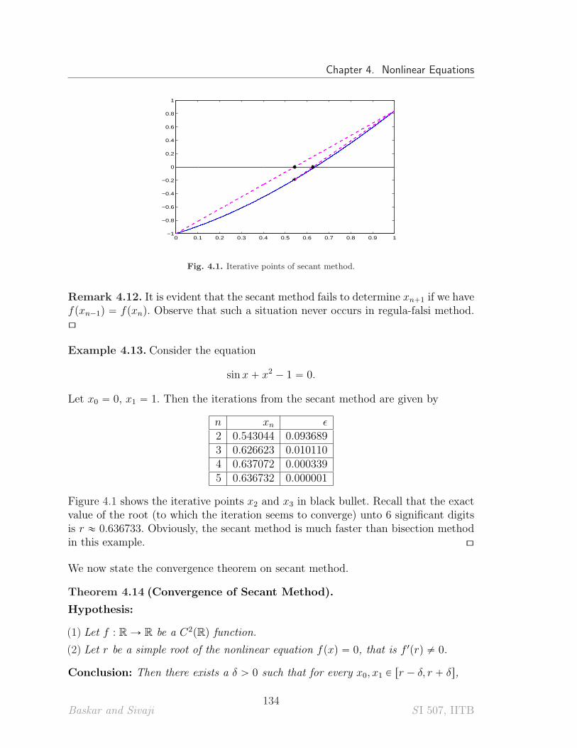
Chapter 4. Nonlinear Equations
0 0.1 0.2 0.3 0.4 0.5 0.6 0.7 0.8 0.9 1−1
−0.8
−0.6
−0.4
−0.2
0
0.2
0.4
0.6
0.8
1
Fig. 4.1. Iterative points of secant method.
Remark 4.12. It is evident that the secant method fails to determine xn`1 if we havefpxn´1q “ fpxnq. Observe that such a situation never occurs in regula-falsi method.[\
Example 4.13. Consider the equation
sinx ` x2 ´ 1 “ 0.
Let x0 “ 0, x1 “ 1. Then the iterations from the secant method are given by
n xn ϵ2 0.543044 0.0936893 0.626623 0.0101104 0.637072 0.0003395 0.636732 0.000001
Figure 4.1 shows the iterative points x2 and x3 in black bullet. Recall that the exactvalue of the root (to which the iteration seems to converge) unto 6 significant digitsis r « 0.636733. Obviously, the secant method is much faster than bisection methodin this example. [\
We now state the convergence theorem on secant method.
Theorem 4.14 (Convergence of Secant Method).
Hypothesis:
(1) Let f : R Ñ R be a C2pRq function.
(2) Let r be a simple root of the nonlinear equation fpxq “ 0, that is f 1prq ‰ 0.
Conclusion: Then there exists a δ ą 0 such that for every x0, x1 P rr ´ δ, r ` δs,
Baskar and Sivaji134
S I 507, IITB
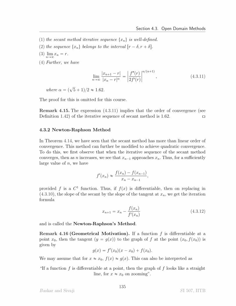
Section 4.3. Open Domain Methods
(1) the secant method iterative sequence txnu is well-defined.
(2) the sequence txnu belongs to the interval rr ´ δ, r ` δs.
(3) limnÑ8
xn “ r.
(4) Further, we have
limnÑ8
|xn`1 ´ r|
|xn ´ r|α“
ˇ
ˇ
ˇ
ˇ
f 2prq
2f 1prq
ˇ
ˇ
ˇ
ˇ
α{pα`1q
, (4.3.11)
where α “ p?5 ` 1q{2 « 1.62.
The proof for this is omitted for this course.
Remark 4.15. The expression (4.3.11) implies that the order of convergence (seeDefinition 1.42) of the iterative sequence of secant method is 1.62. [\
4.3.2 Newton-Raphson Method
In Theorem 4.14, we have seen that the secant method has more than linear order ofconvergence. This method can further be modified to achieve quadratic convergence.To do this, we first observe that when the iterative sequence of the secant methodconverges, then as n increases, we see that xn´1 approaches xn. Thus, for a sufficientlylarge value of n, we have
f 1pxnq «fpxnq ´ fpxn´1q
xn ´ xn´1
,
provided f is a C1 function. Thus, if fpxq is differentiable, then on replacing in(4.3.10), the slope of the secant by the slope of the tangent at xn, we get the iterationformula
xn`1 “ xn ´fpxnq
f 1pxnq(4.3.12)
and is called the Newton-Raphson’s Method.
Remark 4.16 (Geometrical Motivation). If a function f is differentiable at apoint x0, then the tangent (y “ gpxq) to the graph of f at the point px0, fpx0qq isgiven by
gpxq “ f 1px0qpx ´ x0q ` fpx0q.
We may assume that for x « x0, fpxq « gpxq. This can also be interpreted as
“If a function f is differentiable at a point, then the graph of f looks like a straightline, for x « x0 on zooming”.
Baskar and Sivaji135
S I 507, IITB
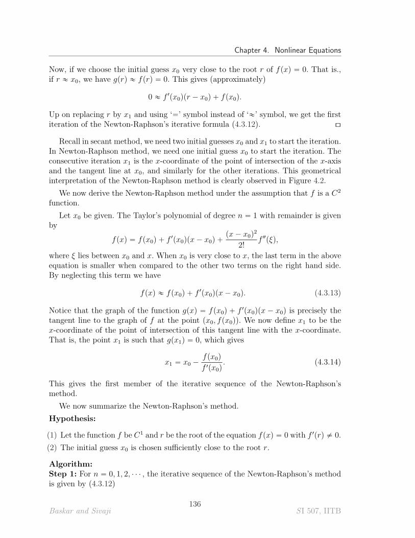
Chapter 4. Nonlinear Equations
Now, if we choose the initial guess x0 very close to the root r of fpxq “ 0. That is.,if r « x0, we have gprq « fprq “ 0. This gives (approximately)
0 « f 1px0qpr ´ x0q ` fpx0q.
Up on replacing r by x1 and using ‘“’ symbol instead of ‘«’ symbol, we get the firstiteration of the Newton-Raphson’s iterative formula (4.3.12). [\
Recall in secant method, we need two initial guesses x0 and x1 to start the iteration.In Newton-Raphson method, we need one initial guess x0 to start the iteration. Theconsecutive iteration x1 is the x-coordinate of the point of intersection of the x-axisand the tangent line at x0, and similarly for the other iterations. This geometricalinterpretation of the Newton-Raphson method is clearly observed in Figure 4.2.
We now derive the Newton-Raphson method under the assumption that f is a C2
function.
Let x0 be given. The Taylor’s polynomial of degree n “ 1 with remainder is givenby
fpxq “ fpx0q ` f 1px0qpx ´ x0q `px ´ x0q
2
2!f2pξq,
where ξ lies between x0 and x. When x0 is very close to x, the last term in the aboveequation is smaller when compared to the other two terms on the right hand side.By neglecting this term we have
fpxq « fpx0q ` f 1px0qpx ´ x0q. (4.3.13)
Notice that the graph of the function gpxq “ fpx0q ` f 1px0qpx ´ x0q is precisely thetangent line to the graph of f at the point px0, fpx0qq. We now define x1 to be thex-coordinate of the point of intersection of this tangent line with the x-coordinate.That is, the point x1 is such that gpx1q “ 0, which gives
x1 “ x0 ´fpx0q
f 1px0q. (4.3.14)
This gives the first member of the iterative sequence of the Newton-Raphson’smethod.
We now summarize the Newton-Raphson’s method.
Hypothesis:
(1) Let the function f be C1 and r be the root of the equation fpxq “ 0 with f 1prq ‰ 0.
(2) The initial guess x0 is chosen sufficiently close to the root r.
Algorithm:Step 1: For n “ 0, 1, 2, ¨ ¨ ¨ , the iterative sequence of the Newton-Raphson’s methodis given by (4.3.12)
Baskar and Sivaji136
S I 507, IITB
Section 4.3. Open Domain Methods
0 0.1 0.2 0.3 0.4 0.5 0.6 0.7 0.8 0.9 1−2
−1.5
−1
−0.5
0
0.5
1
Fig. 4.2. Iteration Procedure of Newton-Raphson’s method for fpxq “ sinpxq ` x2 ´ 1.
xn`1 “ xn ´fpxnq
f 1pxnq.
Step 2: Choose any one of the stopping criteria (or a combination of them) discussedin Section 4.2. If this criterion is satisfied, stop the iteration. Otherwise, repeat thestep 1 until the criterion is satisfied. [\
Remark 4.17. It is evident that if the initial guess x0 is such that f 1pxnq “ 0, forsome n P N, then the Newton-Raphson method fails. Geometrically, this means thatthe tangent line to the graph of f at the point pxn, fpxnqq is parallel to the x-axis.Therefore, this line never intersects x-axis and hence xn`1 never exists. See Remark4.12 for the failure of secant method and compare it with the present case. [\
Example 4.18. Consider the equation
sin x ` x2 ´ 1 “ 0.
Let x0 “ 1. Then the iterations from the Newton-Raphson method gives
n xn ϵ1 0.668752 0.0320192 0.637068 0.0003353 0.636733 0.000000
Figure 4.2 shows the iterative points x2 and x3 in black bullet. Recall that the exactsolution is x˚ « 0.636733. Obviously, the Newton-Raphson method is much fasterthan both bisection and secant methods in this example. [\
Let us now discuss the convergence of the Newton-Raphson method.
Baskar and Sivaji137
S I 507, IITB
Chapter 4. Nonlinear Equations
Theorem 4.19 (Error Estimates and Convergence of Newton-Raphson method).
Hypothesis:
(1) Let f : R Ñ R be a C2pRq function.
(2) Let r be a simple root of the nonlinear equation fpxq “ 0, that is f 1prq ‰ 0.
Conclusion: Then there exists a δ ą 0 such that for every x0 P rr ´ δ, r ` δs,
(1) each term of the Newton-Raphson iterative sequence txnu is well-defined.
(2) the sequence txnu belongs to the interval rr ´ δ, r ` δs.
(3) limnÑ8 xn “ r.
Proof: The Newton-Raphson sequence is defined by
xn`1 “ xn ´fpxnq
f 1pxnq.
The error en`1 :“ r ´ xn`1 can be written as
en`1 “pr ´ xnqf 1pxnq ` fpxnq
f 1pxnq
Using Taylor’s theorem, we have
0 “ fprq “ fpxnq ` pr ´ xnqf 1pxnq `f 2pξnq
2pr ´ xnq2, (4.3.15)
where ξn lies between r and xn. Using the information from the last equation, we getthe following expression for en`1:
en`1 “ ´f 2pξnq
2f 1pxnqpr ´ xnq2 “ ´
f2pξnq
2f 1pxnqe2n. (4.3.16)
Since f 1prq ‰ 0, there exists a δ1 ą 0 such that f 1pxq ‰ 0 for every x P rr´ δ1, r` δ1s.In particular, there exists Mδ1 ą 0 such that
minxPrr´δ1,r`δ1s
|f 1pxq| “ Mδ1 .
Also, since f 2 is a continuous function, there exists a Lδ1 ą 0 such that
maxxPrr´δ1,r`δ1s
|f2pxq| “ Lδ1 .
Thus we get
|en`1| ďLδ1
2Mδ1
|en|2. (4.3.17)
Baskar and Sivaji138
S I 507, IITB
Section 4.3. Open Domain Methods
Note that Cδ1 :“Lδ1
2Mδ1is a non-decreasing function of δ1, which implies that Cδ1
remains bounded as we decrease the value of δ1. Thus, there exists a δ ă 1 such thatδ ă δ1, and δ Cδ ă 1. We will now show that this δ has the required property. Theinequality (4.3.17), for this δ reads
|en`1| ď Cδ|en|2. (4.3.18)
Proof of (1) and (2): Let x0 P rr ´ δ, r ` δs. In other words, |r ´ x0| ď δ. Then x1is well-defined as f 1px0q ‰ 0, since x0 belongs to the interval rr ´ δ, r ` δs on whichf 1 is never equal to zero. We will prove that |r ´ x1| ď δ.
|r ´ x1| “ |e1| ď Cδ|e0|2 ď Cδδ|e0| ď |e0| ď δ.
By induction, it follows that xn is well-defined, and |r ´ xn| ď δ for every n P N.
Proof of (3): From the inequalities,
|en`1| ď Cδ|en|2 ď δCδ|en| ď pδCδq2|en´1| ď ¨ ¨ ¨ ď pδCδq
n`1|e0|,
the convergence of the sequence follows as δ Cδ ă 1. [\
Theorem on Newton-Raphson method says that if we start near-by a root ofthe nonlinear equation, then Newton-Raphson iterative sequence is well-defined andconverges. For increasing convex functions, we need not be very careful in choosingthe initial guess. For such functions, the Newton-Raphson iterative sequence alwaysconverges, whatever may be the initial guess. This is the content of the next theorem.
Theorem 4.20 (Convergence Result for Convex Functions).
Hypothesis: Let f : R Ñ R be a twice continuously differentiable function such that
(1) f is convex, i.e., f 2pxq ą 0 for all x P R.(2) f is strictly increasing, i.e., f 1pxq ą 0 for all x P R.(3) there exists an r P R such that fprq “ 0.
Conclusion: Then
(1) r is the unique solution of fpxq “ 0.
(2) For every choice of x0, the Newton-Raphson iterative sequence converges to r.
Proof:Proof of (1): Since f is strictly increasing, the function cannot take the same valuemore than once. Thus fpxq “ 0 has exactly one solution.
Proof of (2): From (4.3.16), it follows that en`1 ď 0. This implies that r ď xn`1.Since f is a strictly increasing function, we get fprq ď fpxn`1q. Thus fpxn`1q ě 0
Baskar and Sivaji139
S I 507, IITB
Chapter 4. Nonlinear Equations
for every n P N. From (4.3.12), we get xn`1 ď xn. That is, the sequence txnu is anon-increasing sequence, and is bounded below by r, and hence converges. Let usdenote the limit by x˚.
On the other hand, the sequence tenu is a non-decreasing sequence, bounded aboveby 0. Let e˚ denote the limit of the sequence tenu.
Passing to the limit as n Ñ 8 in the equation
en`1 “ en `fpxnq
f 1pxnq,
we get
e˚ “ e˚ `fpx˚q
f 1px˚q.
From the last equality, we get fpx˚q “ 0. [\
Remark 4.21. It follows from (4.3.18) that the order of convergence of the Newton-Raphson method is 2 (see Definition 1.42(3)), that is the Newton-Raphson iterativesequence converges quadratically. [\
To following example illustrates the quadratic convergence of the Newton-Raphsonmethod.
Example 4.22. Start with x0 “ ´2.4 and use Newton-Raphson iteration to find theroot r “ ´2.0 of the polynomial
fpxq “ x3 ´ 3x ` 2.
The iteration formula is
xn`1 “2x3n ´ 2
3x2n ´ 3.
It is easy to verify that |r´xn`1|{|r´xn|2 « 2{3, which shows the quadratic conver-gence of Newton-Raphson’s method as proved in the above theorem. [\
4.3.3 Fixed-Point Iteration Method
In fixed point iteration method, search for a solution of nonlinear equation fpxq “ 0is replaced by search for a fixed point of a function g, and with the property that ifα P R is a fixed point of g (i.e., gpαq “ α), then fpαq “ 0.
In general, there may be more than one choice of g with this property as illustratedby the following example.
Example 4.23. Note that α P R is a solution of the equation x2 ´ x ´ 2 “ 0 if andonly if α is a solution of each of the following equations.
Baskar and Sivaji140
S I 507, IITB
Section 4.3. Open Domain Methods
(1) x “ x2 ´ 2
(2) x “?x ` 2
(3) x “ 1 `2
x.
The fixed-point iteration method for finding a solution of gpxq “ x consists ofa sequence of iterates txnu, starting from an initial guess x0, defined by
xn “ gpxn´1q (4.3.19)
As we saw in Example 4.23, for a given nonlinear equation, the iteration function isnot unique. The crucial point in this method is to choose a good iteration functiongpxq. A good iteration function should satisfy the following properties:
(1) For the given starting point x0, the successive approximations xn given by (4.3.19)can be calculated.
(2) The sequence x1, x2, ¨ ¨ ¨ converges to some point ξ.
(3) The limit ξ is a fixed point of gpxq, ie., ξ “ gpξq.
Not every iteration function has all these properties. The following example showsthat for certain iteration functions, even the sequence of iterates need not be defined.
Example 4.24. Consider the equation
x2 ´ x “ 0.
This equation can be re-written as x “ ˘?x. Let us take the iterative function
gpxq “ ´?x.
Since gpxq is defined only for x ą 0, we have to choose x0 ą 0. For this value of x0,we have gpx0q ă 0 and therefore, x1 cannot be calculated. [\
Therefore, the choice of gpxq has to be made carefully so that the sequence of iteratescan be calculated.
How to choose such an iteration function gpxq?
Note that x1 “ gpx0q, and x2 “ gpx1q. Thus x1 is defined whenever x0 belongs tothe domain of g. Thus we must take the initial guess x0 from the domain of g. Fordefining x2, we need that x1 is in the domain of g once again. In fact the sequence isgiven by
x0, gpx0q, g ˝ gpx0q, g ˝ g ˝ gpx0q, ¨ ¨ ¨
Thus to have a well-defined iterative sequence, we require that
Range of the function g is contained in the domain of g.
Baskar and Sivaji141
S I 507, IITB
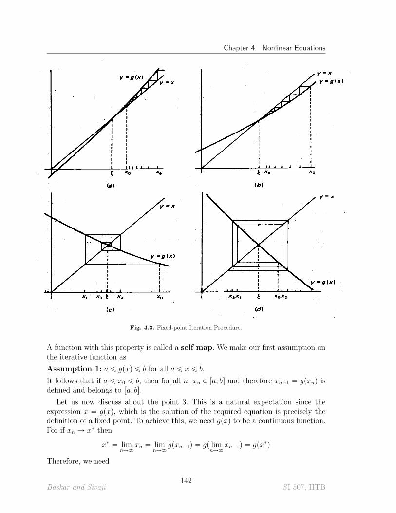
Chapter 4. Nonlinear Equations
Fig. 4.3. Fixed-point Iteration Procedure.
A function with this property is called a self map. We make our first assumption onthe iterative function as
Assumption 1: a ď gpxq ď b for all a ď x ď b.
It follows that if a ď x0 ď b, then for all n, xn P ra, bs and therefore xn`1 “ gpxnq isdefined and belongs to ra, bs.
Let us now discuss about the point 3. This is a natural expectation since theexpression x “ gpxq, which is the solution of the required equation is precisely thedefinition of a fixed point. To achieve this, we need gpxq to be a continuous function.For if xn Ñ x˚ then
x˚ “ limnÑ8
xn “ limnÑ8
gpxn´1q “ gp limnÑ8
xn´1q “ gpx˚q
Therefore, we need
Baskar and Sivaji142
S I 507, IITB
Section 4.3. Open Domain Methods
Assumption 2: The iterative function g is continuous.
It is easy to prove that a continuous self map on a bounded interval always hasa fixed point. However, the question is whether the sequence (4.3.19) generated bythe iterative function g converges, which is the requirement stated in point 2. Thispoint is well understood geometrically. The Figures 4.3(a) and 4.3(c) illustrate theconvergence of the fixed-point iterations whereas the Figures 4.3(b) and 4.3(d) il-lustrate the diverging iterations. In this geometrical observation, we see that wheng1pxq ă 1, we have convergence and otherwise, we have divergence. Therefore, wemake the assumption
Assumption 3: The iteration function gpxq is differentiable on I “ ra, bs. Further,there exists a constant 0 ă K ă 1 such that
|g1pxq| ď K, x P I. (4.3.20)
Such a function is called the contraction map.
Let us now present the algorithm of the fixed point iteration method.
Hypothesis: Assumptions 1, 2, and 3 stated above.
Algorithm: Choose an appropriate iteration function g : ra, bs Ñ ra, bs, where theinterval ra, bs is chosen in such a way that g is a self map.
Step 1: Choose an initial guess x0 P ra, bs.
Step 2: Define the iteration methods as
xn`1 “ gpxnq, n “ 0, 1, ¨ ¨ ¨
Step 3: For a pre-assigned positive quantity ϵ, check for one of the (fixed) stop-ping criteria discussed in Section 4.2. If the criterion is satisfied, stop the iteration.Otherwise, repeat the step 1 until the criterion is satisfied. [\
Theorem 4.25 (Convergence Result for Fixed-Point Iteration Method).
Hypothesis: Let the iterative function g be chosen so that
(1) g is defined on the interval ra, bs and a ď gpxq ď b. That is, g is a self map onra, bs
(2) g is continuously differentiable on ra, bs
(3) g is a contraction map. That is,
λ “ maxaďxďb
|g1pxq| ă 1. (4.3.21)
Conclusion: Then
(1) x “ gpxq has a unique solution r in ra, bs.
Baskar and Sivaji143
S I 507, IITB
Chapter 4. Nonlinear Equations
(2) For any choice of x0 P ra, bs, with xn`1 “ gpxnq, n “ 0, 1, ¨ ¨ ¨ ,
limnÑ8
xn “ r.
(3) We further have
|xn ´ r| ď λn|x0 ´ r| ďλn
1 ´ λ|x1 ´ x0| (4.3.22)
and
limnÑ8
r ´ xn`1
r ´ xn“ g1prq. (4.3.23)
Proof. Proof for (1) is easy.
From mean-value theorem and (4.3.20), we have
|r ´ xn`1| “ |gprq ´ gpxnq| ď λ|r ´ xn|. (4.3.24)
By induction, we have
|r ´ xn`1| ď λn|x0 ´ r|, n “ 0, 1, ¨ ¨ ¨ .
Since, as n Ñ 8, λn Ñ 0, we have xn Ñ r. Further, we have
|x0 ´ r| “ |x0 ´ x1 ` x1 ´ r|
ď |x0 ´ x1| ` |x1 ´ r|
ď λ|x0 ´ r| ` |x0 ´ x1|.
Then solving for |x0 ´ r|, we get (4.3.22).
Now we will prove the rate of convergence (4.3.23). From Mean-value theorem
r ´ xn`1 “ gprq ´ gpxnq “ g1pξnqpr ´ xnq, n “ 0, 1, ¨ ¨ ¨ .
with ξn an unknown point between r and xn. Since xn Ñ r, we must have ξn Ñ rand therefore,
limnÑ8
r ´ xn`1
r ´ xn“ lim
nÑ8g1pξnq “ g1prq.
This completes the proof. [\
Remark 4.26. From the inequality (4.3.24), we see that the fixed point iterationmethod has linear convergence. In other words, the order of convergence of thismethod is 1. [\
Baskar and Sivaji144
S I 507, IITB
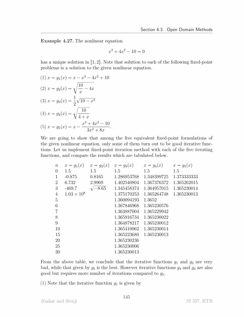
Section 4.3. Open Domain Methods
Example 4.27. The nonlinear equation
x3 ` 4x2 ´ 10 “ 0
has a unique solution in r1, 2s. Note that solution to each of the following fixed-pointproblems is a solution to the given nonlinear equation.
(1) x “ g1pxq “ x ´ x3 ´ 4x2 ` 10
(2) x “ g2pxq “
c
10
x´ 4x
(3) x “ g3pxq “1
2
?10 ´ x3
(4) x “ g4pxq “
c
10
4 ` x
(5) x “ g5pxq “ x ´x3 ` 4x2 ´ 10
3x2 ` 8x.
We are going to show that among the five equivalent fixed-point formulations ofthe given nonlinear equation, only some of them turn out to be good iterative func-tions. Let us implement fixed-point iteration method with each of the five iteratingfunctions, and compare the results which are tabulated below.
n x “ g1pxq x “ g2pxq x “ g3pxq x “ g4pxq x “ g5pxq
0 1.5 1.5 1.5 1.5 1.51 -0.875 0.8165 1.286953768 1.348399725 1.3733333332 6.732 2.9969 1.402540804 1.367376372 1.3652620153 -469.7
?´8.65 1.345458374 1.364957015 1.365230014
4 1.03 ˆ 108 1.375170253 1.365264748 1.3652300135 1.360094193 1.36526 1.367846968 1.3652305767 1.363887004 1.3652299428 1.365916734 1.3652300229 1.364878217 1.36523001210 1.365410062 1.36523001415 1.365223680 1.36523001320 1.36523023625 1.36523000630 1.365230013
From the above table, we conclude that the iterative functions g1 and g2 are verybad, while that given by g5 is the best. However iterative functions g3 and g4 are alsogood but requires more number of iterations compared to g5.
(1) Note that the iterative function g1 is given by
Baskar and Sivaji145
S I 507, IITB
Chapter 4. Nonlinear Equations
g1pxq “ x ´ x3 ´ 4x2 ` 10.
Note that g1p1q “ 6 and g1p2q “ ´12. Thus range of g1 is not contained in r1, 2s.That is g1 is not a self map on the interval r1, 2s. In fact,
g11pxq “ 1 ´ 3x2 ´ 8x.
Let us compute the minimum and maximum values of g11 on the interval r1, 2s. Note
that g21pxq “ ´6x ´ 8. Thus derivative of g1
1 vanishes at only one point, namelyx “ ´4
3which is not in the interval r1, 2s. Thus g1
1 has no maxima/minima in theinterval p1, 2q. Hence maximum and minimum of g1
1 are at the points 1, 2. Notethat g1
1p1q “ ´10, g11p2q “ ´27. Thus |g1pxq| ě 10 on the interval r1, 2s. Thus the
map g1 is not only not contractive on r1, 2s but is an expansive map on r1, 2s. Thisis the reason why the successive iterates using g1 have increasing moduli.
(2) Note that the iterative function g2 is given by
g2pxq “
c
10
x´ 4x.
It is easy to check that g2 is not a self map of r1, 2s to itself. In our computationabove, we see that the entire iterative sequence is not defined as one of the iteratesbecomes negative, when the initial guess is taken as 1.5 The exact solution isapproximately equal to x˚ “ 1.365 There is no interval containing x˚ on which|g1
2pxq| ă 1. In fact, g12px
˚q « 3.4 and as a consequence |g12pxq| ą 3 on an interval
containing x˚. Thus we dont expect a convergent iterative sequence even if thesequence is well-defined!
(3) Note that the iterative function g3 is given by
g3pxq “1
2
?10 ´ x3.
Note that g3 is a decreasing function on r1, 2s as
g13pxq “ ´
3x2
4?10 ´ x3
ă 0
on r1, 2s. Thus maximum of g3 is attained at x “ 1, which is 1.5; and the minimumis attained at x “ 2 which is approximately equal to 0.707. Thus g3 is a self mapof r1, 2s. But |g1
3p2q| « 2.12. Thus the condition
|g13pxq| ď λ ă 1
is violated on the interval r1, 2s. However by restricting to a smaller intervalr1, 1.5s, we get that g3 is a self map of r1, 1.5s as g3 is still decreasing function onr1, 1.5s and g3p1q “ 1.5, g3p1.5q « 1.28, and also
|g13pxq| ď |g1
3p1.5q| « 0.66.
Thus g3 satisfies the hypothesis of theorem on fixed-point iteration, and as ex-pected the sequence of iterates converge.
Baskar and Sivaji146
S I 507, IITB
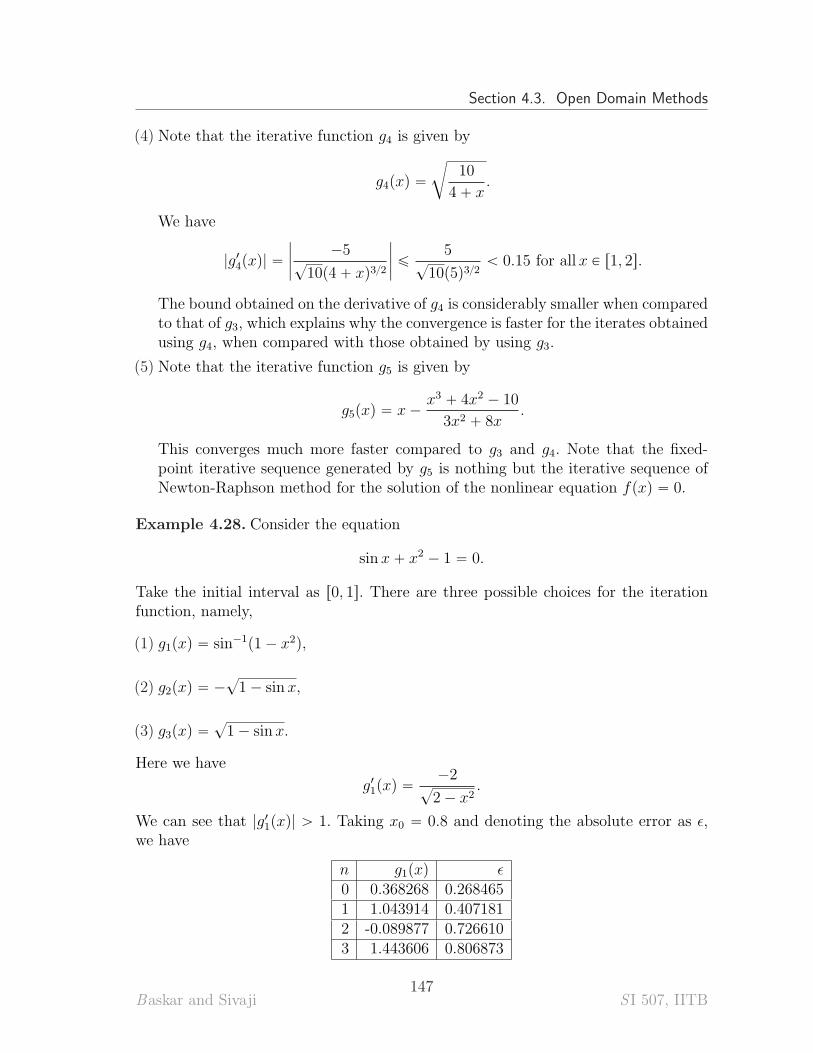
Section 4.3. Open Domain Methods
(4) Note that the iterative function g4 is given by
g4pxq “
c
10
4 ` x.
We have
|g14pxq| “
ˇ
ˇ
ˇ
ˇ
´5?10p4 ` xq3{2
ˇ
ˇ
ˇ
ˇ
ď5
?10p5q3{2
ă 0.15 for all x P r1, 2s.
The bound obtained on the derivative of g4 is considerably smaller when comparedto that of g3, which explains why the convergence is faster for the iterates obtainedusing g4, when compared with those obtained by using g3.
(5) Note that the iterative function g5 is given by
g5pxq “ x ´x3 ` 4x2 ´ 10
3x2 ` 8x.
This converges much more faster compared to g3 and g4. Note that the fixed-point iterative sequence generated by g5 is nothing but the iterative sequence ofNewton-Raphson method for the solution of the nonlinear equation fpxq “ 0.
Example 4.28. Consider the equation
sin x ` x2 ´ 1 “ 0.
Take the initial interval as r0, 1s. There are three possible choices for the iterationfunction, namely,
(1) g1pxq “ sin´1p1 ´ x2q,
(2) g2pxq “ ´?1 ´ sin x,
(3) g3pxq “?1 ´ sin x.
Here we have
g11pxq “
´2?2 ´ x2
.
We can see that |g11pxq| ą 1. Taking x0 “ 0.8 and denoting the absolute error as ϵ,
we have
n g1pxq ϵ0 0.368268 0.2684651 1.043914 0.4071812 -0.089877 0.7266103 1.443606 0.806873
Baskar and Sivaji147
S I 507, IITB
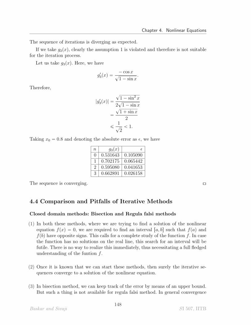
Chapter 4. Nonlinear Equations
The sequence of iterations is diverging as expected.
If we take g2pxq, clearly the assumption 1 is violated and therefore is not suitablefor the iteration process.
Let us take g3pxq. Here, we have
g13pxq “
´ cos x?1 ´ sinx
.
Therefore,
|g13pxq| “
?1 ´ sin2 x
2?1 ´ sinx
“
?1 ` sinx
2
ď1
?2
ă 1.
Taking x0 “ 0.8 and denoting the absolute error as ϵ, we have
n g3pxq ϵ0 0.531643 0.1050901 0.702175 0.0654422 0.595080 0.0416533 0.662891 0.026158
The sequence is converging. [\
4.4 Comparison and Pitfalls of Iterative Methods
Closed domain methods: Bisection and Regula falsi methods
(1) In both these methods, where we are trying to find a solution of the nonlinearequation fpxq “ 0, we are required to find an interval ra, bs such that fpaq andfpbq have opposite signs. This calls for a complete study of the function f . In casethe function has no solutions on the real line, this search for an interval will befutile. There is no way to realize this immediately, thus necessitating a full fledgedunderstanding of the funtion f .
(2) Once it is known that we can start these methods, then surely the iterative se-quences converge to a solution of the nonlinear equation.
(3) In bisection method, we can keep track of the error by means of an upper bound.But such a thing is not available for regula falsi method. In general convergence
Baskar and Sivaji148
S I 507, IITB
Section 4.4. Comparison and Pitfalls of Iterative Methods
of bisection method iterates is slower compared to that of regula falsi methoditerates.
(4) If the initial interval ra, bs is such that the equation fpxq “ 0 has a unique solutionin it, then both the methods converge to the solution. If there are more than onesolutions in ra, bs, then usually both methods find different solutions. The onlyway of finding the desired root is to find an interval in which there is exactly onesolution to the nonlinear equation.
Open domain methods: Secant, Newton-Raphson, and Fixed point meth-ods
(1) The main advantage of the open domain methods when compared to closed do-main methods is that we don’t need to locate a root in an interval. Rather, wecan start the iteration with an arbitrarily chosen initial guess(es).
(2) The disadvantage of the open domain methods is that the iterative sequence maynot be well-defined for all initial guesses. Even if the sequence is well-defined, itmay not converge. Even if it converges, it may not converge to a specific root ofinterest.
(3) In situations where both open and closed domain methods converge, open do-main methods are generally faster compared to closed domain methods. Espe-cially, Newton-Raphson’s method is faster than other methods as the order ofconvergence of this method is 2. In fact, this is the fastest method known today.
(4) In these methods, it may happen that we are trying to find a particular solutionof the nonlinear equation, but the iterative sequence may converge to a differentsolution. Thus we have to be careful in choosing the initial guess. If the initialguess is far away from the expected root, then there is a danger that the iterationconverges to another root of the equation.
In the case of Newton-Raphson’s method, this usually happens when the slopef 1px0q is small and the tangent line to the curve y “ fpxq is nearly parallel tothe x-axis. Similarly, in the case of secant method, this usually happens whenthe slope of the secant joining px0, fpx0qq and px1, fpx1qq is nearly parallel to thex-axis.
For example, iffpxq “ cos x
and we seek the root x˚ “ π{2 and start with x0 “ 3, calculation reveals that
x1 “ ´4.01525, x2 “ ´4.85266, ¨ ¨ ¨ ,
Baskar and Sivaji149
S I 507, IITB
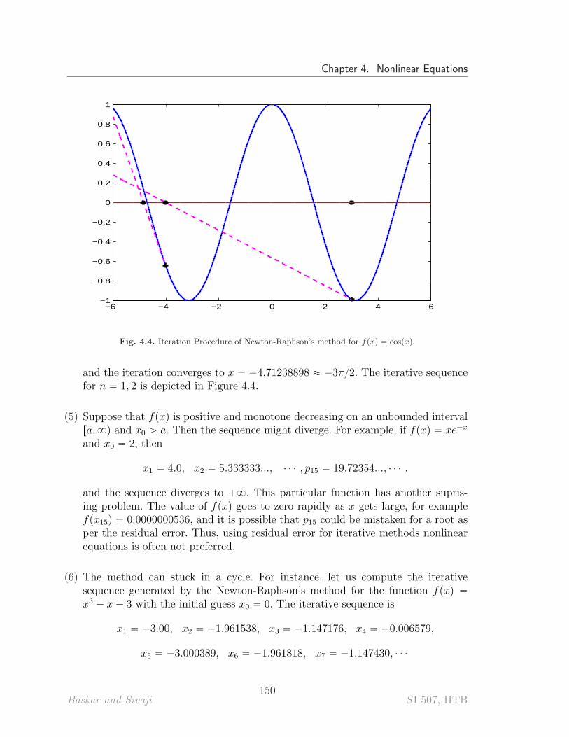
Chapter 4. Nonlinear Equations
−6 −4 −2 0 2 4 6−1
−0.8
−0.6
−0.4
−0.2
0
0.2
0.4
0.6
0.8
1
Fig. 4.4. Iteration Procedure of Newton-Raphson’s method for fpxq “ cospxq.
and the iteration converges to x “ ´4.71238898 « ´3π{2. The iterative sequencefor n “ 1, 2 is depicted in Figure 4.4.
(5) Suppose that fpxq is positive and monotone decreasing on an unbounded intervalra,8q and x0 ą a. Then the sequence might diverge. For example, if fpxq “ xe´x
and x0 “ 2, then
x1 “ 4.0, x2 “ 5.333333..., ¨ ¨ ¨ , p15 “ 19.72354..., ¨ ¨ ¨ .
and the sequence diverges to `8. This particular function has another supris-ing problem. The value of fpxq goes to zero rapidly as x gets large, for examplefpx15q “ 0.0000000536, and it is possible that p15 could be mistaken for a root asper the residual error. Thus, using residual error for iterative methods nonlinearequations is often not preferred.
(6) The method can stuck in a cycle. For instance, let us compute the iterativesequence generated by the Newton-Raphson’s method for the function fpxq “
x3 ´ x ´ 3 with the initial guess x0 “ 0. The iterative sequence is
x1 “ ´3.00, x2 “ ´1.961538, x3 “ ´1.147176, x4 “ ´0.006579,
x5 “ ´3.000389, x6 “ ´1.961818, x7 “ ´1.147430, ¨ ¨ ¨
Baskar and Sivaji150
S I 507, IITB
Section 4.5. Exercises
and we are stuck in a cycle where xn`4 « xk for k “ 0, 1, ¨ ¨ ¨ . But if we startwith a value x0 sufficiently close with the root r « 1.6717, then the convergenceis obtained. The proof of this is left as an exercise.
(7) If fpxq has no real root, then there is no indication by these methods and the iter-ative sequence may simply oscillate. For example compute the Newton-Raphsoniteration for
fpxq “ x2 ´ 4x ` 5.
4.5 Exercises
Bisection Method and Regula-falsi Method
In the following problems on bisection method, the notation xn is used to denotethe mid-point of the interval ran´1, bn´1s, and is termed as the bisection method’s nth
iterate (or simply, the nth iterate, as the context of bisection method is clear)
(1) Let bisection method be used to solve the nonlinear equation
2x6 ´ 5x4 ` 2 “ 0
starting with the initial interval r0, 1s. In order to approximate a solution of thenonlinear equation with an absolute error less than or equal to 10´3, what is theminimum number of iterations required? Also find the corresponding approximatesolution.
(2) Let bisection method be used to solve the nonlinear equation (x is in radians)
x sinx ´ 1 “ 0
starting with the initial interval r0, 2s. In order to approximate a solution of thenonlinear equation with an absolute error less than or equal to 10´3, what is theminimum number of iterations required? Also find the corresponding approximatesolution.
(3) Let bisection method be used to solve a nonlinear equation fpxq “ 0 starting withthe initial interval ra0, b0s where a0 ą 0. Let xn be as in the bisection method, andr be the solution of the nonlinear equation fpxq “ 0 to which bisection methodconverges. Let ϵ ą 0. Show that the relative error of xn w.r.t. r is at most ϵwhenever n satisfies
n ělogpb0 ´ a0q ´ log ϵ ´ log a0
log 2.
What happens if a0 ă 0 ă b0?
Baskar and Sivaji151
S I 507, IITB
Chapter 4. Nonlinear Equations
(4) Consider the nonlinear equation
10x ` x ´ 4 “ 0
(i) Find an interval ra0, b0s such that the function fpxq “ 10x ` x´ 4 satisfies thehypothesis of bisection method.
(ii) Let r be the solution of the nonlinear equation to which bisection method iter-ative sequence converges. Find an n such that xn (notation as in the bisectionmethod) approximates r to two significant digits. Also find xn.
(5) If bisection method is used with the initial interval ra0, b0s “ r2, 3s, how manyiterations are required to assure that an approximate solution of the nonlinearequation fpxq “ 0 is obtained with an absolute error that is at most 10´5?
(6) Assume that in solving a nonlinear equation fpxq “ 0 with the initial intervalra0, b0s, the iterative sequence txnu given by bisection method is never an exactsolution of fpxq “ 0. Let us define a sequence of numbers tdnu by
dn “
#
0 if ran, bns is the left half of the interval ran´1, bn´1s,
1 if ran, bns is the right half of the interval ran´1, bn´1s.
Using the sequence tdnu defined above, express the solution of fpxq “ 0 to whichthe bisection method converges. (Hint: Try the case ra0, b0s “ r0, 1s first andthink of binary representation of a number. Then try for the case ra0, b0s “ r0, 2s,then for the case ra0, b0s “ r1, 3s, and then the general case!)
(7) In the notation of bisection method, determine (with justification) if the followingare possible.
(i) a0 ă a1 ă a2 ă ¨ ¨ ¨ ă an ă ¨ ¨ ¨
(ii) b0 ą b1 ą b2 ą ¨ ¨ ¨ ą bn ą ¨ ¨ ¨
(iii) a0 “ a1 ă a2 “ a3 ă ¨ ¨ ¨ ă a2m “ a2m`1 ă ¨ ¨ ¨ (Hint: First guess what shouldbe the solution found by bisection method in such a case, and then find thesimplest function having it as a root! Do not forget the connection betweenbisection method and binary representation of a number, described in the lastproblem)
(8) Draw the graph of a function that satisfies the hypothesis of bisection method onthe interval r0, 1s such that the errors e1, e2, e3 satisfy e1 ą e2, and e2 ă e3. Giveformula for one such function.
(9) Draw the graph of a function for which bisection method iterates satisfy x1 “ 2,x2 “ 0, and x3 “ 1 (in the usual notation of bisection method). Indicate in thegraph why x1 “ 2, x2 “ 0, and x3 “ 1 hold. Also mention precisely the corre-sponding intervals ra0, b0s,ra1, b1s, ra2, b2s.
Baskar and Sivaji152
S I 507, IITB
Section 4.5. Exercises
(10) Draw the graph of a function (there is no need to give a formula for the func-tion) for which a0, a1, a2, a3 (in the usual notation of bisection method) satisfya0 ă a1 “ a2 ă a3. (Mark these points clearly on the graph.)
Secant Method and Newton-Raphson Method
(11) Discuss some instances where the secant method fails. Note that failure of secantmethod results from one of the following two situations: (i) the iterative sequenceis not well-defined, and (ii) the iterative sequence does not converge at all.
(12) Let α be a positive real number. Find formula for an iterative sequence based onNewton-Raphson method for finding
?α and α1{3. Apply the methods to α “ 18
to obtain the results whcih are correct to two significant digits when compared totheir exact values.
(13) Consider the nonlinear equation
1
3x3 ´ x2 ` x ` 1 “ 0.
Show that there exists an initial guess x0 P p0, 4q for which x2 of the Newton-Raphson method iterative sequence is not defined.
(14) Let a be a real number such that 0 ă a ď 1. Let txnu8n“1 be the iterative sequence
of the Newton-Raphson method to solve the nonlinear equation e´ax “ x. If x˚
denotes the exact root of this equation and x0 ą 0, then show that
|x˚ ´ xn`1| ď1
2px˚ ´ xnq2.
(15) Newton-Raphson method is to be applied for approximating a root of the nonlinearequation x4 ´ x ´ 10 “ 0.
(i) How many solutions of the nonlinear equation are there in r1,8q? Are theysimple?
(ii) Find an interval r1, bs that contains the smallest positive solution of the non-linear equation.
(iii) Compute five iterates of Newton-Raphson method, for each of the initialguesses x0 “ 1, x0 “ 2, x0 “ 100. What are your observations?
(iv) A solution of the nonlinear equation is approximately equal to 1.85558 Finda δ as in the proof of theorem on Newton-Raphson method, so that iterativesequence of Newton-Raphson method always converges for every initial guessx0 P r1.85558 ´ δ, 1.85558 ` δs.
(v) Can we appeal to the theorem for convex functions in the context of Newton-Raphson method? Justify.
Baskar and Sivaji153
S I 507, IITB
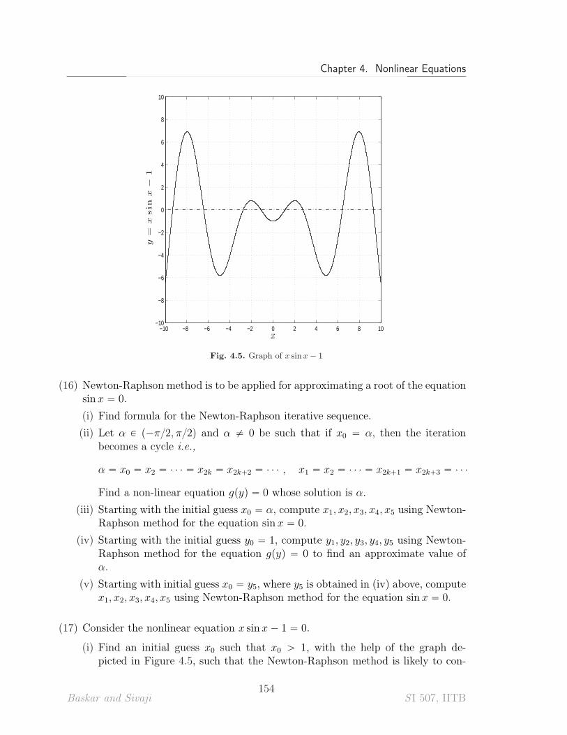
Chapter 4. Nonlinear Equations
−10 −8 −6 −4 −2 0 2 4 6 8 10−10
−8
−6
−4
−2
0
2
4
6
8
10
x
y=
xsinx−
1
Fig. 4.5. Graph of x sinx ´ 1
(16) Newton-Raphson method is to be applied for approximating a root of the equationsinx “ 0.
(i) Find formula for the Newton-Raphson iterative sequence.
(ii) Let α P p´π{2, π{2q and α ‰ 0 be such that if x0 “ α, then the iterationbecomes a cycle i.e.,
α “ x0 “ x2 “ ¨ ¨ ¨ “ x2k “ x2k`2 “ ¨ ¨ ¨ , x1 “ x2 “ ¨ ¨ ¨ “ x2k`1 “ x2k`3 “ ¨ ¨ ¨
Find a non-linear equation gpyq “ 0 whose solution is α.
(iii) Starting with the initial guess x0 “ α, compute x1, x2, x3, x4, x5 using Newton-Raphson method for the equation sinx “ 0.
(iv) Starting with the initial guess y0 “ 1, compute y1, y2, y3, y4, y5 using Newton-Raphson method for the equation gpyq “ 0 to find an approximate value ofα.
(v) Starting with initial guess x0 “ y5, where y5 is obtained in (iv) above, computex1, x2, x3, x4, x5 using Newton-Raphson method for the equation sinx “ 0.
(17) Consider the nonlinear equation x sinx ´ 1 “ 0.
(i) Find an initial guess x0 such that x0 ą 1, with the help of the graph de-picted in Figure 4.5, such that the Newton-Raphson method is likely to con-
Baskar and Sivaji154
S I 507, IITB

Section 4.5. Exercises
verge to the solution x˚ of the given nonlinear equation lying in the intervalp´10,´9q. Compute x1, x2, x3, x4 of the corresponding Newton-Raphson itera-tive sequence. Explain why the Newton-Raphson iterative sequence so obtainedwould converge to the desired x˚. This example shows that even though theinitial guess is close to a solution, the corresponding Newton-Raphson iterativesequence might converge to a solution that is far off!
(ii) Find another initial guess x0 such that x0 ą 1, with the help of the graph,such that the Newton-Raphson method is likely to converge to the smallestpositive solution of the given nonlinear equation. Compute x1, x2, x3, x4 of thecorresponding Newton-Raphson iterative sequence. Explain why the Newton-Raphson iterative sequence so obtained would converge to the desired solution.
(18) Draw the graph of a function for which the Newton-Raphson iterates satisfyx0 “ x2 “ x4 “ ¨ ¨ ¨ “ 0, and x1 “ x3 “ x5 “ ¨ ¨ ¨ “ 2. Indicate in the graphwhy this happens.
(19) Draw the graph of a function for which regula-falsi method iterates satisfy x0 “ 0,x1 “ 3, and x2 “ 1, x3 “ 2 (in the usual notation of regula-falsi method). Indicatein the graph why x2 “ 1, x3 “ 2 hold.
Fixed-Point Iteration Method
(20) The nonlinear equation fpxq “ x2 ´ 2x ´ 8 “ 0 has two solutions x “ ´2 andx “ 4. Consider the three fixed-point formulations
(i) x “8
x ´ 2,
(ii) x “?2x ` 8,
(iii) x “x2 ´ 8
2.
Carry out fixed-point iteration method with two initial guesses x0 “ ´1, x0 “ 3,and for all the three iteration functions. Discuss the convergence or divergence ofall the iterative sequences. Can you justify theoretically?
(21) To solve the nonlinear equation x ´ tanx “ 0 by fixed-point iteration method,the following fixed-point formulations may be considered.
(i) x “ tanx
(ii) x “ tan´1 x
Discuss about convergence of the fixed-point iterative sequences generated by thetwo formulations.
Baskar and Sivaji155
S I 507, IITB
Chapter 4. Nonlinear Equations
(22) To solve the nonlinear equation e´x ´ cos x “ 0 by fixed-point iteration method,the following fixed-point formulations may be considered.
(i) x “ ´ lnpcos xq
(ii) x “ cos´1pe´xq
Discuss about convergence of the fixed-point iterative sequences generated by thetwo formulations.
(23) Show that gpxq “ π ` 12sinpx{2q has a unique fixed point in r0, 2πs. Use fixed-
point iteration method with g as the iteration function and x0 “ 0 to find anapproximate solution for the equaton 1
2sinpx{2q ´ x ` π “ 0 with the stopping
criterion that the residual error is less than 10´4.
(24) Let α P R and β P R be the roots of x2 ` ax ` b “ 0, and such that |α| ą |β|.Let g and h be two iterating functions satisfying the hypothesis of the theorem onfixed-point method. Consider the iterative sequences txnu and tynu correspondingto two the iterating functions g and h given by
xn`1 “ ´axn ` b
xn, and yn`1 “ ´
b
yn ` a
respectively. Show that the iterative sequences txnu and tynu converge to α andβ respectively.
(25) Let txnu Ă ra, bs be a sequence generated by a fixed point iteration method witha continuously differentiable iteration function gpxq. If this sequence converges tox˚, then show that
|xn`1 ´ x˚| ďλ
1 ´ λ|xn`1 ´ xn|,
where λ :“ maxxPra,bs
|g1pxq|. (This estimate helps us to decide when to stop iterating
if we are using a stopping criterion based on the distance between successive iter-ates.)
(26) Explain why the sequence of iterates xn`1 “ 1 ´ 0.9x2n, with initial guess x0 “ 0,does not converge to any solution of the quadratic equation 0.9x2 ` x ´ 1 “ 0?[Hint: Observe what happens after 25 iterations]
(27) Let x˚ be the smallest positive root of the equation 20x3 ´ 20x2 ´ 25x ` 4 “ 0.The following question is concerning the fixed-point formulation of the nonlinearequation given by x “ gpxq, where gpxq “ x3 ´ x2 ´ x
4` 1
5.
(i) Show that x˚ P r0, 1s.
Baskar and Sivaji156
S I 507, IITB
Section 4.5. Exercises
(ii) Does the function g satisfy the hypothesis of theorem on fixed-point method? Ifyes, we know that x˚ is the only fixed point of g lying in the interval r0, 1s. In thenotation of fixed-point iteration method, find an n such that |x˚ ´xn| ă 10´3,when the initial guess x0 is equal to 0.
(28) Let f : ra, bs Ñ R be a function such that f 1 is continuous, fpaqfpbq ă 0, andthere exists an α ą 0 such that f 1pxq ě α ą 0.
(i) Show that fpxq “ 0 has exactly one solution in the interval ra, bs.
(ii) Show that with a suitable choice of the parameter λ, the solution of the non-linear equation fpxq “ 0 can be obtained by applying the fixed-point iterationmethod applied to the function F pxq “ x ` λfpxq.
(29) Let p ą 1 be a real number. Show that the following expression has a meaningand find its value.
x “
c
p `
b
p `?p ` ¨ ¨ ¨
Note that the last equation is interpreted as x “ limnÑ8 xn, where x1 “?p,
x2 “a
p `?p, ¨ ¨ ¨ . (Hint: Note that xn`1 “
?p ` xn, and show that the se-
quence txnu converges using the theorem on fixed-point method.)
(30) Draw the graph of a function having the following properties: (i) The functionhas exactly TWO fixed points. (ii) Give two choices of the initial guess x0 andy0 such that the corresponding sequences txnu and tynu have the properties thattxnu converges to one of the fixed points and the sequence tynu goes away anddiverges. Point out the first three terms of both the sequences on the graph.
Baskar and Sivaji157
S I 507, IITB

CHAPTER 5
Interpolation
Let a physical experiment be conducted and the outcome is recorded only at somefinite number of times. If we want to know the outcome at some intermediate timewhere the data is not available, then we may have to repeat the whole experimentonce again to get this data. In the mathematical language, suppose that the finiteset of values
tfpxiq : i “ 0, 1, ¨ ¨ ¨ , nu
of a function f at a given set of points
txi : i “ 0, 1, ¨ ¨ ¨ , nu
is known and we want to find the value of fpxq, where x P pxj, xkq, for some j “
1, 2, ¨ ¨ ¨ , n and k “ 1, 2, ¨ ¨ ¨ , n. One way of obtaining the value of fpxq is to computethis value directly from the expression of the function f . Often, we may not knowthe expression of the function explicitly and only the data
tpxi, yiq : i “ 0, 1, ¨ ¨ ¨ , nu
is known, where yi “ fpxiq. In terms of the physical experiments, repeating anexperiment will quite often be very expensive. Therefore, one would like to get atleast an approximate value of fpxq (in terms of experiment, an approximate value ofthe outcome at the desired time). This is achieved by first constructing a functionwhose value at xi coincides exactly with the value fpxiq for i “ 0, 1, ¨ ¨ ¨ , n and thenfinding the value of this constructed function at the desired points. Such a processis called interpolation and the constructed function is called the interpolatingfunction for the given data.
In certain circumstances, the function f may be known explicitly, but still toodifficult to perform certain operations like differentiation and integration. Thus, itis useful to restrict the class of interpolating functions to polynomials, where thedifferentiation and integration can be done more easily.
In Sectoin 5.1, we introduce the basic problem of polynomial interpolation andprove the existence and uniqueness of polynomial interpolating the given data. Thereare at least two ways to obtain the unique polynomial interpolating a given data,
Chapter 5. Interpolation
one is the Lagrange and another one is the Newton. In Section 5.1.2, we introduceLagrange form of interpolating polynomial. Section 5.1.3 introduces the notion ofdivided differences and Newton form of interpolating polynomial. The error analysisof the polynomial interpolation is studied in Section 5.3. In certain cases, the interpo-lating polynomial can differ significantly from the exact function. This is illustratedby Carl Runge and is called the Runge Phenomenon. In Section 5.3.4 we presentthe example due to Runge and state a few results on convergence of the interpolat-ing polynomials. The concept of piecewise polynomial interpolation and Splineinterpolation are discussed in Section 5.5.
5.1 Polynomial Interpolation
Polynomial interpolation is a concept of fitting a polynomial to a given data. Thus,to construct an interpolating polynomial, we first need a set of points at which thedata values are known.
Definition 5.1. Any collection of distinct real numbers x0, x1, ¨ ¨ ¨ , xn (not necessarilyin increasing order) is called nodes.
Definition 5.2 (Interpolating Polynomial). Let x0, x1, ¨ ¨ ¨ , xn be the given nodesand y0, y1, ¨ ¨ ¨ , yn be real numbers. A polynomial pnpxq of degree less than or equal ton is said to be a polynomial interpolating the given data or an interpolatingpolynomial for the given data if
pnpxiq “ yi, i “ 0, 1, ¨ ¨ ¨n. (5.1.1)
The condition (5.1.1) is called the interpolation condition. [\
Remark 5.3. Let x0, x1, ¨ ¨ ¨ , xn be given nodes, and y0, y1, ¨ ¨ ¨ , yn be real numbers.Let pnpxq be a polynomial interpolating the given data. Then the graph of pnpxq
passes through the set of pn ` 1q distinct points in the xy-plane given by the table
x x0 x1 x2 x3 ¨ ¨ ¨ xny y0 y1 y2 y3 ¨ ¨ ¨ yn
.
We call the set tpxi, yiq, i “ 0, 1, ¨ ¨ ¨ , nu as data and quite often we represent this setin the above form of a table. [\
5.1.1 Existence and Uniqueness of Interpolating Polynomial
The following result asserts that an interpolating polynomial exists and is unique.
Theorem 5.4 (Existence and Uniqueness of Interpolating polynomial).
Let x0, x1, ¨ ¨ ¨ , xn be given nodes, and y0, y1, ¨ ¨ ¨ , yn be real numbers.
Baskar and Sivaji160
S I 507, IITB
Section 5.1. Polynomial Interpolation
(1) Then there exists a polynomial pnpxq of degree less than or equal to n such that
pnpxiq “ yi, i “ 0, 1, ¨ ¨ ¨ , n.
That is, pnpxq is an interpolating polynomial for the data tpxi, yiq, i “ 0, 1, ¨ ¨ ¨ , nu.
(2) Such a polynomial as above is unique.
Proof:Proof of uniqueness: Assume that pnpxq and qnpxq are interpolating polynomialsof degree less than or equal to n that satisfies the interpolation condition (5.1.1). Let
rnpxq “ pnpxq ´ qnpxq.
Then, rnpxq is also a polynomial of degree less than or equal to n, and by the inter-polation condition, we have
rnpxiq “ 0,
for every i “ 0, 1, ¨ ¨ ¨ , n. Thus, rnpxq is a polynomial of degree less than or equal to nwith n ` 1 distinct roots. By the fundamental theorem of algebra, we conclude thatrnpxq is the zero polynomial. That is, the interpolating polynomial is unique.
Proof of existence: Existence of interpolating polynomial is proved using mathe-matical induction. If n “ 0, then the constant polynomial
p0pxq “ y0
is the required polynomial and its degree is less than or equal to 0. Assume that theresult is true for n “ k. We will now prove that the result is true for n “ k ` 1.
Let the data be given by
x x0 x1 x2 x3 ¨ ¨ ¨ xk xk`1
y y0 y1 y2 y3 ¨ ¨ ¨ yk yk`1
By the assumption, there exists a polynomial pkpxq of degree less than or equal to ksuch that the first k interpolating conditions
pkpxiq “ yi, i “ 0, 1, ¨ ¨ ¨ , k
hold. Define a polynomial pk`1pxq of degree less than or equal to k ` 1 by
pk`1pxq “ pkpxq ` cpx ´ x0qpx ´ x1q ¨ ¨ ¨ px ´ xkq, (5.1.2)
where the constant c is such that the pk ` 1qth interpolation condition pk`1pxk`1q “
yk`1 holds. This is achieved by choosing
c “yk`1 ´ pkpxk`1q
pxk`1 ´ x0qpxk`1 ´ x1q ¨ ¨ ¨ pxk`1 ´ xkq.
Note that pk`1pxiq “ yi for i “ 0, 1, ¨ ¨ ¨ , k and therefore pk`1pxq is an interpolatingpolynomial for the given data. This proves the result for n “ k ` 1. By the principleof mathematical induction, the result is true for any natural number n. [\
Baskar and Sivaji161
S I 507, IITB
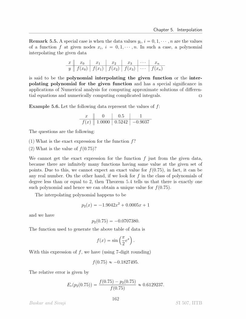
Chapter 5. Interpolation
Remark 5.5. A special case is when the data values yi, i “ 0, 1, ¨ ¨ ¨ , n are the valuesof a function f at given nodes xi, i “ 0, 1, ¨ ¨ ¨ , n. In such a case, a polynomialinterpolating the given data
x x0 x1 x2 x3 ¨ ¨ ¨ xny fpx0q fpx1q fpx2q fpx3q ¨ ¨ ¨ fpxnq
is said to be the polynomial interpolating the given function or the inter-polating polynomial for the given function and has a special significance inapplications of Numerical analysis for computing approximate solutions of differen-tial equations and numerically computing complicated integrals. [\
Example 5.6. Let the following data represent the values of f :
x 0 0.5 1fpxq 1.0000 0.5242 ´0.9037
The questions are the following:
(1) What is the exact expression for the function f?
(2) What is the value of fp0.75q?
We cannot get the exact expression for the function f just from the given data,because there are infinitely many functions having same value at the given set ofpoints. Due to this, we cannot expect an exact value for fp0.75q, in fact, it can beany real number. On the other hand, if we look for f in the class of polynomials ofdegree less than or equal to 2, then Theorem 5.4 tells us that there is exactly onesuch polynomial and hence we can obtain a unique value for fp0.75q.
The interpolating polynomial happens to be
p2pxq “ ´1.9042x2 ` 0.0005x ` 1
and we havep2p0.75q “ ´0.0707380.
The function used to generate the above table of data is
fpxq “ sin´π
2ex¯
.
With this expression of f , we have (using 7-digit rounding)
fp0.75q « ´0.1827495.
The relative error is given by
Erpp2p0.75qq “fp0.75q ´ p2p0.75q
fp0.75q« 0.6129237.
Baskar and Sivaji162
S I 507, IITB
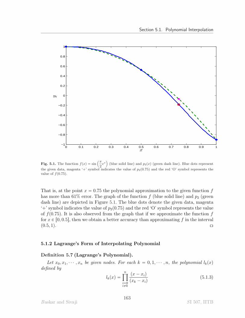
Section 5.1. Polynomial Interpolation
0 0.1 0.2 0.3 0.4 0.5 0.6 0.7 0.8 0.9 1−1
−0.8
−0.6
−0.4
−0.2
0
0.2
0.4
0.6
0.8
1
x
y
Fig. 5.1. The function fpxq “ sin´π
2ex¯
(blue solid line) and p2pxq (green dash line). Blue dots represent
the given data, magenta ‘+’ symbol indicates the value of p2p0.75q and the red ‘O’ symbol represents thevalue of fp0.75q.
That is, at the point x “ 0.75 the polynomial approximation to the given function fhas more than 61% error. The graph of the function f (blue solid line) and p2 (greendash line) are depicted in Figure 5.1. The blue dots denote the given data, magenta‘+’ symbol indicates the value of p2p0.75q and the red ‘O’ symbol represents the valueof fp0.75q. It is also observed from the graph that if we approximate the function ffor x P r0, 0.5s, then we obtain a better accuracy than approximating f in the intervalp0.5, 1q. [\
5.1.2 Lagrange’s Form of Interpolating Polynomial
Definition 5.7 (Lagrange’s Polynomial).
Let x0, x1, ¨ ¨ ¨ , xn be given nodes. For each k “ 0, 1, ¨ ¨ ¨ , n, the polynomial lkpxq
defined by
lkpxq “
nź
i“0i‰k
px ´ xiq
pxk ´ xiq(5.1.3)
Baskar and Sivaji163
S I 507, IITB
Chapter 5. Interpolation
is called the kth Lagrange Polynomial or the kth Lagrange Cardinal Function.
Remark 5.8. Note that the kth Lagrange polynomial depends on all the n` 1 nodesx0, x1, ¨ ¨ ¨ , xn. [\
Theorem 5.9 (Lagrange’s form of Interpolating Polynomial).
Hypothesis:
(1) Let x0, x1, ¨ ¨ ¨ , xn be given nodes.
(2) Let the values of a function f be given at these nodes.
(3) For each k “ 0, 1, ¨ ¨ ¨ , n, let lkpxq be the kth Lagrange polynomial.
(4) Let pnpxq (of degree ď n) be the polynomial interpolating the function f at thenodes x0, x1, ¨ ¨ ¨ , xn.
Conclusion: Then, pnpxq can be written as
pnpxq “
nÿ
i“0
fpxiqlipxq. (5.1.4)
This form of the interpolating polynomial is called the Lagrange’s form of Inter-polating Polynomial.
Proof: Firstly, we will prove that qpxq :“řn
i“0 fpxiqlipxq is an interpolating polyno-mial for the function f at the nodes x0, x1, ¨ ¨ ¨ , xn. Since
lipxjq “
#
1 if i “ j
0 if i ‰ j,
we get qpxjq “ fpxjq for each j “ 0, 1, ¨ ¨ ¨ , n. Thus, qpxq is an interpolating polyno-mial. Since interpolating polynomial is unique by Theorem 5.4, the polynomial qpxq
must be the same as pnpxq. This completes the proof of the theorem. [\
Example 5.10. Consider the case n “ 1 in which we have two distinct points x0 andx1. Then
l0pxq “x ´ x1x0 ´ x1
, l1pxq “x ´ x0x1 ´ x0
and
p1pxq “ fpx0ql0pxq ` fpx1ql1pxq
“ fpx0qx ´ x1x0 ´ x1
` fpx1qx ´ x0x1 ´ x0
“fpx0qpx ´ x1q ´ fpx1qpx ´ x0q
x0 ´ x1
“ fpx0q `fpx1q ´ fpx0q
x1 ´ x0px ´ x0q. (5.1.5)
Baskar and Sivaji164
S I 507, IITB
Section 5.1. Polynomial Interpolation
This is the linear interpolating polynomial of the function f . Similarly, if we aregiven three nodes with corresponding values, then we can generate the quadraticinterpolating polynomial and so on.. [\
Example 5.11. Let the values of the function fpxq “ ex be given at x0 “ 0.82 andx1 “ 0.83 by
e0.82 « 2.270500, e0.83 « 2.293319.
In this example, we would like to obtain an approximate value of e0.826 using thepolynomial p1pxq that interpolates f at the nodes x0, x1. The polynomial p1pxq isgiven by
p1pxq “ 2.270500 `2.293319 ´ 2.270500
0.83 ´ 0.82px ´ 0.82q “ 2.2819x ` 0.399342.
The approximate value of e0.826 is taken to be p1p0.826q, which is given by
p1p0.826q « 2.2841914.
The true value of e0.826 ise0.826 « 2.2841638.
Note that the approximation to e0.826 obtained using the interpolating polynomialp1pxq, namely 2.2841914, approximates the exact value to at least five significantdigits.
If we are given an additional node x2 “ 0.84 and the value of f at x2 as fpx2q «
2.316367, then we would like to use the quadratic interpolation polynomial p2 toobtain an approximate value of e0.826. In fact,
p2p0.826q « 2.2841639.
Note that the approximation to e0.826 obtained using the interpolating polynomialp2pxq, namely 2.2841639, approximates the exact value to at least eight significantdigits. [\
Remark 5.12. The above example gives us a feeling that if we increase the numberof nodes, and thereby increasing the degree of the interpolating polynomial, thepolynomial approximates the orginal function more accurately. But this is not truein general, and we will discuss this further in Section 5.3.4. [\
Remark 5.13. Let x0, x1, ¨ ¨ ¨ , xn be nodes, and f be a function. Recall that com-puting an interpolating polynomial in Lagrange’s form requires us to compute foreach k “ 0, 1, ¨ ¨ ¨ , n, the kth Lagrange’s polynomial lkpxq which depends on the givennodes x0, x1, ¨ ¨ ¨ , xn. Suppose that we have found the corresponding interpolatingpolynomial pnpxq of f in the Lagrange’s form for the given data. Now if we add
Baskar and Sivaji165
S I 507, IITB
Chapter 5. Interpolation
one more node xn`1, the computation of the interpolating polynomial pn`1pxq in theLagrange’s form requires us to compute a new set of Lagrange’s polynomials corre-sponding to the set of pn` 1q nodes, and no advantage can be taken of the fact thatpn is already available. This will obviously increasing the computational costs.
An alternative form of the interpolating polynomial, namely Newton’s form ofinterpolating polynomial, avoids this problem, and will be discussed in the nextsection. [\
5.1.3 Newton’s Form of Interpolating Polynomial
We saw in the last section that it is easy to write the Lagrange form of the interpo-lating polynomial once the Lagrange polynomials associated to a given set of nodeshave been written. However we observed in Remark 5.13 that the knowledge of pn(in Lagrange form) cannot be utilized to construct pn`1 in the Lagrange form. In thissection we describe Newton’s form of interpolating polynomial, which uses theknowledge of pn in constructing pn`1.
Theorem 5.14 (Newton’s form of Interpolating Polynomial).
Hypothesis:
(1) Let x0, x1, ¨ ¨ ¨ , xn be given nodes.
(2) Let the values of a function f be given at these nodes.
(3) Let pnpxq (of degree ď n) be the polynomial interpolating the function f at thenodes x0, x1, ¨ ¨ ¨ , xn.
Conclusion: Then, pnpxq can be written as
pnpxq “ A0`A1px´x0q`A2px´x0qpx´x1q`A3
2ź
i“0
px´xiq`¨ ¨ ¨`An
n´1ź
i“0
px´xiq (5.1.6)
where A0, A1, ¨ ¨ ¨ , An are constants.
This form of the interpolating polynomial is called the Newton’s form of Inter-polating Polynomial.
Proof: Recall that in the proof of Theorem 5.4, we proved the existence of an inter-polating polynomial using mathematical induction. In fact, we have given an algo-rithm for constructing interpolating polynomial. The interpolating polynomial givenby (5.1.2) was precisely the Newton’s form of interpolating polynomial. [\
Remark 5.15. Let us recall the equation (5.1.2) from the proof of Theorem 5.4 now.
Baskar and Sivaji166
S I 507, IITB
Section 5.2. Newton’s Divided Difference Formulas
(1) It says that for each n P N, we have
pnpxq “ pn´1pxq ` An
n´1ź
i“0
px ´ xiq (5.1.7)
for some constant An. This shows the recursive nature of computing Newton’sform of interpolating polynomial.
(2) Indeed An is given by
An “fpxnq ´ pn´1pxnq
pxn ´ x0qpxn ´ x1q ¨ ¨ ¨ pxn ´ xn´1q. (5.1.8)
From the last equality, note that A0 depends only on fpx0q. A1 depends on thevalues of f at x0 and x1 only. In general, An depends on the values of f atx0, x1, x2, ¨ ¨ ¨ , xn only.
(3) To compute Newton’s form of interpolating polynomial pnpxq, it is enough tocompute Ak for k “ 0, 1, ¨ ¨ ¨ , n. However note that the formula (5.1.8) is not well-suited to compute Ak because we need to evaluate all the successive interpolatingpolynomials pkpxq for k “ 0, 1, ¨ ¨ ¨ , n ´ 1 and then evaluate them at the node xkwhich is computationally costly. It then appears that we are in a similar situationto that of Lagrange’s form of interpolating polynomial as far as computationalcosts are concerned. But this is not the case, as we shall see shortly that we cancompute An directly using the given data (that is, the given values of the functionat the nodes), and this will be done in Section 5.2. [\
5.2 Newton’s Divided Difference Formulas
Definition 5.16 (Divided Differences). Let x0, x1, ¨ ¨ ¨ , xn be distinct nodes. Letpnpxq be the polynomial interpolating a function f at the nodes x0, x1, ¨ ¨ ¨ , xn. Thecoefficient of xn in the polynomial pnpxq is denoted by f rx0, x1, ¨ ¨ ¨ , xns, and is calledan nth divided difference of f .
Remark 5.17.
(1) Since the interpolating polynomial for the function f at the nodes x0, x1, ¨ ¨ ¨ , xnis unique, there is one and only one coefficient of xn; even though interpolationpolynomial may have many forms like Lagrange’s form and Newton’s form. Thusthe quantity f rx0, x1, ¨ ¨ ¨ , xns is well-defined.
(2) More generally, the divided difference f rxi, xi`1, ¨ ¨ ¨ , xi`ks is the coefficient of xk
in the polynomial interpolating f at the nodes xi, xi`1, ¨ ¨ ¨ , xi`k.
(3) The Newton’s form of interpolating polynomial may be written, using divideddifferences, as
Baskar and Sivaji167
S I 507, IITB
Chapter 5. Interpolation
pnpxq “ f rx0s `
nÿ
k“1
f rx0, x1, ¨ ¨ ¨ , xks
k´1ź
i“0
px ´ xiq (5.2.9)
[\
Example 5.18. As a continuation of Example 5.10, let us contruct the linear interpo-lating polynomial of a function f in the Newton’s form. In this case, the interpolatingpolynomial is given by
p1pxq “ f rx0s ` f rx0, x1spx ´ x0q,
where
f rx0s “ fpx0q, f rx0, x1s “fpx0q ´ fpx1q
x0 ´ x1(5.2.10)
are zeroth and first order divided differences, respectively. Observe that thispolynomial is exactly the same as the interpolating polynomial obtained using La-grange’s form in Example 5.10. [\
The following result is concerning the symmetry properties of divided differences.
Theorem 5.19 (Symmetry). The divided difference is a symmetric function of itsarguments. That is, if z0, z1, ¨ ¨ ¨ , zn is a permutation of x0, x1, ¨ ¨ ¨ , xn, then
f rx0, x1, ¨ ¨ ¨ , xns “ f rz0, z1, ¨ ¨ ¨ , zns (5.2.11)
Proof: Since z0, z1, ¨ ¨ ¨ , zn is a permutation of x0, x1, ¨ ¨ ¨ , xn, which means that thenodes x0, x1, ¨ ¨ ¨ , xn have only been re-labelled as z0, z1, ¨ ¨ ¨ , zn, and hence the poly-nomial interpolating the function f at both these sets of nodes is the same. Bydefinition f rx0, x1, ¨ ¨ ¨ , xns is the coefficient of xn in the polynomial interpolating thefunction f at the nodes x0, x1, ¨ ¨ ¨ , xn, and f rz0, z1, ¨ ¨ ¨ , zns is the coefficient of xn inthe polynomial interpolating the function f at the nodes z0, z1, ¨ ¨ ¨ , zn. Since boththe interpolating polynomials are equal, so are the coefficients of xn in them. Thus,we get
f rx0, x1, ¨ ¨ ¨ , xns “ f rz0, z1, ¨ ¨ ¨ , zns.
This completes the proof. [\
The following result helps us in computing recursively the divided differences ofhigher order.
Theorem 5.20 (Higher-order divided differences). Divided differences satisfythe equation
f rx0, x1, ¨ ¨ ¨ , xns “f rx1, x2, ¨ ¨ ¨ , xns ´ f rx0, x1, ¨ ¨ ¨ , xn´1s
xn ´ x0(5.2.12)
Baskar and Sivaji168
S I 507, IITB
Section 5.2. Newton’s Divided Difference Formulas
Proof: Let us start the proof by setting up the following notations.
• Let pnpxq be the polynomial interpolating f at the nodes x0, x1, ¨ ¨ ¨ , xn.
• Let pn´1pxq be the polynomial interpolating f at the nodes x0, x1, ¨ ¨ ¨ , xn´1.
• Let qpxq be the polynomial interpolating f at the nodes x1, x2, ¨ ¨ ¨ , xn.
Claim: We will prove the following relation between pn´1, pn, and q:
pnpxq “ pn´1pxq `x ´ x0xn ´ x0
`
qpxq ´ pn´1pxq˘
(5.2.13)
Since both sides of the equality in (5.2.13) are polynomials of degree less than orequal to n, and pnpxq is the polynomial interpolating f at the nodes x0, x1, ¨ ¨ ¨ , xn,the equality in (5.2.13) holds for all x if and only if it holds for x P t x0, x1, ¨ ¨ ¨ , xn u
and both sides of the equality reduce to fpxq for x P t x0, x1, ¨ ¨ ¨ , xn u. Let us nowverify the equation (5.2.13) for x P tx0, x1, ¨ ¨ ¨ , xn u.
(1) When x “ x0,
pn´1px0q `x0 ´ x0xn ´ x0
`
qpx0q ´ pn´1px0q˘
“ pn´1px0q “ fpx0q “ pnpx0q.
(2) When x “ xk for 1 ď k ď n ´ 1, qpxkq “ pn´1pxkq and thus we have
pn´1pxkq `xk ´ x0xn ´ x0
`
qpxkq ´ pn´1pxkq˘
“ pn´1pxkq “ fpxkq “ pnpxkq.
(3) When x “ xn, we have
pn´1pxnq`xn ´ x0xn ´ x0
`
qpxnq´pn´1pxnq˘
“ pn´1pxnq``
fpxnq´pn´1pxnq˘
“ fpxnq “ pnpxnq.
This finishes the proof of the Claim.
The coefficient of xn in the polynomial pnpxq is f rx0, x1, ¨ ¨ ¨ , xns. The coefficientof xn using the right hand side of the equation (5.2.13) is given by
´
coefficient of xn in pn´1pxq
¯
`1
xn ´ x0
´
coefficient of xn in px´x0q`
qpxq´pn´1pxq˘
¯
.
On noting that the coefficient of xn´1 in the polynomial pn´1 is f rx0, x1, ¨ ¨ ¨ , xn´1s,the coefficient of xn´1 in the polynomial q is f rx1, x2, ¨ ¨ ¨ , xns, and the coefficient ofxn in the polynomial pn´1 is zero, we get that the coefficient of xn using the righthand side of the equation (5.2.13) becomes
Baskar and Sivaji169
S I 507, IITB
Chapter 5. Interpolation
f rx1, x2, ¨ ¨ ¨ , xns ´ f rx0, x1, ¨ ¨ ¨ , xn´1s
xn ´ x0.
Comparing the coefficients of xn in the left and right hand sides of the equation(5.2.13) yields
f rx0, x1, ¨ ¨ ¨ , xns “f rx1, x2, ¨ ¨ ¨ , xns ´ f rx0, x1, ¨ ¨ ¨ , xn´1s
xn ´ x0.
[\
Remark 5.21. Let i, j P N. Applying Theorem 5.20 to a set of nodes xi, xi`1, ¨ ¨ ¨ , xi`j,we conclude
f rxi, xi`1, ¨ ¨ ¨ , xi`js “f rxi`1, xi`2, ¨ ¨ ¨ , xi`js ´ f rxi, xi`1, ¨ ¨ ¨ , xi`j´1s
xi`j ´ xi(5.2.14)
Note that the divided differences f rx0, x1, ¨ ¨ ¨ , xns are defined only for distinct nodesx0, x1, ¨ ¨ ¨ , xn. [\
5.2.1 Divided Differences Table
Given a collection of pn` 1q nodes x0, x1, ¨ ¨ ¨ , xn and the values of the function f atthese nodes, we can construct the Newton’s form of interpolating polynomial pnpxq
using divided differences. As observed earlier, the Newton’s form of interpolationpolynomial has the formula
pnpxq “ f rx0s `
nÿ
k“1
f rx0, x1, ¨ ¨ ¨ , xks
k´1ź
i“0
px ´ xiq (5.2.15)
One can explicitly write the formula (5.2.15) for n “ 1, 2, 3, 4, 5, ¨ ¨ ¨ . For instance,when n “ 5, the formula (5.2.15) reads
p5pxq “ f rx0s
` f rx0, x1spx ´ x0q` f rx0, x1, x2spx ´ x0qpx ´ x1q` f rx0, x1, x2, x3spx ´ x0qpx ´ x1qpx ´ x2q` f rx0, x1, x2, x3, x4spx ´ x0qpx ´ x1qpx ´ x2qpx ´ x3q` f rx0, x1, x2, x3, x4, x5spx ´ x0qpx ´ x1qpx ´ x2qpx ´ x3qpx ´ x4q
,
/
/
/
/
/
/
.
/
/
/
/
/
/
-
.(5.2.16)
For easy computation of the divided differences in view of the formula (5.2.12), it isconvenient to write the divided differences in a table form. For n “ 5, the divideddifference table is given by
Baskar and Sivaji170
S I 507, IITB
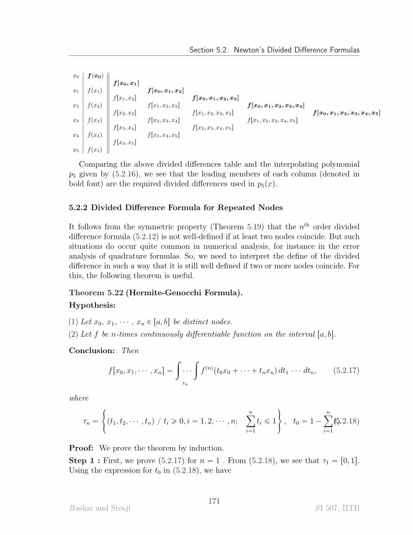
Section 5.2. Newton’s Divided Difference Formulas
x0 fpx0q
f rx0, x1s
x1 fpx1q f rx0, x1, x2s
f rx1, x2s f rx0, x1, x2, x3s
x2 fpx2q f rx1, x2, x3s f rx0, x1, x2, x3, x4s
f rx2, x3s f rx1, x2, x3, x4s f rx0, x1, x2, x3, x4, x5s
x3 fpx3q f rx2, x3, x4s f rx1, x2, x3, x4, x5s
f rx3, x4s f rx2, x3, x4, x5s
x4 fpx4q f rx3, x4, x5s
f rx4, x5s
x5 fpx5q
Comparing the above divided differences table and the interpolating polynomialp5 given by (5.2.16), we see that the leading members of each column (denoted inbold font) are the required divided differences used in p5pxq.
5.2.2 Divided Difference Formula for Repeated Nodes
It follows from the symmetric property (Theorem 5.19) that the nth order divideddifference formula (5.2.12) is not well-defined if at least two nodes coincide. But suchsituations do occur quite common in numerical analysis, for instance in the erroranalysis of quadrature formulas. So, we need to interpret the define of the divideddifference in such a way that it is still well defined if two or more nodes coincide. Forthis, the following theorem is useful.
Theorem 5.22 (Hermite-Genocchi Formula).
Hypothesis:
(1) Let x0, x1, ¨ ¨ ¨ , xn P ra, bs be distinct nodes.
(2) Let f be n-times continuously differentiable function on the interval ra, bs.
Conclusion: Then
f rx0, x1, ¨ ¨ ¨ , xns “
ż
¨ ¨ ¨
ż
τn
f pnqpt0x0 ` ¨ ¨ ¨ ` tnxnq dt1 ¨ ¨ ¨ dtn, (5.2.17)
where
τn “
#
pt1, t2, ¨ ¨ ¨ , tnq { ti ě 0, i “ 1, 2, ¨ ¨ ¨ , n;nÿ
i“1
ti ď 1
+
, t0 “ 1 ´
nÿ
i“1
ti.(5.2.18)
Proof: We prove the theorem by induction.
Step 1 : First, we prove (5.2.17) for n “ 1 . From (5.2.18), we see that τ1 “ r0, 1s.Using the expression for t0 in (5.2.18), we have
Baskar and Sivaji171
S I 507, IITB
Chapter 5. Interpolation
1ż
0
f 1pt0x0 ` t1x1qdt1 “
1ż
0
f 1px0 ` t1px1 ´ x0qq dt1 “1
x1 ´ x0fpx0 ` t1px1 ´ x0qq
ˇ
ˇ
ˇ
t1“1
t1“0
“fpx1q ´ fpx0q
x1 ´ x0“ f rx0, x1s.
Thus, we have proved the result (5.2.17) for n “ 1.
Step 2 : Now assume that the formula (5.2.17) holds for n “ k ě 1 and prove theformula for n “ k ` 1. We haveż
¨ ¨ ¨
ż
τk`1
f pk`1qpt0x0 ` t1x1 ` ¨ ¨ ¨ ` tk`1xk`1q dt1 ¨ ¨ ¨ dtk`1
“
ż
¨ ¨ ¨
ż
τk
¨
˝
1´pt1`¨¨¨`tkqż
0
f pk`1qpx0 ` t1px1 ´ x0q ` ¨ ¨ ¨ ` tk`1pxk`1 ´ x0qq dtk`1
˛
‚dt1 ¨ ¨ ¨ dtk
“
ż
¨ ¨ ¨
ż
τk
1
xk`1 ´ x0
“
f pkqpx0 ` t1px1 ´ x0q ` ¨ ¨ ¨ ` tk`1pxk`1 ´ x0qq‰tk`1“1´pt1`¨¨¨`tkq
tk`1“0dt1 ¨ ¨ ¨ dtk
“1
xk`1 ´ x0
»
–
ż
¨ ¨ ¨
ż
τk
f pkqpxk`1 ` t1px1 ´ xk`1q ` ¨ ¨ ¨ ` tkpxk ´ xk`1qq dt1 ¨ ¨ ¨ dtk
´
ż
¨ ¨ ¨
ż
τk
f pkqpx0 ` t1px1 ´ x0q ` ¨ ¨ ¨ ` tkpxk ´ x0qq dt1 ¨ ¨ ¨ dtk
fi
fl
“f rx1, ¨ ¨ ¨ , xk, xk`1s ´ f rx0, x1, ¨ ¨ ¨ , xks
xk`1 ´ x0“ f rx0, x1, ¨ ¨ ¨ , xk`1s.
By the principle of mathematical induction, the result is true for all n P N. [\
Remark 5.23. Since f is n-times continuously differentiable, the right hand side of(5.2.17) is meaningful for any set of points x0, x1, ¨ ¨ ¨ , xn, which are not necessarilydistinct. This gives a meaning, which can be used to define the nth order divideddifference when x0, x1, ¨ ¨ ¨ , xn are not distinct (i.e., one or more points are repeated).[\
Following results are direct consequences of the above theorem.
Corollary 5.24.
Hypothesis:
(1) Let x0, x1, ¨ ¨ ¨ , xn P ra, bs be a set of points, not necessarily distinct.
Baskar and Sivaji172
S I 507, IITB
Section 5.2. Newton’s Divided Difference Formulas
(2) Let f be n times continuously differentiable function on the interval ra, bs.
Conclusion:
(1) The function px0, x1, ¨ ¨ ¨ , xnq ÞÝÑ f rx0, x1, ¨ ¨ ¨ , xns is continuous on Rn`1.
(2) For any x P ra, bs, the limit
limpx0,x1,¨¨¨ ,xnqÑpx,x,¨¨¨ ,xq
f rx0, x1, ¨ ¨ ¨ , xns
exists and this limit is the nth-order divided difference f rx, x, ¨ ¨ ¨ , xs (x repeatedpn ` 1q-times). Further, we have
f rx, x, ¨ ¨ ¨ , xs “f pnqpxq
n!. (5.2.19)
Proof.
(1) The proof is out side the scope of this course and hence omitted.
(2) The proof follows from the fact that
ż
¨ ¨ ¨
ż
τn
1 dt1 ¨ ¨ ¨ dtn “1
n!
and the Hermite-Genocchi formula (5.2.17). [\
The following theorem gives an expression for the divided difference of an pn` 2q-times differentiable function when two nodes are repeated.
Theorem 5.25.
Hypothesis:
(1) Let x0, x1, ¨ ¨ ¨ , xn be given (distinct) nodes in an interval ra, bs.
(2) Let x P ra, bs, x R tx0, x1, ¨ ¨ ¨ , xnu.
Conclusion: The pn` 2qnd-order divided difference f rx0, x1, ¨ ¨ ¨ , xn, x, xs of an pn`
2q-times continuously differentiable function f is given by
f rx0, x1, ¨ ¨ ¨ , xn, x, xs “d
dxf rx0, x1, ¨ ¨ ¨ , xn, xs. (5.2.20)
Proof: It follows from (5.2.17) that the function F pxq “ f rx0, x1, ¨ ¨ ¨ , xn, xs for allx P ra, bs is well-defined and continuous. Therefore, using the symmetry property ofthe divided differences, we get
Baskar and Sivaji173
S I 507, IITB
Chapter 5. Interpolation
f rx0, x1, ¨ ¨ ¨ , xn, x, xs “ limhÑ0
f rx0, x1, ¨ ¨ ¨ , xn, x, x ` hs
“ limhÑ0
f rx, x0, x1, ¨ ¨ ¨ , xn, x ` hs.
As all the points used on the right hand side are distinct, we can use the formula(5.2.12) to get
f rx0, x1, ¨ ¨ ¨ , xn, x, xs “ limhÑ0
f rx0, x1, ¨ ¨ ¨ , xn, x ` hs ´ f rx, x0, x1, ¨ ¨ ¨ , xns
h
“ limhÑ0
f rx0, x1, ¨ ¨ ¨ , xn, x ` hs ´ f rx0, x1, ¨ ¨ ¨ , xn, xs
h
“d
dxf rx0, x1, ¨ ¨ ¨ , xn, xs.
This completes the proof. [\
5.3 Error in Polynomial Interpolation
Let f be a function defined on an interval I “ ra, bs. Let pnpxq be a polynomial ofdegree less than or equal to n that interpolates the function f at n` 1 nodes x0, x1,¨ ¨ ¨ , xn in I. How well does pnpxq approximate f on the interval I? This questionleads to the analysis of interpolation error.
As we discussed at the beginning of Chapter 2, the error given by
MEnpxq “ fpxq ´ pnpxq. (5.3.21)
is the mathematical error involved in the interpolating polynomial. But, whenwe perform the calculations using finite precision floating-point arithmetic, then thepolynomial obtained, denoted by pnpxq, need not be the same as the interpolatingpolynomial pnpxq. The error
AEnpxq “ pnpxq ´ pnpxq. (5.3.22)
is the arithmetic error involved in the interpolating polynomial.
The total error, denoted by TEnpxq, involved in the polynomial interpolation istherefore given by
TEnpxq “ fpxq ´ pnpxq “ pfpxq ´ pnpxqq ` ppnpxq ´ pnpxqq “ MEnpxq ` AEnpxq.
In Subsection 5.3.1, we derive the mathematical error involved in polynomial inter-polation. We analyze the effect of arithmetic error in Subsection 5.3.2.
Baskar and Sivaji174
S I 507, IITB
Section 5.3. Error in Polynomial Interpolation
5.3.1 Mathematical Error
The following theorem provides a formula for the interpolation error when we assumethat the necessary data are given exactly without any floating-point approximation.
Theorem 5.26 (Mathematical Error in Interpolation). Let pnpxq be the poly-nomial interpolating a function f P Cn`1ra, bs at the nodes x0, x1, ¨ ¨ ¨ , xn lying inI “ ra, bs. Then for each x P I, there exists a ξx P pa, bq such that
MEnpxq “f pn`1qpξxq
pn ` 1q!
nź
i“0
px ´ xiq (5.3.23)
Proof: If x is one of the nodes, then (5.3.23) holds trivially for any choice of ξx P pa, bq.Therefore, it is enough to prove the theorem when x is not a node. The idea is toobtain a function having at least n`2 distinct zeros; and then apply Rolle’s theoremn ` 1 times to get the desired conclusion.
For a given x P I with x ‰ xi pi “ 0, 1, ¨ ¨ ¨ , nq, define a new function ψ on theinterval I by
ψptq “ fptq ´ pnptq ´ λnź
i“0
pt ´ xiq, t P I, (5.3.24)
where λ is chosen so that ψpxq “ 0. This gives
λ “fpxq ´ pnpxq
nź
i“0
px ´ xiq
.
Note that ψpxiq “ 0 for each i “ 0, 1, ¨ ¨ ¨ , n. Thus, ψ has at least n ` 2 distinctzeros. By Rolle’s theorem, the function ψ1 has at least n ` 1 distinct zeros in pa, bq.A repeated application of Rolle’s theorem n ` 1 times to the function ψ gives thatψpn`1q has at least one zero in pa, bq; call it ξx. Differentiating (5.3.24) pn ` 1q-timesand noting that
ppn`1qn ptq “ 0,
˜
nź
i“0
pt ´ xiq
¸pn`1q
“ pn ` 1q!, ψpn`1qpξxq “ 0,
we see that ξx satisfies
0 “ ψpn`1qpξxq “ f pn`1qpξxq ´fpxq ´ pnpxq
nź
i“0
px ´ xiq
pn ` 1q !.
Thus,
Baskar and Sivaji175
S I 507, IITB
Chapter 5. Interpolation
f pn`1qpξxq ´MEnpxqnź
i“0
px ´ xiq
pn ` 1q ! “ 0.
The last equation yields (5.3.23). [\
The following theorem plays an important role in the error analysis of numericalintegration. The idea behind the proof of this theorem is similar to the idea used inthe above theorem and is left as an exercise.
Theorem 5.27. If f P Cn`1ra, bs and if x0, x1, ¨ ¨ ¨ , xn are distinct nodes in ra, bs,then for any x ‰ xi, i “ 0, 1, ¨ ¨ ¨ , n, there exists a point ξx P pa, bq such that
f rx0, x1, ¨ ¨ ¨ , xn, xs “f pn`1qpξxq
pn ` 1q !. (5.3.25)
Remark 5.28. It is interesting to note that when all the nodes coincide, then (5.3.25)reduces to (14). [\
Definition 5.29 (Infinity Norm).
If f is continuous on a closed interval I “ ra, bs, then the infinity norm of f ,denoted by }f}8,I , is defined as
}f}8,I “ maxxPI
|fpxq|. (5.3.26)
Example 5.30. Let us obtain an upper bound of the mathematical error for thelinear interpolating polynomial with respect to the infinity norm. As in Example5.10, the linear interpolating polynomial for f at x0 and x1 (x0 ă x1) is given by
p1pxq “ fpx0q ` f rx0, x1spx ´ x0q,
where f rx0, x1s is given by (5.2.10). For each x P I :“ rx0, x1s, using the formula(5.3.23), the error ME1pxq is given by
ME1pxq “px ´ x0qpx ´ x1q
2f 2pξxq,
where ξx P px0, x1q depends on x. Therefore,
|ME1pxq| ď |px ´ x0qpx ´ x1q|}f2}8,I
2.
Note that the maximum value of |px´x0qpx´x1q| as x varies in the interval rx0, x1s,occurs at x “ px0 ` x1q{2. Therefore, we have
|px ´ x0qpx ´ x1q| ďpx1 ´ x0q
2
4.
Baskar and Sivaji176
S I 507, IITB
Section 5.3. Error in Polynomial Interpolation
Using this inequality, we get an upper bound
|ME1pxq| ď px1 ´ x0q2 }f2}8,I
8, for all x P rx0, x1s.
Note that the above inequality is true for all x P rx0, x1s. In particular, this inequalityis true for an x at with the function |ME1| attains its maximum. Thus, we have
}ME1}8,I ď px1 ´ x0q2 }f 2}8,I
8.
The right hand side quantity, which is a real number, is an upper bound for themathematical error in linear interpolation with respect to the infinity norm. [\
Example 5.31. Let the function
fpxq “ sinx
be approximated by an interpolating polynomial p9pxq of degree less than or equalto 9 for f at the nodes x0, x1, ¨ ¨ ¨ , x9 in the interval I :“ r0, 1s. Let us obtain anupper bound for }ME9}8,I , where (from (5.3.23))
ME9pxq “f p10qpξxq
10!
9ź
i“0
px ´ xiq.
Since |f p10qpξxq| ď 1 andś9
i“0 |x ´ xi| ď 1, we have
| sinx ´ p9pxq| “ |ME9pxq| ď1
10!ă 2.8 ˆ 10´7, for all x P r0, 1s.
Since this holds for all x P r0, 1s, we have
}ME9}8,I ă 2.8 ˆ 10´7.
The right hand side number is the upper bound for the mathematical error ME9 withrespect to the infinity norm on the interval I [\
5.3.2 Arithmetic Error
Quite often, the polynomial interpolation that we compute is based on the functiondata subjected to floating-point approximation. In this subsection, we analyze thearithmetic error arising due to the floating-point approximation flpfpxiqq of fpxiq foreach node point xi, i “ 0, 1, ¨ ¨ ¨ , n in the interval I “ ra, bs.
The Lagrange form of interpolating polynomial that uses the values flpfpxiqq in-stead of fpxiq, i “ 0, 1, ¨ ¨ ¨ , n is given by
Baskar and Sivaji177
S I 507, IITB
Chapter 5. Interpolation
pnpxq “
nÿ
i“0
flpfpxiqq lipxq.
We now analyze the arithmetic error. Denoting
ϵi :“ fpxiq ´ flpfpxiq; ||ϵ||8 “ maxt|ϵi| : i “ 0, 1, ¨ ¨ ¨ , nu,
we have
|AEnpxq| “ |pnpxq ´ pnpxq| “
ˇ
ˇ
ˇ
ˇ
ˇ
nÿ
i“0
´
fpxiq ´ flpfpxiqq
¯
lipxq
ˇ
ˇ
ˇ
ˇ
ˇ
ď ||ϵ||8
nÿ
i“0
||li||8,I ,
for all x P I. Therefore,
}AEn}8,I “ }pn ´ pn}8,I ď ||ϵ||8
nÿ
i“0
||li||8,I . (5.3.27)
The upper bound in (5.3.27) might grow quite large as n increases, especially whenthe nodes are equally spaced as we will study now.
Assume that the nodes are equally spaced in the interval ra, bs, with x0 “ a andxn “ b, and xi`1 ´ xi “ h for all i “ 0, 1, ¨ ¨ ¨ , n ´ 1. Note that h “ pb ´ aq{n. Wewrite
xi “ a ` ih, i “ 0, 1, ¨ ¨ ¨ , n.
Any x P I can be written asx “ a ` ηh,
where 0 ď η ď n. Here η is not necessarily an integer. Therefore, for any x P I, wehave
lkpxq “
nź
i“0i‰k
px ´ xiq
pxk ´ xiq“
nź
i“0i‰k
pη ´ iq
pk ´ iq, k “ 0, ¨ ¨ ¨ , n.
Clearly, the Lagrange polynomials are not dependent on the choice of a, b, and h.They depend entirely on n and η (which depends on x). The Figure 5.2 (a), (b) and(c) shows the function
lpxq “
nÿ
i“0
|lipxq| (5.3.28)
for n “ 2, 8 and 18. It is observed that as n increases, the maximum of the functionl increases. In fact, as n Ñ 8, the maximum of l tends to infinity and it is observedin Figure 5.2 (d) which depicts n in the x-axis and the function
Mn “
nÿ
i“0
||li||8,I (5.3.29)
Baskar and Sivaji178
S I 507, IITB
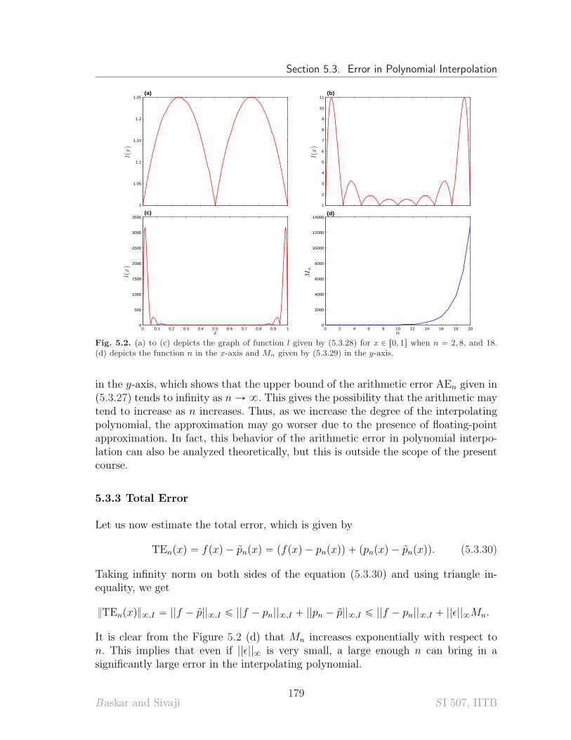
Section 5.3. Error in Polynomial Interpolation
0 0.1 0.2 0.3 0.4 0.5 0.6 0.7 0.8 0.9 11
1.05
1.1
1.15
1.2
1.25
x
l(x)
(a)
0 0.1 0.2 0.3 0.4 0.5 0.6 0.7 0.8 0.9 11
2
3
4
5
6
7
8
9
10
11
x
l(x)
(b)
0 0.1 0.2 0.3 0.4 0.5 0.6 0.7 0.8 0.9 10
500
1000
1500
2000
2500
3000
3500
x
l(x)
(c)
0 2 4 6 8 10 12 14 16 18 200
2000
4000
6000
8000
10000
12000
14000
n
Mn
(d)
Fig. 5.2. (a) to (c) depicts the graph of function l given by (5.3.28) for x P r0, 1s when n “ 2, 8, and 18.(d) depicts the function n in the x-axis and Mn given by (5.3.29) in the y-axis.
in the y-axis, which shows that the upper bound of the arithmetic error AEn given in(5.3.27) tends to infinity as n Ñ 8. This gives the possibility that the arithmetic maytend to increase as n increases. Thus, as we increase the degree of the interpolatingpolynomial, the approximation may go worser due to the presence of floating-pointapproximation. In fact, this behavior of the arithmetic error in polynomial interpo-lation can also be analyzed theoretically, but this is outside the scope of the presentcourse.
5.3.3 Total Error
Let us now estimate the total error, which is given by
TEnpxq “ fpxq ´ pnpxq “ pfpxq ´ pnpxqq ` ppnpxq ´ pnpxqq. (5.3.30)
Taking infinity norm on both sides of the equation (5.3.30) and using triangle in-equality, we get
}TEnpxq}8,I “ ||f ´ p||8,I ď ||f ´ pn||8,I ` ||pn ´ p||8,I ď ||f ´ pn||8,I ` ||ϵ||8Mn.
It is clear from the Figure 5.2 (d) that Mn increases exponentially with respect ton. This implies that even if ||ϵ||8 is very small, a large enough n can bring in asignificantly large error in the interpolating polynomial.
Baskar and Sivaji179
S I 507, IITB
Chapter 5. Interpolation
Thus, for a given function and a set of equally spaced nodes, even if the mathe-matical error is bounded, the presence of floating-point approximation in the givendata can lead to significantly large arithmetic error for larger values of n.
5.3.4 Runge Phenomenon
In the previous section, we have seen that even a small arithmetic error may leadto a drastic magnification of total error as we go on increasing the degree of thepolynomial. This gives us a feeling that if the calculation is done with infinite precision(that is, without any finite digit floating point arithmetic) and the function f issmooth, then we always have a better approximation for a larger value of n. In otherwords, we expect
limnÑ8
}f ´ pn}8,I “ 0.
But this is not true in the case of equally spaced nodes. This was first shown by CarlRunge, where he discovered that there are certain functions for which, as we go onincreasing the degree of interpolating polynomial, the total error increases drasticallyand the corresponding interpolating polynomial oscillates near the boundary of theinterval in which the interpolation is done. Such a phenomenon is called the RungePhenomenon. This phenomenon is well understood by the following example givenby Runge.
Example 5.32 (Runge’s Function). Consider the Runge’s function defined onthe interval r´1, 1s given by
fpxq “1
1 ` 25x2. (5.3.31)
The interpolating polynomials with n “ 2, n “ 8 and n “ 18 are depicted in Figure5.3. This figure clearly shows that as we increase the degree of the polynomial, theinterpolating polynomial differs significantly from the actual function especially, nearthe end points of the interval. [\
In the light of the discussion made in Subsection 5.3.2, we may think that theRunge phenomenon is due to the amplification of the arithmetic error. But, even ifthe calculation is done with infinite precision (that is, without any finite digit floatingpoint arithmetic), we may still have the Runge phenomenon due to the amplificationin mathematical error. This can be observed by taking infinity norm on both sides ofthe formula (5.3.23). This gives the upper bound of the infinity norm of MEnpxq as
}MEn}8,I ďpb ´ aqn`1
pn ` 1q!}f pn`1q}8,I .
Although the first part, pb´aqn`1{pn`1q! in the upper bound tends to zero as n Ñ 8,if the second part, }f pn`1q}8,I increases significantly as n increases, then the upper
Baskar and Sivaji180
S I 507, IITB
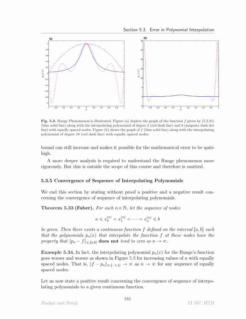
Section 5.3. Error in Polynomial Interpolation
−1 −0.8 −0.6 −0.4 −0.2 0 0.2 0.4 0.6 0.8 1
−1
−0.8
−0.6
−0.4
−0.2
0
0.2
0.4
0.6
0.8
1
x
pn(x)
(a)
−1 −0.8 −0.6 −0.4 −0.2 0 0.2 0.4 0.6 0.8 1−5
0
5
10
15
20
25
30
x
pn(x)
(b)
Fig. 5.3. Runge Phenomenon is illustrated. Figure (a) depicts the graph of the function f given by (5.3.31)(blue solid line) along with the interpolating polynomial of degree 2 (red dash line) and 8 (magenta dash dotline) with equally spaced nodes. Figure (b) shows the graph of f (blue solid line) along with the interpolatingpolynomial of degree 18 (red dash line) with equally spaced nodes.
bound can still increase and makes it possible for the mathematical error to be quitehigh.
A more deeper analysis is required to understand the Runge phenomenon morerigorously. But this is outside the scope of this course and therefore is omitted.
5.3.5 Convergence of Sequence of Interpolating Polynomials
We end this section by stating without proof a positive and a negative result con-cerning the convergence of sequence of interpolating polynomials.
Theorem 5.33 (Faber). For each n P N, let the sequence of nodes
a ď xpnq
0 ă xpnq
1 ă ¨ ¨ ¨ ă xpnqn ď b
be given. Then there exists a continuous function f defined on the interval ra, bs suchthat the polynomials pnpxq that interpolate the function f at these nodes have theproperty that }pn ´ f}8,ra,bs does not tend to zero as n Ñ 8.
Example 5.34. In fact, the interpolating polynomial pnpxq for the Runge’s functiongoes worser and worser as shown in Figure 5.3 for increasing values of n with equallyspaced nodes. That is, }f ´ pn}8,r´1,1s Ñ 8 as n Ñ 8 for any sequence of equallyspaced nodes.
Let us now state a positive result concerning the convergence of sequence of interpo-lating polynomials to a given continuous function.
Baskar and Sivaji181
S I 507, IITB
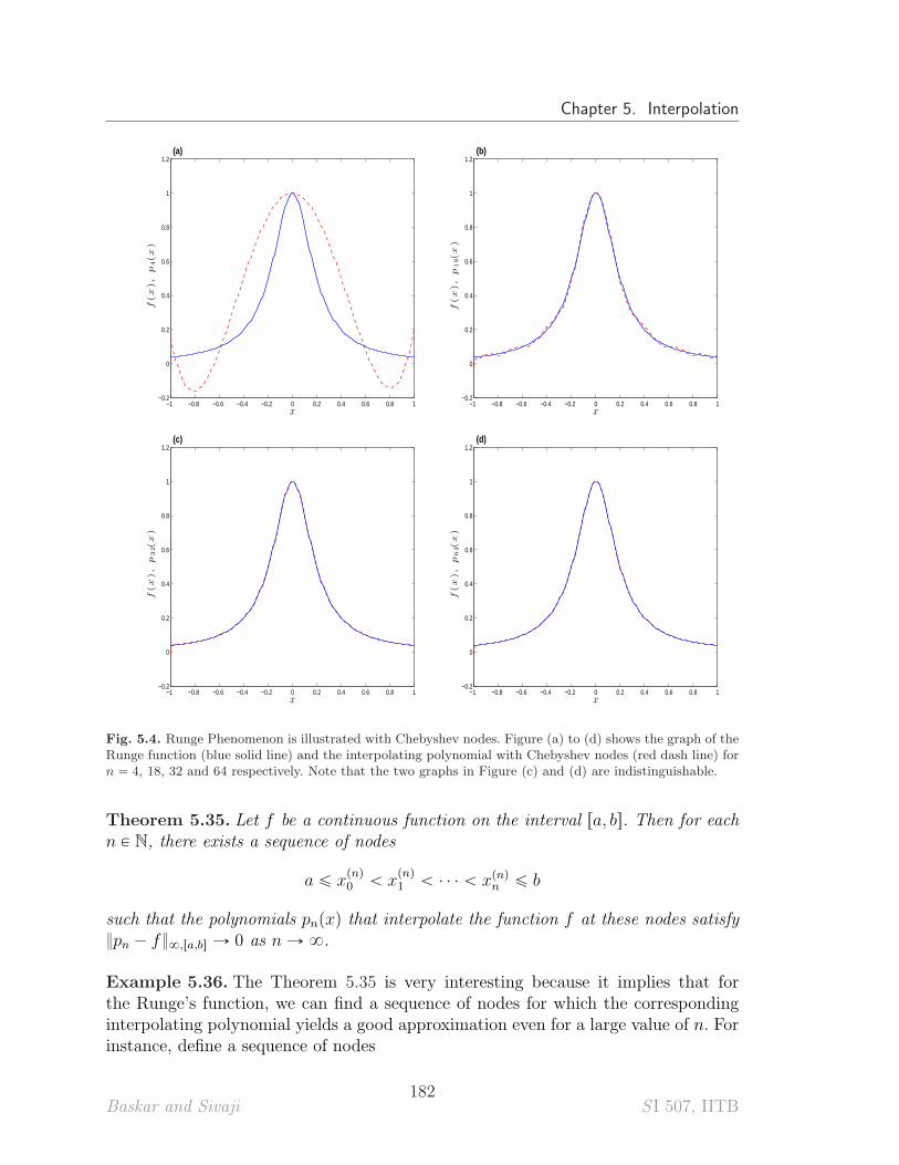
Chapter 5. Interpolation
−1 −0.8 −0.6 −0.4 −0.2 0 0.2 0.4 0.6 0.8 1−0.2
0
0.2
0.4
0.6
0.8
1
1.2
x
f(x),p4(x)
(a)
−1 −0.8 −0.6 −0.4 −0.2 0 0.2 0.4 0.6 0.8 1−0.2
0
0.2
0.4
0.6
0.8
1
1.2
x
f(x),p18(x)
(b)
−1 −0.8 −0.6 −0.4 −0.2 0 0.2 0.4 0.6 0.8 1−0.2
0
0.2
0.4
0.6
0.8
1
1.2
x
f(x),p32(x)
(c)
−1 −0.8 −0.6 −0.4 −0.2 0 0.2 0.4 0.6 0.8 1−0.2
0
0.2
0.4
0.6
0.8
1
1.2
x
f(x),p64(x)
(d)
Fig. 5.4. Runge Phenomenon is illustrated with Chebyshev nodes. Figure (a) to (d) shows the graph of theRunge function (blue solid line) and the interpolating polynomial with Chebyshev nodes (red dash line) forn “ 4, 18, 32 and 64 respectively. Note that the two graphs in Figure (c) and (d) are indistinguishable.
Theorem 5.35. Let f be a continuous function on the interval ra, bs. Then for eachn P N, there exists a sequence of nodes
a ď xpnq
0 ă xpnq
1 ă ¨ ¨ ¨ ă xpnqn ď b
such that the polynomials pnpxq that interpolate the function f at these nodes satisfy}pn ´ f}8,ra,bs Ñ 0 as n Ñ 8.
Example 5.36. The Theorem 5.35 is very interesting because it implies that forthe Runge’s function, we can find a sequence of nodes for which the correspondinginterpolating polynomial yields a good approximation even for a large value of n. Forinstance, define a sequence of nodes
Baskar and Sivaji182
S I 507, IITB
Section 5.4. Piecewise Polynomial Interpolation
xpnq
i “ cos
ˆ
p2i ` 1qπ
2pn ` 1q
˙
, i “ 0, 1, ¨ ¨ ¨ , n (5.3.32)
for each n “ 0, 1, 2, ¨ ¨ ¨ . When n “ 4, the nodes are xp4q
0 “ cospπ{10q, xp4q
1 “
cosp3π{10q, xp4q
2 “ cosp5π{10q, xp4q
3 “ cosp7π{10q and x44 “ cosp9π{10q. The nodes
xpnq
i defined by (5.3.32) are called Chebyshev nodes.
Figure 5.4 depicts pnpxq for n “ 4, 18, 32, and 64 along with the Runge’s function.From these figures, we observe that the interpolating polynomial pnpxq agrees wellwith the Runge’s function. [\
5.4 Piecewise Polynomial Interpolation
Quite often polynomial interpolation will be unsatisfactory as an approximation tool.This is true if we insist on letting the order of the polynomial get larger and larger.However, if we keep the order of the polynomial fixed, and use different polynomialsover different intervals, with the length of the intervals getting smaller and smaller,then the resulting interpolating function approximates the given function more ac-curately.
Let us start with linear interpolation over an interval I “ ra, bs which leads to
p1pxq “ fpaq ` f ra, bspx ´ aq “ fpaq `fpbq ´ fpaq
b ´ apx ´ aq “
x ´ b
a ´ bfpaq `
x ´ a
b ´ afpbq,
where the nodes are x0 “ a, x2 “ b. In addition to these two nodes, we now chooseone more point x1 such that x0 ă x1 ă x2. With these three nodes, can obtain aquadratic interpolation polynomial. Instead, we can interpolate the function fpxq inrx0, x1s by a linear polynomial with nodes x0 and x1, and in rx1, x2s by another linearpolynomial with nodes x1 and x2. Such polynomials are given by
p1,1pxq :“x ´ x1x0 ´ x1
fpx0q `x ´ x0x1 ´ x0
fpx1q, p1,2pxq :“x ´ x2x1 ´ x2
fpx1q `x ´ x1x2 ´ x1
fpx2q
and the interpolating function is given by
spxq “
"
p1,1pxq , x P rx0, x1sp1,2pxq , x P rx1, x2s
.
Note that spxq is a continuous function on rx0, x2s, which interpolates fpxq and islinear in rx0, x1s and rx1, x2s. Such an interpolating function is called piecewiselinear interpolating function.
In a similar way as done above, we can also obtain piecewise quadratic, cubicinterpolating functions and so on.
Baskar and Sivaji183
S I 507, IITB
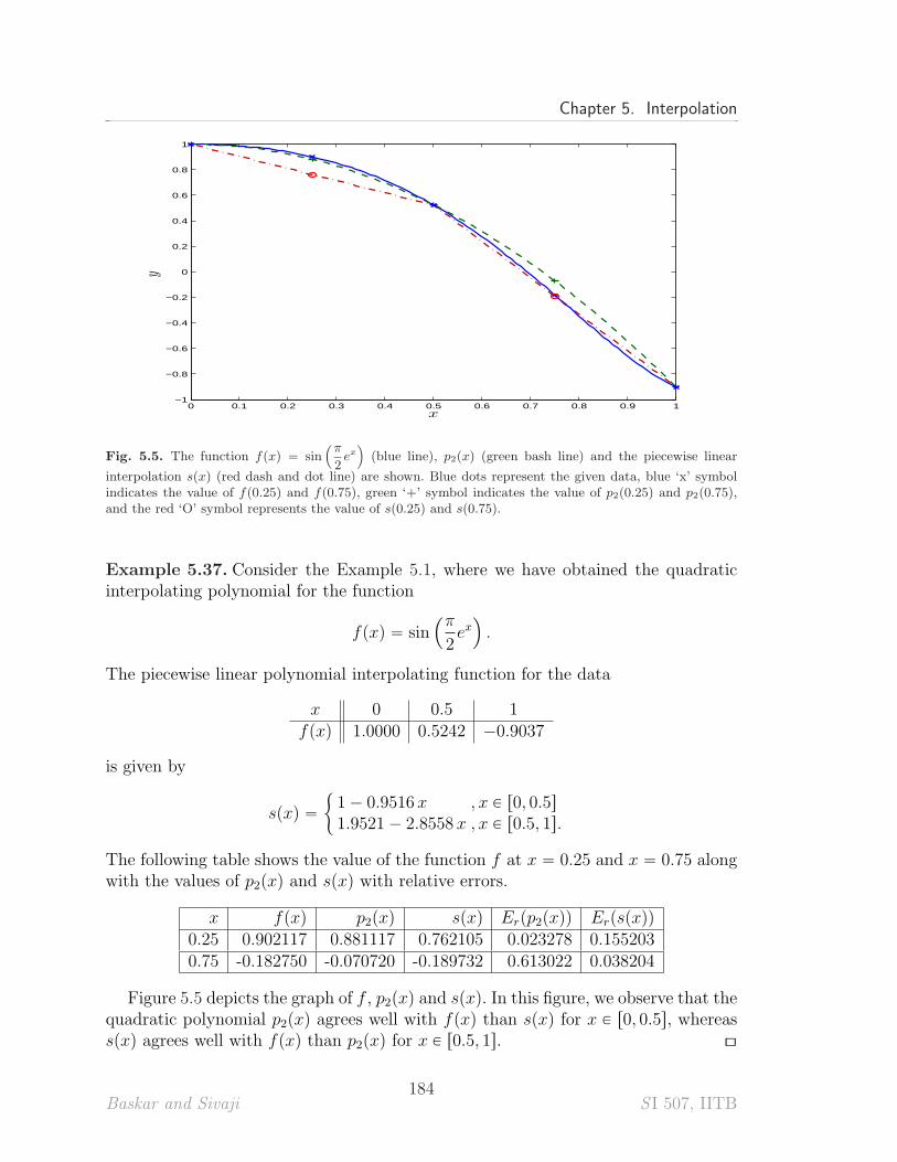
Chapter 5. Interpolation
0 0.1 0.2 0.3 0.4 0.5 0.6 0.7 0.8 0.9 1−1
−0.8
−0.6
−0.4
−0.2
0
0.2
0.4
0.6
0.8
1
x
y
Fig. 5.5. The function fpxq “ sin´π
2ex¯
(blue line), p2pxq (green bash line) and the piecewise linear
interpolation spxq (red dash and dot line) are shown. Blue dots represent the given data, blue ‘x’ symbolindicates the value of fp0.25q and fp0.75q, green ‘+’ symbol indicates the value of p2p0.25q and p2p0.75q,and the red ‘O’ symbol represents the value of sp0.25q and sp0.75q.
Example 5.37. Consider the Example 5.1, where we have obtained the quadraticinterpolating polynomial for the function
fpxq “ sin´π
2ex¯
.
The piecewise linear polynomial interpolating function for the data
x 0 0.5 1fpxq 1.0000 0.5242 ´0.9037
is given by
spxq “
"
1 ´ 0.9516 x , x P r0, 0.5s
1.9521 ´ 2.8558x , x P r0.5, 1s.
The following table shows the value of the function f at x “ 0.25 and x “ 0.75 alongwith the values of p2pxq and spxq with relative errors.
x fpxq p2pxq spxq Erpp2pxqq Erpspxqq
0.25 0.902117 0.881117 0.762105 0.023278 0.1552030.75 -0.182750 -0.070720 -0.189732 0.613022 0.038204
Figure 5.5 depicts the graph of f , p2pxq and spxq. In this figure, we observe that thequadratic polynomial p2pxq agrees well with fpxq than spxq for x P r0, 0.5s, whereasspxq agrees well with fpxq than p2pxq for x P r0.5, 1s. [\
Baskar and Sivaji184
S I 507, IITB
Section 5.5. Spline Interpolation
5.5 Spline Interpolation
Although a piecewise interpolating function introduced in Section 5.4 is continuous,it may not be differentiable at the nodes. We wish to find an interpolating functionthat is sufficiently smooth and does a better approximation to fpxq. This can beachieved by spline interpolation.
Definition 5.38 (Spline Interpolating Function).
A spline interpolating function of degree d with nodes xi, i “ 0, 1, ¨ ¨ ¨ , n (x0 ă
x1 ă ¨ ¨ ¨ ă xn) is a function spxq with the following properties
(1) On each subinterval rxi´1, xis, i “ 1, 2, ¨ ¨ ¨ , n, spxq is a polynomial of degree lessthan or equal to d.
(2) spxq and its first (d ´ 1) derivatives are continous on rx0, xns.
(3) The interpolation conditions spxiq “ fpxiq, i “ 0, 1, ¨ ¨ ¨ , n are satisfied.
We shall now study how we can obtain the interpolation of a function f as splineinterpolating functions instead of polynomials. For the sake of simplicity, we restrictonly to d “ 3, called the cubic spline interpolating function.
Remark 5.39. Note that in each subinterval rxi´1, xis, i “ 1, 2, ¨ ¨ ¨ , n, we only knowfpxi´1q and fpxiq. But we look for a cubic polynomial in this subinterval. Therefore,we cannot follow the Lagrange’s or Newton’s interpolating formula, as these formulasdemand the function values at four distinct nodes in the subinterval. We need toadopt a different method for the construction of the polynomial in each subintervalin order to obtain the spline interpolation. [\
Construction of a Cubic Spline
The construction of a cubic spline interpolating function spxq of a function fpxq isas follows:
Step 1: Let us denote by M1, ¨ ¨ ¨ , Mn,
Mi “ s2pxiq, i “ 0, 1, ¨ ¨ ¨ , n
and first obtain spxq in terms of Mi’s which are unknowns.
Step 2: Since spxq is cubic on each rxi´1, xis, the function s2pxq is linear on theinterval such that
s2pxi´1q “ Mi´1, s2pxiq “ Mi.
Therefore, it is given by
s2pxq “pxi ´ xqMi´1 ` px ´ xi´1qMi
xi ´ xi´1
, xi´1 ď x ď xi (5.5.33)
Baskar and Sivaji185
S I 507, IITB
Chapter 5. Interpolation
Integrating (5.5.33) two times with respect to x, we get
spxq “pxi ´ xq3Mi´1
6pxi ´ xi´1q`
px ´ xi´1q3Mi
6pxi ´ xi´1q` K1x ` K2,
where K1 and K2 are integrating constants to be determined by using the interpola-tion conditions spxi´1q “ fpxi´1q and spxiq “ fpxiq. We have
K1 “fpxiq ´ fpxi´1q
xi ´ xi´1
´pMi ´ Mi´1qpxi ´ xi´1q
6
K2 “xifpxi´1q ´ xi´1fpxiq
xi ´ xi´1
´pMi´1xi ´ Mixi´1qpxi ´ xi´1q
6
Substituting these values in the above equation, we get
spxq “pxi ´ xq3Mi´1 ` px ´ xi´1q
3Mi
6pxi ´ xi´1q`
pxi ´ xqfpxi´1q ` px ´ xi´1qfpxiq
xi ´ xi´1
´1
6pxi ´ xi´1qrpxi ´ xqMi´1 ` px ´ xi´1qMis, xi´1 ď x ď xi (5.5.34)
Formula (5.5.34) applies to each of the intervals rx1, x2s, ¨ ¨ ¨ , rxn´1, xns. The formulasfor adjacent intervals rxi´1, xis and rxi, xi`1s will agree at their common point x “
xi because of the interpolating condition spxiq “ fpxiq. This implies that spxq iscontinuous over the entire interval ra, bs. Similarly, formula (5.5.33) for s2pxq impliesthat it is continuous on ra, bs.
Step 3: All that remains is to find the values of Mi for all i “ 0, 1, ¨ ¨ ¨ , n. This isobtained by ensuring the continuity of s1pxq over ra, bs, ie., the formula for s1pxq onrxi´1, xis and rxi, xi`1s are required to give the same value at their common pointx “ xi, for i “ 1, 2, ¨ ¨ ¨ , n ´ 1. After simplification, we get the system of linearequations for i “ 1, 2, ¨ ¨ ¨n ´ 1
xi ´ xi´1
6Mi´1 `
xi`1 ´ xi´1
3Mi `
xi`1 ´ xi6
Mi`1
“fpxi`1q ´ fpxiq
xi`1 ´ xi´fpxiq ´ fpxi´1q
xi ´ xi´1
.(5.5.35)
These n ´ 1 equations together with the assumption that
M0 “ Mn “ 0 (5.5.36)
leads to the values of M0, M1, ¨ ¨ ¨ , Mn and hence to the interpolation function spxq.
A spline constructed above is called a natural spline.
Example 5.40. Calculate the natural cubic spline interpolating the data"
p1, 1q,
ˆ
2,1
2
˙
,
ˆ
3,1
3
˙
,
ˆ
4,1
4
˙*
.
Baskar and Sivaji186
S I 507, IITB
Section 5.5. Spline Interpolation
The number of points is n “ 3 and xi ´ xi´1 “ 1, for x “ 1, 2, 3.Step 1: Here, we have
M0 “ s2p1q, M1 “ s2p2q, M2 “ s2p3q, M3 “ s2p4q.
Step 2: The function s2pxq is given by
s2pxq “
$
&
%
p2 ´ xqM0 ` px ´ 1qM1 , x P r1, 2s
p3 ´ xqM1 ` px ´ 2qM2 , x P r2, 3s
p4 ´ xqM2 ` px ´ 3qM3 , x P r3, 4s
.
Integrating s2pxq two times with respect to x, we get
spxq “
$
’
’
’
’
’
’
’
’
’
&
’
’
’
’
’
’
’
’
’
%
p2 ´ xq3M0
6`
px ´ 1q3M1
6` K1x ` K2 , x P r1, 2s
p3 ´ xq3M1
6`
px ´ 2q3M2
6` K1x ` K2 , x P r2, 3s
p4 ´ xq3M2
6`
px ´ 3q3M3
6` K1x ` K2 , x P r3, 4s
.
where K1 and K2 are integrating constants to be determined by using the conditionsspxi´1q “ fpxi´1q and spxiq “ fpxiq. We have
K1 “
$
’
’
’
’
’
’
’
’
&
’
’
’
’
’
’
’
’
%
´1
2´
pM1 ´ M0q
6, x P r1, 2s
´1
6´
pM2 ´ M1q
6, x P r2, 3s
´1
12´
pM3 ´ M2q
6, x P r3, 4s
.
K2 “
$
’
’
’
’
’
’
’
’
&
’
’
’
’
’
’
’
’
%
3
2´
2M0 ´ M1
6, x P r1, 2s
5
6´
3M1 ´ 2M2
6, x P r2, 3s
7
12´
4M2 ´ 3M3
6, x P r3, 4s
.
Substituting these expressions in the expression of spxq, we get the required cubicspline as given in (5.5.34).Step 3: Since we are constructing the natural spline, we take M0 “ M3 “ 0. The
Baskar and Sivaji187
S I 507, IITB
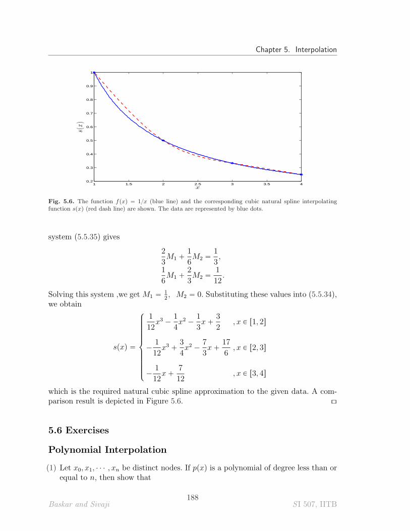
Chapter 5. Interpolation
1 1.5 2 2.5 3 3.5 40.2
0.3
0.4
0.5
0.6
0.7
0.8
0.9
1
x
s(x
)
Fig. 5.6. The function fpxq “ 1{x (blue line) and the corresponding cubic natural spline interpolatingfunction spxq (red dash line) are shown. The data are represented by blue dots.
system (5.5.35) gives
2
3M1 `
1
6M2 “
1
3,
1
6M1 `
2
3M2 “
1
12.
Solving this system ,we getM1 “ 12, M2 “ 0. Substituting these values into (5.5.34),
we obtain
spxq “
$
’
’
’
’
’
’
’
’
&
’
’
’
’
’
’
’
’
%
1
12x3 ´
1
4x2 ´
1
3x `
3
2, x P r1, 2s
´1
12x3 `
3
4x2 ´
7
3x `
17
6, x P r2, 3s
´1
12x `
7
12, x P r3, 4s
which is the required natural cubic spline approximation to the given data. A com-parison result is depicted in Figure 5.6. [\
5.6 Exercises
Polynomial Interpolation
(1) Let x0, x1, ¨ ¨ ¨ , xn be distinct nodes. If ppxq is a polynomial of degree less than orequal to n, then show that
Baskar and Sivaji188
S I 507, IITB
Section 5.6. Exercises
ppxq “
nÿ
i“0
ppxiqlipxq,
where lipxq is the ith Lagrange polynomial.
(2) Show that the polynomial 1` x` 2x2 is an interpolating polynomial for the data
x 0 1 2y 1 4 11
.
Find an interpolating polynomial for the new data
x 0 1 2 3y 1 4 11 -2
.
Does there exist a quadratic polynomial that satisfies the new data? Justify youranswer.
(3) The quadratic polynomial p2pxq “ 34x2 ` 1
4x ` 1
2interpolates the data
x ´1 0 1y 1 1
232
.
Find a node x3 (x3 R t´1, 0, 1u), and a real number y3 such that the polynomialp3pxq interpolating the data
x ´1 0 1 x3y 1 1{2 3{2 y3
is a polynomial of degree less than or equal to 2. (Quiz 1, Spring 2012)
(4) Let ppxq, qpxq, and rpxq be interpolating polynomials for the three sets of data
x 0 1y y0 y1
,x 0 2y y0 y2
, andx 1 2 3y y1 y2 y3
respectively. Let spxq be the the interpolating polynomial for the data
x 0 1 2 3y y0 y1 y2 y3
.
Ifppxq “ 1 ` 2x, qpxq “ 1 ` x, and rp2.5q “ 3,
then find the value of sp2.5q. (Quiz 1, Spring 2012)
(5) Obtain Lagrange form of interpolating polynomial for equally spaced nodes.
Baskar and Sivaji189
S I 507, IITB
Chapter 5. Interpolation
(6) Using Lagrange form of interpolating polynomial for the function gpxq “ 3x2 `
x ` 1, express the rational function
fpxq “3x2 ` x ` 1
px ´ 1qpx ´ 2qpx ´ 3q
as a sum of partial fractions.
(7) Find the Largrange form of interpolating polynomial for the data:
x -2 -1 1 3y -1 3 -1 19
(8) Find the Lagrange form of interpolating polynomial p2pxq that interpolates thefunction fpxq “ e´x2
at the nodes x0 “ ´1, x1 “ 0 and x2 “ 1. Further, find thevalue of p2p´0.9q (use 6-digit rounding). Compare the value with the true valuefp´0.9q (use 6-digit rounding). Find the percentage error in this calculation.
(9) Find the Newton form of interpolating polynomial for the data
x -3 -1 0 3 5y -30 -22 -12 330 3458
.
Newton’s Divided Difference Formula
(10) For the particular function fpxq “ xm (m P N), show that
f rx0, x1, ¨ ¨ ¨ , xns “
#
1 if n “ m
0 if n ą m
(11) Let x0, x1, ¨ ¨ ¨ , xn be nodes, and f be a given function. Define wpxq “śn
i“0px´xiq.Prove that
f rx0, x1, ¨ ¨ ¨ , xns “
nÿ
i“0
fpxiq
w1pxiq.
(12) Calculate the nth divided difference f rx0, x1, ¨ ¨ ¨ , xns of fpxq “1
x.
(13) The following data correspond to a polynomial P pxq of unknown degree
x 0 1 2P pxq 2 ´1 4
.
Determine the coefficient of x in the polynomial P pxq if all the third order divideddifferences are 1.
Baskar and Sivaji190
S I 507, IITB
Section 5.6. Exercises
(14) Let f be n times continuously differentiable function on the interval ra, bs. Forany x P ra, bs, show that the nth order divided difference f r x, x, ¨ ¨ ¨ , x
looooomooooon
pn`1q´times
s is given
by
f rx, x, ¨ ¨ ¨ , xlooooomooooon
pn`1q´times
s “f pnqpxq
n!.
(15) For the function fpxq “ sinpπxq, find the value of f r1{2, 0, 1, 1{2s.
Error in Polynomial Interpolation
(16) Prove that if we take any set of 23 nodes in the interval r´1, 1s and interpolatethe function fpxq “ coshx with a polynomial p22 of degree less than or equal to22, then at each x P r´1, 1s the relative error satisfies the bound
|fpxq ´ p22pxq|
|fpxq|ď 5 ˆ 10´16.
(17) Let pnpxq be a polynomial of degree less than or equal to n that interpolates afunction f at a set of distinct nodes x0, x1, ¨ ¨ ¨ , xn. If x R t x0, x1, ¨ ¨ ¨ , xn u, thenshow that the error is given by
fpxq ´ pnpxq “ f rx0, x1, ¨ ¨ ¨ , xn, xs
nź
i“0
px ´ xiq.
(18) If f P Cn`1ra, bs and if x0, x1, ¨ ¨ ¨ , xn are distinct nodes in ra, bs, then show thatthere exists a point ξx P pa, bq such that
f rx0, x1, ¨ ¨ ¨ , xn, xs “f pn`1qpξxq
pn ` 1q !
(19) Let N be a natural number. Let p1pxq denote the linear interpolating polynomialon the interval rN,N`1s interpolating the function fpxq “ x2 at the nodes N andN ` 1. Find an upper bound for the mathematical error ME1 using the infinitynorm on the interval rN,N ` 1s (i.e., }ME1}8, rN,N`1s).
(20) Let p3pxq denote a polynomial of degree less than or equal to 3 that interpolatesthe function fpxq “ lnx at the nodes x0 “ 1, x1 “ 4
3, x2 “ 5
3, x3 “ 2. Find a lower
bound on the absolute value of mathematical error |ME3pxq| at the point x “ 32,
using the formula for mathematical error in interpolation.
Baskar and Sivaji191
S I 507, IITB
Chapter 5. Interpolation
(21) Let f : r0, π6s Ñ R be a given function. The following is the meaning for the Cubic
interpolation in a table of function values (Final Exam, Spring 2012)
x x0 x1 ¨ ¨ ¨ xNfpxq fpx0q fpx1q ¨ ¨ ¨ fpxNq
The values of fpxq are tabulated for a set of equally spaced points in ra, bs, sayxi for i “ 0, 1, ¨ ¨ ¨ , N with x0 “ 0, xN “ π
6, and h “ xi`1 ´ xi ą 0 for every
i “ 0, 1, ¨ ¨ ¨ , N ´ 1. For an x P r0, π6s at which the function value fpxq is not
tabulated, the value of fpxq is taken to be the value of p3pxq, where p3pxq is thepolynomial of degree less than or equal to 3 that interpolates f at the nodesxi, xi`1, xi`2, xi`3 where i is the least index such that x P rxi, xi`3s.
Take fpxq “ sin x for x P r0, π6s; and answer the following questions.
(i) When x and p3 are as described above, then show that |fpxq ´ p3pxq| ď h4
48.
(ii) If h “ 0.005, then show that cubic interpolation in the table of function valuesyields the value of fpxq with at least 10 decimal-place accuracy.
(22) Let x0, x1, ¨ ¨ ¨ , xn be n ` 1 distinct nodes, and f be a function. For eachi “ 0, 1, ¨ ¨ ¨ , n, let fl pfpxiqq denote the floating point approximation of fpxiqobtained by rounding to 5 decimal places (note this is different from using 5-digit rounding). Assume that 0.1 ď fpxiq ă 1 for all i “ 0, 1, ¨ ¨ ¨ , n. Let pnpxq
denote the Lagrange form of interpolating polynomial corresponding to the datatpxi, fpxiqq : i “ 0, 1, ¨ ¨ ¨ , nu. Let pnpxq denote the Lagrange form of interpolat-ing polynomial corresponding to the data tpxi, fl pfpxiqqq : i “ 0, 1, ¨ ¨ ¨ , nu. Showthat the arithmetic error at a point x satisfies the inequality
|pnpxq ´ pnpxq| ď1
210´5
nÿ
k“0
|lkpxq|.
Spline Interpolation
(23) Find a natural cubic spline interpolating function for the data
x -1 0 1y 5 7 9
.
(24) Determine whether the natural cubic spline function that interpolates the table
x -1 0 1y ´3 ´1 ´1
is or is not the function
Spxq “
#
x3 ` x ´ 1 x P r´1, 0s,
x3 ´ x ´ 1 x P r0, 1s.
Baskar and Sivaji192
S I 507, IITB
Section 5.6. Exercises
(25) Determine whether the coefficients a, b, c, d exist so that the function
Spxq “
$
’
&
’
%
1 ´ 2x x P r´4,´3s
a ` bx ` cx2 ` dx3 x P r´3, 4s
157 ´ 32x x P r4, 5s
is a natural cubic spline interpolating function on the interval r´4, 5s for the data
x -4 -3 4 5y 9 7 29 -3
.
(26) Does there exist real numbers a and b so that the function
Spxq “
$
’
&
’
%
px ´ 2q3 ` apx ´ 1q2 x P r´1, 2s
px ´ 2q3 ´ px ´ 3q2 x P r2, 3s
px ´ 3q3 ` bpx ´ 2q2 x P r3, 5s
is a natural cubic spline interpolating function on the interval r´1, 5s for the data
x -1 2 3 5y -31 -1 1 17
?
(27) Show that the natural cubic spline interpolation function for a given data isunique.
Baskar and Sivaji193
S I 507, IITB

Chapter 5. Interpolation
Baskar and Sivaji194
S I 507, IITB
CHAPTER 6
Numerical Integration and Differentiation
There are two reasons for approximating derivatives and integrals of a function fpxq.One is when the function is very difficult to differentiate or integrate, or only thetabular values are available for the function. Another reason is to obtain solution ofa differential or integral equation. In this chapter we introduce some basic methodsto approximate integral and derivative of a function either explicitly or by tabulatedvalues.
In Section 6.1, we obtain numerical methods for evaluating the integral of a givenintegrable function f defined on the interval ra, bs. Section 6.2 introduces various waysto obtain numerical formulas for approximating derivatives of a given differentiablefunction.
6.1 Numerical Integration
In this section we derive and analyze numerical methods for evaluating definite inte-grals. The problem is to evaluate the number
Ipfq “
bż
a
fpxqdx. (6.1.1)
Most such integrals cannot be evaluated explicitly, and with many others, it is fasterto integrate numerically than explicitly. The process of approximating the value ofIpfq is usually referred to as numerical integration or quadrature.
The idea behind numerical integration is to approximate the integrand f by asimpler function that can be integrated easily. One obvious approximation is theinterpolation by polynomials. Thus, we approximate Ipfq by Ippnq, where pnpxq isthe interpolating polynomial for the integrand f at some appropriately chosen nodesx0, ¨ ¨ ¨ , xn. The general form of the approximation is
Ipfq « Ippnq “ w0fpx0q ` w1fpx1q ` ¨ ¨ ¨ ` wnfpxnq,
Chapter 6. Numerical Integration and Differentiation
where the weights are given bywi “ Ipliq,
with lipxq the ith Lagrange polynomial.
Without going through interpolation, now propose a general formula
Ipfq « w0fpx0q ` w1fpx1q ` ¨ ¨ ¨ ` wnfpxnq, (6.1.2)
where x0, ¨ ¨ ¨ , xn are distinct real numbers (called quadrature points) and w0, ¨ ¨ ¨ ,wn are real numbers (called quadrature weights). When the quadrature points areequally spaced, the quadrature formula of the form (6.1.2) is called the Newton-Cotes formula.
The Newton-Cotes formula (6.1.2) gives rise to different quadrature formulas de-pending on the degree of the interpolating polynomial n and also on the choice of thenodes. We now study few simple quadrature formulas.
6.1.1 Rectangle Rule
We now consider the case when n “ 0. Then, the corresponding interpolating poly-nomial is the constant function p0pxq “ fpx0q, and therefore
Ipp0q “ pb ´ aqfpx0q.
From this, we can obtain two quadrature rules depending on the choice of x0.
• If x0 “ a, then this approximation becomes
Ipfq « IRpfq :“ pb ´ aqfpaq (6.1.3)
and is called the rectangle rule. The geometrical interpretation of the rectanglerule is illustrated in Figure 6.1.
• If x0 “ pa ` bq{2, we get
Ipfq « IMpfq :“ pb ´ aqf
ˆ
a ` b
2
˙
(6.1.4)
and is called the mid-point rule.
We now obtain the mathematical error in rectangle rule, given by,
MERpfq :“ Ipfq ´ Ipp0q.
Baskar and Sivaji196
S I 507, IITB
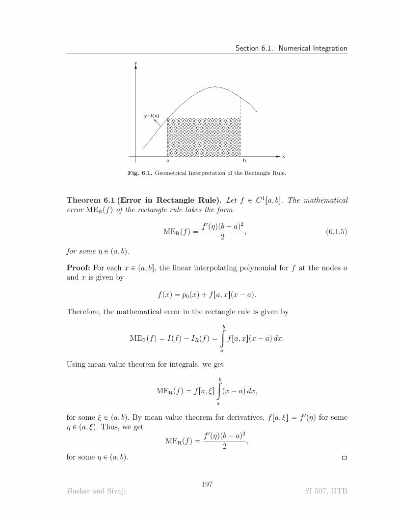
Section 6.1. Numerical Integration
�����������������������������������������������������������������������������
�����������������������������������������������������������������������������
x
y
a b
y=f(x)
Fig. 6.1. Geometrical Interpretation of the Rectangle Rule.
Theorem 6.1 (Error in Rectangle Rule). Let f P C1ra, bs. The mathematicalerror MERpfq of the rectangle rule takes the form
MERpfq “f 1pηqpb ´ aq2
2, (6.1.5)
for some η P pa, bq.
Proof: For each x P pa, bs, the linear interpolating polynomial for f at the nodes aand x is given by
fpxq “ p0pxq ` f ra, xspx ´ aq.
Therefore, the mathematical error in the rectangle rule is given by
MERpfq “ Ipfq ´ IRpfq “
bż
a
f ra, xspx ´ aq dx.
Using mean-value theorem for integrals, we get
MERpfq “ f ra, ξs
bż
a
px ´ aq dx,
for some ξ P pa, bq. By mean value theorem for derivatives, f ra, ξs “ f 1pηq for someη P pa, ξq. Thus, we get
MERpfq “f 1pηqpb ´ aq2
2,
for some η P pa, bq. [\
Baskar and Sivaji197
S I 507, IITB
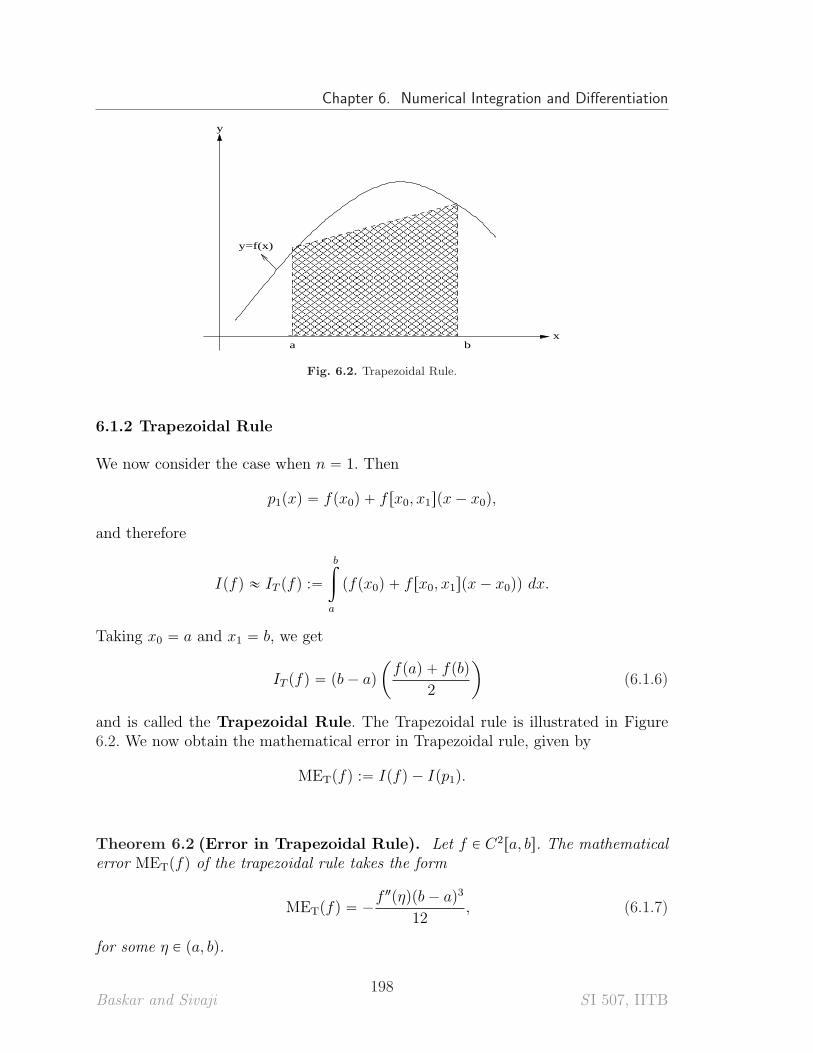
Chapter 6. Numerical Integration and Differentiation
������������������������������������������������������������������������������������������������������������������������
������������������������������������������������������������������������������������������������������������������������
x
y
a b
y=f(x)
Fig. 6.2. Trapezoidal Rule.
6.1.2 Trapezoidal Rule
We now consider the case when n “ 1. Then
p1pxq “ fpx0q ` f rx0, x1spx ´ x0q,
and therefore
Ipfq « IT pfq :“
bż
a
pfpx0q ` f rx0, x1spx ´ x0qq dx.
Taking x0 “ a and x1 “ b, we get
IT pfq “ pb ´ aq
ˆ
fpaq ` fpbq
2
˙
(6.1.6)
and is called the Trapezoidal Rule. The Trapezoidal rule is illustrated in Figure6.2. We now obtain the mathematical error in Trapezoidal rule, given by
METpfq :“ Ipfq ´ Ipp1q.
Theorem 6.2 (Error in Trapezoidal Rule). Let f P C2ra, bs. The mathematicalerror METpfq of the trapezoidal rule takes the form
METpfq “ ´f 2pηqpb ´ aq3
12, (6.1.7)
for some η P pa, bq.
Baskar and Sivaji198
S I 507, IITB
Section 6.1. Numerical Integration
Proof: We have
fpxq “ fpaq ` f ra, bspx ´ aq ` f ra, b, xspx ´ aqpx ´ bq.
Integrating over the interval ra, bs, we get
Ipfq “ IT pfq `
bż
a
f ra, b, xspx ´ aqpx ´ bqdx.
Therefore the mathematical error is given by
METpfq “ Ipfq ´ IT pfq “
bż
a
f ra, b, xspx ´ aqpx ´ bqdx. (6.1.8)
From Corollary 5.24 (Conclusion 1), we see that the function x ÞÝÑ f ra, b, xs iscontinuous. Therefore, from the mean value theorem for integrals (after noting thatpx´aqpx´bq is negative for all x P ra, bs), the expression (6.1.8) for the mathematicalerror takes the form
METpfq “ f ra, b, ηs
bż
a
px ´ aqpx ´ bqdx,
for some η P pa, bq. The formula (6.1.7) now follows from (5.3.25) and a direct evalu-ation of the above integral. [\
Example 6.3. For the function fpxq “ 1{px ` 1q, we approximate the integral
I “
1ż
0
fpxqdx,
using trapezoidal rule to get
IT pfq “1
2
ˆ
1 `1
2
˙
“3
4“ 0.75.
The true value is Ipfq “ logp2q « 0.693147. Therefore, the error is METpfq «
´0.0569. Using the formula (6.1.7), we get the bounds for METpfq as
´1
6ă METpfq ă ´
1
48
which clearly holds in the present case. [\
Baskar and Sivaji199
S I 507, IITB
Chapter 6. Numerical Integration and Differentiation
Composite Trapezoidal Rule
We can improve the approximation of trapezoidal rule by breaking the interval ra, bsinto smaller subintervals and apply the trapezoidal rule (6.1.6) on each subinterval.We will derive a general formula for this.
Let us subdivide the interval ra, bs into n equal subintervals of length
h “b ´ a
nwith endpoints of the subintervals as
xj “ a ` jh, j “ 0, 1, ¨ ¨ ¨ , n.
Then, we get
Ipfq “
bż
a
fpxqdx “
xnż
x0
fpxqdx “
n´1ÿ
j“0
xj`1ż
xj
fpxqdx.
Using Trapezoidal rule (6.1.6) on the subinterval rxj, xj`1s, we getxj`1ż
xj
fpxqdx « h
ˆ
fpxjq ` fpxj`1q
2
˙
, j “ 0, 1, ¨ ¨ ¨ , n ´ 1.
Substituting this in the above equation, we get
Ipfq « h
„
fpx0q ` fpx1q
2
ȷ
` h
„
fpx1q ` fpx2q
2
ȷ
` ¨ ¨ ¨ ` h
„
fpxn´1q ` fpxnq
2
ȷ
.
The terms on the right hand side can be combined to give the simpler formula
InT pfq :“ h
„
1
2fpx0q ` fpx1q ` fpx2q ` ¨ ¨ ¨ ` fpxn´1q `
1
2fpxnq
ȷ
. (6.1.9)
This rule is called the Composite Trapezoidal rule.
Example 6.4. Using composite trapezoidal rule with n “ 2, let us approximate theintegral
I “
1ż
0
fpxqdx,
where
fpxq “1
1 ` x.
As we have seen in Example 6.3, the true value is Ipfq “ logp2q « 0.693147. Now,the composite trapezoidal rule with x0 “ 0, x1 “ 1{2 and x2 “ 1 gives
I2T pfq « 0.70833.
Thus the error is -0.0152. Recall from Example 6.3 that with n “ 1, the trapezoidalrule gave an error of -0.0569. [\
Baskar and Sivaji200
S I 507, IITB
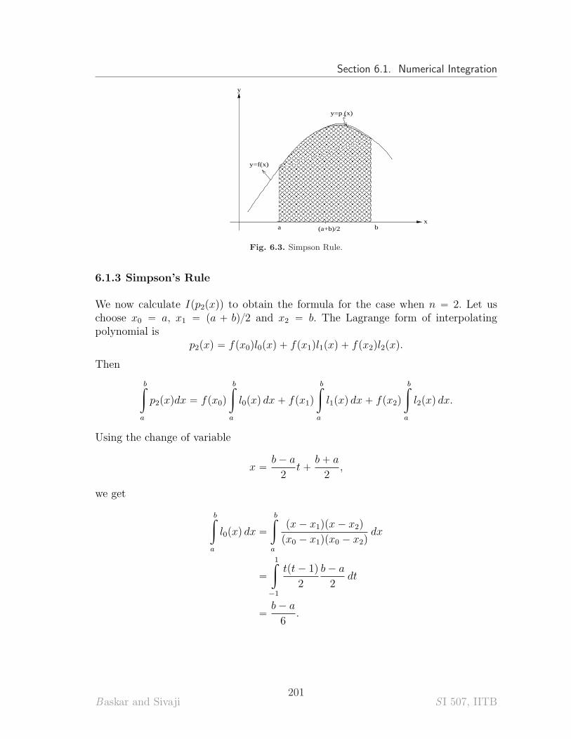
Section 6.1. Numerical Integration
������������������������������������������������������������������������������������������������������������������������
������������������������������������������������������������������������������������������������������������������������
������������������������������������������������������������������
������������������������������������������������������������������
x
y
a b(a+b)/2
y=f(x)
y=p (x)2
Fig. 6.3. Simpson Rule.
6.1.3 Simpson’s Rule
We now calculate Ipp2pxqq to obtain the formula for the case when n “ 2. Let uschoose x0 “ a, x1 “ pa ` bq{2 and x2 “ b. The Lagrange form of interpolatingpolynomial is
p2pxq “ fpx0ql0pxq ` fpx1ql1pxq ` fpx2ql2pxq.
Then
bż
a
p2pxqdx “ fpx0q
bż
a
l0pxq dx ` fpx1q
bż
a
l1pxq dx ` fpx2q
bż
a
l2pxq dx.
Using the change of variable
x “b ´ a
2t `
b ` a
2,
we get
bż
a
l0pxq dx “
bż
a
px ´ x1qpx ´ x2q
px0 ´ x1qpx0 ´ x2qdx
“
1ż
´1
tpt ´ 1q
2
b ´ a
2dt
“b ´ a
6.
Baskar and Sivaji201
S I 507, IITB
Chapter 6. Numerical Integration and Differentiation
Similarly, we can see
bż
a
l1pxq dx “4
6pb ´ aq,
bż
a
l2pxq dx “b ´ a
6.
We thus arrive at the formula
Ipfq « ISpfq :“
bż
a
p2pxqdx “b ´ a
6
"
fpaq ` 4f
ˆ
a ` b
2
˙
` fpbq
*
(6.1.10)
which is the famous Simpson’s Rule. The Simpson’s rule is illustrated in Figure6.3.
We now obtain the mathematical error in Simpson’s rule, given by,
MESpfq :“ Ipfq ´ Ipp2q.
Theorem 6.5 (Error in Simpson’s Rule). Let f P C4ra, bs. The mathematicalerror MESpfq of the Simpson’s rule takes the form
MESpfq “ ´f p4qpηqpb ´ aq5
2880, (6.1.11)
for some η P pa, bq.
Proof: Consider the collection of nodes a, pa ` bq{2, b, x in the interval ra, bs. Letx0 P ra, bs be a given point different from a, pa` bq{2, b, and x. From the fourth orderdivided difference formula, we have
f ra, pa ` bq{2, b, xs “ f rx0, a, pa ` bq{2, bs ` f rx0, a, pa ` bq{2, b, xspx ´ x0q.
The mathematical error in Simpson’s method can therefore be written as
MESpfq “
bż
a
f rx0, a, pa ` bq{2, bsϕpxqdx `
bż
a
f rx0, a, pa ` bq{2, b, xspx ´ x0qϕpxqdx,
whereϕpxq “ px ´ aqpx ´ pa ` bq{2qpx ´ bq.
A direct integration shows
Baskar and Sivaji202
S I 507, IITB
Section 6.1. Numerical Integration
bż
a
ϕpxqdx “
bż
a
px ´ aq
ˆ
x ´a ` b
2
˙
px ´ bqdx “ 0.
Thus, we have
MESpfq “
bż
a
f rx0, a, pa ` bq{2, b, xspx ´ x0qϕpxqdx,
Recall in the proof of theorem 6.2, we used mean value theorem 1.27 at this stageto arrive at the conclusion. But, in the present case, we cannot use this theorembecause the function px ´ x0qϕpxq need not be of one sign on ra, bs. However, thechoice x0 “ pa` bq{2 makes this function one signed (negative). Now using Corollary5.24 (Conclusion 1) and following the idea of the proof of Theorem 6.2, we arrive atthe formula (6.1.11) (this is left as an exercise). [\
Example 6.6. We now use the Simpson’s rule to approximate the integral
Ipfq “
1ż
0
fpxq dx,
where
fpxq “1
1 ` x.
The true value is Ipfq “ logp2q « 0.693147. Using the Simpson’s rule (6.1.10), we get
ISpfq “1
6
ˆ
1 `8
3`
1
2
˙
“25
36« 0.694444.
Therefore, the error is MESpfq « 0.001297. [\
Composite Simpson’s Rule
Let us now derive the composite Simpson’s rule. First let us subdivide the intervalra, bs into n equal parts as we discussed in composite trapezoidal rule (Subsection6.1.2). Taking a “ xi´1, b “ xi`1, (note that xi “ pxi´1 ` xi`1q{2) and xi ´ xi´1 “ hin Simpson rule, we get
ż xi`1
xi´1
fpxqdx «h
3tfpxi´1q ` 4fpxiq ` fpxi`1qu .
Summing for i “ 1, ¨ ¨ ¨ , N{2, (N even) we get
Baskar and Sivaji203
S I 507, IITB
Chapter 6. Numerical Integration and Differentiation
ż b
a
fpxqdx “
N{2ÿ
i“1
ż x2i
x2i´2
fpxqdx
«h
3
N{2ÿ
i“1
tfpx2i´2q ` 4fpx2i´1q ` fpx2iqu .
Therefore, the composite Simpson’s rule takes the form
IN{2S pfq “
h
3
«
fpx0q ` fpxNq ` 2
N{2ÿ
i“2
fpx2i´2q ` 4
N{2ÿ
i“1
fpx2i´1q
ff
. p6.12q
6.1.4 Method of Undetermined Coefficients
All the rules so far derived are of the form
Ipfq “
bż
a
fpxqdx « w0fpx0q ` w1fpx1q ` ¨ ¨ ¨ ` wnfpxnq (6.1.12)
where wi’s are weights. In deriving those rules, we have fixed the nodes x0, x1, ¨ ¨ ¨ ,xn (n “ 0 for rectangle rule, n “ 1 for trapezoidal rule and n “ 2 for Simpson’s rule),and used interpolating polynomials to obtain the corresponding weights. Instead, wemay use another approach in which for a fixed set of nodes weights are determinedby imposing the condition that the resulting rule is exact for polynomials of degreeless than or equal to n. Such a method is called the method of undeterminedcoefficients.
Example 6.7. Let us find w0, w1, and w2 such that the approximate formula
bż
a
fpxq dx « w0fpaq ` w1f
ˆ
a ` b
2
˙
` w2fpbq (6.1.13)
is exact for all polynomials of degree less than or equal to 2.
Since integral of sum of functions is the sum of the integrals of the respectivefunctions, the formula (6.1.13) is exact for all polynomials of degree less than orequal to 2 if and only if the formula (6.1.13) is exact for the polynomials 1, x, and x2.
• The condition that the formula (6.1.13) is exact for the polynomial ppxq “ 1 yields
b ´ a “
bż
a
1 dx “ w0 ` w1 ` w2
Baskar and Sivaji204
S I 507, IITB
Section 6.1. Numerical Integration
• The condition that the formula (6.1.13) is exact for the polynomial ppxq “ x yields
b2 ´ a2
2“
bż
a
x dx “ aw0 `
ˆ
a ` b
2
˙
w1 ` bw2.
• The condition that the formula (6.1.13) is exact for the polynomial ppxq “ x2
yields
b3 ´ a3
3“
bż
a
x2 dx “ a2w0 `
ˆ
a ` b
2
˙2
w1 ` b2w2
Thus, we have a linear system of three equations satisfied by w0, w1, and w2. Bysolving this system, we get
w0 “1
6pb ´ aq,
w1 “2
3pb ´ aq,
w2 “1
6pb ´ aq,
which gives us the familiar Simpson’s rule. [\
This motivates the following definition.
Definition 6.8 (Degree of Precision).
The degree of precision (also called order of exactness) of a quadrature formulais the largest positive integer n such that the formula is exact for all polynomials ofdegree less than or equal to n.
Example 6.9. Let us determine the degree of precision of Simpson’s rule. It willsuffice to apply the rule over the interval r0, 2s (in fact any interval is good enoughand we chose this interval for the sake of having easy computation).
2ż
0
dx “ 2 “2
6p1 ` 4 ` 1q,
2ż
0
xdx “ 2 “2
6p0 ` 4 ` 2q,
2ż
0
x2dx “8
3“
2
6p0 ` 4 ` 4q,
Baskar and Sivaji205
S I 507, IITB
Chapter 6. Numerical Integration and Differentiation
2ż
0
x3dx “ 4 “2
6p0 ` 4 ` 8q,
2ż
0
x4dx “32
5‰
2
6p0 ` 4 ` 16q “
20
3.
Therefore, the degree of precision of Simpson’s rule is 3. [\
Remark 6.10. In Example 6.7 we have obtained the Simpson’s rule using the methodof undetermined coefficients by requiring the exactness of the rule for polynomialsof degree less than or equal to 2, the above example shows that the rule is exact forpolynomials of degree three as well. [\
6.1.5 Gaussian Rules
In Example 6.7 we have fixed the nodes and obtained the weights in the quadraturerule (6.1.13) such that the rule is exact for polynomials of degree less than or equal to2. In general, by fixing the nodes, we can obtain the weights in (6.1.12) such that therule is exact for polynomials of degree less than or equal to n. But it is also possibleto derive a quadrature rule such that the rule is exact for polynomials of degree lessthan or equal to 2n ` 1 by choosing the n ` 1 nodes and the weights appropriately.This is the basic idea of Gaussian rules.
Let us consider the special case
1ż
´1
fpxqdx «
nÿ
i“0
wifpxiq. (6.1.14)
The weights wi and the nodes xi (i “ 0, ¨ ¨ ¨ , n) are to be chosen in such a way thatthe rule (6.1.14) is exact, that is
1ż
´1
fpxqdx “
nÿ
i“0
wifpxiq, (6.1.15)
whenever fpxq is a polynomial of degree less than or equal to 2n ` 1. Note that(6.1.15) holds for every polynomial fpxq of degree less than or equal to 2n` 1 if andonly if (6.1.15) holds for fpxq “ 1, x, x2, ¨ ¨ ¨ , x2n`1.
Case 1: (n “ 0). In this case, the quadrature formula (6.1.14) takes the form
1ż
´1
fpxqdx « w0fpx0q.
Baskar and Sivaji206
S I 507, IITB
Section 6.1. Numerical Integration
The condition (6.1.15) gives
1ż
´1
1 dx “ w0 and
1ż
´1
x dx “ w0x0.
These conditions give w0 “ 2 and x0 “ 0. Thus, we have the formula
1ż
´1
fpxqdx « 2fp0q “: IG0pfq, (6.1.16)
which is the required Gaussian rule for n “ 0.
Case 2: (n “ 1). In this case, the quadrature formula (6.1.14) takes the form
1ż
´1
fpxqdx « w0fpx0q ` w1fpx1q.
The condition (6.1.15) gives
w0 ` w1 “ 2,
w0x0 ` w1x1 “ 0,
w0x20 ` w1x
21 “
2
3,
w0x30 ` w1x
31 “ 0.
A solution of this nonlinear system is w0 “ w1 “ 1, x0 “ ´1{?3 and x1 “ 1{
?3.
This lead to the formula
1ż
´1
fpxqdx « f
ˆ
´1
?3
˙
` f
ˆ
1?3
˙
“: IG1pfq, (6.1.17)
which is the required Gaussian rule for n “ 1.
Case 3: (General). In general, the quadrature formula is given by (6.1.14), wherethere are 2pn`1q free parameters xi and wi for i “ 0, 1, ¨ ¨ ¨ , n. The condition (6.1.15)leads to the nonlinear system
nÿ
j“0
wjxij “
#
0 , i “ 1, 3, ¨ ¨ ¨ , 2n ` 12
i ` 1, i “ 0, 2, ¨ ¨ ¨ , 2n
.
These are nonlinear equations and their solvability is not at all obvious and thereforethe discussion is outside the scope of this course.
Baskar and Sivaji207
S I 507, IITB
Chapter 6. Numerical Integration and Differentiation
So far, we derived Gaussian rule for integrals over r´1, 1s. But this is not a limi-tation as any integral on the interval ra, bs can easily be transformed to an integralon r´1, 1s by using the linear change of variable
x “b ` a ` tpb ´ aq
2, ´1 ď t ď 1. (6.1.18)
Thus, we havebż
a
fpxqdx “b ´ a
2
1ż
´1
f
ˆ
b ` a ` tpb ´ aq
2
˙
dt.
Example 6.11. We now use the Gaussian rule to approximate the integral
Ipfq “
1ż
0
fpxq dx,
where
fpxq “1
1 ` x.
Note that the true value is Ipfq “ logp2q « 0.693147.
To use the Gaussian quadrature, we first need to make the linear change of variable(6.1.18) with a “ 0 and b “ 1 and we get
x “t ` 1
2, ´ 1 ď t ď 1.
Thus the required integral is
Ipfq “
1ż
0
dx
1 ` x“
1ż
´1
dt
3 ` t.
We need to take fptq “ 1{p3 ` tq in the Gaussian quadrature formula (6.1.17) andwe get
1ż
0
dx
1 ` x“
1ż
´1
dt
3 ` t« f
ˆ
´1
?3
˙
` f
ˆ
1?3
˙
« 0.692308 « IG1pfq.
Therefore, the error is Ipfq ´ IG1pfq « 0.000839. [\
Baskar and Sivaji208
S I 507, IITB
Section 6.2. Numerical Differentiation
6.2 Numerical Differentiation
The aim of this section is to obtain formulas to approximate the values of derivativesof a given function at a given point. Such a formula for the first derivative of afunction can be obtained directly using the definition of the derivative, namely, thedifference quotients of the function. This will be discussed in Subsection 6.2.1. Butthis idea cannot be adopted for higher order derivatives. Approximating formulas forderivatives can be obtained in at least two ways, namely,
(1) Methods based on Interpolation
(2) Methods based on Undetermined Coefficients
These methods are discussed in Subsections 6.2.2 and 6.2.3, respectively.
6.2.1 Approximations of First Derivative
Forward Difference Formula
The most simple way to obtain a numerical method for approximating the derivativeof a C1 function f is to use the definition of derivative
f 1pxq “ limhÑ0
fpx ` hq ´ fpxq
h.
The approximating formula can therefore be taken as
f 1pxq «fpx ` hq ´ fpxq
h“: D`
h fpxq (6.2.19)
for a sufficiently small value of h ą 0. The formula D`h fpxq is called the forward
difference formula for the derivative of f at the point x.
Theorem 6.12. Let f P C2ra, bs. The mathematical error in the forward differenceformula is given by
f 1pxq ´ D`h fpxq “ ´
h
2f2pηq (6.2.20)
for some η P px, x ` hq.
Proof: By Taylor’s theorem, we have
fpx ` hq “ fpxq ` hf 1pxq `h2
2f 2pηq (6.2.21)
for some η P px, x ` hq. Using (6.2.19) and (6.2.21), we obtain
D`h fpxq “
1
h
"„
fpxq ` hf 1pxq `h2
2f2pηq
ȷ
´ fpxq
*
“ f 1pxq `h
2f 2pηq.
This completes the proof. [\
Baskar and Sivaji209
S I 507, IITB
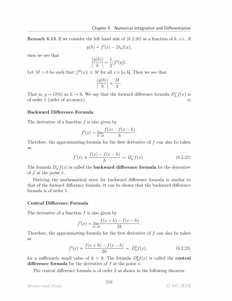
Chapter 6. Numerical Integration and Differentiation
Remark 6.13. If we consider the left hand side of (6.2.20) as a function of h, i.e., if
gphq “ f 1pxq ´ Dhfpxq,
then we see thatˇ
ˇ
ˇ
ˇ
gphq
h
ˇ
ˇ
ˇ
ˇ
“1
2|f 2pηq|.
Let M ą 0 be such that |f 2pxq| ď M for all x P ra, bs. Then we see thatˇ
ˇ
ˇ
ˇ
gphq
h
ˇ
ˇ
ˇ
ˇ
ďM
2.
That is, g “ Ophq as h Ñ 0. We say that the forward difference formula D`h fpxq is
of order 1 (order of accuracy). [\
Backward Difference Formula
The derivative of a function f is also given by
f 1pxq “ limhÑ0
fpxq ´ fpx ´ hq
h.
Therefore, the approximating formula for the first derivative of f can also be takenas
f 1pxq «fpxq ´ fpx ´ hq
h“: D´
h fpxq (6.2.22)
The formula D´h fpxq is called the backward difference formula for the derivative
of f at the point x.
Deriving the mathematical error for backward difference formula is similar tothat of the forward difference formula. It can be shown that the backward differenceformula is of order 1.
Central Difference Formula
The derivative of a function f is also given by
f 1pxq “ limhÑ0
fpx ` hq ´ fpx ´ hq
2h.
Therefore, the approximating formula for the first derivative of f can also be takenas
f 1pxq «fpx ` hq ´ fpx ´ hq
2h“: D0
hfpxq, (6.2.23)
for a sufficiently small value of h ą 0. The formula D0hfpxq is called the central
difference formula for the derivative of f at the point x.
The central difference formula is of order 2 as shown in the following theorem.
Baskar and Sivaji210
S I 507, IITB
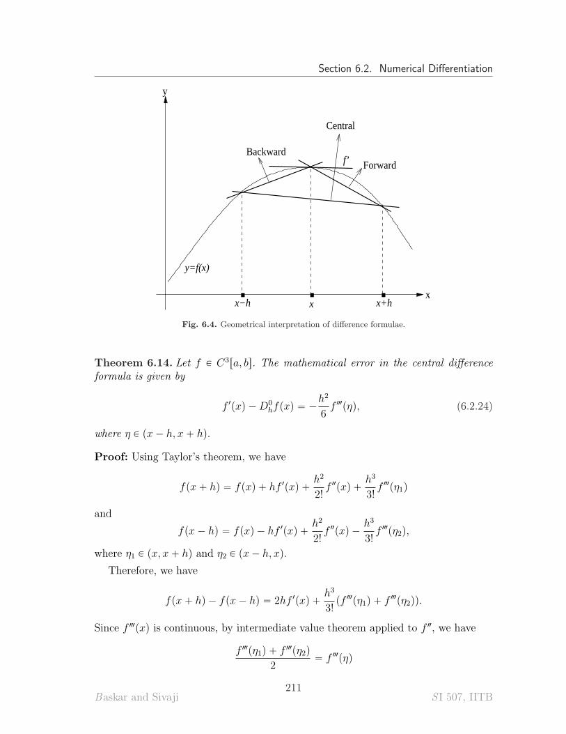
Section 6.2. Numerical Differentiation
. ..xx−h x+h
ForwardBackward
Central
x
y
y=f(x)
f’
Fig. 6.4. Geometrical interpretation of difference formulae.
Theorem 6.14. Let f P C3ra, bs. The mathematical error in the central differenceformula is given by
f 1pxq ´ D0hfpxq “ ´
h2
6f3pηq, (6.2.24)
where η P px ´ h, x ` hq.
Proof: Using Taylor’s theorem, we have
fpx ` hq “ fpxq ` hf 1pxq `h2
2!f2pxq `
h3
3!f3pη1q
and
fpx ´ hq “ fpxq ´ hf 1pxq `h2
2!f 2pxq ´
h3
3!f3pη2q,
where η1 P px, x ` hq and η2 P px ´ h, xq.
Therefore, we have
fpx ` hq ´ fpx ´ hq “ 2hf 1pxq `h3
3!pf3pη1q ` f3pη2qq.
Since f3pxq is continuous, by intermediate value theorem applied to f 2, we have
f3pη1q ` f3pη2q
2“ f3pηq
Baskar and Sivaji211
S I 507, IITB
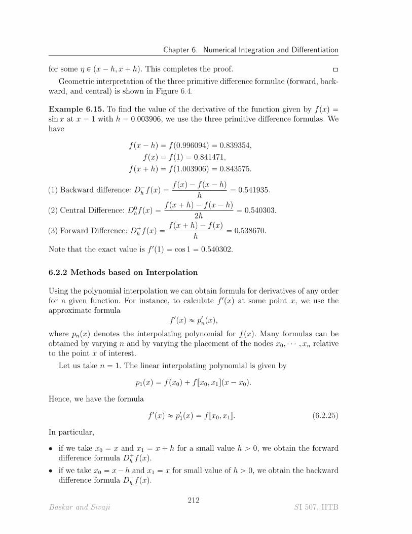
Chapter 6. Numerical Integration and Differentiation
for some η P px ´ h, x ` hq. This completes the proof. [\
Geometric interpretation of the three primitive difference formulae (forward, back-ward, and central) is shown in Figure 6.4.
Example 6.15. To find the value of the derivative of the function given by fpxq “
sinx at x “ 1 with h “ 0.003906, we use the three primitive difference formulas. Wehave
fpx ´ hq “ fp0.996094q “ 0.839354,
fpxq “ fp1q “ 0.841471,
fpx ` hq “ fp1.003906q “ 0.843575.
(1) Backward difference: D´h fpxq “
fpxq ´ fpx ´ hq
h“ 0.541935.
(2) Central Difference: D0hfpxq “
fpx ` hq ´ fpx ´ hq
2h“ 0.540303.
(3) Forward Difference: D`h fpxq “
fpx ` hq ´ fpxq
h“ 0.538670.
Note that the exact value is f 1p1q “ cos 1 “ 0.540302.
6.2.2 Methods based on Interpolation
Using the polynomial interpolation we can obtain formula for derivatives of any orderfor a given function. For instance, to calculate f 1pxq at some point x, we use theapproximate formula
f 1pxq « p1npxq,
where pnpxq denotes the interpolating polynomial for fpxq. Many formulas can beobtained by varying n and by varying the placement of the nodes x0, ¨ ¨ ¨ , xn relativeto the point x of interest.
Let us take n “ 1. The linear interpolating polynomial is given by
p1pxq “ fpx0q ` f rx0, x1spx ´ x0q.
Hence, we have the formula
f 1pxq « p11pxq “ f rx0, x1s. (6.2.25)
In particular,
• if we take x0 “ x and x1 “ x ` h for a small value h ą 0, we obtain the forwarddifference formula D`
h fpxq.
• if we take x0 “ x´h and x1 “ x for small value of h ą 0, we obtain the backwarddifference formula D´
h fpxq.
Baskar and Sivaji212
S I 507, IITB
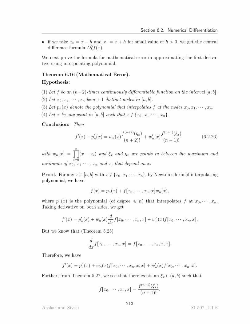
Section 6.2. Numerical Differentiation
• if we take x0 “ x ´ h and x1 “ x ` h for small value of h ą 0, we get the centraldifference formula D0
hfpxq.
We next prove the formula for mathematical error in approximating the first deriva-tive using interpolating polynomial.
Theorem 6.16 (Mathematical Error).
Hypothesis:
(1) Let f be an pn`2q-times continuously differentiable function on the interval ra, bs.
(2) Let x0, x1, ¨ ¨ ¨ , xn be n ` 1 distinct nodes in ra, bs.
(3) Let pnpxq denote the polynomial that interpolates f at the nodes x0, x1, ¨ ¨ ¨ , xn.
(4) Let x be any point in ra, bs such that x R tx0, x1 ¨ ¨ ¨ , xnu.
Conclusion: Then
f 1pxq ´ p1npxq “ wnpxq
f pn`2qpηxq
pn ` 2q!` w1
npxqf pn`1qpξxq
pn ` 1q!(6.2.26)
with wnpxq “
nź
i“0
px ´ xiq and ξx and ηx are points in between the maximum and
minimum of x0, x1 ¨ ¨ ¨ , xn and x, that depend on x.
Proof. For any x P ra, bs with x R tx0, x1 ¨ ¨ ¨ , xnu, by Newton’s form of interpolatingpolynomial, we have
fpxq “ pnpxq ` f rx0, ¨ ¨ ¨ , xn, xswnpxq,
where pnpxq is the polynomial (of degree ď n) that interpolates f at x0, ¨ ¨ ¨ , xn.Taking derivative on both sides, we get
f 1pxq “ p1npxq ` wnpxq
d
dxf rx0, ¨ ¨ ¨ , xn, xs ` w1
npxqf rx0, ¨ ¨ ¨ , xn, xs.
But we know that (Theorem 5.25)
d
dxf rx0, ¨ ¨ ¨ , xn, xs “ f rx0, ¨ ¨ ¨ , xn, x, xs.
Therefore, we have
f 1pxq “ p1npxq ` wnpxqf rx0, ¨ ¨ ¨ , xn, x, xs ` w1
npxqf rx0, ¨ ¨ ¨ , xn, xs.
Further, from Theorem 5.27, we see that there exists an ξx P pa, bq such that
f rx0, ¨ ¨ ¨ , xn, xs “f pn`1qpξxq
pn ` 1q!.
Baskar and Sivaji213
S I 507, IITB
Chapter 6. Numerical Integration and Differentiation
Using Theorem 5.27 along with the Hermite-Genocchi formula, we see that thereexists an ηx P pa, bq such that
f rx0, ¨ ¨ ¨ , xn, x, xs “f pn`2qpηxq
pn ` 2q!.
Therefore, we get
f 1pxq ´ p1npxq “ wnpxq
f pn`2qpηxq
pn ` 2q!` w1
npxqf pn`1qpξxq
pn ` 1q!
which is what we wish to show. [\
Difference formulas for higher order derivatives and their mathematical error canbe obtained similarly. The derivation of the mathematical error for the formulas ofhigher order derivatives are omitted for this course.
Example 6.17. Let x0, x1, and x2 be the given nodes. Then, the Newton’s form ofinterpolating polynomial for f is given by
p2pxq “ fpx0q ` f rx0, x1spx ´ x0q ` f rx0, x1, x2spx2 ´ px0 ` x1qx ` x0x1q.
Therefore, we take the first derivative of f as
f 1pxq « p12pxq “ f rx0, x1s ` f rx0, x1, x2sp2x ´ x0 ´ x1q.
• If we take x0 “ x ´ h, x1 “ x, and x2 “ x ` h for any given x P ra, bs, we obtainthe central difference formula D0
hpfq and the corresponding error obtained from(6.2.26) is precisely the error given in (6.2.24).
• If we take x0 “ x, x1 “ x ` h and x2 “ x ` 2h for any given x P ra, bs, we obtainthe difference formula
f 1pxq «´3fpxq ` 4fpx ` hq ´ fpx ` 2hq
2h
with mathematical error obtained using (6.2.26) as
f 1pxq ´ p12pxq “
h2
3f3pξq,
for some ξ P px, x ` 2hq. [\
Baskar and Sivaji214
S I 507, IITB
Section 6.2. Numerical Differentiation
6.2.3 Methods based on Undetermined Coefficients
Another method to derive formulas for numerical differentiation is called themethodof undetermined coefficients. The idea behind this method is similar to the onediscussed in deriving quadrature formulas.
Suppose we seek a formula for f pkqpxq that involves the nodes x0, x1, ¨ ¨ ¨ , xn.Then, write the formula in the form
f pkqpxq « w0fpx0q ` w1fpx1q ` ¨ ¨ ¨ ` wnfpxnq (6.2.27)
where wi, i “ 0, 1, ¨ ¨ ¨ , n are free variables that are obtained by imposing the conditionthat this formula is exact for polynomials of degree less than or equal to n.
Example 6.18. We will illustrate the method by deriving the formula for f2pxq atnodes x0 “ x ´ h, x1 “ x and x2 “ x ` h for a small value of h ą 0.
For a small value of h ą 0, let
f2pxq « Dp2q
h fpxq :“ w0fpx ´ hq ` w1fpxq ` w2fpx ` hq (6.2.28)
where w0, w1 and w2 are to be obtained so that this formula is exact when fpxq isa polynomial of degree less than or equal to 2. This condition is equivalent to theexactness for the three polynomials 1, x and x2.
Step 1: When fpxq “ 1 for all x. Then the formula of the form (6.2.28) is assumedto be exact and we get
w0 ` w1 ` w2 “ 0. (6.2.29)
Step 2: When fpxq “ x for all x. Then the formula of the form (6.2.28) is assumedto be exact and we get
w0px ´ hq ` w1x ` w2px ` hq “ 0.
Using (6.2.29), we get
w2 ´ w0 “ 0. (6.2.30)
Step 3: When fpxq “ x2 for all x. Then the formula of the form (6.2.28) is assumedto be exact and we get
w0px ´ hq2 ` w1x2 ` w2px ` hq2 “ 2.
Using (6.2.29) and (6.2.30), we get
w0 ` w2 “2
h2. (6.2.31)
Baskar and Sivaji215
S I 507, IITB
Chapter 6. Numerical Integration and Differentiation
Solving the linear system of equations (6.2.29), (6.2.30), and (6.2.31), we get
w0 “ w2 “1
h2, w1 “ ´
2
h2.
Substituting these into (6.2.28), we get
Dp2q
h fpxq “fpx ` hq ´ 2fpxq ` fpx ´ hq
h2, (6.2.32)
which is the required formula.
Let us now derive the mathematical error involved in this formula. For this, weuse the Taylor’s series
fpx ˘ hq “ fpxq ˘ hf 1pxq `h2
2!f 2pxq ˘
h3
3!f p3qpxq ` ¨ ¨ ¨
in (6.2.32) to get
Dp2q
h fpxq “1
h2
ˆ
fpxq ` hf 1pxq `h2
2!f 2pxq `
h3
3!f p3qpxq `
h4
4!f p4qpxq ` ¨ ¨ ¨
˙
´2
h2fpxq
`1
h2
ˆ
fpxq ´ hf 1pxq `h2
2!f2pxq ´
h3
3!f p3qpxq `
h4
4!f p4qpxq ´ ¨ ¨ ¨
˙
.
After simplification, we get
Dp2q
h fpxq “ f2pxq `h2
24rpf p4qpxq ` ¨ ¨ ¨ q ` pf p4qpxq ´ ¨ ¨ ¨ qs.
Now treating the fourth order terms on the right hand side as remainders in Taylor’sseries, we get
Dp2q
h fpxq “ f 2pxq `h2
24rf p4qpξ1q ` f p4qpξ2qs,
for some ξ1, ξ2 P px ´ h, x ` hq. Using intermediate value theorem for the functionf p4q, we get the mathematical error as
f 2pxq ´ Dp2q
h fpxq “ ´h2
12f p4qpξq (6.2.33)
for some ξ P px ´ h, x ` hq, which is the required mathematical error. [\
6.2.4 Arithmetic Error in Numerical Differentiation
Difference formulas are useful when deriving methods for solving differential equa-tions. But they can lead to serious errors when applied to function values that aresubjected to floating-point approximations. Let
Baskar and Sivaji216
S I 507, IITB
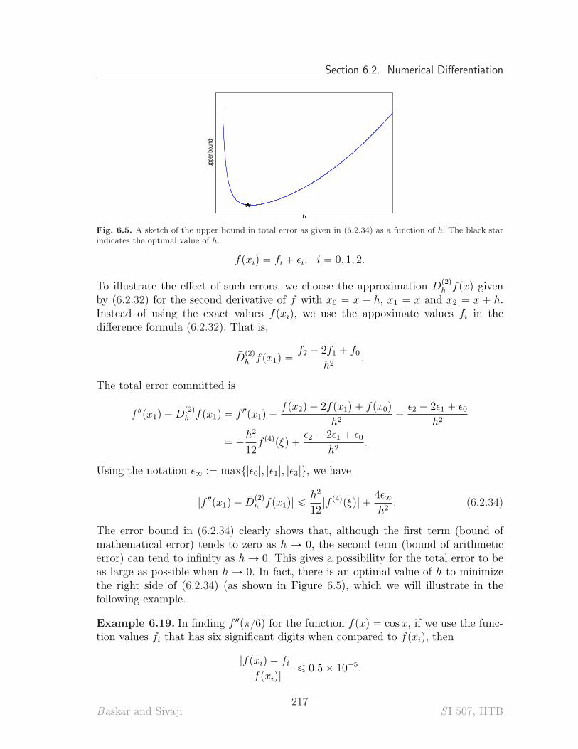
Section 6.2. Numerical Differentiation
hup
per b
ound
*
Fig. 6.5. A sketch of the upper bound in total error as given in (6.2.34) as a function of h. The black starindicates the optimal value of h.
fpxiq “ fi ` ϵi, i “ 0, 1, 2.
To illustrate the effect of such errors, we choose the approximation Dp2q
h fpxq givenby (6.2.32) for the second derivative of f with x0 “ x ´ h, x1 “ x and x2 “ x ` h.Instead of using the exact values fpxiq, we use the appoximate values fi in thedifference formula (6.2.32). That is,
Dp2q
h fpx1q “f2 ´ 2f1 ` f0
h2.
The total error committed is
f2px1q ´ Dp2q
h fpx1q “ f2px1q ´fpx2q ´ 2fpx1q ` fpx0q
h2`ϵ2 ´ 2ϵ1 ` ϵ0
h2
“ ´h2
12f p4qpξq `
ϵ2 ´ 2ϵ1 ` ϵ0h2
.
Using the notation ϵ8 :“ maxt|ϵ0|, |ϵ1|, |ϵ3|u, we have
|f 2px1q ´ Dp2q
h fpx1q| ďh2
12|f p4qpξq| `
4ϵ8
h2. (6.2.34)
The error bound in (6.2.34) clearly shows that, although the first term (bound ofmathematical error) tends to zero as h Ñ 0, the second term (bound of arithmeticerror) can tend to infinity as h Ñ 0. This gives a possibility for the total error to beas large as possible when h Ñ 0. In fact, there is an optimal value of h to minimizethe right side of (6.2.34) (as shown in Figure 6.5), which we will illustrate in thefollowing example.
Example 6.19. In finding f 2pπ{6q for the function fpxq “ cosx, if we use the func-tion values fi that has six significant digits when compared to fpxiq, then
|fpxiq ´ fi|
|fpxiq|ď 0.5 ˆ 10´5.
Baskar and Sivaji217
S I 507, IITB
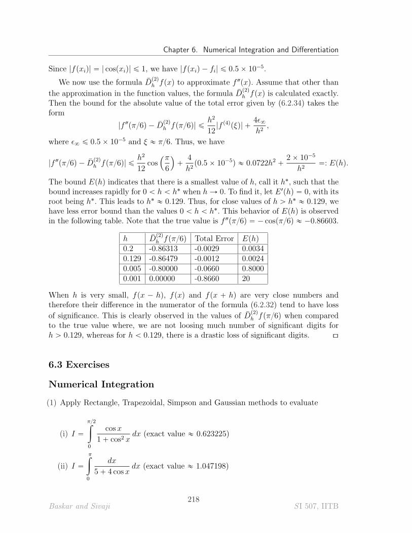
Chapter 6. Numerical Integration and Differentiation
Since |fpxiq| “ | cospxiq| ď 1, we have |fpxiq ´ fi| ď 0.5 ˆ 10´5.
We now use the formula Dp2q
h fpxq to approximate f 2pxq. Assume that other than
the approximation in the function values, the formula Dp2q
h fpxq is calculated exactly.Then the bound for the absolute value of the total error given by (6.2.34) takes theform
|f2pπ{6q ´ Dp2q
h fpπ{6q| ďh2
12|f p4qpξq| `
4ϵ8
h2,
where ϵ8 ď 0.5 ˆ 10´5 and ξ « π{6. Thus, we have
|f 2pπ{6q ´ Dp2q
h fpπ{6q| ďh2
12cos
´π
6
¯
`4
h2p0.5 ˆ 10´5q « 0.0722h2 `
2 ˆ 10´5
h2“: Ephq.
The bound Ephq indicates that there is a smallest value of h, call it h˚, such that thebound increases rapidly for 0 ă h ă h˚ when h Ñ 0. To find it, let E 1phq “ 0, with itsroot being h˚. This leads to h˚ « 0.129. Thus, for close values of h ą h˚ « 0.129, wehave less error bound than the values 0 ă h ă h˚. This behavior of Ephq is observedin the following table. Note that the true value is f2pπ{6q “ ´ cospπ{6q « ´0.86603.
h Dp2q
h fpπ{6q Total Error Ephq
0.2 -0.86313 -0.0029 0.00340.129 -0.86479 -0.0012 0.00240.005 -0.80000 -0.0660 0.80000.001 0.00000 -0.8660 20
When h is very small, fpx ´ hq, fpxq and fpx ` hq are very close numbers andtherefore their difference in the numerator of the formula (6.2.32) tend to have loss
of significance. This is clearly observed in the values of Dp2q
h fpπ{6q when comparedto the true value where, we are not loosing much number of significant digits forh ą 0.129, whereas for h ă 0.129, there is a drastic loss of significant digits. [\
6.3 Exercises
Numerical Integration
(1) Apply Rectangle, Trapezoidal, Simpson and Gaussian methods to evaluate
(i) I “
π{2ż
0
cos x
1 ` cos2 xdx (exact value « 0.623225)
(ii) I “
πż
0
dx
5 ` 4 cos xdx (exact value « 1.047198)
Baskar and Sivaji218
S I 507, IITB
Section 6.3. Exercises
(iii) I “
1ż
0
e´x2
dx (exact value « 0.746824),
(iv) I “
πż
0
sin3 x cos4 x dx (exact value « 0.114286)
(v) I “
1ż
0
p1 ` e´x sinp4xqq dx. (exact value « 1.308250)
Compute the relative error (when compared to the given exact values) in eachmethod.
(2) Write down the errors in the approximation of
1ż
0
x4dx and
1ż
0
x5dx
by the Trapezoidal rule and Simpson’s rule. Find the value of the constant C forwhich the Trapezoidal rule gives the exact result for the calculation of the integral
1ż
0
px5 ´ Cx4qdx.
(3) A function f has the values shown below:
x 1 1.25 1.5 1.75 2fpxq 10 8 7 6 5
.
(i) Use trapezoidal rule to approximateş2
1fpxq dx.
(ii) Use Simpson’s rule to approximateş2
1fpxq dx.
(iii) Use composite Simpson’s rule to approximateş2
1fpxq dx.
(4) Obtain expressions for the arithmetic error in approximating the integralşb
afpxq dx
using the trapezoidal and the Simpson’s rules. Also obtain upper bounds.
(5) Let a “ x0 ă x1 ă ¨ ¨ ¨ ă xn “ b be equally spaced nodes (i.e., xk “ x0 ` kh fork “ 1, 2, ¨ ¨ ¨ , n) in the interval ra, bs. Note that h “ pb ´ aq{n. Let f be a twicecontinuously differentiable function on ra, bs.
(i) Show that the expression for the mathematical error in approximating the
integralşb
afpxq dx using the composite trapezoidal rule, denoted by En
T pfq, isgiven by
Baskar and Sivaji219
S I 507, IITB
Chapter 6. Numerical Integration and Differentiation
EnT pfq “ ´
pb ´ aqh2
12f2pξq,
for some ξ P pa, bq.
(ii) Show that the mathematical error EnT pfq tends to zero as n Ñ 8 (one uses the
terminology Composite trapezoidal rule is convergent in such a case).
(6) Determine the minimum number of subintervals and the corresponding step sizeh so that the error for the composite trapezoidal rule is less than 5 ˆ 10´9 forapproximating the integral
ş7
2dx{x.
(7) Let a “ x0 ă x1 ă ¨ ¨ ¨ ă xn “ b be equally spaced nodes (i.e., xk “ x0 ` kh fork “ 1, 2, ¨ ¨ ¨ , n) in the interval ra, bs, and n is an even natural number. Note thath “ pb´ aq{n. Let f be a four times continuously differentiable function on ra, bs.
(i) Show that the expression for the mathematical error in approximating the
integralşb
afpxq dx using the composite Simpson rule, denoted by En
Spfq, isgiven by
EnSpfq “ ´
pb ´ aqh4
180f p4qpξq,
for some ξ P pa, bq.
(ii) Show that the mathematical error EnSpfq tends to zero as n Ñ 8 (one uses
the terminology Composite Simpson rule is convergent in such a case).
(8) Use composite Simpson’s and composite Trapezoidal rules to obtain an approxi-mate value for the improper integral
8ż
1
1
x2 ` 9dx, with n “ 4.
(9) Determine the coefficients in the quadrature formula
2hż
0
x´1{2fpxq dx « p2hq1{2pw0fp0q ` w1fphq ` w2fp2hqq
such that the formula is exact for all polynomials of degree as high as possible.What is the degree of precision?
(10) Use the two-point Gaussian quadrature rule to approximateş1
´1dx{px ` 2q and
compare the result with the trapezoidal and Simpson’s rules.
(11) Assume that xk “ x0 ` kh are equally spaced nodes. The quadrature formula
x3ż
x0
fpxqdx «3h
8pfpx0q ` 3fpx1q ` 3fpx2q ` fpx3qq
Baskar and Sivaji220
S I 507, IITB

Section 6.3. Exercises
is called the Simpson’s 38rule. Determine the degree of precision of Simpson’s 3
8
rule.
Numerical Differentiation
(12) In this problem, perform the calculations using 6-digit rounding arithmetic.
(i) Find the value of the derivative of the function fpxq “ sinx at x “ 1 using theforward, backward, and central difference formulae with h1 “ 0.015625, andh2 “ 0.000015.
(ii) Find f 1p1q directly and compare with the values obtained for each hi (i “ 1, 2).
(13) Obtain the central difference formula for f 1pxq using polynomial interpolation withnodes at x ´ h, x, x ` h, where h ą 0.
(14) Given the values of the function fpxq “ lnx at x0 “ 2.0, x1 “ 2.2 and x2 “
2.6, find the approximate value of f 1p2.0q using the method based on quadraticinterpolation. Obtain an error bound.
(15) The following data corresponds to the function fpxq “ sin x.
x 0.5 0.6 0.7fpxq 0.4794 0.5646 0.6442
Obtain the approximate value of f 1p0.5q, f 1p0.6q, and f 1p0.7q using forward, back-ward, and central difference formulae whichever are applicable. Compute the rel-ative error in all the three cases.
(16) The following data corresponds to the function fpxq “ ex ´ 2x2 ` 3x ` 1.
x 0.0 0.2 0.4fpxq 0.0 0.7414 1.3718
Obtain the approximate value of f 1p0.0q, f 1p0.2q, and f 1p0.4q using forward, back-ward, and central difference formulae whichever are applicable. Compute the rel-ative error in all the three cases.
(17) Obtain expressions for the arithmetic error in approximating the first derivativeof a function using the forward, backward, and central difference formulae.
(18) Find an approximation to f 1pxq as a formula involving fpxq, fpx ` hq, andfpx ` 2hq. Obtain an expression for the mathematical error involved in this ap-proximation.
(19) Let h ą 0. Use the method of undetermined coefficients to find a numericaldifferentiation formula for approximating f2pxq such that the formula uses valuesof the function f at each of the following sets of points:
Baskar and Sivaji221
S I 507, IITB
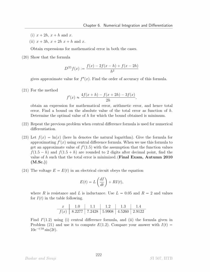
Chapter 6. Numerical Integration and Differentiation
(i) x ` 2h, x ` h and x.
(ii) x ` 3h, x ` 2h x ` h and x.
Obtain expressions for mathematical error in both the cases.
(20) Show that the formula
Dp2qfpxq :“fpxq ´ 2fpx ´ hq ` fpx ´ 2hq
h2
gives approximate value for f2pxq. Find the order of accuracy of this formula.
(21) For the method
f 1pxq «4fpx ` hq ´ fpx ` 2hq ´ 3fpxq
2h,
obtain an expression for mathematical error, arithmetic error, and hence totalerror. Find a bound on the absolute value of the total error as function of h.Determine the optimal value of h for which the bound obtained is minimum.
(22) Repeat the previous problem when central difference formula is used for numericaldifferentiation.
(23) Let fpxq “ lnpxq (here ln denotes the natural logarithm). Give the formula forapproximating f 1pxq using central difference formula. When we use this formula toget an approximate value of f 1p1.5q with the assumption that the function valuesfp1.5 ´ hq and fp1.5 ` hq are rounded to 2 digits after decimal point, find thevalue of h such that the total error is minimized. (Final Exam, Autumn 2010(M.Sc.))
(24) The voltage E “ Eptq in an electrical circuit obeys the equation
Eptq “ L
ˆ
dI
dt
˙
` RIptq,
where R is resistance and L is inductance. Use L “ 0.05 and R “ 2 and valuesfor Iptq in the table following.
x 1.0 1.1 1.2 1.3 1.4fpxq 8.2277 7.2428 5.9908 4.5260 2.9122
Find I 1p1.2q using (i) central difference formula, and (ii) the formula given inProblem (21) and use it to compute Ep1.2q. Compare your answer with Iptq “
10e´t{10 sinp2tq.
Baskar and Sivaji222
S I 507, IITB
CHAPTER 7
Numerical Ordinary Differential Equations
Consider a first order ordinary differential equation (ODE) of the form
y1 “ fpx, yq,
where y “ ypxq is an unknown variable, x P R is an independent variable and thefunction f : R ˆ R Ñ R is given. Here, we used the notation y1 :“ dy{dx. Theobjective is to find the solution y for all x P ra, bs subject to an initial condition
ypx0q “ y0, x0 P ra, bs.
We call the problem of solving the above ODE along with this initial condition, theinitial value problem.
It is well-known that there are many ODEs of physical interest that cannot besolved exactly although we know that such problems have unique solutions. If onewants the solution of such problems, then the only way is to obtain it approximately.One common way of obtaining an approximate solution to a given initial value prob-lem is to numerically compute the solution using a numerical method (or numericalscheme). In this chapter, we introduce some basic numerical methods for approxi-mating the solution of a given initial value problem.
In Section 7.1, we review the exact solvability of a given initial value problemand motivate the need of numerical methods. In Section 7.3, we introduce a basicnumerical method called Euler’s method for obtaining approximate solution of aninitial value problem and discussed the error involved in this method. We also show inthis section that the Euler method is of order 1. Modified forms of Euler method canbe obtained using numerical quadrature formulas as discussed in Section 7.4. Taylorapproximation with higher order terms can be used to obtain numerical methods ofhigher order accuracy. However, such methods involve the higher order derivativesof the unknown function and are called Taylor methods. Taylor methods are hardto implement on a computer as they involve higher order derivatives. An alternateway of achieving higher order accuracy without using higher order derivatives of theunknown function is the famous Runge-Kutta methods. Runge-Kutta method oforder 2 is derived in full detail in section 7.5 and the formula for the Runge-Kuttamethod of order 4 is stated.
Chapter 7. Numerical Ordinary Differential Equations
7.1 Review of Theory
In this section, we will discuss solving an initial value problem (IVP) for an ordinarydifferential equation. Let f be a continuous function of two variables defined on adomain D Ă R2. Let px0, y0q P D be given. The initial value problem for an ODE isgiven by
y1 “ fpx, yq, px, yq P D, (7.1.1a)
ypx0q “ y0. (7.1.1b)
The following result is concerning the equivalence of the initial value problem (7.1.1)with an integral equation.
Lemma 7.1. A continuous function y defined on an interval I containing the pointx0 is a solution of the initial value problem (7.1.1) if and only if y satisfies the integralequation
ypxq “ y0 `
ż x
x0
fps, ypsqq ds, (7.1.2)
for all x P I.
Proof: If y is a solution of the initial value problem (7.1.1), then we have
y1pxq “ fpx, ypxqq. (7.1.3)
Integrating the above equation from x0 to x yields the integral equation (7.1.2).
On the other hand let y be a solution of integral equation (7.1.2). Observe that, dueto continuity of the function x Ñ ypxq, the function s Ñ fps, ypsqq is continuous onI. Thus by fundamental theorem of integral calculus, the right hand side of (7.1.2) isa differentiable function with respect to x and its derivative is given by the functionx Ñ fpx, ypxqq, which is a continuous function. From (7.1.2), we see that y is con-tinuously differentiable and hence a direct differentiation of this equation yields theODE (7.1.1a). Evaluating (7.1.2) at x “ x0 gives the initial condition ypx0q “ y0. [\
Remark 7.2. The following are the consequences of Lemma 7.1.
• If f is a function of x only, ie., f “ fpxq, which can be integrated explicitly, thenthe integration on the right hand side of (7.1.2) can be obtained explicitely to getthe solution y of the IVP (7.1.1a) exactly.
For instance, if fpx, yq “ ex, then the solution of (7.1.1a) is ypxq “ y0 ` ex ´ ex0 .
• If f depends on y, ie., f “ fpx, yq, then (7.1.2) is an integral equation which ingeneral cannot be solved explicitly. However, there are some particular cases, forinstance when (7.1.1a) is linear, separable or exact, then we can obtain a solutionof (7.1.1a). There are certain other cases where an integral factor can be obtained
Baskar and Sivaji224
S I 507, IITB
Section 7.1. Review of Theory
through which the equation can be made exact. But, there are many ODEs forwhich none of the above mentioned methods can be used to obtain solution.
For instance, the equationy1 “ x2 ` y2
is clearly neither linear nor separable nor exact. Also any of the standard ways offinding integrating factor will not work for this equation.
When standard method cannot be used to obtain solutions exactly, several approx-imation procedures may be proposed for finding an approximate solution to theinitial value problem (7.1.1). In these procedures, one may use the ODE (7.1.1a)itself or its equivalent integral formulation (7.1.2). If we choose the ODE (7.1.1a),then the derivative may be approximated by a numerical differentiation formula.In case we choose the integral formulation (7.1.2), then we may use various nu-merical integration techniques (quadrature rules) to adopt a numerical method forapproximating the solution of the initial value problem (7.1.1). [\
Before going for a numerical method, it is important to ensure that the giveninitial value problem has a unique solution. Otherwise, we will be solving an initialvalue problem numerically, which actually does not have a solution or it may havemany solutions and we do not know which solution the numerical method obtains.Let us illustrate the non-uniqueness of solution of an initial value problem.
Example 7.3 (Peano). Let us consider the initial value problem
y1 “ 3 y2{3, yp0q “ 0. (7.1.4)
Note that ypxq “ 0 for all x P R is clearly a solution for this initial value problem.Also, ypxq “ x3 for all x P R. This initial value problem has infinite family of solutionsparametrized by c ě 0, given by
ycpxq “
#
0 if x ď c,
px ´ cq3 if x ą c,
defined for all x P R. Thus, we see that a solution to an initial value problem neednot be unique. [\
However by placing additional conditions on f , we can achieve uniqueness as statedin the following theorem. The proof of this theorem is omitted for this course.
Theorem 7.4 (Cauchy-Lipschitz-Picard’s Existence and Uniqueness Theo-rem). Let D Ď R2 be a domain and I Ă R be an interval. Let f : D Ñ R be acontinuous function. Let px0, y0q P D be a point such that the rectangle R defined by
R “ tx : |x ´ x0| ď au ˆ ty : |y ´ y0| ď bu (7.1.5)
Baskar and Sivaji225
S I 507, IITB
Chapter 7. Numerical Ordinary Differential Equations
is contained in D. Let f be Lipschitz continuous with respect to the variable y on R,i.e., there exists a K ą 0 such that
|fpx, y1q ´ fpx, y1q| ď K|y1 ´ y2| @px, y1q, px, y2q P R.
Then the initial value problem (7.1.1) has at least one solution on the interval |x ´
x0| ď δ where δ “ minta, bM
u. Moreover, the initial value problem (7.1.1) has exactlyone solution on this interval.
Remark 7.5. We state without proof that the function fpx, yq “ y2{3 in Example 7.3is not a Lipschitz function on any rectangle containing the point p0, 0q in it.
While verifying that a given function f is Lipschitz continuous is a little difficult,one can easily give a set of alternative conditions that guarantee Lipschitz continuity,and also these conditions are easy to verify.
Lemma 7.6. Let D Ď R2 be an open set and f : D Ñ R be a continuous functionsuch that its partial derivative with respect to the variable y is also continuous on D,i.e., Bf
By: D Ñ R is a continuous function. Let the rectangle R defined by
R “ tx : |x ´ x0| ď au ˆ ty : |y ´ y0| ď bu
be contained in D. Then f is Lipschitz continuous with respect to the variable y onR.
Proof: Let px, y1q, px, y2q P R. Applying mean value theorem with respect to the yvariable, we get
fpx, y1q ´ fpx, y1q “Bf
Bypx, ξqpy1 ´ y2q, (7.1.6)
for some ξ between y1 and y2. Since we are applying mean value theorem by fixingx, this ξ will also depend on x. However since Bf
By: D Ñ R is a continuous function,
it will be bounded on R. That is, there exists a number L ą 0 such that
ˇ
ˇ
ˇ
ˇ
Bf
Bypx, yq
ˇ
ˇ
ˇ
ˇ
ď L for all px, yq P R. (7.1.7)
Taking modulus in the equation (7.1.6), and using the last inequality we get
|fpx, y1q ´ fpx, y1q| “
ˇ
ˇ
ˇ
ˇ
Bf
Bypx, ξq
ˇ
ˇ
ˇ
ˇ
|py1 ´ y2q| ď L |py1 ´ y2q|.
This finishes the proof of lemma. [\
The following theorem can be used as a tool to check the existence and uniquenessof solution of a given initial value problem (7.1.1).
Baskar and Sivaji226
S I 507, IITB
Section 7.2. Discretization Notations
Corollary 7.7 (Existence and Uniqueness Theorem).
Let D Ď R2 be a domain and I Ď R be an interval. Let f : D Ñ R be a continuousfunction. Let px0, y0q P D be a point such that the rectangle R defined by
R “ tx : |x ´ x0| ď au ˆ ty : |y ´ y0| ď bu (7.1.8)
is contained in D.
If the partial derivative Bf{By is also continuous in D, then there exists a uniquesolution y “ ypxq of the initial value problem (7.1.1) defined on the interval |x´x0| ď
δ where δ “ minta, bM
u.
We state an example (without details) of an initial value problem that has a uniquesolution but the right hand side function in the differential equation is not a Lipschitzfunction. Thus this example illustrates the fact that condition of Lipschitz continuityis only a sufficient condition for uniqueness and by no means necessary.
Example 7.8. The IVP
y1 “
#
y sin 1y
if y ‰ 0
0 if y “ 0,yp0q “ 0.
has unique solution, despite the RHS not being Lipschitz continuous with respect tothe variable y on any rectangle containing p0, 0q. [\
Remark 7.9 (On Existence and Uniqueness Theorem).
(1) Though we have stated existence theorems without proof, we can confirm thattheir proofs do not give an explicit soluton of the initial value problem beingconsidered. In fact, the proofs give a sequence of functions that converge to asolution of the initial value problem.
(2) Even when the RHS of the ordinary differential equation is a function of x only,we do not have explicit solutions. For example,
y1 “ e´x2
, yp0q “ 0.
The only alternative is to approximate its solution by a numerical procedure. [\
7.2 Discretization Notations
A numerical method gives approximate value of the solution of the initial valueproblem (7.1.1) at only a discrete set of point. Thus, if we are interested in obtainingsolution for (7.1.1a) in an interval ra, bs, then we first discretize the interval as
Baskar and Sivaji227
S I 507, IITB
Chapter 7. Numerical Ordinary Differential Equations
a “ x0 ă x1 ă ¨ ¨ ¨ ă xn “ b, (7.2.9)
where each point xi, i “ 0, 1, ¨ ¨ ¨ , n is called a node. Unless otherwise stated, wealways assume that the nodes are equally spaced. That is,
xj “ x0 ` jh, j “ 0, 1, ¨ ¨ ¨n (7.2.10)
for a sufficiently small positive real number h. We use the notation for the approximatesolution as
yj “ yhpxjq « ypxjq, j “ 0, 1, ¨ ¨ ¨ , n. (7.2.11)
7.3 Euler’s Method
The most simplest numerical method for a first order ordinary differential equation(7.1.1a) is obtained by replace the first order derivative of the unknown function byits finite difference formula. Assume that we know the value of the unknown functiony at a point x “ x0. For obtaining the value of y at the point x1 “ x0 `h, we use theforward difference formula for the derivative given by
y1pxq «1
hpypx ` hq ´ ypxqq
in (7.1.1a) to get1
hpypx1q ´ ypx0qq « fpx0, ypx0qq.
This can be used to obtain the value of ypx1q in terms of x0 and ypx0q as
ypx1q « ypx0q ` hfpx0, ypx0qq.
Since we assumed that we know the value of ypx0q, the right hand side is fully knownand hence ypx1q can now be computed explicitly.
In general, if you know the value of ypxjq, j “ 0, 1, ¨ ¨ ¨ , n, we can obtain the valueof ypxj`1q by using the forward difference formula in (7.1.1a) at x “ xj to get
1
hpypxj`1q ´ ypxjqq « fpxj, ypxjqq.
Denoting the approximate value of ypxjq by yj, we can adopt the formula
yj`1 “ yj ` hfpxj, yjq, j “ 0, 1, ¨ ¨ ¨ , n ´ 1 (7.3.12)
for obtaining the values of the solution y at the discrete points xj, j “ 1, 2, ¨ ¨ ¨ , nby taking the value of y0 from the initial condition (7.1.1b). The formula (7.3.12) iscalled the forward Euler’s method.
Baskar and Sivaji228
S I 507, IITB
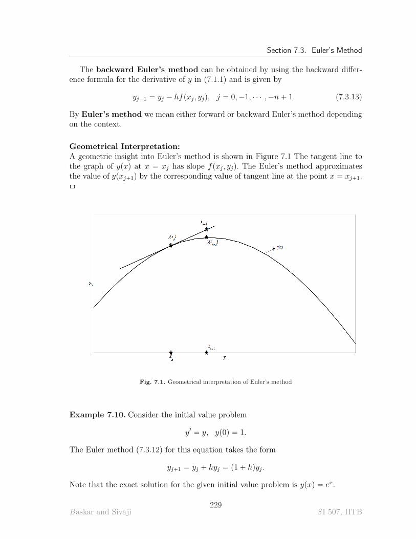
Section 7.3. Euler’s Method
The backward Euler’s method can be obtained by using the backward differ-ence formula for the derivative of y in (7.1.1) and is given by
yj´1 “ yj ´ hfpxj, yjq, j “ 0,´1, ¨ ¨ ¨ ,´n ` 1. (7.3.13)
By Euler’s method we mean either forward or backward Euler’s method dependingon the context.
Geometrical Interpretation:A geometric insight into Euler’s method is shown in Figure 7.1 The tangent line tothe graph of ypxq at x “ xj has slope fpxj, yjq. The Euler’s method approximatesthe value of ypxj`1q by the corresponding value of tangent line at the point x “ xj`1.[\
Fig. 7.1. Geometrical interpretation of Euler’s method
Example 7.10. Consider the initial value problem
y1 “ y, yp0q “ 1.
The Euler method (7.3.12) for this equation takes the form
yj`1 “ yj ` hyj “ p1 ` hqyj.
Note that the exact solution for the given initial value problem is ypxq “ ex.
Baskar and Sivaji229
S I 507, IITB
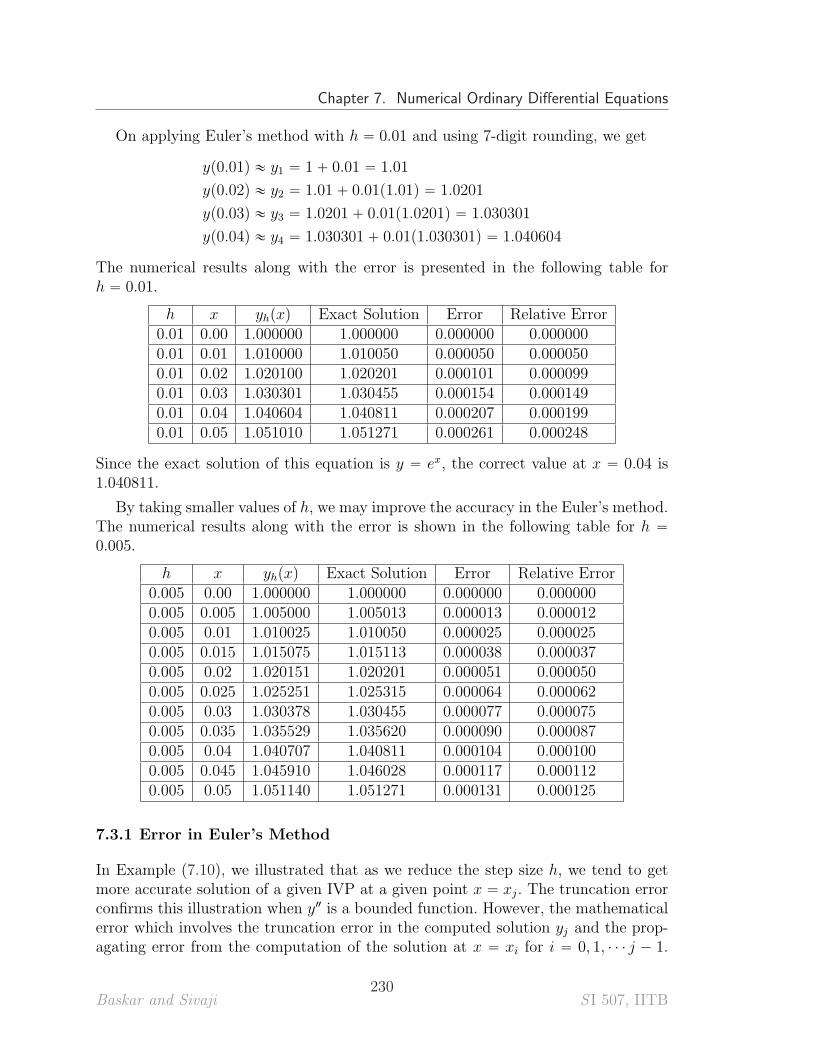
Chapter 7. Numerical Ordinary Differential Equations
On applying Euler’s method with h “ 0.01 and using 7-digit rounding, we get
yp0.01q « y1 “ 1 ` 0.01 “ 1.01
yp0.02q « y2 “ 1.01 ` 0.01p1.01q “ 1.0201
yp0.03q « y3 “ 1.0201 ` 0.01p1.0201q “ 1.030301
yp0.04q « y4 “ 1.030301 ` 0.01p1.030301q “ 1.040604
The numerical results along with the error is presented in the following table forh “ 0.01.
h x yhpxq Exact Solution Error Relative Error0.01 0.00 1.000000 1.000000 0.000000 0.0000000.01 0.01 1.010000 1.010050 0.000050 0.0000500.01 0.02 1.020100 1.020201 0.000101 0.0000990.01 0.03 1.030301 1.030455 0.000154 0.0001490.01 0.04 1.040604 1.040811 0.000207 0.0001990.01 0.05 1.051010 1.051271 0.000261 0.000248
Since the exact solution of this equation is y “ ex, the correct value at x “ 0.04 is1.040811.
By taking smaller values of h, we may improve the accuracy in the Euler’s method.The numerical results along with the error is shown in the following table for h “
0.005.
h x yhpxq Exact Solution Error Relative Error0.005 0.00 1.000000 1.000000 0.000000 0.0000000.005 0.005 1.005000 1.005013 0.000013 0.0000120.005 0.01 1.010025 1.010050 0.000025 0.0000250.005 0.015 1.015075 1.015113 0.000038 0.0000370.005 0.02 1.020151 1.020201 0.000051 0.0000500.005 0.025 1.025251 1.025315 0.000064 0.0000620.005 0.03 1.030378 1.030455 0.000077 0.0000750.005 0.035 1.035529 1.035620 0.000090 0.0000870.005 0.04 1.040707 1.040811 0.000104 0.0001000.005 0.045 1.045910 1.046028 0.000117 0.0001120.005 0.05 1.051140 1.051271 0.000131 0.000125
7.3.1 Error in Euler’s Method
In Example (7.10), we illustrated that as we reduce the step size h, we tend to getmore accurate solution of a given IVP at a given point x “ xj. The truncation errorconfirms this illustration when y2 is a bounded function. However, the mathematicalerror which involves the truncation error in the computed solution yj and the prop-agating error from the computation of the solution at x “ xi for i “ 0, 1, ¨ ¨ ¨ j ´ 1.
Baskar and Sivaji230
S I 507, IITB
Section 7.3. Euler’s Method
In addition to the mathematical error, we also have arithmetic error due to floating-point approximation in each arithmetic operation. In this section, we study the totalerror involved in forward Euler’s method. Total error involved in backward Euler’smethod can be obtained in a similar way.
Using Taylor’s theorem, write
ypxj`1q “ ypxjq ` hy1pxjq `h2
2y2pξjq
for some xj ă ξj ă xj`1. Since ypxq satisfies the ODE y1 “ fpx, ypxqq, we get
ypxj`1q “ ypxjq ` hfpxj, ypxjqq `h2
2y2pξjq.
Thus, the local truncation error in forward Euler’s method is
Tj`1 “h2
2y2pξjq, (7.3.14)
which is the error involved in obtaining the value ypxj`1q using the exact valueypxjq. The forward Euler’s method uses the approximate value yj in the formula andtherefore the finally computed value yj`1 not only involves the truncation error butalso the propagated error involved in computing yj. Thus, the local mathematicalerror in the forward Euler’s method is given by
MEpyj`1q :“ ypxj`1q ´ yj`1 “ ypxjq ´ yj ` hpfpxj, ypxjqq ´ fpxj, yjqq `h2
2y2pξjq.
Here, ypxjq ´ yj ` hpfpxj, ypxjqq ´ fpxj, yjqq is the propagated error.
The propagated error can be simplified by applying the mean value theorem tofpx, zq considering it as a functin of z:
fpxj, ypxjqq ´ fpxj, yjq “Bfpxj, ηjq
Bzrypxjq ´ yjs,
for some ηj lying between ypxjq and yj. Using this, we get the mathematical error
MEpyj`1q “
„
1 ` hBfpxj, ηjq
Bz
ȷ
MEpyjq `h2
2y2pξjq (7.3.15)
for some xj ă ξj ă xj`1, and ηj lying between ypxjq and yj.
We now assume that over the interval of interest,ˇ
ˇ
ˇ
ˇ
Bfpxj, ypxjqq
Bz
ˇ
ˇ
ˇ
ˇ
ă L, |y2pxq| ă Y,
where L and Y are fixed positive constants. On taking absolute values in (7.3.15),we obtain
Baskar and Sivaji231
S I 507, IITB
Chapter 7. Numerical Ordinary Differential Equations
|MEpyj`1q| ď p1 ` hLq|MEpyjq| `h2
2Y. (7.3.16)
Applying the above estimate recursively, we get
|MEpyj`1q| ď p1 ` hLq2|MEpyj´1q| ` p1 ` p1 ` hLqqh2
2Y
ď ¨ ¨ ¨
ď ¨ ¨ ¨
ď p1 ` hLqj`1|MEpy0q| `
´
1 ` p1 ` hLq ` p1 ` hLq2 ` ¨ ¨ ¨ ` p1 ` hLqj¯h2
2Y.
Using the formulas
(1) For any α ‰ 1,
1 ` α ` α2 ` ¨ ¨ ¨ ` αj “αj`1 ´ 1
α ´ 1
(2) For any x ě ´1,p1 ` xqN ď eNx,
in the above inequality, we have proved the following theorem.
Theorem 7.11. Let y P C2ra, bs be a solution of the IVP (7.1.1) with
ˇ
ˇ
ˇ
ˇ
Bfpx, yq
By
ˇ
ˇ
ˇ
ˇ
ă L, |y2pxq| ă Y,
for all x and y, and some constants L ą 0 and Y ą 0. The mathematical error inthe forward Euler’s method at a point xj “ x0 ` jh satisfies
|MEpyjq| ďhY
2L
`
epxn´x0qL ´ 1˘
` epxn´x0qL|ypx0q ´ y0| (7.3.17)
Example 7.12. Consider the initial value problem
y1 “ y, yp0q “ 1, x P r0, 1s.
Let us now find the upper bound for the mathematical error of forward Euler’s methodin solving this problem.
Here fpx, yq “ y. Therefore, Bf{By “ 1 and hence we can take L “ 1.
Since y “ ex, y2 “ ex and |y2pxq| ď e for 0 ď x ď 1. Therefore, we take Y “ e.
We now use the estimate (7.3.17) with x0 “ 0 and xn “ 1 to obtain
|MEpyjq| ďhe
2pe ´ 1q « 2.3354h.
Baskar and Sivaji232
S I 507, IITB
Section 7.3. Euler’s Method
Here, we assume that there is no approximation in the initial condition and thereforethe second term in (7.3.17) is zero.
To validate the upper bound obtained above, we shall compute the approximatesolution of the given IVP using forward Euler’s method. The method for the givenIVP reads
yj`1 “ yj ` hfpxj, yjq “ p1 ` hqyj.
The solution of this difference equation satisfing yp0q “ 1 is
yj “ p1 ` hqj.
Now, if h “ 0.1, n “ 10, we have yj “ p1.1q10. Therefore, the forward Euler’s methodgives yp1q « y10 « 2.5937. But the exact value is yp1q “ e « 2.71828. The error is0.12466, whereas the bound obtained from (7.3.17) was 0.2354. [\
Remark 7.13. The error bound (7.3.17) is valid for a large family of the initial valueproblems. But, it usually produces a very poor estimate due to the presence of theexponential terms. For instance, in the above example, if we take xn to be very large,then the corresponding bound will also be very large. [\
The above error analysis assumes that the numbers used are of infinite precisionand no floating point approximation is assumed. When we include the floating pointapproximation that yn “ yn ` ϵn, then the bound for total error is given in thefollowing theorem. The proof of this theorem is left as an exercise.
Theorem 7.14. Let y P C2ra, bs be a solution of the IVP (7.1.1) with
ˇ
ˇ
ˇ
ˇ
Bfpx, yq
By
ˇ
ˇ
ˇ
ˇ
ă L, |y2pxq| ă Y,
for all x and y, and some constants L ą 0 and Y ą 0. Let yj be the approximatesolution of (7.1.1) computed using the forward Euler’s method (7.3.12) with infiniteprecision and let yj be the corresponding computed value using finite digit floating-point arithmetic. If
yj “ yj ` ϵj,
then the total error TEpyjq :“ ypxjq ´ yj in forward Euler’s method at a point xj “
x0 ` jh satisfies
|TEpyjq| ď1
L
ˆ
hY
2`ϵ
h
˙
`
epxn´x0qL ´ 1˘
` epxn´x0qL|ϵ0|, (7.3.18)
where ϵ :“ maxt|ϵi|{i “ 0, 1, ¨ ¨ ¨ , nu. [\
Baskar and Sivaji233
S I 507, IITB
Chapter 7. Numerical Ordinary Differential Equations
7.4 Modified Euler’s Methods
The Euler’s method derived in the previous section can also be derived using theequivalent integral form of the IVP (7.1.1) as discussed in Lemma 7.1. Using thisintegral form in the interval rxj, xj`1s, we get
ypxj`1q “ ypxjq `
ż xj`1
xj
fps, yqds. (7.4.19)
The Euler’s method can be obtained by replacing the integral on the right hand sideby the rectangle rule.
Using the integral form in the interval rxj´1, xj`1s and using the mid-pointquadrature formula given by
ż xj`1
xj´1
fps, yqds « fpxj, yjqpxj`1 ´ xj´1q,
we get the Euler’s mid-point method
yj`1 “ yj´1 ` 2hfpxj, yjq. (7.4.20)
To compute the value of yj`1, we need to know the value of yj´1 and yj. Note thatthe above formula cannot be used to compute the value of y1. Hence, we need anothermethod to obtain y1 and then yj, for j “ 2, 3, ¨ ¨ ¨ , n can be obtained using (7.4.20).This method belongs to the class of 2-step methods.
Example 7.15. Consider the initial-value problem
y1 “ y, yp0q “ 1.
To obtain the approximate value of yp0.04q with h “ 0.01:
We first use Euler’s method to get
yp0.01q « y1 “ 1 ` 0.01 “ 1.01
Next use Euler’s mid-point method to get
yp0.02q « y2 “ y0 ` 2 ˆ h ˆ y1 “ 1 ` 2 ˆ 0.01 ˆ 1.01 “ 1.0202
yp0.03q « y3 “ y1 ` 2 ˆ h ˆ y2 “ 1.01 ` 2 ˆ 0.01 ˆ 1.0202 « 1.030404
yp0.04q « y4 “ y2 ` 2 ˆ h ˆ y3 “ 1.040808
Since the exact solution of this equation is y “ ex, the correct value at x “ 0.04 is1.040811. The error is 0.000003.
Recall the error in Euler method was 0.000199. [\
Baskar and Sivaji234
S I 507, IITB
Section 7.4. Modified Euler’s Methods
The methods derived above are explicit methods in the sense that the value ofyj`1 is computed using the known values. If we using the trapezoidal rule for theintegration on the right hand side of (7.4.19), we get
yj`1 “ yj `h
2pfpxj, yjq ` fpxj`1, yj`1qq. (7.4.21)
This method is called the Euler’s Trapezoidal method. Here, we see that theformula (7.4.21) involves an implicit relation for yj`1. Such methods are referred toas implicit methods.
Although the Euler’s Trapezoidal method gives an implicit relation for yj`1, some-times it is explicit to compute the values yj`1 as illustrated in the following example.
Example 7.16. Let us use the Euler’s trapezoidal rule with h “ 0.2 to obtain theappoximate solution of the initial value problem
y1 “ xy, yp0q “ 1.
We have y0 “ 1 and
y1 “ y0 `h
2px0y0 ` x1y1q “ 1 ` 0.1p0 ` 0.2y1q,
which gives p1 ´ 0.02qy1 “ 1, and this implies y1 « 1.0204. Similarly,
y2 “ y1 `h
2px1y1 ` x2y2q “ 1.0204 ` 0.1p0.2 ˆ 1.0204 ` 0.4y2q,
and
yp0.4q « y2 “1.0408
1 ´ 0.04« 1.0842.
[\
In general, the Euler’s trapezoidal rule gives a nonlinear equation for yj`1 as illus-trated below.
Example 7.17. Consider the initial value problem
y1 “ e´y, yp0q “ 1.
We use the Euler’s trapezoidal rule with h “ 0.2 to solve the above problem. Wehave,
y1 “ y0 `h
2pe´y0 ` e´y1q “ 1 ` 0.1pe´1 ` e´y1q,
which gives the nonlinear equation
gpy1q “ y1 ´ 0.1e´y1 ´ p1 ` 0.1e´1q “ 0,
and the solution of this equation is the approximate value of the solution ypx1q of thegiven initial value problem. [\
Baskar and Sivaji235
S I 507, IITB
Chapter 7. Numerical Ordinary Differential Equations
7.5 Runge-Kutta Methods
Although Euler’s method is easy to implement, this method is not so efficient in thesense that to get a better approximation, one needs a very small step size. One wayto get a better accuracy is to include the higher order terms in the Taylor expansionto get an approximation to y1. But the higher order terms involve higher derivativesof y. The Runge-Kutta methods attempts to obtain higher order accuracy and atthe same time avoid the need for higher derivatives, by evaluating the function fpx, yq
at selected points on each subintervals. We first derive the Runge-Kutta method oforder 2. The derivation of the Runge-Kutta method of order 4 can be done in asimilar way. So, we skip the derivation of this method and present only final formula.
7.5.1 Order Two
Let y be a solution of the ODE (7.1.1a). The Runge-Kutta method of order 2 isobtained by truncating the Taylor expansion of ypx ` hq after the quadratic term.We derive now a formula for this method. Taylor expansion of ypx` hq at the pointx upto the quadratic term is given by
ypx ` hq “ ypxq ` hy1pxq `h2
2y2pxq ` Oph3q. (7.5.22)
Since y satisfies the given ODE y1 “ fpx, yq, by differentiating this ODE with respectto x both sides gives
y2pxq “Bf
Bxpx, ypxqq ` y1pxq
Bf
Bypx, ypxqq (7.5.23)
Substituting the values of y1, y2 in (7.5.22), we get
ypx ` hq “ ypxq ` hfpx, ypxqq `h2
2
„
Bf
Bxpx, ypxqq ` fpx, ypxqq
Bf
Bypx, ypxqq
ȷ
` Oph3q.
The last equation is re-written as
ypx ` hq “ ypxq `h
2fpx, ypxqq
`h
2
„
fpx, ypxqq ` hBf
Bxpx, ypxqq ` hfpx, ypxqq
Bf
Bypx, ypxqq
ȷ
` Oph3q (7.5.24)
Taking x “ xj for j “ 0, 1, ¨ ¨ ¨ , n ´ 1 with xj`1 “ xj ` h in (7.5.24), we get
ypxj`1q “ ypxjq `h
2fpxj, ypxjqq
`h
2
„
fpxj, ypxjqq ` hBf
Bxpxj, ypxjqq ` hfpxj, ypxjqq
Bf
Bypxj, ypxjqq
ȷ
` Oph3q. (7.5.25)
Baskar and Sivaji236
S I 507, IITB
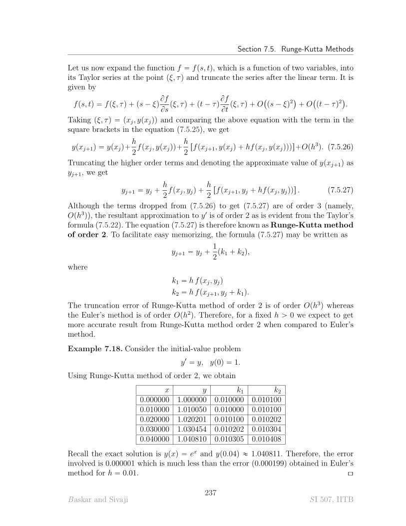
Section 7.5. Runge-Kutta Methods
Let us now expand the function f “ fps, tq, which is a function of two variables, intoits Taylor series at the point pξ, τq and truncate the series after the linear term. It isgiven by
fps, tq “ fpξ, τq ` ps ´ ξqBf
Bspξ, τq ` pt ´ τq
Bf
Btpξ, τq ` O
`
ps ´ ξq2˘
` O`
pt ´ τq2˘
.
Taking pξ, τq “ pxj, ypxjqq and comparing the above equation with the term in thesquare brackets in the equation (7.5.25), we get
ypxj`1q “ ypxjq`h
2fpxj, ypxjqq`
h
2rfpxj`1, ypxjq ` hfpxj, ypxjqqqs`Oph3q. (7.5.26)
Truncating the higher order terms and denoting the approximate value of ypxj`1q asyj`1, we get
yj`1 “ yj `h
2fpxj, yjq `
h
2rfpxj`1, yj ` hfpxj, yjqqs . (7.5.27)
Although the terms dropped from (7.5.26) to get (7.5.27) are of order 3 (namely,Oph3q), the resultant approximation to y1 is of order 2 as is evident from the Taylor’sformula (7.5.22). The equation (7.5.27) is therefore known asRunge-Kutta methodof order 2. To facilitate easy memorizing, the formula (7.5.27) may be written as
yj`1 “ yj `1
2pk1 ` k2q,
where
k1 “ h fpxj, yjq
k2 “ h fpxj`1, yj ` k1q.
The truncation error of Runge-Kutta method of order 2 is of order Oph3q whereasthe Euler’s method is of order Oph2q. Therefore, for a fixed h ą 0 we expect to getmore accurate result from Runge-Kutta method order 2 when compared to Euler’smethod.
Example 7.18. Consider the initial-value problem
y1 “ y, yp0q “ 1.
Using Runge-Kutta method of order 2, we obtain
x y k1 k20.000000 1.000000 0.010000 0.0101000.010000 1.010050 0.010000 0.0101000.020000 1.020201 0.010100 0.0102020.030000 1.030454 0.010202 0.0103040.040000 1.040810 0.010305 0.010408
Recall the exact solution is ypxq “ ex and yp0.04q « 1.040811. Therefore, the errorinvolved is 0.000001 which is much less than the error (0.000199) obtained in Euler’smethod for h “ 0.01. [\
Baskar and Sivaji237
S I 507, IITB
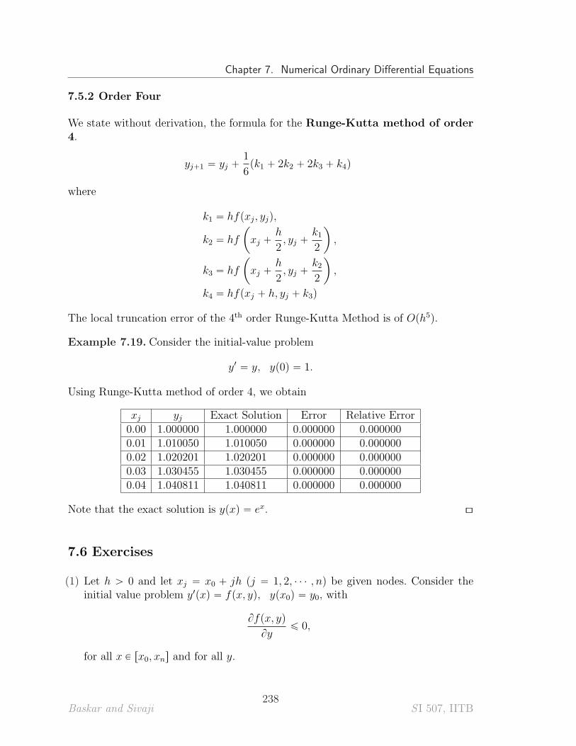
Chapter 7. Numerical Ordinary Differential Equations
7.5.2 Order Four
We state without derivation, the formula for the Runge-Kutta method of order4.
yj`1 “ yj `1
6pk1 ` 2k2 ` 2k3 ` k4q
where
k1 “ hfpxj, yjq,
k2 “ hf
ˆ
xj `h
2, yj `
k12
˙
,
k3 “ hf
ˆ
xj `h
2, yj `
k22
˙
,
k4 “ hfpxj ` h, yj ` k3q
The local truncation error of the 4th order Runge-Kutta Method is of Oph5q.
Example 7.19. Consider the initial-value problem
y1 “ y, yp0q “ 1.
Using Runge-Kutta method of order 4, we obtain
xj yj Exact Solution Error Relative Error0.00 1.000000 1.000000 0.000000 0.0000000.01 1.010050 1.010050 0.000000 0.0000000.02 1.020201 1.020201 0.000000 0.0000000.03 1.030455 1.030455 0.000000 0.0000000.04 1.040811 1.040811 0.000000 0.000000
Note that the exact solution is ypxq “ ex. [\
7.6 Exercises
(1) Let h ą 0 and let xj “ x0 ` jh (j “ 1, 2, ¨ ¨ ¨ , n) be given nodes. Consider theinitial value problem y1pxq “ fpx, yq, ypx0q “ y0, with
Bfpx, yq
Byď 0,
for all x P rx0, xns and for all y.
Baskar and Sivaji238
S I 507, IITB
Section 7.6. Exercises
(i) Using error analysis of the Euler’s method, show that there exists an h ą 0such that
|en| ď |en´1| `h2
2f 2pξq for some ξ P pxn´1, xnq,
where en “ ypxnq ´ yn with yn obtained using Euler method.
(ii) Applying the conclusion of (i) above recursively, prove that
|en| ď |e0| ` nh2 Y where Y “1
2max
x0ďxďxn
|y2pxq|. p˚˚q
(2) The solution of the initial value problem
y1pxq “ λypxq ` cos x ´ λ sinx, yp0q “ 0
is ypxq “ sinx. For λ “ ´20, find the approximate value of yp3q using the Euler’smethod with h “ 0.5. Compute the error bound given in (˚˚), and Show that theactual absolute error exceeds the computed error bound given in (˚˚). Explainwhy it does not contradict the validity of (˚˚).
(3) Derive the backward Euler’s method for finding the approximate value of ypxnq forsome xn ă 0, where y satisfies the initial value problem y1pxq “ fpx, yq, yp0q “ y0.
(4) Consider the initial value problem y1 “ ´2y, 0 ď x ď 1, yp0q “ 1.
(i) Find an upper bound on the error in approximating the value of yp1q computedusing the Euler’s method (at x “ 1) in terms of the step size h.
(ii) For each h, solve the difference equation which results from the Euler’s method,and obtain an approximate value of yp1q.
(iii) Find the error involved in the approximate value of yp1q obtained in (ii) aboveby comparing with the exact solution.
(iv) Compare the error bound obtained in (i) with the actual error obtained in (iii)for h “ 0.1, and for h “ 0.01.
(v) If we want the absolute value of the error obtained in (iii) to be at most0.5 ˆ 10´6, then how small the step size h should be?
(5) Consider the initial value problem y1 “ xy, yp0q “ 1. Estimate the error involvedin the approximate value of yp1q computed using the Euler’s method (with infiniteprecision) with step size h “ 0.01.
(6) Find an upper bound for the propagated error in Euler method (with infiniteprecision) with h “ 0.1 for solving the initial value problem y1 “ y, yp0q “ 1, inthe interval
(i) r0, 1s and
Baskar and Sivaji239
S I 507, IITB
Chapter 7. Numerical Ordinary Differential Equations
(ii) r0, 5s.
(7) For each n P N, write down the Euler’s method for the solution of the initial valueproblem y1 “ y, yp0q “ 1 on the interval r0, 1s with step size h “ 1{n. Let theresulting approximation to yp1q be denoted by αn. Show using limiting argument(without using the error bound) that αn Ñ yp1q as n Ñ 8.
(8) In each of the following initial value problems, use the Euler’s method, Runge-Kutta method of order 2 and 4 to find the solution at the specified point withspecified step size h:
(i) y1 “ x ` y; yp0q “ 1. Find yp0.2q (For the Euler’s method take h “ 0.1 andfor other methods, take h “ 0.2). The exact solution is ypxq “ ´1 ´ x ` 2ex.
(ii) y1 “ 2 cos x ´ y, yp0q “ 1. Find yp0.6q (For the Euler’s method take h “ 0.1and for other methods, take h “ 0.2) The exact solution is ypxq “ sin x`cosx.
(9) Use the Euler’s, Runge-Kutta methods of order 2 and 4 to solve the IVP y1 “
0.5px´ yq for all x P r0, 3s with initial condition yp0q “ 1. Compare the solutionsfor h “ 1, 0.5, 0.25, 0.125 along with the exact solution ypxq “ 3e´x{2 ` x ´ 2.
(10) Show that the Euler’s and Runge-Kutta methods fail to determine an approxima-tion to the non-trivial solution of the initial value problem y1 “ yα, 0 ă α ă 1,yp0q “ 0. Note that the ODE is in separable form and hence a non-trivial solutionto initial value problem can be found analytically.
(11) Write the formula using the Euler’s method for approximating the solution to theinitial value problem
y1 “ x2 ` y2, ypx0q “ y0
at the point x “ x1 with h “ x0 ´ x1 ą 0. Find the approximate value y1 of thesolution to this initial value problem at the point x1 when x0 “ 0, y0 “ 1, andh “ 0.25. Find a bound for the truncation error in obtaining y1.
(12) Using the Gaussian rule determine a formula for solving the initial value problem
y1 “ e´x2
, ypx0q “ y0.
in the formyj`1 “ yj´1 ` h
´
e´pxj´ h?
3q2
` e´pxj` h?
3q2¯
when the nodes are equally spaced with spacing h “ xj`1 ´ xj, j P Z. (h ą 0).Let x0 “ 0, and y0 “ 1. Using the method derived above, obtain approximatevalues of yp´0.1q and yp0.1q. (Mid-sem Exam, Spring 2012)
Baskar and Sivaji240
S I 507, IITB
Index
l1 norm, 73n-digit floating-point number, 302-step method, 234
Absolute error, 36Arithmetic error, 29
in interpolating polynomial, 174, 177
Backward difference, 210Backward substitution, 54, 59, 64Big Oh, 21, 22Binary representation, 30Bisection method, 120Bounded sequence, 8Bracketing method, 120
Central difference, 210Chebyshev nodes, 183Cholesky’s factorization, 70Chopping a number, 34Closed domain method, 120Composite
Simpson’s rule, 204trapezoidal rule, 200
Condition numberof a function, 44of a matrix, 77
Continuity of a function, 11Continuous function, 11Contraction map, 143Convergent sequence, 8Crout’s factorization, 70Cubic spline, 185
Data, 160Decimal representation, 30Decreasing sequence, 8Degree of precision, 205Derivative of a function, 12Diagonally dominant matrix, 84Difference
backward, 210central, 210forward, 209
Differentiable function, 12Direct method, 51, 53, 80Divided difference, 167
higher-order formula, 168symmetry, 168
Dominant eigenvalue, 93Doolittle’s factorization, 65Double precision, 34
EigenvaluePower method, 95dominant, 93
Error, 36absolute, 36arithmetic, 29floating-point, 42in Euler’s method, 230in interpolating polynomial, 174arithmetic, 174, 177mathematical, 174, 175total, 174
in iterative procedure, 84in rectangle rule, 196in Simpson’s rule, 202in trapezoidal rule, 198mathematical, 29percentage, 36propagated, 42propagation of, 40relative, 36relative total, 42residual, 88total, 29, 42truncation, 18, 37
Euclidean norm, 73Euler’s method
forward, 228, 229mid-point, 234
Index
modified, 234trapezoidal, 235
Exact arithmetic, 34Explicit method, 235Exponent, 30
Faber’s theorem, 181First mean value theorem for integrals, 15Fixed point, 140
iteration method, 141Floating-point
approximation, 33error, 42representation, 30
Forwarddifference, 209elimination, 54, 59substitution, 63
Gauss-Seidel method, 86Gaussian
rules, 206Gaussian elimination method
modified, 56Naive, 53operations count, 59
Gerschgorin’scircle theorem, 107disk, 108
Hermite-Gennochi formula, 171Hilbert matrix, 78
Ill-conditionedfunction evaluation, 45
Ill-conditioned matrix, 78Implicit method, 235Increasing sequence, 8Infinite norm, 176Infinite precision, 34Initial
condition, 223value problem, 223
Intermediate value theorem, 12Interpolating function, 159Interpolating polynomials; convergence, 181Interpolation, 159
condition, 160error, 174arithmetic, 174, 177mathematical, 174, 175total, 174
linear polynomial, 165piecewise polynomial, 183polynomial, 160, 162existence and uniqueness, 160Lagrange’s form, 164
Newton’s form, 166quadratic polynomial, 165spline, 185
Iterativemethods, 119
Iterative method, 51, 80fixed-point, 141Gauss-Seidel, 86Jacobi, 81refinement, 90residual corrector, 90
Jacobi method, 81
Lagrange’sform of interpolating polynomial, 164polynomial, 163
Limitof a function, 10of a sequence, 8left-hand, 9of a function, 11right-hand, 10
Linear systemdirect method, 51, 53Gaussian elimination method, 53, 56iterative method, 51LU factorization, 64Thomas method, 60
Little oh, 21, 22LU factorization/decomposition, 64
Cholesky’s, 70Crout’s, 70Doolittle’s, 65
Machine epsilon, 36Mantissa, 30Mathematical error, 29
in central difference formula, 211in difference formulas, 213in Euler’s method, 231in forward difference formula, 209in interpolating polynomial, 174, 175
Matrix norm, 74maximum-of-column-sums, 76maximum-of-row-sums, 75spectral, 76subordinate, 75
Maximum norm, 73Maximum-of-column-sums norm, 76Maximum-of-row-sums norm, 75Mean value theorem
derivative, 14, 17integrals, 15
Mid-point rule, 196, 234Modified Gaussian elimination method, 56Monotonic sequence, 8
Baskar and Sivaji242
S I 507, IITB
Section Index
Naive Gaussian elimination method, 53Natural spline, 186Newton’s
divided difference, 167form of interpolating polynomial, 166
Newton-Cotes formula, 196Newton-Raphson method, 135Nodes, 160, 228
Chebyshev, 183Nonlinear equation, 119
bisection method, 120Newton-Raphson method, 135regula-falsi method, 125secant method, 133
Norminfinite, 176matrix, 74maximum-of-column-sums, 76maximum-of-row-sums, 75spectral, 76subordinate, 75
vector, 73l1, 73Euclidean, 73maximum, 73
Numerical integration, 195Gaussian rule, 206mid-point, 196Newton-Cotes, 196rectangle, 196Simpson’s rule, 202, 205trapezoidal, 198
OhBig and Little, 21, 22
Open domain methods, 120Optimum bound, 109Order
of accuracy, 210of convergence, 23
Order of exactness, 205Ordinary differential equation, 223Overflow, 31
Percentage error, 36Piecewise polynomial interpolation, 183Polynomial interpolation, 160, 162
existence and uniqueness, 160Lagrange’s form, 164Newton’s form, 166piecewise linear, 183
Positive definite matrix, 70Power method, 94, 95Precision, 33
degree of, 205double, 34infinite, 34
Principal minors, 65leading, 65
Principal sub-matrix, 65Propagated error, 42
in Euler’s method, 231Propagation of error, 40
Quadrature, 195Gaussian, 206mid-point, 196Newton-Cotes, 196rectangle, 196Simpson’s, 202, 205trapezoidal, 198
Quadrature mid-point, 234
Radix, 30Rate of convergence, 23Rectangle rule, 196Regula-falsi method, 125Relative error, 36Relative total error, 42remainder estimate, 18Remainder term
in Taylor’s formula, 16Residual
error, 88vector, 88
Residual corrector method, 90Residual error, 132Rolle’s theorem, 13Rounding a number, 34Runge
function, 180phenomenon, 180
Runge-Kutta methodorder 2, 237order 4, 238
Sandwich theorem, 8, 11Secant method, 133Second mean value theorem for integrals, 15Self map, 142Sequence, 7
bounded, 8convergent, 8decreasing, 8increasing, 8limit, 8monotonic, 8
Sign, 30Significant digits, 37
loss of, 39number of, 38
Simpson’s rule, 202, 205composite, 204
Spectral norm, 76
Baskar and Sivaji243
S I 507, IITB
Index
Spline interpolation, 185cubic, 185natural, 186
Stabilityin function evaluation, 46
Stable computation, 46Stopping criteria
method for nonlinear equations, 91, 131Subordinate norms, 75
Taylor’sformula, 17polynomial, 16series, 19Theorem, 37theorem, 16
Thomas method, 60Total Error
in polynomial interpolation, 179Total error, 29, 42
in interpolating polynomial, 174Trapezoidal rule, 198
composite, 200Triangle inequality, 73, 74Truncation error, 18, 37
in Euler’s method, 231
Underflow, 31Undetermined coefficients
differentiation, 215integration, 204
Unit round, 36Unstable computation, 46
Vector norm, 73l1, 73Euclidean, 73maximum, 73
Weights, 196Well-conditioned
function evaluation, 45Well-conditioned matrix, 78Wilkinson’s example, 92
Baskar and Sivaji244
S I 507, IITB