Introduction to Modal Logics(Draft)

Stefan Wolfl

July 22, 2015

2

Contents

1 From Propositional to Modal Logic 51.1 Propositional logic . . . . . . . . . . . . . . . . . . . . . . . . . . . . . . . . 51.2 A simple modal logic . . . . . . . . . . . . . . . . . . . . . . . . . . . . . . . 7

2 Modal Language, Frames, and Models 132.1 Relational structures . . . . . . . . . . . . . . . . . . . . . . . . . . . . . . . 132.2 Modal languages . . . . . . . . . . . . . . . . . . . . . . . . . . . . . . . . . 162.3 Relational models and satisfaction . . . . . . . . . . . . . . . . . . . . . . . . 192.4 Constructing models . . . . . . . . . . . . . . . . . . . . . . . . . . . . . . . 242.5 Translating modal logic into first-order logic . . . . . . . . . . . . . . . . . . . 272.6 Consequence relation and compactness . . . . . . . . . . . . . . . . . . . . . . 292.7 Expressiveness . . . . . . . . . . . . . . . . . . . . . . . . . . . . . . . . . . 31

3 Normal Modal Logics, Frame Classes, and Definability 393.1 Normal modal logics . . . . . . . . . . . . . . . . . . . . . . . . . . . . . . . 393.2 Kripke frames and definability . . . . . . . . . . . . . . . . . . . . . . . . . . 413.3 Proving theorems . . . . . . . . . . . . . . . . . . . . . . . . . . . . . . . . . 453.4 Soundness and completeness . . . . . . . . . . . . . . . . . . . . . . . . . . . 483.5 Canonical frames, definability, and compactness . . . . . . . . . . . . . . . . . 533.6 The modal logic S4 . . . . . . . . . . . . . . . . . . . . . . . . . . . . . . . . 563.7 The modal logic S5 . . . . . . . . . . . . . . . . . . . . . . . . . . . . . . . . 583.8 The modal logic KL . . . . . . . . . . . . . . . . . . . . . . . . . . . . . . . 60

4 Decidability and Complexity 654.1 Finite Model Property . . . . . . . . . . . . . . . . . . . . . . . . . . . . . . . 654.2 Filtration . . . . . . . . . . . . . . . . . . . . . . . . . . . . . . . . . . . . . 684.3 Complexity . . . . . . . . . . . . . . . . . . . . . . . . . . . . . . . . . . . . 70

5 Decision Procedures 815.1 A tableaux procedure for K(m) . . . . . . . . . . . . . . . . . . . . . . . . . . 815.2 Tableaux procedures for other modal logics . . . . . . . . . . . . . . . . . . . 875.3 Optimization techniques . . . . . . . . . . . . . . . . . . . . . . . . . . . . . 89

3

4

1 From Propositional to Modal Logic

1.1 Propositional logic

Let P be a set of propositional variables. The language LPL(P) has the following list of symbolsas alphabet: variables from P, the logical symbols ⊥, >, ¬, →, ∧, ∨, ↔, and brackets. Theset of LPL(P)-formulae, then, is defined as the smallest set of words over this alphabet thatcontains ⊥, >, each p ∈ P, and is closed under the formation rule: If ϕ and ψ are formulae,then so are ¬ϕ , (ϕ ∧ψ), (ϕ ∨ψ), and (ϕ→ψ). We may express this in an abbreviated manneras:

ϕ ::=⊥ | > | p | ¬ϕ | (ϕ ∧ϕ′) | (ϕ ∨ϕ

′) | (ϕ→ϕ′) | (ϕ ↔ ϕ

′)

— where p ranges over P. Propositional variables are also referred to as atomic formulae.LPL(P) will also denote the set of LPL(P)-formulae, and for abbreviation we will use the nota-tions LPL, L(P), or simply L if this is understood from the context.

The semantics of propositional logic is defined in terms of truth assignments. A truth assign-ment is simply a function V : P→{0,1}, i.e., V assigns to each atomic formula a truth value 0(“false”) or 1 (“true”). Given a truth assignment V , the satisfaction relation is then defined asfollows:

V 6|=⊥V |=>V |= p ⇐⇒ V (p) = 1

V |= ¬ϕ ⇐⇒ V 6|= ϕ

V |= ϕ ∧ψ ⇐⇒ V |= ϕ and V |= ψ

V |= ϕ ∨ψ ⇐⇒ V |= ϕ or V |= ψ

V |= ϕ→ψ ⇐⇒ V 6|= ϕ or V |= ψ

V |= ϕ ↔ ψ ⇐⇒ V |= ϕ iff V |= ψ

Definition 1.1. An LPL-formula ϕ is satisfiable if there exists a truth assignment V such thatV |= ϕ . It is valid if for each truth assignment V , it holds V |= ϕ and contingent if it is neithervalid nor unsatisfiable. Two formulae ϕ and ψ are (logically) equivalent (or: PL-equivalent)if they are satisfied in the same sets of truth assignments. Given a set of LPL-formulae, Σ, aformulae ϕ , and a truth assignment V , we write: V |= Σ if V satisfies each ϕ ∈ Σ, and Σ |= ϕ

if for each truth assignment V with V |= Σ, it holds that V |= ϕ . ϕ is then said to be a PL-consequence of Σ.

We remark that most of these concepts also make sense if we restrict them to classes of truthassignments: Let C be a class of truth assignments (on the same set of propositional variablesP). Then ϕ is called C -satisfiable if ϕ is satisfied in some V chosen from C , C -valid if ϕ issatisfied in each V in C , etc.

From these definitions, it is clear that for all formulae ϕ and ψ , (ϕ∧ψ) is equivalent to ¬(ϕ→¬ψ) and (ϕ ∨ψ) equivalent to (¬ϕ→ψ), etc. That is, one can drop, for example, ∧, ∨, ↔,

5

>, and ⊥ from the alphabet and instead use them as abbreviations in the meta-language:

(ϕ ∧ψ) := ¬(ϕ→¬ψ)

(ϕ ∨ψ) := (¬ϕ→ψ)

(ϕ ↔ ψ) := ((ϕ→ψ)∧ (ψ→ϕ))

> := (p0→ p0)

⊥ := ¬>

where p0 is a fixed chosen propositional variable in P.

A complete system of truth-functional connectives is any set of truth-functional connectives inwhich each truth-functional connective of arbitrary arity is definable. Examples include thesystems {¬,→}, {¬,∧}, {¬,∨}, and {⊥,→}. In what follows we will often switch betweendifferent such complete systems as appropriate in the respective context. Most of the times,however, we will stick to the system {¬,→}.

For truth assignments V and V ′, we say that V and V ′ coincide on Q⊆ P (and write V =Q V ′)if for each q ∈ Q, V (q) =V ′(q).

Lemma 1.1 (Coincidence Lemma). Let V and V ′ be truth assignments that coincide on Q⊆ P.Then for each formula ϕ in which only propositional variables from Q occur, it holds:

V |= ϕ ⇐⇒ V ′ |= ϕ. C

Definition 1.2. A substitution is a map σ : P→ LPL. Each substitution can be extended to afunction ·σ : LPL→ LPL via the following recursive definition:

pσ := σ(p)

(¬ϕ)σ := ¬ϕσ

(ϕ→ψ)σ := ϕσ→ψ

σ

. . .

If a substitution σ simply “replaces” each occurrence of variable p by a formula ϕ , we simplywrite ψ[p/ϕ] instead of ψσ . Analogously, we will use the notation ψ[p1/ϕ1, . . . , pk/ϕk] toindicate that the variables p1, . . . , pn are simultaneously replaced by ϕ1, . . . ,ϕn, respectively.

Lemma 1.2 (Substitution Lemma). Let σ be a substitution and V be a truth assignment. DefineV σ by V σ (p) = 1 if and only if V |= σ(p) for p ∈ P. Then for each formula ϕ ,

V σ |= ϕ ⇐⇒ V |= ϕσ . C

Lemma 1.3 (Interpolation Theorem). For any LPL-formulae ϕ and ψ with ϕ |= ψ , there existsan LPL-formula χ such that

(a) in χ only such propositional variables occur that occur in both ϕ and ψ , and

(b) it holds ϕ |= χ and χ |= ψ . C

In the situation of the lemma the formula χ is called an interpolant of ϕ and ψ . Actually, theproof requires that one of the symbols ⊥ and/or > are in the language LPL. Otherwise, theclaim only holds true for ϕ |= ψ , where at least one propositional variable occurs in both ϕ andψ .

6

Definition 1.3. The degree of an LPL-formula ϕ , degϕ , is the number of logical connectivesoccurring in ϕ . The length of ϕ is the number of alphabet symbols occurring ϕ . Note that bothnotions depend on the chosen system of truth-functional connectives.

Remark 1.1. It is an NP-complete problem (referred to as SAT) to decide for a given LPL-formula ϕ whether it is satisfiable. The problem is also NP-complete if satisfiability is to bechecked for propositional formulae in conjunctive normal form (CNF). A formula is in CNF ifit is a conjunction of disjunctions of literals (a literal is a negated or unnegated atomic formula),i.e., the formula has the form

n∧i=1

mi∨ji

li ji , (CNF)

where li ji is of the form p or ¬p for some propositional variable p. Accordingly, the problemto decide whether a given formula is valid is co-NP-complete.

1.2 A simple modal logic

In what follows we will introduce a very simple “modal logic”. Again let P be a set of atomicpropositions (or propositional variables). The language L�(P) has the following list of sym-bols as alphabet: propositions of P, the logical symbols ¬,→, and �, and brackets. The set ofL�(P)-formulae, then, is defined as follows:

ϕ ::= p | ¬ϕ | (ϕ→ϕ′) | �ϕ

— where p ranges over P. L�(P) will also denote the set of L�(P)-formulae, and for abbrevi-ation we will use the notations L�, L�(P), or simply L if this is understood.

On the basis of the connectives of L�(P), we can define:

♦ϕ := ¬�¬ϕ

(ϕ �→ ψ) :=�(ϕ→ψ)

Definition 1.4. A valuation model is a non-trivial family V = {Vs}s∈S of truth assignments ofL� (“non-trivial” means that S is a non-empty set). The elements of S are referred to as states(or possible worlds). V can be thought of as a function (called P-valuation on S) V : S→ 2P,i.e., it assigns to each state s in S a (possibly empty) set of propositional variables (namelythose that are true in Vs).

Given a valuation model V , we define a satisfaction relation as follows:

V |=s p ⇐⇒ p ∈V (s)

V |=s ¬ϕ ⇐⇒ V 6|=s ϕ

V |=s ϕ→ψ ⇐⇒ V 6|=s ϕ or V |=s ψ

V |=s �ϕ ⇐⇒ V |=s′ ϕ, for each s′ ∈ S

By this definition and the definition of ♦, the truth condition for ♦ϕ is then given by:

V |=s ♦ϕ ⇐⇒ V |=s ¬�¬ϕ

⇐⇒ V 6|=s �¬ϕ

⇐⇒ V 6|=s′ ¬ϕ, for some s′ ∈ S

⇐⇒ V |=s′ ϕ, for some s′ ∈ S

7

p,q, r,¬s

s0

¬p,q, r,¬s

s1

p, q,¬r,¬s

s2

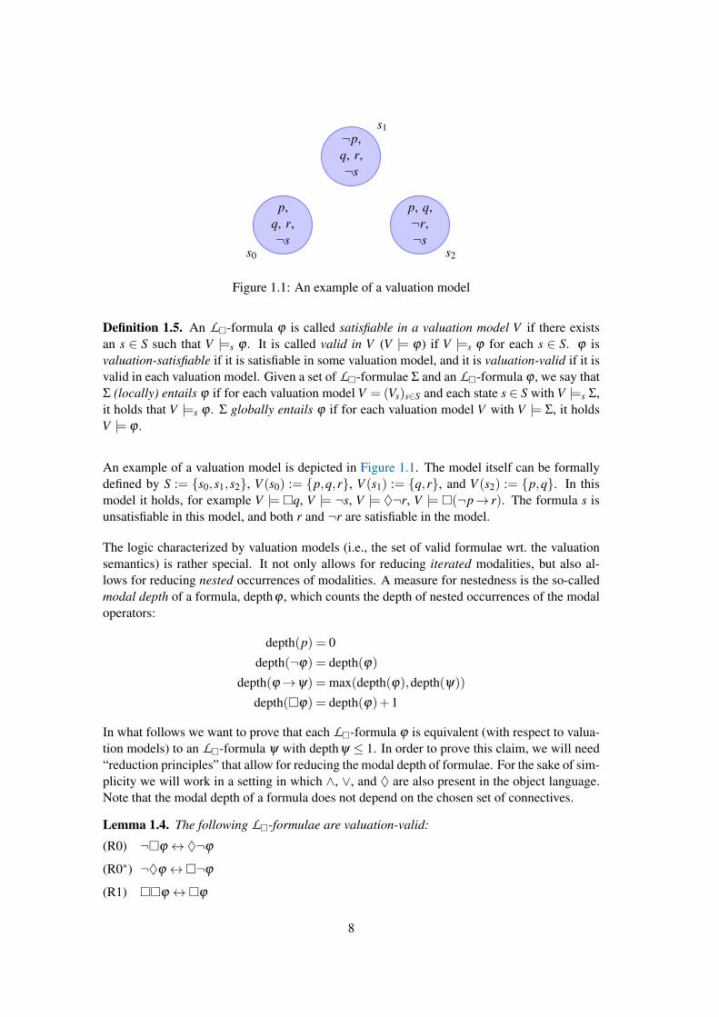
Figure 1.1: An example of a valuation model

Definition 1.5. An L�-formula ϕ is called satisfiable in a valuation model V if there existsan s ∈ S such that V |=s ϕ . It is called valid in V (V |= ϕ) if V |=s ϕ for each s ∈ S. ϕ isvaluation-satisfiable if it is satisfiable in some valuation model, and it is valuation-valid if it isvalid in each valuation model. Given a set of L�-formulae Σ and an L�-formula ϕ , we say thatΣ (locally) entails ϕ if for each valuation model V = (Vs)s∈S and each state s ∈ S with V |=s Σ,it holds that V |=s ϕ . Σ globally entails ϕ if for each valuation model V with V |= Σ, it holdsV |= ϕ .

An example of a valuation model is depicted in Figure 1.1. The model itself can be formallydefined by S := {s0,s1,s2}, V (s0) := {p,q,r}, V (s1) := {q,r}, and V (s2) := {p,q}. In thismodel it holds, for example V |= �q, V |= ¬s, V |= ♦¬r, V |= �(¬p→ r). The formula s isunsatisfiable in this model, and both r and ¬r are satisfiable in the model.

The logic characterized by valuation models (i.e., the set of valid formulae wrt. the valuationsemantics) is rather special. It not only allows for reducing iterated modalities, but also al-lows for reducing nested occurrences of modalities. A measure for nestedness is the so-calledmodal depth of a formula, depthϕ , which counts the depth of nested occurrences of the modaloperators:

depth(p) = 0

depth(¬ϕ) = depth(ϕ)

depth(ϕ→ψ) = max(depth(ϕ),depth(ψ))

depth(�ϕ) = depth(ϕ)+1

In what follows we want to prove that each L�-formula ϕ is equivalent (with respect to valua-tion models) to an L�-formula ψ with depthψ ≤ 1. In order to prove this claim, we will need“reduction principles” that allow for reducing the modal depth of formulae. For the sake of sim-plicity we will work in a setting in which ∧, ∨, and ♦ are also present in the object language.Note that the modal depth of a formula does not depend on the chosen set of connectives.

Lemma 1.4. The following L�-formulae are valuation-valid:

(R0) ¬�ϕ ↔ ♦¬ϕ

(R0∗) ¬♦ϕ ↔�¬ϕ

(R1) ��ϕ ↔�ϕ

8

(R1∗) ♦♦ϕ ↔ ♦ϕ

(R2) ♦�ϕ ↔�ϕ

(R2∗) �♦ϕ ↔ ♦ϕ

(R3) �(ϕ ∧ψ)↔ (�ϕ ∧�ψ)

(R3∗) ♦(ϕ ∨ψ)↔ (♦ϕ ∨♦ψ)

(R4) �(ϕ ∨�ψ)↔ (�ϕ ∨�ψ)

(R4∗) ♦(ϕ ∧♦ψ)↔ (♦ϕ ∧♦ψ)

(R5) �(ϕ ∨♦ψ)↔ (�ϕ ∨♦ψ)

(R5∗) ♦(ϕ ∧�ψ)↔ (♦ϕ ∧�ψ) C

Theorem 1.5. Each L�-formula ϕ is equivalent (with respect to valuation models) to an L�-formula ψ with depthψ ≤ 1.

Proof. For the proof let ϕ be a formula with depthϕ ≥ 2. We present a procedure that syntac-tically transforms ϕ into an equivalent formula with modal depth at most 1.

1. Rewrite ϕ in such a way that only ¬, �, ♦, ∧, and ∨ occur in it, i.e., we replace in ϕ

each subformula of the form (ψ→ψ ′) by (¬ψ ∨ψ ′) and each subformula of the form(ψ ↔ ψ ′) by ((¬ψ ∨ψ ′)∧ (ψ ∨¬ψ ′)).

2. Rewrite ϕ such that the negation symbol only occurs in front of propositional variables.For this, until ϕ can not be further modified,

a) apply the de Morgan laws, i.e., replace subformulae of ϕ of the form ¬(ψ ∧ψ ′) by(¬ψ ∨¬ψ ′) and subformulae of the form ¬(ψ ∨ψ ′) by (¬ψ ∧¬ψ ′);

b) apply rules (R0) and (R0∗): replace subformulae of the form ¬�ψ by ♦¬ψ andsubformulae of the form ¬♦ψ by �¬ψ;

c) absorb iterated negations (¬¬ϕ ↔ ϕ);

d) absorb iterated modalities where possible (by applying rules (R1), (R1∗), (R2), and(R2∗)).

3. Distribute modalities in front of disjunctions and conjunctions, where possible. For this,as long as the depth of ϕ is greater than 1,

a) apply rules (R3) and (R3∗) on suitable subformulae of ϕ;

b) apply rules (R4), (R4∗), (R5), and (R5∗) on suitable subformulae of ϕ (this reducesthe modal depth);

c) absorb iterated modalities where possible (by applying rules (R1), (R1∗), (R2), and(R2∗));

d) apply the PL commutativity, associativity, or distributivity laws if necessary.

In fact, if after step (2.) ϕ has modal depth greater than 2, then ϕ has a subformula ψ of theform �ψ ′ or ♦ψ ′, where depthψ ′ = depthϕ − 1 and ψ ′ is a conjunction or a disjunction offormulae.

Case 1: Assume ψ =�ψ ′.

9

Case 1.1: If ψ ′ is a conjunction of formulae ψ ′1,ψ′2, then by (R3) �ψ ′ is replaced by

(�ψ ′1∧�ψ ′2).

Case 1.2: If ψ ′ is a disjunction of formulae ψ ′1 and ψ ′2 and one of these has the form�τ

or ♦τ , then we can apply (R4) or (R5), thus reducing the depth of ψ ′.

Case 1.3: If ψ ′ is a disjunction ψ ′1∨ψ ′2, but neither of the formulae ψ ′1,ψ′2 has the form

�τ or ♦τ , then one of it must be a disjunction or a conjunction of formulae. Inthe first case apply the associative law and in the second case apply the distributivelaw to the formula ψ ′. Note that after applying the distributivity law we obtain aformula that can be handled as in Case 1.1.

Case 2: ψ = ♦ψ ′. The procedure is analogous to that of case 1.

Since all the transformations applied in this procedure result in equivalent formulae, the result-ing formula is equivalent to the input formula. C

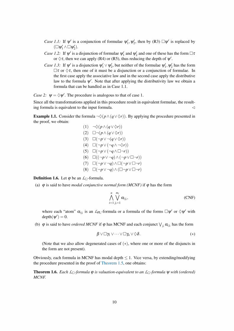
Example 1.1. Consider the formula ¬♦(p∧ (q∨♦r)). By applying the procedure presented inthe proof, we obtain:

(1) ¬♦(p∧ (q∨♦r))(2) �¬(p∧ (q∨♦r))(3) �(¬p∨¬(q∨♦r))(4) �(¬p∨ (¬q∧¬♦r))(5) �(¬p∨ (¬q∧�¬r))(6) �((¬p∨¬q)∧ (¬p∨�¬r))(7) �(¬p∨¬q)∧�(¬p∨�¬r)(8) �(¬p∨¬q)∧ (�¬p∨�¬r)

Definition 1.6. Let ϕ be an L�-formula.

(a) ϕ is said to have modal conjunctive normal form (MCNF) if ϕ has the form

n∧i=1

mi∨ji=1

αi ji , (CNF)

where each “atom” αi ji is an LPL-formula or a formula of the forms �ψ ′ or ♦ψ ′ withdepth(ψ ′) = 0.

(b) ϕ is said to have ordered MCNF if ϕ has MCNF and each conjunct∨

ji αi ji has the form

β ∨�γ1∨·· ·∨�γn∨♦δ . (∗)

(Note that we also allow degenerated cases of (∗), where one or more of the disjuncts inthe form are not present).

Obviously, each formula in MCNF has modal depth ≤ 1. Vice versa, by extending/modifyingthe procedure presented in the proof of Theorem 1.5, one obtains:

Theorem 1.6. Each L�-formula ϕ is valuation-equivalent to an L�-formula ψ with (ordered)MCNF.

10

Proof. By the procedure presented in the proof of Theorem 1.5, we obtain a formula withmodal depth ≤ 1 that is a disjunction of conjunctions (or a conjunction of disjunctions) offormulae that are of modal depth 0 or have the form�γ or ♦γ , where γ is a formula with modaldepth 0. In the first case we apply the distributive and (if necessary) the associative laws toobtain a formula in MCNF. Obviously, if a formula ϕ has MCNF, it can easily be transformedinto an equivalent formula with ordered MCNF by applying the theorem (♦δ1∨♦δ2)↔♦(δ1∨δ2). C

Example 1.2. As an example consider the formula�(♦p→ p)→�(p→�p). We first reducethis formula to a formula with modal depth 1:

(1) ¬�(¬♦p∨ p)∨�(¬p∨�p)(2) ♦(♦p∧¬p)∨�(¬p∨�p)(3) (♦p∧♦¬p)∨ (�¬p∨�p)

From this one obtains MCNF by the distributivity laws:

(4) (♦p∨�¬p∨�p)∧ (♦¬p∨�¬p∨�p)

By simply reordering (4) we get a formula in ordered MCNF

(5) (�¬p∨�p∨♦p)∧ (�¬p∨�p∨♦¬p)

Using this result, we can now introduce a test for deciding whether a given formula ϕ isvaluation-valid. Thereto, we can assume that ϕ already has ordered MCNF. Then, by defi-nition, ϕ is a conjunction of formulae that have the form

β ∨�γ1∨·· ·∨�γn∨♦δ , (∗)

where all formulae β ,γ1, . . . ,γn,δ have modal depth 0. Consider then the disjunctions

β ∨δ , γ1∨δ , . . . , γn∨δ , (∗∗)

which are obviously formulae of PL. A formula of form (∗) is said to pass the disjunction testif at least one of the disjunctions in (∗∗) is valid in PL and a conjunction of such formulae issaid to pass the disjunction test if each of its conjuncts passes it.In the example presented above, formula (5) has two conjuncts and we have to test both ofthem. In the disjunction test for the first conjunct, �¬p∨�p∨♦p, we have to test whetherone of the disjunctions

(6) ¬p∨ p, p∨ p

is PL-valid, which of course is the case. For the second conjunct, �¬p∨�p∨♦¬p, thedisjunction test gives

(7) ¬p∨¬p, p∨¬p

and here the second formula is obviously PL-valid. Thus, both conjuncts pass the disjunctiontest, and hence so does (5).

Lemma 1.7. Let ϕ be an L�-formula of the form (∗). Then ϕ passes the disjunction test if andonly if ϕ is valid in each valuation model.

11

Proof. Observation: Given a valuation model V = {Vs}s∈S, for each s ∈ S and each formula ψ

with depthψ = 0, we have:V |=s ψ ⇐⇒ Vs |= ψ.

Let now ϕ be a formula of the form (∗) that passes the disjunction test. Then at least one of thedisjunctions in (∗∗) is PL-valid. We have to show that ϕ is valid in each valuation model. Forproof by contradiction, assume that this is not the case. Then there exists a valuation model{Vs}s and a state s0 such that V 6|=s0 ϕ . That is, V 6|=s0 β , V 6|=s0 ♦δ , and for each 1 ≤ i ≤ n,V 6|=s0 �γi. Thus V 6|=s δ for each s ∈ S. Hence (by the observation), Vs0 6|= β ∨ δ . Moreover,for each i there is a state si such that Vsi 6|= γi∨δ — in contradiction to the assumption that β ∨δ

or one of the γi∨δ is PL-valid.For the other direction, let ϕ be a formula of the form (∗) that does not pass the disjunctiontest. That is, none of the disjuncts β ∨δ , γ1∨δ , . . . , γn∨δ is PL-valid. We have to show thatϕ is not valid in the sense of the valuation semantics (i.e., it needs to be shown that there existsa valuation model and a state in that model that falsifies ϕ). Since each of these disjunctions isnot valid in PL, there exist truth assignments V0, . . . ,Vn such that V0 6|= β ∨ δ and Vi 6|= γi ∨ δ ,for each 1 ≤ i ≤ n. Consider the valuation model V = {Vi}i∈{0,...,n}. Then it follows: V 6|=0 β ,V 6|=i γi for each 1≤ i≤ n, and V 6|=i δ for each 0≤ i≤ n. Thus, V 6|=0 ϕ . C

Since a conjunction of formulae is valuation-valid if and only if each of the conjuncts is so, weobtain:

Theorem 1.8. An L�-formula is valuation-valid if and only if it is valuation-equivalent to aformula in ordered MCNF that passes the disjunction test. C

In fact, what we have done is the following: we have “reduced” the problem of testing thevalidity of L�-formulae to the problem of testing a suitable set of LPL-formulae for validity.Since transforming a formula into ordered MCNF can be done by an algorithm (note thatby applying the distributive laws, the length of the formula may increase exponentially) andsince testing PL-validity is decidable, testing L�-formulae for validity is a decidable decisionproblem.

Theorem 1.9. The problem of testing a L�-formula for validity (in terms of valuation seman-tics) is decidable. C

Bibliographic remarks

There are a series of text books that introduce into classic propositional and classical first-order logics (Ebbinghaus et al., 2007; Schoning, 2000; Kutschera and Breitkopf, 2007). Thereare also quite good introductions to modal logics. To list some of them (some are somewhatadvanced): Hughes and Cresswell (1996) – a classical, comprehensive book on modal logicsthat supersedes two previous books (Hughes and Cresswell, 1985, 1990) – , Chellas (1980),Chagrov and Zakharyaschev (1997), Kutschera (1976), Kracht (1999), Gabbay et al. (2003) (avery good introduction to multi-dimensional modal logics) and Blackburn et al. (2002), whichis in most parts the basis of these lecture notes.In this chapter, section 1.2 (specifically the parts on modal conjunctive normal forms and thedecision procedure based on the disjunction test) draws much from Hughes and Cresswell(1996), chapter 5.

12

2 Modal Language, Frames, and Models

In this section we describe basic modal-logical concepts in a rather general setting. We intro-duce multi-modal languages with modal operators of arbitrary arity and introduce the relationalsemantics for these languages. Moreover we discuss different concrete examples of such modallogics, namely temporal logic, epistemic logic, and dynamic logic. However, we start by defin-ing relational structures and discussing different types of such structures that will be topic inlater sections.

2.1 Relational structures

A relation on a set S is any subset R ⊆ Sn for a fixed natural number n (the arity of R). Sincerelations are sets, we can apply set-theoretical operations on them, for example, if R is an n-ary relation, then its complement Sn \R is an n-ary relation as well. And if R1 and R2 aresuch relation, then so are R1∩R2 and R1∪R2. If σ is a permutation of {1, . . . ,n}, then Rσ :={(s1, . . . ,sn)∈ Sn : (sσ−1(1), . . . ,sσ−1(n))∈R} is an n-ary relation. Instead of s=(s1, . . . ,sn)∈R,we often simply write Rs or Rs1 . . .sn. If R is a binary relation, we will use infix notation s1 Rs2instead of writing Rs1s2.

Often we will be interested in binary relations (also called dyadic relations) and their properties.

Definition 2.1. A binary relation R on S is called

(a) reflexive if s R s for each s ∈ S;

(b) irreflexive if s R s for no s ∈ S;

(c) serial if for each s ∈ S there is an s′ ∈ S such that s R s′;

(d) symmetric if s2 R s1 whenever s1 R s2;

(e) asymmetric if there are no s1,s2 ∈ S such that s1 R s2 and s2 R s1;

(f) antisymmetric if for all s1,s2 ∈ S with s1 R s2 and s2 R s1, s1 = s2;

(g) transitive if for all s1,s2,s3 ∈ S with s1 R s2 and s2 R s3, s1 R s3;

(h) Euclidean if for all s1,s2,s3 ∈ S with s1 R s2 and s1 R s3, s2 R s3;

(i) universal for all s1,s2 ∈ S, s1 R s2.

(j) connected if for all s1,s2 ∈ S, s1 R s2 or s2 R s1;

(k) weakly connected if for all s1,s2,s3 ∈ S with s1 R s2 and s1 R s3, s2 R s3 or s3 R s2;

(l) well-founded if there is no infinite chain . . .s2 R s1 R s0 in S (see Definition 2.2);

(m) functional if for all s1,s2,s3 ∈ S with s1 R s2 and s1 R s3, s2 = s3.

(n) convergent if for all s1,s2,s3 ∈ S with s1 R s2 and s1 R s3, there exists an s4 ∈ S with s2 R s4and s3 R s4.

Lemma 2.1.(a) If R is reflexive and Euclidean, then it is symmetric and transitive.

(b) If R is symmetric and transitive, then it is Euclidean.

(c) If R is serial, symmetric, transitive, then it is reflexive.

13

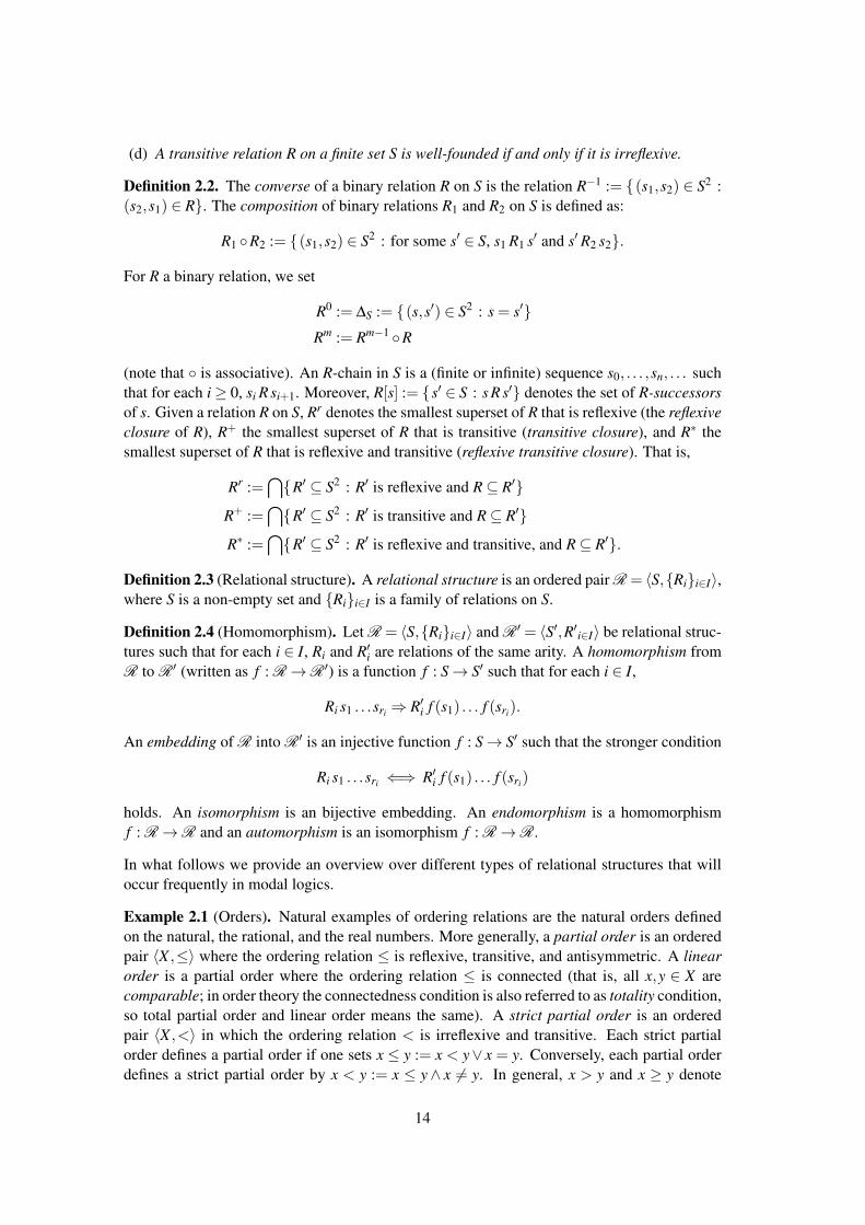
(d) A transitive relation R on a finite set S is well-founded if and only if it is irreflexive.

Definition 2.2. The converse of a binary relation R on S is the relation R−1 := {(s1,s2) ∈ S2 :(s2,s1) ∈ R}. The composition of binary relations R1 and R2 on S is defined as:

R1 ◦R2 := {(s1,s2) ∈ S2 : for some s′ ∈ S, s1 R1 s′ and s′ R2 s2}.

For R a binary relation, we set

R0 := ∆S := {(s,s′) ∈ S2 : s = s′}Rm := Rm−1 ◦R

(note that ◦ is associative). An R-chain in S is a (finite or infinite) sequence s0, . . . ,sn, . . . suchthat for each i≥ 0, si R si+1. Moreover, R[s] := {s′ ∈ S : s R s′} denotes the set of R-successorsof s. Given a relation R on S, Rr denotes the smallest superset of R that is reflexive (the reflexiveclosure of R), R+ the smallest superset of R that is transitive (transitive closure), and R∗ thesmallest superset of R that is reflexive and transitive (reflexive transitive closure). That is,

Rr :=⋂{R′ ⊆ S2 : R′ is reflexive and R⊆ R′}

R+ :=⋂{R′ ⊆ S2 : R′ is transitive and R⊆ R′}

R∗ :=⋂{R′ ⊆ S2 : R′ is reflexive and transitive, and R⊆ R′}.

Definition 2.3 (Relational structure). A relational structure is an ordered pair R = 〈S,{Ri}i∈I〉,where S is a non-empty set and {Ri}i∈I is a family of relations on S.

Definition 2.4 (Homomorphism). Let R = 〈S,{Ri}i∈I〉 and R ′ = 〈S′,R′i∈I〉 be relational struc-tures such that for each i ∈ I, Ri and R′i are relations of the same arity. A homomorphism fromR to R ′ (written as f : R→R ′) is a function f : S→ S′ such that for each i ∈ I,

Ri s1 . . .sri ⇒ R′i f (s1) . . . f (sri).

An embedding of R into R ′ is an injective function f : S→ S′ such that the stronger condition

Ri s1 . . .sri ⇐⇒ R′i f (s1) . . . f (sri)

holds. An isomorphism is an bijective embedding. An endomorphism is a homomorphismf : R→R and an automorphism is an isomorphism f : R→R.

In what follows we provide an overview over different types of relational structures that willoccur frequently in modal logics.

Example 2.1 (Orders). Natural examples of ordering relations are the natural orders definedon the natural, the rational, and the real numbers. More generally, a partial order is an orderedpair 〈X ,≤〉 where the ordering relation ≤ is reflexive, transitive, and antisymmetric. A linearorder is a partial order where the ordering relation ≤ is connected (that is, all x,y ∈ X arecomparable; in order theory the connectedness condition is also referred to as totality condition,so total partial order and linear order means the same). A strict partial order is an orderedpair 〈X ,<〉 in which the ordering relation < is irreflexive and transitive. Each strict partialorder defines a partial order if one sets x ≤ y := x < y∨ x = y. Conversely, each partial orderdefines a strict partial order by x < y := x ≤ y∧ x 6= y. In general, x > y and x ≥ y denote

14

s0

s1

s2

s3

α

α

β β

ββ

γ

γ

s0

s1

s2

s3

α

α

β β

β β

ββ

β β

γ

γ

Figure 2.1: Transition systems

the converse relations of x < y and x ≤ y, respectively. If for all x,y ∈ X , either x < y, x = y,or y < x holds (trichotomy condition), a strict partial order is said to be a strict linear order.There are even weaker ordering concepts: In a preoder the ordering is just assumed to bereflexive and transitive. Thus partial orders are those preorders in which the ordering relationis antisymmetric. A weak order is a total preorder and a strict weak order is a strict partialorder in which the incomparability relation is transitive.

Example 2.2 (Equivalence relation). An equivalence relation on S is a binary relation ∼ on Sthat is reflexive, symmetric, and transitive. For each s∈ S, [s]∼ :=∼[s] is called the equivalenceclass of s (and s is called a representative of that class). The set of all equivalence classeswrt.∼ is denoted by S/∼ and forms a partition of S, i.e., S =

⋃X∈S/∼X and for all X ,Y ∈ S/∼,

X ∩Y = /0 or X = Y .

Example 2.3 (Tree). In graph theory, a tree is an undirected simple graph G = 〈V,E〉 that isconnected and acyclic. A rooted tree is a tree with one node r designated as the root of thetree. In a rooted tree all (undirected) edges can be conceived of as arcs (i.e., directed edges);the root defines a direction on the edges. Hence, each rooted tree can be cast as a relationalstructure 〈V,A〉 consisting of a set of nodes, V , and a set of arcs, A, on V ((v,v′) ∈ A is read as“v′ is a child of v”) such that:

1. V contains a unique element v0 (the root of the tree) such that for each v ∈V \{v0}, thereexists a directed path from v0 to v (or equivalently v0 A+ v).

2. Each node except v0 has a unique parent, i.e., for each v ∈ S \ {v0}, there exists exactlyone v′ ∈V with v′ A v.

3. A+ is irreflexive.

Example 2.4 (Labeled transition system). In automata theory a labeled transition system is anordered triple 〈S,L,T 〉, where S is a non-empty set of states, L is a set of labels, and T ⊆ S×L×S is a ternary relation (its elements are referred to as labeled transitions). The transition relationis often written as an arrow: for example, s α→ s′ instead of (s,α,s′) ∈ T . A transition systemis called deterministic if for all s α→ s′ and s α→ s′′, it holds s′ = s′′. Otherwise, the transitionsystem is called non-deterministic (the examples in Figure 2.1 depict a deterministic and a non-deterministic transition system, respectively). It is clear that labeled transition systems can becast as relational structures 〈S,{Tα}α∈L〉 where Tα := {(s,s′) ∈ S2 : (s,α,s′) ∈ T}.

15

2.2 Modal languages

Definition 2.5. Let P be a set of propositional variables and let τ = {♦i}i∈I be a family of ”di-amond” symbols (its elements are referred to as modal operators). The basic modal language(with modal operators from τ), Lτ(P), has the following formulae:

ϕ ::= p | ⊥ | ¬ϕ | (ϕ1∨ϕ2) | ♦iϕ.

More generally, a (modal) similarity type is a family τ = {(4i,ri)}i∈I where each ”triangle”4i is equipped with an arity ri ∈N. The set of Lτ(P)-formulae is then defined by:

ϕ ::= p | ⊥ | ¬ϕ | (ϕ1∨ϕ2) | 4i(ϕ1, . . . ,ϕri)

The dual of4i is defined as:

5i(ϕ1, . . . ,ϕri) := ¬4i (¬ϕ1, . . . ,¬ϕri)

and often referred to as nabla. In the basic modal logic, “nablas” correspond to boxes. In manycontexts it is usual to write 〈i〉 instead of ♦i and accordingly [i] instead of�i. 0-ary triangles arecalled modal constants. To indicate nullary or unary modal operators, we will use the symbol© and ♦, respectively.

Example 2.5 (Doxastic/epistemic logic). In doxastic logic ♦ϕ can be read as “it is consistentwith the agent’s belief state that ϕ .” Accordingly, the reading of �ϕ (often written as Bϕ)is: “the agent believes that ϕ is true.” Similarly, in epistemic logic ♦ϕ and �ϕ (or Kϕ) canbe read as “it is consistent with what the agent knows that ϕ” and “the agent knows that ϕ

is true”, respectively. There are also logics that combine knowledge and belief. The formulaKϕ ↔ Bϕ ∧ϕ , for example, expresses that knowledge is just true belief.There are also multi-agent doxastic/epistemic logics. Given a set of agents A, one considersa modal language with one modality operator for each agent in A or even languages with amodality operator for each group (set of agents) in A. Possible readings of Kγϕ include “eachagent a ∈ γ knows ϕ” or “it is common knowledge in the group γ that ϕ is true.”Autoepistemic logic is a special epistemic logic to represent, and reason about, “knowledgeabout knowledge”. Contrary to the usual epistemic logic, autoepistemic logic is based on asemantics that generalizes the stable model semantics used in the context of logic programmingwith negation as failure. That is, the semantics of autoepistemic logic builds on a concept ofextension similar to that considered in default logic to characterize the different belief statesof an agent that are justified by a default theory (see lecture on Knowledge Representation andReasoning).

Example 2.6 (Temporal logic). Basic temporal logic has two modal operators, one to look intothe future and one to look into the past, that is, the modal language of basic temporal logichas the “diamonds” F (“it will be the case”) and P (read as: “it has been the case”). The boxoperators corresponding to F and P are G (“it will always be the case”) and H (read as: “ithas always been the case that”), respectively. In philosophical logic these operators are usuallyused in the context of strict linear orders (flows of time).In computer science (in particular in model checking) future-directed languages are more promi-nent. For example, Linear temporal logic (LTL) has been introduced by Amir Pnueli in orderto formally verify properties of computer programs. LTL has two unary modal operators X(read: “next”) and F (read: “in the future”) and a binary modal operator U (read: “until”). In

16

the context of verification even richer languages are considered. For example, in Computationtree logic (CTL) one considers tree-like flows of time in which a state may have many possiblefutures. Accordingly, CTL has a series of modal connectives: AX, EX, AF, EF, AG, EG, AU,EU. Here, A means “in all future paths” and E means “in some future path”, while X, F, Upreserve their meaning (with respect to the considered future path, which builds given the fixedpast of the current state a linear flow of time). For example, the formula AFEGϕ means: “it isinevitable that there is some future state such that ϕ will always be true in a possible future ofthat state.” And EGAFϕ means: “the current state has a future in which it is inevitable that ϕ

will be true at some future point in time.”

Example 2.7 (Provability logic). Consider an arbitrary formal system S, i.e., a set of formulaeand a consequence relation on this set. For typical formal systems the consequence relation `will be a reflexive and transitive relation. This gives rise to a modal logic with one modality ♦,where its dual � is read as: “In S it is provable that”.There are two cases where such an interpretation is interesting. First, modal logic allows foran interpretation of formal systems such as intuitionistic propositional logic (which strengthenthe notion of truth to the notion of provability).The other, even more interesting use case is if the considered formal systems are rather ex-pressive. In Peano arithmetics (PA), for example, one can express formulae that express theirown unprovability within the system. By Godel’s incompleteness theorem such formulae arenot provable within PA (and any formal system containing PA), though they are true. But whatabout formulae that express their own provability? By Lob’s theorem, in PA the formula ex-pressing “When I’m provable, I’m true” can be proved in PA only if the self-referential formulacan be proved in PA. In modal-logical terms Lob’s theorem can be expressed by the formula

�(�ϕ→ϕ)→�ϕ.

Example 2.8 (Propositional dynamic logic (PDL)). The language of PDL, LPDL, is slightlymore difficult than the languages considered so far. Let A be a (finite) set of terms (calledatomic programs). Then the set of LPDL-formulae is defined by:

ϕ ::= p | ⊥ | ¬ϕ | (ϕ1∨ϕ2) | 〈π〉ϕπ ::= a | (π1∪π2) | (π1 ; π2) | π∗ | ϕ?

That is, formulae and programs are defined by a mutual recursion on both formulae and pro-grams. To explain this in more detail: 〈π〉ϕ means that some execution of program π startingin the present state will terminate in a state in which ϕ is true. For the programs: π1 ∪π2 isthe program that executes π1 or executes π2 ((non-deterministic) choice). π1;π2 is the programthat executes first π1 and then π2 (composition). π∗ is the program that executes π for a finitenumber of times or not at all (iteration). Finally, ϕ? is the program that tests whether ϕ holds.If so, it continues, otherwise it fails.If we drop the “test”-constructor, the resulting logic is called regular PDL (and its formulaecan be constructed by a simple recursion and thus within the setting given by Definition 2.5).Some PDL languages also consider programs that allow for expressing parallel execution ofprograms: 〈π1∩π2〉ϕ is true in a state s when there are parallel executions of π1 and π2 and astate s′ in which ϕ is true such that both executions terminate in s′. We will come back to thispoint later.A nice example of a regular PDL-formula is the Segerberg axiom:

[π∗](ϕ→ [π]ϕ)→ (ϕ→ [π∗]ϕ).

17

Example 2.9 (Description logics). Description logics (DL) comes with an own syntax that isclosely related to that of modal languages. A typical set of DL-formulae can be split into twoparts, namely formulae that ascribe predicates to objects and formulae that describe termino-logical knowledge, i.e., conceptual dependencies between predicates. Let 〈NC,NR,NI〉 be atuple of pairwise disjoint symbol sets. The elements of NC, NR, NI are referred to as conceptnames, role names, and individual names, respectively. Consider then the following rules toform concepts, roles, assertions, definitions, role specifications, and formulae (in this order):

C ::= A | ⊥ | > | ¬A | ¬C | (C1tC2) | (C1uC2) |∀r | ∃r | ∀r.C | ∃r.C | ∀≥nr.C | ∃r≥n.C | {a1, . . . ,an}

r ::= R | r1 ◦ r2 | r−1 | r∗

α ::= a : C | (a1,a2) : r | ¬a : C | ¬(a1,a2) : r

δ ::= A ·=C | C1 vC2

ρ ::= sub(R1,R2) | disj(R1,R2) | trans(R) | refl(R) | irrefl(R) | r1 v r2

ϕ ::= α | δ | ρ

where A ranges over concept names, R,R1,R2 over roles names, and a,a1,a2, . . . ,an over in-dividual names. By altering the set of allowed constructors one can define a family of ratherexpressive description logics. There are by far less expressive languages. For example: ALallows only negations of atomic concepts, concept intersection, universal restrictions (∀r.C),and limited existential quantification (∃r). ALC also allows negations of arbitrary concepts. Itis clear that the concept part of ALC can be cast as a modal language in the sense of the termused here. We will later see that the linkage between modal logic and description goes evendeeper, i.e., some (not all!) DLs can be conceived of as modal logics.One interesting feature of DLs is that they provide a precise semantics for the Web OntologyLanguages (OWL), a family of languages designed to facilitate the specification of ontologiesdeveloped by the World Wide Web Consortium (W3C). OWL comes in many flavors, for ex-ample, OWL DL and OWL Lite. The new standard, OWL2, is based on a particular descriptionlogic, the logic SROIQ (D). We will describe the DL naming scheme as well as specific rea-soning tasks in description logics in a later section.

Example 2.10 (Arrow logic). Arrow logic is a modal logic that enables to talk about enti-ties that can be graphically depicted as arrows. The similarity type of arrow logic τ→ has anullary modality 1′ (identity or skip), a unary modality ⊗ (reverse), and a binary modality ◦(composition).

b c

aa is the compositionof b and c.

a

b

b is the reverseof a.

1′

The skiparrow 1′.

Figure 2.2: Basic relations between arrows

A natural relational structure for the interpretation of the modal connectives considered inarrow logic are two-dimensional arrow structures: given a set X , consider a subset A⊆ X×X .

18

Then on A the ternary composition relation, the binary reverse relation, and the unary identityrelation are defined by:

C abc :⇔ a0 = b0, a1 = c1, and c0 = b1

Rab :⇔ a0 = b1 and a1 = b0

I a :⇔ a0 = a1

where a = (a0,a1),b = (b0,b1),c = (c0,c1) ∈ A. That is, C abc holds if a is the compositionof arrows b and c, Rab holds if a is the reverse arrow of arrow b, and I a holds if the arrow aforms a loop. If A is the set of all element pairs from X and the relations I,R,C are definedon A by the equations above, the relational structure 〈A,C,R, I〉 is called the square over X .More generally, relational structures of the form 〈A,C,R, I〉 are called arrow frames. Noticethat arrows in arrow frames need not be arrows in a two-dimensional arrow structure.Examples of such arrow frames arise in various contexts. Consider, for example, a set of func-tions, groups (in the sense of mathematical group theory), categories (in the sense of categorytheory), etc.

2.3 Relational models and satisfaction

Definition 2.6. A frame for a modal similarity type τ = {4i}i∈I (short: τ-frame) is a relationalstructure F = 〈S,{Ri}i∈I〉 consisting of a non-empty set S of states (or: possible worlds) and afamily of relations Ri on S such that for each i ∈ I, the arity of Ri is ri +1 whence ri is the arityof4i. |F | denotes the set of states in F .

For the similarity type of basic modal languages a τ-frame is simply a set S that is equippedwith a family of binary relations: each diamond♦i is associated with exactly one binary relationin the family. The relations Ri are called accessibility relations. We say that state s sees states′ (or: s′ is accessible from s) via Ri if s Ri s′. τ-frames are also often called Kripke frames. Anexample of a Kripke frame is depicted in Figure 2.3.

s0

s1

s2

R

R

R

R

R

Figure 2.3: An example of a Kripke frame

Definition 2.7. For a modal language L = Lτ(P), an L-model is a pair M = 〈F ,V 〉 consistingof a τ-frame F and a valuation function V : P→ 2|F |.

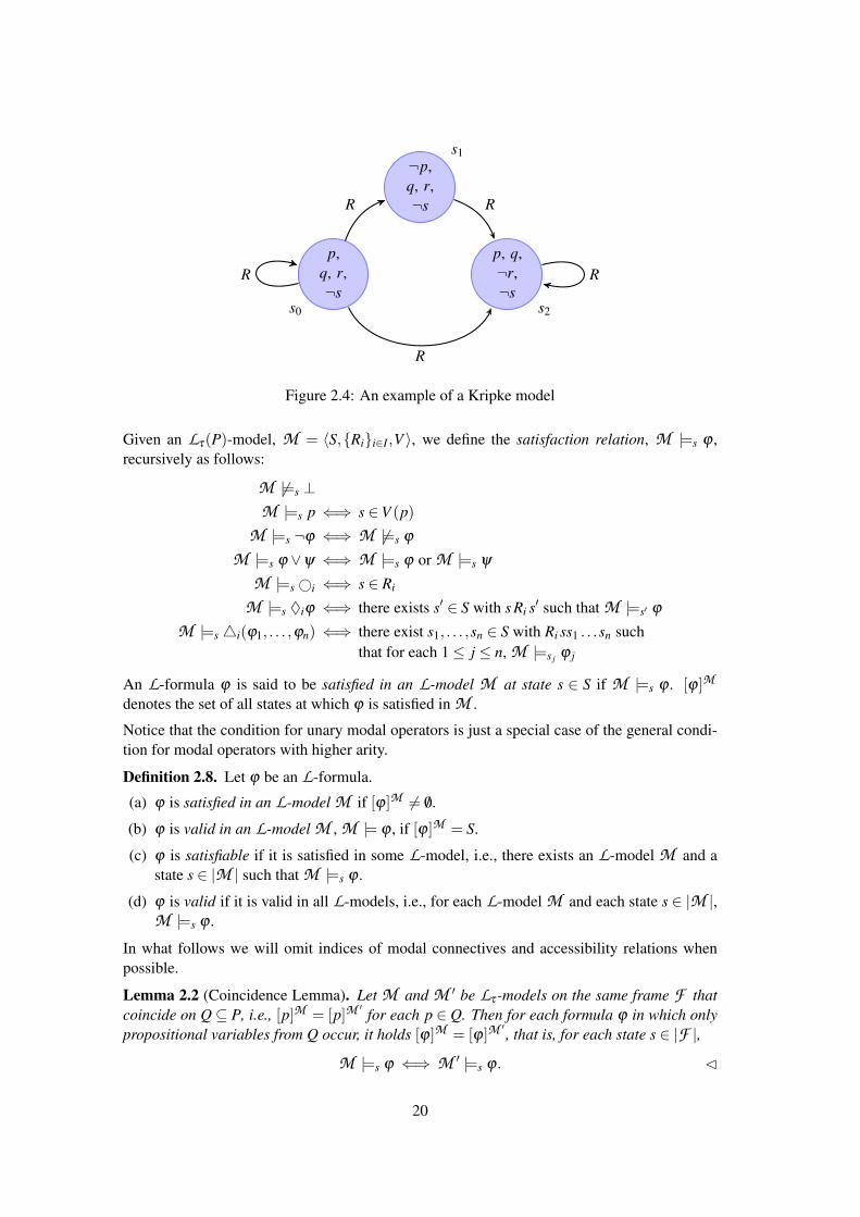
If P is understood, we will refer to Lτ(P)-models as τ-models. In the situation of basic modallanguages τ-models are also called Kripke models. Kripke models can be depicted as directedmulti-graphs that have both a vertex and an edge labeling (see Figure 2.4): vertices are labeledby a truth assignment and edges by accessibility relations.

19

p,q, r,¬s

s0

¬p,q, r,¬s

s1

p, q,¬r,¬s

s2

R

R

R

R

R

Figure 2.4: An example of a Kripke model

Given an Lτ(P)-model, M = 〈S,{Ri}i∈I,V 〉, we define the satisfaction relation, M |=s ϕ ,recursively as follows:

M 6|=s ⊥M |=s p ⇐⇒ s ∈V (p)

M |=s ¬ϕ ⇐⇒ M 6|=s ϕ

M |=s ϕ ∨ψ ⇐⇒ M |=s ϕ or M |=s ψ

M |=s ©i ⇐⇒ s ∈ Ri

M |=s ♦iϕ ⇐⇒ there exists s′ ∈ S with s Ri s′ such that M |=s′ ϕ

M |=s 4i(ϕ1, . . . ,ϕn) ⇐⇒ there exist s1, . . . ,sn ∈ S with Ri ss1 . . .sn suchthat for each 1≤ j ≤ n, M |=s j ϕ j

An L-formula ϕ is said to be satisfied in an L-model M at state s ∈ S if M |=s ϕ . [ϕ]M

denotes the set of all states at which ϕ is satisfied in M .

Notice that the condition for unary modal operators is just a special case of the general condi-tion for modal operators with higher arity.

Definition 2.8. Let ϕ be an L-formula.

(a) ϕ is satisfied in an L-model M if [ϕ]M 6= /0.

(b) ϕ is valid in an L-model M , M |= ϕ , if [ϕ]M = S.

(c) ϕ is satisfiable if it is satisfied in some L-model, i.e., there exists an L-model M and astate s ∈ |M | such that M |=s ϕ .

(d) ϕ is valid if it is valid in all L-models, i.e., for each L-model M and each state s ∈ |M |,M |=s ϕ .

In what follows we will omit indices of modal connectives and accessibility relations whenpossible.

Lemma 2.2 (Coincidence Lemma). Let M and M ′ be Lτ -models on the same frame F thatcoincide on Q⊆ P, i.e., [p]M = [p]M

′for each p ∈ Q. Then for each formula ϕ in which only

propositional variables from Q occur, it holds [ϕ]M = [ϕ]M′, that is, for each state s ∈ |F |,

M |=s ϕ ⇐⇒ M ′ |=s ϕ. C

20

Lemma 2.3 (Substitution Lemma). Let σ : P→ Lτ(P) be a substitution and M = 〈F ,V 〉 bean L-model. Let M σ denote the model 〈F ,V σ 〉 where V σ is defined by V σ (p) := {s ∈ |F | :M |=s σ(p)}. Then for all formulae ϕ and all states s ∈ |F |,

M σ |=s ϕ ⇐⇒ M |=s ϕσ . C

Lemma 2.4. The following formulae are valid in all L-models:

(a) ♦(ϕ ∨ψ)↔ (♦ϕ ∨♦ψ)

(b) �(ϕ ∧ψ)↔ (�ϕ ∧�ψ)

(c) ♦(ϕ ∧ψ)→ (♦ϕ ∧♦ψ)

(d) (�ϕ ∨�ψ)→�(ϕ ∨ψ)

(e) �>

(f) �(ϕ→ψ)→ (�ϕ→�ψ)

(g) �(ϕ→ψ)→ (♦ϕ→♦ψ)

(h) (♦p∧�q)→♦(p∧q)

Furthermore, it holds:

(i) If ϕ is valid in M , then so is �ϕ .

(j) If ϕ is valid and σ : P→ Lτ(P) is a substitution, then ϕσ is valid. C

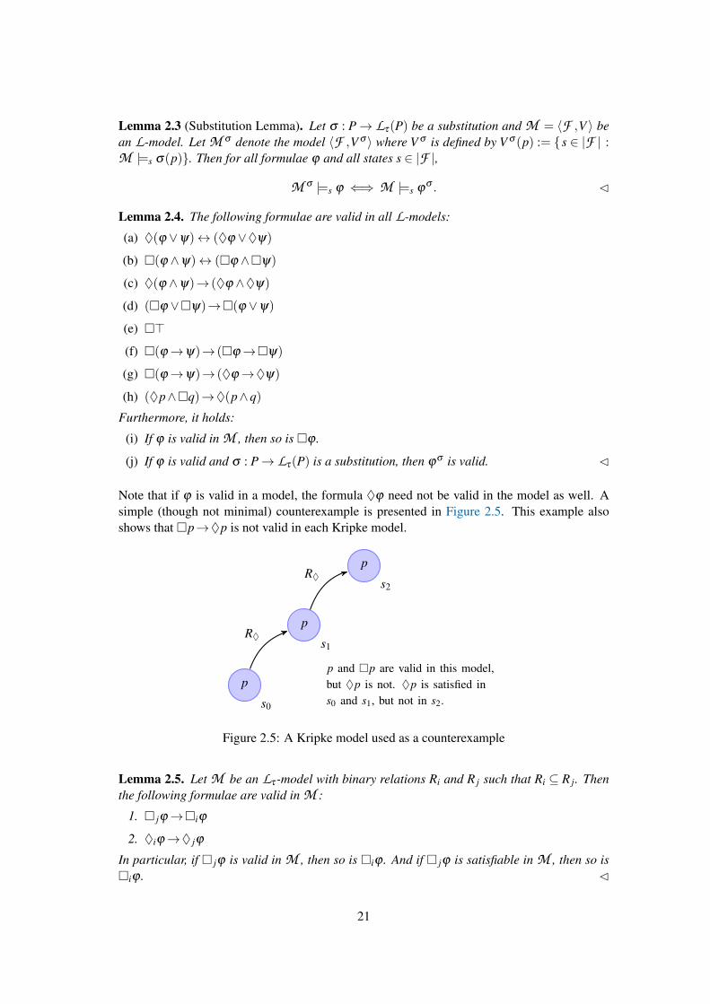
Note that if ϕ is valid in a model, the formula ♦ϕ need not be valid in the model as well. Asimple (though not minimal) counterexample is presented in Figure 2.5. This example alsoshows that �p→♦p is not valid in each Kripke model.

p

s0

p

s1

p

s2

R♦

R♦

p and �p are valid in this model,but ♦p is not. ♦p is satisfied ins0 and s1, but not in s2.

Figure 2.5: A Kripke model used as a counterexample

Lemma 2.5. Let M be an Lτ -model with binary relations Ri and R j such that Ri ⊆ R j. Thenthe following formulae are valid in M :

1. � jϕ→�iϕ

2. ♦iϕ→♦ jϕ

In particular, if � jϕ is valid in M , then so is �iϕ . And if � jϕ is satisfiable in M , then so is�iϕ . C

21

In what follows we will consider in more detail the satisfaction condition for some of the specialmodal logics presented in the previous section.

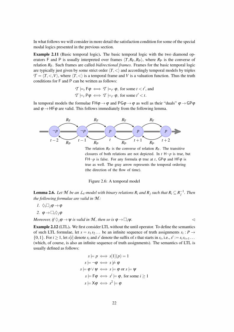
Example 2.11 (Basic temporal logic). The basic temporal logic with the two diamond op-erators F and P is usually interpreted over frames 〈T,RF,RP〉, where RP is the converse ofrelation RF. Such frames are called bidirectional frames. Frames for the basic temporal logicare typically just given by some strict order 〈T,<〉 and accordingly temporal models by triplesT = 〈T,<,V 〉, where 〈T,<〉 is a temporal frame and V is a valuation function. Thus the truthconditions for F and P can be written as follows:

T |=t Fϕ ⇐⇒ T |=t ′ ϕ, for some t < t ′, and

T |=t Pϕ ⇐⇒ T |=t ′ ϕ, for some t ′ < t.

In temporal models the formulae FHϕ→ϕ and PGϕ→ϕ as well as their “duals” ϕ→GPϕ

and ϕ→HFϕ are valid. This follows immediately from the following lemma.

p

t

p

t +1

p

t +2

¬p

t−1

¬p

t−2

RF RF RF RF

RPRPRPRP

The relation RP is the converse of relation RF. The transitiveclosures of both relations are not depicted. In t H¬p is true, butFH¬p is false. For any formula ϕ true at t, GPϕ and HFϕ istrue as well. The gray arrow represents the temporal ordering(the direction of the flow of time).

Figure 2.6: A temporal model

Lemma 2.6. Let M be an Lτ -model with binary relations Ri and R j such that Ri ⊆ R−1j . Then

the following formulae are valid in M :

1. ♦i� jϕ→ϕ

2. ϕ→�i♦ jϕ

Moreover, if ♦ jϕ→ψ is valid in M , then so is ϕ→�iψ . C

Example 2.12 (LTL). We first consider LTL without the until operator. To define the semanticsof such LTL formulae, let s = s1 s2 . . . be an infinite sequence of truth assignments si : P→{0,1}. For i≥ 1, let s[i] denote si and si denote the suffix of s that starts in si, i.e., si := si si+1 . . .(which, of course, is also an infinite sequence of truth assignments). The semantics of LTL isusually defined as follows:

s |= p ⇐⇒ s[1](p) = 1

s |= ¬ϕ ⇐⇒ s 6|= ϕ

s |= ϕ ∨ψ ⇐⇒ s |= ϕ or s |= ψ

s |= Fϕ ⇐⇒ si |= ϕ, for some i≥ 1

s |= Xϕ ⇐⇒ s2 |= ϕ

22

It is clear that this semantics can also be cast in terms of Kripke models as introduced in thissection. To see this, define such a model M s as follows:

S :=N

RF := Succ∗

RX := Succ

V (s) := { i ∈N : s[i](p) = 1}

where Succ := {(i, i+ 1) : i ∈ N} denotes the successor relation on N. Then for each LTLformula ϕ and each i ∈N, it holds:

M s |=i ϕ ⇐⇒ si |= ϕ.

In LTL with “until” the truth condition for U is given by

s |= U(ϕ,ψ) ⇐⇒ there exist i ≥ 1 such that si |= ψ and s j |= ϕ

for each 1≤ j < i

which corresponds to the following truth condition for temporal models:

M |=t U(ϕ,ψ) ⇐⇒ there is a t ′ ≥ t with M |=t ′ ψ and M |=t ′′ ϕ

for each t ≤ t ′′ < t ′.

Example 2.13 (Regular PDL). PDL- and in particular regular PDL-formulae are also inter-preted on Kripke models, but (as in the case of temporal logic) the class of considered PDL-models is restricted to Kripke-models satisfying the following equations:

Rπ1∪π2 = Rπ1 ∪Rπ2

Rπ1;π2 = Rπ1 ◦Rπ2

Rπ∗ = (Rπ)∗

that is, the accessibility relations need to satisfy dependency conditions to express the intendedmeaning of the constructors of programs.

Example 2.14 (ALC ). As mentioned in Example 2.9, in the description logic ALC complexconcepts are generated from concept names and role names by applying concept negation (¬C),concept intersection (C1uC2), concept disjunction (C1tC2), universal restrictions (∀r.C), andexistential restrictions (∃r.C). As simple ALC -formulae we confine here to simple assertionsof the form a : C or (a1,a2) : R. To interpret this formal language one considers relationalstructures of the form

M =⟨U,rM

1 , . . . ,rMn ,CM

1 , . . . ,CMm ,aM

1 , . . . ,aMk⟩

where U is a non-empty set (universe). For each role name ri, rMi is a binary relation on U , for

each concept name C j, CMj is a subset of U , and for each individual name al , aM

l is an element

23

of U . Inductively, we define the interpretation of concept terms as follows:

>M :=U

⊥M := /0

(¬C)M :=U \CM

(CuC′)M :=CM ∩C′M

(CtC′)M :=CM ∪C′M

(∃r.C)M := {x ∈U : there is a y ∈CM with x rM y}

(∀r.C)M := {x ∈U : for each y ∈U with x rM y, y ∈CM }

Then the satisfaction concept for simple ALC -formulae is defined by:

M |= a : C ⇐⇒ aM ∈CM

M |= (a1,a2) : R ⇐⇒ aM RM bM

An ALC -formula ϕ is said to be satisfiable if there exists an ALC -model M with M |= ϕ .

Example 2.15 (Arrow logic). Remember that the modal type of arrow logic, τ→ consists of abinary operator ◦, a unary one⊗, and a nullary one 1′. Then an arrow model is given by a tupleM = 〈A,C,R, I,V 〉, where 〈A,C,R, I〉 is an arrow frame (see Example 2.10). The satisfactionrelation then is exactly the satisfaction relation defined for τ→-models, i.e.,

M |=a 1′ ⇐⇒ I a

M |=a ⊗ϕ ⇐⇒ M |=b ϕ , for some b ∈ A with a R b

M |=a ϕ ◦ψ ⇐⇒ M |=b ϕ and M |=c ψ , for some b,c ∈ A with C abc

2.4 Constructing models

In this section we will introduce some basic methods on how models can be constructed fromother methods.

Definition 2.9. Let M = 〈S,{Ri}i∈I,V 〉 and M ′ = 〈S′,{R′i}i∈I,V ′〉 be L-models. A functionf : S→ S′ is called a bounded morphism if the following conditions are satisfied:

(a) f is a homomorphism of the frames (conceived of as relational structures).

(b) For all s ∈ S,s′1, . . . ,s′n ∈ S′, if R′i f (s)s′1 . . .s

′n, then there exist s1, . . . ,sn ∈ S with f (si) = s′i

such that Ri ss1 . . .sn. (If Ri is unary, this condition should be read as: if f (s) ∈ R′i, thens ∈ Ri.)

(c) For each s ∈ S and each p ∈ P, s ∈V (p) if and only if f (s) ∈V ′(p).

Condition (a) is called the forth condition and (b) the back condition. In the case of basic modallanguages these two conditions can be restated by:

s1 Ri s2⇒ f (s1)R′i f (s2)

f (s1)R′i s′2⇒ s1 Ri s and f (s) = s′2 for some s ∈ S.

Similarly, the concept of bounded morphism between frames, f : F → F ′, is introduced (i.e.f : S→ S′ is a function satisfying the forth and back conditions of Definition 2.9).

24

Proposition 2.7 (Invariance under bounded morphisms). Let f : M →M ′ be a bounded mor-phism of L-models. Then for each s ∈ S and each L-formula ϕ ,

M |=s ϕ ⇐⇒ M ′ |= f (s) ϕ.

Proof. The proof proceeds by induction on the length of formulae. Indeed, for propositionalvariables the claim follows immediately from Definition 2.9(c). And if ϕ is the formula ⊥,nothing is to be shown.

Assume now that ϕ is a formula of length n and that the claim holds for all formulae of length< n. If ϕ has the form ¬ϕ ′, it holds

M |=s ¬ϕ′ ⇐⇒ M 6|=s ϕ

′

⇐⇒ M ′ 6|= f (s) ϕ′

⇐⇒ M ′ |= f (s) ¬ϕ′.

In case ϕ has the form ϕ1∨ϕ2, we obtain

M |=s ϕ1∨ϕ2 ⇐⇒ M |=s ϕ1 or M |=s ϕ2

⇐⇒ M ′ |= f (s) ϕ1 or M ′ |= f (s) ϕ2

⇐⇒ M ′ |= f (s) ϕ1∨ϕ2.

If ϕ has the form ©i,

M |=s ©i ⇐⇒ s ∈ Ri ⇐⇒ f (s) ∈ R′i ⇐⇒ M ′ |= f (s) ©i.

Finally if ϕ has the form4i(ϕ1, . . . ,ϕn), we obtain:

M |=s 4i(ϕ1, . . . ,ϕn) ⇐⇒ there are s1, . . . ,sn ∈ S with Ri ss1 . . .sn andM |=si ϕi for each 1≤ i≤ n

⇐⇒ there are s1, . . . ,sn ∈ S with R′i f (s) f (s1) . . . f (sn) andM ′ |= f (si) ϕi for each 1≤ i≤ n

⇐⇒ there are s′1, . . . ,s′n ∈ S′ with R′i f (s)s′1 . . .s

′n and

M ′ |=s′i ϕi for each 1≤ i≤ n

⇐⇒ M ′ |= f (s) 4i(ϕ1, . . . ,ϕn).

Here in one direction the forth condition and in the other direction the back condition ofbounded morphisms is used. In all cases the induction hypothesis has been applied to formulaeof shorter length. C

Corollary 2.8. Let f : F → F ′ be a bounded morphism of τ-frames that is surjective. Thenfor each formula ϕ , if ϕ is valid in each model defined on frame F , then ϕ is valid in eachmodel defined on frame F ′.

Proof. We prove the contraposition of the claim: Assume that there is a model M ′ = 〈F ′,V ′〉and a state s′ of F ′ such that M ′ 6|=s′ ϕ . Define a model M on F by V (p) := {s ∈ S :M ′ |= f (s) p}. Then f is a bounded morphism of the L-models. Since f is surjective, thereexists an s ∈ S with f (s) = s′. By Proposition 2.7, it follows that M 6|=s ϕ . This shows that ϕ

is not valid in each model over F . C

25

Definition 2.10 (Submodel). Let M = 〈S,{Ri}i∈I,V 〉 be an L-model and S′ be a non-emptysubset of S. The L-model M ′ = 〈S′,{R′i}i∈I,V ′〉 defined by

R′i := Ri∩Sri and V ′(p) :=V (p)∩S′

(where for each i ∈ I, ri is the arity of Ri and p ∈ P) is called the submodel of M induced by S′.Given S′, let <S′> denote the smallest superset of S′ that is closed with respect to all relationsRi in M , in the following sense: for i ∈ I and s,s1, . . . ,sn ∈ S it holds:

s ∈<S′>, Ri ss1 . . .sn⇒ s1, . . . ,sn ∈<S′>.

Then the submodel of M generated by S′ is the submodel of M that is induced by <S′>. Agenerated submodel of M is any submodel that is generated by some subset of S. A point-generated submodel is a submodel that is generated by a singleton set. When a model ispoint-generated by {s0}, we also say that the model is rooted, and refer to s0 as its root.

Proposition 2.9. Let M = 〈S,{Ri}i∈I,V 〉 be an L-model, S′ be a non-empty subset of S, andM ′ be the submodel of M generated by S′. Then the inclusion function ι : <S′> ↪→ S is abounded morphism. In particular, for each s ∈<S′> and each L-formula ϕ ,

M ′ |=s ϕ ⇐⇒ M |=s ϕ.

Proof. It can easily be shown that ι : <S′> ↪→ S is a bounded morphism of L-models. Thesecond claim then follows immediately from Proposition 2.7. C

Definition 2.11 (Disjoint union). Let {M j} j∈J be a family of pairwise disjoint L-modelsM j = 〈S j,{R j

i }i∈I,V j〉, i.e., S j ∩ S j′ = /0 for all j, j′ ∈ J with j 6= j′. Then define an L-model⊎j∈J M j = 〈S,{Ri}i∈I,V 〉 by

S :=⋃j∈J

S j, Ri :=⋃j∈J

R ji , and V (p) :=

⋃j∈J

V j(p)

(for i ∈ I and p ∈ P). This model is called the disjoint union of the models M j.

Proposition 2.10. Let {M j} j∈J be a family of pairwise disjoint L-models. Then for eachj ∈ J, M j is a generated submodel of

⊎j∈J M j and the inclusion function ι : M j ↪→

⊎j∈J M j is

a bounded morphism. That is, for each s ∈ S j and each L-formula ϕ ,

M j |=s ϕ ⇐⇒⊎j∈J

M j |=s ϕ.

Proof. In fact, each M j is a submodel (generated by S j) of⊎

j∈J M j. Thus the claim followsfrom Proposition 2.9. C

Example 2.16. Consider the unary modal operator A, semantically defined by: M |=s Aϕ ifand only if for each state s′ ∈M , M |=s′ ϕ . Is there a definition of Aϕ in the basic modallanguage (in a way similar as we defined the � operator in terms of ♦)?Assume that there exists such a definition, i.e., a formula schema α(ϕ) in the basic modallanguage such that for each model M and each state s, M |=s α(ϕ) if and only if M |=s Aϕ .For a fixed propositional variable p, it then holds,

M |=s α(p) ⇐⇒ M |=s Aϕ. (∗)

26

Consider now two disjoint models M1 and M2 such that p is true in M1 in every state, butfalse in M2 in some state s∗. Let s be a fixed state in M1. Then it follows M1 |=s Ap (bythe assumption on M1), and hence by (∗), M1 |=s α(p). Because α(p) is a formula in thebasic modal language, it follows by Proposition 2.10, M1 ]M2 |=s α(p) and hence by (∗),M1]M2 |=s∗ p. By Proposition 2.10, we obtain M2 |=s∗ p — in contradiction to the choice ofs∗ in M2.

2.5 Translating modal logic into first-order logic

Modal logic is an extension of propositional logic, syntactically as well as semantically. Buthow does modal logic compare to first order logic? From the modal-logical semantics definedpreviously it is obvious that modal logic can be embedded into first order logic (FOL). Moreprecisely, there is a standard translation of modal logic (with the standard relational semantics)into first-order logic (FOL). In this section we will spell out this translation in a precise wayand we will draw some immediate conclusions from theoretical results concerning FOL.In what follows, let L := Lτ(P) be a fixed language of modal logic. There is a first order lan-guage that is associated with Lτ(P) in a natural way, namely the language LFOL := LFOL(τ,P)with the following alphabet:

• denumerably many variables v0,v1,v2, . . . ;

• for each p ∈ P, a unary relation symbol Fp;

• for each4i ∈ τ , an ri +1-ary relation symbol Ai;

• logical symbols =, ¬,→, ∧, ∨, ∃, and ∀.That is, the signature of LFOL depends on the set of propositional variables and the similaritytype of Lτ(P).LFOL-formulae are defined in the usual manner (the set of LFOL-formulae is denoted by LFOLas well). In particular, this means that for each LFOL-formula ϕ and each variable x, ∀xϕ and∃xϕ are LFOL-formulae. One should recall usual notions of FOL such as free (occurrence ofa) variable, (variable) assignment, first order structure, etc: for example, a first-order LFOL-structure is a tuple

S =⟨

U,{ASi }i∈I,{FS

p }p∈P

⟩where each AS

i is an ri+1-ary relation on U and each FSp is a subset of U . A variable assignment

in S is simply a function a : V →U and the satisfaction relation is defined by:

S ,a |= Fp(x) ⇐⇒ a(x) ∈ FSp

S ,a |= Ai(x1, . . . ,xri+1) ⇐⇒ (a(x1), . . . ,a(xri+1)) ∈ ASi

S ,a |= x = y ⇐⇒ a(x) = a(y)

S ,a |= ¬ϕ ⇐⇒ S ,a 6|= ϕ

. . .

S ,a |= ∃xϕ ⇐⇒ S ,a[x 7→ u] |= ϕ for some u ∈U

S ,a |= ∀xϕ ⇐⇒ S ,a[x 7→ u] |= ϕ for each u ∈U

Here a[x 7→ u] is the variable assignment that coincides with a in the assignment of all variablesexcept x and assigns u to x. We write S |= ϕ if S ,a |= ϕ for each variable assignment a. ForLFOL-sentences (i.e., formulae in which no variable occurs free) the satisfaction relation does

27

not depend on the variable assignment, i.e., for each sentence ϕ , it holds S |= ϕ or S |= ¬ϕ .A set of LFOL-sentences is satisfiable if there exists an LFOL-structure S with S |= ϕ for eachϕ ∈ Σ. We write Φ(x) to denote a set of formulae in which at most variable x occurs free.Such a Φ(x) is called satisfiable if there exists a structure S and an element u ∈U such thatS ,(x 7→ u) |= ϕ for each ϕ ∈ Φ(x) (here (x 7→ u) refers to an arbitrary variable assignmenta with a(x) = u). Alternatively, we may expand LFOL by an individual constant c; then theset Φ(x)[x/c] resulting from replacing in each formula ϕ ∈ Φ(x) each free occurrence of x byc is a set of LFOL ∪{c}-sentences. It is easy to see that Φ(x)[x/c] is satisfiable (as a set ofLFOL∪{c}-sentences) if and only if Φ(x) is satisfiable (as a set of LFOL-formulae).

We now define the standard translation of Lτ(P) into LFOL(τ,P), which is a mapping

STx : Lτ(P)→ LFOL(τ,P)

where x is some variable of LFOL. Then define

STx(p) = Fp(x)

STx(⊥) = x 6= x

STx(¬ϕ) = ¬STx(ϕ)

STx((ϕ ∨ψ)) = (STx(ϕ)∨STx(ψ))

STx(©i) = Ai(x)

STx(♦iϕ) = ∃y(Ai(x,y)∧STy(ϕ))

STx(4i(ϕ1, . . . ,ϕri)) = ∃y1 . . .yri(Ai(x,y1, . . . ,yri)∧∧

1≤ j≤ri

STyi(ϕi))

where y and y1, . . . ,yri are the variables with smallest index (in the sequence v0,v1, . . . ) thatdo not occur in STx(ϕ) and all the STx(ϕi), respectively. Notice that in STx(ϕ) exactly onevariable occurs free (not within the scope of a quantifier), namely the variable x.

Example 2.17. As an example consider the formula ♦♦ϕ→♦ϕ . The standard translation ofthis formula is

STx(¬♦♦p∨♦p) = ¬∃y(A(x,y)∧∃z(A(y,z)∧Fp(z)))∨∃y(A(x,y)∧Fp(y))),

where y,z are suitable variables of LFOL. This formula is FO-equivalent to:

∃y(A(x,y)∧∃z(A(y,z)∧Fp(z)))→∃y(A(x,y)∧Fp(y))),

and this formula in turn is equivalent to:

∃yz(A(x,y)∧A(y,z)∧Fp(z))→∃y(A(x,y)∧Fp(y)).

By contraposition, we obtain:

∀y(A(x,y)→¬Fp(y))→∀yz(A(x,y)∧A(y,z)→¬Fp(z)).

In section 3 we will see that the formula ♦♦ϕ→♦ϕ is closely related to the transitivity of theaccessibility relation. This connection becomes more obvious if we consider a fixed interpre-tation of the predicates Fp(v): let us assume that for each variable v,

Fp(v)⇐⇒¬A(x,v)

(note that x is a fixed variable). Thus, the formula on the right-hand side of the equation isequivalent to

∀yz(A(x,y)∧A(y,z)→A(x,z)).

28

This observation is the starting point of the so-called correspondence theory of modal logic.Correspondence theory deals with the question of which formulae of modal logic correspond tofirst order properties of Kripke frames. We will discuss this in more detail in the next section.

How are models of Lτ and models of LFOL related to each other? Let M = 〈S,{Ri}i,V 〉 be anL-model (i.e., a Kripke model in the case of basic modal languages). Then the ordered pairSM = 〈S,{ASM

i }i,{FSMp }p〉 with

FSMp :=V (p) and ASM

i := Ri

is an LFOL-structure. Conversely, if S = 〈U,{ASi }i,{FS

p }p}〉 is an LFOL(τ,P)-structure, thenthe triple M S = 〈U,{Ri}i,V 〉 with

Ri := ASi and V (p) := FS

p

defines an Lτ(P)-model.

Theorem 2.11 (Standard translation into FOL). The mapping M 7→ SM defines a bijectionbetween the class of Lτ(P)-models and the class of first order LFOL(τ,P)-structures. Moreover,for each Lτ(P)-formula ϕ , it holds:

(a) M |=s ϕ if and only if SM ,(x 7→ s) |= STx(ϕ);

(b) M |= ϕ if and only if SM |= ∀x STx(ϕ).

Proof. Obviously, (b) follows from (a). And (a) can easily be proven by induction on ϕ . C

2.6 Consequence relation and compactness

In propositional logic, the (semantic) consequence relation, Σ |= ϕ , is defined as follows: ϕ

follows from Σ if each truth assignment that makes all formulae in Σ true, makes ϕ true as well.In modal logic there are at least two alternative definitions of consequence, since there aredifferent concepts of a formula being true in a model. In the global reading, Σ |= ϕ means thatfor each model in which each formula of Σ is valid, ϕ is valid as well. In the local reading,Σ |= ϕ means that for each model and each state s in that model in which each formula of Σ issatisfied, ϕ is satisfied as well. In what follows we use the local definition.

Definition 2.12 (Semantic consequence). The formula ϕ is a consequence of a set of formulae,Σ, Σ |= ϕ , if in each state s of each model M , M |=s Σ implies M |=s ϕ .

Lemma 2.12. (a) /0 |= ϕ if and only if ϕ is valid.

(b) Σ 6|= ϕ if and only if Σ∪{¬ϕ} is satisfiable. C

FOL is characterized by two properties. First, FOL is compact, i.e., a set of first order sen-tences (formulae without free variables) is satisfiable if and only if each of its finite subsets issatisfiable. Secondly, FOL has the Lowenheim-Skolem property, i.e., each set of first order sen-tences (in a language with countable signature) that is satisfiable in some model is satisfiablein a model that is defined on a countable domain (here and in what follows, “countable” means“finite” or “countably infinite”). In fact, as was proven by Lindstroem, FOL is the strongestlogic that is compact and satisfies Lowenheim-Skolem (see Ebbinghaus et al., 2007, chapterXIII).In the sequel we will show that analogous results carry over to modal logic. Thereby we willapply the standard translation introduced above.

29

Theorem 2.13 (Compactness for models). Let Σ be a set of Lτ(P)-formulae. If each finitesubset of Σ is satisfiable, then so is Σ.

Proof. Assume that each finite subset of Σ is satisfiable in some L-model. We expand LFOL bya new individual constant c and consider the set of LFOL∪{c}-formulae

STx/c(Σ) := {(STx(ϕ))[x/c] : ϕ ∈ Σ}.

First we show that each finite subset of STx/c(Σ) is satisfiable (in some first-order structure).For proof by contradiction assume that there is a finite subset {ϕ1, . . . ,ϕn} of Σ such that

{(STx(ϕ1))[x/c], . . . ,(STx(ϕn))[x/c]}

is not satisfiable. This means that

n∧i=1

(STx(ϕi))[x/c] = (n∧

i=1

STx(ϕi))[x/c] = (STx(n∧

i=1

ϕi))[x/c]

is not satisfiable either. But each finite subset of Σ is satisfiable, in particular {ϕ1, . . . ,ϕn}.Hence there is a (modal-logical) L-model M with some state s∗ such that M |=s∗

∧ni=1 ϕi. By

Theorem 2.11 we obtain that SM ,(x 7→ s∗) |= STx(∧n

i=1 ϕi). SM can be expanded to an LFOL∪{c}-model S ′ if we set cS ′ := s∗. Obviously S ′ |= (STx(

∧ni=1 ϕi))[x/c]— in contradiction to

our observation that this set is not satisfiable.Thus, each finite subset of STx/c(Σ) is satisfiable. By compactness of FOL, STx/c(Σ) must besatisfiable as well. That is, there exists an LFOL∪{c}-structure S ′ with S ′ |= (STx(ϕ))[x/c] foreach ϕ ∈ Σ. If we “forget” in S ′ the interpretation of c, we obtain an LFOL-structure S with

S ,(x 7→ cS ′) |= STx(ϕ)

for each ϕ ∈ Σ. By Theorem 2.11, it follows

M S |=cS ′ ϕ

for each ϕ ∈ Σ. Thus Σ is satisfiable in M S . C

The compactness theorem stated above can just serve as some initial observation. Usually, oneis interested in compactness results that relate the model of the large set Σ somehow to themodels of its finite subsets. We come back to this point later.

Theorem 2.14 (Lowenheim-Skolem). Let L be a basic modal language with countably manypropositional variables and Σ be a set of L-formulae. If Σ is satisfiable in some L-model, thenΣ is satisfiable in a countable L-model M (i.e., M is defined on a finite or countably infiniteset of states).

Proof. Assume that Σ is satisfiable. That is, there exists an L-model M with a state s such thatM |=s Σ. By Theorem 2.11, we obtain that

SM ,(x 7→ s) |= STx(Σ),

i.e., the set of sentences STx/c(Σ) is satisfiable in an LFOL ∪{c}-structure (again c is a newindividual constant). Since FOL has the Lowenheim-Skolem property, STx/c(Σ) is satisfiable

30

in a countable LFOL∪{c}-structure S ′, i.e., if we drop c from the signature, S ′ can be reducedto an LFOL-structure S with

S ,(x 7→ cS ′) |= STx(Σ),

By Theorem 2.11, S defines an Lτ -model M S such that

M S |=cS ′ Σ,

which is obviously countable. Thus, Σ is satisfiable in a countable L-model. C

2.7 Expressiveness

What is the expressive power of modal logic? What can be expressed by modal formulae?The key idea to investigate such questions is that expressiveness of a formal language can bemeasured by its power of making distinctions between different “situations”. Adapted to ourcontext, we can put it more precisely as follows: Consider Kripke models M and M ′ andstates s and s′ of M and M ′, respectively. Is there any modal formula by which s and s′ can bedistinguished?

Definition 2.13. The type of s in M is defined as the set

TM (s) := {ϕ : M |=s ϕ}.

States s and s′ are said to be modally equivalent, s≡M ,M ′ s′, if TM (s) = TM ′(s′).

As has been proven in section 2.4, a sufficient criterion for modal equivalence is the existenceof a bounded morphism, i.e., if f is a bounded morphism from M to M ′, then for each state sof M ,

s≡M ,M ′ f (s).

However, the converse of this observation does not hold in general.A somewhat weaker notion than that of a bounded morphism is that of bisimulation. We willsee that modal equivalence follows from bisimilarity and that there is a fairly wide class ofmodels where the converse of this implication holds, too. For the sake of simplicity we confineto basic modal languages with one modality.

Definition 2.14. Let M = 〈S,R,V 〉 and M ′ = 〈S′,R′,V ′〉 be Kripke models for L♦(P). Anon-void relation Z ⊆ S× S′ is said to be a bisimulation between M and M ′ if the followingconditions are satisfied:

(a) For all s,s′ with s Z s′ and each p ∈ P, s ∈V (p) if and only if s′ ∈V ′(p);

(b) If s Z s′ and s Rt, then there exists a t ′ ∈ S′ with t Z t ′ and s′ R′ t ′ (forth condition);

(c) If s Z s′ and s′R′t ′, then there exists a t ∈ S with t Z t ′ and s Rt (back condition).

States s and s′ are called bisimilar, s!M ,M ′ s′, if there exists a bisimulation Z between Mand M ′ with s Z s′.

Obviously, the notion of bisimulation provides a generalization of the notion of p-morphism: p-morphisms are exactly those bisimulations that are left-total and functional. Before illustratingthis new concept by examples, we mention a fundamental statement.

31

Proposition 2.15. Let M = 〈S,R,V 〉 and M ′ = 〈S′,R′,V ′〉 be Kripke models. Let s ∈ S ands′ ∈ S′ be states such that s!M ,M ′ s′. Then s and s′ are modally equivalent, i.e., for eachformula ϕ ,

M |=s ϕ ⇐⇒ M ′ |=s′ ϕ.

Proof. Straight forward, see the proof of Proposition 2.7. C

In the situation depicted in Figure 2.7, the states s and s′ are bisimilar if we assume that inall nodes all propositional variables are true. The bisimulation presented there is a bounded

s

R R

R

s′

R′

R′

R′

Figure 2.7: Example of a bisimulation

morphism, obviously. But in general, not each bisimulation defines such a morphism. In thesituation of Figure 2.8, for example, we can construct step by step a bisimulation from theinitial link between states s and s′. However, it can be shown that there does not exist anybounded morphism f from the model on the left-hand side to that on the right-hand side withf (s) = s′.

s

R

R R

s′

R′

R′

R′

R′

Figure 2.8: Is there a bisimulation with s Z s′?

A more interesting, but also more technical example is given by a new kind of model construc-tion, namely by the method of “unraveling” a Kripke model. More precisely, it can be shownthat for each rooted Kripke model, there exists a tree-like Kripke model such that the roots ofthe models are bisimilar.To see this, let M = 〈S,R,V 〉 be a Kripke model with root s0 ∈ S. Define a tree-like model,M tree

s0= 〈S′,R′,V ′〉, by

S′ :={

s : s is a finite R-chain of length ns > 0 with s[1] = s0}

R′ :={(s, t) ∈ S′×S′ : s = (s0, . . . ,sn), t = (s0, . . . ,sn,sn+1)

}V ′(p) :=

{s ∈ S′ : s = (s0, . . . ,sn) ∈ S′ and sn ∈V (p)

}32

Then the relation

Z :={(

s, t)∈ S×S′ : t = (s0, . . . ,sn) and sn = s

}defines a bisimulation between M and M tree

s0. Moreover, the mapping

f : M trees0→M , (s0, . . . ,sn) 7→ sn

defines a surjective bounded morphism from M trees0

to M . Figure 2.9 depicts a simple example.

0

1

R

R

0

01 00

001 000

R′ R′

R′ R′

Figure 2.9: Unraveling a simple Kripke model

In general, the converse of Proposition 2.15 does not hold (see exercises). However, if werestrict consideration on image-finite models, then it is possible to establish that bisimilarityfollows from modal equivalence.

Definition 2.15. Let M = 〈S,R,V 〉 be a Kripke model. M is said to be image-finite if for eachs ∈ S,

sR := {s′ ∈ S : s R s′}

is finite.

Note that each finite model is image-finite.

Theorem 2.16 (Hennessy & Milner). Let M and M ′ be image-finite Kripke models. Then foreach state s of M and each state s′ of M ′,

s≡M ,M ′ s′ ⇐⇒ s!M ,M ′ s′.

Proof. The direction from right to left follows from Proposition 2.15. For the other directionwe show that the relation

Z :={(s,s′) ∈ S×S′ : s≡M ,M ′ s′

}defines a bisimulation between M and M ′. Condition (a) of Definition 2.14 is clear. Forcondition (b) let us suppose that s ≡M ,M ′ s′ and that s R t. Since M ′ is image-finite, we mayassume that

s′R′ = {s′0, . . . ,s′n}

33

with s′0, . . . ,s′n ∈ S′. Note that s′R′ is not empty: otherwise, M |=s′ �⊥, hence by s≡M ,M ′ s′,

M |=s �⊥ and thus, by s Rt, M |=t ⊥. Assume now for proof by contradiction that there doesnot exist any t ′ ∈ S′ with s′ R′ t ′ and t ≡M ,M ′ t ′, i.e., for each s′i ∈ s′R′, there is a formula ϕi

such thatM |=t ϕi and M ′ 6|=s′i ϕi.

Then it follows thatM |=s ♦(ϕ0∧·· ·∧ϕn),

and hence, by s≡M ,M ′ s′,M ′ |=s′ ♦(ϕ0∧·· ·∧ϕn).

Thus, there exists an s′i ∈ s′R′ with

M ′ |=s′i ϕ0∧·· ·∧ϕn

— in contradiction to M ′ 6|=s′i ϕi. The proof of condition (c) is similar to that of (b), using thefact that M is image-finite. C

How can the modal fragment can be characterized? Or, to put the question in other words:Which first order formulae are equivalent to the standard translation of some modal formula?

Definition 2.16. Let ϕ(x) be a LFOL(τ,P)-formula in which exactly one variable x occurs free.ϕ(x) is said to be invariant under bisimulation if for each pair of Kripke models M and M ′,each pair of possible state s and s′ of M and M ′, respectively, and each bisimulation Z betweenM and M ′ with s Z s′, it holds

MFOL,x 7→ s |= ϕ(x) ⇐⇒ M ′FOL,x 7→ s′ |= ϕ(x).

In terms of invariance under bisimulation the modal fragment can the ben characterized asfollows.

Theorem 2.17 (van Benthem). Let ϕ(x) be a LFOL-formula in which exactly one variable xoccurs free. Then the following statements are equivalent:

(a) ϕ(x) is equivalent to the standard translation STx(ψ) of some Lτ(P)-formula ψ .

(b) ϕ(x) is invariant under bisimulation. C

In this context it is worthwhile to discuss a game-theoretical characterization of bisimulations.Let M = 〈S,R,V 〉 and M = 〈S′,R′,V ′〉 be Kripke models, and let s0 and s′0 be states of M andM ′, respectively. The bisimulation game is then defined as follows:

• There are two players A (‘attacker’, ‘spoiler’) and D (‘defender’, ‘duplicator’). A seeks toshow that there does not exist any bisimulation Z between M and M ′ with s0 Z s′0, whileD tries to prevent this.

• The game is played in rounds (where the number of rounds, n, is fixed before the gameis started). There are two variants: the finite game and the infinite one (i.e., the game isplayed over infinitely many rounds).

34

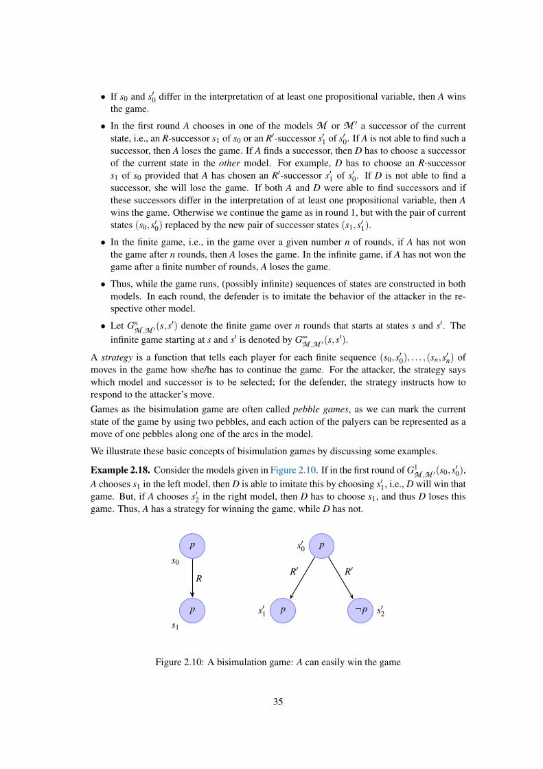
• If s0 and s′0 differ in the interpretation of at least one propositional variable, then A winsthe game.

• In the first round A chooses in one of the models M or M ′ a successor of the currentstate, i.e., an R-successor s1 of s0 or an R′-successor s′1 of s′0. If A is not able to find such asuccessor, then A loses the game. If A finds a successor, then D has to choose a successorof the current state in the other model. For example, D has to choose an R-successors1 of s0 provided that A has chosen an R′-successor s′1 of s′0. If D is not able to find asuccessor, she will lose the game. If both A and D were able to find successors and ifthese successors differ in the interpretation of at least one propositional variable, then Awins the game. Otherwise we continue the game as in round 1, but with the pair of currentstates (s0,s′0) replaced by the new pair of successor states (s1,s′1).

• In the finite game, i.e., in the game over a given number n of rounds, if A has not wonthe game after n rounds, then A loses the game. In the infinite game, if A has not won thegame after a finite number of rounds, A loses the game.

• Thus, while the game runs, (possibly infinite) sequences of states are constructed in bothmodels. In each round, the defender is to imitate the behavior of the attacker in the re-spective other model.

• Let GnM ,M ′(s,s′) denote the finite game over n rounds that starts at states s and s′. The

infinite game starting at s and s′ is denoted by G∞

M ,M ′(s,s′).

A strategy is a function that tells each player for each finite sequence (s0,s′0), . . . ,(sn,s′n) ofmoves in the game how she/he has to continue the game. For the attacker, the strategy sayswhich model and successor is to be selected; for the defender, the strategy instructs how torespond to the attacker’s move.Games as the bisimulation game are often called pebble games, as we can mark the currentstate of the game by using two pebbles, and each action of the palyers can be represented as amove of one pebbles along one of the arcs in the model.

We illustrate these basic concepts of bisimulation games by discussing some examples.

Example 2.18. Consider the models given in Figure 2.10. If in the first round of G1M ,M ′(s0,s′0),

A chooses s1 in the left model, then D is able to imitate this by choosing s′1, i.e., D will win thatgame. But, if A chooses s′2 in the right model, then D has to choose s1, and thus D loses thisgame. Thus, A has a strategy for winning the game, while D has not.

p

s0

p

s1

R

ps′0

ps′1 ¬p s′2

R′ R′

Figure 2.10: A bisimulation game: A can easily win the game

35

Example 2.19. Let us now consider the situation presented in Figure 2.11. Here A has variousstrategies for winning G2

M ,M ′(s0,s′0). For example, if A chooses in the model on the right sides′3, then D has to choose s1. Then A chooses s2 (note that A changes the model). Thus, D hasto choose s′4, but then she loses the game. Another strategy: In the first round, A chooses s1 inthe model on the left side. Then D has to choose between s′1 and s′3. But in each of both casesA can win the game by choosing s3 or s2, respectively.

ps0

ps1

p

s2

¬p

s3

R

R R

ps′0

p

s′1

p

s′2

p

s′3

¬p

s′4

R′

R′

R′

R′

Figure 2.11: Another example of a bisimulation game: A can win again

Without proof we now present the following theorems:

Theorem 2.18 (see Goranko and Otto (2007), Prop. 28). Let M = 〈S,R,V 〉 and M = 〈S′,R′,V ′〉be Kripke-models, let s be a state of M , and let s′ be state M ′. Then the following statementsare equivalent:

(a) D has a strategy for winning G∞

M ,M ′(s,s′).

(b) There exists a bisimulation Z between M and M ′ with s Z s′. C

The basic insight used in the proof of this theorem is that bisimulations can be interpreted aswinning strategy for the defender, and vice versa.

Theorem 2.19 (see Goranko and Otto (2007), Theorem 32). Let L♦(P) be a basic modal logicwith finitely many propositional variables. Let M = 〈S,R,V 〉 and M ′ = 〈S′,R′,V ′〉 be Kripkemodels and let s and s′ be states of M and M ′, respectively. Then the following statements areequivalent:

(a) D has a strategy for winning GnM ,M ′(s,s′).

(b) For all formulae ϕ of Lτ(P) with depthϕ ≤ n,

M |=s ϕ ⇐⇒ M ′ |=s′ ϕ C

36

Bibliographic remarks

A general reference for the material presented in this chapter is Blackburn et al. (2002), chap-ter 1 and chapter 2.Epistemic modal logics were presumably first discussed by von Wright (1951) and further de-veloped by Hintikka (1962). For an introduction to the philosophical foundations of epistemiclogics see, for example, Lenzen (1981) and for an introduction to epistemic logics and its com-putational aspects we refer to Fagin et al. (1995).Temporal logic (also known as tense logic) has been first studied by Prior (1957, 1967). Animportant field of application of temporal logic in computer science is the domain of modelchecking, i.e. the formal verification of system or software properties. The first logics studiedin this context are LTL (Linear-time Temporal Logic) and CTL (Computation Tree Logic) (see,e.g., Pnueli, 1977; Clarke et al., 1986; Emerson, 1990). A good starting point for further readingis the Stanford Encyclopedia of Philosophy on temporal logic (Galton, 2008).Propositional dynamic logic (PDL) is one of the logics discussed in the context of dynamiclogics, that is, logics for reasoning about computer programs: Pratt (1976) may count as astarting point in this research direction. PDL itself was introduced by Fischer and Ladner(1977).

37

38

3 Normal Modal Logics, Frame Classes, and Definability

In this section we introduce the concept of normal modal logics. We will discuss how classesof frames can be defined by axioms, how modal logics can be axiomatized, and a standardprocedure for proving soundness and completeness of such axiomatizations. Moreover, wewill learn more on special uni-modal logics.

3.1 Normal modal logics

In what follows we will confine to basic modal languages with a countable set of proposi-tional variables. Often we even confine to modal languages with a single modality. Almost allconcepts can be generalized to arbitrary modal languages in a straightforward way.

We start by introducing a rather general concept of modal logics.

Definition 3.1. A modal logic is a set of Lτ(P)-formulae, Λ, that contains all propositionaltautologies and is closed under modus ponens and (uniform) substitution, that is,

(a) If ϕ ∈ Λ and ϕ→ψ ∈ Λ, then ψ ∈ Λ.

(b) If ϕ ∈ Λ and σ : P→ Lτ(P) is a substitution, then ϕσ ∈ Λ.

A modal logic Λ is said to be normal if furthermore the following conditions are satisfied:

(c) Λ contains all valid Lτ(P)-formulae.

(d) Λ is closed under necessitation for each τ-modality ♦, i.e., if ϕ ∈ Λ, then �ϕ ∈ Λ.

Recall the small list of valid formulae presented in Lemma 2.4. All these formulae are con-tained in any normal modal logic, but not in every modal logic.

Remark 3.1. In the case of non-basic modal languages condition (d) in Definition 3.1 needsto be adapted. More precisely, (d) has to be replaced by

(d) If ϕ ∈ Λ, then5(⊥, . . . ,ϕ, . . . ,⊥) ∈ Λ.

Notice that no special requirements are imposed for 0-ary modalities.

Instead of conditions like “all propositional tautologies” or “all valid formulae”, one may re-sort to appropriate axiomatizations. For example, in order to guarantee that Λ contains allpropositional tautologies (see Definition 3.1), it suffices to require that all formulae of an ax-iomatization of propositional logic are included in Λ. In a similar way, for normal logics it issufficient that Λ contains all formulae of a suitable axiomatization of the set of formulae thatare valid in all models. As we will later see, for basic modal languages the following axiomssuffice (see also Lemma 2.4):

K �(p→q)→ (�p→�q)

Dual ♦p↔¬�¬p

Notice that in a setting in which the boxes � are chosen as primitives, axiom (Dual) is notneeded.

More generally, axiom K can be replaced by:

Ki5 5(. . . , p→q, . . .)→ (5(. . . , p, . . .)→5(. . . ,q, . . .))

39

It is easy to see that formulae of this form are valid in all models.

Some important examples of modal logics and normal modal logics are presented in the fol-lowing list.

Example 3.1. (a) The set of all Lτ -formulae is a normal modal logic, the inconsistent (nor-mal) modal logic.

(b) If {Λi}i∈I is a family of normal modal logics, then the intersection of all these logics⋂i Λi is a normal modal logic. In particular, for each pair of normal modal logics, Λ1 and

Λ2, Λ1∩Λ2 is a normal modal logic.

(c) Given a single frame F or a class of frames, C , the sets

Λ(F ) := {ϕ ∈ L : F |= ϕ}Λ(C ) := {ϕ ∈ L : F |= ϕ for each F in C}

are normal modal logics, the normal modal logics of F and C , respectively. Recall thatϕ is valid in a frame F , F |= ϕ , if it is valid in each model defined on that frame.

(d) Given a set of L-formulae Γ, there exists a smallest normal modal logic that contains Γ

as a subset. This logic is called the normal modal logic axiomatized by Γ and is denotedby Λ(Γ).

Remark 3.2. Are there “modal logics” that are not normal? Of course, the smallest modallogic is not a normal modal logic (since it does not contain axiom K or its variants). In fact, thesmallest modal logic is just propositional logic on top of a language with quasi-atoms (namelyformulae of the form ♦ϕ or4ϕ). But there are also more interesting non-normal modal logics,quasi-normal modal logics, regular modal logics, etc. Quasi-normal modal logics are modallogics that contain all theorems of K, but in which the application of the necessitation rule issomehow restricted (for example the Lewis systems S2 and S3 are quasi-normal). The mainsemantic difference is that in such systems validity of a formula is evaluated as truth in someselection of normal states. In regular modal logics the necessitation rule is replaced by theweaker rule: If ϕ→ψ ∈ Λ, then �ϕ→�ψ ∈ Λ.

Remark 3.3. We have introduced normal modal logics that are defined in terms of frames orframe classes and normal modal logics defined in terms of “axioms”. Both concepts shouldbe kept apart carefully. In what follows we will study the connection between these conceptsin more detail: for example, which normal modal logics (that is, a set of formulae) can beaxiomatized by a set of formulae (Λ = Λ(Γ) for some set of formulae Γ?) and which normalmodal logics are the normal logics defined by some (frame or) class of frames (Λ = Λ(C ) forsome frame class C ?).

For basic modal languages L with exactly one modality, the smallest normal modal logic iscalled K, for basic modal languages with m diamonds, the smallest normal modal logic iscalled K(m). In the general, polyadic case the smallest normal modal logic is called Kτ , whereτ is the modal similarity type of the considered modal language. All these logics are the normalmodal logics that are axiomatized by the empty set.Further normal modal logics can be generated on top of K if we consider the modal logicsaxiomatized by additional formulae. Prominent examples are the “axioms”:

T �p→ p (alternatively: p→♦p)

40

4 �p→��p (alternatively: ♦♦p→♦p)

E ♦p→�♦p (alternatively: ♦�p→�p)

B p→�♦p (alternatively: ♦�p→ p)

D �p→♦p

.3 ♦p∧♦q→♦(p∧♦q)∨♦(p∧q)∨♦(♦p∧q)

L �(�p→ p)→�p

Then, for example, the smallest normal modal logic that contains axiom T is called KT, thenormal modal logic axiomatized by {T,B} is called KTB, etc. Prominent examples are thelogics K4, KB, KBE, KD4, KDB, KL. Even more prominent logics have a special name suchas S4 (= KT4) or S5 (= KTE = KT4B). The latter example shows that, in general, the set ofaxioms used to generate the normal modal logic is not unique. Finally, some modal logics suchas S4 are the basis for new modal logics, for example, S4.1, S4.3, etc. Some of them will bestudied later in more detail.

Remark 3.4. In general, if Γ⊆ Γ′, then Λ(Γ)⊆Λ(Γ′). Thus, for some of the above mentionedmodal logics it is quite easy to see whether they are contained in another normal modal logic.More generally, it holds that if Γ ⊆ Λ(Γ′), then Λ(Γ) ⊆ Λ(Γ′). Hence it suffices to showthat all the axioms in Γ are contained in Λ(Γ′) (i.e., they are “derivable” from Γ′ using anaxiomatization of K and the “axioms” in Γ′).

Remark 3.5. Notice that adding axioms to system K may even result in the inconsistent logic.An example is the axiom set {T,L}, i.e., the modal logic KTL coincides with the inconsistentmodal logic.

3.2 Kripke frames and definability

What makes the relational semantics interesting is the close connection between valid “axioms”and formal properties of the accessibility relation in Kripke frames. In this section we willthrow a first glance on this connection. For the sake of simplicity, we will consider unimodallanguages. Then it is convenient to talk about reflexive, transitive, etc., Kripke frames, whenthe accessibility relation has the respective property.

Proposition 3.1. A Kripke frame F is reflexive if and only if axiom T is valid in F .

Proof. Assume first that F = 〈S,R〉 is a reflexive frame, and let M be an arbitrary Kripkemodel defined on F . For each s ∈ S, if M |=s p, then by reflexivity, there exists a state s′ ∈ Swith s R s′ and M |=s′ p, namely state s. Hence M |=s ♦p. This shows that T is satisfied ineach state in each model defined on F .For the other direction, assume that T is valid in F . We have to show that F is reflexive, i.e.,sRs for each s ∈ S. For an arbitrary s ∈ S define a model Ms on F with V (p) = {s}. Since T isvalid in F , it follows that Ms |=s p→♦p. Because of Ms |=s p, it follows Ms |=s ♦p. Hencethere exists an s′ ∈ S with s R s′ and Ms |=s′ p. Then it follows s = s′ and hence s R s. C

Proposition 3.2. A Kripke frame F is transitive if and only if axiom 4 is valid in F .

Proof. Assume first that F = 〈S,R〉 is a transitive frame, and let M be a Kripke model definedon F . For each s ∈ S, if M |=s ♦♦p, then there exist states s′,s′′ such that s R s′, s′ R s′′, and

41

M |=s′′ p. By transitivity of R, it follows s R s′′ and hence M |=s ♦p. This shows that 4 issatisfied in each state in each model defined on F .For the other direction, assume that 4 is valid in F . We have to show that F is transitive, i.e.,for all s,s′,s′′ ∈ S, s R s′ and s′ R s′′ implies s R s′′. For arbitrary such s,s′,s′′ define a modelM on F with V (p) = {s′′}. Then it holds M |=s′′ p, hence M |=s′ ♦p, and consequently,M |=s ♦♦p. Since 4 is valid in F and thus in M , it follows M |=s ♦p. Thus there exists astate s′′′ with s R s′′′ and M |=s′′′ p. Since p is true in s′′ only, it follows s′′ = s′′′ and hences R s′′— as to be shown. C

As indicated in Example 2.17, a different proof of the back direction could be as follows:consider s,s′,s′′ ∈ S, with s R s′ and s′ R s′′. Define a model M on F by V (p) := S\R[s]. Thenit follows M 6|=s ♦p (otherwise there would be an s′′′ ∈ S with s R s′′′ and M |=s′′′ p, and hences′′′ ∈ R[s] and s′′′ ∈ V (p)— in contradiction to the definition of V (p)). Since 4 is valid in M ,we obtain M 6|=s ♦♦p. Because of s R s′, we can conclude M 6|=s′ ♦p, and thus M 6|=s′′ p. Bydefinition of V (p), we obtain s′′ ∈ R[s], i.e., s R s′′— as to be shown.

Proposition 3.3. A Kripke frame F is Euclidean if and only if axiom E is valid in F .

Proof. Exercise. C

Proposition 3.4. A Kripke frame F is symmetric if and only if axiom B is valid in F .

Proof. Exercise. C

Proposition 3.5. A Kripke frame F is serial if and only if axiom D is valid in F .

Proof. Exercise. C

All these propositions claim that certain classes of frames are definable by formulae.

Definition 3.2. Let ϕ be an Lτ -formula, and let C and D be a classes of τ-frames.

(a) ϕ is said to define (or: characterize) C within D if for each τ-frame in D , F is in C ifand only if F |= ϕ .

(b) ϕ is said to define (or: characterize) C if ϕ defines C within the class of all τ-frames.

(c) In a similar way, we say that a set of Lτ -formulae ∆ defines (or characterizes) a class offrames (possibly within some other class of frames).

So what we have proven above is that T defines the class of reflexive frames, 4 the class oftransitive frames, B the class of symmetric frames, E the class of Euclidean frames, etc.

But what about the following axioms? Do similar “correspondence” results hold there as well?

Tc p→�p

Triv p↔�p

E1 �♦�p→ p

E2 ♦�p→�♦��p

Dc ♦p→�p

42

D1 �(�p→q)∨�(�q→ p)

F (�♦p∧�♦q)→♦(p∧q)

M �♦p→♦�p

G1 ♦�p→�♦p

BM p→�♦♦p

TM ♦�p→♦p

Lem0 �(p∧�p→q)∨�(q∧�q→ p)

H �(�p↔ p)→�p

Altn �p1∨�(p1→ p2)∨·· ·∨�(p1∧·· ·∧ pn→ pn+1)

N1 �(�(p→�p)→ p)→ (♦�p→ p)

H1 p→�(♦p→ p)

G0 ♦(p∧�q)→�(p∨♦q)

J1 �(�(p→�p)→ p)→ p

. . .

Candidate frame properties are the properties mentioned in Definition 2.1 and the following:

(a) The frame consists of a single reflexive state.

(b) The frame consists of single dead end.

(c) The frame consists of a single state.

(d) In the frame each state sees at most one state.

(e) In the frame each state sees at most n worlds.

(f) In the frame each state sees a dead end.

(g) The frame is convergent.

(h) The frame is universal.

(i) The frame is finite, reflexive, transitive, and symmetrical.

(j) The frame is finite, irreflexive, and transitive.

(k) . . .

Similar to the first-order language considered for the standard translation of a modal language,we can define the first-order frame language of a modal similarity type τ , LFOL(τ): just dropthe unary relation symbols introduced for the translation of propositional letters of Lτ(P). Thislanguage is also called the first-order correspondence language for τ . Given a modal formulaϕ and a formula α of the frame language, ϕ and α are called frame correspondents if thesame class of frames is defined by ϕ and α , that is F |= ϕ ⇐⇒ F |= α for each τ-frame F(“F |= ϕ” means that the modal formula is valid in F , while “F |= α” means that α is truein F when F is conceived of as a first-order structure for the language LFOL(τ)). The resultspresented above then can be restated as follows: T is the frame correspondent of ∀xx R x, B theframe correspondent of ∀xy(x R y→ y R x), etc.

43

Remark 3.6. Note that there exist modal formulae that do not have a frame correspondent inthe first-order frame language, but only in some higher-order frame language (for example,the PDL axiom [π∗](p→ [π]p)→ (p→ [π∗]p)). Another example is the McKinsey formula M�♦p→♦�p that does not have a correspondent in the first-order frame language (which canbe proven by a particular version of the Lowenheim-Skolem theorem).

We finally add an example that provides a relative definability result:

Proposition 3.6. In the class of reflexive and transitive frames, M defines the “finality condi-tion”:

∀s∃s ′(s R s′∧∀s ′′(s′ R s′′→ s′ = s′′)).

Proof (sketch). Let F be any frame that satisfies the finality condition. Let s be some state inan arbitrary model M on F such that M |=s �♦p. Since s sees a final state s′ (that can seeat most itself), it holds M |=s′ ♦p, i.e., there is a state s′′ with s′ R s′′ and M |=s′′ p. Now s′ isfinal, hence s′ = s′′, hence M |=s′ p, and moreover M |=s′ �p, which shows that M |=s ♦�p.For the other direction let F be a reflexive and transitive frame in which M is valid. For proofby contradiction, assume that the frame does not satisfy the finality condition. Hence there isa state s0 in F that cannot see a final state. s0 itself cannot be a final state, since otherwise, byreflexivity, s0 could see a final state (namely itself). But then there must be a state s1 6= s0 withs0 R s1 and this s1 cannot be a final state (as otherwise s0 could see a final state), either. Butthen again s1 can see a different non-final state s2 (possibly s1), and so on.Notice that not only s0 cannot see a final state, but by transitivity, also all its R-successorscannot. Define now a model on that frame in such a way that each state that is seen by s0 seesa state in which p is true and sees another state in which p is not true. Then M |=s0 �♦p andM 6|=s0 ♦�p. C

As it is shown in Blackburn et al. (2002), the reflexivity condition is not needed. That is, Malso defines the finality condition within the class of transitive frames.

44

3.3 Proving theorems

So far, we have studied modal logics primarily from a semantic point of view. In what followswe provide some proof-theoretic notions. For the sake of simplicity, we consider a fixed modallanguage Lτ(P) with one diamond. Not exactly: for a smooth presentation we will switchto a different set of logical primitives: we take {¬,→} as propositional basis and assumethat ♦ is defined by � (it is convenient to consider only negation, implication, and universalquantification in Hilbert-style deduction systems).In such a setting the following axioms together with the modus ponens rule and the rule ofuniform substitution provide a sound and complete axiomatization of propositional logic.

PL1 p→ (q→ p)

PL2 (p→ (q→ r))→ ((p→q)→ (p→ r))

PL3 (¬p→¬q)→ (q→ p)

This means: a formula is a propositional tautology if and only if there exists a proof for it inthis axiomatization. A proof is a finite sequence of formulae ϕ1, . . . ,ϕn in which each formulais an axiom or the result of applying one of the rules on previous formulae in the sequence. Forpropositional logic, modus ponens and the substitution rule are often written in the form:

MP ` ϕ, ` ϕ→ψ =⇒` ψ

US ` ϕ =⇒` ϕσ , where σ is a substitution.

In a sequence of formulae ϕ1, . . . ,ϕn, ϕn is a result of applying MP on the formulae ϕi andϕ j (i, j < n) if ϕ j is the formula (ϕi→ϕn). And, ϕn is a result of applying US on formula ϕi

(i < n) if there exists a substitution σ such that ϕn = ϕσi .

Definition 3.3. A K-proof is a finite sequence of Lτ -formulae ϕ1, . . . ,ϕn in which each formulais a propositional tautology, axiom K, or the result of applying one of the rules MP, US or thenecessitation rule

R-� ` ϕ =⇒`�ϕ

on previous formulae in the sequence.A formula ϕ is called a K-theorem, written `K ϕ , if there exists a K-proof ϕ1, . . . ,ϕn withϕn = ϕ .

Remark 3.7. In a similar way we can introduce concepts like KD-proof, KT-provable, S4-theorem, etc. (see section 3.1). For example, a KD-proof is a proof in which the “characteristicaxiom” D of that modal logic may be used as an axiom.

Remark 3.8. In the chosen set of modal connectives ♦ is introduced by definition. That is, ♦ϕ

is just an abbreviation of ¬�¬ϕ . Hence Dual (♦p↔¬�¬p) is a trivial K-theorem.

Following we list some K-theorems and “derived rules”.

Lemma 3.7.(a) `K ϕ→ψ =⇒`K �ϕ→�ψ

(b) `K ϕ ↔ ψ =⇒`K �ϕ ↔�ψ

(c) `K ϕ ↔ ψ =⇒`K ♦ϕ ↔ ♦ψ

(d) `K >↔�>

45

(e) `K (�ϕ ∧�ψ)↔�(ϕ ∧ψ)

(f) `K (�ϕ ∨�ψ)→�(ϕ ∨ψ)

(g) `K (�ϕ ∧♦ψ)→♦(ϕ ∧ψ)

Proof. (a) is a derived rule that we obtain easily: if there is a proof of ϕ→ψ , then we canextend this proof as follows:

n. ϕ→ψ

n+1. �(ϕ→ψ) R-�: nn+2. �(p→q)→ (�p→�q) Kn+3. �(ϕ→ψ)→ (�ϕ→�ψ) US: n+2n+4. �ϕ→�ψ MP: n+1, n+3

For (b) and (c) the argument is quite similar. For (d) consider the following proof:1. > PL2. �>→ (>→�>) PL3. �> R-�: 14. >→�> MP: 3, 25. >→ (�>→>) PL6. �>→> MP: 1, 57. (�>→>)→ ((>→�>)→ (>↔�>)) PL8. (>→�>)→ (>↔�>) MP: 6, 79. >↔�> MP: 4, 8

For (e) consider the following proof:1. ϕ ∧ψ→ϕ PL2. �(ϕ ∧ψ)→�ϕ (a): 13. ϕ ∧ψ→ψ PL4. �(ϕ ∧ψ)→�ψ (a): 35. �(ϕ ∧ψ)→ (�ϕ ∧�ψ) PL: 2, 46. ϕ→ (ψ→ (ϕ ∧ψ)) PL7. �ϕ→�(ψ→ (ϕ ∧ψ)) (a): 68. �(p→q)→ (�p→�q) K9. �(ψ→ (ϕ ∧ψ))→ (�ψ→�(ϕ ∧ψ)) US: 8

10. �ϕ→ (�ψ→�(ϕ ∧ψ)) PL: 7, 911. (�ϕ ∧�ψ)→�(ϕ ∧ψ) PL: 1012. (�ϕ ∧�ψ)↔�(ϕ ∧ψ) PL: 11, 5

The other proofs are left as an exercise. C

It is clear that the “derived rules” (a), (b), and (c) in the lemma also hold for all extensions ofK. Moreover, by induction, one can easily show that also the following rule can be derived:

`K ϕ1∧·· ·∧ϕn→ψ =⇒`K �ϕ1∧·· ·∧�ϕn→�ψ.

Remark 3.9. We did not introduce a deducibility relation Σ `K ψ . The usual meaning ofΣ `K ψ is that ψ is provable when we assume Σ. But it is not uniquely clear what “assume”means in that context. Does it mean that the formulae in Σ are axioms (globally valid formulae)or does it just mean that the formulae in Σ are some specific, local conditions for ψ?

46

We will adopt the local view: whenever we write Σ `K ψ , we will understand it as follows:Σ `K ψ if and only if there are formulae ϕ1, . . . ,ϕn ∈ Σ such that `K ϕ1 ∧ ·· · ∧ϕn→ψ . Ofcourse, such a relation is just syntactic sugar and the so-called deduction theorem

ϕ1, . . . ,ϕn `K ψ =⇒ ϕ1, . . . ,ϕn−1 `K ϕn→ψ

becomes a propositional triviality.

Remark 3.10. A non-trivial meaning of Σ `K ψ could be defined if one allows the formulaein Σ to be used as axioms in proofs. Again such a concept is syntactic sugar, but the deductiontheorem would not hold in general: assuming the deduction theorem, we could for exampleconclude that `K p→�p, which is of course not justified by the Kripke semantics.

Remark 3.11. Another way to go is to introduce the deduction relation in a way as naturaldeduction systems do. We introduce Σ ` ϕ (“assuming Σ, ϕ is provable”) by a set of rules. Inour setting the propositional part of the rules could take the following form:

(Ass)ϕ ∈ Σ

Σ ` ϕ(Add)

Σ ` ϕ, Σ⊆ Σ′

Σ′ ` ϕ(MPP)

Σ ` ϕ→ψ, Σ ` ϕ

Σ ` ψ

(CP)Σ∪{ϕ} ` ψ

Σ ` ϕ→ψ(USS)

Σ ` ϕ, σ a substitution

Σσ ` ϕσ(MTT)

Σ ` ϕ→ψ, Σ ` ¬ψ

Σ ` ¬ϕ

(DN)Σ ` ¬¬ϕ

Σ ` ϕ(RAA)

Σ∪{ϕ} ` ⊥Σ ` ¬ϕ

In the modal-logical setting we add to these rules (assumption, addition of assumptions, modusponendo ponens, conditional proof, uniform and simultaneous substitution, modus tollendotollens, double negation, reductio ad absurdum) the following rules:

(S�)Σ ` ϕ

�(Σ) `�ϕ

Here�(Σ) is defined as {�ϕ : ϕ ∈ Σ}. Then, for example, axiom K can be derived as follows:

(Ass)p ∈ {p, p→q}

{p, p→q} ` p(Ass)

p→q ∈ {p, p→q}

{p, p→q} ` p→q(MPP)

{p, p→q} ` q(S�)

{�p,�(p→q)} `�q(CP)

{�(p→q)} `�p→�q(CP)

/0 `�(p→q)→ (�p→�q)

Also an analog of the necessitation rule R-� can be easily proven: From /0 ` ϕ we obtain�( /0) `�ϕ . Since �( /0) is empty, we obtain /0 `�ϕ . The “disadvantage” of natural deductionsystems is that, in general, additional axioms often cannot be easily expressed as rules that fitnicely into the rule scheme used for the propositional logic connectives.

47

3.4 Soundness and completeness

In the last section we introduced Hilbert-style “axiomatizations” and a concept of proof thatallows us to enumerate all formulae that are provable in the axiomatization. In section 3.1 westated that the set of formulae valid in all Kripke frames can be axiomatized using axiom K andrule R-�. This means that the formulae that are valid in all Kripke frames are exactly thosethat have a K-proof. In this section we will show this claim.For the purposes of this section it is convenient to say that a modal logic Λ is normal (cp.Definition 3.1) if it contains axioms K and Dual, and is closed under the necessitation rule. Itis clear that for any set of Lτ(P)-formulae, Γ, the set of K-theorems is such a modal logic.

Definition 3.4 (Soundness). A modal logic Λ ⊆ Lτ(P) is called sound with respect to a classof τ-frames, C , if Λ⊆ Λ(C ).

Hence a modal logic is sound with respect to C if each formula in Λ is valid in each framein C . To check that a modal logic axiomatized by a set of formulae Γ is sound it suffices toshow that all axioms in Γ are valid in C and that validity in C is preserved by the rules used inthe axiomoatization (modus ponens, uniform substitution, and necessitation). In what follows,when we want to emphasize that a formula is provable in an axiomatized modal logic, we alsowrite `Λ ϕ instead of ϕ ∈ Λ.An immediate simple consequence of this definition is the following:

Lemma 3.8. K is sound for the class of all Kripke frames.

Proof. In fact, each propositional tautology is valid in each Kripke frame. Moreover, axiom Kis valid in each Kripke frame (see Lemma 2.4).Furthermore, all rules preserve validity. For MP, if both ϕ and ϕ→ψ are valid in each Kripkeframe, then so is ψ .US: If ϕ is valid in each Kripke frame, then for each substitution σ , ϕσ is valid in each Kripkeframe. For proof by contraposition, assume that ϕσ is not valid in each frame, then there is amodel M based on some frame F and a state s such that M 6|=s ϕσ . Then, by Lemma 2.3,M σ 6|=s ϕ . M σ is defined on the same frame as M . Hence ϕ is not valid in F , and thus notvalid in all frames. By contraposition, the claim follows.R-�: If ϕ is valid in each Kripke frame, then �ϕ is valid in each Kripke frame. For if �ϕ isnot valid in some frame F , then M 6|=s �ϕ for some state s in some model M defined on F .But then there exists a state s′ (accessible from s) such that M 6|=s′ ϕ . Hence ϕ is not valid inF and hence not valid in all frames. Again, by contraposition, the claim follows. C

Remark 3.12. It is worth mentioning that the proof of the lemma shows that the rules of Kpreserve validity with respect to single frames. Thus, these rules also preserve validity for anyclass of frames.

Definition 3.5 (Weak completeness). A modal logic Λ⊆Lτ(P) is said to be (weakly) completewith respect to a class of τ-frames, C , if and only if Λ(C )⊆ Λ.

Hence a modal logic is weakly complete for C if all the formulae that are valid in each framein C are actually contained in Λ. In order to check that a modal logic axiomatized by a set offormulae Γ is weakly complete we need to show that each formula that is valid in all frames inC can be proved in the modal logic.

There is an even stronger concept of completeness. To explain that we will need some furtherconcepts.

48

Definition 3.6. A set of Lτ(P)-formulae, Σ, is called Λ-inconsistent if there exist ϕ1, . . . ,ϕn ∈Σ

with ϕ1∧·· ·∧ϕ→⊥∈ Λ. Otherwise, Σ is said to be Λ-consistent.

That is, Σ is Λ-consistent if there exist no formulae ϕ1, . . . ,ϕn ∈ Σ such that

`Λ ϕ ∧·· ·∧ϕn→⊥.

Using the notation introduced in Remark 3.9, Σ is inconsistent if Σ `Λ ⊥.

Weak completeness states that each valid formula is provable. Hence when a singleton set offormulae {ϕ} is consistent, the formula ¬ϕ is not provable, hence not valid, and thus ϕ is satis-fiable. Strong completeness generalizes this connection between consistency and satisfiabilityto sets of formulae.

Definition 3.7 (Strong completeness). A modal logic Λ is strongly complete with respect to aclass of τ-frames, C , if each Λ-consistent set of Lτ(P)-formulae is satisfiable in C .

Another characterization of strong completeness is in terms of deducibility (see Remark 3.9and Remark 3.11).

Definition 3.8. Let C be a class of frames. We say that a formula ϕ is a C -consequence of Σ,Σ |=C ϕ , if for each state s in each model M defined on any F in C ,

M |=s Σ =⇒ M |=s ϕ.

Clearly, Σ |=C ϕ if and only if Σ∪{¬ϕ} is not satisfiable in C . On the other hand, Σ `Λ ϕ ifand only if Σ∪{¬ϕ} is Λ-inconsistent.

Lemma 3.9. A modal logic Λ⊆Lτ(P) is strongly complete with respect to a class of τ-frames,C , if and only if

Σ |=C ϕ =⇒ Σ `Λ ϕ. C

In the rest of this section we show the completeness of some normal modal logics. The mostfundamental notion is that of a maximal consistent set of formulae.

Definition 3.9 (Maximal consistent sets). A set of Lτ(P)-formulae, Σ, is called maximal Λ-consistent if it is Λ-consistent and there is no Λ-consistent set of Lτ(P)-formulae Σ′ with Σ(Σ′.

Thus, a consistent set of formulae is maximal consistent if each proper extension of it is in-consistent. The most important properties of maximal consistent sets are summarized in thefollowing proposition.

Proposition 3.10. Let Σ be a maximal Λ-consistent set of formulae. Then the following claimshold:

(a) Λ is contained in Σ.

(b) Σ is closed under modus ponens, i.e., if ϕ ∈ Σ and ϕ→ψ ∈ Σ, then ψ ∈ Σ.

(c) Σ is (theory-) complete, i.e., for each Lτ(P)-formula, either ϕ ∈ Σ or ¬ϕ ∈ Σ.

(d) For each Lτ(P)-formula ϕ , ¬ϕ ∈ Σ if and only if ϕ 6∈ Σ.

(e) For all Lτ(P)-formulae ϕ and ψ , ϕ ∨ψ ∈ Σ if and only if ϕ ∈ Σ or ψ ∈ Σ.

49

Proof. (a) For proof by contradiction, assume that Λ is not contained in Σ. Then there is aformula ψ ∈ Λ such that ψ /∈ Σ. Hence Σ∪{ψ} is a proper superset of Σ. As Σ is maximalΛ-consistent, Σ∪ {ψ} must be Λ-inconsistent. That is, there exist formulae ϕ1, . . . ,ϕn ∈ Σ

such that ϕ1 ∧ ·· · ∧ϕn ∧ψ→⊥ ∈ Λ. But then by using propositional logic transformations,ψ→ (ϕ1 ∧ ·· · ∧ϕn→⊥) ∈ Λ. Since Λ is closed under MP, it follows from ψ ∈ Λ that ϕ1 ∧·· ·∧ϕn→⊥∈ Λ. Thus Σ is Λ-inconsistent — in contradiction to the choice of Σ.(b) Assume that ϕ and ϕ→ψ are in Σ, but ψ is not. As Σ is maximal Λ-consistent, Σ∪{ψ}must be Λ-inconsistent. Then there exist χ1, . . . ,χn ∈ Σ such that χ1 ∧ ·· · ∧ χn ∧ψ→⊥ ∈ Λ.Since ϕ ∧ (ϕ→ψ)→ψ ∈Λ, we obtain that χ1∧·· ·∧χn∧ϕ ∧ (ϕ→ψ)→⊥∈Λ. Since all theχi as well as ϕ and ϕ→ψ are in Σ, it follows that Σ is Λ-inconsistent — a contradiction.The claims (c), (d), and (e) are left as an exercise. C

Lemma 3.11 (Lindenbaum lemma). Let Λ be a modal logic. Then each Λ-consistent set ofLτ(P)-formulae, Σ, is contained in a maximal Λ-consistent set of Lτ(P)-formulae.

Proof. For the proof we assume that Lτ(P) contains only a countable number of propositionalvariables (in the multi-modal case we would also assume that the language contains a countablenumber of modal connectives only). Since the set of Lτ(P)-formulae is countable, there existsan enumeration of all formulae in Lτ(P), say ϕ1,ϕ2, . . . We use this enumeration to define anascending sequence of Λ-consistent sets of formulae, Σ =: Σ0 ⊆ Σ1 ⊆ ·· · , as follows: giventhat Σn−1 has already been defined, we set:

Σn :=

{Σn−1∪{ϕn} if Σn−1∪{ϕn} is Λ-consistentΣn−1 otherwise

Clearly, each Σn is Λ-consistent. It remains to be shown that

Σ′ :=

⋃n

Σn

is maximal Λ-consistent (obviously, Σ is contained in Σ′).To prove that Σ′ is Λ-consistent, assume the contrary. Then there exist formulae ψ1, . . . ,ψn inΣ′ such ψ1∧ ·· · ∧ψn→⊥ ∈ Λ. Each ψ j occurs as a formula ϕi j in the enumeration (we mayassume that i1 < · · ·< in). Thus it follows ϕi1 ∧ ·· ·∧ϕin→⊥∈ Λ. Since the chain of formulasets is ascending, all ϕi j are in Σin . But this shows that Σin is Λ-inconsistent — in contradictionto the observation that each Σ j is Λ-consistent.Finally, Σ′ is maximal Λ-consistent. Assume that ϕn is any formula in the enumeration suchthat Σ′ ∪{ϕn} is Λ-consistent. Then, of course, the subset Σn−1 ∪{ϕn} must be Λ-consistentas well. By definition of Σn, ϕn is contained in Σn, and hence also contained in Σ′. This showsthat there is no proper extension of Σ′ that is Λ-consistent. C

So far we just reported on facts that hold for any modal logic. Next we show that whenever amaximal consistent set contains a formula ♦ϕ , there exists a “witness”, a maximal consistentset of formulae that contains ϕ . This follows from the Lindenbaum Lemma and the followinglemma.

Lemma 3.12. Let Λ be a normal modal logic and Σ be a Λ-consistent set of Lτ(P)-formulaewith ♦ψ ∈ Σ. Then the set of Lτ(P)-formulae

{ϕ : �ϕ ∈ Σ}∪{ψ}

is Λ-consistent.

50

Proof. Assume that {ϕ : �ϕ ∈ Σ}∪{ψ} is Λ-inconsistent. Then there exist�ϕ1, . . . ,�ϕn ∈ Σ

such that ϕ1 ∧ ·· · ∧ϕn ∧ψ→⊥ ∈ Λ. By PL-transformations, we obtain that ϕ1 ∧ ·· · ∧ϕn→¬ψ ∈ Λ. Since Λ is a normal modal logic, it follows: �(ϕ1 ∧ ·· · ∧ ϕn)→�¬ψ ∈ Λ (seeLemma 3.7). By applying Lemma 3.7, we obtain that �ϕ1 ∧ ·· · ∧�ϕn→�¬ψ ∈ Λ. ByDUAL, it follows �ϕ1 ∧ ·· · ∧�ϕn→¬♦ψ ∈ Λ and hence �ϕ1 ∧ ·· · ∧�ϕn ∧♦ψ→⊥ ∈ Λ.This shows that Σ is Λ-inconsistent. C

Lemma 3.13. Let Λ be a normal modal logic and let Σ and Σ′ be maximal Λ-consistent sets offormulae. Then the following statements are equivalent

(a) For each formula ϕ , if �ϕ ∈ Σ, then ϕ ∈ Σ′.

(b) For each formula ϕ , if ϕ ∈ Σ′, then ♦ϕ ∈ Σ.

Proof. (a) ⇒ (b): Assume ϕ ∈ Σ′. Then ¬ϕ /∈ Σ′ (since Σ is Λ-consistent) and hence by (a)�¬ϕ /∈ Σ. As Σ is maximal Λ-consistent, it follows that ¬�¬ϕ ∈ Σ (by Proposition 3.10).Axiom Dual ensures that ♦ϕ ∈ Σ.(b)⇒ (a): follows analogously. C

Proposition 3.14. Let Λ be a normal modal logic and let SΛ be the set of all maximal Λ-consistent sets of Lτ -formulae. Then

Σ RΛ♦ Σ′ :⇐⇒ {ϕ : �ϕ ∈ Σ} ⊆ Σ

′

defines a binary relation on SΛ (for each unary modality ♦ of τ) and hence

F Λ =⟨SΛ,{RΛ

♦}♦∈τ

⟩is a Kripke frame, the canonical frame of Λ. Moreover, the following implications hold:

(a) If T is in Λ, then RΛ♦ is reflexive.

(b) If 4 is in Λ, then RΛ♦ is transitive.

(c) If B is in Λ, then RΛ♦ is symmetric.

(d) If D is in Λ, then RΛ♦ is serial.

(e) If E is in Λ, then RΛ♦ is Euclidean.

Proof. (a) We need to prove that for each MCS (= maximal Λ-consistent set of formulae)Σ, Σ RΛ

♦ Σ. By Lemma 3.13, we have to show that ♦ϕ ∈ Σ whenever ϕ ∈ Σ. Since T is inΛ, Σ contains all formulae of the form ϕ→♦ϕ (by US and Proposition 3.10 (a)). Thus, byProposition 3.10 (b), ♦ϕ ∈ Σ whenever ϕ ∈ Σ.

(c) Let Σ and Σ′ be MCS with ΣRΛ♦Σ′. We have to show that Σ′RΛ

♦Σ. So assume�ϕ ∈ Σ′. Thenby Σ RΛ

♦ Σ′ and Lemma 3.13, ♦�ϕ ∈ Σ. Since B is in Λ, Σ contains all formulae of the form♦�ψ→ψ (by US and Proposition 3.10 (a)). Thus, by Proposition 3.10 (b), ϕ ∈ Σ — as to beshown.

The proofs of (b), (d), and (e) are left as an exercise. C

Theorem 3.15. Let Λ be a normal modal logic and let SΛ be the set of all maximal Λ-consistentsets of Lτ(P)-formulae. Define V Λ : P→ 2SΛ

by V Λ(p) := {Σ ∈ SΛ : p ∈ Σ}. Then,

M Λ =⟨F Λ,V Λ

⟩51

defines a Kripke model on the canonical frame of Λ, the canonical model of Λ. Moreover, foreach Lτ(P)-formula ϕ ,

M Λ |=Σ ϕ ⇐⇒ ϕ ∈ Σ.

Proof. We only need to show the last equivalence and proceed by induction on the formulalength.

For propositional variables p the claim holds trivially, because:

M Λ |=Σ p ⇐⇒ Σ ∈V Λ(p) ⇐⇒ p ∈ Σ.

If ϕ has the form ¬ψ , the claim can be concluded from Proposition 3.10 and the inductionhypothesis as follows:

M Λ |=Σ ¬ψ ⇐⇒ M Λ 6|=Σ ψ ⇐⇒ ψ /∈ Σ ⇐⇒ ¬ψ ∈ Σ.

If ϕ has the form ψ1∨ψ2, the claim follows analogously:

M Λ |=Σ ψ1∨ψ2 ⇐⇒ M Λ |=Σ ψ1 or M Λ |=Σ ψ2

⇐⇒ ψ1 ∈ Σ or ψ2 ∈ Σ

⇐⇒ ψ1∨ψ2 ∈ Σ.

If ϕ has the form ♦ψ , the claim follows from the following equivalences:

M Λ |=Σ ♦ψ ⇐⇒ there is a Σ′ ∈ SΛ with Σ RΛ

♦ Σ′ and M Λ |=Σ′ ψ

⇐⇒ there is a MCS Σ′ with {ϕ : �ϕ ∈ Σ} ⊆ Σ

′ and ψ ∈ Σ′

⇐⇒ ♦ψ ∈ Σ.

The last equivalence can be proven as follows: “⇒” has been shown in Lemma 3.13. “⇐”follows from the “witness”-lemma (Lemma 3.12) and the Lindenbaum lemma (Lemma 3.11).

C

An immediate consequence of the theorem is that K is a complete axiomatization of the set offormulae valid in arbitrary Kripke frames.

Corollary 3.16. K is strongly complete for the class of all Kripke frames.

Proof. Let Λ be the set of K-theorems and let Σ be a Λ-consistent set of formulae. By theLindenbaum Lemma 3.11, this set is contained in a “state” Σ′ of the canonical model M Λ ofΛ. By Theorem 3.15, M Λ |=Σ′ ϕ for each formula ϕ in Σ′, and hence for each ϕ ∈ Σ. Thus, Σ

is satisfiable. C

From now on we may always assume that a normal modal logic contains all formulae valid inall Kripke frames: K and even Kn is sound and complete for the class of all Kripke frames.

52

3.5 Canonical frames, definability, and compactness

Before we start to investigate selected modal logics in more detail, we want to draw someconclusions from the results of the last section. In particular, the canonical frame of a normalmodal logic will be of special interest: as we have already seen, this frame satisfies some ofthe properties on Kripke frames defined in section 3.2 (see Proposition 3.14). The key notionin this section is that of a frame for a modal logic.

Definition 3.10. Let Λ⊆ Lτ be a normal modal logic. A τ-frame F is called a frame for Λ ifF |= Λ. Λ is called canonical if the canonical frame of Λ is a frame for Λ, i.e., F Λ |= Λ.

Notice that F is a frame for Λ if and only if Λ ⊆ Λ(F ). Moreover, the canonical frame of anormal modal logic Λ has its own (normal) modal logic Λ(F Λ). The following lemma explainsthe connection between these modal logics.

Lemma 3.17. Let Λ be a normal modal logic. Then the following statements hold:

(a) Λ(F Λ)⊆ Λ.

(b) Λ is canonical if and only if Λ⊆ Λ(F Λ).

Proof. (a) If ϕ /∈ Λ, then the set {¬ϕ} is Λ-consistent. By the Lindenbaum Lemma 3.11, thisset is contained in a maximal Λ-consistent set Σ′. It follows (by Theorem 3.15) M Λ 6|=Σ′ ϕ ,hence M Λ 6|= ϕ , thus F Λ 6|= ϕ . This shows that ϕ /∈ Λ(F Λ).(b) Obviously, F Λ |= Λ if and only if F Λ |= ϕ for each ϕ ∈ Λ if and only if ϕ ∈ Λ(F Λ) foreach ϕ ∈ Λ if and only if Λ is a subset of Λ(F Λ). C

This shows that a normal modal logic is canonical if and only if it is the logic of its canonicalframe.

A normal modal logic is Λ is canonical if F Λ |= Λ. Notice that in general only the weakerclaim

M Λ |= Λ. (∗)

holds. In fact, Λ is contained in each maximal Λ-consistent set Σ ∈ SΛ. Thus, by Theo-rem 3.15, M Λ |=Σ Λ, for each Σ ∈ SΛ. But from (∗) it does not follow that each normalmodal logic is canonical. Nevertheless, as proven in Proposition 3.14, many modal logics arewell-behaved: K, S4, S5, etc. are canonical. For example, for S4 the canonical frame F S4 isreflexive and transitive. Hence by Proposition 3.1 and Proposition 3.2, it holds F S4 |= p→♦pand F S4 |= ♦♦p→♦p. Consequently, F S4 |= S4, which shows that S4 is canonical. Thefollowing proposition explains the situation more generally:

Proposition 3.18. Let Γ be a set of Lτ -formulae that defines a class C of τ-frames. Then theframes for Λ(Γ) are exactly the frames in C . In particular, Λ(Γ) is canonical if and only if thecanonical frame F Λ(Γ) is in C .

Proof. Because Γ defines C , the frames in C are exactly the frames F with F |= Γ. Hence,for the first claim, we just need to show that the frames for Λ(Γ) are exactly the frames F withF |= Γ.Trivially, if F |= Λ(Γ), then F |= Γ, since the normal modal logic Λ(Γ) contains Γ as a subset.Conversely, if F |= Γ, then Γ is a subset of Λ(F ). Since Λ(Γ) is the smallest normal modallogic with subset Γ, it follows that Λ(Γ) ⊆ Λ(F ), that is, each formula in Λ(Γ) is valid in F ,i.e., F is a frame for Λ(Γ).

53

For the second claim: by definition, Λ(Γ) is canonical if and only if the canonical frame F Λ(Γ)

is a frame for Λ(Γ). As just shown, this is the case if and only if F Λ(Γ) is in C . C

Proposition 3.19. A normal modal logic Λ is sound for any class of frames for Λ. If Λ iscanonical, then it is strongly complete for the class of (all) its frames.

Proof. Clearly, Λ is sound with respect to any class of frames for Λ.

For the completeness claim, let Σ be Λ-consistent. By the Lindenbaum Lemma 3.11, we mayassume that Σ is maximal Λ-consistent. Then it holds M Λ |=Σ Σ. Thus, Σ is satisfiable in amodel based on the canonical frame F Λ. Since Λ is canonical, F Λ is a frame for Λ and henceΣ is satisfiable in a frame for Λ. C

Corollary 3.20. Let C be a class of τ-frames defined by a set of Lτ -formulae Γ. If Λ(Γ) iscanonical, then Λ(Γ) is sound and strongly complete for C .

Proof. By Proposition 3.19, Λ(Γ) is sound and strongly complete for the class of its frames.Since Γ defines C , the frames for Λ(Γ) are exactly the frames in C (see Proposition 3.18). Thisshows that Λ(Γ) is sound and strongly complete for the frames in C . C

Remark 3.13. In the literature there are different notions of a normal logic being characterizedby a class of frames. In (Blackburn et al., 2002) the term is mostly used synonymously todefinability: a normal modal logic is characterized by a class of frames if the logic definesthat class of frames. In (Hughes and Cresswell, 1996) a normal modal logic is said to becharacterized by a class of frames if the logic is sound and complete for that class of frames.Often both properties come hand in hand, but one should keep in mind that even if a normalmodal logic Λ is sound and complete for a class of frames, C , nothing follows about whether Λ

defines C . To mention just a simple example: K is sound and complete with respect to the classof all irreflexive frames, but K does not define that class of frames. However, Corollary 3.20shows that for a large class of modal logics the other direction holds.

In the rest of this section we will investigate the connection between compactness and strongcompleteness.

Definition 3.11. A normal modal logic Λ is called compact if each Λ-consistent set of Lτ -formulae is satisfiable in a frame for Λ.

Thus, a normal modal logic is compact if and only if it is strongly complete for the class of itsframes. Next we present a “finite subset” characterization of compactness (cp. section 2.6).

Proposition 3.21. Let Λ be a normal modal logic that is weakly complete for the class of itsframes. Equivalent are:

(a) Λ is compact.

(b) For each set Σ of Lτ -formulae, Σ is satisfiable in a frame for Λ whenever each of its finitesubsets is satisfiable in a frame for Λ.

Proof. (a) ⇒ (b): Assume that Σ is not satisfiable in a frame for Λ. Since Λ is compact,it follows that Σ is Λ-inconsistent. Hence there exists a finite subset of Σ, say Σ′, such that∧

Σ′→⊥∈ Λ. Hence, ¬∧

Σ′ ∈ Λ. Hence, F |= ¬∧Σ′ for each frame F for Λ. Thus∧

Σ′ andhence Σ′ are not satisfiable in any frame for Λ. By contraposition, this shows (b).

54

(b)⇒ (a): Again we assume that Σ is not satisfiable in a frame for Λ. We have to show that Σ

is Λ-inconsistent. By condition (b), there exists a finite subset Σ′ of Σ that is not satisfiable inany frame for Λ. Thus,

∧Σ′ is not satisfiable in any frame for Λ. Consequently, we obtain that

F |= ¬∧Σ′ for each frame F for Λ, and hence ¬∧

Σ′ ∈ Λ(CΛ) (where CΛ denotes the class ofall frames for Λ). Since Λ is complete for CΛ, that is, Λ(CΛ) ⊆ Λ, it follows that ¬

∧Σ′ ∈ Λ.

Thus,∧

Σ′→⊥∈ Λ, which shows that Σ is Λ-inconsistent. C

55

3.6 The modal logic S4

A popular modal logic is the modal logic S4. In section 3.1 we defined S4 as the modal logicKT4. That is, S4 is the normal modal logic (with a single modal connective) axiomatized by:

T �p→ p (alternatively: p→♦p)

4 �p→��p (alternatively: ♦♦p→♦p)

Moreover we have already shown:

Corollary 3.22. S4 is characterized by the class of reflexive and transitive Kripke frames, i.e.,the frames for S4 are exactly the reflexive and transitive Kripke frames. In particular, S4 iscanonical.

Proof. See Propositions 3.1, 3.2, and 3.18. C

Corollary 3.23. S4 is sound and strongly complete for the class of reflexive and transitiveKripke frames.

Proof. The claim follows immediately from the previous corollary and Proposition 3.19.A more direct proof proceeds as follows: Soundness follows from Propositions 3.1 and 3.2:axioms K, T, and 4 are valid in all reflexive and transitive Kripke frames. As we noted in theremark after Lemma 3.8, all rules of S4 preserve validity with respect to reflexive and transitiveframes.sWeak completeness follows from the fact that the canonical frame of S4 is reflexive and transi-tive: assume ϕ is not contained in S4, i.e., it is not provable in S4. Then {¬ϕ} is S4-consistent,hence contained in a maximal S4-consistent set of formulae Σ. In the canonical model of S4,then, M S4 6|=Σ ϕ . Since this model is based on a reflexive and transitive frame (see Proposi-tion 3.14), it follows that ϕ is not valid for the class of that frames. For strong completenessthe proof is similar. C

Corollary 3.24. S4 is compact.

Proof. This follows from the fact that S4 is strongly complete for the class of its frames.C

Remark 3.14. S4 also has an interesting characterization in terms of the filter semantics dis-cussed in the exercises. Assume that instead of relational frames we consider “frames” con-sisting of a set of states, S, and a function that assigns to each state s a set filter N(s) of subsetsof S (the elements of N(s) are called neighborhoods of s). Then axiom T corresponds to thecondition that each neighborhood of each state s contains state s as an element. And axiom 4corresponds to the condition that each neighborhood of a state s contains an open neighbor-hood: a neighborhood is said to be open if it is a neighborhood for all its elements, and closedif its set-theoretical complement in S is open. Thus, the filter system becomes a “neighborhoodsystem”, a topological space in terms of point-set topology. The interior of a set of states X ,X int , is the largest open set that is contained in X . The closure of a set of states X , Xcls, is thesmallest closed set in which X is contained. Define models on top of such frames in the usualway and use the following clauses for defining the satisfaction relation:

M |=s �ϕ ⇐⇒ s ∈ {s′ ∈ S : M |=s′ ϕ}int

M |=s ♦ϕ ⇐⇒ s ∈ {s′ ∈ S : M |=s′ ϕ}cls

56

Then T corresponds to the condition that X int ⊆ X for each set of states X (or equivalently, thatX ⊆ Xcls, for X ⊆ S). And 4 corresponds to the condition that X int ⊆ (X int)int (or equivalently,(Xcls)cls ⊆ Xcls). To sum up, S4 is the normal modal logic of arbitrary topological spaces.

In the next chapter we will learn more on the complexity of checking whether an S4-formulais satisfiable.

An important feature of S4 is that this logics allows for reducing modalities. In this contexta modality is any sequence of the logical symbols {¬,♦,�} (all of them considered primi-tives). The empty sequence is denoted by −. Thus, for example, −, ¬, �, ♦, and ¬♦♦¬� aremodalities. An affirmative modality is a modality in which the negation symbol does not occur.Modalities X and X ′ are called equivalent with respect to a normal modal logic Λ if Λ containsthe formula X p↔ X ′ p.

S4 has up to equivalence only 14 different modalities. To prove this, we first show the followinglemma:

Lemma 3.25. The following formulae are S4-theorems:

(a) ��p↔�p

(b) ♦♦p↔ ♦p

(c) �♦�♦p↔�♦p

(d) ♦�♦�p↔ ♦�p

Proof. Obviously, (a) and its mirror formulae (b) directly follow from axioms T and 4.For (c) we may argue as follows (see Lemma 3.7): Since �♦p→♦p is in S4, so is ♦�♦p→♦♦p. Hence, by (b), ♦�♦p→♦p is in S4 and consequently �♦�♦p→�♦p is in in S4. Forthe other direction, by axiom T, �♦p→♦�♦p is in S4. Hence, ��♦p→�♦�♦p and then,by axiom 4, �♦p→�♦�♦p are in S4. Thus, �♦p↔ �♦�♦p is in S4, since each modallogic is closed with respect to conjunctions of formulae contained in it.(d) follows immediately from (c). C

Proposition 3.26. In S4 each modality is equivalent to one of the modalities

−, �, ♦,�♦, ♦�, �♦�,♦�♦

or a negation of them.

Proof. The proof proceeds by induction of the length of modalities. Let us assume that X is amodality for which the claim has already been proven, that is, in S4 X is equivalent to one ofthe modalities in the set

B = {−,¬,�,¬�,♦,¬♦,�♦,¬�♦,♦�,¬♦�,�♦�,¬�♦�,♦�♦,¬♦�♦}.

We have to show that ¬X , �X , and ♦X are equivalent to one of these modalities as well. Butobviously for each modality X ∈B, each of ¬X , ♦X , and �X is equivalent to some modalityin B (see Lemma 3.25). That is, whenever X is equivalent to some modality in B, the sameholds true for ¬X , ♦X , and �X . C

The diagram of all affirmative S4 modalities is depicted in Figure 3.1. In the graph an arcbetween modalities X and X ′ means that X p→ X ′ p is an S4-theorem (transitive links areomitted). Notice that the set of 14 “basic” modalities cannot be further reduced in S4 (why?).

57

�

�♦�

�♦ ♦� −

♦�♦

♦

Figure 3.1: Affirmative S4 modalities

3.7 The modal logic S5

Let us now turn to the modal logic S5, which was defined in section 3.1 as the modal logicKTE. Thus, S5 is the normal modal logic (with a single modal connective) that is axiomatizedby the axioms:

T �p→ p (alternatively: p→♦p)

E ♦p→�♦p (alternatively: ♦�p→�p)

It is an easy exercise to verify that S5 is identical to the modal logic KT4B, that is, S5 is anextension of S4.Let us sum up basic statements about S5 that have been proven in sections section 2.1 andsection 3.2.

Corollary 3.27. S5 is characterized by the class of reflexive and Euclidean Kripke frames, i.e.,the frames for S5 are exactly the reflexive and Euclidean Kripke frames. C

Since the reflexive and Euclidean frames are exactly those frames that are reflexive, symmetric,and transitive (see Lemma 2.1), we obtain the following alternative characterization:

Corollary 3.28. S5 is characterized by the class of reflexive, symmetric, and transitive Kripkeframes, i.e., the frames for S5 are exactly that Kripke frames in which the accessibility relationis an equivalence relation. C

Corollary 3.29. S5 is sound and strongly complete for the class of Kripke frames in which theaccessibility relation is an equivalence relation. Moreover, S5 is compact.

Proof. Analogous to the proofs of Corollaries 3.23 and 3.24. Here we use Propositions 3.1 and3.3 (or alternatively, Propositions 3.1, 3.2, and 3.4). C

Notice that the accessibility relation in each universal frame (i.e., the accessibility relation isuniversal) is an equivalence relation. Conversely, in a Kripke frame or Kripke model basedon an equivalence relation each equivalence class forms a subframe or submodel (see Defini-tion 2.10) in which the accessibility relation is universal.

Corollary 3.30. S5 is sound and strongly complete for the class of universal Kripke frames.

58

Proof. Soundness is clear, as each universal frame trivially is a reflexive, symmetric, and tran-sitive frame. For strong completeness, we may argue as follows: Let Σ be a set of formulae thatis S5-consistent. By the Lindenbaum Lemma 3.11, we may assume that Σ is already maximalΛ-consistent. By Proposition 3.14, the accessibility relation RS5

♦ of the canonical frame F Λ isan equivalence relation on SΛ. Thus we consider the submodel M S5

Σof the canonical model

M S5 that is generated by Σ. The states in this submodel are exactly the states in the equivalenceclass of Σ with respect to RS5

♦ and hence this model is universal. Clearly, M S5Σ|=Σ ϕ for each

ϕ ∈ Σ. This shows that Σ is satisfiable in a universal frame. C

Since S4 is contained in S5, all S4-theorems are S5-theorems. Moreover, in S5 we have a seriesof axioms that allow for reducing modalities.

Lemma 3.31. The following formulae are S5-theorems:

(a) ♦�ϕ ↔�ϕ

(b) �♦ϕ ↔ ♦ϕ

(c) �(ϕ ∨�ψ)↔ (�ϕ ∨�ψ)

(d) ♦(ϕ ∧♦ψ)↔ (♦ϕ ∧♦ψ)

(e) �(ϕ ∨♦ψ)↔ (�ϕ ∨♦ψ)

(f) ♦(ϕ ∧�ψ)↔ (♦ϕ ∧�ψ) C

Proposition 3.32. In S5 each modality is equivalent to one of the modalities

−, �, ♦

or the negation of one of these.

Proof. It suffices to show that the set of S4 modalities collapses to the given set of modalities.But this follows immediately from Lemma 3.31. C

It is clear that in S5 each finite sequence of � and ♦’s, O1 . . .On, is equivalent to On. Andthe S4-diagram of modalities (as shown in Figure 3.1) reduces in S5 to the graph presented inFigure 3.2)

�

−

♦

Figure 3.2: Affirmative S5 modalities

Remark 3.15. It is worth mentioning that the logic of universal frames is exactly the logicwith respect to the valuation semantics introduced in section 1.2. Consequently, the formulaevalid in S5 are exactly those formulae that are valid in each valuation model. Moreover, theprocedure presented at the end of that section can be used to decide S5-validity of formulae.

59

3.8 The modal logic KL

Let us now turn to the modal logic KL, which is an interesting logic, since it will allow us tohave a more in-depth view on the concepts discussed in section 3.5. KL is the normal modallogic (with a single modal connective) axiomatized by axiom:

L �(�p→ p)→�p

Interestingly, we have that KL is an extension of the normal modal logic K4.

Lemma 3.33. Axiom 4 is a theorem of KL.

Proof. 1. (�p∧��p)→�p PL2. p→ ((�p∧��p)→�p) PL: 13. p→ ((�p∧��p)→ p) PL14. p→ ((�p∧��p)→ (p∧�p)) PL: 3, 25. p→ (�(p∧�p)→ (p∧�p)) Lemma 3.7 (e): 46. �p→�(�(p∧�p)→ (p∧�p)) Lemma 3.7 (a): 57. �(�p→ p)→�p L8. �(�(p∧�p)→ (p∧�p))→�(p∧�p) US: 79. �p→�(p∧�p) PL: 6, 8

10. �p→��p PL: 9C

Since 4 is provable in KL, we know that each frame for KL is a transitive frame. But each suchframe is also irreflexive (recall that there is no formula that defines irreflexivity of frames).

Lemma 3.34. Each frame for KL is irreflexive and transitive.

Proof. Let F be a frame for KL. We have to show that no state sees itself. For proof bycontradiction, assume that s0 R s0 for some state s0. Define a model M = 〈F ,V 〉 on F byV (p) := {s ∈ S : s 6= s0}. Thus we obtain that M 6|=s0 �p and hence M |=s0 �p→ p. Foreach s ∈ S different from s0, M |=s �p→ p holds trivially. This shows that for each s ∈ S(in particular for each s with s0 R s), M |=s �p→ p. Thus, M |=s0 �(�p→ p). Since F isa frame for L, we obtain M |=s0 �(�p→ p)→�p, and hence M |=s0 �p. From s0 R s0 itfollows M |=s0 p — in contradiction to our definition of V . This shows that F is irreflexive.

Secondly, let us suppose that F is not transitive. Then there exist s0, s1, and s2 such thats0 Rs1, s1 Rs2, but not s0 Rs2. Define a model M on F by V (p) := {s ∈ S : s 6= s1 and s 6= s2}.Consider an arbitrary s ∈ S with s0 R s. By assumption, s is distinct from s2. If s = s1, thenfrom M 6|=s2 p it follows that M 6|=s �p and thus M |=s �p→ p. If s 6= s1, then M |=s pand hence M |=s �p→ p. Thus, we have shown that for each s with s0 R s, M |=s �p→ p.This shows that M |=s0 �(�p→ p). By axiom L, we can conclude that M |=s0 �p, and henceM |=s1 p — in contradiction to the definition of V . This shows that F is transitive. C

A further interesting property of KL is that its frames do not contain infinite R-chains: an R-chain is a (finite or infinite) sequence s0,s1,s2, . . . of worlds such that for each i ≥ 0, si R si+1(cp. Definition 2.1).

Lemma 3.35. In each frame F for KL, the converse of the accessibility relation is well-founded.

60

Proof. Let F = 〈S,R〉 be a Kripke frame such that S contains an infinite R-chain s0,s1,s2, . . . .Define a model M on F by V (p) := {s∈ S : s 6= si for each i≥ 0}. By definition of the modeland s0 R s1, we obtain that M 6|=s0 �p. Let now s ∈ S with s0 R s. If s is one of the states si

in the chain, then si has an R-successor in which p is false. That means M 6|=si �p and henceM |=s �p→ p. If s is none of the states si, then M |=s �p→ p holds trivially. This shows thatfor each s0 R s, M |=s �p→ p, and thus M |=s0 �(�p→ p). In summary, in the given modelit holds that M |=s0 �(�p→ p), but M 6|=s0 �p. Hence, in F L is not valid, i.e., F is not aframe for KL. C

Proposition 3.36. The frames for KL are the transitive and converse well-founded Kripkeframes.

Proof. We show that L defines the class of transitive and converse well-founded Kripke frames.Notice that if a frame is converse well-founded, it is also irreflexive.By Lemma 3.34 and Lemma 3.35, we already know that each frame F with F |=L is transitiveand the converse of the accessibility relation is well-founded.For the other direction, let F = 〈S,R〉 be a transitive frame that does not contain an infinite R-chain. Let M be a model defined on F and s0 ∈ S be a state. Assume that M |=s0 �(�p→ p),but that M 6|=s0 �p. Hence there exists an s1 ∈ S such that s0 R s1 and M 6|=s1 p. Of course,M |=s1 �p→ p, and hence M 6|=s1 �p. But then there exists an s2 ∈ S such that s1 R s2 andM 6|=s2 p. As R is transitive, we obtain that s0 R s2 and hence that M |=s2 �p→ p. Again weobtain M 6|=s2 �p, which entails that there is an s3 with s2 R s3, and so on. This shows that theF contains an infinite R-chain — in contradiction to the assumption. C

Proposition 3.37. KL is sound for the class of finite strict partial orders. Thus, KL is alsosound for the class of finite transitive trees.

Proof. The first claim follows from the fact that each finite strict partial order is a transitiveframe in which the accessibility relation is converse well-founded (note that by irreflexivityand transitivity a finite frame cannot contain an infinite <-chain).The second claim will be proven later. C

In the next section we will present methods that will help to establish also weak completenessresults. That is, KL is sound and weakly complete for the class of finite strict partial orders (oralternatively, for the class of finite transitve trees). In what follows, however, we will see thatKL is not strongly complete for any class of frames. In particular, KL is not compact.

Theorem 3.38. KL is not compact.

Proof. We show that there exists a KL-consistent set of Lτ -formulae, Φ, that is not satisfiablein any frame for KL. For this, consider the set of formulae

Φ := {♦p1}∪{�(pi→♦pi+1) : i≥ 1}.

First, we show that Φ is not satisfiable in any frame for KL. For proof by contradiction, assumethat M is a model defined on such a frame and s0 is a state such that

M |=s0 Φ,

then M |=s0 ♦p1 and M |=s0 �(p1→♦p2). Hence there exists a state s1 with s0 R s1 such thatM |=s1 p1 and hence M |=s1 ♦p2. Then there exists a state s2 ∈ S such that s1 R s2 (hence by

61

transitivity, s0 R s2) and M |=s2 ♦p3, etc. Thus we obtain an infinite chain that is contained inS — in contradiction to Lemma 3.35.

We now have to show that Φ is KL-consistent. Assume that this is not the case. Then thereexists a finite subset Φ′ of Φ such that

∧Φ′→⊥∈KL. Obviously, there exists an n≥ 1 such

that Φ′ is a subset ofΦn := {♦p1}∪{�(pi→♦pi+1) : i < n}

and hence it holds that∧

Φn→⊥ ∈ KL. Since KL is sound for the class of all finite partiallyordered sets,

∧Φn→⊥ is valid in each such frame, i.e.,

∧Φn is not satisfiable in any finite

partially ordered set. However, the following model Mn gives a counterexample:

S := {0, . . . ,n+1}, R :=<, V (pi) := {i}.

since Mn |=0 ♦p1 and for each s ∈ S with s > 0 and Mn |=s pi, it follows s = i and henceM |=s ♦pi+1. Thus, M |=0 �(pi→♦pi+1), and consequently, Mn |=0 Φn.

In summary we have shown that Φ is a KL-consistent set of formulae that is not satisfiable inany frame for KL. Thus, KL is not compact. C

Remark 3.16. By a similar argument one can show that KL is not sound and strongly completefor any class of frames. This also shows that KL is not canonical (see Proposition 3.19).

62

Bibliographic remarks

A general reference for the material presented in this chapter is Blackburn et al. (2002), chap-ter 1 and chapter 2. A quite comprehensive list of modal logics and their corresponding frameproperties can be found in the appendix of Hughes and Cresswell (1996). Non-normal modallogics are discussed, for example, in Chellas (1980).

63

64

4 Decidability and Complexity

As has been pointed out several times, an important reason for the popularity of modal logics isthe fact that many modal logics are decidable. In the light of section 2.5 and 2.7, many modallogics deal with decidable fragments of first order logic. In this section, we shall present sometechniques for proving decidability results in modal logic.To recall important concepts: A formula ϕ is said to be satisfiable in a model M if there existsa state s in M such that M |=s ϕ . In a similar way, we say that ϕ is falsifiable (or: refutable)in M if there exists a state s in M with M 6|=s ϕ . Thus ϕ is falsifiable in a model if andonly if ¬ϕ is satisfiable. ϕ is satisfiable (falsifiable) in a class of models, K , if it is satisfiable(falsifiable) in some model in K . Finally, ϕ is valid in K if ϕ is not falsifiable in any modelM in K . Decidability results, then, provide answers to the following reasoning problems:

• SAT(K ): Given some formula ϕ and some class of models K , is ϕ satisfiable in K ?

• VAL(K ): Given some formula ϕ and some class of models K , is ϕ valid in K ?

Since a formula ϕ is valid in K if and only if ¬ϕ is not satisfiable in K , we can reduce (as isdone in propositional logic) these problems to the other one. For if we have an algorithm thatdecides SAT(K ) for any formula ϕ , the same algorithm can be used for deciding VAL(K ) for¬ϕ , and vice versa.Of course, similar concepts can be defined for classes of frames instead of classes of models,or for given modal logics. For example, in section 1.2 we did already present a procedure fordeciding validity in S5, i.e., we proved that VAL(S5) is decidable. But the method used inthe proof of that result was tailored to the very special situation in S5, namely, that in S5 eachformula is modally equivalent to a formula that has modal depth ≤ 1. In what is to follow wewill discuss decidability results in a more general setting, namely, classes of frames or modelsthat do not allow for reducing modalities as does S5.

4.1 Finite Model Property

Let us assume that we want to decide whether some formula ϕ is satisfiable in a given class ofKripke frames. If the formula is unsatisfiable, we need to check all the various models that aredefinable on some of the maybe very huge frames contained in that class. For some classes offrames it is possible to restrict the class of models to “small”, finite models. But in case sucha model is defined on an infinite set of states, it is, in general, not decidable whether a givenformula is satisfiable in that model. Hence the following property will be essential for provingdecidability results.

Definition 4.1. Let Λ be a normal modal logic and K be a class of Kripke models. Λ, is saidto have the finite model property (FMP) with respect to K if (a) K |= Λ and (b) each formulaϕ /∈ Λ is falsifiable in some finite model M in K .

Notice that condition (b) in this definition can be restated as follows: (b’) for each Λ-consistentformula ϕ , there exists a finite model M in K in which ϕ is satisfiable.There are stronger versions of the finite model property that will be used in the following:

Definition 4.2. Let f : N→ N be a function on the natural numbers. We say that a normalmodal logic Λ has the f (n)-bounded model property with respect to a class of models K if(a) K |= Λ and (b) each formula ϕ /∈ Λ is falsifiable in a model M in K with at most f (‖ϕ‖)many states.

65

Λ is said to have the strong finite model property if there exists a computable function f : N→N such that Λ has the f (n)-bounded model property.

Notice that one can define finite frame properties in an analogous way. We leave this to thereader. Instead we point out a special version of the strong finite model property, namely thepolynomially bounded model property: here the function f is some polynomial p(X).

In a first step we want to show the following: Assume that K is a set of finite models that isrecursive (that is membership in K is decidable for each input finite model). Assume furtherthat the normal modal logic Λ has the strong finite model property with respect to K . We willsee that in this situation Λ is decidable.We start with some initial observations.

Lemma 4.1. Let M = 〈S,R,V 〉 be a finite Kripke model. Then for each s ∈ S and each Lτ(P)-formula ϕ , it is decidable in time O

(‖ϕ‖ ·

∥∥M∥∥) whether M |=s ϕ , where

∥∥M∥∥ denotes

|S|+ |R|.

Proof. Let ϕ1, . . . ,ϕn be an enumeration of all subformulae of ϕ , in the order of degree, i.e.,ϕ = ϕn. For each 1 ≤ i ≤ n, label each state s ∈ S by ‘ϕi’ or ‘¬ϕi’ depending on whetherM |=s ϕi or M |=s ¬ϕi. Finally return ‘True’ if s is labeled with “ϕ”. Otherwise, return‘False’.Obviously, this algorithm terminates after n = |Sub(ϕ)| rounds. In each round |S| states areconsidered. If in the i-th round ϕi has the form ¬ψ or (ψ ∨ψ ′), each state has already beenlabeled in an earlier round by ‘ψ’ or by ‘¬ψ’ (and by ‘ψ ′’ or by ‘¬ψ ′’). So it can immediatelybe seen, whether M |=s ϕi holds or not. If in the i-th round ϕi has the form ♦ψ , the algorithmhas to check whether there exists a pair of states (s′,s′′) such that s′ can see s′′ via R and s′′ islabeled by ‘ψ’, or not. Thus, each round needs at most O (max(|S| , |R|)) = O

(∥∥M∥∥), and the

algorithm terminates in time O(‖ϕ‖ ·

∥∥M∥∥). C

Furthermore, notice that for each number of states n and each finite subset P′ of propositionalvariables, one can compute (up to isomorphism) all Kripke models:

1. Each finite frame F = 〈S,R〉 is isomorphic to a Kripke frame on the set {1, . . . ,n} wheren = |S|.

2. For each set {1, . . . ,n}, there exist 2n2distinct Kripke frames defined on it.

3. For each finite frame F = 〈S,R〉, there exist at most 2|S|m

distinct Kripke models, wherem = |P′|.

Notice further that, by Lemma 4.1, for each finite model M and each formula ϕ , it is decidablewhether M |= ϕ .

Theorem 4.2. Let K be a set of finite models that is closed under isomorphic images and isrecursive (i.e., membership in K is decidable). Let Λ be a normal modal logic that has thestrong finite model property with respect to K . Then Λ is decidable.

Proof. Given formula ϕ , compute all models on the states 1,2, . . . , f (‖ϕ‖). Whenever a newmodel is computed, check first whether the model is in K . If so, check whether ϕ is valid inthe model. If not, return ‘ϕ is not valid’. Finally (if the algorithm did not terminate earlier), wereturn ‘ϕ is valid’.In fact, this algorithm decides membership in Λ. For if the input formula ϕ is in Λ, the algo-rithm will finally return that ϕ is valid. And if ϕ is not in Λ, then ¬ϕ is Λ-consistent. By the

66

strong finite model property assumption, there exists a finite model M in K which has at mostf (‖ϕ‖) many states and in which ϕ is falsifiable. This model M is isomorphic to some modelM ′ defined on the states 1,2, . . . ,

∣∣M ∣∣. Hence M ′ 6|= ϕ . Thus, the algorithm will return ‘ϕ isnot valid’. C

The finite model property does not guarantee decidability. But we will now prove that if anormal modal logic has the finite model property and furthermore it is finitely axiomatizable,then its validity problem is decidable.

Definition 4.3. A normal modal logic Λ is said to be finitely axiomatizable if there exists afinite set of Lτ(P)-formulae, Σ, such that Λ = Λ(Σ).

For example, the popular modal logics K, KD, . . . , S4, and S5 are finitely axiomatizable.

Theorem 4.3. Let Λ be a normal modal logic that has the finite model property (for some classof models). If Λ is finitely axiomatizable, Then Λ is decidable.

Proof. We show that both (a) Λ and (b) Lτ \Λ are recursively enumerable. From this it followsthat ‘ϕ ∈ Λ’ and ‘ϕ /∈ Λ’ are semi-decidable, and hence that ‘ϕ ∈ Λ’ is decidable.

(a) By assumption, Λ = Λ(Σ) for some finite set of Lτ -formulae, Σ. But Λ(Σ) is recursivelyenumerable, for Λ(Σ) consists of exactly those formulae that are provable from Σ. A prooffrom Σ is a finite sequence of formulae ϕ1, . . . ,ϕn where each ϕi is (K) or a formula from Σ orthe result of applying one of the rules (R-MP), (R-US), or (R-�) on preceding formulae of thatsequence. Obviously, the set of all proofs from Σ is recursively enumerable.

(b) We have to define a recursive enumeration of all formulae ϕ with ϕ /∈ Λ. Since Λ has thefinite model property for some class of models, it also has the finite frame property for someclass of finite frames C . Note that

1. C may contain infinitely many, non-isomorphic frames (for that reason, the procedurepresented now, is not a decision procedure).

2. By Lemma 4.1, for each finite model M and each formula ϕ , it is decidable whetherM |= ϕ for a given formula ϕ .

Let now p1, p2, . . . be an enumeration of all propositional variables of P. Let L0 := /0 and letΦ0 := /0. Let Pϕ denote the set of all propositional variables that occur in ϕ . Assume now thatn > 0 and that Lk and Φk are defined for all k < n. Construct all models on the set {1, . . . ,n}.Check for each such model M whether M |= Σ (note that Σ is finite). If so, then add M tothe set Ln and check for each Lτ -formula ϕ with degϕ ≤ n and Pϕ ⊆ {p1, . . . , pn} whetherM 6|= ϕ . If so, add ϕ to the set Φn. If M |= ϕ , check whether M ′ 6|= ϕ for some model M ′ inLk (k < n). If this is the case, then add ϕ to the set Φn as well.

Thus, we obtain a recursively defined set Φ of all formulae of Lτ that are not valid in C . For ifϕ is not valid, there exists a finite Kripke model M defined on some frame in C with M 6|= ϕ .This model is isomorphic to some model M ′ defined on the set {1, . . . ,n}. Hence M ′ |= Σ. IfPϕ ⊆ {p1, . . . , pm}, ϕ appears in Φ after at most max(m,n) steps. C

Remark 4.1. In order to prove the finite model property for K, we could argue as follows: Letus assume that ϕ is satisfiable in the class of all Kripke frames. Since K is sound with respectto that class of frames, ϕ must be K-consistent. Now the canonical way of proving that ϕ issatisfiable (which we already know, of course) is to look at the canonical model of K. However,

67

this model is defined on an infinite frame. But we can also define a finite ‘canonical model’that behaves similar (in many respects) to the real canonical model. Thereto, consider the setof all subformulae of ϕ , Sub(ϕ). Define a model Mϕ :=

⟨Sϕ ,Rϕ ,Vϕ

⟩as follows: Let Sϕ be

the set of all subsets Γ of Sub(ϕ)∪{¬ψ : ψ ∈ Sub(ϕ)} that are ϕ-maximal consistent in thefollowing sense: (a) Γ is consistent with respect to K, and (b) for each subformula ψ of ϕ ,ψ ∈ Γ or ¬ψ ∈ Γ. Then, let Rϕ and Vϕ be defined as in the canonical model. It can easily beseen that the finite model constructed in this way satisfies ϕ .

4.2 Filtration

To prove that a given class of Kripke frames has the finite model property (or better: somebounded model property), we have to provide a method to transform an infinite model of thatclass into a finite model that is also contained in that class. The remark discussed at the end ofthe last subsection presents the red line along which such a method can be developed.Let M be a Kripke model and Γ be a set of formulae. We say that states s and s′ are Γ-equivalent, s∼Γ s′, if for each formula γ ∈ Γ,

M |=s γ ⇐⇒ M |=s′ γ.

Using the notations from section 2.7, s and s′ are Γ-equivalent if and only if

TM (s)∩Γ = TM (s′)∩Γ.

Let sΓ denote the equivalence class of s with respect to Γ-equivalence.

Lemma 4.4. Let M = 〈S,R,V 〉 be a Kripke model and let Γ be a finite set of Lτ -formulae.Then |S/∼Γ| ≤ 2|Γ|.

Proof. For each pair of states s and s′, s and s′ are Γ-equivalent if and only if TM (s)∩Γ =TM (s′)∩Γ. Hence the mapping ι : S/∼Γ→ 2Γ, sΓ 7→ TM (s)∩Γ is well-defined and injective.Thus, |S/∼Γ| ≤ 2|Γ|. C

Definition 4.4. A set of formulae, Σ, is said to be closed under subformulae if for each ϕ ∈ Σ,Sub(ϕ)⊆ Σ.

Definition 4.5. Let M be a Kripke model and let Γ be a set of formulae that is closed undersubformulae. A model M ′ = 〈S′,R′,V ′〉 is said to be a filtration of M through Γ if each of thefollowing conditions is satisfied:

(a) S′ = S/∼Γ;

(b) For all s,s′ ∈ S, s R s′ implies sΓ R′ s′Γ;

(c) For all s,s′ ∈ S, if sΓ R′ s′Γ, ♦ϕ ∈ Γ, and M |=s′ ϕ , then M |=s ♦ϕ;

(d) For each p ∈ Γ, sΓ ∈V ′(p) if and only if s ∈V (p).

By Lemma 4.4, each filtration through a finite set of formulae, Γ, is a model that has at most2|Γ| distinct states.In general, there can be many filtrations through a set of formulae. Two borderline cases aregiven as follows: let M ′ be a filtration of M through a set of formulae, Γ. M ′ is said to be thefinest Γ-filtration if for all states s and t,

sΓ R′ tΓ ⇐⇒ there exist s′ ∈ sΓ, t ′ ∈ tΓ with s′ Rt ′. (1)

68

M ′ is the coarsest Γ-filtration if for all states s and t,

sΓ R′ tΓ ⇐⇒ for all ♦ϕ ∈ Γ, if M |=t ϕ then M |=s ♦ϕ . (2)

It is worth noting that the defining clause in equation (2) follows from that in equation (1). Tosee this, let ♦ϕ be any formula in Γ with M |=t ϕ . Choose s′ ∈ sΓ and t ′ ∈ tΓ such that s′ Rt ′.Then M |=t ′ ϕ , consequently M |=s′ ♦ϕ , and thus M |=s ♦ϕ .

Theorem 4.5. Let Γ be a finite set of Lτ -formulae that is closed under subformulae. Let M bea Kripke model and let M ′ be a filtration of M through Γ. Then

TM (s)∩Γ = TM ′(s′)∩Γ,

i.e., for each γ ∈ Γ and each state s of M ,

M |=s γ ⇐⇒ M ′ |=sΓγ.

Proof. Straight forward by induction on the degree of γ . Note first that each subformula of γ

is contained in Γ, too. C

Theorem 4.6. The normal modal logic K has the exponentially bounded model property. Inparticular, each formula satisfiable in some Kripke model is satisfiable in a Kripke model withat most 2‖ϕ‖ states.

Proof. By assumption, there exist a model M and a state s such that M |=s ϕ . Set Γ := Sub(ϕ).Then Γ is a finite set that is closed under subformulae. Furthermore, |Γ| ≤ ‖ϕ‖. Let M ′ be thecoarsest or the finest filtration of M through Γ. Then M ′ has at most 2|Γ| ≤ 2‖ϕ‖ states andM ′ |=sΓ

ϕ . C

As an immediate conclusion of ??, we thus obtain the following corollary.

Corollary 4.7. SAT(K) and VAL(K) are decidable. C

At this point it is worthwhile to reconsider the proof of Theorem 4.6. There the finest filtrationand the coarsest filtration were sufficiently small models, since both filtrations are defined on aframe for K. In general this is not the case. For example, in general the coarsest filtration of amodel does not preserve symmetry. To see this, let us consider the set Γ := {p,♦p}, which isclosed under subformulae, and a Kripke model M = 〈S,R,V 〉 with S = {s0,s1}, R = {(s1,s1)},and V (p) = {s0}. Then the coarsest filtration of M through Γ is given by M ′ = 〈S′,R′,V ′〉where S′ = {s′0,s′1} (s′i is the Γ-equivalence class of si), and R′ = {(s′0,s′1),(s′1,s′1)}, which isnot symmetric (see Figure 4.1). However, the finest filtration preserves symmetry (as can easilybe checked by its definition).In general, it holds:

Lemma 4.8. Let M be a Kripke model and let M ′ be any filtration of M through some set ofLτ -formulae.

(a) If M is serial, then so is M ′.

(b) If M is reflexive, then so is M ′. C

Corollary 4.9. SAT(D) and SAT(T) as well as VAL(D) and VAL(T) are decidable. C

69

p,¬♦ps0

¬p,¬♦ps1

R

p,¬♦p s′0

¬p,¬♦p s′1

R′

R′

Filtration throughΓ = {♦p, p}

Figure 4.1: Coarsest filtration of a symmetric model

4.3 Complexity

In what follows we shall prove that SAT(S5) and VAL(S5) are decidable. At first sight thisresult is not very interesting, since we did already prove this fact at the end of section 1.2.However, by proving that SAT(S5) is decidable we will prove a much stronger result, namelythat reasoning in S5 falls into the same complexity class as reasoning in propositional logic.This means that although we seem to gain expressive power by using the language of modallogic, we do not have to pay an essentially more expensive bill in terms of runtime costs.

Some notions from complexity theory: a decision problem ‘x ∈ X?’ is said to be in NP if‘x ∈ X?’ can be decided by a non-deterministic algorithm in polynomial time (in the size of x);in other words, if a guessed solution to the problem can be checked in polynomial time. Wesay that a decision problem ‘x ∈ X?’ is NP-complete if ‘x ∈ X?’ is in NP and if it is NP-hard,i.e., if each decision problem ‘y ∈ Y ?’ in NP can be polynomially reduced to ‘x ∈ X?’. Apolynomial-time (many-one) reduction from ‘y ∈ Y ?’ to ‘x ∈ X?’ is a deterministic algorithm(a recursive function) f that takes as input a word y in the language of ‘y ∈ Y ?’ and returns inpolynomial time a word f (y) in the language of ‘x ∈ X?’ such that

y ∈ Y ⇐⇒ f (y) ∈ X .

Note that the existence of a polynomial reduction of one problem to another gives a transitiverelation. Hence, in order to prove that ‘x ∈ X?’ is NP-complete it is sufficient to show that

(a) ‘x ∈ X?’ is in NP, and

(b) there exists an NP-hard decision problem ‘y∈Y ?’ and a polynomial reduction of ‘y∈Y ?’to ‘x ∈ X?’.

Analogously, further complexity classes may be introduced as follows:

• EXPTIME: ‘x ∈ X?’ can be decided by a deterministic algorithm in exponential time inthe size of x, i.e., in time ≤ 2|x|

kfor some k > 0.

• 2EXPTIME: ‘x ∈ X?’ can be decided by a deterministic algorithm in double exponential

time in the size of x, i.e., in time ≤ 22|x|k

for some k > 0.

70

• PSPACE: ‘x ∈ X?’ can be decided by a deterministic algorithm that uses polynomiallylarge space in the size of x.

• NPSPACE: ‘x ∈ X?’ can be decided by a non-deterministic algorithm that uses polynomi-ally large space in the size of x.

• etc.

There are some relations between these complexity classes that should be listed in this context:

NPSPACE = PSPACE NEXPSPACE = EXPSPACE

P⊆ NP⊆ PSPACE⊆ EXPTIME⊆ NEXPTIME

⊆ EXPSPACE⊆ 2EXPTIME⊆ N2EXPTIME

It is further known that

P 6= EXPTIME NP 6= NEXPTIMEPSPACE 6= EXPSPACE

EXPTIME 6= 2EXPTIME NEXPTIME 6= N2EXPTIME

We will start discussing complexity results by presenting modal logics which are not essentiallymore complex than propositional logic. As we have seen, a formula ϕ is valid in some S5-Kripke model M if and only if for each state s of M , ϕ is valid in the submodel of Mgenerated by s. But each of these submodels is defined on a universal frame, i.e., a frameF = 〈S,R〉 with R = S×S. Since the class of all universal frames is a (proper) subclass of thatof all S5-frames, SAT(S5) can be reduced to SAT(C univ), where C univ denotes the class of alluniversal frames.

Lemma 4.10. An Lτ -formula ϕ is satisfiable in C univ if and only if it is satisfiable in a universalframe F = 〈S,R〉 with |S| ≤ ‖ϕ‖.

Proof. The ’if’-direction holds obviously. For the other direction, let M = 〈S,R,V 〉 be a uni-versal Kripke model and let s0 be a state with M |=s0 ϕ . Define

Nϕ := {♦ψ ∈ Sub(ϕ) : M |=s0 ♦ψ}.

Note that∣∣Nϕ

∣∣ < |Sub(ϕ)| ≤ ‖ϕ‖ (since no propositional variable occurs in Nϕ ). Then foreach ♦ψ ∈ Nϕ , choose a state sψ ∈ S such that M |=sψ

ψ . Define a universal Kripke modelM ′ = 〈S′,R′,V ′〉 by

S′ := {s0}∪{sψ : ψ ∈ Nϕ}R′ := S′×S′

V ′(p) :=V (p) (p ∈ P)

By structural induction it is easy to verify that for each s ∈ S′ and each ψ ∈ Sub(ϕ), M |=s ψ

if and only if M ′ |=s ψ . C

Theorem 4.11. SAT(S5) is NP-complete and hence VAL(S5) is coNP-complete.

71

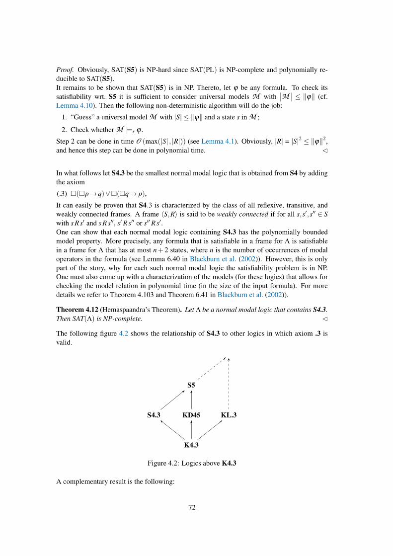
Proof. Obviously, SAT(S5) is NP-hard since SAT(PL) is NP-complete and polynomially re-ducible to SAT(S5).It remains to be shown that SAT(S5) is in NP. Thereto, let ϕ be any formula. To check itssatisfiability wrt. S5 it is sufficient to consider universal models M with

∣∣M ∣∣ ≤ ‖ϕ‖ (cf.Lemma 4.10). Then the following non-deterministic algorithm will do the job:

1. “Guess” a universal model M with |S| ≤ ‖ϕ‖ and a state s in M ;

2. Check whether M |=s ϕ .

Step 2 can be done in time O (max(|S| , |R|)) (see Lemma 4.1). Obviously, |R| = |S|2 ≤ ‖ϕ‖2,and hence this step can be done in polynomial time. C

In what follows let S4.3 be the smallest normal modal logic that is obtained from S4 by addingthe axiom

(.3) �(�p→q)∨�(�q→ p),

It can easily be proven that S4.3 is characterized by the class of all reflexive, transitive, andweakly connected frames. A frame 〈S,R〉 is said to be weakly connected if for all s,s′,s′′ ∈ Swith s R s′ and s R s′′, s′ R s′′ or s′′ R s′.One can show that each normal modal logic containing S4.3 has the polynomially boundedmodel property. More precisely, any formula that is satisfiable in a frame for Λ is satisfiablein a frame for Λ that has at most n+ 2 states, where n is the number of occurrences of modaloperators in the formula (see Lemma 6.40 in Blackburn et al. (2002)). However, this is onlypart of the story, why for each such normal modal logic the satisfiability problem is in NP.One must also come up with a characterization of the models (for these logics) that allows forchecking the model relation in polynomial time (in the size of the input formula). For moredetails we refer to Theorem 4.103 and Theorem 6.41 in Blackburn et al. (2002)).

Theorem 4.12 (Hemaspaandra’s Theorem). Let Λ be a normal modal logic that contains S4.3.Then SAT(Λ) is NP-complete. C

The following figure 4.2 shows the relationship of S4.3 to other logics in which axiom .3 isvalid.

K4.3

S4.3 KD45

S5

KL.3

Figure 4.2: Logics above K4.3

A complementary result is the following:

72

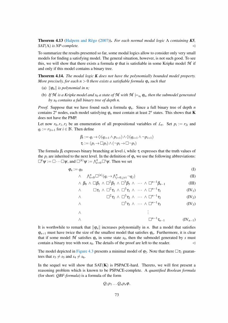
Theorem 4.13 (Halpern and Rego (2007)). For each normal modal logic Λ containing K5,SAT(Λ) is NP-complete. C

To summarize the results presented so far, some modal logics allow to consider only very smallmodels for finding a satisfying model. The general situation, however, is not such good. To seethis, we will show that there exists a formula ϕ that is satisfiable in some Kripke model M ifand only if this model contains a binary tree.

Theorem 4.14. The modal logic K does not have the polynomially bounded model property.More precisely, for each n > 0 there exists a satisfiable formula ϕn such that

(a) ‖ϕn‖ is polynomial in n;

(b) If M is a Kripke model and s0 a state of M with M |=s0 ϕn, then the submodel generatedby s0 contains a full binary tree of depth n.

Proof. Suppose that we have found such a formula ϕn. Since a full binary tree of depth ncontains 2n nodes, each model satisfying ϕn must contain at least 2n states. This shows that Kdoes not have the PMP.Let now r0,r1,r2 be an enumeration of all propositional variables of Lτ . Set pi := r2i andqi := r2i+1 for i ∈N. Then define

βi := qi→♦(qi+1∧ pi+1)∧♦(qi+1∧¬pi+1)

τi := (pi→�pi)∧ (¬pi→�¬pi)

The formula βi expresses binary branching at level i, while τi expresses that the truth values ofthe pi are inherited to the next level. In the definition of ϕn we use the following abbreviations:�kψ :=� · · ·�ψ , and �(k)ψ :=

∧ki=0�

iψ . Then we set

ϕn := q0 (I)

∧∧n

i=0�(n)(qi→

∧nj=0, j 6=i¬q j) (II)

∧ β0 ∧ �β1 ∧ �2β2 ∧ �3

β3 ∧ ·· · ∧ �n−1βn−1 (III)

∧ �τ1 ∧ �2τ1 ∧ �3

τ1 ∧ ·· · ∧ �n−1τ1 (IV1)

∧ �2τ2 ∧ �3

τ2 ∧ ·· · ∧ �n−1τ2 (IV2)

∧ �3τ3 ∧ ·· · ∧ �n−1

τ3 (IV3)

∧...

∧ �n−1τn−1 (IVn−1)

It is worthwhile to remark that ‖ϕn‖ increases polynomially in n. But a model that satisfiesϕn+1 must have twice the size of the smallest model that satisfies ϕn. Furthermore, it is clearthat if some model M satisfies ϕn in some state s0, then the submodel generated by s mustcontain a binary tree with root s0. The details of the proof are left to the reader. C

The model depicted in Figure 4.3 presents a minimal model of ϕ2. Note that there �τ1 guaran-tees that s3 6= s5 and s4 6= s6.

In the sequel we will show that SAT(K) is PSPACE-hard. Thereto, we will first present areasoning problem which is known to be PSPACE-complete. A quantified Boolean formula(for short: QBF-formula) is a formula of the form

Q1 p1 . . .Qn pnϕ,

73

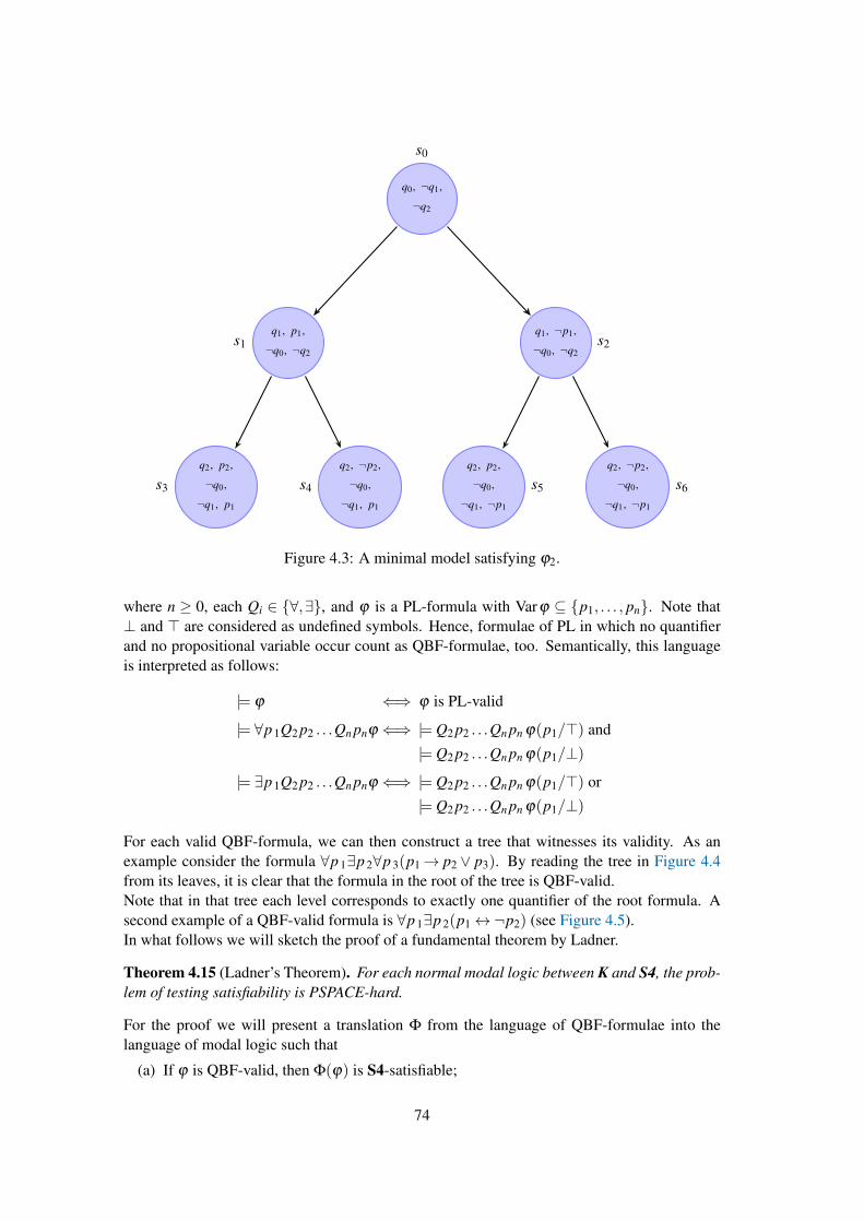
q0, ¬q1,

¬q2

s0

q1, p1,

¬q0, ¬q2s1

q2, p2,

¬q0,

¬q1, p1

s3

q2, ¬p2,

¬q0,

¬q1, p1

s4

q1, ¬p1,

¬q0, ¬q2s2

q2, p2,

¬q0,

¬q1, ¬p1

s5

q2, ¬p2,

¬q0,

¬q1, ¬p1

s6

Figure 4.3: A minimal model satisfying ϕ2.

where n ≥ 0, each Qi ∈ {∀,∃}, and ϕ is a PL-formula with Varϕ ⊆ {p1, . . . , pn}. Note that⊥ and > are considered as undefined symbols. Hence, formulae of PL in which no quantifierand no propositional variable occur count as QBF-formulae, too. Semantically, this languageis interpreted as follows:

|= ϕ ⇐⇒ ϕ is PL-valid

|= ∀p 1Q2 p2 . . .Qn pnϕ ⇐⇒ |= Q2 p2 . . .Qn pn ϕ(p1/>) and

|= Q2 p2 . . .Qn pn ϕ(p1/⊥)

|= ∃p 1Q2 p2 . . .Qn pnϕ ⇐⇒ |= Q2 p2 . . .Qn pn ϕ(p1/>) or

|= Q2 p2 . . .Qn pn ϕ(p1/⊥)

For each valid QBF-formula, we can then construct a tree that witnesses its validity. As anexample consider the formula ∀p 1∃p 2∀p 3(p1→ p2 ∨ p3). By reading the tree in Figure 4.4from its leaves, it is clear that the formula in the root of the tree is QBF-valid.Note that in that tree each level corresponds to exactly one quantifier of the root formula. Asecond example of a QBF-valid formula is ∀p 1∃p 2(p1↔¬p2) (see Figure 4.5).In what follows we will sketch the proof of a fundamental theorem by Ladner.

Theorem 4.15 (Ladner’s Theorem). For each normal modal logic between K and S4, the prob-lem of testing satisfiability is PSPACE-hard.

For the proof we will present a translation Φ from the language of QBF-formulae into thelanguage of modal logic such that

(a) If ϕ is QBF-valid, then Φ(ϕ) is S4-satisfiable;

74

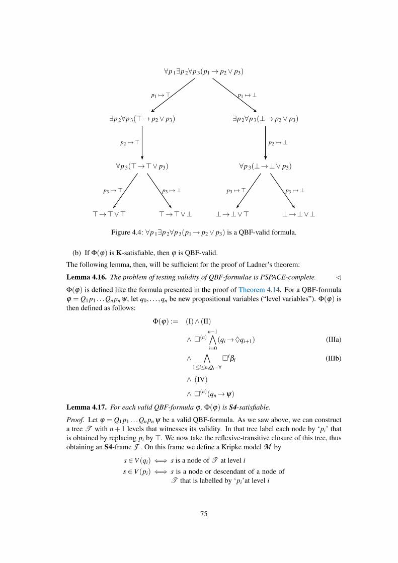
∀p 1∃p 2∀p 3(p1→ p2∨ p3)

∃p 2∀p 3(>→ p2∨ p3)

∀p 3(>→>∨ p3)

>→>∨>

p3 7→ >

>→>∨⊥

p3 7→ ⊥

p2 7→ >

p1 7→ >

∃p 2∀p 3(⊥→ p2∨ p3)

∀p 3(⊥→⊥∨ p3)

⊥→⊥∨>

p3 7→ >

⊥→⊥∨⊥

p3 7→ ⊥

p2 7→ ⊥

p1 7→ ⊥

Figure 4.4: ∀p 1∃p 2∀p 3(p1→ p2∨ p3) is a QBF-valid formula.

(b) If Φ(ϕ) is K-satisfiable, then ϕ is QBF-valid.

The following lemma, then, will be sufficient for the proof of Ladner’s theorem:

Lemma 4.16. The problem of testing validity of QBF-formulae is PSPACE-complete. C

Φ(ϕ) is defined like the formula presented in the proof of Theorem 4.14. For a QBF-formulaϕ = Q1 p1 . . .Qn pn ψ , let q0, . . . ,qn be new propositional variables (“level variables”). Φ(ϕ) isthen defined as follows:

Φ(ϕ) := (I)∧ (II)

∧ �(n)n−1∧i=0

(qi→♦qi+1) (IIIa)

∧∧

1≤i≤n,Qi=∀�i

βi (IIIb)

∧ (IV)

∧ �(n)(qn→ψ)

Lemma 4.17. For each valid QBF-formula ϕ , Φ(ϕ) is S4-satisfiable.

Proof. Let ϕ = Q1 p1 . . .Qn pn ψ be a valid QBF-formula. As we saw above, we can constructa tree T with n+ 1 levels that witnesses its validity. In that tree label each node by ‘pi’ thatis obtained by replacing pi by >. We now take the reflexive-transitive closure of this tree, thusobtaining an S4-frame F . On this frame we define a Kripke model M by

s ∈V (qi) ⇐⇒ s is a node of T at level i

s ∈V (pi) ⇐⇒ s is a node or descendant of a node ofT that is labelled by ‘pi’at level i

75

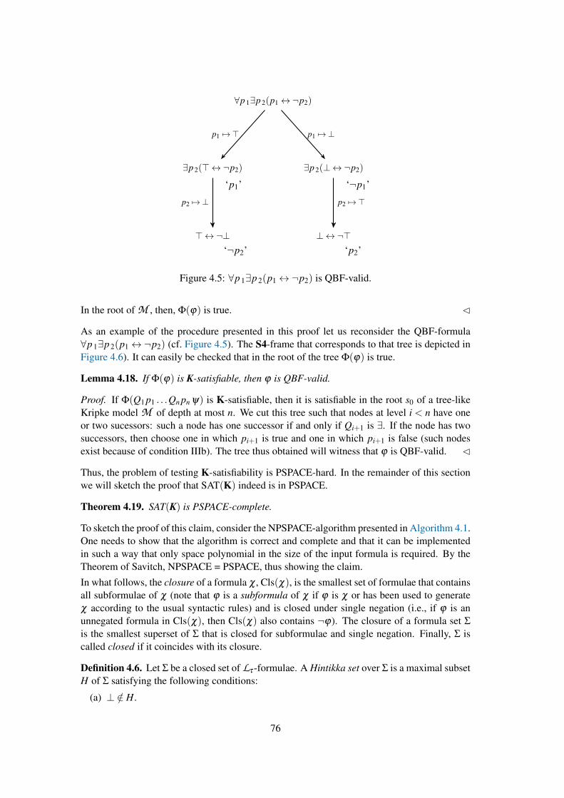
∀p 1∃p 2(p1↔¬p2)

∃p 2(>↔¬p2)

‘p1’

>↔¬⊥‘¬p2’

p2 7→ ⊥

p1 7→ >

∃p 2(⊥↔¬p2)

‘¬p1’

⊥↔¬>‘p2’

p2 7→ >

p1 7→ ⊥

Figure 4.5: ∀p 1∃p 2(p1↔¬p2) is QBF-valid.

In the root of M , then, Φ(ϕ) is true. C

As an example of the procedure presented in this proof let us reconsider the QBF-formula∀p 1∃p 2(p1↔¬p2) (cf. Figure 4.5). The S4-frame that corresponds to that tree is depicted inFigure 4.6). It can easily be checked that in the root of the tree Φ(ϕ) is true.

Lemma 4.18. If Φ(ϕ) is K-satisfiable, then ϕ is QBF-valid.

Proof. If Φ(Q1 p1 . . .Qn pn ψ) is K-satisfiable, then it is satisfiable in the root s0 of a tree-likeKripke model M of depth at most n. We cut this tree such that nodes at level i < n have oneor two sucessors: such a node has one successor if and only if Qi+1 is ∃. If the node has twosuccessors, then choose one in which pi+1 is true and one in which pi+1 is false (such nodesexist because of condition IIIb). The tree thus obtained will witness that ϕ is QBF-valid. C

Thus, the problem of testing K-satisfiability is PSPACE-hard. In the remainder of this sectionwe will sketch the proof that SAT(K) indeed is in PSPACE.

Theorem 4.19. SAT(K) is PSPACE-complete.

To sketch the proof of this claim, consider the NPSPACE-algorithm presented in Algorithm 4.1.One needs to show that the algorithm is correct and complete and that it can be implementedin such a way that only space polynomial in the size of the input formula is required. By theTheorem of Savitch, NPSPACE = PSPACE, thus showing the claim.

In what follows, the closure of a formula χ , Cls(χ), is the smallest set of formulae that containsall subformulae of χ (note that ϕ is a subformula of χ if ϕ is χ or has been used to generateχ according to the usual syntactic rules) and is closed under single negation (i.e., if ϕ is anunnegated formula in Cls(χ), then Cls(χ) also contains ¬ϕ). The closure of a formula set Σ

is the smallest superset of Σ that is closed for subformulae and single negation. Finally, Σ iscalled closed if it coincides with its closure.

Definition 4.6. Let Σ be a closed set of Lτ -formulae. A Hintikka set over Σ is a maximal subsetH of Σ satisfying the following conditions:

(a) ⊥ /∈ H.

76

¬p1,

¬p2, q0,

¬q1, ¬q2

s0

p1, ¬p2,

q1, ¬q0,

¬q2

s1

p1, ¬p2,

¬q0,

¬q1, q2

s3

¬p1,

¬p2, ¬q0,

q1, ¬q2

s2

¬p1,

p2, ¬q0,

¬q1, q2

s4

Figure 4.6: S4-model associated with the QBF-formula ∀p 1∃p 2(p1↔¬p2).

(b) For each ¬ϕ ∈ Σ, ¬ϕ ∈ H if and only if ϕ /∈ H;

(c) For each (ϕ ∧ψ) ∈ Σ, (ϕ ∧ψ) ∈ H if and only if ϕ ∈ H and ψ ∈ H.

Note that Hintikka sets need not be satisfiable. Moreover, a formula ϕ is satisfiable if and onlyif there exists a satisfiable Hintikka set H over Cls(ϕ) that contains ϕ .Without proving it here, we mention (for the proof, see Lemma 6.46 in Blackburn et al. (2002)):

Lemma 4.20. A Hintikka set H is satisfiable (in some Kripke model) if and only if it is satisfi-able in a finite tree-like model of depth at most max({depthϕ : ϕ ∈ H}).

The interesting aspect is that the “shallow” tree model mentioned in the lemma can be con-structed from a system H of Hintikka sets that has the following properties: (a) H ∈H ; (b) forall H ′ ∈H and ♦ψ ∈H ′, there exists an H ′′ ∈H that such that {χ : �χ ∈H ′}∪{ψ} ⊆H ′′;and (c) for each H ′ ∈H there exists a “chain” H = H0, . . . ,Hn = H ′ ∈H such that for each0 ≤ i < n, {χ : �χ ∈ Hi}∪{ψi} ⊆ Hi+1 for some ♦ψi ∈ Hi. This fact can be used to showthe correctness of Algorithm 4.1. Note that all sets of formulae occurring while executing thealgorithm are subsets of Cls(ϕ) and hence have an encoding polynomial in the size of ϕ (forexample, if ϕ is represented by its syntax tree, a set of subformulae can be represented by alist of pointers to nodes in that tree). Moreover, each assignment to Σψ (line 12) reduces the

77

Algorithm 4.1 SAT/WITNESS-Algorithm

procedure SAT(ϕ)inputs: ϕ , a formula of Kreturns: true or false

guess a set H ⊆ Cls(ϕ) with ϕ ∈ H5: return WITNESS(H,ϕ)

procedure WITNESS(H,Σ)inputs: H,Σ, finite sets of formulaereturns: true (if H is a satisfiable Hintikka set over Cls(Σ)) or false (otherwise)

if H is not a Hintikka set over Cls(Σ) then10: return false

for ♦ψ ∈ H doset Σψ := {χ : �χ ∈ H}∪{ψ}guess a subset Hψ with Σψ ⊆ Hψ ⊆ Cls(Σψ)if WITNESS(Hψ ,Σψ) = false then

15: return falsereturn true

Table 4.1: Complexity of the satisfiability problem for selected modal logics

K, KD, KT,KB, KDB K4, KD4, S4 K5, KD5, KB5,

K45, KD45, S5general PSPACE-cmpl PSPACE-cmpl NP-cmpldepth≤ k NP-cmpl PSPACE-cmpl NP-cmpldepth = 1 NP-cmpl NP-cmpl NP-cmpl

maximal modal depth of the formulae sets that are used as input for the next recursive callof the WITNESS procedure. Thus, the recursion depth is bounded by the maximal depth of aformula in Cls(ϕ) and hence by the size of ϕ .

Remark 4.2. Even if the complexity of the general satisfiability problem is PSPACE-hard formany modal logics, it is often the case that we get tighter complexity bounds when we imposerestrictions on the formulae that are to be checked for satisfiability (Ladner, 1977; Halpern,1995; Nguyen, 2004). Remark 4.3 gives some overview.

Remark 4.3. For multi-modal languages the complexity of reasoning problems may increaseconsiderably.

• For n > 1 the satisfiability problem for S5n and KD45n is PSPACE-complete (rememberthat for n = 1 the satisfiability problem for these logics is NP-complete).

• If the system K is extended by a further diamond operator which is interpreted by the uni-versal relation, then for the resulting system the satisfiability problem shifts from PSPACEto EXPTIME.

78

• Later we will discuss a system that allows for modeling common knowledge of n agents.However, by adding common knowledge to one of the systems K4n, S4n, KD45n, or S5n,the complexity of the satisfiability problem increases from PSPACE to EXPTIME, thoughthe resulting system still has the finite model property.

79

80

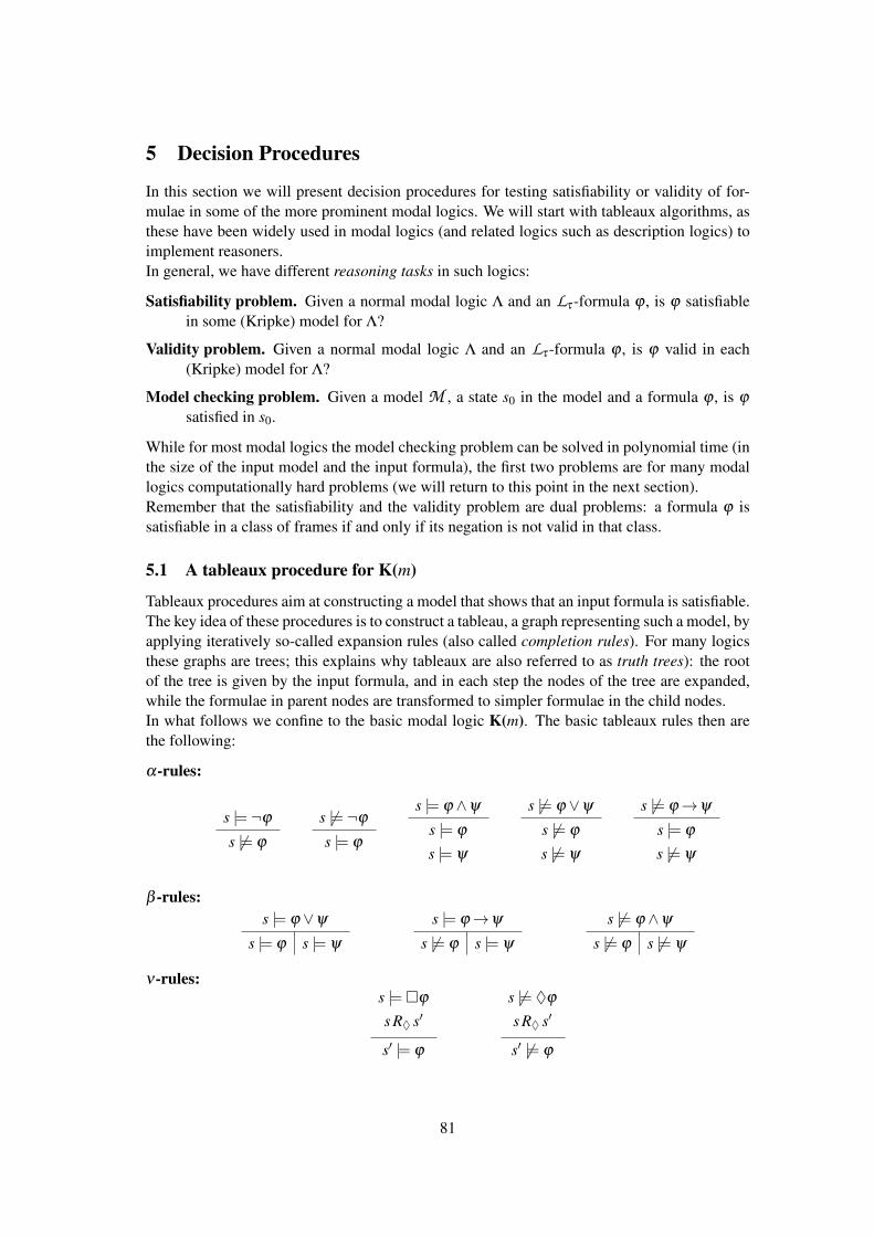
5 Decision Procedures

In this section we will present decision procedures for testing satisfiability or validity of for-mulae in some of the more prominent modal logics. We will start with tableaux algorithms, asthese have been widely used in modal logics (and related logics such as description logics) toimplement reasoners.In general, we have different reasoning tasks in such logics:

Satisfiability problem. Given a normal modal logic Λ and an Lτ -formula ϕ , is ϕ satisfiablein some (Kripke) model for Λ?

Validity problem. Given a normal modal logic Λ and an Lτ -formula ϕ , is ϕ valid in each(Kripke) model for Λ?

Model checking problem. Given a model M , a state s0 in the model and a formula ϕ , is ϕ

satisfied in s0.

While for most modal logics the model checking problem can be solved in polynomial time (inthe size of the input model and the input formula), the first two problems are for many modallogics computationally hard problems (we will return to this point in the next section).Remember that the satisfiability and the validity problem are dual problems: a formula ϕ issatisfiable in a class of frames if and only if its negation is not valid in that class.

5.1 A tableaux procedure for K(m)

Tableaux procedures aim at constructing a model that shows that an input formula is satisfiable.The key idea of these procedures is to construct a tableau, a graph representing such a model, byapplying iteratively so-called expansion rules (also called completion rules). For many logicsthese graphs are trees; this explains why tableaux are also referred to as truth trees): the rootof the tree is given by the input formula, and in each step the nodes of the tree are expanded,while the formulae in parent nodes are transformed to simpler formulae in the child nodes.In what follows we confine to the basic modal logic K(m). The basic tableaux rules then arethe following:

α-rules:

s |= ¬ϕ

s 6|= ϕ

s 6|= ¬ϕ

s |= ϕ

s |= ϕ ∧ψ

s |= ϕ

s |= ψ

s 6|= ϕ ∨ψ

s 6|= ϕ

s 6|= ψ

s 6|= ϕ→ψ

s |= ϕ

s 6|= ψ

β -rules:s |= ϕ ∨ψ

s |= ϕ s |= ψ

s |= ϕ→ψ

s 6|= ϕ s |= ψ

s 6|= ϕ ∧ψ

s 6|= ϕ s 6|= ψ

ν-rules:s |=�ϕ

s R♦ s′

s′ |= ϕ

s 6|= ♦ϕ

s R♦ s′

s′ 6|= ϕ

81

π-rules:s 6|=�ϕ

s R♦ s′

s′ 6|= ϕ

where s′ is a freshstate name

s |= ♦ϕ

s R♦ s′

s′ |= ϕ

where s′ is a freshstate name

As can be seen from the rules, we are considering “state-labelled” formulae of the form s |= ϕ

and s 6|= ϕ , where s is a state name and ϕ is a modal-logical formula. Starting from a state-labelled formula (the input formula that is to be tested for satisfiability labelled with an arbitrarystate name), one iteratively applies these rules on the branches of the tree so-far constructed:a rule may be applied on a branch, when every antecedent of the rule occurs in the branch. Abranch is closed if it contains a clash, i.e., state-labelled formulae s |= ϕ and s 6|= ϕ . Non-closedbranches are called open. A branch is finished if no rule can be applied on it. An open branchthat contains state-labelled formulae s |= p or s 6|= p for each propositional variable p occurringin the root formula defines a Kripke model that makes the statement of the root formula true.So if the root is of the form s |= ϕ , the open branch defines a Kripke model in which ϕ is true atstate s: this shows that ϕ is satisfiable. If the root is of the form s 6|= ϕ , the open branch gives acounterexample showing that ϕ is not valid. Hence in order to prove that a formula ϕ is valid,one tries to find a counterexample by developing the tableau of s 6|= ϕ . When each branch isclosed, the formula is indeed valid; otherwise, it is not.

Remark 5.1. α- and β -rules handle the propositional-logical connectives. α-rules are deter-ministic rules: applying one of them on a branch in a tableau, they just expand the currentbranch. Contrary to this, β -rules are non-deterministic, i.e., they generate alternative childnodes and thus alternative completions of the current branch. We will see that both α- andβ -rules need to be applied only once. ν- and π-rules handle the modal-logical connectives.ν-rules are also deterministic rules, but it may be necessary to apply them more than one timeon a state-labelled formula s |= �ϕ (or s 6|= ♦ϕ) occurring in the current branch. π-rules arealso deterministic (given a fixed sequence of “unused” state names), but need to be appliedonly once.

Examples of tableaux proofs are presented in Figures 5.1 – 5.3. The first example is a simple,propositional logic example: the tableau proves that the formula p→ (q→ (p∧q)) is valid inK(m). The second example shows that axiom K is valid and the third example shows that theformula ♦p∧♦q→♦(p∧q) is not valid.

The idea of the (semantic) tableaux method presented above is to construct Kripke models.In order to make this explicit, we introduce the notion of completion trees (which represent“partial” Kripke models) and reformulate the tableaux rules in a way that shows how the rulesmodify these trees. For the sake of simplicity we make the following assumptions: (a) weassume a setting in which ¬,∧,∨,♦i,�i (1 ≤ i ≤ m) are chosen as syntactic primitives; and(b) we assume that the formulae that are input to the tableaux procedure are in negation normalform, i.e., the negation symbol occurs only in front of propositional variables.Remember that the closure of a formula χ , Cls(χ), is the smallest set of formulae that containsall subformulae of χ and is closed under “single” negation (i.e., if ϕ is an unnegated formulain Cls(χ), then Cls(χ) also contains ¬ϕ).

Definition 5.1. A completion tree for a formula χ is a (vertex- and edge-labeled) graph Gχ =〈V,A,L〉, where V is a set of vertices, A is a set of arcs on V (i.e., A ⊆V 2), and L is a labeling

82

s0 6|= p→ (q→ (p∧q))

s0 |= p

s0 6|= q→ (p∧q)

s0 |= q

s0 6|= p∧q

s0 6|= p s0 6|= q

X X

Figure 5.1: An example of a propositional logic tableau

s0 6|=�(p→q)→ (�p→�q)

s0 |=�(p→q)

s0 6|=�p→�q

s0 |=�p

s0 6|=�q

s0 R♦ s1

s1 6|= q

s1 |= p→q

s1 |= p

s1 6|= p s1 |= q

X X

Figure 5.2: Tableau proof of axiom K

83

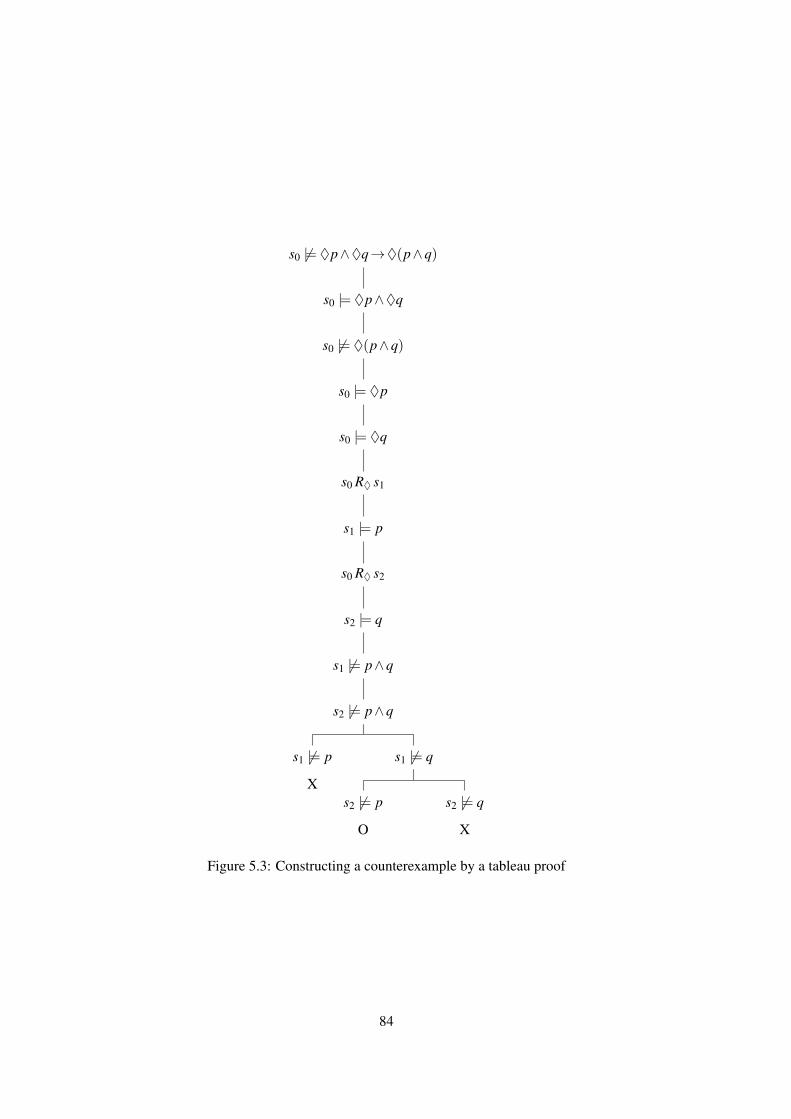
s0 6|= ♦p∧♦q→♦(p∧q)

s0 |= ♦p∧♦q

s0 6|= ♦(p∧q)

s0 |= ♦p

s0 |= ♦q

s0 R♦ s1

s1 |= p

s0 R♦ s2

s2 |= q

s1 6|= p∧q

s2 6|= p∧q

s1 6|= p s1 6|= q

s2 6|= p s2 6|= qX

O X

Figure 5.3: Constructing a counterexample by a tableau proof

84

function that assigns to each v ∈V a set L(v)⊆ Cls(χ) and to each arc a = (v,v′) ∈ A a naturalnumber L(a) ∈ {1, . . . ,m}.

Given a completion tree 〈V,A,L〉, we can reformulate the tableaux rules for our syntactic settingas described in the following definition.

Definition 5.2. The tableaux rules for K(m) are the following:

∧-rule. If ϕ ∧ψ ∈ L(v) and {ϕ,ψ} 6⊆ L(v), then set L(v)← L(v)∪{ϕ,ψ}.

∨-rule. If ϕ ∨ψ ∈ L(v) and {ϕ,ψ} ∩ L(v) = /0, then set L(v)← L(v)∪ {ϕ} or set L(v)←L(v)∪{ψ}.

♦-rule. If ♦iϕ ∈ L(v) and there is no v′ ∈ V with (v,v′) ∈ A, L(v,v′) = i, and ϕ ∈ L(v′), thenextend V by a fresh node v∗ and set A← A∪{(v,v∗)}, L(v∗)←{ϕ}, and L(v,v∗)← i.

�-rule. If�iϕ ∈ L(v) and there is some v′ ∈V with (v,v′)∈ A, L(v,v′) = i, and ϕ /∈ L(v′), thenset L(v′)← L(v′)∪{ϕ}.

Definition 5.3. A completion tree G = 〈V,A,L〉 is said to be clash-free if there is no v∈V suchthat {p,¬p} ⊆ L(v) for some propositional variable p. A completion tree is called completeif none of the completion rules presented in Definition 5.2 can be applied. A complete andclash-free completion tree is also often referred to as tableau.

We say that a completion tree 〈V,A,L〉 is satisfiable if there exists a Kripke model M with frame〈S,{R♦i}1≤i≤m〉 such that V ⊆ S, {a ∈ A : L(a) = i} ⊆ R♦i (1 ≤ i ≤ m), and M |=v L(v) foreach v∈V . Note that for the definition of the model it is sufficient to interpret the propositionalvariables that occur in the closure of the input formula.

Lemma 5.1.(a) A completion tree G is satisfiable if and only if one of the completion trees resulting from

applying any K(m) tableaux rule on G is satisfiable.

(b) A completion tree that contains a clash is not satisfiable.

(c) If a completion tree 〈V ′,A′,L′〉 is complete and clash-free, then

S :=V ′, R♦i := {a ∈ A′ : L′(a) = i}, V (p) := {s ∈ S : p ∈ L′(s)}

defines a Kripke model M that trivially satisfies M |=s L′(s) for each state s. C

In what follows we describe the tableaux procedure in more detail. Algorithm 5.1 provides arather sketchy version that closely reflects the basic idea: apply the tableaux rules on the initialcompletion tree that is given by the input formula. If a clash is detected in the completiontree, we return unsatisfiable; if the completion tree is clash-free and complete, we have founda Kripke model that satisfies the completion tree and hence also satisfies the completion treedefined by the input formula of the procedure. If the completion tree is clash-free, but not com-plete, we can apply further rules and then check the satisfiability of the modified completiontree. Note that this algorithm is non-deterministic. For proving its correctness we may assumethat (when possible) the right choice is made whenever the ∨-rule is applied.

Remark 5.2. Notice that a non-deterministic Turing machine accepts a word if at least onecomputation on the input word results in an accepting state. It should be noted that the

85

Algorithm 5.1 CHECKSAT (non-deterministic version)

procedure CHECKSAT(ϕ)inputs: ϕ , a formula of K(m) in NNFreturns: satisfiable or unsatisfiable

V ←{v0} , A← /0 , L(v0)←{ϕ}5: return COMPLETETREE(〈V,A,L〉)

procedure COMPLETETREE(G)inputs: G, a completion treereturns: satisfiable or unsatisfiable

if G contains a clash then10: return unsatisfiable

if G is complete thenreturn satisfiable

G← apply some completion rule on some formula in Greturn COMPLETETREE(G)

non-deterministic version of the CHECKSAT algorithm involves different versions of non-determinism. First, with regard to correctness of the algorithm, it is irrelevant which rule isapplied in each step (“don’t care” non-determinism). Contrary to that, it is essential whichchoice is made when the ∨-rule is applied (“don’t know” non-determinism).

Algorithm 5.2 provides a deterministic version. It uses two auxiliary functions: SELECTFOR-MULA selects a formula from one of the label sets L(v) in the completion tree that is not a literal(a literal is a formula of the form p or ¬p where p is a propositional variable); to avoid earlybranching, it is in most cases reasonable to defer the selection of an ∨-formula or a ♦-formulaas long as possible. APPLYRULE takes as input a completion tree, a vertex in that tree, and aformula (on which a rule can be applied) and returns the list of completion trees that result fromapplying an appropriate rule (as listed in Definition 5.2); in the case of the ∧-, �-, or ♦-rulethe resulting list consists of a single completion tree and in the case of the ∨-rule it consists oftwo completion trees (one for each choice).The search for a tableau for an input formula starts with an initial completion tree with ex-actly one vertex v0 that has a singleton label set containing the input formula. On this initialcompletion tree we execute the procedure COMPLETETREE, which searches for a clash-freeand complete completion of the input tree in depth-first manner. On an input completion treeCOMPLETETREE first checks, whether the completion tree is clash-free and whether still rulescan be applied on a formula occurring in one of the label sets. When we have found a clash, weneed to backtrack. If we have found a clash-free and complete completion tree, we are finishedand thus the algorithm returns “satisfiable”. Otherwise, we select one of the formulae on whichrules can be applied, generate a list of possible completion trees, and execute in a recursivemanner on each of these trees COMPLETETREE. Note that in each recursive call, COMPLETE-TREE operates on a completion tree in which some label set will contain new formulae ofsmaller degree. Thus, eventually we will end up with a completion tree in which no rule canbe applied any more (on any vertex introduced earlier into the completion tree). This showsthat COMPLETETREE will not generate an infinite sequence of completion trees in which eachresults from its predecessor by applying a rule. That is, termination of the tableaux procedure

86

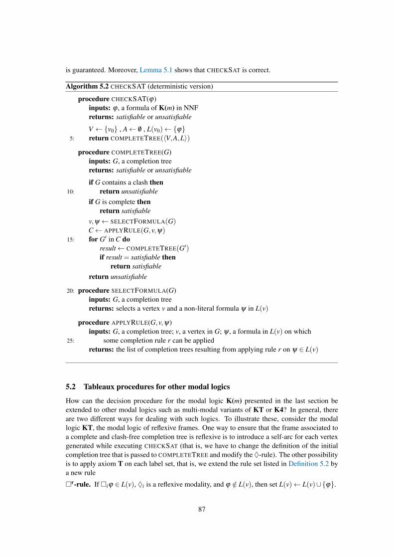
is guaranteed. Moreover, Lemma 5.1 shows that CHECKSAT is correct.

Algorithm 5.2 CHECKSAT (deterministic version)

procedure CHECKSAT(ϕ)inputs: ϕ , a formula of K(m) in NNFreturns: satisfiable or unsatisfiable

V ←{v0} , A← /0 , L(v0)←{ϕ}5: return COMPLETETREE(〈V,A,L〉)

procedure COMPLETETREE(G)inputs: G, a completion treereturns: satisfiable or unsatisfiable

if G contains a clash then10: return unsatisfiable

if G is complete thenreturn satisfiable

v,ψ ← SELECTFORMULA(G)C← APPLYRULE(G,v,ψ)

15: for G′ in C doresult← COMPLETETREE(G′)if result = satisfiable then

return satisfiablereturn unsatisfiable

20: procedure SELECTFORMULA(G)inputs: G, a completion treereturns: selects a vertex v and a non-literal formula ψ in L(v)

procedure APPLYRULE(G,v,ψ)inputs: G, a completion tree; v, a vertex in G; ψ , a formula in L(v) on which

25: some completion rule r can be appliedreturns: the list of completion trees resulting from applying rule r on ψ ∈ L(v)

5.2 Tableaux procedures for other modal logics

How can the decision procedure for the modal logic K(m) presented in the last section beextended to other modal logics such as multi-modal variants of KT or K4? In general, thereare two different ways for dealing with such logics. To illustrate these, consider the modallogic KT, the modal logic of reflexive frames. One way to ensure that the frame associated toa complete and clash-free completion tree is reflexive is to introduce a self-arc for each vertexgenerated while executing CHECKSAT (that is, we have to change the definition of the initialcompletion tree that is passed to COMPLETETREE and modify the♦-rule). The other possibilityis to apply axiom T on each label set, that is, we extend the rule set listed in Definition 5.2 bya new rule

�r-rule. If �iϕ ∈ L(v), ♦i is a reflexive modality, and ϕ /∈ L(v), then set L(v)← L(v)∪{ϕ}.

87

Moreover, the Kripke model associated to a complete and clash-free completion tree needs tobe adapted: Given such a completion tree, the accessibility relation of a reflexive modality ♦i isnot just the set of arcs a with L(a) = i, but the reflexive closure of this set. The main advantageof the latter method is that we preserve a tree structure of completion “trees”.

While extending the tableaux procedure on reflexive modalities is simple, the case of transitivemodalities is more involved. The reason for this is that a naive extension will lead to a non-terminating procedure. As an example consider the formula ♦p∧�(p→♦p) where ♦ is atransitive modality. By applying the ♦-rule on ♦p ∈ L(v), we will generate a new vertex v′

with L(v′) = {p}. When we apply the �-rule on �(p→♦p) ∈ L(v), we need to extend L(v′)by p→♦p and hence eventually by ♦p. Thus we will add a new vertex v′′ to the completiontree (a successor of v′) with L(v′′) = {p}. By “transitivity” (in either of the ways describedabove implemented), we will extend L(v′′) by the formula p→♦p and thus we will need tointroduce a further vertex, etc.This problem can be dealt with by a technique called blocking. The idea is to block the expan-sion of a completion tree whenever the process runs into a “loop”, that is, the newly generatedvertex together with its labels set contains only irrelevant information that is already encodedin its parent vertex or somewhere else in the completion tree. In the case of transitivity, theblocking condition is as follows: A vertex v is said to block v′ if L(v′)⊆ L(v) (subset blocking)and v is called a witness for v′ (note that is not required that there is an (v,v′) ∈ A). Hence wehave a modified ♦-rule and an additional rule that employs axiom 4 to add further formulae to“neighbored” label sets.

♦’-rule. If (a) ♦iϕ ∈ L(v), (b) v is not blocked, and (c) there is no v′ ∈ V with (v,v′) ∈ A,L(v,v′) = i, and ϕ ∈ L(v′), then extend V by a fresh node v∗ and set A← A∪{(v,v∗)},L(v∗)←{ϕ}, and L(v,v∗)← i.

�+-rule. If (a) �iϕ ∈ L(v), (b) ♦i is a transitive modality, and (c) there is some v′ ∈ V with(v,v′) ∈ A, L(v,v′) = i, and �iϕ /∈ L(v′), then set L(v′)← L(v′)∪{�iϕ}.

Do these modifications guarantee termination? This is not clear in the general setting whereone considers more refined blocking conditions and/or does not fix the order in which rules areapplied. For example, it may happen that a blocked vertex is getting unblocked when furtherrules are applied on the parent vertex that modify the blocked vertex in such a way that theblocking condition does no longer hold (dynamic blocking). For this reason it makes sense todefer the execution of the generating ♦-rule on a vertex until no non-generating rule can beapplied any more on any available vertex in the completion tree (static blocking). Moreover, ifno rule is applied that modifies the label set of a blocking vertex, a blocked vertex cannot getunblocked any more. This “strategy” of rule application ensures that no infinite sequence ofcompletion trees in which each tree results from its predecessor by some rule application canbe generated.

Lemma 5.2. Let G = 〈V,A,L〉 be a completion tree for a formula χ and nχ = |Cls(χ)|.(a) Let G′ be the result of applying one of the completion rules on G under the static blocking

strategy. If v′ is blocked by v in G, then it is also blocked by v in G′.

(b) IfV contains more than 2nχ elements, then there exist v,v′ ∈V with L(v) = L(v′).

(c) Let G′ be the result of applying a finite number of completion rules on G under the staticblocking strategy. Then G′ contains at most 2nχ non-blocked vertices.

88

(d) Let G′ be any completion tree resulting from G by finitely many rule applications underthe static blocking strategy. Then the number of vertices in the completion tree G′ isbounded by 22·nχ .

Proof. (a) Obviously, each rule application can only monotonically add formulae to label setsof unblocked vertices (because of static blocking). Hence if L(v′)⊆ L(v) holds in G, this subsetrelation must be true in G′ as well.

(b) Since each L(v) is a subset of Cls(χ), there are at most 2nχ pairwise distinct label sets.

(c) If G′ contains more than 2nχ unblocked nodes, then there exist unblocked vertices v,v′ inG′ with L(v) = L(v′). Since all vertices are introduced in some order, we may assume that vhad been added to V before v′ was added. But this means that at some step vertex v blocks v′

(in contradiction to the assumption that v′ is unblocked): by (a), a blocked vertex cannot getunblocked by further rule applications under the static blocking strategy.

(d) In each finite sequence of rule applications we can only generate 2nχ non-blocked verticesin the completion tree. Under the given strategy, rules are only applied on these non-blockedvertices. Each non-blocked vertex can have at most 2nχ outgoing arcs in the completion tree(since label sets contain at most 2nχ formulae) and blocked vertices do not have outgoing arcs.This entails that the number of possibly introduced vertices in the completion tree is boundedby 2nχ ×2nχ = 22·nχ . C

5.3 Optimization techniques

In this section we describe some optimization techniques for tableaux procedures: these tech-niques aim at either improving search (for example, reduce the width of the search tree andskip irrelevant branching points when backtracking after a clash has been detected).

Semantic branching. The ∨-rule as given in Definition 5.2 performs syntactic branching:when it is applied on a disjunction ϕ ∨ψ ∈ L(v), one first checks whether, say, L(v)∪{ϕ}leads to a clash in the modified completion tree. If so, one continues with L(v)∪{ψ}. But thismeans that the information is lost that L(v)∪{ϕ} (and hence each superset of this label set)leads to a clash. To avoid this it is suggesting to continue with the label set L(v)∪{ψ,¬ϕ}(or: L(v)∪{ψ,NNF(¬ϕ)}) when the decision L(v)∪{ϕ} turns out to be unsatisfiable. Thistechnique is called semantic branching: it is based on the propositional logic equivalence (ϕ ∨ψ) ↔ (ϕ ∨ (¬ϕ ∧ψ)). A potential drawback of semantic branching is that adding ¬ϕ tothe label set increases the amount of formulae that need to be processed further on: suchformulae may be disjunctions or ♦-formulae and hence may lead to the generation of new, butunnecessary vertices in the completion tree or branching nodes during search.

Local simplification, Boolean constraint propagation. Local simplification methods aimat reducing the width of the search tree by simplifying formulae before non-deterministic com-pletion rules are applied. A special simplification method is Boolean constraint propagation:the idea is to use literals occurring in a label set in order to simplify in a deterministic waydisjunctions in such sets. For example, if a label set L(v) contains the formulae p∨ϕ and¬p, L(v) can be immediately extended by the formula ϕ . An example combining semanticbranching with Boolean constraint propagation is depicted in Figure 5.4. The benefit of suchpropagation techniques is that search space is never increased. A potential drawback is that inorder to use propagation techniques efficiently, more complex data structures for representing

89

formulae may be necessary. Horrocks (2003) reports that such techniques perform well on ran-domly generated problem instances, in particular on over-constrained instances that are likelyto be unsatisfiable.

Clash in L(v)

Clash in L(v)

L(v)←∪ {ϕ ∨ψ}L(v)←∪ {ϕ ∨χ}

L(v)←∪ {. . .}

L(v)←∪ {ϕ} L(v)←∪ {ψ}

L(v)←∪ {ϕ} L(v)←∪ {χ}

Clash in L(v)

L(v)←∪ {ϕ ∨ψ}L(v)←∪ {ϕ ∨χ}

L(v)←∪ {. . .}

L(v)←∪ {ϕ} L(v)←∪ {ψ,¬ϕ}

L(v)←∪ {χ}

Figure 5.4: Syntactic vs semantic branching (combined with Boolean constraint propagation)

Enhancements of backtracking search. As an alternative to the simple backtracking scheme,more sophisticated schemes have been discussed in the literature: a typical problem for back-tracking search is thrashing, i.e., search nodes are explored although they will not lead to a“solution”.An example of such an alternative backtracking scheme is dependency directed backjumping,initially developed in the CSP field. The main idea is to equip each search node with a setof search nodes it depends on. When during search we discover that the current search nodecannot lead to a solution, we do not just revise the last decision, but perform a backjump to thelast search node on which the current search node depends.In our context, in which the search nodes are given by completion trees, this basic idea can beimplemented as follows: each completion tree generated during search that has more than onesuccessor (decision node, branching node) is augmented with an identifier that is unique to thecurrently explored branch in the search tree. Furthermore, each formula in each label set aswell as each arc records the decision nodes it depends on: a formula ϕ ∈ L(v) is said to dependon a decision node n if ϕ has been added to L(v) at n or ϕ depends on another formula ψ ∈ L(v)that depends on n or an arc (v′,v)∈ A that depends on n. ϕ ∈ L(v) depends on ψ ∈ L(v) if ϕ hasbeen added to L(v) by applying some deterministic rule on ψ ∈ L(v). ϕ ∈ L(v) depends on anarc (v′,v) ∈ A if ϕ has been added to L(v) by applying some deterministic rule mentioning thisarc. An arc (v′,v) depends on a formula ψ ∈ L(v′) if v has been introduced by an applicationof the ♦-rule on ψ ∈ L(v′).During search we record these dependency relations. For example, if ϕ has been added to L(v)by applying the �-rule on ψ ∈ L(v′), the dependency set of ϕ ∈ L(v), denoted Dv(ϕ), will bethe union of the dependency sets of ψ ∈ L(v′) and of the arc (v′,v). If we apply the ♦-rule ona formula ♦ψ ∈ L(v) (thus generating a new node v∗), the dependency set of the arc (v,v∗) andthe dependency set of ψ ∈ L(v∗) both will be set to the dependency set of ♦ψ ∈ L(v).

90

Thus, if the search results in a completion tree with a clash {ϕ,¬ϕ} ⊆ L(v), we perform abackjump to the maximal member in the union of the dependency sets Dv(ϕ) and Dv(¬ϕ).Figure 5.5 presents an example: depicted is a part of the search tree when the tableaux proce-dure is processed on a formula of the form (p1∨q1)∧ (p2∨q2)∧♦ϕ ∧ (�(¬ϕ ∧ψ)∨ . . .).In general, dependency directed backjumping results in a significant simplification of the tra-versed search tree.

d0

d1

d2

d3

d4

Clash in L(v′)

L(v)←∪ {p1 ∨ q1}L(v)←∪ {p2 ∨ q2}

L(v)←∪ {♦ϕ}

Dv(p1 ∨q1) := {d0}Dv(p2 ∨q2) := {d0}

Dv(♦ϕ) := {d0}

L(v)←∪ {�(¬ϕ ∧ψ)}Dv(�(¬ϕ ∧ψ)) := {d1}

L(v)←∪ {. . .}Dv(. . .) := {d1}

L(v)←∪ {p1}Dv(p1) := {d2} L(v)←∪ {q1}

L(v)←∪ {p2}Dv(p2) := {d3} L(v)←∪ {q2}

V ←∪ {v∗}A←∪ {(v,v∗)}L(v∗)←∪ {ϕ}

D(v,v∗) := Dv(♦ϕ) = {d0}Dv∗ (ϕ) :=Dv(♦ϕ)= {d0}

L(v∗)←∪ {¬ϕ ∧ψ}Dv∗ (¬ϕ ∧ψ) :=

Dv(�(¬ϕ ∧ψ))∪D(v,v∗) = {d0,d1}Dv∗ (¬ϕ) := Dv∗ (¬ϕ ∧ψ)

jump back to maximal

element in Dv∗ (ϕ)∪Dv∗ (¬ϕ) = {d0,d1}

Figure 5.5: Dependency directed backjumping (Figure adapted from Horrocks (2003))

Search heuristics. Search heuristics aim at guiding search when decisions need to be made.In the context of the tableaux procedure heuristics come into play when one has to decidewhich disjunct in a disjunctive formula occurring in a label set is to be selected first. Onemethod (developed in the SAT field and applicable in the context of tableaux proofs as well) isthe so-called MOMS heuristic. The slogan of the MOMS heuristic is “select a formula that hasthe maximal number of occurrences in disjunctions of minimal size”. The MOMS heuristic

91

aims at optimizing Boolean constraint propagation: if such a disjunct leads to a clash, Booleanconstraint propagation will reduce the branching of subsequently explored search nodes.

The drawback of the MOMS heuristic is that it does not perform well in combination withdependency directed backjumping. Moreover, it may depend on the problem instances to besolved whether the MOMS heuristic provides useful information for selecting a disjunct.

Another search heuristic that is particularly useful in combination with dependency directedbackjumping is the oldest-first heuristic. The idea is here to use the dependency sets generatedduring search to select a disjunct that depends on the oldest decision node in the currentlyexpanded branch of the search tree. More precisely, one selects a disjunction that has theoldest element in its dependency set. Further heuristics can be combined with this heuristic toguide the selection of a disjunct in such a disjunction.

The benefit of using search heuristics is that they often can be combined efficiently with back-tracking schemes. Moreover, search heuristics may be selected dependent on the formula thatneeds to be processed.

92

References

Andreka, H., van Benthem, J., and Nemeti, I. (1995). Back and forth between modal logic andclassical logic. Logic Journal of the IGPL, 3(5):685–720.

Areces, C., de Rijke, M., and de Nivelle, H. (2001). Resolution in modal, description andhybrid logic. J. Log. Comput., 11(5):717–736.

Baader, F. and Nutt, W. (2003). Basic description logics. In Baader, F., Calvanese, D., McGuin-ness, D. L., Nardi, D., and Patel-Schneider, P. F., editors, Description Logic Handbook, pages43–95. Cambridge University Press.

Baader, F. and Sattler, U. (2001). An overview of tableau algorithms for description logics.Studia Logica, 69(1):5–40.

Blackburn, P., de Rijke, M., and Venema, Y. (2002). Modal Logic. Cambridge Tracks inTheoretical Computer Science. Cambridge University Press.

Buchheit, M., Donini, F. M., and Schaerf, A. (1993). Decidable reasoning in terminologicalknowledge representation systems. J. Artif. Intell. Res. (JAIR), 1:109–138.

Burgess, J. P. (1984). Basic tense logic. In Gabbay, D. and Guenthner, F., editors, Handbookof Philosophical Logic: Volume II: Extensions of Classical Logic, pages 89–133. Reidel,Dordrecht.

Chagrov, A. and Zakharyaschev, M. (1997). Modal Logic. Oxford University Press.

Chellas, B. F. (1980). Modal Logic: An Introduction. Cambridge University Press.

Clarke, E. M., Emerson, E. A., and Sistla, A. P. (1986). Automatic verification of finite-stateconcurrent systems using temporal logic specifications. ACM Trans. Program. Lang. Syst.,8(2):244–263.

Ebbinghaus, H.-D., Flum, J., and Thomas, W. (2007). Einfuhrung in die mathematische Logik(5. Aufl.). Spektrum Akademischer Verlag.

Emerson, E. A. (1990). Temporal and modal logic.

Fagin, R., Halpern, J. Y., Moses, Y., and Vardi, M. Y. (1995). Reasoning About Knowledge.MIT Press.

Fischer, M. J. and Ladner, R. E. (1977). Propositional modal logic of programs (extendedabstract). In STOC, pages 286–294. ACM.

Fitting, M. (1996). First-order logic and automated reasoning (2. ed.). Graduate texts incomputer science. Springer.

Gabbay, D., Kurucz, A., Wolter, F., and Zakharyaschev, M. (2003). Many-Dimensional ModalLogics: Theory and Applications. Elsevier.

Galton, A. (2008). Temporal logic. In Zalta, E. N., editor, The Stanford Encyclopedia ofPhilosophy. Fall 2008 edition.

93

Giunchiglia, F. and Sebastiani, R. (2000). Building decision procedures for modal logics frompropositional decision procedures: The case study of modal k(m). Inf. Comput., 162(1-2):158–178.

Goranko, V. and Otto, M. (2007). Model theory of modal logic. In Blackburn, P., Benthem,J. V., and Wolter, F., editors, Handbook of Modal Logic, pages 249–330. Elsevier.

Halpern, J. Y. (1995). The effect of bounding the number of primitive propositions and thedepth of nesting on the complexity of modal logic. Artif. Intell., 75(2):361–372.

Halpern, J. Y. and Rego, L. C. (2007). Characterizing the NP-PSPACE gap in the satisfiabilityproblem for modal logic. J. Log. Comput., 17(4):795–806.

Hintikka, J. (1962). Knowledge and Belief: An Introduction to the Logic of the Two Notions.Cornell University Press, Ithaca.

Hladik, J. (2002). Implementation and optimisation of a tableau algorithm for the guardedfragment. In Egly, U. and Fermuller, C. G., editors, TABLEAUX, volume 2381 of LectureNotes in Computer Science, pages 145–159. Springer.

Horrocks, I. (2003). Implementation and optimization techniques. In Baader, F., Calvanese,D., McGuinness, D. L., Nardi, D., and Patel-Schneider, P. F., editors, Description LogicHandbook, pages 306–346. Cambridge University Press.

Horrocks, I., Sattler, U., and Tobies, S. (2000a). Practical reasoning for very expressive de-scription logics. Logic Journal of the IGPL, 8(3):239–263.

Horrocks, I., Sattler, U., and Tobies, S. (2000b). Practical reasoning for very expressive de-scription logics. CoRR, cs.LO/0005013.

Hughes, G. E. and Cresswell, M. J. (1985). A Companion to Modal Logic. Routledge Kegan& Paul.

Hughes, G. E. and Cresswell, M. J. (1990). An Introduction to Modal Logic. Routledge.

Hughes, G. E. and Cresswell, M. J. (1996). A New Introduction to Modal Logic. RoutledgeChapman & Hall.

Kracht, M. (1999). Tools and Techniques in Modal Logic. Elsevier.

Kutschera, F. v. (1976). Einfuhrung in die intensionale Semantik. Walter de Gruyter.

Kutschera, F. v. and Breitkopf, A. (2007). Einfuhrung in die moderne Logik (8. Aufl.). Alber.

Ladner, R. E. (1977). The computational complexity of provability in systems of modal propo-sitional logic. SIAM J. Comput., 6(3):467–480.

Lenzen, W. (1981). Glauben, Wissen und Wahrscheinlichkeit: Systeme der epistemischenLogik. Springer-Verlag.

Nguyen, L. A. (2004). On the complexity of fragments of modal logics. In Schmidt, R. A.,Pratt-Hartmann, I., Reynolds, M., and Wansing, H., editors, Advances in Modal Logic, pages249–268. King’s College Publications.

94

Pnueli, A. (1977). The temporal logic of programs. In FOCS, pages 46–57. IEEE.

Pratt, V. R. (1976). Semantical considerations on Floyd-Hoare Logic. In FOCS, pages 109–121. IEEE.

Prior, A. N. (1957). Time and Modality. Clarendon Press, Oxford.

Prior, A. N. (1967). Past, Present and Future. Clarendon Press, Oxford.

Schoning, U. (2000). Logik fur Informatiker (5. Aufl.). Reihe Informatik. Spektrum Akademis-cher Verlag.

van Benthem, J. (1984). Correspondence theory. In Gabbay, D. and Guenthner, F., editors,Handbook of Philosophical Logic: Volume II: Extensions of Classical Logic, pages 167–247. Reidel, Dordrecht.

Verbrugge, R. L. (2010). Provability logic. In Zalta, E. N., editor, The Stanford Encyclopediaof Philosophy. Winter 2010 edition.

von Wright, G. H. (1951). An Essay in Modal Logic. North-Holland, Amsterdam.

95

96