1

Wolfram Burgard, Cyrill Stachniss, Maren

Bennewitz, Giorgio Grisetti, Kai Arras

Probabilistic Sensor Models

Introduction toMobile Robotics

2

Sensors for Mobile Robots

� Contact sensors: Bumpers

� Internal sensors

� Accelerometers (spring-mounted masses)

� Gyroscopes (spinning mass, laser light)

� Compasses, inclinometers (earth magnetic field, gravity)

� Proximity sensors

� Sonar (time of flight)

� Radar (phase and frequency)

� Laser range-finders (triangulation, tof, phase)

� Infrared (intensity)

� Visual sensors: Cameras

� Satellite-based sensors: GPS

3

Proximity Sensors

� The central task is to determine P(z|x), i.e., the probability of a measurement z given that the robot is at position x.

� Question: Where do the probabilities come from?

� Approach: Let’s try to explain a measurement.

4

Beam-based Sensor Model

� Scan z consists of K measurements.

� Individual measurements are independent given the robot position.

},...,,{ 21 Kzzzz =

∏=

=K

kk mxzPmxzP

1

),|(),|(

5

Beam-based Sensor Model

∏=

=K

kk mxzPmxzP

1

),|(),|(

6

Typical Measurement Errors of an Range Measurements

1. Beams reflected by obstacles

2. Beams reflected by persons / caused by crosstalk

3. Random measurements

4. Maximum range measurements

7

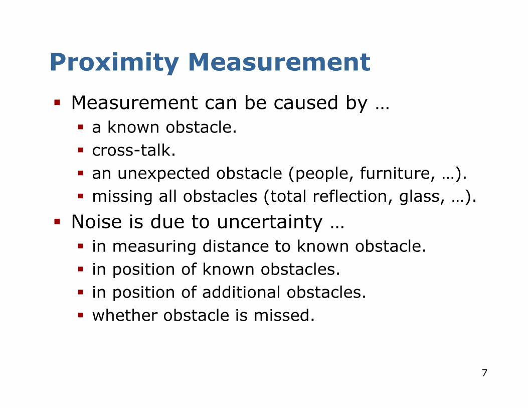
Proximity Measurement

� Measurement can be caused by …

� a known obstacle.

� cross-talk.

� an unexpected obstacle (people, furniture, …).

� missing all obstacles (total reflection, glass, …).

� Noise is due to uncertainty …

� in measuring distance to known obstacle.

� in position of known obstacles.

� in position of additional obstacles.

� whether obstacle is missed.

8

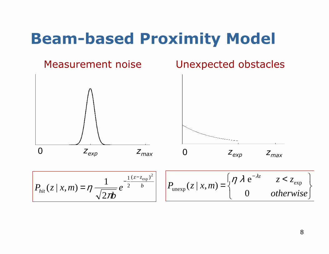
Beam-based Proximity Model

Measurement noise

zexp zmax0

b

zz

hit eb

mxzP

2exp)(

2

1

2

1),|(

−−

=π

η

<

=−

otherwise

zzmxzP

z

0

e),|( exp

unexp

λλη

Unexpected obstacles

zexp zmax0

9

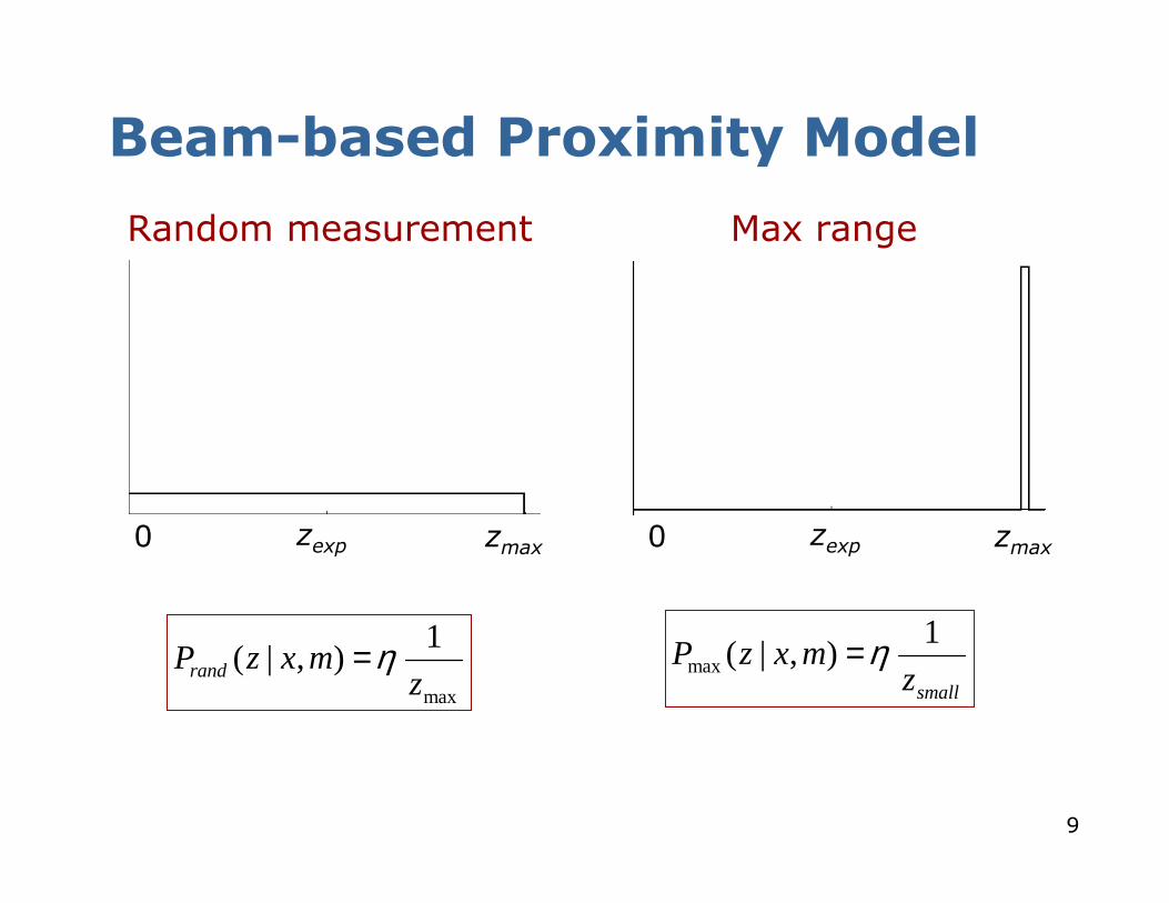
Beam-based Proximity Model

Random measurement Max range

max

1),|(

zmxzPrand η=

smallzmxzP

1),|(max η=

zexp zmax0zexp zmax0

10

Resulting Mixture Density

⋅

=

),|(

),|(

),|(

),|(

),|(

rand

max

unexp

hit

rand

max

unexp

hit

mxzP

mxzP

mxzP

mxzP

mxzP

T

αααα

How can we determine the model parameters?

11

Raw Sensor Data

Measured distances for expected distance of 300 cm.

Sonar Laser

12

Approximation

� Maximize log likelihood of the data

� Search space of n-1 parameters.� Hill climbing� Gradient descent� Genetic algorithms� …

� Deterministically compute the n-thparameter to satisfy normalization constraint.

)|( expzzP

13

Approximation Results

Sonar

Laser

300cm 400cm

14

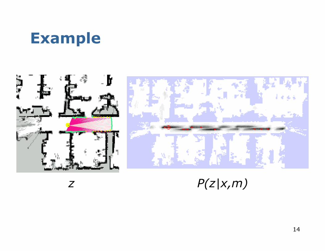
Example

z P(z|x,m)

15

Discrete Model of Proximity Sensors

� Instead of densities, consider discrete steps along the sensor beam.

� Consider dependencies between different cases.

Laser sensor Sonar sensor

16

Approximation Results

Laser

Sonar

17

"sonar-0"

0 10 20 30 40 50 60 70 010

2030

4050

6070

00.050.1

0.150.2

0.25

Influence of Angle to Obstacle

18

"sonar-1"

0 10 20 30 40 50 60 70 010

2030

4050

6070

00.050.1

0.150.2

0.250.3

Influence of Angle to Obstacle

19

"sonar-2"

0 10 20 30 40 50 60 70 010

2030

4050

6070

00.050.1

0.150.2

0.250.3

Influence of Angle to Obstacle

20

"sonar-3"

0 10 20 30 40 50 60 70 010

2030

4050

6070

00.050.1

0.150.2

0.25

Influence of Angle to Obstacle

21

Summary Beam-based Model

� Assumes independence between beams.

� Justification?

� Overconfident!

� Models physical causes for measurements.

� Mixture of densities for these causes.

� Assumes independence between causes. Problem?

� Implementation

� Learn parameters based on real data.

� Different models should be learned for different angles at which the sensor beam hits the obstacle.

� Determine expected distances by ray-tracing.

� Expected distances can be pre-processed.

22

Scan-based Model

� Beam-based model is …

� not smooth for small obstacles and at edges.

� not very efficient.

� Idea: Instead of following along the beam, just check the end point.

23

Scan-based Model

� Probability is a mixture of …

� a Gaussian distribution with mean at distance to closest obstacle,

� a uniform distribution for random measurements, and

� a small uniform distribution for max range measurements.

� Again, independence between different components is assumed.

24

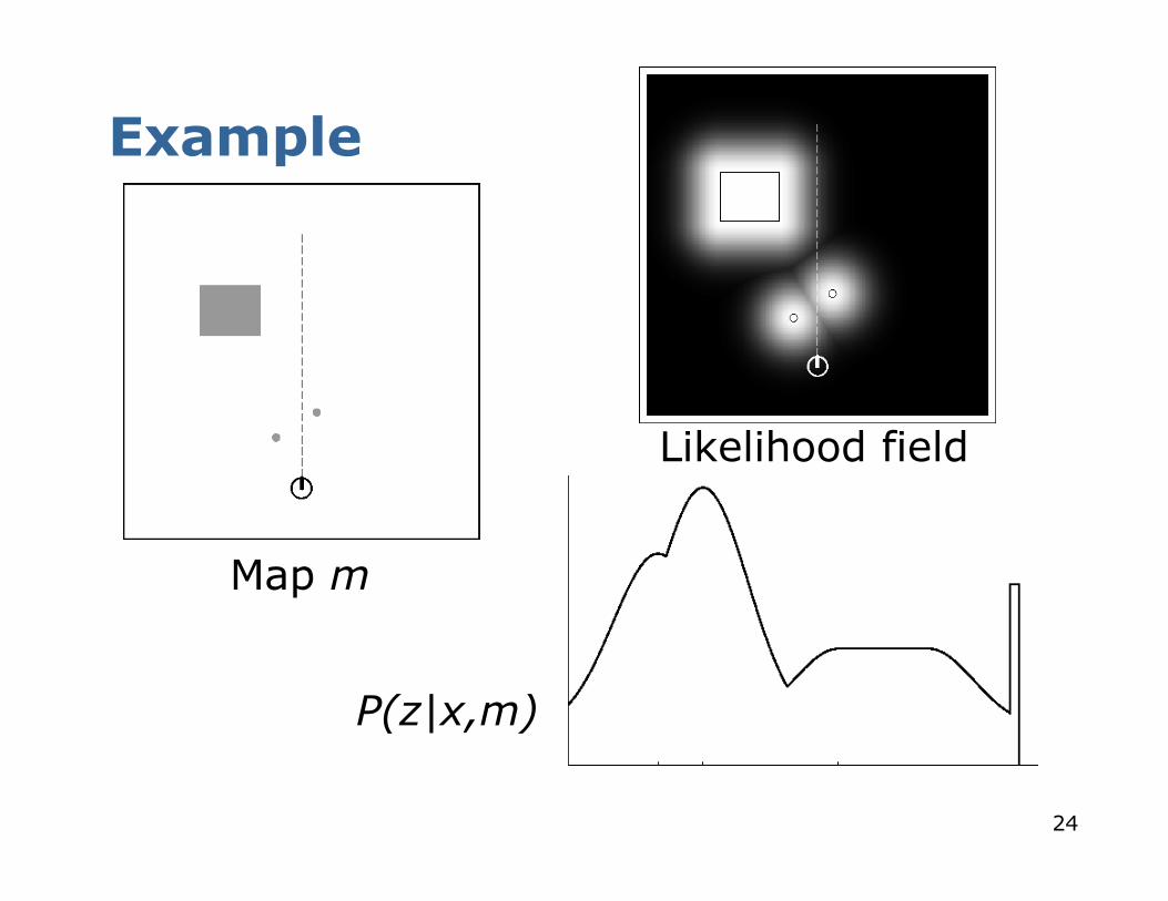
Example

P(z|x,m)

Map m

Likelihood field

25

San Jose Tech Museum

Occupancy grid map Likelihood field

26

Scan Matching

� Extract likelihood field from scan and use it to match different scan.

27

Scan Matching

� Extract likelihood field from first scan and use it to match second scan.

~0.01 sec

28

Properties of Scan-based Model

� Highly efficient, uses 2D tables only.

� Smooth w.r.t. to small changes in robot

position.

� Allows gradient descent, scan matching.

� Ignores physical properties of beams.

� Will it work for ultrasound sensors?

29

Additional Models of Proximity Sensors

� Map matching (sonar, laser): generate small, local maps from sensor data and match local maps against global model.

� Scan matching (laser): map is represented by scan endpoints, match scan into this map.

� Features (sonar, laser, vision): Extract features such as doors, hallways from sensor data.

30

Landmarks

� Active beacons (e.g., radio, GPS)

� Passive (e.g., visual, retro-reflective)

� Standard approach is triangulation

� Sensor provides

� distance, or

� bearing, or

� distance and bearing.

31

Distance and Bearing

32

Probabilistic Model

1. Algorithm landmark_detection_model(z,x,m):

2.

3.

4.

5. Return

22 ))(())((ˆ yimximd yx −+−=

),ˆprob(),ˆprob(det αεααε −⋅−= dddp

θα ,,,,, yxxdiz ==

θ−−−= ))(,)(atan2(ˆ ximyima xy

),|(uniformfpdetdet mxzPzpz +

33

Distributions

34

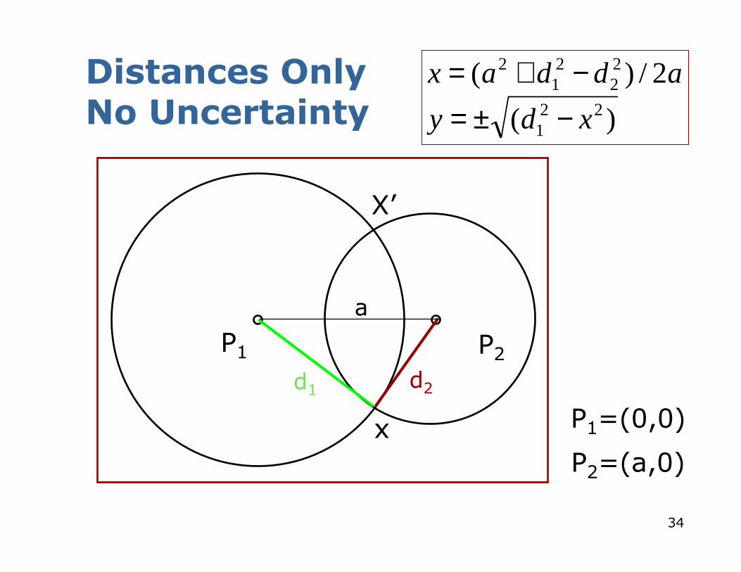
Distances OnlyNo Uncertainty

P1 P2

d1 d2

x

X’

a

)(

2/)(22

1

22

21

2

xdy

addax

−±=−+=

P1=(0,0)

P2=(a,0)

35

P1

P2

D1

z1

z2α

P3

D2

βz3

D3

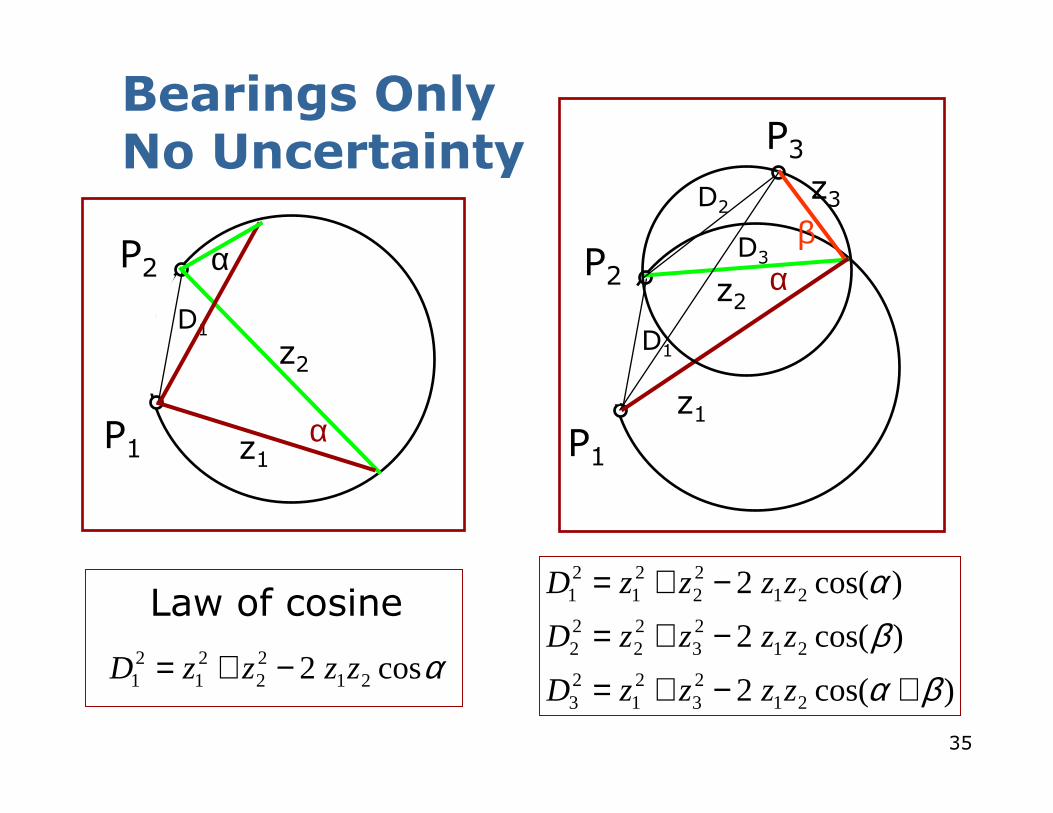
Bearings OnlyNo Uncertainty

P1

P2

D1

z1

z2

α

α

αcos2 2122

21

21 zzzzD −+=

)cos(2

)cos(2

)cos(2

2123

21

23

2123

22

22

2122

21

21

βαβα

+−+=

−+=

−+=

zzzzD

zzzzD

zzzzDLaw of cosine

36

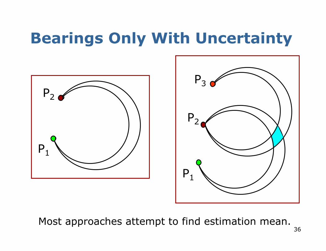
Bearings Only With Uncertainty

P1

P2

P3

P1

P2

Most approaches attempt to find estimation mean.

37

Summary of Sensor Models

� Explicitly modeling uncertainty in sensing is key to robustness.

� In many cases, good models can be found by the following approach:

1. Determine parametric model of noise free measurement.

2. Analyze sources of noise.

3. Add adequate noise to parameters (eventually mix in densities for noise).

4. Learn (and verify) parameters by fitting model to data.

5. Likelihood of measurement is given by “probabilistically comparing” the actual with the expected measurement.

� This holds for motion models as well.

� It is extremely important to be aware of the underlying assumptions!