introduction to markov state model (msm): part i
TRANSCRIPT

Introduction to Markov State Model (MSM): Part I

Molecular Dynamics SimulationStructure Force field
Conditions
MDNewton’s Law
TrajectoriesSeries of structuresat specified times

Timescale gapg p
Markov State Model (MSMs): a kinetic network model can enhance sampling and bridge the gap between experiments and simulationssampling and bridge the gap between experiments and simulations.
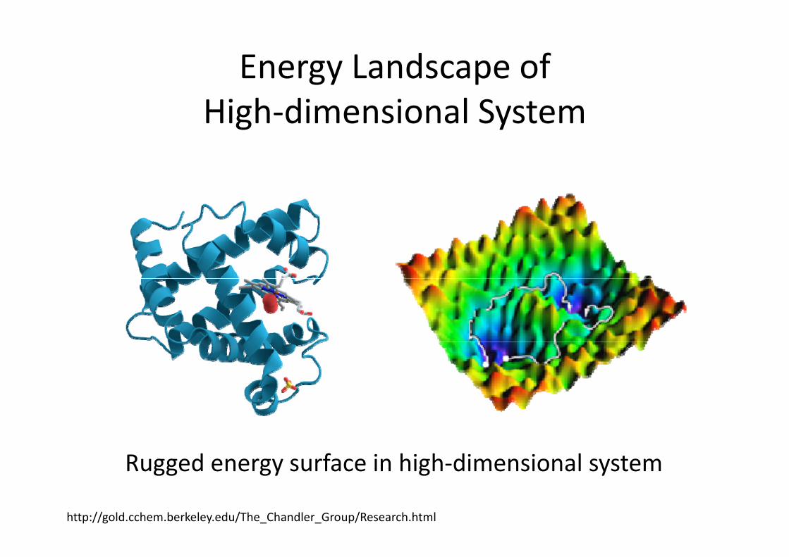
Energy Landscape ofHigh‐dimensional System
Rugged energy surface in high‐dimensional system
http://gold.cchem.berkeley.edu/The_Chandler_Group/Research.html
Rugged energy surface in high dimensional system

Sampling issuep g
~370,000 atoms370,000 atoms

Sampling issuep g
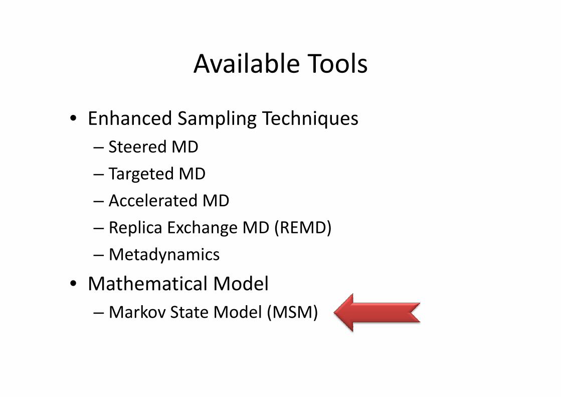
Available ToolsAvailable Tools
• Enhanced Sampling Techniques– Steered MD– Targeted MDAccelerated MD– Accelerated MD
– Replica Exchange MD (REMD)– Metadynamics
• Mathematical ModelMathematical Model– Markov State Model (MSM)

Building the Markov State Models (MSMs)Building the Markov State Models (MSMs)
Raw data Microstates MacrostatesRaw data (conformations)
Microstates (geometry clustering)
Macrostates (metastable states)
Local equilibrium
Methods 2009, 49, 197–201
Local equilibrium within discrete state

Building the Markov State Models (MSMs)
• Geometric clustering for microstatesg• (Assumes similar kinetic behavior within state)
• Drawing the implied timescale plot• (Determines the lag time at which the system can be• (Determines the lag time at which the system can be approximated as a Markovian model)
• (Choose the number of macrostate)
L mping the microstates into macrostates• Lumping the microstates into macrostates• (Maintaining similar kinetic behaviour within state)

Geometric clustering for microstatesGeometric clustering for microstates

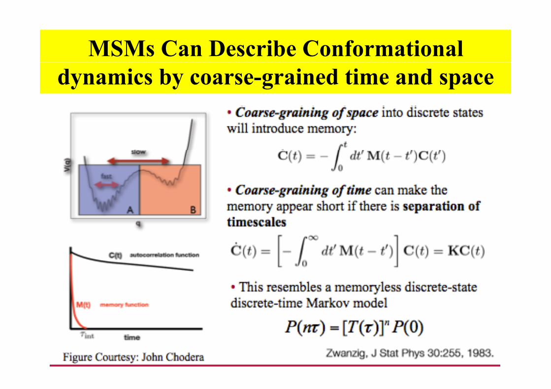
MSM Can Describe Conformational dynamics by coarse-grained time and space
Coarse-graining of space intod ll ddiscrete states will introducememory.
Coarse-graining of time canmake the memory appear shortif there is separation oftimescales.
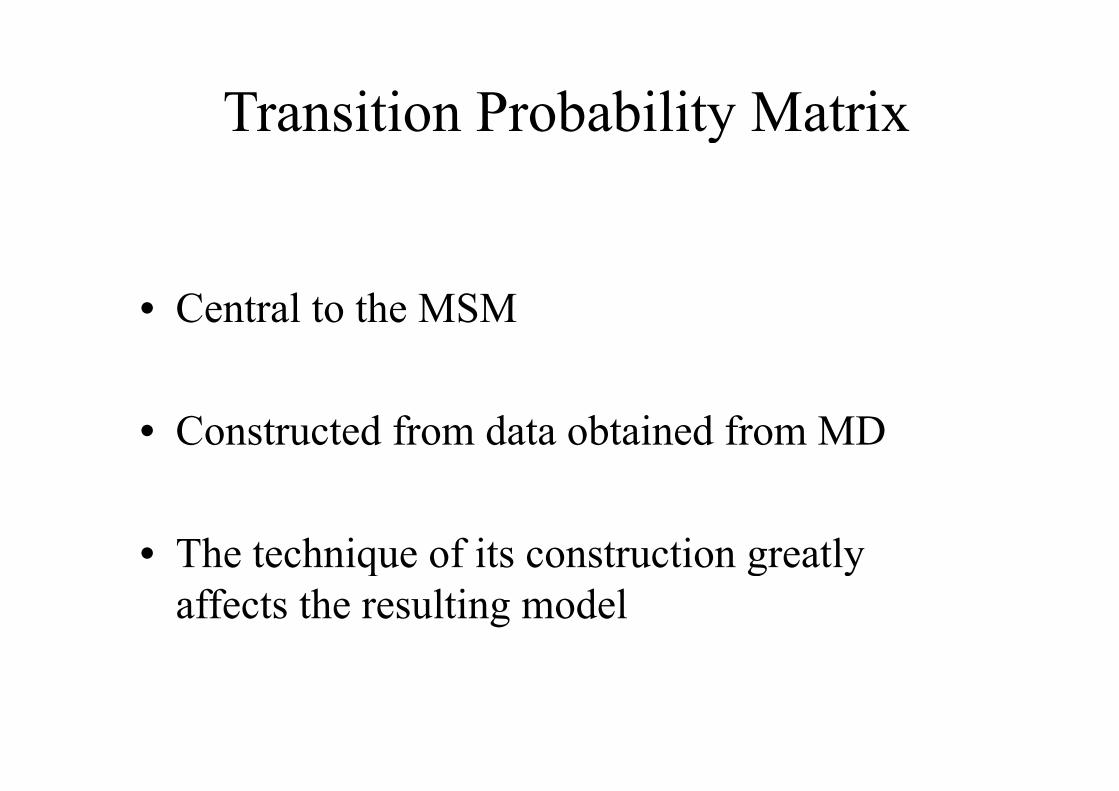
Transition Probability MatrixTransition Probability Matrix
• Central to the MSM• Central to the MSM
• Constructed from data obtained from MD
• The technique of its construction greatly q g yaffects the resulting model
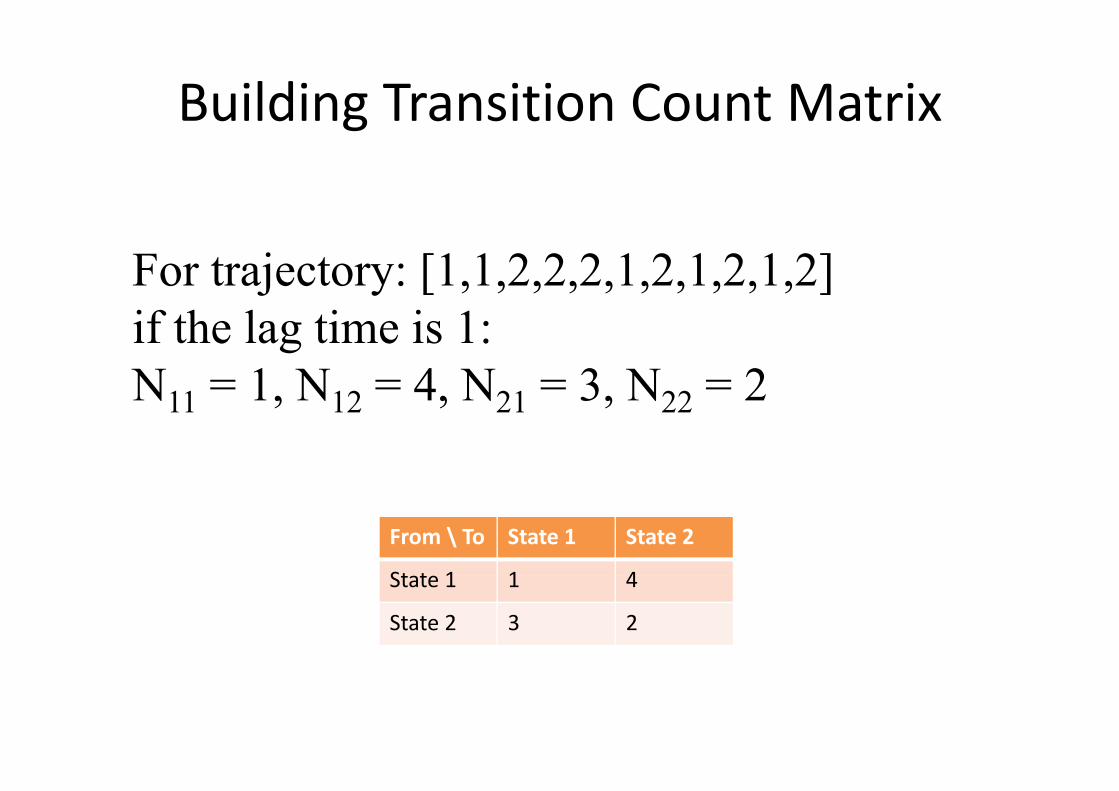
Building Transition Count Matrixg
For trajectory: [1,1,2,2,2,1,2,1,2,1,2] if the lag time is 1:N11 = 1 N12 = 4 N21 = 3 N22 = 2N11 1, N12 4, N21 3, N22 2
From \ To State 1 State 2
St t 1 1 4State 1 1 4
State 2 3 2

Detailed BalanceDetailed Balance
• At equilibrium, all the elementary transitions should also be at equilibrium (Detailed q (Balance) Equally likely at
both directions
p1p1
p3
p2
p3
p2

Detailed BalanceDetailed Balance
• Detailed balance implies having a transition from state i to j should be equally likely as j q y yhaving a transition from state j to i
• Because the actual number of transition is• Because the actual number of transition is determined by the product of population and
b b l htransition probability, we have:p1p1
=p2

Fulfilling Detailed BalanceFulfilling Detailed BalanceFrom \ To State 1 State 2
• Symmetrizing TCM by:
Τ
State 1 1 4
State 2 3 2
N symm =N + N Τ
2 From \ To State 1 State 2
• Generate TPM by:
2 \
State 1 1 3.5
State 2 3.5 2Generate TPM by:
Nsymm
Pij = N
ij
(Nsymm )∑From \ To State 1 State 2
State 1 0.222 0.778(N
ij)∑ State 2 0.636 0.364

Building the MSMBuilding the MSM
( )N τ( )( )
( )ij
ijij
j
NT
Nτ
ττ
=∑
j
T i i P b bili M iTransition Probability Matrix
( ) [ ( )] (0)nP n T Pτ τ=
Where P(nτ) is a vector of state populations at time nτWhere P(nτ) is a vector of state populations at time nτ.
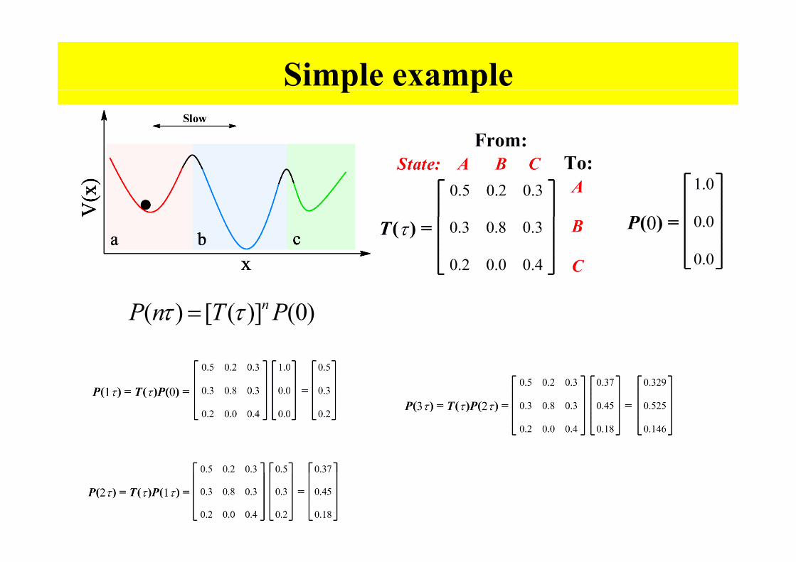
Simple examplep p
( ) [ ( )] (0)nP n T Pτ τ=
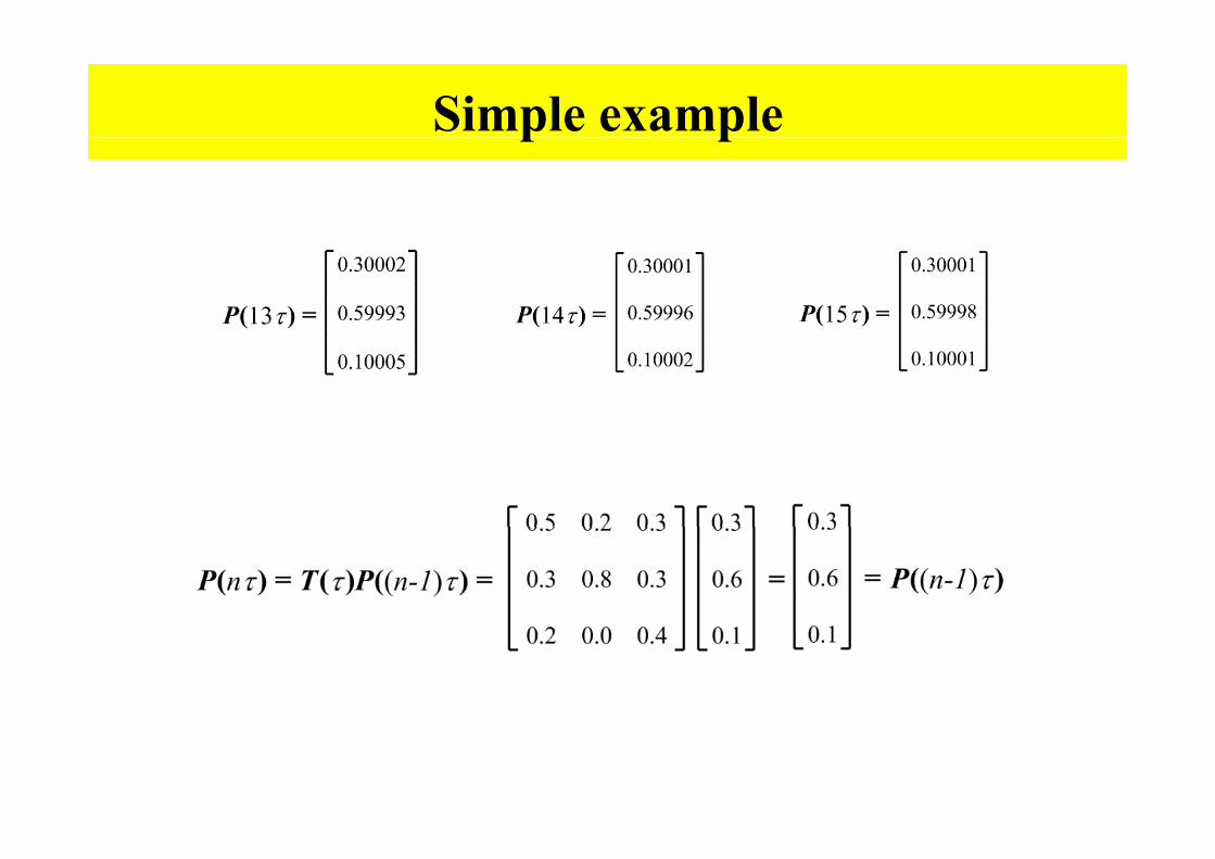
Simple examplep p

Building the MSMg
n=100
J. Chem. Phys. 2011, 134, 174105

Building the MSMBuilding the MSM
( )T τ λΦ = Φ( ) i i iT τ λΦ = Φ
λi is an eigenvalue corresponding to eigenvector Φi
1( ) n
i i ii
P n cτ λ=
= Φ∑J. Chem. Phys. 2011, 134, 174105

Implied timescalesImplied timescales
Validation of MSM: #1
ln ( )kk
ττμ τ
= −( )kμ
Lag time τ (ns)
J. Chem. Phys. 2011, 134, 174105

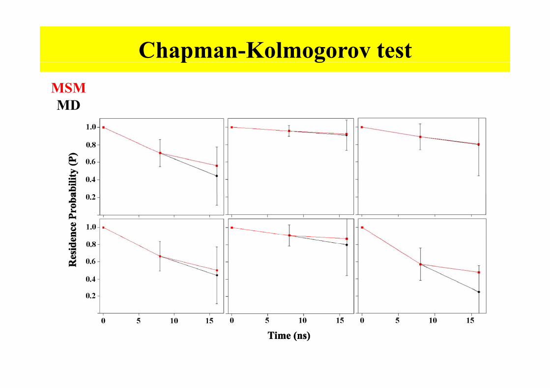
Validation of MSM: #2Validation of MSM: #2
Chapman-Kolmogorov TestChapman-Kolmogorov Test
( ) [ ( )]nMD MSMP n Pτ τ=
To check if A MarkovianTo check if A Markovian model can “well-represent” MDrepresent MD.
J. Chem. Phys. 2011, 134, 174105

What can we know from an MSM?What can we know from an MSM?
• Thermodynamic information– Equilibrium populationsq p p
f• Kinetic information– Mean first passage time– Dominant Pathways (pathways with major flux)
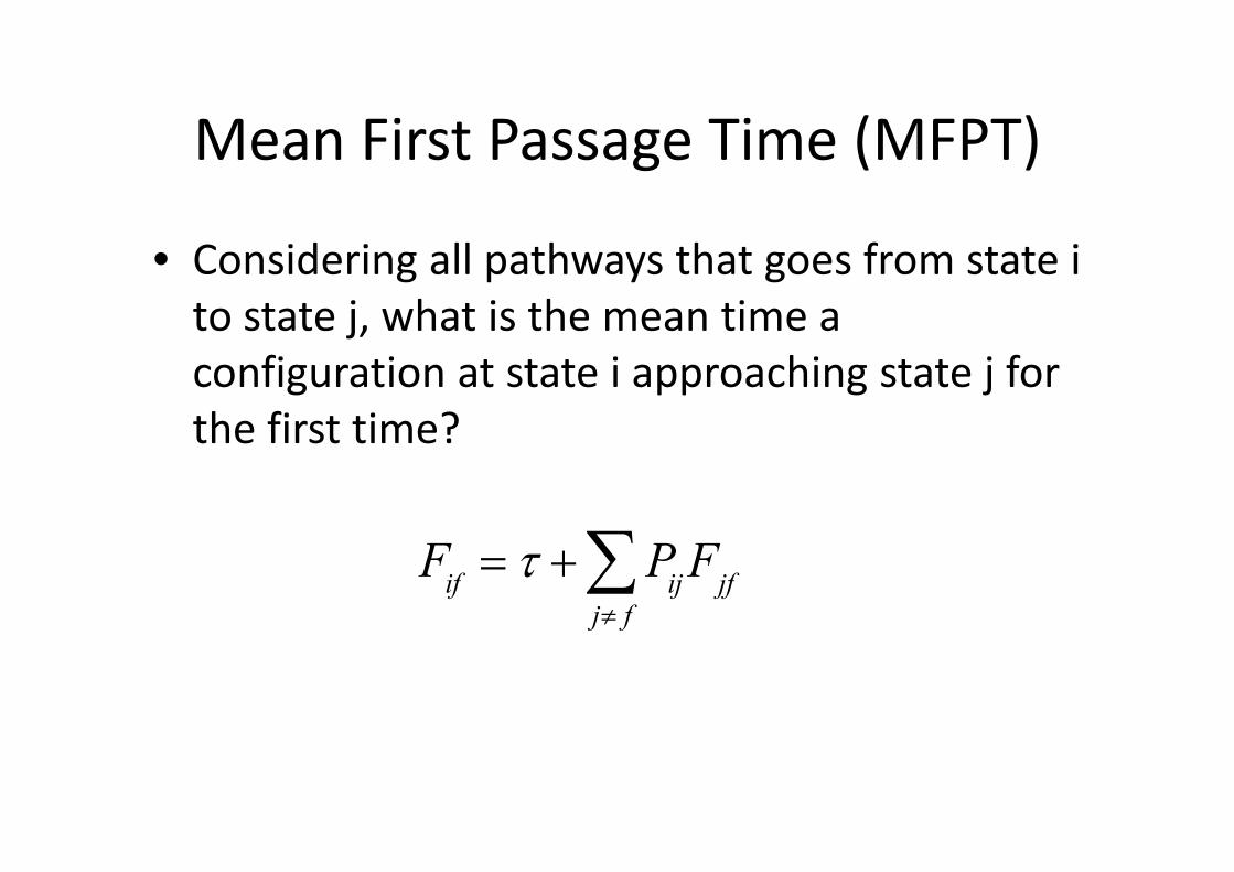
Mean First Passage Time (MFPT)Mean First Passage Time (MFPT)
• Considering all pathways that goes from state i to state j, what is the mean time a jconfiguration at state i approaching state j for the first time?the first time?
∑Fif = τ + Pijj≠ f∑ Fjf

MFPT for 3 state ModelMFPT for 3‐state Model
Fif = τ + Pijj≠ f∑ Fjfj≠ f

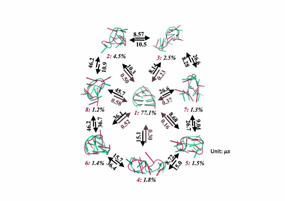
Mean first passage timeMean first passage time
MFPT: the mean time it takes to reach a given metastable state ff th fi t ti h t ti f th t t ifor the first time when starting from another state i.

Transition path theoryTransition path theory

Introduction to MSM: Part II


Example systemExample system
Constant temperature MD psimulations (400K).
Amber96 force field.
100 500-ps MD simulations with conformation stored at 1ps.
Total conformation: 50,000

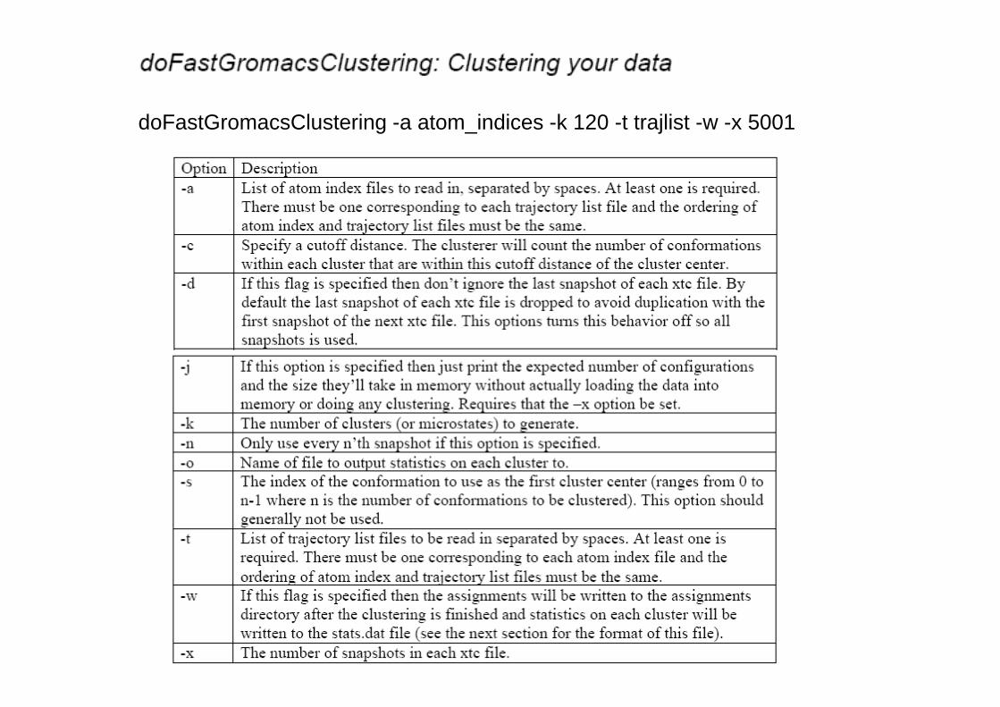
doFastGromacsClustering -a atom_indices -k 120 -t trajlist -w -x 5001

Check your stats.dat file
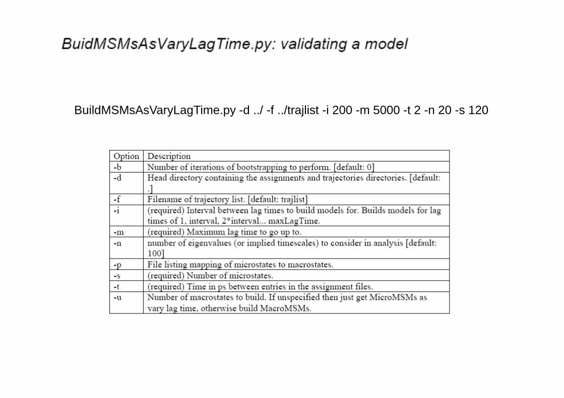
BuildMSMsAsVaryLagTime py d / f /trajlist i 200 m 5000 t 2 n 20 s 120BuildMSMsAsVaryLagTime.py -d ../ -f ../trajlist -i 200 -m 5000 -t 2 -n 20 -s 120


BuildMacroMSM.py -d ../ -f ../trajlist -l 1 -m 3 -s 300 -t 1 -n 0 -x
WriteMacroAssignments.py -d ../ -f ../trajlist -m mapMicroToMacro.dat

GetMicroCenters.py -d ./ -f trajlist -t ../file00001.pdb -x ./index.ndx
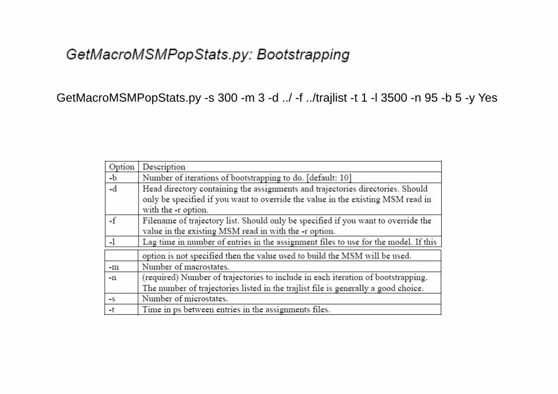
GetMacroMSMPopStats.py -s 300 -m 3 -d ../ -f ../trajlist -t 1 -l 3500 -n 95 -b 5 -y Yes
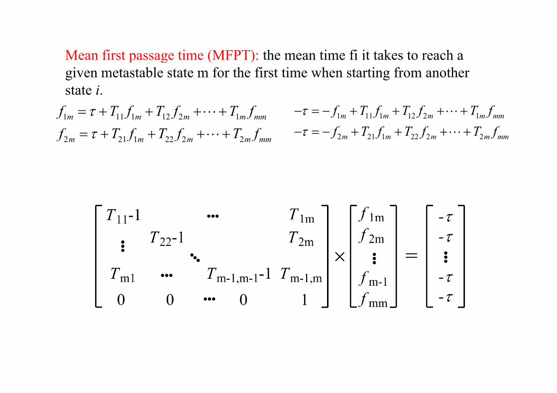
Mean first passage time (MFPT): the mean time fi it takes to reach a p g ( )given metastable state m for the first time when starting from another state i.
f T f T f T f f T f T f T f1 11 1 12 2 1
2 21 1 22 2 2
m m m m mm
m m m m mm
f T f T f T ff T f T f T f
ττ
= + + + ⋅⋅⋅ += + + + ⋅⋅⋅ +
1 11 1 12 2 1
2 21 1 22 2 2
m m m m mm
m m m m mm
f T f T f T ff T f T f T f
ττ− = − + + + ⋅⋅⋅ +
− = − + + + ⋅⋅⋅ +

MFPT.py -f ../trajlist -s 300 -t 1 -l 3500 -u 3 -d ../
O iOptions:-h, --help show this help message and exit-d HEADDIR, --head_dir=HEADDIR
Head direectory containing the assignments andtrajectories directories. [default: .]j [ ]
-f TRAJLISTFN, --traj_list=TRAJLISTFNFilename of trajectory list. [default: trajlist]
-p MAPMICROTOMACROFN, --mapMicroToMacroFn=MAPMICROTOMACROFNFile listing mapping of micro states to macro states.
-s NMICROSTATES --numMicroStates=NMICROSTATES-s NMICROSTATES, --numMicroStates=NMICROSTATES(required) Number of microstaes.
-t DT, --time_step=DT(required) Time in ps between entries in theassignment files.
k SKIPMACROZERO Ski M Z SKIPMACROZERO-k SKIPMACROZERO, --Skip_Macro_Zero=SKIPMACROZEROAre we skipping Macrostate 0 when computing Macrostateimplied timescale plots? Only useful when interfacingwith Mapper, default should be 0
-l LAGT, --Lag_time=LAGTg_(required) Lag time in step number.
-u NUMMACRO, --num_macro=NUMMACRONumber of macrostates in the system.
-a COMPUTEALL, --Compute_ALL=COMPUTEALLcompute all the MFPT or only a subset of the statescompute all the MFPT or only a subset of the states
-y GETRIDOF, --yes=GETRIDOFif you want to get rid of the recrossing

Introduction to MSM: Part III

Structure of RNA polymerase IIp y
Wang, D et al. Cell 2006, 127, 941-954
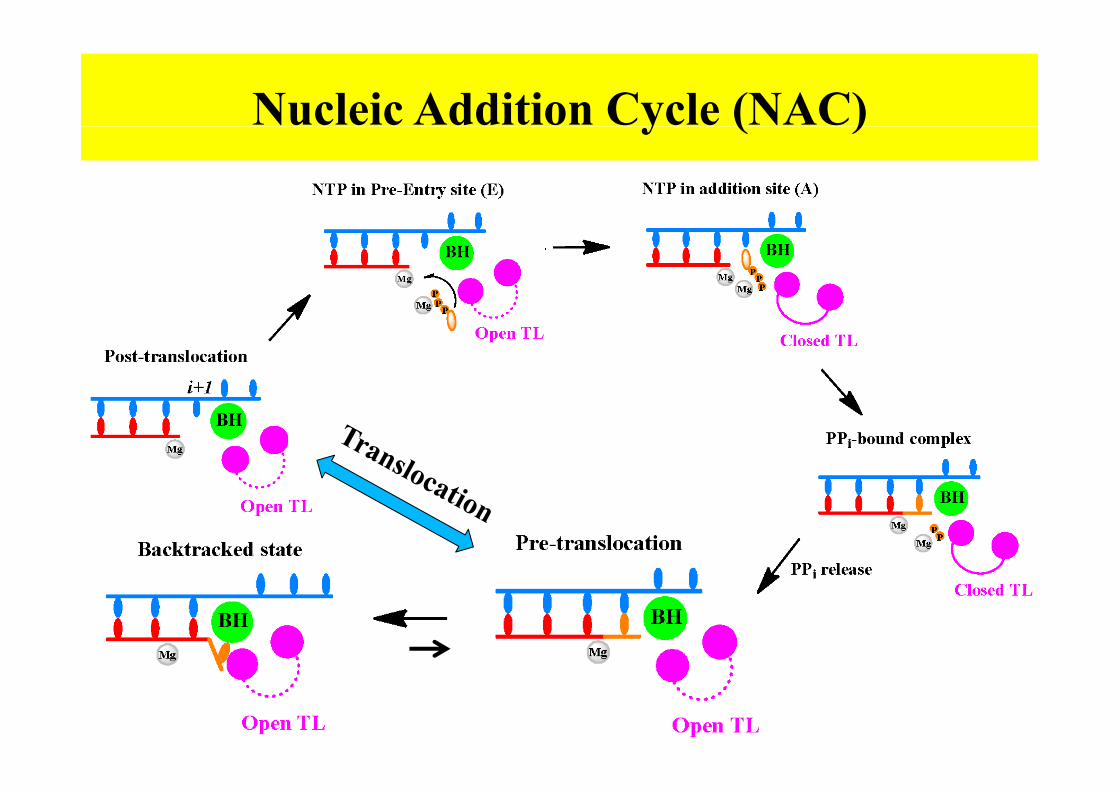
Nucleic Addition Cycle (NAC)y ( )

PPi release mechanismi e e se ec s

The problems we are interestedp
1 H d h PP i l l h d h l f l II ?1. How does the PP ion release along the secondary channel of pol II ?
2. What is the correlations between the PPi release and theconformational changes of trigger loop? And translocation?
3. What is the difference of the PPi release between the pol II andff f pbacterial RNA polymerase?

Simulation methodologygy

PPi-bound pol II complexp p
B d GTP b d l II l (2E2H)Based on GTP-bound pol II complex (2E2H) Da, LT et al, J. Am. Chem. Soc., 134, 2399, (2012)

System setupy p
1 S i 3 0 0001. System size ~370,000 atoms.Protein (> 3000 residues), water, DNA, RNA, ions, etc.
2. Built the MSM based on 122 trajectories (6ns each).j ( )
3. Traced the PPi release dynamics around 1 5μsaround 1.5μs

PPi release adopts a hopping modep pp g
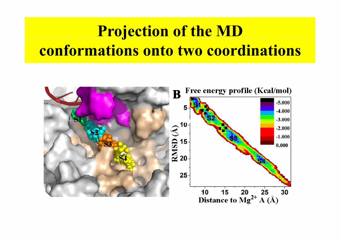
Projection of the MD jconformations onto two coordinations
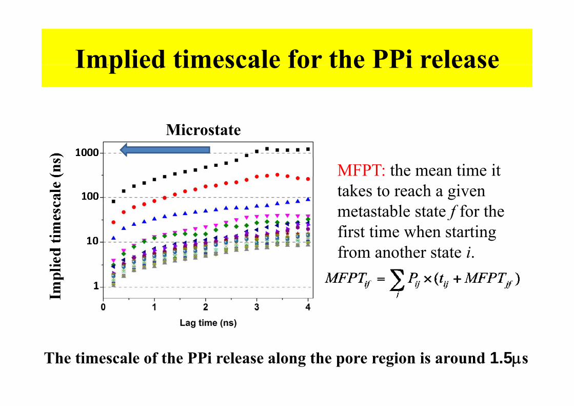
Implied timescale for micro and macroImplied timescale for the PPi releasepImplied timescale for the PPi release
Microstate
MFPT: the mean time it takes to reach a given metastable state f for the first time when starting f th t t ifrom another state i.
The timescale of the PPi release along the pore region is around 1.5μs

Translocation mechanisms oc o ec s

Simulation methodologygy
Silva, DA. et al, Proc. Nat. Acad. Sci. U.S.A., (Accepted)

Four metastable states

Validation of the MSM

Thermodynamic and kinetic property y p p y

谢谢!谢谢

Two proposed backtracking modelsTwo proposed backtracking models
Pre-, frayed and backtracked models
Cli b l ith
Conformations along low energy pathways
Climber algorithm
energy pathways
Unbiased MDMD simulations
MSM constructionconstruction
Backtracking mechanism

Initial low-energy backtracking pathwaysInitial low energy backtracking pathways
Pre-, frayed and backtracked models
Cli b l ith
Conformations along low energy pathways
Climber algorithm
energy pathways
Unbiased MDMD simulations
MSM constructionconstruction
Backtracking mechanism
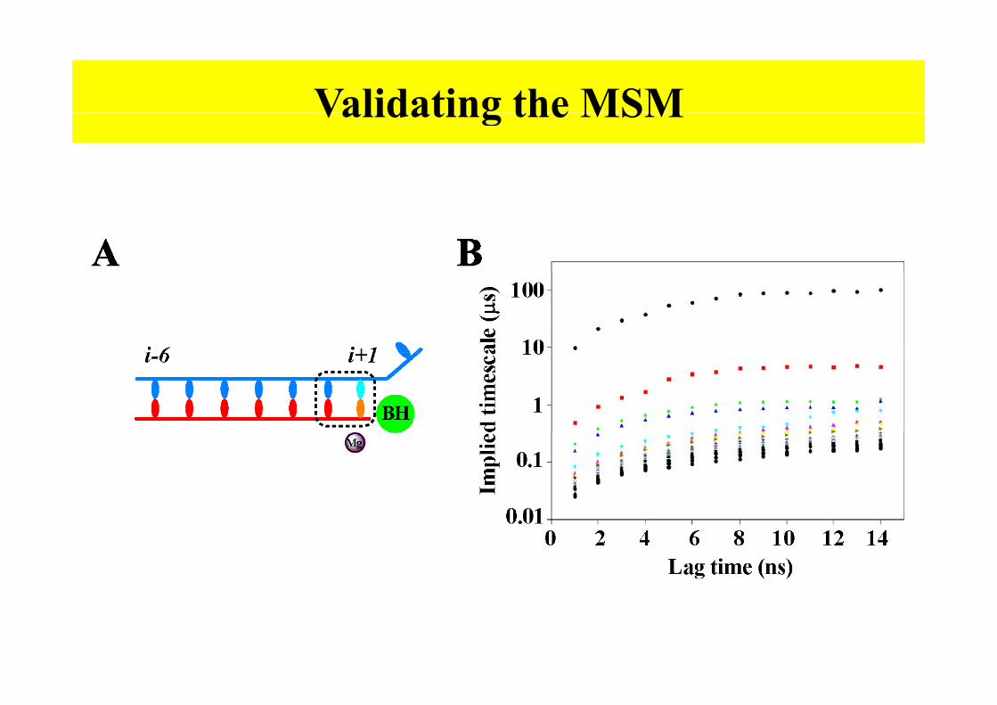
Validating the MSMValidating the MSM
Chapman-Kolmogorov testp gMSMMDMD

Four metastable states identified by MSMFour metastable states identified by MSM

Backtracking preference
Potential of Mean Force (kcal/mol)
g p
s (Å
)uc
leot
ides
S4
o D
NA
nu
S3
MSD
of t
wo
S2TS
RM S1 S2TS
RMSD of two RNA 3′-end nucleotides (Å)

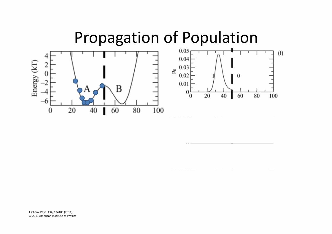
A Two well PotentialA Two‐well Potential
J. Chem. Phys. 134, 174105 (2011)© 2011 American Institute of Physics

Propagation of PopulationPropagation of Population
J. Chem. Phys. 134, 174105 (2011)© 2011 American Institute of Physics

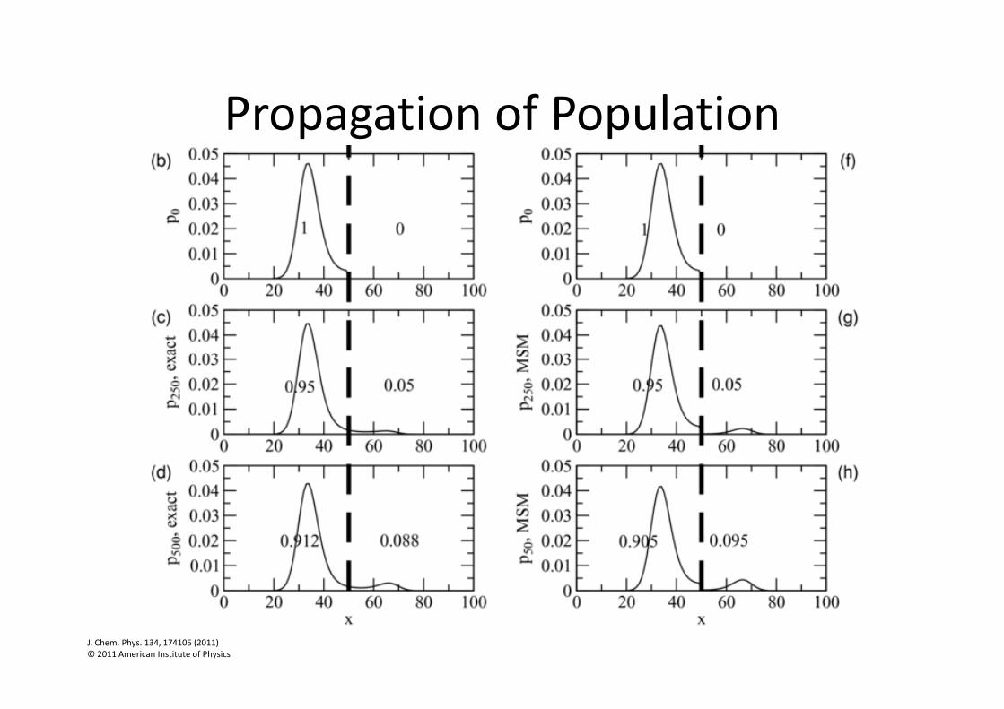
Propagation of PopulationPropagation of Population
J. Chem. Phys. 134, 174105 (2011)© 2011 American Institute of Physics

Propagation of PopulationPropagation of Population
J. Chem. Phys. 134, 174105 (2011)© 2011 American Institute of Physics
Propagation of PopulationPropagation of Population
J. Chem. Phys. 134, 174105 (2011)© 2011 American Institute of Physics

Propagation of PopulationPropagation of Population
J. Chem. Phys. 134, 174105 (2011)© 2011 American Institute of Physics

Propagation of PopulationPropagation of Population
J. Chem. Phys. 134, 174105 (2011)© 2011 American Institute of Physics
Propagation of PopulationPropagation of Population
J. Chem. Phys. 134, 174105 (2011)© 2011 American Institute of Physics
“Memory” vs Markovian AssumptionMemory vs Markovian Assumption
• Discretization introduces memory
• A Markov model is a “memoryless model” (or l h fi i f )only have a finite amount of memory)
• The challenge of using MSM to analyze MD d t i th f i i i i th ff t fdata is therefore minimizing the effect of “memory”

Problems with Very Long Lag TimeProblems with Very Long Lag Time

What else can we do?What else can we do?
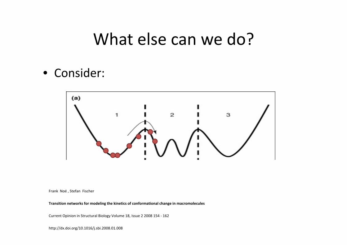
• Consider:
Frank Noé , Stefan Fischer
Transition networks for modeling the kinetics of conformational change in macromolecules
Current Opinion in Structural Biology Volume 18, Issue 2 2008 154 ‐ 162
http://dx.doi.org/10.1016/j.sbi.2008.01.008
What else can we do?What else can we do?
• Consider:
Frank Noé , Stefan Fischer
Transition networks for modeling the kinetics of conformational change in macromolecules
Current Opinion in Structural Biology Volume 18, Issue 2 2008 154 ‐ 162
http://dx.doi.org/10.1016/j.sbi.2008.01.008

Difference Between Real and Propagated Dynamics

What else can we do?What else can we do?
• Discretize the configuration space such that:
– There is no internal barrier within all the states
– In other words, always cut the very top of each b ibarrier

Choose the Markovian Lag Time Under Our Commonly Used Frameworkh i h i h h h i li d• Choosing the time such that the implied
timescale plot of the slow modes plateaued
• The flattened implied timescale implies theThe flattened implied timescale implies the populations are roughly “equilibrated” in such transition modestransition modes
• Validation via Chapman‐Kolmogorov test is still necessary

Challenge QuestionChallenge Question
• Rank of the following discretization on how well each model represents the original p genergy landscape?
1 (best) 23 4 (worst)
J. Chem. Phys. 134, 174105 (2011)© 2011 American Institute of Physics
J. Chem. Phys. 134, 174105 (2011)© 2011 American Institute of Physics
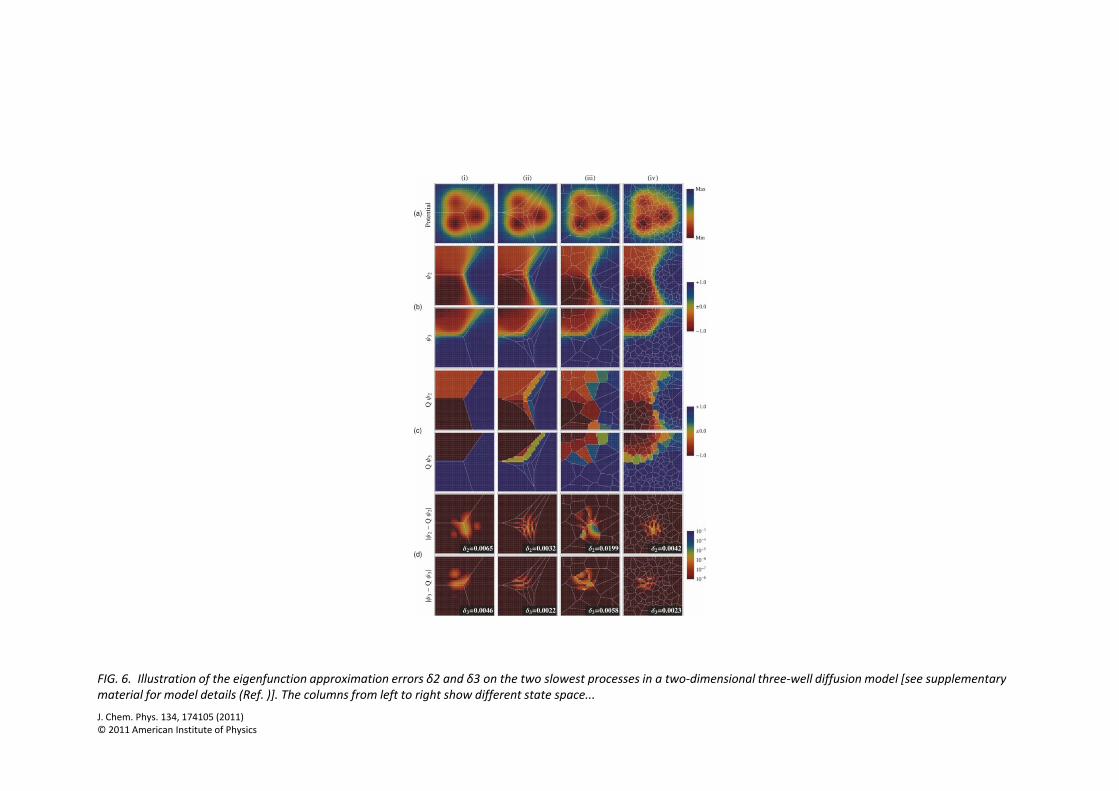
FIG. 6. Illustration of the eigenfunction approximation errors δ2 and δ3 on the two slowest processes in a two‐dimensional three‐well diffusion model [see supplementary material for model details (Ref. )]. The columns from left to right show different state space...

ObservationsObservations
• The model with the most number of state is not the best
• The model with the least number of state is not the worstnot the worst
• The model with highest metastability is not the best
J. Chem. Phys. 134, 174105 (2011)© 2011 American Institute of Physics
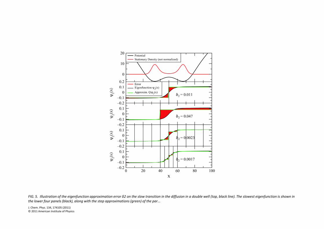
FIG. 5. Illustration of the eigenfunction approximation error δ2 on the slow transition in the diffusion in a double well (top, black line). The slowest eigenfunction is shown in the lower four panels (black), along with the step approximations (green) of the par...

Compromise Between FactorsCompromise Between Factors
Temporal Resolution
Statistical Significance
Spatial Resolution

Flux AnalysisFlux Analysis
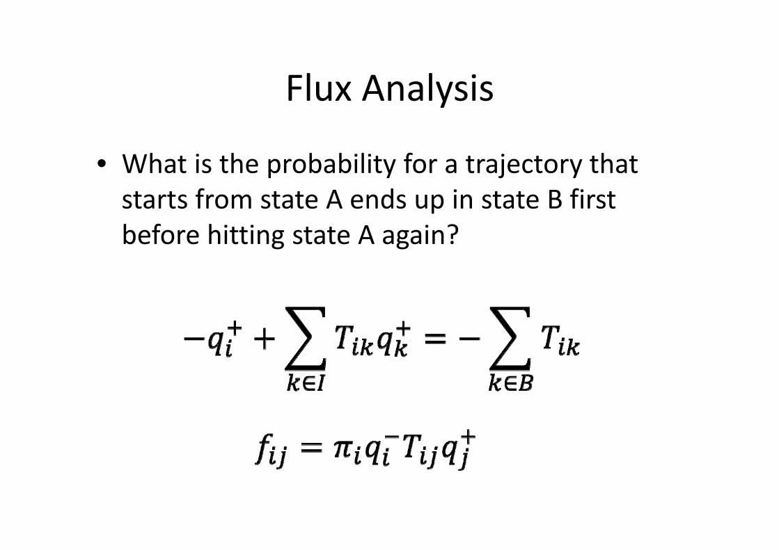
• What is the probability for a trajectory that starts from state A ends up in state B first pbefore hitting state A again?
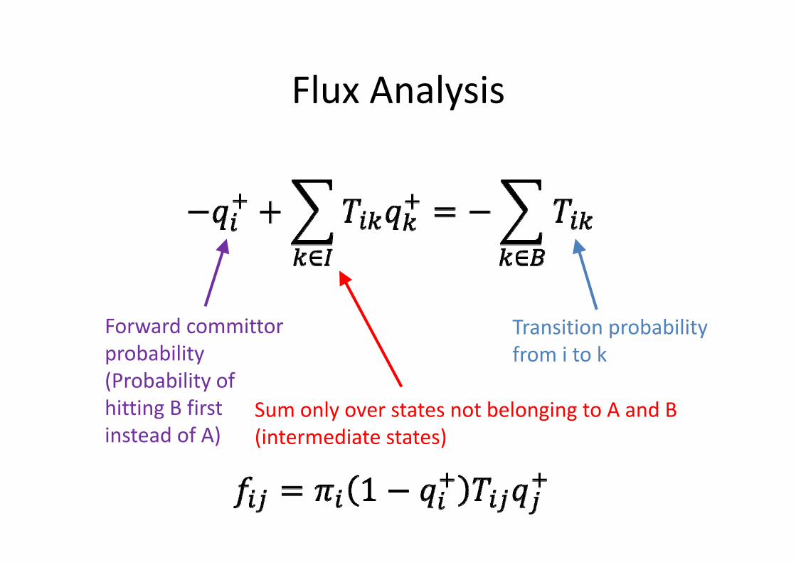
Flux AnalysisFlux Analysis
Transition probability Forward committor b b l
Sum only over states not belonging to A and B
from i to kprobability (Probability of hitting B first Sum only over states not belonging to A and B
(intermediate states)hitting B first instead of A)

Approximating the Energy LandscapeApproximating the Energy Landscape
Minima on energy landscape represented asMinima on energy landscape represented as nodes in a kinetic scheme
F. Noe, S. Fischer, Transition networks for modeling the kinetics of conformational change in macromolecules. Current opinion in structural biology 18, 154 (Apr, 2008).http://upload.wikimedia.org/wikipedia/commons/f/fc/Kinetic_scheme.jpg
MSMs Can Describe Conformational dynamics by coarse-grained time and space
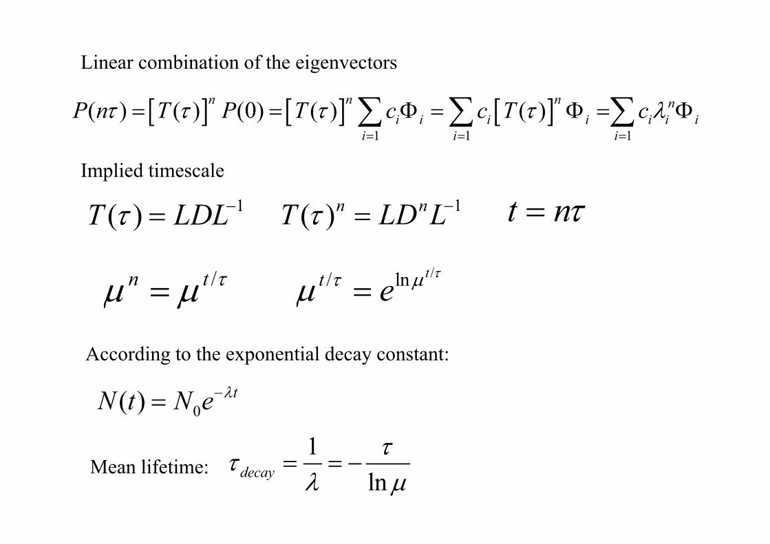
Linear combination of the eigenvectors
[ ] [ ] [ ]1 1 1
( ) ( ) (0) ( ) ( )n n n ni i i i i i i
i i i
P n T P T c c T cτ τ τ τ λ= = =
= = Φ = Φ = Φ∑ ∑ ∑
1( )n nT LD L− t nτ=1( )T LDL−
Implied timescale
1( )n nT LD Lτ = t nτ=
/ /t τ
1( )T LDLτ =
/n t τμ μ=// ln tt eττ μμ =
According to the exponential decay constant:
( ) tN t N λ−0( ) tN t N e λ=
1 τlndecayτ
λ μ= = −Mean lifetime:

Mean first passage time (MFPT): the mean time fi it takes to reach a p g ( )given metastable state m for the first time when starting from another state i.
f T f T f T f f T f T f T f1 11 1 12 2 1
2 21 1 22 2 2
m m m m mm
m m m m mm
f T f T f T ff T f T f T f
ττ
= + + + ⋅⋅⋅ += + + + ⋅⋅⋅ +
1 11 1 12 2 1
2 21 1 22 2 2
m m m m mm
m m m m mm
f T f T f T ff T f T f T f
ττ− = − + + + ⋅⋅⋅ +
− = − + + + ⋅⋅⋅ +

Chapman Kolmogorov EquationChapman‐Kolmogorov Equation
• For a discrete‐state time‐homogenous model that assumes Markovian property, we have p p ythe Chapman‐Kolmogorov Equation:
P(t + s) = P(t)P(s)• Thus, for a Markovian model that well‐represents the original system we shouldrepresents the original system, we should have:
well‐represents Markovian

Chapman Kolmogorov TestChapman‐Kolmogorov Test
• Chapman‐Kolmogorov Test
A “Markovian” –holds within the margin of error model that “well‐
represents” MD
• Any tests that follows such procedure can be id d “Ch K l t t”considered as “Chapman‐Kolmogorov test”

A Commonly Used ImplementationA Commonly Used Implementation
(TPM of the MSM)n
If a complete dataset is used, the equality should hold strictly at n = 0 and n = 1

Testing the DatasetTesting the Dataset
And so is other (k‐1) equalities

Accounting for Uncertaintiesin Simulation
• One‐sigma Standard Error
• BootstrappingBootstrapping
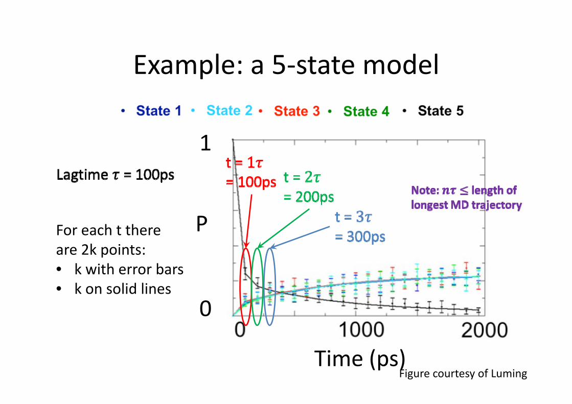
Example: a 5 state modelExample: a 5‐state model
1
PFor each t there are 2k points:are 2k points:• k with error bars • k on solid lines
0k on solid lines
Time (ps)Figure courtesy of Luming
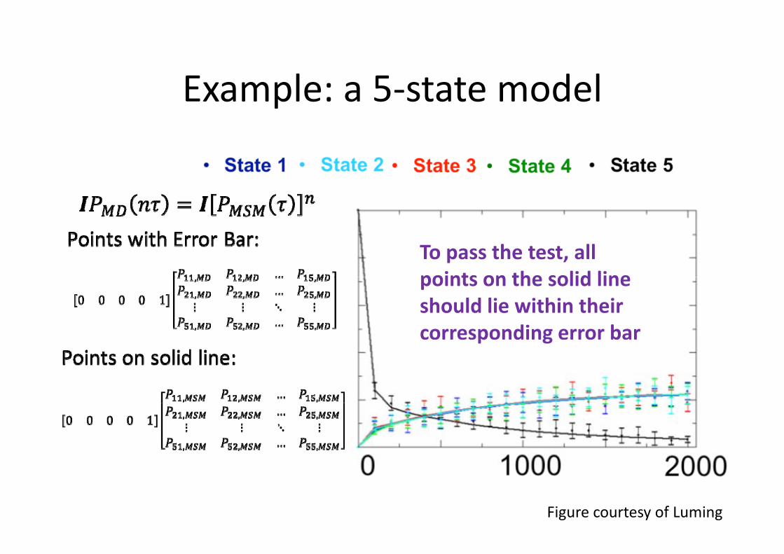
Example: a 5 state modelExample: a 5‐state model
To pass the test, all points on the solid linepoints on the solid line should lie within their corresponding error barp g
Figure courtesy of Luming

Pass or Fail?Pass or Fail?
Figure courtesy of Luming

Example: a 5 state modelExample: a 5‐state model
I NImportant Note:This graph only represent one of the five rows of theone of the five rows of the matrix, other four rows also need to be tested
Figure courtesy of Luming
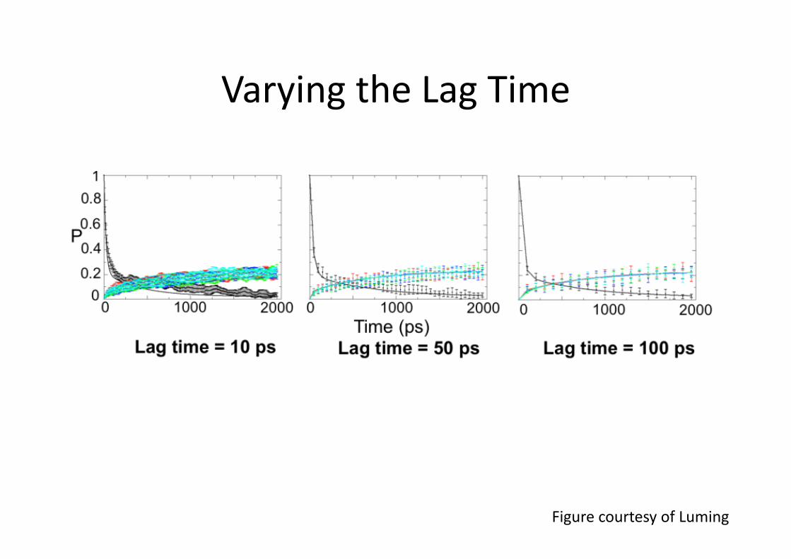
Varying the Lag TimeVarying the Lag Time
Figure courtesy of Luming
Frank Noé’s ImplementationFrank Noé s Implementation
• A simplified version of Chapman‐Kolmogorov test
C id l h li f h di l• Considers only the equality of the diagonal term (i.e. self‐transition probability) of:
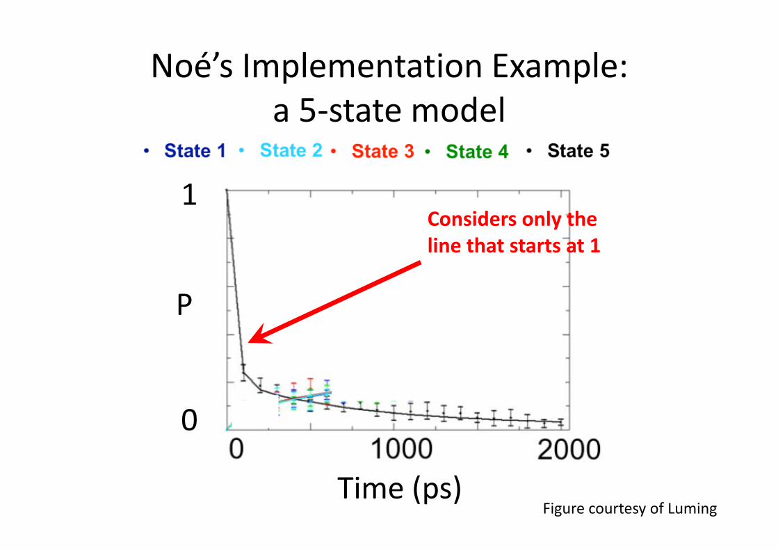
Noé’s Implementation Example:a 5‐state model
1C id l hConsiders only the line that starts at 1
P
0
Time (ps)Figure courtesy of Luming

Noé’s Implementation Example:a 2‐state model
J. Chem. Phys. 134, 174105 (2011)© 2011 American Institute of Physics

Continuous n‐dimensional variable
Discrete “1‐dimentional” variable
State: [1,2,1,2,2,2,2,3,4,4,4,4,4,4,4,4,4,4,4,4,4,5,5,5,5,5,5,5,7,7,7,6,7,6,5,6,5,5,5,4, ...]
J. Chem. Phys. 134, 174105 (2011)© 2011 American Institute of Physics

Initial low-energy backtracking pathwaysInitial low energy backtracking pathways
Pre-, frayed and backtracked models
Cli b l ith
Conformations along low energy pathways
Climber algorithm
energy pathways
Unbiased MDMD simulations
MSM constructionconstruction
Backtracking mechanism

Validating the MSMValidating the MSM

Chapman-Kolmogorov testp gMSMMDMD

Four metastable states identified by MSMFour metastable states identified by MSM

Backtracking preference
Potential of Mean Force (kcal/mol)
g p
s (Å
)uc
leot
ides
S4
o D
NA
nu
S3
MSD
of t
wo
S2TS
RM S1 S2TS
RMSD of two RNA 3′-end nucleotides (Å)

Reasons for Using MSMReasons for Using MSMBiological Processes
Experiments Simulations
Bridging simulations
LimitationsNot overlap with experimental
regime
with experimental observables
MSM
