introduction to management accounting 16th edition by charles t. horngren… · 2018-09-20 · 2-b1...

Introduction to Management Accounting 16th edition by Charles T. Horngren,

Gary L. Sundem, Jeff O. Schatzberg, Dave Burgstahler Solution Manual Link full download solution manual: https://findtestbanks.com/download/introduction-to-management-

accounting-16th-edition-by-horngren-sundem-schatzberg-burgstahler-solution-manual/

Link full download test bank: https://findtestbanks.com/download/introduction-to-management-

accounting-16th-edition-by-horngren-sundem-schatzberg-burgstahler-test-bank/

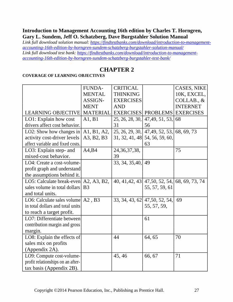
CHAPTER 2 COVERAGE OF LEARNING OBJECTIVES

FUNDA- CRITICAL CASES, NIKE

MENTAL THINKING 10K, EXCEL,

ASSIGN- EXERCISES COLLAB., &

MENT AND INTERNET

LEARNING OBJECTIVE MATERIAL EXERCISES PROBLEMS EXERCISES

LO1: Explain how cost A1, B1 25, 26, 28, 30, 47,49, 51, 53, 68

drivers affect cost behavior. 31 56

LO2: Show how changes in A1, B1, A2, 25, 26, 29, 30, 47,49, 52, 53, 68, 69, 73 activity cost-driver levels A3, B2, B3 31, 32, 41, 48 54, 56, 59, 60,

affect variable and fixed costs. 63

LO3: Explain step- and A4,B4 24,36,37,38, 75

mixed-cost behavior. 39

LO4: Create a cost-volume- 33, 34, 35,40, 49

profit graph and understand

the assumptions behind it.

LO5: Calculate break-even A2, A3, B2, 40, 41,42, 43 47,50, 52, 54, 68, 69, 73, 74 sales volume in total dollars B3 55, 57, 59, 61

and total units.

LO6: Calculate sales volume A2 , B3 33, 34, 43, 62 47,50, 52, 54, 69 in total dollars and total units 55, 57, 59,

to reach a target profit.

LO7: Differentiate between 61

contribution margin and gross

margin.

LO8: Explain the effects of 44 64, 65 70 sales mix on profits

(Appendix 2A).

LO9: Compute cost-volume- 45, 46 66, 67 71 profit relationships on an after-

tax basis (Appendix 2B).

Copyright ©2014 Pearson Education, Inc., Publishing as Prentice Hall. 27

https://findtestbanks.com/download/introduction-to-management-accounting-16th-edition-by-horngren-sundem-schatzberg-burgstahler-solution-manual/

https://findtestbanks.com/download/introduction-to-management-accounting-16th-edition-by-horngren-sundem-schatzberg-burgstahler-solution-manual/

https://findtestbanks.com/download/introduction-to-management-accounting-16th-edition-by-horngren-sundem-schatzberg-burgstahler-test-bank/

https://findtestbanks.com/download/introduction-to-management-accounting-16th-edition-by-horngren-sundem-schatzberg-burgstahler-test-bank/

CHAPTER 2

Introduction to Cost Behavior and Cost-Volume Relationships

2-A1 (20-25 Min.)

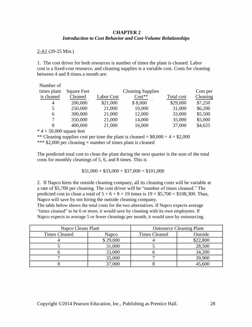
1. The cost driver for both resources is number of times the plant is cleaned. Labor cost is a fixed-cost resource, and cleaning supplies is a variable cost. Costs for cleaning between 4 and 8 times a month are:

Number of

times plant Square Feet Cleaning Supplies Cost per is cleaned Cleaned Labor Cost Cost** Total cost Cleaning

4 200,000*

$21,000 $ 8,000***

$29,000 $7,250 5 250,000 21,000 10,000 31,000 $6,200 6 300,000 21,000 12,000 33,000 $5,500

7 350,000 21,000 14,000 35,000 $5,000

8 400,000 21,000 16,000 37,000 $4,625

* 4 × 50,000 square feet

** Cleaning supplies cost per time the plant is cleaned = $8,000 ÷ 4 = $2,000

*** $2,000 per cleaning × number of times plant is cleaned

The predicted total cost to clean the plant during the next quarter is the sum of the total costs for monthly cleanings of 5, 6, and 8 times. This is

$31,000 + $33,000 + $37,000 = $101,000

2. If Napco hires the outside cleaning company, all its cleaning costs will be variable at

a rate of $5,700 per cleaning. The cost driver will be “number of times cleaned.” The predicted cost to clean a total of 5 + 6 + 8 = 19 times is 19 × $5,700 = $108,300. Thus,

Napco will save by not hiring the outside cleaning company. The table below shows the total costs for the two alternatives. If Napco expects average

“times cleaned” to be 6 or more, it would save by cleaning with its own employees. If

Napco expects to average 5 or fewer cleanings per month, it would save by outsourcing.

Napco Cleans Plant Outsource Cleaning Plant

Times Cleaned Napco Times Cleaned Outside

4 $ 29,000 4 $22,800

5 31,000 5 28,500

6 33,000 6 34,200

7 35,000 7 39,900

8 37,000 8 45,600


2-A2 (20-25 min.)

1. Let N = number of units

Sales = Fixed expenses + Variable expenses + Net income

$1.00 N = $4,000 + $.68 N + 0

$.32 N = $4,000

N = 12,500 units

Let S = sales in dollars

S = $4,000 + .68 S + 0 .32 S = $4,000 S

= $12,500

Alternatively, the 12,500 units may be multiplied by the $1.00 to obtain $12,500.

In formula form:

In units

Fixed costs + Net income =

($4,000 + 0) = 12,500 units

Contribution margin per unit

$.32

In dollars

($4,000 + 0)

Fixed costs + Net income = = $12,500

Contribution margin percentage .32

2. The quick way: (45,000 – 12,500) × $.32 = $10,400

Compare income statements:

Break-even Point Increment Total

Volume in units 12,500 32,500 45,000

Sales $12,500 $32,500 $45,000

Deduct expenses:

Variable 8,500 22,100 30,600

Fixed 4,000 --- 4,000

Total expenses 12,500 22,100 34,600

Effect on net income $ 0 $ 10,400 $ 10,400

3. Total fixed expenses would be $4,000 + $1,600 = $5,600


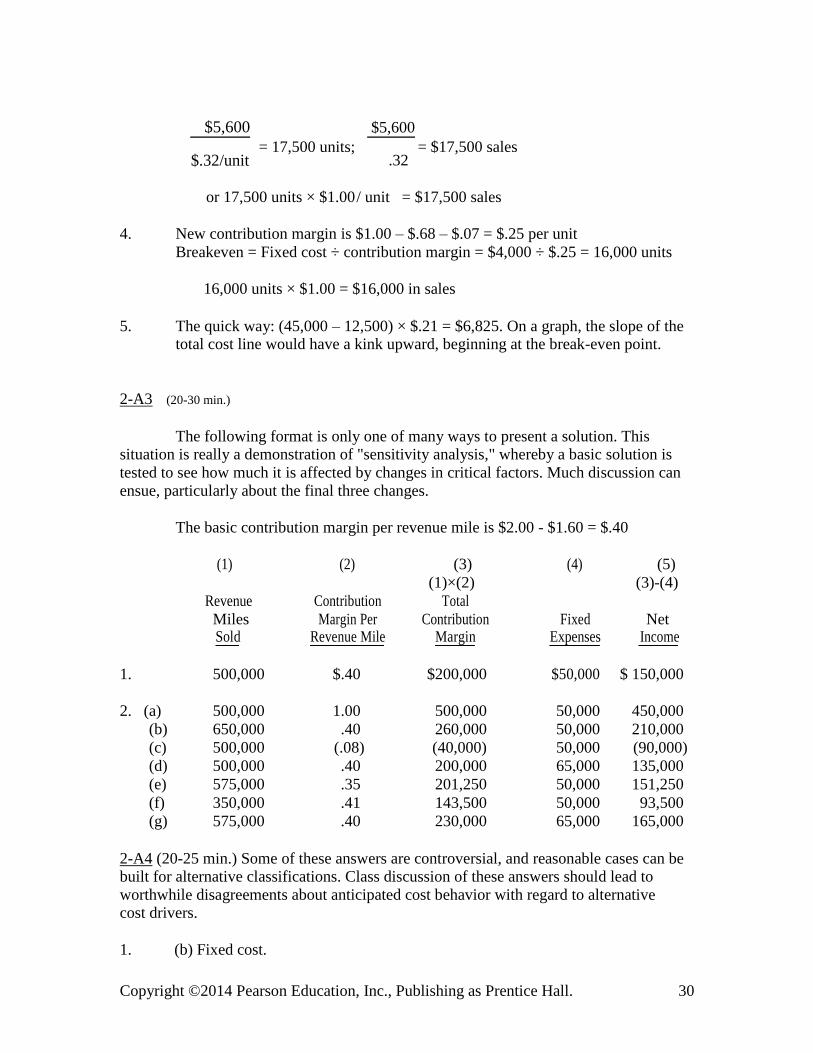
$5,600

= 17,500 units;

$5,600

= $17,500 sales $.32/unit .32

or 17,500 units × $1.00 / unit = $17,500 sales

4. New contribution margin is $1.00 – $.68 – $.07 = $.25 per unit

Breakeven = Fixed cost ÷ contribution margin = $4,000 ÷ $.25 = 16,000 units

16,000 units × $1.00 = $16,000 in sales

5. The quick way: (45,000 – 12,500) × $.21 = $6,825. On a graph, the slope of the total cost line would have a kink upward, beginning at the break-even point.

2-A3 (20-30 min.)

The following format is only one of many ways to present a solution. This situation is really a demonstration of "sensitivity analysis," whereby a basic solution is

tested to see how much it is affected by changes in critical factors. Much discussion can

ensue, particularly about the final three changes.

The basic contribution margin per revenue mile is $2.00 - $1.60 = $.40

(1) (2) (3) (4) (5) (1)×(2) (3)-(4)

Revenue Contribution Total

Miles Margin Per Contribution Fixed Net Sold Revenue Mile Margin Expenses Income

1. 500,000 $.40 $200,000 $50,000 $ 150,000

2. (a) 500,000 1.00 500,000 50,000 450,000

(b) 650,000 .40 260,000 50,000 210,000

(c) 500,000 (.08) (40,000) 50,000 (90,000)

(d) 500,000 .40 200,000 65,000 135,000

(e) 575,000 .35 201,250 50,000 151,250

(f) 350,000 .41 143,500 50,000 93,500

(g) 575,000 .40 230,000 65,000 165,000

2-A4 (20-25 min.) Some of these answers are controversial, and reasonable cases can be built for alternative classifications. Class discussion of these answers should lead to

worthwhile disagreements about anticipated cost behavior with regard to alternative cost drivers.

1. (b) Fixed cost.


2. (d) Step cost.

3. (a) Variable cost with respect to revenue.

4. (a) Variable cost with respect to miles flown.

5. (c) Mixed cost with respect to miles driven.

6. (b) Fixed cost.

7. (b) Fixed cost.

8. (b) Fixed cost.

9. (a) Variable cost with respect to cases of 7-Up.

10. (b) Fixed cost.

11. (b) Fixed cost.


2-B1 (20-25 Min.) 1. The cost driver for both resources is number of times the restaurant is cleaned.

Labor cost is a fixed-cost resource, and cleaning supplies is a variable cost. Costs for cleaning between 35 and 50 times are:

Square Cleaning

Times Feet Labor Supplies Total Cost per Cleaned Cleaned Cost Cost** Cost Cleaning

35 210,000*

$21,000 $ 16,800 $37,800 $1,080 40 240,000 21,000 19,200 40,200 $1,005 45 270,000 21,000 21,600 42,600 $ 947

50 300,000 21,000 24,000 45,000 $ 900

* 35 × 6,000 ** The cost of cleaning supplies per cleaning = $16,800 ÷ 35 = $480 per cleaning. The cost

per square foot is $480 ÷ $6,000 = $.08 or $16,800 ÷ 210,000 = $.08. The total cleaning

supplies cost is either $480 × number of cleanings or $.08 × square feet cleaned.

The predicted total cost to clean during the November and December is the sum of the total costs for monthly cleanings of 45 and 50 times. This is

$42,600 + $45,000 = $87,600

2. If Applejack hires the outside cleaning company, all its cleaning costs will be variable at a rate of $0.25 per square foot cleaned. The predicted cost to clean a total

of 45 + 50 = 95 times is 95 × 6,000 × $0.25 = $142,500. Thus, Applejack will not save by hiring the outside cleaning company.

To determine whether outsourcing is a good decision on a permanent basis, Applejack

needs to know the expected demand for the cost driver over an extended time frame. As

the following table shows, outsourcing becomes less attractive when cost driver levels

are high. If average demand for cleaning is expected to be more than the number of

cleanings at which the cost of outsourcing equals the internal cost, Applejack should

continue to do its own cleaning. This point is C cleanings, where:

$.25 × C × 6,000 = $21,000 + ( $.08 × C × 6,000)

C = $21,000 ÷ ($.17× 6,000) = 20.588 cleanings Applejack should also consider such factors as quality and cost control when an outside cleaning company is used.

(1) Times (2) Square Feet (3) Applejack Outside Cleaning Cost

Cleaned Cleaned Total Cleaning Cost*

$.25 × (2)

35 210,000 $37,800 $52,500

40 240,000 40,200 60,000

45 270,000 42,600 67,500

50 300,000 45,000 75,000

* From requirement 1, total cost is $21,000 + $.08 x square feet cleaned


2-B2 (15-25 min.)

1. $2,340 ÷ ($30 - $12) = 130 child-days or 130 × $30 = $3,900 revenue.

2. 176 × ($30 - $12) - $2,340 = $3,168 - $2,340 = $828

3. a. 198 × ($30 - $12) - $2,340 = $3,564 - $2,340 = $1,224 or (22 × $18) + $828 = $396 + $828 = $1,224

b. 176 × ($30 - $14) - $2,340 = $2,816 - $2,340 = $476 or $828 - ($2 × 176) = $476

c. $828 - $220 = $608

d. [(9.5 × 22) × ($30 - $12)] - ($2,340 + $300) = $3,762 - $2,640 = $1,122

e. [(7 × 22) × ($33 - $12)] - $2,340 = $3,234 - $2,340 = $894

2-B3 (15-20 min.)

1.

$9,100

=

$9,100

= 1,300 units

($25 - $18) $7

2. Contribution margin ratio: ($43,000 $30,100) = 30% $43,000

$8,400 ÷ 30% = $28,000

3. ($30,400 + $8,000) = $38,400 = 2,400 units ($29 - $13)$16

4. ($51,000 - $18,000) × (120%) = $39,600 contribution margin;

$39,600 - $18,000 = $21,600

5. New contribution margin: $48 - ($36 - 25% of $36)

= $48 - ($36 - $9) = $21;

New fixed expenses: $106,000 × 115% = $121,900;

($121,900 + $23,000) = $144,900 = 6,900 units $21 $21


2-B4 (20-25 min.)

The following classifications are open to debate. With appropriate assumptions,

other answers could be equally supportable. For example, in #2, the health insurance

would be a fixed cost if the number of employees will not change. This problem provides

an opportunity to discuss various aspects of cost behavior. Students should make an

assumption regarding the time period involved. For example, if the time period is short,

say one month, more costs tend to be fixed. Over longer periods, more costs are variable.

They also must assume something about the nature of the cost. For example, consider #4.

Repairs and maintenance are often thought of as a single cost. However, repairs are more

likely to vary with the amount of usage, making them variable, while maintenance is

often on a fixed schedule regardless of activity, making them fixed.

Another important point to make is the cost/benefit criterion applied to determining “true” cost behavior. A manager may accept a cost driver that is plausible

but may have less reliability than an alternative due to the cost associated with maintaining data for the more reliable cost driver.

Cost Cost Behavior Likely Cost Driver(s)

1. X-ray operating cost Mixed Number of x-rays

2. Insurance Step (or variable) Number of employees

3. Cancer research Fixed

4. Repairs Variable Number of patients

5. Training cost Fixed

6. Depreciation Fixed

7. Consulting Fixed

8. Nursing supervisors Step Number of nurses, patient-days


2-1 This is a good characterization of cost behavior. Identifying cost drivers will identify activities that affect costs, and the relationship between a cost driver and costs specifies how the cost driver influences costs.

2-2 Two rules of thumb to use are: a. Total fixed costs remain unchanged regardless of changes in cost-driver activity level. b. The per-unit variable cost remains unchanged regardless of changes in cost-driver activity level.

2-3 Examples of variable costs are the costs of merchandise, materials, parts, supplies, sales commissions, and many types of labor. Examples of fixed costs are real estate taxes, real estate insurance, many executive and supervisor salaries, and space rentals.

2-4 Fixed costs, by definition, do not vary in total as volume changes within the relevant

range and during the time period specified (a month, year, etc.). However, when the cost-

driver level is outside the relevant range (either less than or greater than the limits)

management must decide whether to decrease or increase the capacity of the resource,

expressed in cost-driver units. In the long run, all costs are subject to change. For

example, the costs of occupancy such as a long-term non-cancellable lease cannot be

changed for the term of the lease, but at the end of the lease management can change this

cost. In a few cases, fixed costs may be changed by entities outside the company rather

than by internal management – an example is the fixed, base charge for some utilities that

is set by utility commissions.

2-5 Yes. Fixed costs per unit change as the volume of activity changes. Therefore, for fixed cost per unit to be meaningful, you must identify an appropriate volume level. In contrast, total fixed costs are independent of volume level.

2-6 No. Cost behavior is much more complex than a simple dichotomy into fixed or

variable. For example, some costs are not linear, and some have more than one cost driver. Division of costs into fixed and variable categories is a useful simplification, but

it is not a complete description of cost behavior in most situations.

2-7 No. The relevant range pertains to both variable and fixed costs. Outside a relevant range, some variable costs, such as fuel consumed, may behave differently per unit of activity volume.

2-8 The major simplifying assumption is that we can classify costs as either variable or fixed with respect to a single measure of the volume of output activity.

2-9 The same cost may be regarded as variable in one decision situation and fixed in a

second decision situation. For example, fuel costs are fixed with respect to the addition of one more passenger on a bus because the added passenger has almost no effect on total

fuel costs. In contrast, total fuel costs are variable in relation to the decision of whether to add one more mile to a city bus route.


2-10 No. Contribution margin is the excess of sales over all variable costs, not fixed costs. It may be expressed as a total, as a ratio, as a percentage, or per unit.

2-11 A "break-even analysis" does not describe the real value of a CVP analysis, which shows profit at any volume of activity within the relevant range. The break-even point is

often only incidental in studies of cost-volume relationships. CVP analysis predicts how

managers’ decisions will affect sales, costs, and net income. It can be an important part of a company’s planning process.

2-12 No. break-even points can vary greatly within an industry. For example, Rolls Royce has a much lower break-even volume than does Honda (or Ford, Toyota, and other high-volume auto producers).

2-13 No. The CVP technique you choose is a matter of personal preference or convenience. The equation technique is the most general, but it may not be the easiest to apply. All three techniques yield the same results.

2-14 Three ways of lowering a break-even point, holding other factors constant, are:

decrease total fixed costs, increase selling prices, and decrease unit variable costs.

2-15 No. In addition to being quicker, incremental analysis is simpler. This is important because it keeps the analysis from being cluttered by irrelevant and potentially confusing data.

2-16 Operating leverage is a firm's ratio of fixed to variable costs. A highly leveraged company has relatively high fixed costs and low variable costs. Such a firm is risky

because small changes in volume lead to large changes in net income. This is good when

volume increases but can be disastrous when volumes fall.

2-17 An increase in demand for a company’s products will drive almost all other cost-

driver levels higher. This will cause cost drivers to exceed capacity or the upper end of

the relevant range for its fixed-cost resources. Since fixed-cost resources must be

purchased in “chunks” of capacity, the proportional increase in cost may exceed the

proportional increase in the use of the related cost-driver. Thus cost per cost-driver unit

may increase.

2-18 The margin of safety shows how far sales can fall before losses occur – that is before the company reaches the break-even sales level.

2-19 No. In retailing, the contribution margin is likely to be smaller than the gross

margin. For instance, sales commissions are deducted in computing the contribution margin but not the gross margin. In manufacturing companies the opposite is likely to be

true because there are many fixed manufacturing costs deducted in computing gross margin.


2-20 No. CVP relationships pertain to both profit-seeking and nonprofit organizations. In particular, managers of nonprofit organizations must deal with tradeoffs between

variable and fixed costs. To many government department managers, lump-sum budget appropriations are regarded as the available revenues.

2-21 Contribution margin could be lower because the proportion of sales of the product bearing the higher unit contribution margin is lower than the proportion budgeted.

2-22

Target income before =

Target after-tax net income

income taxes

1 - tax rate

2-23

Change in = Change in volume × Contribution margin × (1 - tax rate)

net income in units per unit

2-24 The fixed salary portion of the compensation is a fixed cost. It is independent of

how much is sold. In contrast, the 5% commission is a variable cost. It varies directly with the amount of sales. Because the compensation is part fixed cost and part variable

cost, it is considered a mixed cost.

2-25 The key to determining cost behavior is to ask, “If there is a change in the level of

the cost driver, will the total cost of the resource change immediately?” If the answer is

yes, the resource cost is variable. If the answer is no, the resource cost is fixed. Using

this question as a guide, the cost of advertisements is normally variable as a function of

the number of advertisements. Note that because the number of advertisements may not

vary with the level of sales, advertising cost may be fixed with respect to the cost driver

“level of sales.” Salaries of marketing personnel are a fixed cost. Travel costs and

entertainment costs can be either variable or fixed depending on the policy of

management. The key question is whether it is necessary to incur additional travel and

entertainment costs to generate added sales.

2-26 The key to determining cost behavior is to ask, “If there is a change in the level of

the cost driver, will the total cost of the resource change immediately?” If the answer is

yes, the resource cost is variable. If the answer is no, the resource cost is fixed. Using this

question as a guide, the cost of labor can be fixed or variable as a function of the number

of hours worked. Regular wages may be fixed if there is a commitment to the laborers

that they will be paid for normal hours regardless of the workload. However, overtime

and temporary labor wages are variable. The depreciation on plant and machinery is not a

function of the number of machine hours used and so this cost is fixed.


2-27 Suggested value chain functions are listed below.

New Positioning

New Products New Technology Strategies New Pricing

Marketing R & D Marketing Marketing

R & D Design Support

Design functions

2-28 (10-15 min.)

Situation Best Cost Driver Justification

1. Number of Setups Because each setup takes the same amount of time, the best cost driver is number of setups. Data is both

plausible, reliable, and easy to maintain.

2. Setup Time Longer setup times result in more consumption of mechanics’ time. Simply using number of setups as

in situation 1 will not capture the diversity

associated with this activity.

3. Cubic Feet Assuming that all products are stored in the warehouse for about the same time (that is

inventory turnover is about the same for all

products), and that products are stacked, the volume

occupied by products is the best cost driver.

4. Cubic Feet Weeks If some types of product are stored for more time than others, the volume occupied must be multiplied

by a time dimension. For example, if product A

occupies 100 cubic feet for an average of 2 weeks

and product B occupies only 40 cubic feet but for an

average of 10 weeks, product B should receive

twice as much allocation of warehouse occupancy

costs.

5. Number of Orders Because each order takes the same amount of time, the best cost driver is number of orders. Data is both

plausible, reliable, and easy to maintain.

6. Number of Orders Each order is for different types of products but there is not diversity between them in terms of the

time it takes to process the order. (If there was

variability in the number of product types ordered,

the best driver would be number of order line

items.)


2-29 (5-10 min.)

1. Contribution margin = $960,000 - $533,000 = $427,000

Net income = $427,000 - $310,000 = $117,000

2. Variable expenses = $550,000 - $300,000 = $250,000

Fixed expenses = $300,000 - $ 46,000 = $254,000

3. Sales = $500,000 + $520,000 = $1,020,000

Net income = $520,000 - $200,000 = $320,000

2-30 (5-10 min.)

The $278,000 annual advertising fee is a fixed cost. The $6,100 cost for each advertisement is a variable cost.

If the total number of ads is 46 the total cost of advertising is

$278,000 + 46 × $6,100 = $558,600

If the total number of ads is 92 the total cost of advertising is

$278,000 + 92 × $6,100 = $839,200.

The total cost of advertising does not double in response to a doubling of the number of ads because the fixed costs do not change.

2-31 (5-10 min.)

With respect to the cost driver sales dollars, the $3,200,000 annual salaries of sales personnel is a fixed cost. The sales commissions, travel costs, and entertainment costs are variable costs.

If the total sales dollars is $24 million, the total cost of the selling activity is

$3,200,000 + .20 × $24,000,000 = $8,000,000

If the total sales dollars is only $12 million, the total cost of the selling activity is

$3,200,000 + .20 × $12,000,000 = $5,600,000.

The total cost of the selling activity does not decrease by 50% when the cost driver decreases by 50% because the fixed costs do not change.


2-32 (10-20 min.)

1. d = c × (a - b)

$750,000 = 125,000 × ($26 - b) b = $20 f = d - e

= $750,000 - $675,000 = $75,000

2. d = c × (a - b)

= 100,000 × ($10 - $6) = $400,000

f = d - e

= $400,000 - $320,000 = $80,000

3. c = d ÷ (a - b)

= $63,000 ÷ $3 = 21,000 units

e = d - f

= $63,000 - $14,000 = $49,000

4. d = c × (a - b)

= 60,000 × ($30 - $20)

= $600,000

e = d - f

= $600,000 - $12,000 = $588,000

5. d = c × (a - b)

$172,000 = 86,000 × (a - $12)

a = $14

f = d - e

= $172,000 - $125,000 = $47,000


2-33 (10 min.)

Using the graph above, the estimated breakeven point in total units sold is about 80,000 (where revenue = $800,000 and total costs = $320,000 + $480,000 = $800,000). The

estimated net income for 100,000 units sold is $80,000 (revenue of $1,000,000 – total costs of $320,000 + $600,000 = $920,000).


2-34 (10 min.)

Using the graph above, the estimated breakeven point in total units sold is about 60,000

(actual breakeven volume is 58,800). The estimated net loss for 50,000 units sold is

$88,000 (revenue of $1,500,000 – total cost of $1,588,000 or CM of $500,000 less fixed

cost of $588,000).


2-35 (20–25 min.)

Square Labor Cost per Supplies Cost per

Feet Labor Cost Square Foot Supplies Cost Square Foot

100,000 $24,000 $ 0.240 $ 5,000 $0.050

125,000 24,000 $ 0.192 6,250 0.050

150,000 24,000 $ 0.160 7,500 0.050

175,000 24,000 $ 0.137 8,750 0.050

200,000 24,000 $ 0.120 10,000 0.050

Labor Cost per Square Foot

$0.30

$0.25

$0.20

$0.15

$0.10

Fixed-Cost

$0.05

per Unit

$- Behavior

100,000 125,000 150,000 175,000 200,000

Square Feet

Supplies Cost per Square Foot

Co

st

per

Sq

uare

F

oo

t S

up

pli

es

$0.06

$0.05

$0.04

$0.03

Variable-Cost

$0.02 per Unit

Behavior

$0.01

$-

100,000 125,000 150,000 175,000 200,000

Square Feet


2-36 (20-25 min.)

Supplies

Labor Cost Per Cost per

Square Square Foot Total Labor Square Supplies Feet (Estimated) Cost Foot Cost

100,000 $0.12 $12,000 $0.06 $ 6,000

125,000 0.096 12,000 0.06 7,500

150,000 0.08 12,000 0.06 9,000

Total Labor Cost $14,000 $12,000 $10,000

$8,000

$6,000

$4,000

$2,000

$0

100,000 125,000 150,000

Square Feet

Total Supplies Cost

$10,000

$9,000 $8,000 $7,000 $6,000 $5,000 $4,000 $3,000 $2,000 $1,000

$0

100,000 125,000 150,000

Square Feet

Labor cost shows a fixed-cost behavior, while supplies cost shows a variable-cost behavior.


2-37 (5 min.) Only (b) is a step cost. (a) This is a fixed cost. The same cost applies to all volumes in the relevant range. (b) This is a true step cost. Each time 15 students are added, the cost increases by the amount of one teacher’s salary. (c) This is a variable cost that may be different per unit at different levels of

volume. It is not a step cost. Why? Because each unit of product requires a

particular amount of steel, regardless of the form in which the steel is purchased.

2-38 (5 min.) The $8,000 is a fixed cost and the $52 per unit is a variable cost. By

definition, adding a fixed cost and a variable cost together produces a mixed cost.

2-39 (10-15 min.)

1. Machining labor: G, number of units completed or labor hours

2. Raw material: B, units produced; could also be D if the company’s purchases do

not affect the price of the raw material.

3. Annual wage: C or E (depending on work levels), labor hours

4. Water bill: H, gallons of water used

5. Quantity discounts: A, amount purchased

6. Depreciation: E, capacity

7. Sheet steel: D, number of farm implements of various types

8. Salaries: F, number of solicitors

9. Natural gas bill: C, cubic feet of usage

2-40 (10 min.)

1. Let TR = total revenue

TR - .25(TR) -$45,000,000 = 0

.75(TR) = $45,000,000

TR = $60,000,000

2. Daily revenue per patient = $60,000,000 ÷ 37,500 = $1,600. This may appear high, but it includes the room charge plus additional charges for drugs, x-rays, and so forth.

2-41 (10 min.)

1. The break-even point in total revenue is fixed cost divided by the contribution-margin ratio (CMR). CMR equals 1 – Variable-Cost Ratio.

Break-even Point = Fixed Cost ÷ CMR = $42,000,000 ÷ (1 – 0.7) = $140,000,000.

2.


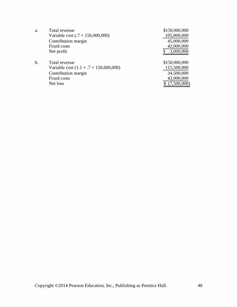
a. Total revenue $150,000,000 Variable cost (.7 × 150,000,000) 105,000,000

Contribution margin 45,000,000 Fixed costs 42,000,000 Net profit $ 3,000,000

b. Total revenue $150,000,000 Variable cost (1.1 × .7 × 150,000,000) 115,500,000

Contribution margin 34,500,000 Fixed costs 42,000,000 Net loss $ (7,500,000)


2-42 (15 min.)

a b 1. 100% Full 50% Full

Room revenue @ $54 $ 1,971,000 a

$ 985,500 b

Variable costs @ $9 328,500 164,250

Contribution margin 1,642,500 821,250 Fixed costs 900,000 900,000

Net income (loss) $ 742,500 $ (78,750)

a 100 × 365 = 36,500 rooms per year

36,500 × $54 = $1,971,000

b 50% of $1,971,000 = $985,500

2. Let N = number of rooms rented

$54N -$9N - $900,000 = 0

N = $900,000 ÷ $45 = 20,000 rooms

Percentage occupancy = 20,000 ÷ 36,500 = 54.8%

2-43 (15 min.)

1. $23. To compute this, let X be the variable cost that generates $1 million in profits:

($48 - X ) × 800,000 - $19,000,000 = $1,000,000

($48 - X) = ($1,000,000 + $19,000,000) ÷ 800,000

$48 - X = $200 ÷ 8 = $25

X = $48 - $25 = $23

2. Loss of $600,000:

($48 - $25) × 800,000 - $19,000,000

= ($23 × 800,000) - $19,000,000

= $18,400,000 - $19,000,000

= ($600,000)


2-44 (15-20 min.)

1. Let 2R = pints of raspberries and 5R = pints of strawberries sales - variable expenses - fixed expenses = zero net income

($1.05×5R) + ($1.30×2R) – ($.85×5R) – ($.90×2R) - $15,300 = 0 ($5.25 × R) + ($2.60 × R) – ($4.25 × R) – ($1.80 × R) -$15,300 = 0

$1.8 × R - $15,300 = 0 R = 8,500

2R = 17,000 pints of raspberries

5R = 42,500 pints of strawberries

2. Let S = pints of strawberries

($1.05 - $.85) × S - $15,300 = 0

.20S - $15,300 = 0

S = 76,500 pints of strawberries

3. Let R = pints of raspberries

($1.30 - $.90) × R - $15,300 = 0 ($.40 × R) - $15,300 = 0 R = 38,250 pints of raspberries

2-45 (10 min.) 1. ($1.50 × N) – ($1.20 × N) – $18,000 = $864 ÷ (1 -

.25) ($.30 × N) = $18,000 + ($864 ÷ .75) ($.30 × N) = $18,000 + $1,152

N = $19,152 ÷ $.30 = 63,840 units

2. ($1.50 × N) – ($1.20 × N) - $18,000 = $1,440 ÷ (1 - .25) ($.30 × N) = $18,000 +( $1,440 ÷ .75) ($.30 × N) = $18,000 + $1,920

N = $19,920 ÷ $.30 = 66,400 units


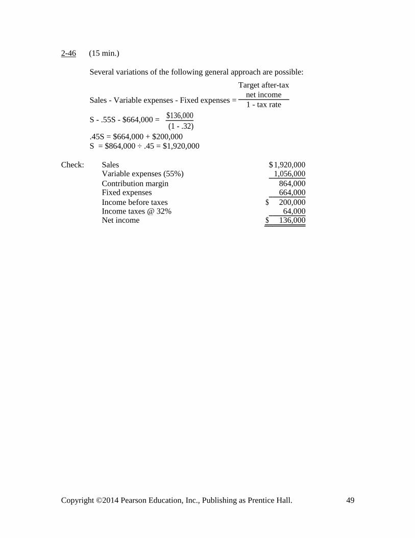
2-46 (15 min.)

Several variations of the following general approach are possible:

Target after-tax

Sales - Variable expenses - Fixed expenses = net income

1 - tax rate

S - .55S - $664,000 = $136,000

(1 - .32)

.45S = $664,000 + $200,000

S = $864,000 ÷ .45 = $1,920,000

Check: Sales $ 1,920,000 Variable expenses (55%) 1,056,000

Contribution margin 864,000 Fixed expenses 664,000

Income before taxes $ 200,000 Income taxes @ 32% 64,000 Net income $ 136,000


2-47 (40-50 min.)

1. Several variations of the following general approach are possible:

Let N = Unit Sales.

Sales - Variable expenses - Fixed expenses = Profit

$5N – $4.1N – ($3,000 + $4,000 + $3,000) = $500

$.9N - $10,000 = $500

N = $10,500 ÷ $.9 = 11,666.67 glasses of beer

Check: Sales (11,666.67 × $5) $58,333 Variable expenses (11,666.67 × $4.1) 47,833

Contribution margin 10,500 Fixed expenses 10,000 Profit $ 500

2. $5N – $4.1N - $10,000 = .05 × ($5N)

N = $10,000 ÷ ($.9 - $.25) = 15,385 glasses of beer

3. Fixed Cost ÷ (Sales price – cost of meat – cost of buns – cost of other ingredients) = # of hamburgers $1,560 ÷ ($1.24 - $.40 - $.12 - $.12) = 2,600 hamburgers

4. (3,000 × $.60) + (4,800 × $.90) - $1,560 = $1,800 + $4,320 - $1,560 = $4,560 added profit

5. $1,560 ÷ ($.60 + $.90) = 1,040 new customers are needed to breakeven on the new business.

A sensitivity analysis would help provide Terry with an assessment of the financial risks

associated with the new hamburger business. Suppose that Terry is confident that demand

for hamburgers would range between break-even ± 500 new customers and that expected

fixed costs will not change within this range. The contribution margin generated by each

new customer is $1.50 so Terry will realize a maximum loss or profit from the new

business in the range ± $1.50 × 500 = ± $750.

Another way to assess financial risk that Terry should be aware of is the company’s

operating leverage (the ratio of fixed to variable costs). A highly leveraged company has relatively high fixed costs and low variable costs. Such a firm is risky because small

changes in volume lead to large changes in net income. This is good when volume

increases but can be disastrous when volumes fall.

6. The additional cost of higher quality hamburger ingredients is .5 × $.64 = $.32. Any price for the higher quality hamburgers above the current price of $1.24 plus $.32, or

$1.56, will improve profits, assuming the same number of customers purchase hamburgers.


2-48 (30-40 min.)

1. The cost of labor and equipment rent is fixed at $21,000 per month. Cleaning supplies cost varies in proportion to the number of times the store is cleaned. The cost per cleaning is $12,000 ÷ 60 = $200.

Number of Labor & Cleaning Supplies

Times Store Rent Cost at Total Cost per Is Cleaned Cost $200 per Cleaning Cost Cleaning

35 $21,000 $7,000 $28,000 $800.00

40 21,000 8,000 29,000 725.00

45 21,000 9,000 30,000 666.67

50 21,000 10,000 31,000 620.00

55 21,000 11,000 32,000 581.82

60 21,000 12,000 33,000 550.00

The total cost of cleaning for the next quarter is:

Total cost = Total Fixed Cost + Total Variable Cost

= 3 × $21,000 + (50 + 46 + 35) × $200 per Cleaning

= $63,000 + $26,200

= $89,200

2. See the chart on the next page.

3. Costs of Super Valu Cleaning Store

Number of Labor & Cleaning Outside

Times Store Rent Supplies Total Cleaning Month Is Cleaned Cost Cost Cost Cost

June 35 $21,000 $ 7,000 $28,000 $25,200

May 46 21,000 9,200 30,200 33,120 April 50 21,000 10,000 31,000 36,000 $89,200 $94,320

Super Value will save $94,320- $89,200 = $5,120 by continuing to do its own cleaning rather than using the outside cleaning company, as shown in the above schedule.


2-49 (10-15 min.)

The budget for professional salaries for the coming year is $1,100,000.

Refined analysis:

Key professional salaries

$1,200,000 1,100,000 1,000,000

$2,000,000 $2,400,000 Billings

Simplified analysis:

Key professional salaries

$1,200,000 1,100,000 1,000,000

$2,000,000 $2,400,000 Billings

Relevant Range


2-50 (15-20 min.)

1. Microsoft: ($60,420 - $11,598) ÷ $60,420 = .81 or 81%

Procter & Gamble: ($83,503 - $40,695) ÷ $83,503) = .51 or 51%

There is very little variable cost for each unit of software sold by Microsoft, as the

variable cost percentage is only 19%. The variable cost percentage for the soap,

cosmetics, foods, and other products of Procter & Gamble is much higher at 49%.

2. Microsoft: $10,000,000 × .81 = $8,100,000

Procter & Gamble: $10,000,000 × .51 = $5,100,000

3. We know that the total contribution margin generated by any added sales will be added to the operating income. Thus, we can simply multiply the contribution margin percentage by the changes in sales to get the change in operating income.

The main assumption we make is that the sales volume remains in the relevant range so that total fixed costs do not change and unit variable cost remain unchanged. This

generally means that such predictions will apply only to small changes in volume – changes that do not cause either the addition or reduction of capacity.


2-51 (15-20 min.)

Film Refreshments Total

1. Revenue from admissions $2,250 $270 b

$ 2,520

Variable costs 1,125 a

162 c

1,287 Contribution margin $1,125 $108 $ 1,233

Fixed costs:

Auditorium rental $330 Labor 435 765 Operating income $ 468

a .50 × $2,250 = $1,125

b .12 × $2,250 = $270

c .60 × $ 270 = $162

Some labor might be exclusively devoted to refreshments. Labor might be allocated, but such a discussion is not the major point of this chapter.

Film Refreshments Total

2. Revenue from admissions $1,400.00 $ 168.00b

$ 1,568.00

Variable costs 750.00a

100.80c

850.80

Contribution margin $650.00 $ 67.20 $ 717.20

Fixed costs:

Auditorium rental $330 Labor 435 765.00 Operating income (loss) $ (47.80)

a Guarantee is $750

b .12 × $1,400 = $168

c .60 × $168 = $100.80

3. The offer would shift the risk completely to the movie producer, whereas ordinarily the theater owner bears a great deal of the risk. The owner is assured

of a specified income; the producer then reaps the reward or bears the cost of the actual attendance level.


2-52 (15 min.)

1. Let X = amount of additional fixed costs for advertising

(1,300,000 × £15) +£270,000 -.20(1,300,000 × £15) - (£7,300,000 + X) = 0

£19,500,000 + £270,000 - £3,900,000 - £7,300,000 - X = 0

X = £19,770,000 - £11,200,000

X = £8,570,000

2. Let Y = number of seats sold

£15Y + £270,000 - .20 × £15Y - £11,000,000 = £490,000

£12Y = £11,220,000

Y = 935,000 seats


2-53 (45-55 min.)

1. Exhibit A shows the relationships between the receiving activity and the

resources used. This information can now be used for cost control purposes. Knowing the two rates, gallons per part received and machine hours operated per

part received, will help operating managers predict costs. These rates are measures of productivity in the receiving department.

Exhibit A

EQUIPMENT FUEL RESOURCE

RESOURCE $24,000 ÷ 6,000 Gal. =

$45,000 $4 Per Gallon Used

1,500 Hours/30,000 Parts = 0.05 6,000 Gal./30,000 Parts = 0.2 Hours/Part Received Gal./Part Received

RECEIVING ACTIVITY

Cost Driver

Number of Parts Received, 30,000

2. When the activity level increases, the use of resources will increase. Thus, the

output measures or cost driver levels will increase – that is, total hours and total gallons. Normally, productivity rates such as gallons per part received and

hours operated per part received will not change significantly unless a) there is action taken to improve efficiency, or b) factors act to decrease efficiency.

An equation can be derived to predict total cost using the above concept.

Total Cost = Variable Cost of Fuel + Fixed Cost of Equipment = (Number of Parts Received × Gallon/Part × Price/Gallon) + $45,000

The total cost of receiving 40,000 parts is

(40,000 parts × 0.2 Gallon/Part × $4/Gallon) + $45,000 = $77,000


3. The new fuel consumption rate will be .80 × 0.2 gallons/part received = 0.16

gallons per part received. The predicted cost of receiving 30,000 parts is

(30,000 Parts × 0.16 Gallons/Part × $4.00 per Gallon) + $45,000 = $19,200 + $45,000 = $64,200.

The receiving department will not achieve the 10% cost reduction goal of $62,100

even though productivity in fuel usage improved by 20%. Although the variable

cost of fuel declines by 20%, the fixed cost of equipment does not decline at all,

and the fixed equipment costs are a large portion of the total cost of receiving.

Perhaps management should consider setting cost reduction goals in the light of

knowledge of cost behavior.

4. The new model contains productivity measures that are controllable by

operating managers who are responsible for costs incurred. As a result, management can expect higher levels exerted effort by managers as well as

improvement in cost control.

5. One refinement is to note that total fuel usage is a function of both the efficiency

in machine use as well as efficiency in fuel consumption. In terms of productivity metrics this can be expressed as follows:

Current model:

Total Fuel Cost = $/Gallon × Gallons/Part Received × Total Number of Parts Received.

Refined model: Total Fuel Cost = $/Gallon × Gallons Used/Operating Hour × Operating Hours/Part

Received × Total Number of Parts Received.

The refined model has two productivity measures instead of only one. Both these

measures are controllable by operating managers in the receiving department. As a result, management can focus effort in two areas of potential improvement. For

example, if there was a 20% improvement in both these productivity measures, the total fuel cost would be

Total fuel cost = $4/Gal. × .8 × 4 Gal./Hour Operated × .8 × .05* Hours Operated/Part Received × 30,000 Parts Received = $15,360.

* 1,500 operating hours/30,000 parts received

The predicted total cost of receiving would then be

$15,360 + $45,000 = $60,360 and the target goal would be achieved.


2-54 (20-30 min.)

Many shortcuts are available, but this solution uses the equation technique.

1. Let N = meals sold Sales - Variable expenses - Fixed expenses = Profit before taxes $18N - $9.50N - $17,000 = $8,500

N = $25,500 ÷ $8.50

N = 3,000 meals

2. $18N - $9.50N - $17,000 = $0 N = $17,000 ÷ $8.50 N = 2,000 meals

3. $22N - $11.40N - $25,420 = $8,500 N = $33,920 ÷ $10.60 N = 3,200 meals

4. Profit = ($22 × 2,550) – ($11.40 × 2,550) - $25,420 Profit = $1,610

5. Profit = ($22 × 2,800) –($11.40 × 2,800) - ($25,420 + $2,300) Profit = $29,680 - $27,720 Profit = $1,960, an increase of $350.

A shortcut, incremental approach follows:

Increase in contribution margin, 250 × $10.60 $2,650 Increase in fixed costs 2,300 Increase in profit $ 350


2-55 (10-15 min.)

1. The break-even point is $65 fixed cost $2 per day = 32.5 days 2. The break-even point is about $7 fixed cost [$2 – (.40×$2)] = 5.8 days 3. Let N = 50 days rented.

Under the traditional system the total income is

Revenue – variable cost – fixed cost = $2×N - $0×N - $65

= $100 - $65

= $35

Under the new system the income is

Revenue – variable cost – fixed cost = $2×N – (.4×$2×N) - $7

= $100 - $40 - $7

= $ 53 4. Under the traditional system there would be a loss of

$53. $2×6 - $65 = ($53)

Under the new system there would be an income of $.20.

$2×6 – (.4×$2×6) - $7 = $.20

5. Blockbuster reduces its risk substantially under the new system because

it reduces its fixed cost.


2-56 (10-15 min.) Amounts are in millions (rounded with slight rounding errors).

Net sales (.9 × $82,559) $74,303

Variable costs: Cost of goods sold (.9 × $40,768) 36,691

Contribution margin 37,612

Fixed costs: Selling, administrative, and general expenses 25,973

Operating income $11,639

The percentage decrease in operating income would be 1 – ($11,639 $15,818) = 1

– .736 or 26.4%, compared with a 10% decrease in sales. The contribution margin would decrease by 10% or .10 × ($82,559 - $40,768) = $4,179 million.

Because fixed costs would not change (assuming the new volume is within the

relevant range), operating income would also decrease by $4,179 million, from $15,818 million to $11,639 million.

Because of the existence of fixed costs, the percentage decrease in operating

income will exceed the percentage decrease in sales. If all costs had been

variable, fixed costs would have decreased by an additional .10 × $25,973 =

$2,597 million, making operating income $11,639 + $2,597 = $14,236 million, a

10% decrease from the 2011 operating income of $15,818 million.


2-57 (15-25 min.)

1. Average revenue per person $8.00 + 4($.50) = $10.00

Total revenue, 200 @ $10.00 = $2,000 Rent 950

Total available for prizes and operating income $1,050

The church could award cash prizes of $1,050 and break even.

2. Number of persons 50 200 350

Total revenue @ $10.00 $ 500 $ 2,000 $3,500

Fixed costs

Rent $ 950 Prizes 1,050 2,000 2,000 2,000 Operating income (loss) $(1,500) $ 0 $ 1,500

Note how "leverage" works. Being highly leveraged means having relatively high fixed costs. In this case, there are no variable costs. Therefore, the revenue

is the same as the contribution margin. As volume departs from the break-even point, operating income is affected at a significant rate of $10.00 per person.

3. Number of persons 50 200 350

Revenue $ 500 $ 2,000 $3,500 Variable costs 50 200 350

Contribution margin $ 450 $ 1,800 $3,150

Fixed costs: Rent $ 700 Prizes 1,050 1,750 1,750 1,750 Operating income (loss) $(1,300) $ 50 $1,400

The risk is lower with the revised cost structure because of lower operating

leverage – fixed costs are lower and variable costs are higher. Some of the risk

has been shifted to the hotel. As a result, when attendance is low, the parish will

not lose as much money, and when attendance is high, the parish will not make

as much money. For example, the income at 350 persons is $1,400 versus

$1,500 and the loss at 50 persons is $(1,300) instead of $(1,500).


2-58 (10-20 min.)

1. To compute eBay’s operating income, we need to know fixed and variable costs. We are given that its fixed costs are $37 million. Variable costs in the first quarter of 2001 were:

Operating expenses - Fixed costs

$123 million - $37 million

= Variable costs

= $86 million

Variable costs were $86 million ÷ $154 million = 55.84% of sales. If this percentage also applied to 2002, variable costs in 2002 should have been 55.84% × $245 million = 136.8 million.

Since sales increased by 1 – ($245 million ÷ $154 million) = 59.09% in 2002, variable costs should also have increased by 59.09%:

2002 variable costs = 1.5909 × $86 million = $136.8 million

Therefore, we calculate 2002 operating income as follows:

operating income = revenues – variable cost – fixed cost

=$245 million - $136.8 million - $37 million = $71.2 million

This is a 130% increase in operating income:

($71.2 million ÷ $31 million) – 1 = 130%

2. When sales increased 59%, operating income increased by 130%. This is an example

of the effect of operating leverage. The variable cost percentage is approximately $86 ÷

$154 = 56%. Thus, the contribution margin percentage is 100% - 56% = 44%. Every

dollar of sales generates $.44 of operating income. The sales increase of $245 million -

$154 million = $91 million generated $91 million × 44% = $40 million of operating

income, while the original $154 million of sales had generated only $31 million of

operating income. This is because the same $37 million of fixed cost applied at both

level of sales. The additional $91 million of sales caused no additional fixed costs, so its

total contribution margin all becomes operating income.


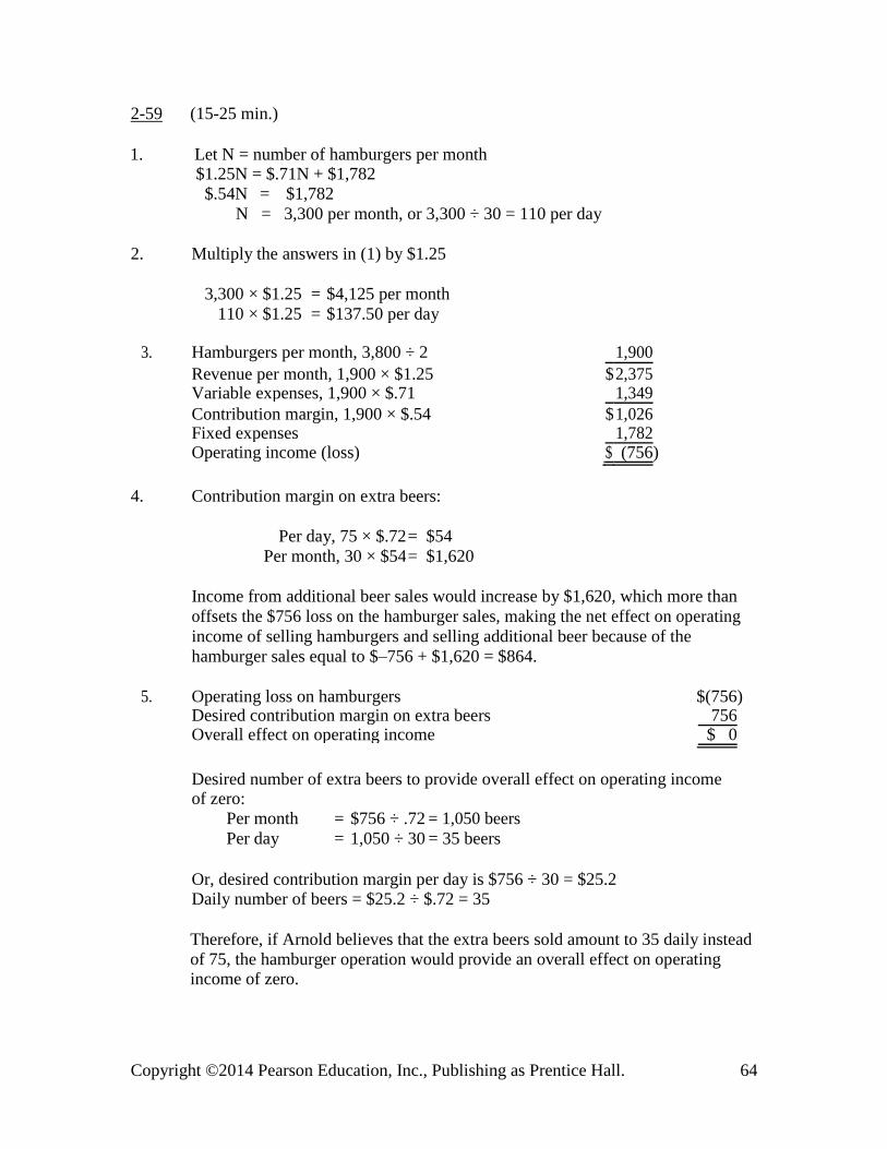
2-59 (15-25 min.)

1. Let N = number of hamburgers per month $1.25N = $.71N + $1,782 $.54N = $1,782

N = 3,300 per month, or 3,300 ÷ 30 = 110 per day

2. Multiply the answers in (1) by $1.25

3,300 × $1.25 = $4,125 per month

110 × $1.25 = $137.50 per day

3. Hamburgers per month, 3,800 ÷ 2 1,900

Revenue per month, 1,900 × $1.25 $ 2,375 Variable expenses, 1,900 × $.71 1,349

Contribution margin, 1,900 × $.54 $ 1,026 Fixed expenses 1,782 Operating income (loss) $ (756)

4. Contribution margin on extra beers:

Per day, 75 × $.72 = $54

Per month, 30 × $54 = $1,620

Income from additional beer sales would increase by $1,620, which more than

offsets the $756 loss on the hamburger sales, making the net effect on operating

income of selling hamburgers and selling additional beer because of the

hamburger sales equal to $–756 + $1,620 = $864.

5. Operating loss on hamburgers $(756) Desired contribution margin on extra beers 756 Overall effect on operating income $ 0

Desired number of extra beers to provide overall effect on operating income of zero:

Per month = $756 ÷ .72 = 1,050 beers

Per day = 1,050 ÷ 30 = 35 beers

Or, desired contribution margin per day is $756 ÷ 30 = $25.2 Daily number of beers = $25.2 ÷ $.72 = 35

Therefore, if Arnold believes that the extra beers sold amount to 35 daily instead

of 75, the hamburger operation would provide an overall effect on operating income of zero.


2-60 (15-20 min.) Note in requirements 2 and 3 how the percentage declines exceed the 15% budget reduction.

1. Let N = number of persons Revenue - variable expenses - fixed expenses = 0

$900,000 - $5,000N - $280,000 = 0 5,000N = $900,000 - $280,000

N = $620,000 ÷ $5,000

N = 124 persons

2. Revenue is now; .85($900,000)= $765,000 $765,000 - $5,000N - $280,000 = 0

$5,000N = $765,000 - $280,000 N = $485,000 ÷ $5,000

N = 97 persons

Percentage drop: (124 - 97) ÷ 124 = 21.8%

3. Let y = supplement per person

$765,000 - 124y - $280,000 = 0

124y = $765,000 - $280,000 y = $485,000 ÷ 124 y = $3,911

Percentage drop: ($5,000 - $3,911) ÷ $5,000 = 21.8%

Regarding requirements 2 and 3, note that the cut in service can be measured by

a formula:

% cut in service = % budget change ÷ % variable cost

The variable-cost ratio is $620,000 ÷ $900,000 = 68.9%

% cut in service = 15% ÷ 68.9% = 21.8%


2-61 (15-20 min.) Answers are in millions.

1. Sales $6,022

Variable costs:

Variable costs of goods sold $3,735 Variable other operating expenses 487 4,222 Contribution margin $ 1,800

Contribution margin percentage = $1,800 $6,022 = 29.9%

The contribution margin equals sales less all variable costs, while gross margin equals

sales less cost of goods sold. The variable costs include part of the costs of goods sold

and also part of the other operating costs. Note that contribution margin can be either

larger than or smaller than the gross margin. If most of the cost of goods sold and a good

portion of the other operating costs are variable, then variable costs may exceed the cost

of goods sold, and the contribution margin will be smaller than the gross margin.

However, if a large portion of both the cost of goods sold and the other expenses are

fixed, cost of goods sold may exceed the variable cost, resulting in the contribution

margin exceeding gross margin.

2. Predicted sales increase = $6,022 × .10 = $602.20 Additional contribution margin = $602.20 × .299 = $180 Fixed costs do not change Predicted operating loss = $(600) + $180 = $(420) Percentage

decrease in operating loss = $180 $(600) = 30%

Note that a 10% increase in sales would decrease the operating loss by 30%.

3. Assumptions include:

Expenses can be classified into variable and fixed categories that completely describe their behavior within the relevant range. Costs and revenues are linear within the relevant range.

Predicted sales volume is within the relevant range. Efficiency and productivity are

unchanged. Sales mix is unchanged. Changes in inventory levels are insignificant.


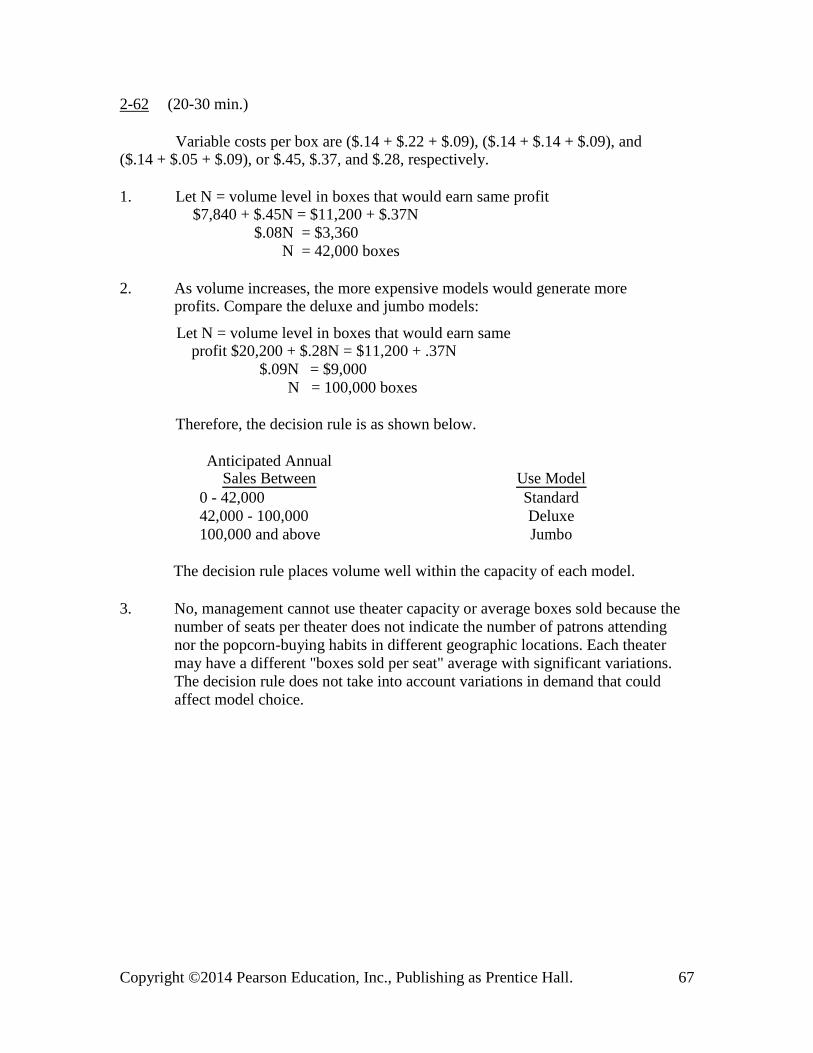
2-62 (20-30 min.)

Variable costs per box are ($.14 + $.22 + $.09), ($.14 + $.14 + $.09), and ($.14 + $.05 + $.09), or $.45, $.37, and $.28, respectively.

1. Let N = volume level in boxes that would earn same profit $7,840 + $.45N = $11,200 + $.37N

$.08N = $3,360

N = 42,000 boxes

2. As volume increases, the more expensive models would generate more profits. Compare the deluxe and jumbo models:

Let N = volume level in boxes that would earn same profit $20,200 + $.28N = $11,200 + .37N

$.09N = $9,000

N = 100,000 boxes

Therefore, the decision rule is as shown below.

Anticipated Annual Sales Between Use Model

0 - 42,000 Standard

42,000 - 100,000 Deluxe

100,000 and above Jumbo

The decision rule places volume well within the capacity of each model.

3. No, management cannot use theater capacity or average boxes sold because the

number of seats per theater does not indicate the number of patrons attending

nor the popcorn-buying habits in different geographic locations. Each theater

may have a different "boxes sold per seat" average with significant variations.

The decision rule does not take into account variations in demand that could

affect model choice.


2-63 (10-15 min.)

1. Kellogg’s has the higher fixed cost, while Post has the higher variable cost. Thus, the

contribution margin for Kellogg’s will be higher. Kellogg’s will have more risk. Its profits increase faster as sales increase, but its profits decrease faster (or losses increase

faster) as sales decrease.

2. Post provides more inventive to its sales force to increase sales. For each $1 of increased sales, Post pays more of that increase to the sales force, while Kellogg’s retains more of the increase for the company’s profit.

3. A possible negative of the increased inventive for the Post sales force to increase sales is a motivation to increase those short-term sales at any cost. That is, the Post sales

force might be motivated to sell customers product they don’t need or to record sales that are not yet final. Many companies have found that too much emphasis on sales volumes

can cause managers to take unethical actions to increase their sales levels.


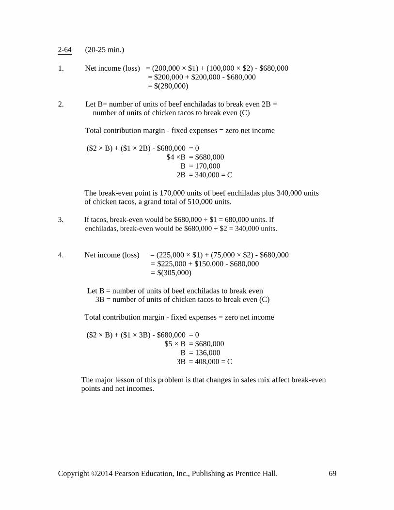
2-64 (20-25 min.)

1. Net income (loss) = (200,000 × $1) + (100,000 × $2) - $680,000

= $200,000 + $200,000 - $680,000

= $(280,000)

2. Let B= number of units of beef enchiladas to break even 2B = number of units of chicken tacos to break even (C)

Total contribution margin - fixed expenses = zero net income

($2 × B) + ($1 × 2B) - $680,000 = 0

$4 ×B = $680,000

B = 170,000

2B = 340,000 = C

The break-even point is 170,000 units of beef enchiladas plus 340,000 units of chicken tacos, a grand total of 510,000 units.

3. If tacos, break-even would be $680,000 ÷ $1 = 680,000 units. If

enchiladas, break-even would be $680,000 ÷ $2 = 340,000 units.

4. Net income (loss) = (225,000 × $1) + (75,000 × $2) - $680,000

= $225,000 + $150,000 - $680,000

= $(305,000)

Let B = number of units of beef enchiladas to break even 3B = number of units of chicken tacos to break even (C)

Total contribution margin - fixed expenses = zero net income

($2 × B) + ($1 × 3B) - $680,000 = 0

$5 × B = $680,000

B = 136,000

3B = 408,000 = C

The major lesson of this problem is that changes in sales mix affect break-even points and net incomes.


2-65 (20-25 min.)

1. Let S = number of self-pay patients (S)

3S = number of other patients (G)

($1,250 × S) + ($950 × 3S) – ($750 × S) – ($750 × 3S) - $52,800,000 = 0

($1,250 × S) + ($2,850 × S) – ($750 × S) – ($2,250 × S) = $52,800,000

$1,100 × S = $52,800,000

S = 48,000

3S = 144,000 = G

The break-even point is 48,000 self-pay patient days plus 48,000 × 3 = 144,000 other patient days, a grand total of 192,000 patient days.

2. Contribution margins: S = $1,250 - $750 = $500 per patient day G = $950 - $750 = $200 per patient day

Patient days: S = .40 × 172,000 = 68,800 G = .60 × 172,000 = 103,200

Net income = (68,800 × $500) + (103,200 × $200) - $52,800,000 =

$34,400,000 + $20,640,000 - $52,800,000 = $2,240,000

Let S = number of self-pay patients (S)

1.5S = number of other patients (G)

($1,250 × S) + ($950 ×1.5S) – ($750 × S) – ($750 ×1.5S) - $52,800,000 = 0

($1,250 × S) + ($1,425 × S) – ($750 × S) – ($1,125 × S) = $52,800,000

$800 × S = $52,800,000

S = 66,000

1.5S = 99,000 = G

The break-even point is now lower (66,000 + 99,000 = 165,000 patient days instead of 48,000 + 144,000 = 192,000 patient days).


2-66 (15-25 min.)

1. Let N = number of rooms

($90 × N) – ($42 × N) - $8,700,000 = $801,000

(1 - .25)

($48 × N) - $8,700,000 = $1,068,000

$48 ×N = $9,768,000

N = 203,500 rooms

($48 × N) - $8,700,000 = $400,500

(1 - .25)

($48 × N) - $8,700,000 = $534,000 $48 × N = $9,234,000

N = 192,375 rooms

2.($90 × N) – ($42 × N) - $8,700,000 = 0

$48 × N = $8,700,000

N = 181,250 rooms

Number of rooms at 100% capacity = 570 × 365 = 208,050 Percentage occupancy to break even = 181,250 ÷ 208,050 = 87.1%

3. Using the shortcut approach described in the chapter appendix:

Change in net income = Change in vol. in units × Cont. margin/unit × (1 - tax rate)

= 6,000 × $48 × (1 - .25)

= 6,000 × $36

= $216,000.

Note that a 3% increase in rooms rented increased net income by $216,000 ÷ $675,000 or 32%.

Rooms rented 200,000 206,000

Contribution margin @ $48 $9,600,000 $9,888,000 Fixed expenses 8,700,000 8,700,000

Income before taxes 900,000 1,188,000 Income taxes @ 25% 225,000 297,000 Net income $ 675,000 $ 891,000

Increase in net income $216,000

Percentage increase 32%


2-67 (15-25 min.)

Current contribution margin = $15 - $8 - $4 = $3.

New variable costs per disk will be (125% x $8 ) + $4 = $10 + $4 = $14.

1. Break-even point = $714,000 = 238,000 CDs

$15- ($8 + $4)

2. Contribution margin: $15 - ($8 + $4) = $3

Increased after-tax income after 15% increase in volume:

Change in net income = Increase in vol. in units × Cont. margin/unit × (1 - tax rate) = 25,500 × $3 × (1 - .40)

= $45,900 increase in income

3. Let N = target sales in units

25% increase in unit purchase price will increase purchase price to $10 (from previous value of $8) so variable costs per unit will be $10 + $4 = $14.

Target sales – Variable costs – Fixed costs = target after-tax net income

1 - tax rate

($15 × N) – ($14 × N) - $714,000 = $90,000 ÷ (1 - .4)

($15 × N) – ($14 × N) - $714,000 = $150,000

$1 × N = $864,000

N = 864,000 units

$15 × N = $12,960,000

4. Let P = new selling price

Current contribution ratio is $3 ÷ $15 = .20

New contribution ratio is (P - $14) ÷ P = .20

.20P = P - $14

.80P = $14

P = $14 ÷ .80

P = $17.5


2-68 (25-35 min.)

1. $12,150,000 ÷ $810 = 15,000 patient-days

2. Variable costs = $3,300,000 ÷ 15,000 = $220 per patient-day

Contribution margin = $810 - $220 = $590 per patient-day

To recoup the specified fixed expenses:

$5,900,000 ÷ $590 = 10,000 patient-days

3. The fixed cost levels differ as the relevant range changes:

Non-Nursing Nursing Total Patient-Days Fixed Expenses Fixed Expenses Fixed Expenses

10,000-12,000 $5,900,000 $1,350,000(a) $7,250,000

12,001-16,000 5,900,000 1,575,000(b) 7,475,000

(a) $45,000 × 30 = $1,350,000

(b) $45,000 × 35 = $1,575,000

To break even on a lower level of fixed costs:

$7,250,000 ÷ $590 = 12,288 patient-days

This answer exceeds the lower-level maximum; therefore, this answer is infeasible. The department must operate at a $7,475,000 level of fixed costs to break even: $7,475,000 ÷ $590 = 12,669 patient-days.

4. The nursing costs would have been variable instead of fixed. The contribution margin per patient-day would have been $810 - $220 - $200 = $390. The break-even point would be higher: $5,900,000 ÷ 390 = 15,128 patient-days.

Some instructors might want to point out that hospitals have been under severe pressures to reduce costs. More than ever, nursing costs are controlled

as variable rather than fixed costs. For example, more part-time help is used, and nurses may be used for full shifts but only as volume requires.


2-69 (15-20 min.)

1. Old: (Contribution margin × 600,000) - $580,000 = Budgeted profit [($3.10 - $2.10) × 600,000] - $580,000 = $20,000

New: (Contribution margin × 600,000) - $1,140,000 = Budgeted profit [($3.10 - 1.10) × 600,000] - $1,140,000 = $60,000

2. Old: $580,000 ÷ $1.00 = 580,000 units

New: $1,140,000 ÷ $2.00 = 570,000 units

3. A fall in volume will be more devastating under the new system because the high fixed costs will not be affected by the fall in volume:

Old: ($1.00 × 500,000) - $580,000 = –$80,000 (an $80,000 loss)

New: ($2.00 × 500,000) - $1,140,000 = –$140,000 (a $140,000 loss)

The 100,000 unit fall in volume caused a $20,000 - (- $80,000) = $100,000 decrease in profits in the old environment and a $60,000 - ( -

$140,000) = $200,000 decrease in the new environment.

4. Increases in volume create larger increases in profit in the new environment:

Old: ($1.00 × 700,000) - $580,000 = $120,000

New: ($2.00 × 700,000) - $1,140,000 = $260,000

The 100,000 unit increase in volume caused a $120,000 - $20,000 = $100,000 increase in profit under the old environment and a $260,000 - $60,000 = $200,000 increase under the new environment.

5. Changes in volume affect profits in the new environment (a high fixed cost,

low variable cost environment) more than they affect profits in the old

environment. Therefore, profits in the old environment are more stable and less

risky. The higher risk new environment promises greater rewards when

conditions are favorable, but also leads to greater losses when conditions are

unfavorable, a more risky situation.


2-70 (25-30 min.) This case is based on real data that has been simplified so that the numbers are easier to handle.

1. Daily break-even volume is 85 dinners and 170 lunches:

First compute contribution margins on lunches and dinners:

Variable cost percentage = ($1,246,500 + $222,380) ÷ $2,098,400

= 70% Contribution margin percentage = 1 - variable cost percentage

= 1 - 70% = 30%

Lunch contribution margin = .30 × $20 = $6

Dinner contribution margin = .30 × $40 = $12

Annual fixed cost is $170,940 + $451,500 = $622,440

Let X = number of dinners and 2X = number of lunches

($12×X) + ($6×2X) - $622,440 = 0

$24(X) = $622,440

X = 25,935 dinners annually to break even

2X = 51,870 lunches annually to break even

On a daily basis: Dinners to break even = 25,935 ÷ 305 = 85 dinners daily

Lunches to break even = 85 × 2 = 170 lunches daily or

51,870 ÷ 305 = 170 lunches daily.

To determine the actual volume, let Y be a combination of 1 dinner and 2

lunches. The price of Y is $40 + (2 × $20) = $80, and total volume in units of Y

is $2,098,400 ÷ $80 = 26,230 and daily volume is 26,230 ÷ 305 = 86. Therefore, 86 dinners and 2 × 86 = 172 lunches were served on an average day. This is 1

dinner and 2 lunches above the break-even volume.

2. The extra annual contribution margin from the 3 dinners and 6 lunches is:

3 × $40 × .30 × 305 = $10,980 + 6 × $20 × .30 × 305 = 10,980 Total $21,960

The added contribution margin is greater than the $15,000 advertising expenditure. Therefore, the advertising expenditure would be warranted. It would increase operating income by $21,960 - $15,000 = $6,960.


3. Let Y again be a combination of 1 dinner and 2 lunches, priced at $80. Variable

costs are .70 × $80 = $56, of which $56 × .25 = $14 is food cost. Cutting food

costs by 20% reduces variable costs by .20 × $14 = $2.80, making the variable

cost of Y $56 - $2.80 = $53.20 and the contribution margin $80 - $53.20 =

$26.80. (This could also be determined by adding the $2.80 saving in food cost

directly to the old contribution margin of $24.) The required annual volume in Y

needed to keep operating income at $7,080 is:

$26.80 (Y) - $622,440 = $7,080

$26.80 (Y) = $629,520

Y = 23,490

Therefore, daily volume = 23,490 ÷ 305 = 77 (rounded)

If volume drops no more than 86 - 77 = 9 dinners and 172 - 154 = 18 lunches,

using the less costly food is more profitable. However, there are many subjective

factors to be considered. Volume may not fall in the short run, but the decline in

quality may eventually affect repeat business and cause a long-run decline.

Much may depend on the skill of the chef. If the quality difference is not readily

noticeable, so that volume falls less than, say, 10%, saving money on the

purchases of food may be desirable.


2-71 (25-30 min.)

1. Break-even in pounds = Annual fixed costs ÷ Contribution margin/pound $566,250

= (5.00 - $3.00) = 283,125 pounds

2. Contribution margin ratio = $2.00 ÷ $5.00 = 40%

Old variable cost = $3.00

Only the cost of salmon is affected:

New variable cost = $3.00 + (.15 ×$2.50) = $3.375

Let S = Selling price

Selling price - Variable costs = Contribution margin

(S - $3.375) = .40S

.60S = $3.375

S = $5.625

Check: ($5.625 - $3.375) ÷ $5.625 = 40%

3. Current income before taxes:

= 390,000 × ($5.00 - $3.00) - $566,250

= $780,000 - $566,250 = $213,750

Current income after taxes:

= $213,750 × .60 = $128,250

The problem can be solved by using units and then converting to dollar sales.

Let N = sales in pounds

Sales - Variable expenses - Fixed expenses =

Net income

1 - tax rate

($5.00 × N) – {[($3.00 + .15×$2.50)] × N} - $566,250 =$128,250 ÷ (1 - .4)

($5.00 × N) – ($3.375 × N) - $566,250 = $213,750

$1.625 × N = $780,000

N = 480,000 pounds

$5.00 × N = $2,400,000 sales

An alternative way to get the solution is: New contribution margin ratio = ($5.00- $3.375) ÷ $5.00 = .325 New variable-cost ratio = 1.000 - .325 = .675

Let S = Sales

S = (.675 × S) + $566,250 + [$128,250 ÷ (1 - .4)] .325 × S = $780,000 S

= $2,400,000


4. Strategies might include:

(a) Increase selling price by the $.375 cost increase.

(b) Decrease other variable costs by $.375 per pound.

(c) Decrease fixed costs by $.375 × 390,000 = $146,250.

(d) Increase unit sales by 480,000 - 390,000 = 90,000 pounds.

(e) Some combination of the above.

2-72 (15-20 min.)

1. The following table shows the comparison between percentage changes in total revenue and income before taxes for the six major regions of Nike.

Percent Change Percent Change Region in Revenue in Pre-tax Income

North America 13% 14%

Western Europe –2% –16%

Central & Eastern Europe 4% –8%

Greater China 18% 22%

Japan –13% –37%

Emerging Markets 24% 32%

The term operating leverage means that a substantial portion of the resources

used to generate income were fixed-cost resources and did not increase in response to increased revenue-generating activities. As a result, income changes

more than proportional to the change in revenue.

2. There are many possible explanations. One possibility is that while revenues

increased, variable costs may have increased so that the overall contribution margin fell, resulting in a decrease in income. Another possibility is that even if

variable costs did not increase, fixed costs may have increased by an amount that more than offset the increased contribution from increased sales.

3. Nike’s operating leverage is the ratio of its fixed costs to variable costs. A large

percentage of Nike’s costs is cost of goods sold, which is primarily a variable cost, making operating leverage low. However, Nike also has many fixed costs. Many of Nike’s fixed costs are related to its distribution function. The costs of the distribution center, equipment, and salaries of regular employees and

management all contribute to a substantial fixed-cost component of total cost. Another significant component of fixed costs is the Nike World Campus in

Beaverton, Oregon with 16 buildings and almost 6,000 management staff.

2-73 (30-40 min.) For the solution to this Excel Application Exercise, follow the step-by-step instructions provided in the textbook chapter. Answers to the questions follow:

1. Proposal A:

Break even in units: $110,000 ÷ ($99 - $55) = 2,500 units

Break even in dollars: 2,500 × $99 = $247,500

Proposal B:




Proposal C:



2. The break-even points are much smaller because the contribution margin is larger while the fixed costs are unchanged.

3. The increase in contribution margin was not nearly as large, $6 in proposal

C compared to $30 in proposal B.

2-74 (30 min. or more) The purpose of this problem is to develop an intuitive feel for the costs

involved in a simple production process and to assess whether various costs are fixed or variable. Then students must assess the market to determine a price so that they can compute a break-even point.

Completing this problem can be done quickly or it can take much time. It might

even be done in class, with students suggesting the various costs and predicting their

levels. A complete analysis might involve finding the actual prices of the resources

needed to make the product or service. This could lead to time-consuming research.

Whatever approach is taken, students are led to see the real-world application of what

they are learning.


2-75 (30-40 min.) NOTE TO INSTRUCTOR: This solution is based on the web site as it was in early 2012. Be sure to examine the current web site before assigning this problem, as the information there may have changed.

1. Answers to the questions depend on the student's location and choices of dates.

Fares available include business select, anytime, and “wanna get away”. Different

fares are offered because of the different costs incurred by SWA to serve

customers who have different flying needs. Another factor causing different fares

is the need to match products offered by competing airlines. Restrictions such as

the requirement to make reservations at least 7 days in advance of travel are

necessary to give SWA planning information in advance. Limiting the number of

reduced-price wanna get away fares on each flight is necessary in order to keep

open seats for customers who must travel on short notice.

2. It is likely that the fares one week in advance are higher than the fares one month in advance. Customers who need to travel with short notice are willing to pay more. Many business travelers fly with very short notice.

3. On a particular flight, price paid for a seat (assuming the same class seat) is not a

cost driver. The various costs incurred by SWA will change only slightly – possibly the type of food served will vary as a function of the price paid for a seat

on a particular trip, but almost all the other costs are independent of the price paid for the seat.

4. Operating revenues and operating expenses are reported for the current and prior

year along with the percentage change. The operating revenues increased from

$12.104 billion in 2010 to $15.658 billion in 2011, an increase of 29.4%.

Operating expenses increased from $11.116 billion in 2011 to $14.965 billion in

2011, an increase of 34.6%. With expenses rising faster than revenues, profits

will fall – as shown by the 29.8% decrease in operating income.

5. To describe a particular cost as fixed or variable, we must identify the cost

driver, the time period involved, and the relevant range. In this case, assume that the period is one year and the relevant range is the number of ASMs that can be

available without adding to or subtracting from the current fleet of airplanes. Thus, adding ASMs means flying the existing airplanes for more hours.

Costs that would probably vary with ASMs are salaries, wages, and benefits, employee retirement plans, fuel and oil, maintenance materials and repairs,

landing fees and other rentals. Aircraft rentals and depreciation would probably be

fixed costs.

Some of these costs might be more directly caused by other cost drivers. For example, revenue passenger miles (RPM), that is number of passengers times the

miles each flies, might drive agency commissions and possibly some salaries (for

example, flight attendants whose number depends on how many passengers are on a particular flight).


introduction to management accounting 16th edition by charles t. horngren… · 2018-09-20 · 2-b1...

Documents