Introduction to Machine Learning

CMU-10701Markov Chain Monte Carlo Methods

Barnabás Póczos & Aarti Singh

2

Contents

� Markov Chain Monte Carlo Methods

• Goal & Motivation

� Sampling

• Rejection

• Importance

� Markov Chains

• Properties

� MCMC sampling

• Hastings-Metropolis

• Gibbs

3

Monte Carlo Methods

4

� A recent survey places the Metropolis algorithm among the

10 algorithms that have had the greatest influence on the development and practice of science and engineering in the 20th

century (Beichl&Sullivan, 2000).

� The Metropolis algorithm is an instance of a large class of sampling algorithms, known as Markov chain Monte Carlo (MCMC).

The importance of MCMC

5

� Bayesian inference and learning

� Normalization

� Marginalization

� Expectation

� Sampling from high-dimensional, complicated distributions

� Global optimization

MCMC ApplicationsMCMC plays significant role in statistics, econometrics, physics and

computing science.

6

� The idea of Monte Carlo simulation is to draw an i.i.d. set of samples{x(i) } from a target density p(x) defined on a high-dim. space X.

The Monte Carlo principle

� Our goal is to estimate the following integral:

Estimator:

7

Theorems

The Monte Carlo principle

Unbiased estimation

Independent of dimension d!

Asymptotically normal

a.s. consistent

8

� Monte Carlo methods need sample from distribution p(x).

� When p(x) has standard form, e.g. Uniform or Gaussian, it is straightforward to sample from it using easily available routines.

� However, when this is not the case, we need to introduce more sophisticated sampling techniques. ⇒ MCMC sampling

The Monte Carlo principle

One “tiny” problem…

9

Sampling

� Rejection sampling

� Importance sampling

10

Main Goal

Sample from distribution p(x) that is only known up to a proportionality constant

For example,

p(x) ∝ 0.3 exp(−0.2x2) +0.7 exp(−0.2(x − 10)2)

11

Rejection Sampling

12

Rejection Sampling Conditions

� p(x) is known up to a proportionality constant

p(x) ∝ 0.3 exp(−0.2x2) +0.7 exp(−0.2(x − 10)2)

� It is easy to sample from q(x) that satisfies p(x) ≤ M q(x), M < ∞

� M is known

Suppose that

13

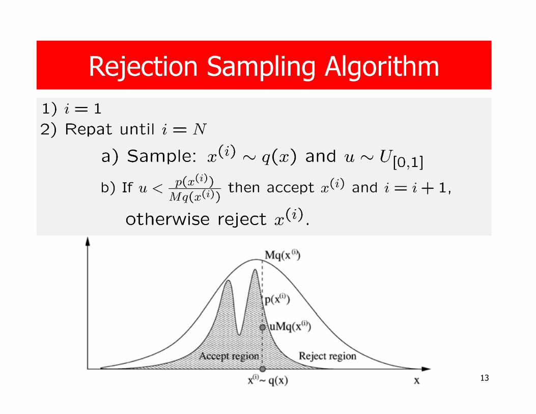
Rejection Sampling Algorithm

14

Rejection Sampling

The accepted x(i ) can be shown to be sampled with probability p(x) (Robert & Casella, 1999, p. 49).

Theorem

Severe limitations:

� It is not always possible to bound p(x)/q(x) with a reasonable constant M over the whole space X.

� If M is too large, the acceptance probability is too small.

� In high dimensional spaces it can be exponentially slow to sample points. (The points usually will be rejected)

15

Importance Sampling

16

Importance Sampling

� Importance sampling is an alternative “classical” solution that goes back to the 1940’s.

� Let us introduce, again, an arbitrary importance proposal distribution q(x) such that its support includes the support of p(x).

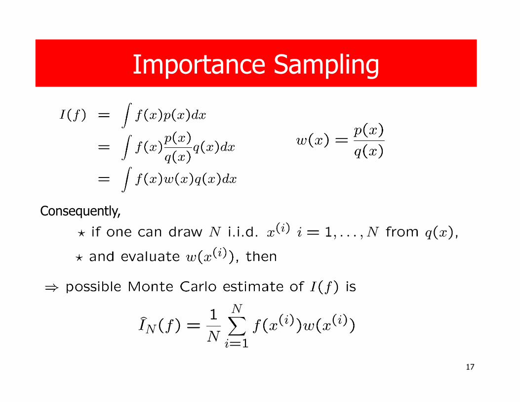
� Then we can rewrite I(f) as follows:

Goal: Sample from distribution p(x) that is only known up to a proportionality constant

17

Importance Sampling

Consequently,

18

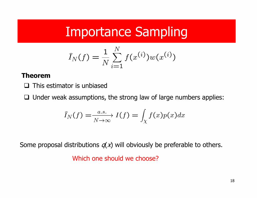
Importance Sampling

� This estimator is unbiased

� Under weak assumptions, the strong law of large numbers applies:

Some proposal distributions q(x) will obviously be preferable to others.

Theorem

Which one should we choose?

19

Importance Sampling

� This estimator is unbiased

� Under weak assumptions, the strong law of large numbers applies:

Some proposal distributions q(x) will obviously be preferable to others.

Theorem

20

Importance Sampling

The variance is minimal when we adopt the followingoptimal importance distribution:

Theorem

Find one that minimizes the variance of the estimator!

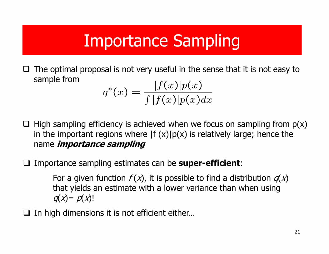
21

� Importance sampling estimates can be super-efficient:

For a given function f (x), it is possible to find a distribution q(x) that yields an estimate with a lower variance than when using q(x)= p(x)!

� In high dimensions it is not efficient either…

Importance Sampling

� The optimal proposal is not very useful in the sense that it is not easy to sample from

� High sampling efficiency is achieved when we focus on sampling from p(x) in the important regions where |f (x)|p(x) is relatively large; hence the name importance sampling

22

MCMC sampling - Main ideas

Create a Markov chain, which has the desired limiting distribution!

23

Markov Chains

Andrey Markov

24

Markov Chains

Markov chain:

Homogen Markov chain:

25

Markov Chains

� 1-Step state transition matrix:

� t-Step state transition matrix:

Lemma:

� Assume that the state space is finite:

Lemma: The state transition matrix is stochastic:

26

Markov chain with three states (s = 3)

Markov Chains Example

Transition graphTransition matrix

27

Definition:

[stationary distribution, invariant distribution, steady state distributions]

Markov Chains, stationary distribution

The stationary distribution might be not unique (e.g. T= identity matrix)

28

Markov Chains, limit distributions

If the probability vector for the initial state is

it follows that

and, after several iterations (multiplications by T )

no matter what initial distribution µ(x1) was.

limit distribution

The chain has forgotten its past.

Some Markov chains have unique limit distribution:

29

Our goal is to find conditions under which the Markov chain

converges to a unique limit distribution (independently from its starting state distribution)

Markov Chains

Observation:

If this limiting distribution exists, it has to be the stationary distribution.

30

Limit Theorem of Markov Chains

If the Markov chain is Irreducible and Aperiodic, then:

Theorem:

That is, the chain will convergence to the unique stationary distribution

31

For each pairs of states (i,j), there is a positive probability, starting in state i, that the process will ever enter state j.

= The matrix T cannot be reduced to separate smaller matrices

= Transition graph is connected.

Markov Chains

Definition

Irreducibility:

It is possible to get to any state from any state.

32

Markov Chains

Definition

The chain cannot get trapped in cycles.Aperiodicity:

A state i has period k if any return to state i, must occur in multiples of k time steps. Formally, the period of a state i is defined as

For example, suppose it is possible to return to the state in {6,8,10,12,...} time steps. Then k=2

(where "gcd" is the greatest common divisor)

Definition

33

Markov Chains

In other words,

a state i is aperiodic if there exists n such that for all n' ≥ n,

A Markov chain is aperiodic if every state is aperiodic.

Definition

Definition

The chain cannot get trapped in cycles.Aperiodicity:

34

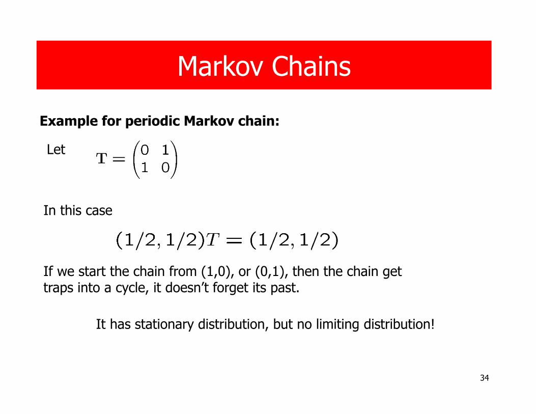
Let

If we start the chain from (1,0), or (0,1), then the chain get traps into a cycle, it doesn’t forget its past.

Markov Chains

Example for periodic Markov chain:

In this case

It has stationary distribution, but no limiting distribution!

35

A sufficient, but not necessary, condition to ensure that a particular π is

the desired invariant distribution of the Markov chain is the detailed balance condition.

Reversible Markov chains(Detailed Balance Property)

Definition: reversibility /detailed balance condition:

Theorem:

How can we find the limiting distribution of an irreducible and aperiodic Markov chain?

36

How fast can Markov chains forget the past?

� irreducible and aperiodic Markov chains

� have the target distribution as the invariant distribution.

� the detailed balance condition is satisfied.

It is also important to design samplers that converge quickly.

MCMC samplers are

37

� π is the left eigenvector of the matrix T with eigenvalue 1.

� The Perron-Frobenius theorem from linear algebra tells us that the remaining eigenvalues have absolute value less than 1.

� The second largest eigenvalue, therefore, determines the rate of convergence of the chain, and should be as small as possible.

Spectral properties

Theorem: If

38

The Hastings-Metropolis Algorithm

39

The Hastings-Metropolis Algorithm

Our goal:

The main idea is to construct a time-reversible Markov chain with (π,…,πm) limit distributions

We don’t know B !

Generate samples from the following discrete distribution:

Later we will discuss what to do when the distribution is continuous

40

The Hastings-Metropolis Algorithm

Let {1,2,…,m} be the state space of a Markov chain that we can simulate.

No rejection: we use all X1, X2,… Xn, …

41

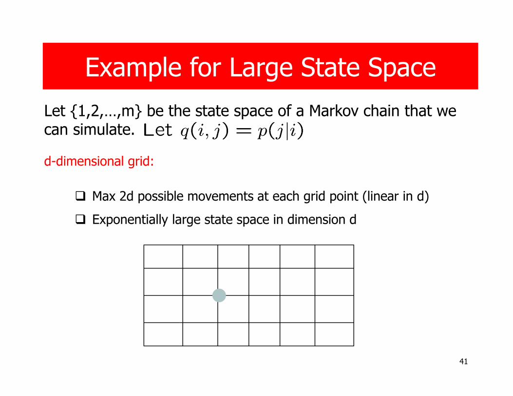
Example for Large State Space

Let {1,2,…,m} be the state space of a Markov chain that we can simulate.

d-dimensional grid:

� Max 2d possible movements at each grid point (linear in d)

� Exponentially large state space in dimension d

42

The Hastings-Metropolis Algorithm

Theorem

Proof

43

The Hastings-Metropolis Algorithm

Observation

Corollary

Theorem

Proof:

44

The Hastings-Metropolis Algorithm

Proof:

Theorem

Note:

45

The Hastings-Metropolis Algorithm

It is not rejection sampling, we use all the samples!

46

Continuous Distributions

� The same algorithm can be used for continuous distributions as well.

� In this case, the state space is continuous.

47q(x | x(i )) = N(x(i), 100), 5000 iterations

Bimodal target distribution: p(x) ∝ 0.3 exp(−0.2x2) +0.7 exp(−0.2(x − 10)2)

Experiment with HM

An application for continuous distributions

48

Good proposal distrib. is important

49

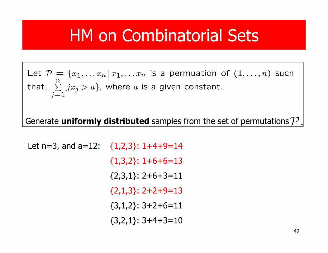
HM on Combinatorial Sets

Generate uniformly distributed samples from the set of permutations

{1,2,3}: 1+4+9=14

{1,3,2}: 1+6+6=13

{2,3,1}: 2+6+3=11

{2,1,3}: 2+2+9=13

{3,1,2}: 3+2+6=11

{3,2,1}: 3+4+3=10

Let n=3, and a=12:

50

To define a simple Markov chain on , we need the concept of

neighboring elements (permutations):

Definition: Two permutations are neighbors, if one results from the interchange of two of the positions of the other:

(1,2,3,4) and (1,2,4,3) are neighbors.

(1,2,3,4) and (1,3,4,2) are not neighbors.

HM on Combinatorial Sets

51

HM on Combinatorial Sets

That is what we wanted!

52

Gibbs Sampling: The Problem

Our goal is to generate samples from

Suppose that we can generate samples from

53

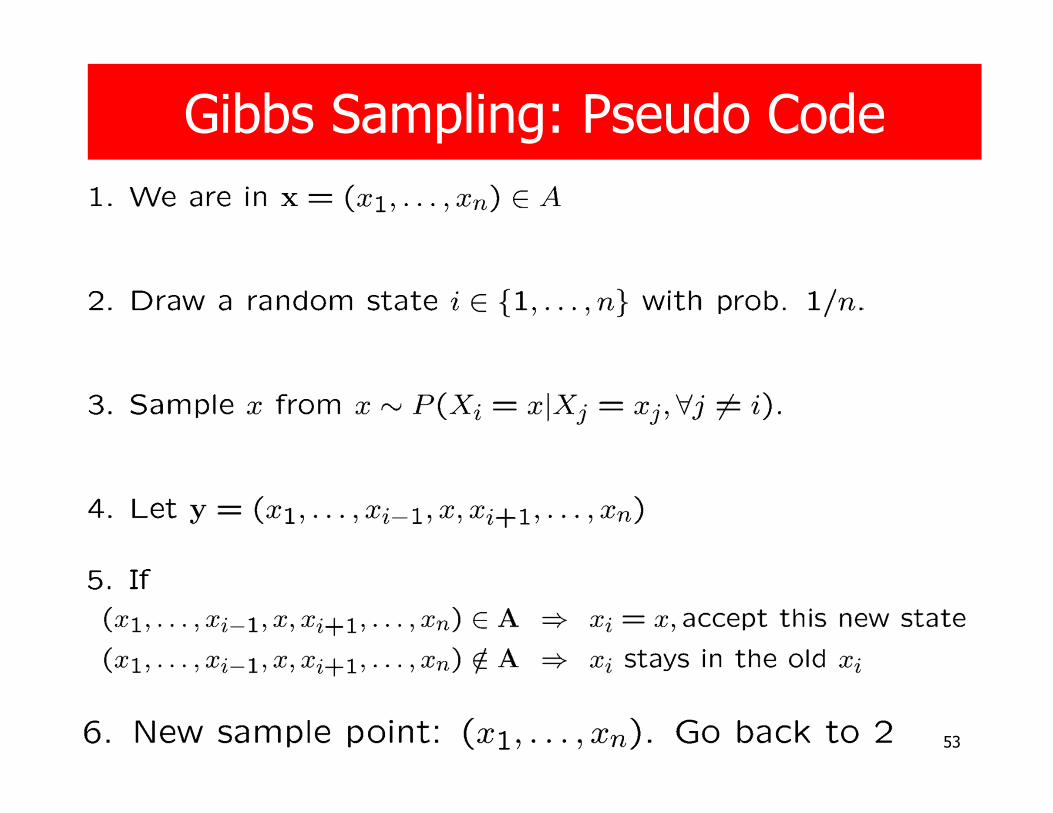
Gibbs Sampling: Pseudo Code

54

Gibbs Sampling: Theory

Let

and let

Observation: By construction, this HM sampler would sample from

Consider the following HM sampler:

We will prove that this HM sampler = Gibbs sampler.

55

Gibbs Sampling is a Special HM

Proof:

By definition:

Theorem: The Gibbs sampling is a special case of HM with

56

Gibbs Sampling is a Special HM

Proof:

57

Gibbs Sampling in Practice

58

Simulated Annealing

59

Goal: Find

Simulated Annealing

60

Theorem:

Proof:

Simulated Annealing

61

Main idea

Simulated Annealing

� Let λ be big.

� Generate a Markov chain with limit distribution Pλ(x).

� In long run, the Markov chain will jump among the maximum points of Pλ(x).

Introduce the relationship of neighboring vectors:

62

Uniform distribution

Use the Hastings- Metropolis sampling:

Simulated Annealing

63

With prob. α accept the new state

with prob. (1-α) don't accept and stay

Simulated Annealing: Pseudo Code

64

With prob. α=1 accept the new state since

we increased V

Simulated Annealing: Special case

In this special case:

65

Simulated Annealing: Problems

66

Simulated Annealing

Temperature = 1/ λ

67

Simulated Annealing

68

Monte Carlo EM

E Step:

Monte Carlo EM:

Then the integral can be approximated! ☺☺☺☺

69

Monte Carlo EM

70

Thanks for the Attention! ☺