introduction to kinetic models for biomass pyrolysis....

1

Introduction to kinetic models for biomass pyrolysis. Part 1.

Gábor VárhegyiInstitute of Materials & Environmental Chemistry

Chemical Research CenterHungarian Academy of Sciences

2

What we can overview during 2×50 minutes? Pyrolysis is the 1st of the three main steps of combustion. It

also has roles in other industrial processes. Pyrolysis modeling is a huge area, however. It includes kinetics, transport processes, product distributions, effects of the mineral matter (as catalysts), effect of the volatile products when their escape is hindered (in close reactors), and so on ...

Due to our limited time, we shall restrict the treatment for the kinetic part only. Besides we shall treat kinetic models with only a limited number of kinetic equations.

We shall deal with thermal analysis experiments when the kinetic regime can be well ensured. Mainly TGA.

3

Definitions:

Definition of thermal analysis: A sample is subjected to a T(t) temperature program and one or more quantities are measured as function of time or temperature mass, heat flux, mass spectrometric intensities, etc. every sort of time-resolved pyrolysis experiments

Definition of kinetics: The study of the rate(s) of change(s) in a physical or chemical system

Definition of kinetic control: When transport processes do not alter the rate(s) of change(s) significantly

4

Is thermal analysis a marginal topic? Estimations from the 2005 data of the Science Citation Index:

ca. 10 000 papers mentions a thermal analysis technique in title, abstract, or keywords in a year

ca. 2 000 papers are based mainly on thermal analysis in a year

ca. 25% of the latter group deals with kinetics on some level

Why we need kinetics in thermal analysis? Not for activation energies or preexponential factors!

5

Why Thermal Analysis? (Why not something else?) A problem: During a combustion the heating of the fuel is

usually very fast. Even tobacco smoothing implies a 30°C/second heating of the tobacco grains. On the other hand, a typical safe heating rate in thermal analysis is 40°C/minute. When the reaction heat does not cause problems, we can go up till ca. 100°C/min.

Are there other techniques that can measure higher heating rates with a high precision in the kinetic regime? If the sample is in flame, for example, then we have only rough estimation on its true temperature. Besides, the mass measurement has a higher precision than anything else. But we cannot measure the sample mass accurately if a particle burns in a split second.

6

What limits the heating rate in TGA? (A qualitative reasoning) If we heat something fast, it will not

have time to react at lower temperatures. So the reaction occurs at higher temperatures where the reaction rate is obviously higher. Later we shall see (by simple mathematical deductions as well as on actual experiments) that the reaction rate is nearly proportional with the heating rate.

In a TGA experiment the sample mass should be at least 0.1 – 0.5 mg, depending on the sensitivity and stability of the apparatus. Usually we put a few grains or a thin layer into a sample plan of ca. ∅ 6 mm.

Heat production is proportional to reaction rate ⇒ ignition (strong self-heating or even flames).

So does heat consumption (pyrolysis in inert gas) ⇒ self cooling

7Temperature [°C]

-dm

/dt

[s-1]

× 1

03

400 450 500 550 600

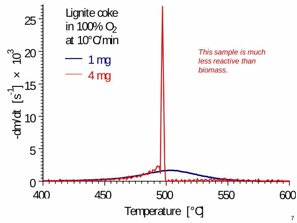
Lignite cokein 100% O2at 10°C/min

1 mg 4 mg

0

5

10

15

20

25

This sample is much less reactive than biomass.

8

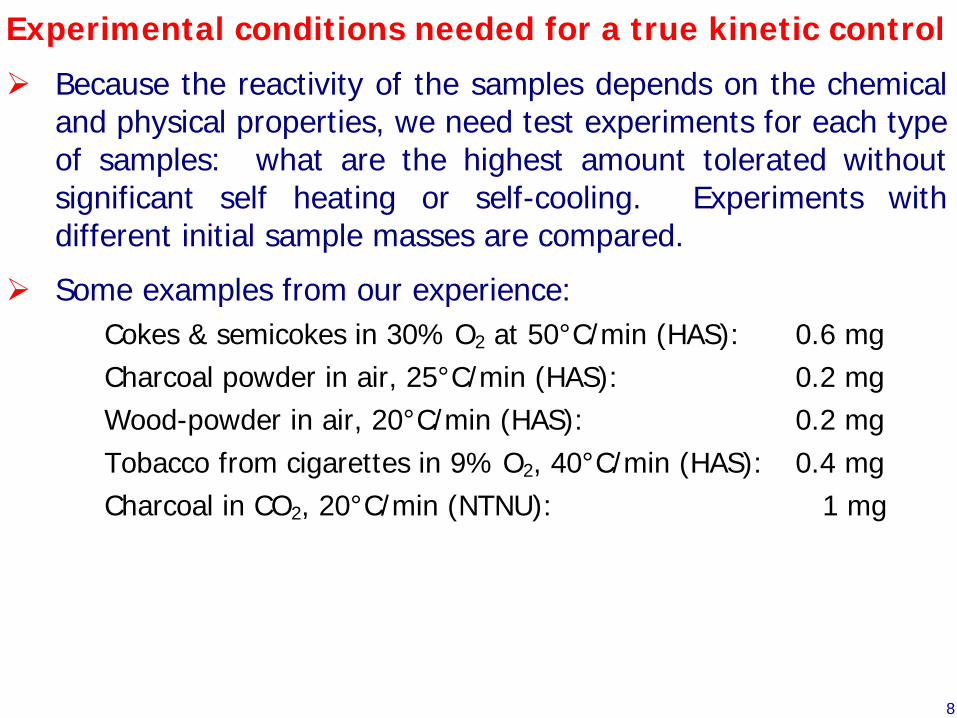
Experimental conditions needed for a true kinetic control

Because the reactivity of the samples depends on the chemical and physical properties, we need test experiments for each type of samples: what are the highest amount tolerated without significant self heating or self-cooling. Experiments with different initial sample masses are compared.

Some examples from our experience: Cokes & semicokes in 30% O2 at 50°C/min (HAS): 0.6 mg Charcoal powder in air, 25°C/min (HAS): 0.2 mg Wood-powder in air, 20°C/min (HAS): 0.2 mg Tobacco from cigarettes in 9% O2, 40°C/min (HAS): 0.4 mg Charcoal in CO2, 20°C/min (NTNU): 1 mg

9

Experimental conditions needed for a true kinetic control

It is easier in pyrolysis studies, when the reaction is endothermic and the reaction heat has smaller magnitudes. If it is small and the sample has a loose structure, then the sample mass at 40°C/min can be as much as 20 mg as shown by Mette Stenseng, Anker Jensen and Kim Dam-Johansen for straws. Which is a rare and lucky situation. It’s advisable to carry out a few test experiments at each new type of samples in the given apparatus.

10

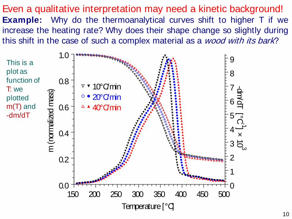
Even a qualitative interpretation may need a kinetic background! Example: Why do the thermoanalytical curves shift to higher T if we increase the heating rate? Why does their shape change so slightly during this shift in the case of such a complex material as a wood with its bark?

Temperature [°C]

m (n

orm

alize

d m

ass)

-dm/dT [°C

-1] × 10 3

10°C/min 20°C/min 40°C/min

150 200 250 300 350 400 450 5000.0

0.2

0.4

0.6

0.8

1.0

0

1

2

3

4

5

6

7

8

9

This is a plot as function of T: we plotted m(T) and-dm/dT

11

What quantitative characteristics can be obtained without a kinetic model? Examples:

Temperature [°C]

m (n

orm

alize

d m

ass) -dm

/dt [s -1] × 10 3

m500°C

(-dm/dt)peak

Thc.onset Tpeak Toffset 5000.0

0.2

0.4

0.6

0.8

1.0

0.0

0.5

1.0

1.5

12

T (°C)200 300 400

0.0

0.1

0.2

-dm/dt(%/s)

Extractives, hemicellulose,

lignin

HemicelluloseCellulose

Lignin

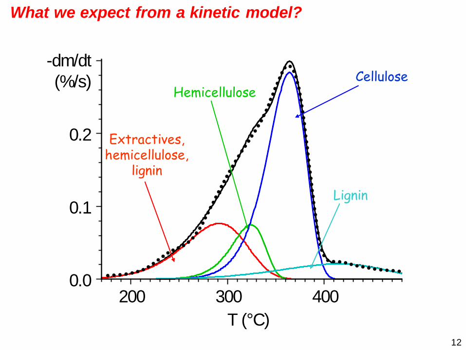
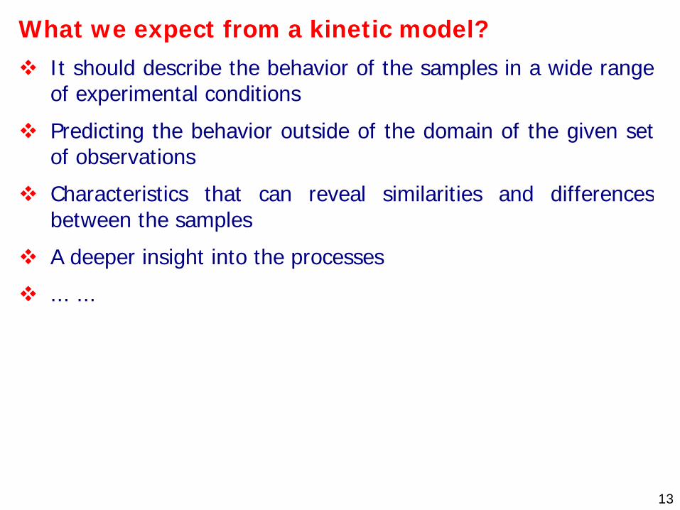
What we expect from a kinetic model?

13

What we expect from a kinetic model? It should describe the behavior of the samples in a wide range

of experimental conditions

Predicting the behavior outside of the domain of the given set of observations

Characteristics that can reveal similarities and differences between the samples

A deeper insight into the processes

... ...

14

Three reaction types. 1. First order reactions We can use this approximation to describe the decomposition of either a sample or a part of the sample.

Whatever we describe with it, let us denote its reacted fraction by α(t):

α(0)=0 and α(∞)=1

The fraction available for reaction in a given moment is 1-α(t).

The reaction rate, dα/dt obviously depends on 1-α(t). The simplest approximation:

dα/dt ≅ A e–E/RT [1-α(t)]

Let us separate the variables and integrate the equation:

''1

'

0

)'(/

0

dteAd ttRTE∫∫ −=

−

α

αα

or ')(

0

)'(/ dteAgt

tRTE∫ −=α

15260 280 300 320 340 360 380 °C

0.00

0.25

0.50

0.75

1.00

1.25

-dm/dt%/s

We have 3 unknown parameters for this peak:

E (kJ/mol)

A (s-1)

c the area beneath thecurve

1st order kinetics at a constant heating rate [linear T(t)]

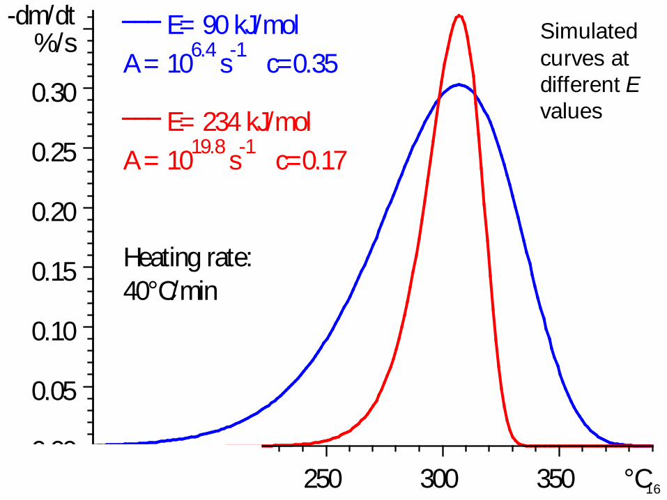
16150 200 250 300 350 °C

E= 90 kJ/molA = 106.4 s-1 c=0.35

E= 234 kJ/molA = 1019.8 s-1 c=0.17

Heating rate:40°C/min

0.00

0.05

0.10

0.15

0.20

0.25

0.30

-dm/dt%/s Simulated

curves at different Evalues

17

Three reaction types. 2. A more general type of reactions α(0)=0, α(∞)=1, fraction available for reaction: 1-α(t).

There are effects that can alter the kinetics from the first order behavior. E.g. differences between the reacting species. Or the growth of the reaction surface during car burn-off or char gasification:

dα/dt ≅ A e–E/RT f(α)

where f(α) is an empirical function

Let us separate the variables and integrate the equation:

')'(

'

0

)'(/

0

dteAfd t

tRTE∫∫ −=α

αα

or ')(

0

)'(/ dteAgt

tRTE∫ −=α

18

Kinetic equation: dα/dt = A exp(–E/RT) f(α)

α (reacted fraction)

f( α) s

caled

to u

nity

0.0 0.1 0.2 0.3 0.4 0.5 0.6 0.7 0.8 0.9 1.0

1st order nucleation (Avrami-Erofeev-Mampel) Randome pore theory (Su - Perlmutter) Contracting sphere 1st order kinetics 2-dimensional diffusion 3-dimensional diffusion

(Ginstling - Brounshtein) 3-dimensional diffusion

(Jander)

Examples for theoretically derived f(α) functions:

19

f 2(α 2

)

0.0 0.1 0.2 0.3 0.4 0.5 0.6 0.7 0.8 0.9 1.0

(a)f2(α2) of samples Top/11µm

Mid/11µmBot/11µmDem

0.0

0.1

0.2

0.3

0.4

0.5

0.6

0.7

0.8

0.9

1.0

f 3(α 3

)

0.0 0.1 0.2 0.3 0.4 0.5 0.6 0.7 0.8 0.9 1.0

(b)f3(α3) of samples Top/11µm

Mid/11µmBot/11µmDem

0.0

0.1

0.2

0.3

0.4

0.5

0.6

0.7

0.8

0.9

1.0

Empirical f(α) functions from a charcoal combustion study(Várhegyi et al, Ind. Eng. Chem. Res 2006)

f(α) ≅ const (α +z)a(1- α)n where a, n and z are parameters. This function can also describe reactions that accelerate at isothermal conditions.

Tomorrow we shall use only the rightmost part of this formula:

f(α) ≅ (1- α)n where n is the reaction order: any number between 0 andan upper limit chosen by us.

Name of the (1- α)n approximation: Power-law kinetics or n-order kinetics

20

Empirical f(α) functions from a charcoal gasification study

α3

f 3(α 3

)

+ + + + Birch, f(α)=(α+0.07)0.07 (1-α)0.47 / 0.99

Birch, f(α)=(1-α)0.44

- - - Pine, f(α)=(1-α)0.74

Shrinking core model, f(α)=(1-α)2/3

0.0 0.2 0.4 0.6 0.8 1.00.0

0.1

0.2

0.3

0.4

0.5

0.6

0.7

0.8

0.9

1.0 (Khalil et al, Energy & Fuels 2009)

21150 200 250 300 350 400 °C

n=0.5E= 68 kJ/mol

n=1E= 90 kJ/mol

n=3E= 150 kJ/mol

Heating rate:40°C/min

0.00

0.05

0.10

0.15

0.20

0.25

-dm/dt%/s Simulated

curves at different n values

22

The Coats – Redfern linearization from 1964

')(0

)'(/ dteAgt

tRTE∫ −=α where ')'(

')(0

αααα

α

dfdg ∫=

TRTE

EARg ln2ln)(ln +−≅β

α

where β is the heating rate in K/s.

It shows why the DTG curves are similar at different heating rates (β) when plotted as function of T. Example: Let us define a width as the T difference between the points α=2/3 and α=1/3 and let us neglect the slow change of the last term, 2 ln T. Then we have:

3/13/2

)3/1(ln)3/2(lnRT

ERT

Egg +−≈−

On a 1/T scale the width (1/T2/3-1/T1/3) is independent of β in this approximation. On a T scale it is not so, but the change of T2/3-T1/3 is not big.

Typical T values in biomass TGA: Tpeak ≈ 500 – 800 K, and its shift by a 10× increase of β is around 30K.

23

Distributed activation energy model (DAEM) Biomasses usually have very complex chemical and physical structure. A further complication comes from the mineral matter. So we have a wide range of species differing in reactivity. In DAEM the different reactivity of the species are described by different E. Let us look for those species that have a given E value in this model and let us apply a first order kinetics for their behavior. Let α(t,E) be their reacted fraction: α(0,E)=0 and α(∞,E)=1.

dα(t,E)/dt = A e-E/RT [1-α(t,E)] The overall reacted fraction, α(t) is the integral of α(t,E) terms taking into account that the different E values occur with different frequency:

∞

α(t) = ∫ D(E) α(t,E) dE 0 Here D(E) is a density function. Usually it is approximated by a Gaussian:

D(E) = (2π)-1/2 σ-1 exp[-(E-E0)2/2σ2]

24

Activation energy [kJ/mol]

Gau

ssia

n di

strib

utio

n

120 140 160 180 200 220 240 260 280

Numerical integration by E at a normal distribution:

Blue lines indicate the points where we actually solve the 1st order kineticequations in a numerical integration by a Gauss – Hermite quadrature. Iuse 150 quadrature points.

25200 250 300 350 400200 250 300 350 400200 250 300 350 400 °C

σ=0E= 90 kJ/mol

σ=12E= 234 kJ/mol

σ=20E= 368 kJ/mol

0.00

0.05

0.10

0.15

0.20

0.25

-dm/dt%/s

Reaction rates at different σ values at a linear T(t) (This curves approximate the same experimental data)

There are 4 parameters:E0, A, σ, and c.

Compensation effect!

26

T (°C)200 300 400

0.0

0.1

0.2

-dm/dt(%/s)


lignin


Lignin

Multicomponent models: An example of simple, 1st order partial reactions.

27

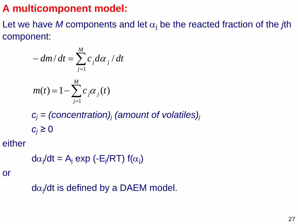
A multicomponent model: Let we have M components and let αj be the reacted fraction of the jth component:

∑=

=−M

jjj dtdcdtdm

1// α

∑=

−=M

jjj tctm

1)(1)( α

cj = (concentration)j (amount of volatiles)j cj ≥ 0

either dαj/dt = Aj exp (-Ej/RT) f(αj)

or dαj/dt is defined by a DAEM model.

28

The method of the least squares: ( ) ( )[ ] min

2

1 12 =

−=∑∑

= =

N

k

N

i kk

icalcki

obsk

N

k

hNtXtXS

Why? A good model describe the experimental data in a wide range of

experimental conditions We do not know yet other general criteria for the goodness of a

model *

Accordingly, we should prefer evaluation techniques that directly aim at this criterion

The evaluation of a large series of experiments by the method of least squares is a straightforward tool for this purpose.

A measure of the fit quality on a group of N experiments:

fitN (%) = 100 SN0.5

* The laws of the mathematical statistics do no offer help since the most important experimental errors are not random in thermal analysis.

29

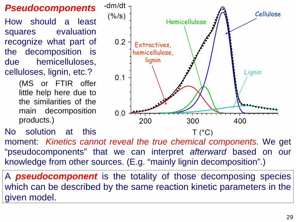
Pseudocomponents How should a least squares evaluation recognize what part of the decomposition is due hemicelluloses, celluloses, lignin, etc.?

(MS or FTIR offer little help here due to the similarities of the main decomposition products.)

No solution at this moment: Kinetics cannot reveal the true chemical components. We get “pseudocomponents” that we can interpret afterward based on our knowledge from other sources. (E.g. “mainly lignin decomposition”.)

A pseudocomponent is the totality of those decomposing species which can be described by the same reaction kinetic parameters in the given model.


lignin


Lignin


lignin


Lignin

30

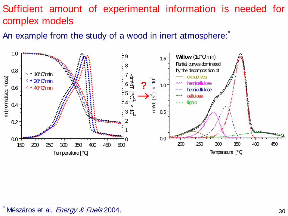
Sufficient amount of experimental information is needed for complex models An example from the study of a wood in inert atmosphere:*

Temperature [°C]

m (n

orm

alize

d m

ass)

-dm/dT [°C

-1] × 10 3


150 200 250 300 350 400 450 5000.0

0.2

0.4

0.6

0.8

1.0

0

1

2

3

4

5

6

7

8

9

? →

Temperature [°C]-d

m/d

t [s

-1]

× 1

03

Willow (10°C/min)Partial curves dominatedby the decomposition of

extractiveshemicellulose

hemicellulosecellulose

- - - lignin

200 250 300 350 400 4500.0

0.5

1.0

1.5

* Mészáros et al, Energy & Fuels 2004.

31

Sufficient amount of experimental information is needed for complex models (continued from the previous page)

Time [min]

Tem

pera

ture

[°C]

+ + + dT/dt = 40°C/mindT/dt = 20°C/min

- - - dT/dt = 10°C/min• • • • Stepwise T(t)

0 20 40 60 80 100 120 140 160 18050

100

150

200

250

300

350

400

450

→

Time [min]-d

m/d

t [s

-1]

× 1

03

Tem

pera

ture

[°C

]

Willowstepwise T(t)

0 20 40 60 80 100 120 140 160 1800.0

0.2

0.4

0.6

0.8

50

100

150

200

250

300

32

Examples from this work:M. Becidan, G. Várhegyi, J. E. Hustad, Ø. Skreiberg: Thermal decomposition of biomass wastes. A kinetic study. Ind. Eng. Chem. Res. 46 (2007) 2428-2437

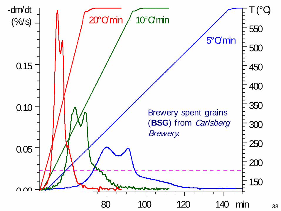
3360 80 100 120 140 min

5°C/min

10°C/min20°C/min

0.00

0.05

0.10

0.15

-dm/dt(%/s)

150

200

250

300

350

400

450

500

550

T (°C)

Brewery spent grains (BSG) from Carlsberg Brewery.

34200 300 400 500 °C

0.000

0.005

0.010

0.015

-dm/dt(%/s)

150

200

250

300

350

400

450

500

550

T (°C)

A “constant reaction rate” (CRR) experiment on the Carlsberg residue (BSG) sample

35Time (min)

Tem

pera

ture

(°C

)

0 50 100 150 200


CRR stepwise

150

200

250

300

350

400

450

500

550

600

5 different temperature programs were used

36Time [min]

-dm

/dt

[s-1]

× 1

03 Temperature [°C]

0 10 20 30 40

BSGT(t): 20°C/minFit: 2.0%

0.00.20.40.60.81.01.21.41.61.82.0

200

300

400

500

600

3 DAEM reactions,3×4=12 unknown parameters (Aj, E0,j, σj

and cj, j=1,2,3).

37Time [min]

-dm

/dt

[s-1]

× 1


0 20 40 60 80

BSGT(t): CRRFit: 3.0%

0.0

0.2

200

300

400

500

38Time [min]

-dm

/dt

[s-1]

× 1


0 50 100 150 200

BSGT(t): stepwiseFit: 1.4%

0.0

0.2

0.4

0.6

200

300

400

500

600

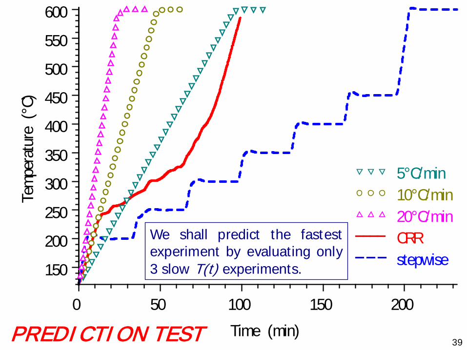
39Time (min)

Tem

pera

ture

(°C

)

0 50 100 150 200


CRR stepwise

150

200

250

300

350

400

450

500

550

600

We shall predict the fastestexperiment by evaluating only3 slow T(t) experiments.

PREDICTION TEST

40Time [min]

-dm

/dt

[s-1]

× 1


0 10 20 30 40

BSGT(t): 20°C/minFit: 2.5%

Extrapolation from3 slower experiments

0.00.20.40.60.81.01.21.41.61.82.0

200

300

400

500

600

Prediction of the fastest experiments from 3 slow experiments.

An extrapolation to 4 -10 times higher rates.

BSG: Brewery spent grains from the Carlsberg Brewery.

41Time [min]

-dm

/dt

[s-1]

× 1


0 10 20 30 40

CWT(t): 20°C/minFit: 3.0%


0.0

0.2

0.4

0.6

0.8

1.0

1.2

1.4

1.6

1.8

2.0

200

300

400

500

600



CW: Coffee waste from Kjeld-sberg Kaffebrenneri AS

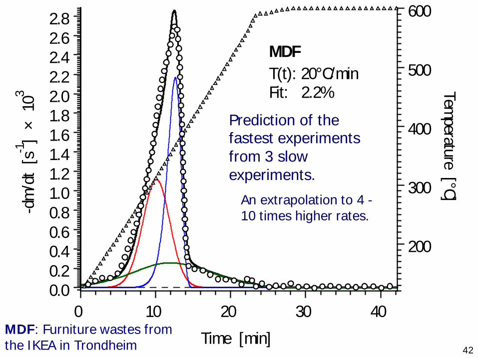
42Time [min]

-dm

/dt

[s-1]

× 1


0 10 20 30 40

MDFT(t): 20°C/minFit: 2.2%


0.00.20.40.60.81.01.21.41.61.82.02.22.42.62.8

200

300

400

500

600



MDF: Furniture wastes from the IKEA in Trondheim

43

End of the Introduction.Thanks for your attention. But we have not finished yet all . . .

introduction to kinetic models for biomass pyrolysis....

Documents