introduction to international finance - www ... · hochschule esslingen international finance slide...
TRANSCRIPT

Hochschule EsslingenInternational Finance slide 1
Introduction to International Finance
Prof. Dr. Frank Andreas Schittenhelm
Chapter 4

Hochschule EsslingenInternational Finance slide 2
Literature
Basic LiteratureRoss/Westerfield/Jordan: Fundamentals of Corporate Finance, 6thed., Irwin
McGraw-HillEun/Resnick: International Financial Management, Irwin McGraw-Hill
Additional LiteratureArnold: Corporate Financial Management, 2nded., Prentice HallGünther/Schittenhelm: Investition und Finanzierung, Schaeffer-Poeschel

Hochschule EsslingenInternational Finance slide 3
Table of Contents
Introduction to International Finance1. Introduction2. International Accounting3. International Equity and Debt Financing4. International Investment Strategies5. Risk Management and Exchange Rates

Hochschule EsslingenInternational Finance slide 4
4. Introduction to International Finance Learning Target International Finance
The learning target of this chapter is to understand
the specific aspects of international finance,
the possibilities of international sources of finance,
different investment strategies,
how a company can deal with exchange rate risk,
measures used in financial risk management.

Hochschule EsslingenInternational Finance slide 5
4. Introduction to International Finance 4.1. Introduction
General Tasks of Financial ManagementInvestmentsCapital structureDividend policyWorking capital managementShareholder value maximization
Particularities of International Financial ManagementForeign exchange rate riskPolitical riskImperfect marketsAdditional market opportunities

Hochschule EsslingenInternational Finance slide 6
4. Introduction to International Finance 4.1. Introduction (2)
Reasons for the Necessity of International Financial ManagementGlobalisation
Computer and telecommunicationReduction of transportation costs
LiberalisationGATT (General Agreement on Tariffs and Trade)WTO (World Trade Organisation)EU (European Union), NAFTA (North American Free Trade Agreement)
Deregulation and PrivatisationFinancial markets (new products, cross border listings, free commission etc.)Telecommunication, energy etc.
Multinational enterprisesTreasurer
Hochschule EsslingenInternational Finance slide 7
4. Introduction to International Finance 4.3. International Equity and Debt Financing
Characteristics of the Euro marketsMarket participants
BanksGovernmental institutionsCorporations with high rating
Business volume: several million Location
few regulations by the authoritiesLondon, Luxemburg, New York, TokyoOff-shore centres: Bahamas, Caiman, Singapore, Hong-Kong
Syndicate of banksLead manager (arranger): leading feeUnderwriting bank (underwriters): fee for guarantyPlacing agents (sellers)
Hochschule EsslingenInternational Finance slide 8
4. Introduction to International Finance 4.3.1. International Equity Financing
Stock Exchanges around the WorldUnited States
American Stock Exchange (AMEX) Arizona Stock Exchange Chicago Stock Exchange NASDAQ New York Stock ExchangePacific Exchange (Los Angeles and San Francisco) Philadelphia Stock Exchange
World Markets
Abidjan Stock Exchange African Stock Exchange Guide Alberta Stock Exchange Athens Stock Exchange Australian Stock ExchangeBangalore Stock Exchange Barcelona Stock Exchange Bavarian Stock Exchange (Munich) Beirut Stock Exchange Berlin Stock ExchangeBermuda Stock Exchange Bilbao Stock Exchange Bogotá Stock Exchange Botswana Stock Exchange Brussels Stock ExchangeBucharest Stock Exchange Budapest Stock Exchange Buenos Aires Stock Exchange Bulgarian Stock Exchange Cairo Stock ExchangeCaracas Stock Exchange Casablanca Stock Exchange Chile Electronic Stock Exchange Colombo Stock ExchangeCopenhagen Stock Exchange Costa Rica National Stock Exchange Cyprus Stock Exchange German Stock ExchangeGhana Stock Exchange Guayaquil Stock Exchange Helsinki Stock Exchange Hiroshima Stock Exchange Hong Kong Stock ExchangeIndian Stock Exchange (NSE) Istanbul Stock Exchange Italian Stock Exchange Jakarta Stock Exchange Jamaica Stock ExchangeJohannesburg Stock Exchange Karachi Stock Exchange Korea Stock Exchange Lahore Stock Exchange Lima Stock ExchangeLisbon Stock Exchange Ljubljana Stock Exchange London Stock Exchange Lusaka Stock Exchange Luxembourg Stock ExchangeMacedonian Stock Exchange Madrid Stock Exchange Mangalore Stock Exchange Mauritius Stock Exchange (SEM) Medellin Stock ExchangeMexican Stock Exchange Montreal Stock Exchange Moscow Central Stock Exchange Nagoya Stock Exchange Nairobi Stock ExchangeNamibian Stock Exchange New Zealand Stock Exchange Nicaragua Stock Exchange Nigerian Stock ExchangeNijny Novgorod Stock and Currency Exchange (in Russian) Occident Stock Exchange (Cali) Oslo Stock Exchange Panama Stock ExchangeParis Stock Exchange Prague Stock Exchange Rhenish-Westphalian Stock Exchange (Dusseldorf) Santiago Stock ExchangeSao Paulo Stock Exchange Shanghai Stock Exchange Shenzhen Stock Exchange Singapore Stock Exchange St. Petersburg Stock ExchangeStockholm Stock Exchange Swaziland Stock Market Taiwan Stock Exchange Tallinn Stock Exchange Tanzanian Stock ExchangeTehran Stock Exchange Tel Aviv Stock Exchange Thailand Stock Exchange Tokyo Stock Exchange Toronto Stock ExchangeTunis Stock Exchange Ural Stock Exchange Vancouver Stock Exchange Venezuelan Electronic Stock Exchange Vienna Stock Exchange Warsaw Stock Exchange Zagreb Stock Exchange Zimbabwe Stock Exchange Zurich Stock Exchange

Hochschule EsslingenInternational Finance slide 9
4. Introduction to International Finance 4.3.1. International Equity Financing (2)
Reasons for Cross-border ListingsBroaden shareholder basisDomestic stock exchange is too smallReward employees in foreign countriesBetter understanding of the firm’s strategyRaise awareness of the companyImprove disciplineUnderstand better the economic, social and industrial changes occurring in major markets
Hochschule EsslingenInternational Finance slide 10
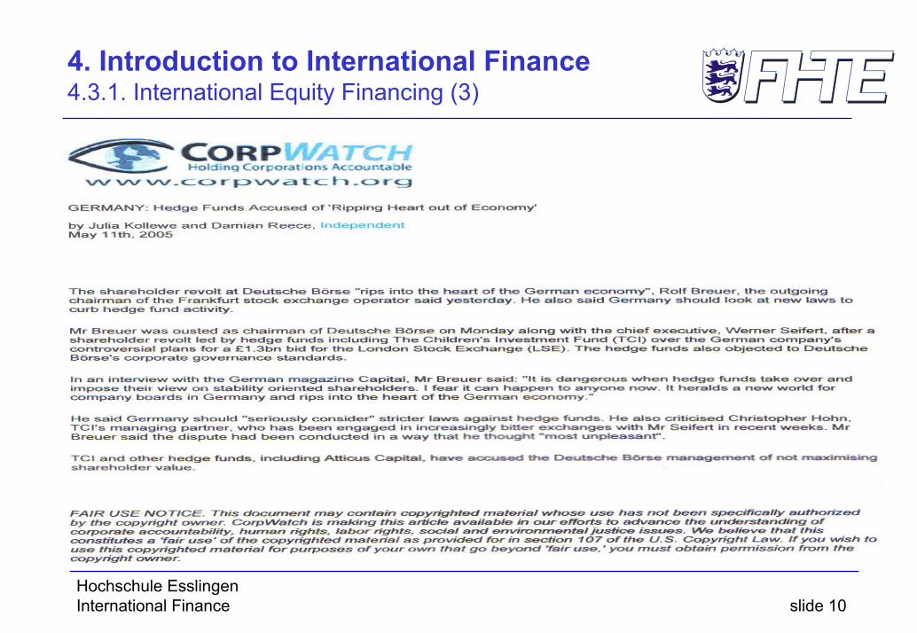
4. Introduction to International Finance 4.3.1. International Equity Financing (3)
Artikel Deutsche Börse

Hochschule EsslingenInternational Finance slide 11
4. Introduction to International Finance 4.3.2. International Bond Market
Overview
Bond marketsBond markets
International bond marketsInternational bond marketsDomestic marketsDomestic markets
Foreign bondsForeign bonds EurobondsEurobonds
Hochschule EsslingenInternational Finance slide 12
4. Introduction to International Finance 4.3.2. International Bond Market (2)
Foreign BondBond denominated in the currency of the country where it is issued.Issuer is a non-resident.
EurobondBonds sold outside the jurisdiction of the country of the currency in which the bond is denominated
AdvantagesEurobonds are not subject to rules and regulations like foreign bonds.Eurobonds are not subject to an interest-withholding tax.Eurobonds are bearer bonds (holders don’t have to disclose identity)

Hochschule EsslingenInternational Finance slide 13
4. Introduction to International Finance 4.3.2. International Bond Market (3)
Types of EurobondsStraight fixed-rate bond
Coupon constant over time, coupon payment annuallyEquity related bond
Bonds with warrants attached:Option to buy some other asset (e.g. shares) at a preset price in the future. Warrants are detachable.Convertibles:Bondholder has the right to convert the bond into ordinary shares at a preset price.
Floating-rate notes (FRN’s)Variable coupon reset on a regular basis (e.g. every 3 / 6 months) in relation to a reference rate (e.g. LIBOR)Variations: Capped Note, Floor Note, Collared Note
Hochschule EsslingenInternational Finance slide 14
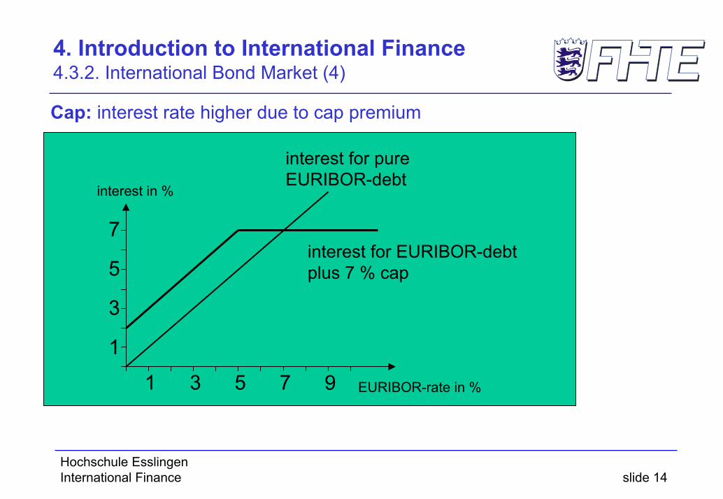
4. Introduction to International Finance 4.3.2. International Bond Market (4)
Cap: interest rate higher due to cap premium
EURIBOR-rate in %
interest in %
1
7
5
3
1 3 5 7 9
interest for pureEURIBOR-debt
interest for EURIBOR-debt plus 7 % cap
Hochschule EsslingenInternational Finance slide 15
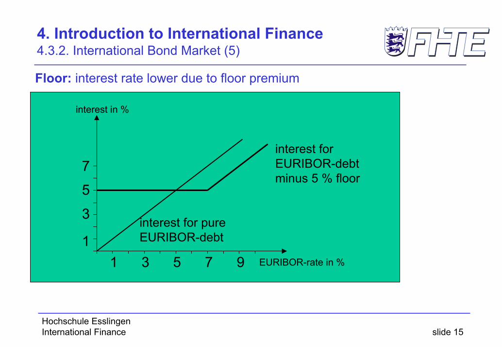
4. Introduction to International Finance 4.3.2. International Bond Market (5)
Floor: interest rate lower due to floor premium
EURIBOR-rate in %
1
7
5
3
1 3 5 7 9
interest for pureEURIBOR-debt
interest forEURIBOR-debt minus 5 % floor
interest in %

Hochschule EsslingenInternational Finance slide 16
4. Introduction to International Finance 4.3.2. International Bond Market (6)
Collar: pay cap premium get floor premium
EURIBOR-rate in %
interest in %
1
75
3
1 3 5 7 9
interest for pureEURIBOR-debt
interest forEURIBOR-debt plus Collar

Hochschule EsslingenInternational Finance slide 17
4. Introduction to International Finance 4.3.2. International Bond Market (7)
Advantages and Drawbacks of Eurobonds
1. Only for large companies2. Safe storage is needed (bearer
bonds!)3. Exchange-rate risk might occur4. Secondary market might be illiquid
1. Large amounts and long periods available
2. Often cheaper because of missing tax deduction, less regulations
3. Hedging: interest rates and exchange-rate risk
4. Bonds are unsecured, therefore less limitations for placement
5. Greater innovations and tailor-made financial solutions because of less regulations
DrawbacksAdvantages
Hochschule EsslingenInternational Finance slide 18
4. Introduction to International Finance 4.3.3. International Debt Financing
Euro Medium-term NotesIssuing of notes by syndicate of banks (arranger, underwriters, placing agents)Unsecured lendingMaturity 9 month and upNote issuance facility: Revolving Underwriting Facility, Note Standby Facility
Eurocommercial paperUnsecured lending, available only to corporations with highest credit rankingShort-term IOU, normal range 30-90 daysNormally issued at a discount, no coupon paymentsIssued and placed outside the jurisdiction of the country in whose currency it is denominatedAdvantage for lender: higher interest rate than for depositing in bankAdvantage for borrower: no fee must be paid to bank intermediaryCommercial paper programme: Roll-over issue possible with bank as underwriter

Hochschule EsslingenInternational Finance slide 19
4. Introduction to International Finance 4.4. International Investment Strategies
General Aspects of International Investments
AdvantagesDiversificationProduct innovationsMarkets with less restrictionsTax advantages
DisadvantagesUnknown marketsUnknown regulationsTax disadvantages

Hochschule EsslingenInternational Finance slide 20
4. Introduction to International Finance 4.4.1. Stock markets
Portfolio Theory and DiversificationExampleAn investor plans to invest 1.000 €. The chosen share earns 10 % in the good case (probability 40%) and 2 % otherwise.The function W describes the final wealth of the investors with Wgood und Wbad.
Es gilt also:C = 1.000 €, igood = 10%, ibad = 2% and p = 40%.Wgood = 1.000 € * (1+10%) = 1.100 € and Wbad = 1.000 € * (1+2%) = 1020 €.
The expected value of the function W is then:E(W) = 40%*1.100 € + 60% * 1020 € = 1.052 €

Hochschule EsslingenInternational Finance slide 21
4. Introduction to International Finance 4.4.1. Stock markets (2)
Example (continued)Additionally, consider a risk-free asset F with a fixed interest i = 5%. Suppose the investor invests x = 80% in the risky share.
The final wealth of the investors will be then:Wgood (80%) = 80% * 1.000 € * (1+10%) + 20% * 1.000 € * (1+5%) = 1.090 €Wbad (80%) = 80% * 1.000 € * (1+2%) + 20% * 1.000 € * (1+5%) = 1.026 €The expected value will be:E(W(80%)) = 40% * 1090 € + 60% * 1026 € = 1051,6 €.
The following table shows the values for different shares x: x 0% 20% 40% 60% 80% 100%
Wgood (x) 1050 1060 1070 1080 1090 1100
Wbad (x) 1050 1044 1038 1032 1026 1020
E(W(x)) 1050,0 1050,4 1050,8 1051,2 1051,6 1052,0

Hochschule EsslingenInternational Finance slide 22
4. Introduction to International Finance 4.4.1. Stock markets (3)
Risk-Return-Analysis (two risky assets)Basis of the analysis are three parameters:µA := Expected value of the return of asset A ,SD(A) = σA:= Standard deviation of the return of asset A ,ρA,B := Correlation coefficient of the return of A and B.
Consider a portfolio P with two risky assets A and B and shares of xA and xB of the total portfolio respectively, with .
By definition the expected values and standard deviations are given as follows:
and ,
1, =+⋅+⋅= BABA xxBxAxP
BA BEAE µµ == )(,)( BA BSDASD σσ == )(,)(

Hochschule EsslingenInternational Finance slide 23
4. Introduction to International Finance 4.4.1. Stock markets (4)
Risk-Return-Analysis (two risky assets)Determination of the parameters
Return of asset i between t-1 and t:
Empirical expected value of the return:
Empirical standard deviation:
Empirical covariance of two returns:
Empirical correlation coefficient:
( ) ( )( )1
1, −
−−=
tWtWtWR ti
( ) ∑=
⋅N
titii R
NAE
1, =: 1 = µ
( ) ( ) i
N
titii R
NAVar σµ :
11 = = )SD(A
1
2
,i =−⋅− ∑
=
( ) ( ) ji,
N
1tjtj,iti,ji :µRµR
1N1 = )A,COV(A δ=−⋅−⋅− ∑
=
ji
ji
σσδ
ρ⋅
= ,ji,

Hochschule EsslingenInternational Finance slide 24
4. Introduction to International Finance 4.4.1. Stock markets (5)
Risk-Return-Analysis (two risky assets)We consider the following (see chapter 0):
and
, since
The Diversification Effect
BBAABABA xxBExAExBxAxEPE µµ ⋅+⋅=⋅+⋅=⋅+⋅= )()()()(
)()(2)()()()( ,2222 BSDASDxxBSDxASDxBxAxSDPSD BABABABA ⋅⋅⋅⋅⋅+⋅+⋅=⋅+⋅= ρ
)()()()( BSDxASDxBxAxSDPSD BABA ⋅⋅ +⋅≤+⋅=
)()(2)()()( ,2222 BSDASDxxBSDxASDxPSD BABA ⋅⋅⋅⋅⋅+⋅+⋅= ΒΑρ
)()()()(2)()( 2222 BSDxASDxBSDASDxxBSDxASDx BABABA ⋅+⋅=⋅⋅⋅⋅+⋅+⋅≤

Hochschule EsslingenInternational Finance slide 25
4. Introduction to International Finance 4.4.1. Stock markets (6)
Risk-Return-Analysis (two risky assets)
return µ
risk σA
efficient portfolios B
correlation ρ =+1X*
ρ =-1
-1<ρ<+1 X

Hochschule EsslingenInternational Finance slide 26
4. Introduction to International Finance 4.4.1. Stock markets (7)
Risk-Return-Analysis (for risky assets and risk-free asset)Suppose there exists a risk-free asset F
Formally: The return of F is fixed with: .For a combination C (of a risky portfolio P and F) results:
The risk of the combination C can be described as follows:
with .
Solving for x: .
The return of combination C is then:
There is a linear relation between expected value and standard deviation of C.
FxPxC ⋅−+⋅= )1(
Fµ 0=Fσ
PFFPPFC xxxx ,2222 )1(2)1( ρσσσσσ −++−=
PPCFF xx σσσσσ ==== 222 therefore and 0,0
P
Cxσσ
=
CP
FPFF
P
CP
P
Cc σ
σµµµµ
σσµ
σσµ )()1( −
+=−+=
Hochschule EsslingenInternational Finance slide 27
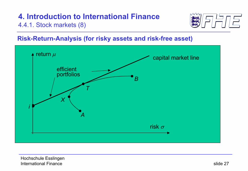
4. Introduction to International Finance 4.4.1. Stock markets (8)
Risk-Return-Analysis (for risky assets and risk-free asset)
return µ
risk σ
A
B
capital market line
T
efficientportfolios
Xi
Hochschule EsslingenInternational Finance slide 28
4. Introduction to International Finance 4.4.1. Stock markets (9)
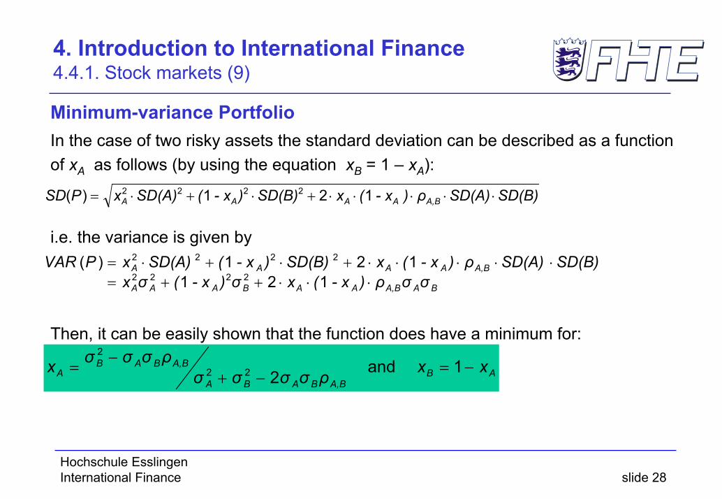
Minimum-variance PortfolioIn the case of two risky assets the standard deviation can be described as a function of xA as follows (by using the equation xB = 1 – xA):
i.e. the variance is given by
Then, it can be easily shown that the function does have a minimum for:
ABΑ,ΒBABA
Α,ΒBABA xxρσσσσ
ρσσσx −=−+
−= 1and222
2
SD(B)SD(A)ρ ) - x(xSD(B)) - x(SD(A)xPSD Α,ΒAAAA ⋅⋅⋅⋅⋅+⋅+⋅= 121)( 2222
BAΑ,ΒAABAAA
Α,ΒAAAA
σσρ) - x(xσ) - x(σxSD(B)SD(A)ρ) - x(xSD(B)) - x(SD(A)xPVAR
⋅⋅⋅++=⋅⋅⋅⋅⋅+⋅+⋅=
121121)(
2222
2222

Hochschule EsslingenInternational Finance slide 29
4. Introduction to International Finance 4.4.1. Stock markets (10)
Minimum-variance PortfolioExampleShare A with µ=8% ; σ=12% and share B with µ=13 % ; σ = 20%.
Case 1: ρA,B = 0,3
and xB = 18 %with E(P) = 0,82 ⋅ 8 % + 0,18 ⋅ 13 % = 8,9 % and SD(P) = 11,4%.
Case 2: ρA,B= –1xA = 20/32 = 62,5 % and xB = 12/32 = 37,5 %with E(P) = 0,625 ⋅ 8 % + 0,375 ⋅ 13 % = 9,875 % and SD(P) = 0.
%820072,0204,00144,00072,004,0 =⋅−+
−=Ax

Hochschule EsslingenInternational Finance slide 30
4. Introduction to International Finance 4.4.2. Bond markets
Example: Price (market) riskAn investor purchases a bond 1 for 100 € at time t=0. The coupon payment is 7 €. The market return is r=7% at t=0.
The present value (or price) of the bond is therefore:
After one year the investor decides to sell the bond. The price at t=1 depends once again from the current required market return.
a) For r=5%:
b) For r=7%:
c) For r=9%:
72,103%)51(
107%)51(
7%)5( 21 =+
++
=V
100%)71(
107%)71(
7%)7( 21 =+
++
=V
48,96%)91(
107%)91(
7%)9( 21 =+
++
=V
100%)71(
107%)71(
7%)71(
7%)7( 321 =+
++
++
=V

Hochschule EsslingenInternational Finance slide 31
4. Introduction to International Finance 4.4.2. Bond markets (2)
Example: Reinvestment riskThe investor acquires the bond from the previous example, expecting 7% interest gains over 3 years. At time T=3 the total capital is expected to be:
In fact, the investor receives coupon payments at time t = 1 and t= 2. These payments of 7 € respectively must be reinvested at current market conditions.
Changes of the market required return cause the following consequences: Total wealth at time T = 3:a) For r=5%:
b) For r=7%:
c) For r=9%:
50,12207,1100 3 =⋅
07,122107%)51(7%)51(7%)5( 2 =++⋅++⋅=W
50,122107%)71(7%)71(7%)7( 2 =++⋅++⋅=W
95,122107%)91(7%)91(7%)9( 2 =++⋅++⋅=W

Hochschule EsslingenInternational Finance slide 32
4. Introduction to International Finance 4.4.2. Bond markets (3)
Modified DurationDefinitionThe Modified Duration is defined by:
.
This form of duration has been developed by Hicks 1939. Other expressions are Adjusted Duration or Volatility.
Modified Duration is used as a sensitivity measure and to estimate price changes.
∑
∑
=
−
=
−−
+⋅
+⋅⋅=⋅−= T
t
tt
T
t
tt
rc
rct
VdrdVMD
1
1
1
)1(
)1(1
Hochschule EsslingenInternational Finance slide 33
4. Introduction to International Finance 4.4.2. Bond markets (4)
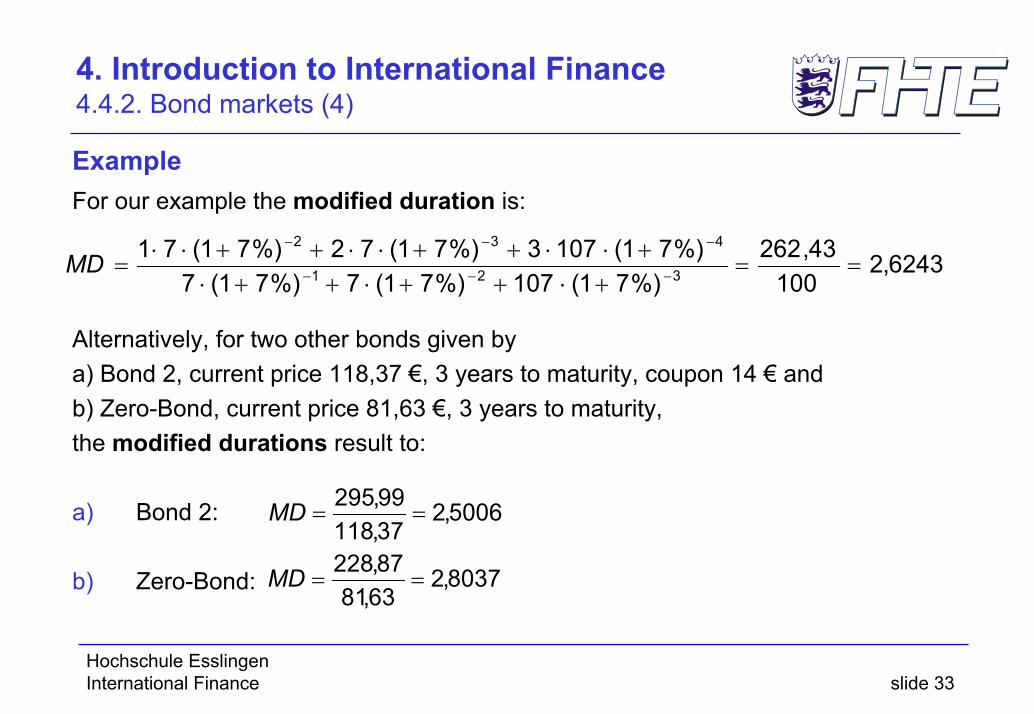
ExampleFor our example the modified duration is:
Alternatively, for two other bonds given bya) Bond 2, current price 118,37 €, 3 years to maturity, coupon 14 € andb) Zero-Bond, current price 81,63 €, 3 years to maturity,the modified durations result to:
a) Bond 2:
b) Zero-Bond:
6243,2100
43,262%)71(107%)71(7%)71(7
%)71(1073%)71(72%)71(71321
432
==+⋅++⋅++⋅
+⋅⋅++⋅⋅++⋅⋅= −−−
−−−
MD
5006,237,11899,295
==MD
8037,263,8187,228
==MD

Hochschule EsslingenInternational Finance slide 34
4. Introduction to International Finance 4.4.2. Bond markets (5)
Macaulay DurationBy multiplying the modified duration with (1 + r ) one receives the Macaulay Duration D.
DefinitionThe Macaulay Duration is defined by:
This form of duration was developed by Frederick Macaulay in 1938.
∑
∑
=
−
=
−
+⋅
+⋅⋅=+⋅= T
t
tt
T
t
tt
rc
rctrMDD
1
1
)1(
)1()1(

Hochschule EsslingenInternational Finance slide 35
4. Introduction to International Finance 4.4.2. Bond markets (6)
Bond Price EstimationExampleGiven our previous example of bond 1,we receive the following bond prices if the market interest rate changes:
If we estimate the price changes with modified duration we apply:
and therefore, we receive:
45,105%)51(
107%)51(
7%)51(
7%)5( 321 =+
++
++
=V
94,94%)91(
107%)91(
7%)91(
7%)9( 321 =+
++
++
=V
)()()( rVrMDrVrrV ⋅∆⋅−≈∆+
25,105100%)2(6243,2100)()(%))2(%7( =⋅−⋅−=⋅∆⋅−≈−+ rVrMDrVV75,94100%26243,2100)()(%)27( =⋅⋅−=⋅∆⋅−≈+ rVrMDrVV
Hochschule EsslingenInternational Finance slide 36
4. Introduction to International Finance 4.4.2. Bond markets (7)
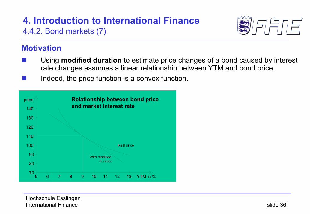
MotivationUsing modified duration to estimate price changes of a bond caused by interest rate changes assumes a linear relationship between YTM and bond price. Indeed, the price function is a convex function.
70
80
90
100
110
120
130
140
5 6 7 8 9 10 11 12 13 YTM in %
price
Real price
With modified duration
Relationship between bond price and market interest rate

Hochschule EsslingenInternational Finance slide 37
4. Introduction to International Finance 4.4.2. Bond markets (8)
ConvexityDefinitionThe convexity is defined by:
.
And we can apply the following approximation:
∑
∑
=
−
=
−−
+⋅
+⋅⋅+⋅=⋅= T
t
tt
T
t
tt
rc
rctt
VdrVdC
1
1
2
2
2
)1(
)1()1(1
)()(21)()()( 2 rVrCrVrMDrVrrV ⋅∆⋅⋅+⋅∆⋅−≈∆+

Hochschule EsslingenInternational Finance slide 38
4. Introduction to International Finance 4.4.2. Bond markets (9)
ExampleWe consider the following investment alternatives:
Zero-bond 1: current price 81.6298; 3 years time to maturity Bond portfolio with cash flow (-81.6298; 0; 46.7290; 0; 53.5000),
Actually, the bond portfolio consists of two zero-bonds (with 40.8149 investment in each of the two bonds):Zero-bond 2: current price 87.3439; 2 years time to maturity andZero-bond 3: current price 76,2895; 4 years time to maturity
Investment (prices) of both alternatives are the same. The modified duration is for both alternatives is 2.8037. The convexity for zero-bond 1 is: C = 10,4813The convexity for the portfolio is: C = 11,3547

Hochschule EsslingenInternational Finance slide 39
4. Introduction to International Finance 4.4.2. Bond markets (10)
Example (continued)An instant interest rate change will lead to the following new prices of the alternatives:
In both cases an investment in the portfolio is advantageous due to the higher convexity.
r zero-bond 1 portfolio
5% V(5%) = 86,3838 V(5%) = 86,3992
7% V(7%) = 81,6298 V(7%) = 81,6298
9% V(9%) = 77,2183 V(9%) = 77,2316

Hochschule EsslingenInternational Finance slide 40
4. Introduction to International Finance 4.4.2. Bond markets (11)
price function with different convexities
7%
-50
0
50
100
150
200
250
300
0% 2% 4% 6% 8% 10% 12% 14% 16% 18% 20%
market interest rate
pric
e / v
alue low convexity
approximation with md
high convexity

Hochschule EsslingenInternational Finance slide 41
4. Introduction to International Finance 4.4.2. Bond markets (12)
Exercise
a) The current price of a zero-bond is 680,58 €; face value 1000 €; time to maturity 5 years. What is the current market interest rate? Determine the Macaulay duration.
b) The current price of a bond is 100 €; face value 100 €; current market interest rate is 9%; time to maturity 3 years. What is the annual coupon payment?Estimate the new bond prices using duration and convexity for the following yield shift: (+2.0).
Hochschule EsslingenInternational Finance slide 42
4. Introduction to International Finance 4.4.2. Bond markets (13)
Solution

Hochschule EsslingenInternational Finance slide 43
4. Introduction to International Finance 4.4.2. Bond markets (14)
Bond Investment StrategiesBuy and Hold StrategyBonds are kept until time to maturity.Cash Flow MatchingCoupon and principal payments are matched to liability structure. Duration MatchingMacaulay duration of a portfolio equals the investment horizon.ImmunisationStructure assets and liabilities according to duration gap.Riding the Yield CurveTime to maturity of bonds longer than liability structure.

Hochschule EsslingenInternational Finance slide 44
4. Introduction to International Finance 4.4.2.1. Cash Flow Matching
Description of the strategy1. Identification of liability structure:
Determination of amount and maturity of liabilitiesDetermination of fixed planning horizon
2. Determination of relevant investment restrictions:E.g. rating, minimum and maximum investment amounts.
3. Applying a cash flow matching strategy:Step 1: choose bond with time to maturity equal to maturity of longest liability,coupon and principal payment at time to maturity must cover total liability, earlier coupon payments reduce earlier liabilities.Step 2: choose bond with time to maturity equal prior liability (consider coupon payments of bond 1). Repeat for all maturities.

Hochschule EsslingenInternational Finance slide 45
4. Introduction to International Finance 4.4.2.1. Cash Flow Matching (2)
ExampleAn investor determines the following liability structure which he wants to cover with a cash flow matching strategy:
at time t=1, t=2, t=3, t=4: 100.000 €
The following bond are available:Bond 1 with (-100; 7; 7; 107),Bond 3 with (-102; 8; 8; 8; 108),Bond 4 with (-94; 5; 105),Bond 5 with (-95; 103).
In addition we consider:Zero-Bond with (-81,63; 0; 0; 100)

Hochschule EsslingenInternational Finance slide 46
4. Introduction to International Finance 4.4.2.1. Cash Flow Matching (3)
Time t=4 t=3 t=2 t=1 t=0Remaining liabilities 100.000 100.000 100.000 100.000
Bond 3 926
Revenues 100.008 7.408 7.408 7.408 -94.452Remaining liabilities 92.592 92.592 92.592
Bond 1 866
Revenues 92.662 6.062 6.062 -86.600Remaining liabilities 86.530 86.530
Bond 4 825
Revenues 86.625 4.125 -77.550Remaining liabilities 82.405
Bond 5 801
Revenues 82.503 -76.095Total investment -334.697

Hochschule EsslingenInternational Finance slide 47
4. Introduction to International Finance 4.4.2.1. Cash Flow Matching (4)
Time t=4 t=3 t=2 t=1 t=0Remaining liabilities 100.000 100.000 100.000 100.000
Bond 3 926
Revenues 100.008 7.408 7.408 7.408 -94.452Remaining liabilities 92.592 92.592 92.592
Zero-Bond 926
Revenues 92.600 0 0 -75.589Remaining liabilities 92.592 92.592
Bond 4 882
Revenues 92.610 4.410 -82.908Remaining liabilities 88.182
Bond 5 857
Revenues 88.271 -81.415Total investment -334.364

Hochschule EsslingenInternational Finance slide 48
4. Introduction to International Finance 4.4.2.1. Cash Flow Matching (5)
ExerciseThe following liabilities are given:at time t = 1: 1.000.000 €; at t = 2: 2.000.000 €; at t = 3: 3.000.000 €The following bonds are available:1. Bond 1: price: 100; coupon 8; time to maturity 3 years2. Bond 2: price: 102; coupon 9; time to maturity 2 years3. Bond 3: price: 104; coupon 10; time to maturity 1 year4. Bond 4: price: 89; coupon 3; time to maturity 1 yearApply a cash flow matching strategy and minimize the investors investment.

Hochschule EsslingenInternational Finance slide 49
4. Introduction to International Finance 4.4.2.1. Cash Flow Matching (6)
Solution

Hochschule EsslingenInternational Finance slide 50
4. Introduction to International Finance 4.4.2.2. Duration Matching
DefinitionA portfolio is matched, if the Macaulay duration of the portfolio equals the investment horizon.
ExampleGiven bond 1, the Macaulay Duration is D=2,8080.The total value of an investment for different yield scenarios at t = 2,8080 is then:
Any interest rate change implies an increase of the portfolio value at t = 2,8080 .
Yield r 5% 6,5% 7% 7,5% 9%
Bond price 106,0024 105,7142 105,6191 105,5247 105,2443
Reinvestment of coupons
14,9270 15,2096 15,3042 15,3991 15,6850
Total value 120,9294 120.9238 120,9233 120,9238 120,9293

Hochschule EsslingenInternational Finance slide 51
4. Introduction to International Finance 4.4.2.2. Duration Matching (2)
Example
0 2 31D
Price
-DiPV+Di
+Di
FV-Di
time

Hochschule EsslingenInternational Finance slide 52
4. Introduction to International Finance 4.4.2.2. Duration Matching (3)
Mathematical backgroundTo determine: minimum of the function
We know:
∑=
−∆++⋅⋅∆++=∆T
t
tt rrcrrrf
1)1()1()( τ
∑∑=
−−
=
−− ∆++⋅⋅−⋅∆+++∆++⋅⋅∆++⋅=∆′T
t
tt
T
t
tt rrctrrrrcrrrf
11
1 )1()1()1()1()( τττ
∑=
−+−∆++⋅⋅−+−⋅+−=∆′′T
t
tt rrcttrf
1
2)1()1()()( τττ
1

Hochschule EsslingenInternational Finance slide 53
4. Introduction to International Finance 4.4.2.2. Duration Matching (4)
Mathematical backgroundThe necessary condition for a minimum is therefore .Solve equation for τ:
Check for local minimum.
01
1
01
1 )1()1()1()1(=∆=
−−
=∆=
−− ∑∑ ∆++⋅⋅⋅∆++=∆++⋅⋅∆++⋅r
T
t
tt
r
T
t
tt rrctrrrrcrr τττ
01
1
1
0
1
)1(
)1(
)1()1(
=∆=
−
=
−−
=∆
−
∑
∑
∆++⋅
∆++⋅⋅=
∆++∆++⋅
⇒
r
T
t
tt
T
t
tt
r rrc
rrct
rrrrτ
ττ
Drc
rct
rc
rctr T
t
tt
T
t
tt
T
t
tt
T
t
tt
=+⋅
+⋅⋅=
+⋅
+⋅⋅⋅+=⇒
∑
∑
∑
∑
=
−
=
−
=
−
=
−−
1
1
1
1
1
)1(
)1(
)1(
)1()1(τ
0)( >∆′′ rf

Hochschule EsslingenInternational Finance slide 54
4. Introduction to International Finance 4.4.2.3. Duration-gap Analysis
AssumptionsAssume unique interest rate for assets and liabilities.
Net value of company can be calculated by:
Changes of the interest rate can be described by (r given):
Define duration gap:
where MD A und MD L are the modified durations of total assets and liabilities respectively.The net value is immunized against interest rate changes if the duration gap equals 0:
∑∑=
−
=
− +⋅−+⋅=T
t
tLt
T
t
tAt rcrcrN
11)1()1()(
∑∑=
−
=
− ∆++⋅−∆++⋅=∆T
t
tLt
T
t
tAt rrcrrcrN
11)1()1()(
LA MDMD −
0=− LA MDMD

Hochschule EsslingenInternational Finance slide 55
4. Introduction to International Finance 4.4.2.3. Duration-gap Analysis (2)
Mathematical background1) necessary condition:
00
=∆ =∆rrN
∂∂
01
01 )1()1(
=∆+
=∆+ ∑∑ +
⋅−=
+⋅−
⇔r
t
Lt
rt
At
rct
rct
0
1
0
1
)1()1(
)1()1(
=∆
−
−−
=∆
−
−−
∑∑
∑∑
+⋅+⋅⋅−
=+⋅+⋅⋅−
⇔r
tLt
tLt
rtA
t
tAt
rcrct
rcrct
LA MDMD =⇔

Hochschule EsslingenInternational Finance slide 56
4. Introduction to International Finance 4.4.2.3. Duration-gap Analysis (3)
Mathematical background2) sufficient condition:
00
2
2
≥∆
=∆rrN
∂∂
02
02 )1(
)1()1(
)1(
=∆+
=∆+ ∑∑ +
⋅−−⋅−≥
+⋅−−⋅−
⇔r
t
Lt
rt
At
rctt
rctt
0
2
0
2
)1()1()1(
)1()1()1(
=∆
−
−−
=∆
−
−−
∑∑
∑∑
+⋅+⋅⋅+⋅
≥+⋅
+⋅⋅+⋅⇔
rtL
t
tLt
rtA
t
tAt
rcrctt
rcrctt
LA CC ≥⇔

Hochschule EsslingenInternational Finance slide 57
4. Introduction to International Finance 4.4.2.3. Duration-gap Analysis (4)
ExerciseThe liabilities of Speedy GmbH can be described by the following cash flow:(+100.000; -7.000; -7.000; -107.000). The current interest rate for assets and liabilities is 7%.The responsible portfolio manager of the Speedy GmbH examines the following investment (asset) strategies:Cash flow from investment strategy 1: (-100.000; 0; 21.980; 98985,7)Cash flow from investment strategy 2: (-100.000; 0; 68.235; 0; 52.957,3496)Cash flow from investment strategy 3: (-100.000; 0; 68.000; 0; 53.226,401)Cash flow from investment strategy 4: (-100.000; 0; 68.500; 0; 52.653,951)Calculate for all strategies modified duration and explain by applying duration-gap analysis which of the strategies are suitable. (Hint: convexity of strategy 1: C = 9,4752; convexity of strategy 2: C = 10,1809)
Hochschule EsslingenInternational Finance slide 58
4. Introduction to International Finance 4.4.2.3. Duration-gap Analysis (5)
Solution
Hochschule EsslingenInternational Finance slide 59
4. Introduction to International Finance 4.4.2.4. Riding the Yield Curve
AssumptionsNecessary condition
Normal (upward sloping) yield curveStrategy
investor buys bonds with time to maturity longer than maturity of liabilities.
Decreased or unchanged yield structure:Selling before time to maturity generates higher returns than pure cash flow matchingReasons:
Higher YTM during investment horizon.Additional gains due to increase of bond prices.
Increase of yield curve:Bond prices fall risk of loss

Hochschule EsslingenInternational Finance slide 60
4. Introduction to International Finance 4.4.2.4. Riding the Yield Curve (2)
ExampleZero-bond 1 (-90,53; 0; 100); Zero-bond 2 (-86,01; 0; 0; 100)Investor‘s liabilities at t=2: 100.000 €
Yield curve: 5% for 1 year; 5,1% for 2 years; 5,15% for 3 years
4,7
4,8
4,9
5
5,1
5,2
5,3
t=1 t=2 t=3
Shift -0,1
Zinsstrukturkurve
Shift +0,1
Current yield curve

Hochschule EsslingenInternational Finance slide 61
4. Introduction to International Finance 4.4.2.4. Riding the Yield Curve (3)
ExampleZero-bond 1 (-90,53; 0; 100); Zero-bond 2 (-86,01; 0; 0; 100)investment 90.530 €:? 1000 of Zero-bond 1 or 1052,55 of Zero-bond 2
Prices for zero-bond 2 at t=2:shift = 0
bond price: 95,24; portfolio value: 100.245 €shift = +0,1
bond price: 95,15; portfolio value: 100.150 €shift = -0,1
bond price: 95,33; portfolio value: 100.340 €shift = +0,3
bond price: 94,97; portfolio value: 99.961 €
Hochschule EsslingenInternational Finance slide 62
4. Introduction to International Finance 4.4.2.4. Riding the Yield Curve (4)
ExerciseThe following liabilities are given:t = 1: 1.000.000 €; t = 2: 1.000.000 €An investor can choose from the following bonds:
bond 1: (-100; 7; 107)bond 2: (-100; 106)
Compare the strategies ‘cash-flow-matching’ and ‘riding-the-yield-curve’. Which one is better if you assume that the yield curve is not going to change? Calculate the necessary investments for both strategies.

Hochschule EsslingenInternational Finance slide 63
4. Introduction to International Finance 4.4.2.4. Riding the Yield Curve (5)
Solution: Cash-flow-matching
Hochschule EsslingenInternational Finance slide 64
4. Introduction to International Finance 4.4.2.4. Riding the Yield Curve (6)
Solution: Riding-the-yield-curve

Hochschule EsslingenInternational Finance slide 65
4. Introduction to International Finance 4.5. Risk Management and Exchange Rates
HedgingReducing a company’s exposure to price or rate fluctuations
Financial engineering
VolatilityPrice volatility (inflation)Interest rate volatilityExchange rate volatilityCommodity price volatility (basic goods and material)
The Risk Profile Risk profileof seller
Price change
Wea
lth c
hang
e
Risk profileof buyer
Price change
Wea
lthch
ange

Hochschule EsslingenInternational Finance slide 66
4. Introduction to International Finance 4.5.1. Options
TerminologyAn option contract is an agreement that gives the owner the right, but not the obligation, to buy or to sell an underlying asset at a fixed price, called the strike or exercise price, for a specified time.
CallsA call option is an option contract that gives the owner the right to buy an asset.PutsA put option is an option contract that gives the owner the right to sell an asset.
American OptionOption can be exercised within a specified period.European OptionOption can be exercised only on the expiration date.

Hochschule EsslingenInternational Finance slide 67
4. Introduction to International Finance 4.5.1. Options (2)
Features of an OptionType of Transaction (Put or Call)Style of Option (American or European)Name of IssuerUnderlying AssetExercise Price (Strike Price)Expiration Date
NotationC = Call priceP = Put priceS = Current price of the underlying assetST = Price of the asset on expiration dateX = Exercise price of the option

Hochschule EsslingenInternational Finance slide 68
4. Introduction to International Finance 4.5.1. Options (3)
AdvantagesHedging,High returns due to leverage,Possibility of portfolio insurance,Low capital investment necessary for an option deal.
DisadvantagesLimited time to maturity,New sources of risk, Complexity of products high standards requested from personnel, organisation, data processing, permanent supervision,Restricted range of product.
Hochschule EsslingenInternational Finance slide 69
4. Introduction to International Finance 4.5.1. Options (4)
Value of an OptionDefinitionAn option (call or put) is said to be at the money if the exercise price X practically corresponds to the current price S of the underlying asset.
DefinitionA call is said to be in the money if X is less than the current price S, correspondingly a put is in the money if X is greater than S.
DefinitionA call is said to be out of the money if X is greater than the current price S, correspondingly a put is said to be out of the money if X is less than S.

Hochschule EsslingenInternational Finance slide 70
4. Introduction to International Finance 4.5.1. Options (5)
Value of an Option at Expiration Date
(Intrinsic) Value of a Call on Expiration DateST - X for ST > X0 for ST < Xi.e. value of call = max (0, ST – X)
(Intrinsic) Value of a Put on Expiration Date0 for ST > XX - ST for ST < Xi.e. Value of put = max (0, X – ST)
Hochschule EsslingenInternational Finance slide 71
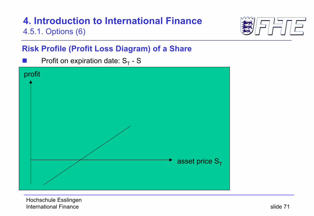
4. Introduction to International Finance 4.5.1. Options (6)
Risk Profile (Profit Loss Diagram) of a ShareProfit on expiration date: ST - S
asset price ST
profit

Hochschule EsslingenInternational Finance slide 72
4. Introduction to International Finance 4.5.1. Options (7)
Risk Profile Buying a CallProfit on expiration date: max (0, ST – X) – CBreak even for ST = X + CProfit if ST > X + C:
Maximum profit: unlimited maximum loss: - C
asset price ST
profit
-C

Hochschule EsslingenInternational Finance slide 73
4. Introduction to International Finance 4.5.1. Options (8)
ExampleYou purchase a call for C = 3 € with an exercise price of 40 €. Then, on expiration date you profit loss situation is as follows:
Remember: profit on expiration date is: max (0, ST – X) – C
max (0, ST – 40 €) – 3 € = – 3 €
max (0, ST – 40 €) – 3 € = ST – 43 €
ST ≤ 40 €
ST > 40 €
Profit / LossPrice Range
Hochschule EsslingenInternational Finance slide 74
4. Introduction to International Finance 4.5.1. Options (9)
ExerciseYou sell a call for C = 3 € with an exercise price of 40 €. Determine your profit loss situation on expiration date:
Solution

Hochschule EsslingenInternational Finance slide 75
4. Introduction to International Finance 4.5.1. Options (10)
Exercise Protective PutYou purchase a share at a current price of S = 54 € and a put on that underlying for P = 2 € with an exercise price of 50 €. Determine your profit loss situation on expiration date:Solution

Hochschule EsslingenInternational Finance slide 76
4. Introduction to International Finance 4.5.1. Options (11)
Exercise Covered CallYou purchase a share at a current price of S = 38 € and sell a call on that underlying for C = 3 € with an exercise price of 40 €. Determine your profit loss situation on expiration date:Solution

Hochschule EsslingenInternational Finance slide 77
4. Introduction to International Finance 4.6.1. Options (12)
Other Common Strategies
SpreadsCombination of several calls or several puts respectively
„Money Spreads”:Different exercise pricesEqual time to maturity
Bullish SpreadBearish Spread
StraddlesCombination of call(s) and put(s)
Long StraddleStraps = Bullish long StraddleStrips = Bearish long Straddle

Hochschule EsslingenInternational Finance slide 78
4. Introduction to International Finance 4.6.2. Forward Contracts, Futures and Swaps
DefinitionForward contracts are a legally binding agreement between two parties calling for the sale of an asset or product in the future at a price agreed upon today.
DefinitionFutures are standardized forward contracts with the feature that gains and losses are realized each day rather than only on the settlement day.
DefinitionSwap contracts are an agreement by two parties to exchange specified cash flows at specified intervals in the future.

Hochschule EsslingenInternational Finance slide 79
4. Introduction to International Finance 4.6.3. Hedging of Exchange Rate Risk
Example
The Computereinkauf GmbH must pay 200.000 US-Dollar for computers to its suppliers in 3 months.
Suppose:
Exchange rate today: 1,00 US$ = 1,00 €
Exchange rate in 3 months (1): 1,05 € ⇒ 210.000 €
Exchange rate in 3 months (2): 0,90 € ⇒ 180.000 €
Exchange rate in 3 months (3): 1,00 € ⇒ 200.000 €
Analyse the hedging possibilities of the company!

Hochschule EsslingenInternational Finance slide 80
4. Introduction to International Finance 4.6.3. Hedging of Exchange Rate Risk (2)
Immediate coverage:
Buy Dollars at current exchange rate
Invest Dollars
Interest Rate on investment depends on national situation (yield curve)
Advantages
Exchange rate is known
No additional costs
Disadvantages
Capital binding
Company can’t profit from exchange rate chances
Hochschule EsslingenInternational Finance slide 81
4. Introduction to International Finance 4.6.4. Hedging of Exchange Rate Risk (3)
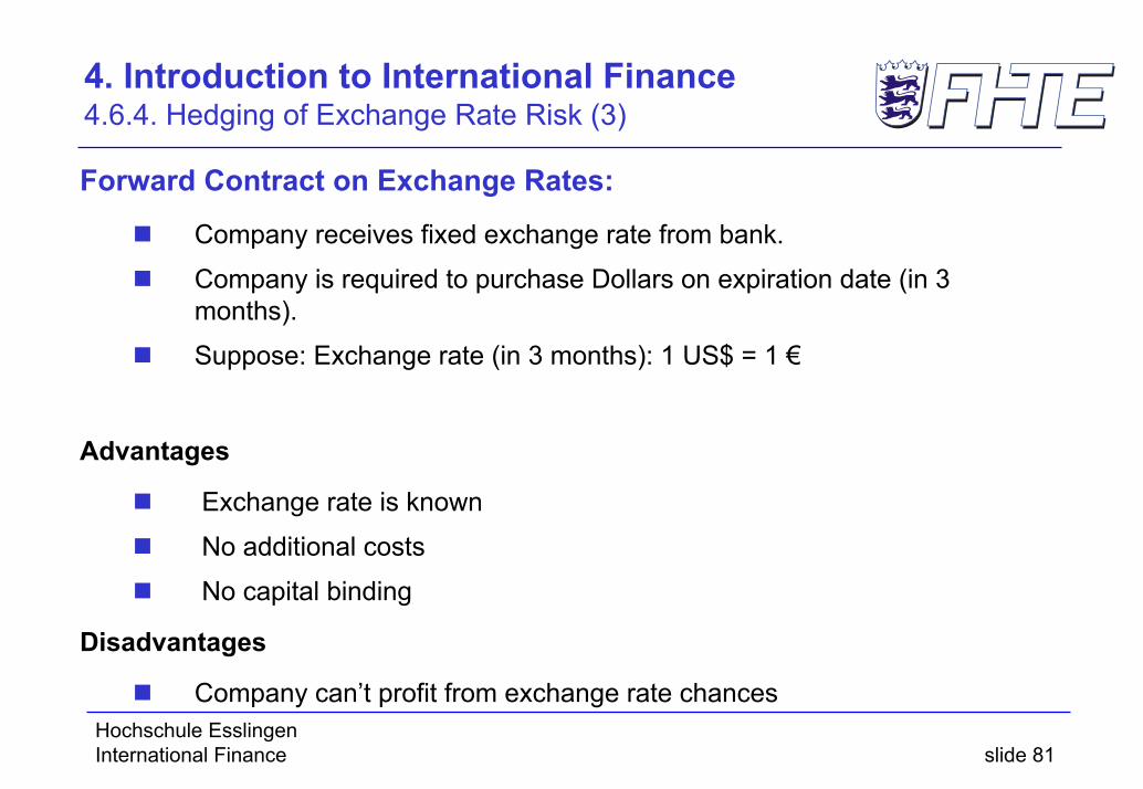
Forward Contract on Exchange Rates:
Company receives fixed exchange rate from bank.
Company is required to purchase Dollars on expiration date (in 3months).
Suppose: Exchange rate (in 3 months): 1 US$ = 1 €
Advantages
Exchange rate is known
No additional costs
No capital binding
Disadvantages
Company can’t profit from exchange rate chances

Hochschule EsslingenInternational Finance slide 82
4. Introduction to International Finance 4.6.4. Hedging of Exchange Rate Risk (4)
Option Contract on Exchange Rate:Computereinkauf GmbH purchases a call on Dollars.Right to purchase Dollars at a fixed price at a specified time (in 3 months).
Exercise price: 1US$ = 1 €Call price: 0,025 € pro US$
Total: 5.000 €Advantages
No capital bindingCompany is hedged against negative exchange rate developmentsCompany can profit from exchange rate chances
DisadvantagesAdditional costs due to call price
Hochschule EsslingenInternational Finance slide 83
4. Introduction to International Finance 4.6.4. Hedging of Exchange Rate Risk (5)
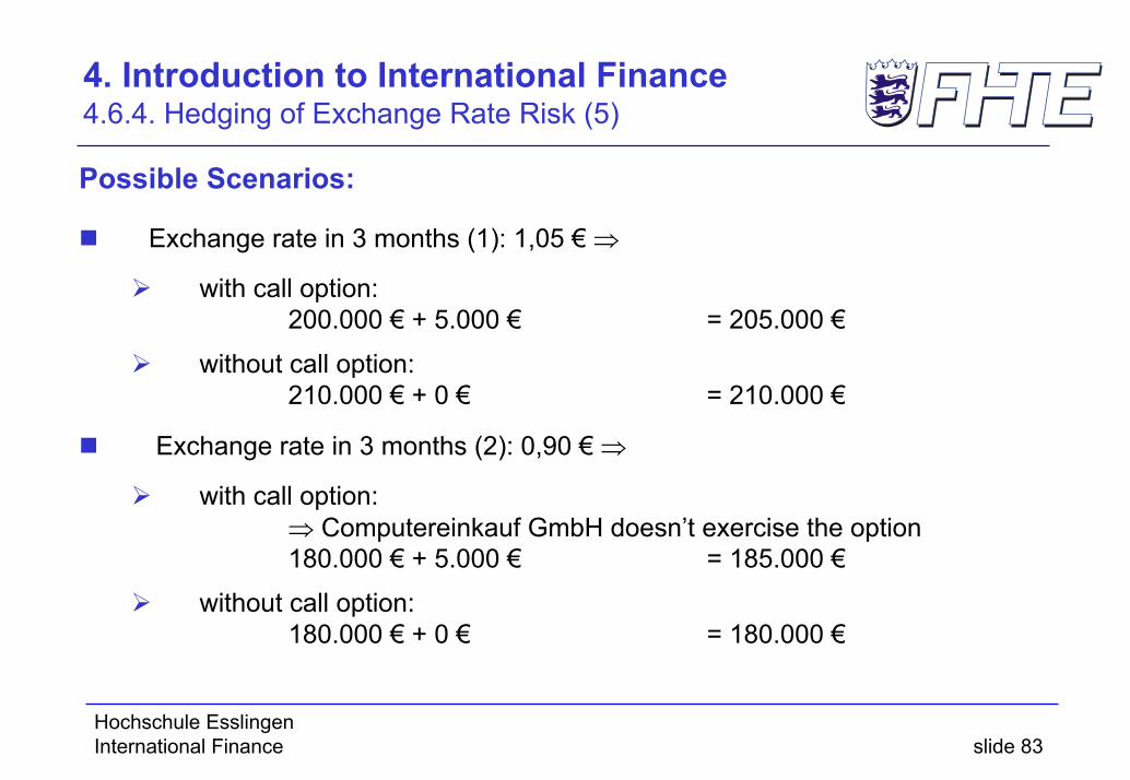
Possible Scenarios:
Exchange rate in 3 months (1): 1,05 € ⇒
with call option:200.000 € + 5.000 € = 205.000 €
without call option:210.000 € + 0 € = 210.000 €
Exchange rate in 3 months (2): 0,90 € ⇒
with call option:⇒ Computereinkauf GmbH doesn’t exercise the option180.000 € + 5.000 € = 185.000 €
without call option:180.000 € + 0 € = 180.000 €

Hochschule EsslingenInternational Finance slide 84
4. Introduction to International Finance 4.6.4. Hedging of Exchange Rate Risk (6)
Hedging with Option Contracts
spot rate
exchange rate1 €
Investment in €
200.000 call price