introduction to information retrieval today’s topic latent semantic indexing term-document...
TRANSCRIPT
Introduction to Information RetrievalIntroduction to Information Retrieval
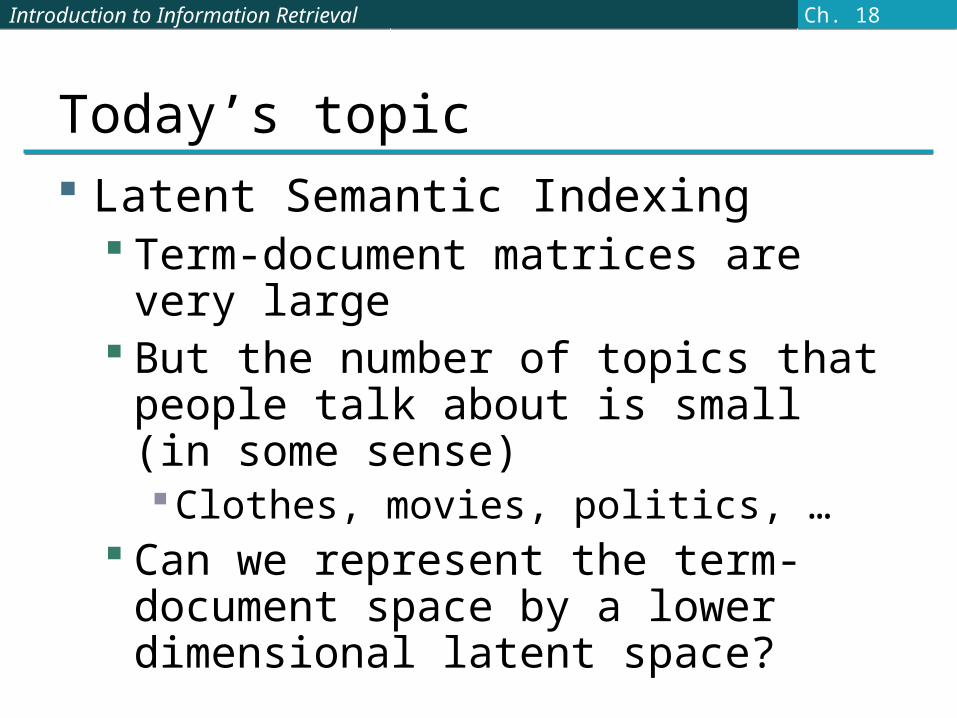
Today’s topic Latent Semantic Indexing
Term-document matrices are very large But the number of topics that people talk
about is small (in some sense)Clothes, movies, politics, …
Can we represent the term-document space by a lower dimensional latent space?
Ch. 18

Introduction to Information RetrievalIntroduction to Information Retrieval
Linear Algebra Background

Introduction to Information RetrievalIntroduction to Information Retrieval
Eigenvalues & Eigenvectors Eigenvectors (for a square mm matrix S)
How many eigenvalues are there at most?
only has a non-zero solution if
This is a mth order equation in λ which can have at most m distinct solutions (roots of the characteristic polynomial) – can be complex even though S is real.
eigenvalue(right) eigenvector
Example
Sec. 18.1

Introduction to Information RetrievalIntroduction to Information Retrieval
Matrix-vector multiplication
S 30 0 0
0 20 0
0 0 1
has eigenvalues 30, 20, 1 withcorresponding eigenvectors
0
0
1
1v
0
1
0
2v
1
0
0
3v
On each eigenvector, S acts as a multiple of the identitymatrix: but as a different multiple on each.
Any vector (say x= ) can be viewed as a combination ofthe eigenvectors: x = 2v1 + 4v2 + 6v3
6
4
2
Sec. 18.1
Introduction to Information RetrievalIntroduction to Information Retrieval
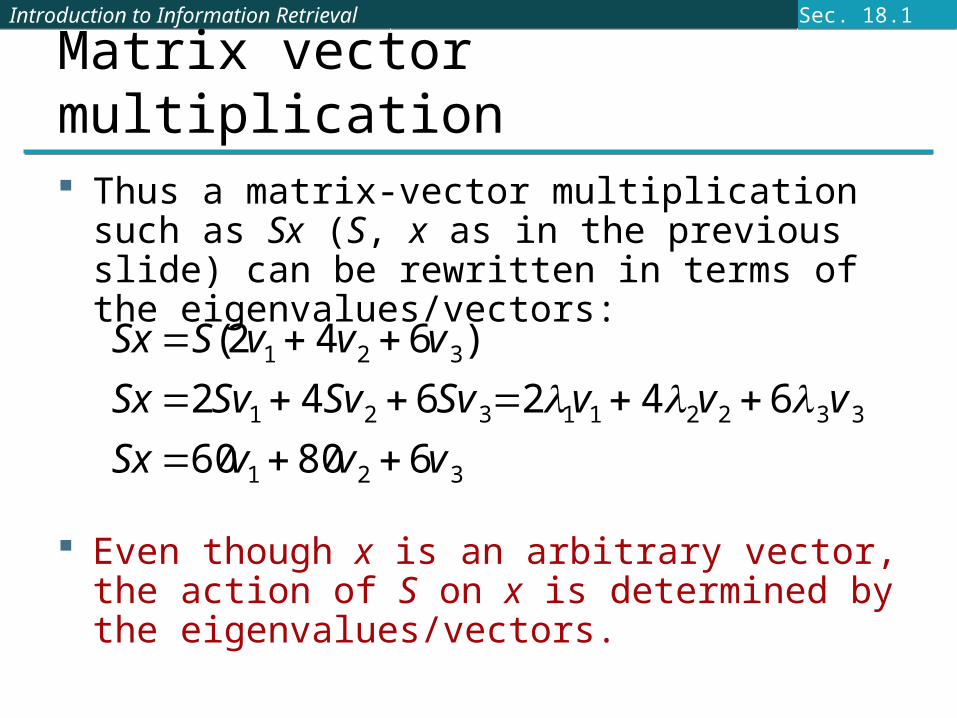
Matrix vector multiplication Thus a matrix-vector multiplication such as Sx (S, x as
in the previous slide) can be rewritten in terms of the eigenvalues/vectors:
Even though x is an arbitrary vector, the action of S on x is determined by the eigenvalues/vectors.
Sx S(2v1 4v2 6v 3)
Sx 2Sv1 4Sv2 6Sv 321v1 42v2 63v 3
Sx 60v1 80v2 6v 3
Sec. 18.1

Introduction to Information RetrievalIntroduction to Information Retrieval
Matrix vector multiplication Suggestion: the effect of “small” eigenvalues is small. If we ignored the smallest eigenvalue (1), then
instead of
we would get
These vectors are similar (in cosine similarity, etc.)
60
80
6
60
80
0
Sec. 18.1

Introduction to Information RetrievalIntroduction to Information Retrieval
Eigenvalues & Eigenvectors
0 and , 2121}2,1{}2,1{}2,1{ vvvSv
For symmetric matrices, eigenvectors for distincteigenvalues are orthogonal
TSS and 0 if ,complex for IS
All eigenvalues of a real symmetric matrix are real.
0vSv if then ,0, Swww Tn
All eigenvalues of a positive semidefinite matrixare non-negative
Sec. 18.1

Introduction to Information RetrievalIntroduction to Information Retrieval
Plug in these values and solve for eigenvectors.
Example Let
Then
The eigenvalues are 1 and 3 (nonnegative, real). The eigenvectors are orthogonal (and real):
21
12S
.01)2(||
21
12
2
IS
IS
1
1
1
1
Real, symmetric.
Sec. 18.1

Introduction to Information RetrievalIntroduction to Information Retrieval
Let be a square matrix with m linearly independent eigenvectors (a “non-defective” matrix)
Theorem: Exists an eigen decomposition
(cf. matrix diagonalization theorem)
Columns of U are eigenvectors of S Diagonal elements of are eigenvalues of
Eigen/diagonal Decomposition
diagonalUnique
for distinct eigen-values
Sec. 18.1
Introduction to Information RetrievalIntroduction to Information Retrieval
Diagonal decomposition: why/how
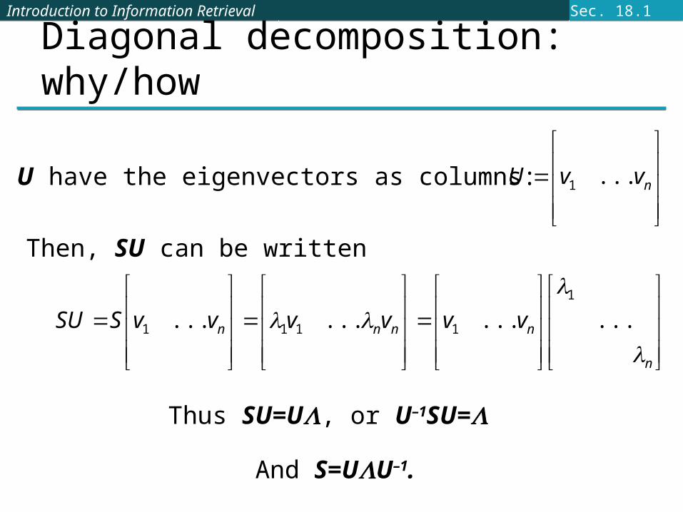
nvvU ...1Let U have the eigenvectors as columns:
n
nnnn vvvvvvSSU
............
1
1111
Then, SU can be written
And S=UU–1.
Thus SU=U, or U–1SU=
Sec. 18.1

Introduction to Information RetrievalIntroduction to Information Retrieval
Diagonal decomposition - example
Recall .3,1;21
1221
S
The eigenvectors and form
1
1
1
1
11
11U
Inverting, we have
2/12/1
2/12/11U
Then, S=UU–1 =
2/12/1
2/12/1
30
01
11
11
RecallUU–1 =1.
Sec. 18.1

Introduction to Information RetrievalIntroduction to Information Retrieval
Example continued
Let’s divide U (and multiply U–1) by 2
2/12/1
2/12/1
30
01
2/12/1
2/12/1Then, S=
Q (Q-1= QT )
Why? Stay tuned …
Sec. 18.1
Introduction to Information RetrievalIntroduction to Information Retrieval
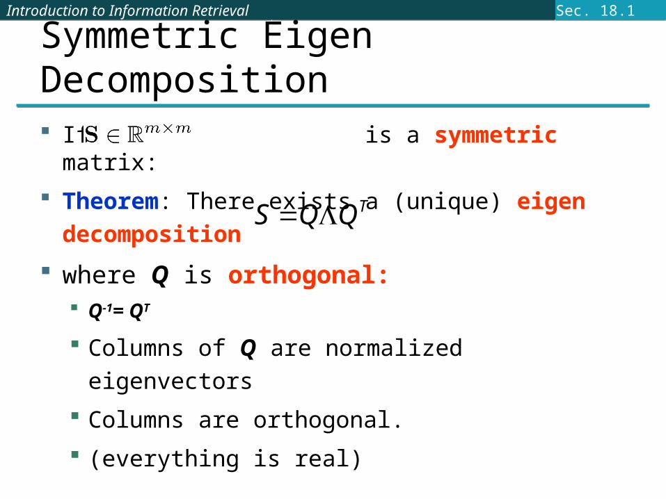
If is a symmetric matrix: Theorem: There exists a (unique) eigen
decomposition
where Q is orthogonal: Q-1= QT
Columns of Q are normalized eigenvectors Columns are orthogonal. (everything is real)
Symmetric Eigen Decomposition
TQQS
Sec. 18.1

Introduction to Information RetrievalIntroduction to Information Retrieval
Exercise Examine the symmetric eigen decomposition, if any,
for each of the following matrices:
01
10
01
10
32
21
42
22
Sec. 18.1

Introduction to Information RetrievalIntroduction to Information Retrieval
Time out! I came to this class to learn about text retrieval and
mining, not have my linear algebra past dredged up again … But if you want to dredge, Strang’s Applied Mathematics is
a good place to start. What do these matrices have to do with text? Recall M N term-document matrices … But everything so far needs square matrices – so …
Introduction to Information RetrievalIntroduction to Information Retrieval
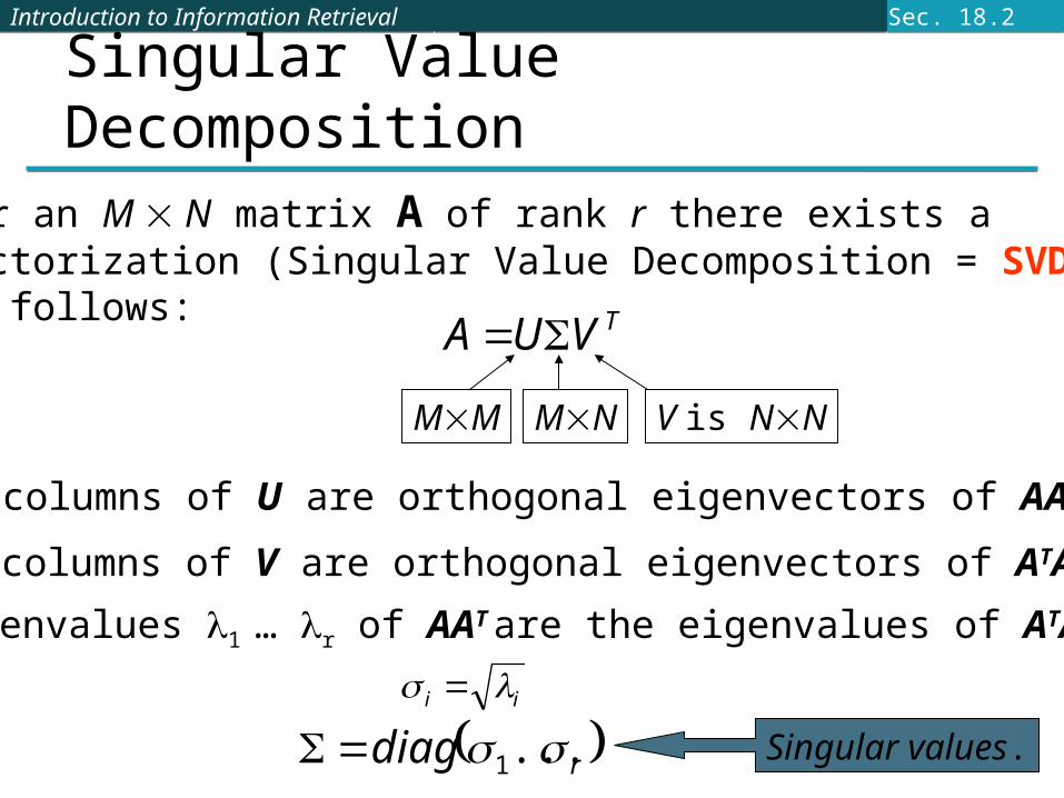
Singular Value Decomposition
TVUA
MM MN V is NN
For an M N matrix A of rank r there exists afactorization (Singular Value Decomposition = SVD)as follows:
The columns of U are orthogonal eigenvectors of AAT.
The columns of V are orthogonal eigenvectors of ATA.
ii
rdiag ...1 Singular values.
Eigenvalues 1 … r of AAT are the eigenvalues of ATA.
Sec. 18.2
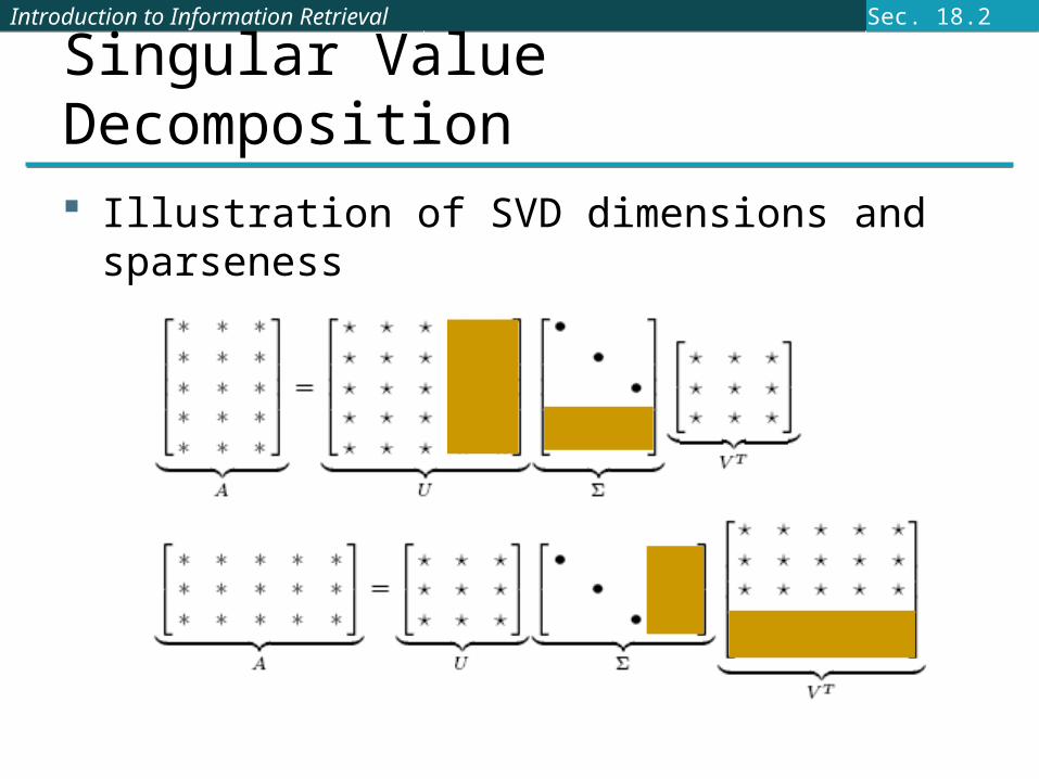
Introduction to Information RetrievalIntroduction to Information Retrieval
Singular Value Decomposition Illustration of SVD dimensions and sparseness
Sec. 18.2
Introduction to Information RetrievalIntroduction to Information Retrieval
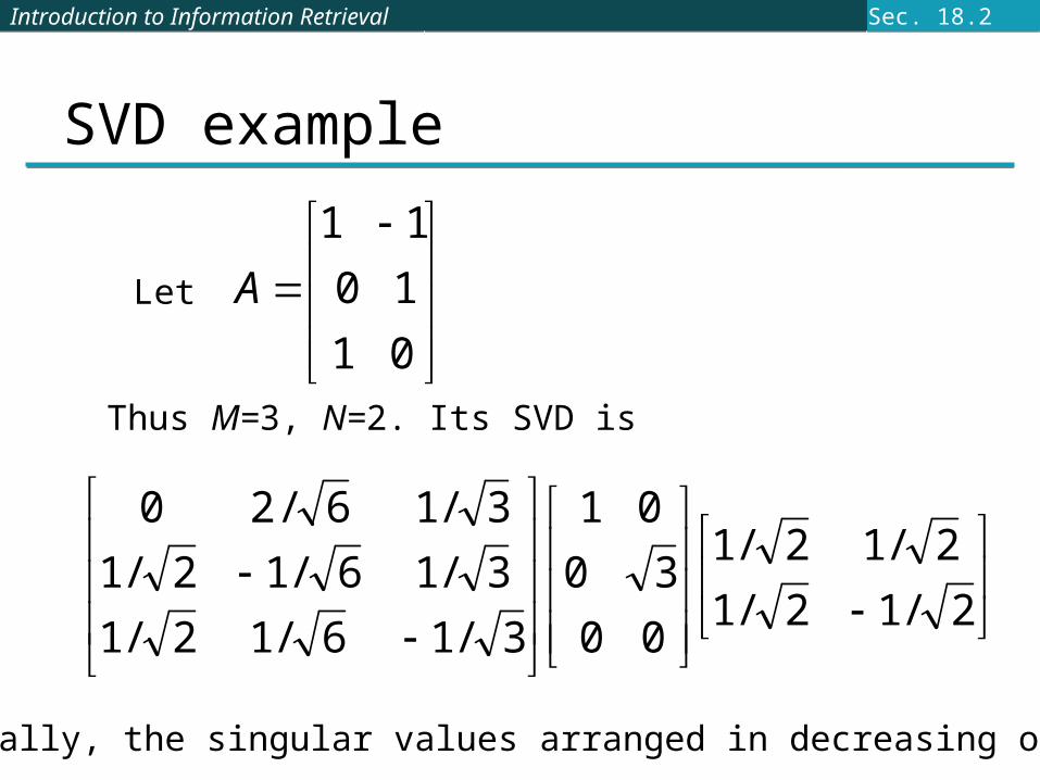
SVD example
Let
01
10
11
A
Thus M=3, N=2. Its SVD is
2/12/1
2/12/1
00
30
01
3/16/12/1
3/16/12/1
3/16/20
Typically, the singular values arranged in decreasing order.
Sec. 18.2
Introduction to Information RetrievalIntroduction to Information Retrieval
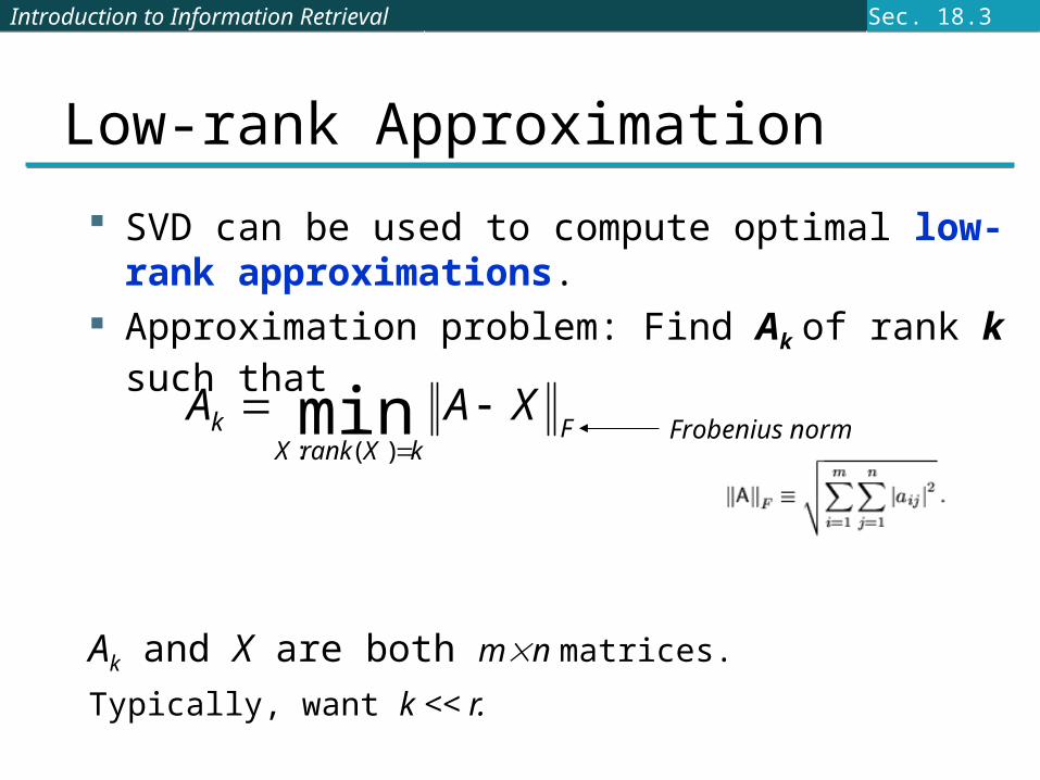
SVD can be used to compute optimal low-rank approximations.
Approximation problem: Find Ak of rank k such that
Ak and X are both mn matrices.
Typically, want k << r.
Low-rank Approximation
Frobenius normFkXrankX
k XAA
min)(:
Sec. 18.3
Introduction to Information RetrievalIntroduction to Information Retrieval
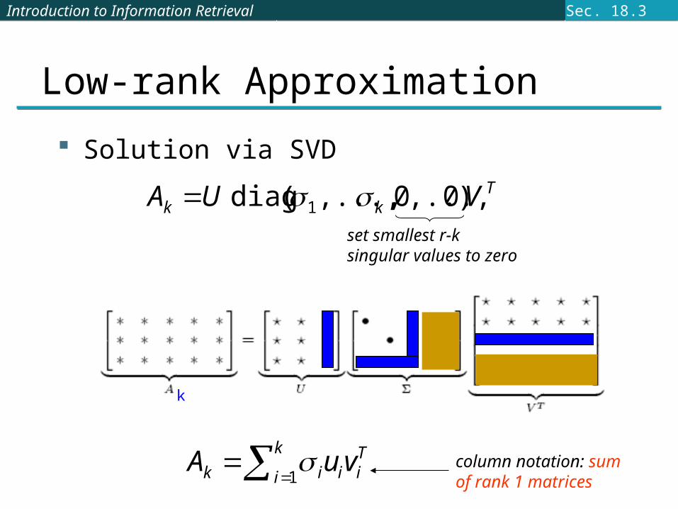
Solution via SVD
Low-rank Approximation
set smallest r-ksingular values to zero
Tkk VUA )0,...,0,,...,(diag 1
column notation: sum of rank 1 matrices
Tii
k
i ik vuA
1
k
Sec. 18.3

Introduction to Information RetrievalIntroduction to Information Retrieval
If we retain only k singular values, and set the rest to 0, then we don’t need the matrix parts in brown
Then Σ is k×k, U is M×k, VT is k×N, and Ak is M×N This is referred to as the reduced SVD It is the convenient (space-saving) and usual form for
computational applications It’s what Matlab gives you
Reduced SVD
k
Sec. 18.3
Introduction to Information RetrievalIntroduction to Information Retrieval
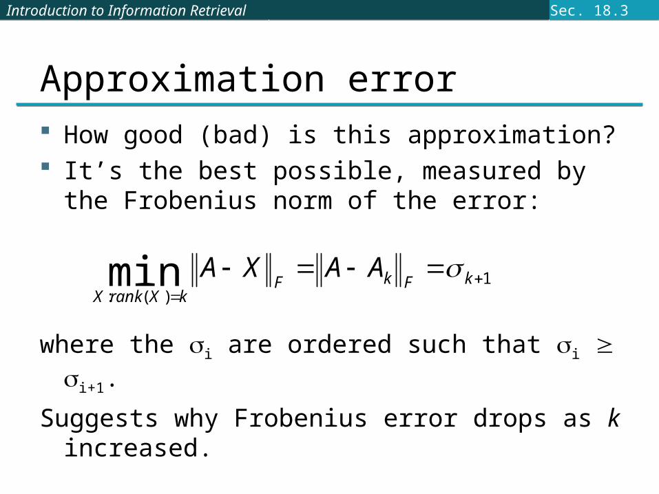
Approximation error How good (bad) is this approximation? It’s the best possible, measured by the Frobenius
norm of the error:
where the i are ordered such that i i+1.
Suggests why Frobenius error drops as k increased.
1)(:
min
kFkFkXrankX
AAXA
Sec. 18.3

Introduction to Information RetrievalIntroduction to Information Retrieval
SVD Low-rank approximation Whereas the term-doc matrix A may have M=50000,
N=10 million (and rank close to 50000) We can construct an approximation A100 with rank
100. Of all rank 100 matrices, it would have the lowest
Frobenius error. Great … but why would we?? Answer: Latent Semantic Indexing
C. Eckart, G. Young, The approximation of a matrix by another of lower rank. Psychometrika, 1, 211-218, 1936.
Sec. 18.3
Introduction to Information RetrievalIntroduction to Information Retrieval
Latent Semantic Indexing via the SVD

Introduction to Information RetrievalIntroduction to Information Retrieval
What it is From term-doc matrix A, we compute the
approximation Ak.
There is a row for each term and a column for each doc in Ak
Thus docs live in a space of k<<r dimensions These dimensions are not the original axes
But why?
Sec. 18.4

Introduction to Information RetrievalIntroduction to Information Retrieval
Vector Space Model: Pros Automatic selection of index terms Partial matching of queries and documents (dealing
with the case where no document contains all search terms) Ranking according to similarity score (dealing with large
result sets) Term weighting schemes (improves retrieval performance) Various extensions
Document clustering Relevance feedback (modifying query vector)
Geometric foundation
Introduction to Information RetrievalIntroduction to Information Retrieval
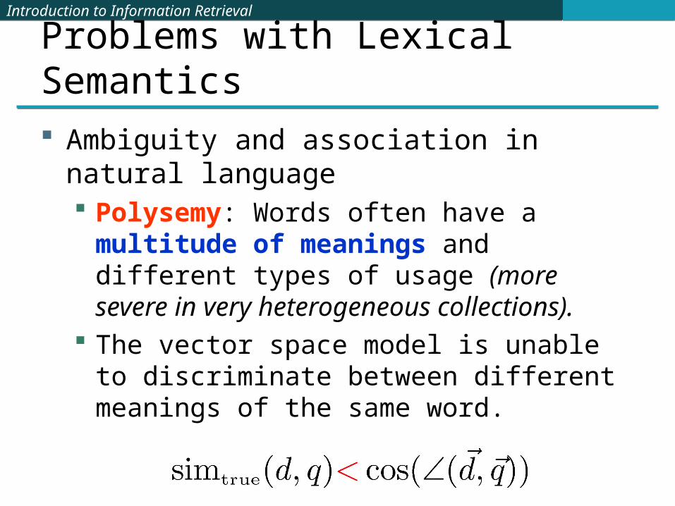
Problems with Lexical Semantics Ambiguity and association in natural language
Polysemy: Words often have a multitude of meanings and different types of usage (more severe in very heterogeneous collections).
The vector space model is unable to discriminate between different meanings of the same word.

Introduction to Information RetrievalIntroduction to Information Retrieval
Problems with Lexical Semantics Synonymy: Different terms may have an
dentical or a similar meaning (weaker: words indicating the same topic).
No associations between words are made in the vector space representation.

Introduction to Information RetrievalIntroduction to Information Retrieval
Polysemy and Context Document similarity on single word level: polysemy
and context
carcompany
•••dodgeford
meaning 2
ringjupiter
•••space
voyagermeaning 1…
saturn...
…planet
...
contribution to similarity, if used in 1st meaning, but not if in 2nd
Introduction to Information RetrievalIntroduction to Information Retrieval
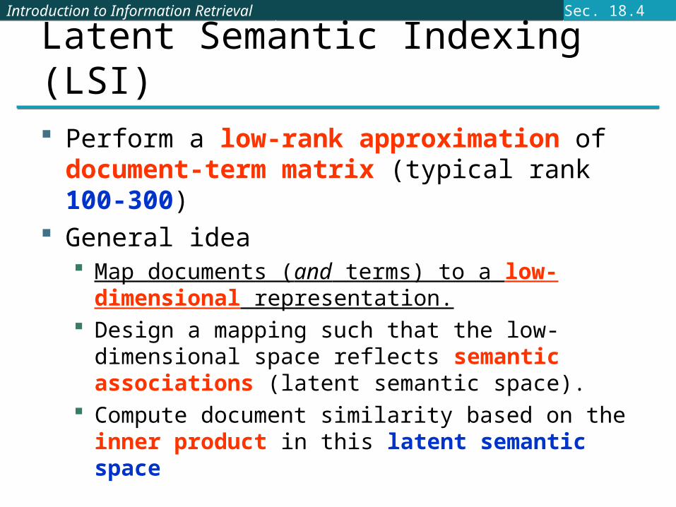
Latent Semantic Indexing (LSI) Perform a low-rank approximation of document-
term matrix (typical rank 100-300) General idea
Map documents (and terms) to a low-dimensional representation.
Design a mapping such that the low-dimensional space reflects semantic associations (latent semantic space).
Compute document similarity based on the inner product in this latent semantic space
Sec. 18.4
Introduction to Information RetrievalIntroduction to Information Retrieval
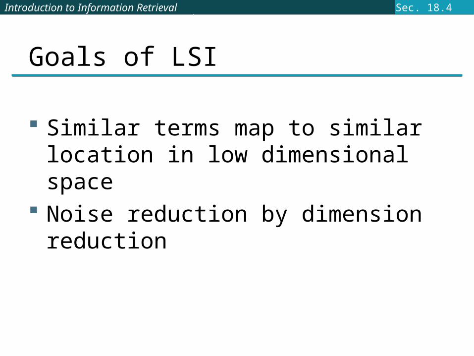
Goals of LSI
Similar terms map to similar location in low dimensional space
Noise reduction by dimension reduction
Sec. 18.4

Introduction to Information RetrievalIntroduction to Information Retrieval
Latent Semantic Analysis Latent semantic space: illustrating example
courtesy of Susan Dumais
Sec. 18.4
Introduction to Information RetrievalIntroduction to Information Retrieval
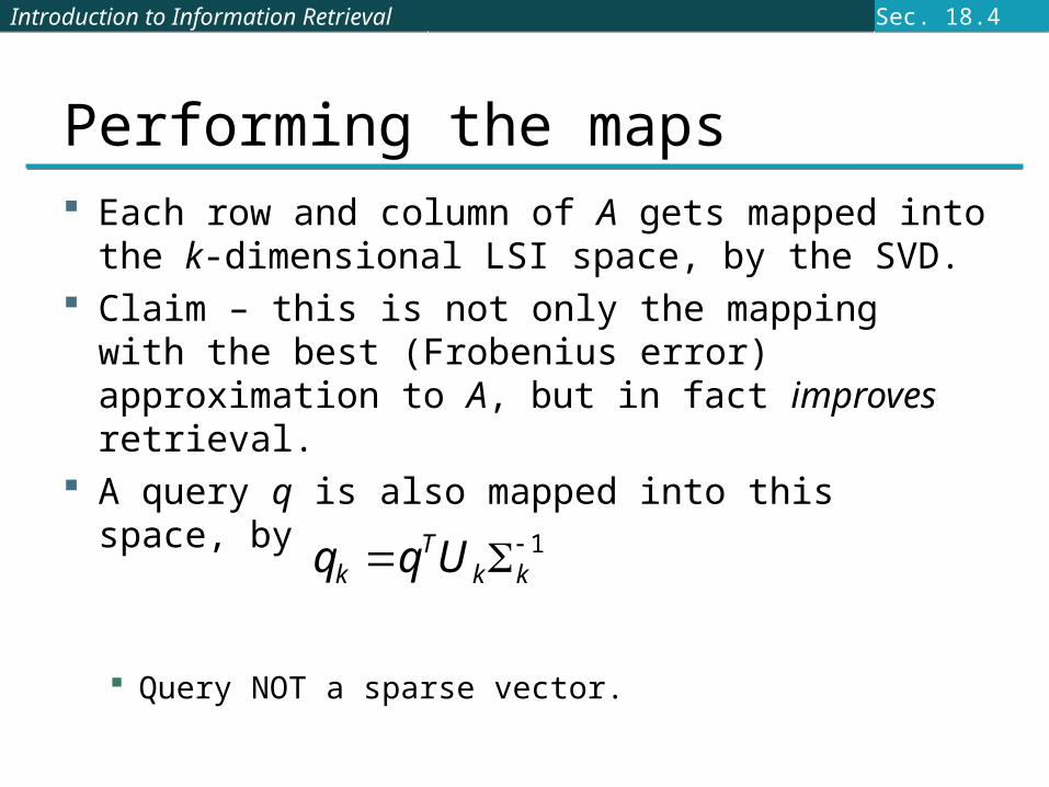
Performing the maps Each row and column of A gets mapped into the k-
dimensional LSI space, by the SVD. Claim – this is not only the mapping with the best
(Frobenius error) approximation to A, but in fact improves retrieval.
A query q is also mapped into this space, by
Query NOT a sparse vector.
1 kkT
k Uqq
Sec. 18.4

Introduction to Information RetrievalIntroduction to Information Retrieval
Empirical evidence Experiments on TREC 1/2/3 – Dumais Lanczos SVD code (available on netlib) due to
Berry used in these expts Running times of ~ one day on tens of thousands
of docs [still an obstacle to use] Dimensions – various values 250-350 reported.
Reducing k improves recall. (Under 200 reported unsatisfactory)
Generally expect recall to improve – what about precision?
Sec. 18.4

Introduction to Information RetrievalIntroduction to Information Retrieval
Empirical evidence Precision at or above median TREC precision
Top scorer on almost 20% of TREC topics Slightly better on average than straight vector
spaces Effect of dimensionality:
Dimensions Precision
250 0.367
300 0.371
346 0.374
Sec. 18.4
Introduction to Information RetrievalIntroduction to Information Retrieval
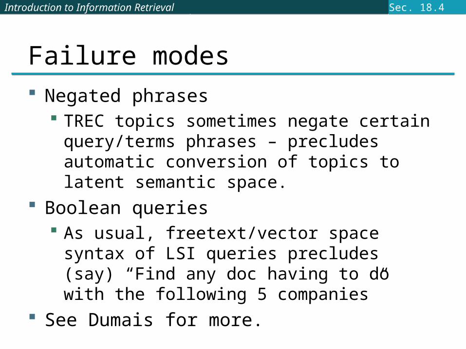
Failure modes Negated phrases
TREC topics sometimes negate certain query/terms phrases – precludes automatic conversion of topics to latent semantic space.
Boolean queries As usual, freetext/vector space syntax of LSI
queries precludes (say) “Find any doc having to do with the following 5 companies”
See Dumais for more.
Sec. 18.4

Introduction to Information RetrievalIntroduction to Information Retrieval
But why is this clustering? We’ve talked about docs, queries, retrieval
and precision here. What does this have to do with clustering? Intuition: Dimension reduction through LSI
brings together “related” axes in the vector space.
Sec. 18.4
Introduction to Information RetrievalIntroduction to Information Retrieval
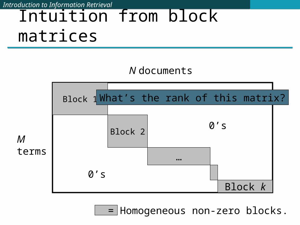
Intuition from block matrices
Block 1
Block 2
…
Block k0’s
0’s
= Homogeneous non-zero blocks.
Mterms
N documents
What’s the rank of this matrix?

Introduction to Information RetrievalIntroduction to Information Retrieval
Intuition from block matrices
Block 1
Block 2
…
Block k0’s
0’sMterms
N documents
Vocabulary partitioned into k topics (clusters); each doc discusses only one topic.
Introduction to Information RetrievalIntroduction to Information Retrieval
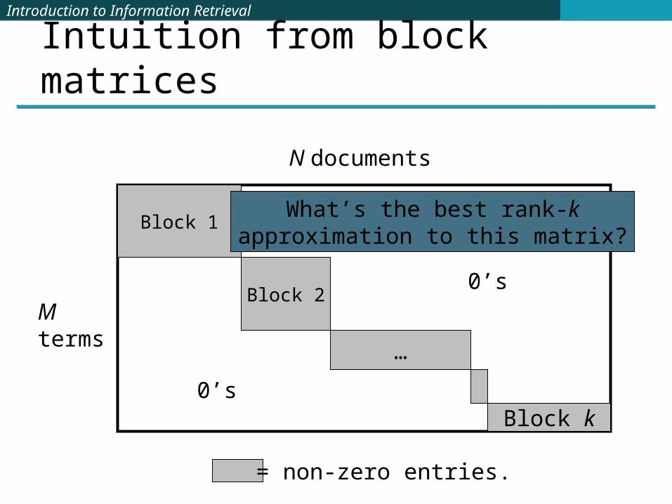
Intuition from block matrices
Block 1
Block 2
…
Block k0’s
0’s
= non-zero entries.
Mterms
N documents
What’s the best rank-kapproximation to this matrix?
Introduction to Information RetrievalIntroduction to Information Retrieval
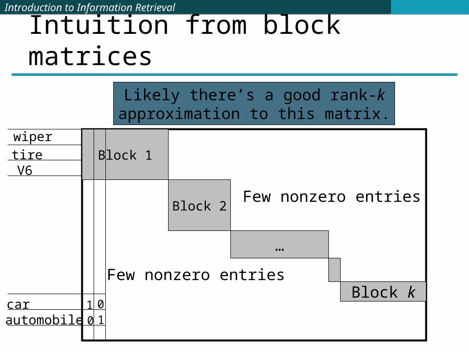
Intuition from block matrices
Block 1
Block 2
…
Block kFew nonzero entries
Few nonzero entries
wipertireV6
carautomobile
110
0
Likely there’s a good rank-kapproximation to this matrix.
Introduction to Information RetrievalIntroduction to Information Retrieval
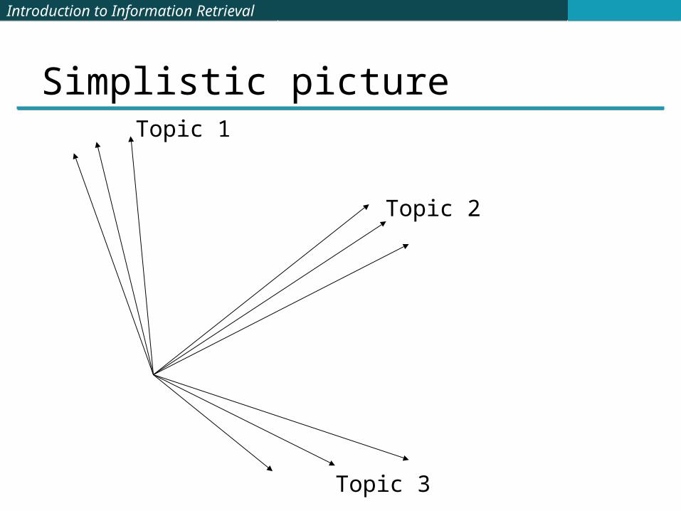
Simplistic pictureTopic 1
Topic 2
Topic 3

Introduction to Information RetrievalIntroduction to Information Retrieval
Some wild extrapolation The “dimensionality” of a corpus is the
number of distinct topics represented in it. More mathematical wild extrapolation:
if A has a rank k approximation of low Frobenius error, then there are no more than k distinct topics in the corpus.
Introduction to Information RetrievalIntroduction to Information Retrieval
LSI has many other applications In many settings in pattern recognition and retrieval,
we have a feature-object matrix. For text, the terms are features and the docs are objects. Could be opinions and users … This matrix may be redundant in dimensionality. Can work with low-rank approximation. If entries are missing (e.g., users’ opinions), can recover if
dimensionality is low. Powerful general analytical technique
Close, principled analog to clustering methods.