introduction to geostatistics - wur

INTRODUCTION TO GEOSTATISTICS

Introduction to Geostatistics

A. Stein

ÜMlIOTEEEK

4 FEB 2003

February 1999 \ ' ,N . , ^

Preface

The course element Introduction to Geostatistics gives an introduction to:

I) methods for analyzing spatial variability patterns, e.g. the definition, models and estimation

of the parameters of semivariograms;

ii) optimal prediction (kriging) and optimal interpolation;

iii) statistical sampling schemes.

The text is intended to be used by students from the Soil, Water and Atmosphere course of the

Wageningen Agricultural University, but may be used by anyone dealing with spatially

distributed data. In particular, it is written in English to allow use by Msc students. The text

consists of theoretical parts, to define and derive geostatistical concepts, and of practical case

studies as illustrations and applications. Exercises of various degrees of difficulty have been

included. A number of exercises has to be made with a personal computer. For this purpose, data

bases and computer programs are available. The examples all originate from studies in soil

science and the environment.

Prerequisites for following this course element are knowledge of soil data, and insight

into linear regression procedures.

The objectives of this course element may be formulated as follows:

Objectives:

- Understanding of a quantitative analysis of spatial variation.

- Providing tools and procedures to arrive from point observations towards predictions at

unvisited locations by means of spatial interpolation (Kriging).

- Increasing insight in spatial sampling strategies.

Interpretation of the results is crucial, along with knowledge of methods, procedures and

techniques. When spatial data are to be processed, e.g. by geographical information systems, it

should be clear, after having studied this course element, where the essential merits of a quanti

tative spatial analysis of collected data are to be found and where they have to be applied. It

Introduction to Geostatistics 2

should be clear where the major spatial uncertainties of the data with regard to the procedures

are to be found and how they can be quantified.


Table of Contents

Chapter 1. Spatial variation

Chapter 2. Data along a transect

Chapter 3. Planar data

Chapter 4. Stratification

Chapter 5. Prediction and Kriging

Chapter 6. Spatial interpolation

Chapter 7. Sampling strategies

Appendices

Suggestions for further reading

Semivariogram models

Glossary

5

8

20

27

31

39

45

49

51

54

-*\ S"-££ i T / i o l^'&f' ' -/"Op


Spatial variation

Variability (Oxford: the fact of quality of being variable in some respect) in space is

defined as the phenomenon that a variable changes in space. At a certain location this variable

is observed. At a very small distance from this place the variable may be observed again, and it

will likely deviate from the previous observation. The deviations may increase when the

distances increase. Description of variability (how large are the deviations if the distance

increases) is important for a process based interpretation. When cultivating plants, when

indicating soil pollution and when interpreting the soil condition interpolation is necessary, based

on a certain assumption of stationarity. The observed variability violates this on the one hand,

but may be used on the other hand to quantify the uncertainty.

The study of variability is in principle independent of any discipline, and even from the

earth sciences (important recent developments are observed in social sciences and in

econometrics). However, especially in the earth sciences a quantitative approach using GIS and

geostatistics has fully been developed, first in mining and geology, later as well in agricultural

and environmental sciences.

Spatial data are likely to vary throughout a region. Even when all data were measured at

precisely the same manner, that is: without error and by the same surveyor, variation will occur

due to different conditions of the soil, the water or the atmosphere. When, for example, the

percentage of clay is being determined, this amount will vary from place to place. Because such

variation takes place in space, we will speak about spatial variation. Evidently, this variable (clay

content) is allocated to its place in space.

Developments in geostatistics have started in the past decades to quantitatively deal with

spatial variation. The major aims of geostatistics are to handle large sets of spatial data. The

different stages are an analysis of the (spatial) dependence, i.e. how large is the variation as a

function of the distance between observation, to produce computerized maps, to determine the

probabilities of exceeding some threshold value and to determine sampling schemes which are

Introduction to Geost3tistics 5

Chapter 1: Spatial variation

optimal in some predefined sense. The main distinction with statistics is that in geostatistics

variables are used that are linked to Locations. Some authors term such variables 'regionalized

variables' or 'geovariables'.

Many ways may be distinguished to deal with spatial variation and to use it for practical

purposes. Traditionally, choropleth maps have been constructed, like the regular soil maps,

geological maps and hydrological maps. Such maps show the main differences between

delineated areas, but to a large extent neglect the variation within the units. Depending upon the

map scale, the variation in soil and in geological and hydrological properties has been displayed.

One commonly terms the map 'small scale maps' when these display the spatial variation at a

small scale, such as 1:100,000 or 1:250,000. The maps are termed 'large scale maps' when these

display the spatial variation at a large scale, e.g. 1:25,000, or 1:10,000. The compilation of such

a map is outside the scope of this course. We will use original point data instead. The soil map,

however, will be used in several exercises, being in many applied studies one of the major

sources of available prior information. The spatial variation will mainly be studied for areas

within units. Moreover, delineated soil areas may not be of primary importance when one is

studying and interpreting spatial variability of the individual spatial variables. For example: the

distribution of a pollutant may not be associated with distinguished soil units.

Statistical and geostatistical procedures may be helpful in a number of stages of

interpreting and evaluating data with a spatial distribution. In many studies they have proven to

be indispensable, especially when the number of available data increases. Without having the

intention to being complete, one may think of the following aspects:

1. The type and the amount of the variation. Some examples are: which property varies

within a region? Is every property varying at the same scale? What is the relation between

spatial variation of a property and aspects of soils like sedimentation, development and

human influences in the past? Is there any relation between spatial variation of, say, soil

variables and hydrological and botanical data?

2. To predict the value of a variable at an unvisited location. Some examples: what is the

mean value of nitrate leaching in a parcel? What is the total amount of polluted soil?



What is the uncertainty associated with the prediction? Are predictions easily being

combined to create a map of an area?

3. To determine probabilities that a pollutant exceeds an environmental threshold level. Can

it be stated that an area is not polluted with a probability of 98%?

4. To develop a sampling scheme. Typical questions include: how many observations does

one need? Which configuration of the data is most appropriate given the objective of a

particular inventarization study?

5. To use the data in model calculations, for example to calculate the water restricted yield

of a particular crop, or to calculate the amount of pesticide leaching to the ground-water.

The role of spatial variation is: what is the impact of spatial variation for variation in the

model calculations? How sensitive is the model to variation in the input parameters?

How much spatial variation is observed in the output variable?

We will have no opportunity to deal with all the questions at a similar level of detail. It

should be clear, that a quantitative approach to spatial variability is of a crucial importance in

many soil scientific studies.

In this course we will focus our attention entirely on the analysis of single properties,

collected along a transect or in a plane. The analysis of multivariate properties is postponed to

another course, 'Statistical mapping aspects' (Corsten, Stein and Van Eijnsbergen, 1990). The

analysis of three-dimensional data is treated in the literature (Journel and Huijbregts, 1978;

Ripley, 1981).



Data along a transect

In this chapter spatial variation occurring along a transect will be studied.

Imagine that n measurements on a single variable are collected along a transect, that is

a line in the field. We could think about the clay content, the thickness of a specific horizon, the

depth to ground-water, the amount of precipitation along a line orthogonal to a mountain range,

the amount of Cadmium and Organic Carbon, etc. We could display these data in a graph as

Clay contents for two horizons

Coordinate [m]

follows:

Apparently, n -7 observations are taken at equal distances from each other. Along the

horizontal axis the coordinate along the transect is given, measured in metres from an arbitrary

origin and denoted by xj through X7. Maybe the observations are just local deviations from a

general mean. This will be the approach followed in geostatistics. All observations will be

considered to deviate from the mean m. But if one observation deviates in one direction, say:

higher than the mean, than observations close to this observation are likely to deviate in the same



direction. Uncertain here are the terms 'close to' and 'likely'. We will study now how to quantify

these concepts. It takes us to defining spatial dependence.

Dependence

Observations in space are linked to their coordinates and each observation has its own

specific place in space. The value of the coordinate (x) is essentially linked with the variable Y.

Such sj^atial^ariables are therefore denoted with Y(x): the place dependence of the variable Y.on

the location x is given explicitly. They are termed regionalized variables. For Y(x) one may read

any spatially varying property. The variable Y(x) is put in capitals to indicate that it is a stochastic

variable, subject to random influences.

One important characteristic to deal with is that the data close to each other are more

likely to be similar than data collected at larger distances from each other. This implies that the

variables Y(xi) and Ffej in two locations xi and xj are probably more alike if the distance

between the locations is small, than if the distance is large. The dependence between regionalized

variables at different locations is the main characteristic difference from traditional stochastic

variables and the size and the functional form of the differences as a function of the distance will

be studied.

An important aspect of regionalized variables is their expectation E[Y(x)] - \i and their

variance Var[Y(x)] = a2. There exist situations, however, where pi does not exist, or a2 is not

finite . In geostatistics attention will be restricted to the less restrictive requirement, summarized

in the so-called intrinsic hypothesis (Journel & Huijbregts, 1978). Consider two points along the

transect: x and x+h, the latter point being located at a distance h from the first point x. The

intrinsic hypotheses is:

i) E[Y(x) - Y(x+h)] = 0

ii) Var[y(x) - y(x+h)] < °° and is independent of x.

A famous example is the so-called Brownian motion. Particles in a fluid move extremely irregularly. When the values of the coordinates are of one of these particles are observed a single realization Y(x) is obtained. It is well known (cf. Cressie, 1991) that E[Y(x)] = 0, but that Var[Y(x) - Y(x)] = \h\, implying that Var[Y(x)] does not exist.



The first part can be interpreted as follows: the expectation of the difference of a

regionalized variable at location x and at a distance h from x equals zero. To put it differently:

expectation and variance are translation invariant, implying that there is no trend (sometimes

called: drift) in the region. The second part of the hypothesis requires that the variance of the

difference of a regionalized variable measured at location x and at a distance h from x exists, and

is independent of x. The difference between the two variables Y(x) and Y(x+h) is called a pair

difference. The precise form of the dependence of the variance of pair differences on h is often

interesting for interpretive purposes, as we will see below.

The spatial dependgnce function of observations is defined by the second part of the

intrinsic hypothesis. It is termed the semivariogram y(h). The semivariogram is defined as a

y (%) Ï Wn "<•'*<,c*- <s~~ ï(h) = i E \Y(x)-Y(x + h)]

function of the distance h between locations in the observation space:

Because the expectation of Y(x)-Y(x+h) is equal to zero (intrinsic hypoethis!), the semivariogram

equals half the variance of pair differences at a distance h. Due to the assumption summarized

in the intrinsic hypothesis this variance of pair differences exists and is properly defined. Notice

the inclusion of the factor '/SUP the expression, due to allow a straightforward comparison with

the covariance function: j{h) = C(0) - C(h).

Remarks __

1. The semivariogram is independent of the place where the regionalized variables are located.

The squared pair differences have the same expectation, regardless whether they are

measured at one part of the transect or at another part of the transect. Loosely speaking,

we expect similar differences between observations independent of the part in the area.

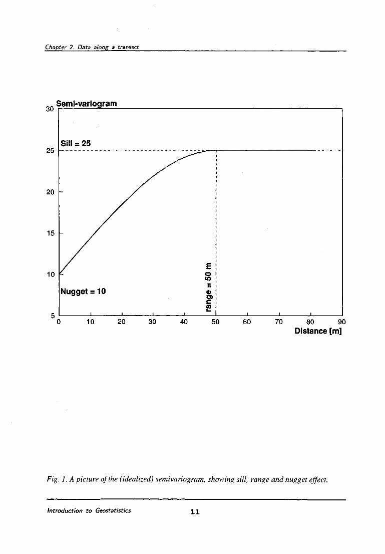
2. In many practical studies one observes an increase of the semivariogram with increasing

distance between the observation locations. This implies that the dependence decreases

with increasing distance h between locations. Loosely speaking: observations close to

each other are more likely to be similar than observations at a larger distance from each

other. A general picture of the semivariogram is given in figure 1.

Introduction to Geostatistics 1 0


30 Semi-variogram

25

20

15

10

Sill = 25

Nugget = 10

o w ii o> O) c (0

10 20 30 40 50 60 70 80 90 Distance [m]

Fig. 1. A picture of the (idealized) semivariogram, showing sill, range and nugget effect.



Estimating the semivariogram

The definition of the semivariogram given above is a theoretical one. To estimate the

semivariogram in practical cases we will first pay attention to the case that n equally spaced

observations are collected (Figure 2). It is easy to show that the total number of pairs of points _

(= Np) equals Vm-in-l), a number which considerably exceeds the number of observations

themselves (for n = 2, Np = 1, for n = 10, Np = 45, for n = 100, Np = 4950, and for n = 400, Np =

79800). r ^ / " \

First consider all pairs of points with intermediate distance h equal to 1, that is all paiijs /

of successive points. The differences between the observations constituting a pair are squared, j

summed and divided by two and by the total number N(l) of pairs with intermediate distance y\~ Li

equal to 1 : \j „ -: £

J N(I)

it is easy to show that N(l) equals (n-1) (exercise!).

Next, an estimate for the semivariogram for distance h = 2 is found by taking all pairs of

points with intermediate distance 2. Again, the differences between the observations constituting

a pair are squared and summed, and are divided by two and by the total number N(2) of pairs with

intermediate distance equal to 2:

J N(2)

The number N(2) equals n-2. This procedure is repeated for all the other distances involved. By

means of this procedure pairs of distances and estimated semivariogram values ( l ,f(l)) , (2,

7(2) ), (3, f(3) ), .... are obtained. These may be displayed in the form of a graph, giving the

estimated semivariogram f(h) as a function of the distance h (= 1,2,3,...).

Exercise Consider the following clay content observations collected at equal distances (say lm) along a transect: 15, 20, 18, 25, 28, 22. Estimate semivariogram values for the distances h = lm, h - 2m and h = 3m.



If the distances between the observation locations (the sampling distance) are not equal

to each other, distance classes are created: all pairs of points with approximately the same

sampling distance are grouped into one distance class. This distance defines the class to which

the pair belongs.

As an example of distance classes consider data which are irregularly spaced, with

sampling distances approximately equal to 1 m. The first distance class is the class of all

points with an intermediate distance between 0.5m and J.5m. To this class each pair of

observations with a sampling distances between 0.5 m and 1.5m is allocated. However,

a pair of observations with a sampling distance of 1.6m, or of 0.3m is assigned to

another class. The average distance for the pairs of observations assigned to the 1m-

class is approximately equal to 1m. The next distance class contains all the points with

intermediate distances between 1.5m and 2.5m, with average distance approximately

equal to 2m, etc. In some programs (as in SPATANAL) there is a small distance class

which precedes the first distance class and contains all pairs of points with intermediate

distance less than one half of the lag length.

The user usually has to decide upon a lag length. Sometimes this choice is rather obvious,

as in the example of the equi-distant observations. A choice for a lag length typically influences

the number of distance classes. If the lag length is chosen to be large (larger than the largest

occurring distance) only one distance class remains that contains all pair of observations. The

estimated semivariogram value % for this distance class equals the estimated variance of the

variable: the spatial dependence between the observations is then neglected. At the other extreme

we may choose a very small lag length, resulting in a large number of distance classes, each

containing only a few pairs of observations. Although this may be illustrative for some purposes,

it is usually not very informative.

For all practical purposes there are some general rules which have to be obeyed in order

|__to obtain reliable semivariogram estimates:

1. The number of pairs of observation points in each class must exceed 30.



mg/kg mg/kg

mg/kg mg/kg

100

Coordinate [m]

100

Coordinate [m]

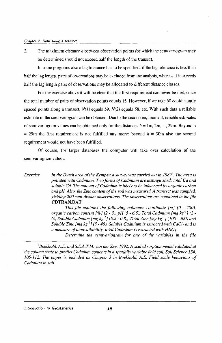
Fig. 2. The transect data collected in the Kempen area.



2. The maximum distance h between observation points for which the semivariogram may

be determined should not exceed half the length of the transect.

In some programs also a lag tolerance has to be specified: if the lag tolerance is less than

half the lag length, pairs of observations may be excluded from the analysis, whereas if it exceeds

half the lag length pairs of observations may be allocated to different distance classes.

For the exercise above it will be clear that the first requirement can never be met, since

the total number of pairs of observation points equals 15. However, if we take 60 equidistantly

spaced points along a transect, N(l) equals 59, N(2) equals 58, etc. With such data a reliable

estimate of the semivariogram can be obtained. Due to the second requirement, reliable estimates

of semivariogram values can be obtained only for the distances h = lm, 2m,..., 29m. Beyond h

= 29m the first requirement is not fulfilled any more; beyond h = 30m also the second

requirement would not have been fulfilled.

Of course, for larger databases the computer will take over calculation of the

semivariogram values.

Exercise In the Dutch area of the Kempen a survey was carried out in 198? . The area is polluted with Cadmium. Two forms of Cadmium are distinguished: total Cd and soluble Cd. The amount of Cadmium is likely to be influenced by organic carbon andpH. Also, the Zinc content of the soil was measured. A transect was sampled, yielding 200 equi-distant observations. The observations are contained in the file CDTRAN.DAT

This file contains the following columns: coordinate [m] (0 - 200), organic carbon content [%] (2 - 3), pH (5 - 6.5), Total Cadmium [mg kg' ] (2 -6), Soluble Cadmium [mg kg' ] (0.2 - 0.8), Total Zinc [mg kg' ] (100 - 300) and Soluble Zinc [mg kg'1] (5 - 40). Soluble Cadmium is extracted with CaCh and is a measure of bioavailability, total Cadmium is extracted with HNO3.

Determine the semivariogram for one of the variables in the file

2Boekhold, A.E. and S.E.A.T.M. van der Zee. 1992. A scaled sorption model validated at the column scale to predict Cadmium contents in a spatially variable field soil. Soil Science 154, 105-112. The paper is included as Chapter 3 in Boekhold, A.E. Field scale behaviour of Cadmium in soil.



CDTRAN.DAT. Use the program UNISPAT. - Choose a variable of interest - Specify the file column of the coordinate - Choose a lag length of 1 m - Set the number of lags equal to 100. - Give a display of the results and save it. Re-run the previous steps with a lag length of 2m, and nr. of lags equal to 50 and with a lag length of 10 m and nr. of lags equal to 10. Compare the different semi-variograms qualitatively.

Fitting a semivariogram model

It is often necessary to fit a specific_fijnction through the semivariogram estimates. A

practical way to do this is to estimate the parameters of such a function by a nonlinear regression

procedure. On behalf of positive-definiteness (to which we will return below) not all functions

one could think of are permissible. Some functions which are permissible are rarely encountered

in practice. We will restrict ourselves to the permissible models given in the Appendix, for which

the parameters can be being estimated from available data. In many practical studies,

combinations of several models are often encountered. Especially a combination of the nugget

effect model with other models is often observed, yielding a semivariogram with a discontinuity

in the origin. Several of the above functions are displayed in figure 3.

The interpretation of several parameters is as follows:

1. The sill value (or thejvaxiance) is the value which the semivariogram reaches if h tends

to infinity, i.e. if the observations are growing to be uncorrelated.

2. the range of the semivariogram is a measure for the distance up to which the spatial

dependence extends. Between locations separated by a distance exceeding b the

regionalized variables are uncorrelated, between locations separated by a distance smaller

than b the regionalized variables are dependent.

3. the nugget effect, a term borrowed from gold mining, contains the non-spatial variability.

The sources of such variability are, for example, the operator bias (i.e. two operators may

judge the same characteristic quite differently, like the clay percentage), the measurement

error (most observations are subject to some uncertainty), and the short-distance



40 Semi-variogram

30

20

10 Linear model Exponential model Spherical model Gaussian model Hole effect model

10 20 30 40 50 60 70 80 90 Distance [m]

Fig. 3. Different semi-variogram models. The corresponding euqations are included in the appendix.



variability, i.e. the variability caused by processes that pertain to distances shorter than

the smallest sampling distance (if cyanide is measured at 5m distances, the variability

assigned to its binding on iron which is highly varying in the soil, may not be accounted

for). The nugget effect does not measure a systematic deviation in the observations, such

as all measurements are shifted by a fixed constant value.

Sill value and range are not being observed in all practical situations, for which a power

model is then the most appropriate one to be used.

Whenever a sill value is reached it might be interesting to study the sill/nugget ratio,

giving an indication of the part of the variability to be assigned to spatial variability and of the

part to be assigned to non-spatial variability. If the ratio is close to 1, the non-spatial variability

is preponderant, otherwise the spatial variability is. If the ratio is close to 1, the semivariogram

is modeled with the nugggt£ffeclmodel. If this model is observed, the observations are spatially

uncorrected.

To compare different permissible variogram models, use can be made of the SSD/SST

ratio: SSD is the square sum of déviances, SST the total sum of squares. Let the n variogram

estimates (as obtained by UNISPAT) be denote by % with average value mr And let the values

of the variogram model be denoted by g,. Then

ssp_^(g;-rJ j — / 1 2

SST ,=; ( gi - mr )

If the model is close to the observed semivariogram values, then g, and )f are close to each other,

yielding a low SSD/SST ratio. However, if the g, are far from the ft they are close to my, and

hence the SSD/SST ratio is close to 1. The SSD/SST ratio may be used to compare different

models for the same collection of observed semivariogram values. However, it must not be used

to compare different values for number of lag and lag length, because it depends upon the number

of lags by the summation index.

Exercise Use the WLSFIT (Weighted Least Squares FIT) program. Determine the values of sill, range and nugget effect of the semivariogram obtained in the previous



exercise - output is saved in the file SPATx.RES, where x is the column number of the variable. Use a spherical model, an exponential model, a Gaussian model and a linear model. Make a table with values for nugget, sill, range, sill/nugget ratio and SSD/SST ratio. Which function is the best one? How would you interpret the sill/nugget ratio?

Exercise Repeat the previous exercise, but now use SPSS. First edit the SPATx.RES file, by deleting the first 7 unnecessary rows. Delete any row for which the no. of pairs of points is equal to 0. Also, change the E-format of the gamma values to Format, for example by reading the file into Lotus, and writing it back as a print file. Make an SPSS-steering file which contains the following lines:

data list file = 'c:\geostat\spat5.txt' free /vl v2 npairs dist gam.

MODEL PROGRAM cO=l a=10 b=5. COMPUTE PRED = cO + a*(l-exp(-dist/b)). NLR GAM WITH DIST.

Compare the calculations with those obtained with WLSFIT.

Remark. The above procedures work often relatively well. But some critical thoughts are relevant

at this stage: the first procedure uses a weighted fit, whereas the second uses an unweighted fit.

Also the SAS program can be applied to do a weighted non-linear fit. But more importantly,

when applied to different lag lengths and number of lags different results may be obtained. To

overcome this essential problem, Restricted Maximum Likelihood must be applied. At the

current stage, we will only apply any of the straightforward techniques just described.



Chapter 3. Planar data.

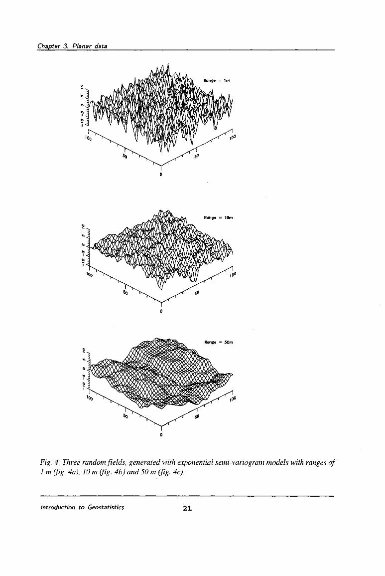
Planar data are data collected in a two-dimensional area, for example a field, a parcel, a

country, a bounded region, etc. Some examples of a variable in a two-dimensional space are

given in figure 4. The first picture shows a field with a range of 5 m, the second picture with a

range of 10 m, the third with a range of 25 m. For all fields the mean equals 0, there is no nugget

effect and the sill value equals 10. These fields are generated by means of the turning bands

method. In practice, one is seldom (if ever) able to observe a whole field entirely: one always has

a finite sample only. On the basis of this sample, properties of the population must be obtained:

the mean and the variance, but also the semivariogram, since it will not be clear from the start

whether we have to deal with a population given by figure 4a, 4b or 4c.

In order to determine the semivariogram for such data an approach similar to that for the

transect data defined above can be applied. The only complication is that to each observation an

x and ay coordinates is associated, instead of just one coordinate.

Consider an area which is homogeneous (stationary) with regard to the variable being

studied. The semivariogram y(h) is a function of the distance h between locations in the area. A

reasonable distance measure is the Euclidean distance: for any two points with coordinates (x]tyi)

and (X2J2) the squared distance h2 equals (xi-x2f + {yi-yif. Like the one-dimensional (transect)

semivariogram, the semivariogram for distance h equals half the expectation of squared

differences of variables located at this distance from each other.

An estimate f(h) may be obtained by taking for a fixed value of h all pairs of points with

an separation distance approximately equal to h, squaring the differences between the

measurements constituting such a pair, summing these squared differences and dividing the sum

by 2 and by the total number of pairs N(h) obtained for this distance. This is repeated for all

values of h. Again, a graph may be composed to display f(h) as a function of h. There are

several alternatives to estimate the variogram. One particular way, a robust estimator is

calculated as



Rangs = 1m

Fig. 4. Three random fields, generated with exponential semi-variogram models with ranges of 1 m (fig. 4a), 10 m (fig. 4b) and 50 m (fig. 4c).



N(h)

0.494 yRoh = — ' ' r . The robust variogram estimator yields good results when

0.457+ -N(h)

the data show some outliers. An observation is an outlier, when its value strongly deviates from

surrounding observations. This particular observation then has a strong influence on the

calculated variogram, if the squared differences are used. Its influence is weaker when the robust

estimator is used.

Unless there are very strong objections, one may assume isotropy, i.e. the field shows the

same spatial structure in different directions. However, in some studies the assumption of

isotropy is difficult to maintain. One then has to turn to anisotropy, e.g. variables show different

dependence structures in different directions. Anisotropy of (soil) variables occurs, for example,

if data are collected perpendicular and parallel to a river or a mountain ridge, or if the clay

percentage is sampled in a polder area having a preferential sedimentation pattern. For

anisotropic variables the spatial variation is (structurally) different for the different directions.

The study of isotropy vs. anisotropy is carried out by means of the semivariogram.

Anisotropy is displayed by recognizing that the semivariogram in one direction has another range

than in the other direction: the spatial dependence differs for different directions. In one direction

(the shorter range) larger differences are likely to be encountered than in the other direction

(longer range). \;

To calculate direction specific semivariograms direction classes are to be defined. To do

so, consider the pairs of points which are used to estimate the semi-variogram. The (imaginary)

line which connects a pair of points has a length equal to h, but also an angle a with the x-axis

(Figure 5). For example, if data are collected following a square grid, the connection lines for

many pairs of points has an angle equal to 0° with the x-axis. Also, the connection lines for many

pairs of points has an angle equal to 90° and others with angles equal to 45° and 135° with the

x-axis. When studying anisotropy, a separate semivariogram is constructed for all pairs of points

for which the connection line has a specified angle with the x-axis. For the grid data, angles of

0°, 45°, 90°, and 135° could be selected when deciding upon 4 directions of interest.



12 14

X-coordinate

Fig. 5. Direction angle (a) and direction tolerance (fi) expressed for data collected in a square grid.



However, many data are not collected as a grid. To deal with any pattern of collected

data, direction classes are formed, which contain all pairs of points for which the connection line

does not deviate more than a specified precision (say (p) from the given direction. Reasonable

values for cp could be 5°, 10°, or half the direction interval. Returning to the grid example, and

specifying a value of 9 of 10°, the 0°-class contains all pairs of points for which the angle of the

connection line with the horizontal axis equals 0° ± 10°, the 90°-class contains all pairs of points

for which the angle of the connection line with the horizontal axis equals 90° ± 10°, etc.

Some considerations governing the choice for (p are: each direction/distance class should

have sufficient pairs of points in order to properly estimate the semivariogram (therefore cp

should preferably be large); every point pair should be attributed to precisely one

direction/distance class (therefore cp should be equal to half the direction interval); the direction

tolerance should be equal to some standard uncertainty bound.

To study anisotropy a rather extensive database is needed: for each distance/direction

class sufficient pairs of points must be available. Only in a limited number of practical studies

one will be able to carry out such a study.

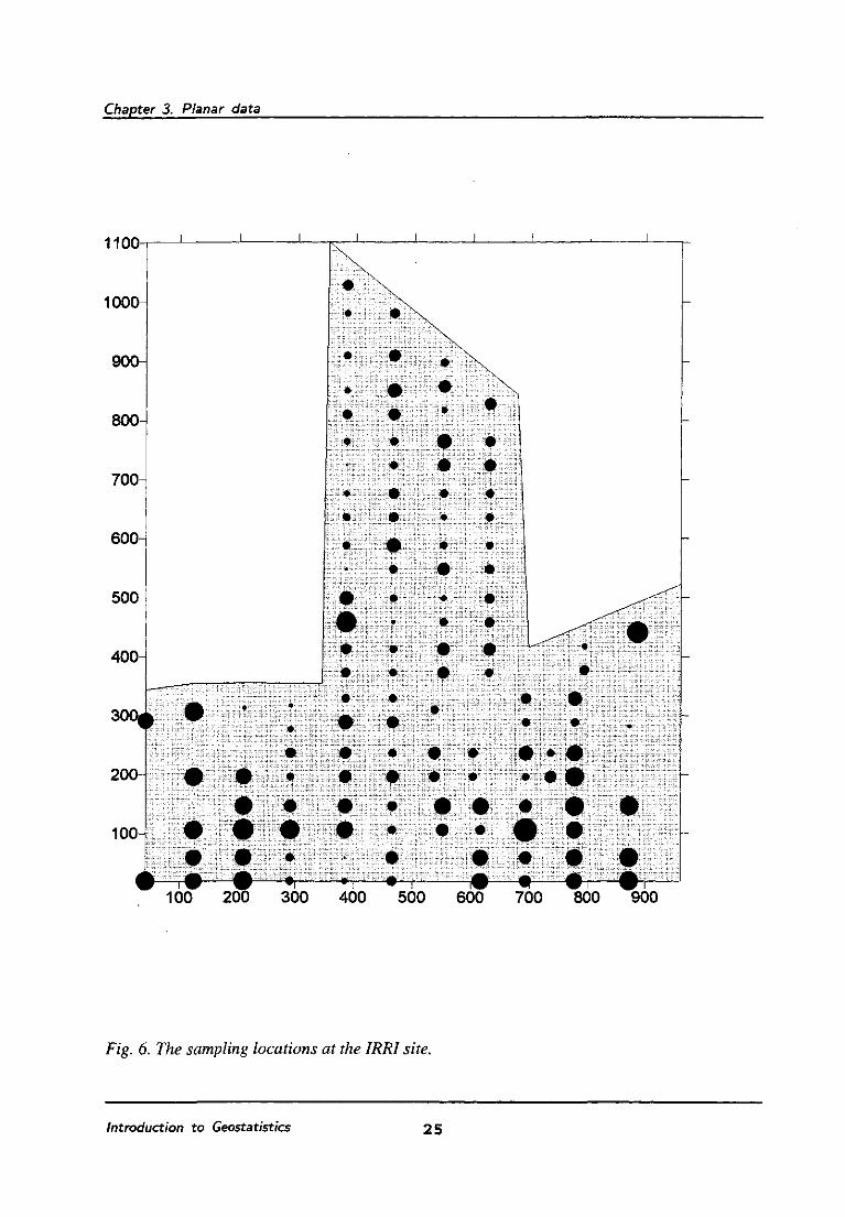
Exercise A 50 ha study area at the experimental farm of the International Rice Research Institute (IRRI) in Los Bahos, Philippines, was sampled in 1991. The area is embedded between two creeks that have deposited alluvial material originating from Pleistocene and more recent volcanic activity. The alluvial portion of the profile becomes thicker from the elevated north-south central part of the area towards the creeks. Depth to an unweathered volcanic tuff layer in the central part varies strongly over small distances and ranges from close to the surface to a depth beyond the reach of an auger (2.2 m). The study area is gently sloping and consists of moderately well drained clay soils. The soil survey was made at a scale of 1: 6000 on a regular 40 m x 80 m grid. A total of 144 auger observations were made to a maximum depth of 2.2 m or to the upper surface of the unweathered volcanic tuff layer.

Select a variable of interest, e.g. thickness of the puddled layer (col. 3), depth to the mottled layer (col. 5) or depth to the tuff layer (col. 8). Take the number of lags equal to 20, and the lag length to 40 m. Keep the stratification variable at 0 (we will consider stratification in the next chapter). Consider 2 directions: 0°, and 90° and take a direction tolerance equal to half the direction interval, i.e. 45°. Answer the following questions: - Is there strong evidence for the existence of anisotropy?



1100

1000

900-

800

700-

600

500

400

3 0 0O

200

100

100 200 300 400 500 600 700 800 900

Fig. 6. The sampling locations at the IRRI site.



- what could be the cause for the anisotropy?

Repeat the calculations with the robust estimator f or the semi-variogram. - what happens if the robust instead of the 'classical' semivariogram estimator is applied? Repeat the calculations with other direction tolerances (5° or 30°). - what happens if the direction tolerance changes?

For several applications indicator data (data taking the value 0 or 1 only) are suitable.

Such data are usually obtained as follows: consider a continuous spatial variable that takes its

values in a 2-dimensional space. And suppose there are some fixed threshold values, for example

the target level or the intervention level. From the original variable new variables are constructed,

one for each threshold value. This variable takes the value 1 if the original variable exceeds the

threshold value and 0 otherwise. For example, from a Cadmium variable Cd(x) the indicator

variables li(x), U(x) may be obtained, which take the value 1 if the variable Cd(x) exceeds the

target level and the intervention level, respectively. Evidently, Irfx) can only take the value 1

([Cd] > intervention level) if Jj(x) has the value 1. For such variables also semivariograms may

be constructed, called indicator variograms.

Indicator variables play an important role when probabilities of exceeding threshold

values have to be determined. In fact, the expectation of an indicator variable equals the

probability that this variable exceeds the threshold value: E[lj{x)] - 0-P(lj(x) = 0) + 1 -P(lj{x)

= 1) = P(lrfx) = 1).

It has been remarked in the introduction of this chapter that random fields may be

generated by means of the turning bands methods. This is just one of the existing procedures.

Simulation of random fields may be helpful for several purposes, such as checking what variation

occurs as output from a model when it is subject to random fluctuations, to evaluate the effect

of sampling schemes, etc. Many software packages, like ISATIS and GSLIB contain simulation

techniques. Simulated fields with the same set of parameters may differ considerably. Even if

these fields are conditioned on observations, differences in unvisited parts of the area may be

quite high. We will not pay further attention to simulated fields. The interested reader is referred

to the books of Journel and Huijbregts (somewhat outdated), Deutsch and Journel and Cressie

(rather concise).



Chapter 4 Stratification

In geographical information systems, digitized soil maps may be available. This

information, if possible, should be used to improve modelling of the semi-variogram. In the first

place, different units may show different mean values: on a 1:250,000 soil map the unit M13

(heavy clay) will be different from unit Z27 (sand) as concerns the regionalized variable clay

content. In the second place, different soil units may show a different internal spatial variability.

Some units are homogeneous with respect to a regionalized variable, i.e. the variable shows

relatively little variation between different locations, whereas other units are heterogeneous,

showing large variability between different locations. We therefore distinguish deterministic

flucjuations (given by the map delineations) and random fluctuations (given by internal

variability).

Using a combination of prior information and spatial statistics allows us to take evident

non-stationarity into account. Differences in soil properties may be much larger in one part of an

area as compared to another part of the area and soil pollution may be large in some parts of

factory premises and minor in other parts. Stratification has been recognized by soil surveyors,

geologists and hydrologists for a long time. Traditionally, such variations is taken into account

by creating a choropleth map like a soil map. Soil delineations take the major, evident differences

into account, homogeneity may be assumed within the delineated areas. The delineated areas will

be termed strata. ycj\ i^mrw>*<'-<;£•'}.

The value of the standard deviation masks a possibly different functional relation of the

spatial variability between different strata. Therefore, different semivariograms for a regionalized

variable may apply to different strata: often regionalized variables exhibit a different spatial

structure within each stratum. It is usually illusory, as is suggested by choropleth maps, to

suppose that strata distinguished on the basis of sedimentation history, soil genesis, pollution

history or whatsoever are homogeneous with respect to soil physical properties or soil

contamination.

Formally, stratification can be described as a partitioning of the study^area. After



stratification the area is divided into, say/?, different strata Ay, A2, ..., Ap, none of which is empty,

having an empty intersection and together cover the total area:

A/ uA2 U... uAp =A;

Ai nAj = 0 for i #;';

A, ̂ 0 for all i.

Within each stratum A, (i=l,...,p) a (soil) property is described by a regionalized variable

Yj(x), i = l,...,k, all depending on the location vector x.

Stratified semivariograms are constructed for each of the delineated strata. Each stratum,

therefore, should contain sufficient data to allow estimation. Stratification of an area can only be

performed when the level of stratification is high. Detailed stratification only permits the

construction of semivariograms in some of the strata. But nonetheless it requires at least 50-60

observations in each stratum. In several studies stratification has been proven to be successful:

for interpolation purposes different semivariograms in different parts of an area reveal often

interesting information. It essentially uses information that is available, for example in the form

of a soil map.

Exercise The 404 ha Mander area in the eastern part of the Netherlands has been used for groundwater extraction since 1955. Due to water shortage caused by this water extraction, water tables in the area were lowered and in dry periods crop yields of some of the local farmers decreased. By means of a study carried out by the Winand Staring Centre, individual losses of farmers were calculated. A total of 499 observations on basic soil properties, like rooting depth, organic matter content, clay percentage and former and present mean highest and mean lowest water table were obtained by means of a 1:10,000 soil survey, carried out in 1985. In the study area three different soil types were found that are classified as Humaquepts, Haplaquods and Plaggepts. All soils developed in cover sands and are relatively wet, as indicated by soil mottles, except for the Plaggepts. Current water tables were measured. Levels that occurred before the period of water extraction were estimated by the soil surveyors using soil mottling criteria.

The simulation model LAMOS was used to calculate moisture deficits caused by lowering of groundwater tables in the Mander area. Calculations of this model are based on observations of soil variables on meteorological data



and on data on groundwater extraction. Two different moisture deficits for grassland were calculated under the

present hydrological situation, the moisture deficit for 1976 (MD76), an extremely dry year, and the yearly average moisture deficits for the period 1956 through 1985 (MD30).

The LAMOS model makes a distinction between topsoil and subsoil. The latter can be composed of different layers. Moisture retention curves are needed for both top- and subsoil. Hydraulic conductivity curves are needed for the subsoil only. Measurements were made in the context of the original study. Hydraulic conductivity and moisture retention curves for all 499 points being considered in this study are based on measured data in well defined soil layers. Thirteen moisture retention curves were distinguished for the topsoil and fifteen curves for layers of the subsoil. In addition, fifteen hydraulic conductivity curves were distinguished f or layers of the subsoil. Soil layers were defined in terms of soil texture (i.e. loam content) and organic matter content. Calculation of moisture retention curves was based on regression analysis using organic matter and loam content as explanatory variables.

Use the Mander data file MANDER.DAT. Take a variable of interest, e.g. MD76 or MD30. Use the program SPATANAL. Take soil types (col. 6) as the stratification variable. Use 20 lags with a lag length of 0.05 km. Do not analyze different directions because of lack of sufficient data for every combination of direction and stratum.

Notice the differences in mean value and in standard deviation. Notice the

differences in estimated semivariogram parameters (model, nugget, sill and

range). Explain the observed differences.

The availability of sufficient data for each different stratum is rather restrictive. As an

alternative a so-called within-strata semivariogram can be applied. This semivariogram is

estimated by using only pairs of points for which both points fall within the same stratum. Pairs

of points of which one point falls in one stratum and the other point in another stratum are

discarded. Such semivariograms may give information whether stratification is useful (gives a

large reduction in the original semivariogram) as compared to lack of stratification.

Exercise Use the same data set, and estimate the within strata semivariogram for the same variable as before with the program SPATIN. Use similar values for number of lags and for length of lag. Observe the reduction in spatial variability as expressed by sill, range and nugget.

To create strata in an unstratified area, use can be made of different procedures. The most



obvious way is a soil survey or a land survey, yielding homogeneous units on the basis of a

classification system. However, also numerical and statistical techniques may be applied. These

procedures are in particular fruitful when observations on several variables are included and for

which no classification system exists. For example, soil contamination data and data derived

from Digital Elevation Models can be classified in a sensible way. A modern example of a

classification technique is fuzzy clustering.


Chapter 5: Spatial prediction and kriging

Chapter 5. Spatial prediction and kriging

One of the central activities in studies on spatial variability is to arrive from point

observations towards area (or line) covering statements. The most simple example concerns

observations collected along a transect. Based upon a limited number of observations one wants

to predict the most likely value in an unvisited location. Also, one wants to obtain a measure of

the quality of this prediction, such as the variance. Sometimes, also extrapolation comes into

view. This is always hazardous, but if necessary also a measure of the uncertainty has to be

obtained.

There is a crucial difference between estimating the expectation in an unobserved point

and predicting the most likely value in the same point. If one simply estimates the mean value

m, assuming uncorrelated disturbances, all with the same variance, the best prediction and the

estimate of its expectation for a new point with regressor values contained in the vector x0 take

the same value (i. However, if the expectation is estimated, the uncertainty is only to be attributed

to uncertainty in determining m. When predicting, additional uncertainty has to be dealt with,

because an individual observation has to be predicted. Apart from numerical differences

prediction of a random variable and estimation of its expectation are fundamentally different.

From now on we deal mainly with prediction, that is in fact estimation of a stochastic effect.

Consider the problem of guessing a variable Y(x) in an unvisited location x0. The first

approach would be to estimate the average value |i and assigning this value to x = x0, being a

prediction for the value of Y(x) in x = x0. One can prove that it is even the best linear unbiased

prediction. The variance of the estimation error equals cf/n, where a2 equals the variance of Y:

Using standard computer routines an estimate for s is obtained from:

G' = ( n A j

n-\ ^yf-n-y1 = T^ivi-yJ

n-\~7

To summarize: using standard statistical software calculation of the estimation of the expectation

and its uncertainty is easily being done.



The variance of the prediction error, however, differs from the variance of the estimation

error. It is equal to (l+l/n)cr. In fact it is equal to the sum of the variance of the estimation error

and the variance a" of Y. This value will only incidentally be obtainable from computer routines.

Exercise Consider the following 7 observations on bulk density:

1

4.07

2

5.12

4

5.29

5

6.16

6

7.12

8

11.73

10

15.58

Location

Bulk density

Put the data in a spreadsheet. Determine the mean value ß (use the function ©average) and the standard deviation (use @var and @stdevj of bulk density. Predict the bulk density as well as the variance of the prediction error in the points with locations 0, 3, 7, 9 and 25. Determine also the variance of the prediction error and the variance of the estimation error.

Predicting in the presence of spatial dependence slightly differs from the procedures

outlined above. Basic fact is, again, that we know that observations close to each other are more

likely to be similar than observations located at a greater distance from each other. This implies

already intuitively that it is highly unlikely that all the predictions are equal to the mean value:

deviations from the mean are likely to occur, especially in the neighborhood of largely deviating

observations. If an observation is above the regression line, then observations in its neighborhood

will be above this line as well.

Carrying out predictions is associated with a prediction error. We will focus attention on

predictors, linear in the observations (that is: each observation is assigned a weight) that are

without bias (that is: the predictor may yield too high a value or too low a value, but on the

average it is just right).

So let the optimal predictor be denoted with Y(x0). It is linear in the observations,

therefore

Introduction to Ceostatistics 3 2


with as yet unknown weight X,. Aim is to predict the value of Y(x0) in the unvisited location x0.

For the prediction error e = Y(x0) - Y(xn) it is assumed that its expectation is zero (E[e] = 0) and

that its variance is minimal among all linear unbiased predictors: Var(T(x0) - Y(x0)) is minimal.

The variance of the prediction error is of importance and is to be calculated below.

In the case of spatial dependence among observations predicting requires knowledge of

the semivariogram. Suppose therefore that there are n observations, that a semivariogram has

been determined and that one of the models of the Appendix has been fitted and that its

parameters were estimated. The semivariogram values can be determined for all distances

between

a) all pairs of points consisting of observation points (which are Vm{n-1) in number);

b) all pairs of points consisting of an observation point and the prediction location (which are n

in number).

All the semivariogram values obtained with a) are summarized in the, symmetric, nxn

matrix G. The elements of G, gy, are then filled with the values obtained with a): gy - y(\xi-xß);

gu contains the semivariogram for the distance between xj and xj, a pair of points with distance

equal to zero, and hence gu - 0; gn contains the semivariogram value for the distance between

xj and X2 and is equal to g2i. Also, gi3 contains the semi-variogram between xj and xs, etc. Notice

that gjj = gji and that all the diagonal elements gu of G are equal to 0.

All the semivariogram values obtained with b) are contained in the vector g0. The first

element of go contains the semivariogram value for the distance between xj and the prediction

location xo, the second element of go contains the semivariogram value for the distance between

X2 and xo, etc.

The unbiased predictor with lowest variance of the prediction error, linear in the

observations is given by:



Y(x0) = ^lY(xi) = fi+g0:G-'(y-fi-O

where 7„ is the vector of n elements, all equal to 1. An estimate for the value of fi (different from

the average value!) is found by means of the generalized least squares estimator

fi = {jn<j'In)'InG 'y



Calculation of the predictor t is carried out with computer routines. The main task is to invert the

n xn matrix G.

Example. Along a straight line two observations of a variable, with values equal to 21 and 23, were situated at locations zi and Z2 with coordinates 1 and 3, respectively (fig. 7). The semi-variogram y(r) is were assumed to be known, and to obey an exponential model with nugget effect: y(r) = B-(l-Ô(h))+A(l-exp(-h/b)), where b\r) = 1 if' r - 0 and S(r) = 0ifr^0. The values ofB, A and b are equal to 1, 3 and 0.5, respectively. The value of ßb equals the average of the two observations. This yields the following intermediate results:

Y = ''27 ^

23

( i \

; h = v7;

:G = 0 3.945

3.945 0 ; V = 1.976; ß = 22.000

Predictions were carried out for all points with coordinates between 0 and 4 (fig. 7), standard deviations of prediction error are given in fig. 2. Numerical attention is focused on the locations Pi, P2 and Pi with coordinate 2, 2.5 and 3.5, respectively. Point Pj is of interest as it is the center of between the observations, point P2 is an interior point for which typically predictions are needed, e.g. if a map is to be constructed, and with point P3 extrapolation can be illustrated. The vector go is different for each of the three predition locations:

Pi-gc 3.594

3.594 P2--g0 = 2.896A

3.851 • P3-'gn = 2.896

3.980

After matrix multiplication and addition (check!) we have the following predictions:

Y(P1) = 22.0; f(P2) = 22.24; Y(p3) = 22.28;

The prediction in the center point is equal to the mean of the two observations. The predictions in the other points somewhat deviate.



23

22

c o o

TD CD

21

20

location 4

F/g. 7. Position of observation locations, predictions (straight line) and variance and standard deviation of the prediction error (dashed lines). Notice that the prediction passes (discontinuously) through the observations, and that the uncertainty equals 0 in these points.



r

The prediction equation consists of two terms: apart from the overall (generalized)

mean//, the term go'G''(y-fi ln) is included. This second term expresses the influence of the

residuals (y- fi ln) of the observations y with respect to the mean value fi ln on the predictor. The

residual are transformed with go'G'1, modeling the spatial variation, by means of the

semivariogram, among the observation points and between the observation points and the

prediction location.

Predicting an observation in the presence of spatially dependent observations is termed ( •

Kriging, after the first practitioner of these procedures, the south-African mining engineer Daan

Krige. His field of study were the Witwatersrand gold mines. The theory has been developed

further mainly by the french École de Mines in Fontainebleau, where the work of Matheron and

his co-workers have given these procedures general validity, theoretical background and

acceptance. Currently, geostatistics and kriging are applied in many environmental and mining

studies.

Exercise Use the same data as in the previous exercise. Assume that the spatial dependence function (the semivariogram) as a function of the distance h between observations is given by a linear model without sill "rfh) - 2+4-h. Write down the matrix G and the vector go when a prediction has to be carried out in the point xo with coordinate equal to 3. What is Y? Compare an estimate for fi with the calculated mean value.

It has already been argued that every prediction is associated with a prediction error. The

prediction error itself can never be determined, but its variance has been determined already in

case of spatially uncorrelated data. In situations of spatial dependence, an equation to obtain the

prediction error variance is given by

Var(Y(x0)-Y(x0))=gff'G-'g0-xa2-V

where the numbers xa and V are defined as



Xa= l-g(fG~' In

v = 1

(In-G'h)

All matrices and vectors can be filled on the basis of the data, the observation locations

and the estimated semivariogram.

Example For the data of the previous example, the values for go, G, I2 and V are the same. The values for xa are equal to:

p, : Xa = -0.822; p2 : Xa = -0.710; p3 : Xa = -0.742;

We then obtain the following terms which together constitute the prediction error variance:

Pi p2

Ps

go'G~'go

6.548 5.654 5.844

Xa'Vxa

1.333 0.995 1.089

Var(t-yo)

5.215 4.659 4.755

We remark that the prediction error variance depends only indirectly upon the observations: the

vector y is not included in the equation. However, the estimated semivariogram is estimated on

the basis of the observations. The configuration of the n observation points and the one prediction

location influences the prediction error variance as well.

One remark on the use of neighborhoods: the predictor is linear in the observations. The

weights (perhaps the term 'coefficient' should be preferred, since negative weights are

encountered as well) become smaller with increasing distance from the prediction location.

Practice has evidenced that it suffices for most practical studies to use neighborhoods containing

8-12 points to make a prediction.

n

Exercise The predictor Y(x0) is a linear predictor, i.e. Y(x0) = £^À,iY(xj)=A.'Y, where



Y is the vector of observations and X is the vector of weights. Determine an expression for X.

In the next exercise we will determine predictions and the prediction error variances for

Cadmium data of the Kempen. Different neighborhood sizes will be used.

Exercise Use one of the variables collected in the file CDTRAN.DAT (cf. exercise 1). Determine first (if necessary) the semi-variogram. Predict values in the locations 10.0, 10.1, 10.2, 10.3, 10.4, 10.5, 10.6, 10.7, 10.8, 10.9 and 11.0 and register the prediction error variances. Predict also in the locations -1, -2, -3, -5 and -10. Use neighborhoods of size 4, 8 and 12 points. Summarize the influence of its size and of the location of the prediction point on prediction and variance of the prediction error.


Chapter 6: Spatial interpolation

Chapter 6. Spatial interpolation

In geographical information systems, one may need a map of a spatial property. For

example, proper reference with other data, or combination of different map overlays should be

aimed at. If a map has to be constructed of a spatial property for which the observations are

collected in a 2-dimensional space (for example the available water in a river terrace, the cyanide

content in a polluted parcel or the clay content in a polder area) the following procedure may be

used:

a) Determine the semivariogram;

b) Fit a model to the semivariogram;

c) Predict values at the nodes of a fine-meshed grid;

d) Present the results in a two- or a three-dimensional perspective by linking individual

predictions with line elements.

Predicting in two dimensions is therefore similar to predicting along a transect. In

addition to the map itself, it may be desirable (and sometimes even necessary) to display the

prediction error variance (or its square root), which is obtained at the same nodes of the fine-

meshed grid as the predictions themselves. This map displays the spatial uncertainty of the map.

It is important to distinguish interpolation from extrapolation, i.e. predicting outside the

observation area. It is always risky to extrapolate. The prediction error variance rapidly increases

beyond the observation area. When an extrapolation is needed, the prediction error variance

should always be included, e.g. in order to give the uncertainty of the prediction.

Each map may displayed in several possible ways. Modern computer facilities allow to

make a distinction into:

1. In the form of a contour map: equal values are connected with each other and the connecting

lines (isolines) are displayed (computer packages Surfer and Arclnfo)



1000

600

E 600

400 -

200

200 " T — i — i — i — r

400 600

1000

BOO

- 600

400 600 Y-coordlnate [m]

BOO

3D-perspectiv«

X Mfi . „ l<"]

Ll»] Fig. 8. The variable 'Depth to the tuff layer' at the IRRI site displayed in a 2- and a 3-dimensional perspective, respectively.



2. In a three-dimensional fashion: the distribution of the values in a region is displayed in the

form of a mountainous landscape: high clay percentages are the mountains, low clay

percentages are the valleys (computer packages Surfer and Arclnfo).

3. In the form of grey-shading: high values are black, low values are white (or vice versa). Such

maps usually are very easy to display the essentials of a map (computer packages GSLL3

and IDRISI).

4. In the form of a colour map: areas with (more or less) equal values are delineated and are

assigned a colour to. This type of displaying has an additional uncertainty, since

delineating areas may be done quite arbitrarily (computer packages IDRISI and Arclnfo).

An overview of computer software to arrive at such maps is given in the appendix.

Whatever display is preferred, the maps must be readable, have a proper legend, all axes

must be included and the units of measurement should be given. When maps have to included

in scientific publications, some reference in the form of topographical features should be included

as well.

Exercise Determine a (predictive) map of one of the variables in the IRRI.DAT file. Proceed along the following steps: 1. Use SPATANAL to determine the semi-variogram. Use 15 lags with a lag length of 40 m. Do not analyse anisotropy, do no apply stratification. 2. Use WLSFIT to estimate the proper semi-variogram model. Note the values for sill, range and nugget effect. 3. Use MAPIT to interpolate from points to grid nodes. For MAPIT the semi-variogram information must be given, as well as the minimum x (take 0), the maximum x (take J000), the minimum y (take 0) and the maximum y (take 1100). Also the grid mesh must be specified: a low number of grid nodes (say 25) gives a rough impression, but is fast, a large number of grid nodes (say 100) gives a fine impression, but the calculation time is 16 times as large as for 25 nodes! The prediction and the standard deviation of the predistion error files are saved as MAPxxxxx.GRD and ERRxxxxx.GRD, where for xxxxx a short acronym, based on the name of the variable is given. These files can be imported into SURFER 4. Use the SURFER program to display the maps: the map with the prediction in a 3D perspective, the map with the standard deviations of the prediction error as a contour map. Post the observation points in the 'error'-map.

There are other ways to arrive from a collection of point observations towards areal



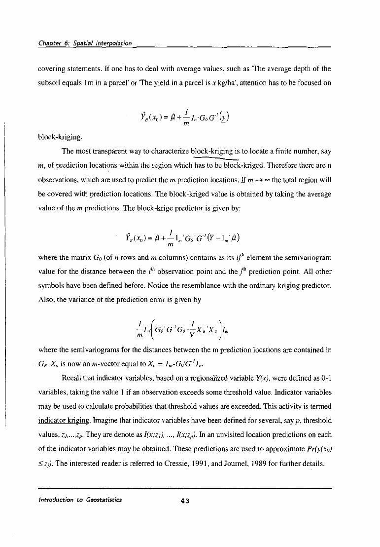
covering statements. If one has to deal with average values, such as 'The average depth of the

subsoil equals lm in a parcel' or 'The yield in a parcel is x kg/ha', attention has to be focused on

YB(x0) = fi + — l,n>GoG'{y) m

block-kriging.

The most transparent way to characterize block-kriging is to locate a finite number, say

m, of prediction locations within the region which has to be block-kriged. Therefore there are n

observations, which are used to predict the m prediction locations. If m —» °° the total region will

be covered with prediction locations. The block-kriged value is obtained by taking the average

value of the m predictions. The block-krige predictor is given by:

YB(x0) = fi + -\m'Go'G'(Y-\„;ß) m

where the matrix Go (of n rows and m columns) contains as its if1 element the semivariogram

value for the distance between the z'th observation point and the fh prediction point. All other

symbols have been defined before. Notice the resemblance with the ordinary kriging predictor.

Also, the variance of the prediction error is given by

1 -In m

. -i } . ' Go G Go 'rrXu Xü In

where the semivariograms for the distances between the m prediction locations are contained in

Gp. X« is now an m-vector equal to X„ = lm-Go'G~lln.

Recall that indicator variables, based on a regionalized variable Y(x), were defined as 0-1

variables, taking the value 1 if an observation exceeds some threshold value. Indicator variables

may be used to calculate probabilities that threshold values are exceeded. This activity is termed

indicator kriging. Imagine that indicator variables have been defined for several, say p, threshold

values, zi,...,zp. They are denote as I(x;zi), ••-, I(x;zp). In an unvisited location predictions on each

of the indicator variables may be obtained. These predictions are used to approximate Pr(y(x0)

<Zj). The interested reader is referred to Cressie, 1991, and Journel, 1989 for further details.



An approximation of the probabilities that a variable exceeds some threshold value may

as well be obtained by means of disjunctive kriging. Essentially, the observed distribution of the

variables is transformed into a normal distribution by means of so-called Hermite polynomials.

These are used to predict the distribution in a prediction location, followed by back-

transformation. Refer to Cressie, 1991 for more details and appropriate references.

Still other techniques exist and have their merits for particular problems:

1. Splines

Splines are used successfully to interpolate small data sets (for which no semi-variogram

can be determined). They are applied in meteorological studies. A Laplacian

smoothing spline of degree 1 for obtaining a value at location s0 = (xo.yo) in a two-

dimensional space is defined as:

n

Zspline ( Su) = « 0 + Ofl X0 + (Xl y 0 + X ß> e ( S 0 ~ S i ) k=l

where the function e(h) is defined as e(h) = \h\2 log(\h\2)/(16p) and the n observations are

available at the locations s, = (xi,yj (i = l,...,n). Values for the unknown coefficient

vector a = (ait i = 0, 1, 2) and ß= (ßj, j = J,...,n), are obtained by means of solving the

linear equations

Xa + (E + npl)ß =Y

X'ß =0.

The vector Y contains the n observations, the matrix X is the matrix of size n x 3 with as

its ith row the elements 1, x, and y„ E a matrix of size n x n contains as its //th element

evaluation of e(h), evaluated for the distance between s, and Sj, the matrix I is the n x n

unity matrix and p is a positive real number. The value of p that provides the best

estimator for the value in s0 is determined by means of cross-validation.

2. Inverse distance

For inverse distance interpolation, weight X\ are assigned to observations, which are

proportional to the inverse distance between a prediction point and an observation point.

Sometimes the distances are squared. Inverse distance routines are applied under the



same conditions as splines: relatively few observations are available, and a 'quick and

dirty' map is preferred to an optimal map: the prediction error variance is larger for

inverse distance techniques than for kriging. Also, no spatial variability is taken into

account: every variable is interpolated with the same procedure, despite possibly different

spatial heterogeneity.

3. TIN

TIN procedures, available in GIS, combine observations by lines. For some data, such as

elevation data, these techniques have been applied successfully.

4. Trend surfaces

Trend surfaces give a global, in stead of a local pattern of spatial interpolation. They

might give a general picture of the variable in the region.


Chapter 7: Spatial sampling

Chapter 7. Spatial sampling

An important issue in geostatistics concerns the design of sampling plans. The problem

can be briefly summarized as how many measurements are needed and where should they be

located in an optimal way. The main problem then is: which design is 'optimal', and in what

sense? We will focus in this chapter on one particular optimality criterion: to design a sampling

Q scheme for optimal mapping, that is mapping with a given, pre-scribed. Precision.

We will assume that the semivariogramisknown, and that we want to determine the

sampling design in order to create a map of a predetermined precision. This situation is more

common than it appears at the first sight. For example, the semivariogram may be available from

a previous survey, or from a pilot study. Also, multi-staged sampling procedures could be used,

and evaluation between different stages might involve the semi-variogram.

We will use the kriging equations for the predictor and the prediction error variance to

obtain predictions with a certain prescribed precision. A scheme is optimal if no other scheme

with the same number of observations yields a map for which the maximum occurring standard

deviation of the prediction error is lower. We recall that the maximum occurring kriging standard

deviation occurs at those points which are furthest away from the prediction point. If we located

points in a random way over the area, clusters of points tend to form as well as sub-areas which

are sparsely sampled. Such a scheme is therefore sub-optimal to a regular scheme, for which

every sub-area is equally densely sampled. Also, collecting data along transects for which the

separation distance is different from the sampling distance is sub-optimal as compared to grid

sampling.

In principle, three different designs can be considered: triangular grids, square grids and

hexagonal grids. Deciding upon an optimal scheme runs as follows: whenever a sampling type

is chosen, e.g. the type of a grid, one could vary the distances between the observations and recalculate the prediction error variance. Since the prediction error variance depends solely on the

data configuration (which we may vary) and the semi-variogram (which is given), but not on the

data, actual observations are not necessary. The maximum uncertainty can be quantified for



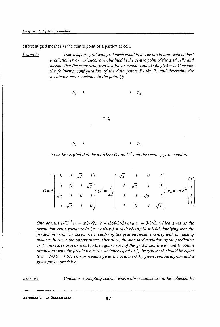
different grid meshes as the centre point of a particular cell.

Example Take a square grid with grid mesh equal to d. The predictions with highest prediction error variances are obtained in the centre point of the grid cells and assume that the semivariogram is a linear model without sill, g(h) = h. Consider the following configuration of the data points Pi t/m P4 and determine the prediction error variance in the point Q:

P4 P3

Q

P2

It can be verified that the matrices G and G and the vector go are equal to:

G = d

( 0 i 45 r

1 0 1 42

41 1 0 1

, 1 42 1 o\

G ~2d

(-4~2

1

0

1

1

-42~

1

0

0

1

-4~2

1

1^

0

1

-4-2)

:'8o = idJ2

fl) 1

1

in

One obtains go'G go = d(2-v2), V = d/(4-2\2) and xa = 3-2v2, which gives as the prediction error variance in Q: var(t-yo) = d(l 7^/2-16)/J4 ~ 0.6d, implying that the prediction error variances in the centre of the grid increases linearly with increasing distance between the observations. Therefore, the standard deviation of the prediction error increases proportional to the square root of the grid mesh. If we want to obtain predictions with the prediction error variance equal to 1, the grid mesh should be equal to d - 1/0.6 - 1.67. This procedure gives the grid mesh by given semivariogram and a given preset precision.

Exercise Consider a sampling scheme where observations are to be collected by



means of an equilateral triangular, a square or a hexagonal grid. Use the same semivariogram as in the example above. Which distance is necessary to achieve a prediction error variance equal to 1 ?

Exercise Assume that for the IRRI.DAT file the question is relevant whether to stop sampling, or to continue. This question is subject to the precision of the final map for the depth to the tuff layer. Make a chart which gives the accuracy as a function of the grid mesh. Use first the SPATANAL and the WLSFIT program

• to estimate the semi-variogram. Use the OPTIM program to compare different grid designs and meshes and different degrees of precision.

A choice for any particular sampling scheme strongly depends upon the optimality

criterion. There are probably no schemes which are optimal in every sense: optimal estimation

of the semi-variogram, or optimal estimation of the average value within a particular delineated

unit requires different sampling.

1. When predictions have to be carried out the area should be covered with observations as

regularly as possible. Avoid highly sampled subareas as well as sparsely sampled

subareas. This leads to a (square, triangular or hexagonal) grid as outlined above.

2. To determine the semivariogram observations close to each other as well as observations

separated by a larger distance should be collected. Closely neighboring observations

contribute to estimating the nugget effect, observations at a larger distance contribute to

estimating the sill value. A grid with some additional short distance replicates should be

used, because it is usually still important to have the area reasonably covered with

observations (in order to minimize the risk of missing important information).

3. A scheme should be operationally feasible. In many practical studies it has been shown

that the use of transects is very adequate to collect spatial observations. A reduction in

the precision of the predictions may (far) be compensated by an increase in operationality.

The procedure applies especially when one has to deal with variables that are to a certain

degree stationary. When 'hot spots' are to be expected (say on the basis of prior information) a

sampling scheme may have a higher density around these hot spots as compared to regions where

these hot spots are not to be expected.

Of course there are other boundary conditions to be included when designing a spatial



sampling scheme. One may think of practical limitations given by the analysis capacity in the

laboratories, the number of available field workers and hand computers, but also of the natural

side conditions like accessibility, the appearance of anisotropy, etc. In general the design of a

spatial sampling scheme needs an important investment of skilled intellectual input.

In cases that nothing is known: the reader is referred to Webster and Oliver, 1990. It

suffices to take 50-60 observations, more or less regularly distributed in the sampling area with

some observations close to each other and some separated at a larger distance. Sampling

following a grid pattern may be preferable, also from an operational point of view.

The main drawback is that there is regularly far more (prior) information available.


Appendices

Suggestions for further reading.

Applied books:

Davis, J.C., 1986. Statistics and data analysis in geology, 2nd edition. Wiley, New York, 646p.

Deutsch, C.V., and A.G. Journel. 1998. GSLIB. Geostatistical Software Library and User's

Guide. Oxford, Oxford University Press.

Isaaks, E.H. and R.M. Srivastava. 1989. An introduction to applied geostatistics. Oxford

University press, Oxford.

Webster, R., and M.A. Oliver. 1990. Statistical methods in soil and land resource survey. Oxford

University Press, Oxford, 316p.

Theoretical books:

Christakog, G. 1992. Random field models in earth sciences. Academic Press, New York.

Cressie, N.A.C. 1992. Statistics for spatial data. Wiley, New York, 900 pp.

Journel, A.G. and C.J. Huijbregts. 1978. Mining geostatistics. Academic Press, London, 600p.

Software:

GEOEAS: a userfriendly, interactive package that is easy to use and covers much of the

procedures used in this course. Operating system: MSDOS.

MAPIT + SURFER: a combination of two packages that focuses entirely on the topics in this

course. It is less well interfaced, but the power and the applicability are more in line with

the requirements from soil scientific studies. Operating system: MSDOS.

GSLIB: nice public domain software, available as Fortran source. Contains simulation routines.

Operating system: any system that supports a fortran compiler.

ISATIS: expensive, but completely state-of-the-art software. Semivariogram analysis,


Appendices

interpolation and simulation. Runs currently on UNIX.

ARCINFO: Geographical Information System, that has recently been extended with a Kriging

module. Runs on VMS (VAX).

EDRISI: A cheap raster based Geographical Information System, developed at Clark University.

Runs on MSDOS.


Appendices

Semivariogram models

A distinction can be made between transitive models (which apply to fields which have

a finite variance) and infinite models. Commonly used transitive models are:

0 forh = 0 Nugget effect: yN(h) =

Co forh±0

A*± forhe(0,b] Linear model with sill:" YL(h) =

A for h>b

A*(JL(h.\ ±( k \s\ for h e (où]

Spherical model: 7SW= ^ U ; ' J

A for h>b

Exponential model: YE(h)= A*[l -e*) forh>0

Gaussian model: yG(h)= A*\l - e'i~h)forh>0

Hole effect (or wave) model: yw (h) = A * (l - \ * sin( •*- )) forh>0

yc(h) =A*{7-f*cos-Vi)-fi7^ for h e (Oh]

Circular model: ' " ~ " V ~K Wi>w**r~V = 0 jurh>b

Bessel model: yB(h)=A*b*h*K,(b*h)forh>0

h2

Rational Quadratic Model: yp(h) = A*

'* l+h2/b

Properties

/ Any sum of semi-variogram models can be made, yielding a so-called nested semivariogram.

H By definition, yx(0) = 0 for each of the types X=N, L, S, E, G, W, P, C, B and R. In all

the equations Co, A and b, or k and m, are positive parameters, and are to be determined

from the original data.

Hi The linear model with a sill ydN is only permissible for data along a transect, but not for


Appendices

planar data or for data in 3 dimensions.

iv The function K](h) is the modified Bessel function of second kind of order one.

v The exponential model yE(h) never reaches the sill value (nor does the Gaussian model,

the Bessel model, the Hole effect model and the Bessel model). The parameter b is

therefore associated with the range, but not similar to the range. It is common practice for

yg(h) to define the range to be equal to 3b, which is the distance where the y^h) reaches

95% of the sill value. Similar values apply for the other models.

vi The Gaussian model is characterized by its horizontal behaviour at the origin. This model

is encountered, a.o., when there is uncertainty with respect to the precise location of the

observations.

vii The hole effect (wave) model is regularly encountered in practice. It points to periodicities

of the variable, caused by human influences, deposition, etc. Interpretation of such

periodicities is often important.

viii The Bessel model and the circular model are not so often encountered in practice.

The most common infinite model is the power model:

Power model: yp(h) = k- h"' with 0<m<2; for h>0 .


Appendices

Glossary

(Based upon R.A.Olea - Geostatistical glossary and multilingual dictionary, Oxford University

Press, 1991).

Geostatistical terms:

Anisotropy - the quality or state of not possessing isotropy.

Block kriging - estimation by kriging of average values defined over a support larger than the

support for the observations; for example yields should be estimated by block kriging.

Dependence - the set of relations linking the values of a regionalized variable at different

locations in space. Spatial dependence usually arises from a common genesis and is used

with advantage in predicting an unsampled value from neighboring observations.

Expectation - let y be a random variable having a probability function f(y) and let u(y) be a

E[u(y)] =\ u(y)f(y)dy

function of y. If y is a continuous variable, the expected value of u(y) is defined as

E[u(y)] = ^u(y)f(y)dy y

If y is a discrete variable, the expected value is defined by

The expected value exists if and only if E[\u(y)\] < oo.

Independence - lack of dependence.

Intrinsic - A random field Y(x) is said to follow the intrinsic hypothesis (or is called weak

stationary) if simple differences (Y(x) - Y(x+h)) are stationary: there expectation exists,

and their variance is independent on the location x and is solely depending on the distance


Appendices

h between locations.

Isotropy - the characteristic of a semivariogram (or covariance function) to depend only on the

modulus \h\ of the separation vector h, and not on its direction.

Kriging - A collection of generalized linear regression techniques for minimizing the prediction

error variance. In contrast to ordinary least squares, kriging takes into account the spatial

dependence between the observations. The prediction technique is named after D.G.

Krige, in honor of his empirical studies of South African gold mines that contributed to

the formulation of the technique.

Nugget effect - An apparent discontinuity in the experimental semivariogram near the origin.

Prediction - In a regression equation which expresses the variability of a random variable Y in

terms of other random variables Xj, X2,..., Xn, the prediction expresses the expected value

taken by Y given the measurments xj, x2, .... x„ on Xj, X2, ..., X„.

Range - The range of a semivariogram is the maximum distance separating points of a

regionalized variable that has any significant statistical dependence. The range is the

smallest semivariogram argument for which the semivariogram is either exactly equal to

the sill or asymptotically close to the sill.

Regionalized variable - a single-values function defined over a metric space. In practice, a

regionalized variable is used to describe natural phenomena, such as the clay content, that

are characterized by fluctuations which are smooth at a global scale but erratic enough

at a local scale. Geostatistics models regionalized variable theory as realizations of

random functions.

Semi-variogram (definition) - let Y(x) be a random function modeling a regionalized variable

y(x). Given two locations x and x+h a semivariogarm is a measure of one half the mean

square error produced by assigning the value y(x+h) to y(x). In probabilistic sense, the

semivariogram y(h) is one half of the variogram of order 0:

y(h) = jVarfy(x) - y(x + h)} = jE[fy(x) - y(x + h)f]

Semi-variogram (experimental) - An estimate of the semivariogram based on sampling. For

Sill - The limiting value for large arguments of a semivariogram.

Stationarity of order 2 - A random function is order 2 stationary when the joint probability


Appendices

distribution of 1 or 2 component random variables is invariant under any translation of

these components in space.

Support - an area or a volume within which average values of a regionalized variable may be

computed. The complete specification of a support includes the geometrical shape, size

and orientation of the area or volume.

Variance: for a random variable Y the variance is the expected value E[(Y-ji)~], where JI is the

mean. The variance is a measure of the dispersion around the mean.

Numerical terms:

Inverse of a matrix - a square matrix A (a matrix for which the number of rows is equal to the

number of columns) can often be transformed into a matrix A'1 in such a way that A.A'1

= A'1.A = I, where I is the identity matrix, consisting of values 1 at the diagonal and

values 0 off the diagonal.

Matrix - a regular tabulation of elements used to facilitate the study of problems in which the

relationships between these elements are important, as in the solution of the kriging

equations:

A = an an an

au Ö22 an

This matrix contains 2 rows and 3 columns.

Vector - an ordered set of n components:

v =

X]

X2

Xn

The transpose of a vector, indicate as v' is the vector written as a row: v' = (xj, X2,..., xn).


introduction to geostatistics - wur

Documents