introduction to generative adversarial networksdcgan: why it matters the gan training procedure can...
TRANSCRIPT

1. The Basics of Generative Models and GANs

What Is a Generative Model?❖ GANs are an example of a kind of model known as a generative model.
❖ This means that they generate data like the data they are trained on.
❖ Discriminative models, by contrast, are trained to perform some kind of analysis of data, e.g. to identify objects in images. Most deep neural nets are discriminative models.
❖ Discriminative models are trained with supervised learning, generative with unsupervised (but exact definitions of these concepts are quite tricky).

What Is a Generative Model? (cont’d)
❖ Another way of understanding generative models is that they learn the distribution the training data comes from.
❖ There are two ways of knowing a distribution: being able to generate samples and being able to tell how likely samples putative samples are.
❖ In my usage in this talk, generative models are models that learn distributions in the first way, but many people use the term for models that learn distributions either way.

Why Care about Generative Models?❖ Simply generating new samples from the distribution the training data came from has
limited usefulness since we must already have many such samples in the form of the training data itself.
❖ Generative models are useful mainly because they can generate samples that have additional properties we can control.
❖ Example: generate photorealistic images of scenes from English descriptions of them.
❖ Example: change pictures of horses into pictures of zebras and vice versa. The training set is just some pictures of horses and some of zebras, with no “paired” training samples.
❖ Example: text-to-speech.

Supervised Learning and Multi-Modality
❖ When the controlled additional properties are strong (e.g., generating an image corresponding to a caption, or predicting the next frame of a video), it might be tempting to try supervised learning.
❖ This does poorly because there are typically many right answers (“multi-modal distribution”).
❖ The best solution to the supervised learning problem is a kind of average of all of them, but we want the model to just pick one answer and go with it.
❖ (Machine translation is probably something of a borderline case here.)

Generative Models and the Human Mind
❖ The fact that we can dream suggests that our minds have a generative model of the world.
❖ You might wonder why it should even be possible to make a good generative model when the world is not generated by a neural net.
❖ One answer (Generalization and Equilibrium in Generative Adversarial Nets (GANs), Mar. 2017) is that generative models can generate realistic enough samples to fool neural net discriminators.

How Do GANs Work?
❖ Two networks: generator and discriminator.
❖ On alternate minibatches (or some other schedule), feed discriminator real data or fake data made by the generator from a random code.
❖ The discriminator is trained to distinguish between these two cases. The generator is trained to fool it.
Real ImageDISCRIMINATOR
Fake Image
generator
Probability
Noise

How GANs work (cont’d)❖ In theory, D should be trained to optimality before doing a step of G
learning.
❖ In practice, people have rarely done this, both because it could be slow and because in traditional GANs, the discriminator can learn to perfectly identify fake samples, and then it doesn’t provide a good gradient signal to the generator anymore.
❖ With new GANs such as Wasserstein that use a different loss function from the one described above, you can sometimes keep the discriminator near the optimum.

On the Importance of Using Labels❖ “Using labels in any way, shape or form almost always results in a dramatic
improvement in the subjective quality of the samples generated by the model.”
❖ “Salimans et al. (2016) found that sample quality improved even if the generator did not explicitly incorporate class information; training the discriminator to recognize specific classes of real objects is sufficient.”
❖ “Comparing a model that uses labels to one that does not is unfair and an uninteresting benchmark, much as a convolutional model can usually be expected to outperform a non-convolutional model on image tasks.” (Goodfellow’s 2016 NIPS GAN Tutorial)

Caption-to-Image (title slide)
❖ “This flower has overlapping pink pointed petals surrounding a ring of short yellow filaments.”
❖ “This flower has long thin yellow petals and a lot of yellow anthers in the center.”
❖ “This bird is white, black, and brown in color, with a brown beak.”
❖ https://github.com/hanzhanggit/StackGAN

4. The Classical Era (2016)

DCGAN: Why It Matters❖ The GAN training procedure can be used with almost any
generator and discriminator architecture.
❖ However, it is very tricky to stabilize training of traditional GANs and to get good quality images, especially at higher resolutions.
❖ But there is a set of architectural choices set forth in Unsupervised Representation Learning with Deep Convolutional Generative Adversarial Networks (Radford, Metz, and Chintala, Jan. 2016) that mitigates the problems and has been widely used in GAN papers.

“Improved Techniques for Training GANs”
❖ To save time, I will let you just refer you to the DCGAN paper for the details of the architecture.
❖ Pretty much the only other generally useful techniques discovered for stabilizing GAN training up to the end of 2016 are collected in the paper “Improved Techniques for Training GANs” by Salimans, Goodfellow, Zaremba, Cheung, Radford, and Chen.
❖ Again, I will skip the details, but this paper also is a must read.

Intrepretable Codes (InfoGAN)❖ The individual coordinates of a GAN code vector typically have no independent meaning.
❖ This is hardly surprising. Indeed, typically the code layer is fully connected to the next layer, so an arbitrary linear transformation of it could be absorbed into the weights of the next layer.
❖ Amazingly, InfoGAN can make parts of the code interpretable — truly unsupervised learning!
❖ The designer of an InfoGAN model breaks the code z up into two parts, an uninterpretable part z0 (just called z in the paper) and an interpretable part c.
❖ c can include both categorical and continuous dimensions.


InfoGAN Method (rough sketch)❖ The mutual information I(X;Y) between two random variables is defined
as H(X) - H(X|Y). (Or as H(Y) - H(Y|X); it is not hard to prove that these two quantities are equal.)
❖ Intuitively, if c has a high mutual information with the generated image x = G(z,c), it means that learning c tells you a lot about the image.
❖ InfoGAN simply adds an extra term to the loss of the generator: -λI(c; x), where λ > 0 is a hyperparameter. (Its exact value doesn’t matter much; according to the paper, it works fine to set λ=1.)
❖ Actually, it isn’t quite this simple. It is easy to calculate H(c) but not to calculate H(c|x) (since this requires knowing p(c|x)) or to calculate either H(x) or H(x|c) (since this requires knowing p(x) and p(x|c)).
❖ InfoGAN relies on a variational approximation to p(c|x) (see paper for details).

The Twin Problems of Traditional GAN Training?
❖ If the discriminator is non-constant over real images, then the generator will tend to output the images that the discriminator rates most highly. (Call this problem Mode Chasing.)
❖ This leads to bad sample diversity, aka mode dropping.
❖ Bad sample diversity causes instability since, so long as the generator is not reproducing the full diversity of the data, the discriminator will downrate the kind of stuff that the generator produces, and the generator will then chase after whatever the new mode of the discriminator is. (Call this problem Mode Suppression.)
❖ Mode Chasing and Mode Suppression are individually bad but collectively cause massive instability.
❖ Possibly the instability could be mitigated by keeping the discriminator near its optimum, but then a third problem can rear its head: the discriminator will completely win, and the generator’s gradient will die. (Call this problem Vanishing Signal.)

Ways to Tackle the Problems❖ I will focus on Wasserstein GAN, which changes the discriminator into a “critic” that doesn’t merely
try to separate real samples from fake ones but judges how good or bad samples are.
❖ This critic can be kept near optimality and still produces a good signal for the generator. (Cf. Loss-Sensitive GAN.)
❖ Arguably, BEGAN represents an alternative approach that changes the generator’s incentives so that it no longer chases modes of the data distribution but instead tries to approximate it. (Cf. Softmax GAN.)
❖ So Wasserstein GAN directly addresses Mode Suppression and only indirectly addresses Mode Chasing, while for BEGAN it is the reverse.
❖ BEGAN avoids Vanishing Signal by not training the discriminator to optimality, while Wasserstein GAN avoids it by changing the discriminator so that the signal doesn’t arise even when the discriminator is optimal (which may be a better solution).

III. The Modern Era (2017)

CycleGAN (cf. DualGAN)
❖ Unsupervised Translation between classes A and B by networks TAB and TBA.
❖ Cycle consistency loss: with x ~ A, TAB(TBA(x)) should be close to x. With x ~ B, TBA(TAB(x)) should be close to x.
❖ Worry: non-trivial permutations.

Adversarial Information Removal (speculative)
❖ We can ensure that a signal is free of information of a certain kind at a certain layer (for instance, which class an input comes from) attaching a “hygiene inspector” trained to extract that information and made an adversary of the network that produced the signal.
❖ This idea can be used to address the permutation problem for CycleGAN.

Adversarial Information Removal (cont’d)
❖ We could retain the basic CycleGAN architecture but give each discriminator access to a “scrubbed” version of the original input. The scrubber network is part of the discriminator, but its output is fed to a hygiene inspector. So it is trained to convey as much information as possible about the input subject to the constraint that this information can’t be used to guess the class of the input.
❖ Other possible architectures abolish the cycle loss altogether.

Wasserstein GANs❖ The modern era is characterized by a better understanding of GAN training and
how to make it stable.
❖ Probably most important is the Wasserstein GAN.
❖ It is developed over the course of three papers.
❖ Towards Principled Methods for Training GANs, Jan. 2017 (Arjovsky and Bottou)
❖ Wasserstein GAN, Jan. 2017 (Arjovsky, Chintala, and Bottou)
❖ Improved Training of Wasserstein GANs, Mar. 2017 (Gulrajani, Ahmed, Arjovsky, Dumoulin, and Courville)

Toward Principled Methods for Training GANs❖ Typically, the data and generator distributions will lie on low-dimensional manifolds.
❖ Low-dimensional manifolds almost always have negligible intersection.
❖ When the discriminator is trained to optimality, it computes (a slight variant of) the Jensen-Shannon distance between the data and generator distributions, but this distance is maximal for all distributions with disjoint support.
❖ So, if the discriminator is trained to optimality, it will be perfect and the gradient will vanish.
❖ The loss function hack discussed earlier may avoid zero gradients but leads to unstable training and mode dropping (the theoretical analysis here is cool).
❖ If the discriminator isn’t trained to optimality, the generator is minimizing a stochastic lower bound of the Jensen-Shannon distance, which can lead to meaningless updates.
❖ The paper suggests trying to minimize Wasserstein distance would be better.
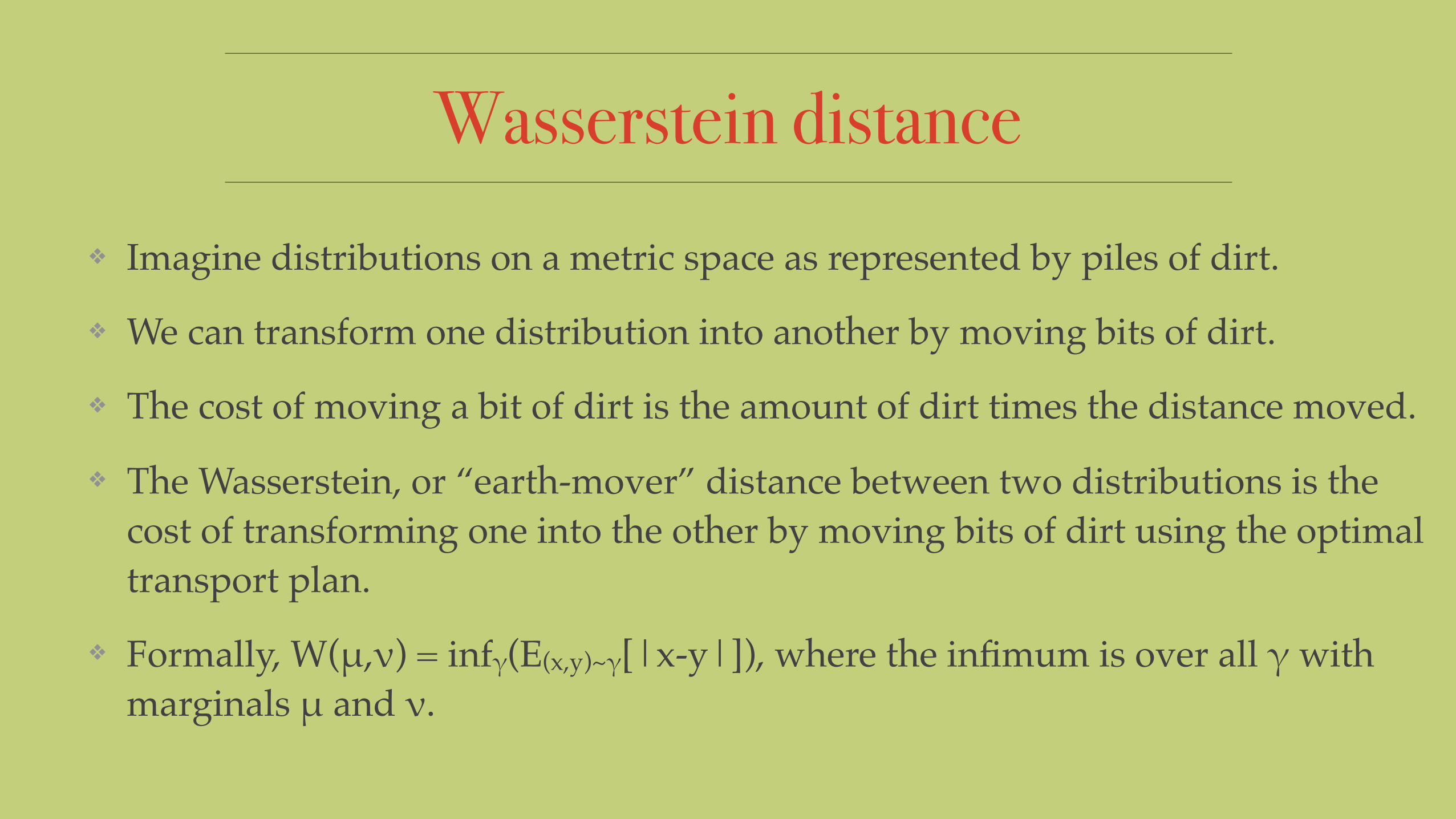
Wasserstein distance❖ Imagine distributions on a metric space as represented by piles of dirt.
❖ We can transform one distribution into another by moving bits of dirt.
❖ The cost of moving a bit of dirt is the amount of dirt times the distance moved.
❖ The Wasserstein, or “earth-mover” distance between two distributions is the cost of transforming one into the other by moving bits of dirt using the optimal transport plan.
❖ Formally, W(μ,ν) = infγ(E(x,y)~γ[|x-y|]), where the infimum is over all γ with marginals μ and ν.
Wasserstein Distance (cont’d)
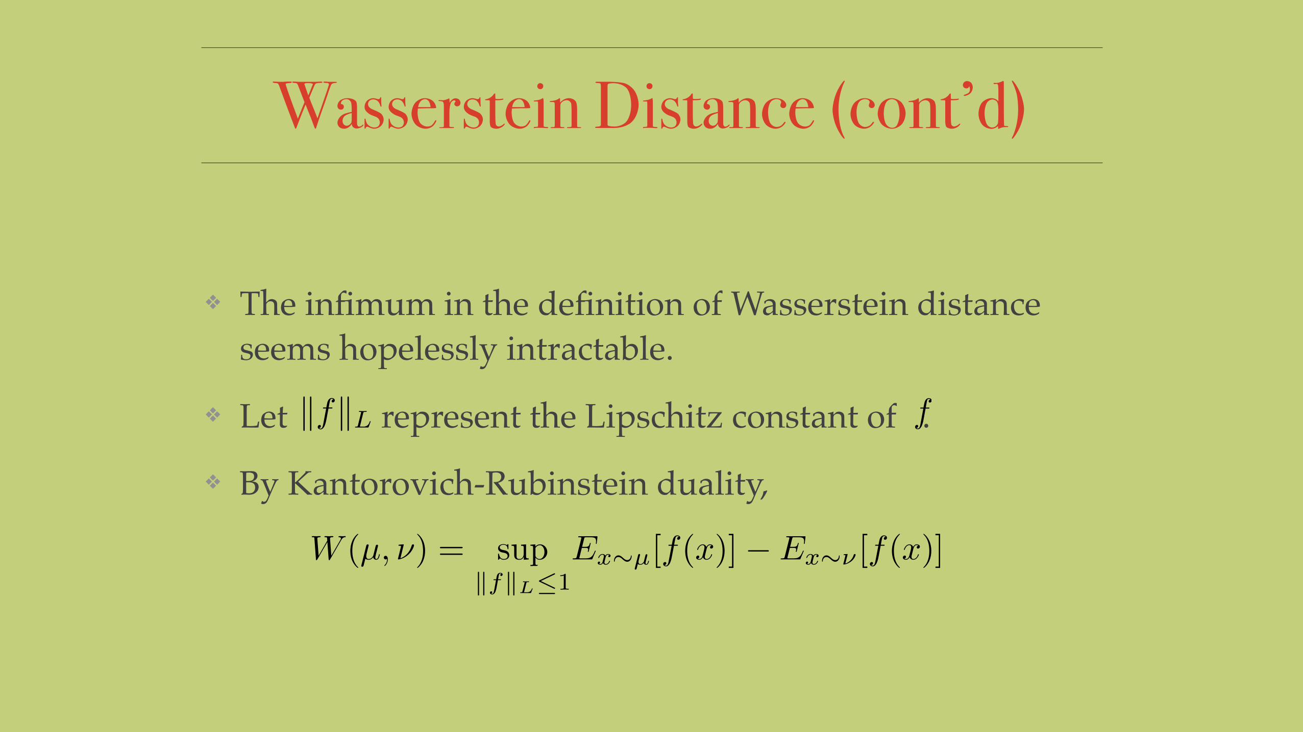
❖ The infimum in the definition of Wasserstein distance seems hopelessly intractable.
❖ Let represent the Lipschitz constant of .
❖ By Kantorovich-Rubinstein duality,
W (µ, ⌫) = supkfkL1
E
x⇠µ
[f(x)]� E
x⇠⌫
[f(x)]
kfkL f

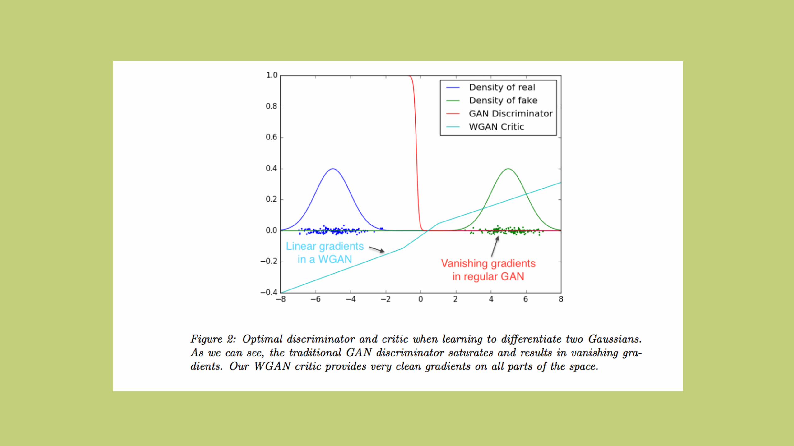
Wasserstein Distance (cont’d)❖ Blue and green are the pdfs of a gaussian and a
mixture of two gaussians.
❖ Red is the optimal f for Kantorovich-Rubinstein duality, computed using ADAM, scaled by a factor of 1/25 to fit nicely on the graph, mean arbitrarily fixed at 0.
❖ Note that the slope of f always has absolute value 1. You can prove this is basically always true.
❖ (At the extreme right of the graph, what happens is just that ADAM can’t optimize because the two pdfs are both practically zero.)
❖ The bottom plot additionally shows the product of f with the difference in the pdfs (which is being minimized).

Wasserstein Distance (cont’d)❖ The discriminator (or “critic”) will approximate the Wasserstein distance if we
train it to maximize not Ex~q[log(D(x))] + Ez~p[log(1-D(G(z)))] but Ex~q[D(x)] - Ez~p[D(G(z))]…
❖ … so long as we can somehow constrain it to be 1-Lipschitz (or K-Lipschitz for some K since different K will just give scaled versions of Wasserstein distance, which will have the same convergence properties).
❖ Wasserstein GANs suggests doing this by limiting how big the weights can be (“weight clipping”). They suggest absolute value .01.
❖ Had to switch from ADAM to RMSProp as critic optimizer.

Wasserstein GAN results
❖ It is now possible and desirable to train the critic to optimality.
❖ You get a meaningful loss function.
❖ Training is more stable.
❖ Mode dropping is greatly reduced.
❖ (Note that Mode Chasing is not directly addressed. But I think that since the discriminator can be kept near its optimum, it should be reduced, both because the discriminator will be more constant on the data distribution and because the modes will change more rapidly from the perspective of the generator.)


Improved Training of Wasserstein GANs
❖ Weight clipping has a massive problem: it only searches over a small subset of k-Lipschitz functions.
❖ In particular, the optimal critic under WGAN loss would have gradient of norm one almost everywhere.
❖ But under a weight-clipping constraint, most neural network architectures can only have norm one almost everywhere when they compute extremely simple functions, severely underusing their capacity.


Improved Training of Wasserstein GANs (cont’d)
❖ Another problem the paper identifies with weight clipping is that it leads to vanishing and exploding gradients, which can only be partly mitigated using batch norm.

Improved Training of Wasserstein GANs (cont’d)
❖ Not only does the optimal critic have gradient norm one almost everywhere, but having gradient norm less than or equal to one almost everywhere is equivalent to being 1-Lipschitz and differentiable.
❖ So a good way to enforce the 1-Lipschitz constraint would be to penalize the critic for having a gradient norm that differs from one.
❖ (Actually, enforcing this constraint everywhere is intractable, so they approximate by enforcing it at points sampled on lines between generator samples and data samples.)

Improved Training of Wasserstein GANs (results)
❖ No batch norm necessary in critic (good not only because batch norm takes resources but also because it is harder to understand GAN dynamics in its presence).
❖ Can use ADAM again (or, presumably, SGD with momentum).
❖ Greater stability of training.
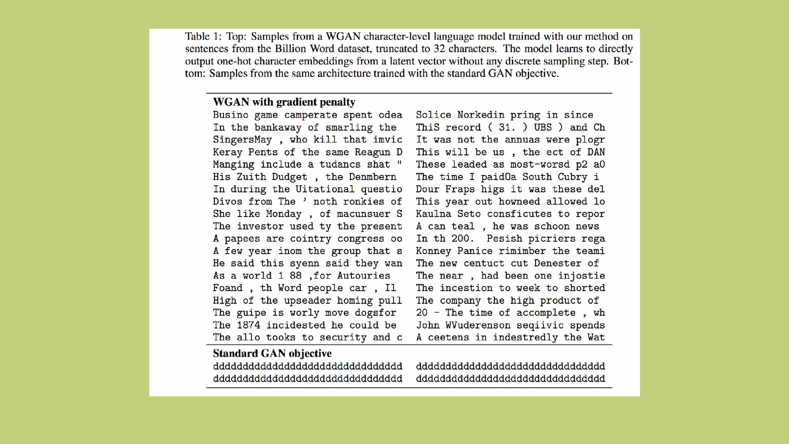
❖ They demonstrate that Wasserstein GANs can produce discrete output by simply passing a softmax output directly to the critic(!). (However, it is too early to tell if this technique will be the end of discrete output problems for GANs.)


A Tiny Bit on BEGAN


Thank You!❖ Standard value function: V(G,D) = Ex~q[log(D(x))] +
Ez~p[log(1-D(G(z)))]
❖ Wasserstein GAN value function: V(G,D) = Ex~q[D(x)] - Ez~p[D(G(z))]
❖ Hacky generator objective: log(D(G(z)))
❖ Minimax objective: minG maxD V(G,D)
❖ Wasserstein distance: W(μ,ν) = infγ(E(x, y)~γ[|x-y|])
❖ Dual form: W (µ, ⌫) = supkfkL1
E
x⇠µ
[f(x)]� E
x⇠⌫
[f(x)]