introduction to functional programming · preface these are the lecture notes accompanying the...
TRANSCRIPT


i
Preface
These are the lecture notes accompanying the course Introduction to FunctionalProgramming, which I taught at Cambridge University in the academic year1996/7.
This course has mainly been taught in previous years by Mike Gordon. I haveretained the basic structure of his course, with a blend of theory and practice,and have borrowed heavily in what follows from his own lecture notes, availablein book form as Part II of (Gordon 1988). I have also been influenced by thosewho have taught related courses here, such as Andy Gordon and Larry Paulsonand, in the chapter on types, by Andy Pitts’s course on the subject.
The large chapter on examples is not directly examinable, though studying itshould improve the reader’s grasp of the early parts and give a better idea abouthow ML is actually used.
Most chapters include some exercises, either invented specially for this courseor taken from various sources. They are normally intended to require a littlethought, rather than just being routine drill. Those I consider fairly difficult aremarked with a (*).
These notes have not yet been tested extensively and no doubt contain variouserrors and obscurities. I would be grateful for constructive criticism from anyreaders.
John Harrison ([email protected]).
ii

Plan of the lectures
This chapter indicates roughly how the material is to be distributed over a courseof twelve lectures, each of slightly less than one hour.
1. Introduction and Overview Functional and imperative programming:contrast, pros and cons. General structure of the course: how lambda cal-culus turns out to be a general programming language. Lambda notation:how it clarifies variable binding and provides a general analysis of mathe-matical notation. Currying. Russell’s paradox.
2. Lambda calculus as a formal system Free and bound variables. Sub-stitution. Conversion rules. Lambda equality. Extensionality. Reductionand reduction strategies. The Church-Rosser theorem: statement and con-sequences. Combinators.
3. Lambda calculus as a programming language Computability back-ground; Turing completeness (no proof). Representing data and basic op-erations: truth values, pairs and tuples, natural numbers. The predecessoroperation. Writing recursive functions: fixed point combinators. Let ex-pressions. Lambda calculus as a declarative language.
4. Types Why types? Answers from programming and logic. Simply typedlambda calculus. Church and Curry typing. Let polymorphism. Mostgeneral types and Milner’s algorithm. Strong normalization (no proof),and its negative consequences for Turing completeness. Adding a recursionoperator.
5. ML ML as typed lambda calculus with eager evaluation. Details of evalu-ation strategy. The conditional. The ML family. Practicalities of interact-ing with ML. Writing functions. Bindings and declarations. Recursive andpolymorphic functions. Comparison of functions.
6. Details of ML More about interaction with ML. Loading from files. Com-ments. Basic data types: unit, booleans, numbers and strings. Built-inoperations. Concrete syntax and infixes. More examples. Recursive typesand pattern matching. Examples: lists and recursive functions on lists.
iii
iv
7. Proving programs correct The correctness problem. Testing and veri-fication. The limits of verification. Functional programs as mathematicalobjects. Examples of program proofs: exponential, GCD, append and re-verse.
8. Effective ML Using standard combinators. List iteration and other usefulcombinators; examples. Tail recursion and accumulators; why tail recursionis more efficient. Forcing evaluation. Minimizing consing. More efficientreversal. Use of ‘as’. Imperative features: exceptions, references, arraysand sequencing. Imperative features and types; the value restriction.
9. ML examples I: symbolic differentiation Symbolic computation. Datarepresentation. Operator precedence. Association lists. Prettyprintingexpressions. Installing the printer. Differentiation. Simplification. Theproblem of the ‘right’ simplification.
10. ML examples II: recursive descent parsing Grammars and the parsingproblem. Fixing ambiguity. Recursive descent. Parsers in ML. Parsercombinators; examples. Lexical analysis using the same techniques. Aparser for terms. Automating precedence parsing. Avoiding backtracking.Comparison with other techniques.
11. ML examples III: exact real arithmetic Real numbers and finite repre-sentations. Real numbers as programs or functions. Our representation ofreals. Arbitrary precision integers. Injecting integers into the reals. Nega-tion and absolute value. Addition; the importance of rounding division.Multiplication and division by integers. General multiplication. Inverse anddivision. Ordering and equality. Testing. Avoiding reevaluation throughmemo functions.
12. ML examples IV: Prolog and theorem proving Prolog terms. Case-sensitive lexing. Parsing and printing, including list syntax. Unification.Backtracking search. Prolog examples. Prolog-style theorem proving. Ma-nipulating formulas; negation normal form. Basic prover; the use of con-tinuations. Examples: Pelletier problems and whodunit.

Contents
1 Introduction 11.1 The merits of functional programming . . . . . . . . . . . . . . . 31.2 Outline . . . . . . . . . . . . . . . . . . . . . . . . . . . . . . . . . 5
2 Lambda calculus 72.1 The benefits of lambda notation . . . . . . . . . . . . . . . . . . . 82.2 Russell’s paradox . . . . . . . . . . . . . . . . . . . . . . . . . . . 112.3 Lambda calculus as a formal system . . . . . . . . . . . . . . . . . 12
2.3.1 Lambda terms . . . . . . . . . . . . . . . . . . . . . . . . . 122.3.2 Free and bound variables . . . . . . . . . . . . . . . . . . . 132.3.3 Substitution . . . . . . . . . . . . . . . . . . . . . . . . . . 142.3.4 Conversions . . . . . . . . . . . . . . . . . . . . . . . . . . 162.3.5 Lambda equality . . . . . . . . . . . . . . . . . . . . . . . 162.3.6 Extensionality . . . . . . . . . . . . . . . . . . . . . . . . . 172.3.7 Lambda reduction . . . . . . . . . . . . . . . . . . . . . . 182.3.8 Reduction strategies . . . . . . . . . . . . . . . . . . . . . 192.3.9 The Church-Rosser theorem . . . . . . . . . . . . . . . . . 19
2.4 Combinators . . . . . . . . . . . . . . . . . . . . . . . . . . . . . . 21
3 Lambda calculus as a programming language 243.1 Representing data in lambda calculus . . . . . . . . . . . . . . . . 26
3.1.1 Truth values and the conditional . . . . . . . . . . . . . . 263.1.2 Pairs and tuples . . . . . . . . . . . . . . . . . . . . . . . . 273.1.3 The natural numbers . . . . . . . . . . . . . . . . . . . . . 29
3.2 Recursive functions . . . . . . . . . . . . . . . . . . . . . . . . . . 313.3 Let expressions . . . . . . . . . . . . . . . . . . . . . . . . . . . . 333.4 Steps towards a real programming language . . . . . . . . . . . . 353.5 Further reading . . . . . . . . . . . . . . . . . . . . . . . . . . . . 36
4 Types 384.1 Typed lambda calculus . . . . . . . . . . . . . . . . . . . . . . . . 39
4.1.1 The stock of types . . . . . . . . . . . . . . . . . . . . . . 404.1.2 Church and Curry typing . . . . . . . . . . . . . . . . . . 41
v
vi CONTENTS
4.1.3 Formal typability rules . . . . . . . . . . . . . . . . . . . . 424.1.4 Type preservation . . . . . . . . . . . . . . . . . . . . . . . 43
4.2 Polymorphism . . . . . . . . . . . . . . . . . . . . . . . . . . . . . 444.2.1 Let polymorphism . . . . . . . . . . . . . . . . . . . . . . 454.2.2 Most general types . . . . . . . . . . . . . . . . . . . . . . 46
4.3 Strong normalization . . . . . . . . . . . . . . . . . . . . . . . . . 47
5 A taste of ML 505.1 Eager evaluation . . . . . . . . . . . . . . . . . . . . . . . . . . . 505.2 Consequences of eager evaluation . . . . . . . . . . . . . . . . . . 535.3 The ML family . . . . . . . . . . . . . . . . . . . . . . . . . . . . 545.4 Starting up ML . . . . . . . . . . . . . . . . . . . . . . . . . . . . 545.5 Interacting with ML . . . . . . . . . . . . . . . . . . . . . . . . . 555.6 Bindings and declarations . . . . . . . . . . . . . . . . . . . . . . 565.7 Polymorphic functions . . . . . . . . . . . . . . . . . . . . . . . . 585.8 Equality of functions . . . . . . . . . . . . . . . . . . . . . . . . . 60
6 Further ML 636.1 Basic datatypes and operations . . . . . . . . . . . . . . . . . . . 646.2 Syntax of ML phrases . . . . . . . . . . . . . . . . . . . . . . . . 666.3 Further examples . . . . . . . . . . . . . . . . . . . . . . . . . . . 686.4 Type definitions . . . . . . . . . . . . . . . . . . . . . . . . . . . . 70
6.4.1 Pattern matching . . . . . . . . . . . . . . . . . . . . . . . 716.4.2 Recursive types . . . . . . . . . . . . . . . . . . . . . . . . 736.4.3 Tree structures . . . . . . . . . . . . . . . . . . . . . . . . 766.4.4 The subtlety of recursive types . . . . . . . . . . . . . . . 78
7 Proving programs correct 817.1 Functional programs as mathematical objects . . . . . . . . . . . 837.2 Exponentiation . . . . . . . . . . . . . . . . . . . . . . . . . . . . 847.3 Greatest common divisor . . . . . . . . . . . . . . . . . . . . . . . 857.4 Appending . . . . . . . . . . . . . . . . . . . . . . . . . . . . . . . 867.5 Reversing . . . . . . . . . . . . . . . . . . . . . . . . . . . . . . . 87
8 Effective ML 948.1 Useful combinators . . . . . . . . . . . . . . . . . . . . . . . . . . 948.2 Writing efficient code . . . . . . . . . . . . . . . . . . . . . . . . . 96
8.2.1 Tail recursion and accumulators . . . . . . . . . . . . . . . 968.2.2 Minimizing consing . . . . . . . . . . . . . . . . . . . . . . 988.2.3 Forcing evaluation . . . . . . . . . . . . . . . . . . . . . . 101
8.3 Imperative features . . . . . . . . . . . . . . . . . . . . . . . . . . 1028.3.1 Exceptions . . . . . . . . . . . . . . . . . . . . . . . . . . . 1028.3.2 References and arrays . . . . . . . . . . . . . . . . . . . . . 104

CONTENTS vii
8.3.3 Sequencing . . . . . . . . . . . . . . . . . . . . . . . . . . 1058.3.4 Interaction with the type system . . . . . . . . . . . . . . 106
9 Examples 1099.1 Symbolic differentiation . . . . . . . . . . . . . . . . . . . . . . . 109
9.1.1 First order terms . . . . . . . . . . . . . . . . . . . . . . . 1109.1.2 Printing . . . . . . . . . . . . . . . . . . . . . . . . . . . . 1109.1.3 Derivatives . . . . . . . . . . . . . . . . . . . . . . . . . . 1149.1.4 Simplification . . . . . . . . . . . . . . . . . . . . . . . . . 115
9.2 Parsing . . . . . . . . . . . . . . . . . . . . . . . . . . . . . . . . . 1189.2.1 Recursive descent parsing . . . . . . . . . . . . . . . . . . 1209.2.2 Parser combinators . . . . . . . . . . . . . . . . . . . . . . 1209.2.3 Lexical analysis . . . . . . . . . . . . . . . . . . . . . . . . 1229.2.4 Parsing terms . . . . . . . . . . . . . . . . . . . . . . . . . 1239.2.5 Automatic precedence parsing . . . . . . . . . . . . . . . . 1249.2.6 Defects of our approach . . . . . . . . . . . . . . . . . . . 126
9.3 Exact real arithmetic . . . . . . . . . . . . . . . . . . . . . . . . . 1289.3.1 Representation of real numbers . . . . . . . . . . . . . . . 1299.3.2 Arbitrary-precision integers . . . . . . . . . . . . . . . . . 1299.3.3 Basic operations . . . . . . . . . . . . . . . . . . . . . . . 1319.3.4 General multiplication . . . . . . . . . . . . . . . . . . . . 1359.3.5 Multiplicative inverse . . . . . . . . . . . . . . . . . . . . . 1369.3.6 Ordering relations . . . . . . . . . . . . . . . . . . . . . . . 1389.3.7 Caching . . . . . . . . . . . . . . . . . . . . . . . . . . . . 138
9.4 Prolog and theorem proving . . . . . . . . . . . . . . . . . . . . . 1419.4.1 Prolog terms . . . . . . . . . . . . . . . . . . . . . . . . . 1429.4.2 Lexical analysis . . . . . . . . . . . . . . . . . . . . . . . . 1429.4.3 Parsing . . . . . . . . . . . . . . . . . . . . . . . . . . . . 1439.4.4 Unification . . . . . . . . . . . . . . . . . . . . . . . . . . . 1449.4.5 Backtracking . . . . . . . . . . . . . . . . . . . . . . . . . 1469.4.6 Examples . . . . . . . . . . . . . . . . . . . . . . . . . . . 1479.4.7 Theorem proving . . . . . . . . . . . . . . . . . . . . . . . 149

Chapter 1
Introduction
Programs in traditional languages, such as FORTRAN, Algol, C and Modula-3,rely heavily on modifying the values of a collection of variables, called the state. Ifwe neglect the input-output operations and the possibility that a program mightrun continuously (e.g. the controller for a manufacturing process), we can arriveat the following abstraction. Before execution, the state has some initial valueσ, representing the inputs to the program, and when the program has finished,the state has a new value σ′ including the result(s). Moreover, during execution,each command changes the state, which has therefore proceeded through somefinite sequence of values:
σ = σ0 → σ1 → σ2 → · · · → σn = σ′
For example in a sorting program, the state initially includes an array ofvalues, and when the program has finished, the state has been modified in such away that these values are sorted, while the intermediate states represent progresstowards this goal.
The state is typically modified by assignment commands, often written inthe form v = E or v := E where v is a variable and E some expression. Thesecommands can be executed in a sequential manner by writing them one after theother in the program, often separated by a semicolon. By using statements likeif and while, one can execute these commands conditionally, and repeatedly,depending on other properties of the current state. The program amounts to a setof instructions on how to perform these state changes, and therefore this style ofprogramming is often called imperative or procedural. Correspondingly, the tra-ditional languages intended to support it are known as imperative or procedurallanguages.
Functional programming represents a radical departure from this model. Es-sentially, a functional program is simply an expression, and execution meansevaluation of the expression.1 We can see how this might be possible, in gen-
1Functional programming is often called ‘applicative programming’ since the basic mecha-
1
2 CHAPTER 1. INTRODUCTION
eral terms, as follows. Assuming that an imperative program (as a whole) isdeterministic, i.e. the output is completely determined by the input, we can saythat the final state, or whichever fragments of it are of interest, is some func-tion of the initial state, say σ′ = f(σ).2 In functional programming this viewis emphasized: the program is actually an expression that corresponds to themathematical function f . Functional languages support the construction of suchexpressions by allowing rather powerful functional constructs.
Functional programming can be contrasted with imperative programming ei-ther in a negative or a positive sense. Negatively, functional programs do notuse variables — there is no state. Consequently, they cannot use assignments,since there is nothing to assign to. Furthermore the idea of executing commandsin sequence is meaningless, since the first command can make no difference tothe second, there being no state to mediate between them. Positively however,functional programs can use functions in much more sophisticated ways. Func-tions can be treated in exactly the same way as simpler objects like integers: theycan be passed to other functions as arguments and returned as results, and ingeneral calculated with. Instead of sequencing and looping, functional languagesuse recursive functions, i.e. functions that are defined in terms of themselves. Bycontrast, most traditional languages provide poor facilities in these areas. C al-lows some limited manipulation of functions via pointers, but does not allow oneto create new functions dynamically. FORTRAN does not even support recursionat all.
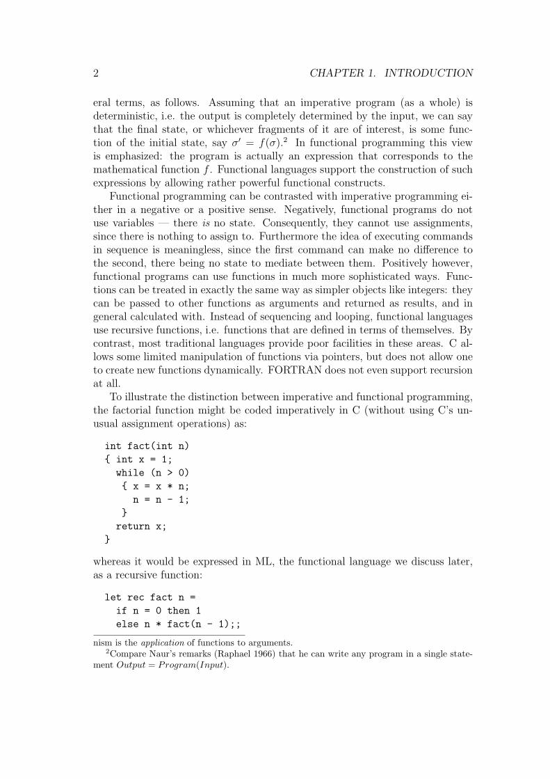
To illustrate the distinction between imperative and functional programming,the factorial function might be coded imperatively in C (without using C’s un-usual assignment operations) as:
int fact(int n)
{ int x = 1;
while (n > 0)
{ x = x * n;
n = n - 1;
}
return x;
}
whereas it would be expressed in ML, the functional language we discuss later,as a recursive function:
let rec fact n =
if n = 0 then 1
else n * fact(n - 1);;
nism is the application of functions to arguments.2Compare Naur’s remarks (Raphael 1966) that he can write any program in a single state-
ment Output = Program(Input).
1.1. THE MERITS OF FUNCTIONAL PROGRAMMING 3
In fact, this sort of definition can be used in C too. However for more sophis-ticated uses of functions, functional languages stand in a class by themselves.
1.1 The merits of functional programming
At first sight, a language without variables or sequencing might seem completelyimpractical. This impression cannot be dispelled simply by a few words here.But we hope that by studying the material that follows, readers will gain anappreciation of how it is possible to do a lot of interesting programming in thefunctional manner.
There is nothing sacred about the imperative style, familiar though it is.Many features of imperative languages have arisen by a process of abstractionfrom typical computer hardware, from machine code to assemblers, to macro as-semblers, and then to FORTRAN and beyond. There is no reason to supposethat such languages represent the most palatable way for humans to communi-cate programs to a machine. After all, existing hardware designs are not sacredeither, and computers are supposed to do our bidding rather than conversely.Perhaps the right approach is not to start from the hardware and work upwards,but to start with programming languages as an abstract notation for specifyingalgorithms, and then work down to the hardware (Dijkstra 1976). Actually, thistendency can be detected in traditional languages too. Even FORTRAN allowsarithmetical expressions to be written in the usual way. The programmer is notburdened with the task of linearizing the evaluation of subexpressions and findingtemporary storage for intermediate results.
This suggests that the idea of developing programming languages quite dif-ferent from the traditional imperative ones is certainly defensible. However, toemphasize that we are not merely proposing change for change’s sake, we shouldsay a few words about why we might prefer functional programs to imperativeones.
Perhaps the main reason is that functional programs correspond more directlyto mathematical objects, and it is therefore easier to reason about them. In orderto get a firm grip on exactly what programs mean, we might wish to assign anabstract mathematical meaning to a program or command — this is the aimof denotational semantics (semantics = meaning). In imperative languages, thishas to be done in a rather indirect way, because of the implicit dependencyon the value of the state. In simple imperative languages, one can associatea command with a function Σ → Σ, where Σ is the set of possible values forthe state. That is, a command takes some state and produces another state.It may fail to terminate (e.g. while true do x := x), so this function mayin general be partial. Alternative semantics are sometimes preferred, e.g. interms of predicate transformers (Dijkstra 1976). But if we add features that canpervert the execution sequence in more complex ways, e.g. goto, or C’s break
4 CHAPTER 1. INTRODUCTION
and continue, even these interpretations no longer work, since one commandcan cause the later commands to be skipped. Instead, one typically uses a morecomplicated semantics based on continuations.
By contrast functional programs, in the words of Henson (1987), ‘wear theirsemantics on their sleeves’.3 We can illustrate this using ML. The basic datatypeshave a direct interpretation as mathematical objects. Using the standard notationof [[X]] for ‘the semantics of X’, we can say for example that [[int]] = Z. Now theML function fact defined by:
let rec fact n =
if n = 0 then 1
else n * fact(n - 1);;
has one argument of type int, and returns a value of type int, so it can simplybe associated with an abstract partial function Z → Z:
[[fact]](n) =
{n! if n ≥ 0⊥ otherwise
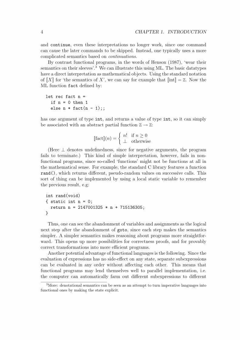
(Here ⊥ denotes undefinedness, since for negative arguments, the programfails to terminate.) This kind of simple interpretation, however, fails in non-functional programs, since so-called ‘functions’ might not be functions at all inthe mathematical sense. For example, the standard C library features a functionrand(), which returns different, pseudo-random values on successive calls. Thissort of thing can be implemented by using a local static variable to rememberthe previous result, e.g:
int rand(void)
{ static int n = 0;
return n = 2147001325 * n + 715136305;
}
Thus, one can see the abandonment of variables and assignments as the logicalnext step after the abandonment of goto, since each step makes the semanticssimpler. A simpler semantics makes reasoning about programs more straightfor-ward. This opens up more possibilities for correctness proofs, and for provablycorrect transformations into more efficient programs.
Another potential advantage of functional languages is the following. Since theevaluation of expressions has no side-effect on any state, separate subexpressionscan be evaluated in any order without affecting each other. This means thatfunctional programs may lend themselves well to parallel implementation, i.e.the computer can automatically farm out different subexpressions to different
3More: denotational semantics can be seen as an attempt to turn imperative languages intofunctional ones by making the state explicit.
1.2. OUTLINE 5
processors. By contrast, imperative programs often impose a fairly rigid order ofexecution, and even the limited interleaving of instructions in modern pipelinedprocessors turns out to be complicated and full of technical problems.
Actually, ML is not a purely functional programming language; it does havevariables and assignments if required. Most of the time, we will work inside thepurely functional subset. But even if we do use assignments, and lose some of thepreceding benefits, there are advantages too in the more flexible use of functionsthat languages like ML allow. Programs can often be expressed in a very conciseand elegant style using higher-order functions (functions that operate on otherfunctions).4 Code can be made more general, since it can be parametrized evenover other functions. For example, a program to add up a list of numbers and aprogram to multiply a list of numbers can be seen as instances of the same pro-gram, parametrized by the pairwise arithmetic operation and the correspondingidentity. In one case it is given + and 0 and in the other case, ∗ and 1.5 Finally,functions can also be used to represent infinite data in a convenient way — forexample we will show later how to use functions to perform exact calculationwith real numbers, as distinct from floating point approximations.
At the same time, functional programs are not without their problems. Sincethey correspond less directly the the eventual execution in hardware, it can bedifficult to reason about their exact usage of resources such as time and space.Input-output is also difficult to incorporate neatly into a functional model, thoughthere are ingenious techniques based on infinite sequences.
It is up to readers to decide, after reading this book, on the merits of thefunctional style. We do not wish to enforce any ideologies, merely to point outthat there are different ways of looking at programming, and that in the rightsituations, functional programming may have considerable merits. Most of ourexamples are chosen from areas that might loosely be described as ‘symboliccomputation’, for we believe that functional programs work well in such appli-cations. However, as always one should select the most appropriate tool for thejob. It may be that imperative programming, object-oriented programming orlogic programming are more suited to certain tasks. Horses for courses.
1.2 Outline
For those used to imperative programming, the transition to functional program-ming is inevitably difficult, whatever approach is taken. While some will be im-
4Elegance is subjective and conciseness is not an end in itself. Functional languages, andother languages like APL, often create a temptation to produce very short tricky code whichis elegant to cognoscenti but obscure to outsiders.
5This parallels the notion of abstraction in pure mathematics, e.g. that the additive andmultiplicative structures over numbers are instances of the abstract notion of a monoid. Thissimilarly avoids duplication and increases elegance.
6 CHAPTER 1. INTRODUCTION
patient to get quickly to real programming, we have chosen to start with lambdacalculus, and show how it can be seen as the theoretical underpinning for func-tional languages. This has the merit of corresponding quite well to the actualhistorical line of development.
So first we introduce lambda calculus, and show how what was originallyintended as a formal logical system for mathematics turned out to be a completelygeneral programming language. We then discuss why we might want to add typesto lambda calculus, and show how it can be done. This leads us into ML, which isessentially an extended and optimized implementation of typed lambda calculuswith a certain evaluation strategy. We cover the practicalities of basic functionalprogramming in ML, and discuss polymorphism and most general types. Wethen move on to more advanced topics including exceptions and ML’s imperativefeatures. We conclude with some substantial examples, which we hope provideevidence for the power of ML.
Further reading
Numerous textbooks on ‘functional programming’ include a general introductionto the field and a contrast with imperative programming — browse through afew and find one that you like. For example, Henson (1987) contains a goodintroductory discussion, and features a similar mixture of theory and practiceto this text. A detailed and polemical advocacy of the functional style is givenby Backus (1978), the main inventor of FORTRAN. Gordon (1994) discusses theproblems of incorporating input-output into functional languages, and some solu-tions. Readers interested in denotational semantics, for imperative and functionallanguages, may look at Winskel (1993).
Chapter 2
Lambda calculus
Lambda calculus is based on the so-called ‘lambda notation’ for denoting func-tions. In informal mathematics, when one wants to refer to a function, one usuallyfirst gives the function an arbitrary name, and thereafter uses that name, e.g.
Suppose f : R → R is defined by:
f(x) =
{0 if x = 0x2sin(1/x2) if x 6= 0
Then f ′(x) is not Lebesgue integrable over the unit interval [0, 1].
Most programming languages, C for example, are similar in this respect: wecan define functions only by giving them names. For example, in order to usethe successor function (which adds 1 to its argument) in nontrivial ways (e.g.consider a pointer to it), then even though it is very simple, we need to name itvia some function definition such as:
int suc(int n)
{ return n + 1;
}
In either mathematics or programming, this seems quite natural, and gener-ally works well enough. However it can get clumsy when higher order functions(functions that manipulate other functions) are involved. In any case, if we wantto treat functions on a par with other mathematical objects, the insistence onnaming is rather inconsistent. When discussing an arithmetical expression builtup from simpler ones, we just write the subexpressions down, without needing togive them names. Imagine if we always had to deal with arithmetic expressionsin this way:
Define x and y by x = 2 and y = 4 respectively. Then xx = y.
7

8 CHAPTER 2. LAMBDA CALCULUS
Lambda notation allows one to denote functions in much the same way as anyother sort of mathematical object. There is a mainstream notation sometimesused in mathematics for this purpose, though it’s normally still used as part ofthe definition of a temporary name. We can write
x 7→ t[x]
to denote the function mapping any argument x to some arbitrary expression t[x],which usually, but not necessarily, contains x (it is occasionally useful to “throwaway” an argument). However, we shall use a different notation developed byChurch (1941):
λx. t[x]
which should be read in the same way. For example, λx.x is the identity functionwhich simply returns its argument, while λx. x2 is the squaring function.
The symbol λ is completely arbitrary, and no significance should be read intoit. (Indeed one often sees, particularly in French texts, the alternative notation[x] t[x].) Apparently it arose by a complicated process of evolution. Originally,the famous Principia Mathematica (Whitehead and Russell 1910) used the ‘hat’notation t[x] for the function of x yielding t[x]. Church modified this to x. t[x],but since the typesetter could not place the hat on top of the x, this appeared as∧x. t[x], which then mutated into λx. t[x] in the hands of another typesetter.
2.1 The benefits of lambda notation
Using lambda notation we can clear up some of the confusion engendered byinformal mathematical notation. For example, it’s common to talk sloppily about‘f(x)’, leaving context to determine whether we mean f itself, or the result ofapplying it to particular x. A further benefit is that lambda notation givesan attractive analysis of practically the whole of mathematical notation. If westart with variables and constants, and build up expressions using just lambda-abstraction and application of functions to arguments, we can represent verycomplicated mathematical expressions.
We will use the conventional notation f(x) for the application of a function fto an argument x, except that, as is traditional in lambda notation, the bracketsmay be omitted, allowing us to write just f x. For reasons that will becomeclear in the next paragraph, we assume that function application associates tothe left, i.e. f x y means (f(x))(y). As a shorthand for λx. λy. t[x, y] we will useλx y. t[x, y], and so on. We also assume that the scope of a lambda abstractionextends as far to the right as possible. For example λx.x y means λx.(x y) ratherthan (λx. x) y.

2.1. THE BENEFITS OF LAMBDA NOTATION 9
At first sight, we need some special notation for functions of several arguments.However there is a way of breaking down such applications into ordinary lambdanotation, called currying, after the logician Curry (1930). (Actually the devicehad previously been used by both Frege (1893) and Schonfinkel (1924), but it’seasy to understand why the corresponding appellations haven’t caught the publicimagination.) The idea is to use expressions like λx y. x + y. This may beregarded as a function R → (R → R), so it is said to be a ‘higher order function’or ‘functional’ since when applied to one argument, it yields another function,which then accepts the second argument. In a sense, it takes its arguments oneat a time rather than both together. So we have for example:
(λx y. x + y) 1 2 = (λy. 1 + y) 2 = 1 + 2
Observe that function application is assumed to associate to the left in lambdanotation precisely because currying is used so much.
Lambda notation is particularly helpful in providing a unified treatment ofbound variables. Variables in mathematics normally express the dependency ofsome expression on the value of that variable; for example, the value of x2 + 2depends on the value of x. In such contexts, we will say that a variable is free.However there are other situations where a variable is merely used as a place-marker, and does not indicate such a dependency. Two common examples arethe variable m in
n∑m=1
m =n(n + 1)
2
and the variable y in ∫ x
02y + a dy = x2 + ax
In logic, the quantifiers ∀x. P [x] (‘for all x, P [x]’) and ∃x. P [x] (‘there existsan x such that P [x]’) provide further examples, and in set theory we have setabstractions like {x | P [x]} as well as indexed unions and intersections. In suchcases, a variable is said to be bound. In a certain subexpression it is free, but inthe whole expression, it is bound by a variable-binding operation like summation.The part ‘inside’ this variable-binding operation is called the scope of the boundvariable.
A similar situation occurs in most programming languages, at least from Algol60 onwards. Variables have a definite scope, and the formal arguments of proce-dures and functions are effectively bound variables, e.g. n in the C definition ofthe successor function given above. One can actually regard variable declarationsas binding operations for the enclosed instances of the corresponding variable(s).Note, by the way, that the scope of a variable should be distinguished sharplyfrom its lifetime. In the C function rand that we gave in the introduction, n had

10 CHAPTER 2. LAMBDA CALCULUS
a textually limited scope but it retained its value even outside the execution ofthat part of the code.
We can freely change the name of a bound variable without changing themeaning of the expression, e.g.∫ x
02z + a dz = x2 + ax
Similarly, in lambda notation, λx. E[x] and λy. E[y] are equivalent; this iscalled alpha-equivalence and the process of transforming between such pairs iscalled alpha-conversion. We should add the proviso that y is not a free variablein E[x], or the meaning clearly may change, just as∫ x
02a + a da 6= x2 + ax
It is possible to have identically-named free and bound variables in the sameexpression; though this can be confusing, it is technically unambiguous, e.g.∫ x
02x + a dx = x2 + ax
In fact the usual Leibniz notation for derivatives has just this property, e.g. in:
d
dxx2 = 2x
x is used both as a bound variable to indicate that differentiation is to takeplace with respect to x, and as a free variable to show where to evaluate theresulting derivative. This can be confusing; e.g. f ′(g(x)) is usually taken to meansomething different from d
dxf(g(x)). Careful writers, especially in multivariate
work, often make the separation explicit by writing:
| d
dxx2|x = 2x
or
| d
dzz2|x = 2x
Part of the appeal of lambda notation is that all variable-binding opera-tions like summation, differentiation and integration can be regarded as func-tions applied to lambda-expressions. Subsuming all variable-binding operationsby lambda abstraction allows us to concentrate on the technical problems ofbound variables in one particular situation. For example, we can view d
dxx2 as
a syntactic sugaring of D (λx. x2) x where D : (R → R) → R → R is a dif-ferentiation operator, yielding the derivative of its first (function) argument atthe point indicated by its second argument. Breaking down the everyday syntaxcompletely into lambda notation, we have D (λx. EXP x 2) x for some constantEXP representing the exponential function.

2.2. RUSSELL’S PARADOX 11
In this way, lambda notation is an attractively general ‘abstract syntax’ formathematics; all we need is the appropriate stock of constants to start with.Lambda abstraction seems, in retrospect, to be the appropriate primitive in termsof which to analyze variable binding. This idea goes back to Church’s encodingof higher order logic in lambda notation, and as we shall see in the next chapter,Landin has pointed out how many constructs from programming languages havea similar interpretation. In recent times, the idea of using lambda notation asa universal abstract syntax has been put especially clearly by Martin-Lof, andis often referred to in some circles as ‘Martin-Lof’s theory of expressions andarities’.1
2.2 Russell’s paradox
As we have said, one of the appeals of lambda notation is that it permits ananalysis of more or less all of mathematical syntax. Originally, Church hoped togo further and include set theory, which, as is well known, is powerful enough toform a foundation for much of modern mathematics. Given any set S, we canform its so-called characteristic predicate χS, such that:
χS(x) =
{true if x ∈ Sfalse if x 6∈ S
Conversely, given any unary predicate (i.e. function of one argument) P ,we can consider the set of all x satisfying P (x) — we will just write P (x) forP (x) = true. Thus, we see that sets and predicates are just different ways oftalking about the same thing. Instead of regarding S as a set, and writing x ∈ S,we can regard it as a predicate and write S(x).
This permits a natural analysis into lambda notation: we can allow arbitrarylambda expressions as functions, and hence indirectly as sets. Unfortunately,this turns out to be inconsistent. The simplest way to see this is to consider theRussell paradox of the set of all sets that do not contain themselves:
R = {x | x 6∈ x}
We have R ∈ R ⇔ R 6∈ R, a stark contradiction. In terms of lambda definedfunctions, we set R = λx.¬(x x), and find that R R = ¬(R R), obviously counterto the intuitive meaning of the negation operator ¬.
To avoid such paradoxes, Church (1940) followed Russell in augmenting lambdanotation with a notion of type; we shall consider this in a later chapter. Howeverthe paradox itself is suggestive of some interesting possibilities in the standard,untyped, system, as we shall see later.
1This was presented at the Brouwer Symposium in 1981, but was not described in the printedproceedings.

12 CHAPTER 2. LAMBDA CALCULUS
2.3 Lambda calculus as a formal system
We have taken for granted certain obvious facts, e.g. that (λy. 1 + y) 2 = 1 + 2,since these reflect the intended meaning of abstraction and application, which arein a sense converse operations. Lambda calculus arises if we enshrine certain suchprinciples, and only those, as a set of formal rules. The appeal of this is that therules can then be used mechanically, just as one might transform x − 3 = 5− xinto 2x = 5 + 3 without pausing each time to think about why these rules aboutmoving things from one side of the equation to the other are valid. As Whitehead(1919) says, symbolism and formal rules of manipulation:
[. . . ] have invariably been introduced to make things easy. [. . . ] bythe aid of symbolism, we can make transitions in reasoning almostmechanically by the eye, which otherwise would call into play thehigher faculties of the brain. [. . . ] Civilisation advances by extendingthe number of important operations which can be performed withoutthinking about them.
2.3.1 Lambda terms
Lambda calculus is based on a formal notion of lambda term, and these termsare built up from variables and some fixed set of constants using the operationsof function application and lambda abstraction. This means that every lambdaterm falls into one of the following four categories:
1. Variables: these are indexed by arbitrary alphanumeric strings; typicallywe will use single letters from towards the end of the alphabet, e.g. x, yand z.
2. Constants: how many constants there are in a given syntax of lambdaterms depends on context. Sometimes there are none at all. We will alsodenote them by alphanumeric strings, leaving context to determine whenthey are meant to be constants.
3. Combinations, i.e. the application of a function s to an argument t; boththese components s and t may themselves be arbitrary λ-terms. We willwrite combinations simply as s t. We often refer to s as the ‘rator’ and tas the ‘rand’ (short for ‘operator’ and ‘operand’ respectively).
4. Abstractions of an arbitrary lambda-term s over a variable x (which mayor may not occur free in s), denoted by λx. s.
Formally, this defines the set of lambda terms inductively, i.e. lambda termsarise only in these four ways. This justifies our:

2.3. LAMBDA CALCULUS AS A FORMAL SYSTEM 13
• Defining functions over lambda terms by primitive recursion.
• Proving properties of lambda terms by structural induction.
A formal discussion of inductive generation, and the notions of primitive re-cursion and structural induction, may be found elsewhere. We hope most readerswho are unfamiliar with these terms will find that the examples below give thema sufficient grasp of the basic ideas.
We can describe the syntax of lambda terms by a BNF (Backus-Naur form)grammar, just as we do for programming languages.
Exp = V ar | Const | Exp Exp | λ V ar. Exp
and, following the usual computer science view, we will identify lambda termswith abstract syntax trees, rather than with sequences of characters. This meansthat conventions such as the left-association of function application, the readingof λx y. s as λx. λy. s, and the ambiguity over constant and variable names arepurely a matter of parsing and printing for human convenience, and not part ofthe formal system.
One feature worth mentioning is that we use single characters to stand forvariables and constants in the formal system of lambda terms and as so-called‘metavariables’ standing for arbitrary terms. For example, λx. s might representthe constant function with value s, or an arbitrary lambda abstraction using thevariable x. To make this less confusing, we will normally use letters such as s, tand u for metavariables over terms. It would be more precise if we denoted thevariable x by Vx (the x’th variable) and likewise the constant k by Ck — thenall the variables in terms would have the same status. However this makes theresulting terms a bit cluttered.
2.3.2 Free and bound variables
We now formalize the intuitive idea of free and bound variables in a term, which,incidentally, gives a good illustration of defining a function by primitive recursion.Intuitively, a variable in a term is free if it does not occur inside the scope of acorresponding abstraction. We will denote the set of free variables in a term sby FV (s), and define it by recursion as follows:
FV (x) = {x}FV (c) = ∅
FV (s t) = FV (s) ∪ FV (t)
FV (λx. s) = FV (s)− {x}
Similarly we can define the set of bound variables in a term BV (s):
14 CHAPTER 2. LAMBDA CALCULUS
BV (x) = ∅BV (c) = ∅
BV (s t) = BV (s) ∪BV (t)
BV (λx. s) = BV (s) ∪ {x}
For example, if s = (λx y. x) (λx. z x) we have FV (s) = {z} and BV (s) ={x, y}. Note that in general a variable can be both free and bound in the sameterm, as illustrated by some of the mathematical examples earlier. As an exampleof using structural induction to establish properties of lambda terms, we will provethe following theorem (a similar proof works for BV too):
Theorem 2.1 For any lambda term s, the set FV (s) is finite.Proof: By structural induction. Certainly if s is a variable or a constant, thenby definition FV (s) is finite, since it is either a singleton or empty. If s isa combination t u then by the inductive hypothesis, FV (t) and FV (u) are bothfinite, and then FV (s) = FV (t)∪FV (u), which is therefore also finite (the unionof two finite sets is finite). Finally, if s is of the form λx. t then FV (t) is finite,by the inductive hypothesis, and by definition FV (s) = FV (t)− {x} which mustbe finite too, since it is no larger. Q.E.D.
2.3.3 Substitution
The rules we want to formalize include the stipulation that lambda abstractionand function application are inverse operations. That is, if we take a term λx. sand apply it as a function to an argument term t, the answer is the term s withall free instances of x replaced by t. We often make this more transparent indiscussions by using the notation λx. s[x] and s[t] for the respective terms.
However this simple-looking notion of substituting one term for a variable inanother term is surprisingly difficult. Some notable logicians have made faultystatements regarding substitution. In fact, this difficulty is rather unfortunatesince as we have said, the appeal of formal rules is that they can be appliedmechanically.
We will denote the operation of substituting a term s for a variable x in an-other term t by t[s/x]. One sometimes sees various other notations, e.g. t[x:=s],[s/x]t, or even t[x/s]. The notation we use is perhaps most easily rememberedby noting the vague analogy with multiplication of fractions: x[t/x] = t. At firstsight, one can define substitution formally by recursion as follows:
x[t/x] = t
y[t/x] = y if x 6= y
2.3. LAMBDA CALCULUS AS A FORMAL SYSTEM 15
c[t/x] = c
(s1 s2)[t/x] = s1[t/x] s2[t/x]
(λx. s)[t/x] = λx. s
(λy. s)[t/x] = λy. (s[t/x]) if x 6= y
However this isn’t quite right. For example (λy.x+y)[y/x] = λy.y+y, whichdoesn’t correspond to the intuitive answer.2 The original lambda term was ‘thefunction that adds x to its argument’, so after substitution, we might expectto get ‘the function that adds y to its argument’. What we actually get is ‘thefunction that doubles its argument’. The problem is that the variable y that wehave substituted is captured by the variable-binding operation λy. . . .. We shouldfirst rename the bound variable:
(λy. x + y) = (λw. x + w)
and only now perform a naive substitution operation:
(λw. x + w)[y/x] = λw. y + w
We can take two approaches to this problem. Either we can add a conditionon all instances of substitution to disallow it wherever variable capture wouldoccur, or we can modify the formal definition of substitution so that it performsthe appropriate renamings automatically. We will opt for this latter approach.Here is the definition of substitution that we use:
x[t/x] = t
y[t/x] = y if x 6= y
c[t/x] = c
(s1 s2)[t/x] = s1[t/x] s2[t/x]
(λx. s)[t/x] = λx. s
(λy. s)[t/x] = λy. (s[t/x]) if x 6= y and either x 6∈ FV (s) or y 6∈ FV (t)
(λy. s)[t/x] = λz. (s[z/y][t/x]) otherwise, where z 6∈ FV (s) ∪ FV (t)
The only difference is in the last two lines. We substitute as before in thetwo safe situations where either x isn’t free in s, so the substitution is trivial, orwhere y isn’t free in t, so variable capture won’t occur (at this level). Howeverwhere these conditions fail, we first rename y to a new variable z, chosen not tobe free in either s or t, then proceed as before. For definiteness, the variable zcan be chosen in some canonical way, e.g. the lexicographically first name notoccurring as a free variable in either s or t.3
2We will continue to use infix syntax for standard operators; strictly we should write + x yrather than x + y.
3Cognoscenti may also be worried that this definition is not in fact, primitive recursive,

16 CHAPTER 2. LAMBDA CALCULUS
2.3.4 Conversions
Lambda calculus is based on three ‘conversions’, which transform one term intoanother one intuitively equivalent to it. These are traditionally denoted by theGreek letters α (alpha), β (beta) and η (eta).4 Here are the formal definitions ofthe operations, using annotated arrows for the conversion relations.
• Alpha conversion: λx. s −→α
λy. s[y/x] provided y 6∈ FV (s). For example,
λu.u v −→α
λw.w v, but λu.u v 6−→α
λv. v v. The restriction avoids another
instance of variable capture.
• Beta conversion: (λx. s) t −→β
s[t/x].
• Eta conversion: λx.t x −→η
t, provided x 6∈ FV (t). For example λu.v u −→η
v but λu. u u 6−→η
u.
Of the three, β-conversion is the most important one to us, since it representsthe evaluation of a function on an argument. α-conversion is a technical device tochange the names of bound variables, while η-conversion is a form of extensionalityand is therefore mainly of interest to those taking a logical, not a programming,view of lambda calculus.
2.3.5 Lambda equality
Using these conversion rules, we can define formally when two lambda terms areto be considered equal. Roughly, two terms are equal if it is possible to get fromone to the other by a finite sequence of conversions (α, β or η), either forward orbackward, at any depth inside the term. We can say that lambda equality is thecongruence closure of the three reduction operations together, i.e. the smallestrelation containing the three conversion operations and closed under reflexivity,symmetry, transitivity and substitutivity. Formally we can define it inductivelyas follows, where the horizontal lines should be read as ‘if what is above the lineholds, then so does what is below’.
s −→α
t or s −→β
t or s −→η
t
s = t
t = t
because of the last clause. However it can easily be modified into a primitive recursive definitionof multiple, parallel, substitution. This procedure is analogous to strengthening an inductionhypothesis during a proof by induction. Note that by construction the pair of substitutions inthe last line can be done in parallel rather than sequentially without affecting the result.
4These names are due to Curry. Church originally referred to α-conversion and β-conversionas ‘rule of procedure I’ and ‘rule of procedure II’ respectively.

2.3. LAMBDA CALCULUS AS A FORMAL SYSTEM 17
s = t
t = s
s = t and t = u
s = u
s = t
s u = t u
s = t
u s = u t
s = t
λx. s = λx. t
Note that the use of the ordinary equality symbol (=) here is misleading. Weare actually defining the relation of lambda equality, and it isn’t clear that itcorresponds to equality of the corresponding mathematical objects in the usualsense.5 Certainly it must be distinguished sharply from equality at the syntacticlevel. We will refer to this latter kind of equality as ‘identity’ and use the specialsymbol ≡. For example λx. x 6≡ λy. y but λx. x = λy. y.
For many purposes, α-conversions are immaterial, and often ≡α is used in-stead of strict identity. This is defined like lambda equality, except that onlyα-conversions are allowed. For example, (λx. x)y ≡α (λy. y)y. Many writers usethis as identity on lambda terms, i.e. consider equivalence classes of terms under≡α. There are alternative formalizations of syntax where bound variables areunnamed (de Bruijn 1972), and here syntactic identity corresponds to our ≡α.
2.3.6 Extensionality
We have said that η-conversion embodies a principle of extensionality. In generalphilosophical terms, two properties are said to be extensionally equivalent (orcoextensive) when they are satisfied by exactly the same objects. In mathematics,we usually take an extensional view of sets, i.e. say that two sets are equalprecisely if they have the same elements. Similarly, we normally say that twofunctions are equal precisely if they have the same domain and give the sameresult on all arguments in that domain.
As a consequence of η-conversion, our notion of lambda equality is extensional.Indeed, if f x and g x are equal for any x, then in particular f y = g y wherey is chosen not to be free in either f or g. Therefore by the last rule above,λy. f y = λy. g y. Now by η-converting a couple of times at depth, we see that
5Indeed, we haven’t been very precise about what the corresponding mathematical objectsare. But there are models of the lambda calculus where our lambda equality is interpreted asactual equality.
18 CHAPTER 2. LAMBDA CALCULUS
f = g. Conversely, extensionality implies that all instances of η-conversion doindeed give a valid equation, since by β-reduction, (λx. t x) y = t y for any ywhen x is not free in t. This is the import of η-conversion, and having discussedthat, we will largely ignore it in favour of the more computationally significantβ-conversion.
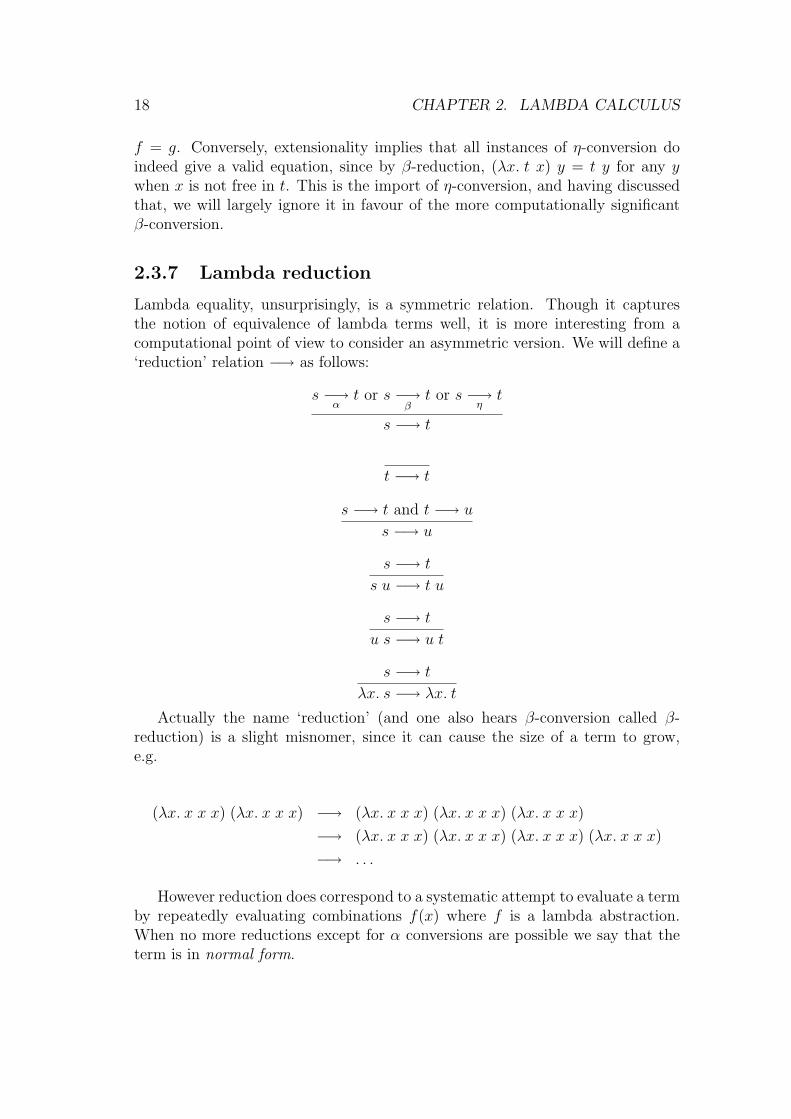
2.3.7 Lambda reduction
Lambda equality, unsurprisingly, is a symmetric relation. Though it capturesthe notion of equivalence of lambda terms well, it is more interesting from acomputational point of view to consider an asymmetric version. We will define a‘reduction’ relation −→ as follows:
s −→α
t or s −→β
t or s −→η
t
s −→ t
t −→ t
s −→ t and t −→ u
s −→ u
s −→ t
s u −→ t u
s −→ t
u s −→ u t
s −→ t
λx. s −→ λx. t
Actually the name ‘reduction’ (and one also hears β-conversion called β-reduction) is a slight misnomer, since it can cause the size of a term to grow,e.g.
(λx. x x x) (λx. x x x) −→ (λx. x x x) (λx. x x x) (λx. x x x)
−→ (λx. x x x) (λx. x x x) (λx. x x x) (λx. x x x)
−→ . . .
However reduction does correspond to a systematic attempt to evaluate a termby repeatedly evaluating combinations f(x) where f is a lambda abstraction.When no more reductions except for α conversions are possible we say that theterm is in normal form.
2.3. LAMBDA CALCULUS AS A FORMAL SYSTEM 19
2.3.8 Reduction strategies
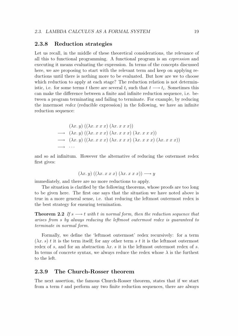
Let us recall, in the middle of these theoretical considerations, the relevance ofall this to functional programming. A functional program is an expression andexecuting it means evaluating the expression. In terms of the concepts discussedhere, we are proposing to start with the relevant term and keep on applying re-ductions until there is nothing more to be evaluated. But how are we to choosewhich reduction to apply at each stage? The reduction relation is not determin-istic, i.e. for some terms t there are several ti such that t −→ ti. Sometimes thiscan make the difference between a finite and infinite reduction sequence, i.e. be-tween a program terminating and failing to terminate. For example, by reducingthe innermost redex (reducible expression) in the following, we have an infinitereduction sequence:
(λx. y) ((λx. x x x) (λx. x x x))
−→ (λx. y) ((λx. x x x) (λx. x x x) (λx. x x x))
−→ (λx. y) ((λx. x x x) (λx. x x x) (λx. x x x) (λx. x x x))
−→ · · ·
and so ad infinitum. However the alternative of reducing the outermost redexfirst gives:
(λx. y) ((λx. x x x) (λx. x x x)) −→ y
immediately, and there are no more reductions to apply.The situation is clarified by the following theorems, whose proofs are too long
to be given here. The first one says that the situation we have noted above istrue in a more general sense, i.e. that reducing the leftmost outermost redex isthe best strategy for ensuring termination.
Theorem 2.2 If s −→ t with t in normal form, then the reduction sequence thatarises from s by always reducing the leftmost outermost redex is guaranteed toterminate in normal form.
Formally, we define the ‘leftmost outermost’ redex recursively: for a term(λx. s) t it is the term itself; for any other term s t it is the leftmost outermostredex of s, and for an abstraction λx. s it is the leftmost outermost redex of s.In terms of concrete syntax, we always reduce the redex whose λ is the furthestto the left.
2.3.9 The Church-Rosser theorem
The next assertion, the famous Church-Rosser theorem, states that if we startfrom a term t and perform any two finite reduction sequences, there are always

20 CHAPTER 2. LAMBDA CALCULUS
two more reduction sequences that bring the two back to the same term (thoughof course this might not be in normal form).
Theorem 2.3 If t −→ s1 and t −→ s2, then there is a term u such that s1 −→ uand s2 −→ u.
This has at least the following important consequences:
Corollary 2.4 If t1 = t2 then there is a term u with t1 −→ u and t2 −→ u.Proof: It is easy to see (by structural induction) that the equality relation = isin fact the symmetric transitive closure of the reduction relation. Now we canproceed by induction over the construction of the symmetric transitive closure.However less formally minded readers will probably find the following diagrammore convincing:
t1 t2@
@R�
�@
@R�
�@
@R�
�@
@R�
�@
@R�
�@
@R�
�@
@R�
�@
@R�
�@
@R�
�@
@R�
�u
We assume t1 = t2, so there is some sequence of reductions in both directions(i.e. the zigzag at the top) that connects them. Now the Church-Rosser theoremallows us to fill in the remainder of the sides in the above diagram, and hencereach the result by composing these reductions. Q.E.D.
Corollary 2.5 If t = t1 and t = t2 with t1 and t2 in normal form, then t1 ≡α t2,i.e. t1 and t2 are equal apart from α conversions.Proof: By the first corollary, we have some u with t1 −→ u and t2 −→ u. Butsince t1 and t2 are already in normal form, these reduction sequences to u canonly consist of alpha conversions. Q.E.D.
Hence normal forms, when they do exist, are unique up to alpha conversion.This gives us the first proof we have available that the relation of lambda equalityisn’t completely trivial, i.e. that there are any unequal terms. For example, sinceλx y. x and λx y. y are not interconvertible by alpha conversions alone, theycannot be equal.
Let us sum up the computational significance of all these assertions. In somesense, reducing the leftmost outermost redex is the best strategy, since it willwork if any strategy will. This is known as normal order reduction. On the otherhand any terminating reduction sequence will always give the same result, andmoreover it is never too late to abandon a given strategy and start using normalorder reduction. We will see later how this translates into practical terms.

2.4. COMBINATORS 21
2.4 Combinators
Combinators were actually developed as an independent theory by Schonfinkel(1924) before lambda notation came along. Moreover Curry rediscovered thetheory soon afterwards, independently of Schonfinkel and of Church. (When hefound out about Schonfinkel’s work, Curry attempted to contact him, but by thattime, Schonfinkel had been committed to a lunatic asylum.) We will distort thehistorical development by presenting the theory of combinators as an aspect oflambda calculus.
We will define a combinator simply to be a lambda term with no free vari-ables. Such a term is also said to be closed; it has a fixed meaning independentof the values of any variables. Now we will later, in the course of functionalprogramming, come across many useful combinators. But the cornerstone of thetheory of combinators is that one can get away with just a few combinators, andexpress in terms of those and variables any term at all: the operation of lambdaabstraction is unnecessary. In particular, a closed term can be expressed purelyin terms of these few combinators. We start by defining:
I = λx. x
K = λx y. x
S = λf g x. (f x)(g x)
We can motivate the names as follows.6 I is the identity function. K producesconstant functions:7 when applied to an argument a it gives the function λy. a.Finally S is a ‘sharing’ combinator, which takes two functions and an argumentand shares out the argument among the functions.8 Now we prove the following:
Lemma 2.6 For any lambda term t not involving lambda abstraction, there isa term u also not containing lambda abstractions, built up from S, K, I andvariables, with FV (u) = FV (t) − {x} and u = λx. t, i.e. u is lambda-equal toλx. t.Proof: By structural induction on the term t. By hypothesis, it cannot be anabstraction, so there are just three cases to consider.
• If t is a variable, then there are two possibilities. If it is equal to x, thenλx. x = I, so we are finished. If not, say t = y, then λx. y = K y.
• If t is a constant c, then λx. c = K c.
6We are not claiming these are the historical reasons for them.7Konstant — Schonfinkel was German, though in fact he originally used C.8One can imagine the argument x as some kind of environment of variables, making explicit
the state of an imperative language, so that in S f g x the functions f and g are evaluated inthe current state.
22 CHAPTER 2. LAMBDA CALCULUS
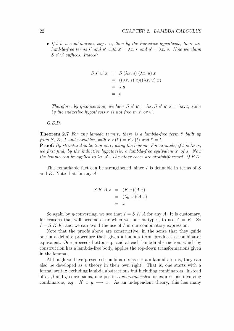
• If t is a combination, say s u, then by the inductive hypothesis, there arelambda-free terms s′ and u′ with s′ = λx. s and u′ = λx. u. Now we claimS s′ u′ suffices. Indeed:
S s′ u′ x = S (λx. s) (λx. u) x
= ((λx. s) x)((λx. u) x)
= s u
= t
Therefore, by η-conversion, we have S s′ u′ = λx. S s′ u′ x = λx. t, sinceby the inductive hypothesis x is not free in s′ or u′.
Q.E.D.
Theorem 2.7 For any lambda term t, there is a lambda-free term t′ built upfrom S, K, I and variables, with FV (t′) = FV (t) and t′ = t.Proof: By structural induction on t, using the lemma. For example, if t is λx. s,we first find, by the inductive hypothesis, a lambda-free equivalent s′ of s. Nowthe lemma can be applied to λx. s′. The other cases are straightforward. Q.E.D.
This remarkable fact can be strengthened, since I is definable in terms of Sand K. Note that for any A:
S K A x = (K x)(A x)
= (λy. x)(A x)
= x
So again by η-converting, we see that I = S K A for any A. It is customary,for reasons that will become clear when we look at types, to use A = K. SoI = S K K, and we can avoid the use of I in our combinatory expression.
Note that the proofs above are constructive, in the sense that they guideone in a definite procedure that, given a lambda term, produces a combinatorequivalent. One proceeds bottom-up, and at each lambda abstraction, which byconstruction has a lambda-free body, applies the top-down transformations givenin the lemma.
Although we have presented combinators as certain lambda terms, they canalso be developed as a theory in their own right. That is, one starts with aformal syntax excluding lambda abstractions but including combinators. Insteadof α, β and η conversions, one posits conversion rules for expressions involvingcombinators, e.g. K x y −→ x. As an independent theory, this has many

2.4. COMBINATORS 23
analogies with lambda calculus, e.g. the Church-Rosser theorem holds for thisnotion of reduction too. Moreover, the ugly difficulties connected with boundvariables are avoided completely. However the resulting system is, we feel, lessintuitive, since combinatory expressions can get rather obscure.
Apart from their purely logical interest, combinators have a certain practicalpotential. As we have already hinted, and as will become much clearer in the laterchapters, lambda calculus can be seen as a simple functional language, formingthe core of real practical languages like ML. We might say that the theorem ofcombinatory completeness shows that lambda calculus can be ‘compiled down’ toa ‘machine code’ of combinators. This computing terminology is not as fancifulas it appears. Combinators have been used as an implementation technique forfunctional languages, and real hardware has been built to evaluate combinatoryexpressions.
Further reading
An encyclopedic but clear book on lambda calculus is Barendregt (1984). Anotherpopular textbook is Hindley and Seldin (1986). Both these contain proofs of theresults that we have merely asserted. A more elementary treatment focusedtowards computer science is Part II of Gordon (1988). Much of our presentationhere and later is based on this last book.
Exercises
1. Find a normal form for (λx x x. x) a b c.
2. Define twice = λf x. f(fx). What is the intuitive meaning of twice?Find a normal form for twice twice twice f x. (Remember that functionapplication associates to the left.)
3. Find a term t such that t −→β
t. Is it true to say that a term is in normal
form if and only if whenever t −→ t′ then t ≡α t′?
4. What are the circumstances under which s[t/x][u/y] ≡α s[u/y][t/x]?
5. Find an equivalent in terms of the S, K and I combinators alone forλf x. f(x x).
6. Find a single combinator X such that all λ-terms are equal to a term builtfrom X and variables. You may find it helpful to consider A = λp.p K S Kand then think about A A A and A (A A).
7. Prove that any X is a fixed point combinator if and only if it is itself a fixedpoint of G, where G = λy m. m(y m).

Chapter 3
Lambda calculus as aprogramming language
One of the central questions studied by logicians in the 1930s was the Entschei-dungsproblem or ‘decision problem’. This asked whether there was some system-atic, mechanical procedure for deciding validity in first order logic. If it turnedout that there was, it would have fundamental philosophical, and perhaps practi-cal, significance. It would mean that a huge variety of complicated mathematicalproblems could in principle be solved purely by following some single fixed method— we would now say algorithm — no additional creativity would be required.
As it stands the question is hard to answer, because we need to define in math-ematical terms what it means for there to be a ‘systematic, mechanical’ procedurefor something. Perhaps Turing (1936) gave the best analysis, by arguing that themechanical procedures are those that could in principle be performed by a rea-sonably intelligent clerk with no knowledge of the underlying subject matter. Heabstracted from the behaviour of such a clerk and arrived at the famous notionof a ‘Turing machine’. Despite the fact that it arose by considering a human‘computer’, and was purely a mathematical abstraction, we now see a Turingmachine as a very simple computer. Despite being simple, a Turing machine iscapable of performing any calculation that can be done by a physical computer.1
A model of computation of equal power to a Turing machine is said to be Turingcomplete.
At about the same time, there were several other proposed definitions of‘mechanical procedure’. Most of these turned out to be equivalent in power toTuring machines. In particular, although it originally arose as a foundation formathematics, lambda calculus can also be seen as a programming language, to beexecuted by performing β-conversions. In fact, Church proposed before Turingthat the set of operations that can be expressed in lambda calculus formalizes the
1Actually more, since it neglects the necessary finite limit to the computer’s store. Arguablyany existing computer is actually a finite state machine, but the assumption of unboundedmemory seems a more fruitful abstraction.
24

25
intuitive idea of a mechanical procedure, a postulate known as Church’s thesis.Church (1936) showed that if this was accepted, the Entscheidungsproblem isunsolvable. Turing later showed that the functions definable in lambda calculusare precisely those computable by a Turing machine, which lent more credibilityto Church’s claims.
To a modern programmer, Turing machine programs are just about recog-nizable as a very primitive kind of machine code. Indeed, it seems that Turingmachines, and in particular Turing’s construction of a ‘universal machine’,2 werea key influence in the development of modern stored program computers, thoughthe extent and nature of this influence is still a matter for controversy (Robinson1994). It is remarkable that several of the other proposals for a definition of‘mechanical procedure’, often made before the advent of electronic computers,correspond closely to real programming methods. For example, Markov algo-rithms, the standard approach to computability in the (former) Soviet Union,can be seen as underlying the programming language SNOBOL. In what follows,we are concerned with the influence of lambda calculus on functional program-ming languages.
LISP, the second oldest high level language (FORTRAN being the oldest)took a few ideas from lambda calculus, in particular the notation ‘(LAMBDA · · ·)’for anonymous functions. However it was not really based on lambda calculusat all. In fact the early versions, and some current dialects, use a system ofdynamic binding that does not correspond to lambda calculus. (We will discussthis later.) Moreover there was no real support for higher order functions, whilethere was considerable use of imperative features. Nevertheless LISP deserves tobe considered as the first functional programming language, and pioneered manyof the associated techniques such as automatic storage allocation and garbagecollection.
The influence of lambda calculus really took off with the work of Landin andStrachey in the 60s. In particular, Landin showed how many features of current(imperative) languages could usefully be analyzed in terms of lambda calculus,e.g. the notion of variable scoping in Algol 60. Landin (1966) went on to proposethe use of lambda calculus as a core for programming languages, and inventeda functional language ISWIM (‘If you See What I Mean’). This was widelyinfluential and spawned many real languages.
ML started life as the metalanguage (hence the name ML) of a theorem prov-ing system called Edinburgh LCF (Gordon, Milner, and Wadsworth 1979). Thatis, it was intended as a language in which to write algorithms for proving theo-rems in a formal deductive calculus. It was strongly influenced by ISWIM butadded an innovative polymorphic type system including abstract types, as well asa system of exceptions to deal with error conditions. These facilities were dictated
2A single Turing machine program capable of simulating any other — we would now regardit as an interpreter. You will learn about this in the course on Computation Theory.

26CHAPTER 3. LAMBDA CALCULUS AS A PROGRAMMING LANGUAGE
by the application at hand, and this policy resulted in a coherent and focuseddesign. This narrowness of focus is typical of successful languages (C is anothergood example) and contrasts sharply with the failure of committee-designed lan-guages like Algol 60 which have served more as a source of important ideas thanas popular practical tools. We will have more to say about ML later. Let us nowsee how pure lambda calculus can be used as a programming language.
3.1 Representing data in lambda calculus
Programs need data to work on, so we start by fixing lambda expressions toencode data. Furthermore, we define a few basic operations on this data. In manycases, we show how a string of human-readable syntax s can be translated directlyinto a lambda expression s′. This procedure is known as ‘syntactic sugaring’ —it makes the bitter pill of pure lambda notation easier to digest. We write suchdefinitions as:
s4= s′
This notation means ‘s = s′ by definition’; one also commonly sees this writtenas ‘s =def s′’. If preferred, we could always regard these as defining a singleconstant denoting that operation, which is then applied to arguments in the usuallambda calculus style, the surface notation being irrelevant. For example we canimagine ‘if E then E1 else E2’ as ‘COND E E1 E2’ for some constant COND. Insuch cases, any variables on the left of the definition need to be abstracted over,e.g. instead of
fst p4= p true
(see below) we could write
fst4= λp. p true
3.1.1 Truth values and the conditional
We can use any unequal lambda expressions to stand for ‘true’ and ‘false’, butthe following work particularly smoothly:
true4= λx y. x
false4= λx y. y
Given those definitions, we can easily define a conditional expression just likeC’s ‘?:’ construct. Note that this is a conditional expression not a conditional
3.1. REPRESENTING DATA IN LAMBDA CALCULUS 27
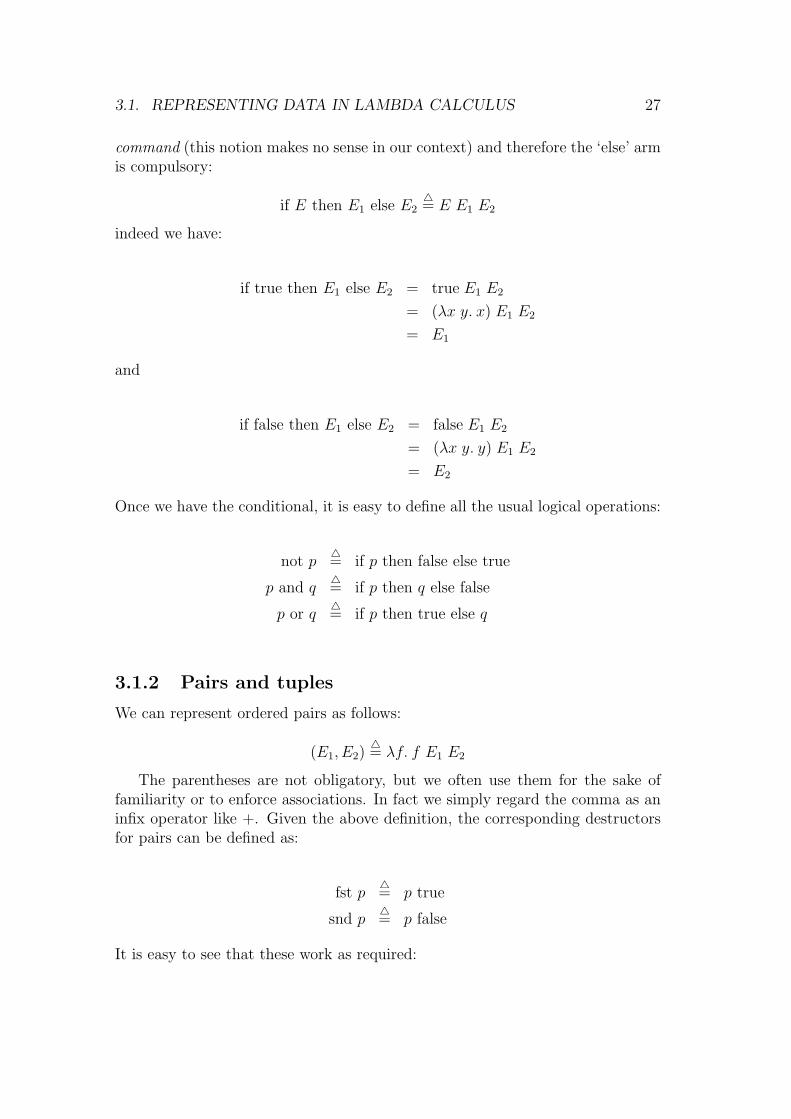
command (this notion makes no sense in our context) and therefore the ‘else’ armis compulsory:
if E then E1 else E24= E E1 E2
indeed we have:
if true then E1 else E2 = true E1 E2
= (λx y. x) E1 E2
= E1
and
if false then E1 else E2 = false E1 E2
= (λx y. y) E1 E2
= E2
Once we have the conditional, it is easy to define all the usual logical operations:
not p4= if p then false else true
p and q4= if p then q else false
p or q4= if p then true else q
3.1.2 Pairs and tuples
We can represent ordered pairs as follows:
(E1, E2)4= λf. f E1 E2
The parentheses are not obligatory, but we often use them for the sake offamiliarity or to enforce associations. In fact we simply regard the comma as aninfix operator like +. Given the above definition, the corresponding destructorsfor pairs can be defined as:
fst p4= p true
snd p4= p false
It is easy to see that these work as required:

28CHAPTER 3. LAMBDA CALCULUS AS A PROGRAMMING LANGUAGE
fst (p, q) = (p, q) true
= (λf. f p q) true
= true p q
= (λx y. x) p q
= p
and
snd (p, q) = (p, q) false
= (λf. f p q) false
= false p q
= (λx y. y) p q
= q
We can build up triples, quadruples, quintuples, indeed arbitrary n-tuples, byiterating the pairing construct:
(E1, E2, . . . , En) = (E1, (E2, . . . En))
We need simply say that the infix comma operator is right-associative, andcan understand this without any other conventions. For example:
(p, q, r, s) = (p, (q, (r, s)))
= λf. f p (q, (r, s))
= λf. f p (λf. f q (r, s))
= λf. f p (λf. f q (λf. f r s))
= λf. f p (λg. g q (λh. h r s))
where in the last line we have performed an alpha-conversion for the sake ofclarity. Although tuples are built up in a flat manner, it is easy to create arbitraryfinitely-branching tree structures by using tupling repeatedly. Finally, if oneprefers conventional functions over Cartesian products to our ‘curried’ functions,one can convert between the two using the following:
CURRY f4= λx y. f(x, y)
UNCURRY g4= λp. g (fst p) (snd p)

3.1. REPRESENTING DATA IN LAMBDA CALCULUS 29
These special operations for pairs can easily be generalized to arbitrary n-tuples. For example, we can define a selector function to get the ith componentof a flat tuple p. We will write this operation as (p)i and define (p)1 = fst pand the others by (p)i = fst (sndi−1 p). Likewise we can generalize CURRY andUNCURRY:
CURRYn f4= λx1 · · · xn. f(x1, . . . , xn)
UNCURRYn g4= λp. g (p)1 · · · (p)n
We can now write λ(x1, . . . , xn). t as an abbreviation for:
UNCURRYn (λx1 · · · xn. t)
giving a natural notation for functions over Cartesian products.
3.1.3 The natural numbers
We will represent each natural number n as follows:3
n4= λf x. fn x
that is, 0 = λf x. x, 1 = λf x. f x, 2 = λf x. f (f x) etc. These representa-tions are known as Church numerals, though the basic idea was used earlier byWittgenstein (1922).4 They are not a very efficient representation, amountingessentially to counting in unary, 1, 11, 111, 1111, 11111, 111111, . . .. There are,from an efficiency point of view, much better ways of representing numbers, e.g.tuples of trues and falses as binary expansions. But at the moment we are onlyinterested in computability ‘in principle’ and Church numerals have various niceformal properties. For example, it is easy to give lambda expressions for thecommon arithmetic operators such as the successor operator which adds one toits argument:
SUC4= λn f x. n f (f x)
Indeed
SUC n = (λn f x. n f (f x))(λf x. fn x)
= λf x. (λf x. fn x)f (f x)
= λf x. (λx. fn x)(f x)
3The n in fn x is just a meta-notation, and does not mean that there is anything circularabout our definition.
4‘6.021 A number is the exponent of an operation’.

30CHAPTER 3. LAMBDA CALCULUS AS A PROGRAMMING LANGUAGE
= λf x. fn (f x)
= λf x. fn+1 x
= n + 1
Similarly it is easy to test a numeral to see if it is zero:
ISZERO n4= n (λx. false) true
since:
ISZERO 0 = (λf x. x)(λx. false) true = true
and
ISZERO (n + 1) = (λf x. fn+1x)(λx. false)true
= (λx. false)n+1 true
= (λx. false)((λx. false)n true)
= false
The following perform addition and multiplication on Church numerals:
m + n4= λf x. m f (n f x)
m ∗ n4= λf x. m (n f) x
Indeed:
m + n = λf x. m f (n f x)
= λf x. (λf x. fm x) f (n f x)
= λf x. (λx. fm x) (n f x)
= λf x. fm (n f x)
= λf x. fm ((λf x. fn x) f x)
= λf x. fm ((λx. fn x) x)
= λf x. fm (fn x)
= λf x. fm+nx
and:
m ∗ n = λf x. m (n f) x
= λf x. (λf x. fm x) (n f) x
3.2. RECURSIVE FUNCTIONS 31
= λf x. (λx. (n f)m x) x
= λf x. (n f)m x
= λf x. ((λf x. fn x) f)m x
= λf x. ((λx. fn x)m x
= λf x. (fn)m x
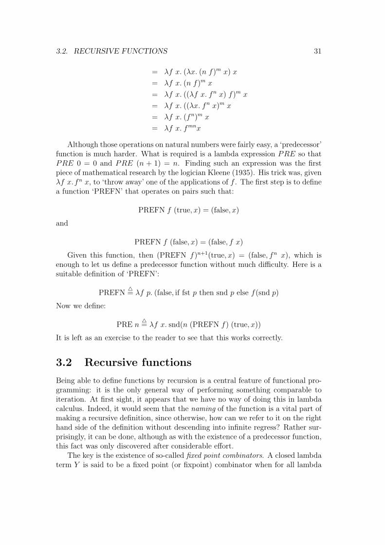
= λf x. fmnx
Although those operations on natural numbers were fairly easy, a ‘predecessor’function is much harder. What is required is a lambda expression PRE so thatPRE 0 = 0 and PRE (n + 1) = n. Finding such an expression was the firstpiece of mathematical research by the logician Kleene (1935). His trick was, givenλf x.fn x, to ‘throw away’ one of the applications of f . The first step is to definea function ‘PREFN’ that operates on pairs such that:
PREFN f (true, x) = (false, x)
and
PREFN f (false, x) = (false, f x)
Given this function, then (PREFN f)n+1(true, x) = (false, fn x), which isenough to let us define a predecessor function without much difficulty. Here is asuitable definition of ‘PREFN’:
PREFN4= λf p. (false, if fst p then snd p else f(snd p)
Now we define:
PRE n4= λf x. snd(n (PREFN f) (true, x))
It is left as an exercise to the reader to see that this works correctly.
3.2 Recursive functions
Being able to define functions by recursion is a central feature of functional pro-gramming: it is the only general way of performing something comparable toiteration. At first sight, it appears that we have no way of doing this in lambdacalculus. Indeed, it would seem that the naming of the function is a vital part ofmaking a recursive definition, since otherwise, how can we refer to it on the righthand side of the definition without descending into infinite regress? Rather sur-prisingly, it can be done, although as with the existence of a predecessor function,this fact was only discovered after considerable effort.
The key is the existence of so-called fixed point combinators. A closed lambdaterm Y is said to be a fixed point (or fixpoint) combinator when for all lambda

32CHAPTER 3. LAMBDA CALCULUS AS A PROGRAMMING LANGUAGE
terms f , we have f(Y f) = Y f . That is, a fixed point combinator, given anyterm f as an argument, returns a fixed point for f , i.e. a term x such thatf(x) = x. The first such combinator to be found (by Curry) is usually called Y .It can be motivated by recalling the Russell paradox, and for this reason is oftencalled the ‘paradoxical combinator’. We defined:
R = λx. ¬(x x)
and found that:
R R = ¬(R R)
That is, R R is a fixed point of the negation operator. So in order to get ageneral fixed point combinator, all we need to do is generalize ¬ into whateverfunction is given it as argument. Therefore we set:
Y4= λf. (λx. f(x x))(λx. f(x x))
It is a simple matter to show that it works:
Y f = (λf. (λx. f(x x))(λx. f(x x))) f
= (λx. f(x x))(λx. f(x x))
= f((λx. f(x x))(λx. f(x x)))
= f(Y f)
Though valid from a mathematical point of view, this is not so attractive froma programming point of view since the above was only valid for lambda equality,not reduction (in the last line we performed a backwards beta conversion). Forthis reason the following alternative, due to Turing, may be preferred:
T4= (λx y. y (x x y)) (λx y. y (x x y))
(The proof that T f −→ f(T f) is left as an exercise.) However it doesno harm if we simply allow Y f to be beta-reduced throughout the reductionsequence for a recursively defined function. Now let us see how to use a fixedpoint combinator (say Y ) to implement recursive functions. We will take thefactorial function as an example. We want to define a function fact with:
fact(n) = if ISZERO n then 1 else n ∗ fact(PRE n)
The first step is to transform this into the following equivalent:
fact = λn. if ISZERO n then 1 else n ∗ fact(PRE n)
which in its turn is equivalent to:

3.3. LET EXPRESSIONS 33
fact = (λf n. if ISZERO n then 1 else n ∗ f(PRE n)) fact
This exhibits fact as the fixed point of a function F , namely:
F = λf n. if ISZERO n then 1 else n ∗ f(PRE n)
Consequently we merely need to set fact = Y F . Similar techniques work formutually recursive functions, i.e. a set of functions whose definitions are mutuallydependent. A definition such as:
f1 = F1 f1 · · · fn
f2 = F2 f1 · · · fn
. . . = . . .
fn = Fn f1 · · · fn
can be transformed, using tuples, into a single equation:
(f1, f2, . . . , fn) = (F1 f1 · · · fn, F2 f1 · · · fn, . . . , Fn f1 · · · fn)
If we now write t = (f1, f2, . . . , fn), then each of the functions on the right canbe recovered by applying the appropriate selector to t: we have fi = (t)i. Afterabstracting out t, this gives an equation in the canonical form t = F t which canbe solved by t = Y F . Now the individual functions can be recovered from t bythe same method of selecting components of the tuple.
3.3 Let expressions
We’ve touted the ability to write anonymous functions as one of the merits oflambda calculus, and shown that names are not necessary to define recursivefunctions. Nevertheless it is often useful to be able to give names to expressions,to avoid tedious repetition of large terms. A simple form of naming can besupported as another syntactic sugar on top of pure lambda calculus:
let x = s in t4= (λx. t) s
For example, as we would expect:
(let z = 2 + 3 in z + z) = (λz. z + z) (2 + 3) = (2 + 3) + (2 + 3)
We can achieve the binding of multiple names to expressions either in a serialor parallel fashion. For the first, we will simply iterate the above construct. Forthe latter, we will write multiple bindings separated by ‘and’:

34CHAPTER 3. LAMBDA CALCULUS AS A PROGRAMMING LANGUAGE
let x1 = s1 and · · · and xn = sn in t
and regard it as syntactic sugar for:
(λ(x1, . . . , xn). t) (s1, . . . , sn)
To illustrate the distinction between serial and parallel binding, consider:
let x = 1 in let x = 2 in let y = x in x + y
which should yield 4, while:
let x = 1 in let x = 2 and y = x in x + y
should yield 3. We will also allow arguments to names bound by ‘let’; againthis can be regarded as syntactic sugar, with f x1 · · · xn = t meaning f =λx1 · · · xn. t. Instead of a prefix ‘let x = s in t’, we will allow a postfix version,which is sometimes more readable:
t where x = s
For example, we might write ‘y < y2 where y = 1 + x’. Normally, the ‘let’and ‘where’ constructs will be interpreted as above, in a non-recursive fashion.For example:
let x = x− 1 in · · ·
binds x to one less than whatever value it is bound to outside, rather than tryingto bind x to the fixed point of x = x−1.5 However where a recursive interpretationis required, we add the word ‘rec’, writing ‘let rec’ or ‘where rec’, e.g.
let rec fact(n) = if ISZERO n then 1 else n ∗ fact(PRE n)
This can be regarded as a shorthand for ‘let fact = Y F ’ where
F = λf n. if ISZERO n then 1 else n ∗ f(PRE n)
as explained above.
5There is such a fixed point, but the lambda term involved has no normal form, so is in asense ‘undefined’. The semantics of nonterminating terms is subtle, and we will not considerit at length here. Actually, the salient question is not whether a term has a normal formbut whether it has a so-called head normal form — see Barendregt (1984) and also Abramsky(1990).

3.4. STEPS TOWARDS A REAL PROGRAMMING LANGUAGE 35
3.4 Steps towards a real programming language
We have established a fairly extensive system of ‘syntactic sugar’ to support ahuman-readable syntax on top of pure lambda calculus. It is remarkable thatthis device is enough to bring us to the point where we can write the definitionof the factorial function almost in the way we can in ML. In what sense, though,is the lambda calculus augmented with these notational conventions really aprogramming language?
Ultimately, a program is just a single expression. However, given the use oflet to bind various important subexpressions to names, it is natural instead toview the program as a set of definitions of auxiliary functions, followed finally bythe expression itself, e.g:
let rec fact(n) = if ISZERO n then 1 else n ∗ fact(PRE n) in· · ·fact(6)
We can read these definitions of auxiliary functions as equations in the mathe-matical sense. Understood in this way, they do not give any explicit instructionson how to evaluate expressions, or even in which direction the equations areto be used. For this reason, functional programming is often referred to as adeclarative programming method, as also is logic programming (e.g. PROLOG).6
The program does not incorporate explicit instructions, merely declares certainproperties of the relevant notions, and leaves the rest to the machine.
At the same time, the program is useless, or at least ambiguous, unless themachine somehow reacts sensibly to it. Therefore it must be understood thatthe program, albeit from a superficial point of view purely declarative, is to beexecuted in a certain way. In fact, the expression is evaluated by expandingall instances of defined notions (i.e. reading the equations from left to right),and then repeatedly performing β-conversions. That is, although there seems tobe no procedural information in the program, a particular execution strategy isunderstood. In a sense then, the term ‘declarative’ is largely a matter of humanpsychology.
Moreover, there must be a definite convention for the reduction strategy touse, for we know that different choices of β-redex can lead to different behaviourwith respect to termination. Consequently, it is only when we specify this thatwe really get a definite programming language. We will see in later chapters howdifferent functional languages make different choices here. But first we pause toconsider the incorporation of types.
6Apparently Landin preferred ‘denotative’ to ‘declarative’.

36CHAPTER 3. LAMBDA CALCULUS AS A PROGRAMMING LANGUAGE
3.5 Further reading
Many of the standard texts already cited include details about the matters dis-cussed here. In particular Gordon (1988) gives a clear proof that lambda calculusis Turing-complete, and that the lambda calculus analog of the ‘halting problem’(whether a term has a normal form) is unsolvable. The influence of lambda cal-culus on real programming languages and the evolution of functional languagesare discussed by Hudak (1989).
Exercises
1. Justify ‘generalized β-conversion’, i.e. prove that:
(λ(x1, . . . , xn). t[x1, . . . , xn])(t1, . . . , tn) = t[t1, . . . , tn]
2. Define f ◦ g4= λx. f(g x), and recall that I = λx. x. Prove that CURRY ◦
UNCURRY = I. Is it also true that UNCURRY ◦ CURRY = I?.
3. What arithmetical operation does λn f x. f(n f x) perform on Churchnumerals? What about λm n. n m?
4. Prove that the following (due to Klop) is a fixed point combinator:
££££££££££££££££££££££££££
where:
£4= λabcdefghijklmnopqstuvwxyzr. r(thisisafixedpointcombinator)
5. Make a recursive definition of natural number subtraction.
6. Consider the following representation of lists, due to Mairson (1991):
nil = λc n. n
cons = λx l c n. c x (l c n)
head = λl. l(λx y. x) nil
tail = λl. snd (l(λx p. (cons x (fst p), fst p)) (nil, nil))
append = λl1 l2. l1 cons l2
append lists = λL. L append nil
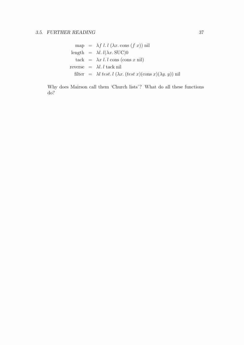
3.5. FURTHER READING 37
map = λf l. l (λx. cons (f x)) nil
length = λl. l(λx. SUC)0
tack = λx l. l cons (cons x nil)
reverse = λl. l tack nil
filter = λl test. l (λx. (test x)(cons x)(λy. y)) nil
Why does Mairson call them ‘Church lists’? What do all these functionsdo?
Chapter 4
Types
Types are a means of distinguishing different sorts of data, like booleans, naturalnumbers and functions, and making sure that these distinctions are respected,by, for example, ensuring that functions cannot be applied to arguments of thewrong type. Why should we want to add types to lambda calculus, and toprogramming languages derived from it? We can distinguish reasons from logicand reasons from programming.
From the logical point of view, we have seen that the Russell paradox makesit difficult to extend lambda calculus with set theory without contradiction. TheRussell paradox may well arise because of the peculiar self-referential nature ofthe trick involved: we apply a function to itself. Even if it weren’t necessary toavoid paradox, we might feel that intuitively we really have a poor grip of what’sgoing on in a system where we can do such things. Certainly applying somefunctions to themselves, e.g. the identity function λx. x or a constant functionλx. y, seems quite innocuous. But surely we would have a clearer picture of whatsort of functions lambda terms denote if we knew exactly what their domains andcodomains were, and only applied them to arguments in their domains. Thesewere the sorts of reasons why Russell originally introduced types in PrincipiaMathematica.
Types also arose, perhaps at first largely independently of the above con-siderations, in programming languages, and since we view lambda calculus as aprogramming language, this motivates us too. Even FORTRAN distinguishedintegers and floating point values. One reason was clearly efficiency: the machinecan generate more efficient code, and use storage more effectively, by knowingmore about a variable. For example the implementation of C’s pointer arith-metic varies according to the size of the referenced objects. If p is a pointer toobjects occupying 4 bytes, then what C programmers write as p+1 becomes p+4inside a byte-addressed machine. C’s ancestor BCPL is untyped, and is thereforeunable to distinguish pointers from integers; to support the same style of pointerarithmetic it is necessary to apply a scaling at every indirection, a significantpenalty.
38
4.1. TYPED LAMBDA CALCULUS 39
Apart from efficiency, as time went by, types also began to be appreciatedmore and more for their value in providing limited static checks on programs.Many programming errors, either trivial typos or more substantial conceptualerrors, are suggested by type clashes, and these can be detected before running theprogram, during the compilation process. Moreover, types often serve as usefuldocumentation for people reading code. Finally, types can be used to achievebetter modularization and data hiding by ‘artificially’ distinguishing some datastructure from its internal representation.
At the same time, some programmers dislike types, because they find therestrictions placed on their programming style irksome. There are untyped pro-gramming languages, imperative ones like BCPL and functional ones like ISWIM,SASL and Erlang. Others, like PL/I, have only weak typing, with the compilerallowing some mixtures of different types and casting them appropriately. Thereare also languages like LISP that perform typechecking dynamically, during exe-cution, rather than statically during compilation. This can (at least in principle)degrade runtime performance, since it means that the computer is spending sometime on making sure types are respected during execution — compare checking ofarray bounds during execution, another common runtime overhead. By contrast,we have suggested that static typing, if anything, can improve performance.
Just how restrictive a type system is found depends a lot on the nature of theprogrammer’s applications and programming style. Finding a type system thatallows useful static typechecking, while at the same time allowing programmersplenty of flexibility, is still an active research area. The ML type system is animportant step along this road, since it features polymorphism, allowing the samefunction to be used with various different types. This retains strong static type-checking while giving some of the benefits of weak or dynamic typing.1 Moreover,programmers never need to specify any types in ML — the computer can infera most general type for every expression, and reject expressions that are not ty-pable. We will consider polymorphism in the setting of lambda calculus below.Certainly, the ML type system provides a congenial environment for many kindsof programming. Nevertheless, we do not want to give the impression that it isnecessarily the answer to all programming problems.
4.1 Typed lambda calculus
It is a fairly straightforward matter to modify lambda calculus with a notion oftype, but the resulting changes, as we shall see, are far-reaching. The basic ideais that every lambda term has a type, and a term s can only be applied to a termt in a combination s t when the types match up appropriately, i.e. s has the typeof a function σ → τ and t has type σ. The result, s t, then has type τ . This is,in programming language parlance, strong typing. The term t must have exactly
1As well, perhaps, as some of the overheads.
40 CHAPTER 4. TYPES
the type σ; there is no notion of subtyping or coercion. This contrasts with someprogramming languages like C where a function expecting an argument of typefloat or double will accept one of type int and appropriately cast it. Similarnotions of subtyping and coercion can also be added to lambda calculus, but toconsider these here would lead us too far astray.
We will use ‘t : σ’ to mean ‘t has type σ’. This is already the standard notationin mathematics where function spaces are concerned, because f : σ → τ meansthat f is a function from the set σ to the set τ . We will think of types as sets inwhich the corresponding objects live, and imagine t : σ to mean t ∈ σ. Thoughthe reader may like to do likewise, as a heuristic device, we will view typed lambdacalculus purely as a formal system and make the rules independent of any suchinterpretation.
4.1.1 The stock of types
The first stage in our formalization is to specify exactly what the types are.We suppose first of all that we have some set of primitive types, which might,for example, contain bool and int. We can construct composite types fromthese using the function space type constructor. Formally, we make the followinginductive definition of the set TyC of types based on a set of primitive types C:
σ ∈ C
σ ∈ TyC
σ ∈ TyC τ ∈ TyC
σ → τ ∈ TyC
For example, possible types might be int, bool → bool and (int → bool) →int → bool. We assume that the function arrow associates to the right, i.e.σ → τ → υ means σ → (τ → υ). This fits naturally with the other syntacticconventions connected with currying.
Before long, we shall extend the type system in two ways. First, we willallow so-called type variables as well as primitive type constants — these are thevehicle for polymorphism. Secondly, we will allow the introduction of other typeconstructors besides the function arrow. For example, we will later introduce aconstructor × for the product type. In that case a new clause:
σ ∈ TyC τ ∈ TyC
σ × τ ∈ TyC
needs to be added to the inductive definition. Once we move to the more concretecase of ML, there is the possibility of new, user-defined types and type construc-tors, so we will get used to arbitrary sets of constructors of any arity. We willwrite (α1, . . . , αn)con for the application of an n-ary type constructor con to thearguments αi. (Only in a few special cases like → and × do we use infix syntax,

4.1. TYPED LAMBDA CALCULUS 41
for the sake of familiarity.) For example (σ)list is the type of lists whose elementsall have type σ.
An important property of the types, provable because of free inductive gen-eration, is that σ → τ 6= σ. (In fact, more generally, a type cannot be the sameas any proper syntactic subexpression of itself.) This rules out the possibility ofapplying a term to itself, unless the two instances in question have distinct types.
4.1.2 Church and Curry typing
There are two major approaches to defining typed lambda calculus. One ap-proach, due to Church, is explicit. A (single) type is attached to each term.That is, in the construction of terms, the untyped terms that we have presentedare modified with an additional field for the type. In the case of constants, thistype is pre-assigned, but variables may be of any type. The rules for valid termformation are then:
v : σ
Constant c has type σ
c : σ
s : σ → τ t : σ
s t : τ
v : σ t : τ
λv. t : σ → τ
For our purposes, however, we prefer Curry’s approach to typing, which ispurely implicit. The terms are exactly as in the untyped case, and a term mayor may not have a type, and if it does, may have many different types.2 Forexample, the identity function λx. x may be given any type of the form σ → σ,reasonably enough. There are two related reasons why we prefer this approach.First, it provides a smoother treatment of ML’s polymorphism, and secondly, itcorresponds well to the actual use of ML, where it is never necessary to specifytypes explicitly.
At the same time, some of the formal details of Curry-style type assignmentare a bit more complex. We do not merely define a relation of typability inisolation, but with respect to a context, i.e. a finite set of typing assumptionsabout variables. We write:
Γ ` t : σ
2Some purists would argue that this isn’t properly speaking ‘typed lambda calculus’ butrather ‘untyped lambda calculus with a separate notion of type assignment’.

42 CHAPTER 4. TYPES
to mean ‘in context Γ, the term t can be given type σ’. (We will, however, write` t : σ or just t : σ when the typing judgement holds in the empty context.) Theelements of Γ are of the form v : σ, i.e. they are themselves typing assumptionsabout variables, typically those that are components of the term. We assumethat Γ never gives contradictory assignments to the same variable; if preferredwe can think of it as a partial function from the indexing set of the variablesinto the set of types. The use of the symbol ` corresponds to its general use forjudgements in logic of the form Γ ` φ, read as ‘φ follows from assumptions Γ’.
4.1.3 Formal typability rules
The rules for typing expressions are fairly natural. Remember the interpretationof t : σ as ‘t could be given type σ’.
v : σ ∈ Γ
Γ ` v : σ
Constant c has type σ
c : σ
Γ ` s : σ → τ Γ ` t : σ
Γ ` s t : τ
Γ ∪ {v : σ} ` t : τ
Γ ` λv. t : σ → τ
Once again, this is to be regarded as an inductive definition of the typabilityrelation, so a term only has a type if it can be derived by the above rules. Forexample, let us see how to type the identity function. By the rule for variableswe have:
{x : σ} ` x : σ
and therefore by the last rule we get:
∅ ` λx. x : σ → σ
By our established convention for empty contexts, we write simply λx. x :σ → σ. This example also illustrates the need for the context in Curry typing,and why it can be avoided in the Church version. Without the context we coulddeduce x : τ for any τ , and then by the last rule get λx. x : σ → τ , clearly atvariance with the intuitive interpretation of the identity function. This problemdoesn’t arise in Church typing, since in that case either both variables have typeσ, in which case the rules imply that λx.x : σ → σ, or else the two x’s are actuallydifferent variables, since their types differ and the types are a component of theterm. Now, indeed, λx : σ. (x : τ) : σ → τ , but this is reasonable because the
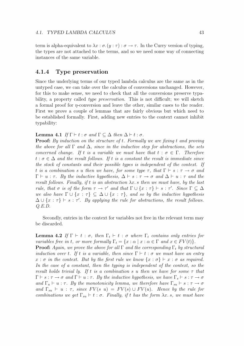
4.1. TYPED LAMBDA CALCULUS 43
term is alpha-equivalent to λx : σ. (y : τ) : σ → τ . In the Curry version of typing,the types are not attached to the terms, and so we need some way of connectinginstances of the same variable.
4.1.4 Type preservation
Since the underlying terms of our typed lambda calculus are the same as in theuntyped case, we can take over the calculus of conversions unchanged. However,for this to make sense, we need to check that all the conversions preserve typa-bility, a property called type preservation. This is not difficult; we will sketcha formal proof for η-conversion and leave the other, similar cases to the reader.First we prove a couple of lemmas that are fairly obvious but which need tobe established formally. First, adding new entries to the context cannot inhibittypability:
Lemma 4.1 If Γ ` t : σ and Γ ⊆ ∆ then ∆ ` t : σ.Proof: By induction on the structure of t. Formally we are fixing t and provingthe above for all Γ and ∆, since in the inductive step for abstractions, the setsconcerned change. If t is a variable we must have that t : σ ∈ Γ. Thereforet : σ ∈ ∆ and the result follows. If t is a constant the result is immediate sincethe stock of constants and their possible types is independent of the context. Ift is a combination s u then we have, for some type τ , that Γ ` s : τ → σ andΓ ` u : τ . By the inductive hypothesis, ∆ ` s : τ → σ and ∆ ` u : τ and theresult follows. Finally, if t is an abstraction λx. s then we must have, by the lastrule, that σ is of the form τ → τ ′ and that Γ ∪ {x : τ} ` s : τ ′. Since Γ ⊆ ∆we also have Γ ∪ {x : τ} ⊆ ∆ ∪ {x : τ}, and so by the inductive hypothesis∆ ∪ {x : τ} ` s : τ ′. By applying the rule for abstractions, the result follows.Q.E.D.
Secondly, entries in the context for variables not free in the relevant term maybe discarded.
Lemma 4.2 If Γ ` t : σ, then Γt ` t : σ where Γt contains only entries forvariables free in t, or more formally Γt = {x : α | x : α ∈ Γ and x ∈ FV (t)}.Proof: Again, we prove the above for all Γ and the corresponding Γt by structuralinduction over t. If t is a variable, then since Γ ` t : σ we must have an entryx : σ in the context. But by the first rule we know {x : σ} ` x : σ as required.In the case of a constant, then the typing is independent of the context, so theresult holds trivial ly. If t is a combination s u then we have for some τ thatΓ ` s : τ → σ and Γ ` u : τ . By the inductive hypothesis, we have Γs ` s : τ → σand Γu ` u : τ . By the monotonicity lemma, we therefore have Γsu ` s : τ → σand Γsu ` u : τ , since FV (s u) = FV (s) ∪ FV (u). Hence by the rule forcombinations we get Γsu ` t : σ. Finally, if t has the form λx. s, we must have

44 CHAPTER 4. TYPES
Γ ∪ {x : τ} ` s : τ ′ with σ of the form τ → τ ′. By the inductive hypothesis wehave (Γ ∪ {x : τ})s ` s : τ ′, and so (Γ ∪ {x : τ})s − {x : τ} ` (λx. s) : σ. Now weneed simply observe that (Γ ∪ {x : τ})s − {x : τ} ⊆ Γt and appeal once more tomonotonicity. Q.E.D.
Now we come to the main result.
Theorem 4.3 If Γ ` t : σ and t −→η
t′, then also Γ ` t′ : σ
Proof: Since by hypothesis t is an η-redex, it must be of the form (λx.t x) with x 6∈FV (t). Now, its type can only have arisen by the last typing rule, and thereforeσ must be of the form τ → τ ′, and we must have {x : τ} ` (t x) : τ ′. Now, thistyping can only have arisen by the rule for combinations. Since the context canonly give one typing to each variable, we must therefore have {x : τ} ` t : τ → τ ′.But since by hypothesis, x 6∈ FV (t), the lemma yields ` t : τ → τ ′ as required.Q.E.D.
Putting together all these results for other conversions, we see that if Γ ` t : σand t −→ t′, then we have Γ ` t′ : σ. This is reassuring, since if the evaluationrules that are applied during execution could change the types of expressions, itwould cast doubt on the whole enterprise of static typing.
4.2 Polymorphism
The Curry typing system already gives us a form of polymorphism, in that agiven term may have different types. Let us start by distinguish between thesimilar concepts of polymorphism and overloading. Both of them mean that anexpression may have multiple types. However in the case of polymorphism, allthe types bear a systematic relationship to each other, and all types following thepattern are allowed. For example, the identity function may have type σ → σ,or τ → τ , or (σ → τ) → (σ → τ), but all the instances have the same structure.By contrast, in overloading, a given function may have different types that bearno structural relation to each other, or only certain instances may be selected.For example, a function + may be allowed to have type int → int → int or typefloat → float → float, but not bool → bool → bool.3 Yet a third related notionis subtyping, which is a more principled version of overloading, regarding certaintypes as embedded in others. This, however, turns out to be a lot more complexthan it seems.4
3Strachey, who coined the term ‘polymorphism’, referred to what we call polymorphism andoverloading as parametric and ad hoc polymorphism respectively.
4For example, if α is a subtype of α′, should α → β be a subtype or a supertype of α′ → β?One can defend either interpretation (‘covariant’ or ‘contravariant’) in certain situations.

4.2. POLYMORPHISM 45
4.2.1 Let polymorphism
Unfortunately the type system we have so far places some unpleasant restrictionson polymorphism. For example, the following expression is perfectly acceptable:
if (λx. x) true then (λx. x) 1 else 0
Here is a proof according to the above rules. We assume that the constantscan be typed in the empty environment, and we fold together two successiveapplications of the rule for combinations as a rule for if, remembering that‘if b then t1 else t2’ is shorthand for ‘COND b t1 t2’.
{x : bool} ` x : bool
` (λx. x) : bool → bool ` true : bool
` (λx. x) true : bool
{x : int} ` x : int
` (λx. x) : int → int ` 1 : int
` (λx. x) 1 : int ` 0 : int
` if (λx. x) true then (λx. x) 1 else 0 : int
The two instances of the identity function get types bool → bool and int → int.But consider the following:
let I = λx. x in if I true then I 1 else 0
According to our definitions, this is just syntactic sugar for:
(λI. if I true then I 1 else 0) (λx. x)
As the reader may readily confirm, this cannot be typed according to ourrules. There is just one instance of the identity function and it must be given asingle type. This feature is unbearable, since in practical functional programmingwe rely heavily on using let. Unless we change the typing rules, many of thebenefits of polymorphism are lost. Our solution is to make let primitive, ratherthan interpret it as syntactic sugar, and add the new typing rule:
Γ ` s : σ Γ ` t[s/x] : τ
Γ ` let x = s in t : τ
This rule, which sets up let polymorphism, expresses the fact that, with respectto typing at least, we treat let bindings just as if separate instances of the namedexpression were written out. The additional hypothesis Γ ` s : σ merely ensuresthat s is typable, the exact type being irrelevant. This is to avoid admitting aswell-typed terms such as:
let x = λf. f f in 0
Now, for example, we can type the troublesome example:

46 CHAPTER 4. TYPES
{x : σ} ` x : σ
` λx. x : σ → σ
As given above
` if (λx. x) true then (λx. x) 1 else 0 : int
` let I = λx. x in if I true then I 1 else 0 : int
4.2.2 Most general types
As we have said, some expressions have no type, e.g. λf. f f or λf. (f true, f 1).Typable expressions normally have many types, though some, e.g. true, haveexactly one. We have already commented that the form of polymorphism in MLis parametric, i.e. all the different types an expression can have bear a structuralsimilarity to each other. In fact more is true: there exists for each typableexpression a most general type or principal type, and all possible types for theexpression are instances of this most general type. Before stating this preciselywe need to establish some terminology.
First, we extend our notion of types with type variables. That is, types canbe built up by applying type constructors either to type constants or variables.Normally we use the letters α and β to represent type variables, and σ and τarbitrary types. Given this extension, we can define what it means to substituteone type for a type variable in another type. This is precisely analogous tosubstitution at the term level, and we even use the same notation. For example(σ → bool)[(σ → τ)/σ] = (σ → τ) → bool. The formal definition is much simplerthan at the term level, because we do not have to worry about bindings. At thesame time, it is convenient to extend it to multiple parallel substitutions:
αi[τ1/α1, . . . , τn/αk] = τi if αi 6= β for 1 ≤ i ≤ k
β[τ1/α1, . . . , τn/αk] = β if αi 6= β for 1 ≤ i ≤ k
(σ1, . . . , σn)con[θ] = (σ1[θ], . . . , σn[θ])con
For simplicity we treat type constants as nullary constructors, e.g. consider()int rather than int, but if preferred it is easy to include them as a special case.Given this definition of substitution, we can define the notion of a type σ beingmore general than a type σ′, written σ � σ′.5 This is defined to be true preciselyif there is a set of substitutions θ such that σ′ = σθ. For example we have:
α � σ
α → α � β → β
α → bool � (β → β) → bool
5This relation is reflexive, so we should really say ‘at least as general as’ rather than ‘moregeneral than’.
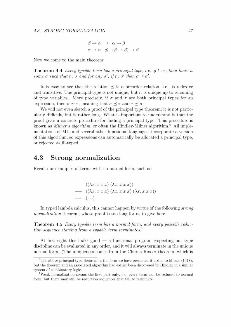
4.3. STRONG NORMALIZATION 47
β → α � α → β
α → α 6� (β → β) → β
Now we come to the main theorem:
Theorem 4.4 Every typable term has a principal type, i.e. if t : τ , then there issome σ such that t : σ and for any σ′, if t : σ′ then σ � σ′.
It is easy to see that the relation � is a preorder relation, i.e. is reflexiveand transitive. The principal type is not unique, but it is unique up to renamingof type variables. More precisely, if σ and τ are both principal types for anexpression, then σ ∼ τ , meaning that σ � τ and τ � σ.
We will not even sketch a proof of the principal type theorem; it is not partic-ularly difficult, but is rather long. What is important to understand is that theproof gives a concrete procedure for finding a principal type. This procedure isknown as Milner’s algorithm, or often the Hindley-Milner algorithm.6 All imple-mentations of ML, and several other functional languages, incorporate a versionof this algorithm, so expressions can automatically be allocated a principal type,or rejected as ill-typed.
4.3 Strong normalization
Recall our examples of terms with no normal form, such as:
((λx. x x x) (λx. x x x))
−→ ((λx. x x x) (λx. x x x) (λx. x x x))
−→ (· · ·)
In typed lambda calculus, this cannot happen by virtue of the following strongnormalization theorem, whose proof is too long for us to give here.
Theorem 4.5 Every typable term has a normal form, and every possible reduc-tion sequence starting from a typable term terminates.7
At first sight this looks good — a functional program respecting our typediscipline can be evaluated in any order, and it will always terminate in the uniquenormal form. (The uniqueness comes from the Church-Rosser theorem, which is
6The above principal type theorem in the form we have presented it is due to Milner (1978),but the theorem and an associated algorithm had earlier been discovered by Hindley in a similarsystem of combinatory logic.
7Weak normalization means the first part only, i.e. every term can be reduced to normalform, but there may still be reduction sequences that fail to terminate.
48 CHAPTER 4. TYPES
still true in the typed system.) However, the ability to write nonterminatingfunctions is essential to Turing completeness,8 so we are no longer able to defineall computable functions, not even all total ones.
This might not matter if we could define all ‘practically interesting’ functions.However this is not so; the class of functions definable as typed lambda termsis fairly limited. Schwichtenberg (1976) has proved that if Church numerals areused, then the definable functions are those that are polynomials or result frompolynomials using definition by cases. Note that this is strictly intensional: ifanother numeral representation is used, a different class of functions is obtained.In any case, it is not enough for a general programming language.
Since all definable functions are total, we are clearly unable to make arbitraryrecursive definitions. Indeed, the usual fixpoint combinators must be untypable;Y = λf. (λx. f(x x))(λx. f(x x)) clearly isn’t well-typed because it applies x toitself and x is bound by a lambda. In order to regain Turing-completeness wesimply add a way of defining arbitrary recursive functions that is well-typed. Weintroduce a polymorphic recursion operator with all types of the form:
Rec : ((σ → τ) → (σ → τ)) → σ → τ
and the extra reduction rule that for any F : (σ → τ) → (σ → τ) we have:
Rec F −→ F (Rec F )
From now on, we will suppose that recursive definitions, signalled by ‘let rec’,map down to the use of these recursion operators.
Further reading
Barendregt (1984) and Hindley and Seldin (1986) also consider typed lambdacalculus. The original paper by Milner (1978) is still a good source of informationabout polymorphic typing and the algorithm for finding principal types. A niceelementary treatment of typed lambda calculus, which gives a proof of StrongNormalization and discusses some interesting connections with logic, is Girard,Lafont, and Taylor (1989). This also discusses a more advanced version of typedlambda calculus called ‘System F’ where even though strong normalization holds,the majority of ‘interesting’ functions are definable.
Exercises
1. Is it true that if Γ ` t : σ then for any substitution θ we have Γ ` t : (σθ)?
8Given any recursive enumeration of total computable functions, we can always create onenot in the list by diagonalization. This will be illustrated in the Computability Theory course.

4.3. STRONG NORMALIZATION 49
2. Prove formally the type preservation theorems for α and β conversion.
3. Show that the converse to type preservation does not hold, i.e. it is possiblethat t −→ t′ and Γ ` t′ : σ but not Γ ` t : σ.
4. (*) Prove that every term of typed lambda calculus with principal type(α → α) → (α → α) reduces to a Church numeral.
5. (*) To what extent can the typechecking process be reversed, i.e. the terminferred from the type? For instance, is it true that in pure typed lambdacalculus with type variables but no constants and no recursion operator,that any t : α → β → α is in fact equal to K = λx y. x in the usual senseof lambda equality? If so, how far can this be generalized?9
6. (*) We will say that an arbitrary reduction relation −→ is weakly Church-Rosser if whenever t −→ t1 and t −→ t2, then there is a u with t1 −→∗ uand t2 −→∗ u, where −→∗ is the reflexive transitive closure of −→. ProveNewman’s Lemma, which states that if a relation is weakly Church-Rosserand obeys strong normalization, then −→∗ is Church-Rosser. (Hint: use aform of wellfounded induction.)10
9See Mairson (1991) for more on this question.10If you get stuck, there is a nice proof in Huet (1980).

Chapter 5
A taste of ML
In the last few chapters, we have started with pure lambda calculus and system-atically extended it with new primitive features. For example we added the ‘let’construct as primitive for the sake of making the polymorphic typing more useful,and a recursion operation in order to restore the computational power that waslost when adding types. By travelling further along this path, we will eventuallyarrive at ML, although it’s still valuable to retain the simple worldview of typedlambda calculus.
The next stage is to abandon the encodings of datatypes like booleans andnatural numbers via lambda terms, and instead make them primitive. That is, wehave new primitive types like bool and int (actually positive and negative inte-gers) and new type constructors like ×, a step we have in many ways anticipatedin the last chapter. Associated with these are new constants and new conversionrules. For example, the expression 2 + 2 is evaluated using machine arithmetic,rather than by translation into Church numerals and performing β-conversions.These additional conversions, regarded as augmenting the usual lambda opera-tions, are often referred to as ‘δ-conversions’. We will see in due course how theML language is extended in other ways in comparison with pure lambda calculus.First, we must address the fundamental question of ML’s evaluation strategy.
5.1 Eager evaluation
We have said that from a theoretical point of view, normal order (top downleft-to-right) reduction of expressions is to be preferred, since if any strategyterminates, this one will.1 However it has some practical defects. For example,consider the following:
(λx. x + x + x) (10 + 5)
1This strategy is familiar from a few traditional languages like Algol 60 where it is referredto as call by name.
50
5.1. EAGER EVALUATION 51
A normal order reduction results in (10 + 5) + (10 + 5) + (10 + 5), and thefollowing reduction steps need to evaluate three separate instances of the sameexpression. This is unacceptable in practice. There are two main solutions tothis problem, and these solutions divide the world of functional programminglanguages into two camps.
The first alternative is to stick with normal order reduction, but attemptto optimize the implementation so multiple subexpressions arising in this wayare shared, and never evaluated more than once. Internally, expressions arerepresented as directed acyclic graphs rather than as trees. This is known as lazyor call-by-need evaluation, since expressions are only evaluated when absolutelynecessary.
The second approach is to turn the theoretical considerations about reductionstrategy on their head and evaluate arguments to functions before passing thevalues to the function. This is known as applicative order or eager evaluation.The latter name arises because function arguments are evaluated even when theymay be unnecessary, e.g. t in (λx. y) t. Of course, eager evaluation means thatsome expressions may loop that would terminate in a lazy regime. But this isconsidered acceptable, since these instances are generally easy to avoid in practice.In any case, an eager evaluation strategy is the standard in many programminglanguages like C, where it is referred to as call by value.
ML adopts eager evaluation, for two main reasons. Choreographing the re-ductions and sharings that occur in lazy evaluation is quite tricky, and implemen-tations tend to be relatively inefficient and complicated. Unless the programmeris very careful, memory can fill up with pending unevaluated expressions, andin general it is hard to understand the space behaviour of programs. In factmany implementations of lazy evaluation try to optimize it to eager evaluationin cases where there is no semantic difference.2 By contrast, in ML, we alwaysfirst evaluate the arguments to functions and only then perform the β-reduction— this is simple and efficient, and is easy to implement using standard compilertechnology.
The second reason for preferring applicative order evaluation is that ML isnot a pure functional language, but includes imperative features (variables, as-signments etc.). Therefore the order of evaluation of subexpressions can make asemantic difference, rather than merely affecting efficiency. If lazy evaluation isused, it seems to become practically impossible for the programmer to visualize,in a nontrivial program, exactly when each subexpression gets evaluated. In theeager ML system, one just needs to remember the simple evaluation rule.
It is important to realize, however, that the ML evaluation strategy is notsimply bottom-up, the exact opposite of normal order reduction. In fact, MLnever evaluates underneath a lambda. (In particular, it never reduces η-redexes,
2They try to perform strictness analysis, a form of static analysis that can often discoverthat arguments are necessarily going to be evaluated (Mycroft 1981).

52 CHAPTER 5. A TASTE OF ML
only β-redexes.) In evaluating (λx. s[x]) t, t is evaluated first. However s[x] isnot touched since it is underneath a lambda, and any subexpressions of t thathappen to be in the scope of a lambda are also left alone. The precise evaluationrules are as follows:
• Constants evaluate to themselves.
• Evaluation stops immediately at λ-abstractions and does not look insidethem. In particular, there is no η-conversion.
• When evaluating a combination s t, then first both s and t are evaluated.Then, assuming that the evaluated form of s is a lambda abstraction, atoplevel β-conversion is performed and the process is repeated.
The order of evaluation of s and t varies between versions of ML. In theversion we will use, t is always evaluated first. Strictly, we should also specifya rule for let expressions, since as we have said they are by now accepted as aprimitive. However from the point of view of evaluation they can be understoodin the original way, as a lambda applied to an argument, with the understandingthat the rand will be evaluated first. To make this explicit, the rule for
let x = s in t
is that first of all s is evaluated, the resulting value is substituted for x in t, andfinally the new version of t is evaluated. Let us see some examples of evaluatingexpressions:
(λx. (λy. y + y) x)(2 + 2) −→ (λx. (λy. y + y) x)4
−→ (λy. y + y)4
−→ 4 + 4
−→ 8
Note that the subterm (λy. y + y) x is not reduced, since it is within the scopeof a lambda. However, terms that are reducible and not enclosed by a lambda inboth function and argument get reduced before the function application itself isevaluated, e.g. the second step in the following:
((λf x. f x) (λy. y + y)) (2 + 2) −→ ((λf x. f x) (λy. y + y)) 4
−→ (λx. (λy. y + y) x) 4
−→ (λy. y + y) 4
−→ 4 + 4
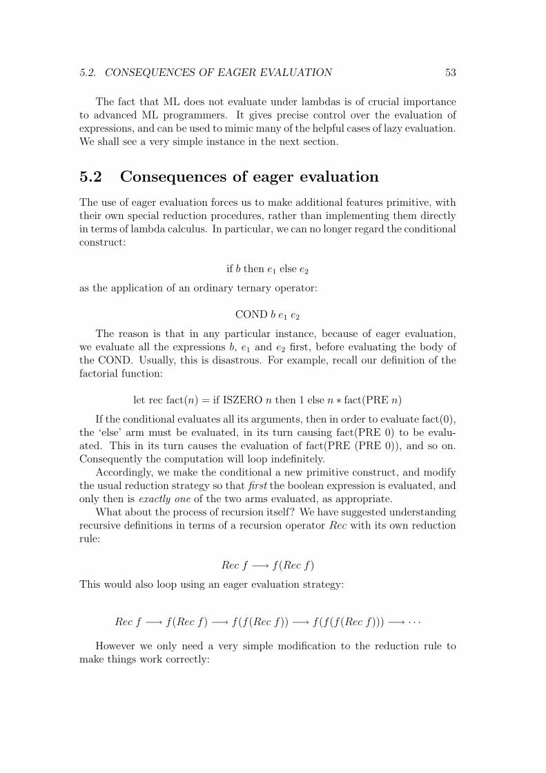
5.2. CONSEQUENCES OF EAGER EVALUATION 53
The fact that ML does not evaluate under lambdas is of crucial importanceto advanced ML programmers. It gives precise control over the evaluation ofexpressions, and can be used to mimic many of the helpful cases of lazy evaluation.We shall see a very simple instance in the next section.
5.2 Consequences of eager evaluation
The use of eager evaluation forces us to make additional features primitive, withtheir own special reduction procedures, rather than implementing them directlyin terms of lambda calculus. In particular, we can no longer regard the conditionalconstruct:
if b then e1 else e2
as the application of an ordinary ternary operator:
COND b e1 e2
The reason is that in any particular instance, because of eager evaluation,we evaluate all the expressions b, e1 and e2 first, before evaluating the body ofthe COND. Usually, this is disastrous. For example, recall our definition of thefactorial function:
let rec fact(n) = if ISZERO n then 1 else n ∗ fact(PRE n)
If the conditional evaluates all its arguments, then in order to evaluate fact(0),the ‘else’ arm must be evaluated, in its turn causing fact(PRE 0) to be evalu-ated. This in its turn causes the evaluation of fact(PRE (PRE 0)), and so on.Consequently the computation will loop indefinitely.
Accordingly, we make the conditional a new primitive construct, and modifythe usual reduction strategy so that first the boolean expression is evaluated, andonly then is exactly one of the two arms evaluated, as appropriate.
What about the process of recursion itself? We have suggested understandingrecursive definitions in terms of a recursion operator Rec with its own reductionrule:
Rec f −→ f(Rec f)
This would also loop using an eager evaluation strategy:
Rec f −→ f(Rec f) −→ f(f(Rec f)) −→ f(f(f(Rec f))) −→ · · ·
However we only need a very simple modification to the reduction rule tomake things work correctly:

54 CHAPTER 5. A TASTE OF ML
Rec f −→ f(λx. Rec f x)
Now the lambda on the right means that λx. Rec f x evaluates to itself, andso only after the expression has been further reduced following substitution inthe body of f will evaluation continue.
5.3 The ML family
We have been talking about ‘ML’ as if it were a single language. In fact thereare many variants of ML, even including ‘Lazy ML’, an implementation fromChalmers University in Sweden that is based on lazy evaluation. The most popu-lar version of ML in education is ‘Standard ML’, but we will use another version,called CAML (‘camel’) Light.3 We chose CAML Light for several reasons:
• The implementation is small and highly portable, so can be run effectivelyon Unix machines, PCs, Macs etc.
• The system is simple, syntactically and semantically, making it relativelyeasy to approach.
• The system is well suited to practical programming, e.g. it can easily beinterfaced to C and supports standard make-compatible separate compila-tion.
However, we will be teaching quite general techniques, and any code we writecan be run with a few minor syntactic changes in any version of ML, and indeedoften in other functional languages.
5.4 Starting up ML
ML has already been installed on Thor. In order to use it, you need to put theCAML binary directory on your PATH. This can be done (assuming you use the‘bash’ shell or one of its family), as follows:
PATH="$PATH:/home/jrh13/caml/bin"export PATH
To avoid doing this every time you log on, you can insert these lines near theend of your .bash profile, or the equivalent for your favourite shell. Now touse CAML in its normal interactive and interpretive mode, you simply need totype camllight, and the system should fire up and present its prompt (‘#’):
3The name stands for ‘Categorical Abstract Machine’, the underlying implementationmethod.

5.5. INTERACTING WITH ML 55
$ camllight> Caml Light version 0.73
#
In order to exit the system, simply type ctrl/d or quit();; at the prompt.If you are interested in installing CAML Light on your own machine, you shouldconsult the following Web page for detailed information:
http://pauillac.inria.fr/caml/
5.5 Interacting with ML
When ML presents you with its prompt, you can type in expressions, terminatedby two successive semicolons, and it will evaluate them and print the result. Incomputing jargon, the ML system sits in a read-eval-print loop: it repeatedlyreads an expression, evaluates it, and prints the result. For example, ML can beused as a simple calculator:
#10 + 5;;- : int = 15
The system not only returns the answer, but also the type of the expression,which it has inferred automatically. It can do this because it knows the typeof the built-in addition operator +. On the other hand, if an expression is nottypable, the system will reject it, and try to give some idea about how the typesfail to match up. In complicated cases, the error messages can be quite tricky tounderstand.
#1 + true;;Toplevel input:>let it = 1 + true;;> ^^^^This expression has type bool,but is used with type int.
Since ML is a functional language, expressions are allowed to have functiontype. The ML syntax for a lambda abstraction λx. t[x] is fun x -> t[x]. Forexample we can define the successor function:
#fun x -> x + 1;;- : int -> int = <fun>
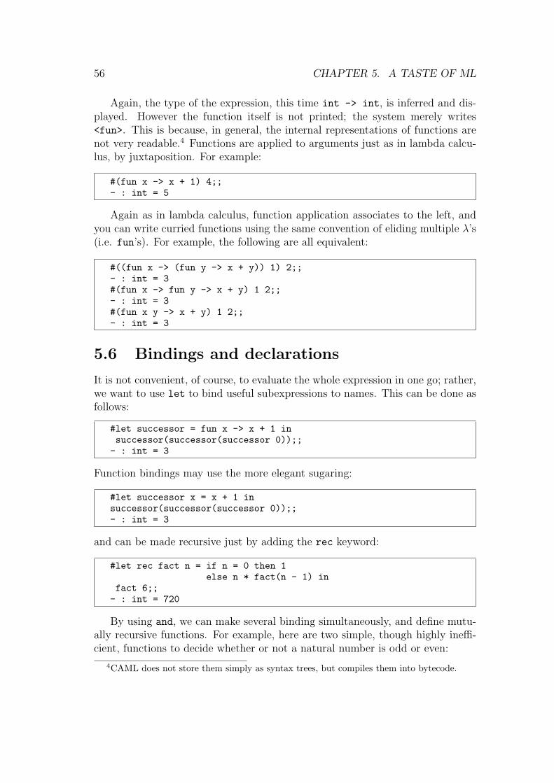
56 CHAPTER 5. A TASTE OF ML
Again, the type of the expression, this time int -> int, is inferred and dis-played. However the function itself is not printed; the system merely writes<fun>. This is because, in general, the internal representations of functions arenot very readable.4 Functions are applied to arguments just as in lambda calcu-lus, by juxtaposition. For example:
#(fun x -> x + 1) 4;;- : int = 5
Again as in lambda calculus, function application associates to the left, andyou can write curried functions using the same convention of eliding multiple λ’s(i.e. fun’s). For example, the following are all equivalent:
#((fun x -> (fun y -> x + y)) 1) 2;;- : int = 3#(fun x -> fun y -> x + y) 1 2;;- : int = 3#(fun x y -> x + y) 1 2;;- : int = 3
5.6 Bindings and declarations
It is not convenient, of course, to evaluate the whole expression in one go; rather,we want to use let to bind useful subexpressions to names. This can be done asfollows:
#let successor = fun x -> x + 1 insuccessor(successor(successor 0));;- : int = 3
Function bindings may use the more elegant sugaring:
#let successor x = x + 1 insuccessor(successor(successor 0));;- : int = 3
and can be made recursive just by adding the rec keyword:
#let rec fact n = if n = 0 then 1else n * fact(n - 1) in
fact 6;;- : int = 720
By using and, we can make several binding simultaneously, and define mutu-ally recursive functions. For example, here are two simple, though highly ineffi-cient, functions to decide whether or not a natural number is odd or even:
4CAML does not store them simply as syntax trees, but compiles them into bytecode.

5.6. BINDINGS AND DECLARATIONS 57
#let rec even n = if n = 0 then true else odd (n - 1)and odd n = if n = 0 then false else even (n - 1);;
even : int -> bool = <fun>odd : int -> bool = <fun>#even 12;;- : bool = true#odd 14;;- : bool = false
In fact, any bindings can be performed separately from the final application.ML remembers a set of variable bindings, and the user can add to that set inter-actively. Simply omit the in and terminate the phrase with a double semicolon:
#let successor = fun x -> x + 1;;successor : int -> int = <fun>
After this declaration, any later phrase may use the function successor, e.g:
#successor 11;;- : int = 12
Note that we are not making assignments to variables. Each binding is onlydone once when the system analyses the input; it cannot be repeated or modi-fied. It can be overwritten by a new definition using the same name, but this isnot assignment in the usual sense, since the sequence of events is only connectedwith the compilation process, not with the dynamics of program execution. In-deed, apart from the more interactive feedback from the system, we could equallyreplace all the double semicolons after the declarations by in and evaluate ev-erything at once. On this view we can see that the overwriting of a declarationreally corresponds to the definition of a new local variable that hides the outerone, according to the usual lambda calculus rules. For example:
#let x = 1;;x : int = 1#let y = 2;;y : int = 2#let x = 3;;x : int = 3#x + y;;- : int = 5
is the same as:
#let x = 1 inlet y = 2 inlet x = 3 inx + y;;- : int = 5

58 CHAPTER 5. A TASTE OF ML
Note carefully that, also following lambda calculus, variable binding is static,i.e. the first binding of x is still used until an inner binding occurs, and any usesof it until that point are not affected by the inner binding. For example:
#let x = 1;;x : int = 1#let f w = w + x;;f : int -> int = <fun>#let x = 2;;x : int = 2#f 0;;- : int = 1
The first version of LISP, however, used dynamic binding, where a rebindingof a variable propagated to earlier uses of the variable, so that the analogous se-quence to the above would return 2. This was in fact originally regarded as a bug,but soon programmers started to appreciate its convenience. It meant that whensome low-level function was modified, the change propagated automatically to allapplications of it in higher level functions, without the need for recompilation.The feature survived for a long time in many LISP dialects, but eventually theview that static binding is better prevailed. In Common LISP, static binding isthe default, but dynamic binding is available if desired via the keyword special.
5.7 Polymorphic functions
We can define polymorphic functions, like the identity operator:
#let I = fun x -> x;;I : ’a -> ’a = <fun>
ML prints type variables as ’a, ’b etc. These are supposed to be ASCIIrepresentations of α, β and so on. We can now use the polymorphic functionseveral times with different types:
#I true;;- : bool = true#I 1;;- : int = 1#I I I I 12;;- : int = 12
Each instance of I in the last expression has a different type, and intuitivelycorresponds to a different function. In fact, let’s define all the combinators:
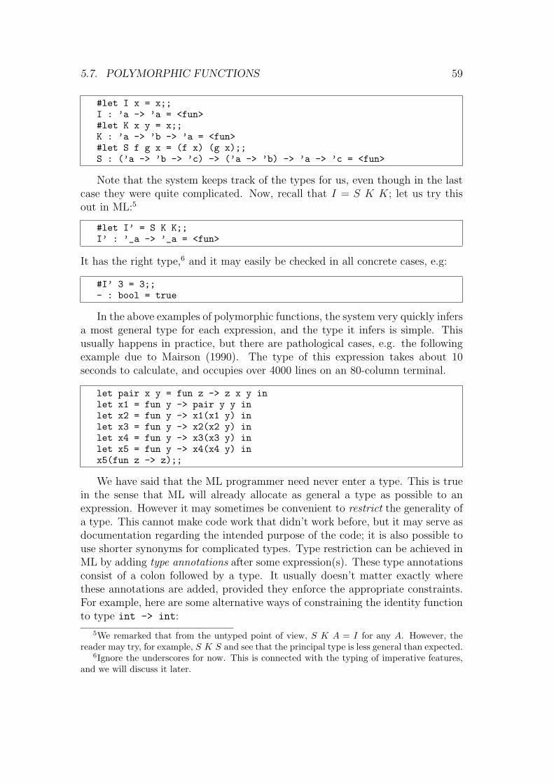
5.7. POLYMORPHIC FUNCTIONS 59
#let I x = x;;I : ’a -> ’a = <fun>#let K x y = x;;K : ’a -> ’b -> ’a = <fun>#let S f g x = (f x) (g x);;S : (’a -> ’b -> ’c) -> (’a -> ’b) -> ’a -> ’c = <fun>
Note that the system keeps track of the types for us, even though in the lastcase they were quite complicated. Now, recall that I = S K K; let us try thisout in ML:5
#let I’ = S K K;;I’ : ’_a -> ’_a = <fun>
It has the right type,6 and it may easily be checked in all concrete cases, e.g:
#I’ 3 = 3;;- : bool = true
In the above examples of polymorphic functions, the system very quickly infersa most general type for each expression, and the type it infers is simple. Thisusually happens in practice, but there are pathological cases, e.g. the followingexample due to Mairson (1990). The type of this expression takes about 10seconds to calculate, and occupies over 4000 lines on an 80-column terminal.
let pair x y = fun z -> z x y inlet x1 = fun y -> pair y y inlet x2 = fun y -> x1(x1 y) inlet x3 = fun y -> x2(x2 y) inlet x4 = fun y -> x3(x3 y) inlet x5 = fun y -> x4(x4 y) inx5(fun z -> z);;
We have said that the ML programmer need never enter a type. This is truein the sense that ML will already allocate as general a type as possible to anexpression. However it may sometimes be convenient to restrict the generality ofa type. This cannot make code work that didn’t work before, but it may serve asdocumentation regarding the intended purpose of the code; it is also possible touse shorter synonyms for complicated types. Type restriction can be achieved inML by adding type annotations after some expression(s). These type annotationsconsist of a colon followed by a type. It usually doesn’t matter exactly wherethese annotations are added, provided they enforce the appropriate constraints.For example, here are some alternative ways of constraining the identity functionto type int -> int:
5We remarked that from the untyped point of view, S K A = I for any A. However, thereader may try, for example, S K S and see that the principal type is less general than expected.
6Ignore the underscores for now. This is connected with the typing of imperative features,and we will discuss it later.

60 CHAPTER 5. A TASTE OF ML
#let I (x:int) = x;;I : int -> int = <fun>#let I x = (x:int);;I : int -> int = <fun>#let (I:int->int) = fun x -> x;;I : int -> int = <fun>#let I = fun (x:int) -> x;;I : int -> int = <fun>#let I = ((fun x -> x):int->int);;I : int -> int = <fun>
5.8 Equality of functions
Instead of comparing the actions of I and I ′ on particular arguments like 3, itwould seem that we can settle the matter definitively by comparing the functionsthemselves. However this doesn’t work:
#I’ = I;;Uncaught exception: Invalid_argument "equal: functional value"
It is in general forbidden to compare functions for equality, though a fewspecial instances, where the functions are obviously the same, yield true:
#let f x = x + 1;;f : int -> int = <fun>#let g x = x + 1;;g : int -> int = <fun>#f = f;;- : bool = true#f = g;;Uncaught exception: Invalid_argument "equal: functional value"#let h = g;;h : int -> int = <fun>#h = f;;Uncaught exception: Invalid_argument "equal: functional value"#h = g;;- : bool = true
Why these restrictions? Aren’t functions supposed to be first-class objects inML? Yes, but unfortunately, (extensional) function equality is not computable.This follows from a number of classic theorems in recursion theory, such as theunsolvability of the halting problem and Rice’s theorem.7 Let us give a concreteillustration of why this might be so. It is still an open problem whether the
7You will see these results proved in the Computation Theory course. Rice’s theorem is anextremely strong undecidability result which asserts that any nontrivial property of the functioncorresponding to a program is uncomputable from its text. An excellent computation theorytextbook is Davis, Sigal, and Weyuker (1994).

5.8. EQUALITY OF FUNCTIONS 61
following function terminates for all arguments, the assertion that it does beingknown as the Collatz conjecture:8
#let rec collatz n =if n <= 1 then 0else if even(n) then collatz(n / 2)else collatz(3 * n + 1);;
collatz : int -> int = <fun>
What is clear, though, is that if it does halt it returns 0. Now consider thefollowing trivial function:
#let f (x:int) = 0;;f : int -> int = <fun>
By deciding the equation collatz = f, the computer would settle the Collatzconjecture. It is easy to concoct other examples for open mathematical problems.
It is possible to trap out applications of the equality operator to functions anddatatypes built up from them as part of typechecking, rather than at runtime.Types that do not involve functions in these ways are known as equality types,since it is always valid to test objects of such types for equality. On the negativeside, this makes the type system much more complicated. However one mightargue that static typechecking should be extended as far as feasibility allows.
Further reading
Many books on functional programming bear on the general issues we have dis-cussed here, such as evaluation strategy. A good elementary introduction toCAML Light and functional programming is Mauny (1995). Paulson (1991) isanother good textbook, though based on Standard ML.
Exercises
1. Suppose that a ‘conditional’ function defined by ite(b,x,y) = if b then
x else y is the only function available that operates on arguments of typebool. Is there any way to write a factorial function?
2. Use the typing rules in the last chapter to write out a formal proof that theS combinator has the type indicated by the ML system.
8A good survey of this problem, and attempts to solve it, is given by Lagarias (1985).Strictly, we should use unlimited precision integers rather than machine arithmetic. We willsee later how to do this.

62 CHAPTER 5. A TASTE OF ML
3. Write a simple recursively defined function to perform exponentiation ofintegers, i.e. calculate xn for n ≥ 0. Write down two ML functions, theequality of which corresponds to the truth of Fermat’s last theorem: thereare no integers x, y, z and natural number n > 2 with xn + yn = zn exceptfor the trivial case where x = 0 or y = 0.
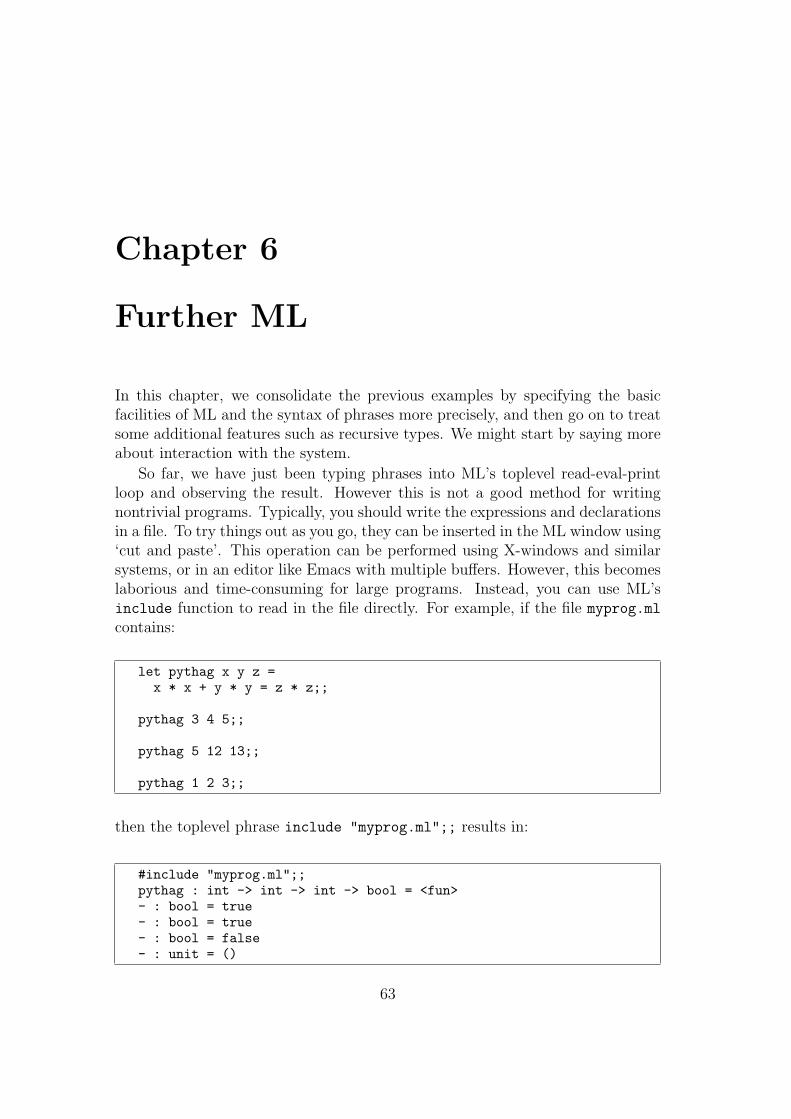
Chapter 6
Further ML
In this chapter, we consolidate the previous examples by specifying the basicfacilities of ML and the syntax of phrases more precisely, and then go on to treatsome additional features such as recursive types. We might start by saying moreabout interaction with the system.
So far, we have just been typing phrases into ML’s toplevel read-eval-printloop and observing the result. However this is not a good method for writingnontrivial programs. Typically, you should write the expressions and declarationsin a file. To try things out as you go, they can be inserted in the ML window using‘cut and paste’. This operation can be performed using X-windows and similarsystems, or in an editor like Emacs with multiple buffers. However, this becomeslaborious and time-consuming for large programs. Instead, you can use ML’sinclude function to read in the file directly. For example, if the file myprog.ml
contains:
let pythag x y z =x * x + y * y = z * z;;
pythag 3 4 5;;
pythag 5 12 13;;
pythag 1 2 3;;
then the toplevel phrase include "myprog.ml";; results in:
#include "myprog.ml";;pythag : int -> int -> int -> bool = <fun>- : bool = true- : bool = true- : bool = false- : unit = ()
63

64 CHAPTER 6. FURTHER ML
That is, the ML system responds just as if the phrases had been entered atthe top level. The final line is the result of evaluating the include expressionitself.
In large programs, it is often helpful to include comments. In ML, these arewritten between the symbols (* and *), e.g.
(* ------------------------------------------------------ *)(* This function tests if (x,y,z) is a Pythagorean triple *)(* ------------------------------------------------------ *)
let pythag x y z =x * x + y * y = z * z;;
(*comments*) pythag (*can*) 3 (*go*) 4 (*almost*) 5 (*anywhere*)(* and (* can (* be (* nested *) quite *) arbitrarily *) *);;
6.1 Basic datatypes and operations
ML features several built-in primitive types. From these, composite types maybe built using various type constructors. For the moment, we will only use thefunction space constructor -> and the Cartesian product constructor *, but wewill see in due course which others are provided, and how to define new typesand type constructors. The primitive types that concern us now are:
• The type unit. This is a 1-element type, whose only element is written(). Obviously, something of type unit conveys no information, so it iscommonly used as the return type of imperatively written ‘functions’ thatperform a side-effect, such as include above. It is also a convenient argu-ment where the only use of a function type is to delay evaluation.
• The type bool. This is a 2-element type of booleans (truth-values) whoseelements are written true and false.
• The type int. This contains some finite subset of the positive and negativeintegers. Typically the permitted range is from −230 (−1073741824) up to230−1 (1073741823).1 The numerals are written in the usual way, optionallywith a negation sign, e.g. 0, 32, -25.
• The type string contains strings (i.e. finite sequences) of characters. Theyare written and printed between double quotes, e.g. "hello". In order toencode include special characters in strings, C-like escape sequences areused. For example, \" is the double quote itself, and \n is the newlinecharacter.
1This is even more limited than expected for machine arithmetic because a bit is stolen forthe garbage collector. We will see later how to use an alternative type of integers with unlimitedprecision.

6.1. BASIC DATATYPES AND OPERATIONS 65
The above values like (), false, 7 and "caml" are all to be regarded asconstants in the lambda calculus sense. There are other constants correspondingto operations on the basic types. Some of these may be written as infix operators,for the sake of familiarity. These have a notion of precedence so that expressionsare grouped together as one would expect. For example, we write x + y ratherthan + x y and x < 2 * y + z rather than < x (+ (* 2 y) z). The logicaloperator not also has a special parsing status, in that the usual left-associativityrule is reversed for it: not not p means not (not p). User-defined functionsmay be granted infix status via the #infix directive. For example, here is adefinition of a function performing composition of functions:
#let successor x = x + 1;;successor : int -> int = <fun>#let o f g = fun x -> f(g x);;o : (’a -> ’b) -> (’c -> ’a) -> ’c -> ’b = <fun>#let add3 = o successor (o successor successor);;add3 : int -> int = <fun>#add3 0;;- : int = 3##infix "o";;#let add3’ = successor o successor o successor;;add3’ : int -> int = <fun>#add3’ 0;;- : int = 3
It is not possible to specify the precedence of user-defined infixes, nor to makeuser-defined non-infix functions right-associative. Note that the implicit opera-tion of ‘function application’ has a higher precedence than any binary operator,so successor 1 * 2 parses as (successor 1) * 2. If it is desired to use a func-tion with special status as an ordinary constant, simply precede it by prefix.For example:
#o successor successor;;Toplevel input:>o successor successor;;>^Syntax error.#prefix o successor successor;;- : int -> int = <fun>#(prefix o) successor successor;;- : int -> int = <fun>
With these questions of concrete syntax out of the way, let us present asystematic list of the operators on the basic types above. The unary operatorsare:
Operator Type Meaning- int -> int Numeric negationnot bool -> bool Logical negation

66 CHAPTER 6. FURTHER ML
and the binary operators, in approximately decreasing order of precedence, are:
Operator Type Meaningmod int -> int -> int Modulus (remainder)* int -> int -> int Multiplication/ int -> int -> int Truncating division+ int -> int -> int Addition- int -> int -> int Subtraction^ string -> string -> string String concatenation= ’a -> ’a -> bool Equality<> ’a -> ’a -> bool Inequality< ’a -> ’a -> bool Less than<= ’a -> ’a -> bool Less than or equal> ’a -> ’a -> bool Greater than>= ’a -> ’a -> bool Greater than or equal& bool -> bool -> bool Boolean ‘and’or bool -> bool -> bool Boolean ‘or’
For example, x > 0 & x < 1 is parsed as & (> x 0) (< x 1). Note thatall the comparisons, not just the equality relation, are polymorphic. They notonly order integers in the expected way, and strings alphabetically, but all otherprimitive types and composite types in a fairly natural way. Once again, however,they are not in general allowed to be used on functions.
The two boolean operations & and or have their own special evaluation strat-egy, like the conditional expression. In fact, they can be regarded as synonymsfor conditional expressions:
p & q4= if p then q else false
p or q4= if p then true else q
Thus, the ‘and’ operation evaluates its first argument, and only if it is true,evaluates its second. Conversely, the ‘or’ operation evaluates its first argument,and only if it is false evaluates its second.
6.2 Syntax of ML phrases
Expressions in ML can be built up from constants and variables; any identifierthat is not currently bound is treated as a variable. Declarations bind namesto values of expressions, and declarations can occur locally inside expressions.Thus, the syntax classes of expressions and declarations are mutually recursive.We can represent this by the following BNF grammar.2
2We neglect many constructs that we won’t be concerned with. A few will be introducedlater. See the CAML manual for full details.
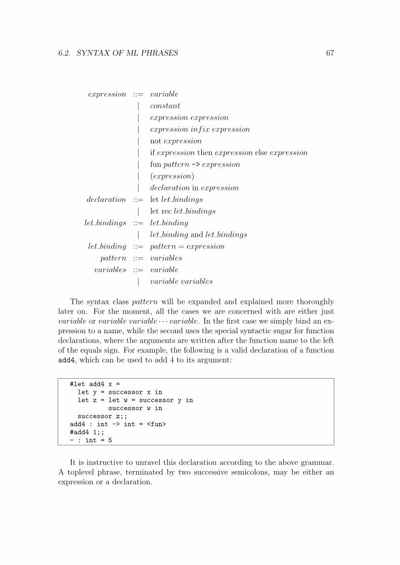
6.2. SYNTAX OF ML PHRASES 67
expression ::= variable
| constant
| expression expression
| expression infix expression
| not expression
| if expression then expression else expression
| fun pattern -> expression
| (expression)
| declaration in expression
declaration ::= let let bindings
| let rec let bindings
let bindings ::= let binding
| let binding and let bindings
let binding ::= pattern = expression
pattern ::= variables
variables ::= variable
| variable variables
The syntax class pattern will be expanded and explained more thoroughlylater on. For the moment, all the cases we are concerned with are either justvariable or variable variable · · · variable. In the first case we simply bind an ex-pression to a name, while the second uses the special syntactic sugar for functiondeclarations, where the arguments are written after the function name to the leftof the equals sign. For example, the following is a valid declaration of a functionadd4, which can be used to add 4 to its argument:
#let add4 x =let y = successor x inlet z = let w = successor y in
successor w insuccessor z;;
add4 : int -> int = <fun>#add4 1;;- : int = 5
It is instructive to unravel this declaration according to the above grammar.A toplevel phrase, terminated by two successive semicolons, may be either anexpression or a declaration.

68 CHAPTER 6. FURTHER ML
6.3 Further examples
It is easy to define by recursion a function that takes a positive integer n and afunction f and returns fn, i.e. f ◦ · · · ◦ f (n times):
#let rec funpow n f x =if n = 0 then xelse funpow (n - 1) f (f x);;
funpow : int -> (’a -> ’a) -> ’a -> ’a = <fun>
In fact, a little thought will show that the function funpow takes a machineinteger n and returns the Church numeral corresponding to n. Since functionsaren’t printed, we can’t actually look at the lambda expression representing aChurch numeral:
#funpow 6;;- : (’_a -> ’_a) -> ’_a -> ’_a = <fun>
However it is straightforward to define an inverse function to funpow thattakes a Church numeral back to a machine integer:
#let defrock n = n (fun x -> x + 1) 0;;defrock : ((int -> int) -> int -> ’a) -> ’a = <fun>#defrock(funpow 32);;- : int = 32
We can try out some of the arithmetic operations on Church numerals:
#let add m n f x = m f (n f x);;add : (’a -> ’b -> ’c) -> (’a -> ’d -> ’b) -> ’a -> ’d -> ’c = <fun>#let mul m n f x = m (n f) x;;mul : (’a -> ’b -> ’c) -> (’d -> ’a) -> ’d -> ’b -> ’c = <fun>#let exp m n f x = n m f x;;exp : ’a -> (’a -> ’b -> ’c -> ’d) -> ’b -> ’c -> ’d = <fun>#let test bop x y = defrock (bop (funpow x) (funpow y));;test :(((’a -> ’a) -> ’a -> ’a) ->((’b -> ’b) -> ’b -> ’b) -> (int -> int) -> int -> ’c) ->int -> int -> ’c = <fun>
#test add 2 10;;- : int = 12#test mul 2 10;;- : int = 20#test exp 2 10;;- : int = 1024
The above is not a very efficient way of performing arithmetic operations.ML does not have a function for exponentiation, but it is easy to define one byrecursion:
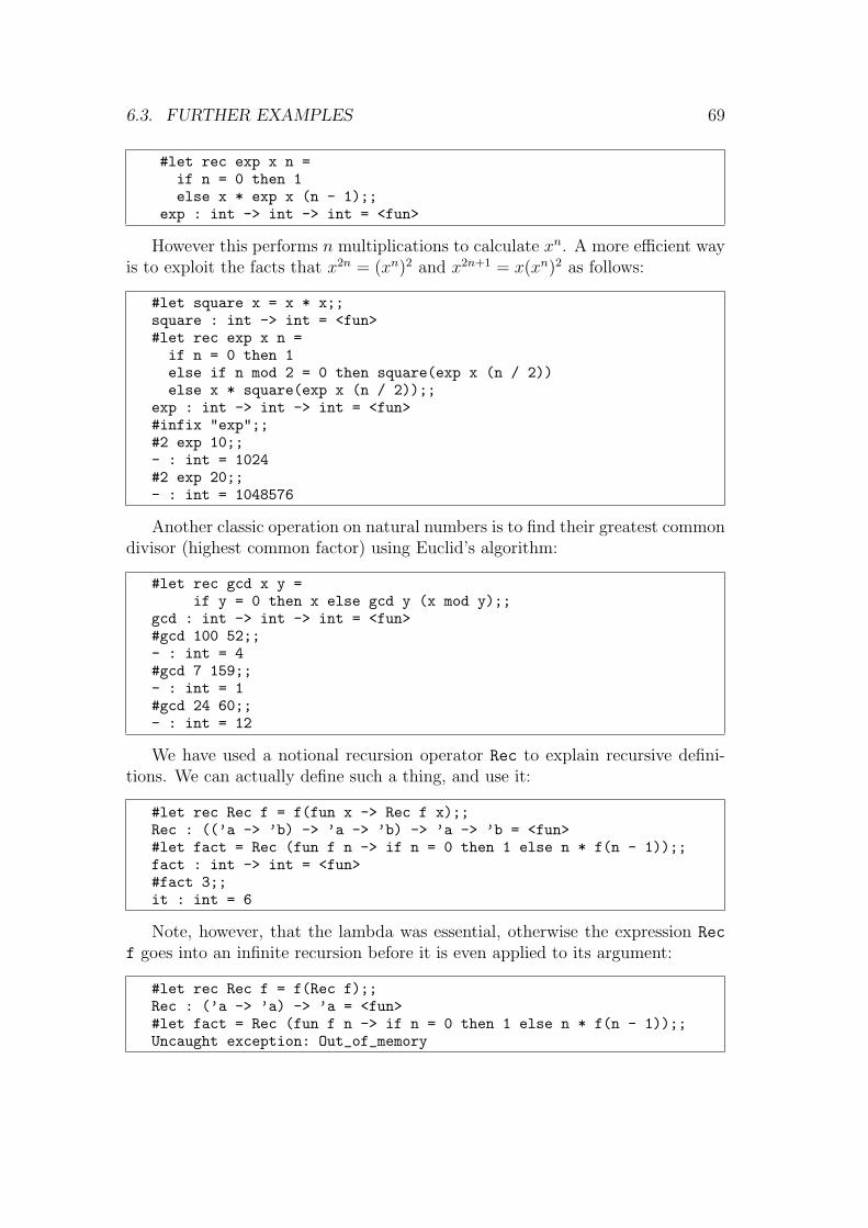
6.3. FURTHER EXAMPLES 69
#let rec exp x n =if n = 0 then 1else x * exp x (n - 1);;
exp : int -> int -> int = <fun>
However this performs n multiplications to calculate xn. A more efficient wayis to exploit the facts that x2n = (xn)2 and x2n+1 = x(xn)2 as follows:
#let square x = x * x;;square : int -> int = <fun>#let rec exp x n =if n = 0 then 1else if n mod 2 = 0 then square(exp x (n / 2))else x * square(exp x (n / 2));;
exp : int -> int -> int = <fun>#infix "exp";;#2 exp 10;;- : int = 1024#2 exp 20;;- : int = 1048576
Another classic operation on natural numbers is to find their greatest commondivisor (highest common factor) using Euclid’s algorithm:
#let rec gcd x y =if y = 0 then x else gcd y (x mod y);;
gcd : int -> int -> int = <fun>#gcd 100 52;;- : int = 4#gcd 7 159;;- : int = 1#gcd 24 60;;- : int = 12
We have used a notional recursion operator Rec to explain recursive defini-tions. We can actually define such a thing, and use it:
#let rec Rec f = f(fun x -> Rec f x);;Rec : ((’a -> ’b) -> ’a -> ’b) -> ’a -> ’b = <fun>#let fact = Rec (fun f n -> if n = 0 then 1 else n * f(n - 1));;fact : int -> int = <fun>#fact 3;;it : int = 6
Note, however, that the lambda was essential, otherwise the expression Rec
f goes into an infinite recursion before it is even applied to its argument:
#let rec Rec f = f(Rec f);;Rec : (’a -> ’a) -> ’a = <fun>#let fact = Rec (fun f n -> if n = 0 then 1 else n * f(n - 1));;Uncaught exception: Out_of_memory

70 CHAPTER 6. FURTHER ML
6.4 Type definitions
We have promised that ML has facilities for declaring new type constructors,so that composite types can be built up out of existing ones. In fact, ML goesfurther and allows a composite type to be built up not only out of preexistingtypes but also from the composite type itself. Such types, naturally enough, aresaid to be recursive. They are declared using the type keyword followed by anequation indicating how the new type is built up from existing ones and itself.We will illustrate this by a few examples. The first one is the definition of a sumtype, intended to correspond to the disjoint union of two existing types.
#type (’a,’b)sum = inl of ’a | inr of ’b;;Type sum defined.
Roughly, an object of type (’a,’b)sum is either something of type ’a orsomething of type ’b. More formally, however, all these things have differenttypes. The type declaration also declares the so-called constructors inl and inr.These are functions that take objects of the component types and inject theminto the new type. Indeed, we can see their types in the ML system and applythem to objects:
#inl;;- : ’a -> (’a, ’b) sum = <fun>#inr;;- : ’a -> (’b, ’a) sum = <fun>#inl 5;;- : (int, ’a) sum = inl 5#inr false;;- : (’a, bool) sum = inr false
We can visualize the situation via the following diagram. Given two existingtypes α and β, the type (α, β)sum is composed precisely of separate copies of αand β, and the two constructors map onto the respective copies:
α
β
(α, β)sum
�������������:
inl
inr
XXXXXXXXXXXXXz
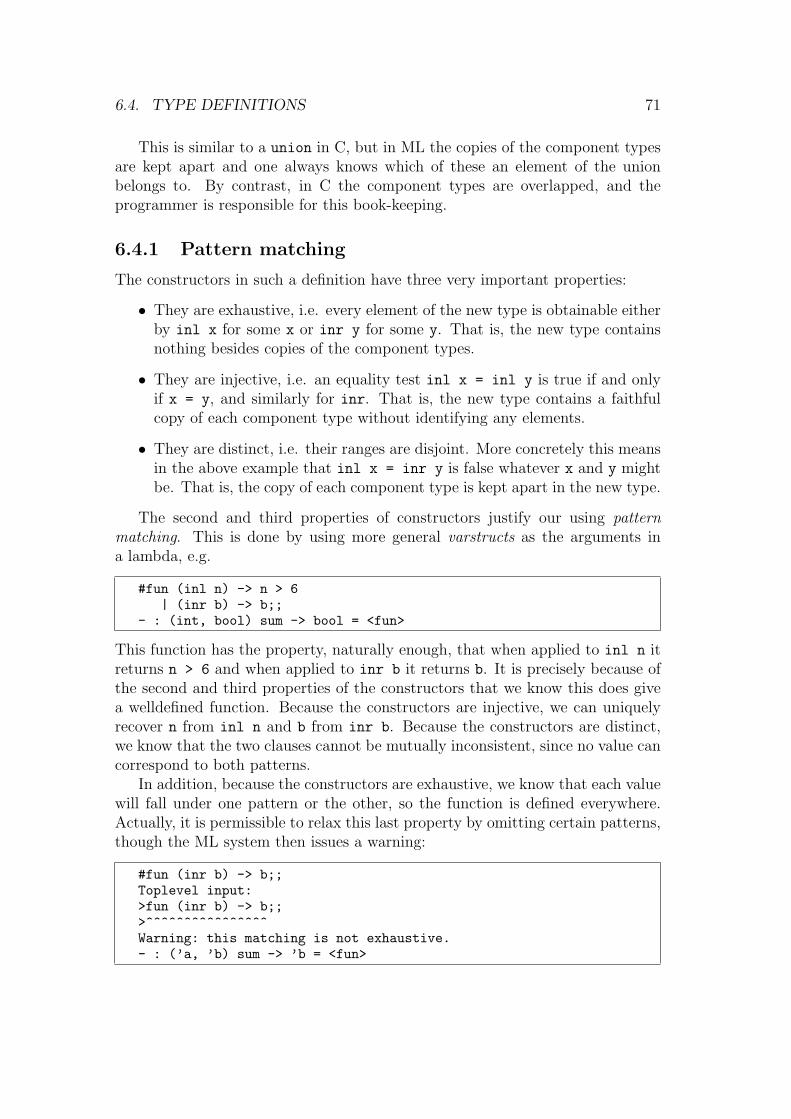
6.4. TYPE DEFINITIONS 71
This is similar to a union in C, but in ML the copies of the component typesare kept apart and one always knows which of these an element of the unionbelongs to. By contrast, in C the component types are overlapped, and theprogrammer is responsible for this book-keeping.
6.4.1 Pattern matching
The constructors in such a definition have three very important properties:
• They are exhaustive, i.e. every element of the new type is obtainable eitherby inl x for some x or inr y for some y. That is, the new type containsnothing besides copies of the component types.
• They are injective, i.e. an equality test inl x = inl y is true if and onlyif x = y, and similarly for inr. That is, the new type contains a faithfulcopy of each component type without identifying any elements.
• They are distinct, i.e. their ranges are disjoint. More concretely this meansin the above example that inl x = inr y is false whatever x and y mightbe. That is, the copy of each component type is kept apart in the new type.
The second and third properties of constructors justify our using patternmatching. This is done by using more general varstructs as the arguments ina lambda, e.g.
#fun (inl n) -> n > 6| (inr b) -> b;;
- : (int, bool) sum -> bool = <fun>
This function has the property, naturally enough, that when applied to inl n itreturns n > 6 and when applied to inr b it returns b. It is precisely because ofthe second and third properties of the constructors that we know this does givea welldefined function. Because the constructors are injective, we can uniquelyrecover n from inl n and b from inr b. Because the constructors are distinct,we know that the two clauses cannot be mutually inconsistent, since no value cancorrespond to both patterns.
In addition, because the constructors are exhaustive, we know that each valuewill fall under one pattern or the other, so the function is defined everywhere.Actually, it is permissible to relax this last property by omitting certain patterns,though the ML system then issues a warning:
#fun (inr b) -> b;;Toplevel input:>fun (inr b) -> b;;>^^^^^^^^^^^^^^^^Warning: this matching is not exhaustive.- : (’a, ’b) sum -> ’b = <fun>
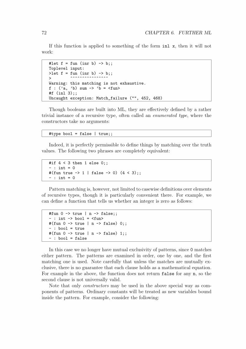
72 CHAPTER 6. FURTHER ML
If this function is applied to something of the form inl x, then it will notwork:
#let f = fun (inr b) -> b;;Toplevel input:>let f = fun (inr b) -> b;;> ^^^^^^^^^^^^^^^^Warning: this matching is not exhaustive.f : (’a, ’b) sum -> ’b = <fun>#f (inl 3);;Uncaught exception: Match_failure ("", 452, 468)
Though booleans are built into ML, they are effectively defined by a rathertrivial instance of a recursive type, often called an enumerated type, where theconstructors take no arguments:
#type bool = false | true;;
Indeed, it is perfectly permissible to define things by matching over the truthvalues. The following two phrases are completely equivalent:
#if 4 < 3 then 1 else 0;;- : int = 0#(fun true -> 1 | false -> 0) (4 < 3);;- : int = 0
Pattern matching is, however, not limited to casewise definitions over elementsof recursive types, though it is particularly convenient there. For example, wecan define a function that tells us whether an integer is zero as follows:
#fun 0 -> true | n -> false;;- : int -> bool = <fun>#(fun 0 -> true | n -> false) 0;;- : bool = true#(fun 0 -> true | n -> false) 1;;- : bool = false
In this case we no longer have mutual exclusivity of patterns, since 0 matcheseither pattern. The patterns are examined in order, one by one, and the firstmatching one is used. Note carefully that unless the matches are mutually ex-clusive, there is no guarantee that each clause holds as a mathematical equation.For example in the above, the function does not return false for any n, so thesecond clause is not universally valid.
Note that only constructors may be used in the above special way as com-ponents of patterns. Ordinary constants will be treated as new variables boundinside the pattern. For example, consider the following:
6.4. TYPE DEFINITIONS 73
#let true_1 = true;;true_1 : bool = true#let false_1 = false;;false_1 : bool = false#(fun true_1 -> 1 | false_1 -> 0) (4 < 3);;Toplevel input:>(fun true_1 -> 1 | false_1 -> 0) (4 < 3);;> ^^^^^^^Warning: this matching case is unused.- : int = 1
In general, the unit element (), the truth values, the integer numerals, thestring constants and the pairing operation (infix comma) have constructor status,as well as other constructors from predefined recursive types. When they occurin a pattern the target value must correspond. All other identifiers match anyexpression and in the process become bound.
As well as the varstructs in lambda expressions, there are other ways of per-forming pattern matching. Instead of creating a function via pattern matchingand applying it to an expression, one can perform pattern-matching over theexpression directly using the following construction:
match expression with pattern1->E1 | · · · | patternn->En
The simplest alternative of all is to use
let pattern = expression
but in this case only a single pattern is allowed.
6.4.2 Recursive types
The previous examples have all been recursive only vacuously, in that we havenot defined a type in terms of itself. For a more interesting example, we willdeclare a type of lists (finite ordered sequences) of elements of type ’a.
#type (’a)list = Nil | Cons of ’a * (’a)list;;Type list defined.
Let us examine the types of the constructors:
#Nil;;- : ’a list = Nil#Cons;;- : ’a * ’a list -> ’a list = <fun>

74 CHAPTER 6. FURTHER ML
The constructor Nil, which takes no arguments, simply creates some object oftype (’a)list which is to be thought of as the empty list. The other constructorCons takes an element of type ’a and an element of the new type (’a)list andgives another, which we think of as arising from the old list by adding one elementto the front of it. For example, we can consider the following:
#Nil;;- : ’a list = Nil#Cons(1,Nil);;- : int list = Cons (1, Nil)#Cons(1,Cons(2,Nil));;- : int list = Cons (1, Cons (2, Nil))#Cons(1,Cons(2,Cons(3,Nil)));;- : int list = Cons (1, Cons (2, Cons (3, Nil)))
Because the constructors are distinct and injective, it is easy to see thatall these values, which we think of as lists [], [1], [1; 2] and [1; 2; 3], are distinct.Indeed, purely from these properties of the constructors, it follows that arbitrarilylong lists of elements may be encoded in the new type. Actually, ML already hasa type list just like this one defined. The only difference is syntactic: the emptylist is written [] and the recursive constructor ::, has infix status. Thus, theabove lists are actually written:
#[];;- : ’a list = []#1::[];;- : int list = [1]#1::2::[];;- : int list = [1; 2]#1::2::3::[];;- : int list = [1; 2; 3]
The lists are printed in an even more natural notation, and this is also allowedfor input. Nevertheless, when the exact expression in terms of constructors isneeded, it must be remembered that this is only a surface syntax. For example,we can define functions to take the head and tail of a list, using pattern matching.
#let hd (h::t) = h;;Toplevel input:>let hd (h::t) = h;;> ^^^^^^^^^^^^^Warning: this matching is not exhaustive.hd : ’a list -> ’a = <fun>#let tl (h::t) = t;;Toplevel input:>let tl (h::t) = t;;> ^^^^^^^^^^^^^Warning: this matching is not exhaustive.tl : ’a list -> ’a list = <fun>
6.4. TYPE DEFINITIONS 75
The compiler warns us that these both fail when applied to the empty list,since there is no pattern to cover it (remember that the constructors are distinct).Let us see them in action:
#hd [1;2;3];;- : int = 1#tl [1;2;3];;- : int list = [2; 3]#hd [];;Uncaught exception: Match_failure
Note that the following is not a correct definition of hd. In fact, it constrainsthe input list to have exactly two elements for matching to succeed, as can beseen by thinking of the version in terms of the constructors:
#let hd [x;y] = x;;Toplevel input:>let hd [x;y] = x;;> ^^^^^^^^^^^^Warning: this matching is not exhaustive.hd : ’a list -> ’a = <fun>#hd [5;6];;- : int = 5#hd [5;6;7];;Uncaught exception: Match_failure
Pattern matching can be combined with recursion. For example, here is afunction to return the length of a list:
#let rec length =fun [] -> 0| (h::t) -> 1 + length t;;
length : ’a list -> int = <fun>#length [];;- : int = 0#length [5;3;1];;- : int = 3
Alternatively, this can be written in terms of our earlier ‘destructor’ functionshd and tl:
#let rec length l =if l = [] then 0else 1 + length(tl l);;
This latter style of function definition is more usual in many languages, no-tably LISP, but the direct use of pattern matching is often more elegant.
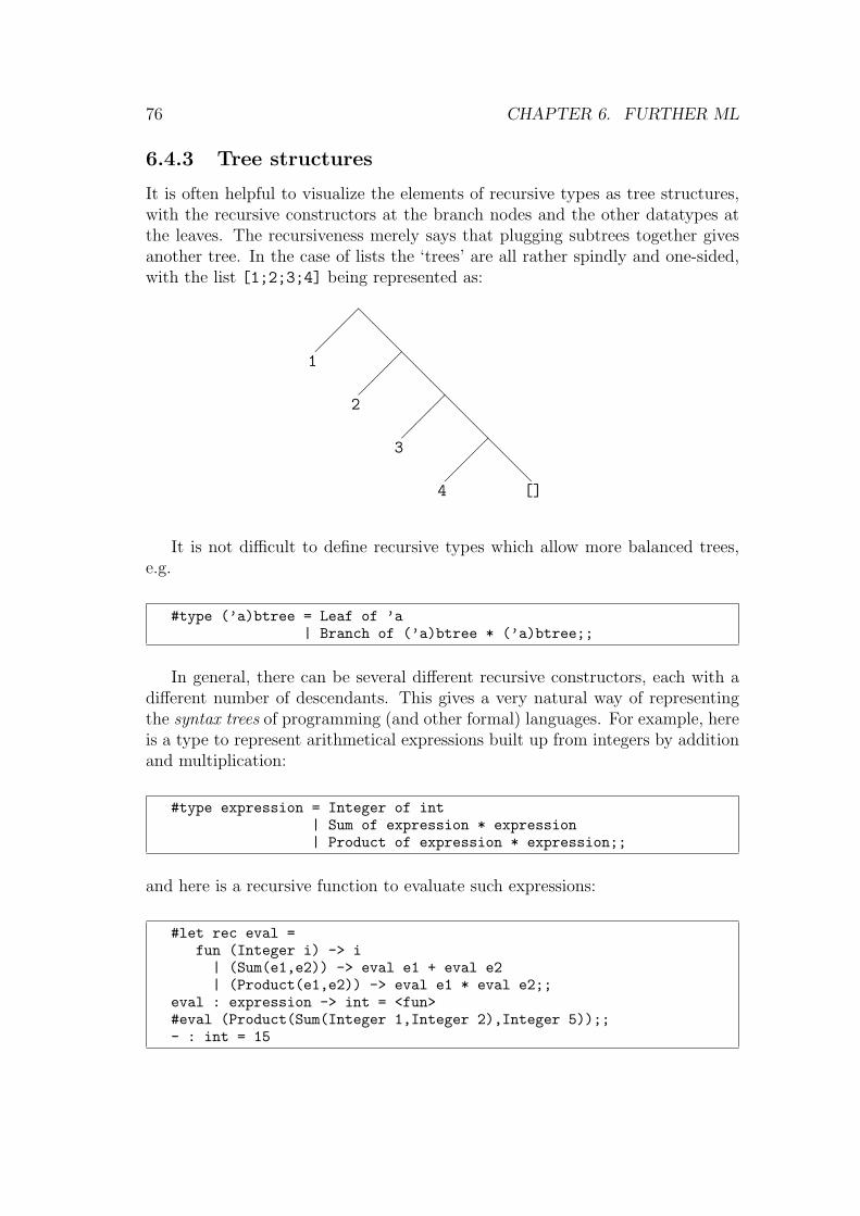
76 CHAPTER 6. FURTHER ML
6.4.3 Tree structures
It is often helpful to visualize the elements of recursive types as tree structures,with the recursive constructors at the branch nodes and the other datatypes atthe leaves. The recursiveness merely says that plugging subtrees together givesanother tree. In the case of lists the ‘trees’ are all rather spindly and one-sided,with the list [1;2;3;4] being represented as:
��
�
@@
@@
@@
��
�@
@@
��
�@
@@
��
�
1
2
3
4 []
It is not difficult to define recursive types which allow more balanced trees,e.g.
#type (’a)btree = Leaf of ’a| Branch of (’a)btree * (’a)btree;;
In general, there can be several different recursive constructors, each with adifferent number of descendants. This gives a very natural way of representingthe syntax trees of programming (and other formal) languages. For example, hereis a type to represent arithmetical expressions built up from integers by additionand multiplication:
#type expression = Integer of int| Sum of expression * expression| Product of expression * expression;;
and here is a recursive function to evaluate such expressions:
#let rec eval =fun (Integer i) -> i| (Sum(e1,e2)) -> eval e1 + eval e2| (Product(e1,e2)) -> eval e1 * eval e2;;
eval : expression -> int = <fun>#eval (Product(Sum(Integer 1,Integer 2),Integer 5));;- : int = 15

6.4. TYPE DEFINITIONS 77
Such abstract syntax trees are a useful representation which allows all sorts ofmanipulations. Often the first step programming language compilers and relatedtools take is to translate the input text into an ‘abstract syntax tree’ accordingto the parsing rules. Note that conventions such as precedences and bracketingsare not needed once we have reached the level of abstract syntax; the tree struc-ture makes these explicit. We will use such techniques to write ML versions ofthe formal rules of lambda calculus that we were considering earlier. First, thefollowing type is used to represent lambda terms:
#type term = Var of string| Const of string| Comb of term * term| Abs of string * term;;
Type term defined.
Note that we make Abs take a variable name and a term rather than twoterms in order to prohibit the formation of terms that aren’t valid. For example,we represent the term λx y. y (x x y) by:
Abs("x",Abs("y",Comb(Var "y",Comb(Comb(Var "x",Var "x"),Var "y"))))
Here is the recursive definition of a function free in to decide whether avariable is free in a term:
#let rec free_in x =fun (Var v) -> x = v| (Const c) -> false| (Comb(s,t)) -> free_in x s or free_in x t| (Abs(v,t)) -> not x = v & free_in x t;;
free_in : string -> term -> bool = <fun>#free_in "x" (Comb(Var "f",Var "x"));;- : bool = true#free_in "x" (Abs("x",Comb(Var "x",Var "y")));;- : bool = false
Similarly, we can define substitution by recursion. First, though, we needa function to rename variables to avoid name clashes. We want the ability toconvert an existing variable name to a new one that is not free in some givenexpression. The renaming is done by adding prime characters.
#let rec variant x t =if free_in x t then variant (x^"’") telse x;;
variant : string -> term -> string = <fun>#variant "x" (Comb(Var "f",Var "x"));;- : string = "x’"#variant "x" (Abs("x",Comb(Var "x",Var "y")));;- : string = "x"#variant "x" (Comb(Var "f",Comb(Var "x",Var "x’")));;- : string = "x’’"
78 CHAPTER 6. FURTHER ML
Now we can define substitution just as we did in abstract terms:
#let rec subst u (t,x) =match u withVar y -> if x = y then t else Var y
| Const c -> Const c| Comb(s1,s2) -> Comb(subst s1 (t,x),subst s2 (t,x))| Abs(y,s) -> if x = y then Abs(y,s)
else if free_in x s & free_in y t thenlet z = variant y (Comb(s,t)) inAbs(z,subst (subst s (Var y,z)) (t,x))
else Abs(y,subst s (t,x));;subst : term -> term * string -> term = <fun>
Note the very close parallels between the standard mathematical presentationof lambda calculus, as we presented earlier, and the ML version here. All we reallyneed to make the analogy complete is a means of reading and writing the termsin some more readable form, rather than by explicitly invoking the constructors.We will return to this issue later, and see how to add these features.
6.4.4 The subtlety of recursive types
A recursive type may contain nested instances of other type constructors, includ-ing the function space constructor. For example, consider the following:
#type (’a)embedding = K of (’a)embedding->’a;;Type embedding defined.
If we stop to think about the underlying semantics, this looks disquieting.Consider for example the special case when ’a is bool. We then have an injec-tive function K:((bool)embedding->bool)->(bool)embedding. This directlycontradicts Cantor’s theorem that the set of all subsets of X cannot be injectedinto X.3 Hence we need to be more careful with the semantics of types. Infact α → β cannot be interpreted as the full function space, or recursive typeconstructions like the above are inconsistent. However, since all functions wecan actually create are computable, it is reasonable to restrict ourselves to com-putable functions only. With that restriction, a consistent semantics is possible,although the details are complicated.
The above definition also has interesting consequences for the type system.For example, we can now define the Y combinator, by using K as a kind of typecast. Note that if the Ks are deleted, this is essentially the usual definition of
3Proof: consider C = {i(s) | s ∈ ℘(X) and i(s) 6∈ s}. If i : ℘(X) → X is injective, we havei(C) ∈ C ⇔ i(C) 6∈ C, a contradiction. This is similar to the Russell paradox, and in factprobably inspired it. The analogy is even closer if we consider the equivalent form that thereis no surjection j : X → ℘(X), and prove it by considering {s | s 6∈ j(s)}.
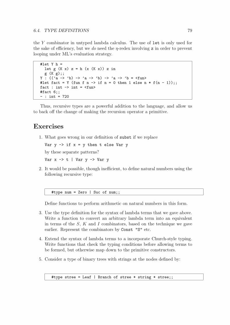
6.4. TYPE DEFINITIONS 79
the Y combinator in untyped lambda calculus. The use of let is only used forthe sake of efficiency, but we do need the η-redex involving z in order to preventlooping under ML’s evaluation strategy.
#let Y h =let g (K x) z = h (x (K x)) z ing (K g);;
Y : ((’a -> ’b) -> ’a -> ’b) -> ’a -> ’b = <fun>#let fact = Y (fun f n -> if n = 0 then 1 else n * f(n - 1));;fact : int -> int = <fun>#fact 6;;- : int = 720
Thus, recursive types are a powerful addition to the language, and allow usto back off the change of making the recursion operator a primitive.
Exercises
1. What goes wrong in our definition of subst if we replace
Var y -> if x = y then t else Var y
by these separate patterns?
Var x -> t | Var y -> Var y
2. It would be possible, though inefficient, to define natural numbers using thefollowing recursive type:
#type num = Zero | Suc of num;;
Define functions to perform arithmetic on natural numbers in this form.
3. Use the type definition for the syntax of lambda terms that we gave above.Write a function to convert an arbitrary lambda term into an equivalentin terms of the S, K and I combinators, based on the technique we gaveearlier. Represent the combinators by Const "S" etc.
4. Extend the syntax of lambda terms to a incorporate Church-style typing.Write functions that check the typing conditions before allowing terms tobe formed, but otherwise map down to the primitive constructors.
5. Consider a type of binary trees with strings at the nodes defined by:
#type stree = Leaf | Branch of stree * string * stree;;
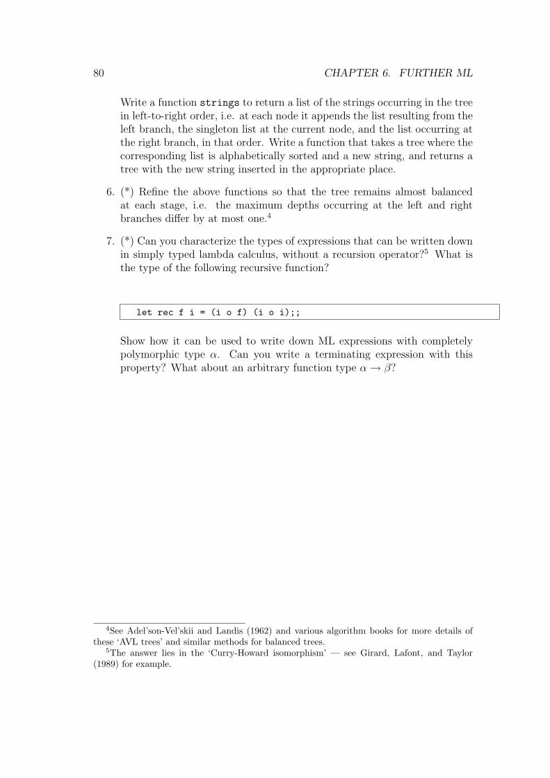
80 CHAPTER 6. FURTHER ML
Write a function strings to return a list of the strings occurring in the treein left-to-right order, i.e. at each node it appends the list resulting from theleft branch, the singleton list at the current node, and the list occurring atthe right branch, in that order. Write a function that takes a tree where thecorresponding list is alphabetically sorted and a new string, and returns atree with the new string inserted in the appropriate place.
6. (*) Refine the above functions so that the tree remains almost balancedat each stage, i.e. the maximum depths occurring at the left and rightbranches differ by at most one.4
7. (*) Can you characterize the types of expressions that can be written downin simply typed lambda calculus, without a recursion operator?5 What isthe type of the following recursive function?
let rec f i = (i o f) (i o i);;
Show how it can be used to write down ML expressions with completelypolymorphic type α. Can you write a terminating expression with thisproperty? What about an arbitrary function type α → β?
4See Adel’son-Vel’skii and Landis (1962) and various algorithm books for more details ofthese ‘AVL trees’ and similar methods for balanced trees.
5The answer lies in the ‘Curry-Howard isomorphism’ — see Girard, Lafont, and Taylor(1989) for example.

Chapter 7
Proving programs correct
As programmers know through bitter personal experience, it can be very difficultto write a program that is correct, i.e. performs its intended function. Most largeprograms have bugs. The consequences of these bugs can vary widely. Somebugs are harmless, some merely irritating. Some are deadly. For example theprograms inside heart pacemakers, aircraft autopilots, car engine managementsystems and antilock braking systems, radiation therapy machines and nuclearreactor controllers are safety critical. An error in one of them can lead directly toloss of life, possibly on a large scale. As computers become ever more pervasivein society, the number of ways in which program bugs can kill people increases.1
How can we make sure a program is correct? One very useful method is simplyto test it in a variety of situations. One tries the program out on inputs designedto exercise many different parts of it and reveal possible bugs. But usually thereare too many possible situations to try them all exhaustively, so there may stillbe bugs lying undetected. As repeatedly emphasized by various writers, notablyDijkstra, program testing can be very useful for demonstrating the presence ofbugs, but it is only in a few unusual cases where it can demonstrate their absence.
Instead of testing a program, one can try to verify it mathematically. Aprogram in a sufficiently precisely defined programming language has a definitemathematical meaning. Similarly, the requirements on a program can be ex-pressed using mathematics and logic as a precise specification. One can then tryto perform a mathematical proof that the program meets its specification.
One can contrast testing and verification of programs by considering the fol-lowing simple mathematical assertion:
ΣNn=0n =
N(N + 1)
2It is claimed that this holds for any N . We can certainly test it for any
number of particular values of N . This may lead to our intuitive confidencein the formula, such that we can hardly believe it could ever fail. However in
1Similar remarks apply to hardware, but we will focus on software.
81

82 CHAPTER 7. PROVING PROGRAMS CORRECT
general a preponderance of numerical evidence can be deceptive; there are wellknown cases in number theory where things turned out to be false against theweight of many particular cases.2 A more reliable procedure is to prove the aboveformula mathematically. This can easily be done using induction on N . In thesame way, we hope to replace testing a program on a range of inputs by somecompletely general proof that it always works correctly. It is important, however,to appreciate two limitations of program proofs.
• One has no guarantee that the execution of the program on the computercorresponds exactly to the abstract mathematical model. One must beon the lookout for discrepancies, caused perhaps by bugs in compilers andoperating systems, or physical defects in the underlying technology. This is,of course, a general problem in applications of mathematics to science. Forexample, assuming that arithmetic operations correspond exactly to theirmathematical counterparts is a natural simplifying assumption, just as onemight neglect air resistance in the analysis of a simple dynamical system.But both can be invalid in certain cases.
• The program is to be verified by proof against a mathematical specification.It is possible that this specification does not capture accurately what isactually wanted in the real world. In fact, it can be remarkably difficult toarrive at a precise mathematical version of informal requirements. There isevidence that many of the serious problems in computer systems are causednot by coding errors in the usual sense, but by a mistaken impression ofwhat is actually wanted. Just formalizing the requirements is often valuablein itself.
We can represent this situation by the following diagram:
Actual system
Mathematical model
Mathematical specification
Actual requirements
6
6
6
We are trying to establish a link between the bottom and top boxes, i.e. theactual system and the actual requirements in real life. To do this, we proceed by
2For example, Littlewood proved in 1914 that π(n) − li(n) changes sign infinitely often,where π(n) is the number of primes ≤ n and li(n) =
∫ n
0du/ln(u). This came as a surprise
since not a single sign change had been found despite extensive testing up to 1010.
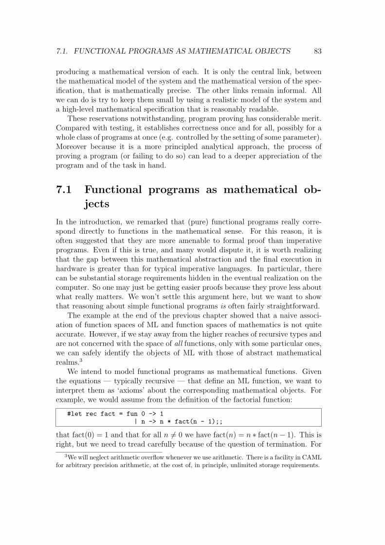
7.1. FUNCTIONAL PROGRAMS AS MATHEMATICAL OBJECTS 83
producing a mathematical version of each. It is only the central link, betweenthe mathematical model of the system and the mathematical version of the spec-ification, that is mathematically precise. The other links remain informal. Allwe can do is try to keep them small by using a realistic model of the system anda high-level mathematical specification that is reasonably readable.
These reservations notwithstanding, program proving has considerable merit.Compared with testing, it establishes correctness once and for all, possibly for awhole class of programs at once (e.g. controlled by the setting of some parameter).Moreover because it is a more principled analytical approach, the process ofproving a program (or failing to do so) can lead to a deeper appreciation of theprogram and of the task in hand.
7.1 Functional programs as mathematical ob-
jects
In the introduction, we remarked that (pure) functional programs really corre-spond directly to functions in the mathematical sense. For this reason, it isoften suggested that they are more amenable to formal proof than imperativeprograms. Even if this is true, and many would dispute it, it is worth realizingthat the gap between this mathematical abstraction and the final execution inhardware is greater than for typical imperative languages. In particular, therecan be substantial storage requirements hidden in the eventual realization on thecomputer. So one may just be getting easier proofs because they prove less aboutwhat really matters. We won’t settle this argument here, but we want to showthat reasoning about simple functional programs is often fairly straightforward.
The example at the end of the previous chapter showed that a naive associ-ation of function spaces of ML and function spaces of mathematics is not quiteaccurate. However, if we stay away from the higher reaches of recursive types andare not concerned with the space of all functions, only with some particular ones,we can safely identify the objects of ML with those of abstract mathematicalrealms.3
We intend to model functional programs as mathematical functions. Giventhe equations — typically recursive — that define an ML function, we want tointerpret them as ‘axioms’ about the corresponding mathematical objects. Forexample, we would assume from the definition of the factorial function:
#let rec fact = fun 0 -> 1| n -> n * fact(n - 1);;
that fact(0) = 1 and that for all n 6= 0 we have fact(n) = n ∗ fact(n− 1). This isright, but we need to tread carefully because of the question of termination. For
3We will neglect arithmetic overflow whenever we use arithmetic. There is a facility in CAMLfor arbitrary precision arithmetic, at the cost of, in principle, unlimited storage requirements.

84 CHAPTER 7. PROVING PROGRAMS CORRECT
negative n, the program fails to terminate, so the second equation is true onlyin the vacuous sense that both sides are ‘undefined’. It is much easier to reasonabout functions when we know they are total, so sometimes one uses a separateargument to establish termination. In the examples that follow, this is done inparallel with the correctness proof, i.e. we prove together that for each argument,the function terminates and the result satisfies our specification.
As for the actual proof that the function obeys the specification, this canbe a mathematical proof in the most general sense. However it often happensthat when functions are defined by recursion, properties of them, dually, canbe proved by induction; this includes termination. Moreover, the exact form ofinduction (arithmetical, structural, wellfounded) usually corresponds to the modeof recursion used in the definition. This should become clearer when we have seena few examples.
7.2 Exponentiation
Recall our simple definition of exponentiation:
#let rec exp x n =if n = 0 then 1else x * exp x (n - 1);;
We will prove the following property of exp:
Theorem 7.1 For all n ≥ 0 and x, exp x n is defined and exp x n = xn.Proof: The ML function exp was defined by primitive, step-by-step, recursion.It is therefore no surprise that our proof proceeds by ordinary, step-by-step induc-tion. We prove that it holds for n = 0 and then that if it holds for any n ≥ 0 italso holds for n + 1.
1. If n = 0, then by definition exp x n = 1. By definition, for any integerx, we have x0 = 1, so the desired fact is established. Note that we assume00 = 1, an example of how one must state the specification precisely — whatdoes xn mean in general? — and how it might surprise some people.
2. Suppose that for n ≥ 0 we have exp x n = xn. Since n ≥ 0, we haven + 1 6= 0 and so by definition exp x (n + 1) = x ∗ exp x ((n + 1) − 1).Therefore:
exp x (n + 1) = x ∗ exp x ((n + 1)− 1)
= x ∗ exp x n
= x ∗ xn
= xn+1

7.3. GREATEST COMMON DIVISOR 85
Q.E.D.
7.3 Greatest common divisor
Recall our function to calculate the greatest common divisor gcd(m, n) of twonatural numbers m and n:
#let rec gcd x y =if y = 0 then x else gcd y (x mod y);;
In fact, we claim this works for any integers, not just positive ones. However,one needs to understand the precise definition of gcd in that case. Let us definethe relation ‘u|v’, or ‘u divides v’ for any two integers u and v to mean ‘v is anintegral multiple of u’, i.e. there is some integer d with v = du. For example, 0|0,1|11, −2|4 but 0 6 |1, 3 6 |5. We will say that d is a greatest common divisor of xand y precisely if:
• d|x and d|y
• For any other integer d′, if d′|x and d′|y then d′|d.
Note that we say d′|d not d′ ≤ d. This belies the use of ‘greatest’, but it is infact the standard definition in algebra books. Observe that any pair of numbers(except 0 and 0) has two gcds, since if d is a gcd of x and y, so is −d.
Our specification is now: for any integers x and y, d = gcd x y is a gcd ofx and y. This is another good example of how providing a precise specification,even for such a simple function, is harder than it looks. This specification alsoexemplifies the common property that it does not completely specify the answer,merely places certain constraints on it. If we defined:
#let rec ngcd x y = -(gcd x y);;
then the function ngcd would satisfy the specification just as well as gcd. Ofcourse, we are free to tighten the specification if we wish, e.g. insist that if x andy are positive, so is the gcd returned.
The gcd function is not defined simply by primitive recursion. In fact, gcdx y is defined in terms of gcd y (x mod y) in the step case. Correspondingly,we do not use step-by-step induction, but wellfounded induction. We want awellfounded relation that decreases over recursive calls; this will guarantee ter-mination and act as a handle for proofs by wellfounded induction. In general,complicated relations on the arguments are required. But often it is easy toconcoct a measure that maps the arguments to natural numbers such that themeasure decreases over recursive calls. Such is the case here: the measure is |y|.
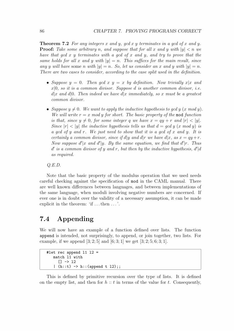
86 CHAPTER 7. PROVING PROGRAMS CORRECT
Theorem 7.2 For any integers x and y, gcd x y terminates in a gcd of x and y.Proof: Take some arbitrary n, and suppose that for all x and y with |y| < n wehave that gcd x y terminates with a gcd of x and y, and try to prove that thesame holds for all x and y with |y| = n. This suffices for the main result, sinceany y will have some n with |y| = n. So, let us consider an x and y with |y| = n.There are two cases to consider, according to the case split used in the definition.
• Suppose y = 0. Then gcd x y = x by definition. Now trivially x|x andx|0, so it is a common divisor. Suppose d is another common divisor, i.e.d|x and d|0. Then indeed we have d|x immediately, so x must be a greatestcommon divisor.
• Suppose y 6= 0. We want to apply the inductive hypothesis to gcd y (x mod y).We will write r = x mod y for short. The basic property of the mod functionis that, since y 6= 0, for some integer q we have x = qy + r and |r| < |y|.Since |r| < |y| the inductive hypothesis tells us that d = gcd y (x mod y) isa gcd of y and r. We just need to show that it is a gcd of x and y. It iscertainly a common divisor, since if d|y and d|r we have d|x, as x = qy+r.Now suppose d′|x and d′|y. By the same equation, we find that d′|r. Thusd′ is a common divisor of y and r, but then by the inductive hypothesis, d′|das required.
Q.E.D.
Note that the basic property of the modulus operation that we used needscareful checking against the specification of mod in the CAML manual. Thereare well known differences between languages, and between implementations ofthe same language, when moduli involving negative numbers are concerned. Ifever one is in doubt over the validity of a necessary assumption, it can be madeexplicit in the theorem: ‘if . . . then . . . ’.
7.4 Appending
We will now have an example of a function defined over lists. The functionappend is intended, not surprisingly, to append, or join together, two lists. Forexample, if we append [3; 2; 5] and [6; 3; 1] we get [3; 2; 5; 6; 3; 1].
#let rec append l1 l2 =match l1 with[] -> l2
| (h::t) -> h::(append t l2);;
This is defined by primitive recursion over the type of lists. It is definedon the empty list, and then for h :: t in terms of the value for t. Consequently,
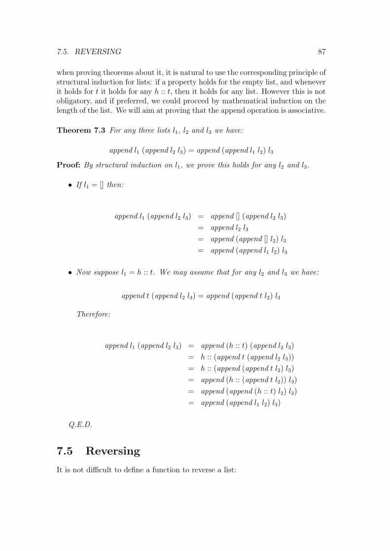
7.5. REVERSING 87
when proving theorems about it, it is natural to use the corresponding principle ofstructural induction for lists: if a property holds for the empty list, and wheneverit holds for t it holds for any h :: t, then it holds for any list. However this is notobligatory, and if preferred, we could proceed by mathematical induction on thelength of the list. We will aim at proving that the append operation is associative.
Theorem 7.3 For any three lists l1, l2 and l3 we have:
append l1 (append l2 l3) = append (append l1 l2) l3
Proof: By structural induction on l1, we prove this holds for any l2 and l3.
• If l1 = [] then:
append l1 (append l2 l3) = append [] (append l2 l3)
= append l2 l3
= append (append [] l2) l3
= append (append l1 l2) l3
• Now suppose l1 = h :: t. We may assume that for any l2 and l3 we have:
append t (append l2 l3) = append (append t l2) l3
Therefore:
append l1 (append l2 l3) = append (h :: t) (append l2 l3)
= h :: (append t (append l2 l3))
= h :: (append (append t l2) l3)
= append (h :: (append t l2)) l3)
= append (append (h :: t) l2) l3)
= append (append l1 l2) l3)
Q.E.D.
7.5 Reversing
It is not difficult to define a function to reverse a list:
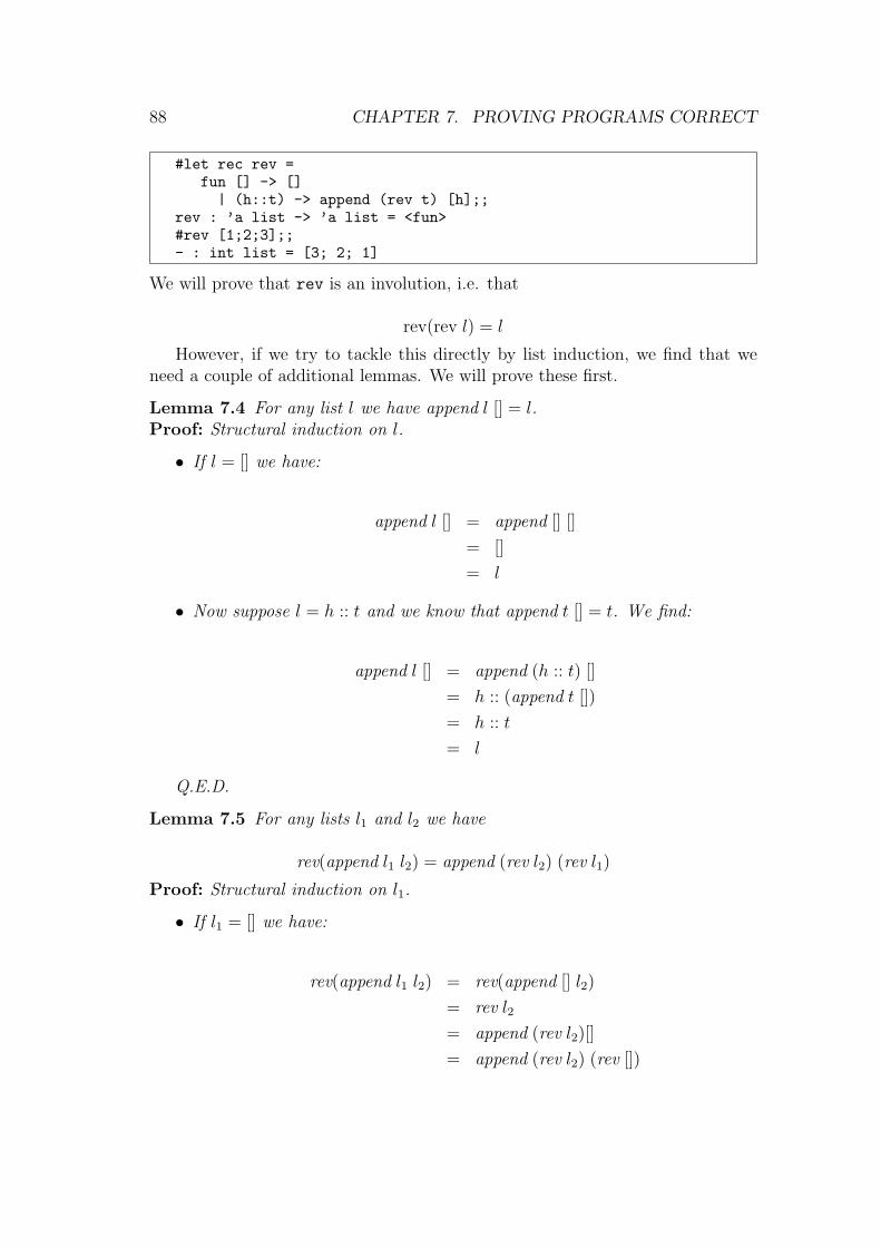
88 CHAPTER 7. PROVING PROGRAMS CORRECT
#let rec rev =fun [] -> []| (h::t) -> append (rev t) [h];;
rev : ’a list -> ’a list = <fun>#rev [1;2;3];;- : int list = [3; 2; 1]
We will prove that rev is an involution, i.e. that
rev(rev l) = l
However, if we try to tackle this directly by list induction, we find that weneed a couple of additional lemmas. We will prove these first.
Lemma 7.4 For any list l we have append l [] = l.Proof: Structural induction on l.
• If l = [] we have:
append l [] = append [] []
= []
= l
• Now suppose l = h :: t and we know that append t [] = t. We find:
append l [] = append (h :: t) []
= h :: (append t [])
= h :: t
= l
Q.E.D.
Lemma 7.5 For any lists l1 and l2 we have
rev(append l1 l2) = append (rev l2) (rev l1)
Proof: Structural induction on l1.
• If l1 = [] we have:
rev(append l1 l2) = rev(append [] l2)
= rev l2
= append (rev l2)[]
= append (rev l2) (rev [])
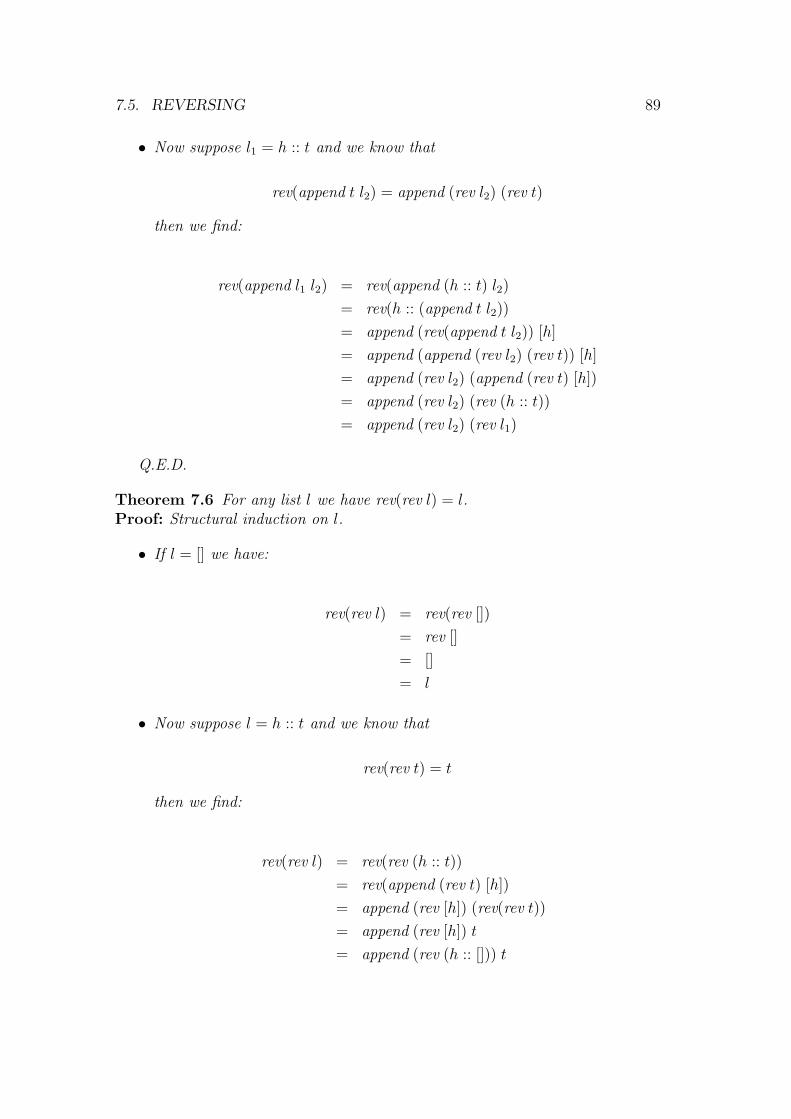
7.5. REVERSING 89
• Now suppose l1 = h :: t and we know that
rev(append t l2) = append (rev l2) (rev t)
then we find:
rev(append l1 l2) = rev(append (h :: t) l2)
= rev(h :: (append t l2))
= append (rev(append t l2)) [h]
= append (append (rev l2) (rev t)) [h]
= append (rev l2) (append (rev t) [h])
= append (rev l2) (rev (h :: t))
= append (rev l2) (rev l1)
Q.E.D.
Theorem 7.6 For any list l we have rev(rev l) = l.Proof: Structural induction on l.
• If l = [] we have:
rev(rev l) = rev(rev [])
= rev []
= []
= l
• Now suppose l = h :: t and we know that
rev(rev t) = t
then we find:
rev(rev l) = rev(rev (h :: t))
= rev(append (rev t) [h])
= append (rev [h]) (rev(rev t))
= append (rev [h]) t
= append (rev (h :: [])) t

90 CHAPTER 7. PROVING PROGRAMS CORRECT
= append (append (rev []) [h]) t
= append (append [] [h]) t
= append [h] t
= append (h :: []) t
= h :: (append [] t)
= h :: t
= l
Q.E.D.
There are lots of theorems relating the list operations that can be proved ina similar style. Generally, one proceeds by list induction. In subtler cases, onehas to split off lemmas which are themselves proved inductively, and sometimesto generalize the theorem before proceeding by induction. There are plenty ofexamples in the exercises for readers to try their hand at.
Further reading
Neumann (1995) catalogues the dangers arising from the use of computers insociety, including those arising from software bugs. A very readable discussionof the issues, with extensive discussion of some interesting examples, is given byPeterson (1996). The general issue of software verification was at one time con-troversial, with DeMillo, Lipton, and Perlis (1979) among others arguing againstit. A cogent discussion is given by Barwise (1989). There is now a large liter-ature in software verification, though much of it is concerned with imperativeprograms. Many introductory functional programming books such as Paulson(1991) and Reade (1989) give some basic examples like the ones here. It is alsoworth looking at the work of Boyer and Moore (1979) on verifying properties ofpure LISP functions expressed inside their theorem prover. One of the largestreal proofs of the type we consider here is the verification by Aagaard and Leeser(1994) of a boolean simplifier used in VLSI logic synthesis.
Exercises
1. Prove the correctness of the more efficient program we gave for performingexponentiation:

7.5. REVERSING 91
#let square x = x * x;;#let rec exp x n =if n = 0 then 1else if n mod 2 = 0 then square(exp x (n / 2))else x * square(exp x (n / 2));;
2. Recall the definition of length:
#let rec length =fun [] -> 0| (h::t) -> 1 + length t;;
Prove that length(rev l) = length l and that length(append l1 l2) =length l1 + length l2.
3. Define the map function, which applies a function to each element of a list,as follows:
#let rec map f =fun [] -> []| (h::t) -> (f h)::(map f t);;
Prove that if l 6= [] then hd(map f l) = f(hd l), and that map f (rev l) =rev (map f l). Recall the definition of function composition:
#let o f g = fun x -> f(g x);;#infix "o";;
Prove that map f (map g l) = map (f ◦ g) l.
4. McCarthy’s ‘91 function’ can be defined by:
#let rec f x = if x > 100 then x - 10else f(f(x + 11));;
Prove that for n ≤ 101, we have f(n) = 91. Pay careful attention toestablishing termination. (Hint: a possible measure is 101− x.)
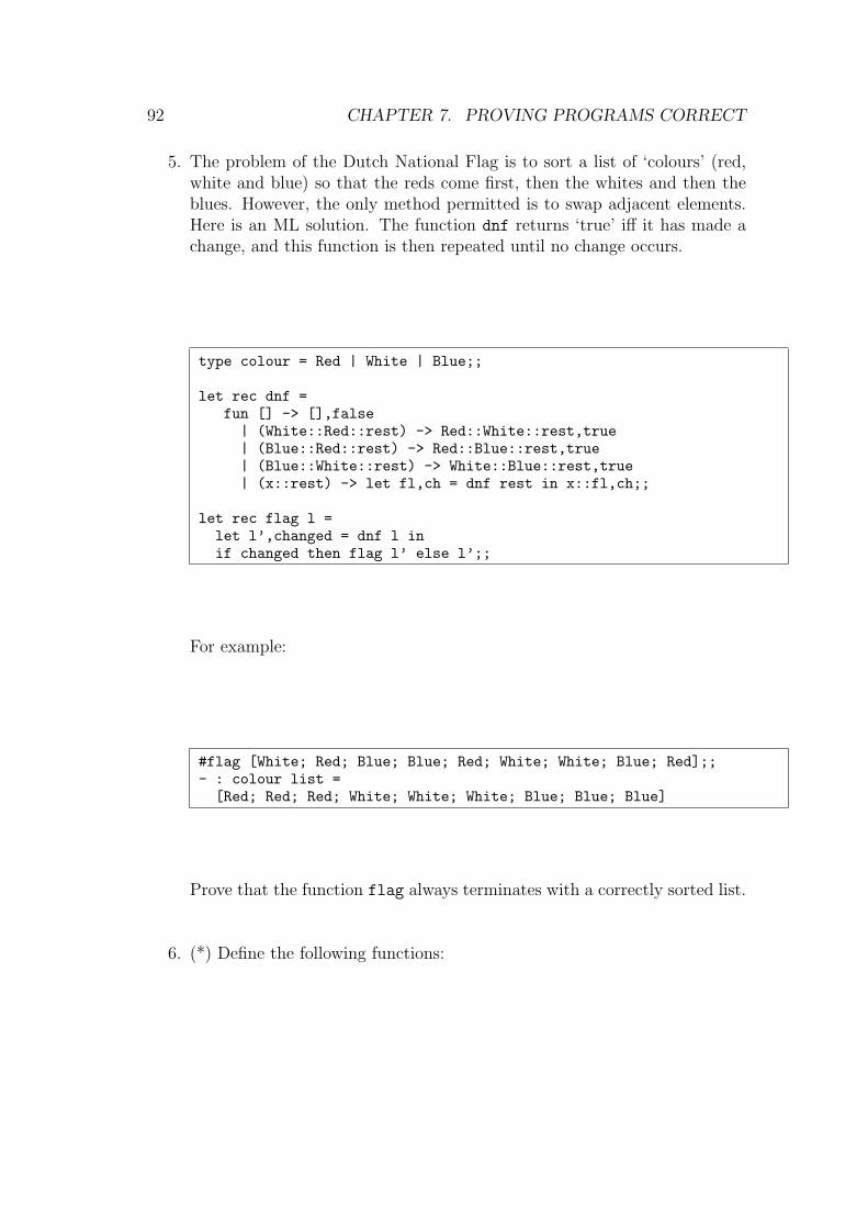
92 CHAPTER 7. PROVING PROGRAMS CORRECT
5. The problem of the Dutch National Flag is to sort a list of ‘colours’ (red,white and blue) so that the reds come first, then the whites and then theblues. However, the only method permitted is to swap adjacent elements.Here is an ML solution. The function dnf returns ‘true’ iff it has made achange, and this function is then repeated until no change occurs.
type colour = Red | White | Blue;;
let rec dnf =fun [] -> [],false| (White::Red::rest) -> Red::White::rest,true| (Blue::Red::rest) -> Red::Blue::rest,true| (Blue::White::rest) -> White::Blue::rest,true| (x::rest) -> let fl,ch = dnf rest in x::fl,ch;;
let rec flag l =let l’,changed = dnf l inif changed then flag l’ else l’;;
For example:
#flag [White; Red; Blue; Blue; Red; White; White; Blue; Red];;- : colour list =[Red; Red; Red; White; White; White; Blue; Blue; Blue]
Prove that the function flag always terminates with a correctly sorted list.
6. (*) Define the following functions:
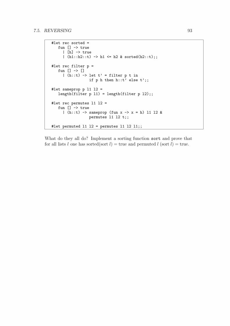
7.5. REVERSING 93
#let rec sorted =fun [] -> true| [h] -> true| (h1::h2::t) -> h1 <= h2 & sorted(h2::t);;
#let rec filter p =fun [] -> []| (h::t) -> let t’ = filter p t in
if p h then h::t’ else t’;;
#let sameprop p l1 l2 =length(filter p l1) = length(filter p l2);;
#let rec permutes l1 l2 =fun [] -> true| (h::t) -> sameprop (fun x -> x = h) l1 l2 &
permutes l1 l2 t;;
#let permuted l1 l2 = permutes l1 l2 l1;;
What do they all do? Implement a sorting function sort and prove thatfor all lists l one has sorted(sort l) = true and permuted l (sort l) = true.

Chapter 8
Effective ML
In this chapter, we discuss some of the techniques and tricks that ML program-mers can use to make programs more elegant and more efficient. We then go onto discuss some additional imperative features that can be used when the purelyfunctional style seems inappropriate.
8.1 Useful combinators
The flexibility of higher order functions often means that one can write some veryuseful little functions that can be re-used for a variety of related tasks. These areoften called combinators, and not simply because they can be regarded as lambdaterms with no free variables. It often turns out that these functions are so flexiblethat practically anything can be implemented by plugging them together, ratherthan, say, explicitly making a recursive definition. In this way they correspond tothe original view of combinators as ubiquitous building blocks for mathematicalexpressions.
For example, a very useful combinator for list operations, often called ‘itlist’or ‘fold’, performs the following operation:
itlist f [x1; x2; . . . ; xn] b = f x1 (f x2 (f x3 (· · · (f xn b))))
A straightforward definition in ML is:
#let rec itlist f =fun [] b -> b| (h::t) b -> f h (itlist f t b);;
itlist : (’a -> ’b -> ’b) -> ’a list -> ’b -> ’b = <fun>
Quite commonly, when defining a recursive function over lists, all one is doingis repeatedly applying some operator in this manner. By using itlist withthe appropriate argument, one can implement such functions very easily withoutexplicit use of recursion. A typical use is a function to add all the elements of alist of numbers:
94

8.1. USEFUL COMBINATORS 95
#let sum l = itlist (fun x sum -> x + sum) l 0;;sum : int list -> int = <fun>#sum [1;2;3;4;5];;- : int = 15#sum [];;- : int = 0#sum [1;1;1;1];;- : int = 4
Those especially keen on brevity might prefer to code sum as:
#let sum l = itlist (prefix +) l 0;;
It is easy to modify this function to form a product rather than a sum:
#let prod l = itlist (prefix *) l 1;;
Many useful list operations can be implemented in this way. For example hereis a function to filter out only those elements of a list satisfying a predicate:
#let filter p l = itlist (fun x s -> if p x then x::s else s) l [];;filter : (’a -> bool) -> ’a list -> ’a list = <fun>#filter (fun x -> x mod 2 = 0) [1;6;4;9;5;7;3;2];;- : int list = [6; 4; 2]
Here are functions to find whether either all or some of the elements of a listsatisfy a predicate:
#let forall p l = itlist (fun h a -> p(h) & a) l true;;forall : (’a -> bool) -> ’a list -> bool = <fun>#let exists p l = itlist (fun h a -> p(h) or a) l false;;exists : (’a -> bool) -> ’a list -> bool = <fun>#forall (fun x -> x < 3) [1;2];;- : bool = true#forall (fun x -> x < 3) [1;2;3];;- : bool = false
and here are alternative versions of old favourites length, append and map:
#let length l = itlist (fun x s -> s + 1) l 0;;length : ’a list -> int = <fun>#let append l m = itlist (fun h t -> h::t) l m;;append : ’a list -> ’a list -> ’a list = <fun>#let map f l = itlist (fun x s -> (f x)::s) l [];;map : (’a -> ’b) -> ’a list -> ’b list = <fun>
Some of these functions can themselves become useful combinators, and so onupwards. For example, if we are interested in treating lists as sets, i.e. avoidingduplicate elements, then many of the standard set operations can be expressedvery simply in terms of the combinators above:

96 CHAPTER 8. EFFECTIVE ML
#let mem x l = exists (fun y -> y = x) l;;mem : ’a -> ’a list -> bool = <fun>#let insert x l =if mem x l then l else x::l;;
insert : ’a -> ’a list -> ’a list = <fun>#let union l1 l2 = itlist insert l1 l2;;union : ’a list -> ’a list -> ’a list = <fun>#let setify l = union l [];;setify : ’a list -> ’a list = <fun>#let Union l = itlist union l [];;Union : ’a list list -> ’a list = <fun>#let intersect l1 l2 = filter (fun x -> mem x l2) l1;;intersect : ’a list -> ’a list -> ’a list = <fun>#let subtract l1 l2 = filter (fun x -> not mem x l2) l1;;subtract : ’a list -> ’a list -> ’a list = <fun>#let subset l1 l2 = forall (fun t -> mem t l2) l1;;subset : ’a list -> ’a list -> bool = <fun>
The setify function is supposed to turn a list into a set by eliminating anyduplicate elements.
8.2 Writing efficient code
Here we accumulate some common tricks of the trade, which can often make MLprograms substantially more efficient. In order to justify some of them, we needto sketch in general terms how certain constructs are executed in hardware.
8.2.1 Tail recursion and accumulators
The principal control mechanism in functional programs is recursion. If we areinterested in efficient programs, it behoves us to think a little about how recursionis implemented on conventional hardware. In fact, there is not, in this respectat least, much difference between the implementation of ML and many otherlanguages with dynamic variables, such as C.
If functions cannot be called recursively, then we are safe in storing their localvariables (which includes the values of arguments) at a fixed place in memory— this is what FORTRAN does. However, this is not possible in general if thefunction can be called recursively. A call to a function f with one set of argumentsmay include within it a call to f with a different set of arguments. The old oneswould be overwritten, even if the outer version of f needs to refer to them againafter the inner call has finished. For example, consider the factorial function yetagain:
#let rec fact n = if n = 0 then 1else n * fact(n - 1);;
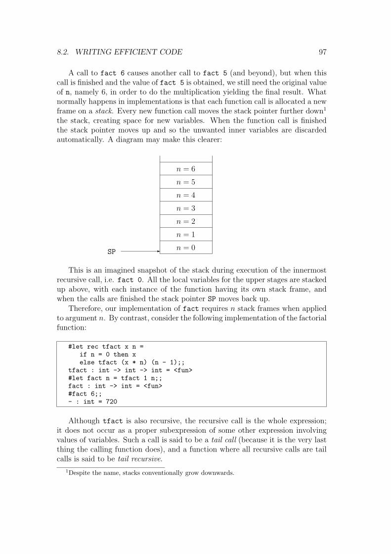
8.2. WRITING EFFICIENT CODE 97
A call to fact 6 causes another call to fact 5 (and beyond), but when thiscall is finished and the value of fact 5 is obtained, we still need the original valueof n, namely 6, in order to do the multiplication yielding the final result. Whatnormally happens in implementations is that each function call is allocated a newframe on a stack. Every new function call moves the stack pointer further down1
the stack, creating space for new variables. When the function call is finishedthe stack pointer moves up and so the unwanted inner variables are discardedautomatically. A diagram may make this clearer:
SP - n = 0
n = 1
n = 2
n = 3
n = 4
n = 5
n = 6
This is an imagined snapshot of the stack during execution of the innermostrecursive call, i.e. fact 0. All the local variables for the upper stages are stackedup above, with each instance of the function having its own stack frame, andwhen the calls are finished the stack pointer SP moves back up.
Therefore, our implementation of fact requires n stack frames when appliedto argument n. By contrast, consider the following implementation of the factorialfunction:
#let rec tfact x n =if n = 0 then xelse tfact (x * n) (n - 1);;
tfact : int -> int -> int = <fun>#let fact n = tfact 1 n;;fact : int -> int = <fun>#fact 6;;- : int = 720
Although tfact is also recursive, the recursive call is the whole expression;it does not occur as a proper subexpression of some other expression involvingvalues of variables. Such a call is said to be a tail call (because it is the very lastthing the calling function does), and a function where all recursive calls are tailcalls is said to be tail recursive.
1Despite the name, stacks conventionally grow downwards.

98 CHAPTER 8. EFFECTIVE ML
What is significant about tail calls? When making a recursive call to tfact,there is no need to preserve the old values of the local variables. Exactly the same,fixed, area of storage can be used. This of course depends on the compiler’s beingintelligent enough to recognize the fact, but most compilers, including CAMLLight, are. Consequently, re-coding a function so that the recursive core of it istail recursive can dramatically cut down the use of storage. For functions like thefactorial, it is hardly likely that they will be called with large enough values ofn to make the stack overflow. However the naive implementations of many listfunctions can cause such an effect when the argument lists are long.
The additional argument x of the tfact function is called an accumulator,because it accumulates the result as the recursive calls rack up, and is thenreturned at the end. Working in this way, rather than modifying the return valueon the way back up, is a common way of making functions tail recursive.
We have remarked that a fixed area of storage can be used for the argumentsto a tail recursive function. On this view, one can look at a tail recursive functionas a thinly-veiled imperative implementation. There is an obvious parallel withour C implementation of the factorial as an iterative function:
int fact(int n)
{ int x = 1;
while (n > 0)
{ x = x * n;
n = n - 1;
}
return x;
}
The initialization x = 1 corresponds to our setting of x to 1 by an outerwrapper function fact. The central while loop corresponds to the recursivecalls, the only difference being that the arguments to the tail recursive functionmake explicit that part of the state we are interested in assigning to. Ratherthan assigning and looping, we make a recursive call with the variables updated.Using similar tricks and making the state explicit, one can easily write essentiallyimperative code in an ostensibly functional style, with the knowledge that understandard compiler optimizations, the effect inside the machine will, in fact, bemuch the same.
8.2.2 Minimizing consing
We have already considered the use of stack space. But various constructs infunctional programs use another kind of store, usually allocated from an areacalled the heap. Whereas the stack grows and shrinks in a sequential mannerbased on the flow of control between functions, other storage used by the ML
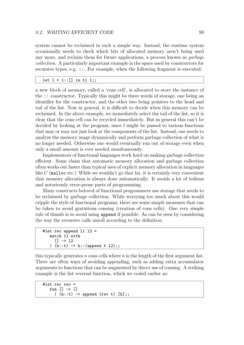
8.2. WRITING EFFICIENT CODE 99
system cannot be reclaimed in such a simple way. Instead, the runtime systemoccasionally needs to check which bits of allocated memory aren’t being usedany more, and reclaim them for future applications, a process known as garbagecollection. A particularly important example is the space used by constructors forrecursive types, e.g. ::. For example, when the following fragment is executed:
let l = 1::[] in tl l;;
a new block of memory, called a ‘cons cell’, is allocated to store the instance ofthe :: constructor. Typically this might be three words of storage, one being anidentifier for the constructor, and the other two being pointers to the head andtail of the list. Now in general, it is difficult to decide when this memory can bereclaimed. In the above example, we immediately select the tail of the list, so it isclear that the cons cell can be recycled immediately. But in general this can’t bedecided by looking at the program, since l might be passed to various functionsthat may or may not just look at the components of the list. Instead, one needs toanalyze the memory usage dynamically and perform garbage collection of what isno longer needed. Otherwise one would eventually run out of storage even whenonly a small amount is ever needed simultaneously.
Implementors of functional languages work hard on making garbage collectionefficient. Some claim that automatic memory allocation and garbage collectionoften works out faster than typical uses of explicit memory allocation in languageslike C (malloc etc.) While we wouldn’t go that far, it is certainly very convenientthat memory allocation is always done automatically. It avoids a lot of tediousand notoriously error-prone parts of programming.
Many constructs beloved of functional programmers use storage that needs tobe reclaimed by garbage collection. While worrying too much about this wouldcripple the style of functional programs, there are some simple measures that canbe taken to avoid gratuitous consing (creation of cons cells). One very simplerule of thumb is to avoid using append if possible. As can be seen by consideringthe way the recursive calls unroll according to the definition
#let rec append l1 l2 =match l1 with[] -> l2
| (h::t) -> h::(append t l2);;
this typically generates n cons cells where n is the length of the first argument list.There are often ways of avoiding appending, such as adding extra accumulatorarguments to functions that can be augmented by direct use of consing. A strikingexample is the list reversal function, which we coded earlier as:
#let rec rev =fun [] -> []| (h::t) -> append (rev t) [h];;

100 CHAPTER 8. EFFECTIVE ML
This typically generates about n2/2 cons cells, where n is the length of thelist. The following alternative, using an accumulator, only generates n of them:
#let rev =let rec reverse acc =fun [] -> acc| (h::t) -> reverse (h::acc) t in
reverse [];;
Moreover, the recursive core reverse is tail recursive, so we also save stackspace, and win twice over.
For another typical situation where we can avoid appending by judicious useof accumulators, consider the problem of returning the fringe of a binary tree, i.e.a list of the leaves in left-to-right order. If we define the type of binary trees as:
#type btree = Leaf of string| Branch of btree * btree;;
then a simple coding is the following
#let rec fringe =fun (Leaf s) -> [s]| (Branch(l,r)) -> append (fringe l) (fringe r);;
However the following more refined version performs fewer conses:
#let fringe =let rec fr t acc =match t with(Leaf s) -> s::acc
| (Branch(l,r)) -> fr l (fr r acc) infun t -> fr t [];;
Note that we have written the accumulator as the second argument, so thatthe recursive call has a more natural left-to-right reading. Here is a simple ex-ample of how either version of fringe may be used:
#fringe (Branch(Branch(Leaf "a",Leaf "b"),Branch(Leaf "c",Leaf "d")));;
- : string list = ["a"; "b"; "c"; "d"]
The first version creates 6 cons cells, the second only 4. On larger trees theeffect can be more dramatic. Another situation where gratuitous consing cancrop up is in pattern matching. For example, consider the code fragment:
fun [] -> []| (h::t) -> if h < 0 then t else h::t;;

8.2. WRITING EFFICIENT CODE 101
The ‘else’ arm creates a cons cell even though what it constructs was in factthe argument to the function. That is, it is taking the argument apart and thenrebuilding it. One simple way of avoiding this is to recode the function as:
fun l ->match l with[] -> []
| (h::t) -> if h < 0 then t else l;;
However ML offers a more flexible alternative: using the as keyword, a namemay be identified with certain components of the pattern, so that it never needsto be rebuilt. For example:
fun [] -> []| (h::t as l) -> if h < 0 then t else l;;
8.2.3 Forcing evaluation
We have emphasized that, since ML does not evaluate underneath lambdas, onecan use lambdas to delay evaluation. We will see some interesting exampleslater. Conversely, however, it can happen that one wants to force evaluation ofexpressions that are hidden underneath lambdas. For example, recall the tailrecursive factorial above:
#let rec tfact x n =if n = 0 then xelse tfact (x * n) (n - 1);;
#let fact n = tfact 1 n;;
Since we never really want to use tfact directly, it seems a pity to bind it toa name. Instead, we can make it local to the factorial function:
#let fact1 n =let rec tfact x n =if n = 0 then xelse tfact (x * n) (n - 1) in
tfact 1 n;;
This, however, has the defect that the local recursive definition is only eval-uated after fact1 receives its argument, since before that it is hidden under alambda. Moreover, it is then reevaluated each time fact is called. We can changethis as follows
#let fact2 =let rec tfact x n =if n = 0 then xelse tfact (x * n) (n - 1) in
tfact 1;;
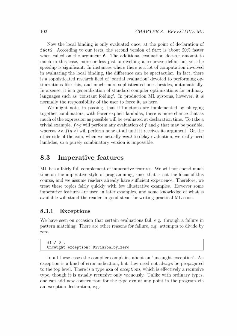
102 CHAPTER 8. EFFECTIVE ML
Now the local binding is only evaluated once, at the point of declaration offact2. According to our tests, the second version of fact is about 20% fasterwhen called on the argument 6. The additional evaluation doesn’t amount tomuch in this case, more or less just unravelling a recursive definition, yet thespeedup is significant. In instances where there is a lot of computation involvedin evaluating the local binding, the difference can be spectacular. In fact, thereis a sophisticated research field of ‘partial evaluation’ devoted to performing op-timizations like this, and much more sophisticated ones besides, automatically.In a sense, it is a generalization of standard compiler optimizations for ordinarylanguages such as ‘constant folding’. In production ML systems, however, it isnormally the responsibility of the user to force it, as here.
We might note, in passing, that if functions are implemented by pluggingtogether combinators, with fewer explicit lambdas, there is more chance that asmuch of the expression as possible will be evaluated at declaration time. To take atrivial example, f ◦g will perform any evaluation of f and g that may be possible,whereas λx. f(g x) will perform none at all until it receives its argument. On theother side of the coin, when we actually want to delay evaluation, we really needlambdas, so a purely combinatory version is impossible.
8.3 Imperative features
ML has a fairly full complement of imperative features. We will not spend muchtime on the imperative style of programming, since that is not the focus of thiscourse, and we assume readers already have sufficient experience. Therefore, wetreat these topics fairly quickly with few illustrative examples. However someimperative features are used in later examples, and some knowledge of what isavailable will stand the reader in good stead for writing practical ML code.
8.3.1 Exceptions
We have seen on occasion that certain evaluations fail, e.g. through a failure inpattern matching. There are other reasons for failure, e.g. attempts to divide byzero.
#1 / 0;;Uncaught exception: Division_by_zero
In all these cases the compiler complains about an ‘uncaught exception’. Anexception is a kind of error indication, but they need not always be propagatedto the top level. There is a type exn of exceptions, which is effectively a recursivetype, though it is usually recursive only vacuously. Unlike with ordinary types,one can add new constructors for the type exn at any point in the program viaan exception declaration, e.g.
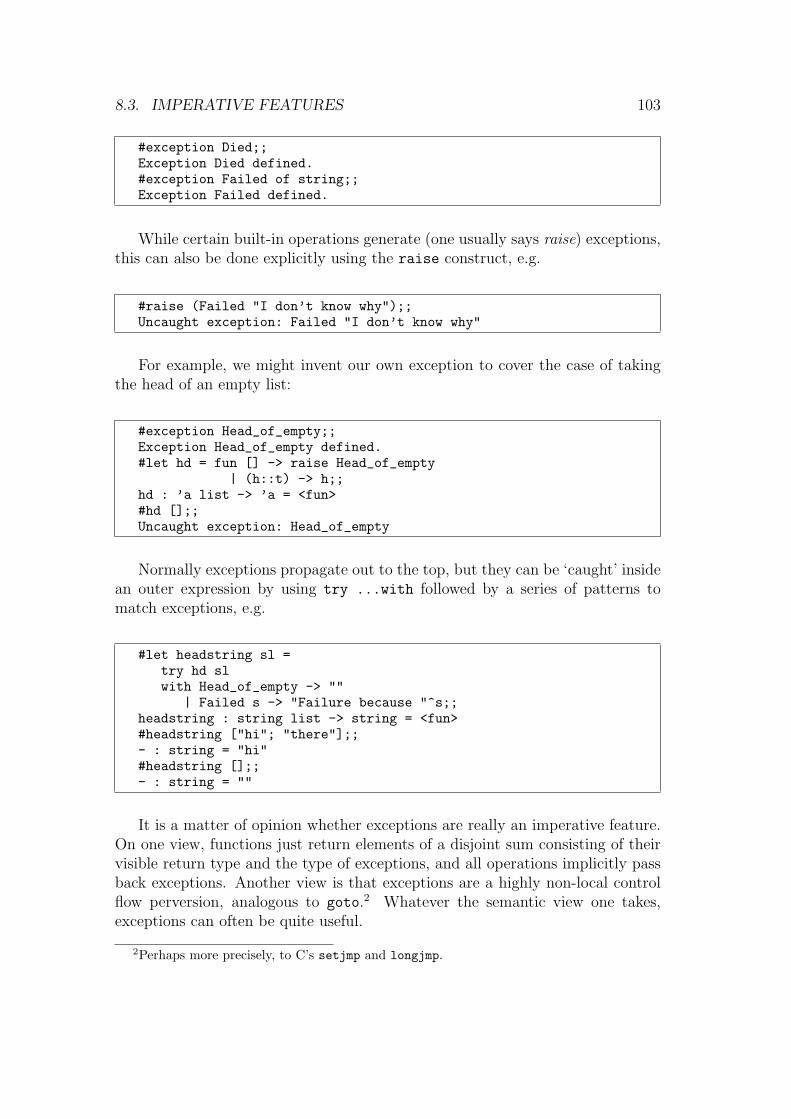
8.3. IMPERATIVE FEATURES 103
#exception Died;;Exception Died defined.#exception Failed of string;;Exception Failed defined.
While certain built-in operations generate (one usually says raise) exceptions,this can also be done explicitly using the raise construct, e.g.
#raise (Failed "I don’t know why");;Uncaught exception: Failed "I don’t know why"
For example, we might invent our own exception to cover the case of takingthe head of an empty list:
#exception Head_of_empty;;Exception Head_of_empty defined.#let hd = fun [] -> raise Head_of_empty
| (h::t) -> h;;hd : ’a list -> ’a = <fun>#hd [];;Uncaught exception: Head_of_empty
Normally exceptions propagate out to the top, but they can be ‘caught’ insidean outer expression by using try ...with followed by a series of patterns tomatch exceptions, e.g.
#let headstring sl =try hd slwith Head_of_empty -> ""
| Failed s -> "Failure because "^s;;headstring : string list -> string = <fun>#headstring ["hi"; "there"];;- : string = "hi"#headstring [];;- : string = ""
It is a matter of opinion whether exceptions are really an imperative feature.On one view, functions just return elements of a disjoint sum consisting of theirvisible return type and the type of exceptions, and all operations implicitly passback exceptions. Another view is that exceptions are a highly non-local controlflow perversion, analogous to goto.2 Whatever the semantic view one takes,exceptions can often be quite useful.
2Perhaps more precisely, to C’s setjmp and longjmp.

104 CHAPTER 8. EFFECTIVE ML
8.3.2 References and arrays
ML does have real assignable variables, and expressions can, as a side-effect,modify the values of these variables. They are explicitly accessed via references(pointers in C parlance) and the references themselves behave more like ordinaryML values. Actually this approach is quite common in C too. For example, if onewants so-called ‘variable parameters’ in C, where changes to the local variablespropagate outside, the only way to do it is to pass a pointer, so that the functioncan dereference it. Similar techniques are often used where the function is to passback composite data.
In ML, one sets up a new assignable memory cell with the initial contents x bywriting ref x. (Initialization is compulsory.) This expression yields a reference(pointer) to the cell. Subsequent access to the contents of the cell requires anexplicit dereference using the ! operator, similar to unary * in C. The cell isassigned to using a conventional-looking assignment statement. For example:
#let x = ref 1;;x : int ref = ref 1#!x;;- : int = 1#x := 2;;- : unit = ()#!x;;- : int = 2#x := !x + !x;;- : unit = ()#x;;- : int ref = ref 4#!x;;- : int = 4
Note that in most respects ref behaves like a type constructor, so one canpattern-match against it. Thus one could actually define an indirection operatorlike !:
#let contents_of (ref x) = x;;contents_of : ’a ref -> ’a = <fun>#contents_of x;;- : int = 4
As well as being mutable, references are sometimes useful for creating ex-plicitly shared data structures. One can easily create graph structures wherenumerous nodes contain a pointer to some single subgraph.
Apart from single cells, one can also use arrays in ML. In CAML these arecalled vectors. An array of elements of type α has type α vect. A fresh vectorof size n, with each element initialized to x — once again the initialization iscompulsory — is created using the following call:

8.3. IMPERATIVE FEATURES 105
#make_vect n x;;
One can then read element m of a vector v using:
#vect_item v m;;
and write value y to element m of v using:
#vect_assign v m y;;
These operations correspond to the expressions v[m] and v[m] = y in C. Theelements of an array are numbered from zero. For example:
#let v = make_vect 5 0;;v : int vect = [|0; 0; 0; 0; 0|]#vect_item v 1;;- : int = 0#vect_assign v 1 10;;- : unit = ()#v;;- : int vect = [|0; 10; 0; 0; 0|]#vect_item v 1;;- : int = 10
All reading and writing is constrained by bounds checking, e.g.
#vect_item v 5;;Uncaught exception: Invalid_argument "vect_item"
8.3.3 Sequencing
There is no need for an explicit sequencing operation in ML, since the normalrules of evaluation allow one to impose an order. For example one can do:
#let _ = x := !x + 1 inlet _ = x := !x + 1 inlet _ = x := !x + 1 inlet _ = x := !x + 1 in();;
and the expressions are evaluated in the expected order. Here we use a specialpattern which throws away the value, but we could use a dummy variable nameinstead. Nevertheless, it is more attractive to use the conventional notation forsequencing, and this is possible in ML by using a single semicolon:
#x := !x + 1;x := !x + 1;x := !x + 1;x := !x + 1;;

106 CHAPTER 8. EFFECTIVE ML
8.3.4 Interaction with the type system
While polymorphism works very well for the pure functional core of ML, it hasunfortunate interactions with some imperative features. For example, considerthe following:
#let l = ref [];;
Then l would seem to have polymorphic type α list ref . In accordance withthe usual rules of let-polymorphism we should be able to use it with two differenttypes, e.g. first
#l := [1];;
and then
#hd(!l) = true;;
But this isn’t reasonable, because we would actually be writing something asan object of type int then reading it as an object of type bool. Consequently,some restriction on the usual rule of let polymorphism is called for where ref-erences are concerned. There have been many attempts to arrive at a soundbut convenient restriction of the ML type system, some of them very compli-cated. Recently, different versions of ML seem to be converging on a relativelysimple method, called the value restriction, due to Wright (1996), and CAMLimplements this restriction, with a twist regarding toplevel bindings. Indeed, theabove sequence fails. But the intermediate behaviour is interesting. If we look atthe first line we see:
#let l = ref [];;l : ’_a list ref = ref []
The underscore on the type variable indicates that l is not polymorphic inthe usual sense; rather, it has a single fixed type, although that type is as yetundetermined. The second line works fine:
#l := [1];;- : unit = ()
but if we now look at the type of l, we see that:
#l;;- : int list ref = ref [1]
The pseudo-polymorphic type has now been fixed. Granted this, it is clearthat the last line must fail:

8.3. IMPERATIVE FEATURES 107
#hd(!l) = true;;Toplevel input:>hd(!l) = true;;> ^^^^This expression has type bool,but is used with type int.
So far, this seems quite reasonable, but we haven’t yet explained why the sameunderscored type variables oocur in apparently quite innocent purely functionalexpressions, and why, moreover, they often disappear on eta-expansion, e.g.
#let I x = x;;I : ’a -> ’a = <fun>#I o I;;it : ’_a -> ’_a = <fun>#let I2 = I o I in fun x -> I2 x;;- : ’_a -> ’_a = <fun>#fun x -> (I o I) x;;it : ’a -> ’a = <fun>
Other techniques for polymorphic references often rely on encoding in thetypes the fact that an expression may involve references. This seems natural,but it can lead to the types of functions becoming cluttered with this specialinformation. It is unattractive that the particular implementation of the function,e.g. imperative or functional, should be reflected in its type.
Wright’s solution, on the other hand, uses just the basic syntax of the ex-pression being let-bound, insisting that it is a so-called value before generalizingthe type. What is really wanted is knowledge of whether the expression maycause side-effects when evaluated. However since this is undecidable in general,the simple syntactic criterion of its being or not being a value is used. Roughlyspeaking, an expression is a value if it admits no further evaluation accordingto the ML rules — this is why an expression can often be made into a valueby performing a reverse eta conversion. Unfortunately this works against thetechniques for forcing evaluation.
Exercises
1. Define the C combinator as:
#let C f x y = f y x;;
What does the following function do?
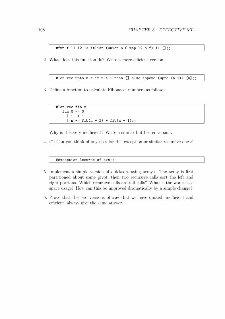
108 CHAPTER 8. EFFECTIVE ML
#fun f l1 l2 -> itlist (union o C map l2 o f) l1 [];;
2. What does this function do? Write a more efficient version.
#let rec upto n = if n < 1 then [] else append (upto (n-1)) [n];;
3. Define a function to calculate Fibonacci numbers as follows:
#let rec fib =fun 0 -> 0| 1 -> 1| n -> fib(n - 2) + fib(n - 1);;
Why is this very inefficient? Write a similar but better version.
4. (*) Can you think of any uses for this exception or similar recursive ones?
#exception Recurse of exn;;
5. Implement a simple version of quicksort using arrays. The array is firstpartitioned about some pivot, then two recursive calls sort the left andright portions. Which recursive calls are tail calls? What is the worst-casespace usage? How can this be improved dramatically by a simple change?
6. Prove that the two versions of rev that we have quoted, inefficient andefficient, always give the same answer.
Chapter 9
Examples
As we have said, ML was originally designed as a metalanguage for a computertheorem prover. However it is suitable for plenty of other applications, mostlyfrom the same general field of ‘symbolic computation’. In this chapter we will givesome examples of characteristic uses of ML. It is not necessary that the readershould understand every detail of the particular examples, e.g. the analyses ofreal number approximations given below. However it is worth trying out theseprograms and similar examples for yourself, and doing some of the exercises.There is no better way of getting a feel for how ML is actually used.
9.1 Symbolic differentiation
The phrase ‘symbolic computation’ is a bit vague, but roughly speaking it coversapplications where manipulation of mathematical expressions, in general con-taining variables, is emphasized at the expense of actual numerical calculation.There are several successful ‘computer algebra systems’ such as Axiom, Mapleand Mathematica, which can do certain symbolic operations that are useful inmathematics, e.g. factorizing polynomials and differentiating and integrating ex-pressions. (They are also capable of purely numerical work.) We will illustratehow this sort of application can be tackled using ML.
We use symbolic differentiation as our example, because there is an algorithmto do it which is fairly simple and well known. The reader is probably familiarwith certain derivatives of basic operations, e.g d
dxsin(x) = cos(x), as well as
results such as the Chain Rule and Product Rule for calculating the derivativesof composite expressions in terms of the derivatives of the components. Justas one can use these systematically in order to find derivatives, it is possible toprogram a fairly straightforward algorithm to do it in ML.
109
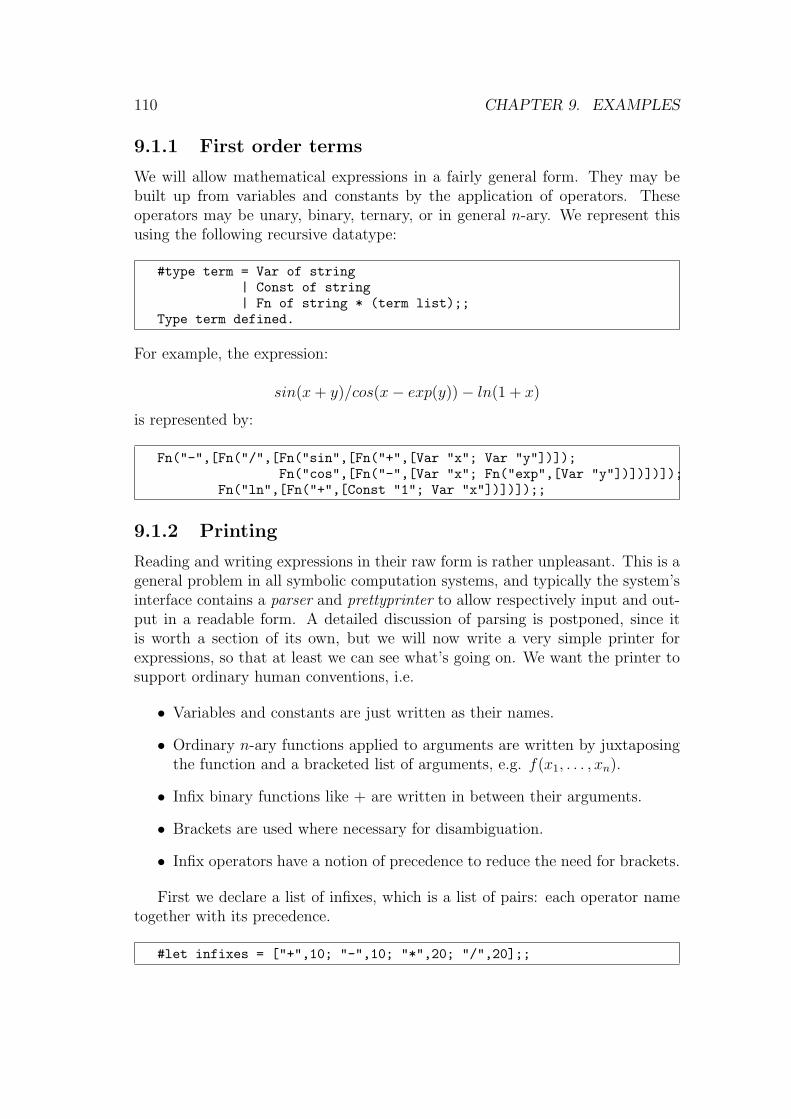
110 CHAPTER 9. EXAMPLES
9.1.1 First order terms
We will allow mathematical expressions in a fairly general form. They may bebuilt up from variables and constants by the application of operators. Theseoperators may be unary, binary, ternary, or in general n-ary. We represent thisusing the following recursive datatype:
#type term = Var of string| Const of string| Fn of string * (term list);;
Type term defined.
For example, the expression:
sin(x + y)/cos(x− exp(y))− ln(1 + x)
is represented by:
Fn("-",[Fn("/",[Fn("sin",[Fn("+",[Var "x"; Var "y"])]);Fn("cos",[Fn("-",[Var "x"; Fn("exp",[Var "y"])])])]);
Fn("ln",[Fn("+",[Const "1"; Var "x"])])]);;
9.1.2 Printing
Reading and writing expressions in their raw form is rather unpleasant. This is ageneral problem in all symbolic computation systems, and typically the system’sinterface contains a parser and prettyprinter to allow respectively input and out-put in a readable form. A detailed discussion of parsing is postponed, since itis worth a section of its own, but we will now write a very simple printer forexpressions, so that at least we can see what’s going on. We want the printer tosupport ordinary human conventions, i.e.
• Variables and constants are just written as their names.
• Ordinary n-ary functions applied to arguments are written by juxtaposingthe function and a bracketed list of arguments, e.g. f(x1, . . . , xn).
• Infix binary functions like + are written in between their arguments.
• Brackets are used where necessary for disambiguation.
• Infix operators have a notion of precedence to reduce the need for brackets.
First we declare a list of infixes, which is a list of pairs: each operator nametogether with its precedence.
#let infixes = ["+",10; "-",10; "*",20; "/",20];;

9.1. SYMBOLIC DIFFERENTIATION 111
It is common to use lists in this way to represent finite partial functions, sinceit allows more flexibility. They are commonly called association lists, and arevery common in functional programming.1 In order to convert the list into apartial function we use assoc:
#let rec assoc a ((x,y)::rest) = if a = x then y else assoc a rest;;Toplevel input:>let rec assoc a ((x,y)::rest) = if a = x then y else assoc a rest;;> ^^^^^^^^^^^^^^^^^^^^^^^^^^^^^^^^^^^^^^^^^^^^^^^^^^^^^^^^^Warning: this matching is not exhaustive.assoc : ’a -> (’a * ’b) list -> ’b = <fun>
The compiler warns us that if the appropriate data is not found in the list,the function will fail. Now we can define a function to get the infix precedenceof a function:
#let get_precedence s = assoc s infixes;;get_precedence : string -> int = <fun>#get_precedence "+";;- : int = 10#get_precedence "/";;- : int = 20#get_precedence "%";;Uncaught exception: Match_failure ("", 6544, 6601)
Note that if we ever change this list of infixes, then any functions such asget precedence that use it need to be redeclared. This is the main reason whymany LISP programmers prefer dynamic binding. However we can make the setof infixes arbitrarily extensible by making it into a reference and dereferencing iton each application:
#let infixes = ref ["+",10; "-",10; "*",20; "/",20];;infixes : (string * int) list ref =ref ["+", 10; "-", 10; "*", 20; "/", 20]
#let get_precedence s = assoc s (!infixes);;get_precedence : string -> int = <fun>#get_precedence "^";;Uncaught exception: Match_failure ("", 6544, 6601)#infixes := ("^",30)::(!infixes);;- : unit = ()#get_precedence "^";;- : int = 30
1For more heavyweight applications, some alternative such as hash tables is much better,but for simple applications where the lists don’t get too long, this kind of linear list is simpleand adequate.

112 CHAPTER 9. EXAMPLES
Note that by the ML evaluation rules, the dereferencing is only applied afterthe function get precedence receives its argument, and hence results in theset of infixes at that time. We can also define a function to decide whether afunction has any data associated with it. One way is simply to try the functionget precedence and see if it works:
#let is_infix s =try get_precedence s; truewith _ -> false;;
An alternative is to use a general function can that finds out whether anotherfunction succeeds:
#let can f x = try f x; true with _ -> false;;can : (’a -> ’b) -> ’a -> bool = <fun>#let is_infix = can get_precedence;;is_infix : string -> bool = <fun>
We will use the following functions that we have already considered:
#let hd(h::t) = h;;#let tl(h::t) = t;;#let rec length l = if l = [] then 0 else 1 + length(tl l);;
Without further ado, here is a function to convert a term into a string.
#let rec string_of_term prec =fun (Var s) -> s| (Const c) -> c| (Fn(f,args)) ->
if length args = 2 & is_infix f thenlet prec’ = get_precedence f inlet s1 = string_of_term prec’ (hd args)and s2 = string_of_term prec’ (hd(tl args)) inlet ss = s1^" "^f^" "^s2 inif prec’ <= prec then "("^ss^")" else ss
elsef^"("^(string_of_terms args)^")"
and string_of_terms t =match t with
[] -> ""| [t] -> string_of_term 0 t| (h::t) -> (string_of_term 0 h)^","^(string_of_terms t);;
The first argument prec indicates the precedence level of the operator of whichthe currently considered expression is an immediate subterm. Now if the currentexpression has an infix binary operator at the top level, parentheses are needed
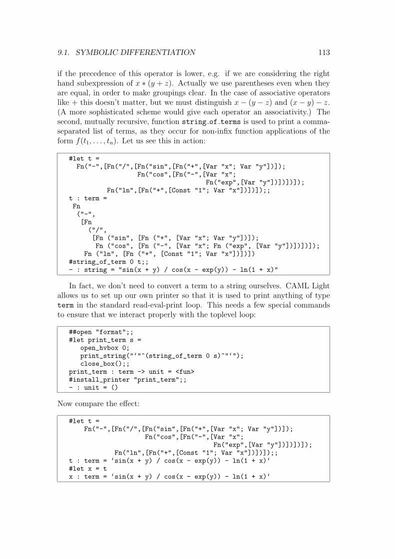
9.1. SYMBOLIC DIFFERENTIATION 113
if the precedence of this operator is lower, e.g. if we are considering the righthand subexpression of x ∗ (y + z). Actually we use parentheses even when theyare equal, in order to make groupings clear. In the case of associative operatorslike + this doesn’t matter, but we must distinguish x− (y − z) and (x− y)− z.(A more sophisticated scheme would give each operator an associativity.) Thesecond, mutually recursive, function string of terms is used to print a comma-separated list of terms, as they occur for non-infix function applications of theform f(t1, . . . , tn). Let us see this in action:
#let t =Fn("-",[Fn("/",[Fn("sin",[Fn("+",[Var "x"; Var "y"])]);
Fn("cos",[Fn("-",[Var "x";Fn("exp",[Var "y"])])])]);
Fn("ln",[Fn("+",[Const "1"; Var "x"])])]);;t : term =Fn("-",[Fn("/",[Fn ("sin", [Fn ("+", [Var "x"; Var "y"])]);Fn ("cos", [Fn ("-", [Var "x"; Fn ("exp", [Var "y"])])])]);
Fn ("ln", [Fn ("+", [Const "1"; Var "x"])])])#string_of_term 0 t;;- : string = "sin(x + y) / cos(x - exp(y)) - ln(1 + x)"
In fact, we don’t need to convert a term to a string ourselves. CAML Lightallows us to set up our own printer so that it is used to print anything of typeterm in the standard read-eval-print loop. This needs a few special commandsto ensure that we interact properly with the toplevel loop:
##open "format";;#let print_term s =
open_hvbox 0;print_string("‘"^(string_of_term 0 s)^"‘");close_box();;
print_term : term -> unit = <fun>#install_printer "print_term";;- : unit = ()
Now compare the effect:
#let t =Fn("-",[Fn("/",[Fn("sin",[Fn("+",[Var "x"; Var "y"])]);
Fn("cos",[Fn("-",[Var "x";Fn("exp",[Var "y"])])])]);
Fn("ln",[Fn("+",[Const "1"; Var "x"])])]);;t : term = ‘sin(x + y) / cos(x - exp(y)) - ln(1 + x)‘#let x = tx : term = ‘sin(x + y) / cos(x - exp(y)) - ln(1 + x)‘

114 CHAPTER 9. EXAMPLES
Once the new printer is installed, it is used whenever CAML wants to printsomething of type term, even if it is a composite datastructure such as a pair:
#(x,t);;- : term * term =‘sin(x + y) / cos(x - exp(y)) - ln(1 + x)‘,‘sin(x + y) / cos(x - exp(y)) - ln(1 + x)‘
or a list:
#[x; t; x];;- : term list =[‘sin(x + y) / cos(x - exp(y)) - ln(1 + x)‘;‘sin(x + y) / cos(x - exp(y)) - ln(1 + x)‘;‘sin(x + y) / cos(x - exp(y)) - ln(1 + x)‘]
This printer is rather crude in that it will not break up large expressionsintelligently across lines. The CAML library format, from which we used a fewfunctions above, provides for a better approach. Instead of converting the terminto a string then printing it in one piece, we can make separate printing calls fordifferent parts of it, and intersperse these with some special function calls thathelp the printing mechanism to understand where to break the lines. Many ofthe principles used in this and similar ‘prettyprinting engines’ are due to Oppen(1980). We will not consider this in detail here — see the CAML manual fordetails.2
9.1.3 Derivatives
Now it is a fairly simple matter to define the derivative function. First let usrecall the systematic method we are taught in school:
• If the expression is one of the standard functions applied to an argumentthat is the variable of differentiation, e.g. sin(x), return the known deriva-tive.
• If the expression is of the form f(x) + g(x) then apply the rule for sums,returning f ′(x) + g′(x). Likewise for subtraction etc.
• If the expression is of the form f(x) ∗ g(x) then apply the product rule, i.e.return f ′(x) ∗ g(x) + f(x) ∗ g′(x).
• If the expression is one of the standard functions applied to a compositeargument, say f(g(x)) then apply the Chain Rule and so give g′(x)∗f ′(g(x))
2There is also a tutorial, written by Pierre Weis, available online as part of the CAML page:‘http://pauillac.inria.fr/caml/FAQ/format-eng.html’.

9.1. SYMBOLIC DIFFERENTIATION 115
This is nothing but a recursive algorithm, though that terminology is seldomused in schools. We can program it in ML very directly:
#let rec differentiate x tm = match tm withVar y -> if y = x then Const "1" else Const "0"
| Const c -> Const "0"| Fn("-",[t]) -> Fn("-",[differentiate x t])| Fn("+",[t1;t2]) -> Fn("+",[differentiate x t1;
differentiate x t2])| Fn("-",[t1;t2]) -> Fn("-",[differentiate x t1;
differentiate x t2])| Fn("*",[t1;t2]) ->
Fn("+",[Fn("*",[differentiate x t1; t2]);Fn("*",[t1; differentiate x t2])])
| Fn("inv",[t]) -> chain x t(Fn("-",[Fn("inv",[Fn("^",[t;Const "2"])])]))
| Fn("^",[t;n]) -> chain x t(Fn("*",[n; Fn("^",[t; Fn("-",[n; Const "1"])])]))
| Fn("exp",[t]) -> chain x t tm| Fn("ln",[t]) -> chain x t (Fn("inv",[t]))| Fn("sin",[t]) -> chain x t (Fn("cos",[t]))| Fn("cos",[t]) -> chain x t
(Fn("-",[Fn("sin",[t])]))| Fn("/",[t1;t2]) -> differentiate x
(Fn("*",[t1; Fn("inv",[t2])]))| Fn("tan",[t]) -> differentiate x
(Fn("/",[Fn("sin",[t]); Fn("cos",[t])]))and chain x t u = Fn("*",[differentiate x t; u]);;
The chain function just avoids repeating the chain rule construction for manyoperations. Apart from that, we just systematically apply rules for sums, prod-ucts etc. and the known derivatives of standard functions. Of course, we couldadd other functions such as the hyperbolic functions and inverse trigonometricfunctions if desired. A couple of cases, namely division and tan, avoid a compli-cated definition by applying the differentiator to an alternative formulation.
9.1.4 Simplification
If we try the differentiator out on our running example, then it works quite well:

116 CHAPTER 9. EXAMPLES
#t;;- : term = ‘sin(x + y) / cos(x - exp(y)) - ln(1 + x)‘#differentiate "x" t;;- : term =‘(((1 + 0) * cos(x + y)) * inv(cos(x - exp(y))) +sin(x + y) * (((1 - 0 * exp(y)) * -(sin(x - exp(y)))) *-(inv(cos(x - exp(y)) ^ 2)))) - (0 + 1) * inv(1 + x)‘
#differentiate "y" t;;- : term =‘(((0 + 1) * cos(x + y)) * inv(cos(x - exp(y))) +sin(x + y) * (((0 - 1 * exp(y)) * -(sin(x - exp(y)))) *-(inv(cos(x - exp(y)) ^ 2)))) - (0 + 0) * inv(1 + x)‘
#differentiate "z" t;;- : term =‘(((0 + 0) * cos(x + y)) * inv(cos(x - exp(y))) +sin(x + y) * (((0 - 0 * exp(y)) * -(sin(x - exp(y)))) *-(inv(cos(x - exp(y)) ^ 2)))) - (0 + 0) * inv(1 + x)‘
However, it fails to make various obvious simplifications such as 0 ∗ x = 0and x + 0 = x. Some of these redundant expressions are created by the ratherunsubtle differentiation strategy which, for instance, applies the chain rule to f(t)even where t is just the variable of differentiation. However, some would be hardto avoid without making the differentiator much more complicated. Accordingly,let us define a separate simplification function that gets rid of some of theseunnecessary expressions.
#let simp =fun (Fn("+",[Const "0"; t])) -> t| (Fn("+",[t; Const "0"])) -> t| (Fn("-",[t; Const "0"])) -> t| (Fn("-",[Const "0"; t])) -> Fn("-",[t])| (Fn("+",[t1; Fn("-",[t2])])) -> Fn("-",[t1; t2])| (Fn("*",[Const "0"; t])) -> Const "0"| (Fn("*",[t; Const "0"])) -> Const "0"| (Fn("*",[Const "1"; t])) -> t| (Fn("*",[t; Const "1"])) -> t| (Fn("*",[Fn("-",[t1]); Fn("-",[t2])])) -> Fn("*",[t1; t2])| (Fn("*",[Fn("-",[t1]); t2])) -> Fn("-",[Fn("*",[t1; t2])])| (Fn("*",[t1; Fn("-",[t2])])) -> Fn("-",[Fn("*",[t1; t2])])| (Fn("-",[Fn("-",[t])])) -> t| t -> t;;
This just applies the simplification at the top level of the term. We need toexecute it in a bottom-up sweep. This will also bring negations upwards throughproducts. In some cases it would be more efficient to simplify in a top-downsweep, e.g. 0 ∗ t for a complicated expression t, but this would need repeatingfor terms like (0 + 0) ∗ 2. The choice is rather like that between normal andapplicative order reduction in lambda calculus.

9.1. SYMBOLIC DIFFERENTIATION 117
#let rec dsimp =fun (Fn(fn,args)) -> simp(Fn(fn,map dsimp args))| t -> simp t;;
Now we get better results:
#dsimp(differentiate "x" t);;- : term =‘(cos(x + y) * inv(cos(x - exp(y))) +sin(x + y) * (sin(x - exp(y)) *inv(cos(x - exp(y)) ^ 2))) - inv(1 + x)‘
#dsimp(differentiate "y" t);;- : term =‘cos(x + y) * inv(cos(x - exp(y))) -sin(x + y) * ((exp(y) * sin(x - exp(y))) *inv(cos(x - exp(y)) ^ 2))‘
#dsimp(differentiate "z" t);;- : term = ‘0‘
In general, one can always add more and more sophisticated simplification.For example, consider:
#let t2 = Fn("tan",[Var "x"]);;t2 : term = ‘tan(x)‘#differentiate "x" t2;;- : term =‘(1 * cos(x)) * inv(cos(x)) +sin(x) * ((1 * -(sin(x))) * -(inv(cos(x) ^ 2)))‘
#dsimp(differentiate "x" t2);;- : term = ‘cos(x) * inv(cos(x)) +
sin(x) * (sin(x) * inv(cos(x) ^ 2))‘
We would like to simplify cos(x) * inv(cos(x)) simply to 1, ignoring, asmost commercial computer algebra systems do, the possibility that cos(x) mightbe zero. We can certainly add new clauses to the simplifier for that. Similarly,we might like to collect up terms in the second summand. However here we startto see that human psychology plays a role. Which of the following is preferable?It is hard for the machine to decide unaided.
sin(x) * (sin(x) * inv(cos(x) ^ 2))
sin(x) ^ 2 * inv(cos(x) ^ 2)
sin(x) ^ 2 / cos(x) ^ 2
(sin(x) / cos(x)) ^ 2
tan(x) ^ 2

118 CHAPTER 9. EXAMPLES
And having chosen the last one, should it then convert
1 + tan(x) ^ 2
into
sec(x) ^ 2
Certainly, it is shorter and more conventional. However it relies on the factthat we know the definitions of these fairly obscure trig functions like sec. What-ever the machine decides to do, it is likely that some user will find it upsetting.
9.2 Parsing
A defect of our previous example was that the input had to be written explicitlyin terms of type constructors. Here we will show how to write a parser for thissituation, and make our code sufficiently general that it can easily be appliedto similar formal languages. Generally speaking, the problem of parsing is asfollows. A formal language is defined by a grammar, which is a set of productionrules for each syntactic category. For a language of terms with two infix operators+ and * and only alphanumeric variables and numeral (0, 1 etc.) constants, itmight look like this:
term −→ name(termlist)
| name
| (term)
| numeral
| -term
| term + term
| term * term
termlist −→ term,termlist
| term
We will assume for the moment that we know what names and numeralsare, but we could have similar rules defining them in terms of single characters.Now this set of production rules gives us a way of generating the concrete, linearrepresentation for all terms. Note that name, numeral, term and termlist aremeant to be variables in the above, whereas elements like ‘+’ and ‘(’ written inbold type are actual characters. For example we have:

9.2. PARSING 119
term −→ term * term
−→ term * (term)
−→ term * (term + term)
−→ term * (term + term * term)
−→ numeral * (name + name * name)
so, following similar rules for name and numeral, we can generate for example:
10 * (x + y * z)
The task of parsing is to reverse this process of applying production rules, i.e.to take a string and discover how it could have been generated by the productionrules for a syntactic category. Typically, the output is a parse tree, i.e. a treestructure that shows clearly the sequence of applications of the rules.
One problem with parsing is that the grammar may be ambiguous, i.e. a givenstring can often be generated in several different ways. This is the case in ourexample above, for the string could also have been generated by:
term −→ term * term
−→ term * (term)
−→ term * (term * term)
−→ term * (term + term * term)
−→ numeral * (name + name * name)
The obvious way to fix this is to specify rules of precedence and associativityfor infix operators. However, we can make the grammar unambiguous withoutintroducing additional mechanisms at the cost of adding new syntactic categories:
atom −→ name(termlist)
| name
| numeral
| (term)
| -atom
mulexp −→ atom * mulexp
| atom
term −→ mulexp + term
| mulexp
termlist −→ term,termlist
| term

120 CHAPTER 9. EXAMPLES
Note that this makes both infix operators right associative. For a more com-plicated example of this technique in action, look at the formal definition ofexpressions in the ANSI C Standard.
9.2.1 Recursive descent parsing
The production rules suggest a very simple way of going about parsing using aseries of mutually recursive functions. The idea is to have a function for eachsyntactic category, and a recursive structure that reflects exactly the mutual re-cursion found in the grammar itself. For example, the procedure for parsingterms, say term will, on encountering a - symbol, make a recursive call to itselfto parse the subterm, and on encountering a name followed by an opening paren-thesis, will make a recursive call to termlist. This in itself will make at leastone recursive call to term, and so on. Such a style of programming is particularlynatural in a language like ML where recursion is the principal control mechanism.
In our ML implementation, we suppose that we have some input list of objectsof arbitrary type α for the parser to consume. These might simply be characters,but in fact there is usually a separate level of lexical analysis which collectscharacters together into tokens such as ‘x12’, ‘:=’ and ‘96’, so by the time wereach this level the input is a list of tokens. We avoid committing ourselvesto any particular type. Similarly, we will allow the parser to construct objectsof arbitrary type β from its input. These might for example be parse trees asmembers of a recursive datatype, or might simply be numbers if the parser is totake an expression and evaluate it. Now in general, a parser might not consumeall its input, so we also make it output the remaining tokens. Therefore, a parserwill have type
(α)list → β × (α)list
For example, when given the input characters (x + y) * z the function atom
should process the characters (x + y) and leave the remaining characters * z. Itmight return a parse tree for the processed expression using our earlier recursivetype, and hence we would have:
atom "(x + y) * z" = Fn("+",[Var "x"; Var "y"]),"* z"
Since any call of the function atom must be from within the function mulexp,this second function will use the result of atom and deal with the input thatremains, making a second call to atom to process the expression ‘z’.
9.2.2 Parser combinators
Another reason why this technique works particularly well in ML is that we candefine some useful combinators for plugging parsers together. In fact, by giving

9.2. PARSING 121
them infix status, we can make the ML parser program look quite similar instructure to the original grammar defining the language.
First we declare an exception to be used where parsing fails. Then we definean infix ++ that applies two parsers in sequence, pairing up their results, and andinfix || which tries first one parser, then the other. We then define a many-foldversion of ++ that repeats a parser as far as possible, putting the results into alist. Finally, the infix >> is used to modify the results of a parser according to afunction.
The CAML rules for symbolic identifiers such as ++ make them infix automat-ically, so we suppress this during the definition using the prefix keyword. Theirprecedences are also automatic, following from the usual precedence of their firstcharacters as arithmetic operations etc. That is, ++ is the strongest, >> falls inthe middle, and || is the weakest; this is exactly what we want.
exception Noparse;;
let prefix || parser1 parser2 input =try parser1 inputwith Noparse -> parser2 input;;
let prefix ++ parser1 parser2 input =let result1,rest1 = parser1 input inlet result2,rest2 = parser2 rest1 in(result1,result2),rest2;;
let rec many parser input =try let result,next = parser input in
let results,rest = many parser next in(result::results),rest
with Noparse -> [],input;;
let prefix >> parser treatment input =let result,rest = parser input intreatment(result),rest;;
We will, in what follows, use the following other functions. Most of these havebeen defined above, the main exception being explode which converts a stringinto a list of 1-elements strings. It uses the inbuilt functions sub_string andstring_length; we do not describe them in detail but their function should beeasy to grasp from the example.
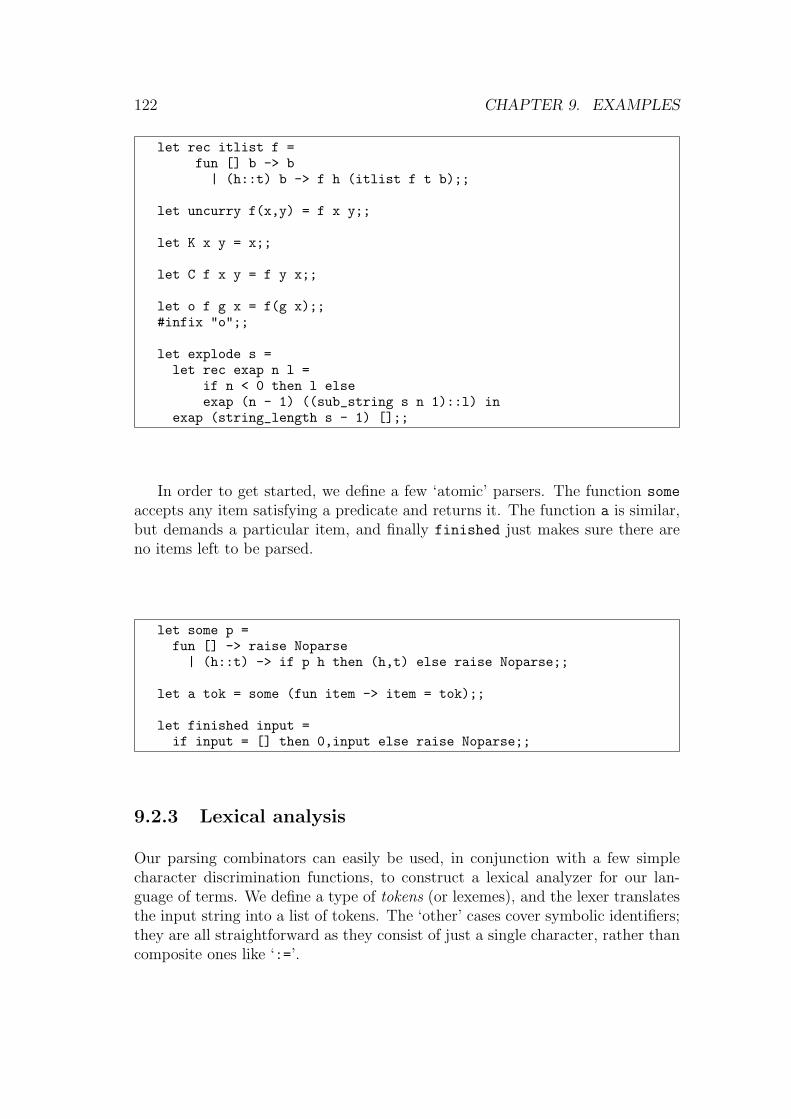
122 CHAPTER 9. EXAMPLES
let rec itlist f =fun [] b -> b| (h::t) b -> f h (itlist f t b);;
let uncurry f(x,y) = f x y;;
let K x y = x;;
let C f x y = f y x;;
let o f g x = f(g x);;#infix "o";;
let explode s =let rec exap n l =
if n < 0 then l elseexap (n - 1) ((sub_string s n 1)::l) in
exap (string_length s - 1) [];;
In order to get started, we define a few ‘atomic’ parsers. The function some
accepts any item satisfying a predicate and returns it. The function a is similar,but demands a particular item, and finally finished just makes sure there areno items left to be parsed.
let some p =fun [] -> raise Noparse| (h::t) -> if p h then (h,t) else raise Noparse;;
let a tok = some (fun item -> item = tok);;
let finished input =if input = [] then 0,input else raise Noparse;;
9.2.3 Lexical analysis
Our parsing combinators can easily be used, in conjunction with a few simplecharacter discrimination functions, to construct a lexical analyzer for our lan-guage of terms. We define a type of tokens (or lexemes), and the lexer translatesthe input string into a list of tokens. The ‘other’ cases cover symbolic identifiers;they are all straightforward as they consist of just a single character, rather thancomposite ones like ‘:=’.

9.2. PARSING 123
type token = Name of string | Num of string | Other of string;;
let lex =let several p = many (some p) inlet lowercase_letter s = "a" <= s & s <= "z" inlet uppercase_letter s = "A" <= s & s <= "Z" inlet letter s = lowercase_letter s or uppercase_letter s inlet alpha s = letter s or s = "_" or s = "’" inlet digit s = "0" <= s & s <= "9" inlet alphanum s = alpha s or digit s inlet space s = s = " " or s = "\n" or s = "\t" inlet collect(h,t) = h^(itlist (prefix ^) t "") inlet rawname =
some alpha ++ several alphanum >> (Name o collect) inlet rawnumeral =
some digit ++ several digit >> (Num o collect) inlet rawother = some (K true) >> Other inlet token =(rawname || rawnumeral || rawother) ++ several space >> fst in
let tokens = (several space ++ many token) >> snd inlet alltokens = (tokens ++ finished) >> fst infst o alltokens o explode;;
For example:
#lex "sin(x + y) * cos(2 * x + y)";;- : token list =[Name "sin"; Other "("; Name "x"; Other "+"; Name "y"; Other ")";Other "*"; Name "cos"; Other "("; Num "2"; Other "*"; Name "x";Other "+"; Name "y"; Other ")"]
9.2.4 Parsing terms
Since we are now working at the level of tokens, we define trivial parsers to accepttokens of (only) a certain kind:
let name =fun (Name s::rest) -> s,rest| _ -> raise Noparse;;
let numeral =fun (Num s::rest) -> s,rest| _ -> raise Noparse;;
let other =fun (Other s::rest) -> s,rest| _ -> raise Noparse;;
Now we can define a parser for terms, in a form very similar to the originalgrammar. The main difference is that each production rule has associated withit some sort of special action to take as a result of parsing.

124 CHAPTER 9. EXAMPLES
let rec atom input= (name ++ a (Other "(") ++ termlist ++ a (Other ")")
>> (fun (((name,_),args),_) -> Fn(name,args))|| name
>> (fun s -> Var s)|| numeral
>> (fun s -> Const s)|| a (Other "(") ++ term ++ a (Other ")")
>> (snd o fst)|| a (Other "-") ++ atom
>> snd) inputand mulexp input
= (atom ++ a(Other "*") ++ mulexp>> (fun ((a,_),m) -> Fn("*",[a;m]))
|| atom) inputand term input
= (mulexp ++ a(Other "+") ++ term>> (fun ((a,_),m) -> Fn("+",[a;m]))
|| mulexp) inputand termlist input
= (term ++ a (Other ",") ++ termlist>> (fun ((h,_),t) -> h::t)
|| term>> (fun h -> [h])) input;;
Let us package everything up as a single parsing function:
let parser = fst o (term ++ finished >> fst) o lex;;
To see it in action, we try with and without the printer (see above) installed:
#parser "sin(x + y) * cos(2 * x + y)";;- : term =Fn("*",[Fn ("sin", [Fn ("+", [Var "x"; Var "y"])]);Fn ("cos", [Fn ("+", [Fn ("*", [Const "2"; Var "x"]);
Var "y"])])])#install_printer "print_term";;- : unit = ()#parser "sin(x + y) * cos(2 * x + y)";;- : term = ‘sin(x + y) * cos(2 * x + y)‘
9.2.5 Automatic precedence parsing
In the above parser, we ‘hardwired’ a parser for the two infix operators. Howeverit would be nicer, and consistent with our approach to printing, if changes to theset of infixes could propagate to the parser. Moreover, even with just two differ-ent binary operators, our production rules and consequent parser were already
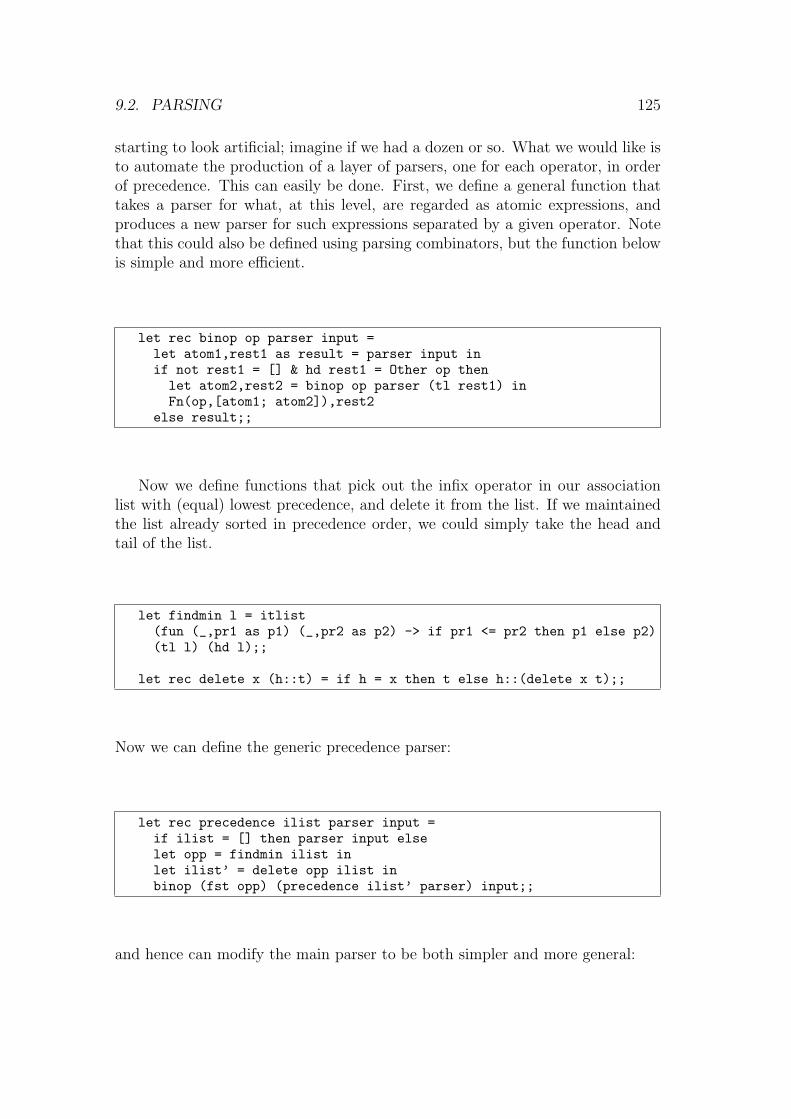
9.2. PARSING 125
starting to look artificial; imagine if we had a dozen or so. What we would like isto automate the production of a layer of parsers, one for each operator, in orderof precedence. This can easily be done. First, we define a general function thattakes a parser for what, at this level, are regarded as atomic expressions, andproduces a new parser for such expressions separated by a given operator. Notethat this could also be defined using parsing combinators, but the function belowis simple and more efficient.
let rec binop op parser input =let atom1,rest1 as result = parser input inif not rest1 = [] & hd rest1 = Other op thenlet atom2,rest2 = binop op parser (tl rest1) inFn(op,[atom1; atom2]),rest2
else result;;
Now we define functions that pick out the infix operator in our associationlist with (equal) lowest precedence, and delete it from the list. If we maintainedthe list already sorted in precedence order, we could simply take the head andtail of the list.
let findmin l = itlist(fun (_,pr1 as p1) (_,pr2 as p2) -> if pr1 <= pr2 then p1 else p2)(tl l) (hd l);;
let rec delete x (h::t) = if h = x then t else h::(delete x t);;
Now we can define the generic precedence parser:
let rec precedence ilist parser input =if ilist = [] then parser input elselet opp = findmin ilist inlet ilist’ = delete opp ilist inbinop (fst opp) (precedence ilist’ parser) input;;
and hence can modify the main parser to be both simpler and more general:

126 CHAPTER 9. EXAMPLES
let rec atom input= (name ++ a (Other "(") ++ termlist ++ a (Other ")")
>> (fun (((name,_),args),_) -> Fn(name,args))|| name
>> (fun s -> Var s)|| numeral
>> (fun s -> Const s)|| a (Other "(") ++ term ++ a (Other ")")
>> (snd o fst)|| a (Other "-") ++ atom
>> snd) inputand term input = precedence (!infixes) atom inputand termlist input
= (term ++ a (Other ",") ++ termlist>> (fun ((h,_),t) -> h::t)
|| term>> (fun h -> [h])) input;;
let parser = fst o (term ++ finished >> fst) o lex;;
for example:
#parser "2 * sin(x)^2 + 2 * sin(y)^2 - 2";;- : term =Fn("+",[Fn ("*", [Const "2"; Fn ("^", [Fn ("sin", [Var "x"]);
Const "2"])]);Fn("-",[Fn ("*", [Const "2"; Fn ("^", [Fn ("sin", [Var "y"]);
Const "2"])]);Const "2"])])
#install_printer "print_term";;- : unit = ()#parser "2 * sin(x)^2 + 2 * sin(y)^2 - 2";;- : term = ‘2 * sin(x) ^ 2 + (2 * sin(y) ^ 2 - 2)‘
9.2.6 Defects of our approach
Our approach to lexing and parsing is not particularly efficient. In fact, CAMLand some other ML implementations include a generator for LR parsers similar toYACC (Yet Another Compiler Compiler) which is often used to generate parsersin C under Unix. Not only are these more general in the grammars that theycan handle, but the resulting parsers are more efficient. However we believethe present approach is rather clear, adequate for most purposes, and a goodintroduction to programming with higher order functions.
The inefficiency of our approach can be reduced by avoiding a few particularlywasteful features. Note that if two different productions for the same syntactic
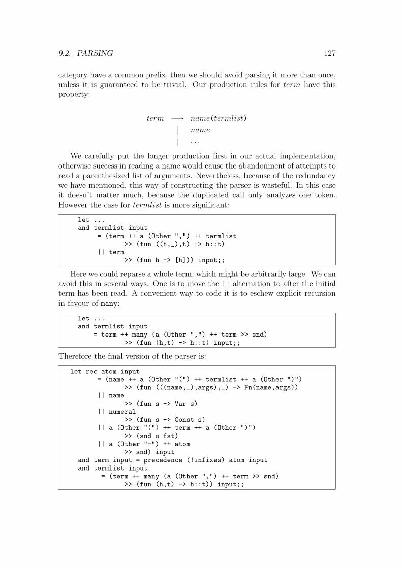
9.2. PARSING 127
category have a common prefix, then we should avoid parsing it more than once,unless it is guaranteed to be trivial. Our production rules for term have thisproperty:
term −→ name(termlist)
| name
| · · ·
We carefully put the longer production first in our actual implementation,otherwise success in reading a name would cause the abandonment of attempts toread a parenthesized list of arguments. Nevertheless, because of the redundancywe have mentioned, this way of constructing the parser is wasteful. In this caseit doesn’t matter much, because the duplicated call only analyzes one token.However the case for termlist is more significant:
let ...and termlist input
= (term ++ a (Other ",") ++ termlist>> (fun ((h,_),t) -> h::t)
|| term>> (fun h -> [h])) input;;
Here we could reparse a whole term, which might be arbitrarily large. We canavoid this in several ways. One is to move the || alternation to after the initialterm has been read. A convenient way to code it is to eschew explicit recursionin favour of many:
let ...and termlist input
= term ++ many (a (Other ",") ++ term >> snd)>> (fun (h,t) -> h::t) input;;
Therefore the final version of the parser is:
let rec atom input= (name ++ a (Other "(") ++ termlist ++ a (Other ")")
>> (fun (((name,_),args),_) -> Fn(name,args))|| name
>> (fun s -> Var s)|| numeral
>> (fun s -> Const s)|| a (Other "(") ++ term ++ a (Other ")")
>> (snd o fst)|| a (Other "-") ++ atom
>> snd) inputand term input = precedence (!infixes) atom inputand termlist input
= (term ++ many (a (Other ",") ++ term >> snd)>> (fun (h,t) -> h::t)) input;;

128 CHAPTER 9. EXAMPLES
A general defect of our approach, and recursive descent parsing generally, isthat so-called left recursion in productions causes problems. This is where a givencategory expands to a sequence including the category itself as the first item. Forexample, if we had wanted to make the addition operator left-associative in ourearlier grammar, we could have used:
term −→ term + mulexp
| mulexp
The naive transcription into ML would loop indefinitely, calling term on thesame subterm over and over. There are various slightly ad hoc ways of dealingwith this problem. For example, one can convert this use of recursion, which insome ways is rather gratuitous, into the explicit use of repetition. We can do thisusing standard combinators like many to return a list of ‘mulexp’s and then runover the list building the tree left-associated.
A final problem is that we do not handle errors very gracefully. We alwaysraise the exception Noparse, and this, when caught, initiates backtracking. How-ever this is not always appropriate for typical grammars. At best, it can causeexpensive reparsing, and can lead to baffling error indications at the top level.For example, on encountering 5 +, we expect a term following the +, and if wedon’t find one, we should generate a comprehensible exception for the user, ratherthan raise Noparse and perhaps initiate several other pointless attempts to parsethe expression in a different way.
9.3 Exact real arithmetic
Real arithmetic on computers is normally done via floating point approximations.In general, we can only manipulate a real number, either ourselves or inside acomputer, via some sort of finite representation. Some question how numbers canbe said to ‘exist’ if they have no finite representation. For example, Kroneckeraccepted integers and rationals because they can be written down explicitly, andeven algebraic numbers3 because they can be represented using the polynomialsof which they are solutions. However he rejected transcendental numbers becauseapparently they could not be represented finitely. Allegedly he he greeted thefamous proof by Lindemann (1882) that π is transcendental with the remark thatthis was ‘interesting, except that π does not exist’.
However, given our modern perspective, we can say that after all many morenumbers than Kronecker would have accepted do have a finite representation,namely the program, or in some more abstract sense the rule, used to calculate
3Algebraic numbers are those that are roots of polynomials with integer coefficients, e.g.√2, and transcendental numbers are ones that aren’t.

9.3. EXACT REAL ARITHMETIC 129
them to greater and greater precision. For example, we can write a programthat will produce for any argument n the first n digits of π. Alternatively it canproduce a rational number r such that |π − r| < 2−n. Whatever approach istaken to the successive approximation of a real number, the key point is that itsrepresentation, the program itself, is finite.
This works particularly nicely in a language like ML where higher order func-tions are available. What we have called a ‘program’ above will just be an MLfunction. We can actually represent the arithmetic operations on numbers ashigher order functions that, given functions for approximating x and y, will pro-duce new ones for approximating x + y, xy, sin(x) and so on, for a wide rangeof functions. In an ordinary programming language, we would need to definea concrete representation for programs, e.g. ‘Godel numbering’, and write aninterpreter for this representation.4
9.3.1 Representation of real numbers
Our approach is to represent a real x by a function fx : N → Z that for eachn ∈ N returns an approximation of x to within 2−n, appropriately scaled. In fact,we have:
|fx(n)− 2nx| < 1
This is of course equivalent to |fx(n)2n − x| < 1
2n . We could return a rationalapproximation directly, but it would still be convenient for the rationals to havedenominators that are all powers of some number, so that common denominatorsarising during addition don’t get too big. Performing the scaling directly seemssimpler, requiring only integer arithmetic. Our choice of the base 2 is largelyarbitrary. A lower base is normally advantageous because it minimizes the gran-ularity of the achievable accuracies. For example, if we used base 10, then evenif we only need to increase the accuracy of an approximation slightly, we have tostep up the requested accuracy by a factor of 10.
9.3.2 Arbitrary-precision integers
CAML’s standard integers (type int) have a severely limited range, so first of allwe need to set up a type of unlimited-precision integers. This is not so difficultto program, but is slightly tedious. Fortunately, the CAML release includes alibrary that gives a fast implementation of arbitrary precision integer (and in factrational) arithmetic. A version of CAML Light with this library pre-loaded isinstalled on Thor. Assuming you have used the following path setting:
4Effectively, we are manipulating functions ‘in extension’ rather than ‘in intension’, i.e. notconcerning ourselves with their representation.
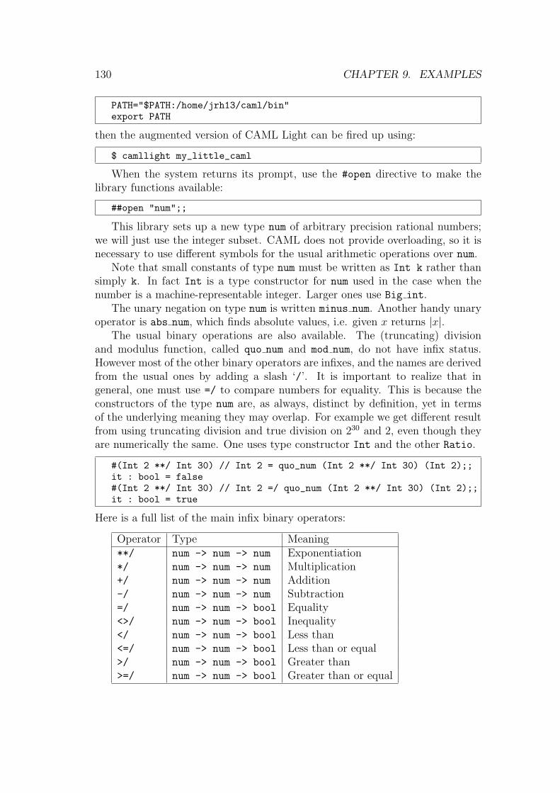
130 CHAPTER 9. EXAMPLES
PATH="$PATH:/home/jrh13/caml/bin"export PATH
then the augmented version of CAML Light can be fired up using:
$ camllight my_little_caml
When the system returns its prompt, use the #open directive to make thelibrary functions available:
##open "num";;
This library sets up a new type num of arbitrary precision rational numbers;we will just use the integer subset. CAML does not provide overloading, so it isnecessary to use different symbols for the usual arithmetic operations over num.
Note that small constants of type num must be written as Int k rather thansimply k. In fact Int is a type constructor for num used in the case when thenumber is a machine-representable integer. Larger ones use Big int.
The unary negation on type num is written minus num. Another handy unaryoperator is abs num, which finds absolute values, i.e. given x returns |x|.
The usual binary operations are also available. The (truncating) divisionand modulus function, called quo num and mod num, do not have infix status.However most of the other binary operators are infixes, and the names are derivedfrom the usual ones by adding a slash ‘/’. It is important to realize that ingeneral, one must use =/ to compare numbers for equality. This is because theconstructors of the type num are, as always, distinct by definition, yet in termsof the underlying meaning they may overlap. For example we get different resultfrom using truncating division and true division on 230 and 2, even though theyare numerically the same. One uses type constructor Int and the other Ratio.
#(Int 2 **/ Int 30) // Int 2 = quo_num (Int 2 **/ Int 30) (Int 2);;it : bool = false#(Int 2 **/ Int 30) // Int 2 =/ quo_num (Int 2 **/ Int 30) (Int 2);;it : bool = true
Here is a full list of the main infix binary operators:
Operator Type Meaning**/ num -> num -> num Exponentiation*/ num -> num -> num Multiplication+/ num -> num -> num Addition-/ num -> num -> num Subtraction=/ num -> num -> bool Equality<>/ num -> num -> bool Inequality</ num -> num -> bool Less than<=/ num -> num -> bool Less than or equal>/ num -> num -> bool Greater than>=/ num -> num -> bool Greater than or equal
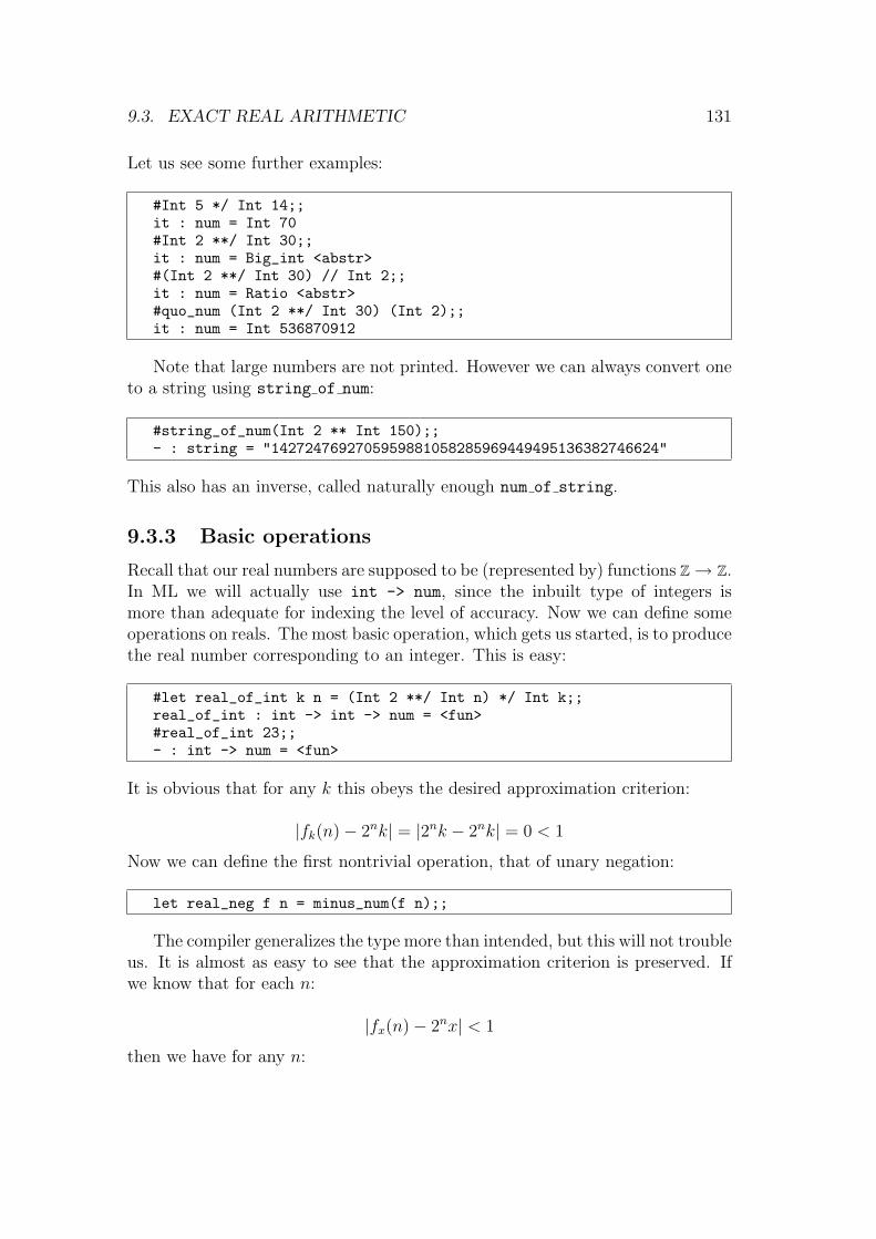
9.3. EXACT REAL ARITHMETIC 131
Let us see some further examples:
#Int 5 */ Int 14;;it : num = Int 70#Int 2 **/ Int 30;;it : num = Big_int <abstr>#(Int 2 **/ Int 30) // Int 2;;it : num = Ratio <abstr>#quo_num (Int 2 **/ Int 30) (Int 2);;it : num = Int 536870912
Note that large numbers are not printed. However we can always convert oneto a string using string of num:
#string_of_num(Int 2 ** Int 150);;- : string = "1427247692705959881058285969449495136382746624"
This also has an inverse, called naturally enough num of string.
9.3.3 Basic operations
Recall that our real numbers are supposed to be (represented by) functions Z → Z.In ML we will actually use int -> num, since the inbuilt type of integers ismore than adequate for indexing the level of accuracy. Now we can define someoperations on reals. The most basic operation, which gets us started, is to producethe real number corresponding to an integer. This is easy:
#let real_of_int k n = (Int 2 **/ Int n) */ Int k;;real_of_int : int -> int -> num = <fun>#real_of_int 23;;- : int -> num = <fun>
It is obvious that for any k this obeys the desired approximation criterion:
|fk(n)− 2nk| = |2nk − 2nk| = 0 < 1
Now we can define the first nontrivial operation, that of unary negation:
let real_neg f n = minus_num(f n);;
The compiler generalizes the type more than intended, but this will not troubleus. It is almost as easy to see that the approximation criterion is preserved. Ifwe know that for each n:
|fx(n)− 2nx| < 1
then we have for any n:

132 CHAPTER 9. EXAMPLES
|f−x(n)− 2n(−x)| = | − fx(n)− 2n(−x)|= | − (fx(n)− 2nx)|= |fx(n)− 2nx|< 1
Similarly, we can define an ‘absolute value’ function on real numbers, usingthe corresponding function abs num on numbers:
let real_abs f n = abs_num (f n);;
The correctness of this is again straightforward, using the fact that ||x|−|y|| ≤|x− y|. Now consider the problem of adding two real numbers. Suppose x and yare represented by fx and fy respectively. We could define:
fx+y(n) = fx(n) + fy(n)
However this gives no guarantee that the approximation criterion is main-tained; we would have:
|fx+y(n)− 2n(x + y)| = |fx(n) + fy(n)− 2n(x + y)|≤ |fx(n)− 2nx|+ |fy(n)− 2ny|
We can guarantee that the sum on the right is less than 2, but not that it isless than 1 as required. Therefore, we need in this case to evaluate x and y togreater accuracy than required in the answer. Suppose we define:
fx+y(n) = (fx(n + 1) + fy(n + 1))/2
Now we have:
|fx+y(n)− 2n(x + y)| = |(fx(n + 1) + fy(n + 1))/2− 2n(x + y)|≤ |fx(n + 1)/2− 2nx|+ |fy(n + 1)/2− 2ny|
=1
2|fx(n + 1)− 2n+1x|+ 1
2|fy(n + 1)− 2n+1y|
<1
21 +
1
21 = 1
Apparently this just gives the accuracy required. However we have implicitlyused real mathematical division above. Since the function is supposed to yield aninteger, we are obliged to round the quotient to an integer. If we just use quo num,the error from rounding this might be almost 1, after which we could never

9.3. EXACT REAL ARITHMETIC 133
guarantee the bound we want, however accurately we evaluate the arguments.However with a bit more care we can define a division function that alwaysreturns the integer closest to the true result (or one of them in the case of twoequally close ones), so that the rounding error never exceeds 1
2. This could be
done directly in integer arithmetic, but the most straightforward coding is to userational division followed by rounding to the nearest integer, as there are built-infunctions for both these operations:
#let ndiv x y = round_num(x // y);;ndiv : num -> num -> num = <fun>##infix "ndiv";;#(Int 23) ndiv (Int 5);;- : num = Int 5#(Int 22) ndiv (Int 5);;- : num = Int 4#(Int(-11)) ndiv (Int 4);;- : num = Int -3#(Int(-9)) ndiv (Int 4);;- : num = Int -2
Now if we define:
fx+y(n) = (fx(n + 2) + fy(n + 2)) ndiv 4
everything works:
|fx+y(n)− 2n(x + y)| = |((fx(n + 2) + fy(n + 2)) ndiv 4)− 2n(x + y)|
≤ 1
2+ |(fx(n + 2) + fy(n + 2))/4− 2n(x + y)|
=1
2+
1
4|(fx(n + 2) + fy(n + 2))− 2n+2(x + y)|
≤ 1
2+
1
4|fx(n + 2)− 2n+2x|+ 1
4|fy(n + 2)− 2n+2y|
<1
2+
1
41 +
1
41
= 1
Accordingly we make our definition:
let real_add f g n =(f(n + 2) +/ g(n + 2)) ndiv (Int 4);;
We can define subtraction similarly, but the simplest approach is to build itout of the functions that we already have:
#let real_sub f g = real_add f (real_neg g);;real_sub : (num -> num) -> (num -> num) -> num -> num = <fun>

134 CHAPTER 9. EXAMPLES
It is a bit trickier to define multiplication, inverses and division. Howeverthe cases where we multiply or divide by an integer are much easier and quitecommon. It is worthwhile implementing these separately as they can be mademore efficient. We define:
fmx(n) = (mfx(n + p + 1)) ndiv 2p+1
where p is chosen so that 2p ≥ |m|. For correctness, we have:
|fmx(n)− 2n(mx)| ≤ 1
2+ |mfx(n + p + 1)
2p+1− 2n(mx)|
=1
2+|m|2p+1
|fx(n + p + 1)− 2n+p+1x|
<1
2+|m|2p+1
≤ 1
2+
1
2
|m|2p
≤ 1
2+
1
2= 1
In order to implement this, we need a function to find the appropriate p. Thefollowing is crude but adequate:
let log2 =let rec log2 x y =if x </ Int 1 then yelse log2 (quo_num x (Int 2)) (y + 1) in
fun x -> log2 (x -/ Int 1) 0;;
The implementation is simply:
let real_intmul m x n =let p = log2 (abs_num m) inlet p1 = p + 1 in(m */ x(n + p1)) ndiv (Int 2 **/ Int p1);;
For division by an integer, we define:
fx/m(n) = fx(n) ndiv m
For correctness, we can ignore the trivial cases when m = 0, which shouldnever be used, and when m = ±1, since then the result is exact. Otherwise, weassume |fx(n)− 2nx| < 1, so |fx(n)/m− 2nx/m| < 1
|m| ≤12, which, together with
the fact that |fx(n) ndiv m− fx(n)/m| ≤ 12, yields the result. So we have:
let real_intdiv m x n =x(n) ndiv (Int m);;
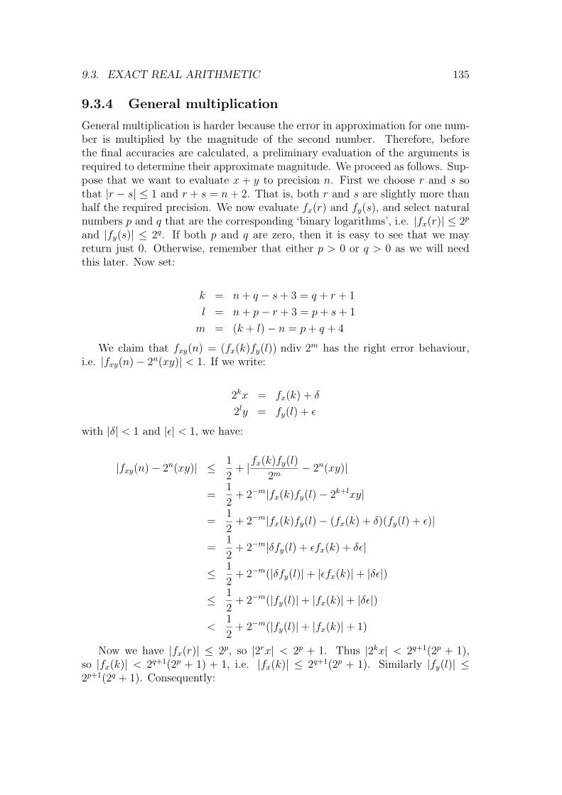
9.3. EXACT REAL ARITHMETIC 135
9.3.4 General multiplication
General multiplication is harder because the error in approximation for one num-ber is multiplied by the magnitude of the second number. Therefore, beforethe final accuracies are calculated, a preliminary evaluation of the arguments isrequired to determine their approximate magnitude. We proceed as follows. Sup-pose that we want to evaluate x + y to precision n. First we choose r and s sothat |r − s| ≤ 1 and r + s = n + 2. That is, both r and s are slightly more thanhalf the required precision. We now evaluate fx(r) and fy(s), and select naturalnumbers p and q that are the corresponding ‘binary logarithms’, i.e. |fx(r)| ≤ 2p
and |fy(s)| ≤ 2q. If both p and q are zero, then it is easy to see that we mayreturn just 0. Otherwise, remember that either p > 0 or q > 0 as we will needthis later. Now set:
k = n + q − s + 3 = q + r + 1
l = n + p− r + 3 = p + s + 1
m = (k + l)− n = p + q + 4
We claim that fxy(n) = (fx(k)fy(l)) ndiv 2m has the right error behaviour,i.e. |fxy(n)− 2n(xy)| < 1. If we write:
2kx = fx(k) + δ
2ly = fy(l) + ε
with |δ| < 1 and |ε| < 1, we have:
|fxy(n)− 2n(xy)| ≤ 1
2+ |fx(k)fy(l)
2m− 2n(xy)|
=1
2+ 2−m|fx(k)fy(l)− 2k+lxy|
=1
2+ 2−m|fx(k)fy(l)− (fx(k) + δ)(fy(l) + ε)|
=1
2+ 2−m|δfy(l) + εfx(k) + δε|
≤ 1
2+ 2−m(|δfy(l)|+ |εfx(k)|+ |δε|)
≤ 1
2+ 2−m(|fy(l)|+ |fx(k)|+ |δε|)
<1
2+ 2−m(|fy(l)|+ |fx(k)|+ 1)
Now we have |fx(r)| ≤ 2p, so |2rx| < 2p + 1. Thus |2kx| < 2q+1(2p + 1),so |fx(k)| < 2q+1(2p + 1) + 1, i.e. |fx(k)| ≤ 2q+1(2p + 1). Similarly |fy(l)| ≤2p+1(2q + 1). Consequently:

136 CHAPTER 9. EXAMPLES
|fy(l)|+ |fx(k)|+ 1 ≤ 2p+1(2q + 1) + 2q+1(2p + 1) + 1
= 2p+q+1 + 2p+1 + 2p+q+1 + 2q+1 + 1
= 2p+q+2 + 2p+1 + 2q+1 + 1
Now for our error bound we require |fy(l)| + |fx(k)| + 1 ≤ 2m−1, or dividingby 2 and using the discreteness of the integers:
2p+q+1 + 2p + 2q < 2p+q+2
We can write this as (2p+q +2p)+ (2p+q +2q) < 2p+q+1 +2p+q+1, which is truebecause we have either p > 0 or q > 0. So at last we are justified in defining:
let real_mul x y n =let n2 = n + 2 inlet r = n2 / 2 inlet s = n2 - r inlet xr = x(r)and ys = y(s) inlet p = log2 xrand q = log2 ys inif p = 0 & q = 0 then Int 0 elselet k = q + r + 1and l = p + s + 1and m = p + q + 4 in(x(k) */ y(l)) ndiv (Int 2 **/ Int m);;
9.3.5 Multiplicative inverse
Next we will define the multiplicative inverse function. In order to get any sortof upper bound on this, let alone a good approximation, we need to get a lowerbound for the argument. In general, there is no better way than to keep evaluatingthe argument with greater and greater accuracy until we can bound it away fromzero. We will use the following lemma to justify the correctness of our procedure:
Lemma 9.1 If 2e ≥ n + k + 1, |fx(k)| ≥ 2e and |fx(k)− 2kx| < 1, where fx(k)is an integer and e, n and k are natural numbers, then if we define
fy(n) = 2n+k ndiv fx(k)
we have |fy(n)− 2nx−1| < 1, i.e. the required bound.Proof: The proof is rather tedious and will not be given in full. We just sketchthe necessary case splits. If |fx(k)| > 2e then a straightforward analysis gives theresult; the rounding in ndiv gives an error of at most 1
2, and the remaining error
is < 12. If |fx(k)| = 2e but n + k ≥ e, then although the second component of the
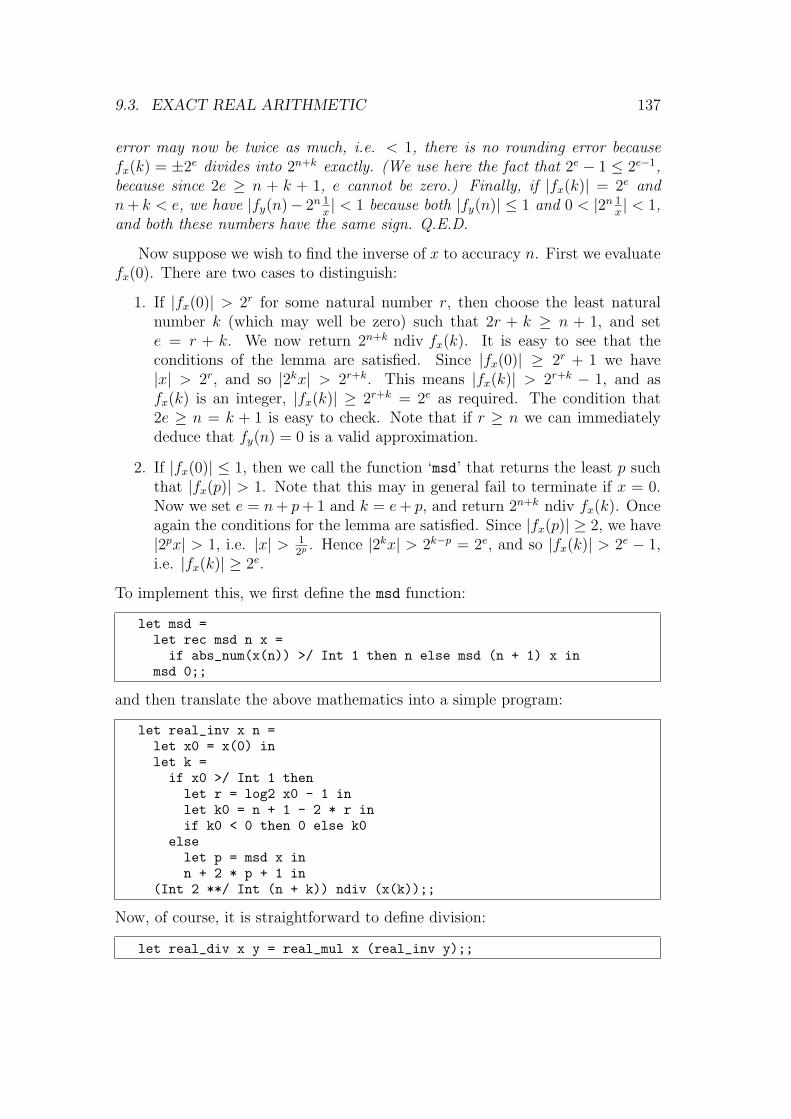
9.3. EXACT REAL ARITHMETIC 137
error may now be twice as much, i.e. < 1, there is no rounding error becausefx(k) = ±2e divides into 2n+k exactly. (We use here the fact that 2e − 1 ≤ 2e−1,because since 2e ≥ n + k + 1, e cannot be zero.) Finally, if |fx(k)| = 2e andn + k < e, we have |fy(n)− 2n 1
x| < 1 because both |fy(n)| ≤ 1 and 0 < |2n 1
x| < 1,
and both these numbers have the same sign. Q.E.D.
Now suppose we wish to find the inverse of x to accuracy n. First we evaluatefx(0). There are two cases to distinguish:
1. If |fx(0)| > 2r for some natural number r, then choose the least naturalnumber k (which may well be zero) such that 2r + k ≥ n + 1, and sete = r + k. We now return 2n+k ndiv fx(k). It is easy to see that theconditions of the lemma are satisfied. Since |fx(0)| ≥ 2r + 1 we have|x| > 2r, and so |2kx| > 2r+k. This means |fx(k)| > 2r+k − 1, and asfx(k) is an integer, |fx(k)| ≥ 2r+k = 2e as required. The condition that2e ≥ n = k + 1 is easy to check. Note that if r ≥ n we can immediatelydeduce that fy(n) = 0 is a valid approximation.
2. If |fx(0)| ≤ 1, then we call the function ‘msd’ that returns the least p suchthat |fx(p)| > 1. Note that this may in general fail to terminate if x = 0.Now we set e = n + p + 1 and k = e + p, and return 2n+k ndiv fx(k). Onceagain the conditions for the lemma are satisfied. Since |fx(p)| ≥ 2, we have|2px| > 1, i.e. |x| > 1
2p . Hence |2kx| > 2k−p = 2e, and so |fx(k)| > 2e − 1,i.e. |fx(k)| ≥ 2e.
To implement this, we first define the msd function:
let msd =let rec msd n x =if abs_num(x(n)) >/ Int 1 then n else msd (n + 1) x in
msd 0;;
and then translate the above mathematics into a simple program:
let real_inv x n =let x0 = x(0) inlet k =if x0 >/ Int 1 thenlet r = log2 x0 - 1 inlet k0 = n + 1 - 2 * r inif k0 < 0 then 0 else k0
elselet p = msd x inn + 2 * p + 1 in
(Int 2 **/ Int (n + k)) ndiv (x(k));;
Now, of course, it is straightforward to define division:
let real_div x y = real_mul x (real_inv y);;

138 CHAPTER 9. EXAMPLES
9.3.6 Ordering relations
The interesting things about all these functions is that they are in fact uncom-putable in general. The essential point is that it is impossible to decide whethera given number is zero. We can keep approximating it to greater and greateraccuracy, but if the approximations always return 0, we cannot tell whether it isgoing to do so indefinitely or whether the next step will give a nonzero answer.5
If x is not zero, then the search will eventually terminate, but if x is zero, it willrun forever.
Accepting this, it is not difficult to define the relational operators. To decidethe ordering relation of x and y it suffices to find an n such that |xn − yn| ≥ 2.For example, if xn ≥ yn + 2 we have
2nx > xn − 1 ≥ yn + 1 > 2ny
and so x > y. We first write a general procedure to perform this search, and thendefine all the orderings in terms of it. Note that the only way to arrive at thereflexive orderings is to justify the irreflexive version!
let separate =let rec separate n x y =let d = x(n) -/ y(n) inif abs_num(d) >/ Int 1 then delse separate (n + 1) x y in
separate 0;;
let real_gt x y = separate x y >/ Int 0;;let real_ge x y = real_gt x y;;let real_lt x y = separate x y </ Int 0;;let real_le x y = real_lt x y;;
9.3.7 Caching
In order to try out all the above functions, we would like to be able to printout a decimal representation of some approximation to a real. This is not hard,using some more standard facilities in the CAML library. If d decimal places aredesired, then we make n such that 2n > 10d and hence the accuracy correspondsat least to the number of digits printed.
let view x d =let n = 4 * d inlet out = x(n) // (Int 2 **/ Int n) inapprox_num_fix d out;;
5For a proof that it is uncomputable, simply wrap up the halting problem, by definingf(n) = 1 if a certain Turing machine has halted after no more than n iterations, and f(n) = 0otherwise.

9.3. EXACT REAL ARITHMETIC 139
Now we can test out some simple examples, which seem to work:
#let x = real_of_int 3;;x : int -> num = <fun>#let xi = real_inv x;;xi : int -> num = <fun>#let wun = real_mul x xi;;wun : int -> num = <fun>#view x 20;;it : string = "3.00000000000000000000"#view xi 20;;it : string = ".33333333333333333333"#view wun 20;;it : string = "1.00000000000000000000"
However there is a subtle and serious bug in our implementation, which showsitself if we try larger expressions. The problem is that subexpressions can beevaluated many times. Most obviously, this happens if they occur several timesin the input expression. But even if they don’t, the multiplication, and even moreso, the inverse, require trial evaluations at differing accuracies. As the evaluationpropagates down to the bottom level, there is often an exponential buildup ofreevaluations. For example, the following is slow — it takes several seconds.
#let x1 = real_of_int 1 inlet x2 = real_mul x1 x1 inlet x3 = real_mul x2 x2 inlet x4 = real_mul x3 x3 inlet x5 = real_mul x4 x4 inlet x6 = real_mul x5 x5 inlet x7 = real_mul x6 x6 inview x7 10;;- : string = "+1.0000000000"
We can fix this problem using the idea of caching or memo functions (Michie1968). We give each function a reference cell to remember the most accurateversion already calculated. If there is a second request for the same accuracy, itcan be returned immediately without further evaluation. What’s more, we canalways construct a lower-level approximation, say n, from a higher one, say n+kwith k ≥ 1. If we know that |fx(n + k)− 2n+kx| < 1 then we have:
|fx(n + k) ndiv 2k − 2nx| ≤ 1
2+ |fx(n + k)
2k− 2nx|
=1
2+
1
2k|fx(n + k)− 2n+kx|
<1
2+
1
2k
≤ 1

140 CHAPTER 9. EXAMPLES
Hence we are always safe in returning fx(n + k) ndiv 2k. We can implementthis memo technique via a generic function memo to be inserted in each of theprevious functions:
let real_of_int k = memo (fun n -> (Int 2 **/ Int n) */ Int k);;
let real_neg f = memo (fun n -> minus_num(f n));;
let real_abs f = memo (fun n -> abs_num (f n));;
let real_add f g = memo (fun n ->(f(n + 2) +/ g(n + 2)) ndiv (Int 4));;
let real_sub f g = real_add f (real_neg g);;
let real_intmul m x = memo (fun n ->let p = log2 (abs_num m) inlet p1 = p + 1 in(m */ x(n + p1)) ndiv (Int 2 **/ Int p1));;
let real_intdiv m x = memo (fun n ->x(n) ndiv (Int m));;
let real_mul x y = memo (fun n ->let n2 = n + 2 inlet r = n2 / 2 inlet s = n2 - r inlet xr = x(r)and ys = y(s) inlet p = log2 xrand q = log2 ys inif p = 0 & q = 0 then Int 0 elselet k = q + r + 1and l = p + s + 1and m = p + q + 4 in(x(k) */ y(l)) ndiv (Int 2 **/ Int m));;
let real_inv x = memo (fun n ->let x0 = x(0) inlet k =if x0 >/ Int 1 thenlet r = log2 x0 - 1 inlet k0 = n + 1 - 2 * r inif k0 < 0 then 0 else k0
elselet p = msd x inn + 2 * p + 1 in
(Int 2 **/ Int (n + k)) ndiv (x(k)));;
let real_div x y = real_mul x (real_inv y);;
where

9.4. PROLOG AND THEOREM PROVING 141
let memo f =let mem = ref (-1,Int 0) infun n -> let (m,res) = !mem in
if n <= m thenif m = n then reselse res ndiv (Int 2 **/ Int(m - n))
elselet res = f n inmem := (n,res); res;;
Now the above sequence of multiplications is instantaneous. Here are a fewmore examples:
#let pi1 = real_div (real_of_int 22) (real_of_int 7);;pi1 : int -> num = <fun>#view pi1 10;;it : string = "+3.1428571429"#let pi2 = real_div (real_of_int 355) (real_of_int 113);;pi2 : int -> num = <fun>#view pi2 10;;it : string = "+3.1415929204"#let pidiff = real_sub pi1 pi2;;pidiff : int -> num = <fun>#view pidiff 20;;it : string = "+0.00126422250316055626"#let ipidiff = real_inv pidiff;;ipidiff : int -> num = <fun>#view ipidiff 20;;it : string = "+791.00000000000000000000"
Of course, everything we have done to date could be done with rational arith-metic. Actually, it may happen that our approach is more efficient in certainsituations since we avoid calculating numbers that might have immense numer-ators and denominators when we just need an approximation. Nevertheless, thepresent approach really comes into its own when we want to define transcendentalfunctions like exp, sin etc. We will not cover this in detail for lack of space, butit makes an interesting exercise. One approach is to use truncated Taylor series.Note that finite summations can be evaluated directly rather than by iteratingthe addition function; this leads to much better error behaviour.
9.4 Prolog and theorem proving
The language Prolog is popular in Artificial Intelligence research, and is used invarious practical applications such as expert systems and intelligent databases.Here we will show how the main mechanism of Prolog, namely depth-first searchthrough a database of rules using unification and backtracking, can be imple-mented in ML. We do not pretend that this is a full-blown implementation of
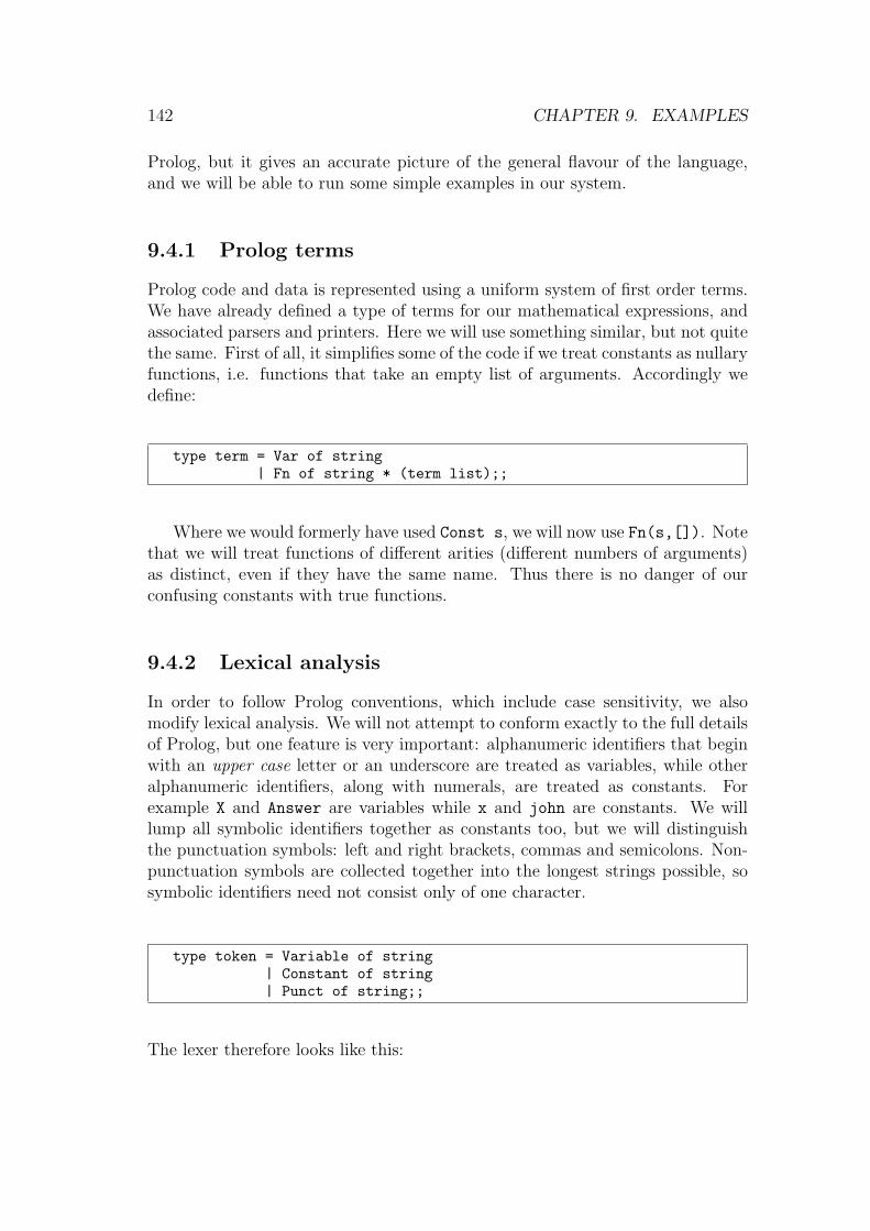
142 CHAPTER 9. EXAMPLES
Prolog, but it gives an accurate picture of the general flavour of the language,and we will be able to run some simple examples in our system.
9.4.1 Prolog terms
Prolog code and data is represented using a uniform system of first order terms.We have already defined a type of terms for our mathematical expressions, andassociated parsers and printers. Here we will use something similar, but not quitethe same. First of all, it simplifies some of the code if we treat constants as nullaryfunctions, i.e. functions that take an empty list of arguments. Accordingly wedefine:
type term = Var of string| Fn of string * (term list);;
Where we would formerly have used Const s, we will now use Fn(s,[]). Notethat we will treat functions of different arities (different numbers of arguments)as distinct, even if they have the same name. Thus there is no danger of ourconfusing constants with true functions.
9.4.2 Lexical analysis
In order to follow Prolog conventions, which include case sensitivity, we alsomodify lexical analysis. We will not attempt to conform exactly to the full detailsof Prolog, but one feature is very important: alphanumeric identifiers that beginwith an upper case letter or an underscore are treated as variables, while otheralphanumeric identifiers, along with numerals, are treated as constants. Forexample X and Answer are variables while x and john are constants. We willlump all symbolic identifiers together as constants too, but we will distinguishthe punctuation symbols: left and right brackets, commas and semicolons. Non-punctuation symbols are collected together into the longest strings possible, sosymbolic identifiers need not consist only of one character.
type token = Variable of string| Constant of string| Punct of string;;
The lexer therefore looks like this:

9.4. PROLOG AND THEOREM PROVING 143
let lex =let several p = many (some p) inlet collect(h,t) = h^(itlist (prefix ^) t "") inlet upper_alpha s = "A" <= s & s <= "Z" or s = "_"and lower_alpha s = "a" <= s & s <= "z" or "0" <= s & s <= "9"and punct s = s = "(" or s = ")" or s = "[" or s = "]"
or s = "," or s = "."and space s = s = " " or s = "\n" or s = "\t" inlet alphanumeric s = upper_alpha s or lower_alpha s inlet symbolic s = not space s & not alphanumeric s & not punct s inlet rawvariable =some upper_alpha ++ several alphanumeric >> (Variable o collect)
and rawconstant =(some lower_alpha ++ several alphanumeric ||some symbolic ++ several symbolic) >> (Constant o collect)
and rawpunct = some punct >> Punct inlet token =(rawvariable || rawconstant || rawpunct) ++several space >> fst in
let tokens = (several space ++ many token) >> snd inlet alltokens = (tokens ++ finished) >> fst infst o alltokens o explode;;
For example:
#lex "add(X,Y,Z) :- X is Y+Z.";;- : token list =[Constant "add"; Punct "("; Variable "X"; Punct ",";Variable "Y"; Punct ","; Variable "Z"; Punct ")";Constant ":-"; Variable "X"; Constant "is"; Variable "Y";Constant "+"; Variable "Z"; Punct "."]
9.4.3 Parsing
The basic parser is pretty much the same as before; the printer is exactly thesame. The main modification to the printer is that we allow Prolog lists to bewritten in a more convenient notation. Prolog has ‘.’ and ‘nil’ corresponding toML’s ‘::’ and ‘[]’, and we set up the parser so that lists can be written muchas in ML, e.g. ‘[1,2,3]’. We also allow the Prolog notation ‘[H|T]’ instead of‘cons(H,T)’, typically used for pattern-matching. After the basic functions:
let variable =fun (Variable s::rest) -> s,rest| _ -> raise Noparse;;
let constant =fun (Constant s::rest) -> s,rest| _ -> raise Noparse;;
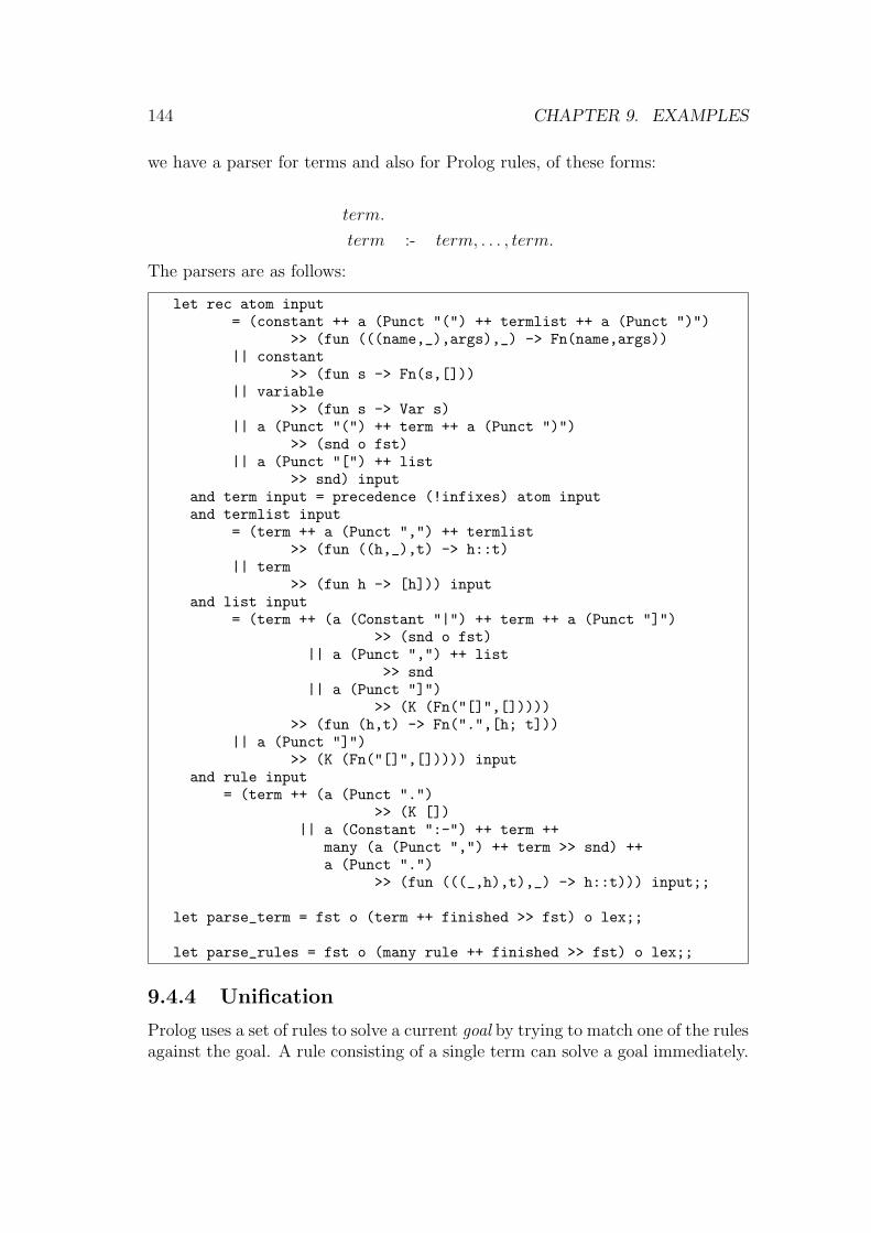
144 CHAPTER 9. EXAMPLES
we have a parser for terms and also for Prolog rules, of these forms:
term.
term :- term, . . . , term.
The parsers are as follows:
let rec atom input= (constant ++ a (Punct "(") ++ termlist ++ a (Punct ")")
>> (fun (((name,_),args),_) -> Fn(name,args))|| constant
>> (fun s -> Fn(s,[]))|| variable
>> (fun s -> Var s)|| a (Punct "(") ++ term ++ a (Punct ")")
>> (snd o fst)|| a (Punct "[") ++ list
>> snd) inputand term input = precedence (!infixes) atom inputand termlist input
= (term ++ a (Punct ",") ++ termlist>> (fun ((h,_),t) -> h::t)
|| term>> (fun h -> [h])) input
and list input= (term ++ (a (Constant "|") ++ term ++ a (Punct "]")
>> (snd o fst)|| a (Punct ",") ++ list
>> snd|| a (Punct "]")
>> (K (Fn("[]",[]))))>> (fun (h,t) -> Fn(".",[h; t]))
|| a (Punct "]")>> (K (Fn("[]",[])))) input
and rule input= (term ++ (a (Punct ".")
>> (K [])|| a (Constant ":-") ++ term ++
many (a (Punct ",") ++ term >> snd) ++a (Punct ".")
>> (fun (((_,h),t),_) -> h::t))) input;;
let parse_term = fst o (term ++ finished >> fst) o lex;;
let parse_rules = fst o (many rule ++ finished >> fst) o lex;;
9.4.4 Unification
Prolog uses a set of rules to solve a current goal by trying to match one of the rulesagainst the goal. A rule consisting of a single term can solve a goal immediately.

9.4. PROLOG AND THEOREM PROVING 145
In the case of a rule term :- term1, . . . , termn., if the goal matches term, thenProlog needs to solve each termi as a subgoal in order to finish the original goal.
However, goals and rules do not have to be exactly the same. Instead, Prologassigns variables in both the goal and the rule to make them match up, a processknown as unification. This means that we can end up proving a special case ofthe original goal, e.g. P (f(X)) instead of P (Y ). For example:
• To unify f(g(X), Y ) and f(g(a), X) we can set X = a and Y = a. Thenboth terms are f(g(a), a).
• To unify f(a, X, Y ) and f(X, a, Z) we can set X = a and Y = Z, and thenboth terms are f(a, a, Z).
• It is impossible to unify f(X) and X.
In general, unifiers are not unique. For example, in the second example wecould choose to set Y = f(b) and Z = f(b). However one can always choose onethat is most general, i.e. any other unification can be reached from it by furtherinstantiation (compare most general types in ML). In order to find it, roughlyspeaking, one need only descend the two terms recursively in parallel, and onfinding a variable on either side, assigns it to whatever the term on the otherside is. One also needs to check that the variable hasn’t already been assignedto something else, and that it doesn’t occur in the term being assigned to it (asin the last example above). A simple implementation of this idea follows. Wemaintain an association list giving instantiations already made, and we look eachvariable up to see if it is already assigned before proceeding. We use the existinginstantiations as an accumulator.
let rec unify tm1 tm2 insts =match tm1 withVar(x) ->(try let tm1’ = assoc x insts in
unify tm1’ tm2 instswith Not_found ->
augment (x,tm2) insts)| Fn(f1,args1) ->
match tm2 withVar(y) ->(try let tm2’ = assoc y insts in
unify tm1 tm2’ instswith Not_found ->
augment (y,tm1) insts)| Fn(f2,args2) ->
if f1 = f2then itlist2 unify args1 args2 instselse raise (error "functions do not match");;
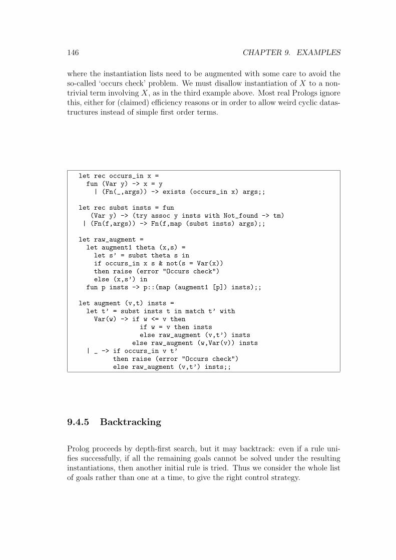
146 CHAPTER 9. EXAMPLES
where the instantiation lists need to be augmented with some care to avoid theso-called ‘occurs check’ problem. We must disallow instantiation of X to a non-trivial term involving X, as in the third example above. Most real Prologs ignorethis, either for (claimed) efficiency reasons or in order to allow weird cyclic datas-tructures instead of simple first order terms.
let rec occurs_in x =fun (Var y) -> x = y| (Fn(_,args)) -> exists (occurs_in x) args;;
let rec subst insts = fun(Var y) -> (try assoc y insts with Not_found -> tm)
| (Fn(f,args)) -> Fn(f,map (subst insts) args);;
let raw_augment =let augment1 theta (x,s) =let s’ = subst theta s inif occurs_in x s & not(s = Var(x))then raise (error "Occurs check")else (x,s’) in
fun p insts -> p::(map (augment1 [p]) insts);;
let augment (v,t) insts =let t’ = subst insts t in match t’ withVar(w) -> if w <= v then
if w = v then instselse raw_augment (v,t’) insts
else raw_augment (w,Var(v)) insts| _ -> if occurs_in v t’
then raise (error "Occurs check")else raw_augment (v,t’) insts;;
9.4.5 Backtracking
Prolog proceeds by depth-first search, but it may backtrack: even if a rule uni-fies successfully, if all the remaining goals cannot be solved under the resultinginstantiations, then another initial rule is tried. Thus we consider the whole listof goals rather than one at a time, to give the right control strategy.

9.4. PROLOG AND THEOREM PROVING 147
let rec first f =fun [] -> raise (error "No rules applicable")| (h::t) -> try f h with error _ -> first f t;;
let rec expand n rules insts goals =first (fun rule ->if goals = [] then insts elselet conc,asms =rename_rule (string_of_int n) rule in
let insts’ = unify conc (hd goals) insts inlet local,global = partition(fun (v,_) -> occurs_in v conc or
exists (occurs_in v) asms) insts’ inlet goals’ = (map (subst local) asms) @
(tl goals) inexpand (n + 1) rules global goals’) rules;;
Here we use a function ‘rename’ to generate fresh variables for the rules eachtime:
let rec rename s =fun (Var v) -> Var("~"^v^s)| (Fn(f,args)) -> Fn(f,map (rename s) args);;
let rename_rule s (conc,asms) =(rename s conc,map (rename s) asms);;
Finally, we can package everything together in a function prolog that triesto solve a given goal using the given rules:
type outcome = No | Yes of (string * term) list;;
let prolog rules goal =try let insts = expand 0 rules [] [goal] in
Yes(filter (fun (v,_) -> occurs_in v goal)insts)
with error _ -> No;;
This says either that the goal cannot be solved, or that it can be solved withthe given instantiations. Note that we only return one answer in this latter case,but this is easy to change if desired.
9.4.6 Examples
We can use the Prolog interpreter just written to try some simple examples fromProlog textbooks. For example:

148 CHAPTER 9. EXAMPLES
#let rules = parse_rules"male(albert).male(edward).female(alice).female(victoria).parents(edward,victoria,albert).parents(alice,victoria,albert).sister_of(X,Y) :-female(X),parents(X,M,F),parents(Y,M,F).";;
rules : (term * term list) list =[‘male(albert)‘, []; ‘male(edward)‘, [];‘female(alice)‘, []; ‘female(victoria)‘, [];‘parents(edward,victoria,albert)‘, [];‘parents(alice,victoria,albert)‘, [];‘sister_of(X,Y)‘,[‘female(X)‘; ‘parents(X,M,F)‘; ‘parents(Y,M,F)‘]]
#prolog rules ("sister_of(alice,edward)");;- : outcome = Yes []#prolog rules (parse_term "sister_of(alice,X)");;- : outcome = Yes ["X", ‘edward‘]#prolog rules (parse_term "sister_of(X,Y)");;- : outcome = Yes ["Y", ‘edward‘; "X", ‘alice‘]
The following are similar to some elementary ML list operations. Since Prologis relational rather than functional, it is possible to use Prolog queries in a moreflexible way, e.g. ask what arguments would give a certain result, rather thanvice versa:
#let r = parse_rules"append([],L,L).append([H|T],L,[H|A]) :- append(T,L,A).";;
r : (term * term list) list =[‘append([],L,L)‘, [];‘append(H . T,L,H . A)‘, [‘append(T,L,A)‘]]
#prolog r (parse_term "append([1,2],[3],[1,2,3])");;- : outcome = Yes []#prolog r (parse_term "append([1,2],[3,4],X)");;- : outcome = Yes ["X", ‘1 . (2 . (3 . (4 . [])))‘]#prolog r (parse_term "append([3,4],X,X)");;- : outcome = No#prolog r (parse_term "append([1,2],X,Y)");;- : outcome = Yes ["Y", ‘1 . (2 . X)‘]
In such cases, Prolog seems to be showing an impressive degree of intelligence.However under the surface it is just using a simple search strategy, and this caneasily be thwarted. For example, the following loops indefinitely:
#prolog r (parse_term "append(X,[3,4],X)");;
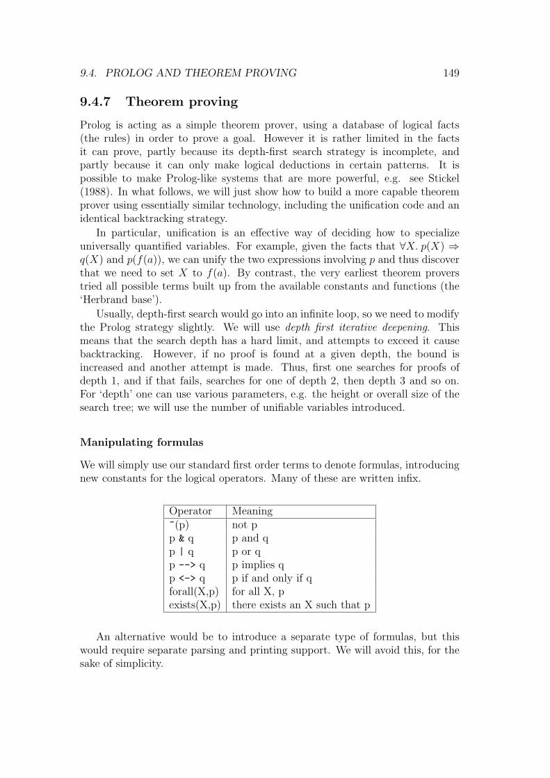
9.4. PROLOG AND THEOREM PROVING 149
9.4.7 Theorem proving
Prolog is acting as a simple theorem prover, using a database of logical facts(the rules) in order to prove a goal. However it is rather limited in the factsit can prove, partly because its depth-first search strategy is incomplete, andpartly because it can only make logical deductions in certain patterns. It ispossible to make Prolog-like systems that are more powerful, e.g. see Stickel(1988). In what follows, we will just show how to build a more capable theoremprover using essentially similar technology, including the unification code and anidentical backtracking strategy.
In particular, unification is an effective way of deciding how to specializeuniversally quantified variables. For example, given the facts that ∀X. p(X) ⇒q(X) and p(f(a)), we can unify the two expressions involving p and thus discoverthat we need to set X to f(a). By contrast, the very earliest theorem proverstried all possible terms built up from the available constants and functions (the‘Herbrand base’).
Usually, depth-first search would go into an infinite loop, so we need to modifythe Prolog strategy slightly. We will use depth first iterative deepening. Thismeans that the search depth has a hard limit, and attempts to exceed it causebacktracking. However, if no proof is found at a given depth, the bound isincreased and another attempt is made. Thus, first one searches for proofs ofdepth 1, and if that fails, searches for one of depth 2, then depth 3 and so on.For ‘depth’ one can use various parameters, e.g. the height or overall size of thesearch tree; we will use the number of unifiable variables introduced.
Manipulating formulas
We will simply use our standard first order terms to denote formulas, introducingnew constants for the logical operators. Many of these are written infix.
Operator Meaning~(p) not pp & q p and qp | q p or qp --> q p implies qp <-> q p if and only if qforall(X,p) for all X, pexists(X,p) there exists an X such that p
An alternative would be to introduce a separate type of formulas, but thiswould require separate parsing and printing support. We will avoid this, for thesake of simplicity.
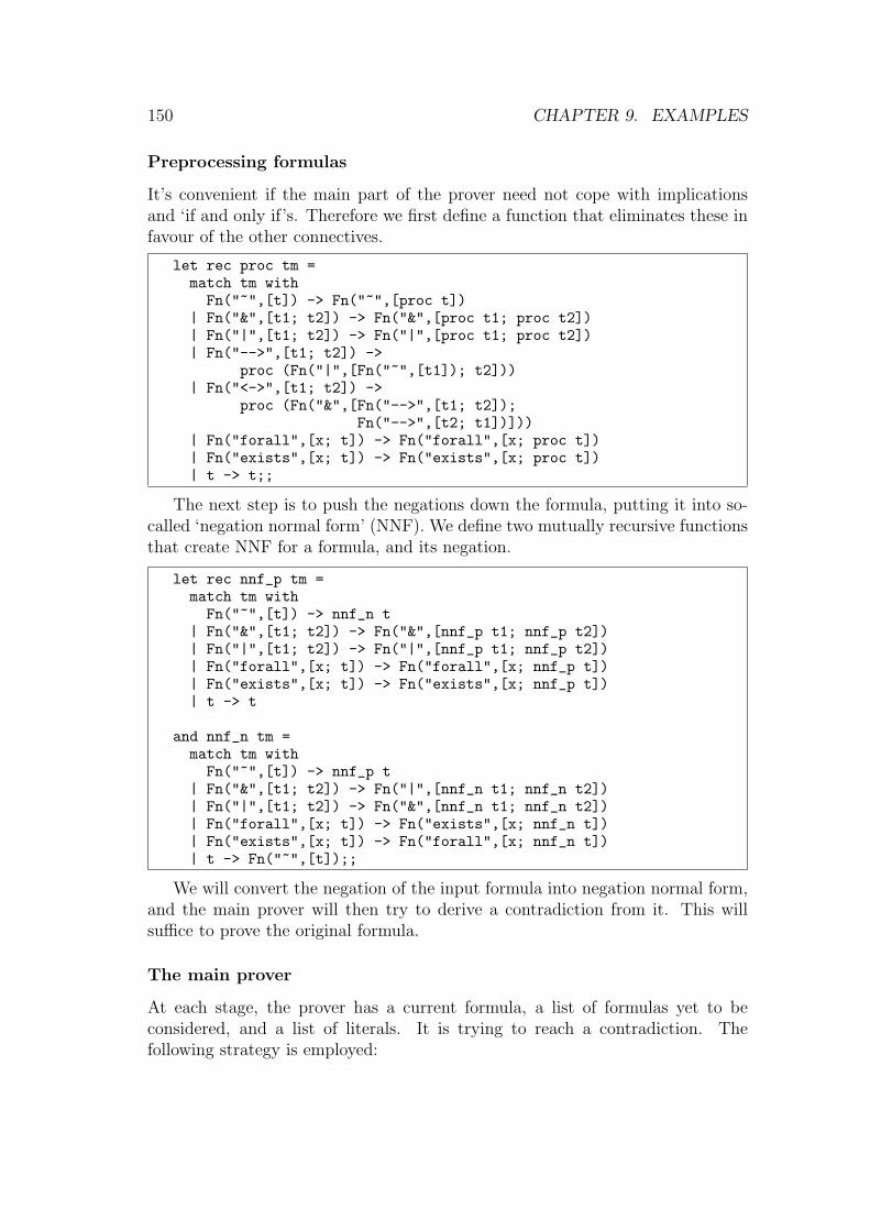
150 CHAPTER 9. EXAMPLES
Preprocessing formulas
It’s convenient if the main part of the prover need not cope with implicationsand ‘if and only if’s. Therefore we first define a function that eliminates these infavour of the other connectives.
let rec proc tm =match tm withFn("~",[t]) -> Fn("~",[proc t])
| Fn("&",[t1; t2]) -> Fn("&",[proc t1; proc t2])| Fn("|",[t1; t2]) -> Fn("|",[proc t1; proc t2])| Fn("-->",[t1; t2]) ->
proc (Fn("|",[Fn("~",[t1]); t2]))| Fn("<->",[t1; t2]) ->
proc (Fn("&",[Fn("-->",[t1; t2]);Fn("-->",[t2; t1])]))
| Fn("forall",[x; t]) -> Fn("forall",[x; proc t])| Fn("exists",[x; t]) -> Fn("exists",[x; proc t])| t -> t;;
The next step is to push the negations down the formula, putting it into so-called ‘negation normal form’ (NNF). We define two mutually recursive functionsthat create NNF for a formula, and its negation.
let rec nnf_p tm =match tm withFn("~",[t]) -> nnf_n t
| Fn("&",[t1; t2]) -> Fn("&",[nnf_p t1; nnf_p t2])| Fn("|",[t1; t2]) -> Fn("|",[nnf_p t1; nnf_p t2])| Fn("forall",[x; t]) -> Fn("forall",[x; nnf_p t])| Fn("exists",[x; t]) -> Fn("exists",[x; nnf_p t])| t -> t
and nnf_n tm =match tm withFn("~",[t]) -> nnf_p t
| Fn("&",[t1; t2]) -> Fn("|",[nnf_n t1; nnf_n t2])| Fn("|",[t1; t2]) -> Fn("&",[nnf_n t1; nnf_n t2])| Fn("forall",[x; t]) -> Fn("exists",[x; nnf_n t])| Fn("exists",[x; t]) -> Fn("forall",[x; nnf_n t])| t -> Fn("~",[t]);;
We will convert the negation of the input formula into negation normal form,and the main prover will then try to derive a contradiction from it. This willsuffice to prove the original formula.
The main prover
At each stage, the prover has a current formula, a list of formulas yet to beconsidered, and a list of literals. It is trying to reach a contradiction. Thefollowing strategy is employed:

9.4. PROLOG AND THEOREM PROVING 151
• If the current formula is ‘p & q’, then consider ‘p’ and ‘q’ separately, i.e.make ‘p’ the current formula and add ‘q’ to the formulas to be considered.
• If the current formula is ‘p | q’, then try to get a contradiction from ‘p’and then one from ‘q’.
• If the current formula is ‘forall(X,p)’, invent a new variable to replace ‘X’:the right value can be discovered later by unification.
• If the current formula is ‘exists(X,p)’, invent a new constant to replace ‘X’.
• Otherwise, the formula must be a literal, so try to unify it with a contra-dictory literal.
• If this fails, add it to the list of literals, and proceed with the next formula.
We desire a similar backtracking strategy to Prolog: only if the current in-stantiation allow all remaining goals to be solved do we accept it. We could uselists again, but instead we use continuations. A continuation is a function thatis passed to another function and can be called from within it to ‘perform therest of the computation’. In our case, it takes a list of instantiations and tries tosolve the remaining goals under these instantiations. Thus, rather than explicitlytrying to solve all remaining goals, we simply try calling the continuation.
let rec prove fm unexp pl nl n cont i =if n < 0 then raise (error "No proof") elsematch fm withFn("&",[p;q]) ->
prove p (q::unexp) pl nl n cont i| Fn("|",[p;q]) ->
prove p unexp pl nl n(prove q unexp pl nl n cont) i
| Fn("forall",[Var x; p]) ->let v = mkvar() inprove (subst [x,Var v] p) (unexp@[fm]) pl nl (n - 1) cont i
| Fn("exists",[Var x; p]) ->let v = mkvar() inprove (subst [x,Fn(v,[])] p) unexp pl nl (n - 1) cont i
| Fn("~",[t]) ->(try first (fun t’ -> let i’ = unify t t’ i in
cont i’) plwith error _ ->
prove (hd unexp) (tl unexp) pl (t::nl) n cont i)| t ->
(try first (fun t’ -> let i’ = unify t t’ i incont i’) nl
with error _ ->prove (hd unexp) (tl unexp) (t::pl) nl n cont i);;

152 CHAPTER 9. EXAMPLES
We set up the final prover as follows:
let prover =let rec prove_iter n t =try let insts = prove t [] [] [] n I [] in
let globinsts = filter(fun (v,_) -> occurs_in v t) insts in
n,globinstswith error _ -> prove_iter (n + 1) t in
fun t -> prove_iter 0 (nnf_n(proc(parse_term t)));;
This implements the iterative deepening strategy. It tries to find the proofwith the fewest universal instantiations; if it succeeds, it returns the number re-quired and any toplevel instantiations, throwing away instantiations for internallycreated variables.
Examples
Here are some simple examples from Pelletier (1986).
#let P1 = prover "p --> q <-> ~(q) --> ~(p)";;P1 : int * (string * term) list = 0, []#let P13 = prover "p | q & r <-> (p | q) & (p | r)";;P13 : int * (string * term) list = 0, []#let P16 = prover "(p --> q) | (q --> p)";;P16 : int * (string * term) list = 0, []#let P18 = prover "exists(Y,forall(X,p(Y)-->p(X)))";;P18 : int * (string * term) list = 2, []#let P19 = prover "exists(X,forall(Y,forall(Z,
(p(Y)-->q(Z))-->p(X)-->q(X))))";;P19 : int * (string * term) list = 6, []
A bigger example is the following:
#let P55 = prover"lives(agatha) & lives(butler) & lives(charles) &(killed(agatha,agatha) | killed(butler,agatha) |killed(charles,agatha)) &(forall(X,forall(Y,killed(X,Y) --> hates(X,Y) & ~(richer(X,Y))))) &
(forall(X,hates(agatha,X)--> ~(hates(charles,X)))) &
(hates(agatha,agatha) & hates(agatha,charles)) &(forall(X,lives(X) & ~(richer(X,agatha))
--> hates(butler,X))) &(forall(X,hates(agatha,X) --> hates(butler,X))) &(forall(X,~(hates(X,agatha)) | ~(hates(X,butler))
| ~(hates(X,charles))))--> killed(agatha,agatha)";;
P55 : int * (string * term) list = 6, []

9.4. PROLOG AND THEOREM PROVING 153
In fact, the prover can work out ‘whodunit’:
#let P55’ = prover"lives(agatha) & lives(butler) & lives(charles) &(killed(agatha,agatha) | killed(butler,agatha) |killed(charles,agatha)) &(forall(X,forall(Y,killed(X,Y) --> hates(X,Y) & ~(richer(X,Y))))) &
(forall(X,hates(agatha,X)--> ~(hates(charles,X)))) &
(hates(agatha,agatha) & hates(agatha,charles)) &(forall(X,lives(X) & ~(richer(X,agatha))
--> hates(butler,X))) &(forall(X,hates(agatha,X) --> hates(butler,X))) &(forall(X,~(hates(X,agatha)) | ~(hates(X,butler))
| ~(hates(X,charles))))--> killed(X,agatha)";;
P55’ : int * (string * term) list = 6, ["X", ‘agatha‘]
Further reading
Symbolic differentiation is a classic application of functional languages. Othersymbolic operations are major research issues in their own right — Davenport,Siret, and Tournier (1988) give a readable overview of what computer algebrasystems can do and how they work. Paulson (1983) discusses the kind of simpli-fication strategy we use here in a much more general setting.
Parsing with higher order functions is another popular example. It seems tohave existed in the functional programming folklore for a long time; an earlytreatment is given by Burge (1975). Our presentation has been influenced by thetreatments in Paulson (1991) and Reade (1989).
The first definition of ‘computable real number’ in our sense was in the orig-inal paper of Turing (1936). His approach was based on decimal expansions,but he needed to modify it (Turing 1937) for reasons explored in the exercisesbelow. The approach to real arithmetic given here follows the work of Boehm,Cartwright, O’Donnel, and Riggle (1986). More recently a high-performanceimplementation in CAML Light has been written by Menissier-Morain (1994),whose thesis (in French) contains detailed proofs of correctness for all the al-gorithms for elementary transcendental functions. For an alternative approachusing ‘linear fractional transformations’, see Potts (1996).
Our approach to Prolog search and backtracking, either using lists or contin-uations, is fairly standard. For more on implementing Prolog, see for exampleBoizumault (1993), while for more on the actual use of the language, the classictext by Clocksin and Mellish (1987) is recommended. A detailed discussion ofcontinuations in their many guises is given by Reynolds (1993). The unificationalgorithm given here is simple and purely functional, but rather inefficient. For

154 CHAPTER 9. EXAMPLES
faster imperative algorithms, see Martelli and Montanari (1982). Our theorem
prover is based on leanTAP (Beckert and Posegga 1995). For another importanttheorem proving method conveniently based on Prolog-style search, look at theProlog Technology Theorem Prover (Stickel 1988).
Exercises
1. Modify the printer so that each operator has an associativity, used whenprinting iterated cases of the operator to avoid excessive parentheses.
2. The differentiation rules for inverses 1/g(x) and quotients f(x)/g(x) arenot valid when g(x) = 0. Several others for functions like ln are also trueonly under certain conditions. Actually most commercial computer algebrasystems ignore this fact. However, try to do better, by writing a new versionof the differentiator that not only produces the derivative but also a list ofconditions that must be assumed for the derivative to be valid.
3. Try programming a simple procedure for indefinite integration. In general,it will not be able to do every integral, but try to make it understand a fewbasic principles.6
4. Read the documentation for the format library, and try to implement aprinter that behaves better when the output is longer than one line.
5. What happens if the parser functions like term, atom etc. are all eta-reducedby deleting the word input? What happens if precedence is consistentlyeta-reduced by deleting input?
6. How well do precedence parsers generated by precedence treat distinctoperators with the same precedence? How can the behaviour be improved?Can you extend it to allow a mix of left and right associative operators?For example, one really wants subtraction to associate to the left.
7. Rewrite the parser so that it gives helpful error messages when parsing fails.
8. Try representing a real number by the function that generates the first ndigits in a decimal expansion. Can you implement the addition function?
9. (*) How can you retain a positional representation while making the basicoperations computable?
6In fact there are algorithms that can integrate all algebraic expressions (not involving sin,ln etc.) — see Davenport (1981).
9.4. PROLOG AND THEOREM PROVING 155
10. Implement multiprecision integer arithmetic operations yourself. Make yourmultiplication algorithm O(nlog23) where n is the number of digits in thearguments.
11. Using memo as we have defined it, is it the case that whatever series ofarguments a function is applied to, it will always give the same answer forthe same argument? That is, are the functions true mathematical functionsdespite the internal use of references?
12. Write a parser-evaluator to read real-valued expressions and create the func-tional representation for the answer.
13. (*) Extend the real arithmetic routines to some functions like exp and sin.
14. Our preprocessing and negation normal form process can take exponentialtime in the length of the input in the case of many ‘if and only if’s. Modifyit so that it is linear in this number.
15. Extend the initial transformation into negation normal form so that it givesSkolem normal form.7
16. (*) Implement a more efficient unification algorithm, e.g. following Martelliand Montanari (1982).
17. (*) Implement a version of the Prolog Technology Theorem Prover (Stickel1988)
7Skolem normal form is covered in most elementary logic books, e.g. Enderton (1972).

Bibliography
Aagaard, M. and Leeser, M. (1994) Verifying a logic synthesis tool in Nuprl: Acase study in software verification. In v. Bochmann, G. and Probst, D. K.(eds.), Computer Aided Verification: Proceedings of the Fourth InternationalWorkshop, CAV’92, Volume 663 of Lecture Notes in Computer Science, Mon-treal, Canada, pp. 69–81. Springer Verlag.
Abramsky, S. (1990) The lazy lambda-calculus. In Turner, D. A. (ed.), ResearchTopics in Functional Programming, Year of Programming series, pp. 65–116.Addison-Wesley.
Adel’son-Vel’skii, G. M. and Landis, E. M. (1962) An algorithm for the organi-zation of information. Soviet Mathematics Doklady , 3, 1259–1262.
Backus, J. (1978) Can programming be liberated from the von Neumann style?A functional style and its algebra of programs. Communications of the ACM ,21, 613–641.
Barendregt, H. P. (1984) The Lambda Calculus: Its Syntax and Semantics, Vol-ume 103 of Studies in Logic and the Foundations of Mathematics. North-Holland.
Barwise, J. (1989) Mathematical proofs of computer correctness. Notices of theAmerican Mathematical Society , 7, 844–851.
Beckert, B. and Posegga, J. (1995) leanTAP : Lean, tableau-based deduction. Jour-nal of Automated Reasoning , 15, 339–358.
Boehm, H. J., Cartwright, R., O’Donnel, M. J., and Riggle, M. (1986) Exact realarithmetic: a case study in higher order programming. In Conference Record ofthe 1986 ACM Symposium on LISP and Functional Programming, pp. 162–173.Association for Computing Machinery.
Boizumault, P. (1993) The implementation of Prolog. Princeton series incomputer science. Princeton University Press. Translated from ‘Prolog:l’implantation’ by A. M. Djamboulian and J. Fattouh.
156

BIBLIOGRAPHY 157
Boyer, R. S. and Moore, J. S. (1979) A Computational Logic. ACM MonographSeries. Academic Press.
Burge, W. H. (1975) Recursive Programming Techniques. Addison-Wesley.
Church, A. (1936) An unsolvable problem of elementary number-theory. Ameri-can Journal of Mathematics , 58, 345–363.
Church, A. (1940) A formulation of the Simple Theory of Types. Journal ofSymbolic Logic, 5, 56–68.
Church, A. (1941) The calculi of lambda-conversion, Volume 6 of Annals of Math-ematics Studies. Princeton University Press.
Clocksin, W. F. and Mellish, C. S. (1987) Programming in Prolog (3rd ed.).Springer-Verlag.
Curry, H. B. (1930) Grundlagen der Kombinatorischen Logik. American Journalof Mathematics , 52, 509–536, 789–834.
Davenport, J. H. (1981) On the integration of algebraic functions, Volume 102 ofLecture Notes in Computer Science. Springer-Verlag.
Davenport, J. H., Siret, Y., and Tournier, E. (1988) Computer algebra: systemsand algorithms for algebraic computation. Academic Press.
Davis, M. D., Sigal, R., and Weyuker, E. J. (1994) Computability, complexity, andlanguages: fundamentals of theoretical computer science (2nd ed.). AcademicPress.
de Bruijn, N. G. (1972) Lambda calculus notation with nameless dummies, a toolfor automatic formula manipulation, with application to the Church-Rossertheorem. Indagationes Mathematicae, 34, 381–392.
DeMillo, R., Lipton, R., and Perlis, A. (1979) Social processes and proofs oftheorems and programs. Communications of the ACM , 22, 271–280.
Dijkstra, E. W. (1976) A Discipline of Programming. Prentice-Hall.
Enderton, H. B. (1972) A Mathematical Introduction to Logic. Academic Press.
Frege, G. (1893) Grundgesetze der Arithmetik begriffsschrift abgeleitet. Jena. Par-tial English translation by Montgomery Furth in ‘The basic laws of arithmetic.Exposition of the system’, University of California Press, 1964.
Girard, J.-Y., Lafont, Y., and Taylor, P. (1989) Proofs and Types, Volume 7of Cambridge Tracts in Theoretical Computer Science. Cambridge UniversityPress.

158 BIBLIOGRAPHY
Gordon, A. D. (1994) Functional Programming and Input/Output. DistinguishedDissertations in Computer Science. Cambridge University Press.
Gordon, M. J. C. (1988) Programming Language Theory and its Implementa-tion: applicative and imperative paradigms. Prentice-Hall International Seriesin Computer Science. Prentice-Hall.
Gordon, M. J. C., Milner, R., and Wadsworth, C. P. (1979) Edinburgh LCF: AMechanised Logic of Computation, Volume 78 of Lecture Notes in ComputerScience. Springer-Verlag.
Henson, M. C. (1987) Elements of functional languages. Blackwell Scientific.
Hindley, J. R. and Seldin, J. P. (1986) Introduction to Combinators and λ-Calculus, Volume 1 of London Mathematical Society Student Texts. CambridgeUniversity Press.
Hudak, P. (1989) Conception, evolution, and application of functional program-ming languages. ACM Computing Surveys , 21, 359–411.
Huet, G. (1980) Confluent reductions: abstract properties and applications toterm rewriting systems. Journal of the ACM , 27, 797–821.
Kleene, S. C. (1935) A theory of positive integers in formal logic. AmericanJournal of Mathematics , 57, 153–173, 219–244.
Lagarias, J. (1985) The 3x + 1 problem and its generalizations. The AmericanMathematical Monthly , 92, 3–23. Available on the Web as http://www.cecm.sfu.ca/organics/papers/lagarias/index.html.
Landin, P. J. (1966) The next 700 programming languages. Communications ofthe ACM , 9, 157–166.
Lindemann, F. (1882) Uber die Zahl π. Mathematische Annalen, 120, 213–225.
Mairson, H. G. (1990) Deciding ML typability is complete for deterministic expo-nential time. In Conference Record of the Seventeenth Annual ACM Symposiumon Principles of Programming Languages (POPL), San Francisco, pp. 382–401.Association for Computing Machinery.
Mairson, H. G. (1991) Outline of a proof theory of parametricity. In Hughes, J.(ed.), 1991 ACM Symposium on Functional Programming and Computer Archi-tecture, Volume 523 of Lecture Notes in Computer Science, Harvard University,pp. 313–327.
Martelli, A. and Montanari, U. (1982) An efficient unification algorithm. ACMTransactions on Programming Languages and Systems , 4, 258–282.

BIBLIOGRAPHY 159
Mauny, M. (1995) Functional programming using CAML Light. Available on theWeb from http://pauillac.inria.fr/caml/tutorial/index.html.
Menissier-Morain, V. (1994) Arithmetique exacte, conception, algorithmiqueet performances d’une implementation informatique en precision arbitraire.These, Universite Paris 7.
Michie, D. (1968) “Memo” functions and machine learning. Nature, 218, 19–22.
Milner, R. (1978) A theory of type polymorphism in programming. Journal ofComputer and Systems Sciences , 17, 348–375.
Mycroft, A. (1981) Abstract interpretation and optimising transformations ofapplicative programs. Technical report CST-15-81, Computer Science Depart-ment, Edinburgh University, King’s Buildings, Mayfield Road, Edinburgh EH93JZ, UK.
Neumann, P. G. (1995) Computer-related risks. Addison-Wesley.
Oppen, D. (1980) Prettyprinting. ACM Transactions on Programming Languagesand Systems , 2, 465–483.
Paulson, L. C. (1983) A higher-order implementation of rewriting. Science ofComputer Programming , 3, 119–149.
Paulson, L. C. (1991) ML for the Working Programmer. Cambridge UniversityPress.
Pelletier, F. J. (1986) Seventy-five problems for testing automatic theoremprovers. Journal of Automated Reasoning , 2, 191–216. Errata, JAR 4 (1988),235–236.
Peterson, I. (1996) Fatal Defect : Chasing Killer Computer Bugs. Arrow.
Potts, P. (1996) Computable real arithmetic using linear fractional trans-formations. Unpublished draft for PhD thesis, available on the Web ashttp://theory.doc.ic.ac.uk/~pjp/pub/phd/draft.ps.gz.
Raphael, B. (1966) The structure of programming languages. Communicationsof the ACM , 9, 155–156.
Reade, C. (1989) Elements of Functional Programming. Addison-Wesley.
Reynolds, J. C. (1993) The discoveries of continuations. Lisp and Symbolic Com-putation, 6, 233–247.
160 BIBLIOGRAPHY
Robinson, J. A. (1994) Logic, computers, Turing and von Neumann. In Furukawa,K., Michie, D., and Muggleton, S. (eds.), Machine Intelligence 13, pp. 1–35.Clarendon Press.
Schonfinkel, M. (1924) Uber die Bausteine der mathematischen Logik. Mathe-matische Annalen, 92, 305–316. English translation, ‘On the building blocksof mathematical logic’ in van Heijenoort (1967), pp. 357–366.
Schwichtenberg, H. (1976) Definierbare Funktionen im λ-Kalkul mit Typen.Arkhiv fur mathematische Logik und Grundlagenforschung , 17, 113–114.
Stickel, M. E. (1988) A Prolog Technology Theorem Prover: Implementation byan extended Prolog compiler. Journal of Automated Reasoning , 4, 353–380.
Turing, A. M. (1936) On computable numbers, with an application to theEntscheidungsproblem. Proceedings of the London Mathematical Society (2),42, 230–265.
Turing, A. M. (1937) Correction to Turing (1936). Proceedings of the LondonMathematical Society (2), 43, 544–546.
van Heijenoort, J. (ed.) (1967) From Frege to Godel: A Source Book in Mathe-matical Logic 1879–1931. Harvard University Press.
Whitehead, A. N. (1919) An Introduction to Mathematics. Williams and Norgate.
Whitehead, A. N. and Russell, B. (1910) Principia Mathematica (3 vols). Cam-bridge University Press.
Winskel, G. (1993) The formal semantics of programming languages: an intro-duction. Foundations of computing. MIT Press.
Wittgenstein, L. (1922) Tractatus Logico-Philosophicus. Routledge & KeganPaul.
Wright, A. (1996) Polymorphism for imperative languages without imperativetypes. Technical Report TR93-200, Rice University.