introduction to financial mathematicsfahim/intro_math_finance/textbook.pdf · introduction to...
TRANSCRIPT
Introduction to FinancialMathematics
Concepts and Computational Methods
Arash FahimFlorida State University
October 23, 2018

ii

Dedicated to Nasrin, Sevda and Idin.

iv

Notations
v
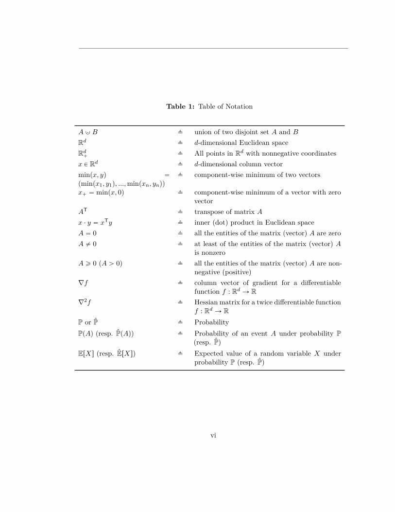
Table 1: Table of Notation
A Y B fi union of two disjoint set A and B
Rd fi d-dimensional Euclidean spaceRd
` fi All points in Rd with nonnegative coordinatesx P Rd fi d-dimensional column vectorminpx, yq “
pminpx1, y1q, ..., minpxn, ynqq
fi component-wise minimum of two vectors
x` “ minpx, 0q fi component-wise minimum of a vector with zerovector
AT fi transpose of matrix A
x ¨ y “ xTy fi inner (dot) product in Euclidean spaceA “ 0 fi all the entities of the matrix (vector) A are zeroA ‰ 0 fi at least of the entities of the matrix (vector) A
is nonzeroA ě 0 (A ą 0) fi all the entities of the matrix (vector) A are non-
negative (positive)∇f fi column vector of gradient for a differentiable
function f : Rd Ñ R∇2f fi Hessian matrix for a twice differentiable function
f : Rd Ñ RP or P fi ProbabilityPpAq (resp. PpAq) fi Probability of an event A under probability P
(resp. P)ErXs (resp. ErXs) fi Expected value of a random variable X under
probability P (resp. P)
vi

Preface
The story of this book started when I was assigned to teach an introductory financial math-ematics course at Florida State University. Originally, this course was all measure theory,integration and stochastic analysis. Then, it evolved to cover measure some probabilitytheory and option pricing in the binomial model. When I took over this course, I wasnot sure what I was going to do with it. However, I had a vision to educate studentsabout some new topics in financial mathematics. To start, I decided to take the advise ofa previous instructor to use a textbook by two authors, a quantitative financial analystsand a mathematician. The textbook was a little different and covered various models thatquants utilize in practice. The semester started, and as I was going through the first coupleof sections from the textbook, I realized that the book was unusable; many grave mistakesand wrong theorems, sloppy format, and coherency issues made it impossible for me toteach the course from this textbook. A few months later, I learned that another schoolhad had the same issue with the book as they invited one of the authors to teach a similarcourse. I now urgently needed a plan to save my course. So, I decided to write my ownlecture notes, and, over the past three years, these lecture notes grew and grew to includetopics that I consider useful for students to learn. In 2018, the Florida State Universitylibraries awarded me the “Alternative Textbook Grant” to help me make my lecture notesinto an open access free textbook. This current first edition is the result of many hours ofeffort by my library colleagues and myself.Many successful textbooks on financial mathematics have been developed in the recent
decades. My favorite ones are the two volumes by Steven Shreve, Stochastic Calculus forFinance I and II ; [31, 32]. They cover a large variety of topics in financial mathematicswith emphasis on the option pricing, the classical practice of quantitative financial analysts(quants). It also covers a great deal of stochastic calculus which is a basis for modelingalmost all financial assets. Option pricing remains a must-know for every quant and stochas-tic calculus is the language of the quantitative finance. However over time, a variety ofother subjects have been added to the list of what quants need to learn, including efficientcomputer programming, machine learning, data mining, big data, and so on. Many ofthese topics were irrelevant in 70s, when the quantitative finance was initially introduced.Since then, financial markets has changed in the tools that the traders use, and the speedof transactions. The amount of data that quants can use in their evaluation is too large to
vii
be handled by simple statistical techniques. Also, financial regulations has been adjustedto the new market environment. They now require financial institutions to measure somerisks that where not included in the classical risk management practice. For instance, af-ter the financial meltdown in 2007, systemic risk and central clearing became importantresearch areas for the regulator. In addition, a demand for more robust evaluation of risksled to researches in the robust risk management and model risk evaluations.As the financial mathematics career grows to cover the above-mentioned topics, the
prospect of the financial mathematics master’s programs must also become broader intopics. In the current book, I tried to include some new topics in an introductory level.One of the major challenges in teaching financial mathematics is the diverse background of
students, at least in some institutions such as Florida State University. For example, somestudents whom I observed during the last five years, have broad finance background but lackthe necessary mathematical background. They very much want to learn the mathematicalaspects, but with fewer details and stepping more quickly into the implementational aspects.Other students have majors in mathematics, engineering or computer science who needmore basic knowledge in finance. One thing that both groups need is to develop theirproblem-solving abilities. Current job market demand favors employees who can workindependently and solve hard problems, rather than those who simply take instructionsand implement them. Therefore, I designed this book to serve as an introductory course infinancial mathematics with focus on conceptual understanding of the models and problemsolving. It includes the mathematical background information needed for areas such asoption pricing as well as a basic financial knowledge of derivatives, bonds, and so on. Thegoal of the book is to expose the reader to a wide range of basic problems, some of whichemphasize analytic ability, some requiring programming techniques and others focusing onstatistical data analysis. In addition, it covers some areas which are outside the purview ofmainstream financial mathematics textbooks. For example, it presents marginal accountsetting by the CCP and systemic risk, and a brief overview of the model risk.One of the main drawbacks of commercial textbooks in financial mathematics is the lack
of flexibility to keep up with changes of the discipline. New editions often come far apartand with few changes. Also, it is not possible to modify them into the course needed fora specific program. The current book is a free, open textbook under a creative commonlicense with attribution. This allows instructors to use parts of this book to design theirown course in their own program, while adding new parts to keep up with the changes andthe institutional goals of their program.The first two chapters of this book only require calculus and introductory probability
and can be taught to senior undergraduate students. There is also a brief review of thesetopics in Sections A.1 and B of the appendix. I tried to be as brief as possible in theappendix; many books, including Stochastic Calculus for Finance I ([31, 32]) and ConvexOptimization ([9]), cover these topics extensively. My goal to include these topics is onlyto make the current book self-sufficient. The main goal of Chapter 1 is to familiarizethe reader with the basic concepts of risk management in financial mathematics. All
viii
these concepts are first introduced in a relatively nontechnical framework of one-periodsuch as Markowitz portfolio diversification or the Arrow-Debreu market model. Chapter2 generalizes the crucial results of the Arrow-Debreu market model to the multiperiodcase and introduces the multiperiod binomial model and the numerical methods based onit. Chapter 3 discusses more advanced subjects in probability, which are presented in theremainder of Section B and Section C of the appendix. This chapter is more appropriatefor graduate students. In Section 3.2, we first build important concepts and computationalmethods in continuous-time through the Bachelier model. Then, we provide the outline forthe more realistic Black-Scholes model in Section 3.3. Section 3.4 highlights the drawbacksof the Black-Scholes model with suggestions about how to remove them. Chapter 4 dealswith pricing a specific type of financial derivative: American options. Sections 4.0.1 and4.1 can be studied directly after finishing Chapter 2. The rest of this section requires anunderstanding of Section 3.3 as a prerequisite.
Acknowledgements•
ix

x
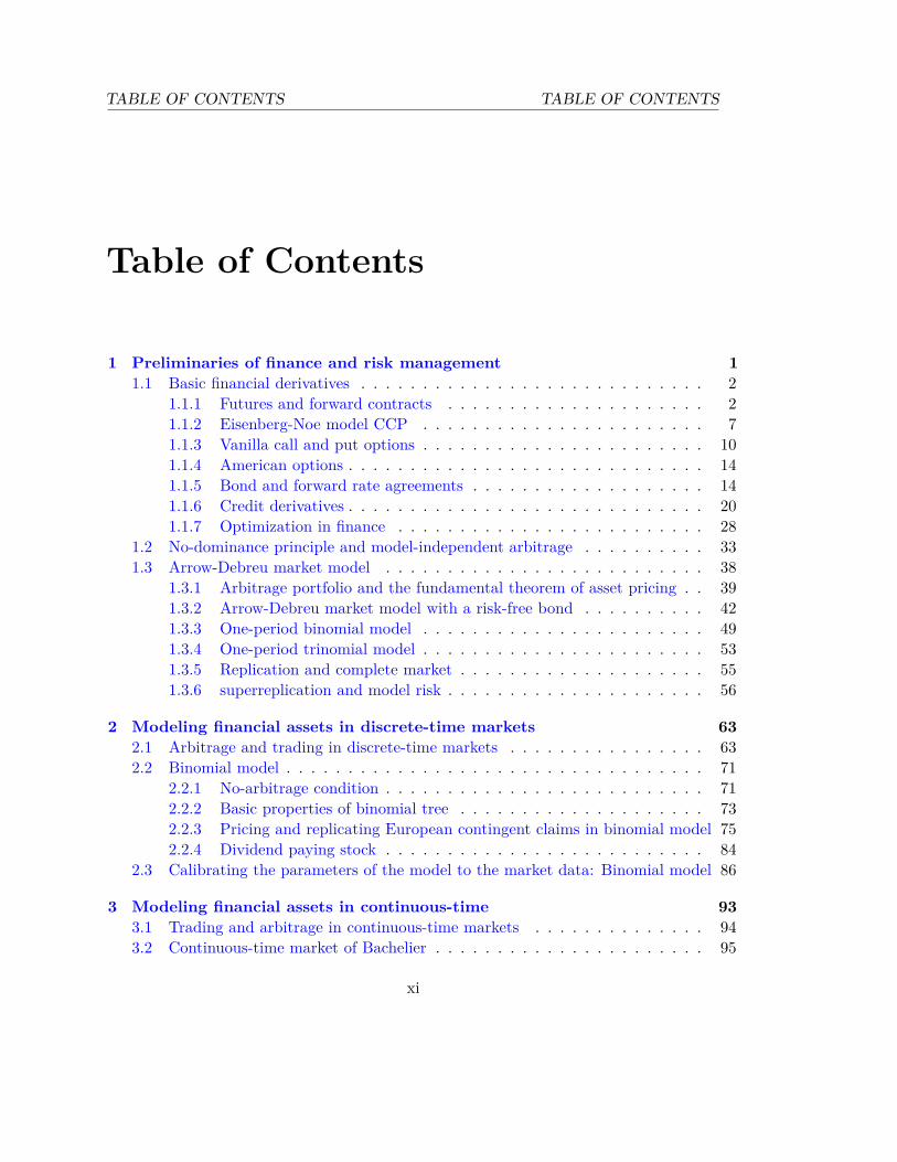
TABLE OF CONTENTS TABLE OF CONTENTS
Table of Contents
1 Preliminaries of finance and risk management 11.1 Basic financial derivatives . . . . . . . . . . . . . . . . . . . . . . . . . . . . 2
1.1.1 Futures and forward contracts . . . . . . . . . . . . . . . . . . . . . 21.1.2 Eisenberg-Noe model CCP . . . . . . . . . . . . . . . . . . . . . . . 71.1.3 Vanilla call and put options . . . . . . . . . . . . . . . . . . . . . . . 101.1.4 American options . . . . . . . . . . . . . . . . . . . . . . . . . . . . . 141.1.5 Bond and forward rate agreements . . . . . . . . . . . . . . . . . . . 141.1.6 Credit derivatives . . . . . . . . . . . . . . . . . . . . . . . . . . . . . 201.1.7 Optimization in finance . . . . . . . . . . . . . . . . . . . . . . . . . 28
1.2 No-dominance principle and model-independent arbitrage . . . . . . . . . . 331.3 Arrow-Debreu market model . . . . . . . . . . . . . . . . . . . . . . . . . . 38
1.3.1 Arbitrage portfolio and the fundamental theorem of asset pricing . . 391.3.2 Arrow-Debreu market model with a risk-free bond . . . . . . . . . . 421.3.3 One-period binomial model . . . . . . . . . . . . . . . . . . . . . . . 491.3.4 One-period trinomial model . . . . . . . . . . . . . . . . . . . . . . . 531.3.5 Replication and complete market . . . . . . . . . . . . . . . . . . . . 551.3.6 superreplication and model risk . . . . . . . . . . . . . . . . . . . . . 56
2 Modeling financial assets in discrete-time markets 632.1 Arbitrage and trading in discrete-time markets . . . . . . . . . . . . . . . . 632.2 Binomial model . . . . . . . . . . . . . . . . . . . . . . . . . . . . . . . . . . 71
2.2.1 No-arbitrage condition . . . . . . . . . . . . . . . . . . . . . . . . . . 712.2.2 Basic properties of binomial tree . . . . . . . . . . . . . . . . . . . . 732.2.3 Pricing and replicating European contingent claims in binomial model 752.2.4 Dividend paying stock . . . . . . . . . . . . . . . . . . . . . . . . . . 84
2.3 Calibrating the parameters of the model to the market data: Binomial model 86
3 Modeling financial assets in continuous-time 933.1 Trading and arbitrage in continuous-time markets . . . . . . . . . . . . . . 943.2 Continuous-time market of Bachelier . . . . . . . . . . . . . . . . . . . . . . 95
xi
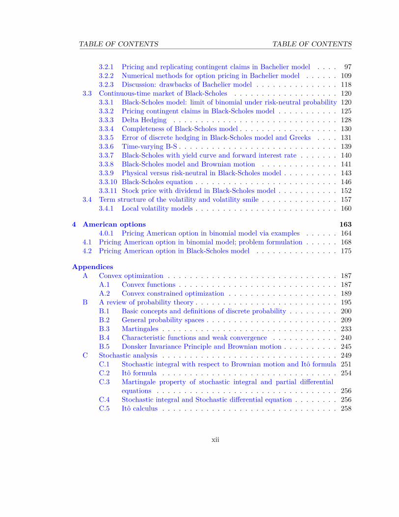
TABLE OF CONTENTS TABLE OF CONTENTS
3.2.1 Pricing and replicating contingent claims in Bachelier model . . . . 973.2.2 Numerical methods for option pricing in Bachelier model . . . . . . 1093.2.3 Discussion: drawbacks of Bachelier model . . . . . . . . . . . . . . . 118
3.3 Continuous-time market of Black-Scholes . . . . . . . . . . . . . . . . . . . 1203.3.1 Black-Scholes model: limit of binomial under risk-neutral probability 1203.3.2 Pricing contingent claims in Black-Scholes model . . . . . . . . . . . 1253.3.3 Delta Hedging . . . . . . . . . . . . . . . . . . . . . . . . . . . . . . 1283.3.4 Completeness of Black-Scholes model . . . . . . . . . . . . . . . . . . 1303.3.5 Error of discrete hedging in Black-Scholes model and Greeks . . . . 1313.3.6 Time-varying B-S . . . . . . . . . . . . . . . . . . . . . . . . . . . . . 1393.3.7 Black-Scholes with yield curve and forward interest rate . . . . . . . 1403.3.8 Black-Scholes model and Brownian motion . . . . . . . . . . . . . . 1413.3.9 Physical versus risk-neutral in Black-Scholes model . . . . . . . . . . 1433.3.10 Black-Scholes equation . . . . . . . . . . . . . . . . . . . . . . . . . . 1463.3.11 Stock price with dividend in Black-Scholes model . . . . . . . . . . . 152
3.4 Term structure of the volatility and volatility smile . . . . . . . . . . . . . . 1573.4.1 Local volatility models . . . . . . . . . . . . . . . . . . . . . . . . . . 160
4 American options 1634.0.1 Pricing American option in binomial model via examples . . . . . . 164
4.1 Pricing American option in binomial model; problem formulation . . . . . . 1684.2 Pricing American option in Black-Scholes model . . . . . . . . . . . . . . . 175
AppendicesA Convex optimization . . . . . . . . . . . . . . . . . . . . . . . . . . . . . . . 187
A.1 Convex functions . . . . . . . . . . . . . . . . . . . . . . . . . . . . . 187A.2 Convex constrained optimization . . . . . . . . . . . . . . . . . . . . 189
B A review of probability theory . . . . . . . . . . . . . . . . . . . . . . . . . . 195B.1 Basic concepts and definitions of discrete probability . . . . . . . . . 200B.2 General probability spaces . . . . . . . . . . . . . . . . . . . . . . . . 209B.3 Martingales . . . . . . . . . . . . . . . . . . . . . . . . . . . . . . . . 233B.4 Characteristic functions and weak convergence . . . . . . . . . . . . 240B.5 Donsker Invariance Principle and Brownian motion . . . . . . . . . . 245
C Stochastic analysis . . . . . . . . . . . . . . . . . . . . . . . . . . . . . . . . 249C.1 Stochastic integral with respect to Brownian motion and Itô formula 251C.2 Itô formula . . . . . . . . . . . . . . . . . . . . . . . . . . . . . . . . 254C.3 Martingale property of stochastic integral and partial differential
equations . . . . . . . . . . . . . . . . . . . . . . . . . . . . . . . . . 256C.4 Stochastic integral and Stochastic differential equation . . . . . . . . 256C.5 Itô calculus . . . . . . . . . . . . . . . . . . . . . . . . . . . . . . . . 258
xii

1. PRELIMINARIES
1
Preliminaries of finance and riskmanagement
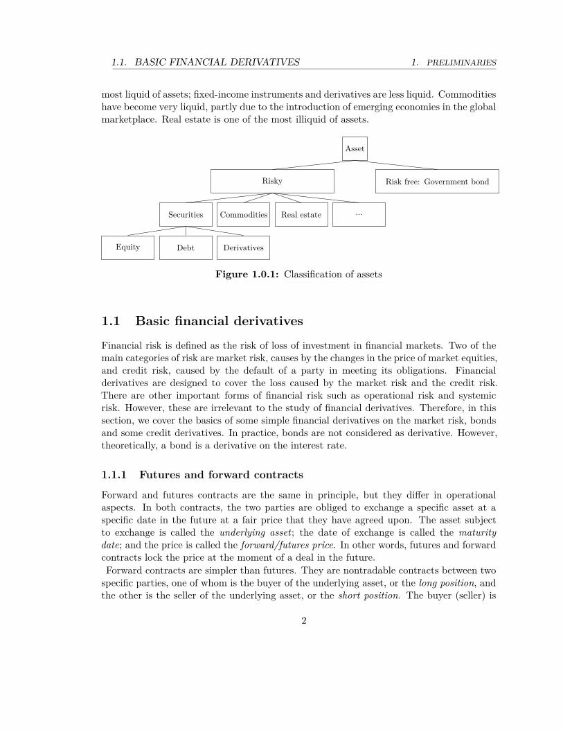
A risky asset is an asset with an uncertain future price, e.g. the stock of a company in anexchange market. Unlike a risky asset, a bank account with a fixed interest rate has an ab-solutely predictable value, and is called a risk-free asset. Risky assets are classified in manydifferent categories. Among them, financial securities, which constitute the largest body ofrisky assets, are traded in the exchange markets and are divided into three subcategories:equity, debt, and derivatives.An equity is a claim of ownership of a company. If it is issued by a corporation, it is called
common stock, stock, or share. Debt, sometimes referred to as a fixed-income instrument,promises a fixed cash flow until a time called maturity and is issued by an entity as a meansof borrowing through its sale. The cash flow from a fixed-income security is the return ofthe borrowed cash plus interest and is subject to default of the issuer, i.e., if the issuer isnot able to pay the cash flow at any of the promised dates. A derivatives is an asset whoseprice depends on a certain event. For example, a derivative can promise a payment (payoff)dependent on the price of a stock, the price of a fixed-income instrument, the default of acompany, or a climate event.An important class of assets that are not financial securities are described as commodities.
Broadly speaking, a commodity is an asset which is not a financial security but is stilltraded in a market, for example crops, energy, metals, and the like. Commodities are inparticular important because our daily life depends on them. Some of them are storablesuch as crops, which some others, such as electricity, are not. Some of them are subjectto seasonality, such as crops or oil. The other have a constant demand throughout theyear, for instance aluminum or copper. These various features of commodities introducechallenges in modeling commodity markets. There are other assets that are not usuallyincluded in any of the above classes, for instance real estate.If the asset is easily traded in an exchange market, it is called liquid. Equities are the
1
1.1. BASIC FINANCIAL DERIVATIVES 1. PRELIMINARIES
most liquid of assets; fixed-income instruments and derivatives are less liquid. Commoditieshave become very liquid, partly due to the introduction of emerging economies in the globalmarketplace. Real estate is one of the most illiquid of assets.
Asset
Risky
Securities
Equity Debt Derivatives
Commodities Real estate ...
Risk free: Government bond
Figure 1.0.1: Classification of assets
1.1 Basic financial derivatives
Financial risk is defined as the risk of loss of investment in financial markets. Two of themain categories of risk are market risk, causes by the changes in the price of market equities,and credit risk, caused by the default of a party in meeting its obligations. Financialderivatives are designed to cover the loss caused by the market risk and the credit risk.There are other important forms of financial risk such as operational risk and systemicrisk. However, these are irrelevant to the study of financial derivatives. Therefore, in thissection, we cover the basics of some simple financial derivatives on the market risk, bondsand some credit derivatives. In practice, bonds are not considered as derivative. However,theoretically, a bond is a derivative on the interest rate.
1.1.1 Futures and forward contracts
Forward and futures contracts are the same in principle, but they differ in operationalaspects. In both contracts, the two parties are obliged to exchange a specific asset at aspecific date in the future at a fair price that they have agreed upon. The asset subjectto exchange is called the underlying asset; the date of exchange is called the maturitydate; and the price is called the forward/futures price. In other words, futures and forwardcontracts lock the price at the moment of a deal in the future.Forward contracts are simpler than futures. They are nontradable contracts between two
specific parties, one of whom is the buyer of the underlying asset, or the long position, andthe other is the seller of the underlying asset, or the short position. The buyer (seller) is
2
1. PRELIMINARIES 1.1. FINANCIAL DERIVATIVES
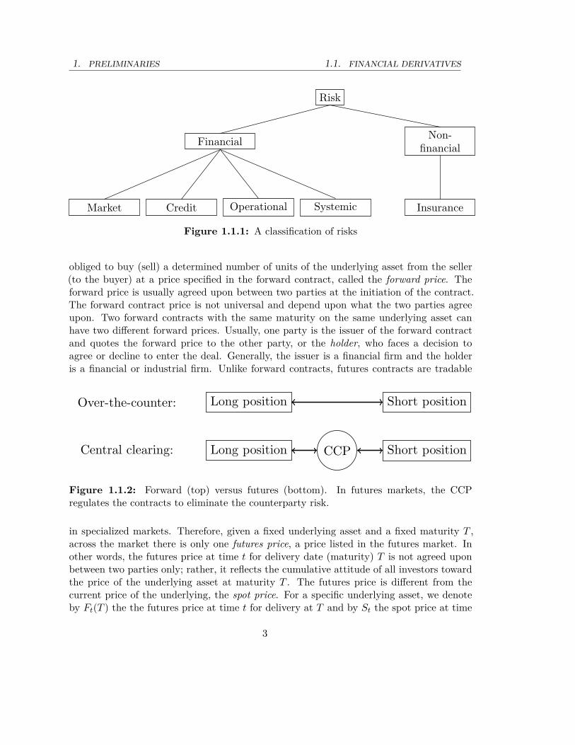
Risk
Financial
Market Credit Operational Systemic
Non-financial
Insurance
Figure 1.1.1: A classification of risks
obliged to buy (sell) a determined number of units of the underlying asset from the seller(to the buyer) at a price specified in the forward contract, called the forward price. Theforward price is usually agreed upon between two parties at the initiation of the contract.The forward contract price is not universal and depend upon what the two parties agreeupon. Two forward contracts with the same maturity on the same underlying asset canhave two different forward prices. Usually, one party is the issuer of the forward contractand quotes the forward price to the other party, or the holder, who faces a decision toagree or decline to enter the deal. Generally, the issuer is a financial firm and the holderis a financial or industrial firm. Unlike forward contracts, futures contracts are tradable
Over-the-counter: Long position Short position
Central clearing: Long position CCP Short position
Figure 1.1.2: Forward (top) versus futures (bottom). In futures markets, the CCPregulates the contracts to eliminate the counterparty risk.
in specialized markets. Therefore, given a fixed underlying asset and a fixed maturity T ,across the market there is only one futures price, a price listed in the futures market. Inother words, the futures price at time t for delivery date (maturity) T is not agreed uponbetween two parties only; rather, it reflects the cumulative attitude of all investors towardthe price of the underlying asset at maturity T . The futures price is different from thecurrent price of the underlying, the spot price. For a specific underlying asset, we denoteby FtpT q the the futures price at time t for delivery at T and by St the spot price at time
3
1.1. FINANCIAL DERIVATIVES 1. PRELIMINARIES
t . FtpT q and St are related through
limtÑT
FtpT q “ ST .
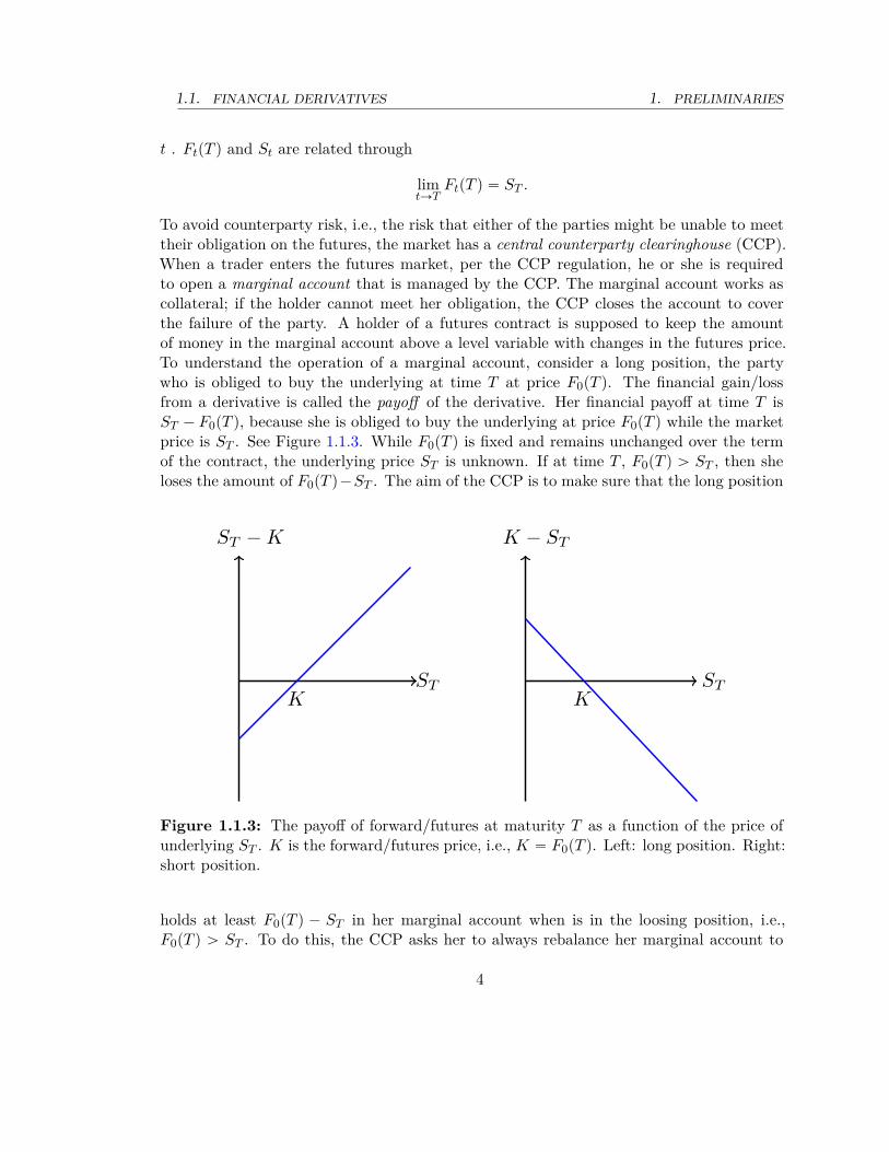
To avoid counterparty risk, i.e., the risk that either of the parties might be unable to meettheir obligation on the futures, the market has a central counterparty clearinghouse (CCP).When a trader enters the futures market, per the CCP regulation, he or she is requiredto open a marginal account that is managed by the CCP. The marginal account works ascollateral; if the holder cannot meet her obligation, the CCP closes the account to coverthe failure of the party. A holder of a futures contract is supposed to keep the amountof money in the marginal account above a level variable with changes in the futures price.To understand the operation of a marginal account, consider a long position, the partywho is obliged to buy the underlying at time T at price F0pT q. The financial gain/lossfrom a derivative is called the payoff of the derivative. Her financial payoff at time T isST ´ F0pT q, because she is obliged to buy the underlying at price F0pT q while the marketprice is ST . See Figure 1.1.3. While F0pT q is fixed and remains unchanged over the termof the contract, the underlying price ST is unknown. If at time T , F0pT q ą ST , then sheloses the amount of F0pT q´ST . The aim of the CCP is to make sure that the long position
K
ST −K
STK
K − ST
ST
Figure 1.1.3: The payoff of forward/futures at maturity T as a function of the price ofunderlying ST . K is the forward/futures price, i.e., K “ F0pT q. Left: long position. Right:short position.
holds at least F0pT q ´ ST in her marginal account when is in the loosing position, i.e.,F0pT q ą ST . To do this, the CCP asks her to always rebalance her marginal account to
4
1. PRELIMINARIES 1.1. FINANCIAL DERIVATIVES
keep it above pF0pT q ´ Stq`1 at any day t “ 0, ..., T to cover the possible future loss. An
example of marginal account rebalancing is shown in Table 1.1.
Time t 0 1 2 3 4Underlying asset price St 87.80 87.85 88.01 88.5 87.90Marginal account .20 .15 0 0 .10Changes to the marginal account – -.05 -.15 0 +.10
Table 1.1: Rebalancing the marginal account of a long position in futures with F0pT q=$88in four days.
The marginal account can be subject to several regulations, including minimum cashholdings. In this case, the marginal account holds the amount of pF0pT q ´ Stq` plus theminimum cash requirement. For more information of the mechanism of futures markets,see [19, Chapter 2].The existence of the marginal account creates an opportunity cost; the fund in the
marginal account can alternatively be invested somewhere else for profit, at least in arisk-free account with a fixed interest rate. The following example illustrates the opportu-nity cost.
Example 1.1.1 (Futures opportunity cost). Consider a futures contract with maturity Tof 2 days, a futures price equal to $99.95, and a forward contract with the same maturitybut a forward price of $100. Both contracts are written on the same risky asset with spotprice S0 “ $99.94. The marginal account for the futures contract has a $10 minimum cashrequirement and should by rebalanced daily thereafter according to the closing price. Wedenote the day-end price by S1 and S2 for day one and day two, respectively. Given thatthe risk-free daily compound interest rate is 0.2%, we want to find out for which valuesof the spot price of the underlying asset, pS1, S2q, the forward contract is more interestingthan the futures contract for long position.
Time t 0 1 2Underlying asset price St 99.94 S1 S2Marginal account 10.01 10+p99.95 ´ S1q` closed
The payoff of the forward contract for the long position is ST ´100, while the same quantityfor the futures is ST ´ 99.95. Therefore, the payoff of futures is worth .05 more than thepayoff of the forward on the maturity date T “ 2.However, there is an opportunity cost associated with futures contract. On day one, the
marginal account must have $10.01; the opportunity cost of holding $10.01 in the marginal
1pxq` :“ maxtx, 0u
5
1.1. FINANCIAL DERIVATIVES 1. PRELIMINARIES
account for day one is
p10.01qp1 ` .002q ´ 10.01 “ p10.01qp.002q “ .02002,
which is equivalent to p.02002qp1.002q “ .02006004 at the end of day two. On day two, wehave to keep $10 plus p99.95 ´ S1q` in the marginal account which creates an opportunitycost of p.002qp10 ` p99.95 ´ S1q`q. Therefore, the actual payoff of the futures contract iscalculated at maturity as
ST ´ 99.95 ´ p1.002q p.002qp10.01qloooooomoooooon
Opportunity cost of day 1
´p.002q p10 ` p99.95 ´ S1q`qloooooooooooomoooooooooooon
Opportunity cost of day 2
“ ST ´ 99.99006004 ´ p.002qp99.95 ´ S1q`.
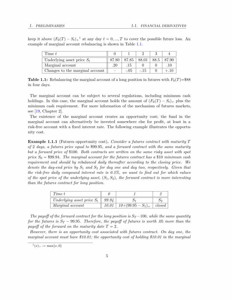
The total gain/loss of futures minus forward is
fpS1q :“ST ´ 99.99006004 ´ p.002qp99.95 ´ S1q` ´ ST ` 100“.00993996 ´ p.002qp99.95 ´ S1q`
shown in Figure 1.1.4,
99.9594.98002−.18996004
.00993996
f(S1)
S1
Figure 1.1.4: The difference between the gain of the futures and forward in Example1.1.1.
Exercise 1.1.1. Consider a futures contract with maturity T “ 2 days and futures priceequal to $100, and a forward contract with the same maturity and forward price of $99;both are written on a risky asset with price S0 “ $99. The marginal account for thefutures contract needs at least $20 upon entering the contract and should be rebalancedthereafter according to the spot price at the beginning of the day. Given that the risk-freedaily compound interest rate is 0.2%, for which values of the spot price of the underlyingasset, pS1, S2q, is the forward contract is more interesting than the futures contract for theshort position?A futures market provides easy access to futures contracts for a variety of products and
for different maturities. In addition, it makes termination of a contract possible. A longposition in a futures can even out his position by entering a short position of the samecontract.
6
1. PRELIMINARIES 1.1. FINANCIAL DERIVATIVES
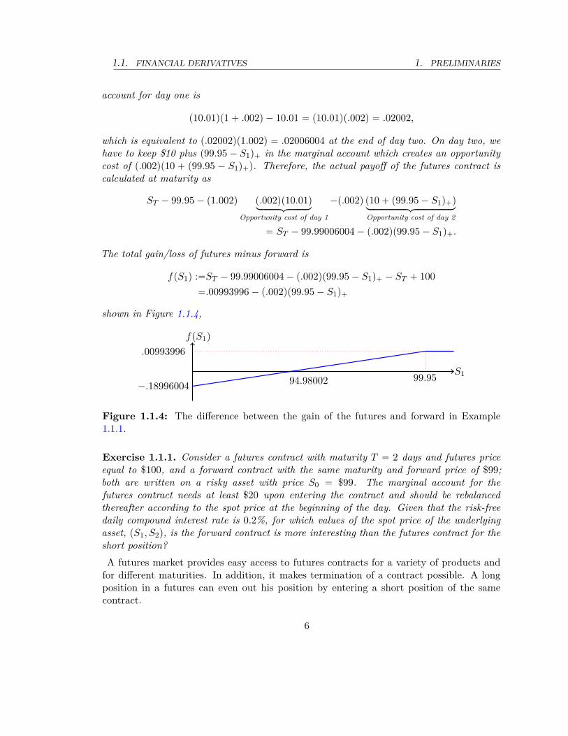
One of the practices in the futures market is rolling over. Imagine a trader who needsto have a contract on a product at a maturity T far in the future, such that there is nocontract in the futures market with such maturities. However, there is one with maturityT1 ă T . The trader can enter the futures with maturity T1 and later close it when amaturity T2 ą T1 become available. Then, he can continue thereafter until he reachescertain maturity T .It is well known that in an ideal situation, the spot price St of the underlying is less than or
equal to the forward/futures price FtpT q which is referred to as contango; see Proposition1.2.1 for a logical explanation of this phenomena. In reality, this result can no longer be true;especially for futures and forwards on commodities which typically incur storage cost ormay not even be storable. A situation in which the futures price of a commodity is less thanthe spot price is called normal backwardation or simply backwardation. Backwardation ismore common in commodities with relatively high storage cost; therefore, a low futuresprice provides an incentive to go into a futures contract. In contrast, when the storage costis negligible, then contango occurs. We close the discussion on futures and forward with
0 T
ST
Forward price (Contango)
Spot price
Forward price (Backwardation)
Figure 1.1.5: Contango vs backwardation. Recall that limtÑT FtpT q “ ST implies thatthe forward price and spot price must converge at maturity.
a model for CCP to determine the marginal account. Notice that the material in 1.1.2 isnot restricted to futures market CCP and can be generalized to any market monitored bythe CCP.
1.1.2 Eisenberg-Noe model CCP
The CCP can be a useful tool to control and manage systemic risk by setting capitalrequirements for the entities in a network of liabilities. Because if the marginal account
7

1.1. FINANCIAL DERIVATIVES 1. PRELIMINARIES
is not set properly, default of one entity can lead directly to a cascade of defaults. Legalaction against a defaulted entity is the last thing the CCP wants to do.Assume that there are N entities in a market and that Lij represents the amount that
entity i owes to entity j. Entity i has an equity (cash) balance of ci ě 0 in a marginalaccount with the CCP. The CCP wants to mediate by billing entity i amount pi as aclearing payment and use it to pay the debt of entity i to other entities. We introduce theliability matrix L consisting of all mutual liabilities Lij . It is obvious that Lii “ 0, sincethere is no self-liability.
L “
»
—
—
—
—
—
–
0 L1,2 ¨ ¨ ¨ L1,N´1 L1,N
L2,1 0 ¨ ¨ ¨ ¨ ¨ ¨ L2,N... . . . ...
LN´1,1 ¨ ¨ ¨ ¨ ¨ ¨ 0 LN´1,N
LN,1 LN,2 ¨ ¨ ¨ LN,N´1 0
fi
ffi
ffi
ffi
ffi
ffi
fl
We define Lj :“řN
i“1 Lji to be the total liability of entity j and define the weights πji :“ Lji
Lj
as the portion of total liability of entity j that is due to entity i. If a clearing payment pj
is made by entity j to the CCP, then entity i receives πjipj from the CCP. Therefore, afterall clearing payments p1, ..., pN are made, the entity i receives total of
řNj“1 πjipj . In [13],
the authors argue that a clearing payment pi must not exceed either the total liability Li
or the total amount of cash available by entity i.First, the Eisenberg-Noe model assume that the payment vector cannot increase the lia-
bility, i.e., pi ď Li for all i. Secondly, if the equity (cash) of entity i is given by ci, thenafter the clearing payment, the balance of the entity i, i.e., ci `
řNj“1 πjipj ´pi must remain
nonnegative. Therefore, the model suggests that the clearing payment p satisfies
pi “ min
#
Li , ci `
Nÿ
j“1πjipj
+
for all i.
In other word, the clearing payment vector p “ pp1, ..., pN q is therefore a fixed point ofthe map Φppq “ pΦ1ppq, ..., ΦN ppN qq, where the function Φ : r0, L1s ˆ ¨ ¨ ¨ ˆ r0, LN s Ñ
r0, L1s ˆ ¨ ¨ ¨ ˆ r0, LN s is given by
Φippq :“ min
#
Li , ci `
Nÿ
j“1πjipj
+
for i “ 1, .., N.
In general, the clearing payment vector p “ pp1, ..., pN q is not unique. The followingtheorem characterizes important properties of the clearing vector.
Theorem 1.1.1 ([13]). There are two clearing payment vectors pmax and pmin such thatfor any clearing payment p, we have pmin
i ď pi ď pmaxi for all i “ 1, ..., N .
8

1. PRELIMINARIES 1.1. FINANCIAL DERIVATIVES
In addition, the value of the equity of each entity remains unaffected by the choice of clearingvector payment; i.e., for all i “ 1, ..., N and for all clearing vector payments p,
ci `
Nÿ
j“1πjipj ´ pi “ ci `
Nÿ
j“1πjip
maxj ´ pmax
i “ ci `
Nÿ
j“1πjip
minj ´ pmin
i
Remark 1.1.1. The above theorem asserts that if by changing the clearing payment, entityi pays more to other entities, it is going to receive more so the total balance of the equityremains the same.
If an entity cannot clear all its liability with a payment vector, i.e., Li ą pi, then we saythat the entity has defaulted. Obviously, the equity of a defaulted entity vanishes. Thevanishing of an equity can also happen without default when ci `
řNj“1 πjipj “ pi “ Li.
A condition for the uniqueness of the clearing payment vector is provided in the originalwork of Eisenberg-Noe,[13]. However, the condition is restrictive and often hard to checkin a massive network of liabilities. On the other hand, the equity of each entity does notdepend on the choice of the payment vector. In a massive network, the problem of findingat least one payment vector can also be challenging. One of the ways to find a paymentvector is through solving a linear programming problem.
Theorem 1.1.2 ([13]). Let f : RN Ñ R be a strictly increasing function. Then, theminimizer of the following linear programming problem is a clearing payment vector.
max fppq subject to p ě 0, p ď L and p ď c ` pΠ, (1.1.1)
where c “ pc1, ..., cN q is the vector of the equities of the entities, L “ pL1, ..., LN q is thevector of the total liability of the entities, and Π is given by
Π “
»
—
—
—
—
—
–
0 π1,2 ¨ ¨ ¨ π1,N´1 π1,N
π2,1 0 ¨ ¨ ¨ ¨ ¨ ¨ π2,N... . . . ...
πN´1,1 ¨ ¨ ¨ ¨ ¨ ¨ 0 πN´1,N
πN,1 πN,2 ¨ ¨ ¨ πN,N´1 0
fi
ffi
ffi
ffi
ffi
ffi
fl
Exercise 1.1.2. Consider the liability matrix below by solving the linear programmingproblem (1.1.1) with fppq “
řNi“1 pi. Each row/column is an entity.
L “
»
—
—
–
0 1 0 10 0 2 02 0 0 10 5 0 0
fi
ffi
ffi
fl
The initial equities are given by c1 “ 1, c2 “ 2, c3 “ 0, and c4 “ 0.
9
1.1. FINANCIAL DERIVATIVES 1. PRELIMINARIES
a) By using a linear programming package such as linprog in MatLab, find a clearingpayment vector.
b) Mark the entities that default after applying the the clearing payment vector found inpart (a).
c) Increase the value of the equity of the defaulted entities just as much as they do notdefault anymore.
1.1.3 Vanilla call and put options
A call option gives the holder the right but not the obligation to buy a certain asset ata specified time in the future at a predetermined price. The specified time is called thematurity and often is denoted by T , and the predetermined price is called the strike priceand is denoted by K. Therefore, a call option protects its owner against any increasein the price of the underlying asset above the strike price at maturity. The asset priceat time t is denoted by St and at the maturity by ST . Call options are available in thespecialized options markets at a price that depends, among other factors, on time t, T , K,and spot price at current time St “ S. To simplify, we denote the price of a call option byCpT, K, S, tq2 to emphasize the main factors, i.e., t, T , K, and spot price at current timeS. Another type of vanilla option, the put option, protects its owner against any increasein the price of the underlying asset above the strike price at the maturity; i.e., it promisesthe seller of the underlying asset at least the strike price at maturity. The price of putoption is denoted by P pT, K, S, tq, or simply P when appropriate.The payoff of an option is the owner’s gain in a dollar amount. For instance, the payoff
of a call option is pST ´ Kq`. This is because, when the market price at maturity is ST
and the strike price is K, the holder of the option is buying the underlying asset at lowerprice K and gains ST ´ K, provided ST ą K. Otherwise, when ST ď K, the holder doesnot exercise the option and buys the asset from the market directly. Similarly, the payoffof a put option is pK ´ ST q`.Similar to futures, options are also traded in specialized markets. You can see option
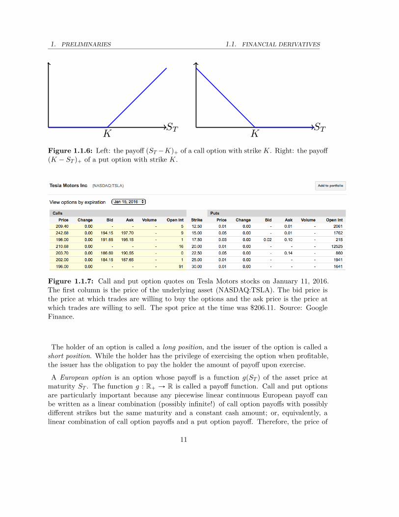
chain for Tesla Motors in Figure 1.1.7. The columns“bid” and “ask” indicate the best buyand sell prices in the outstanding orders, and column“Open Int” (open interest) shows thetotal volume of outstanding orders.When the spot price St of the underlying asset is greater than K, we say that the call
options are in-the-money and the puts options are out-of-the-money. Otherwise, whenSt ă K, the put options are in-the-money and the call options are out-of-the-money. If thestrike price K is (approximately) the same as spot price St, we call the option at-the-money(or ATM).
Far in-the-money call or put options are behave like forward contracts but with a wrongforward price! Similarly, far out-of-the-money call or put options have negligible worth.
2We will see later that C only depends on T ´ t in many models.
10
1. PRELIMINARIES 1.1. FINANCIAL DERIVATIVES
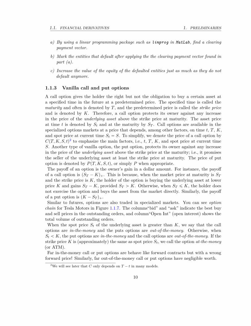
K KST ST
Figure 1.1.6: Left: the payoff pST ´Kq` of a call option with strike K. Right: the payoffpK ´ ST q` of a put option with strike K.
Figure 1.1.7: Call and put option quotes on Tesla Motors stocks on January 11, 2016.The first column is the price of the underlying asset (NASDAQ:TSLA). The bid price isthe price at which trades are willing to buy the options and the ask price is the price atwhich trades are willing to sell. The spot price at the time was $206.11. Source: GoogleFinance.
The holder of an option is called a long position, and the issuer of the option is called ashort position. While the holder has the privilege of exercising the option when profitable,the issuer has the obligation to pay the holder the amount of payoff upon exercise.
A European option is an option whose payoff is a function gpST q of the asset price atmaturity ST . The function g : R` Ñ R is called a payoff function. Call and put optionsare particularly important because any piecewise linear continuous European payoff canbe written as a linear combination (possibly infinite!) of call option payoffs with possiblydifferent strikes but the same maturity and a constant cash amount; or, equivalently, alinear combination of call option payoffs and a put option payoff. Therefore, the price of
11
1.1. FINANCIAL DERIVATIVES 1. PRELIMINARIES
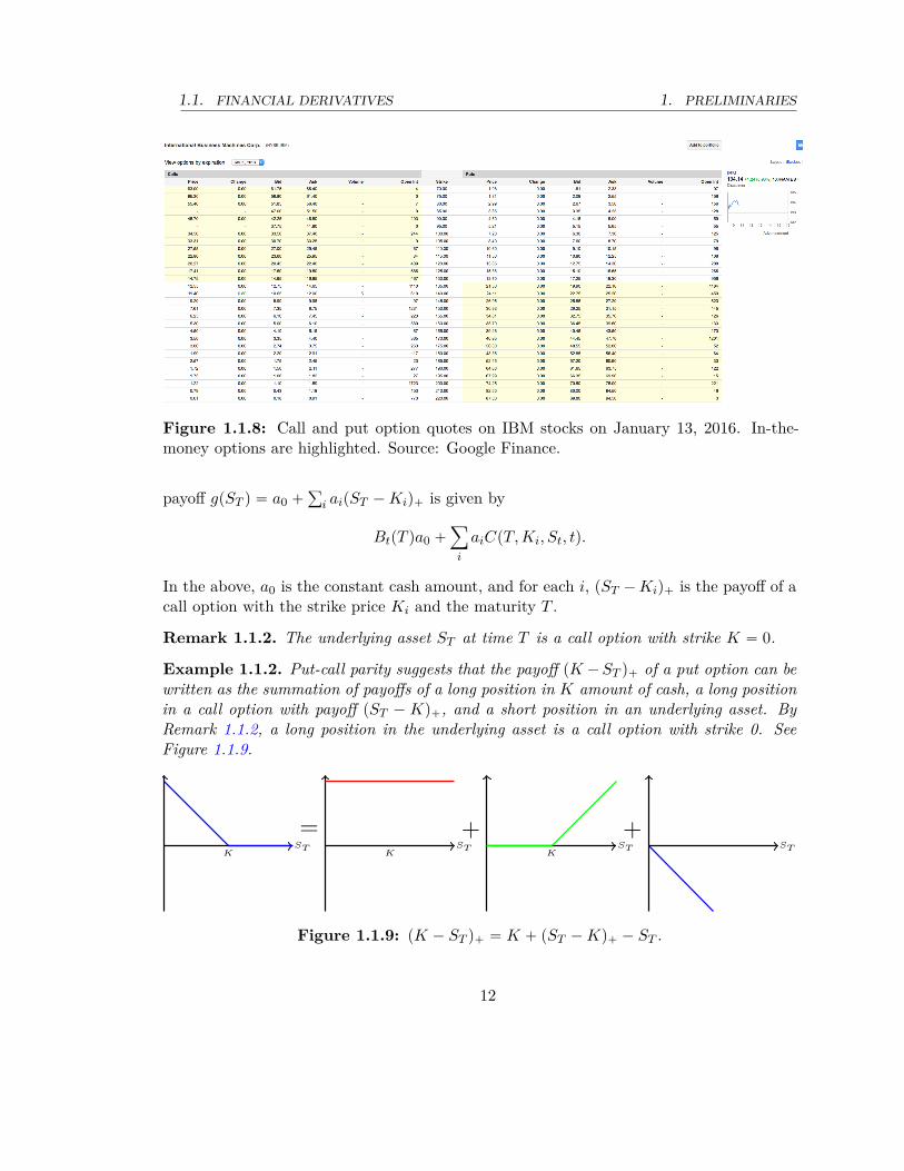
Figure 1.1.8: Call and put option quotes on IBM stocks on January 13, 2016. In-the-money options are highlighted. Source: Google Finance.
payoff gpST q “ a0 `ř
i aipST ´ Kiq` is given by
BtpT qa0 `ÿ
i
aiCpT, Ki, St, tq.
In the above, a0 is the constant cash amount, and for each i, pST ´ Kiq` is the payoff of acall option with the strike price Ki and the maturity T .
Remark 1.1.2. The underlying asset ST at time T is a call option with strike K “ 0.
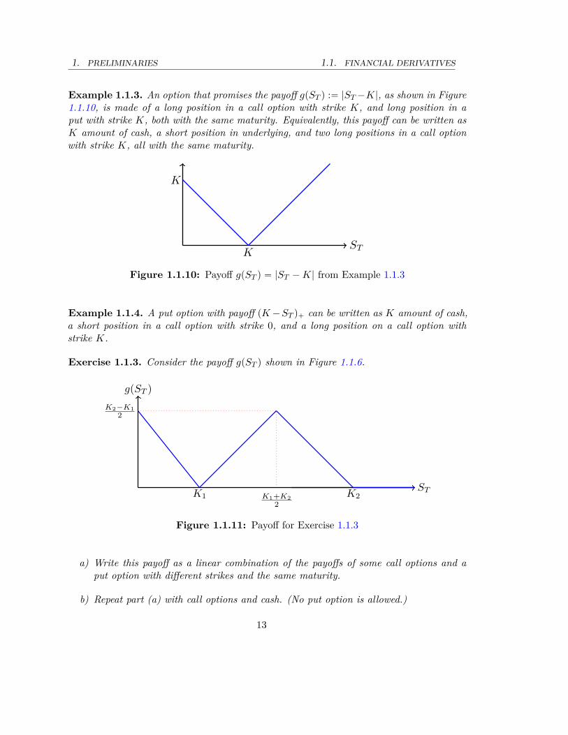
Example 1.1.2. Put-call parity suggests that the payoff pK ´ ST q` of a put option can bewritten as the summation of payoffs of a long position in K amount of cash, a long positionin a call option with payoff pST ´ Kq`, and a short position in an underlying asset. ByRemark 1.1.2, a long position in the underlying asset is a call option with strike 0. SeeFigure 1.1.9.
KST
=K
ST
+K
ST
+ST
Figure 1.1.9: pK ´ ST q` “ K ` pST ´ Kq` ´ ST .
12
1. PRELIMINARIES 1.1. FINANCIAL DERIVATIVES
Example 1.1.3. An option that promises the payoff gpST q :“ |ST ´K|, as shown in Figure1.1.10, is made of a long position in a call option with strike K, and long position in aput with strike K, both with the same maturity. Equivalently, this payoff can be written asK amount of cash, a short position in underlying, and two long positions in a call optionwith strike K, all with the same maturity.
K
K
ST
Figure 1.1.10: Payoff gpST q “ |ST ´ K| from Example 1.1.3
Example 1.1.4. A put option with payoff pK ´ ST q` can be written as K amount of cash,a short position in a call option with strike 0, and a long position on a call option withstrike K.
Exercise 1.1.3. Consider the payoff gpST q shown in Figure 1.1.6.
K1 K2K1+K2
2
K2−K1
2
ST
g(ST )
Figure 1.1.11: Payoff for Exercise 1.1.3
a) Write this payoff as a linear combination of the payoffs of some call options and aput option with different strikes and the same maturity.
b) Repeat part (a) with call options and cash. (No put option is allowed.)
13

1.1. FINANCIAL DERIVATIVES 1. PRELIMINARIES
1.1.4 American options
European options can only be exercised at a maturity for the payoff gpST q. An Americanoption gives its owner the right but not the obligation to exercise at any date before orat maturity. Therefore, at the time of exercise τ P r0, T s, an American call option has anexercise value equal to pSτ ´Kq`. We use the notation CAmpT, K, S, tq and PAmpT, K, S, tqto denote the price of an American call and an American put, respectively.The exercise time τ is not necessarily deterministic. More precisely, it can be a random
time that depends upon the occurrence of certain events in the market. An optimal exercisetime can be found among those of threshold type; the option is exercised before maturitythe first time the market price of option becomes equal to the exercise value, whereas theoption usually has a higher market value than the exercise value. Notice that both of thesequantities behave randomly over time.
1.1.5 Bond and forward rate agreements
A zero-coupon bond (or simply zero bond) is a fixed-income security that promises a fixedamount of cash in a specified currency at a certain time in the future, e.g., $100 on January30. The promised cash is called the principle, face value or par value and the time of deliveryis called the maturity. All bonds are traded in specialized markets at a price often lowerthan the principle3.For simplicity, throughout this book, a zero bond means a zero bond with principle of $1,
unless the principle is specified; for example, a zero bond with principle of $10 is ten zerobond s. At a time t, we denote the price of a zero bond maturing at T by BtpT q.We can use the price of a zero bond to calculate the present value of a future payment
or cashflow. For example, if an amount of $x at time T is worth xBtpT q
at an earlier timet. This is because, if we invest $ x
BtpT qin a zero bond with maturity T , at the maturity we
receive a dollar amount of xBtpT q
BtpT q “ x.The price of the zero bond is the main indicator of the interest rate. While the term
“interest rate” is used frequently in news and daily conversations, the precise definitionof the interest rate depends on the time horizon and the frequency of compounding. Aninterest rate compounded yearly is simply related to the zero bond price by 1`R(yr) “ 1
B0p1q,
while for an interest rate compounded monthly, we have`
1 ` R(mo)
12˘12
“ 1B0p1q
. Therefore,
1 ` R(yr) “
´
1 `R(mo)
12
¯12.
Generally, an interest rate n times compounded during the time interval rt, T s, denotedby R
pnqt pT q, satisfies
´
1 `R
pnqt pT q
n
¯n“ 1
BtpT q. When the frequency of compounding n
3There have been instances when this has not held, e.g., the financial crisis of 2007.
14
1. PRELIMINARIES 1.1. FINANCIAL DERIVATIVES
approaches infinity, we obtainBtpT q “ e´R
p8qt pT q.
This motivates the definition of the zero-bond yield. The yield (or yield curve) RtpT q ofthe zero bond BtpT q is defined by
BtpT q “ e´pT ´tqRtpT q or RtpT q :“ ´1
T ´ tln BtpT q. (1.1.2)
The yield is a bivariate function R : pt, T q P D Ñ Rě0 where D is given by tpt, T q : T ą
0 and t ă T u. Yield is sometimes referred to as the term structure of the interest rate sinceboth variables t and T are time.If the yield curve is a constant, i.e., RtpT q “ r for all pt, T q P D, then, BtpT q “ e´rpT ´tq.
In this case, r is called the continuously compounded, instantaneous, spot, or short rate.However, the short rate does not need to be constant. A time-dependent short interestrate is a function r : r0, T s Ñ R` such that for any T ą 0, and t P r0, T s we haveBtpT q “ e´
şTt rsds; or equivalently, short rate can be defined as
rt :“ ´B ln BtpT q
BT
ˇ
ˇ
ˇ
T “t“
B ln BtpT q
Bt.
The short rate r or rs is an abstract concept; it exists because it is easier to model theshort rate than the yield curve. In practice, the interest rate is usually given by the yieldcurve.Besides zero bonds, there are other bonds that pay coupons on a regular basis, for example
a bond that pays the principle of $100 in 12 months and $20 every quarter. A coupon-carrying bond, or simply, a coupon bond, can often be described as a linear combinationof zero bonds; i.e., a bond with coupon payments of $ ci at date Ti with T1 ă ... ă Tn´1and principle payment P at maturity Tn “ T is the same as a portfolio of zero bonds withprinciple ci and maturity Ti for i “ 1, ..., n and is worth
n´1ÿ
i“1ciBtpTiq ` PBtpTnq “
n´1ÿ
i“1cie
´pTi´tqRtpTiq ` Pe´pTn´tqRtpTnq.
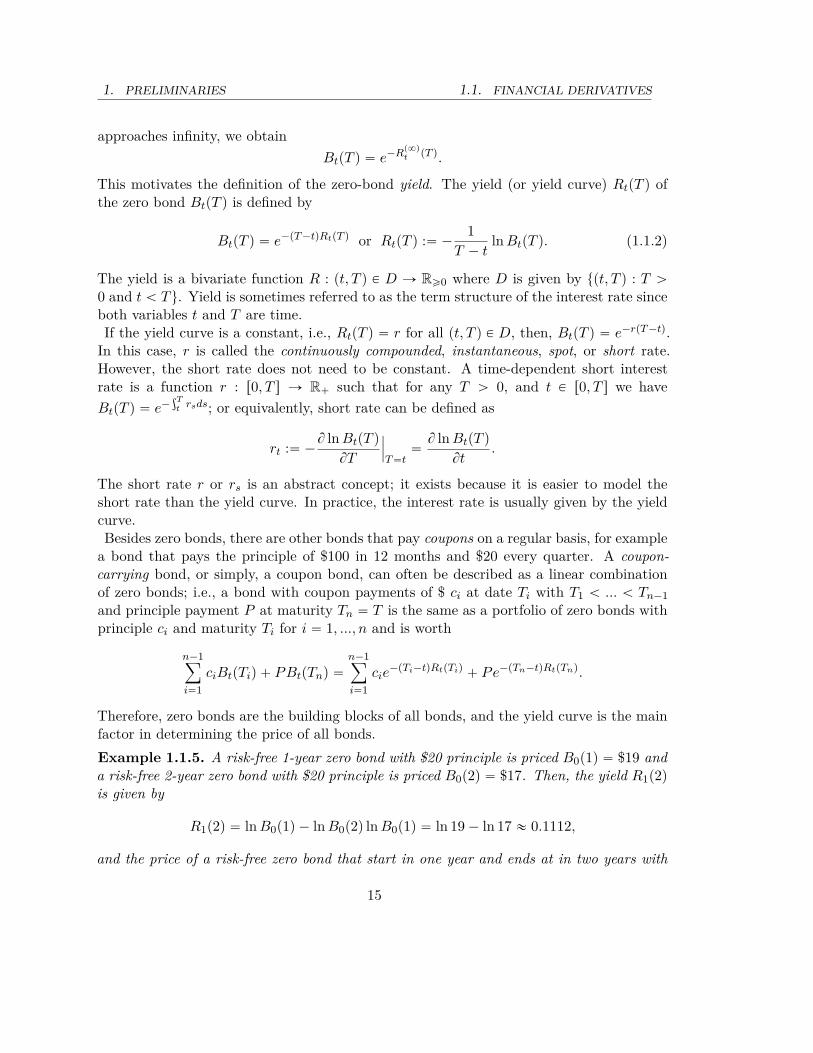
Therefore, zero bonds are the building blocks of all bonds, and the yield curve is the mainfactor in determining the price of all bonds.Example 1.1.5. A risk-free 1-year zero bond with $20 principle is priced B0p1q “ $19 anda risk-free 2-year zero bond with $20 principle is priced B0p2q “ $17. Then, the yield R1p2q
is given by
R1p2q “ ln B0p1q ´ ln B0p2q ln B0p1q “ ln 19 ´ ln 17 « 0.1112,
and the price of a risk-free zero bond that start in one year and ends at in two years with
15
1.1. FINANCIAL DERIVATIVES 1. PRELIMINARIES
principle $20 is given by
B1p2q “ 100e´R1p2q “170019
« 89.47.
The price of a bond that pays a $30 coupon at the end of the current year and $100 as theprinciple in two years equals to
30B0p1q
100` 100B0p2q
100“ 5.9 ` 17 “ 22.9.
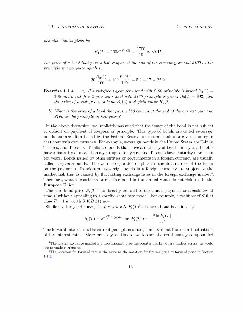
Exercise 1.1.4. a) If a risk-free 1-year zero bond with $100 principle is priced B0p1q “
$96 and a risk-free 2-year zero bond with $100 principle is priced B0p2q “ $92, findthe price of a risk-free zero bond B1p2q and yield curve R1p2q.
b) What is the price of a bond that pays a $30 coupon at the end of the current year and$100 as the principle in two years?
In the above discussion, we implicitly assumed that the issuer of the bond is not subjectto default on payment of coupons or principle. This type of bonds are called sovereignbonds and are often issued by the Federal Reserve or central bank of a given country inthat country’s own currency. For example, sovereign bonds in the United States are T-bills,T-notes, and T-bonds. T-bills are bonds that have a maturity of less than a year, T-noteshave a maturity of more than a year up to ten years, and T-bonds have maturity more thanten years. Bonds issued by other entities or governments in a foreign currency are usuallycalled corporate bonds. The word “corporate” emphasizes the default risk of the issueron the payments. In addition, sovereign bonds in a foreign currency are subject to themarket risk that is caused by fluctuating exchange rates in the foreign exchange market4.Therefore, what is considered a risk-free bond in the United States is not risk-free in theEuropean Union.The zero bond price BtpT q can directly be used to discount a payment or a cashflow at
time T without appealing to a specific short rate model. For example, a cashflow of $10 attime T “ 1 is worth $ 10B0p1q now.Similar to the yield curve, the forward rate FtpT q5 of a zero bond is defined by
BtpT q “ e´şTt Ftpuqdu or FtpT q :“ ´
B ln BtpT q
BT.
The forward rate reflects the current perception among traders about the future fluctuationsof the interest rates. More precisely, at time t, we foresee the continuously compounded
4The foreign exchange market is a decentralized over-the-counter market where traders across the worlduse to trade currencies.
5The notation for forward rate is the same as the notation for futures price or forward price in Section1.1.1.
16

1. PRELIMINARIES 1.1. FINANCIAL DERIVATIVES
interest rates for N time intervals rt0, t1s, rt1, t2s, ..., rtN´1, T s in the future as Ftptq,Ftpt1q, ..., FtptN´1q, respectively. Here, for n “ 0, ..., N , tn “ t ` nδ and δ “ T ´t
N .Then, $1 at time T is worth e´FtptN´1qδq at time tN´1, e´pFtptN´1q`FtptN´2qqδ at time tN´2,e´pFtptN´1q`...`Ftptnqqδ at time tn, and e´pFtptN´1q`...`Ftpt1q`Ftptqqδ at time t. As n goes toinfinity, the value BtpT q of the zero bond converges to
limnÑ8
e´řN´1
n“0 Ftptnqδ “ e´şTt Ftpuqdu.
The forward rates are related to so-called forward rate agreements. A forward rate agree-ment is a contract between two parties both committed to exchanging a specific loan (azero bond with a specified principle and a specific maturity) in a future time (called thedelivery date) with a specific interest rate. We can denote the agreed rate by fpt0, t, T q
where t0 is the current time, t is the delivery date, and T is the maturity of the bond. Asalways, we take principle to be $1. Then, the price of the underlying bond at time t shouldequal BtpT q “
Bt0 pT q
Bt0 ptq. This is because, if we invest $ x in Bt0ptq at time t0, we have x
Bt0 ptqat
time t. Then, at time t, we reinvest this amount in BtpT q. At time T , we have xBt0 ptqBtpT q
.Alternatively, if we invest in Bt0pT q from the beginning, we obtain x
Bt0 pT q, which must be
the same as the value of the two-step investment described above6. Therefore, the fairforward rate in a forward rate agreement must satisfy
ft0pt, T q “ ´ln Bt0pT q ´ ln Bt0ptq
T ´ t.
If we let T Ó t, we obtain limT Ót ft0pt, T q “ Ft0ptq. In terms of yield, we have
ft0pt, T q “pT ´ t0qRt0pT q ´ pt ´ t0qRt0ptq
T ´ t.
Ft0ptq is the instantaneous forward rate. However, ft0pt, T q is the forward rate at time t0for time interval rt, T s and is related to the instantaneous forward rate by
ft0pt, T q “
ż T
tFt0puqdu.
Unlike the forward rate and short rate rt, yield curve RtpT q is accessible through marketdata. For example, LIBOR7 is the rate at which banks worldwide agree to lend to each otherand is considered more or less a benchmark interest rate for international trade. Or, theUnited States treasury yield curve is considered a risk-free rate for domestic transactionswithin the United States. The quotes of yield curve RtpT q for LIBOR and the United
6A more rigorous argument is provided in Section 1.2 Example 1.2.27London Interbank Offered Rate
17
1.1. FINANCIAL DERIVATIVES 1. PRELIMINARIES
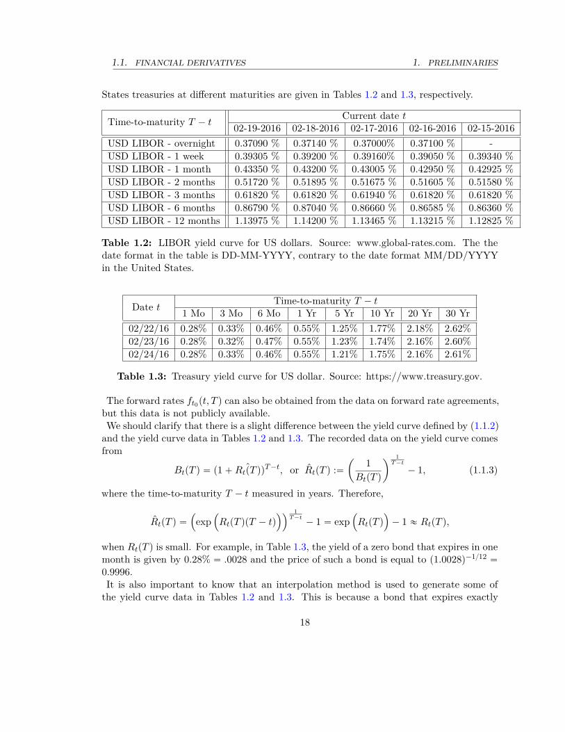
States treasuries at different maturities are given in Tables 1.2 and 1.3, respectively.
Time-to-maturity T ´ tCurrent date t
02-19-2016 02-18-2016 02-17-2016 02-16-2016 02-15-2016USD LIBOR - overnight 0.37090 % 0.37140 % 0.37000% 0.37100 % -USD LIBOR - 1 week 0.39305 % 0.39200 % 0.39160% 0.39050 % 0.39340 %USD LIBOR - 1 month 0.43350 % 0.43200 % 0.43005 % 0.42950 % 0.42925 %USD LIBOR - 2 months 0.51720 % 0.51895 % 0.51675 % 0.51605 % 0.51580 %USD LIBOR - 3 months 0.61820 % 0.61820 % 0.61940 % 0.61820 % 0.61820 %USD LIBOR - 6 months 0.86790 % 0.87040 % 0.86660 % 0.86585 % 0.86360 %USD LIBOR - 12 months 1.13975 % 1.14200 % 1.13465 % 1.13215 % 1.12825 %
Table 1.2: LIBOR yield curve for US dollars. Source: www.global-rates.com. The thedate format in the table is DD-MM-YYYY, contrary to the date format MM/DD/YYYYin the United States.
Date tTime-to-maturity T ´ t
1 Mo 3 Mo 6 Mo 1 Yr 5 Yr 10 Yr 20 Yr 30 Yr02/22/16 0.28% 0.33% 0.46% 0.55% 1.25% 1.77% 2.18% 2.62%02/23/16 0.28% 0.32% 0.47% 0.55% 1.23% 1.74% 2.16% 2.60%02/24/16 0.28% 0.33% 0.46% 0.55% 1.21% 1.75% 2.16% 2.61%
Table 1.3: Treasury yield curve for US dollar. Source: https://www.treasury.gov.
The forward rates ft0pt, T q can also be obtained from the data on forward rate agreements,but this data is not publicly available.We should clarify that there is a slight difference between the yield curve defined by (1.1.2)
and the yield curve data in Tables 1.2 and 1.3. The recorded data on the yield curve comesfrom
BtpT q “ p1 ` ˆRtpT qqT ´t, or RtpT q :“ˆ
1BtpT q
˙1
T ´t
´ 1, (1.1.3)
where the time-to-maturity T ´ t measured in years. Therefore,
RtpT q “
´
exp´
RtpT qpT ´ tq¯¯
1T ´t
´ 1 “ exp´
RtpT q
¯
´ 1 « RtpT q,
when RtpT q is small. For example, in Table 1.3, the yield of a zero bond that expires in onemonth is given by 0.28% “ .0028 and the price of such a bond is equal to p1.0028q´112 “
0.9996.It is also important to know that an interpolation method is used to generate some of
the yield curve data in Tables 1.2 and 1.3. This is because a bond that expires exactly
18

1. PRELIMINARIES 1.1. FINANCIAL DERIVATIVES
in one month, three months, six months, or some other time does not necessarily alwaysexist. A bond that expires in a month will be a three-week maturity bond after a week.Therefore, after calculating the yield for the available maturities, an interpolation givesus the interpolated yields of the standard maturities in the yield charts. For example, inTable 1.3, The Treasury Department uses the cubic Hermite spline method to generatedaily yield curve quotes.
Remark 1.1.3. While the market data on the yield of bonds with different maturity isprovided in the discrete-time sense, i.e., (1.1.3), the task of modeling a yield curve infinancial mathematics is often performed in continuous-time. Therefore, it is important tolearn both frameworks and the relation between them.
Sensitivity analysis of the bond price
We measure the sensitivity of the zero bond price with respect to changes in the yieldor errors in the estimation of the yields by dBtpT q
dRtpT q“ ´pT ´ tqBtpT q. As expected, the
sensitivity is negative, which means that the increase (decrease) in yield is detrimental(beneficial) to the bond price. It is also proportional to the time-to-maturity of the bond;i.e., the duration of the zero bond is equal to ´
dBtpT qdRtpT q
BtpT q. For a coupon bond, the
sensitivity is measured after defining the yield of the bond; the yield of a coupon bondwith coupons payments of $ ci at date Ti with T1 ă ... ă Tn´1 and principle paymentP “ cn at maturity Tn “ T is a number y such that ppyq equals the price of the bond, andppyq is the function defined below:
ppyq :“nÿ
i“1cie
´pTi´tqy.
Therefore, the yield of a bond is the number y that satisfiesnÿ
i“1cie
´pTi´tqy “
nÿ
i“1ciBtpTiq.
The function ppyq is a strictly decreasing function with pp´8q “ 8, pp0q “řn´1
i“1 ci ` P ,and pp8q “ 0. Therefore, for a bond with a positive price, the yield of the bond exists asa real number. In addition, if the price of the bond is in the range p0, pp0qq, the yield ofthe bond is a positive number.Therefore, the yield y depends on all parameters t, ci, Ti, and RtpTiq, for i “ 1, ..., n.
Motivated from the zero bond, the duration the coupon bond is given by
D :“ ´dpdy
ppyq “
nÿ
i“1pTi ´ tq
cie´pTi´tqy
ppyq,
19
1.1. FINANCIAL DERIVATIVES 1. PRELIMINARIES
a naturally weighted average of the duration of payments, with weights cie´pTi´tqy
ppyq, for
i “ 1, ..., n.The convexity of a zero bond is defined by using the second derivative C :“ d2BtpT qdRtpT q2
BtpT q“
pT ´ tq2, and for a coupon bond is expressed as
C :“ d2pdy2
ppyq “
nÿ
i“1pTi ´ tq2 cie
´pTi´tqy
ppyq.
Recall that a function f is convex if and only if fpλx ` p1 ´ λqyq ď
λfpxq ` p1 ´ λqfpyq for all λ P p0, 1q. If the function is twice dif-ferentiable, convexity is equivalent to f2 ě 0. For more details onconvexity, see Section A.1.
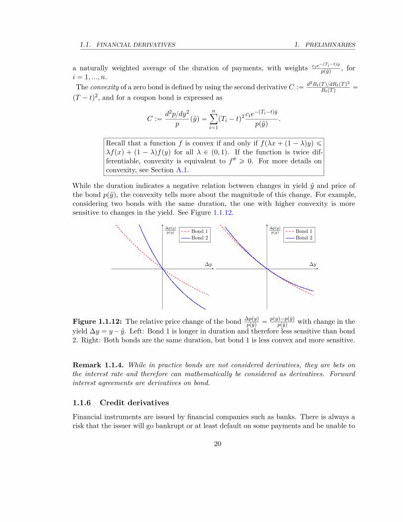
While the duration indicates a negative relation between changes in yield y and price ofthe bond ppyq, the convexity tells more about the magnitude of this change. For example,considering two bonds with the same duration, the one with higher convexity is moresensitive to changes in the yield. See Figure 1.1.12.
∆y
∆p(y)p(y) Bond 1
Bond 2
∆y
∆p(y)p(y) Bond 1
Bond 2
Figure 1.1.12: The relative price change of the bond ∆ppyq
ppyq“
ppyq´ppyq
ppyqwith change in the
yield ∆y “ y ´ y. Left: Bond 1 is longer in duration and therefore less sensitive than bond2. Right: Both bonds are the same duration, but bond 1 is less convex and more sensitive.
Remark 1.1.4. While in practice bonds are not considered derivatives, they are bets onthe interest rate and therefore can mathematically be considered as derivatives. Forwardinterest agreements are derivatives on bond.
1.1.6 Credit derivatives
Financial instruments are issued by financial companies such as banks. There is always arisk that the issuer will go bankrupt or at least default on some payments and be unable to
20
1. PRELIMINARIES 1.1. FINANCIAL DERIVATIVES
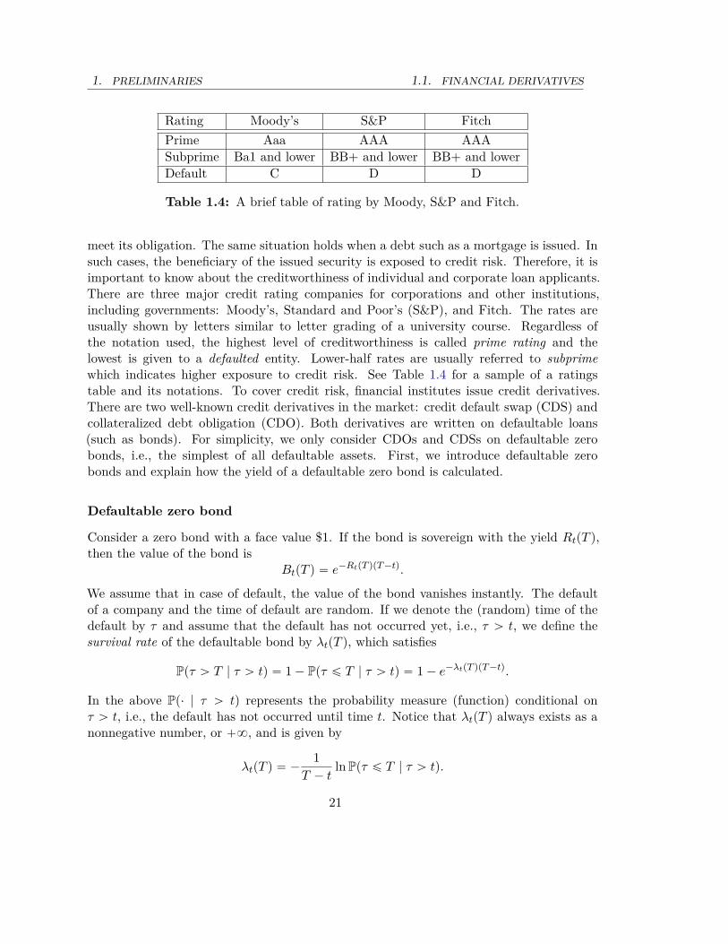
Rating Moody’s S&P FitchPrime Aaa AAA AAASubprime Ba1 and lower BB+ and lower BB+ and lowerDefault C D D
Table 1.4: A brief table of rating by Moody, S&P and Fitch.
meet its obligation. The same situation holds when a debt such as a mortgage is issued. Insuch cases, the beneficiary of the issued security is exposed to credit risk. Therefore, it isimportant to know about the creditworthiness of individual and corporate loan applicants.There are three major credit rating companies for corporations and other institutions,including governments: Moody’s, Standard and Poor’s (S&P), and Fitch. The rates areusually shown by letters similar to letter grading of a university course. Regardless ofthe notation used, the highest level of creditworthiness is called prime rating and thelowest is given to a defaulted entity. Lower-half rates are usually referred to subprimewhich indicates higher exposure to credit risk. See Table 1.4 for a sample of a ratingstable and its notations. To cover credit risk, financial institutes issue credit derivatives.There are two well-known credit derivatives in the market: credit default swap (CDS) andcollateralized debt obligation (CDO). Both derivatives are written on defaultable loans(such as bonds). For simplicity, we only consider CDOs and CDSs on defaultable zerobonds, i.e., the simplest of all defaultable assets. First, we introduce defaultable zerobonds and explain how the yield of a defaultable zero bond is calculated.
Defaultable zero bond
Consider a zero bond with a face value $1. If the bond is sovereign with the yield RtpT q,then the value of the bond is
BtpT q “ e´RtpT qpT ´tq.
We assume that in case of default, the value of the bond vanishes instantly. The defaultof a company and the time of default are random. If we denote the (random) time of thedefault by τ and assume that the default has not occurred yet, i.e., τ ą t, we define thesurvival rate of the defaultable bond by λtpT q, which satisfies
Ppτ ą T | τ ą tq “ 1 ´ Ppτ ď T | τ ą tq “ 1 ´ e´λtpT qpT ´tq.
In the above Pp¨ | τ ą tq represents the probability measure (function) conditional onτ ą t, i.e., the default has not occurred until time t. Notice that λtpT q always exists as anonnegative number, or `8, and is given by
λtpT q “ ´1
T ´ tlnPpτ ď T | τ ą tq.
21
1.1. FINANCIAL DERIVATIVES 1. PRELIMINARIES
If λtpT q “ 0, the bond is sovereign and never defaults. Otherwise, if λtpT q “ `8, theprobability of default is 1 and the default is a certain event. The payoff of a defaultablebond is given by the indicator random variable below:
1tτąT u :“
#
1 when τ ą T,
0 when τ ď T.
A common formalism in pricing financial securities with a random payoff is to take expecta-tion from the discounted payoff. More precisely, the value of the defaultable bond is givenby the expected value of the discounted payoff, i.e.,
Bλt pT q :“ E
“
BtpT q1tτąT u | τ ą t‰
“ BtpT qPpτ ą T | τ ą tq “ e´RtpT qpT ´tq´
1´e´λtpT qpT ´tq¯
.
The risk-adjusted yield of a defaultable bond is defined by the value Rλt pT q such that
e´Rλt pT qpT ´tq “ Bλ
t pT q “ e´RtpT qpT ´tq´
1 ´ e´λtpT qpT ´tq¯
.
Equivalently,Rλ
t pT q “ RtpT q ´1
T ´ tln´
1 ´ e´λtpT qpT ´tq¯
For a defaultable bond, we always have Rλt pT q ą RtpT q. Notice that when λtpT q Ò 8,
Rλt pT q Ó RtpT q, and when λtpT q Ó 0, Rλ
t pT q Ò 8. .
The higher the probability of default, the higher the adjusted yield ofthe bond.
Exercise 1.1.5. Consider a defaultable zero bond with T “ 1, face value $1, and survivalrate 0.5. If the current risk-free yield for maturity T “ 1 is 0.2, find the adjusted yield ofthis bond.
Credit default swap (CDS)
A CDS is a swap that protects the holder of a defaultable asset against default before acertain maturity time T by recovering a percentage of the nominal value specified in thecontract in case the default happens before maturity. Usually, some percentage of theloss can be covered by collateral or other assets of the defaulted party, i.e., a recoveryrate denoted by R. The recovery rate R is normally a percentage of the face value of thedefaultable bond and is evaluated prior to the time of issue. Therefore, the CDS covers1 ´ R percent of the value of the asset at the time of default. In return, the holder makesregular, constant premium payments κ until the time of default or maturity, whicheverhappens first. The maturity of a CDS is often the same as the maturity of the defaultable
22

1. PRELIMINARIES 1.1. FINANCIAL DERIVATIVES
asset, if there is any. For example, a CDS on a bond with maturity T also expires at timeT .
To find out the fair premium payments κ for the CDS, let’s denote the time of the defaultby τ and the face value of the defaultable bond by P . If the default happens at τ ď T , theCDS pays the holder an amount of p1 ´ RqP . The present value of this amount is obtainedby discounting it with a sovereign zero bond, i.e., p1 ´ RqPB0pT ^ τq. If the issuer of thebond defaults after time T , the CDS does not pay any amount. Thus, the payment of theCDS is a random variable expressed as
p1 ´ RqPB0pT ^ τq1tτďT u.
The holder of the CDS makes regular payments of amount κ at times 0 “ T0 ă T1 ă ¨ ¨ ¨ ă
Tn with Tn ă T . Then, the present value of payment of amount κ, paid at time Ti is
κ1tTiăτuB0pTiq.
The total number of premium payments is N :“ maxti ` 1 : Ti ă τ ^ T u, which is alsoa random variable with values 1, ..., n ` 1. Therefore, the present value of all premiumpayments is given by
κNÿ
i“1B0pTiq.
The discounted payoff of the CDS starting at time t is given by
p1 ´ RqPB0pT ^ τq1tτďT u ´ κNÿ
i“1B0pTiq (1.1.4)
The only source of randomness in the above payoff is the default time, i.e., τ . This makesthe terms B0pT ^ τq1tτďT u and
řNi“1 B0pTiq random variables. Notice that, although each
individual term in the summationřN
i“1 B0pTiq is not random, the number of terms N inthe summation is.
Because of the presence of randomness, we follow the formalism that evaluates the priceof an asset with random payoff by taking the expected value of the discounted payoff. Incase of a CDS, the price is known to be zero; either party in a CDS does not pay or receiveany amount by entering a CDS contract. Therefore, the premium payments κ should besuch that the expected value of the payoff (1.1.4) vanishes. To do so, first we need to knowthe probability distribution of the time of default. The task of finding the distribution ofdefault can be performed through modeling the survival rate, which is defined in Section1.1.6. Provided that the distribution of default is known, κ can be determined by taking
23

1.1. FINANCIAL DERIVATIVES 1. PRELIMINARIES
the expected value as follows:
κ “ p1 ´ RqPE“
B0pT ^ τq1tτďT u
‰
E“ř
0ďTiăτ B0pTiq‰ . (1.1.5)
Exercise 1.1.6. Consider a CDS on a defaultable bond with maturity T “ 1 year andrecovery rate R at 90%. Let the default time τ be a random variable with the Poissondistribution with mean 6 months. Assume that the yield of a risk-free zero bond is a constant1 for all maturities within a year. Find the monthly premium payments of the CDS in termsof the principle of the defaultable bond P “ $1.
Collateralized debt obligation (CDO)
A CDO is a complicated financial instrument. For illustrative porpuses, we present a sim-plified structure of a CDO in this section. One leg of CDO is a special-purpose entity(SPE) that holds a portfolio of defaultable assets such as mortgage-backed securities, com-mercial real estate bonds, and corporate loans. These defaultable assets serve as collateral;therefore we call the portfolio of these assets a collateral portfolio. Then, SPE issues bonds,which pay the cashflow of the assets to investors in these bonds. The holders of thesespecial bonds do not uniformly receive the cashflow. There are four types of bonds in fourtrenches: senior, mezzanine, junior and equity. The cashflow is distributed among investorsfirst to the holders of senior bonds, then mezzanine bond holders, then junior bond holders,and finally equity bond holders. In case of default of some of the collateral assets in theportfolio, equity holders are the first to lose income. Therefore, a senior trench bond is themost expensive and an equity trench bond is the cheapest. CDOs are traded in specializeddebt markets, derivative markets, or over-the-counter (OTC).A CDO can be structurally very complicated. For illustration purpose, in the next example
we focus on a CDO that is written only on zero bonds.
Example 1.1.6. Consider a collateral portfolio of 100 different defaultable zero bondswith the same maturity. Let’s trenchize the CDO in four equally sized trenches as shownin Figure 1.1.13. If none of the bonds in the collateral portfolio default, the total $100cashflow will be evenly distributed among CDO bond holders. However, if ten bonds default,then total cashflow is $90; an amount of $75 to be evenly distributed among the junior,mezzanine, and senior holders, and the remaining amount of $15 dollars will be evenlydistributed among equity holders. If 30 bonds default, then total cashflow is $70; an amountof $50 to be evenly distributed among the mezzanine and senior holders, and the remainingamount of $5 dollars will be evenly distributed among mezzanine holders. Equity holdersreceive $0. If there are at least 50 defaults, equity and junior holders receive nothing. Themezzanine trench loses cashflow, if and only if the number of defaults exceed 50. The seniortrench receives full payment, if and only if the number of defaults remains at 75 or below.
24

1. PRELIMINARIES 1.1. FINANCIAL DERIVATIVES
equity
junior
mezzanine
senior
#ofdefaults
0
25
50
75
100
% of loss%100
Figure 1.1.13: Simplification of CDO structure
Above 75 defaults, equity, junior, and mezzanine trenches totally lose their cashflow, andsenior trench experiences a partial loss.
Exercise 1.1.7. Consider a credit derivative on two independently defaultable zero bondswith the same face value at the same maturity, which pays the face value of either bond incase of default of that bond. A credit derivative of this type is written on two independentlybonds: one of the bonds has a risk-adjusted yield of 5% and the other has a risk-adjustedyield of 15%. Another credit derivative of this type is written on two other independentlydefaulted bonds, both with a risk-adjusted yield of 10%. If both credit derivatives are offeredat the same price, which one is better? Hint: The probability of default is Ppτ ď T | τ ą tq “
e´λtpT qpT ´tq and the risk-adjusted yield satisfies Rλt pT q “ RtpT q ´ 1
T ´t ln´
1´e´λtpT qpT ´tq¯
.
Therefore, the probability of default satisfies Ppτ ď T | τ ą tq “ 1 ´ e´pRλt pT q´RtpT qqpT ´tq.
Loss distribution and systemic risk
We learned from the 2007 financial crisis that even a senior trench bond of a CDO can yieldyield an unexpectedly low cashflow caused by an unexpectedly large number of defaults inthe collateral portfolio, especially when the structure of the collateral portfolio creates asystemic risk. To explain the systemic risk, consider a collateral portfolio, which is madeup of mortgages and mortgage-based securities. These assets are linked through several
25

1.1. FINANCIAL DERIVATIVES 1. PRELIMINARIES
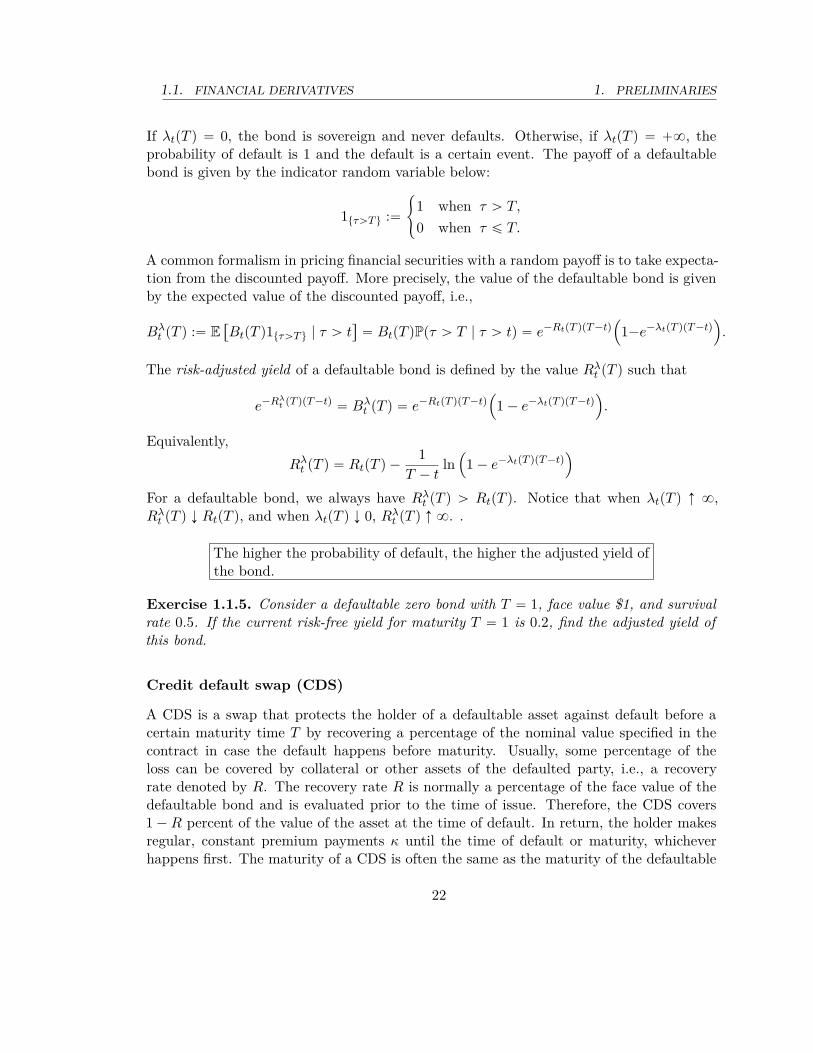
common risk factors, some are related to the real estate market, and the others are relatedto the overall situation of the economy. These risk factors create a correlation betweendefaults of these assets. Most of the risk factor that were known before the 2007 financialcrisis can only cause a relatively small group of assets within the collateral portfolio todefault. If risk factor can significantly increase the chance of default of a large group ofassets within the collateral portfolio, then it is a systemic risk factor. If we only look at thecorrelation between the defaults of the assets in the collateral portfolio, we can handle thenonsystemic risk factors. However, a systemic risk factor can only be found by studyingthe structure of the collateral portfolio beyond the correlation between the defaults.A difference between systemic and nonsystemic risk can be illustrated by the severity of
loss. In Figure 1.1.14, we show the distribution of loss in three different cases: independentdefaultable assets, dependent defaultable assets without a systemic factor, and dependentdefaultable assets with systemic factor. The loss distribution, when a systemic risk factorexists has at least one spike at a large loss level. It is important to emphasize that theempirical distribution of loss does not show the above-mentioned spike and the systemicrisk factor does not leave a trace in a calm situation of a market. Relying on only a period ofmarket data, in which systemic losses have not occurred, leads us into a dangerous territory,such as the financial meltdown of 2007–2008. Even having the data from a systemic eventmay not help predict the next systemic event, unless we have a sound understanding of thefinancial environment. Therefore, we can only find systemic risk factors through studyingthe structure of a market.Take the following example, as extreme and hypothetical as it is, as an illustration of
systemic risk. Consider a CDO made up of a thousand derivatives on a single defaultableasset. If the asset does not default, all trenches collect even shares of the payoff of thederivatives. However, in case of default, all trenches become worthless. Even if you increasethe number of assets to, ten, it only takes a few simultaneously defaulted assets to blow upthe CDO. Even when the number of assets becomes large, their default may only dependon few factors; i.e., when a few things go wrong, the CDO can become worthless.
Exercise 1.1.8. Consider a portfolio of 1000 defaultable asset with the same future value$1. Let Zi represent the loss from asset i which is 1 when asset i defaults and 0 otherwise.Therefore, the total loss of the portfolio is equal to L :“
ř1000i“1 Zi. Plot the probability
density function (pdf) of L in the following three cases.
a) Z1, ..., Z1000 are i.i.d. Bernoulli random variables with probability p “ .01.
b) Z1, ..., Z1000 are correlated in the following way. Given the number of defaults N ě 0,the defaulted assets can with equal likelihood be any combination of N out of 100assets, and N is distributed as a negative binomial with parameters pr, pq “ p90, .1q.When N ě 1000, all assets have defaulted. See Example B.14. Plot the pdf of L.
c) Now let X be a Bernoulli random variable with probability p “ .005. Given X “ 0,the new set of random variables Z1, ..., Z1000 are i.i.d. Bernoulli random variables
26
1. PRELIMINARIES 1.1. FINANCIAL DERIVATIVES
0 20 40 60 80 100
.05
.1
.15
SpikeyFat taily
Severity of total loss
UncorrelatedCorrelated
Correlated with systemic risk
22 24 26 28 30
.01
.02·10−2
Spike
y
Fat tail
y
Fat tail of correlated losses
UncorrelatedCorrelated
Figure 1.1.14: Distribution of loss: Correlation increases the probability at the tail of thedistribution of loss. Systemic risk adds a spike to the loss distribution. All distributionshave the same mean. The fat-tailed loss distribution and the systemic risk loss distributionhave the same correlation of default.
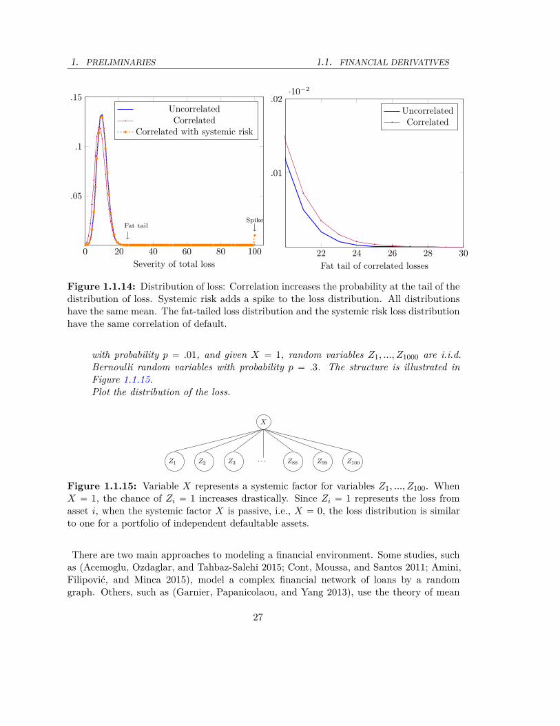
with probability p “ .01, and given X “ 1, random variables Z1, ..., Z1000 are i.i.d.Bernoulli random variables with probability p “ .3. The structure is illustrated inFigure 1.1.15.Plot the distribution of the loss.
X
Z1 Z2 Z3 · · · Z88 Z99 Z100
Figure 1.1.15: Variable X represents a systemic factor for variables Z1, ..., Z100. WhenX “ 1, the chance of Zi “ 1 increases drastically. Since Zi “ 1 represents the loss fromasset i, when the systemic factor X is passive, i.e., X “ 0, the loss distribution is similarto one for a portfolio of independent defaultable assets.
There are two main approaches to modeling a financial environment. Some studies, suchas (Acemoglu, Ozdaglar, and Tahbaz-Salehi 2015; Cont, Moussa, and Santos 2011; Amini,Filipović, and Minca 2015), model a complex financial network of loans by a randomgraph. Others, such as (Garnier, Papanicolaou, and Yang 2013), use the theory of mean
27

1.1. FINANCIAL DERIVATIVES 1. PRELIMINARIES
field games to model the structure of a financial environment. While the former emphasizesthe contribution of the heterogeneity of the network in systemic risk, the latter shows thatsystemic risk can also happen in a homogeneous environment. An example of such anetwork method, that most central banks and central clearinghouses use to assess systemicrisk to the financial networks they oversee is the Eisenberg-Noe model, which is discussedin Section 1.1.2.
1.1.7 Optimization in finance
Optimization is a regular practice in finance: a hedge fund wants to increase its profit,a retirement fund wants to increase its long-term capital gain, a public company wantsto increase its share value, and so on. One of the early applications of optimization infinance is the Markowitz mean-variance analysis on diversification; [23]. This leads toquadratic programming and linear optimization with quadratic constraint. Once we definethe condition for the optimality of a portfolio in a reasonable sense, we can build an optimalportfolio, or an efficient portfolio. Then, the efficient portfolio can be used to analyzeother investment strategies or price new assets. For example, in the capital asset pricingmodel (CAPM), we evaluate an asset based on its correlation with the efficient market. Inthis section, we present a mean-variance portfolio selection problem as a classical use ofoptimization methods in finance.Consider a market with N assets. Assume that we measure the profit of the asset over a
period r0, 1s by its return:
Ri “S
piq1 ´ S
piq0
Spiq0
.
Here, Spiq0 and S
piq1 are the current price and the future price of the asset i, respectively.
The return on an asset is the relative gain of the asset. For instance, if the price of an assetincreases by 10%, the return is 0.1. Since the future price is unknown, we take return as arandom variable and define the expected return by the expected value of the return, i.e.,
Ri :“ ErRis.
The risk of an asset is defined as the standard deviation of the return σi, where
σ2i :“ varpRiq.
Expected return and risk are two important factors in investment decisions. An investorwith a fixed amount of money wants to distribute her wealth over different assets to makean investment portfolio. In other words, she wants to choose weights pθ1, ..., θN q P RN
` suchthat
řNi“1 θi “ 1 and invest θi fraction of her wealth on asset i. Then, her expected return
28

1. PRELIMINARIES 1.1. FINANCIAL DERIVATIVES
on this portfolio choice is given by
Rθ :“Nÿ
i“1θiRi.
However, the risk of her portfolio is a little more complicated and depends on the correlationbetween the assets
σ2θ :“
Nÿ
i“1θ2
i σ2i ` 2
ÿ
1ďiăjďN
θiθjϱijσiσ2.
Here ϱij is the correlation between the returns of assets i and j.
Example 1.1.7 (Two assets). Assume that N “ 2 and R1 and R2 are assets with correlatedreturns, and that correlation is given by ϱ12. Thus, for θ P r0, 1s, we invest θ portion ofthe wealth in asset 1 and the rest in asset 2. Then, the expected return and the risk of theportfolio as a function of θ are given by
Rθ “ θR1 ` p1 ´ θqR2 and σ2θ “ θ2σ2
1 ` p1 ´ θq2σ22 ` 2θp1 ´ θqϱ12σ1σ2.
Therefore, by eliminating θ, σ2θ becomes a quadratic function of Rθ; see the red parabola in
Figure 1.1.16.
Exercise 1.1.9. Show that when θ “σ2
2σ2
1`σ22, the portfolio with two uncorrelated assets in
Example 1.1.7 takes the minimum risk σ2θ . Find the minimum value. Repeat the result for
the positively and negatively correlated assets.
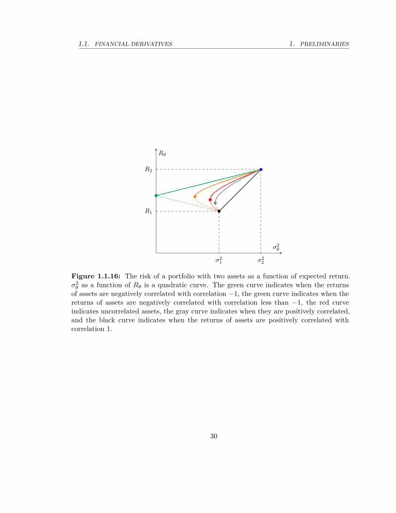
As seen in Figure 1.1.16 and shown in Exercise 1.1.9, there is a portfolio with minimumrisk σmin and return R˚ that is higher than the minimum return between the two assets. Ifthe goal is to minimize risk regardless of the return of the portfolio, there is a better optionthan fully investing in the lower-risk asset. Even if the assets are correlated, negatively orpositively, the minimum risk portfolio exists. The only exception is when the two assetsare positively correlated with ϱ12 “ 1, where the least risky option is to invest fully inthe asset with lower risk. Notice that in the dotted parts of the red and green curves, allportfolios are worse than the minimum risk portfolio. In other words, the minimum riskportfolio has higher return than all dotted portfolios while it maintains the lowest risk. Bychoosing a portfolio in the solid part of the curve, we accept to take higher risk than theminimum risk portfolio. In return, the return of the chosen portfolio also is higher thanthe return of the minimum risk portfolio. The solid part of the curve is called the efficientfrontier.The collection of all portfolios made up of more than two assets is not represented simply
by a one-dimensional curve; such a portfolio is represented by a point in a two-dimensionalregion that is not always easy to find. However, Robert Merton in [24] shows that the
29
1.1. FINANCIAL DERIVATIVES 1. PRELIMINARIES
σ21 σ2
2
R1
R2
σ2θ
Rθ
Figure 1.1.16: The risk of a portfolio with two assets as a function of expected return.σ2
θ as a function of Rθ is a quadratic curve. The green curve indicates when the returnsof assets are negatively correlated with correlation ´1, the green curve indicates when thereturns of assets are negatively correlated with correlation less than ´1, the red curveindicates uncorrelated assets, the gray curve indicates when they are positively correlated,and the black curve indicates when the returns of assets are positively correlated withcorrelation 1.
30
1. PRELIMINARIES 1.1. FINANCIAL DERIVATIVES
Figure 1.1.17: Left: the risk vs return of all portfolios on three assets. The assets aremarked by blue dots. The bi-asset risk-return curves are plotted with blue, green and redcolors. Right: The efficient frontier for three assets is shown in orange.
efficient frontier always exists regardless of the number of assets. In Figure 1.1.17, wesketched the risk-return region for three assets and marked the efficient frontier for them.To define the efficient frontier, we impose a natural partial order among all portfolios
based on their risk and return: θ ą θ if and only if Rθ ą Rθ and σθ ď σθ, or Rθ ě Rθ andσθ ă σθ. In other words, one portfolio is better than another if it has either a lower riskwith at least the same return, or a higher return with at most the same risk. The efficientfrontier is the set of all maximal portfolios under this order; i.e., there is no portfolio thatis better.
Minimum risk portfolio
The portfolio with the least risk σmin is located in the lowest end of the efficient frontier.To find the lowest-risk portfolio, we solve the following problem.
min σθ subject to θ ě 0 andÿ
i
θi “ 1.
Notice that the above optimization problem is equivalent to solving the quadratic program-ming problem.
min σ2θ subject to θ ě 0 and
ÿ
i
θi “ 1. (1.1.6)
Recall that
σ2θ :“
Nÿ
i“1θ2
i σ2i ` 2
ÿ
1ďiăjďN
θiθjϱijσiσ2
which can be written in matrix form by θTCθ. Here, the matrix C is the variance-covariancematrix between assets given by
Cij “ ϱijσiσj .
31

1.1. FINANCIAL DERIVATIVES 1. PRELIMINARIES
If all assets are linearly uncorrelated, then C is positive-definite. Therefore, problem (1.1.6)is similar to those studied in Section A.2.
Minimizing risk subject to return constraint
If we want to have a return higher than the return from the portfolio, we have to take morerisk than σmin. This can be achieved by adding the constraint of a minimum return.
min σθ subject to θ ě 0ÿ
i
θi “ 1 and Rθ ě R0. (1.1.7)
The constant R0 is the desired return from the portfolio.
Exercise 1.1.10. Consider a portfolio of ten assets with the expected return given by“
.1 .2 .3 .5 .2 .1 .05 .1 .2 .1‰
and the variance-covariance matrix by»
—
—
—
—
—
—
—
—
—
—
—
—
—
—
–
1 .2 0 0 0 0 0 0 0 0.2 1 .2 0 0 0 0 0 0 00 .2 1 .2 0 0 0 0 0 00 0 .2 1 .2 0 0 0 0 00 0 0 .2 2 .1 0 0 0 00 0 0 0 .1 2 .1 0 0 00 0 0 0 0 .1 2 .1 0 00 0 0 0 0 0 .1 2 .1 00 0 0 0 0 0 0 .1 2 .10 0 0 0 0 0 0 0 .1 2
fi
ffi
ffi
ffi
ffi
ffi
ffi
ffi
ffi
ffi
ffi
ffi
ffi
ffi
ffi
fl
Use CVX under MatLab or CVXOPT under Python, introduced in Section A.2, to numericallysolve problems (1.1.6) and (1.1.7).
Maximizing return subject to risk constraint
It is obvious that the highest return comes from the asset with the highest return. However,it may be too risky to invest all one’s resources in one risky asset. Therefore, there is usuallya risk constraint:
max Rθ subject to θ ě 0ÿ
i
θi “ 1 and σ2θ ď σ0. (1.1.8)
The constant σ0 is the maximum risk of the portfolio.
32

1. PRELIMINARIES1.2. NO-DOMINANCE PRINCIPLE AND MODEL-INDEPENDENT ARBITRAGE
Exercise 1.1.11. Assume that all assets are uncorrelated. Use the Cauchy-Schwartz in-equality to show that an optimal solution for problem (1.1.8) is obtained when θi “ Ri
aσ2i
where a “ř
iRi
σ2i.
Now consider the general case where the assets are correlated with a positive-definitevariance-covariance matrix. Use the Cholesky decomposition for the positive-definite ma-trices to find an optimal solution to the problem. Is the optimal solution unique?
1.2 No-dominance principle and model-independent arbitrageIn this section, we focus on the market properties that hold true objectively regardlessof the choice of the model. Therefore, here we do not make any assumption about thedynamics of the assets, the yield of zero bonds, and the like. Instead, we only impose twobasic assumptions and ignore any friction in the market such as transaction cost, liquidityrestriction, and nontradability of assets. Some of the contents of this section can be foundin [34, Section 1.2].We consider a sample space Ω that includes the collection of all possible events in the
market at future time T , and let χ be given set of portfolios (a collection of assets andstrategies on how to trade them dynamically) in the market. For any portfolio in χ, thepayoff of the portfolio is what it is worth at time T , and is a random variable from Ω to R.We assume that there exists a pricing function Π : χ Ñ R; i.e., the price of portfolio P isgiven by ΠpP q. We denote the payoff of portfolio P at the event ω P Ω by P pωq.The first assumption that we impose is the following:
Assumption 1.2.1 (No-dominance). If P P χ has a nonnegative payoff, i.e., P pωq ě 0for all ω P Ω, then the price ΠpP q of portfolio P is nonnegative.
Remark 1.2.1. No-dominance principle implies that two portfolios P1 and P2 with P1pωq “
P2pωq for all ω P Ω have the same price.
The second assumption is the linearity of the pricing function. For any two portfoliosP1 and P2, define P1 ‘ P2 is the portfolio made by combining the two. We impose thefollowing natural assumption of linearity.
Assumption 1.2.2. For P1, P2 P χ, we have
ΠpP1 ‘ P2q “ ΠpP1q ` ΠpP2q.
Let’s first fix some terminology that we’ll be using. By “being in a long position” in anasset, a bond, or the like, we mean that we hold the asset, bond, etc. Similarly, by “beingin a short position” in an asset, a bond, or the like, we mean that we owe the asset, bond,etc. For a bond or an option, the issuer is in the short position. Having a short positionin an asset means borrowing that asset and then selling it for cash or keeping it for other
33
1.2. MODEL-INDEPENDENT EVALUATION 1. PRELIMINARIES
reasons. This is often referred to as short selling, which is a common practice in the market.Usually, the borrower is obliged to pay the short-sold security back upon the request of thelender or in an agreed time.
Example 1.2.1. The forward price K satisfies
FtpT q “St
BtpT q.
To see this, consider a portfolio made of a long position in the underlying asset and ashort position in a “ FtpT q zero bonds at time t. The value of this portfolio at time T isST ´ FtpT q. This value is the same as the payoff of a long position in forward contract.Therefore, by the no-dominance principle (Remark 1.2.1), we obtain that the value of theportfolio is the same as the price of the forward contract, which is zero; St´BtpT qFtpT q “ 0.On the other hand, the price of the forward is zero and therefore we have the result.
Remark 1.2.2. Proposition 1.2.1 explains a market condition called contango in the fu-tures markets; the futures price is larger than the spot price. If holding an underlyingasset incurs storage cost, then the result of Proposition 1.2.1 may be violated and we haveFtpT q ă St. This market condition is called backwardation. Backwardation can also occurif the underlying of the futures contract is not even storable, for instance electricity.
Example 1.2.2. Forward rate f0pt, T q for delivery at time t of a zero bond with maturityT satisfies
f0pt, T q “ln B0ptq ´ ln B0pT q
T ´ t.
To see this, consider a portfolio made of a zero bond with a principle of $1 at time T . Theprice of this portfolio is B0pT q. On the other hand, consider another portfolio made of a for-ward rate agreement on a bond with the principle of $1 starting at time t, maturing at timeT , and with a forward rate f0pt, T q; and a bond with a principle of $e´f0pt,T qpT ´tq maturingat time t. The price of such a portfolio is $B0ptqe´f0pt,T qpT ´tq. Since both portfolios havethe same payoff of $1, they must have the same price. Thus, B0ptqe´f0pt,T qpT ´tq “ B0pT q.
Exercise 1.2.1. Consider a zero bond Bd0pT q in the domestic currency and another zero
bond Bf0pT q in a foreign currency. At the current time t “ 0, the domestic-to-foreign
exchange rate is denoted by rd/f0 , and the forward domestic-to-foreign exchange rate8 for
time T is denoted by fd/f0 pT q. Show that
Bd0pT qr
d/f0 “ Bf
0pT qfd/f0 pT q.
Proposition 1.2.1. The price of an American option is always greater than or equal tothe price of a European option with the same payoff.
8The forward exchange rate is guaranteed at maturity.
34
1. PRELIMINARIES 1.2. MODEL-INDEPENDENT EVALUATION
Proof. An American option can always be exercised, but not necessarily optimally, atmaturity, and generates the same payoff as a European option.
Proposition 1.2.2. The price of vanilla options satisfies
CpT, K1, S, tq ď CpT, K2, S, tq and P pT, K1, S, tq ě P pT, K2, S, tq,
where K1 ě K2.
Proof. Consider a portfolio that consists of a long position in a call option with strike priceK2 and a short position in a call option with strike K1, both maturing at T . Then, theterminal value of the portfolio is pST ´ K2q` ´ pST ´ K1q`, which is nonnegative. By theno-dominance principle, we have CpT, K2, S, tq ´ CpT, K1, S, tq ě 0. For a put options, asimilar argument works.
Exercise 1.2.2. Show that the price of an American call or put option is an increasingfunction of maturity T .
Exercise 1.2.3. Let λ P p0, 1q. Then,
CpT, λK1 ` p1 ´ λqK2, S, tq ď λCpT, K1, S, tq ` p1 ´ λqCpT, K2, S, tq.
In other words, the price of a call option is convex in K.Show the same claim for the price of a put option, an American call option, and an Amer-ican put option.
Exercise 1.2.4. It is well known that a convex function has right and left derivatives atall points. From the above exercise it follows that the right and the left derivatives of acall option price with respect to strike price, BK˘CpT, K, S, tq, exists. Use no-dominanceto show that
´BtpT q ď BK˘CpT, K, S, tq ď 0
Hint: Consider a portfolio made of a long position in a call with strike K2, a long positionin K2 ´ K1 bonds, and a short position in a call option with strike K1.
Proposition 1.2.3 (Put-call parity). The price of a call option and the price of a putoption with the same strike and maturity satisfy
CpT, K, S, tq ` KBtpT q “ S ` P pT, K, S, tq.
Proof. Since pST ´ Kq` ` K “ ST ` pK ´ ST q`, according to no-dominance principle, aportfolio consisting of a call option and K units of zero bond BtpT q is worth as much as aportfolio made of a put option and one unit of underlying asset.
35
1.2. MODEL-INDEPENDENT EVALUATION 1. PRELIMINARIES
Exercise 1.2.5. A portfolio of long positions in call options with the same maturity andstrikes on different assets is worth more than a call option on a portfolio of the same assetswith the same weight; i.e.,
nÿ
i“1λiCpT, Ki, Spiq, tq ě CpT, K, S, tq, (1.2.1)
where λi ě 0 is the number of units invested in the call option on the ith underlying asset,Ki ě 0 is the strike of the call option on the ith underlying asset , Spiq denotes the currentprice of the ith asset, K “
řni“1 λiKi, and S “
řni“1 λiS
piq is the value of a portfolio thathas λi units of ith asset for i “ 1, ..., n.
Remark 1.2.3. Exercise 1.2.5 demonstrates an important implication about the risk ofa portfolio. A portfolio made of different assets can be insured against the risk of priceincrease in two ways: by purchasing a call option for each unit of each asset or by purchasinga call option on the whole portfolio. It follows from (1.2.1) that the latter choice is cheaperthan the former. An option on a portfolio is called a basket option.
Proposition 1.2.4 (Arbitrage bounds for the price of a call option). The price of a calloption should satisfy
pS ´ BtpT qKq` ď CpT, K, S, tq ď S.
Proof. Since pST ´ Kq` ď ST , no-dominance implies that CpT, K, S, tq ď S. To see theright-hand side inequality, first notice that since 0 ď pST ´ Kq`, 0 ď CpT, K, S, tq. On theother hand, a portfolio of along position in the underlying asset and a short position in Kunits of zero bond has a payoff ST ´ K which is less than or equal to the payoff of calloption pST ´ Kq`. Therefore, S ´ KB0pT q ď CpT, K, S, tq. As a result, pS ´ BtpT qKq` “
maxt0, S ´ BtpT qKu ď CpT, K, S, tq.
The notion of model-specific arbitrage will later be explored in Section 1.3. However, inthis section, we present model-independent arbitrage, which is in the same context as theno-dominance principle.
Definition 1.2.1. A portfolio P with a positive payoff and a zero price is called a model-independent arbitrage. In other words, a portfolio P is called model-independent arbitrageif P pωq ą 0 for all ω P Ω, and ΠpP q “ 0.
By Definition 1.2.1, a portfolio with χpω1q “ 0 for some ω1 P Ω and P pωq ą 0 ω ‰ ω1 isnot a model-independent arbitrage. This leads to a weaker notion of arbitrage.
Definition 1.2.2. A portfolio P with a nonnegative payoff such that for some ω P ΩP pωq ą 0 and zero price is called a weak arbitrage. In other words, a portfolio P is calleda weak arbitrage if P pωq ě 0 for all ω P Ω, P pω1q ą 0 for some ω1 P Ω and ΠpP q “ 0.
36

1. PRELIMINARIES 1.2. MODEL-INDEPENDENT EVALUATION
Example 1.2.3. Let K1 ą K2 and CpT, K1, S, tq ą CpT, K2, S, tq. A portfolio that consistsof a short position in a call with strike K1, a long position in a call with strike K2, and thedifference ofCpT, K1, S, tq ´ CpT, K2, S, tq in cash is a model-independent arbitrage. Thisis because, the value of such a portfolio is zero. However, the payoff is pST ´ K2q ´ pST ´
K1q` ` CpT, K1, S, tq ´ CpT, K2, S, tq, which is strictly positive, and therefore we have amodel-independent arbitrage.On the other hand, if CpT, K1, S, tq “ CpT, K2, S, tq, the same portfolio described in the
previous paragraph has a positive value whenever ST ą K2, and a zero value otherwise.Therefore, it is only a weak arbitrage.
Example 1.2.4. As a result of Exercise 1.2.4, if the price of the option is smaller thatpS´BtpT qKq`, or larger than the asset price S, then there is a model-independent arbitrage.For example, if CpT, K, S, tq ą S, one can have a portfolio of a short position in a calland a long position in the underlying asset, and the difference CpT, K, S, tq ´ S in cash.The value of this portfolio is zero. However, the payoff is strictly positive, i.e., ST ´ pST ´
Kq` ` CpT, K, S, tq ´ S ą 0.
Remark 1.2.4. When CpT, K, S, tq “ S and K ą 0, Example 1.2.4 suggests that westill have a model-independent arbitrage, unless the event ST “ 0 is legitimate. Therefore,choice between the model-independent arbitrage or weak arbitrage depends on whether theevent ST “ 0 is included in Ω or not.
Proposition 1.2.5. If there is no model-independent arbitrage, then the no-dominanceprinciple holds.
Proof. Assume that no-dominance does not hold; i.e., there is a portfolio P with nonneg-ative payoff with a negative price ΠpP q. Then, consider a new portfolio made of a longposition in the old portfolio P and holding a zero bond with face value ´ΠpP q. The newportfolio has a positive payoff of P pωq ´ ΠpP q for each ω P Ω and a zero price. Therefore,it is a model-independent arbitrage.
Exercise 1.2.6. For 0 ă t ă T , show that if B0ptqBtpT q ą B0pT q (equiv. B0ptqBtpT q ă
B0pT q), there is a model-independent arbitrage.
Exercise 1.2.7. Consider a zero bond Bd0pT q on the domestic currency and another zero
bond Bf0pT q on a foreign currency. At the current time t “ 0, the domestic-to-foreign
exchange rate is denoted by rd/f0 and the forward domestic-to-foreign exchange rate for time
T is denoted by fd/f0 pT q. Show that if
Bd0pT qr
d/f0 ą Bf
0pT qfd/f0 pT q,
then there exists a model-independent arbitrage.
37
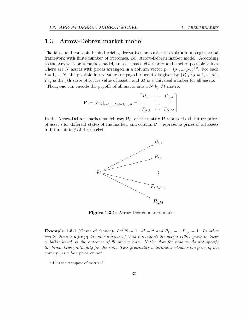
1.3. ARROW-DEBREU MARKET MODEL 1. PRELIMINARIES
1.3 Arrow-Debreu market model
The ideas and concepts behind pricing derivatives are easier to explain in a single-periodframework with finite number of outcomes, i.e., Arrow-Debreu market model. Accordingto the Arrow-Debreu market model, an asset has a given price and a set of possible values.There are N assets with prices arranged in a column vector p “ pp1, ..., pN qT9. For eachi “ 1, ..., N , the possible future values or payoff of asset i is given by tPi,j : j “ 1, ..., Mu.Pi,j is the jth state of future value of asset i and M is a universal number for all assets.Then, one can encode the payoffs of all assets into a N -by-M matrix
P :“ rPi,jsi“1,...,N,j“1,...,M “
»
—
–
P1,1 ¨ ¨ ¨ P1,M... . . . ...
PN,1 ¨ ¨ ¨ PN,M
fi
ffi
fl
.
In the Arrow-Debreu market model, row Pi,¨ of the matrix P represents all future pricesof asset i for different states of the market, and column P¨,j represents prices of all assetsin future state j of the market.
pi
Pi,1
Pi,2
...
Pi,M−1
Pi,M
Figure 1.3.1: Arrow-Debreu market model
Example 1.3.1 (Game of chance). Let N “ 1, M “ 2 and P1,1 “ ´P1,2 “ 1. In otherwords, there is a fee p1 to enter a game of chance in which the player either gains or losesa dollar based on the outcome of flipping a coin. Notice that for now we do not specifythe heads-tails probability for the coin. This probability determines whether the price of thegame p1 is a fair price or not.
9AT is the transpose of matrix A.
38

1. PRELIMINARIES 1.3. ARROW-DEBREU
p1
P1,1 = 1
P1,2 = −1
Figure 1.3.2: Game of chance described in the Arrow-Debreu market model
1.3.1 Arbitrage portfolio and the fundamental theorem of asset pricing
A portfolio is a row vector θ “ pθ1, ¨ ¨ ¨ , θN q where θi P R which represents the number ofunits of asset i in the portfolio. The total price of the portfolio is then given by
θp “
Nÿ
i“1θipi.
Here, the notation of product is simply the matrix product. Notice that if θi ą 0, theposition of the portfolio in asset i is called long, and otherwise if θi ă 0, it is called short.Arbitrage is a portfolio that costs no money but gives a nonnegative future value and for
some states positive values. More precisely, we have the following definition.
Definition 1.3.1. θ is called a weak arbitrage portfolio or weak arbitrage opportunity if
a) θp “ 0
b) θP¨,j ě 0 for all j “ 1, ..., M
c) θP¨,j ą 0 for at least one j.
Notice that for a given θ “ pθ1, ¨ ¨ ¨ , θN q, the portfolio represented by θ is itself an assetwith value θP¨j at the state j of the market.We say that a market model is free of weak arbitrage or that it satisfies no weak arbitrage
condition (NWA for short), if there is no weak arbitrage opportunity in this model.Sometimes, an arbitrage opportunity starts with a zero-valued portfolio and ends up with
positive values at all states of the market. This defined an strong arbitrage:
Definition 1.3.2. θ is called a strong arbitrage portfolio or arbitrage opportunity if
a) θp ă 0
b) θP¨,j ě 0 for all j “ 1, ..., M
Remark 1.3.1. Notice that if we remove some of the states of the market, then weakarbitrage can disappear. However, strong arbitrage does not.
39

1.3. ARROW-DEBREU 1. PRELIMINARIES
Notice that model-independent arbitrage as defined in Definition 1.2.1 is even strongerthan strong arbitrage.The following theorem is the most important in financial mathematics that characterizes
the notion of arbitrage in a simple way. Basically, it presents a simple criterion to determineif a market model is free of weak or strong arbitrage.
Theorem 1.3.1 (Fundamental theorem of asset pricing (FTAP)). The Arrow-Debreu mar-ket model is free of weak (respectively strong) arbitrage opportunity if and only if there exista column vector of positive (respectively nonnegative) numbers π “ pπ1, ..., πM qT such that
p “ Pπ. (1.3.1)
Notice that Theorem 1.3.1 does not claim that the vector π is unique, and therefore therecan be several solutions π such that (1.3.1) holds.
Proof. The proof for the strong arbitrage case is the result of the so-called Farkas’ lemmawhich asserts that
Given an n ˆ m matrix A and a vector b P Rm. Then, exactly one ofthe following two statements is true:
1) There exists a π P Rn such that Aπ “ b and π ě 0.
2) There exists a θ P Rm such that θA ě 0 and θb ă 0.
We apply Farkas’ lemma for A “ P and b “ p. Strong arbitrage is equivalent to (2) inFarkas’ lemma. Therefore, lack of strong arbitrage is equivalent to (1).To show the result for weak arbitrage, we consider the following extension of Farkas’s
lemma.
Given an n ˆ m matrix A and a vector b P Rm. Then, exactly one ofthe following two statements is true:
1’) There exists a π P Rn such that Aπ “ b and π ą 0.
2’) There exists a θ P Rm such that θA ě 0, θA ‰ 0 and θb ď 0.
For A “ P and b “ p, weak arbitrage is equivalent to (2’). Therefore, lack of weakarbitrage is equivalent to (1’).
Remark 1.3.2. The Farkas’ lemma and its extension that are used in the proof of Theorem1.3.1 are corollaries of the separating hyperplane theorem. For more details about separatinghyperplane theorem and Farkas’ lemma see [9, Section 5.8.3, Section 2.5.1 and Exercise2.20].
40
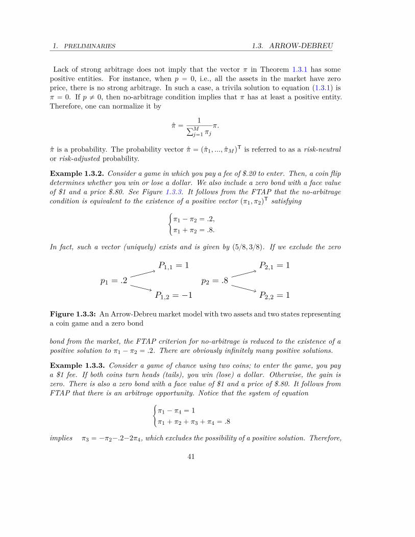
1. PRELIMINARIES 1.3. ARROW-DEBREU
Lack of strong arbitrage does not imply that the vector π in Theorem 1.3.1 has somepositive entities. For instance, when p “ 0, i.e., all the assets in the market have zeroprice, there is no strong arbitrage. In such a case, a trivila solution to equation (1.3.1) isπ “ 0. If p ‰ 0, then no-arbitrage condition implies that π has at least a positive entity.Therefore, one can normalize it by
π “1
řMj“1 πj
π.
π is a probability. The probability vector π “ pπ1, ..., πM qT is referred to as a risk-neutralor risk-adjusted probability.
Example 1.3.2. Consider a game in which you pay a fee of $.20 to enter. Then, a coin flipdetermines whether you win or lose a dollar. We also include a zero bond with a face valueof $1 and a price $.80. See Figure 1.3.3. It follows from the FTAP that the no-arbitragecondition is equivalent to the existence of a positive vector pπ1, π2qT satisfying
#
π1 ´ π2 “ .2,
π1 ` π2 “ .8.
In fact, such a vector (uniquely) exists and is given by p58, 38q. If we exclude the zero
p1 = .2
P1,1 = 1
P1,2 = −1
p2 = .8
P2,1 = 1
P2,2 = 1
Figure 1.3.3: An Arrow-Debreu market model with two assets and two states representinga coin game and a zero bond
bond from the market, the FTAP criterion for no-arbitrage is reduced to the existence of apositive solution to π1 ´ π2 “ .2. There are obviously infinitely many positive solutions.
Example 1.3.3. Consider a game of chance using two coins; to enter the game, you paya $1 fee. If both coins turn heads (tails), you win (lose) a dollar. Otherwise, the gain iszero. There is also a zero bond with a face value of $1 and a price of $.80. It follows fromFTAP that there is an arbitrage opportunity. Notice that the system of equation
#
π1 ´ π4 “ 1π1 ` π2 ` π3 ` π4 “ .8
implies π3 “ ´π2´.2´2π4, which excludes the possibility of a positive solution. Therefore,
41

1.3. ARROW-DEBREU 1. PRELIMINARIES
there is an arbitrage in this game.
p1 = 1
P1,1 = 1
P1,2 = 0
P1,3 = 0
P1,4 = −1
p2 = .8
P2,1 = 1
P2,2 = 1
P2,3 = 1
P2,4 = 1
Figure 1.3.4: An Arrow-Debreu market model with two assets and four states represent-ing a coin game and a zero bond
FTAP predicts the existence of arbitrage but does not provide any. Knowing an arbitrageopportunity exists, finding one is sometimes a challenging problem, even in the toy Arrow-Debreu market model.
Exercise 1.3.1. Find an arbitrage opportunity in Example 1.3.3.
Remark 1.3.3. The weak and strong arbitrage are model specific. If we change the model,the arbitrage opportunity can disappear. However, model-independent arbitrage remains astrong arbitrage opportunity in any possible model.
1.3.2 Arrow-Debreu market model with a risk-free bond
If we intend to add a new asset with price p1 and values P 11, ..., P 1
M to the current Arrow-Debreu market model, the new asset does not create an arbitrage opportunity if and onlyif at least one of the existing positive solutions π of (1.3.1) satisfies
p1 “
Mÿ
j“1P 1
jπj .
More specifically, assume that the new asset is a zero bond with yield (interest rate) Rand face value 1. Therefore, its price is given by p0 “ 1
1`R . See Figure 1.3.5. For no-arbitrage condition to hold for the market with the new bond, at least one of the positivesolutions of (1.3.1) implies that p0 “ 1
1`R “řM
j“1 πj . Therefore, no-arbitrage condition foran Arrow-Debreu market model with a zero bond is equivalent to existence of a positivevector π such that (1.3.1) holds and
Mÿ
j“1πj “
11 ` R
,
42
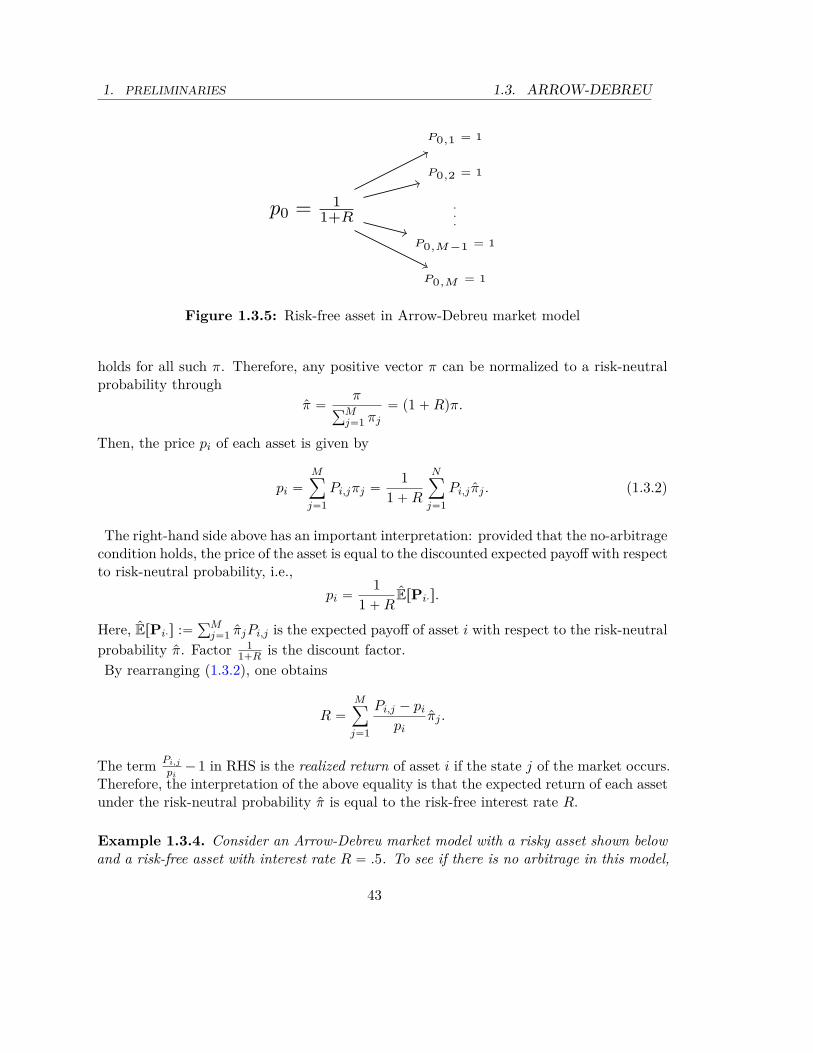
1. PRELIMINARIES 1.3. ARROW-DEBREU
p0 = 11+R
P0,1 = 1
P0,2 = 1
.
.
.
P0,M−1 = 1
P0,M = 1
Figure 1.3.5: Risk-free asset in Arrow-Debreu market model
holds for all such π. Therefore, any positive vector π can be normalized to a risk-neutralprobability through
π “π
řMj“1 πj
“ p1 ` Rqπ.
Then, the price pi of each asset is given by
pi “
Mÿ
j“1Pi,jπj “
11 ` R
Nÿ
j“1Pi,j πj . (1.3.2)
The right-hand side above has an important interpretation: provided that the no-arbitragecondition holds, the price of the asset is equal to the discounted expected payoff with respectto risk-neutral probability, i.e.,
pi “1
1 ` RErPi¨s.
Here, ErPi¨s :“řM
j“1 πjPi,j is the expected payoff of asset i with respect to the risk-neutralprobability π. Factor 1
1`R is the discount factor.By rearranging (1.3.2), one obtains
R “
Mÿ
j“1
Pi,j ´ pi
piπj .
The term Pi,j
pi´ 1 in RHS is the realized return of asset i if the state j of the market occurs.
Therefore, the interpretation of the above equality is that the expected return of each assetunder the risk-neutral probability π is equal to the risk-free interest rate R.
Example 1.3.4. Consider an Arrow-Debreu market model with a risky asset shown belowand a risk-free asset with interest rate R “ .5. To see if there is no arbitrage in this model,
43

1.3. ARROW-DEBREU 1. PRELIMINARIES
.3
1
.5
we should investigate the solutions to the system#
1 “ π1 ` π2
.3 “ 11.5 pπ1 ` .5π2q
The first equation accounts for that π is a probability vector, and the second equation comesfrom (1.3.2). However, the only solution is π “ p´.1, 1.1qT, which is not a probability.
Example 1.3.5. Consider an Arrow-Debreu market model with a risky asset shown belowand a risk-free asset with interest rate R “ .5. To see if there is no arbitrage in this model,
1
2
1
.5
we should investigate the solutions to the system
1 “ π1 ` π2 ` π3
1 “1
1.5p2π1 ` π2 ` .5π3q
One of the infinitely many solutions to the above system is π “ p.6, .2, .2qT, which impliesno-arbitrage condition.If a second risky asset, shown below, is added to the market, we still do not have arbitrage
because vector π “ p.6, .2, .2qT works for the new market.
.4
1
0
0
44

1. PRELIMINARIES 1.3. ARROW-DEBREU
Exercise 1.3.2. Consider an Arrow-Debreu market model with two risky assets shownbelow and a risk-free asset with interest rate R “ .5. Find all the values for p such that the
1
2
1
.5
p
1
0
0
market is arbitrage free.
Remark 1.3.4. A zero bond is a risk-free asset in the currency of reference. For example,a zero bond that pays $1 is risk-free under the dollar. However, it is not risk-free if thecurrency of reference is the euro. In the latter case, a euro zero bond is subject to the riskcaused by the foreign exchange rate and is a risky asset. See Exercise (1.3.3) below.
Exercise 1.3.3. Consider an Arrow-Debreu market model with two assets and two states;one is a zero bond in the domestic currency with interest rate Rd under the domesticcurrency, and the other is a zero bond in a foreign currency with interest rate Rf underforeign currency.
a) Given that the domestic-to-foreign exchange rate at time 0 is F010, and at time 1 takes
nonnegative values F1 and F2, what is the Arrow-Debreu market model descriptionof a foreign zero bond in the domestic currency?
b) A currency swap is a contract that guarantees a fixed domestic-to-foreign exchangerate, or a forward exchange rate for maturity. The forward exchange rate isagreed upon between two parties such that the value of the contract is zero. Expressthe forward exchange rate of a currency swap maturing at 1 in terms of F0, Rd, F1,Rf, and F2.
Remark 1.3.5. The risk-neutral probability π has little to do with the actual probability(or physical probability) with which each state of the market happens. The probabilitiesfj :“ Pp state j occursq can be obtained through statistical analysis on historical marketdata. However, the risk-neutral probability π depends only on the matrix P and vector pand not on historical market data. The one and only genuine relevance between physicalprobability f “ pf1, ..., fmqT and risk-neutral probability π “ pπ1, ..., πM qT is that they bothassign nonzero probability to each of the states of the market; i.e., fj ą 0 if and only ifπj ą 0 for at least one risk-neutral probabilities π.One can interpret π as an investor’s preference toward the different states of the market.
101 unit of domestic is worth F0 units of foreign.
45
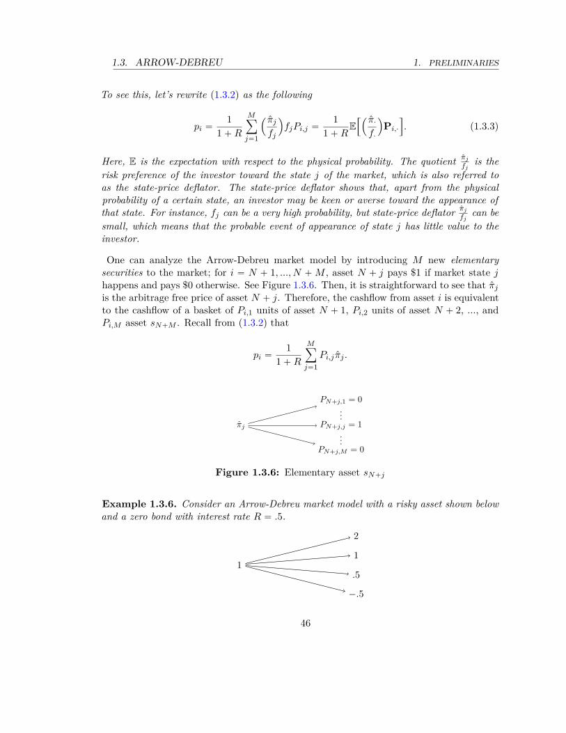
1.3. ARROW-DEBREU 1. PRELIMINARIES
To see this, let’s rewrite (1.3.2) as the following
pi “1
1 ` R
Mÿ
j“1
´ πj
fj
¯
fjPi,j “1
1 ` RE”´ π¨
f¨
¯
Pi,¨
ı
. (1.3.3)
Here, E is the expectation with respect to the physical probability. The quotient πj
fjis the
risk preference of the investor toward the state j of the market, which is also referred toas the state-price deflator. The state-price deflator shows that, apart from the physicalprobability of a certain state, an investor may be keen or averse toward the appearance ofthat state. For instance, fj can be a very high probability, but state-price deflator πj
fjcan be
small, which means that the probable event of appearance of state j has little value to theinvestor.
One can analyze the Arrow-Debreu market model by introducing M new elementarysecurities to the market; for i “ N ` 1, ..., N ` M , asset N ` j pays $1 if market state jhappens and pays $0 otherwise. See Figure 1.3.6. Then, it is straightforward to see that πj
is the arbitrage free price of asset N ` j. Therefore, the cashflow from asset i is equivalentto the cashflow of a basket of Pi,1 units of asset N ` 1, Pi,2 units of asset N ` 2, ..., andPi,M asset sN`M . Recall from (1.3.2) that
pi “1
1 ` R
Mÿ
j“1Pi,j πj .
πj
PN+j,1 = 0...
PN+j,j = 1...
PN+j,M = 0
Figure 1.3.6: Elementary asset sN`j
Example 1.3.6. Consider an Arrow-Debreu market model with a risky asset shown belowand a zero bond with interest rate R “ .5.
1
2
1
.5
−.5
46
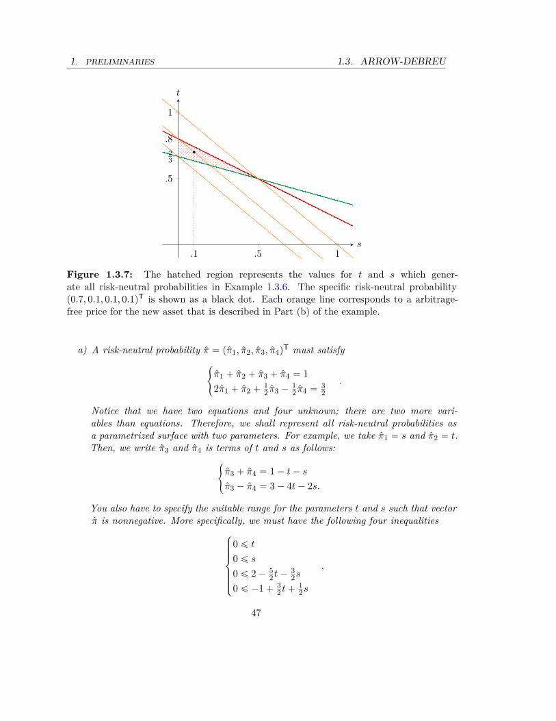
1. PRELIMINARIES 1.3. ARROW-DEBREU
.1 .5 1
.5
.8
1
23
s
t
Figure 1.3.7: The hatched region represents the values for t and s which gener-ate all risk-neutral probabilities in Example 1.3.6. The specific risk-neutral probabilityp0.7, 0.1, 0.1, 0.1qT is shown as a black dot. Each orange line corresponds to a arbitrage-free price for the new asset that is described in Part (b) of the example.
a) A risk-neutral probability π “ pπ1, π2, π3, π4qT must satisfy#
π1 ` π2 ` π3 ` π4 “ 12π1 ` π2 ` 1
2 π3 ´ 12 π4 “ 3
2.
Notice that we have two equations and four unknown; there are two more vari-ables than equations. Therefore, we shall represent all risk-neutral probabilities asa parametrized surface with two parameters. For example, we take π1 “ s and π2 “ t.Then, we write π3 and π4 is terms of t and s as follows:
#
π3 ` π4 “ 1 ´ t ´ s
π3 ´ π4 “ 3 ´ 4t ´ 2s.
You also have to specify the suitable range for the parameters t and s such that vectorπ is nonnegative. More specifically, we must have the following four inequalities
$
’
’
’
’
&
’
’
’
’
%
0 ď t
0 ď s
0 ď 2 ´ 52 t ´ 3
2s
0 ď ´1 ` 32 t ` 1
2s
,
47
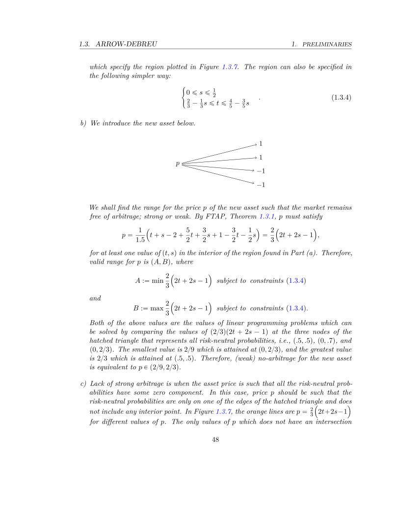
1.3. ARROW-DEBREU 1. PRELIMINARIES
which specify the region plotted in Figure 1.3.7. The region can also be specified inthe following simpler way:
#
0 ď s ď 12
23 ´ 1
3s ď t ď 45 ´ 3
5s. (1.3.4)
b) We introduce the new asset below.
p
1
1
−1
−1
We shall find the range for the price p of the new asset such that the market remainsfree of arbitrage; strong or weak. By FTAP, Theorem 1.3.1, p must satisfy
p “1
1.5
´
t ` s ´ 2 `52
t `32
s ` 1 ´32
t ´12
s¯
“23
´
2t ` 2s ´ 1¯
,
for at least one value of pt, sq in the interior of the region found in Part (a). Therefore,valid range for p is pA, Bq, where
A :“ min 23
´
2t ` 2s ´ 1¯
subject to constraints (1.3.4)
andB :“ max 2
3
´
2t ` 2s ´ 1¯
subject to constraints (1.3.4).
Both of the above values are the values of linear programming problems which canbe solved by comparing the values of p23qp2t ` 2s ´ 1q at the three nodes of thehatched triangle that represents all risk-neutral probabilities, i.e., p.5, .5q, p0, .7q, andp0, 23q. The smallest value is 29 which is attained at p0, 23q, and the greatest valueis 23 which is attained at p.5, .5q. Therefore, (weak) no-arbitrage for the new assetis equivalent to p P p29, 23q.
c) Lack of strong arbitrage is when the asset price is such that all the risk-neutral prob-abilities have some zero component. In this case, price p should be such that therisk-neutral probabilities are only on one of the edges of the hatched triangle and doesnot include any interior point. In Figure 1.3.7, the orange lines are p “ 2
3
´
2t`2s´1¯
for different values of p. The only values of p which does not have an intersection
48

1. PRELIMINARIES 1.3. ARROW-DEBREU
with the interior of the triangle are p “ 29 and p “ 23. Therefore, the lack ofstrong arbitrage implies that p P r29, 23s.
Exercise 1.3.4. Consider an Arrow-Debreu market model with N “ 3 and M “ 4 shownin Figure 1.3.8 and take the bond yield R “ 0, where v1 and v2 are two (distinct) realnumbers.
p1 = v1+v2
2
P1,1 = v1
P1,2 = v2
P1,3 = v1
P1,4 = v2
p2 = v1+v2
2
P2,1 = v1
P2,2 = v1
P2,3 = v2
P2,4 = v2
Figure 1.3.8: Exercise 1.3.4
a) Find all risk-neutral probabilities.
b) Recall the notion of independent random variables. Find a risk-neutral probabilitythat makes the random variables of the prices of two assets independent.
1.3.3 One-period binomial model
Let M “ 2 and N “ 2 with one risk-free zero bond and a risky asset with price S0 :“ p1,and future cash flow given byP1,1 “ S0u and P1,2 “ S0ℓ where S0 and ℓ ă u are all positivereal numbers. By Theorem 1.3.1, in a one-period binomial model, no-arbitrage condition
S0
S0u
S0ℓ
Figure 1.3.9: One-period binomial model
49

1.3. ARROW-DEBREU 1. PRELIMINARIES
is equivalent to ℓ ă 1 ` R ă u and π “ pπℓ, πuqT with πu “ 1`R´ℓpu´ℓqp1`Rq
and πℓ “ u´1´Rpu´ℓqp1`Rq
.The risk-neutral probability is then given by πu “ 1`R´ℓ
u´ℓ and πℓ “ u´1´Ru´ℓ .
Exercise 1.3.5. Show the above claims.
From FTAP, we know that ℓ ă 1`R ă u is equivalent to the no-arbitrage condition. But,it is often insightful to construct an arbitrage portfolio when ℓ ă 1 ` R ă u is violated.For example, consider the case when u ď 1 ` R. Then, consider a portfolio with a shortposition in one unit of the asset and a long position in S0 units of bonds. To constructthis portfolio, no cash is needed, and it is worth zero. However, the two possible futureoutcomes are either S0p1 ` Rq ´ S0u ě 0 or S0p1 ` Rq ´ S0ℓ ą 0, which matches withthe definition of (weak) arbitrage in Definition 1.3.1. If we assume the strict inequalityu ă 1 ` R, then the arbitrage is strong.Next, we consider the addition of a new asset into the market with payoff P1 and P2 in
states 1 and 2, respectively. Then, no-arbitrage condition implies that the price p of thisasset is must be given by
p “1
1 ` RpπuP1 ` πℓP2q .
In particular, if the new asset is an option with payoff function gpS1q, the no arbitrageprice V pS0q of the option is given by
V pS0q :“ 11 ` R
´
πugpS0uq ` πℓgpS0ℓq
¯
“1
1 ` RErgpS1qs. (1.3.5)
Here, E is the expectation under probability π, and S1 is a random variable of the priceof asset at time t “ 1 that takes the values S0ℓ and S0u. For instance, a call option withpayoff pS ´ Kq` with ℓS0 ď K ă uS0, shown in figure 1.3.10, has a “no-arbitrage price”:
CpKq “1 ` R ´ ℓ
pu ´ ℓqp1 ` RqpuS0 ´ Kq.
C(K)
S0u−K
0
Figure 1.3.10: Cashflow of a call option in a one-period binomial model
50

1. PRELIMINARIES 1.3. ARROW-DEBREU
We shall now see why any price other than puS0´Kq
p1`Rqπu for the call option causes arbitrage
in the binomial market with a zero bond, a risky asset and a call option on the risky asset.For this reason, we need to first introduce the notion of a replicating portfolio. Consider aportfolio with θ0 investment in a zero bond and θ1 units of risky asset. Then, this portfoliogenerates the cashflow shown in Figure 1.3.11. We want to choose pθ0, θ1q such that thepayoff of this portfolio matches the payoff of the call option, i.e.
#
θ0 ` θ1S0u “ S0u ´ K
θ0 ` θ1S0ℓ “ 0(1.3.6)
Therefore, we have to choose
θ0 “ ´lpS0u ´ Kq
u ´ ℓand θ1 “
S0u ´ K
S0pu ´ ℓq.
θ01+R + θ1S0
θ0 + θ1S0u = S0u−K
θ0 + θ1S0ℓ = 0
Figure 1.3.11: Replicating portfolio in a one-period binomial model
Then, one can see that the value of the replicating portfolio is equal to the price of thecall option, i.e.,
θ01 ` R
` θ1S0 “ ´lpS0u ´ Kq
p1 ` Rqpu ´ ℓq`
S0u ´ K
u ´ ℓ“
11 ` R
pS0 ´ Kqπu.
Now, we return to building an arbitrage in the case where the price of call option C isdifferent from puS0´Kq
p1`Rqπu. We only cover the case C ă
puS0´Kq
p1`Rqπu. Consider a portfolio that
consists of a long position in a call option and a short position in a replicating portfolioon the same call option. Shorting a replicating portfolio is equivalent to a ´θ0 positionin cash, and a ´θ1 position in the underlying asset. Then, the value of such a portfoliois equal to C ´
puS0´Kq
p1`Rqπu ă 0. This means that there is some extra cash in the pocket,
while the payoff of the call option can be used to clear off the shorted replicating portfolioin full. Here, the arbitrage is in the strong sense of Definition 1.3.2.A replicating portfolio can be built for any payoff gpS1q by solving the system of equations
51

1.3. ARROW-DEBREU 1. PRELIMINARIES
#
θ0 ` θ1S0u “ gpS0uq
θ0 ` θ1S0ℓ “ gpS0ℓq(1.3.7)
to obtainθ0 “
ugpS0ℓq ´ ℓgpS0uq
u ´ ℓand θ1 “
gpS0uq ´ gpS0ℓq
S0pu ´ ℓq.
The value of the replicating portfolio is given by
θ01 ` R
` θ1S0 “ugpS0ℓq ´ ℓgpS0uq
p1 ` Rqpu ´ ℓq`
gpS0uq ´ gpS0ℓq
u ´ ℓ“
11 ` R
pπugpS0uq ` πℓgpS0ℓqq,
which is equal to the expected value of the discounted payoff under risk-neutral probability.
Exercise 1.3.6. Consider a one-period binomial model with parameters ℓ, u and R andlet K P pS0ℓ, S0us. Find a replicating portfolio for a put option with strike K. Verify thatthe value of the replicating portfolio is equal to the no-arbitrage price of the put optionP pKq “ πℓpK ´ S0ℓq. Then, find an arbitrage portfolio when the price of the put optionwith strike K is less than P pKq.Exercise 1.3.7. Consider an Arrow-Debreu market model with M “ 2 that consists of arisk-free bond with interest rate R “ .01 and a forward contract11 on a nonstorable asset12
with forward price K and maturity of one period. Given that the payoff of the forwardcontract for the long position takes values P1,1 “ 4, and P1,2 “ ´2 respective to the stateof the market at maturity, is there any arbitrage?Now assume that the underlying asset is storable and has price p “ 10. Given that there isno arbitrage, find K, and binomial model parameters u and d for the underlying asset.Example 1.3.7. Consider the binomial model with S0 “ 4, R “ .05, u “ 1.45, and ℓ “ .85.We shall price and replicate the payoff g in Figure 1.3.12 . To find the replicating portfolio,we solve the system of equations (1.3.7)
#
θ0 ` 5.8θ1 “ gp5.8q “ .8θ0 ` 3.4θ1 “ gp3.4q “ .6
to obtain θ0 “ 1.96 and θ1 “ 1
12 . The price can be found in two ways: either by using thereplicating portfolio or by the risk-neutral probability. The former gives the price by thevalue of the replicating portfolio:
θ01 ` R
` θ1S0 “1.9
6p1.05q` p4q
112
“2
3.15.
11In the context of this exercise, the forward can be replaced by a futures contract.12E.g. electricity.
52
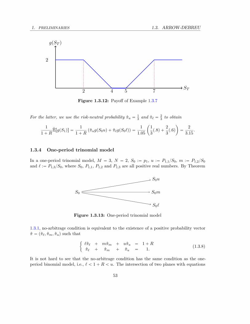
1. PRELIMINARIES 1.3. ARROW-DEBREU
2 74 5
2
ST
g(ST )
Figure 1.3.12: Payoff of Example 1.3.7
For the latter, we use the risk-neutral probability πu “ 13 and πℓ “ 2
3 to obtain
11 ` R
ErgpS1qs “1
1 ` RpπugpS0uq ` πℓgpS0ℓqq “
11.05
ˆ
13
p.8q `23
p.6q
˙
“2
3.15.
1.3.4 One-period trinomial model
In a one-period trinomial model, M “ 3, N “ 2, S0 :“ p1, u :“ P1,1S0, m :“ P1,2S0and ℓ :“ P1,3S0, where S0, P1,1, P1,2 and P1,3 are all positive real numbers. By Theorem
S0
S0u
S0m
S0ℓ
Figure 1.3.13: One-period trinomial model
1.3.1, no-arbitrage condition is equivalent to the existence of a positive probability vectorπ “ pπℓ, πm, πuq such that
"
ℓπℓ ` mπm ` uπu “ 1 ` Rπℓ ` πm ` πu “ 1.
(1.3.8)
It is not hard to see that the no-arbitrage condition has the same condition as the one-period binomial model, i.e., ℓ ă 1 ` R ă u. The intersection of two planes with equations
53

1.3. ARROW-DEBREU 1. PRELIMINARIES
(1.3.8) in R3 is a line parametrized by$
’
&
’
%
πℓ “u´p1`Rq
u´ℓ ´ m´ℓu´ℓ t
πm “ t
πu “ 1`R´ℓu´ℓ ´ u´m
u´ℓ t
The no-arbitrage condition is equivalent to the existence of a segment of this line in thepositive octane; i.e., there exists a t such that
$
’
&
’
%
πℓ “u´p1`Rq
u´ℓ ´ m´ℓu´ℓ t ą 0
πm “ t ą 0πu “ 1`R´ℓ
u´ℓ ´ u´mu´ℓ t ą 0
,
which is guaranteed if and only if 0 ă min!
1`R´ℓu´m , u´p1`Rq
m´ℓ
)
. Or equivalently, ℓ ă 1`R ă u.
Notice that the positive segment is given by 0 ă t ă min!
1`R´ℓu´m , u´p1`Rq
m´ℓ
)
.
u1+R
1
m1+R
1
ℓ1+R
1
πℓ
πm
πu
Figure 1.3.14: The positive segment of line given by (1.3.8) when ℓ ă 1 ` R ă u
Exercise 1.3.8. Derive the no-arbitrage condition for the multinomial model in Figure1.3.15. Here, u1 ă u2 ă ¨ ¨ ¨ ă uM are positive numbers.
54
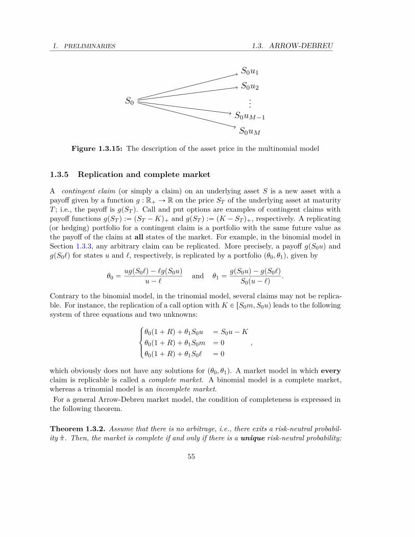
1. PRELIMINARIES 1.3. ARROW-DEBREU
S0
S0u1
S0u2
...S0uM−1
S0uM
Figure 1.3.15: The description of the asset price in the multinomial model
1.3.5 Replication and complete market
A contingent claim (or simply a claim) on an underlying asset S is a new asset with apayoff given by a function g : R` Ñ R on the price ST of the underlying asset at maturityT ; i.e., the payoff is gpST q. Call and put options are examples of contingent claims withpayoff functions gpST q :“ pST ´ Kq` and gpST q :“ pK ´ ST q`, respectively. A replicating(or hedging) portfolio for a contingent claim is a portfolio with the same future value asthe payoff of the claim at all states of the market. For example, in the binomial model inSection 1.3.3, any arbitrary claim can be replicated. More precisely, a payoff gpS0uq andgpS0ℓq for states u and ℓ, respectively, is replicated by a portfolio pθ0, θ1q, given by
θ0 “ugpS0ℓq ´ ℓgpS0uq
u ´ ℓand θ1 “
gpS0uq ´ gpS0ℓq
S0pu ´ ℓq.
Contrary to the binomial model, in the trinomial model, several claims may not be replica-ble. For instance, the replication of a call option with K P rS0m, S0uq leads to the followingsystem of three equations and two unknowns:
$
’
&
’
%
θ0p1 ` Rq ` θ1S0u “ S0u ´ K
θ0p1 ` Rq ` θ1S0m “ 0θ0p1 ` Rq ` θ1S0ℓ “ 0
,
which obviously does not have any solutions for pθ0, θ1q. A market model in which everyclaim is replicable is called a complete market. A binomial model is a complete market,whereas a trinomial model is an incomplete market.For a general Arrow-Debreu market model, the condition of completeness is expressed in
the following theorem.
Theorem 1.3.2. Assume that there is no arbitrage, i.e., there exits a risk-neutral probabil-ity π. Then, the market is complete if and only if there is a unique risk-neutral probability;
55

1.3. ARROW-DEBREU 1. PRELIMINARIES
i.e., if and only if the system of linear equation (1.3.1)
p “ Pπ
has a unique positive solution.
While in the binomial model there is only one risk-neutral probability and therefore themarket is complete, in the trinomial model there are infinitely many risk-neutral probabil-ities and therefore the market is incomplete.
1.3.6 superreplication and model risk
Replication (or hedging) is a normal practice for the issuer of an option to manage the riskof issuing that option. When the market is not complete, one cannot perfectly replicate allclaims and the issuer of a claim should take another approach: a nonperfect replication.In practice, the replication starts only after pricing the claim. The issuer first picks upa pricing model, i.e., a risk-neutral probability π˚ “ pπ˚
1 , ..., π˚M qT, to price the claim by
11`R E˚rgpST qs. Then, she tries to use the fund raised by selling the option to find anonperfect replication strategy. Genuinely, the higher the price of the claim, the less theissuer is exposed to the risk. Therefore, the chosen risk-neutral probability π˚ to pricethe claims represents some level of exposure to the risk. In this section, we would like toprovide a method to measure this risk, namely model risk.The choice of a replication strategy usually depends on many variables, including the
risk preference of the issuer, which are outside the context of this section. However, forthe purpose of model risk, we introduce one specific choice of a nonperfect replicationstrategy, namely superreplication. A superreplication strategy prepares the issuer for theworst-case scenario. The superreplication price of an option is defined as the cheapest priceof a portfolio that generates a payoff greater than or equal to the payoff the option for allstates of the market. In the Arrow-Debreu market model for asset shown in Figure 1.3.15,we want to make a portfolio pθ0, θ1q such that
θ0 ` θ1S0uj ě gpS0ujq for all j “ 1, ..., M.
Then, among all such portfolios we want to choose the one that has the least cost, i.e.,min θ0
1`R ` θ1S0. For instance, in the trinomial model, the superreplication price of anoption with payoff gpS1q is defined by
min θ01 ` R
` θ1S0 (1.3.9)
56
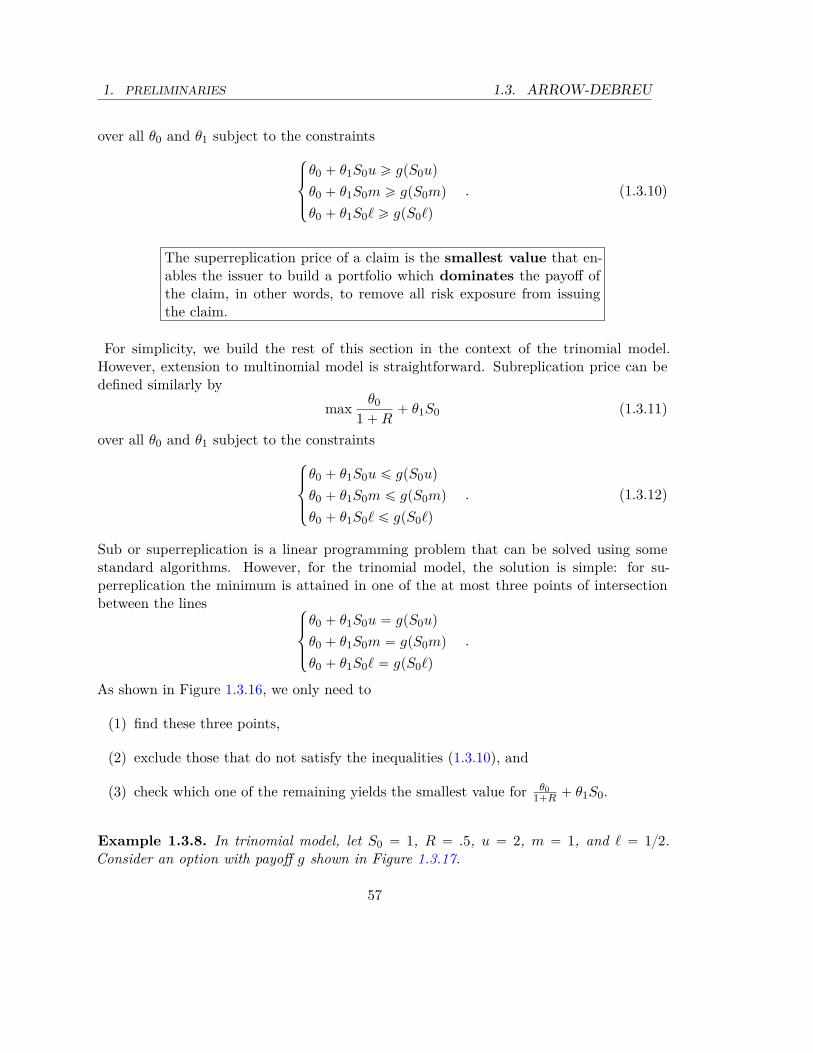
1. PRELIMINARIES 1.3. ARROW-DEBREU
over all θ0 and θ1 subject to the constraints$
’
&
’
%
θ0 ` θ1S0u ě gpS0uq
θ0 ` θ1S0m ě gpS0mq
θ0 ` θ1S0ℓ ě gpS0ℓq
. (1.3.10)
The superreplication price of a claim is the smallest value that en-ables the issuer to build a portfolio which dominates the payoff ofthe claim, in other words, to remove all risk exposure from issuingthe claim.
For simplicity, we build the rest of this section in the context of the trinomial model.However, extension to multinomial model is straightforward. Subreplication price can bedefined similarly by
max θ01 ` R
` θ1S0 (1.3.11)
over all θ0 and θ1 subject to the constraints$
’
&
’
%
θ0 ` θ1S0u ď gpS0uq
θ0 ` θ1S0m ď gpS0mq
θ0 ` θ1S0ℓ ď gpS0ℓq
. (1.3.12)
Sub or superreplication is a linear programming problem that can be solved using somestandard algorithms. However, for the trinomial model, the solution is simple: for su-perreplication the minimum is attained in one of the at most three points of intersectionbetween the lines
$
’
&
’
%
θ0 ` θ1S0u “ gpS0uq
θ0 ` θ1S0m “ gpS0mq
θ0 ` θ1S0ℓ “ gpS0ℓq
.
As shown in Figure 1.3.16, we only need to
(1) find these three points,
(2) exclude those that do not satisfy the inequalities (1.3.10), and
(3) check which one of the remaining yields the smallest value for θ01`R ` θ1S0.
Example 1.3.8. In trinomial model, let S0 “ 1, R “ .5, u “ 2, m “ 1, and ℓ “ 12.Consider an option with payoff g shown in Figure 1.3.17.
57

1.3. ARROW-DEBREU 1. PRELIMINARIES
θ0
θ1
Figure 1.3.16: The linear programing problem for superhedging. The hatched region isdetermined by constraints (1.3.10). The dashed lines are the contours of the linear function
θ01`R ` θ1S0 in (1.3.9). The point marked by ˛ is where the minimum is attained.
1
1
2ST
g(ST )
Figure 1.3.17: Payoff of Example 1.3.8
a) Notice that payoff gp2q “ 0 and gp1q “ gp12q “ 1. We shall find the superreplicationprice for this option.
min 2θ03
` θ1
58
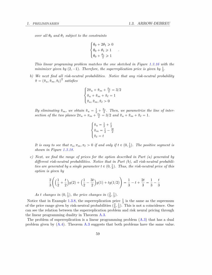
1. PRELIMINARIES 1.3. ARROW-DEBREU
over all θ0 and θ1 subject to the constraints$
’
&
’
%
θ0 ` 2θ1 ě 0θ0 ` θ1 ě 1θ0 ` θ1
2 ě 1.
This linear programing problem matches the one sketched in Figure 1.3.16 with theminimizer given by p2, ´1q. Therefore, the superreplication price is given by 1
3 .
b) We next find all risk-neutral probabilities. Notice that any risk-neutral probabilityπ “ pπu, πm, πℓq
T satisfies$
’
&
’
%
2πu ` πm ` πℓ2 “ 32
πu ` πm ` πℓ “ 1πu, πm, πℓ ą 0
By eliminating πm, we obtain πu “ 12 ` πℓ
2 . Then, we parametrize the line of inter-section of the two planes 2πu ` πm ` πℓ
2 “ 32 and πu ` πm ` πℓ “ 1.$
’
&
’
%
πu “ 12 ` t
2πm “ 1
2 ´ 3t2
πℓ “ t
It is easy to see that πu, πm, πℓ ą 0 if and only if t P p0, 13q. The positive segment is
shown in Figure 1.3.18.
c) Next, we find the range of prices for the option described in Part (a) generated bydifferent risk-neutral probabilities. Notice that in Part (b), all risk-neutral probabili-ties are generated by a single parameter t P p0, 1
3q. Thus, the risk-neutral price of thisoption is given by
23
˜
´12
`t
2
¯
gp2q `
´12
´3t
2
¯
gp1q ` tgp12q
¸
“13
´ t `2t
3“
13
´t
3
As t changes in p0, 13q, the price changes in p2
9 , 13q.
Notice that in Example 1.3.8, the superreplication price 13 is the same as the supremum
of the price range given by risk-neutral probabilities p29 , 1
3q. This is not a coincidence. Onecan see the relation between the superreplication problem and risk neural pricing throughthe linear programming duality in Theorem A.3.The problem of superreplication is a linear programming problem (A.3) that has a dual
problem given by (A.4). Theorem A.3 suggests that both problems have the same value.
59

1.3. ARROW-DEBREU 1. PRELIMINARIES
.75
1
1.5
1
3
1
πℓ
πm
πu
Figure 1.3.18: The positive segment of the intersection of two lines given by πuu`πmm`
πℓℓ “ 1 ` R and πu ` πm ` πℓ “ 1. The mark on the segment represents a chosen pricingmodel π˚.
In the context of superreplication for the trinomial model, the dual problem is given by
max πugpS0uq ` πmgpS0mq ` πℓgpS0mq
over all πℓ, πm, and πu subject to the constraints$
’
&
’
%
πuS0u ` πmS0m ` πℓS0m “ S0
πu ` πm ` πℓ “ 11`R
πu, πm, πℓ ě 0
By change of variable π “ p1 ` Rqπ, the dual problem turns into
Ppgq :“ 11 ` R
max πugpS0uq ` πmgpS0mq ` πℓgpS0mq, subject to$
’
&
’
%
πuu ` πmm ` πℓℓ “ 1 ` R
πu ` πm ` πℓ “ 1πu, πm, πℓ ě 0
.(1.3.13)
Given no-arbitrage condition, the line of intersection of two planes πuu`πmm`πℓℓ “ 1`Rand πu ` πm ` πℓ “ 1 has a segment in the positive octane, shown in Figure 1.3.14. Then,the value of Ppgq in (1.3.13) is attained at one of endpoints of this segment. This segmentrepresents the set of all risk-neutral probabilities. According to Theorem 1.3.1, the lack ofweak arbitrage implies that this segment is inside the first octane with to endpoints on twodifferent coordinate planes, and the lack of strong arbitrage only implies that the endpoints
60

1. PRELIMINARIES 1.3. ARROW-DEBREU
of the segment are on the coordinate planes, possibly the same coordinate plane.Let’s recall what we presented at the beginning of this section: the issuer of the option
chooses a risk-neutral probability π˚ inside the positive segment to price the option. Theendpoints of this segment, one of which maximizes and the other minimizes the value
11`R max πugpS0uq ` πmgpS0mq ` πℓgpS0mq, provide the super and subreplication price ofthe option with payoff g, respectively. While the issuer has priced the claim by
11 ` R
E˚rgpS1qs,
to completely cover the risk, he needs P in (1.3.13). Therefore, he is short as much as
Θpπ˚q :“ Ppgq ´1
1 ` RE˚rgpS1qs
in order to cover the risk of issuing the claim. The value Θpπ˚q is called superreplicationmodel risk measure.
Example 1.3.9. In Example 1.3.8, if the pricing probability π˚ “ p712, 14, 16qT ischosen, then the superreplication model risk is measured by
Ppgq ´1
1 ` RE˚rgpS1qs “
13
´23
˜
712
gp2q `14
gp1q `16
gp12q
¸
“13
´518
“118
.
Exercise 1.3.9. In the trinomial model, let S0 “ 1, R “ 0, u “ 2, m “ 1, and ℓ “ 12.
a) Find all the risk-neutral probabilities and the range of prices generated by them for acall option with strike K “ 1.
b) Find the superreplication price and sub-replication price for this call option and com-pare them to the lowest and highest prices in Part (a).
Example 1.3.10. In Example 1.3.8, if we modify the yield by setting R “ 1, then therewill be an arbitrage. This can be seen through the absence of risk-neutral probabilities. Onthe other hand, the superreplication problem is still feasible, i.e., problem (1.3.11) withconstraint (1.3.10) still has a finite value. But this value is zero. This is because weminimize θ0
2 ` θ1 subject to θ0 ` 2θ1 ě 0, θ0 ` θ1 ě 1 and θ0 ` θ12 ě 1, which obviously takes
minimum value zero.On the other hand, if we set R ą 1, then the superreplication problem is not feasible
anymore and the minimum is ´8.
Example 1.3.11. Consider the trinomial model with S0 “ 4, R “ .05, u “ 1.45, m “
1.25 and ℓ “ .85. To price payoff g in Figure 1.3.12, the risk-neutral probability π “
pπu, πm, πℓqT “ p518, 112, 2336qT has been chosen. In order to find the model risk, we
61
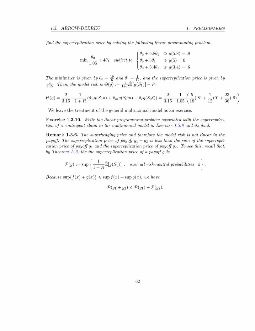
1.3. ARROW-DEBREU 1. PRELIMINARIES
find the superreplication price by solving the following linear programming problem.
min θ01.05
` 4θ1 subject to
$
’
&
’
%
θ0 ` 5.8θ1 ě gp5.8q “ .8θ0 ` 5θ1 ě gp5q “ 0θ0 ` 3.4θ1 ě gp3.4q “ .6
The minimizer is given by θ0 “ 196 and θ1 “ 1
12 , and the superreplication price is given by2
3.15 . Then, the model risk is Θpgq :“ 11`R ErgpS1qs ´ P.
Θpgq “2
3.15´
11 ` R
pπugpS0uq ` πmgpS0mq ` πℓgpS0ℓqq “2
3.15´
11.05
ˆ
518
p.8q `112
p0q `2336
p.6q
˙
We leave the treatment of the general multinomial model as an exercise.
Exercise 1.3.10. Write the linear programming problem associated with the superreplica-tion of a contingent claim in the multinomial model in Exercise 1.3.8 and its dual.
Remark 1.3.6. The superhedging price and therefore the model risk is not linear in thepayoff. The superreplication price of payoff g1 ` g2 is less than the sum of the superrepli-cation price of payoff g1 and the superreplication price of payoff g2. To see this, recall that,by Theorem A.3, the the superreplication price of a payoff g is
Ppgq :“ sup"
11 ` R
ErgpS1qs : over all risk-neutral probabilities π
*
.
Because suptfpxq ` gpxqu ď sup fpxq ` sup gpxq, we have
Ppg1 ` g2q ď Ppg1q ` Ppg2q.
62
2. DISCRETE-TIME MARKETS
2
Modeling financial assets indiscrete-time markets
Section 1.3 deals with a single-period market in which there are only two trading dates,one at the beginning of the period and one at maturity. In this part, we extend the resultsof Section 1.3 to a multiperiod market with a focus on the binomial model. This is alsoimportant in our later study of continuous-time markets, which can be seen as the limit ofdiscrete-time markets.
2.1 Arbitrage and trading in discrete-time markets
Consider a discrete-time market with time horizon T in which trading occurs only at timet “ 0, ..., T , and there are d assets. We shall denote the price of asset i at time t “ 0, ..., T
by Spiqt , for i “ 0, ..., d.
Canonical Space
The price of each risky asset in a multiperiod model is a stochastic process; this means foreach t “ 1, ..., T , the price at time t, denoted by St is a random variable. For this reason,we need to start off with a measure space pΩ, Fq or a probability space pΩ, F ,Pq.One useful choice of measure space pΩ, Fq is the canonical space; we take Ω :“ pRd`1
` qT 1
equipped with the Borel σ-field BppRd`1` qT q.
The motivation behind this choice is as follows. Each ω P Ω is made of T -tuples of theform pω1, ...ωT qT such that each ωt “ pω
piqt : i “ 0, ..., dq is a column d-vector, and ω
piqt is
interpreted as the value of the price of asset i at time t. The random variable Spiqt which
1We prefer to write pRd`1` qT and not Rpd`1qT
` .
63
2.1. TRADING AND ARBITRAGE 2. DISCRETE-TIME MARKETS
represents the price of asset i at time t is then defined by the canonical mapping
Spiqt : ω “
»
—
–
ω01 ¨ ¨ ¨ ω0
T... . . . ...
ωd1 ¨ ¨ ¨ ωd
T
fi
ffi
fl
ÞÑ ωpiqt .
We assume that the price of an asset only takes positive values ωpiqt P R`. If it takes
negative values, then we can extend the sample space to Ω :“ pRd`1qT , and all the resultsof this section hold immediately. If asset 0 is a risk-free asset, then we can remove itscontribution in the sample space and write Ω :“ pRd
`qT .The choice of canonical space allows us to cover all types of models for asset price, i.e.,
with discrete or nondiscrete distribution.
Portfolio
A self-financing portfolio, or simply a portfolio, is represented by the vector θt “ pθp0qt , ..., θ
pdqt qT
withdÿ
i“0θ
piqt “ 1, for t “ 0, ..., T ´ 1.
Here, θpiqt is the portion of value of the portfolio invested in asset i at time t; i.e., θ
piqt “
∆piqt S
piqt
Wt, where ∆piq
t is the number of shares of asset i in the portfolio, Spiqt is the current
price of asset i, and Wt is the total value of the portfolio all of them at time t. Moreprecisely,
Wt “
dÿ
i“0∆piq
t Spiqt .
θpiqt can be positive, negative, or zero, representing long, short, or no-investment positions
in asset i, respectively. Given initial wealth W0, the initial portfolio investment is shownin the first row in Table 2.1.We rigorously define the portfolio below.
Definition 2.1.1. A self-financing portfolio strategy is given by a sequence of vector func-tions θt “ pθ
p0qt , ..., θ
pdqt qT such that θ0 P Rd is a real vector and for t “ 1, ..., T ´ 1,
θt “ pθp0qt , ..., θ
pdqt qT : Ω Ñ Rd is a function that maps
St :“
»
—
–
S01 ¨ ¨ ¨ S0
t... . . . ...
Sd1 ¨ ¨ ¨ Sd
t
fi
ffi
fl
(2.1.1)
into a vector in Rd.
64
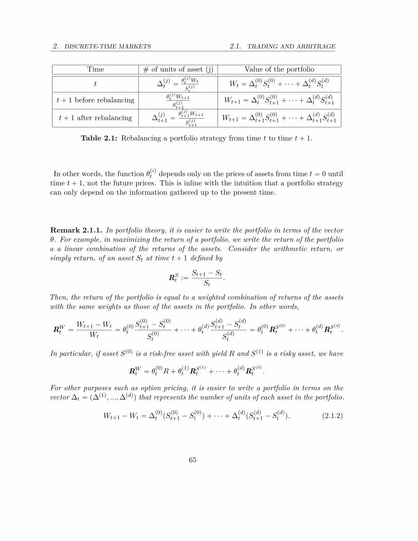
2. DISCRETE-TIME MARKETS 2.1. TRADING AND ARBITRAGE
Time # of units of asset (j) Value of the portfolio
t ∆pjqt “
θpjqt Wt
Spjqt
Wt “ ∆p0qt S
p0qt ` ¨ ¨ ¨ ` ∆pdq
t Spdqt
t ` 1 before rebalancing θpjqt Wt`1
Spjqt`1
Wt`1 “ ∆p0qt S
p0qt`1 ` ¨ ¨ ¨ ` ∆pdq
t Spdqt`1
t ` 1 after rebalancing ∆pjqt`1 “
θpjqt`1Wt`1
Spjqt`1
Wt`1 “ ∆p0qt`1S
p0qt`1 ` ¨ ¨ ¨ ` ∆pdq
t`1Spdqt`1
Table 2.1: Rebalancing a portfolio strategy from time t to time t ` 1.
In other words, the function θpiqt depends only on the prices of assets from time t “ 0 until
time t ` 1, not the future prices. This is inline with the intuition that a portfolio strategycan only depend on the information gathered up to the present time.
Remark 2.1.1. In portfolio theory, it is easier to write the portfolio in terms of the vectorθ. For example, in maximizing the return of a portfolio, we write the return of the portfolioa a linear combination of the returns of the assets. Consider the arithmetic return, orsimply return, of an asset St at time t ` 1 defined by
RSt :“ St`1 ´ St
St.
Then, the return of the portfolio is equal to a weighted combination of returns of the assetswith the same weights as those of the assets in the portfolio. In other words,
RWt “
Wt`1 ´ Wt
Wt“ θ
p0qt
Sp0qt`1 ´ S
p0qt
Sp0qt
` ¨ ¨ ¨ ` θpdqt
Spdqt`1 ´ S
pdqt
Spdqt
“ θp0qt RSp0q
t ` ¨ ¨ ¨ ` θpdqt RSpdq
t .
In particular, if asset Sp0q is a risk-free asset with yield R and Sp1q is a risky asset, we have
RWt “ θ
p0qt R ` θ
p1qt RSp1q
t ` ¨ ¨ ¨ ` θpdqt RSpdq
t .
For other purposes such as option pricing, it is easier to write a portfolio in terms on thevector ∆t “ p∆p1q, ..., ∆pdqq that represents the number of units of each asset in the portfolio.
Wt`1 ´ Wt “ ∆p0qt pS
p0qt`1 ´ S
p0qt q ` ¨ ¨ ¨ ` ∆pdq
t pSpdqt`1 ´ S
pdqt q. (2.1.2)
65
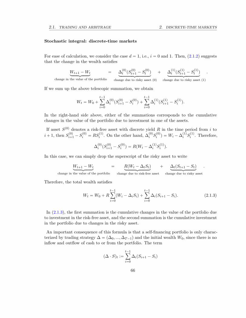
2.1. TRADING AND ARBITRAGE 2. DISCRETE-TIME MARKETS
Stochastic integral: discrete-time markets
For ease of calculation, we consider the case d “ 1, i.e., i “ 0 and 1. Then, (2.1.2) suggeststhat the change in the wealth satisfies
Wt`1 ´ Wtlooooomooooon
change in the value of the portfolio
“ ∆p0qt pS
p0qt`1 ´ S
p0qt q
loooooooooomoooooooooon
change due to risky asset (0)
` ∆p1qt pS
p1qt`1 ´ S
p1qt q
loooooooooomoooooooooon
change due to risky asset (1)
.
If we sum up the above telescopic summation, we obtain
Wt “ W0 `
t´1ÿ
i“0∆p0q
i pSp0qi`1 ´ S
p0qi q `
t´1ÿ
i“0∆p1q
i pSp1qi`1 ´ S
p1qi q.
In the right-hand side above, either of the summations corresponds to the cumulativechanges in the value of the portfolio due to investment in one of the assets.
If asset Sp0q denotes a risk-free asset with discrete yield R in the time period from i toi ` 1, then S
p0qi`1 ´ S
p0qi “ RS
p1qi . On the other hand, ∆p0q
i Sp0qi q “ Wi ´ ∆p1q
i Sp1qi . Therefore,
∆p0qi pS
p0qi`1 ´ S
p0qi q “ RpWi ´ ∆p1q
i Sp1qi q.
In this case, we can simply drop the superscript of the risky asset to write
Wt`1 ´ Wtlooooomooooon
change in the value of the portfolio
“ RpWt ´ ∆tStqlooooooomooooooon
change due to risk-free asset
` ∆tpSt`1 ´ Stqlooooooomooooooon
change due to risky asset
.
Therefore, the total wealth satisfies
Wt “ W0 ` Rt´1ÿ
i“0pWi ´ ∆iSiq `
t´1ÿ
i“0∆ipSi`1 ´ Siq. (2.1.3)
In (2.1.3), the first summation is the cumulative changes in the value of the portfolio dueto investment in the risk-free asset, and the second summation is the cumulative investmentin the portfolio due to changes in the risky asset.
An important consequence of this formula is that a self-financing portfolio is only charac-terized by trading strategy ∆ “ p∆0, ..., ∆T ´1q and the initial wealth W0, since there is noinflow and outflow of cash to or from the portfolio. The term
p∆ ¨ Sqt :“t´1ÿ
i“0∆ipSi`1 ´ Siq
66

2. DISCRETE-TIME MARKETS 2.1. TRADING AND ARBITRAGE
is called a discrete stochastic integral2.
Exercise 2.1.1. Let Wt :“ p1 ` Rq´tWt and St :“ p1 ` Rq´tSt be, respectively, discountedwealth process and discounted asset price. Then, show that
Wt “ W0 `
t´1ÿ
i“0∆ipSi`1 ´ Siq, W0 “ W0.
To understand the meaning of stochastic integral p∆ ¨ Sqt, we provide the following exam-ple.
Example 2.1.1. Recall from Example B.13 that a random walk W is the wealth of a playerin a game of chance in which he wins or loses $1 in each round based on the outcome offlipping a coin.Consider a modification of the game such that the player can bet a different amount of
money in each round of the game. For example, he can bet $3 in the first round and $5in the second round. If he loses the first round and wins the second, then his total wealthafter two rounds is $2. On the other hand, if he wins the first round and loses the secondround, he is short $2.If we denote the bet of the player in round i by ∆i´1, then the total wealth W∆ from the
betting strategy ∆ “ p∆0, ∆1, ...q in t rounds is given by
W∆t “ W∆
0 `
t´1ÿ
i“0∆iξi`1
where tξiui is a sequence of i.i.d. random variables with values `1 and ´1. Since ξi “
Wi`1 ´ Wi, we have
W∆t “
t´1ÿ
i“0∆ipWi`1 ´ Wiq “ p∆ ¨ Sqt.
In particular, if ∆i ” 1, W∆ “ W is merely a random walk.
Example 2.1.2 (Saint Petersburg paradox and doubling strategy). In Example 2.1.1, Weset the following strategy: ∆0 “ 1 and ∆i “ 2i, for i ą 0, if the player has lost all the pastrounds from 1 to i ´ 1. Otherwise, if the first winning occurs at round i, we set ∆j “ 0 forj ě i. For example, if the player’s outcome in the first five rounds are given by "loss, loss,loss, loss, win", then his bets are given by "1, 2, 4, 8, 16, 0 , ...", respectively. Then, thewealth of the player after five rounds is given by
W5 “ 1p´1q ` 2p´1q ` 4p´1q ` 8p´1q ` 16p1q “ 1.
2According to Philip Protter, this notation was devised by the prominent French probabilist Paul-AndréMeyer to simplify the task of typing with old-fashioned typewriters.
67
2.1. TRADING AND ARBITRAGE 2. DISCRETE-TIME MARKETS
However, his wealth before the fifth round is always negative.
W1 “ ´1, W2 “ ´3, W3 “ ´7, W4 “ ´15,
Exercise 2.1.2. a) Show that in Example 2.1.2 if the player has the opportunity toborrow with no limitation and continue the game until the first win, he will alwaysend up with terminal wealth equal to $1.
b) Assume that the player has a credit line, denoted by C. He stops playing if either hereaches his credit limit or he wins for the first time. Find the possible values for theterminal wealth of the player.
c) Find the expected value of the terminal wealth of the player, given that the probabilityof winning is p P p0, 1q.
Arbitrage strategy
In this section, we present the definition of an arbitrage opportunity and a FTAP3 formultistep discrete-time markets. In order to define arbitrage, we first need to determinethe set of all relevant events, by eliminating the impossible events, as part of modeling afinancial market. Relevant events are those that basically represent our beliefs about themarket behavior.
Definition 2.1.2. We call a collection of events N Ď BppRd`qT q a polar collection if it
satisfies
a) H P N .
b) If B P N and A Ď B, then A P N .
c) If tAnu8n“1 Ď N , then
Ť8n“1 An P N .
The members of a polar collection are called polar sets.
Example 2.1.3 (polar set). In the binomial model in Section 1.3.3, Ω “ R` is the canon-ical space, and the polar collection N is given by all subsets of Ω that do not contain anyof the points S0u or S0ℓ. Similarly, in the trinomial model in Section 1.3.4, Ω “ R` isthe canonical space and the polar collection N is the collection of all events A that do notcontain any of the points S0u, S0m, or S0ℓ.
The arbitrage in the context of polar set N is defined below.
Definition 2.1.3. A (weak) arbitrage opportunity is a portfolio ∆ such that3A fundamental theorem of asset pricing
68
2. DISCRETE-TIME MARKETS 2.1. TRADING AND ARBITRAGE
a) W0 “ 0,
b) tWT ă 0u P N , and
c) tWT ą 0u R N .
A strong arbitrage opportunity is a portfolio ∆ such that
a) W0 ă 0, and
b) tWT ě 0u R N .
For the distinction between the two notions of arbitrage see Remark 1.3.1.In the above discussion, we did not use any probability concept. However, to extend
FTAP to discrete-time multiperiod market models, we need the probabilistic notion ofmartingale, which is introduced in Section B.3. Risk-neutral probability can be defined interms of the martingale property for the discounted asset price: St :“ p1 ` Rq´tSt.
Definition 2.1.4. We call a probability P a risk-neutral probability if the discounted assetprice is a martingale with respect to P; i.e.,
ErSt`1 | St, St´1, ..., S1s “ St. (2.1.4)
Here E is the expectation with respect to P.
We also recall the notion of σ-field Ft generated by St, St´1, ..., S1 to write
ErSt`1 | Fts “ St.
For a single-period binomial model, the martingale property with respect to risk-neutralprobability is expressed and verified in Section 1.3.3; see (1.3.5).
Exercise 2.1.3. Show that if the discounted price St “ Stp1`Rqt is a martingale with respect
to probability P, then the stochastic integral p∆ ¨ Sqt and the discounted wealth process Wt
are martingales with respect to P.
The following result extends Theorem 1.3.1 into multiple periods. In order to have afundamental theorem of asset pricing in a general form, we need to impose the followingassumption.
Assumption 2.1.1 (Dominating probability). There exists a probability P such that A P Nif and only if PpAq “ 0.
The probability P can be regarded as the physical probability in the market. Therefore,one can equivalently define the collection of all polar sets as the set of all events that havezero probability under P. However, as seen in Theorem 2.1.1, the only relevant information
69
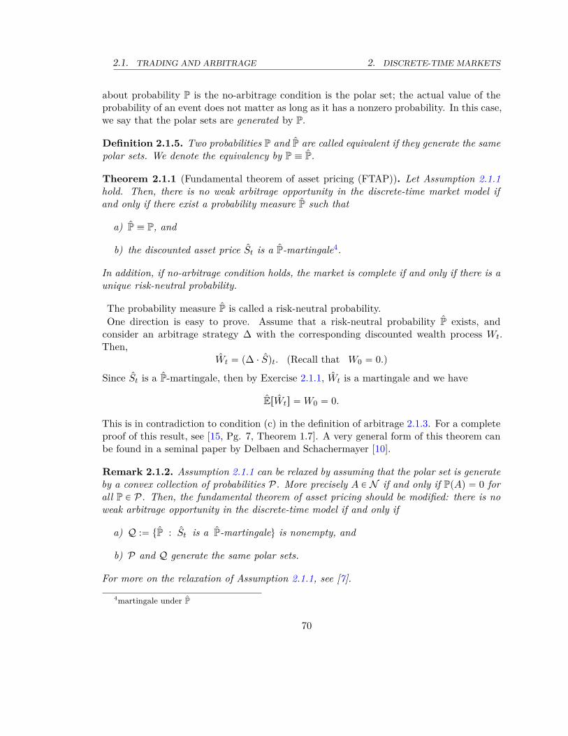
2.1. TRADING AND ARBITRAGE 2. DISCRETE-TIME MARKETS
about probability P is the no-arbitrage condition is the polar set; the actual value of theprobability of an event does not matter as long as it has a nonzero probability. In this case,we say that the polar sets are generated by P.
Definition 2.1.5. Two probabilities P and P are called equivalent if they generate the samepolar sets. We denote the equivalency by P ” P.
Theorem 2.1.1 (Fundamental theorem of asset pricing (FTAP)). Let Assumption 2.1.1hold. Then, there is no weak arbitrage opportunity in the discrete-time market model ifand only if there exist a probability measure P such that
a) P ” P, and
b) the discounted asset price St is a P-martingale4.
In addition, if no-arbitrage condition holds, the market is complete if and only if there is aunique risk-neutral probability.
The probability measure P is called a risk-neutral probability.One direction is easy to prove. Assume that a risk-neutral probability P exists, and
consider an arbitrage strategy ∆ with the corresponding discounted wealth process Wt.Then,
Wt “ p∆ ¨ Sqt. pRecall that W0 “ 0.q
Since St is a P-martingale, then by Exercise 2.1.1, Wt is a martingale and we have
ErWts “ W0 “ 0.
This is in contradiction to condition (c) in the definition of arbitrage 2.1.3. For a completeproof of this result, see [15, Pg. 7, Theorem 1.7]. A very general form of this theorem canbe found in a seminal paper by Delbaen and Schachermayer [10].
Remark 2.1.2. Assumption 2.1.1 can be relaxed by assuming that the polar set is generateby a convex collection of probabilities P. More precisely A P N if and only if PpAq “ 0 forall P P P. Then, the fundamental theorem of asset pricing should be modified: there is noweak arbitrage opportunity in the discrete-time model if and only if
a) Q :“ tP : St is a P-martingaleu is nonempty, and
b) P and Q generate the same polar sets.
For more on the relaxation of Assumption 2.1.1, see [7].
4martingale under P
70

2. DISCRETE-TIME MARKETS 2.2. BINOMIAL MODEL
A market model with no arbitrage is called a complete market model if any contingentclaim is replicable. In other words, for a contingent claim with payoff g : pRd`1
` qT Ñ Rwhich maps the history of an underlying asset price, S0, S1, ..., ST into gpS0, S1, ..., ST q,there exists a portfolio ∆0, ..., ∆T ´1 such that
p∆ ¨ SqT “ gpS0, S1, ..., ST q.
As an extension to Theorem 2.1.1, we have the following condition for the completeness ofa market.
Corollary 2.1.1. Let Assumption 2.1.1 and no-weak-arbitrage condition hold. Then, Themarket is complete if and only if there is a unique risk-neutral probability measure.
2.2 Binomial model
Let H1, H2, ... be an i.i.d.5 sequence of random variables with values u and ℓ6. Let thematurity be T , and let the time take values 0, 1, ..., T . At time 0, the price of the asset isS0. At time t “ 1, ..., T , the price of the asset satisfies St “ St´1Ht. The binomial modelis shown in Figure 2.2.1.We label the nodes of the binomial tree by the time and the state of the asset price. For
example, at time t when the asset price is equal to St,j`1 :“ S0ujlt´j , the node is labeledpt, j ` 1q. The only node at time 0 is labeled 0 for simplicity. See Figure 2.2.2.
2.2.1 No-arbitrage condition
The no-arbitrage condition for the multiperiod binomial model is the same as for the single-period. There is no arbitrage in the multiperiod binomial model if and only if there is noarbitrage for the single-period model with the same parameters.
Proposition 2.2.1. There is no arbitrage in multiperiod binomial model if and only ifℓ ă 1 ` R ă u. In this case, the multiperiod binomial market is complete, and the risk-neutral probability is given by assigning the following distribution to each Hi.
PpHi “ uq “1 ` R ´ ℓ
u ´ ℓand PpHi “ ℓq “
u ´ 1 ´ R
u ´ ℓ.
Proof. By Theorem 2.1.1 (FTAP), no-arbitrage condition is equivalent to the existenceof a risk-neutral probability. We first show that given ℓ ă 1 ` R ă u the probability Pdefined in the theorem is a risk-neutral probability. In other words, we shall show that
5Independent identically distributed6The probabilities of these values are irrelevant at this moment.
71

2.2. BINOMIAL 2. DISCRETE-TIME MARKETS
S0
S0u
S0ℓ
S0u2
S0uℓ
S0ℓ2
S0u3
S0u2ℓ
S0uℓ2
S0ℓ3
S0uT
S0uT−1ℓ
S0uT−2ℓ2
...
S0u2ℓT−2
S0uℓT−1
S0ℓT
Figure 2.2.1: Asset price in the binomial model
(0)
(1, 2)
(1, 1)
(2, 3)
(2, 2)
(2, 1)
(3, 4)
(3, 3)
(3, 2)
(3, 1)
Figure 2.2.2: Label of the nodes in a three-period binomial model
the discounted asset price is a martingale. Notice that since St`1 “ Ht`1St, we have
72

2. DISCRETE-TIME MARKETS 2.2. BINOMIAL
St`1 “Ht`11`R St. Therefore,
ErSt`1 | St, St´1, ..., S1s “1
1 ` RErStHt`1 | St, St´1, ..., S1s.
Since St is known given the condition tSt, St´1, ..., S1u, we can write
ErStHt`1 | St, St´1, ..., S1s “ StErHt`1 | St, St´1, ..., S1s.
On the other hand, since H1, H2, ... is a sequence of independent random variables, Ht`1is independent of the condition tSt, St´1, ..., S1u, and we have
ErHt`1 | St, St´1, ..., S1s “ ErHt`1 “ πuu ` πℓℓ “ 1 ` R.
Thus,ErSt`1 | St, St´1, ..., S1s “ St.
For the other direction, assume by contraposition that either u ď 1 ` R or ℓ ě 1 ` R.Then, Section 1.3.3 shows that there is an arbitrage in the first period. Then, one canliquidate the position to cash after the first period to carry over the arbitrage until timeT .
The above proof is also repeated in Example B.38.As shown in Figure 2.2.1, the random variable Sn takes values S0un´klk for k “ 0, ..., n.
Under the risk-neutral probability,
PpSn “ S0un´klkq “
ˆ
n
k
˙
pπuqn´k
pπℓqk .
To see this, notice that in the binomial tree in Figure 2.2.1, there are`
nk
˘
paths from thenode S0 to node S0un´klk, and the probability of each path is pπuq
n´kpπℓq
k7. We say thatat time t state i of the market occurs if St “ S0ut´ili for i “ 0, ..., t. For simplicity, wedenote S0ut´ili by Stpiq.
2.2.2 Basic properties of binomial tree
Binomial tree described above has some properties which are somehow features of manymodels in financial mathematics.
Time homogeneity
Since the sequence of random variables tHiu8t“1 are i.i.d., then for t ą s, the conditional
distribution of St given Ss “ S is the same as conditional distribution of St´s given S0 “ S.7This is an elementary combinatorics problem.
73

2.2. BINOMIAL 2. DISCRETE-TIME MARKETS
To see this, notice that given Ss “ S
St “ SsHs`1 ¨ ¨ ¨ Ht “ SHs`1 ¨ ¨ ¨ Ht
has the same distribution as St´s “ SH1 ¨ ¨ ¨ Ht´s.
Martingale property
In Proposition 2.2.1, we showed that if ℓ ă 1 ` R ă u, there exist a risk-neutral probabilitymeasure under which thre discounted asset price is a martingale. In other words, themartingale property asserts that the risk adjusted value of future return of the asset is thesame as a risk-free bond! This is rather a surprising property, because it suggests that inpricing derivatives such as options, the realized return of the asset does not matter at all.All that matters is the level of riskiness measured by the risk-neutral probability, whichonly depends on the value of u and ℓ. In addition to guarantee the lack of arbitrage in themarket, martingale property is in the core of financial models for calculation porpuses.
Markovian property
The binomial model is Markovian, i.e., given all states of binomial tree at all times 0, 1, ..., t,in order to determine the probability of future scenarios of a binomial tree, for examplethe possible states at time t ` 1, the only relevant information from the past movements ofthe price is the most recent price at time t, i.e.
PpSt`1 “ S0ut´kℓk | St, ..., S1, S0q “ PpSt`1 “ S0ut´kℓk | Stq.
This is a common property of all Markov chains. Markovian property is often useful isreducing the computational effort of the algorithms in a model. The Markovian propertyis the result of independence of the sequence tHiu
8i“1 which implies that the conditional
distribution of St`1 given St, ..., S1 is the same as the conditional distribution of St`1 givenSt. See Figure2.2.3.Markovian property can equivalently be expressed in terms of expectation; i.e., for any
function g : R Ñ RErgpSt`1q | St, ..., S1s “ ErgpSt`1q | Sts.
Exercise 2.2.1. How many paths are there is a binomial model from time t “ 0 to timet “ n? How many nodes (states) are there?
Why Markovian property is important? The answer lies on the solution to the aboveexercise. In fact, the models with Markovian property are computationally less costly .Therefore, one can do the task of evaluation in a reasonable time.
74

2. DISCRETE-TIME MARKETS 2.2. BINOMIAL
St(i)
St+1(i+ 1) := St(i)u
St+1(i) := St(i)ℓ
Figure 2.2.3: Conditioning of the binomial tree
2.2.3 Pricing and replicating European contingent claims in binomialmodel
As in Section 1.3, introduction of a new asset can create arbitrage if and only if thediscounted price of the new asset does not satisfy
11 ` R
ErP’¨js “ p1,
for at least one one of risk-neutral probability. In one period binomial model, since thereis only one risk-neutral probability provided that no-arbitrage condition holds, one canreadily find the no-arbitrage price of any new asset including all derivatives.The same methodology applies to the multiperiod binomial model, with a slight difference;
the disounted price of the newly introduced asset must be a martingale with respect to therisk-neutral probability. We start by illustrating the idea in a two-period binomial modelin the following example.
Example 2.2.1. Consider a two-period binomial model with S0 “ 1, u “ 2, ℓ “ 12 and
R “ .5 (for simplicity). We consider a European call option with strike K “ .8; the payoffis gpS2q “ pS2 ´ .8q`. Therefore, πu “ 2
3 and πℓ “ 13 . At node p1, 2q, where t “ 1 and
state is 2, the value of the option is equal to the discounted expectation with respect torisk-neutral probability, i.e.
V1,2 “1
1 ` RErpS2 ´ Kq` | S1 “ S0us “
11 ` R
pπupS1u ´ Kq` ` πℓpS1l ´ Kq`q
ˇ
ˇ
ˇ
S1“S0u
(2.2.1)
“1
1.5
ˆ
23
p3.2q `13
p.2q
˙
“4.43
« 1.4666.
75
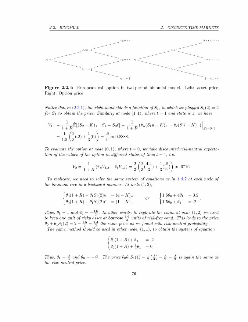
2.2. BINOMIAL 2. DISCRETE-TIME MARKETS
S0 = 1
S1(2) = 2
S1(1) = 12
S2(3) = 4
S2(2) = 1
S2(1) = 14
V0
V1,2
V1,1
(4 − K)+ = 3.2
(1 − K)+ = .2
( 14
− K)+ = 0
Figure 2.2.4: European call option in two-period binomial model. Left: asset price.Right: Option price
Notice that in (2.2.1), the right-hand side is a function of S1, in which we plugged S1p2q “ 2for S1 to obtain the price. Similarly at node p1, 1q, where t “ 1 and state is 1, we have
V1,1 “1
1 ` RErpS2 ´ Kq` | S1 “ S0ℓs “
11 ` R
pπupS1u ´ Kq` ` πℓpS1l ´ Kq`q
ˇ
ˇ
ˇ
S1“S0ℓ
“1
1.5
ˆ
23
p.2q `13
p0q
˙
“.89
« 0.8888.
To evaluate the option at node p0, 1q, where t “ 0, we take discounted risk-neutral expecta-tion of the values of the option in different states of time t “ 1, i.e.
V0 “1
1 ` RpπuV1,2 ` πℓV1,1q “
23
ˆ
23
p4.43
q `13
p.89
q
˙
« .6716.
To replicate, we need to solve the same system of equations as in 1.3.7 at each node ofthe binomial tree in a backward manner. At node p1, 2q,
#
θ0p1 ` Rq ` θ1S1p2qu “ p4 ´ Kq`
θ0p1 ` Rq ` θ1S1p2qℓ “ p1 ´ Kq`
or
#
1.5θ0 ` 4θ1 “ 3.21.5θ0 ` θ1 “ .2
.
Thus, θ1 “ 1 and θ0 “ ´1.63 . In other words, to replicate the claim at node p1, 2q we need
to keep one unit of risky asset at borrow 1.63 units of risk-free bond. This leads to the price
θ0 ` θ1S1p2q “ 2 ´ 1.63 “ 4.4
3 the same price as we found with risk-neutral probability.The same method should be used in other node, p1, 1q, to obtain the system of equation
#
θ0p1 ` Rq ` θ1 “ .2θ0p1 ` Rq ` 1
4θ1 “ 0.
Thus, θ1 “ .83 and θ0 “ ´ .4
9 . The price θ0θ1S1p1q “ 12`
.83˘
´ .49 “ .8
9 is again the same asthe risk-neutral price.
76

2. DISCRETE-TIME MARKETS 2.2. BINOMIAL
At node 0, the replicating portfolio needs to reach the target prices of the claim at timet “ 1, i.e.
#
θ0 ` θ1S0u “ V1,2 “ 4.43
θ0 ` θ1S0ℓ “ V1,1 “ .89
or
#
θ0p1 ` Rq ` 2θ1 “ 4.43
θ0p1 ` Rq ` 12θ1 “ .8
9.
By solving the above system we obtain θ1 “ 24.827 units of risky asset and θ0 “ ´20
81 units ofrisk-free bond in the replicating portfolio. This is the structure of the replicating portfolio atthe beginning of the replication. If the price moves up, we have to restructure the portfolioto keep one unit of risky asset and ´1.6
3 units of risk-free bond. If it moves down, we needto readjust the position to .8
3 units of risky asset and ´ .49 units of risk-free bond.
Pricing European contingent claims in binomial model
Next, consider a general European claim with payoff gpST q, where g : R` Ñ R is a functionwhich assigns a value to the payoff based on the price ST of the asset at terminal time T .Such European claims are also called Markovian claims. Let V0, ..., VT be random variablesrepresenting price of this European claim at time t “ 0, ..., T , respectively. Then, in orderto avoid arbitrage, the derivative price must remain martingale, i.e.
Vt “1
1 ` RErVt`1 | St, ..., S0s.
On the other hand, it follows from the Markovian property of the binomial model thatErVt`1 | St, ..., S0s “ ErVt`1 | St and therefore
Vt “1
1 ` RErVt`1 | Sts.
In other words, the random variable Vt is a function of pt, Stq denoted by
Vt “ V pt, Stq :“ 11 ` R
ErVt`1 | Sts (2.2.2)
Therefore, one needs to evaluate function V pt, Sq shown in Figure 2.2.5.
Notice that by tower property of the conditional expectation, we can write
V pT ´ 2, ST ´2q :“ 11 ` R
ErV pT ´ 1, ST ´1q | ST ´1s
“1
p1 ` Rq2 ErErgpST q | ST ´1, ST ´2s | ST ´2s “1
p1 ` Rq2 ErErgpST q | ST ´2s.
77

2.2. BINOMIAL 2. DISCRETE-TIME MARKETS
V0
V (1, S1,2)
V (1, S1,1)
V (2, S2,3)
V (2, S2,2)
V (2, S2,1)
V (3, S3,4)
V (3, S3,3)
V (3, S3,2)
V (3, S3,1)
g(S0uT )
g(S0uT−1ℓ)
g(S0uT−2ℓ2)
...
g(S0u2ℓT−2)
g(S0uℓT−1)
g(S0ℓT )
V1
V2
V3
VT = g(ST )
Figure 2.2.5: The price of a European contingent claim in binomial model
In addition, if we have
V pt ` 1, St`1q “1
p1 ` RqT ´pt`1qErErgpST q | St`1s
78

2. DISCRETE-TIME MARKETS 2.2. BINOMIAL
Then,
V pt, Stq :“ 11 ` R
ErV pt ` 1, St`1q | St`1s
“1
p1 ` RqT ´tErErgpST q | St`1, Sts | Sts “
1p1 ` RqT ´t
ErErgpST q | Sts.
Therefore, for any t “ 0, ..., T ´ 1, we have
V pt, Stq “1
p1 ` RqT ´tErgpST q | Sts (2.2.3)
Remark 2.2.1. Since binomial model is time-homogeneous, ErgpST q | St “ Ss in (2.2.3)is equal to
ErgpST ´tq | S0 “ Ss.
This suggest that the the price function V pt, Sq in (2.2.2) is a function of S and time-to-maturity τ :“ T ´ t, i.e., V pτ, Sq. Time-to-maturity is often use instead of time infinancial literature of pricing contingent claims.
Replication of European option in the binomial model
To replicate the payoff gpST q at time t ` 1, one needs to solve the following system ofequations
#
θ0p1 ` Rq ` θ1St`1pi ` 1q “ V pt ` 1, St`1pi ` 1qq
θ0p1 ` Rq ` θ1St`1piq “ V pt ` 1, St`1pi ` 1qq.
The solution is given by
θ1 “Vt`1,i`1 ´ Vt`1,i
St`1pi ` 1q ´ St`1piq“
V pt ` 1, Stpiquq ´ V pt ` 1, Stpiqlq
Stpiqpu ´ ℓq
which is the number of units of risky asset in the replicating portfolio and
θ0 “uVt`1,i ´ lVt`1,i`1
pu ´ ℓqp1 ` Rq“
uV pt ` 1, Stpiqlq ´ lV pt ` 1, Stpiquq
pu ´ ℓqp1 ` Rq
which is the number of units of risk-free bond in the replicating portfolio. In other words,the replicating portfolio is a self-financing portfolio given by (2.1.3) with w0 “ V0 andportfolio strategy given by ∆p0, S0q, ..., ∆pT ´ 1, ST ´1q
∆pt, Sq :“ V pt ` 1, Suq ´ V pt ` 1, Sℓq
Spu ´ ℓq. (2.2.4)
79

2.2. BINOMIAL 2. DISCRETE-TIME MARKETS
The number of units of risky asset in the replicating portfolio, given by (2.2.4), is calledthe Delta of the contingent claim at time t. Basically, the Delta of a European Markoviancontingent claim is a function of price on underlying asset given by (2.2.4).
Remark 2.2.2. As you can see from (2.2.4), Delta of the contingent claim at time tmeasures the sensitivity of the value of the contingent claim with respect to the changesin the underlying price, i.e., changes in the price of option due to changes in the price ofunderlying.
By (2.1.3), the replicating portfolio for the binomial model takes the form
V pt, Stq “ V p0, S0q ` Rt´1ÿ
i“0pV pi, Siq ´ ∆pi, SiqSiq `
t´1ÿ
i“0∆pi, SiqpSi`1 ´ Siq,
where V pi, Siq is the price of contingent claim at time i when the underlying price is Si.The term R
řt´1i“0pV pi, Siq´∆ipSiqSiq represents accumulated changes in the risk-free bond
part of replicating portfolio caused by interest rate, andřt´1
i“0 ∆ipSiqpSi`1 ´ Siq representsthe accumulated changes in the replicating portfolio caused by the changes in the riskyasset price. The act of constructing replicating portfolio for a contingent claim is ofterreferred to as Delta hedging.The above discussion is summarized in the following algorithm.
Backward pricing and replicating European options in binomial model1: At time T , the value of the option is gpST pjqq.2: for each t “ T ´ 1, ..., 0 do3: for each j “ 1, ..., t ` 1 do4: The value of the option V pt, Stpjqq “ 1
1`R ErV pt ` 1, St`1q | St “ Stpjqs.5: The replicating portfolio is made of ∆pt, Stpjqq units of risky assets and V pt, Stpjqq ´
Stpjq∆pt, Stpjqq is risk-free bond.6: end for7: end for
Remark 2.2.3. Give functions ∆ and V are calculated, one has to plug in time t andasset price St into the function to find the price and adjust the replicating portfolio of thecontingent claim. However, there is no guarantee that the quoted prices in the market matchthe prices in the binomial (or any other) model. In such case, interpolation techniques canbe exploited to fine the price and adjust the replicating portfolio.
Exercise 2.2.2. In the binomial model, show that the Delta of a call option ∆call and theDelta of a put option ∆put with the same maturity and strike satisfy
∆callt ´ ∆put
t “ 1, for all t “ 0, ..., T ´ 1.
80

2. DISCRETE-TIME MARKETS 2.2. BINOMIAL
Is this result model-independent? Hint: put-call parity.
Exercise 2.2.3. Consider a two-period binomial model for a risky asset with each periodequal to a year and take S0 “ $1, u “ 1.03 and ℓ “ 0.98.
a) If the interest rate for both periods is R “ .01, find the price of the option with thepayoff shown in Figure 2.2.6 with K1 “ 1.00 and K2 “ 1.05 at all nodes of the tree.
K1 K2
K2 −K1
ST
g(ST )
Figure 2.2.6: Payoff of Exercise 2.2.3
b) Find the replicating portfolio at each node of the tree.
Exercise 2.2.4. Consider a two period binomial model for a risky asset with each periodequal to a year and take S0 “ $1 u “ 1.05 and ℓ “ 1.00. Each year’s interest rate comesfrom Exercise 1.1.4.
a) Is there any arbitrage? Why? Give one arbitrage portfolio.Now consider a two period binomial model for a risky asset with each period equal toa year and take S0 “ $1 u “ 1.05 and ℓ “ 0.95.
b) Find the price of the option with the payoff shown in Figure 1.1.6 with K1 “ 1.00and K2 “ 1.05 at all nodes of the tree. Find the interest rates for each period frominformation in part (a).
c) Find the replicating portfolio and specifically ∆ at all nodes of the tree.
Remark 2.2.4. 2.2.2 suggest that the price of a Markovian claim in Binomial model doesnot depend on the past movements of the price and it only depends on the current price S.This is not indeed true for nonMarkovian claims. For example a look-back option with pay-off pmaxt“0,...,T St ´ Kq
`or Asian option
´
1T `1
řTt“0 St ´ K
¯
`are nonMarkovian options
with the price which depends to some extent in the past history of the price movement ratherthan only the current price of the underlying. See for instance Exercise 2.2.5. Evaluationof these type of nonMarkovian payoffs, a.k.a. path-dependent payoffs, cannot benefit fullyfrom the Markovian property of the model.
81
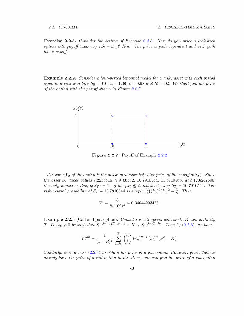
2.2. BINOMIAL 2. DISCRETE-TIME MARKETS
Exercise 2.2.5. Consider the setting of Exercise 2.2.3. How do you price a look-backoption with payoff pmaxt“0,1,2 St ´ 1q
`? Hint: The price is path dependent and each path
has a payoff.
Example 2.2.2. Consider a four-period binomial model for a risky asset with each periodequal to a year and take S0 “ $10, u “ 1.06, ℓ “ 0.98 and R “ .02. We shall find the priceof the option with the payoff shown in Figure 2.2.7.
0 10 11 12
1
ST
g(ST )
Figure 2.2.7: Payoff of Example 2.2.2
The value V0 of the option is the discounted expected value price of the payoff gpST q. Sincethe asset ST takes values 9.2236816, 9.9766352, 10.7910544, 11.6719568, and 12.6247696,the only nonzero value, gpST q “ 1, of the payoff is obtained when ST “ 10.7910544. Therisk-neutral probability of ST “ 10.7910544 is simply
`24˘
pπuq2pπℓq2 “ 3
8 . Thus,
V0 “3
8p1.02q4 « 0.34644203476.
Example 2.2.3 (Call and put option). Consider a call option with strike K and maturityT . Let k0 ě 0 be such that S0uk0´1lT ´k0`1 ă K ď S0uk0 lT ´k0. Then by (2.2.3), we have
V call0 “
1p1 ` RqT
Tÿ
k“k0
ˆ
n
k
˙
pπuqn´k
pπℓqk
pSkT ´ Kq.
Similarly, one can use (2.2.3) to obtain the price of a put option. However, given that wealready have the price of a call option in the above, one can find the price of a put option
82
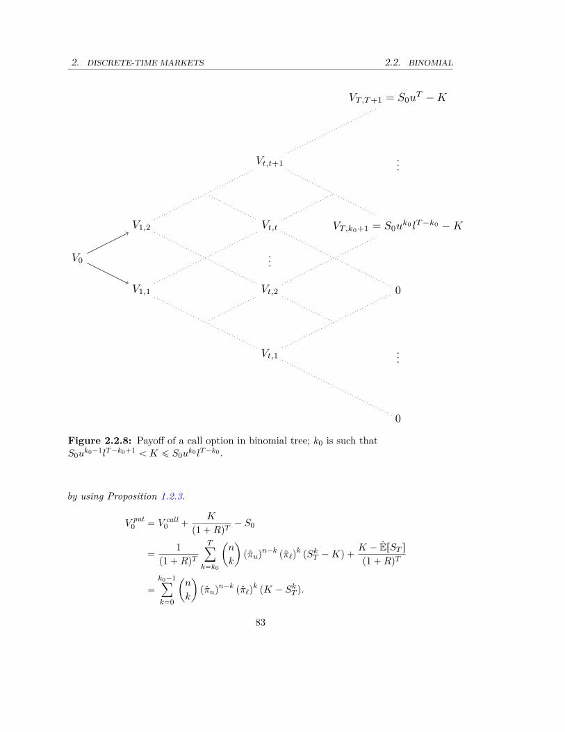
2. DISCRETE-TIME MARKETS 2.2. BINOMIAL
V0
V1,2
V1,1
Vt,t+1
Vt,t
...
Vt,2
Vt,1
VT,T+1 = S0uT −K
...
VT,k0+1 = S0uk0 lT−k0 −K
0
...
0
Figure 2.2.8: Payoff of a call option in binomial tree; k0 is such thatS0uk0´1lT ´k0`1 ă K ď S0uk0 lT ´k0 .
by using Proposition 1.2.3.
V put0 “ V call
0 `K
p1 ` RqT´ S0
“1
p1 ` RqT
Tÿ
k“k0
ˆ
n
k
˙
pπuqn´k
pπℓqk
pSkT ´ Kq `
K ´ ErST s
p1 ` RqT
“
k0´1ÿ
k“0
ˆ
n
k
˙
pπuqn´k
pπℓqk
pK ´ SkT q.
83

2.2. BINOMIAL 2. DISCRETE-TIME MARKETS
In the above, we used martingale property of discounted asset price, (2.1.4), to write S0 “
ErST s “ErST s
p1`RqT and we expanded the expectation as
K ´ ErST s “ ErK ´ ST s “
Tÿ
k“0
ˆ
n
k
˙
pπuqn´k
pπℓqk
pK ´ SkT q.
2.2.4 Dividend paying stock
Stock usually pays cash dividend to the share holders. Then, it is on the individual shareholders to decide whether to consume the cash divided or invest it back into the market.The dividend policy is decided by the management of the company but it is also influencedby the preference of the share holders. The dividend is usually expressed as a percentageof the asset price, which is referred to as dividend yield. If the asset price at time t is St,then after paying dt P r0, 1q portion of asset price as dividend, the asset price is reducedto p1 ´ dtqSt. Therefore, under the dividend policy d1, ..., dn, the asset price dynamics inbinomial model follows
St “ S0H1...Ht
tź
i“1p1 ´ diq,
where Hi is a sequence of i.i.d. random variables with distribution
PpHi “ uq “1 ` R ´ ℓ
u ´ ℓand PpHi “ ℓq “
u ´ 1 ´ R
u ´ ℓ.
If we define Hi “ Hip1 ´ diq, the dividend policy makes the binomial model look like
St “ S0H1...Ht.
See Figure 2.2.9. Then, Hi is distributed as
PpHi “ up1 ´ diqq “1 ` R ´ ℓ
u ´ ℓand PpHi “ ℓp1 ´ diqq “
u ´ 1 ´ R
u ´ ℓ.
Remark 2.2.5. It is important to notice that in this case, the no-arbitrage conditionremains the same as in the case when the underlying asset does not pay any dividend, i.e.,ℓ ă 1 ` R ă u. However, the dynamics of the dividend paying underlying asset is different.
One way of pricing contingent claims on dividend paying asset is to introduce an adjustedasset price with no dividend and transform the payoff in terms of the adjusted asset price.If we define the adjusted asset price by St :“ S0H1...Ht, then St “ St
śTi“1p1 ´ diq. Then,
the payoff of a European contingent claim given by gpST q is given in terms of ST byg`
STśT
i“1p1 ´ diq˘
on the adjusted binomial asset ST . Then, the pricing of a contingent
84

2. DISCRETE-TIME MARKETS 2.2. BINOMIAL
S0
S0u(1 − d1)
S0ℓ(1 − d1)
S0u2(1 − d1)(1 − d2)
S0uℓ(1 − d1)(1 − d2)
S0ℓ2(1 − d1)(1 − d2)
S0u3(1 − d1)(1 − d2)(1 − d3)
S0u2ℓ(1 − d1)(1 − d2)(1 − d3)
S0uℓ2(1 − d1)(1 − d2)(1 − d3)
S0ℓ3(1 − d1)(1 − d2)(1 − d3)
S0un(1 − d1)...(1 − dn)
S0un−1ℓ(1 − d1)...(1 − dn)
S0un−2ℓ2(1 − d1)...(1 − dn)
.
.
.
S0u2ℓn−2(1 − d1)...(1 − dn)
S0uℓn−1(1 − d1)...(1 − dn)
S0ℓn(1 − d1)...(1 − dn)
Figure 2.2.9: Dividend paying asset in binomial model
claim with payoff gpST q at time t given St “ S is given by
V pt, Sq :“ 1p1 ` RqT ´t
ErgpST q | St “ Ss “1
p1 ` RqT ´tE”
g`
ST
Tź
j“t`1p1 ´ diq
˘
| St “ Sı
“1
p1 ` RqT ´t
Tÿ
i“t
ˆ
T ´ t
i
˙
πiuπT ´t´i
ℓ g´
SuiℓT ´t´iTź
j“t`1p1 ´ djq
¯
.
(2.2.5)
Remark 2.2.6. Notice that the price V pt, Sq of a European contingent claim gpST q on a
85

2.3. CALIBRATING THE PARAMETERS OF THE MODEL TO THE MARKETDATA: BINOMIAL MODEL 2. DISCRETE-TIME MARKETS
dividend-paying underlying asset S is no longer a function of time-to-maturity τ “ T ´ t.This is due to the term
śTj“t`1p1 ´ diq in (2.2.5) which cannot be expressed as a function
of τ , unless di “ d for all i “ 1, ..., T , thenśT
j“t`1p1 ´ diq “ p1 ´ dqτ
Exercise 2.2.6. Consider a two-period binomial model for a risky asset with each periodequal to a year and take S0 “ $1, u “ 1.15 and ℓ “ 0.95. The interest rate for both periodsis R “ .05.
a) If the asset pays 10% divided yield in the first period and 20% in the second period,find the price of a call option with strike K “ .8.
b) Consider a more complicated dividend strategy which pays 10% divided yield only ifthe price moves up and no dividend if the price moves down at each period. Find theprice of a call option with strike K “ .8.
Remark 2.2.7. Assume that the divided strategy is random, i.e., at each node of thebinomial tree at time t and state j, the divided is a random variable dpt, jq, for j “ 1, ..., t`1.The two-period binomial model in Exercise 2.2.6 part (b), is a special case of this case whenpricing is not a difficult job.In general, even for a Markovian asset price model and a Markovian contingent claims
gpST q, the pricing is similar to pricing a path dependent option if the dividend strategy ispath dependent. This is because the modified payoff takes the form g
`
STśT
t“1p1´dpt, jtqq˘
,where j1, ..., jT determines the path of the price from 0 to T . Therefore, pricing and hedgingmust be conducted similar to Remark 2.2.4 and Exercise 2.2.5.
2.3 Calibrating the parameters of the model to the marketdata: Binomial model
Calibration is the practice of matching the parameter of a model to the data. In binomialmodel, the parameters are interest rate R, u and ℓ. Calibrating the risk-free interest rateR is a separate job and usually uses the price quotes of the risk-free (sovereign) bonds. Forthe purpose of this section, we assume that the yield of a zero bond is already calibratedand satisfies Rtpt ` δq “ rδ ` opδq, where short rate r is constant and δ is the duration ofone period in the binomial market.
Data: price quote and return
Assume that the asset price quotes are collected at δ time lapse, i.e., S´mδ, ..., S0 be thepast quotes of the asset price from time ´mδ until now t “ 0. We denote the quoted priceby S to distinguish it from the random variable S for future price.
86

2. DISCRETE-TIME MARKETS 2.3. CALIBRATION
The arithmetic return and the logarithmic return at time t are defined by
Rartht :“ St`δ ´ St
St,
andRlog
t :“ lnˆ
St`δ
St
˙
,
respectively. If the time step δ is small, then the price movement St`δ ´ St is also small,then Rlog
t and Rartht are very close8. However, we will see that the small difference between
the two returns will show up in parameter estimation. For the moment, we focus on thearithmetic return and drop the superscript "arth" for simplicity. We discuss the logarithmicreturn (or log return) at the end of this section.From the data points S´mδ, ..., S0, we obtain data points for the return, i.e., R´mδ, ..., R´δ
given by
R´kδ “Sp´k`1qδ ´ S´kδ
S´kδ
.
Next, we will use this date to estimate some parameters of the market which are importantin the calibration process.
Binomial model with physical probability
The price quote data is coming from the physical probability and not the risk-neutralprobability; see Remark 1.3.5. Therefore for calibration, we need to present the binomialmodel with physical probability rather than the risk-neutral probability. While the nodesof the binomial model will not change, the probability must change; St`1 “ StHt`1 andtHtu
8t“1 is a sequence of i.i.d. random variables with the following distribution under
physical measure
Ht “
#
u with probability p
ℓ with probability 1 ´ p, for all t “ 0, 1, ....
Notice that in physical binomial model the sequence of return tRtu8t“0 are also making
a sequence of i.i.d. random variables. So, to proceed with calibration, we need to imposethe same assumption on the data.
Assumption 2.3.1. The return tRtu8t“0 is a sequence of i.i.d. random variables with
mean and the variance given by by µδ ` opδq and σ2δ ` opδq, respectively.
The dimension-less quantities σ and µ are respectively called the volatility and meanreturn rate of the price.
8lnp1 ` xq « x for small x
87
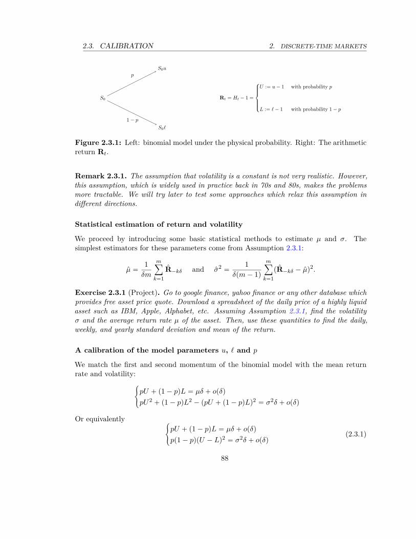
2.3. CALIBRATION 2. DISCRETE-TIME MARKETS
S0
S0u
S0ℓ
p
1− p
Rt = Ht − 1 =
U := u− 1 with probability p
L := ℓ− 1 with probability 1− p
Figure 2.3.1: Left: binomial model under the physical probability. Right: The arithmeticreturn Rt.
Remark 2.3.1. The assumption that volatility is a constant is not very realistic. However,this assumption, which is widely used in practice back in 70s and 80s, makes the problemsmore tractable. We will try later to test some approaches which relax this assumption indifferent directions.
Statistical estimation of return and volatility
We proceed by introducing some basic statistical methods to estimate µ and σ. Thesimplest estimators for these parameters come from Assumption 2.3.1:
µ “1
δm
mÿ
k“1R´kδ and σ2 “
1δpm ´ 1q
mÿ
k“1pR´kδ ´ µq2.
Exercise 2.3.1 (Project). Go to google finance, yahoo finance or any other database whichprovides free asset price quote. Download a spreadsheet of the daily price of a highly liquidasset such as IBM, Apple, Alphabet, etc. Assuming Assumption 2.3.1, find the volatilityσ and the average return rate µ of the asset. Then, use these quantities to find the daily,weekly, and yearly standard deviation and mean of the return.
A calibration of the model parameters u, ℓ and p
We match the first and second momentum of the binomial model with the mean returnrate and volatility:
#
pU ` p1 ´ pqL “ µδ ` opδq
pU2 ` p1 ´ pqL2 ´ ppU ` p1 ´ pqLq2 “ σ2δ ` opδq
Or equivalently#
pU ` p1 ´ pqL “ µδ ` opδq
pp1 ´ pqpU ´ Lq2 “ σ2δ ` opδq(2.3.1)
88
2. DISCRETE-TIME MARKETS 2.3. CALIBRATION
In the above system of two equations, there are three unknowns U , L and p, which givesus one degree of freedom. We are going to use this degree of freedom by assuming thatthe variance of return Rt under risk-neutral probability is also σ2δ, i.e.
πuπℓpU ´ Lq2 “ σ2δ ` opδq,
where πu “ 1`R´ℓu´ℓ “ R´L
U´L9. To simplify further, we also drop the opδq term from the
equations. Therefore, we have a system of three equations and three unknown.$
’
&
’
%
pU ` p1 ´ pqL “ µδ
pp1 ´ pqpU ´ Lq2 “ σ2δ
pU ´ RqpR ´ Lq “ σ2δ
For the sake of simplicity, we set new variables
α “U ´ R?
δσ, β “
R ´ L?
δσ, and r “
R
δ, (2.3.2)
where r is the annual interest rate (APR) calculated at periods δ. Thus, we have$
’
&
’
%
pα ´ p1 ´ pqβ “ λ?
δa
pp1 ´ pqpα ` βq “ 1αβ “ 1
(2.3.3)
Here λ :“ µ´rσ .
Remark 2.3.2 (Risk premium). The quantity µ´rσ is referred to as risk premium of the
asset and measures the excess mean return of the asset adjusted with its level of riskinessmeasured by the volatility.
The solution of (2.3.3) is given by
α “
c
1 ´ p
p` λ
?δ, β “
c
p
1 ´ p´ λ
?δ, and p “
11 ` x2
0(2.3.4)
where x0 is the unique positive solution of equation (see Figure 2.3.2)
x ´1x
“ λ?
δ. (2.3.5)
9The reason behind this choice, will be more clear later when we study continuous time models, specifi-cally Black-Scholes model.
89

2.3. CALIBRATION 2. DISCRETE-TIME MARKETS
x0
λ√δ
x
x− x−1
Figure 2.3.2: Positive solution of equation x ´ 1x “ λ
?δ.
Then, u, ℓ are given by
u “ 1 ` δr `?
δσα, and ℓ “ 1 ` δr ´?
δσβ. (2.3.6)
Remark 2.3.3. The above calibration is robust in the sense that for any possible value ofparameters σ ą 0, µ and r, one can find proper u and ℓ such that ℓ ă 1 ` R ă u in aunique fashion. Notice that in (2.2.3), pricing contingent claims is not affected by p andthus, p is a least important parameter in this context.
Example 2.3.1. Symmetric probability We shall show that the following choice of param-eters for the binomial model also provides a calibration, i.e., it satisfies the Assumption2.3.1.
u “ eδpr´ σ22 q`
?δσ, ℓ “ eδpr´ σ2
2 q´?
δσ and p “12
´
1 ` λ?
δ¯
.
First notice that
Rt “
$
&
%
eδpr´ σ22 q`
?δσ ´ 1 with probability 1
2
´
1 ` λ?
δ¯
eδpr´ σ22 q´
?δσ ´ 1 with probability 1
2
´
1 ´ λ?
δ¯
Therefore,
ErRts “12
ˆ
´
eδpr´ σ22 q`
?δσ ´ 1
¯´
1 ` λ?
δ¯
`
´
eδpr´ σ22 q´
?δσ ´ 1
¯´
1 ´ λ?
δ¯
˙
.
90
2. DISCRETE-TIME MARKETS 2.3. CALIBRATION
We use ex “ 1 ` x ` x2
2! ` x3
3! ` ¨ ¨ ¨ , to write
ErRts “12
ˆ
´
δpr ´σ2
2q `
?δσ `
δσ2
2` opδq
¯´
1 ` λ?
δ¯
`
´
δpr ´σ2
2q ´
?δσ `
δσ2
2` opδq
¯´
1 ´ λ?
δ¯
˙
“δpr ´σ2
2`
σ2
2` λσq ` opδq “ µδ ` opδq
Recall that λσ “ µ ´ r. On the other hand,
ErR2t s “
12
ˆ
´
eδpr´ σ22 q`
?δσ ´ 1
¯2´1 ` λ
?δ¯
`
´
eδpr´ σ22 q´
?δσ ´ 1
¯2´1 ´ λ
?δ¯
˙
“12
ˆ
´
δσ2 ` opδq
¯´
1 ` λ?
δ¯
`
´
δσ2 ` opδq
¯´
1 ´ λ?
δ¯
˙
“ σ2δ ` opδq.
Exercise 2.3.2. Show that the following choice of parameters for the binomial model alsoprovides a calibration, i.e., it satisfies the Assumption 2.3.1.
u “ eδν`?
δσ, ℓ “ eδν´?
δσ and p “12
´
1 ``µ ´ ν
σ´
σ
2˘
?δ¯
,
where ν is a real number. Find the range of ν in terms of other parameters such that thereis no arbitrage.
Calibration for option pricing
Approximating the rate of return µ is often a more difficult task than the volatility. Meth-ods such as CAPM10 has developed to approximate the rate of return. However, if thecalibration is only used for option pricing, we often do not need the rate of return. Recallthat under risk-neutral probability, the return of a binomial asset is equal to the zero bondyield;
ErRts “ ErHt ´ 1s “ pu ´ 1qπu ` pℓ ´ 1qπℓ “pu ´ 1qp1 ` R ´ ℓq ` pℓ ´ 1qpu ´ 1 ´ Rq
u ´ ℓ“ R.
Therefore, if we only calibrate the binomial model under risk-neutral probability, the rateof return under physical probability is irrelevant.We impose the following assumption of the risk-neutral distribution of the return process
and use it to calibrate the binomial model under risk-neutral probability by the data onthe volatility only.
10Capital asset pricing method
91
2.3. CALIBRATION 2. DISCRETE-TIME MARKETS
Assumption 2.3.2. The arithmetic return tRartht ut is a sequence of independent random
variables under risk-neutral probability P with mean ErRts “ rδ ` opδq and ˆvarpRtq “
σ2δ ` opδq.
Given R “ rδ ` opδq, we have ErRts “ rδ ` opδq and therefore, the only equation that weobtain is
pU ´ RqpR ´ Lq “ σ2δ.
Here, we drop opδq term for simplicity. If we define α “ U´R?δσ
and β “ R´L?δσ
, we haveαβ “ 1.
Time-varying return and volatility
Assumption 2.3.1, tRtut is a sequence of i.i.d. random variables, is not realistic in somesituations and must be relaxed. Several empirical studies show that the volatility is not con-stant. This removes the "identical distribution" of the return sequence. The independencecondition also does not have an empirical basis. In this section, we keep the independenceassumption, but remove the identically distributed on tRtut.
Assumption 2.3.3. The arithmetic return tRartht ut is a sequence of independent random
variables with mean ErRts “ µtδ ` opδq and varpRtq “ σ2t δ ` opδq.
Assumption 2.3.3 allows for the parameters µ and σ to vary over time. To see more detailson the estimation of time-varying parameters, see [16]. In addition, we can also allow forinterest rate to depend of time Rt “ rtδ. Therefore, the calibration in the previous section,Section 2.3, should be modified in the way that α, β, and p are time varying, and satisfy
$
’
&
’
%
ptαt ´ p1 ´ ptqβt “ λt
?δ
a
ptp1 ´ ptqpαt ` βtq “ 1αtβt “ 1
Here λt :“ µt´rt
σt. (2.3.4) and (2.3.5) also become time-varying and we have
ut “ 1 ` δrt `?
δσtαt, and ℓt “ 1 ` δrt ´?
δσtβt. (2.3.7)
92

3. CONTINUOUS MARKETS
3
Modeling financial assets incontinuous-time
Louis Bachelier in 1900, [3], introduced the first asset price model and pricing methodfor the derivatives. Although this model is now considered impractical, the educationalimplications of this model is still important. Bachelier modeled the discounted asset priceby a Brownian motion. As seen in Section B.5, Brownian motion is weak limit of normalizedrandom walk. At the time of Bachelier, the Brownian motion was not even rigorouslydefined. However, many properties of Brownian motion was well understood. Bacheliercontribution in the theory of probability and stochastic processes is to use heat equationin derivative pricing. His contribution was undermined for about 30 years until NikolaiKolmogorov who partial differential equations to describe a class of stochastic processes,called diffusion processes. Nikolai Kolmogorov is the first mathematician who broughtprobability into rigor by establishing its mathematical foundation. Other mathematiciansbuilt up on Kolmogorov’s work; Norbert Wiener was the first to define Brownian motion,and Kyiosi (read Kiyoshi) Itô introduced a simple representation of diffusion processes interms of Brownian motion.
In finance, the Bachelier model has been out of record for more than 50 years. PaulSamuelson suggested Geometric Brownian motion (GBM), which never takes nonpositivevalues, to model the asset price. GBM is also known as Black-Scholes model, names afterFischer Black and Myron Scholes. Black and Scholes in [6] and Robert Merton in [25]independently developed a pricing method for derivatives based on GBM. For a throughreview of Bachelier’s effort and contribution see [30]. For a brief history of asset pricemodels see [28]. For the biography of Bachelier see [33].
93
3.1. TRADING AND ARBITRAGE IN CONTINUOUS-TIME MARKETS3. CONTINUOUS MARKETS
3.1 Trading and arbitrage in continuous-time markets
Recall form Section II.2.1 that in a discrete-time market where trading occurs at times t0 “
0 ă t1 ă ... ă tN “ T the value of the portfolio generated by the strategy ∆0, ∆t1 , ..., ∆tN´1
is given by
Wtn “ W0 `
n´1ÿ
i“0RipWti ´ ∆tiStiq `
n´1ÿ
i“0∆tipSti`1 ´ Stiq.
Here Ri is the interest rate for the period of time rti, ti`1s which can be taken to berpti`1 ´ tiq. For i “ 0, ..., N ´ 1, the strategy ∆ti is a function of the history asset price,i.e., Su for u ď ti. Therefore,
Wtn “ W0 ` rn´1ÿ
i“0pWti ´ ∆tiStiqpti`1 ´ tiq `
n´1ÿ
i“0∆tipSti`1 ´ Stiq.
If we take ti`1 ´ ti :“ δ “ TN and let δ Ñ 0, we obtain the Reimann integral
limδÑ0
rN´1ÿ
i“0pWti ´ ∆tiStiqpti`1 ´ tiq “ r
ż T
0pWt ´ ∆tStqdt,
which is the accumulated net change in the portfolio due to investment on the risk-freeasset. The limit of the second term
n´1ÿ
i“0∆tipSti`1 ´ Stiq
does not necessarily exist unless we enforce proper assumptions on the asset price S. Forinstance if the asset price follows Brownian motion (Bachelier model) or GBM (Black-Scholes model), then the limit exists and is interpreted as stochastic Itô integral. Giventhe stochastic integral above is well-defined, the wealth generated by the trading strategyt∆utě0 follows
Wt “ W0 ` r
ż t
0pWs ´ ∆sSsqds `
ż t
0∆sdSs. (3.1.1)
We choose the same notion p∆ ¨ Sqt :“şt0 ∆sdSs for the stochastic integral in continuous-
time. Notice that in the discrete-time setting, the strategy ∆ at time ti is the function ofthe past history of asset price S0, ..., Sti . When we pass to the limit, the trading strategyat time t, ∆t, depends only on the paths of asset until time t, i.e., tSu : u ď tu. In otherwords, a trading strategy does not use any informations from the future.Following the discussion in Section C.1, specifically (C.1), the stochastic integral is defined
only in the almost surely sense and can only be defined on the sample paths of the assetprice model S. Therefore, a probability space pΩ,Pq (or at least the set of sample paths of
94

3. CONTINUOUS MARKETS 3.2. CONTINUOUS-TIME MARKET OF BACHELIER
the asset price) is needed. Then, the notion of arbitrage is define das follows:
Definition 3.1.1. A (weak) arbitrage opportunity is a portfolio ∆ such that
a) W0 “ 0,
b) WT ě 0, and
c) WT ą 0 of a set of sample paths with positive P probability.
A strong arbitrage opportunity is a portfolio ∆ such that
a) W0 ă 0,
b) WT ě 0, and
Given the stochastic integral p∆ ¨ Sqt “şt0 ∆sdSs is defined in a probability space pΩ,Pq,
the fundamental theorem of asset pricing (FTAP) for continuous-time is as follows. Twoprobabilities P and P are called equivalent if any event with probability zero under one ofthem has probability zero under the other, i.e., PpAq “ 0 if and only if PpAq “ 0.
Theorem 3.1.1 (Fundamental theorem of asset pricing (FTAP)). There is no weak ar-bitrage opportunity in the continuous-time model if and only if there exist a probability P,a.k.a. risk-neutral probability, equivalent to P such that S is a P-(local) martingale1.In addition, the market is complete if and only if there is only there is a unique risk-neutral
probability.
Recall that a market model is called complete if any contingent claim is replicable, i.e.,for any payoff XT which is a function over all paths tSu : u ď T u of the asset price untiltime T , there exists a strategy ∆ :“ t∆tu
Tt“0 such that the wealth W generated by ∆ in
(3.1.1) satisfies XT “ WT .
Theorem 3.1.2 (Fundamental theorem of asset pricing (FTAP)). Under the same settingas in Theorem 3.1.1, the market is complete if and only if there is only there is a uniquerisk-neutral probability.
3.2 Continuous-time market of BachelierWe start with recalling the properties of a Brownian motion from Section B.5. A Brownianmotion is a stochastic process characterized by the following properties.
1) B has continuous sample paths,
2) B0 “ 0,1local martingale is roughly a martingale without condition (a) in Definition B.13.
95

3.2. BACHELIER MODEL 3. CONTINUOUS MARKETS
3) when s ă t, the increment Bt ´ Bs is a normally distributed random variables withmean 0 and variance t ´ s and is independent of Bu; for all u ď s.
The Bachelier model is based on an assumption made by Bachelier himself in his PhDthesis“Théorie de la spèculation” (Pg 33 [3]):
L’espèrance mathématique de l’acheteur de prime est nulle (3.2.1)
which translates into “Mathematical expectation of the buyer of the asset is zero”. In themodern probabilistic language, what Bachelier meant is that the discounted asset price isa martingale under risk-neutral probability, which implies no-arbitrage condition by theFTAP in [10]. As the simplest martingale in continuous-time, Bachelier model simply takesthe discounted asset price under risk-neutral probability a factor of a standard Brownianmotion, i.e.
St “ e´rtSt “ S0 ` σBt, σ ą 0. (3.2.2)
Therefore under risk-neutral probability, St has Gaussian distribution with constant meanS0 and variance σ2t, i.e., the pdf of St is given by
fStpxq “
1σ
?2πt
expˆ
´px ´ S0q2
2σ2t
˙
for x P R and t ą 0. (3.2.3)
The price of the underlying asset in Bachelier model is given by St “ ertpS0 ` σBtq. Underrisk-neutral probability, St is also a Gaussian random variable with
ErSts “ S0ert, and varpStq “ σ2e2rtt.
Therefore, the risk-neutral expected value of the asset price increases in a similar fashionas a risk-free asset. The variance of St increases exponentially fast too. It follows formapplying Itô formula (C.4) on fpt, xq “ ertpS0 ` σxq that St satisfies the SDE
dSt “ rStdt ` σertdBt. (3.2.4)
Inherited from Brownian motion, Bachelier model possesses the same properties as bino-mial model in Section 2.2.2; i.e.
1) time-homogeneity,
conditional distribution of St given Ss “ S equals distribution ofSt´s with S0 “ S
2) Markovian,
ErfpStq | Su, u ď ss “ ErfpStq | Sss
96
3. CONTINUOUS MARKETS 3.2. BACHELIER MODEL
3) martingale,
ErSt | Su, u ď ss “ Ss.
The conditioning on tSu, u ď su (or Ss) in the above conditional expectations can simplybe replaced by tSu, u ď su (or Ss). Since having the knowledge on the asset price isequivalent of having the knowledge on the discounted asset price. Therefore, we have
Er¨ | Su, u ď ss “ Er¨ | Su, u ď ss (or Er¨ | Sss “ Er¨ | Sss).
It is important for the reader to know that Bachelier model is not practically interestingin modeling financial markets. However, for educational purposes, it has all the basiccomponents of the more practical model of Black-Scholes. In addition, pricing a Europeanoption in Bachelier model is equivalent to solving a heat equation, which on one hand, canalso be used in Black-Scholes model, and on the other hand, is a special case of parabolicpartial differential equations which appear in more general models. Section 3.2.3 discussesthe drawbacks of Black-Scholes model.
3.2.1 Pricing and replicating contingent claims in Bachelier model
As a result of quote (3.2.1), Bachelier concluded that the price of a European contingentclaim with payoff gpST q is simply the discounted expectation of the payoff under risk-neutralprobability, i.e.
V0 “ e´rT ErgpST qs. (3.2.5)
In addition, given the past history of asset price tSu : u ď tu, the price of the option attime t is given by
Vt “ e´rpT ´tqErgpST q | Su : u ď ts. (3.2.6)
For simplicity in the rest of this section, we denote the past history of asset price byFt :“ tSu : u ď tu, i.e.,
Er¨ | Su : u ď ts “ Er¨ | Fts. (3.2.7)
Price of contingent claim at time zero
Since under risk-neutral probability ST “ erT ST is a Gaussian random variable with meanerT S0 and variance e2rT σ2T , one can explicitly calculate V0 in cases where the followingintegral can be given in a closed-form,
V0 “e´rT
σ?
2πT
ż 8
´8
g`
erT x˘
e´px´S0q2
2σ2T dx. (3.2.8)
We start off by providing a closed form for the Bachelier price of a call option.
97

3.2. BACHELIER MODEL 3. CONTINUOUS MARKETS
Example 3.2.1 (Price of call and put in Bachelier model). Let gpST q “ pST ´ Kq` “
erT pST ´Kq`, where K “ e´rT K. Since ST „ NpS0, σ2T q, the price V call0 can be calculated
in closed form.
V call0 “
e´rT
σ?
2πT
ż 8
´8
`
erT x ´ K˘
`e´
px´S0q2
2σ2T dx
“1
σ?
2πT
ż 8
´8
´
x ´ K¯
`e´
px´S0q2
2σ2T dx
“1
σ?
2πT
ż 8
K
´
x ´ K¯
e´px´S0q2
2σ2T dx.
By the change of variable y “ x´S0σ
?T
, we obtain
V call0 “
1?
2π
ż 8
pK´S0qpσ?
T q
´
σ?
Ty ` S0 ´ K¯
e´y22 dy
“σ
?T
?2π
ż 8
pK´S0qpσ?
T q
ye´y22 dy `
S0 ´ K?
2π
ż 8
pK´S0qpσ?
T q
e´y22 dy
The second integral above can be calculated in terms of the standard normal cdf Φpxq “1?2π
şx´8
e´y22dy, i.e.,
1σ
?2πT
ż 8
pK´S0qpσ?
T q
e´y22 dy “ 1 ´ Φ
´K ´ S0
σ?
T
¯
“ Φ´S0 ´ K
σ?
T
¯
.
Notice that here we used Φpxq “ 1 ´ Φp´xq.
The first integral can be evaluated by the change of variable u “y2
2 .
1?
2π
ż 8
pK´S0qpσ?
T q
ye´y22 dy “
1?
2π
ż 8
|S0´K|pσ?
T q
ye´y22 dy
“ ´1
?2π
e´y22
ˇ
ˇ
ˇ
ˇ
8
|S0´K|pσ?
T q
“1
?2π
e´pS0´Kq2
2σ2T “ Φ1´S0 ´ K
σ?
T
¯
,
where Φ1pxq “ 1?2π
e´ x22 is the pdf of standard normal.
To summarize, we have
V call0 “ σ
?T`
Φ1pdq ` dΦpdq˘
, (3.2.9)
98

3. CONTINUOUS MARKETS 3.2. BACHELIER MODEL
where d “ S0´Kσ
?T
. By the put-call parity we have,
V put0 “ K ´ S0 ` V call
0 “ σ?
T`
Φ1pdq ´ dΦp´dq˘
.
Example 3.2.2. A digital option with is an option with payoff
gpST q “ 1tST ěKu
#
1 ST ě K
0 ST ă K.
The Bachelier price of the digital option is given by
V digit0 “ e´rT E
”
1tST ěKu
ı
“ e´rT P´
ST ě K¯
.
Notice that ST ě K is equivalent to Bt?t
ě e´rtK´S0σ
?t
. Since Bt?t
„ Np0, 1q, we can write
V digit0 “ e´rT
´
1 ´ Φ`
´ d˘
¯
“ e´rT Φ`
d˘
.
Exercise 3.2.1. Find a closed form solution for the Bachelier price of a European optionwith payoff in Figure (3.2.1)
a
15
KS
g(S)
Figure 3.2.1: All slopes are -1 or 1.
Markovian property of the option price
Recall from (3.2.6) that the option price Vt at time t is a random variable given by
Vt “ e´rpT ´tqErgpST q | Fts “ e´rpT ´tqErgpST q | Su : u ď ts.
99
3.2. BACHELIER MODEL 3. CONTINUOUS MARKETS
Since Brownian motion B is a Markovian process, the only relevant information form thepast is the most recent asset price St. Therefore, Vt is given by V pt, Stq, where functionV pt, xq is given by
V pt, xq “ e´rpT ´tqErgpST q | St “ xs. (3.2.10)
The function V pt, xq is called pricing function which provides the price of the contingentclaim in terms of time t and underlying price St. The pricing function on discounted priceSt is simply obtained by a change of variable x “ e´rtx, i.e.
V pt, xq :“ e´rpT ´tqErgpST q | St “ xs “ V pt, ertxq.
Remark 3.2.1. For the simplicity of the notation, we use V to denote a function of timet and underlying asset price St. When we write the pricing function as a function of timeand discounted asset price St, we denote it by V . Similarly, if we use the time-to-maturity τinstead of time, we modify the notion for pricing function V and V to U and U , respectively.Finally, if the variable representing underlying asset price is x, the discounted underlyingasset price is represented by x; indeed we have ertx “ x.
Time homogeneity of the option price
By the time homogeneity of the Brownian motion, the pricing function is actually a functionof time-to-maturity τ “ T ´ t and the discounted underlying price St “ x, i.e., since Sτ
given S0 “ x has the same distribution as ST given St “ x, then
V pt, xq “ e´rτ ErgpSτ q | S0 “ xs “: Upτ, xq.
As a function of time-to-maturity τ “ T ´ t and the underlying price St “ x, the optionprice is given by
Upτ, xq :“ Upτ, e´rtxq “ Upτ, e´rT erτ xq “ V pt, xq.
Example 3.2.3. Given St is known, we can write ST “ St ` σpBT ´ Btq, or equivalentlye´rτ ST “ St ` ertσpBT ´ Btq, with τ “ T ´ t. The payoff of the call option can be writtenas
pST ´ Kq` “ erτ pSt ` ertσpBT ´ Btq ´ e´rτ Kq`.
100

3. CONTINUOUS MARKETS 3.2. BACHELIER MODEL
Therefore, similar to Example 3.2.1,
U callpτ, Stq “e´rτ
σ?
2πτ
ż 8
´8
`
erτ pSt ` ertσpBT ´ Btqq ´ K˘
`e´ x2
2σ2τ dx
“1
σ?
2πτ
ż 8
´8
`
St ` ertx ´ e´rτ K˘
`e´ x2
2σ2τ dx
“1
σ?
2πτ
ż 8
´e´rtpSt´e´rτ Kq
`
St ` ertx ´ e´rτ K˘
e´ x22σ2τ dx
“ ertσ?
τ`
Φ1`
dpτ, Stq˘
` dpτ, StqΦ`
dpτ, Stq˘˘
Closed form for Bachelier price of a call option with strike K and maturity T at time t asa function of τ “ T ´ t and St is given by
U callpτ, Stq “ erpT ´τqσ?
τ`
Φ1`
dpτ, Stq˘
` dpτ, StqΦ`
dpτ, Stq˘˘
,
wheredpτ, xq :“ e´rpT ´τq x ´ e´rτ K
σ?
τ.
As a function of discounted underlying asset price St and time-to-maturity τ we can rewrite
U callpτ, Stq “ erpT ´τqσ?
τ´
Φ1`
dpτ, Stq˘
` dpτ, StqΦ`
dpτ, Stq˘
¯
,
wheredpτ, xq :“ x ´ e´rT K
σ?
τ.
Exercise 3.2.2. By mimicking the method in Example 3.2.3, show that
U callpτ, Stq “ e´rτ Φ`
dpτ, Stq˘
is a closed form for Bachelier price Udigitpτ, Stq of a digital option with payoff 1tST ěKu.
Exercise 3.2.3. Find a closed form for Bachelier price Uputpτ, Stq and Uputpτ, Stq of aput option with strike K and maturity T .
Exercise 3.2.4. What is the Bachelier price of at-the-money put option (K “ S0) withT “ 10, σ “ .5, R0p10q “ .025 (yield), and S0 “ 1? What is the probability that the assetprice takes a negative value at T?
Exercise 3.2.5. What is the Bachelier price of the payoff in Figure 3.2.5 with T “ 1,σ “ .1, R0p1q “ .2 (yield), and S0 “ 2? What is the probability that the option ends upout of the money?
101

3.2. BACHELIER MODEL 3. CONTINUOUS MARKETS
1 2
1
ST
g(ST )
Figure 3.2.2: Payoff of Exercise 3.2.5.
Martingale property of the option price
By the tower property of conditional expectation, for t ą s we have
Ere´rtVt | Fss “ e´rtEre´rpT ´tqErgpST q | Fts | Fss
“ e´rT ErgpST q | Fss “ e´rsEre´rpT ´sqgpST q | Fss “ e´rsVs.
Therefore, Bachelier’s quote (3.2.1) implies that in the discounted price of the option is amartingale. Following the Markovian property of the Bachelier model we have
e´rtErV pt, Stq | Fss “ e´rsV ps, Ssq.
If we assume that the pricing function V pt, xq (or equivalently V pt, xq) is continuouslydifferentiable on t and twice continuously differentiable on x, then by Itô formula we obtain
d´
e´rtV pt, Stq
¯
“ e´rt
ˆ
BtV `σ2
2BxxV ´ rV
˙
pt, Stqdt ` e´rtBxV pt, StqdSt
“ e´rt
ˆ
BtV `σ2
2BxxV ´ rV
˙
pt, Stqdt ` σe´rtBxV pt, StqdBt
(3.2.11)
Notice that in the above, we used Bt
´
e´rtV¯
“ e´rt´
BtV ´ rV¯
and dSt “ σdBt.
Thus, e´rtV pt, Stq is a martingale if and only if
BtV `σ2
2BxxV ´ rV “ 0.
A partial differential equation (a.k.a. PDE) need appropriate boundary conditions to makesense. The boundary condition here is a terminal condition given by the payoff g of the
102
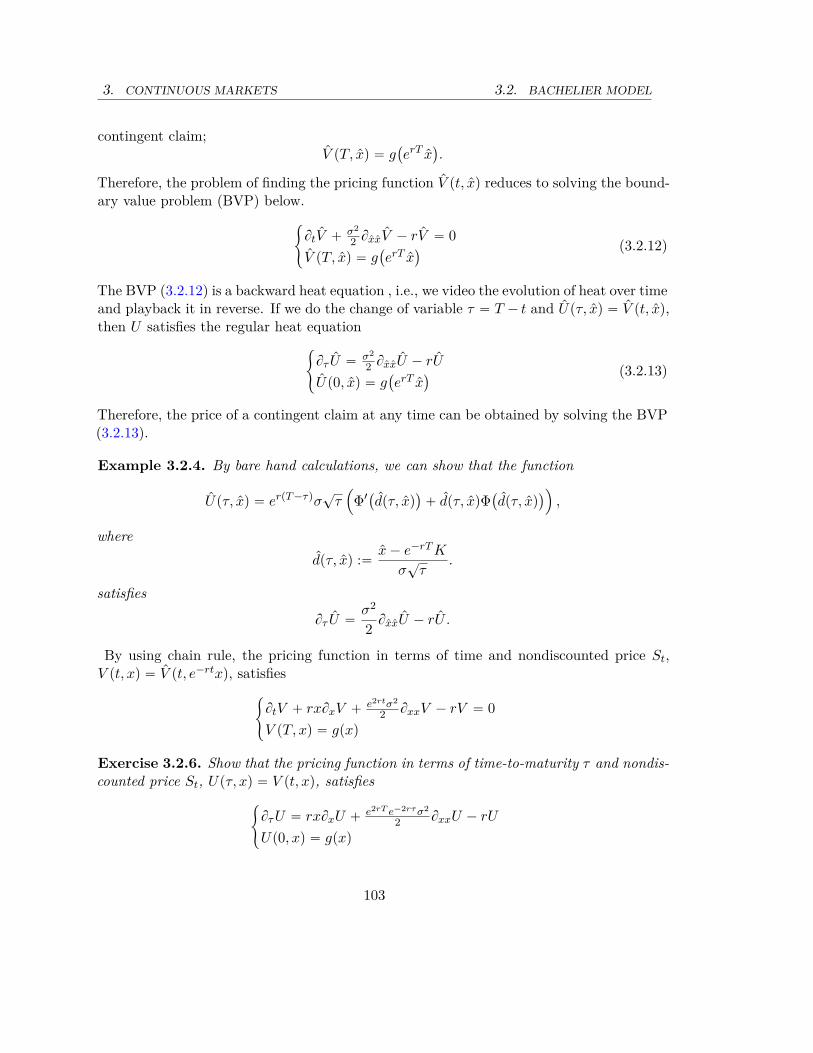
3. CONTINUOUS MARKETS 3.2. BACHELIER MODEL
contingent claim;V pT, xq “ g
`
erT x˘
.
Therefore, the problem of finding the pricing function V pt, xq reduces to solving the bound-ary value problem (BVP) below.
#
BtV ` σ2
2 BxxV ´ rV “ 0V pT, xq “ g
`
erT x˘ (3.2.12)
The BVP (3.2.12) is a backward heat equation , i.e., we video the evolution of heat over timeand playback it in reverse. If we do the change of variable τ “ T ´ t and Upτ, xq “ V pt, xq,then U satisfies the regular heat equation
#
Bτ U “ σ2
2 BxxU ´ rU
Up0, xq “ g`
erT x˘ (3.2.13)
Therefore, the price of a contingent claim at any time can be obtained by solving the BVP(3.2.13).
Example 3.2.4. By bare hand calculations, we can show that the function
Upτ, xq “ erpT ´τqσ?
τ´
Φ1`
dpτ, xq˘
` dpτ, xqΦ`
dpτ, xq˘
¯
,
wheredpτ, xq :“ x ´ e´rT K
σ?
τ.
satisfies
Bτ U “σ2
2BxxU ´ rU .
By using chain rule, the pricing function in terms of time and nondiscounted price St,V pt, xq “ V pt, e´rtxq, satisfies
#
BtV ` rxBxV ` e2rtσ2
2 BxxV ´ rV “ 0V pT, xq “ gpxq
Exercise 3.2.6. Show that the pricing function in terms of time-to-maturity τ and nondis-counted price St, Upτ, xq “ V pt, xq, satisfies
#
Bτ U “ rxBxU ` e2rT e´2rτ σ2
2 BxxU ´ rU
Up0, xq “ gpxq
103
3.2. BACHELIER MODEL 3. CONTINUOUS MARKETS
Exercise 3.2.7. Show that the function
Upτ, xq “ erpT ´τqσ?
τ`
Φ1`
dpτ, xq˘
` dpτ, xqΦ`
dpτ, xq˘˘
,
wheredpτ, xq :“ erpT ´τq x ´ e´rτ K
σ?
τ.
satisfied
BtU “ rxBxU `e2rT e´2rτ σ2
2BxxU ´ rU.
Exercise 3.2.8. Show that the pricing function on nondiscounted price St,
V pt, xq “ V pt, e´rtxq,
satisfies#
BtV ` rxBxV ` e2rtσ2
2 BxxV ´ rV “ 0V pT, xq “ gpxq
Exercise 3.2.9. Show that the discounted pricing function upτ, xq “ e´rτ Upτ, xq satisfiesthe standard form of heat equation below
#
Bτ u “ σ2
2 Bxxu
up0, xq “ gpxq :“ g´
erT x¯ (3.2.14)
Remark 3.2.2 (On regularity of the pricing function). To be able to apply Itô formula in(3.2.11), the pricing function V pt, xq needs to be continuously differentiable on t and twicecontinuously differentiable on x. While the payoff of the option may not be differentiableor value function n continuous, the V pt, xq is regular for all t ă T and all x.
Replication in Bachelier model: Delta Hedging
By (3.1.1), the dynamics of a portfolio in Bachelier model is given by
Wt “ W0 ` r
ż t
0pWs ´ ∆sSsqds `
ż t
0∆sdSs.
Similar to Exercise I.2.1.1, the discounted wealth from portfolio is given by Wt “ e´rtWt
satisfiesWt “ W0 `
ż t
0∆sdSs,
104

3. CONTINUOUS MARKETS 3.2. BACHELIER MODEL
and is a martingale. On the other hand, by applying Itô formula to the discounted optionprice e´rtV pt, Stq, we obtain (3.2.11)
e´rtV pt, Stq “V p0, S0q `
ż t
0e´rs
ˆ
BtV `σ2
2BxxV ´ rV
˙
ps, Ssqds
`
ż t
0e´rsBxV ps, SsqdSs
“V p0, S0q `
ż t
0e´rsBxV ps, SsqdSs.
The last inequality above is by martingale property of discounted option price.
A replicating portfolio is a portfolio such that the terminal wealth WT is equal to thepayoff V pT, ST q “ g
`
erT S˘
. Since both Wt and e´rtV pt, Stq are martingales with WT “
e´rT V pT, ST q “ e´rT g`
erT S˘
, then we must have Wt “ e´rtV pt, Stq for all t P r0, T s.Therefore, V p0, S0q “ W0 and
∆t “ e´rtBxV pt, Stq.
Since ∆t represents the number of units of the underlying in the portfolio, then it followsfrom (3.2.11) that and ∆t is a function of t and St and is given by
∆pt, Stq “ e´rtBxV pt, Stq “ BxV pt, Stq.
Notice that since V is a function of τ “ T ´ t, so is ∆ and
∆pτ, Stq “ e´rtBxV pt, Stq “ e´rpT ´τqBxUpτ, Stq.
To summarize, the issuer of the option must exactly keep ∆t “ e´rtBxV pt, Stq number ofunits of underlying asset at time t in the replicating portfolio. ∆t also accounts for thesensitivity of the option price with respect to the change in the price of underlying.
Example 3.2.5. The replicating portfolio for a call option in Bachelier model is obtainedby taking partial derivative Bx of the function
V callpt, xq “ U callpτ, xq “ erpT ´τqσ?
τ`
Φ1`
dpτ, Stq˘
` dpτ, StqΦ`
dpτ, Stq˘˘
,
withdpτ, xq :“ e´rpT ´τq x ´ e´rτ K
σ?
τ.
105

3.2. BACHELIER MODEL 3. CONTINUOUS MARKETS
Since Bxdpτ, xq “ e´rpT ´τq
σ?
τ, we have
∆pτ, xq “ BxU callpτ, xq
“ e´rpT ´τqσ?
τ´
Bxdpτ, xqΦ2`
dpτ, xq˘
` Bxdpτ, xqΦ`
dpτ, xq˘
` dpτ, xqBxdpτ, xqΦ1`
dpτ, xq˘
¯
“ Φ2`
dpτ, xq˘
` Φ`
dpτ, xq˘
` dpτ, xqΦ1`
dpτ, xq˘
“ Φ`
dpτ, xq˘
.
(3.2.15)
Here Φ1pxq “ 1?2π
e´ x22 is the pdf of standard normal and we used Φ2pxq “ ´x?
2πe´ x2
2 “
´xΦ1pxq.
Example 3.2.6. To find the Bachelier price of an option with payoff gpxq “ ex, we needto solve equation the following BVP for the pricing function.
#
Bτ U “ σ2
2 BxxU ´ rU
Up0, xq “ exp`
erT x˘ .
A possible solution for this problem is Upτ, xq “ eλτ exp`
erT x¯
. If we check this solutionby plugging it in the equation, we obtain
ˆ
λ ´ e2rT σ2
2` r
˙
Upτ, xq “ 0.
Thus, for λ “ e2rT σ2
2 ´r, Upτ, xq satisfies the equation and the initial condition. The Delta-hedging is obtain by ∆pτ, xq “ e´rT erτ BxUpτ, xq “ epλ`rqτ exp
`
erT x˘
“ exp´
e2rT σ2
2 τ¯
exp´
erT x¯
Exercise 3.2.10. Find a closed form solution for the Bachelier price of an option withpayoff gpxq “ 2 cosp
?2xq ´ 3 sinp´xq. Hint: Search for the solution of the form Upτ, xq “
α1eλ1τ cosp?
2xq ` α2eλ2τ sinp´xq.
Example 3.2.7. Let S0 “ $10, σ “ .03, r “ 0.03. The Bachelier Delta of the followingportfolio of vanilla options given in the table below is the linear combination of the Daltas,i.e., 3∆callpτ “ .5, K “ 10q ´ 3∆putpτ “ 1, K “ 10q ´ ∆callpτ “ 2, K “ 8q.
position units type strike maturitylong 3 call $8 .5short 3 put $10 1short 1 call $8 2
The maturities are given in year. Then, (3.2.15) for Delta of call option in Example 3.2.5
106
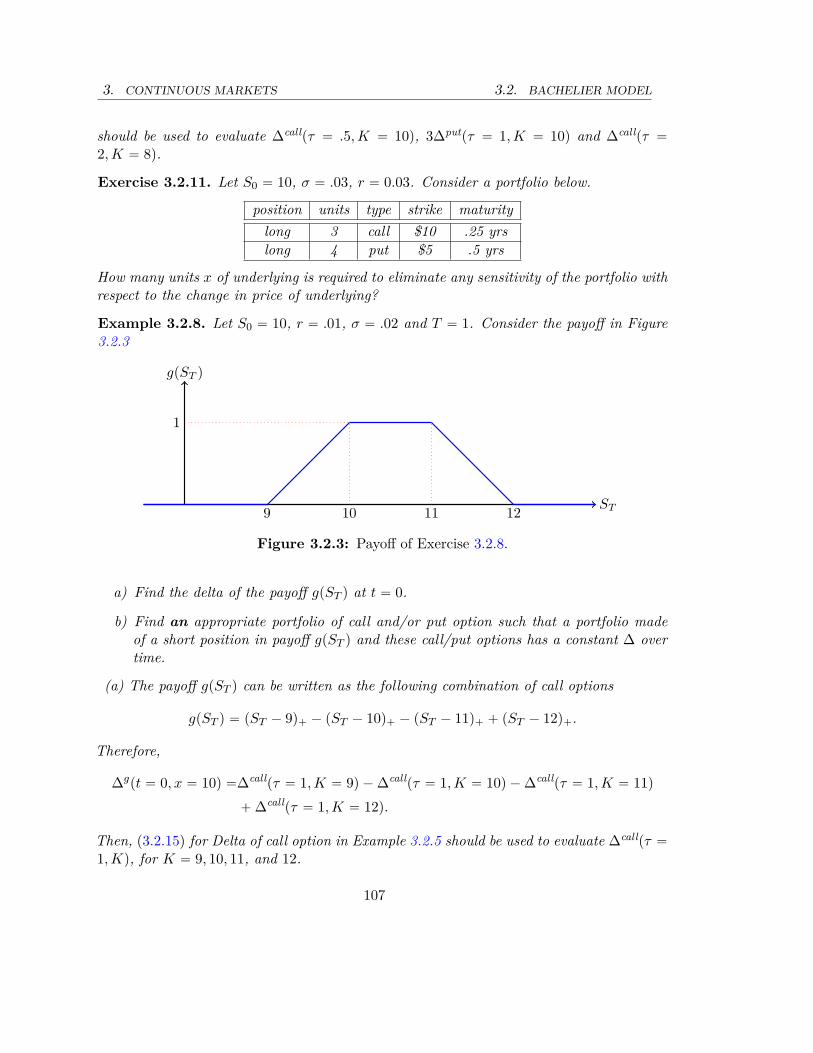
3. CONTINUOUS MARKETS 3.2. BACHELIER MODEL
should be used to evaluate ∆callpτ “ .5, K “ 10q, 3∆putpτ “ 1, K “ 10q and ∆callpτ “
2, K “ 8q.
Exercise 3.2.11. Let S0 “ 10, σ “ .03, r “ 0.03. Consider a portfolio below.
position units type strike maturitylong 3 call $10 .25 yrslong 4 put $5 .5 yrs
How many units x of underlying is required to eliminate any sensitivity of the portfolio withrespect to the change in price of underlying?
Example 3.2.8. Let S0 “ 10, r “ .01, σ “ .02 and T “ 1. Consider the payoff in Figure3.2.3
1
9 10 11 12ST
g(ST )
Figure 3.2.3: Payoff of Exercise 3.2.8.
a) Find the delta of the payoff gpST q at t “ 0.
b) Find an appropriate portfolio of call and/or put option such that a portfolio madeof a short position in payoff gpST q and these call/put options has a constant ∆ overtime.
(a) The payoff gpST q can be written as the following combination of call options
gpST q “ pST ´ 9q` ´ pST ´ 10q` ´ pST ´ 11q` ` pST ´ 12q`.
Therefore,
∆gpt “ 0, x “ 10q “∆callpτ “ 1, K “ 9q ´ ∆callpτ “ 1, K “ 10q ´ ∆callpτ “ 1, K “ 11q
` ∆callpτ “ 1, K “ 12q.
Then, (3.2.15) for Delta of call option in Example 3.2.5 should be used to evaluate ∆callpτ “
1, Kq, for K “ 9, 10, 11, and 12.
107
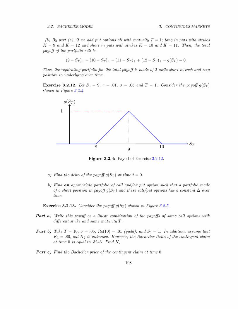
3.2. BACHELIER MODEL 3. CONTINUOUS MARKETS
(b) By part (a), if we add put options all with maturity T “ 1; long in puts with strikesK “ 9 and K “ 12 and short in puts with strikes K “ 10 and K “ 11. Then, the totalpayoff of the portfolio will be
p9 ´ ST q` ´ p10 ´ ST q` ´ p11 ´ ST q` ` p12 ´ ST q` ´ gpST q “ 0.
Thus, the replicating portfolio for the total payoff is made of 2 units short in cash and zeroposition in underlying over time.
Exercise 3.2.12. Let S0 “ 9, r “ .01, σ “ .05 and T “ 1. Consider the payoff gpST q
shown in Figure 3.2.4.
8 109
1
ST
g(ST )
Figure 3.2.4: Payoff of Exercise 3.2.12.
a) Find the delta of the payoff gpST q at time t “ 0.
b) Find an appropriate portfolio of call and/or put option such that a portfolio madeof a short position in payoff gpST q and these call/put options has a constant ∆ overtime.
Exercise 3.2.13. Consider the payoff gpST q shown in Figure 3.2.5.
Part a) Write this payoff as a linear combination of the payoffs of some call options withdifferent strike and same maturity T .
Part b) Take T “ 10, σ “ .05, R0p10q “ .01 (yield), and S0 “ 1. In addition, assume thatK1 “ .80, but K2 is unknown. However, the Bachelier Delta of the contingent claimat time 0 is equal to .3243. Find K2.
Part c) Find the Bachelier price of the contingent claim at time 0.
108
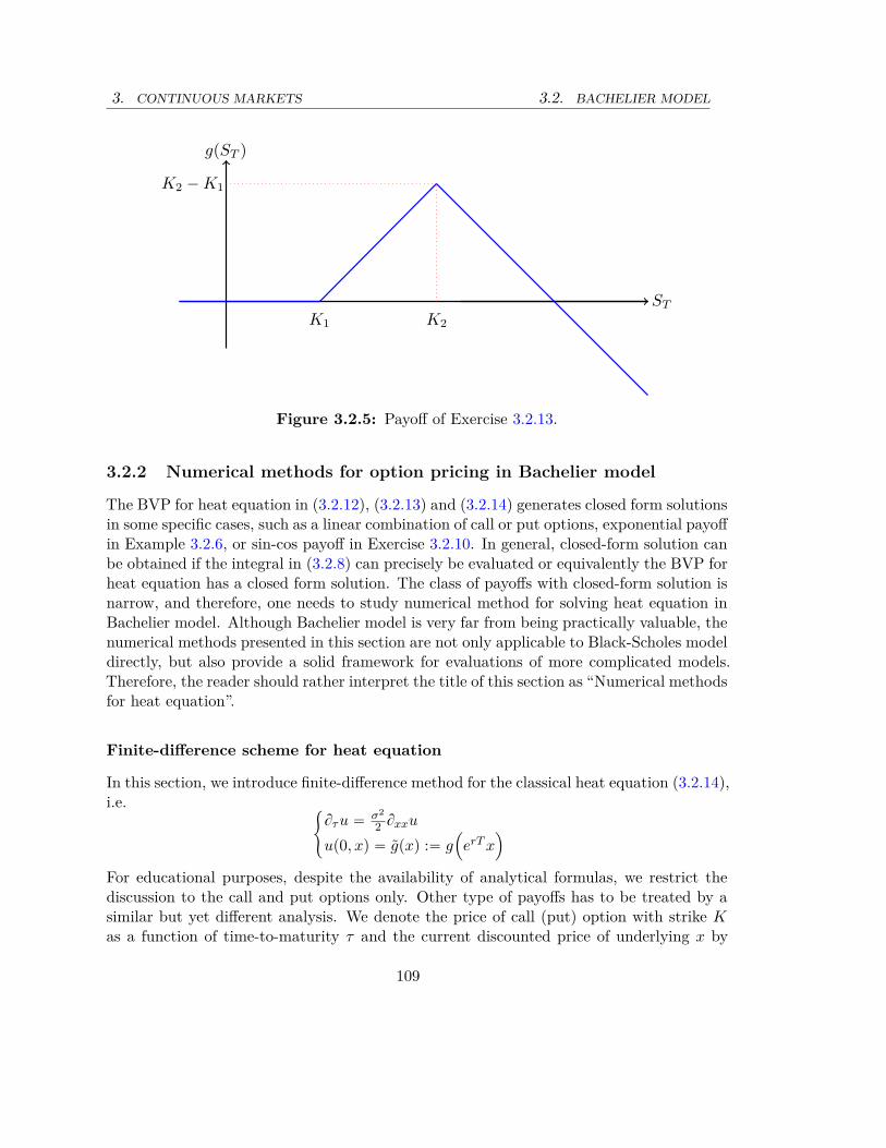
3. CONTINUOUS MARKETS 3.2. BACHELIER MODEL
K1 K2
K2 −K1
ST
g(ST )
Figure 3.2.5: Payoff of Exercise 3.2.13.
3.2.2 Numerical methods for option pricing in Bachelier model
The BVP for heat equation in (3.2.12), (3.2.13) and (3.2.14) generates closed form solutionsin some specific cases, such as a linear combination of call or put options, exponential payoffin Example 3.2.6, or sin-cos payoff in Exercise 3.2.10. In general, closed-form solution canbe obtained if the integral in (3.2.8) can precisely be evaluated or equivalently the BVP forheat equation has a closed form solution. The class of payoffs with closed-form solution isnarrow, and therefore, one needs to study numerical method for solving heat equation inBachelier model. Although Bachelier model is very far from being practically valuable, thenumerical methods presented in this section are not only applicable to Black-Scholes modeldirectly, but also provide a solid framework for evaluations of more complicated models.Therefore, the reader should rather interpret the title of this section as “Numerical methodsfor heat equation”.
Finite-difference scheme for heat equation
In this section, we introduce finite-difference method for the classical heat equation (3.2.14),i.e.
#
Bτ u “ σ2
2 Bxxu
up0, xq “ gpxq :“ g´
erT x¯
For educational purposes, despite the availability of analytical formulas, we restrict thediscussion to the call and put options only. Other type of payoffs has to be treated by asimilar but yet different analysis. We denote the price of call (put) option with strike Kas a function of time-to-maturity τ and the current discounted price of underlying x by
109
3.2. BACHELIER MODEL 3. CONTINUOUS MARKETS
upτ, xq “ Cpτ, xq (upτ, xq “ P pτ, xq), which is the solution of the heat equation (3.2.13)with initial condition up0, xq “
`
erT x ´ K˘
`(up0, xq “
`
K ´ erT x˘
`). One last piece of
setting, we set S0 “ 0 by considering the change of variable Xt “ St ´ S0, i.e., the shiftedprice equal to the difference between the discounted price St and initial price S0.
As the actual domain of heat equation is infinite, in order to apply finite-difference scheme,first we need to choose a finite computational domain, i.e., pτ, xq P r0, T sˆr´xmax, xmaxs fora suitable choice of xmax ą 0. Now since the computational domain is bounded, it inducesmore boundary conditions to the problem at the boundaries x “ xmax and x “ ´xmax.Recall to solve a BVP analytically or numerically, the boundary condition is necessaryat all the boundaries. We should find appropriate boundary conditions at both pointsxmax and ´xmax, which usually relies on the terminal payoff of the option. This type ofboundary conditions which are induced by the computational domain and does not existin the original problem are called artificial boundary conditions, or shortly ABC.
To learn how to set the ABC, let’s study the case for a call option with payoff gpxq “`
erT x´pK `erT S0q˘
`, i.e., up0, xq “ perT x´pK `erT S0qq`. The idea is simply as follows.If x is a very small negative number, then up0, xq “ 0. If the current discounted price of theunderlying is a sufficiently small negative number, the chance that the price at maturityenters the in-the-money region rpK ` erT S0q, 8q is significantly small. For instance, sincethe shifted price Xt “ σBt is a Gaussian random variable, for A ą 0 the probability thatXt ě A (or equivalently Xt ď ´A) is given by
1σ
?2τπ
ż 8
Ae´
y2
2τσ2 dy „12
e´ A22τσ2 , as A Ñ 8,
which is smaller than .006 for A ą 3σ?
T . In other words, far out-of-money options shouldalmost have zero price. On the other hand, when Xt “ x is sufficiently large, the chancethat the discounted price of underlying drops below K ` erT S0 at the maturity T (out-of-money), is significantly small and therefore perT ST ´ Kq` « erT ST ´ K. Far in-the-moneyoptions should almost have almost the same price as the price of payoff ST ´ K, i.e., oneunit of asset minus K units of cash.
For a more rigorous discussion, we actually need the following estimation:
1σ
?2τπ
ż 8
Aye´
y2
2τσ2 dy „σ
?τ
?2π
e´ A22τσ2 , as A Ñ 8.
110
3. CONTINUOUS MARKETS 3.2. BACHELIER MODEL
If we set A :“ e´rT K ` S0 ` e´rT xmax, for xmax sufficiently large we have
upτ, ´xmaxq “e´rτ
σ?
2τπ
ż 8
´8
perT y ´ pK ` erT S0qq`e´py`xmaxq2
2τσ2 dy
“e´rτ
σ?
2τπ
ż 8
e´rT K`S0
perT y ´ pK ` erT S0qqe´py`xmaxq2
2τσ2 dy
“erpT ´τq
σ?
2τπ
ż 8
Apy ´ Aqe´
y2
2τσ2 dy
ďerpT ´τq
σ?
2τπ
ż 8
Aye´
y2
2τσ2 dy „erpT ´τqσ
?τ
?2π
e´ A22τσ2 , as A Ñ 8.
In other words, far out-of-money options should have zero price. This suggests to setupτ, ´xmaxq « 0 for xmax sufficiently large.
On the other hand, if we set B :“ e´rT K ` S0 ´ e´rT xmax
upτ, xmaxq “e´rτ
σ?
2τπ
ż 8
´8
perT y ´ pK ` erT S0qq`e´py´xmaxq2
2τσ2 dy
“erpT ´τq
σ?
2τπ
ż 8
Bpy ´ Bqe´
y2
2τσ2 dy.
Notice that since
1σ
?2τπ
ż 8
Bye´
y2
2τσ2 dy “1
σ?
2τπ
ż B
´8
ye´y2
2τσ2 dy „σ
?τ
?2π
e´ B22τσ2 ,
and1
σ?
2τπ
ż 8
Be´
y2
2τσ2 dy „ 1
as B Ñ ´8, we have
upτ, xmaxq „ ´erpT ´τqB “ e´rτ pxmax ´ pK ` erT S0qq.
Following this observation, we choose ABC for (3.2.16) for the call option is given by
upτ, xmaxq “ e´rτ perT xmax ´ pK ` erT S0qq and upτ, ´xmaxq “ 0.
For put option, put-call parity Proposition 1.2.3 implies that the ABC is given by upτ, xmaxq “
0 and upτ, ´xmaxq “ e´rτ ppK ` erT S0q ´ erT xmaxq.
111
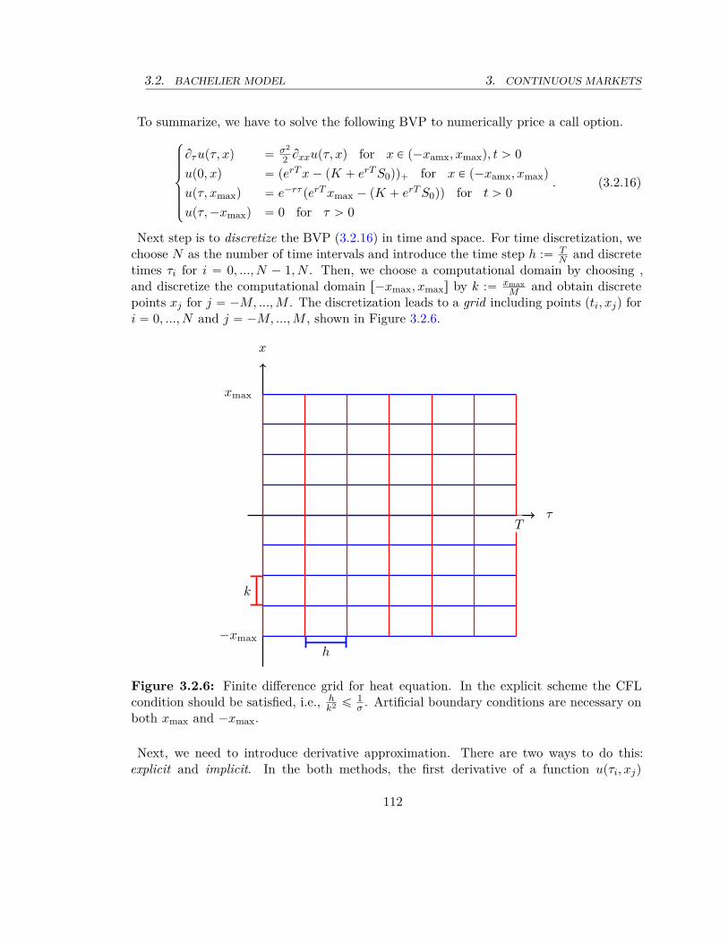
3.2. BACHELIER MODEL 3. CONTINUOUS MARKETS
To summarize, we have to solve the following BVP to numerically price a call option.$
’
’
’
’
&
’
’
’
’
%
Bτ upτ, xq “ σ2
2 Bxxupτ, xq for x P p´xamx, xmaxq, t ą 0up0, xq “ perT x ´ pK ` erT S0qq` for x P p´xamx, xmaxq
upτ, xmaxq “ e´rτ perT xmax ´ pK ` erT S0qq for t ą 0upτ, ´xmaxq “ 0 for τ ą 0
. (3.2.16)
Next step is to discretize the BVP (3.2.16) in time and space. For time discretization, wechoose N as the number of time intervals and introduce the time step h :“ T
N and discretetimes τi for i “ 0, ..., N ´ 1, N . Then, we choose a computational domain by choosing ,and discretize the computational domain r´xmax, xmaxs by k :“ xmax
M and obtain discretepoints xj for j “ ´M, ..., M . The discretization leads to a grid including points pti, xjq fori “ 0, ..., N and j “ ´M, ..., M , shown in Figure 3.2.6.
xmax
−xmax
x
τT
k
h
Figure 3.2.6: Finite difference grid for heat equation. In the explicit scheme the CFLcondition should be satisfied, i.e., h
k2 ď 1σ . Artificial boundary conditions are necessary on
both xmax and ´xmax.
Next, we need to introduce derivative approximation. There are two ways to do this:explicit and implicit. In the both methods, the first derivative of a function upτi, xjq
112

3. CONTINUOUS MARKETS 3.2. BACHELIER MODEL
with respect to time τ at any discrete time τi, i “ 1, ..., N , and any discrete point xj ,j “ ´M ` 1, ..., M ´ 1, is approximated by
Btupτi, xjq «upτi`1, xjq ´ upτi, xjq
h
Then, the second derivative with respect to x can be approximated by
Bxxupτi, xjq «upτi, xj`1q ` upτi, xj´1q ´ 2upτi, xjq
k2 .
Now, we have all the ingredients to present the explicit scheme for heat equation. Thescheme is simply obtained from the heat equation (3.3.24) by simply plugging the aboveapproximations for derivatives, i.e.
upτi`1, xjq ´ upτi, xjq
h“
σ2
2¨
upτi, xj`1q ` upτi, xj´1q ´ 2upτi, xjq
k2 .
τi τi+1
xj+1
xj
xj−1
x
t
Figure 3.2.7: Possible active points in the finite-difference scheme to evaluate upτi`1, xjq,marked with a square. The function u is unknown at dark nodes and known at light nodes.All six nodes are active for implicit scheme with θ‰1. For explicit scheme, θ “ 1, onlyfilled-in nodes are active.
We can simplify the scheme by writing
upτi`1, xjq “
ˆ
1 ´hσ2
k2
˙
upτi, xjq `hσ2
2k2 pupτi, xj`1q ` upτi, xj´1qq . (3.2.17)
113
3.2. BACHELIER MODEL 3. CONTINUOUS MARKETS
In order to use explicit finite-difference scheme in (3.2.17), we need to have the CFL2
conditionh
k2 ď1σ2 .
Otherwise, the scheme does not converges. The right-hand side of CFL condition is always12 times the inverse of the coefficient of second derivative in the equation. For implicitschemes, this condition can be relaxed.Notice that in problem (3.2.16), at τ0 “ 0, the initial condition is known. Therefore, we
setup0, xjq :“ e´rT gperT xjq for j “ ´M, ..., M.
Then, if upτi, xjq is known for all j “ ´M, ..., M , the explicit scheme (3.2.17) suggests thatupτj`1, xjq can be found for all j “ ´M ` 1, ..., M ´ 1. For j “ ´M and M , one can useABC to assign values to upτi, x´M q and upτi, xM q.Implicit scheme is a little more difficult than explicit scheme to implement. But, it has its
own advantages, e.g. the CFL condition is not necessary. To present the implicit methodwe need to modify the approximation of the second derivative as follows.
Bxxupτi, xjq « p1 ´ θqupτi, xj`1q ` upτi, xj´1q ´ 2upτi, xjq
k2
` θupτi`1, xj`1q ` upτi`1, xj´1q ´ 2upτi`1, xjq
k2 .
In the above, θ P r0, 1s is a parameter. If θ “ 0, then the scheme is the same as the explicitscheme. If θ “ 1, we call it a pure implicit scheme. Then for θ ‰ 0, we can present theimplicit scheme as follows.
ˆ
1 ` θhσ2
k2
˙
upτi`1, xjq ´ θhσ2
2k2 pupτi`1, xj`1q ` upτi`1, xj´1qq “
ˆ
1 ´ p1 ´ θqhσ2
k2
˙
upτi, xjq ` p1 ´ θqhσ2
2k2 pupτi, xj`1q ` upτi, xj´1qq .
(3.2.18)
If upτi, xjq is known for all j “ ´M, ..., M , then the right-hand side above is known. Letsdenote the right-hand side by
Rpτi, xjq :“ˆ
1 ´ p1 ´ θqhσ2
k2
˙
upτi, xjq ` p1 ´ θqhσ2
2k2 pupτi, xj`1q ` upτi, xj´1qq .
For j “ M ´ 1, upτi`1, xj`1q on the left-hand side in known. Thus, we move this term to
2Courant-Friedrichs-Lewy
114

3. CONTINUOUS MARKETS 3.2. BACHELIER MODEL
the other sideˆ
1 ` θhσ2
k2
˙
upτi`1, xM´1q ´ θhσ2
2k2 upτi`1, xM´2q “
Rpτi, xM´1q ` θhσ2
2k2 upτi`1, xM q.
Similarly for j “ ´M ` 1 we haveˆ
1 ` θhσ2
k2
˙
upτi`1, x´M`1q ´ θhσ2
2k2 upτi`1, x´M`2q “
Rpτi, x´M`1q ` θhσ2
2k2 upτi`1, x´M q.
To find upτi`1, xjq, one needs to solve the following tridiagonal equation for upτi`1, xjq,j “ ´M ` 1, ..., M ´ 1.
AUi`1 “ Ri ´ Yi (3.2.19)
where A is a 2M ´ 1-by-2M ´ 1 matrix given by
A :“
»
—
—
—
—
—
—
—
—
—
—
–
1 ` θ hσ2
k2 ´θ hσ2
2k2 0 0 ¨ ¨ ¨ 0´θ hσ2
2k2 1 ` θ hσ2
k2 ´θ hσ2
2k2 0 ¨ ¨ ¨ 00 ´θ hσ2
2k2 1 ` θ hσ2
k2 ´θ hσ2
2k2 ¨ ¨ ¨ 0... . . . ...0 ¨ ¨ ¨ ´θ hσ2
2k2 1 ` θ hσ2
k2 ´θ hσ2
2k2 00 ¨ ¨ ¨ 0 ´θ hσ2
2k2 1 ` θ hσ2
k2 ´θ hσ2
2k2
0 ¨ ¨ ¨ 0 0 ´θ hσ2
2k2 1 ` θ hσ2
k2
fi
ffi
ffi
ffi
ffi
ffi
ffi
ffi
ffi
ffi
ffi
fl
,
Yi is a column 2M ´ 1-vector
Yi :“ θhσ2
2k2 pupτi`1, x´M q, 0, ¨ ¨ ¨ , 0, upτi`1, xM qqT,
Ri is a column 2M ´ 1-vector
Ri :“ pRpτi, x´M`1q, ¨ ¨ ¨ , Rpτi, xM´1qqT,
and the unknown column 2M ´ 1-vector
Ui`1 :“ pupτi`1, x´M`1q, ¨ ¨ ¨ , upτi`1, xM´1qqT.
115
3.2. BACHELIER MODEL 3. CONTINUOUS MARKETS
Notice that at the endpoints upτi`1, x´M q and upτi`1, xM q are given by the ABC:
upτi`1, xM q “ e´rτ perT xM ´ pK ` erT S0qq and upt, x´M q “ 0.
The CFL condition for implicit scheme with θ P r0, 1q is given by
h
k2 ď1
p1 ´ θqσ2 .
For the pure implicit scheme (θ “ 1), no condition is necessary for convergence.
Monte Carlo approximation for Bachelier model
The fundamental of the Monte Carlo method is to generate samples based on the underlyingprobability distribution; in the Bachelier model Gaussian distribution with mean S0 andvariance σ2T . The pricing formula
Upτ, xq “ e´rτ ErgperT Sτ q | S0 “ xs.
Given S0 “ x, the random variable Sτ is N px, σ2τq. If txj : j “ 1, ..., Nu are i.i.d. samplesof N p0, 1q, then the expectation ErgperT Sτ q | S0 “ xs can be approximated by
1N
Nÿ
j“1gperT px ` σ
?τxiqq.
Hence, the price of the option Upτ, t, xq can be approximated by
Uapproxpτ, xq “e´rpT ´tq
N
Nÿ
j“1gperT px ` σ
?τxiqq. (3.2.20)
The larger the number of samples N is, the more accurate the approximation Uapproxpτ, xq isobtained. Plain Monte Carlo method is not as efficient as the finite-difference, at least wherethere is only one single risky asset. However, some methods such as variance reduction canbe used to increase its performance.
Quadrature approximation for Bachelier model
Quadrature methods are based on a deterministic (nonrandom) approximation of the inte-gral. In the Bachelier model the price of the option is given by
Upτ, xq “e´rτ
σ?
2πτ
ż 8
´8
g`
erT y˘
e´py´xq2
2σ2τ dy.
116

3. CONTINUOUS MARKETS 3.2. BACHELIER MODEL
As an example of quadrature method, one can first approximate the improper integralabove by the proper integral
e´rτ
σ?
2πτ
ż x`A
x´Ag`
erT y˘
e´py´xq2
2σ2τ dy
and then use Riemann sums to approximate the price of option by
Uapproxpτ, xq “e´rτ
σ?
2πτ
N´1ÿ
j“0g`
erT y˚j
˘
e´py˚
j´xq2
2σ2τ pyj`1 ´ yjq,
where y0 “ x ´ A ă y1 ă ¨ ¨ ¨ ă yN “ x ` A. If the discrete points yj for j “ 0, ..., N arecarefully choses, the quadrature method outperforms plain Monte Carlo method.
Exercise 3.2.14 (Project). Consider the initial price S0, σ, r and payoff assigned to yourgroup.
Group 1 T S0 r σ
1 1 10 .2 12 10 100 .1 53 1 2 .2 .54 2 2 .5 .55 2 2 .5 .56 1 .5 .1 .001
Step 1. Choose a computational domain around the initial price, rS0 ´ xmax, S0 ` xmaxs.
Step 2. Set appropriate artificial boundary conditions (ABC) at the boundary points S0´xmaxand S0 ` xmax.
Step 3. Write a program which implement the implicit finite difference code. The time andspace discretization parameters ph, kq must be set to satisfy
h
k2 ď1
p1 ´ θqσ2 .
Step 4. To make sure your code is correct, run the program for call (or put) option andcompare it for the closed form solution (3.2.9).
Step 5. Run the program for θ “ 0 (explicit), θ “ 12 (semi-implicit) and θ “ 1 (implicit) and
record the result.
Step 6. Simulate a discrete sample path of the price of the underlying asset with the sametime discretization parameter h. By the following algorithm:
117

3.2. BACHELIER MODEL 3. CONTINUOUS MARKETS
Simulating a sample paths of underlying in Bachelier model1: Discretize time by t0 “ 0, ti “ ih, T “ hN .2: for each j “ 1, ..., N do3: Generate a random number wj from standard normal distribution Np0, 1q to represent
pBtj ´ Bjq?
h
4: sj “ sj´1 ` σ?
hwj
5: sj “ ertj sj
6: end forOutput: vector ps0 “ S0, st1 , ..., stN´1 , sT q is a discretely generated sample paths ofBachelier model.
Step 7. Recall that the hedging is given by the derivative BxV pt, Stq “ ertBxV pt, ertStq. Eval-uate the hedging strategy discretely at each node of the discretely generated samplepaths ps0 “ S0, st1 , ..., stN´1q in Step 7, i.e.,
pBxV p0, erts0q, BxV pt1, ert1st1q, ..., ertN´1BxV ptN´1, ertN´1stN´1qq.
Notice that some interpolation may be needed in this step.
Please submit the following outputs:
Output 1. The Program
Output 2. Comparing with the closed form solution for call at p0, S0q.
Output 3. Price and hedging strategy at the points of discrete grid.
3.2.3 Discussion: drawbacks of Bachelier model
One of the drawbacks of the Bachelier model is the possibility of negative realization forasset price. However, this is not the main concern, as in many other application, Gaussianrandom variables are used to model positive quantities such as human weight. Negativeasset price can be problematic if the ratio S0
σ?
Tis not sufficiently large. For instance if the
ratio S0σ
?T
“ 1, then the chance of negative price at maturity T is significant, i.e., higherthat .3.The main concern about Bachelier model is the mismatch with the empirical studies on
the asset return. The return of an asset in Bachelier model is given by
Rartht :“ erpt`δqSt`δ ´ ertSt
ertSt
“erδBt`δ ´ Bt
Bt“
erδpBt`δ ´ Btq
Bt` erδ ´ 1.
118

3. CONTINUOUS MARKETS 3.2. BACHELIER MODEL
10
5 15
-5
ST
g(ST )
Group 140
80 100
-40
140ST
g(ST )
Group 2
1 32
1
ST
g(ST )
Group 3
1 32
1
ST
g(ST )
Group 4
1 32
1
ST
g(ST )
Group 5
.25
.75
-.25
.75
.5.25ST
g(ST )
Group 6
Figure 3.2.8: Differenet payoff for the project
Formally, since Bt`δ ´ Bt and Bt are independent, we have
ErRartht s “ erδ ErBt`δ ´ Bts
looooooomooooooon
“0
E„
1Bt
ȷ
` erδ ´ 1 “ erδ ´ 1 « rδ.
119

3.3. CONTINUOUS-TIME MARKET OF BLACK-SCHOLES3. CONTINUOUS MARKETS
However, the above formal calculation is faulty. The random variable 1Bt
is not integrable;
E„
1|Bt|
ȷ
“1
?2tπ
ż
R
1|x|
e´ x22t dx “ 8.
3.3 Continuous-time market of Black-Scholes
Black-Scholes model can be obtained by asymptotic methods from the binomial model. Todo this, we first present some asymptotic properties of binomial model.
3.3.1 Black-Scholes model: limit of binomial under risk-neutral proba-bility
Let T ą 0 be a real number and N be a positive integer. We divide T units of time intoN time intervals, each of size δ :“ T
N3. Then, consider a binomial model with N periods
given by the times t0 “ 0 ă t1 “ δ, ..., tk “ kδ, ...tN “ T . Recall from binomial model that
Spk`1qδ “ SkδHk`1, for k “ 0, ..., N ´ 1
where, in accordance to the Assumption 2.3.1, the random variables tHkuNk“1 is a sequence
of i.i.d. random variables with the following distribution
Hk “
#
u with probability π
ℓ with probability 1 ´ π
Asymptotics of parameters u, ℓ, and p
The goal of this section is to show the following approximations:
u “ 1 ` δr `?
δσα “ eδpr´ σ22 q`
?δσα ` opδq,
ℓ “ 1 ` δr ´?
δσβ “ eδpr´ σ22 q´
?δσβ ` opδq.
(3.3.1)
To obtain this approximation, one should notice that from (2.3.5), we have x0 “ 1 ` λ?
δ2 `
op?
δq. Thus, it follows from (2.3.4) that
1 ´ p
p“ x2
0 “ 1 ` λ?
δ ` op?
δq and p “12
´λ
?δ
4` op
?δq.
3Each time unit is divided into 1δ small time intervals.
120

3. CONTINUOUS MARKETS 3.3. BLACK-SCHOLES MODEL
Then,
α2 “1 ´ p
p` 2λ
?δ
c
1 ´ p
p` op
?δq “ x2
0 “ 1 ` 3λ?
δ ` op?
δq. (3.3.2)
On the other hand, one can easily see that4
eδpr´ σ22 q`
?δσα “ 1 ` δpr ´
σ2
2q `
?δσα `
pδpr ´ σ2
2 q `?
δσαq2
2` opδq
“ 1 ` δpr ´σ2
2q `
?δσα `
δσ2α2
2` opδq
“ 1 ` δr `?
δσα `δpσ2 ´ 1qα2
2` opδq
“ 1 ` δr `?
δσα ` opδq.
In the above we used (3.3.2), i.e., σ2 ´ 1 “ Op?
δq.
Similarly, we have β2 “ 1 ´ 3λ?
δ ` op?
δq and
eδpr´ σ22 q´
?δσβ “ 1 ` δr ´
?δσβ ` opδq.
Arithmetic return versus log return
This asymptotics yields to the relation between the arithmetic return and log return inbinomial model. While the arithmetic return is given by
Rartht “
#
δr `?
δσα
δr ´?
δσβ
the log return is given by
Rlogt “
#
δpr ´ σ2
2 q `?
δσα ` opδq
δpr ´ σ2
2 q ´?
δσβ ` opδq.
The probabilities of the values in both returns are given by pπ, 1 ´ πq for risk-neutralprobability and pp, 1 ´ pq for physical probability. In particular, if E and E are respectivelyexpectation with respect to risk-neutral probability and physical probability, then we have
4ex “ 1 ` x ` x2
2 ` opx2q
121
3.3. BLACK-SCHOLES MODEL 3. CONTINUOUS MARKETS
ErRartht s “ rδ, and ErpRarth
t q2s “ σ2δ ` opδq
ErRartht s “ µδ, and ErpRarth
t q2s “ σ2δ ` opδq
ErRlogt s “ pr ´
12
σ2qδ, and ErpRlogt q2s “ σ2δ ` opδq
ErRlogt s “ pµ ´
12
σ2qδ, and ErpRlogt q2s “ σ2δ ` opδq.
(3.3.3)
Weak convergence of binomial model to geometric Brownian motion
From the asymptotics in (3.3.3), the log return of calibrated binomial model is given by
Rlogt “ lnpHkq “
#
δpr ´ σ2
2 q `?
δσα with probability π
δpr ´ σ2
2 q ´?
δσβ with probability 1 ´ π
Indeed,lnpSpk`1qδq “ lnpSkδq ` lnpHk`1q,
or
lnpStq “ lnpS0q `
Nÿ
k“1lnpHkq.
Let tZkuNk“1 is a sequence of i.i.d. random variables with the following distribution
Zk “
#
α with probability π
´β with probability 1 ´ π
Then, we have
lnpST q “ lnpS0q ` pr ´σ2
2qT ` σ
?T ¨
1?
N
Nÿ
k“1Zk. (3.3.4)
Next, we want to show that the normalized summation 1?N
řNk“1 Zk converges weakly to
a random variable (distribution) as the number of time intervals N approaches to infinity5.To show this, from Theorem B.9 from the appendix, we only need to find
limNÑ8
χ 1?N
řNk“1 Zk
pθq.
Notice that here the characteristic function is under risk-neutral probability, i.e., χXpθq “
EreiθXs.
5Or equivalently δ Ñ 0.
122

3. CONTINUOUS MARKETS 3.3. BLACK-SCHOLES MODEL
Since tZtuNk“1 is a sequence of i.i.d. random variables, we have
χ 1?N
řNk“1 Zk
pθq “
Nź
k“1χZ1
ˆ
θ?
N
˙
.
On the other hand,
χZ1pθq “ EreiθZ1s “ 1 ` iθErZ1s ´θ2ErZ2
1 s
2` opθ2q.
Notice that by (2.3.2), we can write
π “R ´ L
U ´ L“
β
α ` β. (3.3.5)
Therefore, straightforward calculations show that ErZ1s “ 0, and ErZ21 s “ 1. By using
Taylor expansion of the characteristic function, we obtain
χZ1
ˆ
θ?
N
˙
“ 1 ´θ2
2N` op
1N
q,
and
χ 1?N
řNk“1 Zk
pθq “
ˆ
1 ´θ2
2N` op
1N
q
˙N
,
By sending n Ñ 8, we obtain
limNÑ8
χ 1?N
řNk“1 Zk
pθq “ limNÑ8
ˆ
1 ´θ2
2N` op
1N
q
˙N
“ e´ θ22 .
Since e´ θ22 is the characteristic function of standard normal random variable, we conclude
that 1?N
řNk“1 Zk converges weakly to N p0, 1q.
Exercise 3.3.1. In the above calculations, explain why we cannot apply central limit the-orem (Theorem B.7) directly.
(3.3.4) suggests that we define a continuous-time model for the price St of the asset attime T as the weak limit of the binomial model by
lnpST q “ lnpS0q ` pr ´σ2
2qT ` σN p0, T q
or equivalently
ST “ S0 expˆ
pr ´σ2
2qT ` σN p0, T q
˙
.
123
3.3. BLACK-SCHOLES MODEL 3. CONTINUOUS MARKETS
Calibrating binomial model: revised
In the above, we see that the choice of parameters u, ℓ, and R leads to we made a perfectchoice of ErZ1s “ 0 and ErZ2
1 s “ 1. However, in (3.3.4), the only criteria for the convergenceof binomial model to Black-Scholes model is that the random variables Zk, k “ 1, ..., Nmust satisfy ErZ1s “ opδq and ErZ2
1 s “ 1 ` op1q, i.e.
If ErZ1s “ opδq, and ErZ21 s “ 1`op1q, then 1
?N
Nÿ
k“1Zk convergens to N p0, 1q weakly.
(3.3.6)To avoid the calculation of α and β, one can choose different parameters for the bino-
mial tree. Notice that the binomial model has three parameters u, ℓ and R while theBlack-Scholes parameters are only two. This degree of freedom provides us with somemodifications of binomial three which still converges to the Black-Scholes formula. Thisalso simplifies the calibration process in Section 2.3 significantly simpler. Here are somechoices:
a) Symmetric probability:
u “ eδpr´ σ22 q`
?δσ, ℓ “ eδpr´ σ2
2 q´?
δσ, and R “ rδ,
Then;πu “ πℓ “
12
.
Notice that (3.3.4) should be modified by setting thetZkuNk“1 distribution of i.i.d.
sequence
Z1 “
#
1 with probability 12
´1 with probability 12
and ErZ1s “ 0 and ErZ21 s “ 1.
b) Subjective return:
u “ eδν`?
δσ, ℓ “ eδν´?
δσ, and R “ rδ,
Then;
πu “12
˜
1 `?
δr ´ ν ´ 1
2σ2
σ
¸
and πℓ “12
˜
1 ´?
δr ´ ν ´ 1
2σ2
σ
¸
.
In this case, (3.3.4) should be modified by setting thetZkuNk“1 distribution of i.i.d.
124
3. CONTINUOUS MARKETS 3.3. BLACK-SCHOLES MODEL
sequence
Z1 “
$
&
%
?δ
ν´r` 12 σ2
σ ` 1 with probability πu?
δν´r` 1
2 σ2
σ ´ 1 with probability πℓ
and ErZ1s “ 0 and ErZ21 s “ 1 `
´
ν´r` 12 σ2
σ
¯2δ.
Exercise 3.3.2. Show
ErZ1s “ opδq, and ErZ21 s “ 1 ` op1q.
in the following cases.
a) symmetric probability
b) subjective return
Exercise 3.3.3. Consider risk-neutral trinomial model with N periods presented by
Spk`1qδ “ SkδHk`1, for k “ 0, ..., N ´ 1
where δ :“ TN and tHkuN
k“1 is a sequence of i.i.d. random variables with distribution
Hk “
$
’
’
&
’
’
%
eδpr´ σ22 q`
?3δσ with probability π “ 1
6
eδpr´ σ22 q with probability 1 ´ 2π “ 2
3
eδpr´ σ22 q´
?3δσ with probability π “ 1
6
and π ă 12 . Show that as δ Ñ 0, this trinomial model converges to the black-Scholes model
in the weak sense.Hint: Find Zk such that lnpHkq “ pr ´ σ2
2 qδ ` σ?
δZk. Then, show (3.3.6)
3.3.2 Pricing contingent claims in Black-Scholes model
Recall from the last section that the limit of binomial model under risk-neutral probabilityyields the geometric Brownian motion
St “ S0 expˆ
pr ´σ2
2qt ` σBt
˙
. (3.3.7)
We can use this random variable St to price an option in this continuous setting. We startwith a call option with maturity T and strike price K.Inspired by Arrow-Debreu market model, the price of this call option is the discounted
expected value of pST ´ Kq` under risk-neutral probability. To calculated this price, we
125

3.3. BLACK-SCHOLES MODEL 3. CONTINUOUS MARKETS
only need to know the distribution of St under risk-neutral probability which is given by(3.3.7). Since St is a function of a standard normal random variable, we obtain
ErpST ´ Kq`s “1
?2π
ż 8
´8
ˆ
S0 expˆ
pr ´σ2
2qT ` σ
?Tx
˙
´ K
˙
`
expˆ
´x2
2
˙
dx.
Notice that when x ď x˚ :“ 1σ
?T
´
lnpKS0q ´ pr ´ σ2
2 qT¯
, the the integrand is zero andotherwise pST ´ Kq` “ St ´ K. Therefore,
ErpST ´ Kq`s “ S0epr´ σ22 qT
ż 8
x˚
eσ?
T x´ x22
?2π
dx ´ K
ż 8
x˚
e´ x22
?2π
dx
“ S0erT
ż 8
x˚
e´px´σ
?T q2
2?
2πdx ´ K
ż 8
x˚
e´ x22
?2π
dx
“ S0erT
ż 8
x˚`σ?
T
e´ x22
?2π
dx ´ K
ż 8
x˚
e´ x22
?2π
dx
Notice thatş8
x˚e´ x2
2?
2πdx is the probability that a standard normal random variable is greater
than x˚ andş8
x˚`σ?
Te´ x2
2?
2πdx is the probability that a standard normal random variable is
greater than x˚ ` σ?
T . Simple calculation shows that
x˚ ` σ?
T “1
σ?
T
ˆ
lnpKS0q ´ pr `σ2
2qT
˙
.
In other words, the price of a European call option is given by
CpT, K, S0, 0q :“ e´rT ErpSt ´ Kq`s “ S0Φ pd1q ´ e´rT KΦ pd2q ,
d1 “1
σ?
T
ˆ
lnpS0Kq ` pr `σ2
2qT
˙
and d2 “1
σ?
T
ˆ
lnpS0Kq ` pr ´σ2
2qT
˙
.
(3.3.8)
Here Φpxq “şx
´8e´
y22
?2π
dy is the standard normal distribution function.6
Exercise 3.3.4. Use put-call parity to show Black-Scholes formula for the price of a putoption with maturity T and strike K is given by
P pT, K, S0, 0q :“ e´rT KΦ p´d2q ´ S0Φ p´d1q .
6In the above calculations, we use 1 ´ Φpxq “ Φp´xq.
126
3. CONTINUOUS MARKETS 3.3. BLACK-SCHOLES MODEL
For a general contingent claim, the price of derivative with payoff gpStq in Black-Scholesmodel is given by
V0pS0q :“ e´rT ErgpST qs “ e´rT E„
g
ˆ
epr´ σ22 qT `σ
?T N p0,1q
˙ȷ
“1
?2π
ż 8
´8
g
ˆ
epr´ σ22 qT `σ
?T x
˙
e´ x22 dx.
As a consequence of Assumption 2.3.1, the random variables if we repeat the calculationsin Section 3.3.1, we obtain
St “ S0 expˆ
pr ´σ2
2qt ` σN p0, tq
˙
and ST “ St expˆ
pr ´σ2
2qpT ´ tq ` σN p0, T ´ tq
˙
.
Now we would like to explain the relation between the two normal random variablesN p0, T ´ tq and N p0, tq in the above. Thus, in Black-Scholes model, ST
Stis independent of
St. This, in particular, implies that Black-Scholes model is Markovian7 and the priceof a call option with strike K and maturity T given the price of underlying asset at timet is equal to St is a function of St and t but not Su for u ă t. As a result the price of calloption at time t given St “ S is given by
CpT, K, S, tq :“ e´rpT ´tqErpST ´ Kq` | St “ Ss “ SΦ pd1q ´ e´rpT ´tqKΦ pd2q ,
d1 “1
σ?
T ´ t
ˆ
lnpSKq ` pr `σ2
2qpT ´ tq
˙
and
d2 “1
σ?
T ´ t
ˆ
lnpSKq ` pr ´σ2
2qpT ´ tq
˙
.
In general, Markovian property implies that for a general contingent claim, the price ofderivative with payoff gpStq, the Black-Scholes price at time t is a function V pt, Stq :“e´rpT ´tqErgpST q | Sts. We will study some more properties of this function V : r0, T s ˆ
R` Ñ R in the future. In Black-Scholes market, contingent claims that have payoff isgpST q, a function of underlying price at time T , St, are called Markovian claims and theprice of a Markovian claim is given by
V pt, Sq :“ e´rpT ´tqErgpST q | St “ Ss “ e´rpT ´tqE„
g
ˆ
epr´ σ22 qpT ´tq`σ
?T ´tN p0,1q
˙ȷ
“e´rpT ´tq
?2π
ż 8
´8
g
ˆ
S`
epr´ σ22 qpT ´tq`σ
?T ´tx
˘
˙
e´ x22 dx.
(3.3.9)
7Future movements of the price are independent of the past.
127

3.3. BLACK-SCHOLES MODEL 3. CONTINUOUS MARKETS
Remark 3.3.1. Price of a Markovian claim in Black-Scholes model does not depend onthe past movements of the price and it only depends on the current price St. This isnot true for nonMarovian claims, indeed. For example a look-back option with payoffpmax0ďtďT St ´ Kq` or Asian option
´
1T
şT0 St ´ K
¯
`are nonMarkovian options with the
price which depends to some extent in the past history of the price movement rather thanonly the current price of the underlying.
As seen in (3.3.9), the Black-Scholes price of a Markovian European option is always afunction of T ´ t rather than t and T separately. Therefore, we can introduce the newvariable τ :“ T ´ t which is called time-to-maturity. Then, one can write the value of theMarkovian European option as a function of τ and S by
V pτ, Sq :“ e´rτ ErgpSτ q | S0 “ Ss “e´rτ
?2π
ż 8
´8
g
ˆ
S`
epr´ σ22 qτ`σ
?τx˘
˙
e´ x22 dx.
For call option the Black-Scholes formula in terms of τ is given by
Cpτ, K, Sq “ SΦ pd1q ´ e´rτ KΦ pd2q ,
d1 “1
σ?
τ
ˆ
lnpSKq ` pr `σ2
2qτ
˙
and d2 “1
σ?
τ
ˆ
lnpSKq ` pr ´σ2
2qτ
˙
.(3.3.10)
3.3.3 Delta Hedging
As seen in the binomial model, to hedge the risk of issuing an option, one has to constructa replicating portfolio. The replicating portfolio contains ∆tpStq units of risky asset attime t if the price of the asset is equal to St where by (2.2.4)
∆tpSq :“ Vt`δpSuq ´ Vt`δpSℓq
Spu ´ ℓq.
Using (3.3.1), we have
∆tpSq “Vt`δpS ` Spδr `
?δσαqq ´ Vt`δpS ` Sp1 ` δr ´
?δσβqq
S?
δσpα ` βq
Heuristically, as δ Ñ 0, we obtain the Delta of the Black-Scholes model as
∆BSt pSq “ BSV pt, Sq, (3.3.11)
where V pt, Sq is the Black-Scholes price of a general contingent claim with any given payoff.We can also find another heuristic derivation of this result. In the binomial model, we
128

3. CONTINUOUS MARKETS 3.3. BLACK-SCHOLES MODEL
can write
ErgpST q | St`δ “ Sus “ ErgpST ´δuq | St “ Ss and ErgpST q | St`δ “ Sℓs “ ErgpST ´δlq | St “ Ss.
This is because binomial model is time homogeneous. Therefore,
∆tpSq “Vt`δpSuq ´ Vt`δpSℓq
Spu ´ ℓq
“ e´rpT ´tq ErgpST q | St`δ “ Sus ´ ErgpST q | St`δ “ Sℓs
Spu ´ ℓq` Opδq
“ e´rpT ´tq ErgpST ´δuq | St “ Ss ´ ErgpST ´δlq | St “ Ss
Spu ´ ℓq` Opδq
“ e´rpT ´tq ErST ´δV 1pST ´δq | St “ Sspu ´ ℓq
Spu ´ ℓq` Opδq.
In the above we used (3.3.1) to obtain pu ´ ℓq2 “ Opδq and
V pxq ´ V pyq “ V 1pxqpy ´ xq ` Oppx ´ yq2q.
Hence,
∆tpSq “e´rpT ´tq
SErST ´δV 1pST ´δq | St “ Ss ` Opδq
Now by weak convergence of underlying asset price in binomial model to asset price inBlack-Scholes model, as δ Ñ 0, we obtain
∆BSt pSq “
e´rpT ´tq
SErST V 1pST q | St “ Ss.
Notice that given St “ S we have
ST “ S expˆ
pr ´σ2
2qpT ´ tq ` σN p0, T ´ tq
˙
.
Therefore,
BS
´
gpST q
¯
“ expˆ
pr ´σ2
2qpT ´ tq ` σN p0, T ´ tq
˙
V 1pST q “ST
SV 1pST q.
129
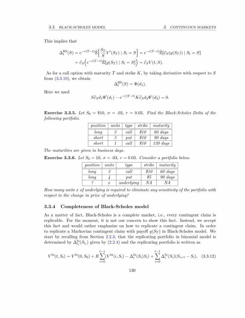
3.3. BLACK-SCHOLES MODEL 3. CONTINUOUS MARKETS
This implies that
∆BSt pSq “ e´rpT ´tqE
”ST
SV 1pST q | St “ S
ı
“ e´rpT ´tqErBSpgpST qq | St “ Ss
“ BS
´
e´rpT ´tqErgpST q | St “ Ss
¯
“ BSV pt, Sq.
As for a call option with maturity T and strike K, by taking derivative with respect to Sfrom (3.3.10), we obtain
∆BSt pSq “ Φpd1q.
Here we usedSBSd1Φ1pd1q ´ e´rpT ´tqKBSd2Φ1pd2q “ 0.
Exercise 3.3.5. Let S0 “ $10, σ “ .03, r “ 0.03. Find the Black-Scholes Delta of thefollowing portfolio.
position units type strike maturitylong 3 call $10 60 daysshort 3 put $10 90 daysshort 1 call $10 120 days
The maturities are given in business days.Exercise 3.3.6. Let S0 “ 10, σ “ .03, r “ 0.03. Consider a portfolio below.
position units type strike maturitylong 3 call $10 60 dayslong 4 put $5 90 days
? x underlying NA NAHow many units x of underlying is required to eliminate any sensitivity of the portfolio withrespect to the change in price of underlying?
3.3.4 Completeness of Black-Scholes model
As a matter of fact, Black-Scholes is a complete market, i.e., every contingent claim isreplicable. For the moment, it is not our concern to show this fact. Instead, we acceptthis fact and would rather emphasize on how to replicate a contingent claim. In orderto replicate a Markovian contingent claim with payoff gpST q in Black-Scholes model. Westart by recalling from Section 2.2.3, that the replicating portfolio in binomial model isdetermined by ∆bi
tipStiq given by (2.2.4) and the replicating portfolio is written as
V bipt, Stq “ V bip0, S0q ` Rt´1ÿ
i“0pV bipi, Siq ´ ∆bi
i pSiqSiq `
t´1ÿ
i“0∆bi
i pSiqpSi`1 ´ Siq, (3.3.12)
130
3. CONTINUOUS MARKETS 3.3. BLACK-SCHOLES MODEL
By taking limit from (3.3.12), we obtain
V pT, Stq “ V p0, S0q ` R
ż T
0pV pt, Stq ´ ∆tpStqStqdt `
ż T
0∆tpStqdSt. (3.3.13)
In the above V pt, Sq is the Black-Scholes price of the contingent claim and ∆tpStq satisfies(3.3.11). The first integral in (3.3.13) is a simple Riemann integral. The second integralis a more complicated stochastic integral, i.e., the integrator dSt is stochastic. We willmake sense of the stochastic integration in the future by defining Itô integral. But for themoment, you can use the heuristics of Riemann-Stieltjes integral for stochastic integral,limit of
řN´1i“0 ∆tipStiqpSti`1 ´ Stiq.
3.3.5 Error of discrete hedging in Black-Scholes model and Greeks
Equation (3.3.13) suggests to adjust Delta continuously in time to replicate the contingentclaim. On one hand, this is a useful formula because in reality trading can happen withenormous speed which makes continuous-time a fine approximation. However, in practice,the time is still in discrete and hedging is only a time lapse. Therefore, it is important tohave some estimation on the error of discrete-time hedging in Black-Scholes framework.
Let us consider that the Black-Scholes model is running continuous in time, but we onlyadjust our position on the approximately replicating portfolio at times ti :“ δi where δ “ T
Nand i “ 0, 1, ..., N . By setting aside the accumulated error until time ti, we can assumethat our hedge has been perfect until time ti, for some i, i.e.
V pti, Stiq “ ∆BSti
pStiqSti ` Yti ,
where V pt, Sq is the Black-Scholes value of the contingent claim, and Yt is the position incash. At time ti`1 “ ti ` δ, the value of the portfolio is
∆BSti
pStiqSti`δ ` erδYti .
131
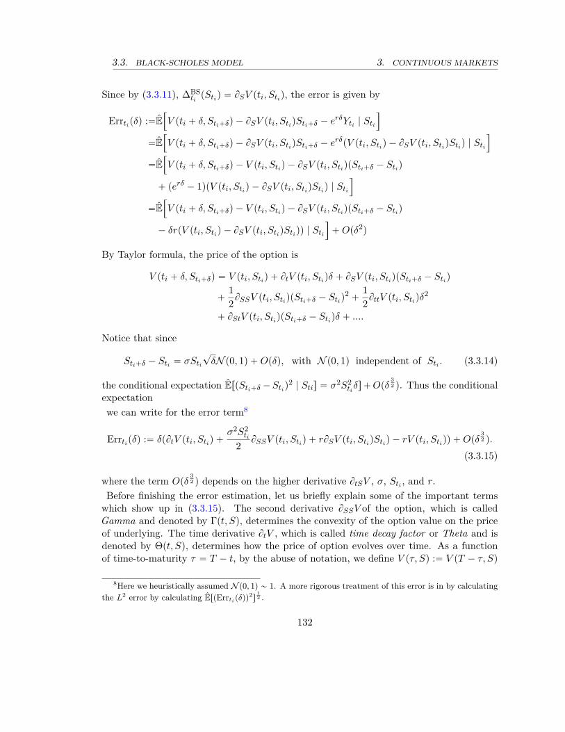
3.3. BLACK-SCHOLES MODEL 3. CONTINUOUS MARKETS
Since by (3.3.11), ∆BSti
pStiq “ BSV pti, Stiq, the error is given by
Errtipδq :“E”
V pti ` δ, Sti`δq ´ BSV pti, StiqSti`δ ´ erδYti | Sti
ı
“E”
V pti ` δ, Sti`δq ´ BSV pti, StiqSti`δ ´ erδpV pti, Stiq ´ BSV pti, StiqStiq | Sti
ı
“E”
V pti ` δ, Sti`δq ´ V pti, Stiq ´ BSV pti, StiqpSti`δ ´ Stiq
` perδ ´ 1qpV pti, Stiq ´ BSV pti, StiqStiq | Sti
ı
“E”
V pti ` δ, Sti`δq ´ V pti, Stiq ´ BSV pti, StiqpSti`δ ´ Stiq
´ δrpV pti, Stiq ´ BSV pti, StiqStiqq | Sti
ı
` Opδ2q
By Taylor formula, the price of the option is
V pti ` δ, Sti`δq “ V pti, Stiq ` BtV pti, Stiqδ ` BSV pti, StiqpSti`δ ´ Stiq
`12
BSSV pti, StiqpSti`δ ´ Stiq2 `
12
BttV pti, Stiqδ2
` BStV pti, StiqpSti`δ ´ Stiqδ ` ....
Notice that since
Sti`δ ´ Sti “ σSti
?δN p0, 1q ` Opδq, with N p0, 1q independent of Sti . (3.3.14)
the conditional expectation ErpSti`δ ´ Stiq2 | Stis “ σ2S2
tiδs ` Opδ
32 q. Thus the conditional
expectationwe can write for the error term8
Errtipδq :“ δpBtV pti, Stiq `σ2S2
ti
2BSSV pti, Stiq ` rBSV pti, StiqStiq ´ rV pti, Stiqq ` Opδ
32 q.
(3.3.15)
where the term Opδ32 q depends on the higher derivative BtSV , σ, Sti , and r.
Before finishing the error estimation, let us briefly explain some of the important termswhich show up in (3.3.15). The second derivative BSSV of the option, which is calledGamma and denoted by Γpt, Sq, determines the convexity of the option value on the priceof underlying. The time derivative BtV , which is called time decay factor or Theta and isdenoted by Θpt, Sq, determines how the price of option evolves over time. As a functionof time-to-maturity τ “ T ´ t, by the abuse of notation, we define V pτ, Sq :“ V pT ´ τ, Sq
8Here we heuristically assumed N p0, 1q „ 1. A more rigorous treatment of this error is in by calculatingthe L2 error by calculating ErpErrti pδqq2s
12 .
132

3. CONTINUOUS MARKETS 3.3. BLACK-SCHOLES MODEL
and therefore, we have
∆pτ, Sq “ BSV pτ, Sq
Γpτ, Sq “ BSSV pτ, Sq
Θpτ, Sq “ ´Bτ V pτ, Sq
For example in the case of call option with strike K and maturity T , by taking derivativesBSS and Bτ in (3.3.10), we have
Γpτ, Sq “1
Sσ?
τΦ1pd1q and Θpτ, Sq “ ´
Sσ
2?
τΦ1pd1q ´ rKe´rτ Φpd2q. (3.3.16)
The ∆, Γ, and Θ of a call option in Black-Scholes model is shown in Figure 3.3.1.
6 8 10 12 14
−0.5
0
0.5
1
S
DeltaGammaTheta
Figure 3.3.1: Greeks of call option with τ “ 1, σ “ .1, r “ .05, and K “ 10. As you seethe significant sensitivity is near the ATM.
To continue with the error estimation, we need the following proposition.Proposition 3.3.1. For a European Markovian contingent claim, the Black-Scholes pricesatisfies
Θpτ, Sq “ ´σ2S2
2Γpτ, Sq ´ rS∆pτ, Sq ` rV pτ, Sq.
As a result of this proposition, the term f order δ in (3.3.15) vanishes and thus one steperror is of order Opδ
32 q. Provided that the term Opδ
32 q remains bounded, we have
Errpδq :“ E
«
N´1ÿ
i“0Errtipδq
ff
“ Op?
δq,
133

3.3. BLACK-SCHOLES MODEL 3. CONTINUOUS MARKETS
which converges to 0 as fast as?
δ when δ Ñ 0.
Discrete hedging without money market account
One reason to completely disregard the money market account is because the risk-freeinterest rate r is not exactly constant. The money market is also under several risks whichis a different topic. To understand this better, let us first consider the issuer of an optionwhich is long in ∆BSpti, Stiq units of underlying. Then the change in the portfolio fromtime ti to time ti ` δ is
ErV pti ` δ, Sti`δq ´ V pti, Stiq ´ ∆BSpti, StiqpSti`δ ´ Stiqs
“ pBtV pti, Stiq `σ2S2
ti
2BSSV pti, Stiqqδ ` opδq,
where we used (3.3.14) in the right-hand side. This error is related to loss/profit of notperfectly hedging and is called slippage error ; see Figure 3.3.2.
Sti Sti+δ
V (ti,Sti)
V (ti + δ,Sti+δ)
S
V (t, S)
Figure 3.3.2: Slippage error shown in burgundy.
The loss/profit from slippage can be calculated by using the same technology as in previoussection; the slippage error during the time interval rti, ti ` δs is given by
pΘpti, Stiq `σ2S2
ti
2Γpti, Stiqqδ ` opδq
134

3. CONTINUOUS MARKETS 3.3. BLACK-SCHOLES MODEL
K0
0.5
1
1.5
2
2.5
S
V(t,S
)
Figure 3.3.3: Time decay for the price of call option in Black-Scholes model. . As τ Ñ 0,the color goes darker.
As illustrated in Figure 3.3.4, when, for instance, the time decay factor is negative andGamma is positive, for small changes in the price of asset, we lose and for larger changeswe gain. As seen in (3.3.16), it is a typical situation to have negative Θ and positive Γfor call options (or put options or any European Markovian option with convex payofffunction). See Figure 3.3.3.
Exercise 3.3.7. Show that if the payoff function gpST q is a convex function on ST , then theMarkovian European contingent claim with payoff gpST q has nonnegative Γ, i.e., V pτ, Sq
is convex on S for all τ .
Let St “ e´rtSt and V pt, Stq “ e´rtV pt, Stq “ e´rtV pt, ertStq be respectively the dis-counted underlying price and discounted option price. Then, we can show that
BtV pt, Sq “ ´σ2S2
2BSSV pt, Sq.
Exercise 3.3.8. Use Proposition 3.3.1, to show the above equality.
This suggests that if the interest rate is nearly zero, then the lack of money market inreplication does not impose any error. Otherwise, when interest rate is large, the slippage
135
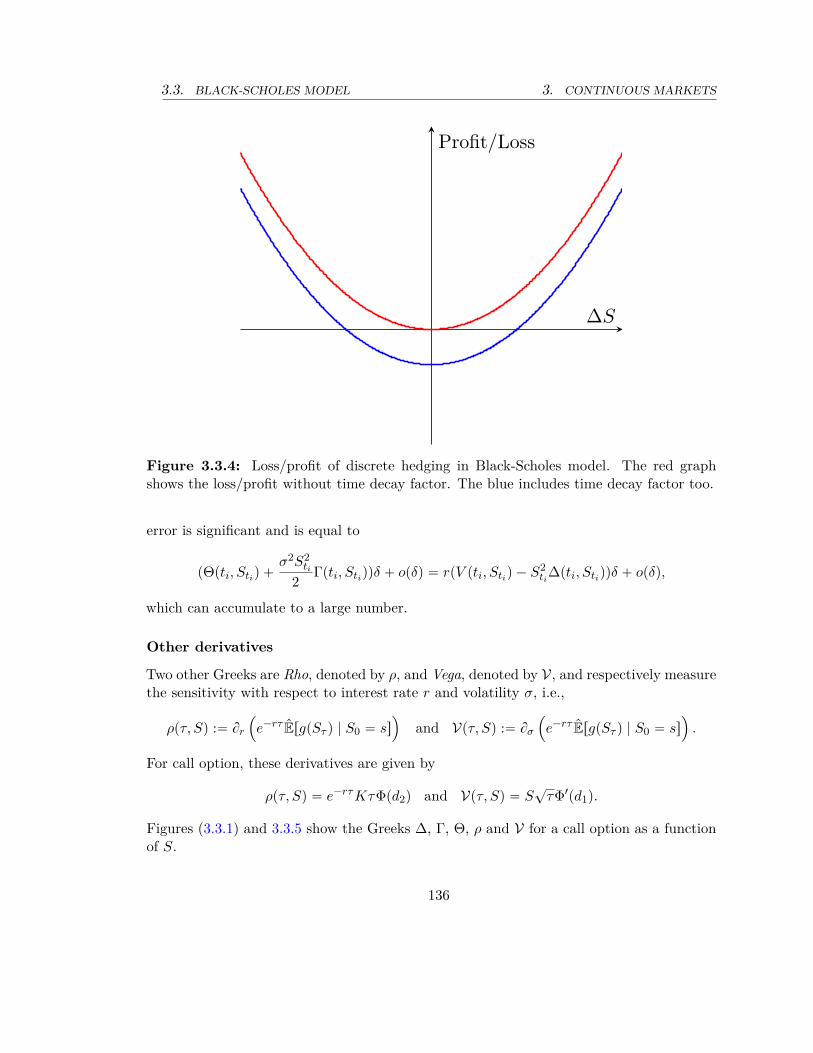
3.3. BLACK-SCHOLES MODEL 3. CONTINUOUS MARKETS
∆S
Profit/Loss
Figure 3.3.4: Loss/profit of discrete hedging in Black-Scholes model. The red graphshows the loss/profit without time decay factor. The blue includes time decay factor too.
error is significant and is equal to
pΘpti, Stiq `σ2S2
ti
2Γpti, Stiqqδ ` opδq “ rpV pti, Stiq ´ S2
ti∆pti, Stiqqδ ` opδq,
which can accumulate to a large number.
Other derivatives
Two other Greeks are Rho, denoted by ρ, and Vega, denoted by V, and respectively measurethe sensitivity with respect to interest rate r and volatility σ, i.e.,
ρpτ, Sq :“ Br
´
e´rτ ErgpSτ q | S0 “ ss
¯
and Vpτ, Sq :“ Bσ
´
e´rτ ErgpSτ q | S0 “ ss
¯
.
For call option, these derivatives are given by
ρpτ, Sq “ e´rτ KτΦpd2q and Vpτ, Sq “ S?
τΦ1pd1q.
Figures (3.3.1) and 3.3.5 show the Greeks ∆, Γ, Θ, ρ and V for a call option as a functionof S.
136

3. CONTINUOUS MARKETS 3.3. BLACK-SCHOLES MODEL
6 8 10 12 14
0
2
4
6
8
10
S
RhoVega
Figure 3.3.5: ρ and V of call option with τ “ 1, σ “ .1, r “ .05, and K “ 10.
Exercise 3.3.9. The third derivative of Black-Scholes price with respect to S is calledspeed. Find a closed form solution for speed.
Example 3.3.1. The payoff in Figure 3.3.6 can be written as pST ´ K1q` ´ pST ´ K2q` ´
pST ´ K3q` ` pST ´ K4q`. Therefore, the closed form solution for the Black-Scholes priceof the option is given by
V pτ, Sq “ Cpτ, K1, Sq ´ Cpτ, K2, Sq ´ Cpτ, K3, Sq ` Cpτ, K4, Sq.
All the Greeks of the option are also linear combination of these call option Greeks. For
K1 K2 K3 K4ST
g(ST )
Figure 3.3.6: Payoff of Example 3.3.1 gpST q “ pST ´ K1q` ´ pST ´ K2q` ´ pST ´ K3q` `
pST ´ K4q`.
instance,
∆pt, Sq “ Φpd1pτ, K1, Sqq ´ Φpd1pτ, K2, Sqq ´ Φpd1pτ, K3, Sqq ` Φpd1pτ, K4, Sqq.
137

3.3. BLACK-SCHOLES MODEL 3. CONTINUOUS MARKETS
Exercise 3.3.10. Write the payoffs in Figure 3.3.7 as linear combination of call optionsand derive a closed form formula for the Black-Scholes price, the Delta, and the Gamma ofthem. All the Greeks of the option are also linear combination of these call option Greeks.
KST
g(ST )
K1 K2 ST
g(ST )
Figure 3.3.7: Left: payoff of straddle. Right: payoff of strangle.
For instance,
∆pt, Sq “ Φpd1pτ, K1, Sqq ´ Φpd1pτ, K2, Sqq ´ Φpd1pτ, K3, Sqq ` Φpd1pτ, K4, Sqq.
Exercise 3.3.11 (Bull and bear call spreads). Write the following payoffs as linear com-bination of call options with different strikes and possibly some cash and give the closedform formula for them.
K1 K2ST
g(ST )
Figure 3.3.8: Red: Bull spread call. Blue: Bear spread call
138
3. CONTINUOUS MARKETS 3.3. BLACK-SCHOLES MODEL
3.3.6 Time-varying Black-Scholes model
Recall from Section 2.3 that the binomial model can be calibrated to the time dependentparameters. Let δ “ T
N and consider the discrete time instances ti “ iδ. Time-varyingbinomial can be given by
lnpStk`1q “ lnpSkδq ` lnpHk`1q,
where tHkuNk“1 is a sequence of independent random variables with the following distribu-
tion under risk-neutral probability
Hk “
#
1 ` δrtk`
?δσtk
αk with probability πk
1 ` δrtk´
?δσtk
βk with probability 1 ´ πk
,
where αk, βk are given by (2.3.4) and (2.3.5) for time dependent λt. Therefore, equation(3.3.4) takes the following time-dependent form:
lnpStkq “ lnpS0q `
k´1ÿ
i“0prti ´
σ2ti
2qδ `
?δ
Nÿ
k“1σtk
Zk. (3.3.17)
Analogous to (3.3.5), we have πk “βk
αk`βkand
ErZks “ 0 and ErZ2ks “ 1.
Therefore,
χ?δσtk
Zkpθq “ Ereiθσtk
Zk s “ 1 ` iθσtkδErZ1s ´
θ2σ2tk
δErZ21 s
2` opδq.
This implies that
χ?δřN
k“1 σtkZk
pθq “
Nź
k“1
ˆ
1 ´12
δθ2σ2tk
` opδ2q
˙
“
Nź
k“1e
´ 12 θ2σ2
tkδ`opδq “ e
´ θ22řN
i“1 σ2tk
δ`opδq.
As δ Ñ 0,χ?
δřN
k“1 σtkZk
pθq Ñ e´ θ22şT0 σ2
t dt,
which is the characteristic function of N p0,şT0 σ2
t dtq. Thus in the limit, we have
ST “ S0 expˆż T
0prt ´
σ2t
2qdt `
ż T
0σ2
t dtN p0, 1q
˙
.
139
3.3. BLACK-SCHOLES MODEL 3. CONTINUOUS MARKETS
As a matter of fact, for any t we have
St “ S0 expˆż t
0pru ´
σ2u
2qdu ` N
ˆ
0,
ż t
0σ2
udu
˙˙
ST “ St expˆż T
tpru ´
σ2u
2qdu ` N
ˆ
0,
ż T
tσ2
udu
˙˙
.
and the random variables N´
0,şTt σ2
udu¯
and N´
0,şt0 σ2
udu¯
are independent.Usually the interest rate rt and volatility σt are not given and we have to estimate them
from the data. In the next section, we discuss some estimation methods of these twoparameters.Using the variable r and σ, we can rewrite Black-Scholes formula for a call option by
CpT, K, S, tq :“ e´şTt ruduErpST ´ Kq` | St “ Ss “ SΦ pd1q ´ e´
şTt ruduKΦ pd2q ,
d1 “1
b
şTt σ2
udu
ˆ
lnpSKq `
ż T
t
ˆ
ru `σ2
u
2
˙
du
˙
and
d2 “1
b
şTt σ2
udu
ˆ
lnpSKq `
ż T
t
ˆ
ru ´σ2
u
2
˙
du
˙
.
For a general European payoff gpST q we have the Black-Scholes price given by
V pt, Sq :“ e´şTt ruduErgpSτ q | S0 “ Ss
“e´
şTt rudu
?2π
ż 8
´8
g
ˆ
S`
e´şTt pru´
σ2u2 qdu`x
b
şTt σ2
uudu˘˙
e´ x22 dx.
Remark 3.3.2. We shall see that in actual calculations, we only need to take one of theinterest rate rt or volatility σt time-varying!
3.3.7 Black-Scholes with yield curve and forward interest rate
Recall from Section 1.1.5 that the yield curve RtpT q and forward curve FtpT q of zero bondare defined by
BtpT q “ e´pT ´tqRtpT q “ e´şTt Ftpuqdu or or RtpT q :“ ´
1T ´ t
ln BtpT q FtpT q :“ ´d ln BtpT q
dT.
Since setting a model for forward rate is equivalent of setting a model for short rate rt,in Black-Scholes formula with varying interest rate, one can equivalently use the forwardrate or yield curve. Assume that σ is constant. Then, the Black-Scholes pricing formula
140

3. CONTINUOUS MARKETS 3.3. BLACK-SCHOLES MODEL
becomes
CpT, K, S, tq :“ e´şTt FtpuqduErpST ´ Kq` | St “ Ss “ SΦ pd1q ´ e´
şTt FtpuqduKΦ pd2q ,
d1 “1
a
σ2pT ´ tq
ˆ
lnpSKq `
ż T
tFtpuqdu `
σ2
2pT ´ tq
˙
and
d2 “1
a
σ2pT ´ tq
ˆ
lnpSKq `
ż T
tFtpuqdu ´
σ2
2pT ´ tq
˙
.
and
CpT, K, S, tq :“ e´RtpT qpT ´tqErpST ´ Kq` | St “ Ss “ SΦ pd1q ´ e´RtpT qpT ´tqKΦ pd2q ,
d1 “1
a
σ2pT ´ tq
ˆ
lnpSKq ` RtpT qpT ´ tq `σ2
2pT ´ tq
˙
and
d2 “1
a
σ2pT ´ tq
ˆ
lnpSKq ` RtpT qpT ´ tq ´σ2
2pT ´ tq
˙
.
(3.3.18)
3.3.8 Black-Scholes model and Brownian motion
In Section B.5, we show that symmetric random walk converges to the Brownian motionBt. The same principle shows that the linear interpolation of the summation
řNk“1 Zk in
logarithm of binomial model in (3.3.4), also converges to the Brownian motion. Therefore,one can write the Black-Scholes model (3.3.7) by using Brownian motion Bt; i.e.
St “ S0 expˆ
pr ´σ2
2qt ` σBt
˙
. (3.3.19)
The above process is called a geometric Brownian motion (GBM for short)9.
Markovian property of Black-Scholes model
Since for Brownian motion the increment Bs`t ´ Bt is independent of Bt,
St “ S0 expˆ
pr ´σ2
2qt ` σBt
˙
and St`s “ St expˆ
pr ´σ2
2qs ` σpBt`s ´ Btq
˙
are independent. Verbally, this means that the future movements of the price are indepen-dent of the past movements. In other words, given the history of the movements of asset
9Paul Samuelson first came with the idea of using GBM to model the risky asset price in 50’. The mainmotivation is that GBM never generates negative prices. Long before Samuelson on 1900, Louis Bacheliermodeled the price of a risky asset by a Brownian motion.
141
3.3. BLACK-SCHOLES MODEL 3. CONTINUOUS MARKETS
price until time t, i.e., Su for all u P r0, ts, the distribution of St`s only depends on St andthe part of history during u P r0, tq is irrelevant. As a result, for any function g : R` Ñ R,we have
ErgpSt`sq | Su : @u P r0, tss “ ErgpSt`sq | Sts “ E„
g
ˆ
St expˆ
pr ´σ2
2qs ` σpBt`s ´ Btq
˙˙ȷ
.
The pricing formula (3.3.9) is precisely derived form Markovian property of Black-Scholesmodel.As a result of Markovian property of GBM, one can write
St`dt ´ St “ St
ˆ
expˆ
pr ´σ2
2qdt ` σpBt`dt ´ Btq
˙
´ 1˙
“ St
´
pr ´σ2
2qdt ` σpBt`dt ´ Btq `
12
σ2pBt`dt ´ Btq2¯
` opdtq.
Therefore, the short term return of asset in Black-Scholes model is given by
St`dt ´ St
St“ pr ´
σ2
2qdt ` σpBt`dt ´ Btq `
12
σ2pBt`dt ´ Btq2 ` opdtq.
This is, in particular, consistent with Assumption 2.3.1 and the definition of mean returnand volatility, i.e.
E„
St`dt ´ St
St
ȷ
“ pr ´σ2
2qdt ` σErBt`dt ´ Bts `
12
σ2ErpBt`dt ´ Btq2s ` opdtq “ rdt ` opdtq.
var pSt`dt ´ StStq “ σ2dt ` opdtq.
Inspired from above formal calculation, We often write the Black-Scholes formula as
dSt
St“ rdt ` σdBt. (3.3.20)
The above equation which describes the dynamics of the price movements in Black-Scholesmodel is the differential form of writing (3.3.19).
Martingale property of Black-Scholes model
Similar to the binomial model, in the Black-Scholes model, the discounted asset price andthe discounted price of a European contingent claim are martingale. The discounted assetprice is Black-Scholes model is given by
St “ e´rtSt “ S0 expˆ
´σ2
2t ` σBt
˙
.
142
3. CONTINUOUS MARKETS 3.3. BLACK-SCHOLES MODEL
the conditional expectation of St`s given St is then given by
S0E„
expˆ
´σ2
2pt ` sq ` σBt`s
˙ˇ
ˇ
ˇ
ˇ
St
ȷ
“ S0 expˆ
´σ2
2t ` σBt
˙
E„
expˆ
´σ2
2s ` σpBt`s ´ Btq
˙ˇ
ˇ
ˇ
ˇ
St
ȷ
StE„
expˆ
´σ2
2s ` σpBt`s ´ Btq
˙ˇ
ˇ
ˇ
ˇ
St
ȷ
.
By the independence of the increments of Brownian motion, we have
E„
expˆ
´σ2
2s ` σpBt`s ´ Btq
˙ˇ
ˇ
ˇ
ˇ
St
ȷ
“ E„
expˆ
´σ2
2s ` σpBt`s ´ Btq
˙ȷ
,
and therefore,
E“
St`s
ˇ
ˇSt
‰
“ StE„
expˆ
´σ2
2s ` σpBt`s ´ Btq
˙ȷ
.
On the other hand since Bt`s ´ Bt „ N p0, sq, we have
E rexp pσpBt`s ´ Btqqs “ expˆ
σ2
2s
˙
,
and therefore, E“
St`s
ˇ
ˇSt
‰
“ St.Recall from formula (3.3.9) that the price of a contingent claim with payoff gpST q is given
byV pt, Stq “ e´rpT ´tqErgpST q | Sts.
If we define the discounted price by V pt, Stq “ e´rtV pt, Stq, then we can write the aboveas
V pt, Stq “ e´rT ErgpST q | Sts.
By the tower property of conditional expectation, we have
E“
V pt ` s, St`sqˇ
ˇSt
‰
“ E”
e´rT ErErgpST q | St`ss
ˇ
ˇ
ˇSt
ı
“ e´rT E rgpST q|Sts “ V pt, Stq.
Therefore, the price of the contingent claim is a martingale under risk-neutral probability.
3.3.9 Physical versus risk-neutral in Black-Scholes model
Recall that the price of an asset in the Black-Scholes model is represented by (3.3.20) orsimply
St “ S0 expˆ
pr ´σ2
2qt ` σBt
˙
.
143
3.3. BLACK-SCHOLES MODEL 3. CONTINUOUS MARKETS
This model is obtained by taking limit from the binomial model in the risk-neutral proba-bility framework. Therefore, the above representation is the risk-neutral price of the assetin Black-Scholes model. Indeed, one can see that the discounted price of the asset is amartingale, i.e.
e´rpt`sqErSt`s | Sts “ e´rtSt.
To show this one needs to use the fact that pBt`s ´ Bt and Bt are independent. Therefore,Bt`s ´ Bt and St are independent and we have
ErSt`s | Sts “ E„
St expˆ
pr ´σ2
2qs ` σpBt`s ´ Btq
˙ˇ
ˇ
ˇ
ˇ
St
ȷ
“ StE„
expˆ
pr ´σ2
2qs ` σpBt`s ´ Btq
˙ˇ
ˇ
ˇ
ˇ
St
ȷ
“ StE„
expˆ
pr ´σ2
2qs ` σpBt`s ´ Btq
˙ȷ
“ Ste´rsE
„
expˆ
´σ2
2s ` σpBt`s ´ Btq
˙ȷ
“ e´rsSt.
The last equality in the above is because Bt`s ´ Bt „ N p0, sq and EreσN p0,sqs “ e´ σ22 s.
Now recall the setting of Section 3.3.1, where we divide T units of time into N timesintervals, each of size δ :“ T
N . Then, consider a binomial model with N periods given bythe times t0 “ 0 ă t1 “ δ, ..., tk “ kδ, ...tN “ T . Then the binomial model under physicalprobability is given by
Spk`1qδ “ SkδHk`1, for k “ 0, ..., N ´ 1.
However, the distribution of the sequence of i.i.d. random variables tHkuNk“1 under physical
probability is now
Hk “
#
u with probability p
ℓ with probability 1 ´ p
Then, the dynamics of the asset price under physical probability is given by
lnpST q “ lnpS0q `
Nÿ
k“1lnpHkq.
lnpHkq is the log return Rlogkδ . Recall from (3.3.3) that the first two moments of log return
are given by
ErlnpHkqs “ pµ ´12
σ2qδ ` Opδ2q, ErlnpHkq2s “ σ2δ ` opδq
144
3. CONTINUOUS MARKETS 3.3. BLACK-SCHOLES MODEL
In other words, if we define Z 1k :“ lnpHkq´pµ´σ22q
σ?
δ, one can write
lnpST q “ lnpS0q `
ˆ
µ ´12
σ2˙
T ` σ?
T ¨1
?N
Nÿ
k“1Z 1
k,
where tZ 1ku is a sequence of i.i.d. random variables satisfying
ErZ 1ks “ opδq, and ErpZ 1
kq2s “ 1 ` op1q.
If follows from (3.3.6) that 1?N
řNk“1 Z 1
k converges weakly to N p0, 1q, and under physicalprobability, the Black-Scholes model is described by
St “ S0 expˆ
pµ ´σ2
2qt ` σBt
˙
.
In other words, by switching from risk-neutral probability to physical probability, we adjustthe mean return of the asset from r to the risk-free interest rate µ.
Remark 3.3.3. For the purpose of derivative pricing, the physical probability is irrelevant.This is because by the fundamental theorem of asset pricing, Theorem 1.3.1, the price ofany derivative is determined by the discounted expectation of payoff under risk-neutral prob-ability. However, for portfolio management the physical probability is important, becauseit carries the long-term growth rate of the asset µ. For example, an investor with x initialwealth wants to decide how to split his investment between risk-free bond with interest rater and a risky asset given by Black-Scholes equation
St “ S0 expˆ
pµ ´σ2
2qt ` σBt
˙
.
His objective is to maximize his expected wealth at time T subject to a constraint of the riskof portfolio measured by the variance of the wealth at time T , i.e.
maxθ
tErXθT s ´ λvarpXθ
T qu. (3.3.21)
where XθT is the wealth of the investor at time T if he chooses to invest x0 ´ θ on risk-free
asset and θ on risky asset. The wealth XθT satisfies
XθT “ erT px0 ´ θq ` θepµ´ σ2
2 qT `σBT .
Therefore,
ErXθT s “ erT px0 ´ θq ` θeµ and varpXθ
T q “ θ2e2µT peσ2T ´ 1q.
145
3.3. BLACK-SCHOLES MODEL 3. CONTINUOUS MARKETS
Therefore, the portfolio maximization problem (3.3.21) is given by
maxθ
!
erT px0 ´ θq ` θeµT ´ λθ2e2µT peσ2T ´ 1q
)
.
and the solution is given by
θ˚ “eµT ´ erT
2λe2µT peσ2T ´ 1q.
Volatility estimation
Notice that the log return of the Black-Scholes model satisfies
ln´St`δ
St
¯
“ pµ ´σ2
2qδ ` σpBt`δ ´ Btq
We consider the time discretization t0 “ 0 and ti`1 “ ti ` δ and tN “ t. Therefore, iffollows form (B.14) (quadratic variation of Brownian motion) that
N´1ÿ
i“0ln´Sti`1
Sti
¯2“ σ2
N´1ÿ
i“0pBti`1 ´ Btiq
2 ` opδq Ñ σ2t (3.3.22)
One can use (3.3.22) to make an estimation of volatility. For any ti “ iδ evaluate
Yti :“i´1ÿ
j“0ln´Stj`1
Stj
¯2.
If δ is small enough, then Yti should approximately be equal to tiσ2. This suggests that if
we fit a line to the data tpti, Ytiq : i “ 0, 1, ...u. Then, the slope of line is σ2. The schematicpicture of this fitting is shown in figure 3.3.9.
Exercise 3.3.12 (Project). With the same set of data from Exercise 2.3.1, calculate thevolatility by using the quadratic variation formula (3.3.22). Take δ “ 1
250 year. Then, plotthe estimated quadratic variation Yti versus time ti. Some examples of the the generatedplots is given in Figure 3.3.10. Then fit a line to the data by assuming Yt “ σ2t ` noise.To fit a line to the data points, you can use least square method. The slope of the line givesyou the volatility σ.
3.3.10 Black-Scholes equation
Recall from Proposition 3.3.1 that the price V pτ, Sq of the Markovian European contingentclaim with payoff gpST q at time t “ T ´ τ (τ is time-to-maturity) when the asset price is
146

3. CONTINUOUS MARKETS 3.3. BLACK-SCHOLES MODEL
0 0.5 1
Time
Quad
raticvariationof
logreturn data
fitted line: Slope=σ2
Figure 3.3.9: Quadratic variation estimation of volatility
0 0.5 1
0.1
0.2
Time
Quad
raticvariationof
logreturn
0 0.5 1
0
1
2
3·10−2
Time
Figure 3.3.10: Quadratic variation estimation of volatility: Left: Tesla motors. Right:S&P500
S satisfies´Bτ V pτ, Sq “ ´
σ2S2
2BSSV pτ, Sq ´ rSBSpτ, Sq ` rV pτ, Sq.
The above equation is a partial differential equation called Black-Scholes equation. One wayto find the pricing formula for an option is to solve the Black-Scholes PDE. As all PDEsa boundary condition and a initial condition10 is required to solve a PDE analyticallyor numerically. The initial condition for the Black-Scholes equation is the payoff of thederivative, i.e.
V p0, Sq “ gpSq.
10For time-dependent PDEs.
147
3.3. BLACK-SCHOLES MODEL 3. CONTINUOUS MARKETS
Notice that here when τ “ 0, we have t “ T .Notice that the above PDE holds in region τ P r0, T s and S ą 0. Therefore, we need a
boundary condition at S “ 0. This boundary condition is a little trick to make, becausein Black-Scholes model, the price of the asset St never hits zero, i.e., if price of an assetis initially positive, then the price stays positive at all times. If an asset is price less, theprice stays zero at all time. Therefore, if the price of the asset is initially 0, then ST “ 0and the price of the option with payoff gpST q is given by
V pτ, 0q “ e´rτ ErgpST q | ST ´τ “ 0s “ e´rτ gp0q.
Therefore, the boundary condition for at S “ 0 is given by
V pτ, 0q “ e´rτ gp0q.
To summarize, the Black-Scholes PDE for pricing Markovian European contingent claimwith payoff gpST q is given by the following boundary value problem
$
’
&
’
%
Bτ V pτ, Sq “ σ2S2
2 BSSV pτ, Sq ` rSBSV pτ, Sq ´ rV pτ, Sq
V pτ, 0q “ e´rτ gp0q
V p0, Sq “ gpSq
. (3.3.23)
Exercise 3.3.13. Consider the option with payoff gpST q “ 1?ST
. Find the Black-Scholesprice of this payoff at time t “ 0 by solving PDE (3.3.23). Hint: Try to plug in V pτ, Sq “
e´rτ Sa into the Black-Scholes equation, for some constant a. Then, find the constant a.The boundary condition V pτ, 0q “ e´rτ gp0q is unnecessary as gp0q “ 8.
Remark 3.3.4. The boundary condition V pτ, 0q “ e´rτ gp0q is some how redundant inequation (3.3.23). Because in the Black-Scholes model, the price of underlying asset neverhits zero. But, this condition is important for solving Black-Scholes equation numerically.
Heat equation and Black-Scholes model
Recall from Exercise 3.3.8 that the change of variable S :“ e´rpT ´τqS and V pτ, Sq :“e´rpT ´τqV pτ, Sq “ e´rpT ´τqV pτ, erpT ´τqSq modifies the Black-Scholes equation to
Bτ V pτ, Sq “σ2S2
2BSSV pτ, Sq.
If we make a change of variable x :“ lnpSq and Upτ, xq :“ V pτ, exq, then we obtain theheat equation
Bτ Upτ, xq “σ2
2BxxUpτ, xq.
148

3. CONTINUOUS MARKETS 3.3. BLACK-SCHOLES MODEL
Unlike (3.3.23), the heat equation holds on the whole space, i.e.#
Bτ Upτ, xq “ σ2
2 BxxUpτ, xq
Up0, xq “ e´rT V perT exq. (3.3.24)
Notice that at time t “ 0 (or τ “ T ), the price of the the Markovian European contingentclaim with payoff gpST q is equal to V pT, S0q “ V pT, S0q “ UpT, lnpS0qq.Transforming the Black-Scholes equation into heat equation helps us to use numerical
techniques from heat equation in Section 3.2.2 for Black-Scholes equation.
Solving Black-Scholes equation via finite-difference scheme for Black-Scholesequation
One can directly discretize Black-Scholes equation (3.3.23) to apply finite difference methoddescribed in the previous section. See Figure 3.3.11 In this case, the computation domainhas to be r0, Smaxs for some Smax ą 0. The boundary condition at 0 is already assigned at(3.3.23) by
V pτ, 0q “ e´rτ gp0q,
and the ABC at Smax is given by the growth of the payoff for large values of S. For theexample of call option, the ABC is
V pt, Smaxq “ Smax for Smax sufficiently large.
The rest of the approximation goes the same as the previous section. However, one shouldbe cautious about applying the explicit schemes which need CFL condition. Recall thatThe right-hand side of CFL condition is always 1
2 times the inverse of the coefficient ofsecond derivative in the equation. Therefore, CFL condition translates to
h
k2 ď1
σ2S2 .
If Smax is very large, for a fixed space discretization k, one needs to set h very small. Thedownside of this method is that the time of the algorithm increases significantly.
Binomial tree scheme for Black-Scholes
Recall from Section 3.3.1 that the Black-Scholes model is the limit of binomial modelunder risk-neutral probability. Therefore, if necessary, one can use the binomial modelto approximate the Black-Scholes price of the contingent claim. For implementation, oneneeds to choose a sufficiently large number of periods N , or equivalently a small δ “ T
N .Suggested by (3.3.1), for a given interest rate r and volatility σ, we need to choose u and
149

3.3. BLACK-SCHOLES MODEL 3. CONTINUOUS MARKETS
Smax
S
tT
k
h
Figure 3.3.11: Finite difference grid for Black-Scholes equation. In the explicit schemethe CFL condition should be satisfied, i.e., h
k2 ď 1σS . This requires a choice of very small
h. Artificial boundary conditions are necessary on both Smax and 0.
ℓ and the one period interest rate R as follows.
u “ eδpr´ σ22 q`
?δσα, l “ eδpr´ σ2
2 q´?
δσβ , and R “ rδ,
where α and β are given by (2.3.4). However, one can avoid the calculation of α and β bymaking some different choices. Notice that the binomial model has three parameters u, ℓand R while the Black-Scholes parameters are only two. This degree of freedom providesus with some modifications of binomial three which still converges to the Black-Scholesformula. This also simplifies the calibration process in Section 2.3 significantly simpler.Here are some choices:
a) Symmetric probability:
u “ eδpr´ σ22 q`
?δσ, l “ eδpr´ σ2
2 q´?
δσ, and R “ rδ,
Then;πu “ πℓ “
12
.
b) Subjective return:
u “ eδν`?
δσ, l “ eδν´?
δσ, and R “ rδ,
150
3. CONTINUOUS MARKETS 3.3. BLACK-SCHOLES MODEL
Then;
πu “12
˜
1 `?
δr ´ ν ´ 1
2σ2
σ
¸
and πℓ “12
˜
1 ´?
δr ´ ν ´ 1
2σ2
σ
¸
.
To see why this choices work, recall (3.3.4) from Section 3.3.1. The only criteria for theconvergence of binomial model to Black-Scholes model is that when we write the log ofasset price in binomial model as in (3.3.4),
lnpST q “ lnpS0q ` pr ´σ2
2qT ` σ
?T ¨
1?
N
Nÿ
k“1Zk,
the random variables Zk, k “ 1, ..., N must satisfy
ErZ1s “ opδq, and ErZ21 s “ 1 ` op1q.
In the Section 3.3.1, we made a perfect choice of ErZ1s “ 0 and ErZ21 s “ 1.
Monte Carlo scheme for Black-Scholes
Recall from Section 3.3.2 that the price of a Markovian European contingent claim can bewritten as an expectation or/and a single integral.
V pτ, Sq :“ e´rτ ErgpSτ q | S0 “ Ss “e´rτ
?2π
ż 8
´8
g
ˆ
S`
epr´ σ22 qτ`σ
?τx˘
˙
e´ x22 dx.
One way to estimate V pT, S0q is to generate a sample xp1q, ..., xpMq of N p0, 1q and approx-imate the above expectation by
e´rT
M
Mÿ
j“1g
ˆ
S0`
epr´ σ22 qT `σ
?T xpjq˘
˙
.
Another method of approximation is to directly target the integral by choosing a largenumbers 0 ă xmax and approximate the integral by a finite Riemann sum. More precisely,let ∆x :“ xmax
L and xpjq “ j∆x. The the approximation goes as follows.
e´rTL´1ÿ
j“´L
g
ˆ
S0`
epr´ σ22 qT `σ
?T xpjq
˘
˙
e´x2
pjq
2 ∆x.
There are more complicated and efficient Monte Carlo schemes and integration methodswhich we do not discuss here.
151

3.3. BLACK-SCHOLES MODEL 3. CONTINUOUS MARKETS
Exercise 3.3.14 (Project). Consider a payoff bull spread call in Figure 3.3.8 with T “ 1,K1 “ 10 and K2 “ 20. Assume that the parameters of the underlying asset are given byS0 “ 15, σ “ .02, and the interest rate is r “ .01 (1%). We know the actual value of thisoption from Black-Scholes formula. Now, compare the following estimation schemes forthe price of bull spread call. Record the time of the algorithms for each scheme to obtainthe four digit accuracy.
a) Implicit finite-difference with parameter θ “ .5.
b) Implicit finite-difference with parameter θ “ 1.
c) Explicit finite difference (equivalently implicit with θ “ 0).
d) Symmetric binomial model.
e) Monte Carlo scheme.
f) Approximation by a Riemann sum.
3.3.11 Stock price with dividend in Black-Scholes model
Here we consider two types of dividend strategies. If the dividend is paid continuously,then there is a constant outflow of cash from the price of the asset. If the rate of dividendpayment is Dt, the Black-Scholes model in (3.3.20) has to be modified to
dSt “ rStdt ` σdBt ´ Dtdt.
Choosing Dt :“ qSt for q ě 0, we obtain
dSt “ pr ´ qqStdt ` σStdBt.
Remark 3.3.5. For a continuous dividend rate q the dividend yield in time period rt, T s
is given by e´qpT ´tq ˆ 100 percent.
Especially, this choice guarantees that the dividend is always less than the asset price andpaying dividend does not diminish the value of the asset. In the exponential form we have
St “ S0 exp ppr ´ qqt ` σBtq “ e´qtS0 expˆ
pr ´σ2
2qt ` σBt
˙
.
In this case, the Black-Scholes price of a European contingent claim with payoff gpST q isgiven by
V pt, Sq “ e´rpT ´tqErgpST q | St “ Ss “ e´rpT ´tqE”
g´
e´qpT ´tqST
¯
| St “ Sı
,
152
3. CONTINUOUS MARKETS 3.3. BLACK-SCHOLES MODEL
where St satisfies the Black-Scholes equation without dividend, i.e.
St “ S0 expˆ
pr ´σ2
2qt ` σBt
˙
.
If the dividend strategy is time-varying qt, then one can write the above pricing formula as
V pt, Sq “ e´rpT ´tqE”
g´
e´şTt qsdsST
¯
| St “ Sı
,
For the continuous rate of dividend, the relation between Greeks of the option in Propo-sition 3.3.1 is modified as in the following proposition.
Proposition 3.3.2. Let St follow Black-Scholes price with continuous dividend rate q. Fora European Markovian contingent claim, the Black-Scholes price satisfies
Θpτ, Sq “ ´σ2S2
2Γpτ, Sq ´ pr ´ qqS∆pτ, Sq ` rV pτ, Sq.
Second type of dividend strategy is a discrete one. The discrete dividend is paid in times0 ď t0 ă t1 ă ... ă tN ď T in amounts D0, ..., DN . Then, between the time of dividendpayments, the asset price follows the Black-Scholes model, i.e.
St “ Stn´1 expˆ
pr ´σ2
2qpt ´ tn´1q ` σpBt ´ Btn´1q
˙
, t P rtn´1, qtns.
Just a moment before the payment of dividend at time tn´11 the price of the asset is
Stn´ :“ Stn´1 expˆ
pr ´σ2
2qptn ´ tn´1q ` σpBtn ´ Btn´1q
˙
.
But after paying Dn for dividend, this price reduces to
Stn “ Stn´ ´ Dn “ Stn´1 expˆ
pr ´σ2
2qptn ´ tn´1q ` σpBtn ´ Btn´1q
˙
´ Dn.
As mentioned in Section 2.2.4, the dividend is usually given as a percentage of the currentasset price, i.e.
Dn “ dnStn´, with dn P r0, 1q.
and we have
Stn “ p1 ´ dnqStn´ “ p1 ´ dnqStn´1 expˆ
pr ´σ2
2qptn ´ tn´1q ` σpBtn ´ Btn´1q
˙
.
11The moment before time t is denoted by t´.
153
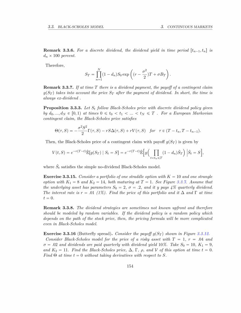
3.3. BLACK-SCHOLES MODEL 3. CONTINUOUS MARKETS
Remark 3.3.6. For a discrete dividend, the dividend yield in time period rtn´1, tns isdn ˆ 100 percent.
Therefore,
ST “
Nź
n“1p1 ´ dnqS0 exp
ˆ
pr ´σ2
2qT ` σBT
˙
.
Remark 3.3.7. If at time T there is a dividend payment, the payoff of a contingent claimgpST q takes into account the price ST after the payment of dividend. In short, the time isalways ex-dividend .
Proposition 3.3.3. Let St follow Black-Scholes price with discrete dividend policy givenby d0, ..., dN P r0, 1q at times 0 ď t0 ă t1 ă ... ă tN ď T . For a European Markoviancontingent claim, the Black-Scholes price satisfies
Θpτ, Sq “ ´σ2S2
2Γpτ, Sq ´ rS∆pτ, Sq ` rV pτ, Sq for τ P pT ´ tn, T ´ tn´1q.
Then, the Black-Scholes price of a contingent claim with payoff gpST q is given by
V pt, Sq “ e´rpT ´tqErgpST q | St “ Ss “ e´rpT ´tqE”
g´
ź
tătnďT
p1 ´ dnqST
¯ ˇ
ˇ
ˇSt “ S
ı
,
where St satisfies the simple no-dividend Black-Scholes model.
Exercise 3.3.15. Consider a portfolio of one straddle option with K “ 10 and one strangleoption with K1 “ 8 and K2 “ 14, both maturing at T “ 1. See Figure 3.3.7. Assume thatthe underlying asset has parameters S0 “ 2, σ “ .2, and it y pays 4% quarterly dividend.The interest rate is r “ .01 (1%). Find the price of this portfolio and it ∆ and Γ at timet “ 0.
Remark 3.3.8. The dividend strategies are sometimes not known upfront and thereforeshould be modeled by random variables. If the dividend policy is a random policy whichdepends on the path of the stock price, then, the pricing formula will be more complicatedeven in Black-Scholes model.
Exercise 3.3.16 (Butterfly spread). Consider the payoff gpST q shown in Figure 3.3.12.Consider Black-Scholes model for the price of a risky asset with T “ 1, r “ .04 and
σ “ .02 and dividends are paid quarterly with dividend yield 10%. Take S0 “ 10, K1 “ 9,and K2 “ 11. Find the Black-Scholes price, ∆, Γ, ρ, and V of this option at time t “ 0.Find Θ at time t “ 0 without taking derivatives with respect to S.
154
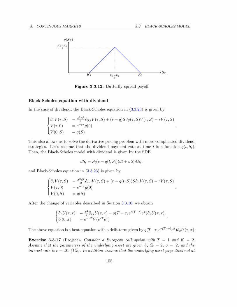
3. CONTINUOUS MARKETS 3.3. BLACK-SCHOLES MODEL
K1 K2K1+K2
2
K2−K1
2
ST
g(ST )
Figure 3.3.12: Butterfly spread payoff
Black-Scholes equation with dividend
In the case of dividend, the Black-Scholes equation in (3.3.23) is given by$
’
&
’
%
Bτ V pτ, Sq “ σ2S2
2 BSSV pτ, Sq ` pr ´ qqSBSpτ, SqV pτ, Sq ´ rV pτ, Sq
V pτ, 0q “ e´rτ gp0q
V p0, Sq “ gpSq
.
This also allows us to solve the derivative pricing problem with more complicated dividendstrategies. Let’s assume that the dividend payment rate at time t is a function qpt, Stq.Then, the Black-Scholes model with dividend is given by the SDE
dSt “ Stpr ´ qpt, Stqqdt ` σStdBt.
and Black-Scholes equation in (3.3.23) is given by$
’
&
’
%
Bτ V pτ, Sq “ σ2S2
2 BSSV pτ, Sq ` pr ´ qpt, SqqSBSV pτ, Sq ´ rV pτ, Sq
V pτ, 0q “ e´rτ gp0q
V p0, Sq “ gpSq
.
After the change of variables described in Section 3.3.10, we obtain#
Bτ Upτ, xq “ σ2
2 BxxUpτ, xq ´ qpT ´ τ, erpT ´τqexqBxUpτ, xq,
Up0, xq “ e´rT V perT exq.
The above equation is a heat equation with a drift term given by qpT ´τ, erpT ´τqexqBxUpτ, xq.
Exercise 3.3.17 (Project). Consider a European call option with T “ 1 and K “ 2.Assume that the parameters of the underlying asset are given by S0 “ 2, σ “ .2, and theinterest rate is r “ .01 (1%). In addition assume that the underlying asset pays dividend at
155
3.3. BLACK-SCHOLES MODEL 3. CONTINUOUS MARKETS
continuous rate qpt, Stq “ .05e´.01tSt, i.e., 5% of the discounted asset price at each time.
a) Write the Black-Scholes equation for this problem and convert it into heat equationwith a drift term.
b) Solve this problem numerically by using a finite difference scheme.
Example 3.3.2. Consider a European option with payoff
gpST q “ eαST .
Assume that the the interest rate is r ą 0 and the volatility of the underlying asset is σ ą 0,and at time 0, it has value S0, and pays dividend at continuous rate equal to qpt, Stq “ qSt,where q ą 0. Then, the Black-Scholes equation is given by
#
Bτ V pτ, Sq “ σ2S2
2 BSSV pτ, Sq ` pr ´ qSqSBSV pτ, Sq ´ rV pτ, Sq
V p0, Sq “ eαS ..
The boundary condition for Black-Scholes equation at S “ 0 is given by
V pτ, 0q “ 1.
Function V pτ, Sq “ e´rτ eαS satisfies the Black-Scholes equation and the boundary condi-tions. Therefore, the price of the contingent claim with payoff eαST at time-to-maturity τ(at time T ´ τ) is given by V pτ, Sq “ e´rτ eαS if the asset price takes value S at time time.
Exercise 3.3.18. Consider a European option with payoff
gpST q “ S´5T e10ST .
Assume that the the interest rate is r “ .1 and the underlying asset satisfies S0 “ 2, σ “ .2,and pays dividend at continuous rate equal to qpt, Stq “ .2St.
a) Write the Black-Scholes equation for this problem.
b) Solve this problem analytically by the method of separation of variables. Plug into theequation a solution candidate of the form eατ S´5e10S and determine α.
156

3. CONTINUOUS MARKETS3.4. TERM STRUCTURE OF THE VOLATILITY AND VOLATILITY SMILE
3.4 Term structure of the volatility and volatility smile
For simplicity we assume that the interest rate is estimated to be constant. Then, givenconstant volatility σ, the call option price is given by Black-Scholes formula.
Cpτ, K, S, σ, rq :“ SΦ pd1q ´ e´rτ KΦ pd2q ,
d1 “1
σ?
τ
ˆ
lnpSKq ` pr `σ2
2qτ
˙
and d2 “1
σ?
τ
ˆ
lnpSKq ` pr ´σ2
2qτ
˙
.
Since BσCpτ, K, S, σ, rq “: V “ S?
τΦ1pd1q is positive, then Cpτ, K, S, σ, rq is strictly in-creasing on σ. In addition, we have
limσÓ0
Cpτ, K, S, σ, rq “ pS ´ e´rτ Kq` and limσÒ8
Cpτ, K, S, σ, rq “ S.
The following exercise shows that the price quotes of call option should be in the rangerpS ´ e´rτ Kq`, Ss, independent of the model.Recall from Section 1.2 that the price of a call option satisfies
pS ´ BtpT qKq` ď CpT, K, S, tq ď S.
independent of the model. Therefore, for any price quote C˚pτ, K, Sq of call option withstrike K and time-to-maturity τ , there exists a unique σimppτ, K, Sq such that
Cpτ, K, S, σimp, rq “ C˚pτ, K, Sq.
σimppτ, K, Sq is called implied volatility. See Figure 3.4.1Knowing S, σimp is a function of τ and K. If Black-Scholes model is true, σimp must be a
constant function, however this is not compatible with the data. For example, Figure 3.4.2shows the implied volatility for Tesla motor stock price which obviously is not constant.For closer maturities, the volatility is larger than later maturities. In addition, for nearlyATM options, K « $175, the volatility is larger. In Figure 3.4.3, we isolated some cross-sections of the volatility surface for time-to-maturity equal to 2 weeks and 4 months andstrike price equal to $185.
Exercise 3.4.1 (Project). Go to google finance, yahoo finance or any other database whichprovides free option price data for one instant of time. In google finance it is often referredto as option chain. Pick a stock which has a rich option chain with many quotes for differentmaturities and strike, such as IBM, Apple, Alphabet, FB, etc. Then, single out rows ofoption price quotes which exhibit most recent option price which show large values in tradedvolume and open interest. See Table 3.1.Choose interest rate r from the data given on Table 3.2. Try to use options with maturities
as close as possible to the maturity of the yield curve for more accurate estimation.
157

3.4. VOLATILITY SMILE 3. CONTINUOUS MARKETS
σimp(τ ,K)
(S − e−rτK)+
C∗(τ ,K)
S
σ
C(τ,K, σ)
Figure 3.4.1: Implied volatility: the price of call option in Black-Scholes model is mono-tone on volatility σ.
170
180
190
200
210
220
few days
1 Mo1.5 Mo
4 Mo
.2
.4
.6
.8
K
τ
Implied
vola
tiltiy
Figure 3.4.2: Implied volatility surface at Feb 24, 2016 for Tesla stock NASDAQ:TSLA.
Then, use Newton-Raphson method or bisection method to approximate the implied volatil-ity from the call option data. Since you have yield curve data, use (3.3.18) as the Black-Scholes pricing formula.Create a chart similar to the one below to insert the implied volatil-ity inside.
158
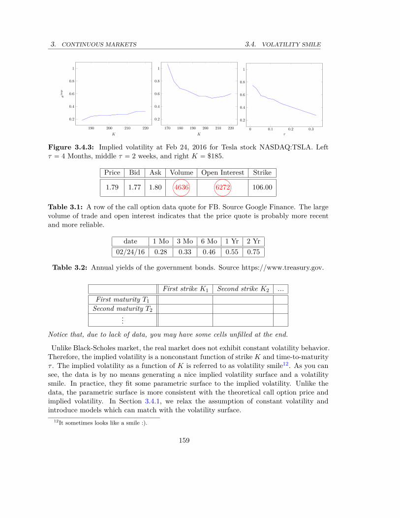
3. CONTINUOUS MARKETS 3.4. VOLATILITY SMILE
190 200 210 220
0.2
0.4
0.6
0.8
1
K
σim
p
170 180 190 200 210 220
0.2
0.4
0.6
0.8
1
K
0 0.1 0.2 0.3
0.2
0.4
0.6
0.8
1
τ
Figure 3.4.3: Implied volatility at Feb 24, 2016 for Tesla stock NASDAQ:TSLA. Leftτ “ 4 Months, middle τ “ 2 weeks, and right K “ $185.
Price Bid Ask Volume Open Interest Strike
1.79 1.77 1.80 4636 6272 106.00
Table 3.1: A row of the call option data quote for FB. Source Google Finance. The largevolume of trade and open interest indicates that the price quote is probably more recentand more reliable.
date 1 Mo 3 Mo 6 Mo 1 Yr 2 Yr02/24/16 0.28 0.33 0.46 0.55 0.75
Table 3.2: Annual yields of the government bonds. Source https://www.treasury.gov.
First strike K1 Second strike K2 ...First maturity T1
Second maturity T2...
Notice that, due to lack of data, you may have some cells unfilled at the end.
Unlike Black-Scholes market, the real market does not exhibit constant volatility behavior.Therefore, the implied volatility is a nonconstant function of strike K and time-to-maturityτ . The implied volatility as a function of K is referred to as volatility smile12. As you cansee, the data is by no means generating a nice implied volatility surface and a volatilitysmile. In practice, they fit some parametric surface to the implied volatility. Unlike thedata, the parametric surface is more consistent with the theoretical call option price andimplied volatility. In Section 3.4.1, we relax the assumption of constant volatility andintroduce models which can match with the volatility surface.
12It sometimes looks like a smile :).
159
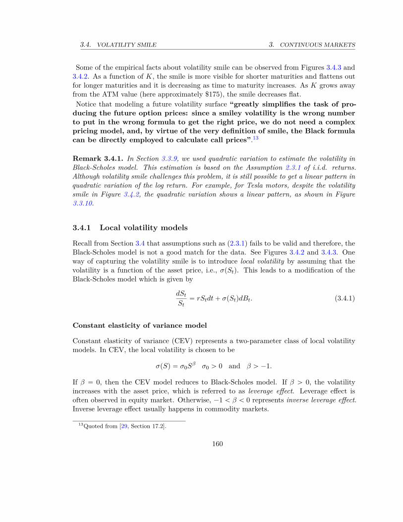
3.4. VOLATILITY SMILE 3. CONTINUOUS MARKETS
Some of the empirical facts about volatility smile can be observed from Figures 3.4.3 and3.4.2. As a function of K, the smile is more visible for shorter maturities and flattens outfor longer maturities and it is decreasing as time to maturity increases. As K grows awayfrom the ATM value (here approximately $175), the smile decreases flat.Notice that modeling a future volatility surface “greatly simplifies the task of pro-
ducing the future option prices: since a smiley volatility is the wrong numberto put in the wrong formula to get the right price, we do not need a complexpricing model, and, by virtue of the very definition of smile, the Black formulacan be directly employed to calculate call prices”.13
Remark 3.4.1. In Section 3.3.9, we used quadratic variation to estimate the volatility inBlack-Scholes model. This estimation is based on the Assumption 2.3.1 of i.i.d. returns.Although volatility smile challenges this problem, it is still possible to get a linear pattern inquadratic variation of the log return. For example, for Tesla motors, despite the volatilitysmile in Figure 3.4.2, the quadratic variation shows a linear pattern, as shown in Figure3.3.10.
3.4.1 Local volatility models
Recall from Section 3.4 that assumptions such as (2.3.1) fails to be valid and therefore, theBlack-Scholes model is not a good match for the data. See Figures 3.4.2 and 3.4.3. Oneway of capturing the volatility smile is to introduce local volatility by assuming that thevolatility is a function of the asset price, i.e., σpStq. This leads to a modification of theBlack-Scholes model which is given by
dSt
St“ rStdt ` σpStqdBt. (3.4.1)
Constant elasticity of variance model
Constant elasticity of variance (CEV) represents a two-parameter class of local volatilitymodels. In CEV, the local volatility is chosen to be
σpSq “ σ0Sβ σ0 ą 0 and β ą ´1.
If β “ 0, then the CEV model reduces to Black-Scholes model. If β ą 0, the volatilityincreases with the asset price, which is referred to as leverage effect. Leverage effect isoften observed in equity market. Otherwise, ´1 ă β ă 0 represents inverse leverage effect.Inverse leverage effect usually happens in commodity markets.
13Quoted from [29, Section 17.2].
160

3. CONTINUOUS MARKETS 3.4. VOLATILITY SMILE
Calibration of local volatility models
Calibration of local volatility models is not an easy job. For example, assume that we knowthe volatility is given by function σpStq. Then, the quadratic variation of the asset price isgiven by a formula similar to (3.3.22), i.e., for time discretization t0 “ 0 and ti`1 “ ti ` δand tN “ t, we have
N´1ÿ
i“0ln´Sti`1
Sti
¯2“
N´1ÿ
i“0σ2pStiqpBti`1 ´ Btiq
2 ` opδq Ñ
ż t
0σ2pSuqdu. (3.4.2)
Unlike (3.3.22), where the limit is σ2t, the right-hand side above is random, because Su israndom. One may think of trying to regress the summation of log returns on the discretizedpath S0, St1 , ..., StN´1 in order to see some pattern. However, this is a high dimensionalregression which is not a good idea. A better idea could be to plot
ln´Sti`1
Sti
¯2“ σ2pStiqpBti`1 ´ Btiq
2 ` op1q.
against St to see if there is a pattern. The pattern can suggest a shape for the functionσ2pSq. Notice that the pBti`1 ´ Btiq
2 term in the above right-hand side is δ times a χ2
random variable. This makes it impossible to apply simple statistical estimations. Onthe other hand, the a simple experiment shows that it sometimes fails to give a reliablepattern. For instance, Figure 3.3.10 shows a clear pattern of approximately linear growthin the quadratic variation of log return against time. If we try to do the same thing againstthe stock price St, we get Figure 3.4.4.A better way to calibrate local volatility model is to go back to where it is coming from,
i.e., the volatility surface. A famous work of Bruno Dupire in [11] (see also [18])gives thelocal volatility which matches with the volatility surface.
Theorem 3.4.1 (Dupire’s theorem). Suppose that at time t the underlying asset price is S.In addition, the volatility surface is given, i.e., all call prices are given by CpK, T, S, tq.Then,there is at most one local volatility model which matches with the given call prices. In thiscase, the volatility is given by
σ2pt, sq “ 2BT C ` rKBKC
K2BKKC
ˇ
ˇ
ˇ
ˇ
pT,Kq“pt,sq
,
provided that the derivatives BT C, BKC, and BKKC exists.
As seen from Exercise 1.2.3, CpT, K, S, tq is convex with respect to K. Therefore, for thedenominator we have K2BKKCKK ě 0. The following exercise shows that independent ofmodel, the numerator BT C ` rKBKC ě 0. Here we assume that the risk-free interest rateis constant r.
161

3.4. VOLATILITY SMILE 3. CONTINUOUS MARKETS
140 160 180 200 220 240 260 280
0
1
2
3
S
Quad
raticvariationof
logreturn
1,800 1,850 1,900 1,950 2,000 2,050 2,100 2,150
0
0.1
0.2
0.3
0.4
S
Figure 3.4.4: Plot of quadratic log return ln´
Sti`1Sti
¯2against St. Left: Tesla motors.
Right: S&P500.
Exercise 3.4.2. Show that
CpT ` δ, BT pT ` δqK, S, tq ě CpT, K, S, tq.
Therefore, the task of calibration can be simplified if we choose to fit a differentiable volsurface to the implied volatility data which satisfies the following conditions
a) K2BKKCKK ą 0.
b) BT C ` rKBKC ě 0.
In addition, if the volatility surface is stationary over time, i.e., CpT, K, S, tq depends onτ “ T ´ t, then the local volatility does not depend on t and we have
σ2pSq “ 2Bτ C ` rKBKC
K2BKKC
ˇ
ˇ
ˇ
ˇ
pτ,Kq“p0,sq
.
Exercise 3.4.3. Consider a volatility surface given by CpT, K, S, tq “ e´αpT ´tqKβ, whereα and β are given constants. What choices of α and β satisfy existence conditions of thelocal volatility (a) and (b)? Find the local volatility for this model. Do you know this model?
162

4. AMERICAN OPTIONS
4
American options
Unlike European options, holder of an American options has the right but not the obligationto exercise any date before or at the maturity. When she chooses to exercise the optionat time t P r0, T s (or in discrete-time models t P t0, ..., T u), she receives the payoff of theoption gpt, Stq; i.e., the payoff is a function gpt, Sq of the time of exercise t and the priceof the underlying S at the time of exercise. For instance, the payoff of an American calloption if exercises at time t is pSt ´ Kq`.To price an American option, we assume that the holder chooses to exercise the American
option at the optimal time of exercise; the time that the holder receives the largest valuepossible. We will discuss the details of the optimal exercise time in the future.We use CAmpT, K, S, tq and PAmpT, K, S, tq to denote the price of American call and
American put at time t when the underlying asset price is S with maturity T and strike K,respectively. The following remarks are very important in our future study of Americanoption.
Remark 4.0.1. Notice that since exercising is always an option, the value of the Americanoption never falls below the payoff. In fact, is can sometimes be strictly larger than thepayoff.
Remark 4.0.2. Consider an American option with payoff gpt, Sq which can possibly takenegative values. Since the holder has no obligation to exercise the option, she will not doso as long as gpt, Stq ď 0. In particular, if the American option has not been exercisedbefore the maturity T , it is not optimal for her to exercise at T if SpT, ST q ď 0. Therefore,the actual payoff is g`pt, Sq “ maxt0, gpt, Squ. On the other hand, if the payoff gpT, ST q ispositive at maturity, it is always optimal to exercise it. Therefore, we always assume thatthe payoff of an American option is nonnegative.
Remark 4.0.3. The price p of an American option with payoff g1pt, Sq ` g2pt, Sq is notthe same as the sum of the price p1 of an American option with payoff g1pt, Sq and price p2of an American option with payoff g2pt, Sq. In fact, the first value is always smaller than
163
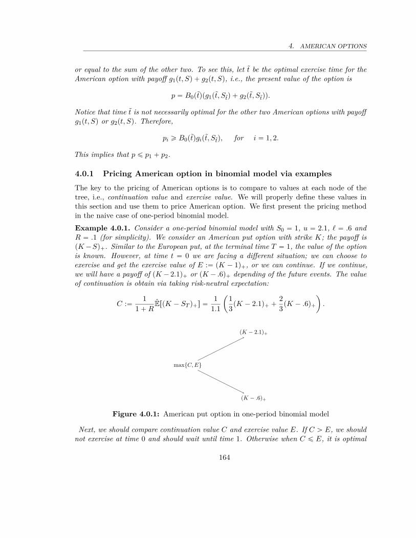
4. AMERICAN OPTIONS
or equal to the sum of the other two. To see this, let t be the optimal exercise time for theAmerican option with payoff g1pt, Sq ` g2pt, Sq, i.e., the present value of the option is
p “ B0ptqpg1pt, Stq ` g2pt, Stqq.
Notice that time t is not necessarily optimal for the other two American options with payoffg1pt, Sq or g2pt, Sq. Therefore,
pi ě B0ptqgipt, Stq, for i “ 1, 2.
This implies that p ď p1 ` p2.
4.0.1 Pricing American option in binomial model via examples
The key to the pricing of American options is to compare to values at each node of thetree, i.e., continuation value and exercise value. We will properly define these values inthis section and use them to price American option. We first present the pricing methodin the naive case of one-period binomial model.Example 4.0.1. Consider a one-period binomial model with S0 “ 1, u “ 2.1, ℓ “ .6 andR “ .1 (for simplicity). We consider an American put option with strike K; the payoff ispK ´Sq`. Similar to the European put, at the terminal time T “ 1, the value of the optionis known. However, at time t “ 0 we are facing a different situation; we can choose toexercise and get the exercise value of E :“ pK ´ 1q`, or we can continue. If we continue,we will have a payoff of pK ´ 2.1q` or pK ´ .6q` depending of the future events. The valueof continuation is obtain via taking risk-neutral expectation:
C :“ 11 ` R
ErpK ´ ST q`s “1
1.1
ˆ
13
pK ´ 2.1q` `23
pK ´ .6q`
˙
.
maxC,E
(K − 2.1)+
(K − .6)+
Figure 4.0.1: American put option in one-period binomial model
Next, we should compare continuation value C and exercise value E. If C ą E, we shouldnot exercise at time 0 and should wait until time 1. Otherwise when C ď E, it is optimal
164
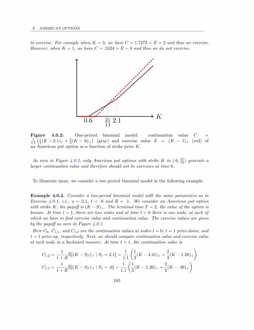
4. AMERICAN OPTIONS
to exercise. For example when K “ 3, we have C “ 1.7273 ă E “ 2 and thus we exercise.However, when K “ 1, we have C “ .2424 ą E “ 0 and thus we do not exercise.
0.6 2.1K
2113
Figure 4.0.2: One-period binomial model: continuation value C “1
1.1`1
3pK ´ 2.1q` ` 23pK ´ .6q`
˘
(gray) and exercise value E “ pK ´ 1q` (red) ofan American put option as a function of strike price K.
As seen in Figure 4.0.2, only American put options with strike K in p.6, 2113q generate a
larger continuation value and therefore should not be exercises at time 0.
To illustrate more, we consider a two period binomial model in the following example.
Example 4.0.2. Consider a two-period binomial model with the same parameters as inExercise 4.0.1, i.e., u “ 2.1, ℓ “ .6 and R “ .1. We consider an American put optionwith strike K; the payoff is pK ´ Sq`. The terminal time T “ 2, the value of the option isknown. At time t “ 1, there are two nodes and at time t “ 0 there is one node, at each ofwhich we have to find exercise value and continuation value. The exercise values are givenby the payoff as seen in Figure 4.0.3Here C0, C1,1, and C1,2 are the continuation values at nodes t “ 0, t “ 1 price-down, and
t “ 1 price-up, respectively. Next, we should compare continuation value and exercise valueat each node in a backward manner. At time t “ 1, the continuation value is
C1,2 “1
1 ` RErpK ´ ST q` | S1 “ 2.1s “
11.1
ˆ
13
pK ´ 4.41q` `23
pK ´ 1.26q`
˙
C1,1 “1
1 ` RErpK ´ ST q` | S1 “ .6s “
11.1
ˆ
13
pK ´ 1.26q` `23
pK ´ .36q`
˙
165
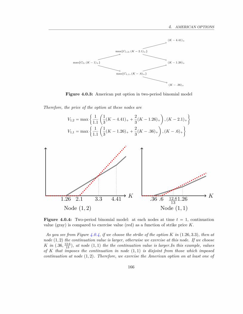
4. AMERICAN OPTIONS
maxC0, (K − 1)+
maxC1,2, (K − 2.1)+
maxC1,1, (K − .6)+
(K − 1.26)+
(K − 4.41)+
(K − .36)+
Figure 4.0.3: American put option in two-period binomial model
Therefore, the price of the option at these nodes are
V1,2 “ max"
11.1
ˆ
13
pK ´ 4.41q` `23
pK ´ 1.26q`
˙
, pK ´ 2.1q`
*
V1,1 “ max"
11.1
ˆ
13
pK ´ 1.26q` `23
pK ´ .36q`
˙
, pK ´ .6q`
*
1.26 2.1 4.413.3K
Node (1, 2)
.36 .6 1.2612.613
Node (1, 1)
K
Figure 4.0.4: Two-period binomial model: at each nodes at time t “ 1, continuationvalue (gray) is compared to exercise value (red) as a function of strike price K.
As you see from Figure 4.0.4, if we choose the strike of the option K in p1.26, 3.3q, then atnode p1, 2q the continuation value is larger, otherwise we exercise at this node. If we chooseK in p.36, 12.6
13 q, at node p1, 1q the the continuation value is larger.In this example, valuesof K that imposes the continuation in node p1, 1q is disjoint from those which imposedcontinuation at node p1, 2q. Therefore, we exercise the American option on at least one of
166

4. AMERICAN OPTIONS
these nodes.Now let fix our put option by choosing K “ 2. Then, we continue at node p1, 2q and
exercise at node p1, 1q. Therefore, at time t “ 1, the option takes values
V1,2 “ C1,2 « 0.4485 and V1,1 “ 1.4.
At time t “ 0, we need to see if it is optimal to exercise or if it is optimal to continue. Thesituation at node p0, 0q is explained in Figure 4.0.5. The exercise value is E “ 1 but thecontinuation value is positive, i.e., C “ .9844. Therefore, it is optimal to exercise.
maxC,E = E = 1
0.4485
1.4000
Figure 4.0.5: American put option at time t “ 0 in two-period binomial model of Example4.0.2.
Remark 4.0.4. As a general rule, when it is optimal to exercise, i.e., the continuationvalue is less than or equal to exercise value, there is no point in continuing the option. Thisis because the continuation value remains equal to exercise value since then after. This canbe observed from Example 4.0.2 by taking for example K “ 1. The schematic pattern ofexercise and continuation nodes is presented in Figure 4.0.6.
(1,.2424)
(2.1,0)
(.6,.4)
(4.41,0)
(1.26,0)
(.36,.46)K = 1
(1,1)
(2.1,.9)
(.6,1.4)
(4.41,0)
(1.26,.74)
(.36,1.64)K = 2
Figure 4.0.6: The pattern of continuation versus exercise in a two-period binomial modelin Example 4.0.2. The red nodes are the exercise nodes and blue nodes are continuationnodes. In the pair pa, bq, a is the asset price and b is the continuation value.
Exercise 4.0.1. In Example 4.0.2, take the following values of K.
167
4.1. PRICING AMERICAN OPTION IN BINOMIAL MODEL; PROBLEMFORMULATION 4. AMERICAN OPTIONS
a) K “ 1.
b) K “ 3.
4.1 Pricing American option in binomial model; problemformulation
In this section, we formulate the problem of pricing an American option with (nonnegative)payoff gpt, Sq in T -period binomial model. Notice that to price an American option, it isimportant to know the best exercise time for the holder of the option. Since the price of theunderlying is randomly changing over time, the best execution time can also be a randomtime. To formulate an exercise strategy as a random time, we need to define the notion ofstopping time. Recalling from Definition B.16, we define an exercise strategy for the multiperiod binomial model.
Definition 4.1.1. An exercise strategy for an American option is a stopping time withrespect to price of underlying tSt : t “ 0, ...u, i.e., is a random variables τ : Ω Ñ t0, ..., T u
such that for any t “ 0, ..., T , the even τ ď t is known given the values of Su for u ď t.
In other words, exercise strategy is a stopping time with respect to the information gen-erated by the price process. Given the holder of an American option chooses a specificstopping time τ , the corresponding value of the option is obtained through
E” 1
p1 ` Rqτgpτ, Sτ q
ı
.
Therefore, the (optimal) value of the option for the holder is given by the maximum valueover all exercise strategies;
V0 :“ maxτPT0
E” 1
p1 ` Rqτgpτ, Sτ q
ı
,
where the maximum is taken over the set T0 all stopping times τ with values in t0, ..., T u.Since the binomial model can be constructed on a finite sample space (the set of all priceprocess paths is finite), then the set T0 is finite and therefore in the above e can show thevalue of the American option with a maximum. More generally, given the option has notbeen exercised until time t, then the value of the option is given
Vt :“ maxτPTt
Er1
p1 ` Rqτ´tgpτ, Sτ q | Fts. (4.1.1)
Here the maximum is taken over the finite set Tt of all stopping times τ with values intt, ..., T u. Since T0 is finite, there exists an optimal exercise strategy (stopping time) ϱ˚
168

4. AMERICAN OPTIONS 4.1. AMERICAN OPTION IN BINOMIAL MODEL
with values in t0, ..., T u such that
V0 “ E” 1
p1 ` Rqϱ˚ gpϱ˚, Sϱ˚q
ı
Similarly at time t, there exists an optimal a stopping time ϱ˚t with values in tt, ..., T u such
thatVt “ E
” 1p1 ` Rqϱ˚
t ´tgpϱ˚
t , Sϱ˚t
q | Ft
ı
We explain the methodology for pricing American option in the simple one-period caseby choosing t “ T ´ 1, i.e.
VT ´1 :“ maxτPTT ´1
Er1
p1 ` Rqτ´T `1 gpτ, Sτ q | FT ´1s,
where the maximum is taken over all stopping times τ with two values T ´ 1 and T ; theformer corresponds to decision to exercise at time T ´ 1, while the latter is to continueuntill maturity T . Given FT ´1, for any stopping time τ with two values tT ´ 1, T u, theevents tτ “ T ´ 1u “ tτ ď T ´ 1u and tτ “ T u “ tτ ď T ´ 1uA are both known. Therefore,either τ “ T ´ 1 a.s. or τ “ T a.s.. When τ “ T ´ 1 we obtain the exercise valuegpT ´ 1, ST ´1q; otherwise τ “ T yields the continuation value 1
1`R ErgpT, ST q | FT ´1s.Therefore, the choice of exercise strategy boils down to choosing the maximum of theexercise value gpT ´ 1, ST ´1q and the continuation value 1
1`R ErgpT, ST q | FT ´1s, i.e.
VT ´1 “ max! 1
1 ` RErgpT, ST q | FT ´1s, gpT ´ 1, ST ´1q
)
.
By using the Markov property of the binomial model, we have ErgpT, ST q | FT ´1s “
ErgpT, ST q | ST ´1s and thus the value of the American option is a function of time T ´ 1and asset price ST ´1, i.e.
V pT ´ 1, ST ´1q “ max! 1
1 ` RErgpT, ST q | ST ´1s, gpT ´ 1, ST ´1q
)
.
In this one period situation, it is not hard to see that the optimal stopping time is obtainedby the first time t (among T ´ 1, and T ) that the exercise value gpt, Stq is not smaller thancontinuation value 1
1`R ErgpT, ST q | ST ´1s. Notice that from Remark 4.0.2 the value of theAmerican option at maturity time T is always equal gpT, ST q and
V pT ´ 1, ST ´1q “ max! 1
1 ` RErVT | ST ´1s, gpT ´ 1, ST ´1q
)
.
In the sequel, we would like to extend the above implication to all t. More precisely, weseek to show the following theorem.
169
4.1. AMERICAN OPTION IN BINOMIAL MODEL 4. AMERICAN OPTIONS
Theorem 4.1.1. The value of the American option with payoff function gpt, Sq is a func-tion V pt, Sq of time t and the asset price S which satisfies
V pt, Stq “ max! 1
1 ` RErV pt ` 1, St`1q | Sts, gpt, Stq
)
(4.1.2)
Here the supremum is over all stopping times with values in tt, ..., T u. In addition, we showthat an optimal exercise strategy is given by the stopping time τ˚
t defined by the first timeu ě t such that V pu, Suq “ gpu, Suq, i.e.,
τ˚t “ inftu : u “ t, ..., T, such that V pu, Suq “ gpu, Suqu. (4.1.3)
Recall that from Remark 4.0.1, we already know that Vt ě gpt, Stq. Therefore (4.1.3)representation for an optimal exercise implies that V pt, Stq ą gpt, Stq if and only if τ˚
t ą t.To prove Theorem 4.1.1, we define a new process V by
#
VT :“ gpT, ST q
Vt :“ max 1
1`R ErVt`1 | Fts, gpt, Stq(
t “ 0, ..., T ´ 1. (4.1.4)
The following lemma presents some key properties for the study of an American option.
Lemma 4.1.1. The following properties hold for Vt and Vt defined by 4.1.1 and 4.1.4,respectively.
i) Both Vtp1`Rqt and Vt
p1`Rqt are supermartingales with respect to filtration generated bythe asset price.
ii) Vt and Vt are greater than or equal to gpt, Stq.
iii) Vt is the smallest process with property (i) and (ii).
iv)! V
u^τ˚t
p1`Rqu^τ˚
t: u “ t, ..., T
)
is a martingale.
Property (i) asserts that the discounted price of an American option is a supermartingaleand property (ii) simply restates that the value of the American option is never smallerthan the payoff. Property (iii), which is a crucial property of the value of American option,indicates that the discounted values of the American option is the smallest supermartingalewhich is greater than or equal to the discounted payoff.
Proof of Lemma 4.1.1. Given Ft, for any stopping time τ with values in tt, ..., T u, theoccurrence of the event tτ ď tu “ tτ “ tu is known. Therefore,
• If τ “ t has happened then strategy τ suggests to exercise and
E” 1
p1 ` Rqτ´tgpτ, Sτ q | Ft
ı
“ gpt, Stq.
170
4. AMERICAN OPTIONS 4.1. AMERICAN OPTION IN BINOMIAL MODEL
• If τ “ t has not happened, then strategy τ suggests to continue.
Therefore,
Vt “ maxτPTt
Er1
p1 ` Rqτ´tgpτ, Sτ q | Fts “ max
maxτPTt`1
Er1
p1 ` Rqτ´tgpτ, Sτ q | Fts, gpt, Stq
(
(4.1.5)
ě1
1 ` Rmax
τPTt`1Er
1p1 ` Rqτ´t´1 gpτ, Sτ q | Fts.
Let ϱ˚t`1 be an optimal exercise for Vt`1, i.e.
Vt`1 “ E” 1
p1 ` Rqϱ˚t`1´t´1 gpϱ˚
t`1, Sϱ˚t`1
q
ı
.
Then, in particular we have
Vt ě Er1
p1 ` Rqϱ˚t`1´t
gpϱ˚t`1, Sϱ˚
t`1q | Fts “
11 ` R
ErVt`1 | Fts.
Therefore, Vtp1`Rqt is a supermartingale. The supermartingale property for Vt
p1`Rqt is a directconsequence of its definition (4.1.4), i.e.
Vt “ max 1
1 ` RErVt`1 | Fts, gpt, Stq
(
ě1
1 ` RErVt`1 | Fts.
Hence, (i) is proven. (ii) is a straightforward consequence of choosing τ ” t in (4.1.1) and(4.1.4).
To show (iii), let Yt be another process which satisfies (i)-(ii). In particular, YT ě
gpT, ST q “ VT . Inductively, assume that Yu ě Vu for u ą t. If Vt “ gpt, Stq, thenproperty (ii) for Yt implies Vt “ gpt, Stq ď Yt. Otherwise, Vt ą gpt, Stq and we deduce from(4.1.5) that
Vt “ maxτPTt`1
Er1
p1 ` Rqτ´tgpτ, Sτ q | Fts.
Since Yt satisfies (ii), we have
Vt ď maxτPTt`1
Er1
p1 ` Rqτ´tYτ | Fts.
By optional sampling theorem, Theorem B.6, we obtain
Er1
p1 ` Rqτ´tYτ | Fts ď Yt.
171

4.1. AMERICAN OPTION IN BINOMIAL MODEL 4. AMERICAN OPTIONS
Hence, Vt ď Yt.
Remark 4.1.1 (Snell envelope). For any given payoff process g :“ tgtutě0, for instancegt “
gpt,Sq
p1`Rqt , the smallest supermartingale which is greater than or equal to g is called Snellenvelope of g. Therefore, the discounted value of the American option is the Snell envelopeof the discounted payoff.
First, we use the properties (i)-(iii) in Lemma 4.1.1 to show that Vt “ Vt for all t.
Lemma 4.1.2. For any t “ 0, ..., T , we have Vt “ Vt.
Proof. Obviously, VT “ gpT, ST q “ VT . If Vt`1 “ Vt`1, then
Vt “ max! 1
1 ` RErVt`1 | Fts, gpt, Stq
)
“ max! 1
1 ` RErVt`1 | Fts, gpt, Stq
)
.
By (i) (supermartingale property of discounted V ) and (ii), we have
Vt ď max
Vt, gpt, Stq(
“ Vt.
On the other hand, since Vt is the smallest process with properties (i) and (ii), we musthave Vt ď Vt, which verifies the equality.
Next lemma is on the Markovian property of the price of American option.
Lemma 4.1.3. The value of the American option Vt is a function of time t and asset priceS, i.e., Vt “ V pt, Stq.
Proof. If Vt`1 “ V pt ` 1, St`1q, then by Markovian property of binomial model, we obtainErV pt ` 1, St`1q | Fts “ ErV pt ` 1, St`1q | Sts and
Vt “ max! 1
1 ` RErV pt ` 1, St`1q | Sts, gpt, Stq
)
is a function V pt, Stq of time and the asset price. Hence, (4.1.2) follows.
Finally, we show that (4.1.3) provides an optimal exercise.
Lemma 4.1.4. The stopping time τ˚t given by 4.1.3 satisfies
Vt “ E” 1
p1 ` Rqτ˚t ´t
gpτ˚t , Sτ˚
tq | Ft
ı
Proof. Notice that by definition, Vτ˚t
“ gpτ˚t , Sτ˚
tq. Hence, by the optional sampling theo-
rem, Theorem (B.6), and property (iv), we obtain that
Vt “ Vt^τ˚t
“ E” 1
p1 ` Rqτ˚t ´t
V pτ˚t , Sτ˚
tq | Ft
ı
“ E” 1
p1 ` Rqτ˚t ´t
gpτ˚t , Sτ˚q | Ft
ı
,
172

4. AMERICAN OPTIONS 4.1. AMERICAN OPTION IN BINOMIAL MODEL
which shows that τ˚t is optimal.
The above discussion suggests the following algorithm in pricing American options.
Pricing American options in binomial model1: At time T , the value of the option is gpT, ST pjqq.2: for each t “ T ´ 1, ..., 0 do3: for each j “ 1, ..., t ` 1 do4: Exercise value = gpt, Stpjqq.5: Continuation value = 1
1`R ErV pt ` 1, St`1q | St “ Stpiqs “ 11`R
`
V i`1t`1 πu ` V i
t`1πℓ
˘
.6: The value of the option V pt, Stpiqq “ max
!
gpt, Stpiqq, 11`R ErV pt ` 1, St`1q | St “ Stpiqs
)
.7: If V pt, Stpiqq “ gpt, Stpiqq, we exercise the option and stop.8: If V pt, Stpiqq ą gpt, Stpiqq, we continue and the replicating portfolio is given by
∆tpStpjqq units of risky assets and V pt, Stpiqq ´ ∆tpStpjqqStpjq is cash.9: end for
10: end for
Remark 4.1.2 (Path dependent American option). If the payoff of the American optiondepends on the path, one can adjust the algorithm by considering the path dependent con-tinuation value and path dependent exercise value. Exercise 4.1.1 provides an example ofsuch kind.
Example 4.1.1 (American call option on a nondividend asset does not exist!). In thiscase the payoff is given by gpt, Sq “ pS ´ Kq`. Then, the price of the American call optionis the same as the price of European call option! In fact, this is true in any model wherethe pricing of European claims is carried by the risk-neutral probability. See Proposition4.1.1.
This situation is not unique to American call option. The following proposition furtherelaborate on this matter.
Proposition 4.1.1. Consider an American option with a convex payoff gpSq such thatgp0q “ 0 on an asset which pays no dividend. Assume that the price of a European contin-gent claim is given by
V Eupt, Sq “ BtpT qErgpST q | St “ Ss,
where E is expectation under risk-neutral probability, and the discounted asset price St “St
p1`Rqt is a martingale under risk-neutral probability. Then, the price of American optionV Ampt, Sq with payoff gpSq is the same as V Eu, i.e.
V Eupt, Sq “ V Ampt, Sq.
173

4.1. AMERICAN OPTION IN BINOMIAL MODEL 4. AMERICAN OPTIONS
Remark 4.1.3. Proposition 4.1.1 is only true when the underlying asset does not paydividend. See Exercise 4.1.2.
Exercise 4.1.1. Consider a two-period binomial model for a risky asset with each periodequal to a year and take S0 “ $1, u “ 1.5 and ℓ “ 0.6. The interest rate for both periods isR “ .1.
a) Price an American put option with strike K “ .8.
b) Price an American call option with strike K “ .8.
c) Price an American option with a path dependent payoff which pays the running max-imum1 of the path.
Remark 4.1.4. A naive example of an American option is the case where the payoff is $1.In this case, if the interest rate is positive, it is optimal to exercise the option right away.However, if interest rate is 0, the time of exercise can be any time. This naive example hasan important implication. If interest rate is zero, one can remove condition gp0q “ 0 fromProposition 4.1.1, simply by replacing payoff g by gpSq “ gpSq ´ gp0q. Since cash value ofgp0q does not change value over time, the value of the American option with payoff gpSq isgp0q plus the value of American option with payoff gpSq.For negative interest rate, the exercise date will be postponed compared to the positiveinterest rate.For example, if the interest rate is zero, the price of American put is equal to the price ofEuropean put.
Hedging American option in binomial model
Hedging American option in binomial model follows the same way as European option.The only difference is that the hedging may not continue until maturity because of theearly exercise. Given that we know the price V pt ` 1, St`1piqq of the American option attime t ` 1 at all states i “ 1, ..., t ` 2, to hedge at time t and state j, we need to keep∆tpStpjqq units of risky asset in the replicating portfolio and V pt, Stpiqq ´ ∆tpStpjqqStpjq
in cash, where ∆tpSq is given by (2.2.4), i.e.
∆pt, Sq :“ V pt ` 1, Suq ´ V pt ` 1, Sℓq
Spu ´ ℓqfor t ă τ˚.
Notice that hedging an American contingent claim is only matters before the time of theexercise. At the time of the exercise or thereafter, there is no need to hedge. However, ifthe holder of the American claim decides not to exercise at time τ˚, the issuer can continuehedging with no hassle. For example, in Example 4.0.2 with K “ 2, it is optimal for the
1The running maximum at time t is the maximum of the price until or at time t.
174

4. AMERICAN OPTIONS4.2. PRICING AMERICAN OPTION IN BLACK-SCHOLES MODEL
holder to exercise the option at the beginning, where the price of asset is $ 1. Therefore,the issuer need $ 1 to replicate. However, if the holder continues, the replication problemin the next period leads to solving the following system of equation.
#
2.1a ` 1.1b “ .4485.6a ` 1.1b “ 1.4000
which yields a “ ´1.903 and b “ 2.3107. Therefore, the issuer needs $ a ` b “ .4077 toreplicate the option which is less than $ 1 if the holder exercises the option.
Exercise 4.1.2. Consider a two-period binomial model for a risky asset with each periodequal to a year and take S0 “ $1, u “ 1.2 and ℓ “ 0.8. The interest rate for both periods isR “ .05.
a) If the asset pays 10% divided yield in the first period and 5% in the second period,find the price of an American and European call options with strike K “ .8.
b) Construct the replicating portfolio for both American and European call option.
4.2 Pricing American option in Black-Scholes model
In continuous time, including Black-Scholes model, the definition of exercise policy (stop-ping time) for American options is not easy to define. The definition needs to use filtrationand σ-algebra from measure theory2. Here we avoid technical discussion of stopping timesand only present the solution for American option in Black-Scholes model.First notice that Proposition 4.1.1 implies that the American call option is Black-Scholes
model has the same price as European call if the underlying does not pay any dividend.Therefore, our focus here is on the derivatives such as American put or American call ona dividend paying asset.The key to solve the American option problem in Black-Scholes model is to set up a free
boundary problem. This type of problems are widely studied in physics. For example, inorder to understand how an ice cube is melting over time, we need to solve a free boundaryproblem. Or if we push an elastic object to a certain shape, after releasing, the shape startschanging in a certain way which can be realized by solving a free boundary problem. SeeFigure 4.2.1.Another simple example occurs if we add obstacle underneath a hanging elastic rubber.
An elastic rubber fixed at two level points takes shape as a piece of parabola shown in leftimage in Figure 4.2.2. The equation satisfied by the free rubber is u2 “ c where the constantc depends on the physical properties of the rubber. If we position an obstacle underneaththe rubber such that the elastic rubber is touched, then it changes the shape of the red
2For more information see for example [26, 35] or for a more advanced text see [20, Chapter 1].
175
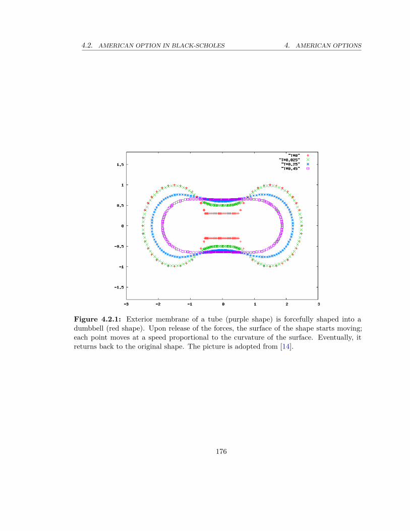
4.2. AMERICAN OPTION IN BLACK-SCHOLES 4. AMERICAN OPTIONS
Figure 4.2.1: Exterior membrane of a tube (purple shape) is forcefully shaped into adumbbell (red shape). Upon release of the forces, the surface of the shape starts moving;each point moves at a speed proportional to the curvature of the surface. Eventually, itreturns back to the original shape. The picture is adopted from [14].
176

4. AMERICAN OPTIONS 4.2. AMERICAN OPTION IN BLACK-SCHOLES
curve shown in right image in Figure 4.2.2. The position of the red curve satisfies thesame equation u2 “ c but only at the points where the rubber in not touching the obstacle.Inside the touching region px0, x1q, the rubber takes the shape of the obstacle. At the twoendpoints of touching region, the shape of the rubber is once continuously differentiable;i.e., if the upx0q “ upx1q “ y0 the height of the obstacle and u1px0q “ u1px1q “ 0.
x0 x0 x1
y0
Figure 4.2.2: The blue curve on the left shows the position of a free elastic hanging attwo points. The red curve shows the same elastic rubber hanging at the same points butbounded below by an obstacle.
After this short introduction, we come back to the problem of pricing and hedging Ameri-can option. For the sake of simplicity, we only consider simple case where there is only onefree boundary. This for example occurs when we have an American put or an Americancall on a dividend paying asset. Below, we list the important facts that you need to knowabout the free boundary.
a) The domain for the problem tpt, Sq : t P r0, T s, and S P r0, 8qu is divided into toparts separated by a curve C :“ tpt, S˚ptqq : t P r0, T su. The curve C is called freeboundary.
b) On one side of the boundary it is not optimal to exercise the option. This side iscalled continuation region, e.g. if the asset price Ss ą S˚psq for all s ď t, it has neverbeen optimal to exercise the option before or at time t.
c) The other side of the boundary is called exercise region, e.g. if the asset price St ď
S˚ptq, then it is optimal to exercise the option at time t. Therefore, the optimalstopping time is the first time that the pair pt, Stq hits the exercise region. Moreprecisely, the asset price St hits the free boundary at time t at point S˚ptq.
τ˚ :“ inf tt ď T : St “ S˚ptqu .
177

4.2. AMERICAN OPTION IN BLACK-SCHOLES 4. AMERICAN OPTIONS
It is important to notice that the exercise boundary is an unknown in pricing Americanoptions in continuous time. The other unknown is the price of the American option. Wenext explain that finding the price of the American option also gives us the the free bound-ary. The relation between these two is lied in the following representation of the stoppingpolicy. For an American option with payoff gpt, Stq, we have the optimal stopping τ˚ givenby
τ˚ “ inf tt ď T : V pt, Stq “ gpt, Stqu .
See [27] for more details. Therefore, finding the price of American option is the first priorityhere, which will be explained in the sequel.
Finding the edges of exercise boundary
So far, we learned that the domain of the problem is split into continuation boundary andexercise boundary; e.g. for American put at each time t, p0, S˚ptqq is the interior of exerciseregion and pS˚ptq, 8q is the interior of the continuation region. determining continuationregion is the matter of guess-and-check; we must look at the payoff of the American optionto guess the topology of the continuation region. One general rule is that it is notoptimal to exercise in the out of money region or where the payoff takes itsminimum value. We consider the following examples to clarify this rule:
a) American put. An American put option with strike K is out-of-money if St ą
K, and since it is not optimal to exercise in the out-of-money region, the exerciseboundary should be inside the in-the-money region, i.e., S˚ptq ď K. See Figure 4.2.3on the left. At the maturity (t “ T ), S˚pT q “ K.
b) American call. An American call option with strike K on a dividend paying assetis out-of-money if St ă K, and since it is not optimal to exercise in the out-of-money region, the exercise boundary should be inside the in-the-money region, i.e.,S˚ptq ě K. See Figure 4.2.3 on the left. At the maturity (t “ T ), S˚pT q “ K.
c) Straddle. Several other options including strangle, bull and bear spread, etc can alsobe argued in the similar fashion. However, we only explain it for straddle. First noticethat one can shift the payoff of a straddle option by cash amount of K
2 so that the newpayoff is positive. The key to analyze the straddle is that it is the least desirable toexercise the option at and around the minimum point. Therefore, we can guess thatthere are two free boundaries, S˚
1 ptq and S˚2 ptq , located symmetrically on two sides of
the minimum point of the payoff K. At the maturity (t “ T ), S˚1 pT q “ S˚2pT q “ K;
the free boundaries collapse to K.
The position of the free boundary with respect time in the three examples is sketched inFigure 4.2.5.
178

4. AMERICAN OPTIONS 4.2. AMERICAN OPTION IN BLACK-SCHOLES
K K
St St
S∗(t) S∗(t)
Figure 4.2.3: Left: Free boundary of American put at time t. Right: Free boundary ofAmerican call (on dividend paying asset) at time t. The continuation region in markedwith |—|.
K
K2
St
g(St)
S∗1(t) S∗
2(t)
K
K2
St
g(St)
S∗1(t) S∗
2(t)
Figure 4.2.4: Two free boundaries of straddle.The continuation region in marked with|—|. The free boundaries can occur both on the positive regions of the payoff and onthe negative region of the payoff. If the time-to-maturity is long, we guess that the freeboundaries are wides apart and as time-to-maturity decreases, they get closer.
Remark 4.2.1. The price of an American option with payoff equal to g1pSq ` g2pSq isnot equal to, but only smaller than, the summation of prices of an American option withpayoff g1pSq and an American option with payoff g2pSq Similar phenomenon is observedin Exercise 1.2.3.
Smooth fit
The main tool in finding the free boundary and to evaluate American options in the prin-ciple of smooth fit.Let’s denote the price of the American option at time t when the asset price is equal to
St “ S by V pt, Sq. We provide the methodology for American put option. For other cases,the method can be adopted after necessary modifications. Before presenting this principle,we shall explain that in the continuation region, the price function V pt, Sq of the American
179

4.2. AMERICAN OPTION IN BLACK-SCHOLES 4. AMERICAN OPTIONS
0 0.2 0.4 0.6 0.8 11
1.2
1.4
1.6
1.8
2
Exercise region
Continuation region
0 0.2 0.4 0.6 0.8 1
2
2.2
2.4
2.6
2.8
Exercise region
Continuation region
0 0.2 0.4 0.6 0.8 11
1.5
2
2.5
Exercise region
Exercise region
Continuation region
Figure 4.2.5: Sketch of the position of American option exercise boundary in time (hor-izontal axis). Left: American put. Middle: American call (dividend). Right: AmericanStraddle.
put option satisfies Black-Scholes equation, i.e.$
’
&
’
%
BtV pt, Sq ` σ2S2
2 BSSV pt, Sq ` rSBSV pt, Sq ´ rV pt, Sq “ 0 for S ą S˚ptq
V pt, Sq “ gpt, Sq for S ď S˚ptq
V pT, Sq “ gpT, Sq;. (4.2.1)
Therefore, S˚ptq serves as a boundary for the above equation. However, S˚ptq itself is anunknown. With the Black-Scholes equation, we have two unknowns but only one equation.Principal of smooth fit provides a second equation.
Proposition 4.2.1 (Principal of smooth fit). Assume that the payoff gpt, Sq of the Ameri-can option is twice continuously differentiable with respect to S and continuous in t. Then,at the free boundary S˚ptq, we have
V pt, S˚ptqq “ gpt, S˚ptqq, and BSV pt, S˚ptqq “ BSgpt, S˚ptqq,
for all t ă T .
For example for American put we have gpt, Sq “ pK ´Sq`. Therefore, principle of smoothfit implies that V pt, S˚ptqq “ pK ´ S˚ptqq` and BSV pt, S˚ptqq “ ´1.To see how smooth fit can be used in pricing American options, we provide some exactly
solvable example in the following. These examples are called perpetual American optionswith maturity T “ 8. As a result, the price of the American option does not dependon time and the term BtV in PDE (4.2.1) vanishes. Therefore, the pricing function V pSq
satisfies the ODEσ2S2
2V 2pSq ` rSV 1pSq ´ rV pSq “ 0,
in the continuation region.
180

4. AMERICAN OPTIONS 4.2. AMERICAN OPTION IN BLACK-SCHOLES
Example 4.2.1 (Perpetual American put option). A perpetual American option is anoption with maturity T “ 8. In practice, there is no perpetual option. However, if thematurity is long (10 years), then one can approximate the price with the price of a perpetualoption.
The key observation is that since the Black-Scholes model is time-homogeneous, the freeboundary of the perpetual American put option does not depend on time, i.e., S˚ptq “ S˚
for some unknown constant S˚ ă K. On the other hand, since the time horizon is infinite,the price V pt, Sq of the American put does not depend on t, i.e., BtV pt, Sq “ 0. Thus, wehave
σ2S2
2V 1pSq ` rSV 1pSq ´ rV pSq “ 0.
The general solution of the above equation is given by
V pSq “ c1S ` c2S´ 2rσ2 .
One can argue that c1 must be equal to 0. Since as S Ñ 8, the option goes deep out-of-money and becomes worthless. To find c2, we use principle of smooth fit.
c2pS˚q´ 2r
σ2 “ K ´ S˚
c2 “σ2
2rpS˚q
2rσ2 `1.
Thus, S˚ “ rK
r` σ22
and
V pSq “
$
’
&
’
%
K ´ S S ě rK
r` σ22
σ2
2r
´
rK
r` σ22
¯2rσ2 `1
S´ 2rσ2 S ă rK
r` σ22
.
Example 4.2.2 (Perpetual American call option on continuous dividend paying asset).Consider a continuous constant dividend rate q ą 0. The free boundary in this case isgiven by a constant S˚ with S˚ ą K and the price of American option satisfies
σ2S2
2V 2pSq ` pr ´ qqSV pSq ´ rV pSq “ 0.
The general solution of the above equation is given by
V pSq “ c1Sγ1 ` c2Sγ2 ,
181
4.2. AMERICAN OPTION IN BLACK-SCHOLES 4. AMERICAN OPTIONS
where γ1 and γ2 are roots of
σ2
2γ2 `
´
r ´ q ´σ2
2
¯
γ ´ r “ 0.
Notice that γ1 and γ2 have opposite sign and the positive one is strictly larger than 1. Without loss in generality, we assume that γ1 ă 0 ă 1 ă γ2.One can argue that c1 must be equal to 0. Since as S Ñ 0, the option goes deep out-of-
money and becomes worthless. To find c2, we use principle of smooth fit.
c2pS˚qγ2 “ S˚ ´ K
c2 “1
γ2pS˚qγ2´1 .
Thus, S˚ “γ2Kγ2´1 and
V pSq “
#
S ´ K S ďγ2Kγ2´1
1γ2
pS˚q1´γ2Sγ2 S ąγ2Kγ2´1
.
Exercise 4.2.1. Formulate and solve the free boundary problem for the perpetual Americanoptions with following payoffs.
a) pS ´ Kq` ` a where a ą 0.
b) pK ´ Sq` ` a where a ą 0.
c) Straddle
d) Strangle
e) Bull call spread
f) Bear call spread
American option with finite maturity
Unlike perpetual American option, when T ă 8, there is no closed-form solution for the freeboundary problem (4.2.1). Therefore, numerical methods should be used to approximatethe solution.The simplest among numerical methods is the binomial approximation. One needs to
choose large number of periods N and apply the algorithm of “Pricing American optionsin binomial model”. The parameters of the binomial model u, ℓ , and R can be chosen ac-cording to symmetric probability, subjective return, or any other binomial which convergesto the specific Black-Scholes model.
182

4. AMERICAN OPTIONS 4.2. AMERICAN OPTION IN BLACK-SCHOLES
The finite difference scheme can be employed to solve free boundary problem numerically.Similar to Section (3.3.10), one can apply the change of variables Upτ, xq “ e´rτ V pT ´
τ, erτ`xq, to derive a heat equation with free boundary for U , i.e.$
’
&
’
%
Bτ Upτ, xq “ σ2
2 BxxUpτ, xq ` rBxV pτ, xq ´ rUpτ, xq for x ą x˚pτq
Upτ, xq “ gpT ´ τ, exq for x ď x˚pτq
Up0, xq “ gpT, exq
,
where x˚pτq “ lnpS˚pτqq.For the simplicity, we only consider American put option, where we have Upτ, xq ě gpT ´
τ, exq. Whether we want to apply explicit or implicit scheme to the above problem, becauseof the free boundary, we need to add an intermediate step between step i and step i ` 1of the scheme. Suppose that the approximate solution Upτi, xjq at τi is known for all j.Therefore, finite difference scheme (3.2.17) or (3.2.18) provides an approximate solution,denoted by Upτi` 1
2, xjq for the heat equation without including the free boundary3. Then,
to find an approximate solution Upτi`1, xjq for the free boundary problem at τi`1, one onlyneeds to set
Upτi`1, xjq :“ maxtUpτi` 12, xjq, gpT ´ τ, exj qu.
To summarize we have the following:#
Upτi` 12, ¨q :“ AUpτi, ¨q
Upτi`1, xjq :“ maxtUpτi` 12, xjq, gpT ´ τ, exj qu @j
.
Here A can be implicit, explicit or mixed scheme.The above method is in the category of splitting method, where there is one or more
intermediate steps in the numerical schemes to go from step i to step i ` 1.The splitting method described in this section can also be applied directly to Black-Scholes
equation with free boundary$
’
&
’
%
Bτ V pτ, Sq “ σ2S2
2 BSSV pτ, Sq ` rSBSV pτ, Sq ´ rV pτ, Sq for S ą S˚pτq
V pτ, Sq “ gpT ´ τ, Sq for S ď S˚pτq
V p0, Sq “ gpT, Sq;.
The CFL condition is not different in the case of free boundary problems.The Monte Carlo methods for American options are more complicated than for the Eu-
ropean options and in beyond the scope of this lecture notes. For more information of theMonte Carlo methods for American options, see [22], [8], or the textbook [17].
3The subscript in τi` 12
indicate that finite difference evaluation in each step in an intermediate step.
183

4.2. AMERICAN OPTION IN BLACK-SCHOLES 4. AMERICAN OPTIONS
American call option on discrete dividend paying asset
Unlike continuous dividend problem, the discrete dividend cannot be solved as a singlefree boundary problem. Consider an asset which pays dividend yield of d P p0, 1q at timest1 ă t2 ă ... ă tn “ T . Proposition 4.1.1 suggests that at any time t P rti, ti`1q betweenthe times of dividend payments it is better to wait and not to exercise. However, at time ti
of the dividend payment, the price of the asset decreases by the dividend and so does theprice of the call option. Therefore, if the continuation is not optimal, the option should beexercises at the moment just before the time of a dividend payment.
184

Appendices
185

A. CONVEX OPTIMIZATION
A Convex optimizationIn this section, we briefly review the important result that we need from linear and convexoptimization for this course. We start with reminding the notion of convex set and convexfunction.
A.1 Convex functions
Definition A.1. A set A Ď Rd is called convex if for any λ P p0, 1q and x, y P A, we have
λx ` p1 ´ λqy P A.
In other words, a convex set is a set which contains all the segments with endpoints insidethe set.
Example A.1. The unit disk tx P Rd : |x| ď 1u and the unit cube r0, 1sd are convexsets. The volume given by inequalities ai ¨ x ď bi for i “ 1, ..., n, ai P Rd and bi P R(enclosed within n hyperplanes) is a convex set. Euclidean space Rd and the empty set arealso convex.
Definition A.2. Let A be a convex set. A real function f : A Ď Rd Ñ R is called convexif for any λ P p0, 1q and x, y P Rd, we have
fpλx ` p1 ´ λqyq ď λfpxq ` p1 ´ λqfpyq.
A function f is called concave if ´f is convex. The convexity (concavity) is called strict ifthe inequality above is strict when x‰y.
Proposition A.1. A set A Ď Rd is called convex. Then, a function f : A Ď Rd Ñ R isconvex if and only if
f
˜
nÿ
i“1λixi
¸
ď
nÿ
i“1λifpxiq,
for all x1, ..., xn P A and λ1, ..., λn P R` withřn
i“1 λi “ 1.
If a convex function f is twice differentiable, then the Hessian matrix of second derivativesof f , ∇2f , has all eigenvalues nonnegative. In one dimensional case, this is equivalent tof2 ě 0.However, not all convex function are twice differentiable or even differentiable. We actually
know that all convex functions are continuous. In addition, we can show that the one-sideddirectional derivatives of a continuous function exits.
Proposition A.2. Let A be a convex set and f : A Ď Rd Ñ R be a convex function. Then,for all x in the interior of A and all vectors v P Rd, the directional derivative of f at x is
187

A. CONVEX OPTIMIZATION
the direction of v,
∇vfpxq :“ limεÑ0`
fpx ` εvq ´ fpxq
ε
exits and satisfies fpx ` tvq ě fpxq ` t∇vfpxq for all t ě 0. In particular, f is continuousat all points of A.In one dimensional case, for a convex functions f the above Proposition implies that the
right and left derivatives, f 1p¨`q and f 1p¨´q, exist at all points, and in particular a convexfunction is always continuous.The above proposition has an important implication about the tangent hyperplane to a
convex function.Corollary A.1. Consider a convex function f and x0 P Rd. Then, there exists someu P Rd such that the hyperplane y “ fpx0q ` px ´ x0q ¨ u always lies underneath the surface,i.e.
fpxq ě fpx0q ` px ´ x0q ¨ u for all x P Rd.
When f is differentiable, the linear approximation of f is always under-approximating thefunction, i.e.
fpxq ě fpx0q ` px ´ x0q ¨ ∇fpx0q for all v P Rd.
If a function f is twice differentiable, the Hessian ∇2f is the matrix which contains allsecond derivatives of the function f , i.e.
”
B2fBxiBxj
ı
dˆd. For twice differentiable function one
can provide a criteria for convexity based on the eigenvalues of the Hessian matrix.Corollary A.2. If all eigenvalues of the Hessian matrix ∇2f are nonnegative (positive)at all points, then the function f is convex (resp. strictly convex).One can also use the Hessian matrix to find the local minimum and maximums of a
function by checking its local convexity and concavity which is given in the following result.Recall that a point x0 for a differentiable function is called critical if ∇fpx0q “ 0.Proposition A.3. A critical point x0 for a differentiable function f is a local minimum(resp. maximum) if and only if f is convex (resp. concave) in a neighborhood of x0.
As a result of the above proposition we have the second order derivative test in multivariatecalculus.Proposition A.4. A critical point x0 for a second order differentiable function f is
i) a local minimum if the Hessian ∇2fpx0q is positive-definite.
ii) a local maximum if the Hessian ∇2fpx0q is negative-definite.
iii) a saddle point if the Hessian ∇2fpx0q has both negative and positive eigenvalues.
Exercise A.1. Find and categorize all the critical point of the function fpx, yq “ xe´x2`y2
2 .
Exercise A.2. Find and categorize all the critical point of the function fpx, yq “ xye´x2`y2
2 .
188

A. CONVEX OPTIMIZATION
A.2 Convex constrained optimization
Consider a convex function f : D Ď Rn Ñ R where the set D is given by
K “ tx P Rn : gipxq ď 0 for i “ 1, ..., mu.
We assume that all functions gi for i “ 1, ..., m are convex and therefore the set K is closedand convex. The primal problem is to minimize f in D, i.e.
min fpxq subject to constraints gipxq ď 0 for i “ 1, ..., M.
If f is strictly concave, then the optimizer is unique if it exists. Notice that the existenceof the optimizer is subject to nonemptiness of the set D.An equality constraint can also be described in the above form if the function gi is affine4
and both gipxq ď 0 and ´gipxq ď 0. For later analysis, we specify constraint equalities inthe problem separately and define the feasibility set by
K “ tx P Rn : gipxq ď 0 for i “ 1, ..., m and hjpxq “ 0 for j “, ..., ku.
Notice that since gis are convex and hjs are affine, K is convex, for any number λ P p0, 1q
and any x, y P K, λx ` p1 ´ λqy P K. Given the convex functions gi for i “ 1, ..., m andaffine functions hj for j “ 1, ..., k, the convex constrained optimization problem is given by
P :“ min fpxq subject to constraints
#
gipxq ď 0 for i “ 1, ..., m
hjpxq “ 0 for j “ 1, ..., k. (A.1)
Function f is called the objective function and the inequalities gi ď 0 and equations hj “ 0are called constraints. If K ‰ H, the problem is called feasible. if fpxq is strictly convex,then the minimizer is unique; for any two distinguished minimizers x1 and x2 with minimumvalue P “ fpx1q “ fpx2q, we have f
`
x1`x22
˘
ă 12pfpx1q ` fpx2qq “ P which contradicts
with that x1 and x2 are minimizers.Duality method is one of the useful approaches to solve the convex optimization problems.
To present the dual problem, we first introduce the Lagrangian
Lpµ, λq “ minxPRn
!
fpxq ` µ ¨ gpxq ` λ ¨ hpxq
)
.
Here µ P Rm and gpxq “ pg1pxq, ..., gmpxqqq, λ P Rk and hpxq “ ph1pxq, ..., hmpxqqq and ¨ isthe dot product in the proper Euclidean space. Then, the dual problem is given by
D :“ maxµPRm
` , λPRkLpµ, λq.
4An affine function is a linear function plus a constant; hpxq “ a ¨ x ` b, where a P Rm and b P R.
189
A. CONVEX OPTIMIZATION
Notice that for x P K, Lpµ, λq ď fpxq ` µ ¨ gpxq ` λ ¨ hpxq ď fpxq. Therefore, Lpµ, λq ď
minxPK fpxq and thus, D ď P which is called the weak duality. We can show that underthe following condition that the strong duality holds.
Assumption A.1 (Slater condition). There exist a point x0 such that gipx0q ă 0 for alli “ 1, ..., m and hjpx0q “ 0 for all j “ 1, ..., k.
Theorem A.1 (Duality). Let f , gi for i “ 1, ..., n and hj for j “ 1, ..., m are convexand Slater condition A.1 holds. Then D “ P . In addition, the dual maximizer pµ˚, λ˚q P
Rm` ˆ Rk exists whenever D ą ´8, i.e.
maxµPRm
` , λPRkLpµ, λq “ Lpµ˚, λ˚q.
A proof of this theorem can be found in [9, Section 5.3.2]. The following example showsif Slater condition fail, the strong duality does not necessarily hold.
Example A.2. Take d “ m “ 2, n “ 1 with fpx1, x2q “ x21 ` x2, g1pxq “ x2, h1pxq “
x1 ` x2 and h2pxq “ x1 ´ x2. Since feasibility set is a singleton; K “ tp0, 0qu, the Slatercondition does not hold. Therefore, P “ fp0, 0q “ 0. On the other hand, Lpµ, λq “ ´8
unless λ “ 0. Specifically, Lpµ, 0q “ minpx1,x2q fpx1, x2q ` µx2. Then, we also have
Lpµ, 0q “ minx1
x21 ` min
x2x2p1 ` µq “ ´8,
since µ ě 0. Therefore, D “ ´8 ă P “ fp0, 0q “ 0.
Remark A.1. Notice that the duality can sometimes hold when the Slater condition doesnot hold or when the problem is not even feasible. For instance, if K “ H, since minH “ 8,P “ 8. On the other hand, for and arbitrary point x0, let I and J respectively be the setof all indices i and j such that gipx0q ą 0 and hjpx0q ‰ 0. Since K “ H, at least one of Ior J is nonempty. Then, choose µ and λ such that µi “ 0 if and only if i R I and λj “ 0if and only if j R J . Therefore,
Lpµ, λq ď fpx0q ` µ ¨ gpx0q ` λ ¨ hpx0q.
By sending µi Ñ `8 for i P I and λj Ñ ˘8 whether hjpx0q is negative/positive, we obtainthat maxµPRm
` , λPRk Lpµ, λq “ `8.
One of the practical methods of finding the optimal points for primal and dual problem isthrough the KKT5, which provided a necessary condition of optimality. Additionally withSlater condition, KKT is also sufficient.
5Karush-Kuhn-Tucker
190
A. CONVEX OPTIMIZATION
Theorem A.2 (KKT optimality condition). Assume that f , g and h are differentiableand x˚ P Rd and pµ˚, λ˚q P Rm
` ˆ Rk are respectively the optimizer of the primal and dualproblems. Then,
Bxℓfpx˚q ` µ ¨ Bxℓ
gpx˚q ` λ ¨ Bxℓhpx˚q “ 0 for ℓ “ 1, ..., n
µ˚i gipx
˚q “ 0 for i “ 1, ..., m
hjpx˚q “ 0 for j “ 1, ..., k
. (A.2)
Condition µ˚i gipx
˚q “ 0 is called the complementary slackness condition. In addition, ifthe Slater condition A.1 holds and (A.2) is satisfied, then x˚ P Rd and pµ˚, λ˚q P Rm
` ˆ Rk
are respectively the the optimizer of the primal and dual problems.
Example A.3. We want to find the maximum volume of an open lid box with a fixedsurface area s by solving the constrained maximization problem
max xyz subject to constraints xy ` 2xz ` 2yz “ s.
Notice that since the Slater condition holds for x0 “ y0 “?
s and Z0 “ 0, the dual problemand primal problem have the same value. The KKT condition suggest to solve the followingto find candidates for the primal and dual problem.
xy ` 2µpx ` yq “ 0xz ` µpx ` 2zq “ 0yz ` µpy ` 2zq “ 0xy ` 2xz ` 2yz “ s
Solving the above system of equation yields
x˚ “ y˚ “ 2z˚ “
?3s
3and µ˚ “ ´
?3s
12,
and the maximum volume is s?
3s16 .
Exercise A.3. Find the volume of the largest box under the constraint that the sum of thediagonals of the three sides sharing a corner equal is to s.
The duality method, while can be used as a computational tool, it can also provide uswith some qualitative results about the optimization problem that we are studying. Forinstance, in Section 1.3.6, the dual problem for evaluation of model risk is the problem ofsuperreplication. In the next sections, we formulate the dual problem for the linear andquadratic programming.
191
A. CONVEX OPTIMIZATION
Linear programming
Linear optimization is when the objective function f and the constraints are all linear;for some constants p P Rd, ai P Rd, bi P R for i “ 1, .., m, and cj P Rd and dj P R forj “ 1, ..., k.
fpxq “ p ¨ x, gipxq “ ai ¨ x ` bi, and hjpxq “ cj ¨ x ` dj .
Therefore,
P :“ min p ¨ x subject to constraints
#
ai ¨ x ` bi ď 0 for i “ 1, ..., m
cj ¨ x ` dj “ 0 for j “ 1, ..., k. (A.3)
Let matrices A and C consist of rows a1, ..., am and c1, ..., ck, respectively and set d :“pd1, ..., dkq and b :“ pb1, ..., bmq as column vectors. Then, the linear programming can bewritten in the following compact form.
min p ¨ x subject to constraints
#
Ax ` b ď 0Cx ` d “ 0
.
Each equation cj ¨ x ` dj “ 0 is a hyperplane and each inequality ai ¨ x ` bi ď 0 is a half-space in the d-dimensional Euclidean space. The feasibility set K can easily be empty, if theconstraints are made by parallel hyperplanes; for example aix ` bi ď 0 and ai1x ` bi1 ď 0with ai “ ´ai1 and bi “ ´bi1 ´ 1. To avoid this situation, we assume that the vectorsa1, ..., am and c1, ..., ck are linearly independent in Rd. As a result, m ` k ď d the matricesA and C are full rank, where A and C are matrices with rows a1, ..., am and c1, ..., ck,respectively. In addition, we need to assume that the column vector d “ pd1, ..., dkq is inthe range of ´C and the orthant ty P Rm : y ě bi for i “ 1, ..., mu intersects with therange of ´A, Cx ` d “ 0 and Ax ` b ď 0 together have a solution for x. and are columnvectors.
The Lagrangian for the linear programming is given by
Lpµ, λq “ minxPRd
tp ¨ x ` µ ¨ pAx ` bq ` λ ¨ pCx ` dqu .
Notice that if pµ, λq are such that pT ` pµ˚qTA ` pλ˚qTC ‰ 0 then,
minxPRd
!
ppT ` µTA ` λTCq ¨ x)
` µTb ` λTd “ ´8.
Therefore,
Lpµ, λq “
#
´8 pT ` pµ˚qTA ` pλ˚qTC ‰ 0µTb ` λTd pT ` pµ˚qTA ` pλ˚qTC “ 0
.
192

A. CONVEX OPTIMIZATION
Therefore, the dual problem can be written as
D :“ maxµě0,λ
µTb ` λTd subject to constraints pT ` pµ˚qTA ` pλ˚qTC “ 0 (A.4)
Theorem A.3 (Linear programming duality). Consider the following two linear program-ming problems (A.3) and (A.4). If either of the problems has an optimal solution, so doesthe other one and both problems have the same value, D “ P .
Exercise A.4. Write the dual problem and KKT condition for the standard linear pro-gramming equation:
min p ¨ x subject to constraints
#
xi ď 0 for i “ 1, ..., d
cj ¨ x ` dj “ 0 for j “ 1, ..., k.
Exercise A.5 (Project). Study the following algorithms for the linear programming prob-lem in Exercise 1.3.10. Find a package that has both methods and compare the runningtime of each method on the same problem.
a) Simplex method
b) Interior points
Quadratic programming
Consider a positive-definite symmetric6 d-by-d matrix M , ai P Rd, bi P R for i “ 1, .., m,and cj P Rd and dj P R for j “ 1, ..., k.
fpxq “12
x ¨ Mx, gipxq “ ai ¨ x ` bi, and hjpxq “ cj ¨ x ` dj .
Therefore, the quadratic optimization problem is given by
min 12
x ¨ Mx subject to constraints
#
ai ¨ x ` bi ď 0 for i “ 1, ..., m
cj ¨ x ` dj “ 0 for j “ 1, ..., k. (A.5)
The Lagrangian for the linear programming is given by
Lpµ, λq “ minxPRd
"
12
x ¨ Mx ` µ ¨ pAx ` bq ` λ ¨ pCx ` dq
*
.
6A matrix A is symmetric if AT “ A and is positive-definite if all its eigenvalues are
193

A. CONVEX OPTIMIZATION
The dual problem for (A.5) is also a quadratic problem; the minimizer for x in the La-grangian function Lpµ, λq is given by xpµ, λq “ ´M´1pATµ ` CTλq and therefore La-grangian Lpµ, λq is a quadratic function of µ and λ. Therefore,
Lpµ, λq “ ´12
µ ¨ Aµ ` µ ¨ b ´12
λ ¨ Cλ ` λ ¨ d,
where A “ AM´1AT and C “ CM´1CT are indeed nonnegative definite symmetric matri-ces. The dual problem can now be decoupled into two problems;
maxµě0
"
´12
µ ¨ Aµ ` µ ¨ b
*
and maxλ
"
´12
λ ¨ Cλ ` λ ¨ d
*
The maximization problem on λ is an unconstrained problem which leads to λ˚ “ C´1dwhen C is invertible. The maximization problem on µ is, however, a constrained problem.One way to find the primal and the dual optimal variables X˚, µ˚ and λ˚ is through KKTcondition in Theorem (A.2), which is written as
Mx˚ ` ATµ˚ ` CTλ˚ “ 0µ˚
i paix˚ ` biq “ 0 for i “ 1, ..., m
cjx˚ ` dj “ 0 for j “ 1, ..., k
When the dual maximizer µ˚i ą 0, then by KKT condition the ith constraint must hold
with equality, aix˚ ` bi “ 0. In this case, we call the constraint an active constraint.
Exercise A.6 (Project). Study the following algorithms for the linear programming prob-lem in Section 1.1.7. Find a package that has both methods and compare the running timeof each method on the same problem.
a) Active set
b) Interior points
Computational tools for convex optimization problems
The computational methods for convex optimization problems are vast and we do notintend to study them in this book. Instead, we briefly introduce some of the tools whichyou can use to solve optimization problems in finance.A well-developed convex optimization tool is CVX under MatLab created by Michael Grant
and Stephen Boyd. The academic (noncommercial) version of the toolbox is free and undera GNU General Public License; it can be used or redistributed but not altered. However,it works under commercial software MatLab. The home of CVX is http://cvxr.com.
194
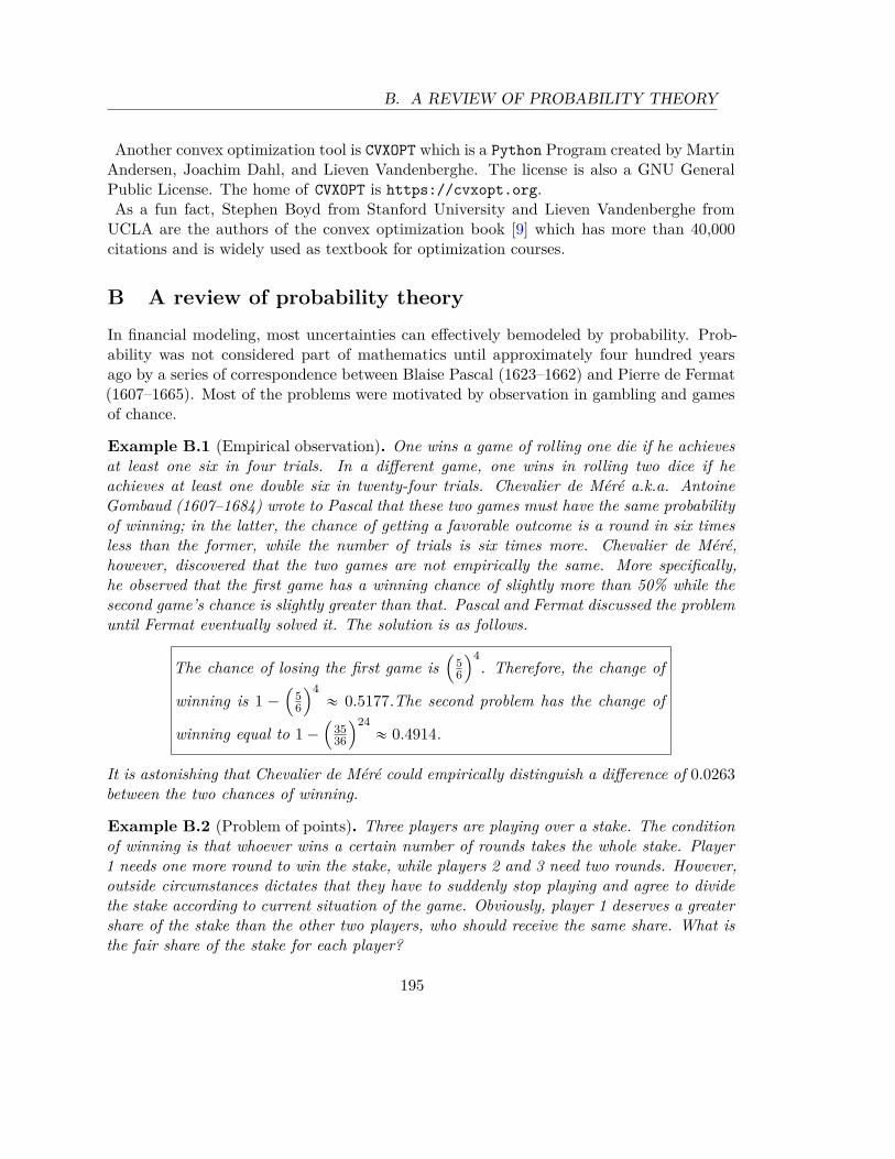
B. A REVIEW OF PROBABILITY THEORY
Another convex optimization tool is CVXOPT which is a Python Program created by MartinAndersen, Joachim Dahl, and Lieven Vandenberghe. The license is also a GNU GeneralPublic License. The home of CVXOPT is https://cvxopt.org.As a fun fact, Stephen Boyd from Stanford University and Lieven Vandenberghe from
UCLA are the authors of the convex optimization book [9] which has more than 40,000citations and is widely used as textbook for optimization courses.
B A review of probability theoryIn financial modeling, most uncertainties can effectively bemodeled by probability. Prob-ability was not considered part of mathematics until approximately four hundred yearsago by a series of correspondence between Blaise Pascal (1623–1662) and Pierre de Fermat(1607–1665). Most of the problems were motivated by observation in gambling and gamesof chance.
Example B.1 (Empirical observation). One wins a game of rolling one die if he achievesat least one six in four trials. In a different game, one wins in rolling two dice if heachieves at least one double six in twenty-four trials. Chevalier de Méré a.k.a. AntoineGombaud (1607–1684) wrote to Pascal that these two games must have the same probabilityof winning; in the latter, the chance of getting a favorable outcome is a round in six timesless than the former, while the number of trials is six times more. Chevalier de Méré,however, discovered that the two games are not empirically the same. More specifically,he observed that the first game has a winning chance of slightly more than 50% while thesecond game’s chance is slightly greater than that. Pascal and Fermat discussed the problemuntil Fermat eventually solved it. The solution is as follows.
The chance of losing the first game is´
56
¯4. Therefore, the change of
winning is 1 ´
´
56
¯4« 0.5177.The second problem has the change of
winning equal to 1 ´
´
3536
¯24« 0.4914.
It is astonishing that Chevalier de Méré could empirically distinguish a difference of 0.0263between the two chances of winning.
Example B.2 (Problem of points). Three players are playing over a stake. The conditionof winning is that whoever wins a certain number of rounds takes the whole stake. Player1 needs one more round to win the stake, while players 2 and 3 need two rounds. However,outside circumstances dictates that they have to suddenly stop playing and agree to dividethe stake according to current situation of the game. Obviously, player 1 deserves a greatershare of the stake than the other two players, who should receive the same share. What isthe fair share of the stake for each player?
195
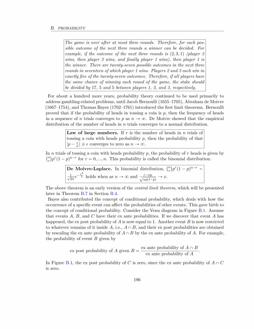
B. PROBABILITY
The game is over after at most three rounds. Therefore, for each pos-sible outcome of the next three rounds a winner can be decided. Forexample, if the outcome of the next three rounds is p2, 3, 1q (player 2wins, then player 3 wins, and finally player 1 wins), then player 1 isthe winner. There are twenty-seven possible outcomes in the next threerounds in seventeen of which player 1 wins. Players 2 and 3 each win inexactly five of the twenty-seven outcomes. Therefore, if all players havethe same chance of winning each round of the game, the stake shouldbe divided by 17, 5 and 5 between players 1, 2, and 3, respectively.
For about a hundred more years, probability theory continued to be used primarily toaddress gambling-related problems, until Jacob Bernoulli (1655–1705), Abraham de Moivre(1667–1754), and Thomas Bayes (1702–1761) introduced the first limit theorems. Bernoulliproved that if the probability of heads in tossing a coin is p, then the frequency of headsin a sequence of n trials converges to p as n Ñ 8. De Moivre showed that the empiricaldistribution of the number of heads in n trials converges to a normal distribution.
Law of large numbers. If r is the number of heads in n trials oftossing a coin with heads probability p, then the probability of that|p ´ r
n | ě ϵ converges to zero as n Ñ 8.
In n trials of tossing a coin with heads probability p, the probability of r heads is given by`
nr
˘
prp1 ´ pqn´r for r “ 0, ..., n. This probability is called the binomial distribution.
De Moivre-Laplace. In binomial distribution,`
nr
˘
prp1 ´ pqn´r „
1?2π
e´ x22 holds when as n Ñ 8 and r´np?
npp1´pqÑ x.
The above theorem is an early version of the central limit theorem, which will be presentedlater in Theorem B.7 in Section B.4.Bayes also contributed the concept of conditional probability, which deals with how the
occurrence of a specific event can affect the probabilities of other events. This gave birth tothe concept of conditional probability. Consider the Venn diagram in Figure B.1. Assumethat events A, B, and C have their ex ante probabilities. If we discover that event A hashappened, the ex post probability of A is now equal to 1. Another event B is now restrictedto whatever remains of it inside A, i.e., A X B, and their ex post probabilities are obtainedby rescaling the ex ante probability of A X B by the ex ante probability of A. For example,the probability of event B given by
ex post probability of A given B “ex ante probability of A X B
ex ante probability of A.
In Figure B.1, the ex post probability of C is zero, since the ex ante probability of A X Cis zero.
196
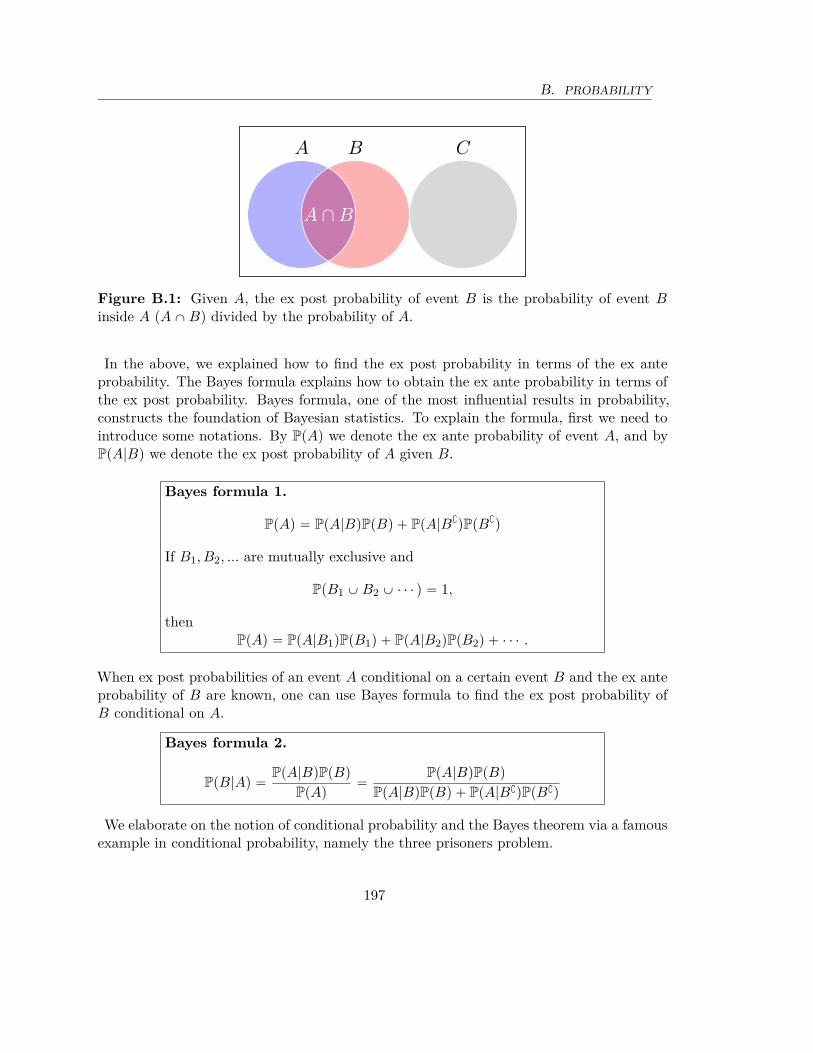
B. PROBABILITY
BA C
A ∩B
Figure B.1: Given A, the ex post probability of event B is the probability of event Binside A (A X B) divided by the probability of A.
In the above, we explained how to find the ex post probability in terms of the ex anteprobability. The Bayes formula explains how to obtain the ex ante probability in terms ofthe ex post probability. Bayes formula, one of the most influential results in probability,constructs the foundation of Bayesian statistics. To explain the formula, first we need tointroduce some notations. By PpAq we denote the ex ante probability of event A, and byPpA|Bq we denote the ex post probability of A given B.
Bayes formula 1.
PpAq “ PpA|BqPpBq ` PpA|BAqPpBAq
If B1, B2, ... are mutually exclusive and
PpB1 Y B2 Y ¨ ¨ ¨ q “ 1,
thenPpAq “ PpA|B1qPpB1q ` PpA|B2qPpB2q ` ¨ ¨ ¨ .
When ex post probabilities of an event A conditional on a certain event B and the ex anteprobability of B are known, one can use Bayes formula to find the ex post probability ofB conditional on A.
Bayes formula 2.
PpB|Aq “PpA|BqPpBq
PpAq“
PpA|BqPpBq
PpA|BqPpBq ` PpA|BAqPpBAq
We elaborate on the notion of conditional probability and the Bayes theorem via a famousexample in conditional probability, namely the three prisoners problem.
197

B. PROBABILITY
Example B.3 (Three prisoners problem). Three suspects (Bob, Kevin, and Stuart) areequally likely to be convicted. However, the judge has made up his mind and is goingto pronounce one and only one of them guilty the following morning. None of the threeprisoners knows who is going to be announced; however, the warden has been told the nameof the guilty by the judge and has been given strict orders not to pass the information tothe prisoners. Stuart argues with the warden that at least one of the other two, Kevin orBob, is not guilty. If the warden names one of the other two, Stuart still cannot knowif he himself is guilty or not. The warden counterargues that if he reveals the name of anonguilty person, Stuart’s chance of conviction increases from 1
3 to 12 , because now there
are two prisoners one of whom is going to be guilty. Is the warden correct?To answer the question, we formulate the problem using conditional probabilities. In
this case, if the warden names Bob as not guilty, then the ex ante probability of Stuart’sconviction is given by
ex ante probability of conviction of StuartŞ
Bob named not guilty by the wardenex ante probability of Bob named not guilty by the warden
.
The ex ante probability of Bob named not guilty by the warden can be calculated using theBayes formula. Let’s denote this event by B, and let S, K, and B be the events that eitherStuart, Kevin, or Bob, respectively, is announced guilty. By conditional probability, oneneeds to calculate
PpS|Bq “PpS X Bq
PpBq.
Since PpS Y K Y Bq “ 1, it follows from the first Bayes formula that
PpBq “ PpB|SqPpSq ` PpB|KqPpKq ` PpB|BqPpBq.
Notice that PpKq “ PpBq “ PpSq “ 13
7, PpB|Sq “ 12 , PpB|Kq “ 1, and PpB|Bq “ 0.
Therefore,PpBq “
16
`13
` 0 “12
.
On the other hand,PpS X Bq “ PpB|SqPpSq “
16
.
Therefore, PpS|Bq “1612
“ 13 .
In Example B.3, the revealed information does not change the ex ante probability. Thisis, however, a coincidence and not necessarily true. The following exercise addresses thisissue.
7Here we assume that they are equally likely to be pronounced guilty. One can adjust these probabilitiesand solve the problem accordingly.
198

B. PROBABILITY
Exercise B.1. Repeat the solution to Example B.3 with PpKq “ PpSq “ 16 and PpBq “ 2
3 .Beware as here is some ambiguity about how to choose PpB|Sq!
Example B.4. In a burglary hearing, there is a probability pG that the suspect is guilty.In actual fact, the suspect is left-handed. If it is brought before the court that the burglaris right-handed, the ex post probability that the suspect is guilty vanishes to zero. However,if the evidence shows that the burglar is left-handed, we need to use the Bayes formula tofind the ex post probability that the suspect is guilty. In this case, let G be the event thatthe suspect is guilty and L be the event that the burglar is left-handed that, we assume, hasthe same ex ante probability of any individual is left-handed8. Then,
PpG|Lq “PpL|GqPpGq
PpLq“
PpGq
PpLq.
Notice that PpL|Gq “ 1, because the suspect is left-handed. On the other hand,
PpLq “ PpL|GqPpGq ` PpL|GAqPpGAq “ PpGq ` PpL|GAqPpGAq
Notice that PpGq “ pG, PpGAq “ 1 ´ pG, and PpL|GAq is roughly equal to the percentage ofthe left-handed population, denoted by pL. Therefore,
PpG|Lq “pG
pG ` p1 ´ pGqpL.
Notice that when PL ă 1, then PpG|Lq ą PpGq “ pG, because pG ` p1 ´ pGqpL ă 1. Forinstance, when pL “ .1 and pG “ .15, then the ex post probability PpG|Lq is 15
23.5 . If pL “ 0,then no one in the population is left-handed except for the suspect, which makes him guilty.If pL “ 1, then everyone in the population is left-handed, PpG|Lq “ pG, and the event Ldoes not add to the information we already have.
Exercise B.2. Show that if the ex ante probability of event A is 1, then PpB|Aq “ PpBq.
The notion of conditional probability (the handling of new pieces of information in prob-ability) is one of the most influential tools in applications of probability theory. Mostimportant applications appear in Bayesian statistics, through which they contribute to allother areas of science.We conclude the discussion of early advances in probability theory by mentioning that
these early developments are gathered in Essai philosophique sur les probabilités by Pierre-Simone Laplace (1749–1827) ([21]). However, the subject still lacked mathematical rigorcompared to other areas of mathematics until a breakthrough happened in the twentiethcentury. Andrey Nikolaevich Kolmogorov (1903–1987) initiated the foundation of probabil-ity theory through measure theory, a topic in mathematical analysis. We provide a more
8It is logical to assume that the probability that a burglar is left-handed is the same as any otherindividual.
199

B. PROBABILITY
rigorous treatment of probability theory in Section B.2. In the next section, we presentthe discrete theory of probability, which does not need measure theory.
B.1 Basic concepts and definitions of discrete probability
A (finite, countably infinite) sample space is a collection of all possible outcomes of arandom experiment. Any subset A of the sample space Ω is called an event.
Example B.5 (Flipping a coin). The sample space is thead, tailu.
Example B.6 (Arrow-Debreu market model in Section 1.3). The sample space can bechosen to be t1, ..., Mu, i.e., the collection of all the possible states of the system.
Example B.7 (T -period binomial model). The sample space of the T -period binomialmodel in Section 2.2 can be chosen to be the collection of all T -sequences of the formpa1, ..., aT q where each ai is either u or ℓ. Each sample addresses the complete movementsof the asset price over time.
A probability over a finite (countably infinite) sample space Ω “ tω1, ..., ωM u (Ω “
tω1, ω2, ...u) is a vector π “ pπ1, ..., πM q (π “ pπ1, π2, ...q) of nonnegative values such thatř
ωPΩ πi “ 1. For simplicity, we write Pπpωjq “ πj if no confusion occurs. The collectionof all subsets of Ω determines the set of all events. The probability of an event A Ď Ω isthen defined by
PpAq :“ÿ
ωPA
πωi .
Evidently, P satisfies
1) PpHq “ 0,
2) PpAAq “ 1 ´ PpAq for all A Ď Ω, and,
3) If tAnuně1 is a sequence of disjoint events, then
P
˜
ď
ně1An
¸
“ÿ
ně1PpAnq.
Example B.8 (Flipping a coin). In flipping a fair coin, the probability of either heads ortails is p “ 1
2 . In flipping a unfair coin, the probability of heads is p ‰ 12 , and therefore the
probability of tails is 1 ´ p. In two consecutive flips of a fair coin, the probability of havingpH, Hq, pH, T q, pT, Hq, or pT, T q is equally 14. If the coin is not fair, then the sample spaceis not changed. But the probabilities of these outcomes change to πH “ p and πT “ 1 ´ pwhere p P r0, 1s. In two consecutive flips, we have πH,H “ p2, πH,T “ πT,H “ pp1 ´ pq, andπT,T “ p1 ´ pq2.
200

B. PROBABILITY
Example B.9 (Single asset T -period binomial model). In a binomial model with T -periods,a risk-neutral probability assigns the probability πk
uπT ´kℓ to an outcome pa1, ..., aT q in which
k of the entities are u and the T ´ k remaining are ℓ.
A random variable X is a function from sample space to Rd, X : ω P Ω ÞÑ Xpωq P Rd. Thevalues that X takes with positive probability are called the values of the random variable,x P Rd such that Ppω : Xpωq “ xq ą 0. To simplify the notation, we often write PpX “ xq
for Ppω : Xpωq “ xq. When the sample space is finite or countably infinite, the randomvariables can only take finitely of countably infinitely many values. Random variables withat most countably infinitely many values are called discrete random variables.
Remark B.1. Notice that the values of a random variable are relative to the choice ofprobability measure. For example, a random variable X : t0, 1, 2u Ñ R defined by Xpxq “ xhas values t0, 1, 2u relative to probability Pp0q “ Pp1q “ Pp2q “ 13. However, relative to anew probability Qp0q “ Qp1q “ 12 and Qp2q “ 0, the set of values is given by t0, 1u.
Example B.10. Recall from Example B.6 that the sample space for the Arrow-Debreumarket model is the set of states Ω “ t1, ..., Mu. Therefore, a random variable is given bya function X : t1, ..., Mu Ñ R. In particular, the payoff of an asset (the price of an assetat time 1 for each state of the market) in the Arrow-Debreu market model is a randomvariable. For instance, the payoff of asset i given in diagram 1.3.1 is a random variablePi,¨ : Ω Ñ R such that
Pi,¨pjq “ Pi,j .
Example B.11 (Bernoulli random variable). Flipping a coin creates a Bernoulli randomvariable by assigning values to the outcomes heads and tails. The Bernoulli random variableX takes the value 1 if the coin turns heads and 0 otherwise. If the coin has a probabilityof tails equal to p, then X “ 1 has probability p and X “ 0 has probability 1 ´ p.
Definition B.1. For an event A, the indicator of A is a random variable that takes value1 if A occurs and 0 otherwise. The indicator of A is denoted by 1A
9. The indicator randomvariable 1A is a Bernoulli random variable that takes value 1 with probability PpAq andvalue 0 with probability 1 ´ PpAq.
Example B.12 (Binomial random variable). In flipping a coin n times, the binomialrandom variable X takes the value of the number of heads. The set of values of X ist0, ..., nu. If the coin has a probability of heads equal to p, then for x in the set of values,the probability X “ x is given by
ˆ
n
x
˙
pxp1 ´ pqn´x.
9the indicator is also denoted by χA in some literature.
201
B. PROBABILITY
Example B.13 (Random walk). In a game of chance, in each round a player flips a coin.If it turns tails, he gains $1; otherwise, he loses $1. Technically, each round has an outcomegiven by 2X ´ 1 where X is a brand new Bernoulli random variable with outcomes 1 and 0.The player’s accumulated reward after two rounds is a random variable W2 that take values´2, 0, and 2 with probabilities 14, 12, and 14, respectively. If the coin has a probabilityof heads equal p, then PpW2 “ 2q “ p2, PpW2 “ ´2q “ p1´pq2, and PpW2 “ 0q “ 2p1´pqp.Here, 1 is not among the values of W2, because PpW2 “ 1q “ 0.If the player continues this game, the sequence of his accumulated wealth at all times,
W0, W1, W2, ...., is called a random walk. At time t, Wt takes values t´t, ´t ` 2, ..., tu fort “ 1, ..., T . The probability of Wt “ x is given by
ˆ
t
k
˙
pkp1 ´ pqt`1´k with k “t ` x
2.
Exercise B.3. In Example B.13, calculate PpW2 “ 2 | W1 “ 1q and PpW3 “ ´1 | W1 “ 1q.
Example B.14 (Negative binomial random variable). In flipping a coin, the negativebinomial random variable X counts the number of heads before r number of tails appear.The set of values of X is tr, r ` 1, ...u. If the coin has a probability of heads equal to p, thenfor x in the set of values, the probability X “ x is given by
ˆ
x ` r ´ 1x
˙
pxp1 ´ pqr.
Exercise B.4. In Examples B.13 and B.14, find an appropriate sample space and anaccurate probability on this sample space.
Example B.15 (T -period binomial model). For the binomial model with T periods, con-sider the sample space described in Example B.7. Recall from Section 2.2 that in thebinomial model with T periods, the price St of the asset at time t is a random variablethat takes values tS0ukℓt´k : k “ 0, ..., tu. Thus, one can say that under risk-neutralprobability, we have PπpSt “ S0ukℓt´kq “
`
tk
˘
pπuqkpπℓqt´k. This is because exactly
`
tk
˘
of outcomes in the sample space lead to St “ S0ukℓt´k, and each outcome in the samplespace has probability pπuqkpπℓq
t´k. Under physical probability, see 2.3.1; the probability ofSt “ S0ukℓt´k changes to
`
tk
˘
pkp1 ´ pqt´k.
Remark B.2 (Random walk as a corner stone of financial models). A binomial model isrelated to the random walk in Example B.13 through taking logarithm. If Vt “ lnpStq thenVt takes values lnpS0q ` k lnpuq ` pt ´ kq lnpℓq for k “ 0, ..., t. In other words, Vt is theposition of a generalized random walk after t rounds, starting at lnpS0q which moves tolnpuq or lnpℓq in each round, respective to the outcomes of a coin. If S0 “ 1, u “ e andℓ “ e´1, then the random walk Vt is the standard random walk Wt described in ExampleB.13. Otherwise, Vt “ lnpS0q ` µt ` σWt where µ “
lnpuq`lnpℓq
2 and σ “lnpuq´lnpℓq
2 . In other
202

B. PROBABILITY
words,St “ S0 exp pµt ` σWtq .
Example B.16. Two random variables representing the payoff of two risky assets in theArrow-Debreu market model that also includes a zero bond with yield R “ 0, is shown inFigure B.2. From Exercise 1.3.4, we know that all risk-neutral probabilities are given byπ “ pt2, p1 ´ tq2, p1 ´ tq2, t2qT with t P p0, 1q. The conditional probability of X “ y
X
p1 = 0
P1,1 = 1
P1,2 = −1
P1,3 = 1
P1,4 = −1
Y
p2 = 0
P2,1 = 1
P2,2 = 1
P2,3 = −1
P2,4 = −1
Figure B.2: Example B.16
given Y “ x, for x “ ˘1 and y “ ˘1, is found below.
PpX “ 1|Y “ 1q “PpX “ 1&Y “ 1q
PpY “ 1q“
π1π1 ` π2
“ t
PpX “ ´1|Y “ 1q “PpX “ ´1&Y “ 1q
PpY “ 1q“
π2π1 ` π2
“ 1 ´ t
PpX “ 1|Y “ ´1q “PpX “ 1&Y “ ´1q
PpY “ ´1q“
π3π3 ` π4
“ 1 ´ t
PpX “ ´1|Y “ ´1q “PpX “ ´1&Y “ ´1q
PpY “ ´1q“
π4π3 ` π4
“ t
(B.1)
Independence
Recall that the conditional probability of event B given that event A has occurred is definedby
PpB | Aq :“ PpA X Bq
PpAq.
203

B. PROBABILITY
The conditional probability gives birth to the important notion of independence. Twoevents A and B are called independent if
PpB | Aq “ PpBq,
or equivalentlyPpA | Bq “ PpAq.
It is easier to write independence as
PpB X Aq “ PpAqPpBq.
Two random variables X and Y are called independent if each event related to X is inde-pendent of each event related to Y , i.e.
For all x in values of X and all y is values of Y , we have
PpX “ x, Y “ yq “ PpX “ xqPpY “ yq.
Exercise B.5. Show that two events A and B are independent if and only if the indicatorrandom variables 1A and 1B are independent.
In modeling random experiments, independence is a common-sense knowledge or an as-sumption inside a model. For example in a random walk, the outcomes of two differentrounds are assumed independent, because of the belief that two flips of a coin are indepen-dent trials. As a result, two random variables W5 and W8 ´ W5 are independent.
Exercise B.6. Show that in a random walk, W5 and W8 ´ W5 are independent providedthat the outcome of each round is independent of other rounds.
Defining independence for more than two events (equivalently random variables) is a littletricky. We call X independent of the sequence of random variables X1, X2, ..., Xn if
PpX “ x, X1 “ x1, X2 “ x2, ..., Xn “ xnq “ PpX “ xqPpX1 “ x1, X2 “ x2, ..., Xn “ xnq.
This indicates that any event related to the values of X is independent of any event relatedto the values of X1, X2, ..., Xn, i.e.
PpX P A, pX1, X2, ..., Xnq P Bq “ PpX P AqPppX1, X2, ..., Xnq P Bq.
A finite sequence X1, X2, ..., Xn is called independent sequence of random variables if foreach i, Xi and tXj : j‰iu are independent.As observed in the following exercise, to show the independence of a sequence of random
variables, it is not enough to check that each pair of random variables Xi and Xj areindependent.
204

B. PROBABILITY
Exercise B.7. In two consecutive flips of a fair coin, let A be the event that the first flipturns heads, B be the event that the second flip turns heads and C be the event that onlyone of the flips turns heads. Show that A, B, and C are not an independent sequence ofrandom variables, but they are pairwise independent.
An equivalent definition of independence of a sequence of random variables is as follows.A finite sequence X1, X2, ..., Xn is called independent if for all subsets A1, ..., An of valuesof X1, ..., Xn, respectively, we have
PpX1 P A1, ..., Xn P Anq “ PpX1 P A1q...PpXn P Anq. (B.2)
This can also be extended to an infinite sequence of random variables. An infinite sequenceX1, X2, ... is called independent if each finite subset tXi1 , ..., Xinu makes an independentsequence. Having defined the notion of independence for a sequence of random variables,we can now properly define a random walk, as the previous definition in Example B.13 ismore heuristic than rigorous.
Definition B.2. Let ξ1, ξ2, ... be a sequence of independent and identically distributed(i.i.d.) random variables such that Ppξi “ 1q “ p and Ppξi “ ´1q “ 1 ´ p for somep P p0, 1q. For x P Z, the sequence W0 “ x, W1, W2, ... with
Wn :“ x `
nÿ
i“1ξi for n ě 1,
is called a random walk. When p “ 12 , we call it a symmetric random walk; otherwise, it
is called a biased random walk.
Let X be a random variable on a discrete sample space Ω with probability vector πpωq
for each ω P Ω. Then, the expectation or expected value of X is defined by
ErXs :“ÿ
ωPΩXpωqπpωq. (B.3)
If a random variable X takes values x1, x2, ... with probabilities p1, p2, ..., respectively, thenthe expectation of X can equivalently be given by
ErXs :“8ÿ
i“1xipi.
In particular, if values of X are finitely many x1, x2, ..., xn with probabilities p1, p2, ..., pn,respectively, then the expectation of X is equivalently given by
ErXs :“nÿ
i“1xipi. (B.4)
205
B. PROBABILITY
The advantage of (B.4) over (B.3) is that a sample space can be very large while the randomvariable only takes small number of values. For example, in Example B.9, a single-assetT -period binomial model generates a sample space of all paths of the asset price of size 2T ,while the values of random variable St are only T ` 1.By straightforward calculations, the expectation of a function fpxq of X is given by
ErfpXqs “
8ÿ
i“1fpxiqpi.
The variance of a random variable is defined by
varpXq :“ ErpX ´ ErXsq2s “ ErX2s ´ ErXs2.
One of the important result in the expectation of random variables is the Jensen inequalityfor convex functions.
Corollary B.1. Consider a probability space pΩ, F ,Pq that hosts a Rd-valued randomvariable X and let f : Rd Ñ R be convex function f . Then, we have
fpErXsq ď ErfpXqs,
provided that both of the expectations exist.
Proof. By Corollary A.1, there exists a vector u P Rd such that fpErXsq`pX ´ErXsq ¨u ď
fpXq. By taking the expected value from both sides, we obtain the desired result.
The Jensen inequality is reduced to the definition of convexity (A.2) when X is a randomvariable with two values x1 and x2. More precisely, if PpX “ x1q “ λ and PpX “ x2q “ 1´λ,we have
fpErXsq “ fpλx1 ` p1 ´ λx2qq ď λfpx1q ` p1 ´ λqfpx2q “ ErfpXqs.
Let Y be another random variable with values y1, ..., ym. To write the expectation of afunction fpx, yq of two random variables X and Y , we need to know the joint (mutual)probabilities of the pair pX, Y q, i.e.,
pi,j :“ PpX “ xi, Y “ yjq for i “ 1, ..., n, and j “ 1, ..., m.
Notice that although PpX “ xiq and PpY “ yjq are positive, pi,j can be zero, which meansthat if a value xi is realized for the random variable X, then yj cannot be realized for Y ,and vice versa. Then, we define the expected value of fpX, Y q by
ErfpX, Y qs :“8ÿ
i“1
8ÿ
j“1fpxi, yjqpi,j .
206
B. PROBABILITY
With the above definition, one show the Cauchy-Schwartz inequality.Theorem B.1. For two random variables X and Y we have
ErXY s ďa
ErX2sa
ErY 2s.
The equality holds if and only if X and Y are linearly dependent, i.e., if aX ` bY ` c “ 0for some constants a, b, c P R such that at least one of them is nonzero.The covariance between two random variables is defined by
covpX, Y q :“ ErpX ´ ErXsqpY ´ ErY sqs “ ErXY s ´ ErXsErY s.
By applying the Cauchy-Schwartz inequality, we obtain
covpX, Y q “ ErpX ´ ErXsqpY ´ ErY sqs ďa
ErpX ´ ErXsq2sa
ErpY ´ ErY sq2s.
In the above, the equality holds if and only if X and Y are linearly dependent. Thecorrelation between two random variables is defined by
corpX, Y q :“ covpX, Y qa
varpxqvarpY q.
The Cauchy-Schwartz inequality shows that ´1 ď corpX, Y q ď 1, and either of the equali-ties holds if and only if if aX ` bY ` c “ 0 for some constants a, b, c P R such that at leastone of them is nonzero. In the case of equality, when ab ă 0 (respectively ab ą 0), thencorpX, Y q “ 1 (respectively corpX, Y q “ ´1).We can define conditional expectation similarly by replacing the probabilities pi,j with
the conditional probabilities
pi|j :“ PpX “ xi | Y “ yjq “pi,j
pYj
,
with pYj “ PpY “ yjq. More precisely,
ErfpX, Y q | Y “ yjs :“8ÿ
i“1fpxi, yjqpi|j “
1pY
j
8ÿ
i“1fpxi, yjqpi,j . (B.5)
Notice that if PpY “ yq “ 0, then ErfpX, Y q | Y “ ys in (B.5) is not defined. However, wecan define function h : y ÞÑ ErfpX, Y q | Y “ ys on the set of values of the random variableY . This in particular helps us to define the random variable
ErfpX, Y q | Y s :“ hpY q.
207
B. PROBABILITY
Remark B.3. Notice the difference between ErfpX, Y q | Y “ yjs, ErfpX, Y q | Y “ ys,and ErfpX, Y q | Y s. ErfpX, Y q | Y “ yjs is a real number, ErfpX, Y q | Y “ ys is a realfunction on variable y, and finally ErfpX, Y q | Y s is a random variable.
Example B.17. With regard to the above remark, we find PpX “ 1|Y q, PpX “ ´1|Y q,and ErX|Y s in Example B.16. It follows from (B.1) that hpyq “ PpX “ 1|Y “ yq is givenby
hpyq “
#
t when y “ 11 ´ t when y “ ´1
Thus, PpX “ 1|Y q “ tδ1pY q ` p1 ´ tqδ´1pY q. Here, δxpyq is 1 when y “ x and 0 otherwise.Similarly, PpX “ ´1|Y q “ p1 ´ tqδ1pY q ` tδ´1pY q. Finally,
ErX|Y s “ PpX “ 1|Y q ´ PpX “ ´1|Y q “ tδ1pY q ` p1 ´ tqδ´1pY q ´ p1 ´ tqδ1pY q ´ tδ´1pY q
“ p2t ´ 1qδ1pY q ` p1 ´ 2tqδ´1pY q.
As a particular case, when fpx, yq “ x, we have
hpyq “ ErX | Y “ ys and ErX | Y s “ hpY q.
Corollary B.2. If X and Y are random variables and f is a real function, then we have
ErfpY qX | Y s “ fpY qErX | Y s.
The following proposition, which is a direct result of (B.5), explains a very importantproperty of independent random variables.
Proposition B.1. X and Y are independent if and only if, for any real function fpx, yq
of X and Y , we have
ErfpX, Y q | Y “ ys “ ErfpX, yqs for all y in the set of values of Y.
Corollary B.3. If X and Y are independent and f is a real function, then we have
ErfpXq | Y s “ ErfpXqs.
One of the important properties of conditional expectation is the tower property, whichis presented in the next proposition.
Proposition B.2 (Tower property of conditional expectation). Let X, Y and Z be randomvariables. Then,
ErErX | Y, Zs | Y s “ ErX | Y s.
In particular,ErErX | Y ss “ ErXs.
208
B. PROBABILITY
The following proposition provides an equivalent representation for independence throughthe conditional expectation.
B.2 General probability spaces
Some random experiments can generate uncountable number of outcomes, e.g., choosinga point in the unit interval r0, 1s or choosing a chord of a unit circle. In such cases, thedefinitions in Section B.1 don’t make sense; e.g., the summation in (B.3) relies on thecountability of the sample space. The complexity of uncountable sample spaces is twofold.First, the basic definitions, such as the expected value in (B.3), use summation, whichrelies on countability of values. In Section B.2, we will consider the continuous randomvariables in which the summations can be replaced by an integral, such as Example B.18.Secondly, there is mathematical challenge in defining an event in an uncountable samplespace, which we will describe later in this section.
Example B.18. In choosing a random number uniformly inside r0, 1s, the probability ofthe following events can be calculated by integration.
i) The probability that the random number is in pa, bq Ď r0, 1s equalsşba fpxqdx “ b ´
a. Here fpxq “ 1r0,1spxq is called the uniform probability density function. Thisprobability is the area enclosed by fpxq and x axis above interval pa, bq
ii) The probability that the random number is .5 equals 0 as the area described in (i) iszero.
iii) The probability that the random number is a rational number is 0. Rational numbersare countable so the probability of this event is sum of the probability of each rationalnumber, which is summation of countable number of zeros.
iv) The probability that the random number is an irrational number is 1. This probabilityis the complement of the probability of rationals, which is 0.
The random experiment in the above example is describing a continuous random vari-able. In such random variables, the probability of events and expected values of randomvariables can be calculated by integration. However, in general, there can be randomvariables that are neither continuous nor discrete. In that case, concepts such as expec-tation and conditional expectation should be defined differently; they requires advancedtechniques from measure theory. Measure theory was gradually developed as a theory forintegration by several mathematicians such as Émile Borel (1871–1956), Henri Lebesgue(1875–1941), Johann Radon (1887–1956), and Maurice Fréchet (1878–1973). However, An-drey Kolmogorov (1903–1987) was the first who noticed that this theory can be used as afoundation for probability theory; a probability is a nonnegative finite measure (normalizedto mass one) and the expectation is an integral with respect to that measure.
209

B. PROBABILITY
≡ ω 7→ei2πrω−−−−−−−−−→2πr
2πr
Figure B.3: Description of the transformations in Example B.19
Another difficulty that arises in uncountable sample spaces is the meaning of an event. Indiscrete space, any subset of the sample space is an event and any function from samplespace to Rd is a random variable. However, in uncountable sample spaces, there are somesubsets of the sample space for which no value as a probability can be assigned. Therefore,an event and a random variable should be defined in a proper way by using the concept ofmeasurability; only measurable sets are events, and measurable real functions make randomvariables. For more extensive study on the concept of probability measures and measurablefunctions see [1] or [5]. Here, we address the issue briefly. First, we provide an example toshow how a nonmeasurable set looks like.
Example B.19 (A nonmeasurable set exists). Consider Ω “ r0, 1q, identified by a unitcircle through the transformation ω ÞÑ ei2πω shown in Figure B.3. Here, i “
?´1. Now,
for any rational number r in r0, 1q, consider the rotational transformation on the circlegiven by ei2πr : x “ ei2πω ÞÑ ei2πrx. If we consider the uniform probability on Ω “ r0, 1q,the induced probability on the circle is also uniform. The uniform probability on the circleis invariant under rotations;
PpBq “ Ppei2πrBq for any subset B on the circle.
For x “ ei2πω, define the orbit of x by Opxq :“ txei2πr : r P Q X r0, 1qu. Since Opxq
is countable and the unit circle is uncountable, there are uncountably many disjoint orbitswith a union equal to the unit circle. Let A be a set that has exactly one point from eachdistinct orbit. Then, one can see that the countable disjoint union
ď
rPQXr0,1q
ei2πrpAq
covers the unit circle. Here, ei2πrpAq means the image of A under the rotational transfor-mation ei2πr. This is because: (1) If x P ei2πrpAq X ei2πr1
pAq for 0 ď r ă r1 ă 1 rationals ,we have then both ei2πp1´rqx10 and ei2πp1´r1qx belonging to A and being members of Opxq,
10If y “ ei2πrx, then x “ ye´i2πr. But, since ´r is not in r0, 1q and 1 “ ei2π, we can write x “ yei2πp1´rq.
210
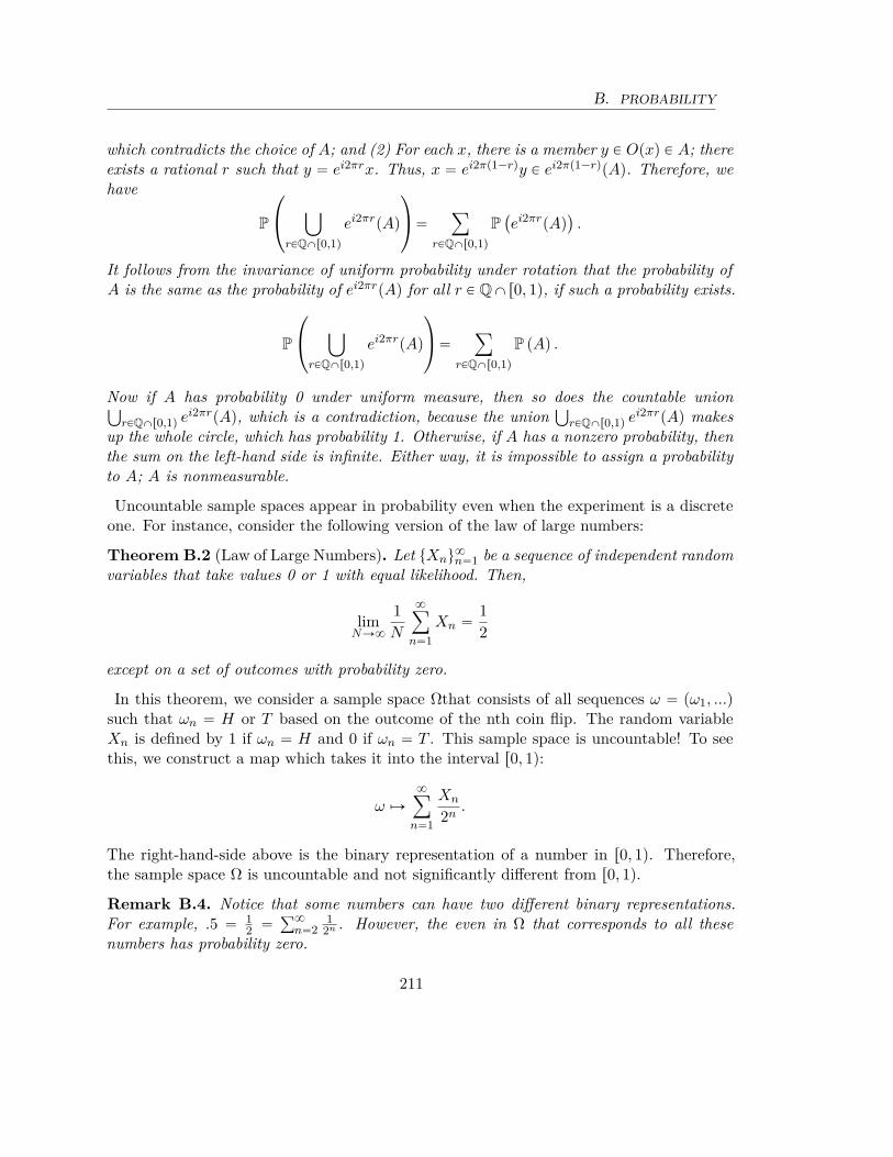
B. PROBABILITY
which contradicts the choice of A; and (2) For each x, there is a member y P Opxq P A; thereexists a rational r such that y “ ei2πrx. Thus, x “ ei2πp1´rqy P ei2πp1´rqpAq. Therefore, wehave
P
¨
˝
ď
rPQXr0,1q
ei2πrpAq
˛
‚“ÿ
rPQXr0,1q
P`
ei2πrpAq˘
.
It follows from the invariance of uniform probability under rotation that the probability ofA is the same as the probability of ei2πrpAq for all r P QX r0, 1q, if such a probability exists.
P
¨
˝
ď
rPQXr0,1q
ei2πrpAq
˛
‚“ÿ
rPQXr0,1q
P pAq .
Now if A has probability 0 under uniform measure, then so does the countable unionŤ
rPQXr0,1q ei2πrpAq, which is a contradiction, because the unionŤ
rPQXr0,1q ei2πrpAq makesup the whole circle, which has probability 1. Otherwise, if A has a nonzero probability, thenthe sum on the left-hand side is infinite. Either way, it is impossible to assign a probabilityto A; A is nonmeasurable.
Uncountable sample spaces appear in probability even when the experiment is a discreteone. For instance, consider the following version of the law of large numbers:
Theorem B.2 (Law of Large Numbers). Let tXnu8n“1 be a sequence of independent random
variables that take values 0 or 1 with equal likelihood. Then,
limNÑ8
1N
8ÿ
n“1Xn “
12
except on a set of outcomes with probability zero.
In this theorem, we consider a sample space Ωthat consists of all sequences ω “ pω1, ...qsuch that ωn “ H or T based on the outcome of the nth coin flip. The random variableXn is defined by 1 if ωn “ H and 0 if ωn “ T . This sample space is uncountable! To seethis, we construct a map which takes it into the interval r0, 1q:
ω ÞÑ
8ÿ
n“1
Xn
2n.
The right-hand-side above is the binary representation of a number in r0, 1q. Therefore,the sample space Ω is uncountable and not significantly different from r0, 1q.
Remark B.4. Notice that some numbers can have two different binary representations.For example, .5 “ 1
2 “ř8
n“21
2n . However, the even in Ω that corresponds to all thesenumbers has probability zero.
211
B. PROBABILITY
Events and their probability in a general setting
One of the important notions in the probability theory is dealing with the definition of anevent, a random variable, and the information related to them, which is presented in thefollowing definition.
Definition B.3 (σ-field). For a (possibly uncountable) sample space Ω, the set of eventsshould use the notion of σ-field from measure theory. A σ-field F is a collection of subsetsof Ω that satisfies
a) H and Ω P F .
b) If A P F , then AA P F .
c) For a sequence tAnu8n“0 Ď F ,
Ť8n“0 An P F .
A sample space Ω along with a σ-field is called a measurable space.
Usually, a σ-field can be specified by defining a set of elementary events and expandingthis set to a whole σ-field, which contains all events. For instance, in a discrete samplespace Ω “ tω1, ω2, ...u, one can define the elementary events to be En “ tωnu. Then, anyevent is a countable union of elementary events.In uncountable sample spaces, the methodology of working with elementary events is
inevitable. We consider a set of elementary events tEn : n ě 1u and construct thesmallest σ-field that contains all these elementary events, namely the σ-field generated byelementary sets tEn : n ě 1u denoted by σpEn : n ě 1q.
Example B.20. Consider Ω “ R and the elementary events given by the singleton setsEn :“ txnu for n “ 1, 2, .... Then, by property (b) the complement of singleton elementaryevents, EA
n “ Rztxnu is in the σ-field generated by Ens. Also, any finite or countablenumber of xns and the complement of it make events in this σ-field. For instance, theσ-field generated by t1u is
!
H,R, t1u,Rzt1u
)
.
The σ-field generated by t1u and t2u is!
H,R, t1u, t2u, t1, 2u,Rzt1u,Rzt2u,Rzt1, 2u
)
.
Example B.21. The σ-field generated by a single event, A has four distinct events: H,Ω, A, and AA. For example, the σ-field generated by the set of all rational numbers in Rconsist of H, R, the set of rational numbers, and the set of irrational numbers.
In the discrete example from the last paragraph, the σ-field is the same as the set of allsubsets of Ω. In Chapter 2, the sample space is Ω “ pRd`1qT . We consider each elementary
212
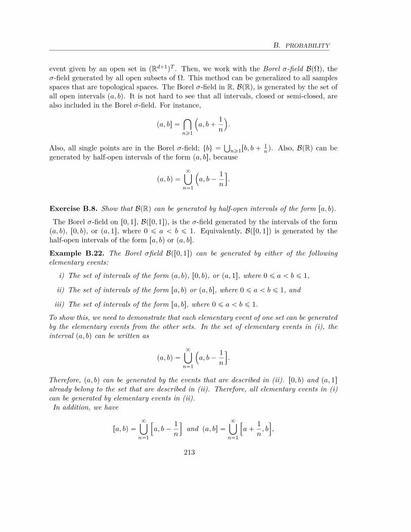
B. PROBABILITY
event given by an open set in pRd`1qT . Then, we work with the Borel σ-field BpΩq, theσ-field generated by all open subsets of Ω. This method can be generalized to all samplesspaces that are topological spaces. The Borel σ-field in R, BpRq, is generated by the set ofall open intervals pa, bq. It is not hard to see that all intervals, closed or semi-closed, arealso included in the Borel σ-field. For instance,
pa, bs “č
ně1
´
a, b `1n
¯
.
Also, all single points are in the Borel σ-field; tbu “Ť
ně1rb, b ` 1nq. Also, BpRq can be
generated by half-open intervals of the form pa, bs, because
pa, bq “
8ď
n“1
´
a, b ´1n
ı
.
Exercise B.8. Show that BpRq can be generated by half-open intervals of the form ra, bq.
The Borel σ-field on r0, 1s, Bpr0, 1sq, is the σ-field generated by the intervals of the formpa, bq, r0, bq, or pa, 1s, where 0 ď a ă b ď 1. Equivalently, Bpr0, 1sq is generated by thehalf-open intervals of the form ra, bq or pa, bs.
Example B.22. The Borel σfield Bpr0, 1sq can be generated by either of the followingelementary events:
i) The set of intervals of the form pa, bq, r0, bq, or pa, 1s, where 0 ď a ă b ď 1,
ii) The set of intervals of the form ra, bq or pa, bs, where 0 ď a ă b ď 1, and
iii) The set of intervals of the form ra, bs, where 0 ď a ă b ď 1.
To show this, we need to demonstrate that each elementary event of one set can be generatedby the elementary events from the other sets. In the set of elementary events in (i), theinterval pa, bq can be written as
pa, bq “
8ď
n“1
´
a, b ´1n
ı
.
Therefore, pa, bq can be generated by the events that are described in (ii). r0, bq and pa, 1s
already belong to the set that are described in (ii). Therefore, all elementary events in (i)can be generated by elementary events in (ii).In addition, we have
ra, bq “
8ď
n“1
”
a, b ´1n
ı
and pa, bs “
8ď
n“1
”
a `1n
, bı
,
213

B. PROBABILITY
which implies that all elementary events in (ii) can be generated by elementary events in(iii).
Finally, we have
ra, bs “
8č
n“1
´
a ´1n
, b `1n
¯
, pa, 1s “
8č
n“1
´
a ´1n
, 1ı
, and r0, bq “
8č
n“1
”
0, b `1n
¯
.
Therefore, all elementary events in (iii) can be generated by elementary events in (i).
The Borel σ-field on the half-line r0, 8q, Bpr0, 8qq, is the σ-field generated by the sets ofthe form pa, bq or r0, bq, where 0 ď a ă b.
Exercise B.9. Show that Bpr0, 8qq can be generated by either of the following elementaryevents:
i) The set of intervals of the form pa, bq or r0, bq, where 0 ď a ă b ď 1, and
ii) The set of intervals of the form ra, bq, where 0 ď a ă b ď 1.
Hint: Show that each elementary event of one set can be generated by the elementary eventsfrom the other set.
The following example is a useful use of elementary events in analyzing an event of interestand a method of finding the probability of such an event.
Example B.23. In Example B.13, let the event of ruin A be the collection of all outcomesfor which the gambler’s wealth eventually hits zero. For instance, if W0 “ 10, any outcomewith ten loses in a row since the start of the game is in this set. Also, any outcome with thenumber of losses at some time larger than the number of wins plus ten is in the ruin eventA. The ruin event is uncountable. We attempt to find the probability of this event later inExample B.25, namely the ruin probability. Before that, we need to write this event as aunion of disjoint simpler events for which the probability can easily be evaluated.
A “
8ď
¨
n“1An,
where An is the event that the ruin happens exactly at the nth round. Notice that An ismade of all outcomes such that (1) the nth round is a lost round, (2) in the first n ´ 1strounds there are x ´ 1 lost rounds more than the number of wins. Therefore, if m is thenumber of won rounds in the n´1st rounds, we must have 2m`x´1 “ n´1, or m “ n´x
2 .As a result, An is a nonempty event if and only if n ´ x is an even number. Therefore, onecan write
A “
8ď
¨
m“1Ax`2m.
214
B. PROBABILITY
Exercise B.10. Show that in Example B.23 the event of ruin is uncountable.
Many complicated sets can be found in the Borel σ-field. For more discussion of Borelsets, see [4, Chapter 7]. However, in most cases, it is enough to work with the elementaryevents that build the σ-field.Next, we define a probability measure in the most general form.
Definition B.4. A measure space is a pΩ, Fq such that Ω is a sample space and F is aσ-field on Ω. A measure on a measure space pΩ, Fq is a function from P : F Ñ R Y t8u
such that for any sequence tAnu8n“0 Ď F of disjoint events,
P
˜
8ď
n“0An
¸
“
8ÿ
n“0PpAnq.
A probability measure is a measure with the following properties.
a) For any A P F then PpAq ě 0.
b) PpΩq “ 1.
Notice that the above definition leads to many important properties of the probability:
a) PpAAq ` PpAq “ PpAA Y Aq “ PpΩq “ 1. Therefore, PpAAq “ 1 ´ PpAq.
b) PpHq “ 1 ´ PpΩq “ 0.
c) Continuity of probability. For any shrinking sequence of events A1 Ě A2 Ě ¨ ¨ ¨ ,we have
limnÑ8
PpAnq “
˜
8č
n“0An
¸
Exercise B.11. Show (c) in the above.
Triple pΩ, F ,Pq is called a probability space. To define any other measure P on a mea-surable space pΩ, Fq, it is sufficient to define it on the elementary sets that generate theσ-field F . For example, to define a uniform probability measure on r0, 1s on the Borelσ-field Bpr0, 1sq, one only needs to define
Pppa, bqq “ b ´ a, for pa, bq P r0, 1s.
Since probability of singleton is zero, we have
Ppr0, bqq “ Ppt0uq ` Ppp0, bqq “ 0 ` b.
Similarly, Pppa, 1sq “ 1 ´ a.Here is a more complicated example. The random variable in this example is not discrete
or continuous.
215
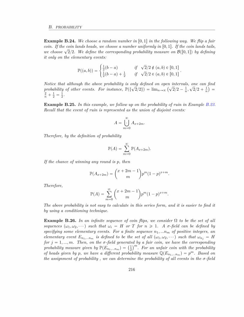
B. PROBABILITY
Example B.24. We choose a random number in r0, 1s in the following way. We flip a faircoin. If the coin lands heads, we choose a number uniformly in r0, 1s. If the coin lands tails,we choose
?22. We define the corresponding probability measure on Bpr0, 1sq by defining
it only on the elementary events:
Pppa, bqq “
#
12pb ´ aq if
?22 R pa, bq P r0, 1s
12pb ´ aq ` 1
2 if?
22 P pa, bq P r0, 1s.
Notice that although the above probability is only defined on open intervals, one can findprobability of other events. For instance, Ppt
?22uq “ limnÑ8
`?22 ´ 1
n ,?
22 ` 1n
˘
“2n ` 1
2 “ 12 .
Example B.25. In this example, we follow up on the probability of ruin in Example B.23.Recall that the event of ruin is represented as the union of disjoint events:
A “
8ď
¨
m“0Ax`2m.
Therefore, by the definition of probability
PpAq “
8ÿ
m“0PpAx`2mq.
If the chance of winning any round is p, then
PpAx`2mq “
ˆ
x ` 2m ´ 1m
˙
pmp1 ´ pqx`m.
Therefore,
PpAq “
8ÿ
m“0
ˆ
x ` 2m ´ 1m
˙
pmp1 ´ pqx`m.
The above probability is not easy to calculate in this series form, and it is easier to find itby using a conditioning technique.
Example B.26. In an infinite sequence of coin flips, we consider Ω to be the set of allsequences pω1, ω2, ¨ ¨ ¨ q such that ωi “ H or T for n ě 1. A σ-field can be defined byspecifying some elementary events. For a finite sequence n1, ...nm of positive integers, anelementary event En1,...nm is defined to be the set of all pω1, ω2, ¨ ¨ ¨ q such that ωnj “ Hfor j “ 1, ..., m. Then, on the σ-field generated by a fair coin, we have the correspondingprobability measure given by PpEn1,...nmq “
`12˘m. For an unfair coin with the probability
of heads given by p, we have a different probability measure QpEn1,...nmq “ pm. Based onthe assignment of probability , we can determine the probability of all events in the σ-field
216
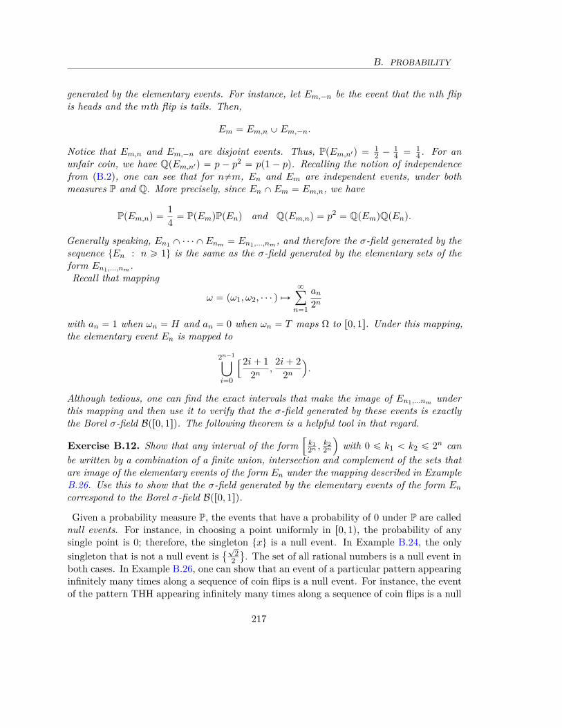
B. PROBABILITY
generated by the elementary events. For instance, let Em,´n be the event that the nth flipis heads and the mth flip is tails. Then,
Em “ Em,n Y Em,´n.
Notice that Em,n and Em,´n are disjoint events. Thus, PpEm,n1q “ 12 ´ 1
4 “ 14 . For an
unfair coin, we have QpEm,n1q “ p ´ p2 “ pp1 ´ pq. Recalling the notion of independencefrom (B.2), one can see that for n‰m, En and Em are independent events, under bothmeasures P and Q. More precisely, since En X Em “ Em,n, we have
PpEm,nq “14
“ PpEmqPpEnq and QpEm,nq “ p2 “ QpEmqQpEnq.
Generally speaking, En1 X ¨ ¨ ¨ X Enm “ En1,...,nm, and therefore the σ-field generated by thesequence tEn : n ě 1u is the same as the σ-field generated by the elementary sets of theform En1,...,nm.Recall that mapping
ω “ pω1, ω2, ¨ ¨ ¨ q ÞÑ
8ÿ
n“1
an
2n
with an “ 1 when ωn “ H and an “ 0 when ωn “ T maps Ω to r0, 1s. Under this mapping,the elementary event En is mapped to
2n´1ď
i“0
”2i ` 12n
,2i ` 2
2n
¯
.
Although tedious, one can find the exact intervals that make the image of En1,...nm underthis mapping and then use it to verify that the σ-field generated by these events is exactlythe Borel σ-field Bpr0, 1sq. The following theorem is a helpful tool in that regard.
Exercise B.12. Show that any interval of the form”
k12n , k2
2n
¯
with 0 ď k1 ă k2 ď 2n canbe written by a combination of a finite union, intersection and complement of the sets thatare image of the elementary events of the form En under the mapping described in ExampleB.26. Use this to show that the σ-field generated by the elementary events of the form En
correspond to the Borel σ-field Bpr0, 1sq.
Given a probability measure P, the events that have a probability of 0 under P are callednull events. For instance, in choosing a point uniformly in r0, 1q, the probability of anysingle point is 0; therefore, the singleton txu is a null event. In Example B.24, the onlysingleton that is not a null event is
?2
2(
. The set of all rational numbers is a null event inboth cases. In Example B.26, one can show that an event of a particular pattern appearinginfinitely many times along a sequence of coin flips is a null event. For instance, the eventof the pattern THH appearing infinitely many times along a sequence of coin flips is a null
217
B. PROBABILITY
event.
Exercise B.13. Show that the event of the pattern THH (or any other particular pattern)appearing infinitely many times along a sequence of coin flips is a null event.
Random variables and integration
Before Andrey Kolmogorov used measures for probability, measures were used to extend thenotion of integration. Integration with respect to measures is also important in probabilitytheory to define the expected value of random variables. In this section, we explain thedefinition of a random variable and define the expected value of a random variable by theintegral of that random variable with respect to a probability measure in the most generalform, which included uncountable sample spaces.
Definition B.5. A random variable on a measure space pΩ, Fq is a function X : Ω Ñ Rd
such that for any Borel set A P BpRdq, the inverse image of A, X´1pAq, belongs to the setof events F .
Since B is generated by open sets, the condition “@A P BpRdq, X´1pAq P F” in DefinitionB.5 needs to hold only for all open sets instead of all Borel sets; A P BpRdq for all opensets A Ď Rd.If Ω “ Rd and F “ BpRdq, a random variable is called a Borel measurable function.In practice, important random quantities are described by random variables. See the
example below.
Example B.27. In an infinite sequence of coin flips, Example B.26, we define the randomvariable X as follows. For ω “ pω1, ω2, ¨ ¨ ¨ q P Ω
Xpωq “
8ÿ
n“1
an
3n
such that an “ 0 if ωn “ H, and an “ 2 if ωn “ T. Here,ř8
n“1an3n “ 0.a1a2 ¨ ¨ ¨ is the
ternary representation of a number in r0, 1s. X maps Ω to r0, 1s. To check if X is a randomvariable, we need to check that the inverse of an open interval is in the σ-field generated bythe elementary sets An1,...nm described in Example B.26. We leave this task to the followingexercise.
Remark B.5. The image of X in Example B.27 is called a Cantor set.
Exercise B.14. Show that the mapping X defined in Example B.27 is a random variable.Hint: Assume a ternary representation for the endpoints of the the interval pa, bq.
218

B. PROBABILITY
If a random variable X is defined on a probability space pΩ, F ,Pq, the expected value ofX is defined as an integral of X with respect to measure P, denoted by
ErXs :“ż
XdP.
The definition of the integral is a little cumbersome. Thus, we only outline the steps.
Step 1) For an indicator random variable X “ 1A where A is an event in F , we have
ErXs :“ż
AdP “ PpAq.
Step 2) For step random variable X, a finite linear combination of indicator randomvariables X “
řNj“1 aj1Aj , we have
ErXs :“Nÿ
j“1ajPpAjq.
Step 3) If the random variable X is nonnegative,X ě 0, then X can be approximatedfrom below by an increasing sequence of step random variables; Xn Ò X. Then,
ErXs :“ supn
ErXns.
Notice that one can show that the value ErXs is independent of the choice ofthe increasing sequence of step random variables and thus is well defined.
Step 4) For a general random variable X, we decompose X into positive and negativeparts; X “ X` ´ X´ with X` “ max 0, X and X´ “ max 0, ´X. Then,
ErXs :“ ErX`s ´ ErX´s.
In Step (4) in the above, the expected value ErXs is 8 when ErX`s “ 8 and ErX´s ă 8,and it is ´8 when ErX`s ă 8 and ErX´s “ 8. However, ErXs cannot be defined whenwe have both ErX`s “ 8 and ErX´s “ 8. This motivates the following definition.
Definition B.6. A random variable is called integrable if Er|X|s “ ErX`s ` ErX´s ă 8.
The following example shows why we need to separate the positive part and the negativepart of a random variable in Step 4 above.
Example B.28. Consider the uniform probability measure on probability space given byΩ “ r´1, 1s2, the two dimensional square, and a random variable X given by Xpx, yq “
219

B. PROBABILITY
xypx2`y2q2
11. The positive part of X is r0, 1s2 Y r´1, 0s2. It is easy (by switching to polarcoordinates) to see that
ż
r0,1s2
X`dP “
ż 1
0
ż 1
0
xy
px2 ` y2q2 dxdy `
ż 0
´1
ż 0
´1
xy
px2 ` y2q2 dxdy “ 8,
and therefore, X is not integrable. We conclude that ErXs does not exist. However, theiterated integral below exists and is equal to zero, i.e.
ż 1
´1
ż 1
´1Xpx, yqdxdy “ 0.
Therefore, for random variable X, the iterated integral is not a well defined notion ofexpectation.
There are three main convergence theorems for integrals with respect to a measure, whichare very useful in the probability theory. We conclude this section by presenting them.
Theorem B.3 (Monotone convergence theorem). Let tXnuně1 be a sequence of nonneg-ative and increasing random variables. Then, X :“ limnÑ8 Xn is a random variable andErXs “ limnÑ8 ErXns.
Example B.29. In Example B.27, we assume the coin is a fair coin. We shall find theexpected value of the introduced random variable by introducing the sequence of randomvariables tXnu8
n“1 defined by
Xnpωq :“nÿ
j“1
aj
3j,
such that aj “ 0 if ωj “ H, and aj “ 2 if ωj “ T. Notice that by the monotone convergencetheorem, limnÑ8 ErXns “ ErXs. Observe that Xn “ Xn´1 ` ξn, where ξn takes two values0 and 2
3n with equal probabilities 12 . Therefore, ErXns “ ErXn´1s`Erξns. Since Erξns “ 1
3n ,we have ErXns “ ErXn´1s ` 1
3n . By solving ErXns “ ErXn´1s ` 13n recursively, we obtain
ErXns “řn
j“113j . As n Ñ 8, if follows from the monotone convergence theorem that
ErXs “ř8
j“113j “ 1
2 .
Exercise B.15. Repeat the calculation in Example B.29 for an unfair coin with a proba-bility p of heads.
Theorem B.4 (Fatou’s lemma). Let tXnuně1 be a nonnegative sequence of random vari-ables. Then, X “ lim infnÑ8 Xn is a random variable, and ErXs ď lim infnÑ8 ErXns.
11X is undefined at the single point p0, 0q. But, the probability of a single point is 0. Therefore, we candefine Xp0, 0q by any value of choice; for example, Xp0, 0q “ 0.
220

B. PROBABILITY
Example B.30. On the sample space Ω “ r0, 1q equipped with uniform probability measure,define the sequence of random variables tYnu8
n“1 by
Ynpωq “
#
1 when for j “ 1, ..., n, aj “ 0 or 20 otherwise
,
where ω “ř8
j“1aj
3n is the ternary expansion of ω P Ω. Define
Y pωq :“ limnÑ8
Ynpωq.
It is straightforward to see that
Y pωq “
#
1 when aj “ 0 or 2 for all j ě 10 otherwise
.
In other words, Y is the indicator random variable of the event that contains all numbersin r0, 1q whose ternary representation has only digits 0 or 2. This event is the same as theCantor set in Remark B.5 and is denoted by C. Therefore, Y “ 1C and ErY s “ PpCq. Tofind the PpCq, we use Fatou’s lemma, Theorem B.4, and write
ErY s “ PpCq ď lim infnÑ8
ErYns.
Next, we will show that lim infnÑ8 ErYns “ 0. To see this, first observe that Yn is alsoan indicator random variable. For example for n “ 1, Y1 “ 1r0,13qYr23,1q and Y2 “
1r0,19qYr29,13qYr23,79qYr89,1q, and so on. Generally speaking,
Yn “ 1An ,
where An is the union of 2n intervals each of size 13n . Therefore, under uniform probability,
ErYns “ PpAnq “2n
3nÑ 0, as n Ñ 8.
This means that the Cantor set has a probability of 0 under uniform probability.
Theorem B.5 (Lebesgue convergence theorem). Let tXnuně1 be a convergent sequence ofrandom variables and ξ be an integrable random variable such that |Xn| ď |ξ| for all n ě 1.Then, X :“ limnÑ8 Xn is a random variable, and ErXs “ limnÑ8 ErXns.
Remark B.6. In Example B.30, we could use Lebesgue convergence theorem, TheremB.5, to show that ErY s “ 0. This is because all random variables Yn are indicators, andtherefore, their absolute values are bounded by the constant random variable ξ “ 1.
221
B. PROBABILITY
Equality of random variables
Recall the simple version of the law of large numbers in Theorem B.2. Here, we put theemphasis on the exception set, where the limit inside the theorem does not converge to 1
2 .One possible outcome inside this set is given by Xn “ 0 for n ” 0 pmod 3q, and Xn “ 1for n ” 1 or 2pmod 3q. Then, the limit on the left-hand side converges to 2
3 , not 12 . The
law of large numbers in Theorem B.2 asserts that the collection of all outcomes such thatlimNÑ8
1N
řNn“1 Xn exists and is equal to 1
2 is an event with a probability of 1. In otherwords, the random variable limNÑ8
1N
řNn“1 Xn is defined to be the constant 1
2 except onan event with probability 0.
Definition B.7. Two random variables X and Y are considered equal if the event
tω P Ω : Xpωq‰Y pωqu
has a probability of zero. Then, we write X “ Y P almost surely; X “ Y P-a.s. for short;or just a.s. whenever the probability measure is assumed.
For instance, Theorem B.2 indicates that the random variable on the left-hand side,limNÑ8
1N
ř8n“1 Xn, is equal to the random variable on the right-hand side, 1
2 , a.s. Inaddition, it also implies that the limit limNÑ8
1N
ř8n“1 Xn exists a.s., which is not an
obvious fact.As a result of the following Lemma, Theorem B.2 shows that the random variable Xpωq “
limNÑ8
řNn“1 Xn ´ 1
2 is zero a.s.: a very fancy representation for zero!
Lemma B.1. For a nonnegative random variable X, ErXs “ 0 if and only if X “ 0 a.s.
As a consequence, we can define the convergence of a sequence of random variables.
Definition B.8. A sequence tXnu8n“1 of random variables is called convergent a.s. if the
eventtω P Ω : lim
nÑ8Xnpωq does not existu
has a probability of 0. Then, the limit random variable X :“ limnÑ8 Xn exists a.s. and iscalled the limit of tXnu8
n“1.
Law of a random variable
In the remainder of this section, we show how to define expectation for general random vari-ables by means of the distribution function, without appealing to the notion of integrationwith respect to a measure.
Definition B.9. For a random variable X with real values, the cumulative distributionfunction (or cdf or simply “distribution function”) FXpxq is defined by
FXpxq :“ PpX ď xq.
222

B. PROBABILITY
The definition of a distribution function is related to the probability measure P by PpX P
pa, bsq “ FXpbq ´ FXpaq. In fact, the distribution function induces a probability measureon R, denoted by PX , which is defined on open intervals by
PXppa, bsq “ FXpbq ´ FXpaq.
recall that to define a probability measure on BpRq, we only need to define it on the openintervals, or equivalently on the half-open intervals of the form pa, bs.
Example B.31. Let X “ 1A. Then, FXpxq “ 0 if x ă 1 and FXpxq “ 1 if x ě 1; seeFigure B.4.
1
1
x
FX(x)
Figure B.4: The distribution function for an indicator.
Example B.32. In Example B.24, define a random variable that is equal to the value ofthe picked random number. Then, the law of X is shown in Figure B.5.
For a discrete random, FX is a step function. For nondiscrete random variables FXpxq isnot a step function. The distribution function of random variable X in Example B.27 isillustrated in Figure B.612.In general, the distribution function of a random variable X satisfies the following prop-
erties.
a) FXp´8q “ 0 and FXp8q “ 1.
b) FX is an increasing right-continuous function with a left-limit at all points.12To be precise, the distribution function of random variable X in Example B.27 is approximated by the
distribution function of random variable Xn with a large n.
223

B. PROBABILITY
√22
1
√24
12 +
√24
x
FX(x)
Figure B.5: The distribution function for the random number chosen in Example B.24.
0 0.2 0.4 0.6 0.8 1
0
0.2
0.4
0.6
0.8
1
Figure B.6: Devil’s Staircase: the distribution function of the random variable X inExample B.27.
Exercise B.16. Show that PpX P ra, bsq “ FXpbq ´ FXpa´q, where FXpa´q is the leftlimit of FX at a.
It is also well known that if a function F satisfies the properties (a) and (b) of a distributionfunction, then there is always a random variable X in a proper sample space such thatFX “ F .The probability PX is called the law of X. Notice that knowing FX and knowing the law
224
B. PROBABILITY
of X are equivalent, but they are not equivalent to knowing P. In fact, we shall see that inmany important calculations about random variables, we do not exactly need to know P;in most applications, the law of a random variable is all we need. Therefore, we will nowintroduce expected value in terms of the law of the random variable.Notice that FX is an increasing function, and therefore one can define the Riemann-
Stieltjes integral with respect to FX as an alternative to the more complicated notion ofintegration with respect to measure P. In this case, the integral with respect to measurePX is also simplified to a Riemann-Stieltjes13 integral.
Proposition B.3. For an integrable random variable X the expectation of X satisfies
ErXs “
ż 8
´8
xdFXpxq.
In particular, for any function g,
ErgpXqs “
ż 8
´8
gpxqFXpdxq,
given Er|gpXq|s ă 8.
Similarly, for a random vector X “ pX1, ..., Xdq, the distribution function is defined by
FXpx1, ..., xdq :“ PpX1 ď x1, ..., Xd ď xdq.
The law of X is a probability measure PX on Rd such that
PXpp´8, x1s ˆ ¨ ¨ ¨ ˆ p´8, xdsq “ FXpx1, ..., xdq.
Then, the expectation of gpX1, ..., Xdq is given by
ErgpX1, ..., Xdqs “
ż 8
´8
gpx1, ..., xdqFXpdx1, ..., dxdq,
given Er|gpX1, ..., Xdq|s ă 8.
Exercise B.17. If tXiu8i“1 is a sequence of independent Bernoulli random variables with
equally likely values 0 and 1, show that U “ř8
i“1Xi2i is uniformly distributed on r0, 1s.
Conditional expectation
Conditional expectation cannot simply be defined in terms of the distribution function;more advanced methods are needed. Unlike discrete probability setting, (B.5) in Section B,
13Read“Steel-chess”.
225

B. PROBABILITY
we need to define ErX | Y s in general form by using a powerful tool in analysis, namely theRadon-Nikodym theorem. To give you a glimpse of the definition, we recall from RemarkB.3 in the discrete setting that ErX | Y “ ys is a function of the variable y, denotedby hpyq. Then we use this function to define ErX | Y s by hpY q. Similarly, we try tofind ErX | Y s among the random variables of the form hpY q for some (Borel measurable)function h : R Ñ R.
Definition B.10 (Conditional expectation). Let X be an integrable random variable.ErX | Y s is the unique random variable of the form hpY q, where h : R Ñ R is a Borelmeasurable function that satisfies
ErhpY qgpY qs “ ErXgpY qs, (B.6)
for all real bounded functions g with domain containing the set of values of Y such thatXgpY q is integrable.
The Radon-Nikodym theorem from measure theory guarantees the existence and unique-ness of an integrable random variable ErX | Y s in the a.s. sense. Given Definition B.10 forconditional expectation, all the results of Corollary B.2, Proposition B.1, and PropositionB.3 hold for general random variables.
Corollary B.4. Let X and Y be random variables and f be a real function, such thatfpY qX is integrable. Then,
ErfpY qX | Y s “ fpY qErX | Y s.
Proposition B.4. X and Y are independent if and only if for any real function fpx, yq
of X and Y we have
ErfpX, Y q | Y “ ys “ ErfpX, yqs for all y in the set of values of Y,
provided that both fpX, Y q and fpX, yq are integrable for all y in the set of values of Y .
Corollary B.5. Let X and Y be independent and f be a real function such that fpXq isintegrable. Then,
ErfpXq | Y s “ ErfpXqs.
Proposition B.5 (Tower property of conditional expectation). Let X, Y and Z be randomvariables. Then,
ErErX | Y, Zs | Y s “ ErX | Y s.
In particular,ErErX | Y ss “ ErXs.
Remark B.7. The two following comments often helps in finding conditional expectationin the general form.
226
B. PROBABILITY
1) One can verify (B.10) over a smaller set of functions to guarantee ErX | Y s “ hpY q.For instance, if for any bounded function g we have ErhpY qgpY qs “ ErXgpY qs, thenErX | Y s “ hpY q holds true. Equivalently, if for any Borel set (or open set) A wehave ErhpY q1Y PAs “ ErX1Y PAs, then ErX | Y s “ hpY q.
2) If for a constant a, Aa “ tY “ au is an event with positive probability, then ErX |
Y “ as “ hpaq and is also constant. Then, on can find constant hpaq by usingErhpY q1Y PAas “ ErX1Y PAas in the following.
ErhpY q1tY PAaus “ hpaqPpY “ aq “ ErX1tY PAaus ùñ hpaq “ErX1tY PAaus
PpY “ aq.
This means the conditional expectation ErX | Y s on the event Y=a is constant andis equal to the average of X over the event tY “ au.
Exercise B.18. Use Remark B.7 to show Corollary B.4, Proposition B.4 and PropositionB.5.
Exercise B.19. Show that X and Y are independent if and only if for any two realfunctions h1pxq and h2pyq we have
Erh1pXqh2pY qs “ Erh1pXqsErh2pY qs. (B.7)
Let X be a random variable. The σ-field generated by X, is the smallest σ-field whichcontains all events tX P Au for all Borel sets A, and is denoted by σpXq. In other word,the σpXq which contains all events related to X. σpXq can equivalently be expressed asthe smallest σ-field which contains all events tX P Au for all open sets A. We say arandom variable Z is σpXq-measurable, measurable with respect to σpXq, if for any Borelset A, the event tZ P Au is in σpXq. It is known that if Z is σpXq-measurable, then thereexists a Borel function h : R Ñ R such that Z “ hpXq. In particular, since ErX | Y s isY -measurable, ErX | Y s “ hpY q.More generally, for a σ-field G Ď F , one can define ErX | Gs; the conditional expectation
of X given the events in G. The definition is similar to Definition B.10, for which theexistence and uniqueness is guaranteed by Radon-Nykodim theorem.
Definition B.11 (Conditional expectation with respect to σ-field). Let X be an integrablerandom variable and G be a sub σ-field of F . ErX | Gs is the unique random variable Zwhich satisfies
ErZY s “ ErXY s, (B.8)
for all G-measurable random variables Y such that XY is integrable.
Remark B.7 holds also for (B.11); one can only verify ErZ1Gs “ ErX1Gs, for all G P Gthen Z “ ErX | Gs. If G is generated by a set of elementary events E , then one only needs
227

B. PROBABILITY
to verify that ErZ1Es “ ErX1Es for all E P E . In addition, if A is an event in G such thatPpAq ą 0 and for any events B P G such that B Ď A, we have PpBq “ PpAq or PpBq “ 0,then on A we have
ErX | Gs “ErX1tY PAus
PpAq.
Exercise B.20. Consider the probability space pp0, 1q, Bpp0, 1qqq,Pq where P is uniformprobability measure, and let G be the σ-field generated by the intervals p i
4 , i`14 q, for i “
0, 1, 2, 3. Define the random variable X : ω P p0, 1q ÞÑ R to be Xpωq “ 1p13,23q ´ 1p0,13q ´
1p23,1q. We would like to find ErX|Gs. The key observation here is that the σ-field G canbe generated by a random variable which takes a constant values in interval p i
4 , i`14 q, for
i “ 0, 1, 2, 3. For instance one can choose (among all other valid choices)
Y “
3ÿ
i“0i1
p i4 , i`1
4 q
and ErX|Gs “ ErX|Y s. Therefore, since Y is constant in each interval p i4 , i`1
4 q, so isErX|Gs, and we can write
ErX|Gs “
3ÿ
i“0ai1p i
4 , i`14 q
.
In Definition B.11, one can take Y “ 1p i
4 , i`14 q
to obtain
aiEr1p i
4 , i`14 q
s “ ErX1p i
4 , i`14 q
s “
ż i`14
i4
Xpωqdω “
$
’
’
’
’
&
’
’
’
’
%
´14 i “ 0
112 i “ 1112 i “ 2´1
4 i “ 3
Therefore,
ai “
$
’
’
’
’
&
’
’
’
’
%
´1 i “ 013 i “ 113 i “ 2´1 i “ 3
andErX|Gs “ ´1p0, 1
4 q `13
1p 14 , 1
2 q `13
1p 12 , 3
4 q ´ 1p 34 ,1q.
and
The conditional expectation ErX | Gs can be understood by using the concept of regression.Consider the vector space of square integrable random variables; i.e., V “ tξ : Erξ2s ă 8u
and a linear subspace W of V including all G-measurable random variables. Then, for a
228
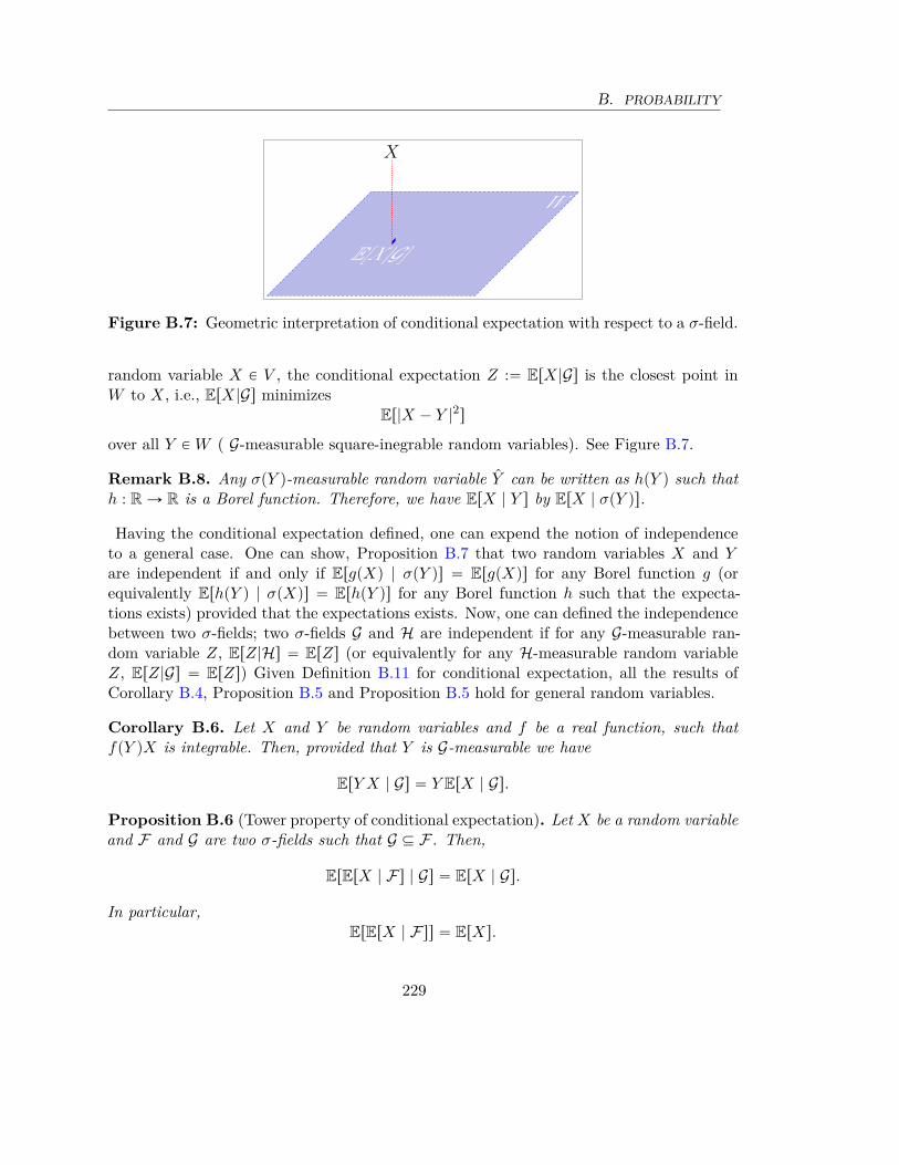
B. PROBABILITY
X
E[X|G]
W
Figure B.7: Geometric interpretation of conditional expectation with respect to a σ-field.
random variable X P V , the conditional expectation Z :“ ErX|Gs is the closest point inW to X, i.e., ErX|Gs minimizes
Er|X ´ Y |2s
over all Y P W ( G-measurable square-inegrable random variables). See Figure B.7.
Remark B.8. Any σpY q-measurable random variable Y can be written as hpY q such thath : R Ñ R is a Borel function. Therefore, we have ErX | Y s by ErX | σpY qs.
Having the conditional expectation defined, one can expend the notion of independenceto a general case. One can show, Proposition B.7 that two random variables X and Yare independent if and only if ErgpXq | σpY qs “ ErgpXqs for any Borel function g (orequivalently ErhpY q | σpXqs “ ErhpY qs for any Borel function h such that the expecta-tions exists) provided that the expectations exists. Now, one can defined the independencebetween two σ-fields; two σ-fields G and H are independent if for any G-measurable ran-dom variable Z, ErZ|Hs “ ErZs (or equivalently for any H-measurable random variableZ, ErZ|Gs “ ErZs) Given Definition B.11 for conditional expectation, all the results ofCorollary B.4, Proposition B.5 and Proposition B.5 hold for general random variables.
Corollary B.6. Let X and Y be random variables and f be a real function, such thatfpY qX is integrable. Then, provided that Y is G-measurable we have
ErY X | Gs “ Y ErX | Gs.
Proposition B.6 (Tower property of conditional expectation). Let X be a random variableand F and G are two σ-fields such that G Ď F . Then,
ErErX | Fs | Gs “ ErX | Gs.
In particular,ErErX | Fss “ ErXs.
229
B. PROBABILITY
Proposition B.7. X is independent of all G-measurable random variables if and only iffor any bounded f real function such that fpXq is integrable, we have
ErfpXq | Gs “ ErfpXqs.
In particular, X is independent of Y if and only if ErfpXq | σpY qs “ ErfpXqs.
Corollary B.7. Consider a probability space pΩ, F ,Pq which hosts a random variable Xand let G be a σ-field such that G Ď F . Then for any convex function f , we have
fpErX | Gsq ď ErfpXq | Gs,
provided that both of the expectations exist.
The proof of this corollary is exactly the same line of argument as in Corollary B.1.
Continuous random variables
In this section, we review basic concepts of continuous random variables without referringto measurability issues. Therefore, a gap on the rigorousness of the concepts remainsthroughout this section.
Definition B.12. A random variable X is called continuous if there exits a nonnegativemeasurable function fX : Rd Ñ R such that
FXpxq :“ż x1
´8
¨ ¨ ¨
ż xd
´8
fXpyqdy.
In this case, the function fX is called probability density function (pdf) of the continuousrandom variable X.
Working with continuous random variables is often easier since one can easily approxi-mate the integrals to estimate relevant quantities. For example, when X in a univariatecontinuous random variable with pdf fX , expectation of X is given by
ErXs “
ż 8
´8
xfXpxqdx.
More generally, for a function h : R Ñ R, we have
ErhpXqs “
ż 8
´8
hpxqfXpxqdx.
If I Ď R, thenPpX P Iq “
ż
IfXpxqdx.
230
B. PROBABILITY
Example B.33 (Normal distribution). A continuous random variable X with density
fXpxq “1
?2π
e´ x22 for all x P R
is called standard normal random variable. By using integration techniques, one can seethat ErXs “ 0 and varpXq :“ ErX2s “ 1.If Y “ σX ` µ for σ ą 0 and µ P R, then Y is also a continuous random variable with
density
fY pxq “1
?2πσ
e´px´µq2
2σ2 for all x P R.
Then, Y is called a normal random variable with mean µ and variance σ2 and is denotedby Y „ N pµ, σ2q.
Exercise B.21. Show that when X „ N p0, 1q, we have ErXs “ 0 and varpXq :“ ErX2s “
1.
When X “ pX1, ..., Xdq is a jointly continuous random vector, we refer to pdf as thejoint probability distribution of X1, ..., Xd to emphasize on the multi-dimensionality. Forsimplicity, let’s focus on two random variables. Let the joint pdf of pX, Y q be fX,Y px, yq.Then, it is easy to see that
a) pdf of X, fX satisfies
fXpxq “
ż 8
´8
fX,Y px, yqdy.
Similar formula holds for the pdf of Y .
b) for a function h : R2 Ñ R, we have
ErhpXqs “
ż 8
´8
ż 8
´8
hpx, yqfX,Y px, yqdxdy
c) if K Ď R2, thenPppX, Y q P Kq “
ij
K
fX,Y px, yqdA.
Example B.34 (Bivariate normal distribution). Let C be a symmetric positive-definitematrix and µ “ pµ1, ..., µdq P Rd. A jointly continuous random vector X “ pX1, ..., Xdq
with densityfXpxq “
1p2πdetpCqqd2 e´
px´µqC´1px´µqT2 for all x P Rd
231
B. PROBABILITY
is called multi-variate normal random vector. For each j “ 1, ..., d, ErXjs “ µj. The matrixC is called the covariance matrix of X, because its entities correspond to the covariance ofcomponents of X, i.e.
Ci,j “ ErpXi ´ µiqpXj ´ µjqs.
In particular, for d “ 2, for a positive-definite matrix14
C “
„
σ21 σ12
σ12 σ22
ȷ
and µ “ 0, we have
fX,Y px, yq “1
2πa
σ21σ2
2 ´ σ212
e´
σ22x2´2σ12xy`σ2
1y2
2pσ21σ2
2´σ212q for all x P R.
Here by evaluating double integrals, we can see that σ21 and σ2
2 are variance of X and Yrespectively, and σ12 is the covariance of X and Y .
Exercise B.22. In Example B.34, show that covpX, Y q :“ ErpXi ´ µiqpXj ´ µjqs “ Ci,j.
Exercise B.23. In Example B.34, show that σ21 and σ2
2 are variance of X and Y respec-tively, and σ12 is the covariance of X and Y .
Defining and calculating conditional probability and conditional expectation is also donethrough integral definition for continuous random variables. Let pX, Y q be a jointly con-tinuous random variable with density fX,Y px, yq. Then, the conditional density of X givenY “ y is defined by
fX|Y px | yq :“ fX,Y px, yq
fY pyq,
provided that y be in the set of values of Y , i.e., ty : fpyq ‰ 0u. Using the above definition,the conditional probability of X P I given Y “ y is given by
PpX P I | Y “ yq :“ş
I fX,Y px, yqdx
fpyq(B.9)
Similarly, if h : R Ñ R be a function, then the conditional expectation of hpXq given Y “ yis given by
ErhpXq | Y “ ys :“ş8
´8hpxqfX,Y px, yqdx
fpyq. (B.10)
14In order for C to be positive-definite, is necessary and sufficient to have σ1, σ2 ‰ 0 and σ21σ2
2 ´ σ212 ą 0.
232

B. PROBABILITY
In particular, the conditional expectation of X given Y “ y is given by
ErX | Y “ ys :“ş8
´8xfX,Y px, yqdx
fY pyq. (B.11)
Notice that conditional expectation and conditional probability in (B.9), (B.10), and(B.11)are functions of the variable y. The domain of all these is the set of values of Y , i.e.,ty : fY pyq ‰ 0u. This, in particular, can be useful in defining conditional distribution andconditional probability given Y . Let’s first make the definition for conditional probabilityof X P I given Y . Define the function Y of y which maps y onto PpX P I | Y “ yq :“ş
I fX,Y px,yqdx
fY pyq. Then, one can define
PpX P I | Y q :“ YpY q “
ş
I fX,Y px, Y qdx
fY pY q.
Notice that unlike PpX P I | Y “ yq which is a real function, PpX P I | Y q is a randomvariable which is completely dependent on random variable Y . Similarly we have
ErhpXq | Y s :“ş8
´8hpxqfX,Y px, Y qdx
fY pY qand ErX | Y s :“
ş8
´8xfX,Y px, Y qdx
fY pY q.
For continuous random variables independence can be defined in terms of the joint pdffpx, yq; let X and Y be jointly continuously. Then, X and Y are called independent if fis a separable function, i.e.
fX,Y px, yq “ gpxqhpyq.
Notice that the choice of h and g is not unique and varies by multiplying or dividingconstants. In this case, one can write the separation in a standard form
fX,Y px, yq “ fXpxqfY pyq, (B.12)
where fXpxq and fY pyq are respectively the pdf of x and pdf of Y .
Example B.35. From Example B.34 and (B.12), one can see bivariate normal randomvariables are independent if and only if they are uncorrelated, i.e., they have zero correlationor simply σ12 “ 0.
Exercise B.24. Show that (B.7) and (B.12) are equivalent.
B.3 Martingales
The conditional expectation defined in the previous section is required to define martingale.Consider a probability space pΩ, F ,Pq, i.e., sample space Ω, a σ-field and a probability
233
B. PROBABILITY
measure P, and let X :“ tXtuTt“0 (possibly T “ 8) be a discrete-time stochastic process;
for any t, Xt is a random variable.
Definition B.13. A discrete-time stochastic process tMtuTt“0 on a probability space pΩ, F ,Pq
is called a martingale with respect to X if
a) Mt is integrable for all t “ 0, ..., T , i.e., Er|Mt|s ă 8.
b) the conditional expectation Mt given Xs, Xs´1, ..., X0 is equal to Ms, i.e., ErMt|Xs, Xs´1, ..., X0s “
Ms, for s ă t.
Condition (a) in the definition of martingale is technical and guarantees the existence ofthe conditional expectation in condition (b). Condition (b) can also be given equivalentlyby
b’) ErMt|Xt´1, ..., X0s “ Mt´1, for t ě 1.
Notice that as a result of tower property of conditional expectations, if (b’) holds we canwrite
ErErMt|Xt´1, ..., X0s|Xs, ..., X0s “ ErMt´1|Xs, ..., X0s.
By applying the tower property in Proposition B.5 inductively, we obtain
ErErMt| Xt´1, ..., Xs`1looooooomooooooon
Z
, Xs..., X0looomooon
Y
s| Xs, ..., X0loooomoooon
Y
s “ ... “ ErMs`1| Xs, ..., X0loooomoooon
Y
s “ Ms.
Example B.36. Let Y be an arbitrary random variable. Then, Mt :“ ErY | Xt, ..., X0s isa martingale with respect to X.
Example B.37 (Standard symmetric random walk). The symmetric random walk in Def-inition B.2 is a martingale. From (b’), we have to calculate ErWt`1|Wt, ..., W0s. SinceWi ´ Wi´1 “ ξi, we have
ErWt`1|Wt, ..., W0s “ ErWt ` ξt`1|ξt, ..., ξ1, W0s
“ ErWt|ξt, ..., ξ1, W0s ` Erξt`1|ξt, ..., ξ1, W0s.
ErWt|ξt, ..., ξ1, W0s is simply ErWt|Wt, ..., W0s “ Wt. On the other hand, since ξi’s areindependent, it follows from Corollary B.3 that
Erξt`1|ξt, ..., ξ1, W0s “ Erξt`1s “ 0.
Thus, ErWt`1|Wt, ..., W0s “ Wt.
Example B.38 (multiperiod binomial model). Under the risk-neutral probability, the dis-counted price of the asset, St :“ St
p1`Rqt is a martingale. Recall from Section II.2.2 that
St “ St´1Ht,
234
B. PROBABILITY
where Hi is a sequence of i.i.d. random variables with risk-neutral distribution
PπpHi “ uq “1 ` R ´ ℓ
u ´ ℓand PπpHi “ lq “
u ´ 1 ´ R
u ´ ℓ.
Thus, Ht is independent of St´1 “ S0Ht´1 ¨ ¨ ¨ Hq1 and we have
ErSt|St´1, ..., S0s “ ErSt´1Ht|Ht´1, ..., H1, S0s
“ St´1ErHt|Ht´1, ..., H1, S0s
“ St´1ErHts “ p1 ` RqSt´1.
In the second equality above, we used Corollary B.2, and the third equality is the result ofCorollary B.3.
Remark B.9. As a result of tower property of conditional expectation, the expectation ofa martingale remain constant with time, i.e.
ErMts “ ErM0s.
Example B.39. Let X be a symmetric random walk in Example B.2 and define Mt :“X2
t ´ t. Then, Mt is a martingale with respect to X. To see this, we have to show
ErX2t`1 ´ pt ` 1q|Xt, ..., X0s “ X2
t ´ t.
Recall that Xt`1 “ Xt ` ξt`1. Thus,
ErX2t`1|Xt, ..., X0s “ ErpXt ` ξt`1q2|ξt, ..., ξ1, X0s
“ ErX2t |ξt, ..., ξ1, X0s ` Erξ2
t`1|ξt, ..., ξ1, X0s ` 2ErMtξt`1|ξt, ..., ξ1, X0s.
It follows from Corollary B.2 that
ErX2t |ξt, ..., ξ1, X0s “ X2
t
ErXtξt`1|ξt, ..., ξ1, X0s “ XtErξt`1|ξt, ..., ξ1, X0s.
On the other hand, by Corollary B.3, we have
Erξ2t`1|ξt, ..., ξ1, X0s “ Erξ2
t`1s “ 1Erξt`1|ξt, ..., ξ1, X0s “ Erξt`1s “ 0
Thus,ErX2
t`1|Xt, ..., X0s “ X2t ` 1,
andErMt`1|ξt, ..., ξ1, X0s “ X2
t ` 1 ´ pt ` 1q “ Mt.
235

B. PROBABILITY
Process X models the dynamics of the information as time passes. At time t, the occur-rence or absence of all events related to Xt, ..., X0 are known. The conditional expectationErMt|Xs, Xs´1, ..., X0s should be read as expectation of Mt given the information gatheredfrom the realization of process X until time s. it follows from Remark B.8 that if we denoteFX
s :“ σpXs, ..., X0q, then part (b) in Definition B.13 of martingale can be written as
ErMt|FXs s “ Ms.
This motivates to introduce a filtration. A filtration is a sequence of σ-fields F :“ tFsu8s“0
such that Fs Ď Ft for t ě s. For example, if we set FXs :“ σpXs, ..., X0q, then
FXs “ σpXs, Xs´1, ..., X0q Ď FX
t “ σpXt, ..., Xs, Xs´1, ..., X0q.
In this case, we call FX the filtration generated by X. FX represents the flow of eventsthat are revealed by the process X as time passes by. Given Definition B.11 of conditionalexpectation with respect to filtration, one can now define a martingale with respect to agiven filtration without appealing to a process X. A probability space pΩ, F ,Pq with afiltration F :“ tFsu8
s“0 is called a filtered probability space.
Definition B.14. Consider a filtered probability space, i.e., pΩ, F ,F :“ tFsu8s“0,Pq. A
discrete-time stochastic process tMtuTt“0 is called a martingale with respect to filtration F if
a) the expected value of |Mt| is finite for all t “ 0, ..., T , i.e., Er|Mt|s ă 8.
b) the conditional expectation Mt given Fs is equal to Ms, i.e., ErMt | Fss “ Ms fors ď t.
We can equivalently present (b) as
ErMt | Ft´1s “ Mt´1.
By applying the tower property in Proposition B.6 inductively, we obtain
ErErMt | Ft´1s | Fss “ ... “ ErMs`1 | Fss “ Ms and ErMts “ M0.
Super/submartingales
Motivated by American option pricing and many other applications, we define super/sub-martingales
Definition B.15. A discrete-time stochastic process tMtuTt“0 on a filtered probability space
pΩ, F ,Pq is called a supermartingale (resp. submartingale) with respect to filtration F if
a) Mt is integrable for all t “ 0, ..., T , i.e., Er|Mt|s ă 8.
236

B. PROBABILITY
b) ErMt | Fss ď Ms, for s ă t (resp. ErMt | Fss ě Ms, for s ă t).Mt is a supermartingale if and only if ´Mt is a submartingale. So, we can only focus
our study of supermartingales, whenever possible. A martingale is both a sub- and asupermartingale. The supermartingale property can also be equivalently given by
ErMt | Ft´1s ď Mt´1.
Example B.40 (asymmetric random walk). An asymmetric random walk with Ppξ “
`1q “ p ă 12 is a strict supermartingale.
ErWt`1 | Wt, ..., W0s “ ErWt ` ξt`1 | ξt, ..., ξ1, W0s
“ ErWt | ξt, ..., ξ1, W0s ` Erξt`1 | ξt, ..., ξ1, W0s.
ErWt | ξt, ..., ξ1, W0s is simply Wt. On the other hand, since ξi’s are independent, it followsfrom Corollary B.3 that
Erξt`1 | ξt, ..., ξ1, W0s “ Erξt`1s “ 2p ´ 1 ă 0.
Thus, ErWt`1 | Wt, ..., W0s ă Wt.The following corollary shows how submartingales naturally show up from convex trans-
formation of martingales.Lemma B.2. Let tMtutě0 be a martingale with respect to filtration F and f be a convexfunction, and define Yt :“ fpMtq. Then, tYtutě0 is a submartingale with respect to filtrationF if Er|fpMtq|s ă 8 for all t ě 0.Proof. By corollary B.7, we know that
ErfpMtq | Fss ě fpErMt | Fssq “ fpMsq.
In the above, the equality is coming from the martingale property of M .
If M is a submartingale, we can still have a slightly weaker version of the above corollary.
Lemma B.3. Let tMtutě0 be a submartingale with respect to filtration F and f be aconvex nondecreasing function, and define Yt :“ fpMtq. Then, tYtutě0 is a submartingalewith respect to filtration F if Er|fpMtq|s ă 8 for all t ě 0.Proof. By corollary B.7, we know that
ErfpMtq | Fss ě fpErMt | Fssq ě fpMsq.
In the above, the second inequality is coming from the submartingale property of M , i.e.,ErMt | Fss ě Ms and nondecreasingness property of f .
237

B. PROBABILITY
The following corollaries are the result of Lemmas B.2 and B.3
Corollary B.8. If M “ tMtutě0 is a martingale, then |M | :“ t|Mt|utě0, M` “ tmaxt0, Mtuutě0,and |M |p :“ t|Mt|
putě0 for p ą 1 are submartingales; for the last one we also needEr|Mt|
ps ă 8 for all t ě 0.
Corollary B.9. If M “ tMtutě0 is a submartingale, then M` “ tmaxt0, Mtuutě0 is asubmartingale.
Stopping time and optional sampling theorem
Definition B.16. A stopping time with respect to filtration tFt : t “ 0, ...u is a randomvariables τ : Ω Ñ t0, 1, ...u such that for any t, the even τ ď t belongs to Ft.
A stopping time is a random time which does not anticipate the release of information.For instance, at time t, the information is given by the process X until time t, X0, ..., Xt,or equivalently the σ-field σpX0, ..., Xtq generated by X0, ..., Xt. Then, the event that τhappened before or at t should be known by looking at the values of Xu for u ď t. Someof the examples of the stopping time are as follows.
i) A deterministic time t0 is a stopping time. Exercise strategy is to stop and exercisethe option at time t0. Then, the event tt0 ď tu is either Ω or H.
ii) Let τa be the first time the asset price is greater than or equal to a. Then, the eventtτ ď tu is identified by Xu ě a for some u ď t.
iii) Assume that Yt be a stochastic process which is measurable with respect to σpX0, ..., Xtq.Let τ be the first time that a stochastic process Yt is in the interval pa, bq. Then, τis a stopping time.
iv) If Yt is predictable, i.e., measurable with respect to σpX0, ..., Xt´1q, then the stoppingtime in (iii) is called a predictable stopping time.
v) If Yt is not measurable with respect to σpX0, ..., Xtq but it is measurable with respectto σpX0, ..., Xt`1q, then τ is not a stopping time. Because we only know that tτ ď tuhas happened if we wait until time t ` 1.
Lemma B.4. If τ and ϱ are two stopping times, then τ ` ϱ, τ _ ϱ :“ maxtτ, ϱu, τ ^ ϱ :“mintτ, ϱu are stopping time. In particular, for a deterministic time t0, τ ^ t0 is a stoppingtime bounded by t0.
For a process X and a stopping time, the random variable Xτ is defined to be equal Mt
on the event τ “ t.
238

B. PROBABILITY
Example B.41. Consider a random walk W and let the stopping time τa be the first timethe random walk is greater than or equal to a. Since random walk moves one step at a time,τa is the first time the random walk hits a. One can see this as the first time the wealth ofa gambler who bets only one dollar at each round becomes equal to a. Therefore, Wτa “ a.
Let M is a martingale and τ be a stopping time with respect to filtration F such thatτ ě t0 for some t0, one natural question to ask is whether ErMτ | Ft0s equal to Mt0 . Inparticular when t0 “ 0, we want to see whether ErMτ s “ M0. The answer in general caseis no.
Example B.42. Saint Petersburg paradox in Example 2.1.2, let τ be the first time thatthe gambler wins a round, i.e.,
τ :“ inftt : ξt “ `1u.
Notice that the doubling strategy always generates exactly one dollar more than the initialwealth, i.e., Wτ “ W0 ` 1. Let t0 “ 0. If the game is fair, i.e., Ppξ “ `1q “ Ppξ “ ´1q “
´1, the random walk and therefore the doubling strategy make a martingale. However,ErWτ s “ W0 ` 1 ‰ W0.
Under some additional condition, we may hope for ErMτ | Ft0s and ErMτ s “ M0 to holdtrue. The following Theorem is providing a set of sufficient conditions.
Theorem B.6 (Optional sampling). Let τ be stopping time bounded by a deterministictime T , i.e., τ ď T and M be a supermartingale. Then for any t ď T ,
ErMτ | Fts ď Mτ^t.
In particular, ErMτ s ď M0.
It is obvious that for a martingale, the inequalities in the assertion of Theorem B.6 turnsto equalities, i.e., ErMτ | Fts “ Mτ^t and ErMτ s ď M0.To show Theorem B.6, we need the following lemma.
Lemma B.5. Let τ be stopping time bounded by a deterministic time T , i.e., τ ď T andM be a supermartingale. Then, the stopped process
Mτ^t “
#
Mt τ ą t
Mτ τ ď t
is also a supermartingale.
Proof of Theorem B.6. Notice that because τ ď T , τ ^ T “ τ and by Lemma B.5, one canwrite
ErMτ | Fts “ ErMτ^T | Fts “ Mτ^t.
239

B. PROBABILITY
Proof of Lemma B.5. It suffices to show Er|Mτ^t|s ă 8 and
ErMτ^t | Ft´1s “ Mτ^pt´1q.
Notice that Mτ^t “ Mτ 1tτătu ` Mt1tτětu. Therefore,
ErMτ^t | Ft´1s “ ErMτ | 1tτătu | Ft´1s ` ErMt1tτětu | Ft´1s
Since tτ ă tu “ tτ ď t ´ 1u P Ft´1 and tτ ě tu “ tτ ă tuA P Ft´1, we have
ErMτ^t | Ft´1s “ ErMτ 1tτătu | Ft´1s ` 1tτětuErMt | Ft´1s.
By supermartingale property of M we have ErMt | Ft´1s ď Mt´1 and
ErMτ^t | Ft´1s ď ErMτ 1tτătu | Ft´1s ` Mt´11tτětu.
On the other hand,
1tτătuErMτ | Ft´1s “
t´1ÿ
i“0ErMτ 1tτ“iu | Ft´1s “
t´1ÿ
i“0ErMi1tτ“iu | Ft´1s.
Since 1tτ“iuMi isFt´1-measurable for i ď t ´ 1, we have
ErMi1tτ“iu | Ft´1s “ 1tτ“iuMi,
and
1tτătuErMτ | Ft´1s “
t´1ÿ
i“0Mi1tτ“iu “ Mτ 1tτďt´1u.
Therefore,ErMτ^t | Ft´1s ď Mτ 1tτďt´1u ` Mt´11tτětu “ Mτ^pt´1q.
B.4 Characteristic functions and weak convergence
The characteristic function of a (univariate) random variable is a complex function definedby
χXpθq :“ EreiθXs.
When X is a discrete random variable, then χXpθq “ř8
i“1 eiθxip1, and when X is con-tinuous with pdf f , then χXpθq “
ş8
´8eiθxfpxqdx. In the latter case, the characteristic
function is the Fourier transform of the pdf f .
240
B. PROBABILITY
If F is the distribution function of X, the the characteristic function can be equivalentlygiven by
χXpθq “
ż
ReiθxdF pxq,
where the above integral should be interpreted as Reimann-Stieltjes integral. Especiallyfor continuous random variables we have
χXpθq “
ż
Reiθxfpxqdx.
Therefore, for a continuous random variable, the characteristic function is the Fouriertransform of the pdf. Therefore, if we know the characteristic function of a distribution,then one can find the distribution function by inverse Fourier transform.
Example B.43. We want to find the characteristic function of Y „ N pµ, σq. First talethe standard case of X „ N p0, 1q.
χXpθq “1
?2π
ż
Reiθxe´ x2
2 dx “e´ θ2
2?
2π
ż
Re´
px´iθq22 dx “ e´ θ2
2 .
Now, since Y “ µ ` σX, we have
χY pθq “ Ereiθpµ`σXqs “ eiµθχXpσθq “ eiµθ´ σ2θ22 .
For the inversion theorem, see [12, Theorem 3.3.4], the characteristic function uniquelydetermines the distribution of the random variable. Therefore, all the informationFor a random vector pX, Y q, the characteristic function is defined as
χpθ1, θ2q :“ Ereipθ1X`θ2Y qs.
One of the important implications of definition of independent random variable in RemarkB.19 is that if X and Y are independent, then for any pθ1, θ2q we have
χpθ1, θ2q “ MXpθ1qMY pθ2q. (B.13)
The inverse is also true; see [12, Theorem 3.3.2]. This provides an easy way to formulateand verify the independence of random variable in theory.
Proposition B.8. X and Y are independent if and only if (B.13) holds true.
Weak convergence
The most well-known place where the weak convergence comes to play is the central limittheorem (CLT).
241
B. PROBABILITY
Theorem B.7. Let X1, X2, ... be a sequence of i.i.d. random variables with expectationµ “ ErX1s and standard deviation σ :“
a
ErX21 s ´ µ2 and define Wn :“
řni“1pXi´µq
σ?
n. Then,
P pWn ď xq Ñ
ż x
´8
1?
2πe´
y22 dy,
as n Ñ 8.
The appellation “weak” is originated from the fact that this convergence is weaker that theconcept of pointwise or almost sure (shortly a.s.) convergence. The pointwise convergenceindicates that the sequence of random variablestWnpωqun converges for all ω P Ω; whilealmost sure convergence means the probability of the event
An :“ tω : Wnpωqun does not convergeu
converges to zero as n Ñ 8. Almost sure convergence, for instance, appears in the law oflarge numbers (LLN).
Theorem B.8. Let X1, X2, ... be a sequence of i.i.d. random variables with expectationµ “ ErX1s and standard deviation σ :“
a
ErX21 s ´ µ2. Then,
řni“1 Xi ´ nµ
nÑ 0 almost surely,
as n Ñ 8. Here almost surely means that the probability that this convergence does nothappen is zero.
In other words, the statistical averageřn
i“1 Xi
n converges to the expectation (mean), whenn Ñ 8, except for a set of outcomes with zero total probability. For example in thecontext of flipping a fair coin, the fraction of flips that the coin turns heads converges to 1
2exclusively. However, one can simply construct infinite sequences of heads and tails suchas H, T, T, H, T, T, ... with statistical average converging to some value other than 1
2 .In the weak sense of convergence in CLT, the sequence of random variablestWnpωqun do
not actually converge to a normal random variable over a significantly large part of thesample space, as a result of law of iterated logarithms, i.e.
lim supnÑ8
Wna
2 logplogpnqq“ 1 almost surely.
Instead, the probability distribution function of Wn can be approximated by normal dis-tribution function for large n. In this case, we say that
řni“1 Xi´nµ
σ?
nconverges weakly or in
distribution to standard normal.
242

B. PROBABILITY
Definition B.17. We say the sequence tYnu8n“1 of random variables converges weakly (or
in distribution) to random variable Y if for the distribution functions we have
FYnpyq Ñ FY pyq for any y such that FY is continuous at y.
We denote the weak convergence by Yn ñ Y .
The following example reveals a different aspect of weak convergence in regard to com-parison with a.s. convergence.
Example B.44. On a probability space pΩ,Pq, let the random variable Ynpωq “ yn for allω (a.s.), i.e., Yn is a constant random variable equal to yn. If yn Ñ y, then Yn Ñ Y ” ypointwise (a.s., respectively).Now, consider a sequence of possibly different probability space pΩ “ t0, 1u,Pnq such thatPnpt0uq “ 1 if n is odd and Pnpt0uq “ 0 if n is even. For each n, let the random variableZn : Ω Ñ R be defined by
Znpωq “
#
1n pω “ 0 and n is oddq or pω “ 1 and n is evenq
1 otherwise.
In particular, the distribution of Zn is a Dirac distribution located at 1n ;
Fnpxq :“ PnpZn ď xq “
#
1 x ě 1n
0 otherwise.
Zn does not converge pointwise, since Znp0q alternates between 1n and 1 as n increases
successively. However, the distribution function Fnpxq of Zn converges to the distributionfunction
F pxq :“
#
1 x ě 00 otherwise.
The following proposition is one of the equivalent conditions of weak convergence.
Proposition B.9. Yn ñ Y if and only if for any bounded continuous function f : R Ñ
R we havelim
nÑ8ErfpYnqs “ ErfpY qs
Notice that the expectation in ErYns and ErY s are to be interpreted in different samplespaces with different probabilities.One of the ways to establish weak convergence results is to use characteristic functions;
see [12, Theorem 3.3.6]
243
B. PROBABILITY
Theorem B.9. Let tXnu be a sequence of random variables such that for any θ, χXnpθq
converges to a function χpθq which is continuous at θ “ 0. Then, Xn converges weakly toa random variable X with characteristic function χ.
As a consequence of the this Theorem, one can easily provide a formal derivation forcentral limit theorem. Let Sn :“
řni“1 Xi´nµ
σ?
n. Thanks to the properties of characteristic
function and (B.13), the characteristic function of Sn is given by
χSnpθq “
nź
i“1χXi´µpθpσ
?nqq “
`
χX1´µpθpσ?
nqq˘n
.
Here we used identical distribution of sequence tXnu to write the last equality. Sinceeix “ 1 ` ix ´ x2
2 ` opx2q, we can write
χXi´µpθq “ 1 ´σ2θ2
2` opθ2q.
Therefore,
χSnpθq “`
χpXi´µqpθpσ?
nqq˘n
“
ˆ
1 ´θ2
2n` opn´1q
˙n
Ñ e´ θ22 ,
as n Ñ 8. This finished the argument since e´ θ22 is the characteristic function of standard
normal.
Remark B.10. In the Definition B.17 of weak convergence, only the distribution of randomvariables matters, and not the sample space of each random variable. Therefore, in weakconvergence, the random variables in sequence tYnu8
n“1 can live in different sample spaces.However, one can make one universal sample space for all Yn’s and Y ; more precisely, ifYn and Y are defined on probability space pΩn, Fn,Pnq and pΩ, F ,Pq, then Ω “ Ω ˆ
ś
n Ωn
is a universal sample space. The random variables Yn and Y are redefined on Ω by
Y pω, ω1, ω2, ...q “ Y pωq, and Ynpω, ω1, ω2, ...q “ Ynpωnq.
The distribution of random variables on Ω is determined by the probability P :“ Pbś
n Pn.Therefore, the weak convergence of random variables can be reduced to weak convergence
of probabilities on a single sample space.
Weak convergence of probabilities
If the sample space is a Polish space (complete metrizable topological space), then one candefine weak convergence of probabilities (or even measures). Sample spaces with a topology
244

B. PROBABILITY
contribute to the richness of the probabilistic structure; the concept of convergence ofprobabilities can be defined.
Definition B.18. Consider a sequence of probabilities tPnun on a Polish probability spacepΩ, Fq. We say Pn converges weakly to a probability P on pΩ, Fq, denoted by Pn ñ P, iffor any bounded continuous function f : Ω Ñ R we have
limnÑ8
Enrf s “ Erf s
Notice that in the above definition topology of Ω has been used in the continuity offunction f .One can always reduce the weak convergence of random variables to weak convergence of
probabilities in the Polish space Rd. Let tYnu8n“1 be a sequence of random variables and Y
be a random variable all with values in Rd. Then, the distributions of Yn’s and Y definedprobability measures in Rd as follows.
PnpAq “ PnpY P Aq and PpAq “ PpY P Aq.
Notice that, as emphasized in Remark B.10, Yn and Y live in different probability spacespΩn, Fn,Pnq and pΩ, F ,Pq, respectively. However, the probabilities Pn and P are definedon the same sample space Rd.
Corollary B.10. Yn ñ Y if and only if Pn ñ P.
B.5 Donsker Invariance Principle and Brownian motion
In this section, we heuristically construct Brownian motion (or Wiener process) as theweak limit of symmetric discrete-time random walk in Definition B.2. First, we makethe sample paths of random walk continuous by linear interpolation. For t P r0, 8q, wedefine the interpolated random walk by Wt :“ Wrts ` pt ´ rtsqWrts`1; see Figure B.8. Then,tWt : t ě 0u becomes a continuous-time stochastic process with continuous sample paths,i.e., for each t ě 0, Wt is a random variable and for any realization ω of random walk,Wtpωq is continuous in t.Motivated by central limit theorem, we defined normalized random walk by
Xpnqt :“ 1
?n
Wnt for all t P r0, 8q.
245

B. PROBABILITY
Time
W
Time
W
Figure B.8: Left: Sample path of a random walk. Right: Interpolated sample path of arandom walk
1n
1√n
A sample path of a normalized random walk X(n)
Time
W
Then, we define Brownian motion is the weak limit of Xpnqt as n Ñ 8. Indeed, a rigorous
definition of the Brownian motion is way more technical and requires advanced techniquesfrom analysis and measure theory. Here we only need the properties which characterize aBrownian motion.
Remark B.11. In the above construction, one can take any sequence of i.i.d. randomvariables tξnuně0 with finite variance σ2 and define X
pnqt :“ 1
σ?
nWnt. The rest of the
arguments in this section can be easily modified for this case.
Because tξiu8i“1 are i.i.d., for any t “ k
n and s “ ℓn with t ą s, X
pnqt ´ X
pnqs has mean zero
and variance t ´ s. If t ą s are real numbers, then the mean is still zero but the variance is1nprtns´rsnsq which converges to t´s. In addition, X
pnqt ´X
pnqs is independent of X
pnqu when
u ď s. By central limit theorem, Xpnqt ´ X
pnqs ñ N p0, t ´ sq, a normal distribution with
mean zero and variance t ´ s. This suggests that Brownian motion inherits the followingproperties in the limit from X
pnqt :
246

B. PROBABILITY
a) B has continuous sample paths,
b) B0 “ 0,
c) when s ă t, the increment Bt ´ Bs is a normally distributed random variables withmean 0 and variance t ´ s and is independent of Bu; for all u ď s.
The properties above fully characterize the Brownian motion.
Definition B.19. A stochastic process is a Brownian motion if it satisfies the properties(a)-(c) above.
Property (c) in the definition of Brownian motion also implies some new properties forthe Brownian motion which will be useful in modeling financial asset prices.
- Time-homogeneity. Brownian motion is time homogeneous, i.e., Bt ´ Bs has thesame distribution as Bt´s.
- Markovian. The distribution of Bt given tBu : u ď su has the same distributionas Bt given Bs, i.e., the most recent past is the only relevant information. Noticethat Bt “ Bs ` Bt ´ Bs. Since by property (c) Bt ´ Bs is independent of Fs :“ tBu :u ď su, the distribution of Bt “ Bs ` Bt ´ Bs given Fs “ tBu : u ď su is normalwith mean Bs and variance t ´ s, which only depends on the most recent past Bs. Inother word, by Proposition B.4
ErfpBtq | Fss “ ErfpBt ´ Bs ` Bsq | Fss “ ErfpBt ´ Bs ` Bsq | Bss
- Martingale. Finally, the conditional expectation ErBt | Bu : u ď ss can be shownto be equal to Bs.
ErBt | Bu : u ď ss “ ErBt | Bss “ ErBs | Bss ` ErBt ´ Bs | Bss “ Bs.
In the above we used property (c) to conclude that ErBt ´ Bs | Bss “ 0.
A typical sample paths of Brownian motion is shown in Figure B.9.
Sample space for Brownian motion
In order to construct a Brownian motion, we need to specify the sample space. In the earlywork of Kolmogorov, we choose the sample space to be pRdqr0,8q, i.e., space of all functionsfrom r0, 8q to Rd. This is motivated by the fact that for any ω P Ω, the sample path ofBrownian motion associated with sample ω is given by the function Btpωq : r0, 8q Ñ Rd.See Figure B.9. Kolmogorov made a theory which in particular resulted in the existenceof Brownian motion. While it is not hard to show property (c), in his theory it is not easy
247
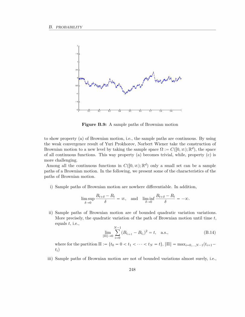
B. PROBABILITY
Figure B.9: A sample paths of Brownian motion
to show property (a) of Brownian motion, i.e., the sample paths are continuous. By usingthe weak convergence result of Yuri Prokhorov, Norbert Wiener take the construction ofBrownian motion to a new level by taking the sample space Ω :“ Cpr0, 8q;Rdq, the spaceof all continuous functions. This way property (a) becomes trivial, while, property (c) ismore challenging.Among all the continuous functions in Cpr0, 8q;Rdq only a small set can be a sample
paths of a Brownian motion. In the following, we present some of the characteristics of thepaths of Brownian motion.
i) Sample paths of Brownian motion are nowhere differentiable. In addition,
lim supδÑ0
Bt`δ ´ Bt
δ“ 8, and lim inf
δÑ0
Bt`δ ´ Bt
δ“ ´8.
ii) Sample paths of Brownian motion are of bounded quadratic variation variations.More precisely, the quadratic variation of the path of Brownian motion until time t,equals t, i.e.,
limΠÑ0
N´1ÿ
i“0pBti`1 ´ Btiq
2 “ t, a.s., (B.14)
where for the partition Π :“ tt0 “ 0 ă t1 ă ¨ ¨ ¨ ă tN “ tu, Π “ maxi“0,...,N´1pti`1´
tiq
iii) Sample paths of Brownian motion are not of bounded variations almost surely, i.e.,
248
C. STOCHASTIC ANALYSIS
for
supΠ
N´1ÿ
i“0|Bti`1 ´ Bti | “ 8, a.s.,
where the supremum is over all partitions Π :“ tt0 “ 0 ă t1 ă ¨ ¨ ¨ ă tN “ tu.
In the above, property (iii) is a result of (ii). More precisely, for a a continuous functiong : ra, bs Ñ R, a nonzero quadratic variation implies infinite bounded variation. To showthis, let’s assume that g is continuous and bounded variation B. Then, g is uniformlycontinuous on ra, bs, i.e., for any ε ą 0, there exists a δ ą 0 such that if Π ď δ, then
maxi“0,...,N´1
t|gpti`1q ´ gptiq|u ď ε.
Thus,
N´1ÿ
i“0pgpti`1q ´ gptiqq2 ď max
i“0,...,N´1t|gpti`1q ´ gptiq|u
N´1ÿ
i“0|gpti`1q ´ gptiq| ď εB.
By sending ε Ñ 0, we obtain that the the quadratic variation vanishes.The following exercise shows the relation between the quadratic variation is martingale
properties of Brownian motion.
Exercise B.25. Show that B2t ´ t is a martingale, i.e.
ErB2t`s ´ pt ` sq | Bss “ B2
s ´ s.
C Stochastic analysisCalculus is the study of derivative (not financial) and integral. Stochastic calculus istherefore the study of integrals and differentials of stochastic objects such as Brownianmotion. In this section, we provide a brief overview of the stochastic integral and Itôformula (stochastic chain rule). The application to finance is provided in Part 3.In calculus, the Riemann integral
şba fptqdt is defined by the limit of Riemann sums:
limδÑ0
δNÿ
i“1fpt˚
i q,
where δ “ b´aN , t0 “ a, ti “ t0 ` iδ, and t˚
i is an arbitrary point in interval rti´1, tis. TheReiman integral can be defined for a limited class of integrands, i.e., the real functions f isRiemann integrable on ra, bs if and only if it is bounded and continuous almost everywhere.A natural extension of Riemann integral is Lebesgue integral, which can be defined on alarge class of real functions, i.e., bounded measurable function on ra, bs.
249

C. STOCHASTIC CALCULUS
A more general form of Riemann integral, Riemann-Stieltjes integral is defined in a similarfashion. For two real functions f, g : ra, bs Ñ R, the integral of the integrand f with respectto integrator g is defined by
ż b
afptqdgptq lim
δÑ0
Nÿ
i“1fpt˚
i qpgptiq ´ gpti´1q.
For Riemann-Stieltjes integral, and its extension, Lebegue-Stieltjes integral, to be well-defined, we need some conditions on f and g.
The condition on the integrand f is similar to the those in Riemann and Lebesgue integrals.For example if f is continuous almost everywhere and at the points of discontinuity of g,then no further condition needs to be imposed on f in the Riemann-Stieltjes integral. Forthe Lebesgue-Stieltjes integral, f only needs to be measurable. However, for g a very crucialcondition is needed to make the integral well-defined. g must be of bounded variation, i.e.
limδÑ0
Nÿ
i“0|gpti`1q ´ gptiq| ă 8.
No matter how nice the function f is, if g is unbounded variation, Riemann-Stieltjes orLebesgue-Stieltjes integral cannot be defined. As seen in Section B.5, the sample paths ofBrownian motion are of unbounded variation, which makes it impossible to use them asthe integrator. Therefore, the integral
şba fptqdBt with respect to Brownian motion cannot
be defined pathwise in the sense of the Riemann-Stitljes or Lebesgue-Stieltjes integrals.In this section, we define a new notion of integral, Itô integral15, which makes sense ofşba fptqdBt in a useful way for some applications, including finance.
One of the major tools in stochastic analysis is the stochastic chain rule. Recall that thechain rule in the differential form is written as dhpgptqq “ g1ptqh1pgptqqdt, which can beused in the change of variable in integral. If vptq “ hpgptqq and h and g are differentiablefunctions, then
ż b
afptqdvptq “
ż b
afptqg1ptqh1pgptqqdt.
The right-hand side above is a Riemann (Lebesgue) integral. As a matter of fact, changeof variable formula for Reimann (Lebesgue) integral is the integral format of the chain rule.For bounded variation but not necessarily differentiable function g, the chain rule in thechange of variable for Riemann-Stieltjes (Lebesgue-Stieltjes) integral can be written in aslightly different way. More precisely, if vptq “ hpgptqq and h is a differentiable function
15Named after Japanese mathematician Kiyosi (read Kiyoshi) Itô, 1915-2008.
250
C. STOCHASTIC CALCULUS
and g is of bounded variation, thenż b
afptqdvptq “
ż b
afptqh1pgptqqdgptq.
In the chain rule for Itô stochastic integral, an extra term appears. If vptq “ hpBtq and his a twice differentiable function, then
ż b
afptqdvptq “
ż b
afptqh1pBtqdBt `
12
ż b
afptqh2pBtqdt.
As expected the termşba fptqh1pBtqdBt shows up like in chain rule. However, the term
12şba fptqh2pBtqdt, which is a simple Riemann integral, is unprecedented. In the remaining
of this section, we provide a heuristic argument why this term should be in the chain rulefor Itô stochastic integral.
C.1 Stochastic integral with respect to Brownian motion and Itô formula
We first introduce a special case of Itô integral, called Wiener integral16. In Wiener integral,we assume that the integrand f is simply a real function and is not stochastic. The thepartial sums
Sδ :“Nÿ
i“1fpti´1qpBti ´ Bti´1q,
is a Gaussian random variable with mean zero and variance
δNÿ
i“1f2pti´1q.
Exercise C.1. Show that Sδ is a Gaussian random variable with mean zero and varianceδřN
i“1 f2pti´1q.Therefore, it follows form
limδÑ0
δNÿ
i“1f2pti´1q “
ż b
af2ptqdt,
that Sδ ñ X where X is a normal random variable with mean zero and varianceşba f2ptqdt.
Notice that in the partial sum for Sδ, we choose ti´1, i.e., the left endpoint on the intervalrti´1, tis. This choice is not crucial to achieve the limit. If we would choose different pointson the interval, we still obtain the same limiting distributions. See Exercise C.2.
16Named after American mathematician Norbert Wiener, 1894-1964.
251
C. STOCHASTIC CALCULUS
Exercise C.2. Calculate that the mean and the variance of partial sums below:a)
řNi“1 fptiqpBti ´ Bti´1q.
b)řN
i“1 f´
ti`ti´12
¯
pBti ´ Bti´1q.
c)řN
i“1 fpti´1qpBti ´ Bti´1q.Then, show that in each case the limit of the calculated quantities as δ Ñ 0 is the same.
Itô integral extends Wiener integral to stochastic integrands. The integrand f is now afunction of time t P ra, bs and ω in sample space Ω. For our analysis in this notes, we onlyneed to define Itô integral on the integrands of the form fpt, Btq where f : ra, bs ˆ R Ñ Ris a measurable function. Similar to the Winer integral we start with the partial sum
N´1ÿ
i“0fpti, BtiqpBti`1 ´ Btiq.
Exercise C.3. Calculate that the mean and the variance of partial sums below:a)
řNi“1 BtipBti ´ Bti´1q.
b)řN
i“1 B ti`ti´12
pBti ´ Bti´1q.
c)řN
i“1 Bti´1pBti ´ Bti´1q.Then, show that in all cases the limits of the calculated quantities as δ Ñ 0 are different.
ż T
0fpu, BuqdBu :“ P ´ lim
δÑ0
N´1ÿ
i“0fpti, BtiqpBti`1 ´ Btiq. (C.1)
The notation P ´ lim means the limit is in probability, i.e., for any ε ą 0,
P
˜
ˇ
ˇ
ˇ
N´1ÿ
i“0fpti, BtiqpBti`1 ´ Btiq ´
ż T
0fpu, BuqdBu
ˇ
ˇ
ˇą ε
¸
Ñ 0 as δ Ñ 0.
The choice of starting point ti in the interval rti, ti`1s in fpti, Btiq is crucial. This is becausechoosing other point in the interval rti, ti`1s leads to different limits. Fo instance,
N´1ÿ
i“0f´ ti ` ti`1
2,Bti`ti`1
2
¯
pBti`1 ´ Btiq
converges toż T
0fpu, BuqdBu `
ż T
0Bxfpu, Buqdu.
252
C. STOCHASTIC CALCULUS
Martingale property of stochastic integral
Consider the discrete sum which converges to the stochastic integral, i.e.
MT :“N´1ÿ
i“0fpti, BtiqpBti`1 ´ Btiq
Assume that the values of B0, ..., Btj are given. We want to evaluate the conditionalexpectation of the stochastic sum MT , i.e.
ErMT | B0, ..., Btj s.
Then, we split the stochastic sum into to parts
MT :“j´1ÿ
i“0fpti, BtiqpBti`1 ´ Btiq `
N´1ÿ
i“j
fpti, BtiqpBti`1 ´ Btiq.
The first summation of the right-hand side above is known given B0, ..., Btj . Thus,
ErMT | B0, ..., Btj s “
j´1ÿ
i“0fpti, BtiqpBti`1 ´ Btiq ` E
«
N´1ÿ
i“j
fpti, BtiqpBti`1 ´ Btiq | B0, ..., Btj
ff
“
j´1ÿ
i“0fpti, BtiqpBti`1 ´ Btiq `
N´1ÿ
i“j
E“
fpti, BtiqpBti`1 ´ Btiq | B0, ..., Btj
‰
Each term in the second summation of right-hand side above can be calculated by towerproperty of conditional expectation
E“
fpti, BtiqpBti`1 ´ Btiq | B0, ..., Btj
‰
“ E“
fpti, BtiqErBti`1 ´ Bti | B0, ..., Btis | B0, ..., Btj
‰
.
Since Bti`1 ´ Bti is independent of B0, ..., Bti ,
ErBti`1 ´ Bti | B0, ..., Btis “ ErBti`1 ´ Btis “ 0.
This implies that the second summation vanishes and we have
ErMT | B0, ..., Btj s “
j´1ÿ
i“0fpti, BtiqpBti`1 ´ Btiq “: Mtj .
In other words, given the Brownian motion up to time tj , the expected values of MT isequal to Mtj . In probability terms, we call this a martingale. By some more technical tools,one can show that given the path of a Brownian motion until time t ă T , the expected
253
C. STOCHASTIC CALCULUS
value of the stochastic integralşT0 fps, BsqdBs is equal to
şt0 fps, BsqdBs, i.e.
E„ż T
0fps, BsqdBs
ˇ
ˇ
ˇ
ˇ
Bs for s P r0, ts
ȷ
“
ż t
0fps, BsqdBs.
One of the consequence of martingale property is that the expectation of stochastic integralis zero, i.e.
E„ż T
0fps, BsqdBs
ȷ
“
ż 0
0fps, BsqdBs “ 0.
Remark C.1. The martingale property of the stochastic integral with respect to Brownianmotion is basically a result of martingale property of Brownian motion. Riemann integralşt0 fps, Bsqds is a martingale if and only if f ” 0. Intuitively, if we assume
şt0 fps, Bsqds is
a martingale, we have
E”
ż t`δ
tfps, Bsqds
ˇ
ˇ
ˇFt
ı
“ 0.
By dividing both sides by δ and then sending δ Ñ 0, we obtain
limδÑ0
E”1
δ
ż t`δ
tfps, Bsqds
ˇ
ˇ
ˇFt
ı
“ Erfpt, Btq | Fts “ fpt, Btq.
C.2 Itô formula
One of the important implications of Itô integral is a very powerful tool called Itô formula.Itô formula is the the stochastic version of Taylor expansion. To understand this betterlet’s try to write Taylor expansion for V pt ` δ, Bt`δq about the point V pt, Btq.
V pt ` δ, Bt`δq “ V pt, Btq ` δBtV pt, Btq ` BxV pt, BtqpBt`δ ´ Btq `12
BxxV pt, BtqpBt`δ ´ Btq2 ` opδq.
(C.2)
The remaining term in of order opδq since Bt`δ ´ Bt „ Op?
δq. Also, we know that
pBt`δ ´ Btq2 ´ δ „ opδq, pBt`δ ´ Btqδ „ opδq, and trivially δ2 „ opδq. (C.3)
If we take conditional expectation with respect to Bt, we obtain
ErV pt ` δ, Bt`δq | Bts “V pt, Btq ` δBtV pt, Btq ` BxV pt, BtqErpBt`δ ´ Btq | Bts
`12
BxxV pt, Btqδ ` opδq.
“V pt, Btq ` pBtV pt, Btq `12
BxxV pt, Btqqδ ` opδq
254
C. STOCHASTIC CALCULUS
Notice that here, by the martingale property of Brownian motion, we have ErpBt`δ ´ Btq |
Bts “ 0. Then, we obtain
ErV pT, BT qs “ V p0, B0q ` E
«
N´1ÿ
i“0pBtV pti, Btiq `
12
BxxV pti, Btiqqδ
ff
` op1q,
which in the limit converges to
ErV pT, BT qs “ V p0, B0q ` E„ż T
0pBtV pti, Btq `
12
BxxV pt, Btqqdt
ȷ
.
The above formula is called Dynkin formula. If we don’t take conditional expectation, wecan write
V pt ` δ, Bt`δq “ V pt, Btq ` pBtV pt, Btq `12
BxxV pt, Btqqδ ` BxV pt, BtqpBt`δ ´ Btq ` opδq.
Then, we obtain
V pT, BT q “ V p0, B0q`
N´1ÿ
i“0pBtV pti, Btiq`
12
BxxV pti, Btiqqδ`
N´1ÿ
i“0BxV pti, BtiqpBti`1´Btiq`op1q.
which in the limit converges to
V pT, BT q “ V p0, B0q `
ż T
0pBtV pt, Btq `
12
BxxV pt, Btqqdt `
ż T
0BxV pt, BtqdBt. (C.4)
In the above, (C.4) is referred to as Itô formula.In a less formal way, Utô formula is given by
dV pt, Btq “ pBtV pt, Btq `12
BxxV pt, Btqqdt ` BxV pt, BtqdBt.
However, it has to be interpreted as (C.4).
Exercise C.4. Use Itô formula to calculate dV pt, Btq in the following cases.
a. V pt, xq “ eax
b. V pt, xq “ e´teax
c. V pt, xq “ e´t cospxq
d. V pt, xq “ e´txa
where a is a given constant.
255

C. STOCHASTIC CALCULUS
C.3 Martingale property of stochastic integral and partial differentialequations
Why martingale property of stochastic integral is important? Recall the Itô formula
dV pt, Btq “ pBtV pt, Btq `12
BxxV pt, Btqqdt ` BxV pt, BtqdBt.
Assume that V pt, xq satisfies the PDE
BtV pt, xq `12
BxxV pt, xq “ 0. (C.5)
Then,dV pt, Btq “ BxV pt, BtqdBt.
and thus V pt, Btq is a martingale, i.e.
V pt, Btq “ ErV pT, BT q | Bs for s P r0, tss.
Conversely, if V pt, Btq is a martingale, then V pt, xq must satisfy the PDE (C.5).
C.4 Stochastic integral and Stochastic differential equation
Riemann integral allows us to write a differential equation dxdt “ fpt, xptqq, xp0q “ x0 as an
integral equation
xptq “ x0 `
ż t
0fps, xpsqqds. (C.6)
Integral equations are more general because the solution does not necessarily need to bedifferentiable. For instance if
fpt, xq “
#
1 t ě 10 t ă 1
.
The solution to the integral equation is xptq “ x0 ` pt ´ 1q`, which is not differentiable att “ 1. While dx “ fpt, xptqqdt should be interpreted as (C.6).Itô integral allows us to define stochastic differential equations (SDE for short) in integral
form. For example, the Black-Scholes differential equation is given by
dSt
St“ rdt ` σdBt.
The true meaning of this term is
St “ S0 ` r
ż t
0Sudu ` σ
ż t
0SudBu.
256
C. STOCHASTIC CALCULUS
The solution is a stochastic process St which satisfies the SDE. In the above case, it is easyto verify, by means of Itô formula, that the geometric Brownian motion
St “ S0 expˆ
pr ´12
σ2qt ` σBt
˙
.
Take V pt, xq “ S0 exp`
pr ´ 12σ2qt ` σx
˘
. It follows from Itô formula that
V pt, Btq “ V p0, B0q `
ż t
0pBtV ps, Bsq `
12
BxxV ps, Bsqqdt `
ż t
0BxV ps, BsqdBs.
Since V p0, xq “ S0, BtV ps, xq “ pr ´ 12σ2qV ps, xq, BxV ps, xq “ σV ps, xq, and BxxV ps, xq “
σ2V ps, xq, we have
V pt, Btq “ S0 ` r
ż t
0V ps, Bsqds ` σ
ż t
0V ps, BsqdBs.
In general for a pair of given functions µpt, xq and σpt, xq, an equation of the form
dSt “ µpt, Stqdt ` σpt, StqdBt (C.7)
is called a stochastic differential equation (SDE). A solution St is a process such that theLebesgue integral
ż t
0µps, Ssqds ă 8 P-a.s.,
the Itô integralż t
0σps, SsqdBs
is well-defined, and the following is satisfied:
St “ S0 `
ż t
0µps, Ssqds `
ż t
0σps, SsqdBs.
For CEV model in Section 3.4.1, SDE is written as
dSt
St“ rdt ` σSβ
t dBt
or in integral form
St “ S0 ` r
ż t
0Sudu ` σ
ż t
0S1`β
u dBu.
One of the most important applications of the Itôs formula is the chain rule in the stochas-
257
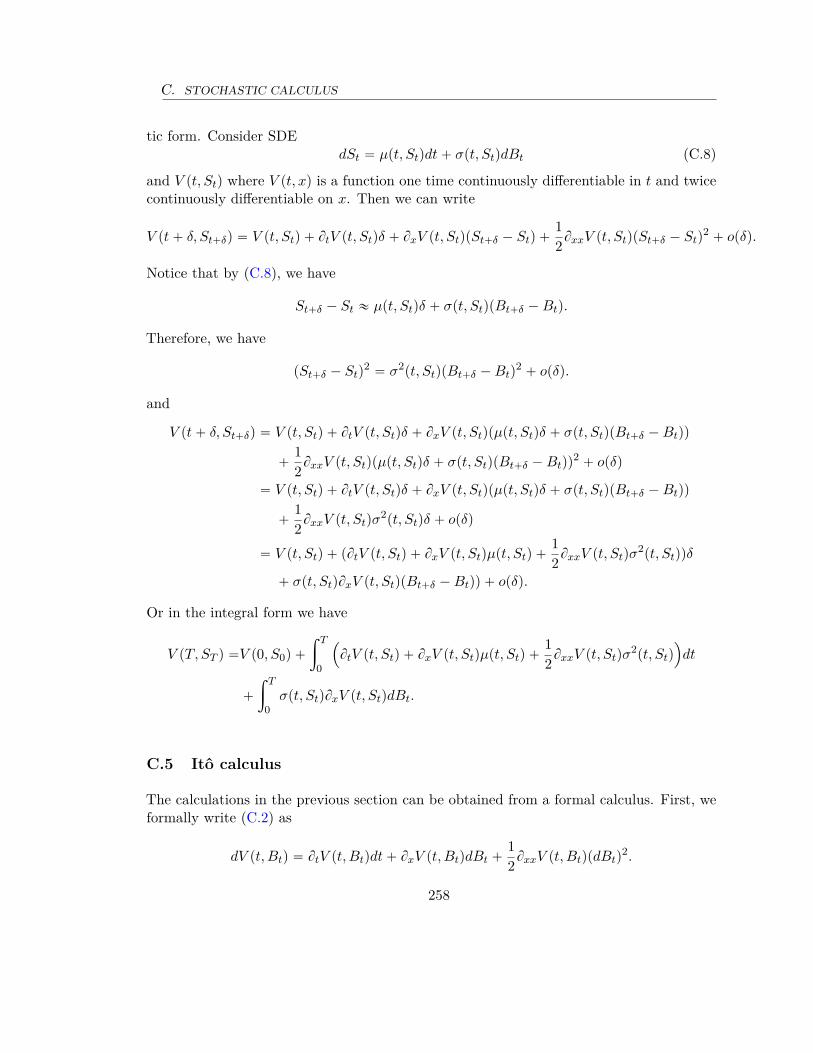
C. STOCHASTIC CALCULUS
tic form. Consider SDEdSt “ µpt, Stqdt ` σpt, StqdBt (C.8)
and V pt, Stq where V pt, xq is a function one time continuously differentiable in t and twicecontinuously differentiable on x. Then we can write
V pt ` δ, St`δq “ V pt, Stq ` BtV pt, Stqδ ` BxV pt, StqpSt`δ ´ Stq `12
BxxV pt, StqpSt`δ ´ Stq2 ` opδq.
Notice that by (C.8), we have
St`δ ´ St « µpt, Stqδ ` σpt, StqpBt`δ ´ Btq.
Therefore, we have
pSt`δ ´ Stq2 “ σ2pt, StqpBt`δ ´ Btq
2 ` opδq.
and
V pt ` δ, St`δq “ V pt, Stq ` BtV pt, Stqδ ` BxV pt, Stqpµpt, Stqδ ` σpt, StqpBt`δ ´ Btqq
`12
BxxV pt, Stqpµpt, Stqδ ` σpt, StqpBt`δ ´ Btqq2 ` opδq
“ V pt, Stq ` BtV pt, Stqδ ` BxV pt, Stqpµpt, Stqδ ` σpt, StqpBt`δ ´ Btqq
`12
BxxV pt, Stqσ2pt, Stqδ ` opδq
“ V pt, Stq ` pBtV pt, Stq ` BxV pt, Stqµpt, Stq `12
BxxV pt, Stqσ2pt, Stqqδ
` σpt, StqBxV pt, StqpBt`δ ´ Btqq ` opδq.
Or in the integral form we have
V pT, ST q “V p0, S0q `
ż T
0
´
BtV pt, Stq ` BxV pt, Stqµpt, Stq `12
BxxV pt, Stqσ2pt, Stq
¯
dt
`
ż T
0σpt, StqBxV pt, StqdBt.
C.5 Itô calculus
The calculations in the previous section can be obtained from a formal calculus. First, weformally write (C.2) as
dV pt, Btq “ BtV pt, Btqdt ` BxV pt, BtqdBt `12
BxxV pt, BtqpdBtq2.
258
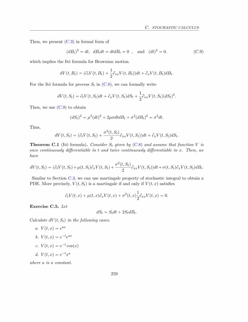
C. STOCHASTIC CALCULUS
Then, we present (C.3) in formal form of
pdBtq2 “ dt, dBtdt “ dtdBt “ 0 , and pdtq2 “ 0. (C.9)
which implies the Itô formula for Brownian motion.
dV pt, Btq “ pBtV pt, Btq `12
BxxV pt, Btqqdt ` BxV pt, BtqdBt.
For the Itô formula for process St in (C.8), we can formally write
dV pt, Stq “ BtV pt, Stqdt ` BxV pt, StqdSt `12
BxxV pt, StqpdStq2.
Then, we use (C.9) to obtain
pdStq2 “ µ2pdtq2 ` 2µσdtdBt ` σ2pdBtq
2 “ σ2dt.
Thus,
dV pt, Stq “ pBtV pt, Stq `σ2pt, Stq
2BxxV pt, Stqqdt ` BxV pt, StqdSt.
Theorem C.1 (Itô formula). Consider St given by (C.8) and assume that function V isonce continuously differentiable in t and twice continuously differentiable in x. Then, wehave
dV pt, Stq “ pBtV pt, Stq`µpt, StqBxV pt, Stq`σ2pt, Stq
2BxxV pt, Stqqdt`σpt, StqBxV pt, StqdBt.
Similar to Section C.3, we can use martingale property of stochastic integral to obtain aPDE. More precisely, V pt, Stq is a martingale if and only if V pt, xq satisfies
BtV pt, xq ` µpt, xqBxV pt, xq ` σ2pt, xq12
BxxV pt, xq “ 0.
Exercise C.5. LetdSt “ Stdt ` 2StdBt.
Calculate dV pt, Stq in the following cases.
a. V pt, xq “ eax
b. V pt, xq “ e´teax
c. V pt, xq “ e´t cospxq
d. V pt, xq “ e´txa
where a is a constant.
259

C. STOCHASTIC CALCULUS
Exercise C.6. In each of the following SDE, find the PDE for the function V pt, xq suchthat V pt, Stq is a martingale.
a. dSt “ σdBt where σ is constants.
b. dSt “ κpm ´ Stqdt ` σdBt where κ, m and σ are constants.
c. dSt “ κpm ´ Stqdt ` σ?
StdBt where κ, m and σ are constants.
d. dSt “ rStdt ` σS2t dBt where r and σ are constants.
Exercise C.7. Consider the SDE
dSt “ rStdt ` σStdBt where r and σ are constants.
a. Find the ODE for the function V pxq such that e´rtV pStq is a martingale.
b. Find all the solutions to the ODE in (a).
260
BIBLIOGRAPHY BIBLIOGRAPHY
Bibliography
[1] M. R. Adams and V. Guillemin, Measure theory and probability, Springer, 1996.
[2] M. Avellaneda and P. Laurence, Quantitative modeling of derivative securities:from theory to practice, CRC Press, 1999.
[3] L. Bachelier, Théorie de la spéculation, Gauthier-Villars, 1900.
[4] D. P. Bertsekas and S. E. Shreve, Stochastic optimal control: the discrete time case,Mathematics in Science and Engineering, Elsevier, Burlington, MA, 1978.
[5] P. Billingsley, Probability and measure, John Wiley & Sons, 2008.
[6] F. Black and M. Scholes, The pricing of options and corporate liabilities, Thejournal of political economy, (1973), pp. 637–654.
[7] B. Bouchard, M. Nutz, et al., Arbitrage and duality in nondominateddiscrete-time models, The Annals of Applied Probability, 25 (2015), pp. 823–859.
[8] B. Bouchard and X. Warin, Monte-carlo valuation of american options: factsand new algorithms to improve existing methods, in Numerical methods in finance,Springer, 2012, pp. 215–255.
[9] S. P. Boyd and L. Vandenberghe, Convex optimization (pdf), Np: CambridgeUP, (2004).
[10] F. Delbaen and W. Schachermayer, A general version of the fundamentaltheorem of asset pricing, Mathematische Annalen, 300 (1994), pp. 463–520.
[11] B. Dupire et al., Pricing with a smile, Risk, 7 (1994), pp. 18–20.
[12] R. Durrett, Probability. theory and examples. the wadsworth & brooks/colestatistics/probability series, Wadsworth & Brooks/Cole Advanced Books & Software,Pacific Grove, CA, (1991).
[13] L. Eisenberg and T. H. Noe, Systemic risk in financial systems, ManagementScience, 47 (2001), pp. 236–249.
261

BIBLIOGRAPHY BIBLIOGRAPHY
[14] A. Fahim, N. Touzi, and X. Warin, A probabilistic numerical method for fullynonlinear parabolic pdes, The Annals of Applied Probability, (2011), pp. 1322–1364.
[15] H. Föllmer and A. Schied, Stochastic finance: an introduction in discrete time,Walter de Gruyter, 2011.
[16] J. Franke, W. K. Härdle, and C. M. Hafner, Statistics of financial markets,vol. 2, Springer, 2004.
[17] P. Glasserman, Monte Carlo methods in financial engineering, vol. 53, SpringerScience & Business Media, 2003.
[18] I. Gyöngy, Mimicking the one-dimensional marginal distributions of processes havingan itô differential, Probability theory and related fields, 71 (1986), pp. 501–516.
[19] J. Hull, Options, Futures and Other Derivatives, Options, Futures and Other Deriva-tives, Pearson/Prentice Hall, 2015.
[20] I. Karatzas and S. Shreve, Brownian motion and stochastic calculus, vol. 113,Springer Science & Business Media, 2012.
[21] P.-S. Laplace, Essai philosophique sur les probabilités, H. Remy, 1829.
[22] F. A. Longstaff and E. S. Schwartz, Valuing american options by simulation: asimple least-squares approach, Review of Financial studies, 14 (2001), pp. 113–147.
[23] H. Markowitz, Portfolio selection, The journal of finance, 7 (1952), pp. 77–91.
[24] R. C. Merton, An analytic derivation of the efficient portfolio frontier, Journal offinancial and quantitative analysis, 7 (1972), pp. 1851–1872.
[25] , Theory of rational option pricing, The Bell Journal of economics and manage-ment science, (1973), pp. 141–183.
[26] B. Oksendal, Stochastic differential equations: an introduction with applications,Springer Science & Business Media, 2013.
[27] G. Peskir and A. Shiryaev, Optimal stopping and free-boundary problems,Springer, 2006.
[28] P. Protter, A partial introduction to financial asset pricing theory, Stochastic pro-cesses and their applications, 91 (2001), pp. 169–203.
[29] R. Rebonato, Volatility and correlation: the perfect hedger and the fox, John Wiley& Sons, 2005.
262

BIBLIOGRAPHY BIBLIOGRAPHY
[30] W. Schachermayer and J. Teichmann, How close are the option pricing formulasof bachelier and black–merton–scholes?, Mathematical Finance, 18 (2008), pp. 155–170.
[31] S. Shreve, Stochastic calculus for finance I: the binomial asset pricing model, SpringerScience & Business Media, 2012.
[32] S. E. Shreve, Stochastic calculus for finance II: Continuous-time models, vol. 11,Springer Science & Business Media, 2004.
[33] M. S. Taqqu, Bachelier and his times: a conversation with bernard bru, Finance andStochastics, 5 (2001), pp. 3–32.
[34] N. Touzi and P. Tankov, No-arbitrage theory for derivative pricing, Cours del’Ecole polytechnique, (2008).
[35] D. Williams, Probability with martingales, Cambridge university press, 1991.
263