introduction to field theory - nihon...
TRANSCRIPT

Appendix A
Introduction to Field Theory
This Appendix is intended for readers who may not be very familiar with the field theoryterminology. In particular, the basic notations which are used in this textbook are explainedin detail. The notation in physics is important since it is just like the language with whichall the communications become possible. Therefore, the notation must be defined well, butreaders should remember them all.
In quantum field theory, the basic concept is, for sure, based on quantum mechanics.Therefore, we explain some of the important ingredients in quantum mechanics. The mostdifficult part of quantum mechanics is the quantization itself, and the quantization procedurewhich is often called thefirst quantizationis consistent with all the experiments even thoughthere is no fundamental principle that may lead to the concept of the quantization. Also, theSchrodinger field is described in terms of the non-relativistic field theory, and apart fromthe kinematics, the behavior of the Schrodinger field from the field theoretical point of viewshould be similar to the relativistic field.
The relativistic quantum mechanics of fermions is described such that readers may un-derstand and remember it all. Apart from the creation and annihilation of particles, theDirac theory can describe physics properly. Some properties of the hydrogen atom areexplained.
The relativistic boson fields are also discussed here. However, we present questionsrather than descriptions of the boson field properties since unfortunately these questionsare not answered well in this textbook. On the other hand, it is by now quite possible thatthe Klein–Gordon equation may not be derived from the fundamental principle any more[82, 62]. These conceptual problems are still not very well organized in this textbook.
Maxwell equation is reviewed here rather in detail from the point of view of the gaugefield theory. In this textbook, the Maxwell equation is considered to be most fundamentalfor all.
Regularization and renormalization are briefly discussed in terms of physical observ-ables. In addition, we describe the path integral formulation since it is an interesting tool.However, it is not very useful for practical calculations, apart from the derivation of Feyn-man diagrams. In this regard, the path integral formulation should be taken as an alternative
191

192 Appendix A. Introduction to Field Theory
tool which is expressed in terms of many dimensional integrals rather than the differentialequations in order to obtain any physical observables.
In Appendix H, we present a new concept of the first quantization itself. Mathemati-cally, there is nothing new in the new picture, but the understanding of quantum mechanicsmay well have a conceptual change in future physics. At least, it should be easy to un-derstand why one can replace the energy and momentum by the differential operators inderiving the Schrodinger equation while there is a good reason to believe that the Klein–Gordon equation for elementary fields cannot be derived from the fundamental principle.
Finally, we review briefly the renormalization scheme in QED. This is well explainedin the standard field theory textbooks, and there is no special need for the presentation ofthe renormalization in QED. Here, we stress that the renormalization in QED itself is wellconstructed since the Fock space of the unperturbed Hamiltonian is prepared in advance.
Notations in Field TheoryIn field theory, one often employs special notations which are by now commonly used.In this Appendix, we explain some of the notations which are particularly useful in fieldtheory.
A.1 Natural Units
In this text, we employ the natural units because of its simplicity
c = 1, h = 1. (A.1.1)
If one wishes to get the right dimensions out, one should use
hc = 197.33 MeV · fm. (A.1.2)
For example, pion mass ismπ ' 140 MeV/c2. Its Compton wave length is
1mπ
=hc
mπc2=
197 MeV · fm140 MeV
' 1.4 fm.
The fine structure constantα is expressed by the coupling constante which is defined insome different ways
α = e2 =e2
hc=
e2
4π=
e2
4πhc=
1137.036
.
Some constants:Electron mass:me = 0.511 MeV/c2
Muon mass:mµ = 105.66 MeV/c2
A.2. Hermite Conjugate and Complex Conjugate 193
Proton mass:Mp = 938.28 MeV/c2
Bohr radius: a0 =1
mee2= 0.529× 10⁻⁸ cm
Magnetic moments:
Electron: µe = 1.00115965219eh
2mec
Theory: µe = 1.0011596524eh
2mec
Muon : µµ = 1.001165920eh
2mµc
.
A.2 Hermite Conjugate and Complex Conjugate
For a complex c-numberAA = a + bi (a, b : real). (A.2.1)
its complex conjugateA∗ is defined as
A∗ = a− bi. (A.2.2)
Matrix A
If A is a matrix, one defines the hermite conjugateA†
(A†)ij = A∗ji. (A.2.3)
Differential Operator A
If A is a differential operator, then the hermite conjugate can be defined only when theHilbert space and its scalar product are defined. For example, supposeA is written as
A = i∂
∂x. (A.2.4)
In this case, its hermite conjugateA† becomes
A† = −i
(∂
∂x
)T
= i∂
∂x= A (A.2.5)
which meansA is Hermitian. This can be easily seen in a concrete fashion since
〈ψ|Aψ〉 =
∞∫
−∞ψ†(x)i
∂
∂xψ(x) dx = −i
∞∫
−∞
(∂
∂xψ†(x)
)ψ(x) dx = 〈Aψ|ψ〉, (A.2.6)
whereψ(±∞) = 0 is assumed. The complex conjugate ofA is simply
A∗ = −i∂
∂x6= A. (A.2.7)

194 Appendix A. Introduction to Field Theory
Field ψ
If the ψ(x) is a c-number field, then the hermite conjugateψ†(x) is just the same as thecomplex conjugateψ∗(x). However, when the fieldψ(x) is quantized, then one shouldalways take the hermite conjugateψ†(x). When one takes the complex conjugate of thefield asψ∗(x), one may examine the time reversal invariance as discussed in Chapter 2.
A.3 Scalar and Vector Products (Three Dimensions) :
Scalar Product
For two vectors in three dimensions
r = (x, y, z) ≡ (x1, x2, x3), p = (px, py, pz) ≡ (p1, p2, p3) (A.3.1)
the scalar product is defined
r · p =3∑
k=1
xkpk ≡ xkpk, (A.3.2)
where, in the last step, we omit the summation notation if the indexk is repeated twice.
Vector Product
The vector product is defined as
r × p ≡ (x2p3 − x3p2, x3p1 − x1p3, x1p2 − x2p1). (A.3.3)
This can be rewritten in terms of components,
(r × p)i = εijkxjpk, (A.3.4)
whereεijk denotes anti-symmetric symbol with
ε123 = ε231 = ε312 = 1, ε132 = ε213 = ε321 = −1, otherwise = 0.
A.4 Scalar Product (Four Dimensions)
For two vectors in four dimensions,
xµ ≡ (t, x, y, z) = (x0, r), pµ ≡ (E, px, py, pz) = (p0, p) (A.4.1)
the scalar product is defined
x · p ≡ Et− r · p = x0p0 − xkpk. (A.4.2)
A.5. Four Dimensional Derivatives∂µ 195
This can be also written as
xµpµ ≡ x0p0 + x1p
1 + x2p2 + x3p
3 = Et− r · p = x · p, (A.4.3)
wherexµ andpµ are defined as
xµ ≡ (x0,−r), pµ ≡ (p0,−p). (A.4.4)
Here, the repeated indices of the Greek letters mean the four dimensional summationµ =0, 1, 2, 3. The repeated indices of the roman letters always denote the three dimensionalsummation throughout the text.
A.4.1 Metric Tensor
It is sometimes convenient to introduce the metric tensorgµν which has the following prop-erties
gµν = gµν =
1 0 0 00 −1 0 00 0 −1 00 0 0 −1
. (A.4.5)
In this case, the scalar product can be rewritten as
x · p = xµpνgµν = Et− r · p. (A.4.6)
A.5 Four Dimensional Derivatives∂µ
The derivative∂µ is introduced for convenience
∂µ ≡ ∂
∂xµ=
(∂
∂x0,
∂
∂x1,
∂
∂x2,
∂
∂x3
)=
(∂
∂t,
∂
∂x,
∂
∂y,
∂
∂z
)=
(∂
∂t, ∇
), (A.5.1)
where the lower index has the positive space part. Therefore, the derivative∂µ becomes
∂µ ≡ ∂
∂xµ=
(∂
∂t,− ∂
∂x,− ∂
∂y,− ∂
∂z
)=
(∂
∂t,−∇
). (A.5.2)
A.5.1 pµ and Differential Operator
Since the operatorpµ becomes a differential operator as
pµ = (E, p) =(
i∂
∂t, −i∇
)= i∂µ
the negative sign, therefore, appears in the space part. For example, if one defines thecurrentjµ in four dimension as
jµ = (ρ, j),
then the current conservation is written as
∂µjµ =∂ρ
∂t+ ∇ · j =
1i
pµjµ = 0. (A.5.3)
196 Appendix A. Introduction to Field Theory
A.5.2 Laplacian and d’Alembertian Operators
The Laplacian and d’Alembertian operators,∆ and2 are defined as
∆ ≡ ∇ ·∇ =∂2
∂x2+
∂2
∂y2+
∂2
∂z2,
2 ≡ ∂µ∂µ =∂2
∂t2−∆.
A.6 γ-Matrices
Here, we present explicit expressions of theγ-matrices in two and four dimensions. Beforepresenting the representation of theγ-matrices, we first give the explicit representation ofPauli matrices.
A.6.1 Pauli Matrices
Pauli matrices are given as
σx = σ1 =(
0 11 0
), σy = σ2 =
(0 −ii 0
), σz = σ3 =
(1 00 −1
). (A.6.1)
Below we write some properties of the Pauli matrices.
Hermiticity
σ†1 = σ1, σ†2 = σ2, σ†3 = σ3.
Complex Conjugate
σ∗1 = σ1, σ∗2 = −σ2, σ∗3 = σ3.
Transposed
σT1 = σ1, σT
2 = −σ2, σT3 = σ3 (σT
k = σ∗k).
Useful Relations
σiσj = δij + iεijkσk, (A.6.2)
[σi, σj ] = 2iεijkσk. (A.6.3)

A.6. γ-Matrices 197
A.6.2 Representation ofγ-matrices
(a) Two dimensional representations ofγ-matrices
Dirac : γ0 =(
1 00 −1
), γ1 =
(0 1−1 0
), γ5 = γ0γ1 =
(0 11 0
),
Chiral : γ0 =(
0 11 0
), γ1 =
(0 −11 0
), γ5 = γ0γ1 =
(1 00 −1
).
(b) Four dimensional representations of gamma matrices
Dirac : γ0 = β =(1 00 −1
), γ =
(0 σ−σ 0
),
γ5 = iγ0γ1γ2γ3 =(0 11 0
), α =
(0 σσ 0
),
Chiral : γ0 = β =(0 11 0
), γ =
(0 −σσ 0
),
γ5 = iγ0γ1γ2γ3 =(1 00 −1
), α =
(σ 00 −σ
).
where 0 ≡(
0 00 0
), 1 ≡
(1 00 1
).
A.6.3 Useful Relations ofγ-Matrices
Here, we summarize some useful relations of theγ-matrices.
Anti-commutation relations
γµ, γν = 2gµν , γ5, γν = 0. (A.6.4)
Hermiticity
ㆵ = γ0γµγ0 (γ†0 = γ0, γ†k = −γk), γ†5 = γ5. (A.6.5)
Complex Conjugate
γ∗0 = γ0, γ∗1 = γ1, γ∗2 = −γ2, γ∗3 = γ3, γ∗5 = γ5. (A.6.6)
Transposed
γTµ = γ0γ
∗µγ0, γT
5 = γ5. (A.6.7)

198 Appendix A. Introduction to Field Theory
A.7 Transformation of State and Operator
When one transforms a quantum state|ψ〉 by a unitary transformationU which satisfies
U †U = 1
one writes the transformed state as
|ψ′〉 = U |ψ〉. (A.7.1)
The unitarity is important since the norm must be conserved, that is,
〈ψ′|ψ′〉 = 〈ψ|U †U |ψ〉 = 1.
In this case, an arbitrary operatorO is transformed as
O′ = UOU−1. (A.7.2)
This can be obtained since the expectation value of the operatorO must be the same be-tween two systems, that is,
〈ψ|O|ψ〉 = 〈ψ′|O′|ψ′〉. (A.7.3)
Since〈ψ′|O′|ψ′〉 = 〈ψ|U †O′U |ψ〉 = 〈ψ|O|ψ〉
one findsU †O′U = O
which is just eq.(A.7.2).
A.8 Fermion Current
We summarize the fermion currents and their properties of the Lorentz transformation. Wealso give their nonrelativistic expressions since the basic behaviors must be kept in thenonrelativistic expressions. Here, the approximate expressions are obtained by making useof the plane wave solutions for the Dirac wave function.
Fermioncurrents :
Scalar : ψψ ' 1
Pseudoscalar : ψγ5ψ ' ·pm
Vector : ψγµψ '(1,
p
m
)
Axialvector : ψγµγ5ψ '(σ · p
m,σ
)
. (A.8.1)
A.9. Trace in Physics 199
Therefore, under the parityP and time reversalT transformation, the above currents behaveas
Parity P :
ψ′ψ′ = ψP−1Pψ = ψψ
ψ′γ5ψ′ = ψP−1γ5Pψ = −ψγ5ψ
ψ′γkψ′ = ψP−1γkPψ = −ψγkψ
ψ′γkγ5ψ′ = ψP−1γkγ5Pψ = ψγkγ5ψ
, (A.8.2)
Timereversal T :
ψ′ψ′ = ψT−1Tψ = ψψ
ψ′γ5ψ′ = ψT−1γ5Tψ = ψγ5ψ
ψ′γkψ′ = ψT−1γkTψ = −ψγkψ
ψ′γkγ5ψ′ = ψT−1γkγ5Tψ = −ψγkγ5ψ
. (A.8.3)
A.9 Trace in Physics
A.9.1 Definition
The trace ofN ×N matrixA is defined as
TrA =N∑
i=1
Aii. (A.9.1)
This is simply the summation of the diagonal elements of the matrixA. It is easy to prove
TrAB = TrBA. (A.9.2)
A.9.2 Trace in Quantum Mechanics
In quantum mechanics, the trace of the HamiltonianH becomes
TrH = TrUHU−1 =∑
n=1
En, (A.9.3)
whereU is a unitary operator that diagonalizes the Hamiltonian, andEn denotes the energyeigenvalue of the Hamiltonian. Therefore, the trace of the Hamiltonian has the meaning ofthe sum of all the eigenvalues of the Hamiltonian.
A.9.3 Trace inSU(N)
In the special unitary groupSU(N), one often describes the elementUa in terms of thegeneratorT a as
Ua = eiT a. (A.9.4)
200 Appendix A. Introduction to Field Theory
In this case, the generator must be hermitian and traceless since
detUa = exp(Tr lnUa) = exp
(iTr T a) = 1 (A.9.5)
and thusTr T a = 0. (A.9.6)
The generators ofSU(N) group satisfy the following commutation relations
[T a, T b] = iCabcT c, (A.9.7)
whereCabc denotes a structure constant in the Lie algebra. The generators are normalizedin this textbook such that
Tr T aT b =12
δab. (A.9.8)
A.9.4 Trace ofγ-Matrices and p/
The Trace of theγ-matrices is also important. First, we have
Tr 1 = 4, Tr γµ = 0, Tr γ5 = 0. (A.9.9)
In field theory, one often defines a symbol ofp/ just for convenience
p/ ≡ pµγµ.
In this case, the following relation holds
p/q/ = pq − iσµνpµqν . (A.9.10)
The following relations may also be useful
Tr p/q/ = 4pq, (A.9.11)
Tr γ5p/q/ = 0, (A.9.12)
Tr p/1p/2p/3p/4 = 4
(p1p2)(p3p4)− (p1p3)(p2p4) + (p1p4)(p2p3)
, (A.9.13)
Tr γ5p/1p/2p/3p/4 = 4iεαβγδ pα1 pβ
2 pγ3 pδ
4. (A.9.14)
Basic Equations and Principles
A.10 Lagrange Equation
In classical field theory, the equation of motion is most important, and it is derived from theLagrange equation. Therefore, we review briefly how we can obtain the equation of motionfrom the Lagrangian density.

A.10. Lagrange Equation 201
A.10.1 Lagrange Equation in Classical Mechanics
Before going to the field theory treatment, we first discuss the Lagrange equation (Newtonequation) in classical mechanics. In order to obtain the Lagrange equation by the variationalprinciple in classical mechanics, one starts from the actionS as defined
S =∫
L(q, q) dt, (A.10.1)
where the LagrangianL(q, q) depends on the general coordinateq and its velocityq. At thetime of deriving equation of motion by the variational principle,q andq are independent asthe function oft. This is clear since, in the actionS, the functional dependence ofq(t) isunknown and therefore one cannot make any derivative ofq(t) with respect to timet. Oncethe equation of motion is established, then one can obtainq by time differentiation ofq(t)which is a solution of the equation of motion.
The Lagrange equation can be obtained by requiring that the actionS should be a min-imum with respect to the variation ofq andq.
δS =∫
δL(q, q) dt =∫ (
∂L
∂qδq +
∂L
∂qδq
)dt
=∫ (
∂L
∂q− d
dt
∂L
∂q
)δq dt = 0, (A.10.2)
where the surface terms are assumed to vanish. Therefore, one obtains the Lagrange equa-tion
∂L
∂q− d
dt
∂L
∂q= 0. (A.10.3)
A.10.2 Hamiltonian in Classical Mechanics
The LagrangianL(q, q) must be invariant under the infinitesimal time displacementε ofq(t) as
q(t + ε) → q(t) + qε, q(t + ε) → q(t) + qε + qdε
dt. (A.10.4)
Therefore, one finds
δL(q, q) = L(q(t + ε), q(t + ε))− L(q, q) =∂L
∂qqε +
∂L
∂qqε +
∂L
∂qqdε
dt= 0. (A.10.5)
Neglecting the surface term, one obtains
δL(q, q) =[∂L
∂qq +
∂L
∂qq − d
dt
(∂L
)]ε =
[d
dt
(L− ∂L
)]ε = 0. (A.10.6)
Thus, if one defines the HamiltonianH as
H ≡ ∂L
∂qq − L (A.10.7)
then it is a conserved quantity.
202 Appendix A. Introduction to Field Theory
A.10.3 Lagrange Equation for Fields
The Lagrange equation for fields can be obtained almost in the same way as the particlecase. For fields, we should start from the Lagrangian densityL and the action is written as
S =∫L
(ψ, ψ,
∂ψ
∂xk
)d3r dt, (A.10.8)
whereψ(x), ψ(x) and ∂ψ∂xk
are independent functional variables.The Lagrange equation can be obtained by requiring that the actionS should be a min-
imum with respect to the variation ofψ, ψ and ∂ψ∂xk
,
δS =∫
δL(
ψ, ψ,∂ψ
∂xk
)d3r dt =
∫ (∂L∂ψ
δψ +∂L∂ψ
δψ +∂L
∂( ∂ψ∂xk
)δ
(∂ψ
∂xk
))d3r dt
=∫ (
∂L∂ψ
− ∂
∂t
∂L∂ψ
− ∂
∂xk
∂L∂( ∂ψ
∂xk)
)δψ d3r dt = 0, (A.10.9)
where the surface terms are assumed to vanish. Therefore, one obtains
∂L∂ψ
=∂
∂t
∂L∂ψ
+∂
∂xk
∂L∂( ∂ψ
∂xk), (A.10.10)
which can be expressed in the relativistic covariant way as
∂L∂ψ
= ∂µ
(∂L
∂(∂µψ)
). (A.10.11)
This is the Lagrange equation for fieldψ, which should hold for any independent fieldψ.
A.11 Noether Current
If the Lagrangian density is invariant under the transformation of the field with a continuousvariable, then there is always a conserved current associated with this symmetry. This iscalledNoether currentand can be derived from the invariance of the Lagrangian densityand the Lagrange equation.
A.11.1 Global Gauge Symmetry
The Lagrangian density which is discussed in this textbook should have the following func-tional dependence in general
L = iψγµ∂µψ −mψψ + LI
[ψψ, ψγ5ψ, ψγµψ
].
A.11. Noether Current 203
This Lagrangian density is obviously invariant under the global gauge transformation
ψ′ = eiαψ, ψ′† = e−iαψ†, (A.11.1)
whereα ia a real constant. Therefore, the Noether current is conserved in this system.To derive the Noether current conservation for the global gauge transformation, one canconsider the infinitesimal global transformation, that is,|α| ¿ 1. In this case, the transfor-mation becomes
ψ′ = ψ + δψ, δψ = iαψ. (A.11.2a)
ψ′† = ψ† + δψ†, δψ† = −iαψ†. (A.11.2b)
Invariance of Lagrangian Density
Now, it is easy to find
δL = L(ψ′, ψ′†, ∂µψ′, ∂µψ′†)− L(ψ, ψ†, ∂µψ, ∂µψ†) = 0. (A.11.3a)
At the same time, one can easily evaluateδL
δL =∂L∂ψ
δψ +∂L
∂(∂µψ)δ (∂µψ) +
∂L∂ψ†
δψ† +∂L
∂(∂µψ†)δ(∂µψ†
)
= iα
[(∂µ
∂L∂(∂µψ)
)ψ +
∂L∂(∂µψ)
∂µψ −(
∂µ∂L
∂(∂µψ†)
)ψ† − ∂L
∂(∂µψ†)∂µψ†
]
= iα∂µ
[∂L
∂(∂µψ)ψ − ∂L
∂(∂µψ†)ψ†
]= 0, (A.11.3b)
where the equation of motion forψ is employed.
Current Conservation
Therefore, if one defines the currentjµ as
jµ ≡ −i
[∂L
∂(∂µψ)ψ − ∂L
∂(∂µψ†)ψ†
](A.11.4)
then one has∂µjµ = 0. (A.11.5)
For Dirac fields with electromagnetic interactions or self-interactions, one can obtain as aconserved current
jµ = ψγµψ. (A.11.6)

204 Appendix A. Introduction to Field Theory
A.11.2 Chiral Symmetry
When the Lagrangian density is invariant under the chiral transformation,
ψ′ = eiαγ5ψ (A.11.7)
then there is another Noether current. Here,δψ as defined in eq.(A.11.2) becomes
δψ = iαγ5ψ. (A.11.8)
Therefore, a corresponding conserved current for massless Dirac fields with electromag-netic interactions or self-interactions can be obtained
jµ5 = −i
∂L∂(∂µψ)
γ5ψ = ψγµγ5ψ. (A.11.9)
In this case, we have∂µjµ
5 = 0 (A.11.10)
which is the conservation of the axial vector current. The conservation of the axial vectorcurrent is realized for field theory models with massless fermions.
A.12 Hamiltonian Density
The Hamiltonian densityH is constructed from the Lagrangian densityL. The field theorymodels which we consider should possess the translational invariance. If the Lagrangiandensity is invariant under the translationaµ, then there is a conserved quantity which is theenergy momentum tensorT µν . The Hamiltonian density is constructed from the energymomentum tensor ofT 00.
A.12.1 Hamiltonian Density from Energy Momentum Tensor
Now, the Lagrangian density is given asL(ψi, ψi,
∂ψi∂xk
). If one considers the following
infinitesimal translationaµ of the fieldψi andψ†i
ψ′i = ψi + δψi, δψi = (∂νψi)aν ,
ψ†i′= ψ†i + δψ†i , δψ†i = (∂νψ
†i )a
ν ,
then the Lagrangian density should be invariant
δL ≡ L(ψ′i, ∂µψ′i)− L(ψi, ∂µψi)
=∑
i
[∂L∂ψi
δψi +∂L
∂(∂µψi)δ(∂µψi) +
∂L∂ψ†i
δψ†i +∂L
∂(∂µψ†i )δ(∂µψ†i )
]= 0. (A.12.1)

A.12. Hamiltonian Density 205
Making use of the Lagrange equation, one obtains
δL =∑
i
[∂L∂ψi
(∂νψi) +∂L
∂(∂µψi)(∂µ∂νψi)− ∂µ
(∂L
∂(∂µψi)∂νψi
)]aν
+∑
i
[∂L∂ψ†i
(∂νψ†i ) +
∂L∂(∂µψ†i )
(∂µ∂νψ†i )− ∂µ
(∂L
∂(∂µψ†i )∂νψ
†i
)]aν
= ∂µ
[Lgµν −
∑
i
(∂L
∂(∂µψi)∂νψi +
∂L∂(∂µψ†i )
∂νψ†i
)]aν = 0. (A.12.2)
Energy Momentum TensorT µν
Therefore, if one defines the energy momentum tensorT µν by
T µν ≡∑
i
(∂L
∂(∂µψi)∂νψi +
∂L∂(∂µψ†i )
∂νψ†i
)− Lgµν (A.12.3)
thenT µν is a conserved quantity, that is
∂µT µν = 0.
This leads to the definition of the Hamltonian densityH in terms ofT 00
H ≡ T 00 =∑
i
(∂L
∂(∂0ψi)∂0ψi +
∂L∂(∂0ψ
†i )
∂0ψ†i
)− L. (A.12.4)
A.12.2 Hamiltonian Density from Conjugate Fields
When the Lagrangian density is given asL(ψi, ψi,∂ψi
∂xk), one can define the conjugate fields
Πψi andΠψ†i
as
Πψi ≡∂L∂ψi
, Πψ†i≡ ∂L
∂ψ†i.
In this case, the Hamiltonian density can be written as being consistent with eq.(A.12.4)
H =∑
i
(Πψiψi + Π
ψ†iψ†i
)− L. (A.12.5)
It should be noted that this way of making the Hamiltonian density is indeed easier toremember than the construction starting from the energy momentum tensor.

206 Appendix A. Introduction to Field Theory
Hamiltonian
The Hamiltonian is defined by integrating the Hamiltoian density over all space
H =∫H d3r =
∫ [∑
i
(Πψiψi + Πψ†i
ψ†i )− L]
d3r.
A.12.3 Hamiltonian Density for Free Dirac Fields
For a free Dirac field with its massm, the Lagrangian density becomes
L = ψ†i ψi + ψ†i [iγ0γ ·∇−mγ0]ij ψj .
Therefore, the conjugate fieldsΠψi andΠψ†i
are obtained
Πψi ≡∂L∂ψi
= ψ†i , Πψ†i
= 0.
Thus, the Hamiltonian density becomes
H=∑
i
(Πψi
ψi+Πψ†i
ψ†i)−L= ψi [−iγk∂k+m]ij ψj = ψ [−iγ ·∇+m] ψ. (A.12.6)
A.12.4 Hamiltonian for Free Dirac Fields
The HamiltonianH is obtained by integrating the Hamiltonian density over all space andthus can be written as
H =∫H d3r =
∫ψ [−iγ ·∇ + m] ψ d3r. (A.12.7)
In classical field theory, this Hamiltonian is not an operator but is just the field energy itself.However, this field energy cannot be evaluated unless one knows the shape of the fieldψ(x) itself. Therefore, one should determine the shape of the fieldψ(x) by the equation ofmotion in the classical field theory.
A.12.5 Role of Hamiltonian
We should comment on the usefulness of the classical field Hamiltonian itself for fieldtheory models. In fact, the Hamiltonian alone is not useful. This is similar to the classicalmechanics case in which the Hamiltonian of a point particle itself does not tell a lot. Instead,one has to derive the Hamilton equations in order to calculate some physical properties ofthe system and the Hamilton equations are equivalent to the Lagrange equations in classicalmechanics.

A.12. Hamiltonian Density 207
Classical Field Theory
In classical field theory, the situation is just the same as the classical mechanics case. Ifone stays in the classical field theory, then one should derive the field equation from theHamiltonian by the functional variational principle as will be discussed in the next section.
Quantized Field Theory
The Hamiltonian of the field theory becomes important when the fields are quantized. Inthis case, the Hamiltonian becomes an operator, and thus one has to solve the eigenvalueproblem for the quantized HamiltonianH
H|Ψ〉 = E|Ψ〉, (A.12.8)
where|Ψ〉 is calledFock stateand should be written in terms of the creation and annihilationoperators of fermion and anti-fermion. The space spanned by the Fock states is calledFockspace.
In normal circumstances of the field theory models such as QED and QCD, it is prac-tically impossible to find the eigenstate of the quantized Hamiltonian. The difficulty of thequantized field theory comes mainly from two reasons. Firstly, one has to construct thevacuum state which is composed of infinite many negative energy particles interacting witheach other. The vacuum state should be the eigenstate of the Hamiltonian
H|Ω〉 = EΩ|Ω〉,whereEΩ denotes the energy of the vacuum and it is in general infinity with the negativesign. The vacuum state|Ω〉 is composed of infinitely many negative energy particles
|Ω〉 =∏p,s
b†(s)p |0〉〉,
where|0〉〉 denotes the null vacuum state. In the realistic calculations, the number of thenegative energy particles must be set to a finite value, and this should be reasonable sincephysical observables should not depend on the properties of the deep negative energy parti-cles. However, it is most likely that the number of the negative energy particles should be,at least, larger than a few thousand for two dimensional field theory models.
The second difficulty arises from the operators in the Hamiltonian which can change thefermion and anti-fermion numbers and therefore can induce infinite series of the transitionsamong the Fock states. Since the spectrum of bosons and baryons can be obtained byoperating the fermion and anti-fermion creation operators on the vacuum state, the Fockspace which is spanned by the creation and annihilation operators becomes infinite. Inthe realistic calculations, the truncation of the Fock space becomes most important, eventhough it is difficult to find any reasonable truncation scheme.
In this respect, the Thirring model is an exceptional case where the exact eigenstate ofthe quantized Hamiltonian is found. This is, however, understandable since the Thirringmodel Hamiltonian does not contain the operators which can change the fermion and anti-fermion numbers.

208 Appendix A. Introduction to Field Theory
A.13 Variational Principle in Hamiltonian
When one has the Hamiltonian, then one can derive the equation of motion by requiringthat the Hamiltonian should be minimized with respect to the functional variation of thestateψ(r).
A.13.1 Schrodinger Field
When one minimizes the Hamiltonian
H =∫ [
− 12m
ψ†∇2ψ + ψ†Uψ
]d3r (A.13.1)
with respect toψ(r), then one can obtain the static Schrodinger equation.
Functional Derivative
First, one defines the functional derivative for an arbitrary functionψi(r) by
δψi(r′)δψj(r)
= δijδ(r − r′). (A.13.2)
This is the most important equation for the functional derivative, and once one accepts thisdefinition of the functional derivative, then one can evaluate the functional variation just inthe same way as normal derivative of the functionψi(r).
Functional Variation of Hamiltonian
For the condition onψ(r), one requires that it should be normalized according to∫
ψ†(r)ψ(r) d3r = 1. (A.13.3)
In order to minimize the Hamiltonian with the above condition, one can make use of theLagrange multiplier and make a functional derivative of the following quantity with respectto ψ†(r)
H[ψ] =∫ [
− 12m
ψ†(r′)∇02ψ(r′) + ψ†(r′)Uψ(r′)]
d3r′
−E
(∫ψ†(r′)ψ(r′) d3r′ − 1
), (A.13.4)
whereE denotes a Lagrange multiplier and just a constant. In this case, one obtains
δH[ψ]δψ†(r)
=∫
δ(r − r′)[− 1
2m∇02ψ(r′) + Uψ(r′)−Eψ(r′)
]d3r′ = 0. (A.13.5)
Therefore, one finds
− 12m
∇2ψ(r) + Uψ(r) = Eψ(r) (A.13.6)
which is just the static Schrodinger equation.

A.13. Variational Principle in Hamiltonian 209
A.13.2 Dirac Field
The Dirac equation for free field can be obtained by the variational principle of the Hamil-tonian eq.(A.12.7). Below, we derive the static Dirac equation in a concrete fashion by thefunctional variation of the Hamiltonian.
Functional Variation of Hamiltonian
For the condition onψi(r), one requires that it should be normalized according to∫
ψ†i (r)(γ0)ijψj(r) d3r = 1. (A.13.7)
Now, the Hamiltonian should be minimized with the condition of eq.(A.13.7)
H[ψi] =∫
ψ†i (r)[−i(γ0γ ·∇)ij + m(γ0)ij
]ψj(r) d3r
−E
(∫ψ†i (r)(γ0)ijψj(r) d3r − 1
), (A.13.8)
whereE is just a constant of the Lagrange multiplier. By minimizing the Hamiltonian withrespect toψ†i (r), one obtains
(−iγ ·∇ + m) ψ(r)− Eψ(r) = 0 (A.13.9)
which is just the static Dirac equation for free field.


Appendix B
Non-relativistic Quantum Mechanics
The quantization has two kinds of the procedure, the first quantization and the second quan-tization. By the first quantization, we mean that the coordinater and the momentump of apoint particle do not commute with each other. That is,
[xi, pj ] = ihδij .
In terms of this quantization procedure, we can obtain the Schrodinger equation by requiringthat the particle Hamiltonian should be an operator and therefore the stateψ should beintroduced.
There is another quantization procedure, the second quantization, which is the quantiza-tion of fields. From the experimental observations of creations and annihilations of particlepairs or photons, one needs to quantize fields. The field quantization is closely connected tothe relativistic field equations which inevitably includes anti-particle states (negative energystates in fermion field case). In this respect, one does not have to quantize the Schrodingerfield in the non-relativistic quantum mechanics. Therefore, we discuss only the first quan-tization procedure and problems related to the quantization.
B.1 Procedure of First Quantization
In the standard procedure of the first quantization, the energyE and momentump areregarded as operators, and the simplest expressions ofE andp are given as
E → i∂
∂t, p → −i∇. (B.1.1)
For a free point particle with its massm, the dispersion relation can be written as
E =p2
2m. (B.1.2)
If one employs the quantization procedure of eq.(B.1.1), then one should prepare somestate which receives the operation of eq.(B.1.1). This state is called wave function and is
211

212 Appendix B. Non-relativistic Quantum Mechanics
often denoted asψ(r, t). In this case, eq.(B.1.2) becomes
i∂
∂tψ(r, t) = − 1
2m∇2ψ(r, t) (B.1.3)
which is the Schrodinger equation.
New Picture of First Quantization
At a glance, one may feel that the procedure of eqs.(B.1.1) and (B.1.2) are more fundamen-tal than eq.(B.1.3) itself. However, this is not so trivial. If one looks into the Maxwell equa-tion, then one realizes that the Maxwell equation is already a quantized equation for classi-cal electromagnetic fields. In this respect, the Maxwell equation does not have any corre-sponding classical equation of motions like the Newton equation. In this sense, eq.(B.1.3)can be regarded as a fundamental equation for quantum mechanics as well, even though onecan derive eq.(B.1.3) from eqs.(B.1.1) and (B.1.2).
In fact, in Appendix H, we treat the derivation of the Dirac equation from the Maxwellequation and the local gauge invariance, and there we see that the first quantization ofeq.(B.1.1) is not needed and therefore it is not the fundamental principle any more. Instead,the Schrodinger equation is obtained from the non-relativistic reduction of the Dirac equa-tion. In this respect, the derivation of the Schrodinger equation does not involve the firstquantization.
B.2 Mystery of Quantization or Hermiticity Problem?
Here, we present a problem related to the quantization in box with the periodic bound-ary conditions. We restrict ourselves to the one dimensional case, but the result is easilygeneralized to three dimensions.
B.2.1 Free Particle in Box
By denoting the wave function as
ψ(x) = e−iEtu(x)
the static Schrodinger equation without interactions is written
− 12m
∂2u(x)∂x2
= Eu(x). (B.2.1)
The solution can be obtained as
u(x) =
1√L
eikx,1√L
e−ikx
, with E =
k2
2m, (B.2.2)
B.2. Mystery of Quantization or Hermiticity Problem? 213
where one puts the particle into a box with its lengthL. Now, one requires that the wavefunctionu(x) should satisfy the periodic boundary conditions and should be the eigenstateof the momentum. In this case, one has
puk(x) = kuk(x), k =2πn
L, n = 0,±1, . . . .
Therefore, one can write the eigenstate wave function as
un(x) =1√L
ei 2πnL
x, n = 0,±1, . . . .
B.2.2 Hermiticity Problem
Now, the quantization relation is written
px− xp = −i (B.2.3)
and one takes the expectation value of the quantization relation with the wave functionun(x) and obtains
〈un|px− xp|um〉 = −iδnm. (B.2.4)
If one makes use of the hermiticity ofp, then one obtains
(n−m)2π
L〈un|x|um〉 = −iδnm. (B.2.5)
However, the above equation does not hold forn = m since the left hand side is zero whilethe right hand side is−i.
What is wrong with the calculation? The answer is simple, and one should not makeuse of the hermiticity of the momentump because the surface term at the boundary doesnot vanish for the periodic boundary condition. In fact, in the above evaluation, the surfaceterm just gives the missing constant of−i for n = m. In other words, one can easily showthe following equation
〈un|px|un〉 = −i + 〈pun|x|un〉. (B.2.6)
It should be noted that the hermiticity of the momentum in the following sense is valid
〈un|p|um〉 = 〈pun|um〉. (B.2.7)
From this exercise, one learns that the quantization condition of eq.(B.2.3) should be allright, but the hermiticity of the momentum operator cannot necessarily be justified as longas one employs the periodic boundary conditions for the wave functions. Also, the periodicboundary conditions must be physically acceptable. Therefore, one should be careful fortreating the momentum operator and it should be operated always on the right hand side asit is originally meant. In this case, one does not make any mistakes.
This argument must be valid even for a very largeL as long as one keeps the periodicboundary conditions. This may look slightly odd, but the free particle should be present

214 Appendix B. Non-relativistic Quantum Mechanics
anywhere in the physical space, and therefore one should give up the vanishing of thesurface term in the plane wave case. The criteria of right physics must be given fromthe observation that physical observables should not depend onL. In other words, oneshould take the value ofL much larger than any other scales in the model, and this is calledthermodynamic limit. In order to obtain any physical observables, one should always takethe thermodynamic limit.
B.3 Schrodinger Fields
The Schrodinger equation with a potentialU(r) is written as
i∂ψ(r, t)
∂t=
(− 1
2m∇2 + U(r)
)ψ(r, t). (B.3.1)
From this equation, one can derive the vector current conservation
∂ρ
∂t+ ∇ · j = 0, (B.3.2)
whereρ andj are defined as
ρ = ψ†ψ, j = − i
2m
(ψ†∇ψ − (∇ψ†)ψ
). (B.3.3)
B.3.1 Currents of Bound State
Now, it is interesting to observe how the currents from this Schrodinger field behave inthe realistic physical situations. Since the time dependence of the Schrodinger fieldψ isfactorized as
ψ(r, t) = e−iEtu(r)
the basic properties of the field are represented by the fieldu(r). When the fieldu(r)represents a bound state, thenu(r) becomes a real field. In this case, the current densityjvanishes to zero,
j = − i
2m
(u(r)∇u(r)− (∇u(r))u(r)
)= 0. (B.3.4)
On the other hand, the probability density ofρ ≡ |u(r)|2 is always time-independent, andsince the bound state wave function is confined within a limited area of space, theρ is alsolimited within some area of space.
B.3.2 Free Fields (Static)
When there is no potential, that isU(r) = 0
B.3. Schrodinger Fields 215
then the field can be described as a free particle solution. This solution is obtained whenthe theory is put into a box with its volumeV ,
ψ(r, t) =1√V
e−iEteik·r,1√V
e−iEte−ik·r, (B.3.5)
whereE is the energy of the particle andk denotes a quantum number which should cor-respond to the momentum of a particle. In this case, the probability density is finite andconstant
ρ =1V
(B.3.6)
while the currentj is also a constant and can be written as
j =k
m(B.3.7)
which just corresponds to the velocity of a particle.
Real Field Condition
It is important to note that the Schrodinger fieldψ should be a complex function. If oneimposes the condition that the field should be real,
ψ(r, t) = ψ†(r, t)
then one obtains from the Schrodinger equation eq.(B.1.3)
∂ψ(r, t)∂t
= 0.
Therefore, the Schrodinger fieldψ should be time independent. In this case, one sees im-mediately that the energyE must be zero since
(− 1
2m∇2 + U(r)
)ψ(r, t) = 0.
Therefore, the real field condition ofψ is too strong and it should not be imposed beforesolving the Schrodinger equation. This concept should always hold in the Schrodinger field,and therefore it is most likely true that the same concept should hold for relativistic bosonfields as well. However, this statement may not be justified if the Klein–Gordon field shouldnot have any correspondence with the Schrodinger field in the non-relativistic limit.
B.3.3 Degree of Freedom of Schrodinger Field
The Schrodinger field is a complex field. However, the Schrodinger fieldψ itself shouldcorrespond to one particle. It is clear that one cannot make the following separation of thefield into real and imaginary parts
ψ(r, t) = ρ(r, t)eiξ(r,t) (B.3.8)
216 Appendix B. Non-relativistic Quantum Mechanics
and claim thatρ(r, t) andξ(r, t) describe two independent fields (particles). Whenψ is acomplex field, it has right properties as a field, and the current density of theψ field has afinite value.
B.4 Hydrogen-like Atoms
When the potentialU(r) is a Coulomb type,
U(r) = −Ze2
r(B.4.1)
then the Schrodinger equation can be solved exactly and the Schrodinger fieldψ togetherwith the energy eigenvalueE can be obtained as
ψ(r) = Rn`(r)Y`m(θ, ϕ), (B.4.2)
En = −mZ2e4
2n2= − m
2n2
(Z
137
)2
, (B.4.3)
whereRn`(r) andY`m denote the radial wave function and the spherical harmonics, re-spectively. The principal quantum numbern runs asn = 1, 2, . . . ,∞, and ` runs as` = 0, 1, 2, . . . ,∞, satisfying the condition
` ≤ n− 1. (B.4.4)
It should be worth writing the explicit shape of the wave functions for a few lowest statesof 1s, 2p and2s with the Bohr radiusa0 = 1
me2 .
1s−statee : R1s(r) =(
Z
a0
) 32
2e−Zr
a0 , Y00(θ, ϕ) =1√4π
,
2p−state : R2p(r) =(
Z
2a0
) 32 Zr√
3 a0
e− Zr
2a0 ,
Y11(θ, ϕ) = −√
38π
sin θeiϕ
Y10(θ, ϕ) =
√34π
cos θ
Y1−1(θ, ϕ) =
√38π
sin θe−iϕ
,
2s−state : R2s(r) =1
2√
2
(Z
a0
) 32(
2− Zr
a0
)e− Zr
2a0 , Y00(θ, ϕ) =1√4π
.
B.5. Harmonic Oscillator Potential 217
B.5 Harmonic Oscillator Potential
The harmonic oscillator potentialU(x)
U(x) =12
mω2x2
is a very special potential which is often used in quantum mechanics exercise problemssince the Schrodinger equation with the harmonic oscillator potential can be solved exactly.However, the harmonic oscillator potential is not realistic since it does not have a free field-like solution. The Schrodinger field in the harmonic oscillator potential is always confinedand there is no scattering state solution.
Nevertheless, it should be worth writing solutions of the Schrodinger fieldψ with itsmassm in the one dimensional harmonic oscillator potential. The Schrodinger equationcan be written as (
− 12m
∂2
∂x2+
12
mω2x2
)ψ(x) = Eψ(x). (B.5.1)
In this case, the solution of the Schrodinger fieldψ together with the energy eigenvalueEcan be obtained as
ψn(x) =(
α2
4nπ(n!)2
) 14
Hn(αx)e−12α2x2
, (B.5.2a)
En = ω
(n +
12
), n = 0, 1, 2, . . . , (B.5.2b)
whereα is given as
α =√
mω . (B.5.3)
Hn(ξ) denotes the hermite polynomial and is given as
Hn(ξ) = (−)neξ2 dn
dξne−ξ2
sinceHn(ξ) can be expressed in terms of the generating function as
e−x2+2ξx = e−(x−ξ)2+ξ2=
∞∑
n=0
1n!
Hn(ξ)xn.
Some of them are given below
H0(ξ) = 1, H1(ξ) = 2ξ, H2(ξ) = 4ξ2 − 2, (B.5.4a)
H3(ξ) = 8ξ3 − 12ξ, H4(ξ) = 16ξ4 − 48ξ2 + 12. (B.5.4b)
218 Appendix B. Non-relativistic Quantum Mechanics
B.5.1 Creation and Annihilation Operators
The Hamiltonian of the one dimensional harmonic oscillator potential
H =p2
2m+
12
mω2x2 (B.5.5)
can be rewritten in terms of creationa† and annihilationa operators
a† =√
mω
2x− i√
2mωp, a =
√mω
2x +
i√2mω
p (B.5.6)
as
H = ω
(a†a +
12
). (B.5.7)
a† anda satisfies the following commutation relation
[a, a†] = 1 (B.5.8)
because of the definition ofa† anda in eq.(B.5.6).
Number Operator N
By introducing the number operatorN as
N = a†a (B.5.9)
one finds[N , a] = −a, [N , a†] = a†. (B.5.10)
With the eigenstate|φn〉 of the number operatorN and its eigenvaluen
N |φn〉 = n|φn〉 (B.5.11)
one can easily prove the following equations
a†|φn〉 =√
n + 1 |φn+1〉, a|φn〉 =√
n |φn−1〉. (B.5.12)
This indicates thata† operator increases the quantum numbern by one unit whilea de-creases it in the same way. Therefore,a† anda are calledcreationandannihilation op-erators, respectively. In addition, one can evaluate the expectation value of the numberoperatorN with the state|φn〉 as
n = 〈φn|a†a|φn〉 = ‖aφn‖2 ≥ 0
which shows that then must be a non-negative value. Therefore, one finds from eq.(B.5.12)
a|φ0〉 = 0. (B.5.13)
B.5. Harmonic Oscillator Potential 219
Therefore, one sees that the smallest value ofn is n = 0. This leads to the constraint forn as
n = 0, 1, 2, . . . . (B.5.14)
Operating the HamiltonianH on |φn〉, one finds
H|φn〉 = ω
(N +
12
)|φn〉 = ω
(n +
12
)|φn〉 = En|φn〉. (B.5.15)
Thus, the energyEn can be written as
En = ω
(n +
12
), n = 0, 1, 2, . . .
which agrees with the result given in eq.(B.5.2). The state|φn〉 can be easily constructedby operatinga† operator onto the|φ0〉
|φn〉 =1√n!
(a†
)n|φ0〉. (B.5.16)
It should be noted that the state|φn〉 is specified by the quantum numbern. If one wishesto obtain an explicit expression of the wave function, then one should project the state|φn〉onto the|x〉 or |p〉 representation as given below.
Explicit Wave Function in x-representation
The wave functionψn(x) ≡ 〈x|φn〉 in thex-representation can be obtained in the followingway. First, one solves the differential equation from eq.(B.5.13)
〈x|a|x〉〈x|φ0〉 =(√
mω
2x +
1√2mω
∂
∂x
)ψ0(x) = 0 (B.5.17)
which leads to the ground state wave function
ψ0(x) =(
α2
π
) 14
e−12α2x2
, with α =√
mω. (B.5.18)
From eq.(B.5.16), one obtains the wave function for an arbitrary stateψn(x)
ψn(x) =1√n!〈x|
(a†
)n|x〉〈x|φ0〉
=1√n!
(α2
π
) 14(√
mω
2x− 1√
2mω
∂
∂x
)n
e−12
α2x2
which can be shown to be just identical to eq.(B.5.2a).

Appendix C
Relativistic Quantum Mechanics ofBosons
When a particle motion becomes comparable to the velocity of light, then one has to con-sider the relativistic effects. The dispersion relation between the energy and momentum ofthe particle with its massm becomes
E =√
p2 + m2 . (C.0.1)
If one employs the quantization procedure of eq.(B.1.1),
E → i∂
∂t, p → −i∇
then one obtains the following equation from eq.(C.0.1)
i∂
∂tφ =
√−∇2 + m2 φ. (C.0.2)
However, it is easy to realize that the differential operator in square root cannot be definedwell.
C.1 Klein–Gordon Equation
Therefore, it is essential to rewrite eq.(C.0.1) for the quantization procedure
E2 = p2 + m2. (C.1.1)
From this dispersion relation, one obtains
(∂2
∂t2−∇2 + m2
)φ = 0 (C.1.2)
221

222 Appendix C. Relativistic Quantum Mechanics of Bosons
which is the Klein–Gordon equation. Eq.(C.1.2) can describe bosons which must be aspinless particle. This is clear since the fieldφ has only one component, and therefore itshould correspond to one component particle which is the spin zero state.
It should be interesting to compare eq.(C.1.2) with the equation for the electromagneticfield eq.(E.5.1) which is the resulting equation from the Maxwell equation. One sees thatthe Maxwell equation has just the same structure as the Klein–Gordon equation. In thisrespect, the Maxwell equation does correspond already to the relativistic quantum mechan-ics. Indeed, in Appendix H, we will see that the Dirac equation can be obtained from theassumption that the Maxwell equation and the local gauge invariance are the most funda-mental principles. In this case, one sees that the Klein–Gordon equation cannot be derivedfrom the new principle which shows that the first quantization procedure is not the funda-mental principle but is only the result of the Dirac equation as a consequence. Therefore, ifone employs this standpoint, then it may well be difficult to justify that the Klein–Gordonequation can be derived as the fundamental equation.
C.2 Scalar Field
Here, we examine whether a real scalar field with a finite mass can exist as a physicalobservable or not in the Klein–Gordon equation. Normally, one finds that pion with thepositive charge is an anti-particle of pion with the negative charge. This can be easilyunderstood if we look into the structure of the pion in terms of quarks.π± are indeed anti-particle to each other by changing quarks into anti-quarks. Since pion is not an elementaryparticle, their dynamics must be governed by the complicated quark dynamics. Under somedrastic approximations, the motion of pion may be governed by the Klein–Gordon likeequation.
C.2.1 Physical Scalar Field
It looks that eq.(C.1.2) contains the negative energy state. However, one sees that eq.(C.1.2)is only one component equation and, therefore the eigenvalue ofE2 can be obtained asa physical observable. There is no information from the Klein–Gordon equation for theenergyE itself, but onlyE2 as we see it below,
(−∇2 + m2)φ = E2φ. (C.2.1)
Therefore, if one obtains the eigenvalue ofE2 as
E2 = α, α > 0
then one cannot say which one ofE =√
α or E = −√α should be taken. Both solutionscan be all right, but one should take only one of the solutions. Here, we take a positivevalue ofE. In this case, the solution of eq.(C.2.1) should be described just in the same wayas the Schrodinger field
φk(x) = A(t)eik·r (C.2.2)

C.2. Scalar Field 223
which should be an eigenfunction of the momentum operatorp = −i∇. The coefficientA(t) can be determined by putting eq.(C.2.2) into eq.(C.1.1). One can easily find thatA(t)should be written as
A(t) =1√V ωk
ake−iωkt, (C.2.3)
whereak is a constant, andωk is given as
ωk =√
k2 + m2 . (C.2.4)
The shape ofA(t) in eq.(C.2.3) can be also determined from the Lorentz invariance. Now,one sees that eq.(C.2.2) has a right non-relativistic limit. This is indeed a physical scalarfield solution of the Klein–Gordon equation.
C.2.2 Current Density
Now, we discuss the current density of the Klein–Gordon field which is defined as
ρ(x) = i
(φ†(x)
∂φ(x)∂t
− ∂φ†(x)∂t
φ(x))
, (C.2.5a)
j(x) = −i(φ†(x)(∇φ(x))− (∇φ†(x))φ(x)
). (C.2.5b)
It should be noted that the current density must be hermitian and therefore the shape ofeqs.(C.2.5) is uniquely determined. One cannot change the order between
∂φ†(x)∂t
and φ(x)
in the second term of eq.(C.2.5a).
Classical Real Scalar Field
Now, we come to an important observation that a real scalar field should have a seriousproblem. The real scalar fieldφ(x) can be written as
φ(x) =∑
k
1√2V ωk
[ake
−iωkt+ik·r + a∗keiωkt−ik·r
], (C.2.6)
whereV denotes the box. We assume that theφ(x) is still a classical field, that is,a∗k andak are not operators, but just the c-number.
In this case, it is easy to prove that the current density of(ρ(x), j(x)) which is con-structed from the real scalar fieldφ(x) vanishes to zero
ρ(x) = 0, j(x) = 0.

224 Appendix C. Relativistic Quantum Mechanics of Bosons
This means that the real scalar field cannot propagate classically. This is clear since a realwave function even in the Schrodinger equation cannot propagate. That is, this real stateshould have the energyE = 0.
The basic problem is that one cannot impose the condition that the scalar field shouldbe a real, and this is too strong as a physical condition. Within the classical field theory,the scalar Klein–Gordon field should be reduced to the Schrodinger field when it movesmuch more slowly than the velocity of light. Therefore, it is quite difficult to make anyphysical pictures of the real scalar Klein–Gordon field since it is not compatible with theSchrodinger field in the non-relativistic limit.
Quantized Real Scalar Field
Now, we come to the current density when the field is quantized. Below it is shown thatthe current density of the real scalar field has some problem even if quantized, contrary to acommon belief [99].
When one quantizes the boson field ofφ, thena†k andak become creation and annihila-tion operators
φ(x) =∑
k
1√2V ωk
[ake
−iωkt+ik·r + a†keiωkt−ik·r
]. (C.2.7)
In this case, the current density of eq.(C.2.4) becomes
ρ = i(φ(x)Π(x)− Π(x)φ(x)
)= i
[φ(x), Π(x)
], (C.2.8)
whereΠ(x) is a conjugate field ofφ(x), that is,Π(x) = φ(x). However, the quantizationcondition of the boson fields with eq.(C.2.7) becomes
[φ(r), Π(r′)
]t=t′ = iδ(r − r′). (C.2.9)
Therefore, eq.(C.2.8) becomes
ρ = i[φ(x), Π(x)
]= −δ(0) (C.2.10)
which is infinity. Thus, the current density of the quantized real boson field is divergentafter the quantization! Therefore, it is by now obvious that the current density of the realscalar field has an improper physical meaning. This should be related to the fact that thequantized fieldφ is assumed to be a real field which must be a wrong condition in nature.
Physical Scalar Field
The physical scalar fieldφ(x) can be written as in eqs.(C.2.2) and (C.2.3)
φ(x) =∑
k
1√V ωk
akeik·r−iωkt.
C.2. Scalar Field 225
In this case, we can calculate the current density for the scalar field with the fixed momen-tum ofk and obtain
ρ =|ak|2V
which is positive definite and finite. Therefore, the physical scalar field does not have anybasic problems.
C.2.3 Complex Scalar Field
Since a real scalar field has a difficulty not only in the classical case but also in the quantizedcase, it should be worth considering a complex scalar field. In this case, the complex scalarfield can be written as
φ(x) =∑
k
1√2V ωk
[ake
−iωkt+ik·r + b†keiωkt−ik·r
]. (C.2.11)
In this case, the current density is well defined and has no singularity when quantized. Itis commonly believed that the complex scalar field should describe charged bosons, onewhich has a positive charge and the other which has a negative charge. However, a questionmay arise as to where this degree of freedom comes from? By now, one realizes that thereis no negative energy solution in the Klein–Gordon equation. If one took into account thenegative energy solution, then one should have had field equations of two components. Onthe other hand, eq.(C.2.11) assumes a scalar field with two components, and not the resultof the field equations. It is therefore most important to seek for the two component Klein–Gordon like equation which should be somewhat similar to the Dirac equation.
Boson Number
Since the vector current of the boson field is conserved, one can define the boson num-berNB
NB =∫
ρ(x) d3r (C.2.12)
which is a conserved quantity. In the Schrodinger field, theNB is positive definite, but inthe Klein–Gordon field of eq.(C.2.11), theNB is not necessarily positive definite due to thenegative energy solutions of the Klein–Gordon equation.
Charge vs. Boson Number
One cannot interpret the boson number as the charge. This is clear since the charge isassociated with the coupling constantg of the gauge field, and the negative charge of thepositron in QED is associated with the quantum number of the negative energy degree offreedom. Therefore, unless the Klein–Gordon field could take into account the negativeenergy degree of freedom in a proper manner, there is no way to interpret the negative valueof the boson numberNB in terms of proper physics terminology. This cannot be remedied
226 Appendix C. Relativistic Quantum Mechanics of Bosons
even if one quantizes the boson field. The quantum number has nothing to do with the fieldquantization, but it is determined from the equation of motion as well as the symmetry ofthe Lagrangian density.
C.2.4 Composite Bosons
Pions andρ-mesons are composed of quark and anti-quark fields. Suppressing the isospinvariables, we can describe the boson fields in terms of the Dirac fieldψq(x)χ 1
2
only with
the large components, for simplicity
Ψ(B) = ψq(x1)ψq(x2)(χ
(1)12
⊗ χ(2)12
)= Φ(Rel)(x)Φ(CM)(X)ξs,sz , (C.2.13)
wherex = x1 − x2, X = 12 . Here,ψq(x)χ 1
2
denotes the anti-particle field andξs,sz is the
spin wave function of the boson.Φ(Rel)(x) denotes the internal structure of the boson andΦ(CM)(X) corresponds to the boson field. Now, it is clear that the boson fieldΦ(CM)(X)is a complex field.
Neutral scalar field
In the field theory textbooks, the real scalar field is interpreted as a boson with zero charge.But this is not the right interpretation. The charge is a property of the field in units of thecoupling constant. The positive and negative charges are connected to the flavor of thescalar fields. For example, a chargeless Schrodinger field, of course, has a finite currentdensity ofρ(r). The chargeQ of the Schrodinger field is given asQ = e0
∫ρ(r) d3r and
for the chargeless field, we simply havee0 = 0, which means that it does not interact withthe electromagnetic field due to the absence of the coupling constant.
Schwinger Boson
There is a good example of the physical composite boson which is described in terms ofthe fermion and anti-fermion operators, and it is a boson in the Schwinger model. TheHamiltonian of the Schwinger model can be bosonized, and it is given in eq.(5.74)
H =12
∑p
Π†(p)Π(p) + p2Φ†(p)Φ(p) +M2Φ†(p)Φ(p)
. (5.74)
The boson fieldsΦ(p) and its conjugate fieldΠ(p) satisfy the bosonic commutation relation
[Φ(p), Π†(p′)
]= iδp,p′ .
One can see that the boson fieldΦ(p) in the Schwinger model is indeed a complex field.

C.3. Degree of Freedom of Boson Fields 227
C.2.5 Gauge Field
The electromagnetic fieldAµ is a real vector field which is required from the Maxwellequation, and therefore it has zero current density. However, the gauge field itself is gaugedependent and therefore it is not directly a physical observable. In this case, the energy flowin terms of the Poynting vector becomes a physical quantity. After the gauge fixing and thefield quantization, the vector fieldA(x) can be written as
A(x) =∑
k
2∑
λ=1
1√2V ωk
ε(k, λ)[ck,λe−ikx + c†k,λeikx
], (C.2.14)
whereωk = |k|. Here,ε(k, λ) denotes the polarization vector. In this case, one-photonstate with(k, λ) becomes
Ak,λ(x) = 〈k, λ|A(x)|0〉 =1√
2V ωkε(k, λ)e−ik·r+iωkt (C.2.15)
which is the eigenstate of the momentum operatorp = −i∇. In this respect, the gaugefield Aµ is completely different from the Klein–Gordon scalar field. Naturally, the gaugefield does not have any corresponding non-relativistic field.
C.3 Degree of Freedom of Boson Fields
The Klein–Gordon equations are obtained by just replacing the momentum and energy bythe differential operators. Now, we should examine the number of the degrees of freedom.If the positive and negative energy states should be taken into account, there should betwo degrees of freedom. Therefore, the states should be described by a spinor with twocomponents. However, the Klein–Gordon equation has only one component for a real scalarfield. This should not be sufficient for describing the boson state if it should contain thenegative energy state.
Below we discuss the Klein–Gordon equation with a spinor of two components andpresent some attempt to obtain a Hamiltonian in the two by two matrix form. One exampleof the Hamiltonian for a free boson is given in the textbook by Gross [63]
H =
m +p2
2m
p2
2m
− p2
2m−
(m +
p2
2m
)
. (C.3.1)
In this case, the wave equation becomes
i∂φ
∂t=
m +p2
2m
p2
2m
− p2
2m−
(m +
p2
2m
)
φ. (C.3.2)
228 Appendix C. Relativistic Quantum Mechanics of Bosons
If one writesφ as
φ± =(
ξ1
ξ2
)eik·r±iEt
then one has for the energy eigenvalue asE2 = m2 +k2 which is a right dispersion relationfor a boson. However, one notices that the Hamiltonian is not hermite, and in principle thisshould give rise to some problems when one wishes to extend it to interacting systems.
There are other attempts to write Klein–Gordon equation in the spinor form with twocomponents. However, one can easily prove that, if one hasE, p, andm with which onewishes to make a Lorentz scalar as
H = Eβ0 + p ·α + mβ1 (C.3.3)
then one needs to have 5 independent elements of the hermite matrices. If the hermitematrices are2× 2, then there are only 4 independent components which in fact correspondto the Pauli matrices. Thus, the two dimensional representation of 5 independent hermitematrices are not possible, and this strongly suggests that the Klein–Gordon equation cannotbe rewritten in a physically plausible form.

Appendix D
Relativistic Quantum Mechanics ofFermions
Electron has a spin and its magnitude is1/2. The relativistic equation of eq.(C.1.2) hasonly one component of the fieldφ, and therefore it cannot describe the spin one half particlesuch as electron. Therefore, one has to consider some other equations for electron, and thisequation is discovered by Dirac as we describe below.
D.1 Derivation of Dirac Equation
The procedure of obtaining Dirac equation is rather simple. One starts from eq.(C.1.1) andtries to factorize it into a linear equation forE andp. This can be realized as
E2 − p2 −m2 = (E − p ·α−mβ)(E + p ·α + mβ) = 0, (D.1.1)
whereα andβ are four by four matrices, and they satisfy the following anti-commutationrelations
αi, αj = 2δij , αi, β = 0, β2 = 1,
wherei andj run i, j = x, y, z. Some of the representations are given in Appendix A.6.The relativistic quantum mechanical equation for a free electron discovered by Dirac isgiven as (
i∂
∂t+ i∇ ·α−mβ
)ψ = 0, (D.1.2)
whereψ denotes the wave function and should have four components sinceα andβ arefour by four matrices,
ψ =
ψ1
ψ2
ψ3
ψ4
. (D.1.3)
229
230 Appendix D. Relativistic Quantum Mechanics of Fermions
In the four components of the wave function, two of them correspond to the spin degreesof freedom and the other two components represent the positive and negative energy states.The static Dirac equation becomes
(−i∇ ·α + mβ) ψ = Eψ. (D.1.4)
If the energy eigenvalue contains the negative energy states, which is indeed the case, thenthe negative energy states must be physical, in contrast to the boson case. For fermions, thenegative energy states play a very important role in quantum field theory.
D.2 Negative Energy States
The negative energy states in the Dirac equation are essential for describing the vacuum ofquantum field theory, and Dirac interpreted that the vacuum of quantum field theory mustbe occupied completely by the negative energy states. Because of the Pauli principle, thevacuum is stable as long as the states are full. If one creates a hole in the vacuum, then thiscorresponds to a new particle with the same mass of the particle which one considers. Thiscan be easily seen since, from the vacuum energy
Ev = −∑
n
√p2
n + m2
one extracts the staten0 which is one hole state
E1holev = −
∑
n 6=n0
√p2
n + m2 .
Therefore one obtains a hole state energy
Eh ≡ E1holev −Ev =
√p2
n0+ m2 (D.2.1)
which means that the hole state has the same mass as the original fermion. Further, if thefermion has a chargee, then the hole state must have an opposite charge which can be seenin the same way as the energy case.
hole chargeeh ≡ ∑
n 6=n0
e−∑n
e
= −e. (D.2.2)
D.3 Hydrogen Atom
The Dirac equation is most successful for describing the spectrum of hydrogen atom. Onewrites the Dirac equation for the hydrogen-like atoms as
(−i∇ ·α + mβ − Ze2
r
)ψ = Eψ, (D.3.1)

D.3. Hydrogen Atom 231
whereZ denotes the charge of nucleus. Before presenting the solution of the above equa-tion, we should make some comments on this equation. It is of course clear that thereis no system which is composed of one electron, except a free electron state. Therefore,even though eq.(D.3.1) shows a simple one body problem for an electron with the potentialwhich is measured from the coordinate center, the realistic problem must be at least twobody problem, a system composed of electron and proton. In addition, there must be somecontributions from photons and virtual pairs of electron and positron in the intermediatestates. If one wishes to discuss the problem of hydrogen atom in the field theoretical treat-ment, it becomes extremely difficult. This is clear since, in this case, one has to evaluatethe system as a many body problem. Even a reliable treatment of the center of mass effectsis a non-trivial issue if one starts from the Dirac equation.
D.3.1 Conserved Quantities
The Dirac Hamiltonian for electron in hydrogen atom is written as
H = −i∇ ·α + mβ − Ze2
r. (D.3.2)
Now, one defines the total angular momentumJ and an operatorK by
J = L +12
Σ, (D.3.3a)
K = β(Σ ·L + 1), (D.3.3b)
whereΣ is extended to4× 4 matrix ofσ and is defined as
Σ =(
σ 00 σ
).
In this case, it is easy to prove thatJ andK commute with the HamiltonianH
[H, J ] = 0, [H, K] = 0. (D.3.4)
Therefore, the energy eigenvalues can be specified by the eigenvalues ofJ2 andK
J2ψκj,jm
= j(j + 1)ψκj,jm
, (D.3.5a)
Kψκj,jm
= κψκj,jm
, (D.3.5b)
whereκ takes values according to
κ = ∓(
j +12
)for j = `± 1
2. (D.3.6)

232 Appendix D. Relativistic Quantum Mechanics of Fermions
D.3.2 Energy Spectrum
In this case, the energy eigenvalue of the Dirac Hamiltonian in hydrogen atom is given as
En,j = m
1− (Zα)2
n2 + 2(n− (j + 1
2)) [√
(j + 12)2 − (Zα)2 − (j + 1
2)]
12
, (D.3.7)
whereα denotes the fine structure constant and is given as
α =1
137.
The quantum numbern runs asn = 1, 2, . . . . The energyEn,j can be expanded to orderα4
En,j −m = −m(Zα)2
2n2− m(Zα)4
2n4
(n
j + 12
− 34
)+O (
(Zα)6). (D.3.8)
The first term in the energy eigenvalue is the familiar energy spectrum of the hydrogen atomin the non-relativistic quantum mechanics.
D.3.3 Ground State Wave Function (1s 12− state)
It may be worth to write the Dirac wave function of the lowest state in a hydrogen-likeatom. We denote the ground state wave function by
ψ(−1)12,ms
(r) for 1s 12−state
sinceκ = −1 ands = 12 . The energy eigenvalueE1s 1
2
is simply written as
E1s 12
= m√
1− (Zα)2 .
The ground state wave function is explicitly given as
ψ(−1)12,ms
(r) =(
f (−1)(r)−iσ · rg(−1)(r)
)χms√
4π, (D.3.9)
whereχmsdenotes the two component spinor and is given as
χ 12
=(
10
), χ
− 12
=(
01
).
r is defined asr =
r
r.

D.4. Lamb Shifts 233
The radial wave functionsf (−1)(r) andg(−1)(r) can be analytically written
f (−1)(r) = Nρ√
1−(Zα)2 e−ρ
ρ, (D.3.10a)
g(−1)(r) = Nρ√
1−(Zα)2 e−ρ
ρ
ε
(√1− (Zα)2 − 1
)− Zα
√1− (Zα)2 + 1− Zαε
, (D.3.10b)
whereρ andε are defined as
ρ =√
m2 −E21s 1
2
r = Zαmr,
ε =
√√√√m−E1s 12
m + E1s 12
=1−
√1− (Zα)2
Zα.
N is a normalization constant and should be determined from
∞∫
0
[(f (−1)(r)
)2+
(g(−1)(r)
)2]
r2 dr = 1.
D.4 Lamb Shifts
The important consequence of the Dirac equation in hydrogen atom is that the energy eigen-values are specified by the total angular momentumj apart from the principal quantumnumbern, and indeed this is consistent with experimental observations.
There is one important deviation of the experiment from the Dirac prediction, that is,the degeneracy of2p 1
2-state and2s 1
2-state is resolved. The2p 1
2-state is lower than the
2s 12-state in hydrogen atom. This splitting is originated from the second order effect of the
vector fieldA which affects only on the2s 12-state. Intuitively, the second order effects must
be always attractive. However, in the calculation of the Lamb shift, one has to consider therenormalization of the mass term, and due to this renormalization effect, the second ordercontribution of the vector fieldA becomes repulsive, and therefore the2s 1
2-state becomes
higher than the2p 12-state.
D.4.1 Quantized Vector Field
Here, we briefly explain how to evaluate the Lamb shift in the non-relativistic kinematics.In this calculation, the quantized electromagnetic fieldA should be employed
A(x) =∑
k
2∑
λ=1
1√2V ωk
ε(k, λ)[ck,λe−ikx + c†k,λeikx
], (D.4.1)

234 Appendix D. Relativistic Quantum Mechanics of Fermions
whereck,λ andc†k,λ denote the creation and annihilation operators which satisfy the follow-ing commutation relations
[ck,λ, c†k′,λ′ ] = δk,k′δλ,λ′
and all other commutation relations vanish.
D.4.2 Non-relativistic Hamiltonian
We start from the Hamiltonian for electron in the hydrogen atom with the electromagneticinteraction
H =p2
2m0− Ze2
r− e
m0p · A, (D.4.2)
where theA2 term is ignored in the Hamiltonian.
D.4.3 Second Order Perturbation Energy
Now, the second order perturbation energy due to the electromagnetic interaction for a freeelectron state can be written as
δE = −∑
λ
∑
k
∑
p′
(e
m0
)2 12V ωk
|〈p′|ε(k, λ) · p|p〉|2Ep′ + k − Ep
, (D.4.3)
where|p〉 and |p′〉 denote the free electron state with its momentum. Since the photonenergy (ωk = k) is much larger than the energy difference of the electron states(Ep′−Ep)
|Ep′ − Ep| ¿ k (D.4.4)
one obtains
δE = − 16π2
Λ(
e
m0
)2
p2, (D.4.5)
whereΛ is the cutoff momentum of photon. This divergence is proportional to the cutoffΛ which is not the logarithmic divergence. However, this is essentially due to the non-relativistic treatment, and if one carries out the relativistic calculation of quantum fieldtheory, then the divergence becomes logarithmic.
D.4.4 Mass Renormalization and New Hamiltonian
Defining the effective massδm as
δm =1
3π2Λe2 (D.4.6)
the free energy of electron can be written as
EF =p2
2m0− p2
2m20
δm ' p2
2(m0 + δm), (D.4.7)

D.4. Lamb Shifts 235
where one should keep only the term up to order ofe2 because of the perturbative expansion.Now, one defines the renormalized (physical) electron massm by
m = m0 + δm (D.4.8)
and rewrites the HamiltonianH in terms of the renormalized electron massm
H =p2
2m− Ze2
r+
p2
2m2δm− e
mp · A. (D.4.9)
Here, the third term (p2
2m2 δm) corresponds to the counter term which cancels out the secondorder perturbation energy [eq.(D.4.3)].
D.4.5 Lamb Shift Energy
Using eq.(D.4.3), one can calculate the second order perturbation energy due to the electro-magnetic interaction for the2s1/2 electron state in hydrogen atom [12]
∆E2s1/2=
16π2
Λ( e
m
)2〈2s1/2|p2|2s1/2〉
−∑
λ
∑
k
∑
n`
( e
m
)2 12V ωk
|〈n`|ε(k, λ) · p|2s1/2〉|2En,` + k −E2s1/2
, (D.4.10)
where the first term comes from the counter term. This energy can be rewritten as
∆E2s1/2=
16π2
( e
m
)2 ∑
n,`
|〈n, `|p|2s1/2〉|2Λ∫
0
dkEn,` − E2s1/2
En,` + k −E2s1/2
, (D.4.11)
where the following identity equation is employed∑
n,`
|〈n, `|p|2s1/2〉|2 = 〈2s1/2|p2|2s1/2〉. (D.4.12)
Further, neglecting the dependence ofEn,` in the energy denominator because of eq.(D.4.4),one can carry out the summation of
∑n,` in eq.(D.4.11) as
∑
n,`
|〈n, `|p|2s1/2〉|2(En,` − E2s1/2)
=12〈2s1/2|
[[p, H0], p
]|2s1/2〉 = 2πZe2〈2s1/2|δ(r)|2s1/2〉, (D.4.13)
whereH0 is the unperturbed Hamiltonian of hydrogen atom
H0 =p2
2m− Ze2
r.
236 Appendix D. Relativistic Quantum Mechanics of Fermions
Choosing the value of the cutoffΛ, though there is no justification, as
Λ ∼ m (D.4.14)
one obtains the energy shift for the2s1/2 electron state
∆E2s1/2' 1040 MHz
which is close to a right Lamb shift for the2s1/2 state
∆Eexp2s1/2
= 1057.862 ± 0.020 MHz.
It should be noted that there is no energy shift for the2p1/2 state.
D.4.6 Lamb Shift in Muonium
The Lamb shift energy of2s 12
state in muonium (µ+e− system) presents an important QED
test [7, 79, 97, 113]. This Lamb shift energy of muonium∆E(µ)2s1/2
can be related to that of
hydrogen atom∆E(H)2s1/2
as [85]
∆E(µ)2s1/2
=
(m
(µ)r
m(H)r
)3
∆E(H)2s1/2
(D.4.15)
wherem(µ)r andm
(H)r are given as
m(µ)r =
me
1 + memµ
, m(H)r =
me
1 + meMp
.
Here,mµ andMp denote the masses of muon and proton, respectively. Using the experi-mental value of the hydrogen Lamb shift energy
∆E(H)2s1/2
(exp) = 1057.845 ± 0.009 MHz
we can predict the Lamb shift energy of muonium
∆E(µ)2s1/2
(th) = 1044 MHz.
This value should be compared to the observed value [113]
∆E(µ)2s1/2
(exp) = 1042 ± 22 MHz
which perfectly agrees with the prediction. The important point is that the new relation doesnot depend on the cutoffΛ. If the observed accuracy of the Lamb shift energy in muoniumis improved, then the Lamb shift of muonium should present a very good test of the QEDrenormalization scheme.

D.4. Lamb Shifts 237
D.4.7 Lamb Shift in Anti-hydrogen Atom
The structure of the negative energy state should be examined if one can measure the Lambshift of anti-hydrogen atom [4]. In this case, positron should feel the effect of the vacuumstate which should be somewhat different from the case in which electron may feel in thesame situation. The Lamb shift energy of the2s1/2 state in anti-hydrogen atom can bewritten as
∆E2s1/2=
2m3rα
5
3m2e
ln(
Λ< En,` >
)(D.4.16)
where Λ denotes the effective cutoff value of the anti-hydrogen atom. If the observedvalue of theΛ differs from theΛ value, then it should mean that there is some chance ofunderstanding the structure of the negative energy state in the interacting field theory model.
D.4.8 Physical Meaning of CutoffΛ
The calculated result of the Lamb shift energy depends on the cutoffΛ, which is not sat-isfactory at all. However, there is no way to avoid the presence of the cutoffΛ as long aswe treat the Lamb shift in the non-relativistic field equations. The important point is thatwe should understand the origin of the value of the cutoffΛ. This should, of course, beunderstood if one treats it relativistically.
In the non-relativistic treatment, the mass counter term is linear divergent. However,if one treats it relativistically, the divergence is logarithmic. This reason of the one rankdown of the divergence is originated from the fact that the relativistic treatment considersthe negative energy states which in fact reduce the divergence rank due to the cancellation.Now, we consider the renormalization effect in hydrogen atom, and if we calculate theLamb shift energy in the non-relativistic treatment, then it has the logarithmic divergenceas we saw above, and this is the one rank down of the divergence. This is due to the fact thatthe evaluation of the Lamb shift energy is based on the cancellation between the counterterm and the perturbation energy in hydrogen atom. In the same way, if one can calculatethe Lamb shift energy relativistically, then one should obtain the one rank down of thedivergence, and this means that it should be finite.

Appendix E
Maxwell Equation and GaugeTransformation
Fundamental equations for electromagnetic fields are the Maxwell equation, and they arewritten for the electric fieldE and magnetic fieldB as
∇ ·E = ρ, (E.0.1)
∇ ·B = 0, (E.0.2)
∇×E = −∂B
∂t, (E.0.3)
∇×B = j +∂E
∂t, (E.0.4)
whereρ andj denote the charge and current densities, respectively. These are already equa-tions for the fields and therefore they are quantum mechanical equations. In this respect, itis important to realize that the first quantization procedure ([xj , pi] = ihδij) is already donein the Maxwell equation.
E.1 Gauge Invariance
The Maxwell equation is written in terms ofE andB. Now, if one introduces the vectorpotentialA as
B = ∇×A (E.1.1)
then eq.(E.0.2) can be always satisfied since
∇ ·B = ∇ ·∇×A = ∇×∇ ·A = 0.
Therefore, one often employs the vector potential in order to solve the Maxwell equation.However, one notices in this case that the number of the degrees of freedom is still 3, that is,
239

240 Appendix E. Maxwell Equation and Gauge Transformation
Ax, Ay, Az in spite of the fact that we made use of one equation [eq.(E.0.2)]. This meansthat there must be a redundancy in the vector potential. This is the gauge freedom, that is,if one transforms
A = A′ + ∇χ (E.1.2a)
then the magnetic fieldB does not depend onχ
B = ∇×A = ∇×A′ + ∇×∇χ = ∇×A′,
whereχ is an arbitrary function that depends on(r, t). Now, Faraday’s law [eq.(E.0.3)]can be rewritten by using the vector potential,
∇×(
E +∂A
∂t
)= 0. (E.1.3)
This means that one can write the electric fieldE as
E = −∇A0 − ∂A
∂t, (E.1.4)
whereA0 is an arbitrary function of(r, t) and is called electrostatic potential. SinceE ineq.(E.1.4) must be invariant under the gauge transformation of eq.(E.1.2a), it suggests thatA0 should be transformed under the gauge transformation as
A0 = A′0 −∂χ
∂t. (E.1.2b)
In this case, the electric field is invariant under the gauge transformation of eqs.(E.1.2)
E = −∇A0 − ∂A
∂t= −∇
(A′0 −
∂χ
∂t
)− ∂
∂t
(A′ + ∇χ
)= −∇A′0 −
∂A′
∂t
and eq.(E.1.4) can automatically reproduce Faraday’s law since
∇×E = −∇×∇A0 −∇× ∂A
∂t= −∂B
∂t.
E.2 Derivation of Lorenz Force in Classical Mechanics
The interaction of electrons with the electromagnetic forces in nonrelativistic kinematicscan be determined from the gauge invariance. This is remarkable and therefore we ex-plain the derivation below since it is indeed interesting to learn the basic mechanism of theinteraction. First, one starts from a free electron Lagrangian in classical mechanics
L =12
mr2. (E.2.1)
When one wishes to add any interaction of electron withA andA0 to the above Lagrangian,one sees that the Lagrangian must be linear functions ofA andA0. This is clear since the

E.3. Number of Independent Functional Variables 241
Lagrangian must be gauge invariant under eqs.(E.1.2). From the parity and time reversalinvariance, one can write down the new Lagrangian
L =12
mr2 + g(r ·A−A0), (E.2.2)
whereg is a constant which cannot be determined from the gauge condition. When onemakes the gauge transformation
A = A′ + ∇χ, A0 = A′0 −∂χ
∂t
one obtains
L =12
mr2 + g(r ·A′ −A′0) + gdχ
dt. (E.2.3)
Since the total derivative in the Lagrangian does not have any effects on the equation ofmotion, eq.(E.2.2) is invariant under the gauge transformation. It is amazing that the shapeof the Lagrangian for electrons interacting with the electromagnetic fields is determinedfrom the gauge invariance.
It is now easy to calculate the equation of motion for electron,
mr = gr ×B + gE, (E.2.4)
where the first term in the right hand side corresponds to the Lorenz force.
E.3 Number of Independent Functional Variables
The Maxwell equations are described in terms of the electric fieldE and the magnetic fieldB. Once the charge densityρ and the current densityj are given, then one can determinethe fieldsE, B. It should be important to count the number of the unknown functionalvariables and the number of equations.
E.3.1 Electric and Magnetic fieldsE and B
In terms of the electric fieldE and the magnetic fieldB, it is easy to count the number ofthe functional variables. The number is six since one has
Ex, Ey, Ez, Bx, By, Bz. (E.3.1)
On the other hand, the number of equations looks eight since the Gauss law [eq.(E.0.1)] andno magnetic monopole [eq.(E.0.2)] give two equations, and Faraday’s law [eq.(E.0.3)] andAmpere’s law [eq.(E.0.4)] seem to have six equations. However, Faraday’s law gives onlytwo equations since there is one constraint because
∇×E +∂B
∂t= 0 −→ ∇ ·
(∇×E +
∂B
∂t
)= ∇×∇ ·E +
∂(∇ ·B)∂t
= 0. (E.3.2)

242 Appendix E. Maxwell Equation and Gauge Transformation
In addition, Ampere’s law has two equations since there is one constraint due to the conti-nuity equation because
∇×B − j − ∂E
∂t= 0 −→ ∇ ·
(∇×B − j − ∂E
∂t
)
= ∇×∇ ·B −∇ · j − ∂ρ
∂t= 0. (E.3.3)
Therefore, the number of the Maxwell equations is six which agrees with the number of theindependent functional variables as expected.
Integrated Gauss’s Law
In the electro-static exercise problems, one often employs the integrated Gauss law∫
S
E · dS =∫
V
∇ ·E d3r =∫
V
ρ d3r = Q. (E.3.4)
For the spherical charge distribution ofρ, for example, one can determine the electric fieldEr in spite of the fact that one has employed only one equation of the Gauss law. Thisis of course clear because the symmetry makes it possible to adjust the number of theindependent functional variableEr which is one and the number of equation which is alsoone.
E.3.2 Vector FieldAµ and Gauge Freedom
When one introduces the vector fieldAµ as
B = ∇×A, E = −∇A0 − ∂A
∂t(E.3.5)
then the number of the independent fields is four since
A0, Ax, Ay, Az. (E.3.6)
On the other hand, the number of equations is three since the Gauss law [eq.(E.0.1)] givesone equation
−∇ ·(
∇A0 +∂A
∂t
)= ρ (E.3.7)
and Ampere’s law gives two equations as discussed above due to the continuity equation
∇× (∇×A) = j − ∂
∂t
(∇A0 +
∂A
∂t
). (E.3.8)
It is of course easy to see that no magnetic monopole
∇ ·B = ∇ ·∇×A = ∇×∇ ·A = 0 (E.3.9)

E.4. Lagrangian Density of Electromagnetic Fields 243
and Faraday’s law
∇×E = ∇×(−∂A
∂t−∇A0
)= −∇× ∂A
∂t= −∂B
∂t(E.3.10)
are automatically satisfied in terms of the vector potentialAµ.
Gauge Freedom
Therefore, the number of the unknown functional variables is four, but the number of equa-tions is three, and they are not the same. This redundancy of the vector field is just related tothe gauge freedom, and if one wishes to solve the Maxwell equations in terms of the vectorpotentialAµ, then one should reduce the number of the functional variables of the vectorpotential by fixing the gauge freedom.
Electromagnetic Wave
As an example, if there is no source term present [ρ = 0 andj = 0], then the solution of theMaxwell equations with the Coulomb gauge fixing gives the electromagnetic wave whichis composed of the transverse field only
A0 = 0, Az = 0, (Ax, Ay) 6= 0, (E.3.11)
where the direction ofk is chosen to bez-direction.
E.4 Lagrangian Density of Electromagnetic Fields
For the electric fieldE and magnetic fieldB, the total energy of the system becomes
E =12
∫(EkEk + BkBk) d3r
=12
∫ [(Ak +
∂A0
∂xk
)2
+(
∂Ak
∂xj
∂Ak
∂xj− ∂Ak
∂xj
∂Aj
∂xk
)]d3r. (E.4.1)
Now, one introduces the field strengthFµν as
Fµν = ∂µAν − ∂νAµ (E.4.2)
which is gauge invariant. In this case, one sees thatFµν just corresponds to the electric fieldE and magnetic fieldB as
F0k = F k0 = −Fk0 = −F 0k = Ek, Fij = F ij = −Fji = −F ji = −εijkBk.

244 Appendix E. Maxwell Equation and Gauge Transformation
The Lagrangian density can be written as
L =12(EkEk −BkBk) =
12
[(Ak +
∂A0
∂xk
)2
−(
∂Ak
∂xj
∂Ak
∂xj− ∂Ak
∂xj
∂Aj
∂xk
)](E.4.3)
which leads to the following Lagrangian density
L =14
(−F0kF
0k − Fk0Fk0 − FjkF
jk)
= −14
FµνFµν . (E.4.4)
The Lagrange equation forAν is given as
∂µ∂L
∂(∂µAν)≡ ∂
∂t
∂L∂A0
+∂
∂xk
∂L∂(∂Aν
∂xk)
=∂L∂Aν
(E.4.5)
which becomes
[ν = 0] −→ ∂
∂xk
(Ak +
∂A0
∂xk
)= 0 −→ ∇ ·E = 0,
[ν = k] −→ ∂
∂t
(Ak +
∂A0
∂xk
)+
∂
∂xj(εjkiBi) = 0 −→ ∂E
∂t−∇×B = 0.
They are just the Maxwell equations [eqs.(E.0.1) and (E.0.4)] without any source terms.Since no magnetic monopole and Faraday’s law [eqs.(E.0.2) and (E.0.43] can be automat-ically satisfied in terms of the vector potentialAµ, the Lagrangian density of eq.(E.4.4) isthe right one that reproduces the Maxwell equations.
E.5 Boundary Condition for Photon
When there is no source term present (ρ = 0, j = 0), then eq.(E.3.8) becomes
(∇2 − ∂2
∂t2
)A = 0, (E.5.1)
where the Coulomb gauge fixing condition
∇ ·A = 0
is employed. In this case, one sees that eq.(E.5.1) is a quantum mechanical equation forphoton. Yet, one does not discuss the bound state of photon. This is clear since photoncannot be confined. There is no bound state of photon in quantum mechanics and eq.(E.5.1)has always the plane wave solution
A(x) =∑
k
2∑
λ=1
1√2V ωk
ελ
[ck,λe−ikx + c†k,λeikx
], (E.5.2)

E.5. Boundary Condition for Photon 245
where the polarization vectorsελ has two components
ε1 = (1, 0, 0), ε2 = (0, 1, 0) (E.5.3)
when the direction ofk is chosen to bez-direction.This is basically due to the fact that photon is massless and therefore one cannot specify
the system one measures. It always propagates with the speed of light! But still the equationderived from the Maxwell equation is a quantum mechanical equation of motion, thoughrelativistic.


Appendix F
Regularizations andRenormalizations
In quantum field theory, one often faces to the regularization which is not very easy tounderstand. Mathematically it is straightforward, but the connection of the regularizationwith physics is not at all simple.
F.1 Euler’s Regularization
Here, we first explain Euler’s regularization which has nothing to do with physics, at least,at the time of derivation. However, we can learn the essence of the regularization from thismathematical example.
F.1.1 Abelian Summation
Let us define the following abelian summationN0
N0 =∞∑
n=0
(−)n. (F.1.1)
This quantity has no definite value as long as one makes the summation as it is.
F.1.2 Regularized Abelian Summation
Now, one regularizes this quantity as
Nλ =∞∑
n=0
(−)ne−nλ, (F.1.2)
247

248 Appendix F. Regularizations and Renormalizations
whereλ is a positive value which is eventually set to zero. The summation of eq.(F.1.2)can be carried out in a straightforward way, and one obtains
N0 = limλ→0
11 + e−λ
=12
. (F.1.3)
In this way, one obtains the finite value for the summation of(−)n if one regularizes thesummation in a proper way. It is no doubt that quantities defined in eqs.(F.1.1) and (F.1.2)are mathematically different from each other. If there is any model in physics which canrealize the procedure described above, then one should employ the above procedure ofeq.(F.1.2) as the regularization. Therefore, the regularization is closely connected withfield theory models in physical world.
F.2 Chiral Anomaly
In the massless QED2, one finds that the axial vector current is classically conserved due toNoether’s theorem in the Lagrangian density
∂µjµ5 = 0.
However, the conservation of the axial vector current is violated when the vacuum state isregularized in a gauge invariant fashion. Here, we discuss how the anomaly appears whenregularized and show it in an explicit calculation.
F.2.1 Charge and Chiral Charge of Vacuum
In the vacuum of the Dirac fields, all the negative energy states are filled with the negativeenergy particles. In this case, one often asks what is the charge and the chiral charge of thevacuum states.
Here, we consider the Schwinger model which is the two dimensional field theorymodel. In this case, the charge and the chiral charge of the vacuum states can be defined as
Q =n0∑
n=−∞+
∞∑
n=n0+1
, (F.2.1a)
Q5 =n0∑
n=−∞−
∞∑
n=n0+1
. (F.2.1b)
It is obvious that the summation of theQ andQ5 does not make sense.

F.2. Chiral Anomaly 249
F.2.2 Large Gauge Transformation
Now, one wishes to regularize the above charge and chiral charge. Here, one makes theregularization so that the regularization procedure is consistent with the so calledlargegauge transformation.
Qλ =n0∑
n=−∞eλ(n+Lg
2πA1) +
∞∑
n=n0+1
e−λ(n+Lg2π
A1), (F.2.2a)
Q5λ =
n0∑n=−∞
eλ(n+Lg2π
A1) −∞∑
n=n0+1
e−λ(n+Lg2π
A1), (F.2.2a)
whereL, g and A1 denote the box length, the gauge coupling constant and the vectorpotential, respectively. Here, the vector potentialA1 depends only on time. The reasonwhy the term(n + Lg
2π A1) appears is because the Hamiltonian of the Schwinger model hasthe invariance under the large gauge transformation
A1 → A1 +2π
LgN, N integer.
Therefore, it is natural to assume that the regularization should keep this invariance.
F.2.3 Regularized Charge
In this case, the regularized chargeQλ and the chiral chargeQ5λ become
Qλ =2λ
+ O(λ), (F.2.3a)
Q5λ = 2n0 + 1 +
Lg
πA1 + O(λ). (F.2.3b)
Now, one should letλ very small, and then the chargeQ becomes infinity. But this is ofcourse expected since one counts the number of the particles in the negative energy stateswhich must be infinity. Since this number has no meaning in the vacuum, one can reset thechargeQ to zero.
On the other hand, the chiral chargeQ5 is finite when the value ofλ is set to zero.This means that the chiral charge of the vacuum is not conserved sinceA1 depends ontime! This is somewhat strange since the Schwinger model has the chiral symmetry in theclassical Lagrangian density. But the regularization induces the non-conservation of thechiral charge and this is calledanomaly. In four dimensional QED, the same phenomenaoccur and the presence of the anomaly is indeed confirmed by experiments.
250 Appendix F. Regularizations and Renormalizations
F.2.4 Anomaly Equation
If one makes a time derivative ofQ5, then one obtains
Q5 =Lg
πA1. (F.2.4)
SinceQ5 is described as
Q5 =∫
j05(x) dx (F.2.5)
one can rewrite eq.(F.2.4) as
∂µjµ5 =
g
2πεµνF
µν , (F.2.6)
whereεµν denotes the anti-symmetric symbol in two dimensions. That is,
ε01 = −ε10 = 1, ε00 = ε11 = 0.
Eq.(F.2.6) clearly shows that the conservation of the axial vector current does not hold anymore due to the anomaly.
Physics of Anomaly
Physics of the anomaly is closely related to the gauge invariant regularization of the energyand charge of the vacuum state. Since we respect most the local gauge invariance in the reg-ularization procedure, the axial vector current conservation is violated. The regularizationof the charge is originated from the field quantization, and therefore one may say that thequantization and the local gauge invariance induce the violation of the axial vector currentconservation.
F.3 Index of Renormalizability
Field theory models have infinite degrees of freedom, and therefore some of the quanti-ties which are evaluated perturbatively become infinity. When the infinite quantity can berenormalized into some constants such as the coupling constant or fermion mass, this fieldtheory model is called ”renormalizable”. When one calculates a dimensionless quantityOin the perturbation theory, then one can expand the expectation value ofO in terms of thecoupling constantg as
〈O〉 = c0 + c1g + c2g2 + · · ·+ cngn + · · · . (F.3.1)
F.3.1 Renormalizable
If the coupling constantg is dimensionless, then one sees thatc1 should depend on thecut-off momentumΛ, at most,
c1 ∼ ln(Λ/m). (F.3.2)
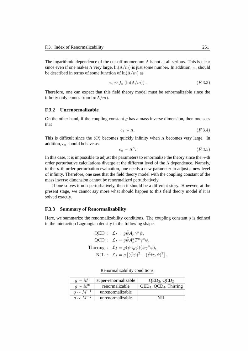
F.3. Index of Renormalizability 251
The logarithmic dependence of the cut-off momentumΛ is not at all serious. This is clearsince even if one makesΛ very large,ln(Λ/m) is just some number. In addition,cn shouldbe described in terms of some function ofln(Λ/m) as
cn ∼ fn (ln(Λ/m)) . (F.3.3)
Therefore, one can expect that this field theory model must be renormalizable since theinfinity only comes fromln(Λ/m).
F.3.2 Unrenormalizable
On the other hand, if the coupling constantg has a mass inverse dimension, then one seesthat
c1 ∼ Λ. (F.3.4)
This is difficult since the〈O〉 becomes quickly infinity whenΛ becomes very large. Inaddition,cn should behave as
cn ∼ Λn. (F.3.5)
In this case, it is impossible to adjust the parameters to renormalize the theory since then-thorder perturbative calculations diverge at the different level of theΛ dependence. Namely,to then-th order perturbation evaluation, one needs a new parameter to adjust a new levelof infinity. Therefore, one sees that the field theory model with the coupling constant of themass inverse dimension cannot be renormalized perturbatively.
If one solves it non-perturbatively, then it should be a different story. However, at thepresent stage, we cannot say more what should happen to this field theory model if it issolved exactly.
F.3.3 Summary of Renormalizability
Here, we summarize the renormalizability conditions. The coupling constantg is definedin the interaction Lagrangian density in the following shape.
QED : LI = gψAµγµψ,
QCD : LI = gψAaµT aγµψ,
Thirring : LI = g(ψγµψ)(ψγµψ),
NJL : LI = g[(ψψ)2 + (ψiγ5ψ)2
].
Renormalizability conditions
g ∼ M1 super-renormalizable QED2, QCD2
g ∼ M0 renormalizable QED4, QCD4, Thirringg ∼ M−1 unrenormalizableg ∼ M−2 unrenormalizable NJL

252 Appendix F. Regularizations and Renormalizations
QED2: Quantum electrodynamics in two dimensions D.
QCD2: Quantum chromodynamics in two dimensions D.
QED4: Quantum electrodynamics in four dimensions D.
QCD4: Quantum chromodynamics in four dimensions D.
Thirring: current- current interaction model in two dimensions D.
NJL: current- current interaction model in four dimensions D.
F.4 Infinity in Physics
In physics, there appear many kinds of infinities. Mathematically, infinity is simply denotedas∞. For example, when one has to take the thermodynamic limit, one says that the boxlengthL must be set to infinityL → ∞. However, in physics, the above equation doesnot make sense since there is no infinity in reality. In other words, if one calculates somequantity in atomic system and has to take the thermodynamic limit, thenL = 6.4 × 10⁶
m (the earth radius) is of course infinity since the atomic scale is of the order10−6 cm, atmost.
In this respect, the physical meaning ofL → ∞ is that the box lengthL must bemuch larger than any of the relevant scales in the system of the model. If one has to takean infinity in the mathematical sense, then it indicates that the model one considers is toomuch simplified and should be improved to introduce some relevant scale such that the newscale can play some role in the model.
Also, when one evaluates the momentum integral in the perturbation theory, then theintegral ranges from−Λ to Λ whereΛ is set to infinity. However, the infinity of this cutoffmomentumΛ means again that it should be much larger than any of the relevant massscalem
Λ À m.
For example, if the value ofΛ isΛ ∼ 108 m
then it is physically sufficiently larger thanm. The important point is that one should builda scheme in which physical observables should not depend on the choice of theΛ value ifit is sufficiently larger than any of the mass scales.
In this respect, the logarithmic divergenceln( Λm) is just a number for the infinity of the
cutoff momentumΛ. For example, the value ofΛ ∼ 108 m gives
ln(
Λm
)' ln 108 ' 18
which is not at all a large value. This indicates that one should not worry about the loga-rithmic divergenceln( Λ
m) when one renormalizes the infinity of the self-energy diagramsas discussed in Appendix I.
Appendix G
Path Integral Formulation
The path integral in quantum mechanics can be obtained by rewriting the quantum mechan-ical amplitudeK(x, x′ : t) into many dimensional integrations over discretized coordinatesxn. We discuss some examples which can be related to physical observables. However, thepath integral expression cannot be connected to the dynamics of classical mechanics, eventhough, superficially, there is some similarity between them. Then, we show Feynman’s for-mulation of the path integral in quantum electrodynamics (QED), which is based on manydimensional integrations over the parametersqk,λ appearing in the vector potential. Thisshould be indeed connected to the second quantization in field theory models. However,the field theory path integral formulation in most of the textbooks is normally defined interms of many dimensional integrations over fields. In this case, the path integral does notcorrespond to the field quantization. Here, we clarify what should be the problems of thepath integral formulation over the field variables and why the integrations over fields do notcorrespond to the field quantization.
G.1 Path Integral in Quantum Mechanics
The path integral formulation in one dimensional quantum mechanics starts from the am-plitudeK(x, x′ : t) which is defined by
K(x, x′ : t) = 〈x′|e−iHt|x〉, (G.1.1)
where the system is specified by the HamiltonianH. In the field theory textbooks, oneoften finds the expression of the amplitudeK(x, x′ : t) in terms of the transition betweenthe state|x, t〉 and|x′, t′〉 as
〈x′, t′|x, t〉 −→ 〈x′|e−iH(t′−t)|x〉. (G.1.2)
However, the state|x, t〉 is not an eigenstate of the Hamiltonian and therefore, one cannotprove the rightarrow of eq.(G.1.2). Instead, we should rewrite the amplitudeK(x, x′ : t) so
253

254 Appendix G. Path Integral Formulation
as to understand its physical meaning
K(x, x′ : t) = 〈x′|e−iHt|x〉 =∑
n
ψn(x′)ψ†n(x)e−iEnt, (G.1.3)
whereψn(x) andEn should be the eigenstate and the eigenvalue of the HamiltonianH. Wenote that eq.(G.1.3) is not yet directly related to physical observables.
G.1.1 Path Integral Expression
We start from the amplitudeK(x′, x : t)
K(x′, x : t) = 〈x′|e−iHt|x〉,where the Hamiltonian in one dimension is given as
H =p2
2m+ U(x) = − 1
2m
∂2
∂x2+ U(x). (G.1.4)
Here, a particle with its massm is bound in the potentialU(x). Now, one can makenpartitions oft andx′ − x, and therefore we label the discretized coordinatex as
x = x0, x1, x2, . . . , x′ = xn. (G.1.5)
In this case, we assume that eachxi andp should satisfy the following completeness rela-tions
∞∫
−∞dxi |xi〉〈xi| = 1, 〈xi|p〉 =
1√2π
eipxi ,
∞∫
−∞dp|p〉〈p| = 1 (i = 1, . . . , n), (G.1.6)
Therefore,K(x′, x : t) becomesK(x′, x : t)
=
∞∫
−∞dx1 · · ·
∞∫
−∞dxn−1 〈x′|e−iH∆t|xn−1〉〈xn−1|e−iH∆t|xn−2〉 · · · 〈x1|e−iH∆t|x〉, (G.1.7)
where∆t is defined as∆t = tn . Further, one can calculate the matrix elements, for exam-
ple, as
〈x1|e−iH∆t|x〉 = 〈x1| exp[−i
(−∆t
2m
∂2
∂x2+ U(x)∆t
)]|x〉
' exp(−iU(x)∆t)〈x1| exp(
i∆t
2m
∂2
∂x2
)|x〉+ O((∆t)2). (G.1.8)
In addition, 〈x1|ei ∆t2m
∂2
∂x2 |x〉 can be evaluated by inserting a complete set of momentumstates
〈x1| exp(
i∆t
2m
∂2
∂x2
)|x〉
G.1. Path Integral in Quantum Mechanics 255
=
∞∫
−∞
dp
2πe−i p2
2m∆t e−ip(x−x1) =
√m
2iπ∆te−i
m(x−x1)2
2∆t . (G.1.9)
Therefore, one finds now the path integral expression forK(x′, x : t)
K(x′, x : t) = limn→∞
( m
2iπ∆t
)n2 ×
∞∫
−∞dx1 · · ·
∞∫
−∞dxn−1 exp
i
n∑
k=1
(m(xk − xk−1)2
2∆t− U(xk)∆t
), (G.1.10a)
wherex0 = x andxn = x′, respectively. Since the classical actionS is given as
S =
t∫
0
dt
(12
mx2 − U(x))
= limn→∞
n∑
k=1
∆t
m
2
(xk − xk−1
∆t
)2
− U(xk)
(G.1.11)
the amplitude can be symbolically written as
K(x′, x : t) = N∫
[Dx] exp
i
t∫
0
(12
mx2 − U(x))
dt
, (G.1.10b)
whereN ∫[Dx] is defined as
N∫
[Dx] ≡ limn→∞
( m
2iπ∆t
)n2
∞∫
−∞dx1 · · ·
∞∫
−∞dxn−1.
This is indeed amazing in that the quantum mechanical amplitude is connected to the La-grangian of the classical mechanics for a particle with its massm in the same potentialU(x). Since the procedure of obtaining eq.(G.1.10) is just to rewrite the amplitude by in-serting the complete set of the|xn〉 states, there is no mathematical problem involved inevaluating eq.(G.1.10).
G.1.2 Physical Mmeaning of Path Integral
However, the physical meaning of the procedure is not at all easy to understand.It is clear that eq.(G.1.10a) is well defined and there is no problem since it simply
involves mathematics. However, there is a big jump from eq.(G.1.10a) to eq.(G.1.10b), eventhough it looks straightforward. Eq.(G.1.10b) indicates that the first term of eq.(G.1.10b)in the curly bracket is the kinetic energy of the particle in classical mechanics. In thiscase, however,xk andxk−1 cannot be varied independently as one sees it from classicalmechanics since it is related to the time derivative. On the other hand, they must be variedindependently in the original version of eq.(G.1.10a) since it has nothing to do with the

256 Appendix G. Path Integral Formulation
time derivative in the process of the evaluation. This is clear since, in quantum mechanics,time and coordinate are independent from each other. Therefore, it is difficult to interpretthe first term of eq.(G.1.10a) as the kinetic energy term in classical mechanics. Secondly,the procedure of rewriting the amplitude is closely connected to the fact that the kineticenergy of the Hamiltonian is quadratic inp, that is, it is described asp
2
2m . In this respect, thefundamental ingredients of the path integral formulation must lie in eq.(G.1.9) which relatesthe momentum operatorp2 to the time derivative of the coordinatex under the conditionthat xk andxk−1 are sufficiently close to each other. In this sense, if the kinetic energyoperator were linear inp like the Dirac equation, then there is no chance to rewrite theamplitude since the Gaussian integral is crucial in evaluating the integral.
Therefore, it should be difficult to claim that eq.(G.1.10a) can correspond to the dy-namics of classical mechanics, even though, superficially, there is some similarity be-tween them. In other words, it is hard to prove that the quantum mechanical expressionof K(x′, x : t) is related to any dynamics of classical mechanics. One may say thatK(x′, x : t) happens to have a similar shape to classical Lagrangian, mathematically, but,physically it has nothing to do with the dynamics of classical mechanics.
No summation of Classical Path
In some of the path integral textbooks, one finds the interpretation that the quantum mechan-ical dynamics can be obtained by summing up all possible paths in the classical mechanicaltrajectories. However, if one starts from eq.(G.1.10b) and tries to sum up all the possiblepaths, then one has to find the functional dependence of the coordinates on time and shouldintegrate over all the possible coordinate configurations as the function of time. This shouldbe quite different from the expression of eq.(G.1.10a). If one wishes to sum up all the pos-sible paths in eq.(G.1.10b), then one may have to first consider the following expression ofthe coordinatex as the function of time
x = xcl(t′) +∞∑
n=1
yn sin(
2πn
t
)t′,
wherexcl(t′) denotes the classical coordinate that satisfies the Newton equation of motionwith the initial conditions ofxcl(0) = x andxcl(t) = x′. The amplitudeyn is the expan-sion coefficient. Therefore, the integrations over all the paths should mean that one shouldintegrate over
∞∏
n=1
∞∫
−∞dyn
and, in this case, one can easily check that the calculated result of the integration over all thepaths cannot reproduce the proper quantum mechanical result for the harmonic oscillatorcase. This simply means that the integration overdx1 · · · dxn−1 in eq.(G.1.10a) and theintegration over classical paths are completely different from each other, which is a naturalresult. This fact is certainly known to some careful physicists, but most of the path integral
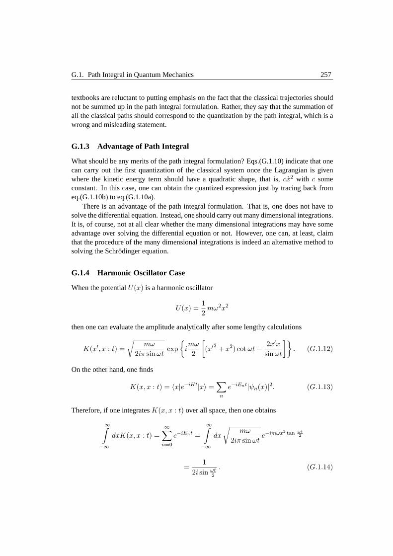
G.1. Path Integral in Quantum Mechanics 257
textbooks are reluctant to putting emphasis on the fact that the classical trajectories shouldnot be summed up in the path integral formulation. Rather, they say that the summation ofall the classical paths should correspond to the quantization by the path integral, which is awrong and misleading statement.
G.1.3 Advantage of Path Integral
What should be any merits of the path integral formulation? Eqs.(G.1.10) indicate that onecan carry out the first quantization of the classical system once the Lagrangian is givenwhere the kinetic energy term should have a quadratic shape, that is,cx2 with c someconstant. In this case, one can obtain the quantized expression just by tracing back fromeq.(G.1.10b) to eq.(G.1.10a).
There is an advantage of the path integral formulation. That is, one does not have tosolve the differential equation. Instead, one should carry out many dimensional integrations.It is, of course, not at all clear whether the many dimensional integrations may have someadvantage over solving the differential equation or not. However, one can, at least, claimthat the procedure of the many dimensional integrations is indeed an alternative method tosolving the Schrodinger equation.
G.1.4 Harmonic Oscillator Case
When the potentialU(x) is a harmonic oscillator
U(x) =12
mω2x2
then one can evaluate the amplitude analytically after some lengthy calculations
K(x′, x : t) =√
mω
2iπ sinωtexp
imω
2
[(x′2 + x2) cot ωt− 2x′x
sinωt
]. (G.1.12)
On the other hand, one finds
K(x, x : t) = 〈x|e−iHt|x〉 =∑
n
e−iEnt|ψn(x)|2. (G.1.13)
Therefore, if one integratesK(x, x : t) over all space, then one obtains
∞∫
−∞dxK(x, x : t) =
∞∑
n=0
e−iEnt =
∞∫
−∞dx
√mω
2iπ sinωte−imωx2 tan ωt
2
=1
2i sin ωt2
. (G.1.14)
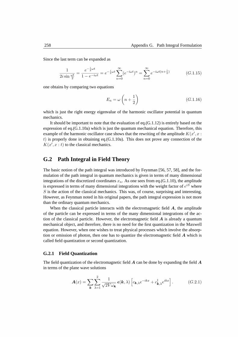
258 Appendix G. Path Integral Formulation
Since the last term can be expanded as
12i sin ωt
2
=e−
i2ωt
1− e−iωt= e−
i2ωt
∞∑
n=0
(e−iωt)n =∞∑
n=0
e−iωt(n+ 12) (G.1.15)
one obtains by comparing two equations
En = ω
(n +
12
)(G.1.16)
which is just the right energy eigenvalue of the harmonic oscillator potential in quantummechanics.
It should be important to note that the evaluation of eq.(G.1.12) is entirely based on theexpression of eq.(G.1.10a) which is just the quantum mechanical equation. Therefore, thisexample of the harmonic oscillator case shows that the rewriting of the amplitudeK(x′, x :t) is properly done in obtaining eq.(G.1.10a). This does not prove any connection of theK(x′, x : t) to the classical mechanics.
G.2 Path Integral in Field Theory
The basic notion of the path integral was introduced by Feynman [56, 57, 58], and the for-mulation of the path integral in quantum mechanics is given in terms of many dimensionalintegrations of the discretized coordinatesxn. As one sees from eq.(G.1.10), the amplitudeis expressed in terms of many dimensional integrations with the weight factor ofeiS whereS is the action of the classical mechanics. This was, of course, surprising and interesting.However, as Feynman noted in his original papers, the path integral expression is not morethan the ordinary quantum mechanics.
When the classical particle interacts with the electromagnetic fieldA, the amplitudeof the particle can be expressed in terms of the many dimensional integrations of the ac-tion of the classical particle. However, the electromagnetic fieldA is already a quantummechanical object, and therefore, there is no need for the first quantization in the Maxwellequation. However, when one wishes to treat physical processes which involve the absorp-tion or emission of photon, then one has to quantize the electromagnetic fieldA which iscalled field quantization or second quantization.
G.2.1 Field Quantization
The field quantization of the electromagnetic fieldA can be done by expanding the fieldAin terms of the plane wave solutions
A(x) =∑
k
2∑
λ=1
1√2V ωk
ε(k, λ)[ck,λe−ikx + c†k,λeikx
]. (G.2.1)
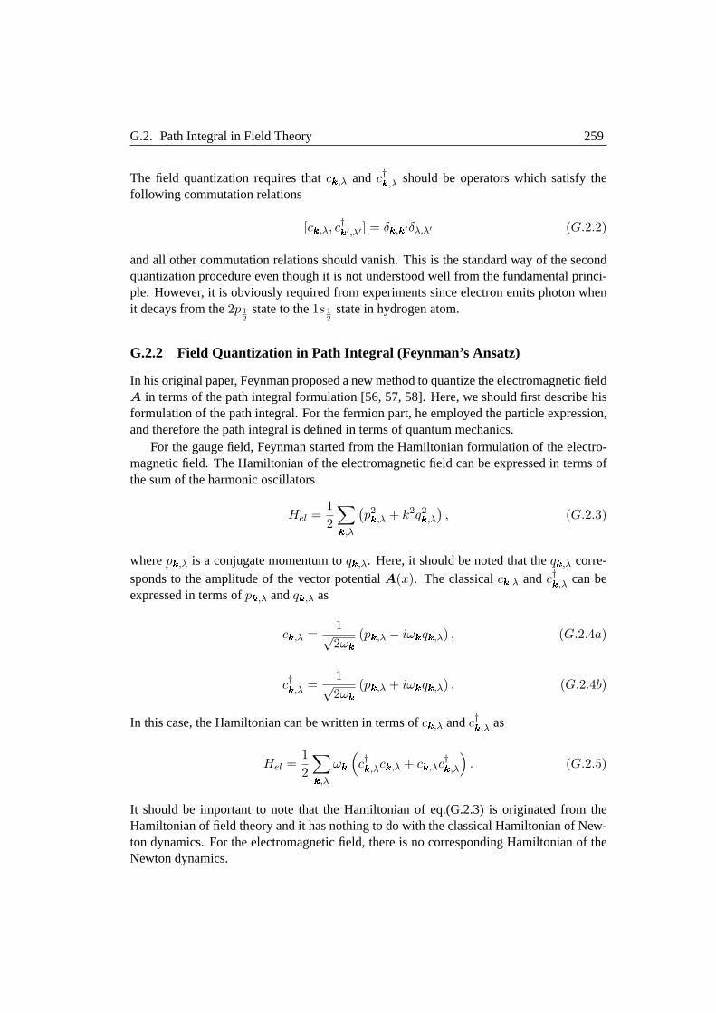
G.2. Path Integral in Field Theory 259
The field quantization requires thatck,λ and c†k,λ should be operators which satisfy thefollowing commutation relations
[ck,λ, c†k′,λ′ ] = δk,k′δλ,λ′ (G.2.2)
and all other commutation relations should vanish. This is the standard way of the secondquantization procedure even though it is not understood well from the fundamental princi-ple. However, it is obviously required from experiments since electron emits photon whenit decays from the2p 1
2state to the1s 1
2state in hydrogen atom.
G.2.2 Field Quantization in Path Integral (Feynman’s Ansatz)
In his original paper, Feynman proposed a new method to quantize the electromagnetic fieldA in terms of the path integral formulation [56, 57, 58]. Here, we should first describe hisformulation of the path integral. For the fermion part, he employed the particle expression,and therefore the path integral is defined in terms of quantum mechanics.
For the gauge field, Feynman started from the Hamiltonian formulation of the electro-magnetic field. The Hamiltonian of the electromagnetic field can be expressed in terms ofthe sum of the harmonic oscillators
Hel =12
∑
k,λ
(p2k,λ + k2q2
k,λ
), (G.2.3)
wherepk,λ is a conjugate momentum toqk,λ. Here, it should be noted that theqk,λ corre-sponds to the amplitude of the vector potentialA(x). The classicalck,λ andc†k,λ can beexpressed in terms ofpk,λ andqk,λ as
ck,λ =1√2ωk
(pk,λ − iωkqk,λ) , (G.2.4a)
c†k,λ =1√2ωk
(pk,λ + iωkqk,λ) . (G.2.4b)
In this case, the Hamiltonian can be written in terms ofck,λ andc†k,λ as
Hel =12
∑
k,λ
ωk
(c†k,λck,λ + ck,λc†k,λ
). (G.2.5)
It should be important to note that the Hamiltonian of eq.(G.2.3) is originated from theHamiltonian of field theory and it has nothing to do with the classical Hamiltonian of New-ton dynamics. For the electromagnetic field, there is no corresponding Hamiltonian of theNewton dynamics.

260 Appendix G. Path Integral Formulation
Feynman’s Ansatz
Feynman proposed a unique way of carrying out the field quantization [56, 57, 58]. Sincethe Hamiltonian of the electromagnetic field can be written as the sum of the harmonicoscillators, he presented the path integral formulation for the electromagnetic field
K(qk,λ, q′k,λ, t) ≡ N∫
[Dqk,λ] exp
i
2
t∫
0
∑
k,λ
(q2k,λ − k2q2
k,λ
)dt
(G.2.6)
which should correspond to the quantization of the variablesqk,λ, and this corresponds tothe quantization of theck,λ andc†k,λ. Thus, it is the second quantization of the electromag-netic field.
In this expression, there is an important assumption for the coordinatesqk,λ which arethe parameters appearing in the vector potential. That is, the states|qk,λ〉 should make acomplete set. Only under this assumption, one can derive the quantization of the harmonicoscillators. Since this is the parameter space, it may not be easy to prove the completenessof the states|qk,λ〉. Nevertheless, Feynman made use of the path integral expression toobtain the Feynman rules in the perturbation theory for QED. It may also be important tonote that the path integral in Feynman’s method has nothing to do with the integration ofthe configuration space. It is clear that one should not integrate out over the configurationspace in the path integral since the field quantization should be done for the parametersck,λ
andc†k,λ.
G.2.3 Electrons Interacting through Gauge Fields
When one treats the system in which electrons are interacting through electromagneticfields, one can write the whole system in terms of the path integral formulation. In thiscase, however, we treat electrons in the non-relativistic quantum mechanics. The electro-magnetic fields are treated just in the same way as the previous section.
K(qk,λ, q′k,λ, r, r′, t)
≡N∫
[Dr][Dqk,λ] exp
i
t∫
0
1
2mr2−gr ·A(r)+
12
∑
k,λ
(q2k,λ−k2q2
k,λ
) dt
, (G.2.7)
where the vector potentialA is given in eq.(G.2.1)
A(x) =∑
k
2∑
λ=1
ε(k, λ)√V ωk
[qk,λ cos(k · r) + ωkqk,λ sin(k · r)
](G.2.8)
which is now rewritten in terms of the variablesqk,λ.It should be noted that the path integral formulation works only for the electromagnetic
field since its field Hamiltonian can be described by the sum of the harmonic oscillators.
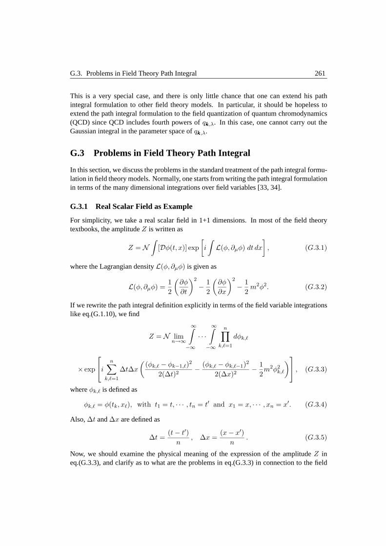
G.3. Problems in Field Theory Path Integral 261
This is a very special case, and there is only little chance that one can extend his pathintegral formulation to other field theory models. In particular, it should be hopeless toextend the path integral formulation to the field quantization of quantum chromodynamics(QCD) since QCD includes fourth powers ofqk,λ. In this case, one cannot carry out theGaussian integral in the parameter space ofqk,λ.
G.3 Problems in Field Theory Path Integral
In this section, we discuss the problems in the standard treatment of the path integral formu-lation in field theory models. Normally, one starts from writing the path integral formulationin terms of the many dimensional integrations over field variables [33, 34].
G.3.1 Real Scalar Field as Example
For simplicity, we take a real scalar field in 1+1 dimensions. In most of the field theorytextbooks, the amplitudeZ is written as
Z = N∫
[Dφ(t, x)] exp[i
∫L(φ, ∂µφ) dt dx
], (G.3.1)
where the Lagrangian densityL(φ, ∂µφ) is given as
L(φ, ∂µφ) =12
(∂φ
∂t
)2
− 12
(∂φ
∂x
)2
− 12
m2φ2. (G.3.2)
If we rewrite the path integral definition explicitly in terms of the field variable integrationslike eq.(G.1.10), we find
Z = N limn→∞
∞∫
−∞· · ·
∞∫
−∞
n∏
k,`=1
dφk,`
× exp
i
n∑
k,`=1
∆t∆x
((φk,` − φk−1,`)2
2(∆t)2− (φk,` − φk,`−1)2
2(∆x)2− 1
2m2φ2
k,`
) , (G.3.3)
whereφk,` is defined as
φk,` = φ(tk, x`), with t1 = t, · · · , tn = t′ and x1 = x, · · · , xn = x′. (G.3.4)
Also, ∆t and∆x are defined as
∆t =(t− t′)
n, ∆x =
(x− x′)n
. (G.3.5)
Now, we should examine the physical meaning of the expression of the amplitudeZ ineq.(G.3.3), and clarify as to what are the problems in eq.(G.3.3) in connection to the field

262 Appendix G. Path Integral Formulation
quantization. The first problem is that eq.(G.3.3) does not contain any quantity which isconnected to the initial and final states. This is clear since, in eq.(G.3.3), one should in-tegrate over fields as defined and therefore no information ofφ(t, x) andφ(t′, x′) is leftwhile, in quantum mechanics version, the amplitude is described by the quantitiesψn(x)andψ†n(x′) which are the eigenstates of the Hamiltonian. The second problem is that thecalculated result of the amplitudeZ must be only a function ofm,∆t, ∆x, that is
Z = f(m,∆t, ∆x). (G.3.6)
This shows that the formulation which is started from many dimensional integrations overthe fieldφ(t, x) has nothing to do with the second quantization. In addition,Z depends onthe artificial parameters∆t and∆x, and this clearly shows that it cannot be related to anyphysical observables.
This is in contrast with the formulation of eq.(G.2.7) where the amplitudeK is specifiedby the quantum number of the parameter spaceqk,λ which is connected to the state with aproper number of photons, and it must be a function ofm, g, qk,λ
K = f(m, g, qk,λ, q′k,λ). (G.3.7)
In addition, theK does not depend on the parameters∆t and∆x, which is a natural resultas one can see it from the quantum mechanical path integral formulation.
Finally, we note that the treatment of Feynman is based on the total QED Hamiltonianwhich is a conserved quantity. On the other hand, eq.(G.3.3) is based on the action whichis obtained by integrating the Lagrangian density over space and time. As one knows, theLagrangian density is not directly related to physical observables. Therefore, unless onecan confirm that the path integral is reduced to the quantum mechanical amplitude likeeq.(G.1.10), one cannot make use of the field theory path integral formulation. In fact,one cannot rewrite the expression of eq.(G.3.3) in terms of the field theory HamiltoniandensityH, contrary to the path integral formulation in quantum mechanics. This showsthat the amplitudeZ has nothing to do with the amplitudeK in eq.(G.2.7). In this respect,the amplitudeZ has no physical meaning, and therefore one cannot calculate any physicalquantities from the path integral formulation ofZ in field theory.
G.3.2 Lattice Field Theory
Most of the numerical calculations in the lattice field theory are based on the path integralformulation of eq.(G.3.3). Unfortunately, the path integral formulation of eq.(G.3.3) haslost its physical meaning, and therefore there is little chance that one can obtain any physicsout of numerical simulations of the lattice field theory. In this respect, it is, in a sense, notsurprising that the calculated result of Wilson’s area law [112] in QED is unphysical withincorrect dimensions as we saw in Chapter 8.
Since Wilson’s calculation is presented analytically, it may be worth writing again the

G.3. Problems in Field Theory Path Integral 263
result of the Wilson loop calculation in QED as given in Chapter 8
W ≡ N∏m
∏µ
∞∫
−∞dBmµ exp
(i∑
P
Bnµ +1
2g2
∑nµν
eifnµν
). (8.49)
In the strong coupling limit, one can evaluate eq.(8.49) analytically as
W ' (g2)−∆S/a2, (G.3.8)
where∆S should be an area encircled by the loop. This has the same behavior as that ofeq.(G.3.6) since the lattice constanta is equal toa = ∆x = ∆t, that is,
W = f(g,∆S, ∆x,∆t). (G.3.9)
This amplitudeW has the dependence of the artificial parameters∆t and ∆x. This iscompletely different from eq.(G.3.7), and therefore one sees that the calculation of eq.(8.49)has no physical meaning, contrary to Feynman’s treatment which has a right behavior as thefunction of the field parametersqk,λ.
G.3.3 Physics of Field Quantization
The quantization of fields is required from experiment. Yet, it is theoretically quite difficultto understand the basic physics of the field quantization. The fundamental step of the quan-tization is that the Hamiltonian one considers becomes an operator after the quantization.The reason why one considers the Hamiltonian is because it is a conserved quantity. In thisrespect, one cannot quantize the Hamiltonian density since it is not a conserved quantityyet. This is an important reason why one must quantize the field in terms of the creationand annihilation operatorck,λ and c†k,λ in QED. In this respect, it is clear that the field
quantization must be done in terms ofck,λ andc†k,λ with which the Hamiltonian in classicalQED can be described.
G.3.4 No Connection between Fields and Classical Mechanics
Here, we should make a comment on the discretized coordinates and fields. The discretizedspace is, of course, artificial, and there is no physics in the discretized fields and equations.In some textbooks, the field equation is derived from the picture that the field is constructedby the sum of springs in which the discretized coordinates of neighboring sites are con-nected by the spring. This picture can reproduce the field equation for a massless scalarfield by adjusting some parameters, even though one started from a non-relativistic classi-cal mechanics. However, this is obviously a wrong picture for a scalar field theory since thefield equation has nothing to do with classical mechanics. It is somewhat unfortunate that itmay have had some impact on the picture concerning lattice gauge field calculations as anexcuse to make use of the discretized classical fields. As we saw in the previous section, thepath integral formulation has nothing to do with the dynamics of classical mechanics, andit is, of course, clear that the field theory path integral is never connected to any dynamicsof the classical field theory.

264 Appendix G. Path Integral Formulation
G.4 Path Integral Function Z in Field Theory
As we saw in Section G.2, Feynman’s path integral formulation in terms of many dimen-sional integrations in parameter space is indeed a plausible method to quantize the fieldsin QED. However, people commonly use the expression of the amplitudeZ as defined ineq.(G.3.1).
G.4.1 Path Integral Function in QCD
The “new formulation” of the path integral in QCD was introduced by Faddeev and Popovwho wrote theS-matrix elements as [32]
〈out|in〉 ≡ Z = N∫
[DAaµ(x)] exp
[i
∫LQCDd4x
], (G.4.1)
where the definition of the path integral volume[DAaµ(x)] is just the same as the one ex-
plained in the previous section
∫[DAa
µ(x)] ≡ limn→∞
∞∫
−∞· · ·
∞∫
−∞
∏µ,a
n∏
(i,j,k,`)
dAaµ(xi
0, xj1, x
k2, x
`3). (G.4.2)
The Lagrangian densityLQCD for QCD is given as
LQCD = −12
Tr (GµνGµν) , (G.4.3)
whereGµν denotes the field strength in QCD as given in Chapter 6
Gµν = ∂µAν − ∂νAµ + ig[Aµ, Aν ]. (G.4.4)
However, the expression of the path integral in QCD in eq.(G.4.1) does not correspond tothe field quantization. One can also understand why the path integral formulation of QCDcannot be done, in contrast to Feynman’s integrations over the parameter space in QED.In QCD, the Hamiltonian for gluons contains the fourth power ofqa
k,λ, and therefore onecannot carry out the Gaussian integrations over the parametersqa
k,λ in QCD. As Feynmanstated repeatedly in his original papers, the path integral formulation is closely connectedto the Gaussian integration where the kinetic energy term in non-relativistic quantum me-chanics is always described in terms of the quadratic termp2
2m . This naturally leads to theconclusion that the path integral formulation cannot be properly constructed in QCD, andthis is consistent with the picture that QCD does not have a free Fock space due to its gaugenon-invariance.

G.4. Path Integral FunctionZ in Field Theory 265
G.4.2 Fock Space
In quantum field theory, one must prepare Fock space since the Hamiltonian becomes anoperator. The second quantized formulation is based on the creation and annihilation op-erators which act on the Fock space. In Feynman’s path integral formulation, he preparedstates which determine the number of photons in terms of|qk,λ〉. Therefore, he startedfrom the second quantized expression of the path integral formulation. However, Faddeevand Popov simply employed the same formula of the Lagrangian density, but integratedover the functionDAa
µ(x). This cannot specify any quantum numbers of the Fock space,and therefore the integration over the functionDAa
µ(x) does not correspond to the fieldquantization.

Appendix H
New Concept of Quantization
In this textbook, the first quantization of[xi, pj ] = iδij is employed to derive the Diracequation. Here, we present a new way of understanding the first quantization. From thelocal gauge invariance and the Maxwell equation, one can derive the Lagrangian density ofthe Dirac field without involving the first quantization. This leads to a new concept of thequantization itself.
H.1 Derivation of Lagrangian Density of Dirac Field fromGauge Invariance and Maxwell Equation
Dirac derived the Dirac equation by factorizing eq.(D.1.1) such that the field equation be-comes the first order in time derivative. Now, one can derive the Lagrangian density ofDirac field in an alternative way by employing the local gauge invariance and the Maxwellequation as the most fundamental principle [50].
H.1.1 Lagrangian Density for Maxwell Equation
We start from the Lagrangian density that reproduces the Maxwell equation
L = −gjµAµ − 14
FµνFµν , (H.1.1)
whereAµ is the gauge field, andFµν is the field strength and is given as
Fµν = ∂µAν − ∂νAµ.
jµ denotes the current density of matter field which couples to the electromagnetic field.From the Lagrange equation, one obtains
∂µFµν = gjν (H.1.2)
which is just the Maxwell equation as we also saw in Appendix E.
267
268 Appendix H. New Concept of Quantization
H.1.2 Four Component Spinor
Now, one can derive the kinetic energy term of the fermion Lagrangian density. First, oneassumes that the Dirac fermion should have four components
ψ =
ψ1
ψ2
ψ3
ψ4
.
This is based on the observation that electron has spin degree of freedom which is two. Inaddition, there must be positive and negative energy states since it is a relativistic field, andtherefore the fermion field should have 4 components.
16 Independent Components
Now, the matrix elements
ψ†Oψ
can be classified into 16 independent Lorentz invariant components as
ψψ : scalar, ψγ5ψ : pseudo− scalar, (H.1.3a)
ψγµψ : 4 component vector, ψγµγ5ψ : 4 component axial-vector, (H.1.3b)
ψσµνψ : 6 component tensor, (H.1.3c)
whereψ is defined for convenience as
ψ = ψ†γ0.
These properties are determined by mathematics.
Shape of Vector Current
From the invariance consideration, one finds that the vector currentjµ must be written as
jµ = C0ψγµψ, (H.1.4)
whereC0 is a constant. Since one can renormalize the constantC0 into the coupling con-stantg, one can set without loss of generality
C0 = 1. (H.1.5)
H.2. Shape of Lagrangian Density 269
H.2 Shape of Lagrangian Density
Now, one can make use of the local gauge invariance of the Lagrangian density, and onesees that the following shape of the Lagrangian density can keep the local gauge invariance
L = C1ψ∂µγµψ − gψγµψAµ − 14
FµνFµν , (H.2.1)
whereC1 is a constant. At this point, one requires that the Lagrangian density should beinvariant under the local gauge transformation
Aµ −→ Aµ + ∂µχ, (H.2.2a)
ψ −→ e−igχψ. (H.2.2b)
In this case, it is easy to find that the constantC1 must be
C1 = i. (H.2.3)
Here, the constanth should be included implicitly into the constantC1. The determinationof h can be done only when one compares calculated results with experiment such as thespectrum of hydrogen atom.
H.2.1 Mass Term
The Lagrangian density of eq.(H.2.1) still lacks the mass term. Since the mass term mustbe a Lorentz scalar, it should be described as
C2ψψ (H.2.4)
which is, of course, gauge invariant as well. This constantC2 should be determined againby comparing the calculated results of hydrogen atom, for example, with experiment. BydenotingC2 as(−m), one arrives at the Lagrangian density of a relativistic fermion whichcouples with the electromagnetic fieldsAµ
L = iψ∂µγµψ − gψγµψAµ −mψψ − 14
FµνFµν (H.2.5)
which is just the Lagrangian density for the Dirac field interacting with electromagneticfields.
H.2.2 First Quantization
It is important to note that, in the procedure of deriving the Lagrangian density of eq.(H.2.5),one has not made use of the quantization condition of
E → i∂
∂t, p → −i∇. (H.2.6)
Instead, the first quantization is automatically done by the gauge condition since theMaxwell equation knows the first quantization in advance. This indicates that there maybe some chance to understand the first quantization procedure in depth since this methodgives an alternative way of the quantization condition of the energy and momentum.
270 Appendix H. New Concept of Quantization
H.3 Two Component Spinor
The derivation of the Dirac equation in terms of the local gauge invariance shows that thecurrent density that can couple to the gauge fieldAµ must be rather limited. Here, wediscuss a possibility of finding field equation for the two component spinor. When the fieldhas only two components,
φ =(
φ1
φ2
)
then one can prove that one cannot make the currentjµ that couples with the gauge fieldAµ. This can be easily seen since the matrix elements
φ†Oφ
can be classified into 4 independent variables as
φ†φ : scalar, φ†σkφ : 3 component vector. (H.3.1)
Therefore, there is no chance to make four vector currents which may couple to the gaugefield Aµ. This way of making the Lagrangian density indicates that it should be difficult tofind a Lagrangian density of relativistic bosons.
H.4 Klein–Gordon Equation
In the new picture, the correspondence between (E,p) and the differential operators(i ∂
∂t ,−i∇) can be obtained as a consequence from the Dirac equation
Dirac equation=⇒ E → i∂
∂t, p → −i∇.
Therefore, it should not be considered as the fundamental principle any more. This equationcan be applied to the non-relativistic motion since the Dirac equation can be reduced to theSchrodinger equation in the non-relativistic limit. However, one cannot apply the aboverelations to the relativistic kinematics since they are not the fundamental principle any more.In this respect, the derivation of the Schrodinger equation by the replacement of the energyand momentum by eq.(H.2.6)
E =p2
2m=⇒ i
∂ψ
∂t= − 1
2m∇2ψ
can be justified, but the Klein–Gordon equation
E2 = p2 + m2 =⇒ −∂2ψ
∂t2=
(−∇2 + m2)ψ
may not be justified any more. Therefore, this picture shows that the Klein–Gordon equa-tion should not be taken as the fundamental equation for the elementary particles.

H.5. Incorrect Quantization in Polar Coordinates 271
At the present stage, there is no way to derive the Klein–Gordon equation within thenew picture. Therefore, it is most likely that there should not exist any elementary Klein–Gordon field of scalar bosons in nature, and in fact there is no elementary scalar bosonobserved up to now. However, the study of scalar field is mathematically an interestingsubject, and one may learn some new aspects in boson fields in a future study.
In nature, there exist bosons, and they are all composite objects which have integerspins. For the composite boson which is composed of fermion and anti-fermion, a Klein–Gordon type equation should be obtained from the two particle Dirac equation. However,it may not be very easy to derive the equation for the center of mass motion for the twoparticle system in the Dirac equation since it involves the relativistic kinematics. But stilltheoretically it must be a doable calculation.
H.5 Incorrect Quantization in Polar Coordinates
In the standard quantum mechanical treatment, the particle Hamiltonian in polar coordinatesin classical mechanics cannot be quantized in the canonical formalism. In order to see thissituation more explicitly, one can write a free particle Hamiltonian with its massm in polarcoordinates
H =pr
2
2m+
pθ2
2mr2+
pϕ2
2mr2 sin2 θ, (H.5.1)
wherepr, pθ, pϕ are the generalized momenta in polar coordinates in classical mechanics.If one quantizes the Hamiltonian with the canonical quantization conditions
[r, pr] = i, [θ, pθ] = i, [ϕ, pϕ] = i (H.5.2)
then one obtains
H = − 12m
(∂2
∂r2+
1r2
∂2
∂θ2+
1r2 sin2 θ
∂2
∂ϕ2
)(H.5.3)
which is not a correct Hamiltonian for a free particle in polar coordinates. The correctHamiltonian for a free particle is, of course, given as
H = − 12m
(1r2
∂
∂rr2 ∂
∂r
)− 1
2mr2
(1
sin θ
∂
∂θsin θ
∂
∂θ+
1sin2 θ
∂2
∂ϕ2
)(H.5.4)
which is obtained by transforming the Schrodinger equation in Cartesian coordinates intopolar coordinates.
Now, we can explain the reason why the quantization condition is valid for the Cartesiancoordinates, but not for the polar coordinates. In the new picture, the differential operatorsfirst appear in the Dirac equation and then the momentum is identified as the correspond-ing differential operator. Therefore, the Schrodinger equation is obtained from the Diracequation, but not from the Hamiltonian of classical mechanics in the canonical formalismby replacing the generalized momenta by the corresponding differential operators.
272 Appendix H. New Concept of Quantization
H.6 Interaction with Gravity
The chain of the fundamental equations from classical mechanics to Dirac equation is nowreversed
Dirac equation=⇒ Schrodinger equation=⇒ Newton equation.
At this point, however, one realizes that there is no way to include the gravitational forceinto the new system. This may be a serious defect of this new concept of the first quantiza-tion. However, if the gravity is included in this formalism, then it means that the quantumtheory of gravity can be constructed.

Appendix I
Renormalization in QED
This textbook treats mainly the non-perturbative aspects of quantum field theory of fermionsand therefore we have only briefly discussed the perturbation theory in QED in Chap-ter 5. In this Appendix, we present some of the basic ingredients in the renormalizationscheme in the perturbative evaluation in QED. However, we only describe the basic con-cept of the renormalization scheme since calculations in detail are found in the textbookof Bjorken-Drell [14]. The essential difference between the perturbative evaluation andthe non-perturbative treatment should be found in the Fock space which can be prepared inadvance in the perturbative treatment while one does not know the eigenstates of the Hamil-tonian in the non-perturbative calculation where one has to solve the eigenvalue equation ofeq.(3.1).
I.1 Hilbert Space of Unperturbed Hamiltonian
First, we start from the QED Lagrangian densityL which is composed of the unperturbedLagrangian densityL0 and the interaction termLI
L0 = ψ(p/−m)ψ − 14
FµνFµν , (I.1.1)
LI = −eAµψγµψ. (I.1.2)
In this case, the unperturbed HamiltonianH0 can be constructed from the Lagrangian den-sityL0 as given in eq.(5.28a) in Chapter 5. The Hilbert space of the quantized HamiltonianH0 can be well constructed since one finds the exact eigenvalues and eigenstates of eq.(3.1)for theH0. In this case, the Fock space can be specified by the box lengthL and the cutoffmomentumΛ as well as by the energies and momenta of the free fermion and free gaugefield states
(L,Λ) :
Ep =√
p2n + m2, pn =
2πn
L
ωk = |kn|, kn =2πn
L
, (I.1.3)
273

274 Appendix I. Renormalization in QED
ni = 0,±1, . . . ,±N with Λ =2πN
L,
where the maximum number of freedomN is taken to be the same between the fermionand the gauge fields. The perturbative evaluation can be made within this Hilbert space andone can calculate physical quantities in terms of theS-matrix formulation.
In the evaluation of the second order perturbation energy, there are some diagramswhich are divergent. However, the momentum integral has the cutoff due to theΛ, andtherefore, the second order energies are described as the function ofln(Λ/m). Among thedivergent diagrams, the photon self-energy contribution (vacuum polarization diagram) isspecial, and therefore we will teat it separately in Appendix J. Here, we discuss the fermionself-energy diagram and the vertex correction contribution.
I.2 Necessity of Renormalization
Before explaining the divergent contribution of the self-energy diagrams, we should un-derstand reasons why we should make a renormalization procedure [59, 103, 107]. Thefermion self-energy diagram itself is obviously unphysical since the fermion with its mo-mentump goes to the same fermion with the same momentump after emitting a photonand absorbing the same photon. This process itself cannot be observed and examined ex-perimentally. Why is it then necessary to consider the fermion self-energy diagram into therenormalization procedure?
I.2.1 Intuitive Picture of Fermion Self-energy
The answer to the above question is simple. We should consider the following situation inwhich the fermion is found in the different quantum state from the free state. For example, ifwe consider electron in hydrogen atom, then its quantum state should be very different fromthe free state. In this case, the fermion self-energy diagram gives a physical contributionwhich is observed as the Lamb shift energy. Basically, in the renormalization procedure, weconsider a counter term which can exactly cancel the divergent contribution of the secondorder self-energy diagrams in the free state of fermions. However, in atom, this cancellationdoes not have to take place in an exact fashion, and this small effect of difference gives riseto the Lamb shift energy in1s 1
2and2s 1
2states in hydrogen atom.
I.2.2 Intuitive Picture of Photon Self-energy
On the other hand, the photon self-energy is quite different in that photon can never becomea bound state. It is always found as a free state. Therefore, there is no physical process inwhich the contribution of the photon self-energy is detectable in some way or the other. Infact, there has been no physical processes which show the effect of the simple self-energydiagrams.

I.3. Fermion Self-energy 275
I.3 Fermion Self-energy
Now, the fermion self-energyΣ(p) is obtained from the corresponding Feynman diagram as
Σ(p) = −ie2
∫d4k
(2π)4γµ
1p/− k/−m
γµ 1k2
. (I.3.1)
This can be calculated to be
Σ(p) =e2
8π2ln
(Λm
)(−p/ + 4m) + finite terms. (I.3.2)
Therefore, the Lagrangian density of the free fermion part
LF = ψ(p/−m)ψ (I.3.3)
should be modified, up to one loop contributions, by the counter termδLF
δLF = ψ
[e2
8π2ln
(Λm
)(−p/ + 4m)
]ψ.
In this case, the total Lagrangian density of fermion becomes
L′F = LF + δLF = ψ [(1 + B)p/− (1 + A)m]ψ + finite terms, (I.3.4)
where
A = − e2
2π2ln
(Λm
), B = − e2
8π2ln
(Λm
). (I.3.5)
Now, one definesZ2 andδm as
Z2 ≡ 1 + B = 1− e2
8π2ln
(Λm
), (I.3.6a)
δm ≡ 3e2m
8π2ln
(Λm
). (I.3.6b)
Here, one can introduce the wave function renormalization and the bare massm0
ψb ≡√
Z2ψ =√
1 + Bψ, (I.3.7a)
m0 ≡ Z−12 m(1 + A)
= m
(1 +
e2
8π2ln
(Λm
))(1− e2
2π2ln
(Λm
))' m− δm, (I.3.7b)
where one should always keep up to order ofe2. In this case, one can rewriteL′F as
L′F = ψb(p/−m0)ψb + finite terms (I.3.8)
which has just the same shape as the original one, and thus it is renormalizable.

276 Appendix I. Renormalization in QED
I.4 Vertex Corrections
The vertex corrections can be evaluated as
Λµ(p′, p) = −ie2
∫d4k
(2π)4γν 1
p/′ − k/−mγµ 1
p/− k/−mγν
1k2
=e2
8π2ln
(Λm
)γµ + finite terms. (I.4.1)
Therefore, the counter term of the interaction Lagrangian densityδLI becomes
δLI =e3
8π2ln
(Λm
)Aµψγµψ.
In this case, the total interaction Lagrangian density can be written as
L′I = −eAµψγµψ + δLI = −Z1eAµψγµψ + finite terms, (I.4.2)
whereZ1 is defined as
Z1 ≡ 1− e2
8π2ln
(Λm
). (I.4.3)
From eqs.(I.3.6) and (I.4.3), one finds
Z1 = Z2. (I.4.4)
This can be also understood from the following identity
∂
∂pµ
(1
p/−m
)= − 1
p/−mγµ 1
p/−m. (I.4.5)
Therefore, one finds
Λµ(p, p) = −∂Σ(p)∂pµ
(I.4.6)
which leads to eq.(I.4.4). The interaction Lagrangian density can be rewritten in terms ofthe bare quantities
ψb ≡√
Z2ψ (I.4.7)
as
L′I = −Z1eAµψγµψ = −Z1e
1Z2
Aµψbγµψb = −ebAµψbγµψb + finite terms, (I.4.8)
where the bare chargeeb turns out to be
eb = e. (I.4.9)
Therefore, all the infinite quantities are renormalized into the physical constants as wellas the wave function. It should be important that the chargee is not affected from therenormalization.

I.5. New Aspects of Renormalization in QED 277
I.5 New Aspects of Renormalization in QED
The renormalization scheme in QED is best studied and most reliable. Nevertheless thereis one important modification in the renormalization procedure, and it is connected to thetreatment of the photon self-energy diagram. It turns out that the photon self-energy con-tribution should not be considered for the renormalization procedure since the contributionitself is unphysical. The detailed discussion of the photon self-energy in QED is treated inAppendix J. This gives rise to some important consequences. The most important of all isthat the charge is not affected by the renormalization procedure. This means that there is norenormalization group equation. Here, we should first like to discuss the old version of therenormalization group equation in QED and then compare the new simple picture whichhas no renormalization group equation since the charge has no renormalization effect.
I.5.1 Renormalization Group Equation in QED
(1) Old Version
For the renormalization group equation, people start from the following equation for therenormalized coupling constanteb
eb = eZ1λε2
1Z2
√Z3
= eλε2
(1 +
e2
12π2ε
), (I.5.1)
whereλ is a parameter which is introduced in the dimensional regularization andε is aninfinitesimally small number. Here,Z3 is defined as
Z3 = 1− e2
6π2ε
which comes from the wave function renormalization of the photon self-energy contribu-tion. Even though eq.(I.5.1) is obtained from renormalizing all of the self-energy diagramstogether with the vertex corrections, this renormalization of the coupling constanteb is basi-cally originated from the photon self-energy contribution since the renormalization constantZ1 of the vertex correction and the fermion wave function renormalizationZ2 cancel witheach other because ofZ1 = Z2. Since theeb should not depend on the scaleλ, one canobtain the renormalization group equation
λ∂e
∂λ= −e
2
(1− e2
4π2ε
)(ε +
e2
12π2
)= − ε
2e +
112π2
e3 + O(e5). (I.5.2)
When one makesε → 0, then one finds
λ∂e
∂λ=
112π2
e3 (I.5.3)

278 Appendix I. Renormalization in QED
which is the renormalization group equation for QED. This equation can be easily solvedfor e. The expression for the running coupling constantα(λ) ≡ e2
4π is given as
α(λ) =α(λ0)
1− 2α(λ0)3π ln( λ
λ0), (I.5.4)
whereλ0 denotes the renormalization point for the coupling constant. This is the standardprocedure to obtain the behavior of the coupling constant as the function of theλ.
However, theλ does not appear in the Hilbert space of the unperturbed HamiltonianH0 and this means that one cannot interpret the result of eq.(I.5.4) in terms of the physicalobservables which should be found in the unperturbed Fock space. Thereforeα(λ) doesnot have any physical meaning at all.
(2) New Version
The fact that the photon self-energy contribution should not be considered for the renormal-ization procedure has many important consequences. The most important is that the chargeis not influenced from the renormalization as one can see it from eq.(I.4.9) and, therefore,there is no renormalization group equation in QED. The idea of the renormalization groupequation itself is gone.
I.6 Renormalization in QCD
When one wishes to carry out the perturbation calculation, then one should first constructthe free Fock space since all of the perturbative evaluations aim at describing physicalobservables in terms of the free state physical quantities. However, QCD has intrinsicdifficulties to construct the free Fock space.
I.6.1 Fock Space of Free Fields
The normal perturbation theory always starts from the free field Hilbert space which is madefrom the unperturbed HamiltonianH0. This free field Fock space must be constructed fromthe physical states as long as one stays in the perturbation theory. However, in QCD, thereis no free quark state in nature due to the gauge non-invariance of the quark color charge.In fact, if one defines the unperturbed Lagrangian densityL0 for QCD as
L0 = ψ(p/−m)ψ − 14
(∂µAaν − ∂νA
aµ)(∂µAν,a − ∂νAµ,a)
then, one finds that it is not invariant under the local gauge transformation of eqs.(6.7) and(6.8). Even for the free fermion part, it transforms under eq.(6.7) as
ψ′(p/−m)ψ′ = ψ(p/−m)ψ − g(∂µχa)jaµ = ψ(p/−m)ψ − g∂µ(χaja
µ) + g(∂µjaµ)χa
which is not invariant since the vector current is not conserved (∂µjaµ 6= 0) for QCD, con-
trary to QED.

I.7. Renormalization of Massive Vector Fields 279
I.6.2 Renormalization Group Equation in QCD
Therefore, one cannot find any perturbation scheme in QCD, and there is no renormaliza-tion. In this respect, the gluon coupling constant is not affected from the renormalization.This is always true even if one could define some type of the perturbation theory by hand.Therefore, there is no renormalization group equation for QCD, and thus the concept of theasymptotic freedom has lost its physical meaning.
I.6.3 Serious Problems in QCD
However, OCD has much more serious problems than the lack of the QCD renormalizationgroup equation. As we stress above, we cannot carry out the perturbative calculations sincethere is no free Fock state in QCD. This means that one cannot describe any physical quan-tities in terms of the free Fock state terminology since the free states of quarks and gluonsdo not exist as the physical states. In this respect, the evaluation of QCD cannot be basedon the perturbation scheme and therefore one has to invent a new scheme to solve QCD.This is a very important problem which should be solved in some way or the other in future[35].
I.7 Renormalization of Massive Vector Fields
Since the self-energy of boson fields should not be considered for the renormalization pro-cedure, there are many important consequences concerning the renormalizability of themodel field theory. Here, we should briefly discuss the renormalization procedure of themassive vector fields which interact with fermion fields. The simplest Lagrangian densityfor two flavor leptons which couple to the SU(2) vector fieldsW a
µ can be written as
L = Ψ(i∂µγµ + m)Ψ− gJaµWµ,a +
12
M2W aµWµ,a − 1
4Ga
µνGµν,a, (I.7.1)
whereM denotes the mass of the vector boson. The fermion wave functionΨ has twocomponents.
Ψ =(
ψ1
ψ2
). (I.7.2)
Correspondingly, the mass matrix can be written as
m =(
m1 00 m2
). (I.7.3)
The fermion currentJaµ and the field strengthGa
µν are defined as
Jaµ = ΨγµτaΨ, Ga
µν = ∂µW aν − ∂νW
aµ . (I.7.4)
This Lagrangian density is almost the same as the standard model Lagrangian density apartfrom the Higgs fields, as far as the basic structure of the field theory is concerned.

280 Appendix I. Renormalization in QED
I.7.1 Renormalizability
Now, one can easily examine the renormalizability of the model field theory, and one canprove that the fermion self-energy has the logarithmic divergence which is just the sameas the QED case. Also, the vertex correction in this model field theory has the logarithmicdivergence and is the same as the QED case as long as the renormalizability is concerned.Since one should not consider the self-energy of the massive vector fields, one can safelyrenormalize the divergent contributions of the fermion self-energy as well as the vertexcorrection.
In this sense, this is just similar to checking the renormalizability of thefinal Lagrangiandensity of the standard model, and it is indeed renormalizable. This is quite important sincethe final Lagrangian density of the Weinberg-Salam model is quite successful for describingthe experiment even though the Higgs mechanism itself is not a correct procedure in termsof the symmetry breaking physics as discussed in Chapter 4.

Appendix J
Photon Self-energy Contribution inQED
In the renormalization procedure of QED, one considers the vacuum polarization which isthe contribution of the self-energy diagram of photon
Πµν(k) = ie2
∫d4p
(2π)4Tr
[γµ 1
p/−mγν 1
p/− k/−m
]. (J.0.1)
This integral obviously gives rise to the quadratic divergence (Λ2 term). However, when oneconsiders the counter term of the Lagrangian density which should cancel this quadratic di-vergence term, then the counter Lagrangian density violates the gauge invariance since itshould correspond to the mass term in the gauge field Lagrangian density. Therefore, onehas to normally erase it by hand, and in the cutoff procedure of the renormalization scheme,one subtracts the quadratic divergence term such that one can keep the gauge invariance ofthe Lagrangian density. Here, we should notice that the largest part of the vacuum polariza-tion contributions is discarded, and this indicates that there must be something which is notfully understandable in the renormalization procedure. Physically, it should be acceptableto throw away theΛ2 term since this infinite term should not be connected to any physicalobservables. Nevertheless we should think it over why the unphysical infinity appears inthe self-energy diagram of photon.
On the other hand, the quadratic divergence term disappears in the treatment of the di-mensional regularization scheme. Here, we clarify why the quadratic divergence term doesnot appear in the dimensional regularization treatment. That is, the treatment of the dimen-sional regularization employs the mathematical formula which is not valid for the evaluationof the momentum integral. Therefore, the fact that there is no quadratic divergence termin the dimensional regularization is simply because one makes a mistake by applying theinvalid mathematical formula to the momentum integral. This is somewhat surprising, butnow one sees that the quadratic divergence is still there in the dimensional regularization,and this strongly indicates that we should reexamine the effect of the photon self-energydiagram itself.
281

282 Appendix J. Photon Self-energy Contribution in QED
J.1 Momentum Integral with Cutoff Λ
This procedure of the photon self-energy is well explained in the textbook of Bjorken andDrell, and therefore we describe here the simplest way of calculating the momentum inte-gral. The type of integral one has to calculate can be summarized as
∫d4p
1(p2 − s + iε)n
= iπ2
Λ2∫
0
w dw1
(w − s + iε)n, with w = p2, (J.1.1)
wherei appears because the integral is rotated into the Euclidean space and this correspondsto D = 4 in the dimensional regularization as we will see it below.
J.1.1 Photon Self-energy Contribution
The photon self-energy contributionΠµν(k) in eq.(J.0.1) can be easily evaluated as
Πµν(k) =4ie2
(2π)4
1∫
0
dz
∫d4p
[2pµpν − gµνp
2 + sgµν − 2z(1− z)(kµkν − k2gµν)(p2 − s + iε)2
]
=α
2π
1∫
0
dz
Λ2∫
0
dw
[w(w − 2s)gµν + 4z(1− z)w(kµkν − k2gµν)
(w − s + iε)2
], (J.1.2)
wheres is defined ass = m2 − z(1− z)k2. This can be calculated to be
Πµν(k) = Π(1)µν (k) + Π(2)
µν (k),
where
Π(1)µν (k) =
α
2π
(Λ2 + m2 − k2
6
)gµν (J.1.3a)
Π(2)µν (k)=
α
3π(kµkν−k2gµν)
ln
(Λ2
m2e
)−6
1∫
0
dzz(1−z) ln(
1− k2
m2z(1−z)
). (J.1.3b)
Here, theΠ(1)µν (k) term corresponds to the quadratic divergence term and this should be
discarded since it violates the gauge invariance. TheΠ(2)µν (k) term can keep the gauge
invariance, and therefore one can renormalize it into the new Lagrangian density.
J.1.2 Finite Term in Photon Self-energy Diagram
After the renormalization, one finds a finite term which should affect the propagator changein the process involving the exchange of the transverse photonA. The propagator1
q2 should
J.2. Dimensional Regularization 283
be replaced by
1q2
=⇒ 1q2
1 +
2α
π
1∫
0
dz z(1− z) ln(
1− q2z(1− z)m2
) , (J.1.4)
whereq2 should becomeq2 ≈ −q2 for smallq2. It should be important to note that thecorrection term arising from the finite contribution of the photon self-energy should affectonly for the renormalization of the vector fieldA. Since the Coulomb propagator is notaffected by the renormalization procedure of the transverse photon (vector fieldA), oneshould not calculate its effect on the Lamb shift.
J.2 Dimensional Regularization
In the evaluation of the momentum integral, one can employ the dimensional regularization[72, 73] where the integral is replaced as
∫d4p
(2π)4−→ λ4−D
∫dDp
(2π)D, (J.2.1)
whereλ is introduced as a parameter which has a mass dimension in order to compensatethe unbalance of the momentum integral dimension. This is the integral in the Euclideanspace, butD is taken to beD = 4− ε whereε is an infinitesimally small number.
J.2.1 Photon Self-energy Diagram withD = 4− ε
In this case, the photon self-energyΠµν(k) can be calculated to be
Πµν(k) = iλ4−De2
∫dDp
(2π)DTr
[γµ
1p/−m
γν1
p/− k/−m
]
=α
3π(kµkν − gµνk
2)[2ε
+ finite term
], (J.2.2)
where the finite term is just the same as eq.(J.1.3). In eq.(J.2.2), one sees that the quadraticdivergence term (Π(1)
µν (k)) is missing. This is surprising since the quadratic divergence termis the leading order contribution in the momentum integral, and whatever one invents in theintegral, there is no way to erase it unless one makes a mistake.
J.2.2 Mathematical Formula of Integral
Indeed, in the treatment of the dimensional regularization, people employ the mathematicalformula which is invalid for the integral in eq.(J.2.2). That is, the integral formula forD = 4− ε
∫dDp
pµpν
(p2−s+iε)n= iπ
D2 (−1)n+1 Γ(n− 1
2D−1)2Γ(n)
gµν
sn− 12D−1
(for n≥3) (J.2.3)

284 Appendix J. Photon Self-energy Contribution in QED
is only valid forn ≥ 3 in eq.(J.2.3). Forn = 3, the integral should have the logarithmicdivergence, and this is nicely avoided by the replacement ofD = 4 − ε. However, then = 2 case must have the quadratic divergence and the mathematical formula of eq.(J.2.3)is meaningless. In fact, one should recover the result of the photon self-energy contributionΠµν(k) of eqs.(J.1.3) at the limit ofD = 4, apart from the(2/ε) term which correspondsto the logarithmic divergence term.
J.2.3 Reconsideration of Photon Self-energy Diagram
In mathematics, one may define the gamma function in terms of the algebraic equationswith complex variables. However, the integral in the renormalization procedure is definedonly in real space integral, and the infinity of the integral is originated from the infinitedegrees of freedom which appear in the free Fock space as discussed in Appendix I.
Therefore, one sees that the disappearance of the quadratic divergence term in the eval-uation ofΠµν(k) in the dimensional regularization is not due to the mathematical trick, but
simply due to a simple-minded mistake. In this respect, it is just accidental that theΠ(1)µν (k)
term in the dimensional regularization vanishes to zero. Indeed, one should obtain the sameexpression of theΠ(1)
µν (k) term as eq.(J.1.3a) when one makesε → 0 in the calculation ofthe dimensional regularization. This strongly suggests that we should reconsider the photonself-energy diagram itself in the renormalization procedure [45].
J.3 Propagator Correction of Photon Self-energy
In order to examine whether the inclusion of the photon self-energy contribution is neces-sary for the renormalization procedure or not, we should consider the effect of the finitecontribution from the photon self-energy diagram. As we see, there is a finite contributionof the transverse photon propagator to physical observables after the renormalization of thephoton self-energy. The best application of the propagator correction must be the magnetichyperfine splitting of the ground state (1s 1
2state) in the hydrogen atom since this interaction
is originated from the vector fieldA which gives rise to the magnetic hyperfine interactionbetween electrons and nucleus.
J.3.1 Lamb Shift Energy
In some of the textbooks [14], the correction term arising from the finite contribution of thephoton self-energy diagram is applied to the evaluation of the Lamb shift energy in hydro-gen atom. However, this is not a proper application since only the renormalization of thevector fieldA should be considered. This is closely connected to the understanding of thefield quantization itself. One sees that the second quantization of the electromagnetic fieldshould be made only for the vector fieldA, and this is required from the experimental ob-servation that photon is created from the vacuum of the electromagnetic field in the atomic
J.3. Propagator Correction of Photon Self-energy 285
transitions. Therefore, it is clear that the renormalization becomes necessary only for thevector fieldA.
Classical Picture of Polarization
This classical picture of the fermion pair creations (Uehling potential) should come fromthe misunderstanding of the structure of the vacuum state [65, 66, 110]. In the medium ofsolid state physics, the polarization can take place when there is an electric field present. Inthis case, the electric field can indeed induce the electric dipole moments in the medium,and this corresponds to the change of the charge density. However, this is a physical processwhich can happen in the real space (configuration space). On the other hand, the fermionpair creation in the vacuum in field theory is completely different in that the negative energystates are all filled in momentum space, and the time independent field ofA0 which is onlya function of coordinates cannot induce any changes on the vacuum state. Therefore, unlesssome time dependent field is present in the reaction process, the pair creation of fermionscannot take place in physical processes. Therefore, in contrast to the common belief, thereis, unfortunately, no change of the charge distribution in QED vacuum, even at the presenceof two charges, and this is basically because the Coulomb field is not time dependent.
J.3.2 Magnetic Hyperfine Interaction
The magnetic hyperfine interaction between electron and proton in hydrogen atom can bewritten with the static approximation in the classical field theory as
H ′ = −∫
je(r) ·A(r) d3r, (J.3.1)
whereje(r) denotes the current density of electron, andA(r) is the vector potential gener-ated by proton and is given as
A(r) =14π
∫Jp(r′)|r − r′| d
3r′, (J.3.2)
whereJp(r) denotes the current density of proton. The hyperfine splitting of the groundstate in the hydrogen atom can be calculated as
∆Ehfs = 〈1s 12, I : F |H ′|1s 1
2, I : F 〉, (J.3.3)
whereI andF denote the spins of proton and atomic system, respectively. This can beexplicitly calculated as
∆Ehfs = (2F (F + 1)− 3)αgp
3Mp
∞∫
0
F (1s)(r)G(1s)(r) dr, (J.3.4)

286 Appendix J. Photon Self-energy Contribution in QED
wheregp andMp denote the g-factor and the mass of proton, respectively.F (1s)(r) andG(1s)(r) are the small and large components of the radial parts of the Dirac wave functionof electron in the atom. In the nonrelativistic approximation, the integral can be expressedas ∞∫
0
F (1s)(r)G(1s)(r) dr ' (mrα)3
me, (J.3.5a)
whereme is the mass of electron andmr denotes the reduced mass defined as
mr =me
1 + meMp
. (J.3.6)
It should be noted that, in eq.(J.3.5),me appears in the denominator because it is originatedfrom the current density of electron. Therefore, the energy splitting betweenF = 1 andF = 0 atomic states in the nonrelativistic limit with a point nucleus can be calculated fromEq.(J.3.4) as
∆E(0)hfs =
8α4m3r
3meMp. (J.3.7)
J.3.3 QED Corrections for Hyperfine Splitting
There are several corrections which arise from the various QED effects such as the anoma-lous magnetic moments of electron and proton, nuclear recoil effects and relativistic effects.We write the result
∆E(QED)hfs =
4gpα4m3
r
3meMp(1 + ae)
(1 +
32
α2
)(1 + δR), (J.3.8)
whereae denotes the anomalous magnetic moment of electron. The term(1+ 32 α2) appears
because of the relativistic correction of the electron wave function∞∫
0
F (1s)(r)G(1s)(r) dr =(mrα)3
me
(1 +
32
α2 + · · ·)
. (J.3.5b)
The termδR corresponds to the recoil corrections and can be written as [16]
δR = α2
(ln 2− 5
2
)− 8α3
3πln α
(ln α− ln 4 +
281480
)+
15.4α3
π. (J.3.9)
Now the observed value of∆E(exp)hfs is found to be [30]
∆E(exp)hfs = 1420.405751767 MHz.
Also, we can calculate∆E(0)hfs and∆E
(QED)hfs numerically and their values become
∆E(0)hfs = 1418.83712 MHz, ∆E
(QED)hfs = 1420.448815 MHz.

J.3. Propagator Correction of Photon Self-energy 287
Therefore, we find the deviation from the experimental value as
∆E(exp)hfs −∆E
(QED)hfs
∆E(0)hfs
' −30 ppm. (J.3.10)
J.3.4 Finite Size Corrections for Hyperfine Splitting
In addition to the QED corrections, there is a finite size correction of proton and its effectcan be written as
∆E(FS)hfs = ∆E
(0)hfs(1 + ε), (J.3.11)
where theε term corresponds to the Bohr-Weisskopf effect [17, 37, 114]
ε ' −meαRp, (J.3.12)
whereRp denotes the radius of proton. It should be noted that the perturbative treatmentof the finite proton size effect on the hyperfine splitting overestimates the correction by afactor of two. Now, the calculated value ofε becomes
ε ' −17 ppm.
Therefore, the agreement between theory and experiment is quite good.
J.3.5 Finite Propagator Correction from Photon Self-energy
The hyperfine splitting of the1s 12
state energy including the propagator correction can bewritten in terms of the momentum representation in the nonrelativistic limit as
∆E(V P )hfs = (2F (F + 1)− 3)
163π
α5m4r
meMp
∞∫
0
q2dq
(q2 + 4(mrα)2)2(1 + MR(q)
)
≡ ∆E(0)hfs(1 + δvp). (J.3.13)
MR(q) denotes the propagator correction and can be written as
MR(q) =2α
π
1∫
0
dz z(1− z) ln(
1 +q2
m2e
z(1− z))
. (J.3.14)
We can carry out numerical calculations of the finite term of the renormalization in thephoton self-energy diagram, and we find
δvp ' 18 ppm (J.3.15)
which tends to make a deviation larger between theory and experiment of hyperfine splittingin hydrogen atom. This suggests that the finite correction from the photon self-energycontribution should not be considered for the renormalization procedure.
288 Appendix J. Photon Self-energy Contribution in QED
J.3.6 Magnetic Moment of Electron
The finite terms of the vacuum polarization contribute to the magnetic moment of electron.The evaluation of the magnetic moment of electron which is often described asg factorcan be carried out within the renormalization scheme of QED. Here, we only quote thecalculated results of one and two loop diagrams which are up to the order ofα2.
One loop calculation
The calculation of the electrong factor is just the result of the vertex correction in therenormalization procedure, and it is given as
g = 2(1 +
α
2π+ · · ·
). (J.3.16)
It should be important to note that the diagram that contains the vacuum polarization inthe one loop calculation vanishes to zero due to the condition that the magnetic moment ofelectron is measured at the zero momentum transfer.
Two loop calculation
Theg factor of electron is calculated up to the two loop order, and it is given as
g = 2(
1 +α
2π+ W0
(α
π
)2+ Wvp
(α
π
)2+ · · ·
), (J.3.17)
whereW0 denotes the contributions of the two loop diagrams without the vacuum polariza-tion term whileWvp is the contribution of the two loop order from the vacuum polarizationterm. They are calculated to be [3]
W0 =34
ζ(3)− π2
2ln 2 +
512
π2 − 279144
= −0.34416639, (J.3.18a)
Wvp = −π2
3+
11936
= 0.015687, (J.3.18b)
whereζ(3) is given asζ(3) = 1.202056903. It should be noted that the contribution of thefinite term of the vacuum polarization is a few percents of the whole two loop order calcu-lations, and in this sense it cannot be a very important contribution to the electron magneticmoment. In addition, the vacuum polarization in two loop order should have a(lnΛ)2 termwhich should give rise to a conceptual difficulty in the renormalization procedure.
Now, the observedg factor of electron is given [111]
gexp = 2 (1 + 0.001 159 652 ). (J.3.19a)
The calculatedg factor of electron without the vacuum polarization diagram becomes
gno−vp = 2 (1 + 0.001 159 553 ) (J.3.19b)

J.4. Spurious Gauge Conditions 289
while the total value of the calculatedg factor of electron becomes
gtotal = 2 (1 + 0.001 159 637 ) (J.3.19c)
where we take the value of the fine structure constant ofα asα−1 = 137.036.
Three loop calculation
The three loop calculations are found to be around [77]
gthreeloopl = 2(
1 + · · ·+ c3
(α
π
)3)
+ · · · (J.3.19d)
wherec3 ' 1.18. In this sense, one sees that the total value of the two loop calculationsseems to reproduce the experimental number better than the one without the vacuum polar-ization diagram.
Ambiguity in Fine Structure Constant α
From the observed value of the Zeeman splitting energy in electron
∆Eexp =ehg
2mecB =
√4παhg
2mecB (J.3.20)
one can extract theg factor value. In this case, we should examine the accuracy of theconstants which appear in eq.(J.3.20). Here,B denotes the external magnetic field. Theexperimental accuracies ofh,me, c, B are all reliable up to 8th digit. However, we shouldbe careful for the value of the coupling constantα since the experimental value ofgexp isvery sensitive to the value ofα. In fact, the difference between theα values at the 8-thdigit may well be responsible for theg factor value at the corresponding accuracy. In thisrespect, it is most important that the experimental determination of theα value should bedone at the accuracy of the 8-th digit independently from theg − 2 experiment.
J.4 Spurious Gauge Conditions
The evaluation of the vacuum polarization contribution gives rise to the quadratic diver-gence and, if this should exist, there is no way to renormalize it into the standard renormal-ization scheme [14]. In fact, Pauli and Villars proposed [101] that the quadratic divergenceterm should be evaded by the requirement that the calculated result should be gauge in-variant when renormalizing it into the Lagrangian density. This requirement of the gaugeinvariance should be based on the following relation for the vacuum polarization tensorΠµν(k) as
kµΠµν(k) = 0. (J.4.1)
However, this equation does not hold and it is indeed a spurious equation even though ithas been employed as thegauge condition. The proof of eq.(J.4.1) in most of the field

290 Appendix J. Photon Self-energy Contribution in QED
theory textbooks is simply a mathematical mistake basically due to the wrong replacementof the integration variable in the infinite integral case. This problem of mathematics was,of course, realized and stated in the text book of Bjorken and Drell [14], but they acceptedthis relation up to the last step of their calculation of the vacuum polarization contributions.
J.4.1 Gauge Condition ofΠµν(k)
If one carries out the self-energy diagram of photon, then one obtains the vacuum polariza-tion tensor which is given in eqs.(J.1.3), and this is obviously inconsistent with eq.(J.4.1).For a long time, people believe that theΠµν(k) should satisfy the relation of eq.(J.4.1)
kµΠµν(k) = 0
and this equation is called “gauge condition ofΠµν(k)”. Now, we present the proof of theabove relation as discussed in the text book of Bjorken and Drell [14], and show that theproof of eq.(J.4.1) is a simple mathematical mistake. Therefore, this gauge condition isspurious, and the relation has no physical foundation at all. The standard method of theproof starts by rewriting thekµΠµν(k) as
kµΠµν(k) = ie2
∫d4p
(2π)4Tr
[(1
p/− k/−m + iε− 1
p/−m + iε
)γν
]. (J.4.2)
In the first term, the integration variable should be replaced as
q = p− k
and thus one can prove that
kµΠµν(k) = ie2
∫d4q
(2π)4Tr
[1
q/−m + iεγν
]−
∫d4p
(2π)4Tr
[1
p/−m + iεγν
]= 0.
(J.4.3)At a glance, this proof looks plausible. However, one can easily notice that the replacementof the integration variable is only meaningful when the integral is finite.
In order to clarify the mathematical mistake in eq.(J.4.3), we present a typical exam-ple which shows that one cannot make a replacement of the integration variable when theintegral is infinity. Let us now evaluate the following integral
Q =∫ ∞
−∞
((x− a)2 − x2
)dx. (J.4.4)
If we replace the integration variable in the first term asx′ = x − a, then we can rewriteeq.(J.4.4) as
Q =∫ ∞
−∞
(x′2dx′ − x2dx
)= 0. (J.4.5)

J.5. Renormalization Scheme 291
However, if we calculate it properly, then we find
Q =∫ ∞
−∞
((x− a)2 − x2
)dx =
∫ ∞
−∞
(a2 − 2ax
)dx = a2 ×∞ (J.4.6)
which disagrees with eq.(J.4.5). If one wishes to carefully calculate eq.(J.4.4) by replacingthe integration variable, then one should do as follows
Q = limΛ→∞
[∫ Λ−a
−Λ−ax′2dx′ −
∫ Λ
−Λx2dx
]= lim
Λ→∞2a2Λ. (J.4.7)
It is clear by now that the replacement of the integration variable in the infinite integralshould not be made, and this is just the mistake which has been accepted as the gaugecondition of theΠµν(k) in terms of eq.(J.4.1). Therefore, one sees that the requirement ofthe gauge condition of the vacuum polarization is unphysical.
J.4.2 Physical Processes Involving Vacuum Polarizations
In nature, there are a number of Feynman diagrams which involve the vacuum polarization.The best known physical process must be theπ0 decay into two photons,π0 → γ + γ.This process of the Feynman diagrams can be well calculated in terms of the nucleon andanti-nucleon pair creation where these fermions couple to photons [94]. In this calculation,one knows that the loop integral gives a finite result since the apparent logarithmic diver-gence vanishes to zero due to the kinematical cancellation. Also, the physical process ofphoton-photon scattering involves the box diagrams where electrons and positrons are cre-ated from the vacuum state. As is well known, the apparent logarithmic divergence of thisbox diagrams vanishes again due to the kinematical cancellation, and the evaluation of theFeynman diagrams gives a finite number. This is clear since all of the perturbative calcu-lations employ the free fermion basis states which always satisfy the current conservationof ∂µjµ = 0. In these processes, one does not have any additional “gauge conditions” inthe evaluation of the Feynman diagrams. In this respect, if the process is physical, then thecorresponding Feynman diagram should become finite without any further constraints ofthe gauge invariance.
J.5 Renormalization Scheme
Here, it is shown that there occurs no wave function renormalization of photon in the ex-act Lippmann-Schwinger equation for the vector potential [87]. The Lippmann-Schwingerequation for the fermion fieldψ becomes
ψ(x) = ψ0(x) + g
∫GF (x, x′)Aµ(x′)γµψ(x′)d4x′, (J.5.1)
whereGF (x, x′) denotes the Green function which satisfies the following equation
(i∂µγµ −m)GF (x, x′) = δ4(x− x′). (J.5.2)

292 Appendix J. Photon Self-energy Contribution in QED
ψ0(x) is the free fermion field solution. The Green functionGF (x, x′) can be explicitlywritten as
GF (x, x′) =∫
1pµγµ −m + iε
eip(x−x′) d4p
(2π)4. (J.5.3)
On the other hand, the Lippmann-Schwinger equation for the vector fieldA becomes
A = A0 + g
∫G0(x, x′)j(x′)d4x′, (J.5.4)
whereA0 denotes the free field solution of the vector field. Here, the Green functionG0(x, x′) satisfies (
∂2
∂t2−∇2
)G0(x, x′) = δ4(x− x′). (J.5.5)
This can be explicitly written as
G0(x, x′) =∫
1−p2
0 + p2 + iεeip(x−x′) d4p
(2π)4. (J.5.6)
Since we employ the Coulomb gauge fixing, the equation of motion for theA0 field be-comes a constraint equation and thus can be solved exactly as
A0(r) =g
4π
∫j0(r′)|r − r′|d
3r′. (J.5.7)
J.5.1 Wave Function Renormalization−Fermion Field
When we carry out the perturbation expansion, we can obtain the integral equations inpowers of the coupling constantg as
ψ(x) = ψ0(x) + g
∫GF (x, x′)Aµγµψ0(x′)d4x′+
g2
∫GF (x, x′)Aµ(x′)γµGF (x′, x′′)Aν(x′′)γνψ0(x′′)d4x′d4x′′ + · · · . (J.5.8)
This equation clearly shows that the fermion field should be affected by the perturbationexpansion, and if it diverges, then we have to renormalize the wave function so as to absorbthe infinity. Indeed, the infinity is logarithmic divergence and can be well renormalized intothe wave functionψ0.
J.5.2 Wave Function Renormalization−Vector Field
The vector fieldA can be determined from eq.(J.5.4) only when the fermion numbers areconserved. The best example can be found when the annihilation of the fermion pair takesplace. In this case, we can write eq. (J.5.4) as
〈0|A|ff〉 = g
∫G0(x, x′)〈0|j(x′)|ff〉d4x′, (J.5.9)

J.5. Renormalization Scheme 293
where|ff〉 denotes the fermion and anti-fermion state. Now, we can consider the followingphysical process ofe+e− → e+e− which can be described in terms of the T-matrix as
T = −g〈ee|∫
j ·A|ee〉 = −g2
∫〈ee|j(x)|0〉G0(x, x′)〈0|j(x′)|ee〉d3xd4x′, (J.5.10)
where one can see that there appears no self-energy of photon term whatever one evaluatesany physical processes in the Lippmann-Schwinger equation. From this equation, one findsthat the vector fieldA cannot be affected by the renormalization procedure, and it alwaysstays as a free state of photon. Since this is the exact equation of motion, there is no otherpossibility for the vector field. In this respect, it is just simple that the gauge fieldA alwaysbehaves as a free photon state in the evaluation of any Feynman diagrams.
J.5.3 Mass Renormalization−Fermion Self-energy
The evaluation of the self-energy of fermions can be carried out in a straight forward way,and one can obtain the self-energy which has a logarithmic divergence of the momentumcut-off Λ. Since electron has a mass, one can renormalize this logarithmic divergence terminto the new mass term. In this procedure, there is no conceptual difficulty and indeedone can relate this renormalized effect to the observed value of the Lamb shift in hydrogenatom, which is indeed a great success of the QED renormalization scheme.
J.5.4 Mass Renormalization−Photon Self-energy
The evaluation of the self-energy of photon gives rise to the energy which has a quadraticdivergence. There is no way to renormalize it into the renormalization scheme of QED sincephoton has no mass term. This clearly indicates that one should not take the contributionsof the photon self-energy diagrams since they violate the Lorentz invariance. In this respect,one can now realize that the quadratic divergence term should be discarded because it is notconsistent with the Lorentz invariance, and it has nothing to do with the gauge invariance.
The energy of photon is calculated in the system where fermion is at rest. The energyof photon with its momentumk must be described asEk = |k|, and there is no otherexpression. Therefore, the Lagrangian density of the vector fieldAµ should be alwayswritten as
L0 = −14FµνF
µν (J.5.11)
and there should not be any modifications possible.It may be interesting to note that Tomonaga stated a half century ago that the self-energy
of photon should vanish to zero, even though he did not present any concrete proof at thattime [108]. This claim must come from the understanding that the vacuum polarizationenergy of electromagnetic fields calculated by Heisenberg and Euler [65, 66] has no chanceto be renormalized into the original Lagrangian density of electromagnetic fields. This isindeed the essence of the renormalization scheme.

Bibliography
[1] [Textbooks]:There are many field theory textbooks available for graduate students. Among them,the following two books may be suitable for the first year of graduate students,
(i) J.D. Bjorken and S.D. Drell, ”Relativistic Quantum Mechanics”,(McGraw-Hill Book Company,1964).
(ii) F. Mandl and G. Shaw, ”Quantum field theory”, (John Wiley & Sons, 1993).
When one wishes to learn physics in a concrete fashion,
(iii) F. Gross, ”Relativistic quantum mechanics and field theory”,(John Wiley & Sons, 1993)may be suitable for graduate students.
If one wishes to understand realistic calculations in some old type of field theory,
(iv) K. Nishijima, ” Fields and Particles ” , (W.A. Benjamin,INC)may be the best for all.
[2] [References]: Below are some lists of references which may be helpful for furtherreadings in the context of symmetry breaking physics.
[3] G.S. Adkins, Phys. Rev.D39, 3798 (1989)
[4] M. Amoretti, C. Amsler, G. Bonomi, A. Bouchta, P. Bowe, C. Carraro, C. L. Cesar,M. Charlton, M. Collier, M. Doser, V. Filippini, K. Fine, A. Fontana, M. Fujiwara, R.Funakoshi, P. Genova, J. Hangst, R. Hayano, M. Holzscheiter, L. Jorgensen, V. Lago-marsino, R. Landua, D. Lindelof, E. Rizzini, M. Macri, N. Madsen, G. Manuzio, M.Marchesotti, P. Montagna, H. Pruys, C. Regenfus, P. Riedler, J. Rochet, A. Rotondi,G. Rouleau, G. Testera, A. Variola, T. Watson, and D. van der Werf, Nature419, 456(2002)
[5] N. Andrei and J. H. Lowenstein, Phys. Rev. Lett.43, 1698 (1979)
[6] T. Asaga and T. Fujita, “No area law in QCD”, hep-th/0511172
295
296 Bibliography
[7] A. Badertscher, S. Dhawan, P.O. Egan, V. W. Hughes, D.C. Lu, M.W. Ritter, K.A.Woodle, M. Gladisch, H. Orth, G. zu Putlitz, M. Eckhause and J. Kane, Phys. Rev.Lett. 52, 914 (1984)
[8] T. B. Bahder, Phys. Rev.D68, 063005 (2003)
[9] I. Bars and M.B. Green, Phys. Rev.D17, 537 (1978)
[10] H. Bergknoff, Nucl. Phys.B122, 215 (1977)
[11] H.A. Bethe, Zeits f. Physik71, 205 (1931)
[12] H.A. Bethe, Phys. Rev.72, 339 (1947)
[13] H. Bergknoff and H.B. Thacker, Phys. Rev. Lett.42, 135 (1979)
[14] J.D. Bjorken and S.D. Drell, “Relativistic Quantum Mechanics”, (McGraw-Hill BookCompany,1964)
[15] N.N. Bogoliubov, J. Phys. (USSR)11, 23 (1947)
[16] G.T. Bodwin and D.R. Yennie, Phys. Rev.D37, 498 (1988)
[17] A. Bohr and V.F. Weisskopf, Phys. Rev.77, 94 (1950)
[18] S.J. Brodsky, H.C. Pauli, and S.S. Pinsky, Phys. Rep.301, 299 (1998)
[19] M. Burkardt, Phys. Rev.D53, 933 (1996)
[20] M. Burkardt, F. Lenz, and M. Thies, Phys. Rev.D65, 125002 (2002)
[21] A. Chodos, R.L. Jaffe, K. Johnson, C.B. Thorn and V.F. Weisskopf, Phys. Rev.D9,3471 (1974)
[22] S. Coleman, Comm. Math. Phys.31, 259 (1973)
[23] S. Coleman, Phys. Rev.D11, 2088 (1975)
[24] R. F. Dashen, B. Hasslacher and A. Neveu, Phys. Rev.D11, 3432 (1975)
[25] P.A.M. Dirac, Proc. Roy. Soc.A117, 610 (1928)
[26] P.A.M. Dirac, Proc. Roy. Soc.A118, 351 (1928)
[27] P.A.M. Dirac, Rev. Mod. Phys.21, 392 (1949)
[28] A. Einstein, Annalen Phys.49, 769 (1916)
[29] T. Eller, H.C. Pauli and S. Brodsky, Phys. Rev.D35, 1493 (1987)
[30] L. Essen, R.W. Donaldson, M.J. Bangham and E.G. Hope, Nature229, 110 (1971)
Bibliography 297
[31] M. Faber and A.N. Ivanov, Eur. Phys. J.C20, 723 (2001)
[32] L.D. Fadeyev and Y.N. Popov, Phys. Lett.25B, 29 (1967)
[33] T. Fujita, “Critical Review of Path Integral Formulation”, arXiv:0801.1933
[34] T. Fujita, “Physical observables in path integral formulation”, inNew Fundamentalsin Fields and Particles, Transworld Research Network (2009), p.31−p.45
[35] T. Fujita, “Physical observables in gauge field theory” inNew Fundamentals in Fieldsand Particles, Transworld Research Network (2009), p.1−p.20
[36] T. Fujita, “Quantum Gravity without General Relativity”, arXiv:0804.2518
[37] T. Fujita and A. Arima, Nucl. Phys.A254, 513 (1975)
[38] T. Fujita and M. Hiramoto, Phys. Rev.D58, 125019 (1998)
[39] T. Fujita, M. Hiramoto and T. Homma, “New spectrum and condensate in two dimen-sional QCD”, hep-th/0306085.
[40] T. Fujita, M. Hiramoto, T. Homma and H. Takahashi, J. Phys. Soc. Japan74, 1143(2005)
[41] T. Fujita, M. Hiramoto and H. Takahashi, “No Goldstone boson in NJL and Thirringmodels”, hep-th/0306110.
[42] T. Fujita, M. Hiramoto and H. Takahashi, “Historical Mistake in Spontaneous Sym-metry Breaking”, hep-th/0410220.
[43] T. Fujita, M. Hiramoto and H. Takahashi, “Boson after symmetry breaking in quantumfield theory”, inFocus on Boson Research(Nova Science Publisher, 2005)
[44] T. Fujita, T. Kake and H. Takahashi, Ann. Phys.282, 100 (2000)
[45] T. Fujita, N. Kanda, H. Kato, H. Kubo, Y. Munakata, S. Oshima and K. Tsuda, “NewRenormalization Scheme of Vacuum Polarization in QED”, arXiv:0901.3421
[46] T. Fujita and N. Kanda, “Novel Solution of Mercury Perihelion Shift”, physics.gen-ph/0911.2086
[47] T. Fujita and N. Kanda, “Physics of Leap Second”, physics.gen-ph/0911.2087
[48] T. Fujita, S. Kanemaki, A. Kusaka and S. Oshima, “Mystery of Real Scalar Klein-Gordon Field”, physics/0610268
[49] T. Fujita, S. Kanemaki and S. Oshima, “Gauge Non-invariance of Quark-quark Inter-actions”, hep-ph/0511326
298 Bibliography
[50] T. Fujita, S. Kanemaki and S. Oshima, “ New Concept of First Quantization”, hep-th/0601102.
[51] T. Fujita, T. Kobayashi, and H. Takahashi, Phys. Rev.D68, 068701 (2003)
[52] T. Fujita, T. Kobayashi, M. Hiramoto, H. Takahashi, Eur. Phys. J.C39, 511 (2005)
[53] T. Fujita, A. Kusaka, K. Tsuda and S. Oshima, “Unphysical Gauge Fixing in HiggsMechanism”, arXiv:0806.2957
[54] T. Fujita and A. Ogura, Prog. Theor. Phys.89, 23 (1993)
[55] T. Fujita, Y. Sekiguchi and K. Yamamoto, Ann. Phys.255, 204 (1997)
[56] R.P. Feynman, Rev. Mod. Phys.20, 367 (1948)
[57] R.P. Feynman, Phys. Rev.76, 749 (1949)
[58] R.P. Feynman, Phys. Rev.80, 440 (1950)
[59] R.P. Feynman, Phys. Rev.76, 769 (1949)
[60] J. Goldstone, Nuovo Cimento19, 154 (1961)
[61] J. Goldstone, A. Salam and S. Weinberg, Phys. Rev.127, 965 (1962)
[62] W. Gordon, Z. Physik40, 117 (1926)
[63] F. Gross, “Relativistic quantum mechanics and field theory”, (John Wiley & Sons,1993)
[64] P. G. Harris, C. A. Baker, K. Green, P. Iaydjiev, S. Ivanov, D. J. R. May, J. M. Pendle-bury, D. Shiers, K. F. Smith, M. van der Grinten and P. Geltenbort, Phys. Rev. Lett.82, 904 (1999)
[65] W. Heisenberg, Zeits. f. Physik90, 209 (1934)
[66] W. Heisenberg and H. Euler, Zeits. f. Physik98, 714 (1936)
[67] P. W. Higgs, Phys. Lett.12,132 (1964)
[68] M. Hiramoto and T. Fujita, Phys. Rev.D66, 045007 (2002)
[69] M. Hiramoto and T. Fujita, “No massless boson in chiral symmetry breaking in NJLand Thirring models”, hep-th/0306083.
[70] G. ’t Hooft, Nucl. Phys.B75, 461 (1974)
[71] G. ’t Hooft, in ’New Phenomena in Subnuclear Physics’, Proceedings of the 14thCourse of the International School of Subnuclear Physics, Erice, 1975, edited by A.Zichichi (Plenum, New Pork, 1977)

Bibliography 299
[72] G. ’t Hooft and M. Veltman, Nucl. Phys.B44,189 (1972)
[73] G. ’t Hooft and M. Veltman, Nucl. Phys.B50,318 (1972)
[74] K. Hornbostel, S.J. Brodsky, and H.C. Pauli, Phys. Rev.D41, 3814 (1990)
[75] Y. Hosotani and R. Rodriguez, J. Phys.A31, 9925 (1998)
[76] S. Huang, J.W. Negele and J. Polonyi, Nucl. Phys.B307, 669 (1988)
[77] V.W. Hughes and T. Kinoshita, Rev. Mod. Phys.71, S133 (1999)
[78] P. Jordan and E. Wigner, Z. Phys.47, 631 (1928)
[79] K.P. Jungmann, Lect. Notes Phys.570, 81 (2001)
[80] S. Kanemaki, A. Kusaka, S. Oshima and T. Fujita, “Problems of scalar bosons”, inNew Fundamentals in Fields and Particles, ed. by T. Fujita, Transworld ResearchNetwork (2009), p.47−p.60
[81] B. Klaiber, in Lectures in Theoretical Physics, 1967, edited by A. Barut and W. Britten(Gordon and Breach, NY, 1968)
[82] O. Klein, Zeits. f. Physik41, 407 (1927)
[83] H. Kleinert and B. Van den Bossche, Phys. Lett.B 474, 336 (2000)
[84] S. Klevansky, Rev. Mod. Phys.64, 649 (1992)
[85] H. Kubo, T. Fujita, N. Kanda, H. Kato, Y. Munakata, S. Oshima and K. Tsuda, “ANew Relation between Lamb Shift Energies”, quant-ph/1003.5050
[86] F. Lenz, M. Thies, S. Levit and K. Yazaki, Ann. Phys.208, 1 (1991)
[87] B.A. Lippmann and J. Schwinger, Phys. Rev.79, 469 (1950)
[88] A. Luther, Phys. Rev.B14, 2153 (1976)
[89] F. Mandl and G. Shaw, “Quantum Field Theory”, (John Wiley & Sons, 1993)
[90] N. S. Manton, Ann. Phys.159, 220 (1985)
[91] N.D. Mermin and H. Wagner, Phys. Rev. Lett.17, 1133 (1966)
[92] C.W. Misner, K.S. Thorne and J.A. Wheeler, “Gravitation” (Freeman, 1973)
[93] Y. Nambu and G. Jona-Lasinio, Phys. Rev.122, 345 (1961)
[94] K. Nishijima, “Fields and Particles”, (W.A. Benjamin, INC, 1969)
[95] K. Odaka and S. Tokitake, J. Phys. Soc. Japan56, 3062 (1987)
300 Bibliography
[96] A. Ogura, T. Tomachi and T. Fujita, Ann. Phys.237, 12 (1995)
[97] C.J. Oram, J.M. Bailey, P.W. Schmor, C.A. Ery, R.F. Kiefl, J.B. Warren, G.M. Marshalland A. Olin, Phys. Rev. Lett.52, 910 (1984)
[98] R. Orbach, Phys. Rev.112, 309 (1958)
[99] S. Oshima, S. Kanemaki and T. Fujita, “Problem of Real Scalar Klein-Gordon Field”,hep-th/0512156.
[100] B.W. Parkinson and J.J. Spilker, eds., Global Positioning System, Progress in Astro-nautics and Aeronautics,163, 164(1996)
[101] W. Pauli and F. Villars, Rev. Mod. Phys.21, 434 (1949)
[102] E. Schrodinger, Ann. Physik81, 109 (1926)
[103] J. Schwinger, Phys. Rev.74, 1439 (1948)
[104] J. Schwinger, Phys. Rev.128, 2425 (1962)
[105] H.B. Thacker, Rev. Mod. Phys.53, 253 (1981)
[106] T. Tomachi and T. Fujita, Ann. Phys.223, 197 (1993)
[107] S. Tomonaga, Prog. Theor. Phys.1, 27 (1946)
[108] S. Tomonaga, “Complete Works of Tomonaga Shinichiro”, Vol. 10, (Misuzu Shobo,2001, in Japanese)
[109] W. Thirring, Ann. Phys. (N.Y)3, 91 (1958)
[110] E.A. Uehling, Phys. Rev.48, 55 (1935)
[111] R.S. Van Dyck, P.B Schwinberg and H.G. Dehmelt, Phys. Rev. Lett.59, 26 (1987)
[112] K.G. Wilson, Phys. Rev.10, 2445 (1974)
[113] K.A. Woodle, A. Badertscher, V. W. Hughes, D.C. Lu, M.W. Ritter, M. Gladisch, H.Orth, G. zu Putlitz, M. Eckhause and J. Kane, Phys. Rev.A41, 93 (1990)
[114] A.C. Zemach, Phys. Rev.104, 1771 (1956)
[115] A.B. Zhitnitsky, Phys. Lett.B165, 405 (1985)

Index
P -violating interaction, 28S-matrix, 78, 83T -invariance, 26, 27T -product, 79T -violating Interaction, 27
abelian gauge field, 163, 166abelian summation, 247Ampere’s law, 241analytical solutions, 133annihilation operator, 42, 49, 63, 85, 113,
124, 175, 218anomaly equation, 36, 88, 138, 250anti-commutation relation, 43, 50, 62, 85,
113, 124, 176, 197, 229anti-hydrogen atom, 237anti-particle representation, 44anti-symmetric symbol, 36area law, 165axial gauge, 76, 77, 112axial vector current, 34, 36, 53axial vector current conservation, 147
Bethe ansatz, 47, 124, 125, 128, 131, 153Bogoliubov angle, 96–98, 115Bogoliubov transformation, 86, 91, 96,
97, 124Bogoliubov vacuum, 96, 99, 114Bohr-Weisskopf effect, 287boson mass, 91, 94, 99, 103, 115, 117,
118bosonization, 135bosonization of Schwinger model, 86bosonized Hamiltonian, 90
canonical formalism, 271
charge conjugation, 29–31chiral anomaly, 36, 87, 248chiral charge, 57, 62, 133, 248chiral condensate, 100chiral representation of gamma matrix,
19, 35, 46, 143chiral symmetry, 34, 37, 61, 204chiral symmetry breaking, 37, 63chiral transformation, 34, 62chromomagnetic field strength, 20chromomagnetic interaction, 20classical field theory, 1classical path, 256color current, 108, 168color electric field, 109color gauge field, 20color octet, 108commutation relation, 49, 58commutation relations of currents, 87complex conjugate, 193, 196complex scalar field, 67, 225condensate operator, 61, 64configuration space, 285confinement of quark, 38, 165, 168conjugate fields, 3, 6, 205conservation law, 23, 73continuous symmetry, 23continuum limit, 152, 159, 163continuum states, 130correlation function, 141Cosmic Fireball, 182cosmology, 182Coulomb gauge, 17, 48, 75, 77Coulomb interaction, 75, 77, 93
301

302 Index
creation operator, 42, 177cross section, 182current-current interaction, 18cutoff Λ, 282cutoff momentum, 47, 252
dimension of representation, 38dimensional regularization, 283Dirac equation, 8, 9, 73, 173, 229Dirac field, 7–9, 15, 30, 44, 206, 209, 267Dirac representation of gamma matrix, 8,
35, 92discretization of space, 151, 162dispersion relation, 59double well potential, 65, 68down spin site, 154, 157
earth rotation, 184EDM, 21, 28effective fermion mass, 133effective mass, 144eigenstate of Hamiltonian, 60eigenvalue equation, 52, 126electromagnetic field, 13energy momentum tensor, 5, 12, 32, 33,
171, 204, 205equal spacing, 152equal time quantization, 43equation of motion, 17, 73, 75, 76, 85,
109, 112, 173, 181, 241Euclidean space , 282Euler’s regularization, 247exchange operator, 154
Faraday’s law, 16, 243fermi gas model, 50fermi momentum, 50fermion condensate, 58, 99, 115, 147fermion current, 19, 86, 198fermion self-energy, 180, 275Feynman rule, 83field equation of gravity, 170field quantization, 91, 113, 258, 259, 263
field strength, 13, 20, 264fine structure constant, 181, 192, 289finite size correction, 287first quantization, 211, 212, 267, 269Fock space, 45, 80, 102, 265, 278Foldy-Wouthuysen transformation, 184functional derivative, 208
g factor, 288gauge choice, 75gauge condition, 290gauge field, 13, 15, 20, 68, 73, 76, 162,
163, 227, 260gauge fixing, 48, 68, 74, 85, 91, 112gauge invariance, 14, 67, 72, 107, 239,
267Gauss law, 242Gedanken experiment, 170general relativity, 169, 171, 187global gauge symmetry, 33, 202Goldstone theorem, 53, 57, 60GPS satellite, 184, 186graviton, 176
Hamiltonian density, 5, 12, 16, 18, 19, 33,110, 204, 206
harmonic oscillator potential, 217Heisenberg model, 153Heisenberg XXZ model, 154, 157, 161Heisenberg XYZ model, 158, 161hermite conjugate, 193hermiticity problem, 212, 213Higgs mechanism, 67Hilbert space, 273hole state, 230hydrogen atom, 15, 170, 216, 230hyperfine splitting, 286
imaginary mass, 27improper vacuum, 96index of renormalizability, 250index of symmetry breaking, 61infinitesimal transformation, 73, 107–109

Index 303
infinity in physics, 252interaction picture, 79invariant amplitude, 83isospin, 51
Jordan-Wigner transformation, 158, 159
Klaiber’s formula, 141Klein–Gordon equation, 191, 221, 270Klein–Gordon field, 223
Lagrange equation, 4, 9, 15, 73, 200, 202,244
Lagrangian density, 3, 8, 13, 18–20, 31,62, 72, 106, 172, 173, 203, 243,267, 269
Lagrangian density for gravity, 172Lamb shift energy, 233, 235, 284large gauge transformation, 88, 249large N expansion, 117large scale structure, 183lattice field theory, 151, 262leap second, 187leap second dating, 190left mover, 47light cone, 100, 101light cone quantization, 101local gauge symmetry, 67local gauge transformation, 14, 107Lorentz covariance, 25Lorentz gauge, 75Lorentz invariance, 24lowest excited state, 129
magnetic hyperfine, 285magnetic moment of electron, 288magnetic monopole, 15magnon, 154, 157mass renormalization, 93, 234, 293mass scale, 47, 72, 116, 161, 252mass term, 35, 36, 138, 142, 269massive Thirring model, 124, 138, 147massive vector field, 279massless boson, 58, 66, 67
massless QED, 84massless Thirring model, 131Maxwell equation, 15, 73, 239, 267Mercury perihelion, 184, 186metric tensor, 171Michelson-Morley experiment, 189muonium, 236muonium Lamb shift, 236
natural units, 1, 192negative energy solution, 10negative energy states, 135, 230neutron EDM, 28new concept of quantization, 267new gravitational potential, 184Newton equation, 184NJL model, 18, 148no area law, 167Noether current, 73, 108, 202non-abelian gauge field, 38, 168non-hermiticity of Lagrangian, 3, 9null vacuum, 45
one loop calculation, 288one particle-one hole state, 134
parity transformation, 28, 29parity violation, 29path integral, 253–255, 257–259, 261path integral function, 164, 166, 264periodic boundary condition, 11, 127,
155, 157perturbative vacuum, 45, 91, 118, 135,
145, 194, 199, 241phase shift function, 127, 157photon baryon ratio, 183photon gravity interaction, 176, 181photon gravity scattering, 182photon self-energy, 277, 281photon-photon scattering, 291plane wave solution, 9Poisson equation, 171pole inS-matrix, 60
304 Index
positive energy solution, 10principle of equivalence, 170projection operator, 167propagator, 83propagator correction, 284, 287proper dimension, 166
QCD, 31, 36, 105, 106, 108, 110, 111,119
QED, 36, 48, 51, 72, 78, 83, 84, 96, 100,173, 273
quadratic divergence, 281quantization of fermion field, 81quantization of gauge field, 48, 82quantization of gravitational field, 175quantized Hamiltonian, 51, 62quantized Hamiltonian of QED, 92quantized QED, 91quantized Thirring model, 61quantum gravity, 169quantum many body theory, 55
rapidity, 127, 128, 155real field, 2, 67, 141, 214, 224reduction formula, 39redundancy of vector potential, 74regularization of vacuum energy, 89regularized charge, 88, 249relics of preceding universe, 183renormalization group in QED, 277renormalization scheme, 179renormalized fermion mass, 148renormalized mass, 235Ricci tensor, 171right mover, 47, 88
scalar product, 194Schrodinger equation, 2Schrodinger field, 2, 3, 5, 49, 208, 214,
215Schwinger boson, 90, 117, 226Schwinger model, 84, 85, 90Schwinger model Hamiltonian, 86
second quantization, 211, 258, 260self-energy of graviton, 179self-interacting field, 1, 18separable interaction, 145sine-Gordon model, 140soliton solution, 141spin, 7, 10, 41, 43, 51, 153, 158spin-orbit force, 184spontaneous symmetry breaking, 53, 57,
60, 65, 119spurious gauge condition, 289static-dominance ansatz, 174strong coupling limit, 165structure constant, 106SU(3) symmetry, 23, 37super renormalizable, 252symmetric vacuum, 57, 63, 132symmetry breaking, 54symmetry broken vacuum, 57, 63, 132
temporal gauge, 75, 77thermodynamic limit, 95, 132, 162, 252Thirring model, 19, 33, 37, 46, 47, 64,
123, 128, 135, 141–143 , 148,158, 161
three loop calculation, 289time reversal invariance, 20, 26time shift, 184trace in physics, 199translational invariance, 31transposed, 196trivial vacuum, 91, 99true vacuum, 54, 132, 133two loop calculation, 288
Uehling potential, 285unitary operator, 63
vacuum, 42, 45, 47, 54, 57vacuum charge, 89vacuum polarization, 178, 274, 281vacuum polarization tensor, 289vacuum state, 52, 82

Index 305
variational principle, 201, 208vector current, 7, 13, 34, 268vector product, 194vertex, 83, 276vertex correction, 180, 276Virial theorem, 184
wave function renormalization, 275, 292Wilson loop, 164Wilson’s action, 162, 166
Zeeman splitting energy, 289zero mode, 89, 135, 139zero point energy, 49zeta function regularization, 88