Introduction to Distributed Algorithms:

Solutions and Suggestions

Gerard TelDepartment of Computer Science, Utrecht University

P.O. Box 80.089, 3508 TB Utrecht, The Netherlands

email: g.tel@.uu.nl

May 2002/January 2015

This booklet contains (partial) solutions to most of the exercises in the book Introductionto Distributed Algorithms [Tel00]. Needless to say, the book as well as this document containnumerous errors; please find them and mail them to me! I have not included answers or hintsfor the following exercises and projects: 2.3, 2.9, 2.10, 3.2, 3.7, 6.16, 10.2, 12.8, 12.10, 12.11,14.6, 17.5, 17.9, 17.11, B.5.

Gerard Tel.

Contents

Chapter 2: The Model . . . . . . . . . . . . . . . . . . . . . . . . . . . . . . . . . . . . 2Chapter 3: Communication Protocols . . . . . . . . . . . . . . . . . . . . . . . . . . . 4Chapter 4: Routing Algorithms . . . . . . . . . . . . . . . . . . . . . . . . . . . . . . . 6Chapter 5: Deadlock–free Packet Switching . . . . . . . . . . . . . . . . . . . . . . . . 9Chapter 6: Wave and Traversal Algorithms . . . . . . . . . . . . . . . . . . . . . . . . 12Chapter 7: Election Algorithms . . . . . . . . . . . . . . . . . . . . . . . . . . . . . . . 17Chapter 8: Termination Detection . . . . . . . . . . . . . . . . . . . . . . . . . . . . . 20Chapter 9: Anonymous Networks . . . . . . . . . . . . . . . . . . . . . . . . . . . . . . 21Chapter 10: Snapshots . . . . . . . . . . . . . . . . . . . . . . . . . . . . . . . . . . . . 25Chapter 12: Synchrony in Networks . . . . . . . . . . . . . . . . . . . . . . . . . . . . 26Chapter 14: Fault Tolerance in Asynchronous Systems . . . . . . . . . . . . . . . . . . 28Chapter 15: Fault Tolerance in Synchronous Systems . . . . . . . . . . . . . . . . . . . 31Chapter 17: Stabilization . . . . . . . . . . . . . . . . . . . . . . . . . . . . . . . . . . 34Appendix B: Graphs and Networks . . . . . . . . . . . . . . . . . . . . . . . . . . . . . 36Bibliography . . . . . . . . . . . . . . . . . . . . . . . . . . . . . . . . . . . . . . . . . 38

1

Chapter 2: The Model

Exercise 2.1. Let M1 be the set of messages that can be passed asynchronously, M2

the set of messages that can be passed synchronously, and M = M1 ∪M2. A process isdefined as in Definition 2.4. A distributed system with hybrid message passing has four typesof transitions: internal, send and receive of asynchronous messages, and communication ofsynchronous messages. Such a system is a transition system S = (C, →, I) where C and Iare as in Definition 2.6 and →= (∪p∈P →p) ∪ (∪p,q∈P →pq), where →p are the transitionscorresponding to the state changes of process p and →pq are the transitions correspondingwith a communication from p to q. So, →pi is the set of pairs

(cp1 , . . . , cpi , . . . , cpN , M1), (cp1 , . . . , c′pi , . . . , cpN , M2)

for which one of the following three conditions holds.

• (cpi , c′pi) ∈`

ipi and M1 = M2;

• for some m ∈M1, (cpi , m, c′pi) ∈`

spi and M2 = M1 ∪ {m};

• for some m ∈M1, (cpi , m, c′pi) ∈`

rpi and M1 = M2 ∪ {m}.

Similarly, →pipj is the set of pairs

(. . . , cpi , . . . , cpj , . . .), (. . . , c′pi , . . . , c′pj , . . .)

for which there is a message m ∈M2 such that

(cpi ,m, c′pi) ∈`

spi and (cpj ,m, c

′pj ) ∈`

rpj .

Exercise 2.2. Consider the system S = ({γ, δ}, {(γ → δ)}, ∅), and define P to be true in γbut false in δ. As there are no initial configurations, this system has no computations, hencetrivially P is always true in S. On the other hand, P is falsified in the only transition of thesystem, so P is not invariant.

If an empty set of initial configurations is not allowed, the three state system S′ =({β, γ, δ}, {(γ → δ)}, {β} is the minimal solution.

The difference between invariant and always true is caused by the existence of transitionsthat falsify a predicate, but are applicable in an unreachable configuration, so that they donot “harm” any computation of the system.

Exercise 2.4. (1) If each pair (γ, δ) in →1 satisfies P (γ)⇒ P (δ) and each such pair in →2

does so, then each pair in the union satisfies this relation.(2) Similarly, if (Q(γ) ∧ P (γ))⇒ (Q(δ)⇒ P (δ)) holds for each pair (γ, δ) in →1 and in →2,then it holds for each pair in the union.(3) In the example, P is an invariant of S1, and always true in S2, but is falsified by atransition of S2 which is unreachable in S2 but reachable in S1. This occurs when S1 =({γ, δ, ε}, {(γ → δ)}, {γ}) and S2 = ({γ, δ, ε}, {(δ → ε)}, {γ}) with the assertion P , whichis false in ε.

Exercise 2.5. In (N2, ≤l), (1, k) <l (2, 0) for each k; hence there are infinitely many elementssmaller than (2, 0).It is shown by induction on n that (Nn, ≤l) is well-founded.

2

n = 1: N1 is identical to N, which is well-founded.

n+ 1: Assume (Nn, ≤l) is well-founded and w is an ascending sequence in the partial order(N(n+1), ≤l). Partition the sequence in subsequences, i.e., write w = w1.w2. . . ., whereeach wi is a maximal subsequence of elements of w that have the same first component.The number of these subsequences is finite; because w is ascending, the first componentof elements in wi+1 is smaller than the first component of elements in wi. Each wi isof finite length; because w is ascending and consecutive elements of wi have the samefirst component, the tail of each element (which is in Nn) is smaller than the tail of itspredecessor in wi. The well–foundedness of Nn implies that wi is finite. As w is theconcatenation of a finite number of finite sequences, w is finite.

Exercise 2.6. The event labels:

a b c d e f g h i j k l

ΘL 1 2 5 3 4 2 3 4 8 5 6 7

Θv

∣∣∣∣∣∣∣∣1000

∣∣∣∣∣∣∣∣∣∣∣∣∣∣∣∣2000

∣∣∣∣∣∣∣∣∣∣∣∣∣∣∣∣3200

∣∣∣∣∣∣∣∣∣∣∣∣∣∣∣∣2100

∣∣∣∣∣∣∣∣∣∣∣∣∣∣∣∣2200

∣∣∣∣∣∣∣∣∣∣∣∣∣∣∣∣1010

∣∣∣∣∣∣∣∣∣∣∣∣∣∣∣∣1020

∣∣∣∣∣∣∣∣∣∣∣∣∣∣∣∣1030

∣∣∣∣∣∣∣∣∣∣∣∣∣∣∣∣1043

∣∣∣∣∣∣∣∣∣∣∣∣∣∣∣∣1031

∣∣∣∣∣∣∣∣∣∣∣∣∣∣∣∣1032

∣∣∣∣∣∣∣∣∣∣∣∣∣∣∣∣1033

∣∣∣∣∣∣∣∣Events d and g are concurrent; while ΘL(d) = ΘL(g) = 3, the vector time stamps Θv(d) and

Θv(g),

∣∣∣∣∣∣∣∣2100

∣∣∣∣∣∣∣∣ and

∣∣∣∣∣∣∣∣1020

∣∣∣∣∣∣∣∣, are incomparable.

Exercise 2.7. The algorithm (see also [Mat89]) resembles Algorithm 2.3, but maintains avector θp[1..N ]. An internal event in p increments p’s own component of the vector, i.e.,preceding an internal event, p executes

θp[p] := θp[p] + 1.

The same assignment precedes a send event, and as in Algorithm 2.3 the time stamp isincluded in the message.

Finally consider a receive event r following an event e in the same process, and withcorresponding send event s. The history of r consists of the combined histories of e and s,and the event r itself; hence the clock is updated by

forall q do θp[q] := max(θp[q], θ[q]) ;θp[p] := θp[p] + 1

Exercise 2.8. For finite executions E and F this is possible, but for infinite executions thereis the problem that no finite number of applications of Theorem 2.19 suffices. We can thenobtain each finite prefix of F by applying 2.19, but as we don’t have “convergence results”,this would not prove Theorem 2.21.

3

Chapter 3: Communication Protocols

Exercise 3.1. Assume a configuration where packets sp and sp + 1 are sendable by q, but qstarts to send packet sp + 1 infinitely often (and the packet is received infinitely often). Thisviolates F1 because packet sp remains sendable forever, but F2 is satisfied, and no progressis made.

Exercise 3.3. (1) The steps in the execution are as follows:

1. The sender opens and sends 〈data, true, 0, x 〉.2. The receiver receives the packet, opens, and delivers.3. The receiver sends 〈ack, 1 〉, but this message is lost.4. Sender and receiver repeat their transmissions, but all messages are lost.5. The receiver times out and closes.6. The sender times out and reports data item 0 as lost.

(2) No, this is not possible! Assume a protocol in which response is guaranteed withing ρtime, and assume q will deliver the data upon receipt of a message M from p. Consider twoexecutions: E1 in which M is lost and no messages are received by p for the next ρ time units;E2 in which q receives M and no messages are received by p for the next ρ time units. Processq delivers m in E2 but not in E1. To p, E1 and E2 are identical, so p undertakes the sameaction in the two executions. Reporting is inappropriate in E2, not doing so is inappropriatein E1; consequently, no protocol reports if and only if the message is lost.

Exercise 3.4. In the example, the sender reuses a sequence number (0) in a new connection,while the receiver regards it as a duplicate and does not deliver, but sends an ack.

1. The sender opens and sends 〈data, true, 0, x 〉.2. The receiver receives the packet, opens, and delivers.3. The receiver sends 〈ack, 1 〉.4. The sender receives the acknowledgement.5. The sender times out and closes.6. The sender opens and sends 〈data, true, 0, y 〉.7. The receiver (still open!) receives the packet, observes i = Exp− 1

and does nothing.8. The receiver sends 〈ack, 1 〉.9. The sender receives the acknowledgement.

10. The sender times out and closes.11. The receiver finally times out and closes.

Observe that, with correct timers, this scenario does not take place because the receiveralways times out before the sender does so.

Exercise 3.5. Let the receiver time out and the sender send a packet with the start-of-sequence bit true:

4

1. The sender opens and sends 〈data, true, 0, x 〉.2. The receiver receives the packet, opens, and delivers.3. The receiver sends 〈ack, 1 〉.4. The sender receives the acknowledgement (now Low = 1).5. The receiver times out and closes.6. The sender accepts new data and sends 〈data, true, 1, y 〉.7. The receiver receives the packet, opens, and delivers.8. The receiver sends 〈ack, 2 〉.9. The sender receives the acknowledgement (now Low = 2).

10. The receiver times out and closes.11. The sender times out and closes.

Exercise 3.6. The action models the assumption of an upper limit on message delay, withoutconcern of how this bound is implemented; thus, the remaining packet lifetime is an idealized“mathematical” timer rather than a really existing clock device.Of course the situation can be considered where the network implements the bound usingphysical representations of a remaining packet lifetime for each process. A drift in theseclocks result in a changed actual bound on the delay: if the timers are supposed to implementa maximum of µ but suffer ε-bounded drift, the actual maximum packet lifetime is (1 + ε) ·µ.

Exercise 3.8. The invariants of the protocol are insensitive to the threshold in action Ep, ascan be seen from the proofs of Lemmas 3.10, 3.11, and 3.13; therefore the protocol remainscorrect.An advantage of the changed protocol is the shorter response time for the sender. A disad-vantage is that more items may be inappropriately reported as lost.

5

Chapter 4: Routing Algorithms

Exercise 4.1. Consider a network that consists of a path of nodes v1 through vk, and a nodew connected to both v1 and vk, but its links go up and down repeatedly.

� �� � ��

� ��� ��� ��

w

v1 v2 vk

Consider a packet m with destination w, and assume the link v1w is down; the packet mustmove in the direction of vk, i.e., to the right. When the packet arrives in vk, the link to wgoes down but v1w comes up; after adaptation of the routing tables the packet will move tov1, i.e., to the left. When m arrives there, the link to w fails, but vkw is restored again, andwe are back in the situation we started with.

In this example the network is always connected, yet m never reaches its destinationeven if the routing algorithm is “perfect” and instantaneously adapts tables to the currenttopology.

Exercise 4.2. Yes, such a modification is possible; a message containing Dw is relayed tothose neighbors from which a 〈ys, w 〉 message is received. Unfortunately, neighboring pro-cesses may now be several rounds apart in the execution of the algorithm, i.e., a process mayreceive this message while already processing several pivots further. This implies that the Dw

table must be stored also during later rounds, in order to be able to reply to 〈ys, w 〉 messagesappropriately. This causes the space complexity of the algorithm to become quadratic in N .The message complexity is reduced to quadratic, but the bit complexity remains the samebecause we unfortunately save only on small messages.

Exercise 4.3. To construct the example, let G be a part of the network, not containing v0,connected to v0 only through node u in G, and with the property that if Du[v0] improves byx while no mydist-messages are in transit in G, then K messages may be exchanged in G:

uu u uuu&%'$

&%'$

���@

@@

G′

v0 v0u x

x x

u′

v

u

G

Construct G′ by adding nodes u′ and v, and three edges uu′, u′v, and uv, each of weight x, andG′ is connected to v0 only via u′. When no messages are in transit in G′, Du[v0] = Du′ [v0]+x,and assume in this situation Du′ [v0] improves by 2x (due to the receipt of a mydist-message).Consider the following scenario, in which u is informed about the improvement in two stepsby passing information via v.

1. u′ sends an improved mydist-message to v and u.

2. v receives the message, improves its estimate, and sends an improved mydist-messageto u.

3. u receives the message from v and improves its estimate by x, which causes K messagesto be exchanged in G.

6

4. u receives the mydist-message from u′ and improves its estimate again by x, causinganother K messages to be exchanged in G.

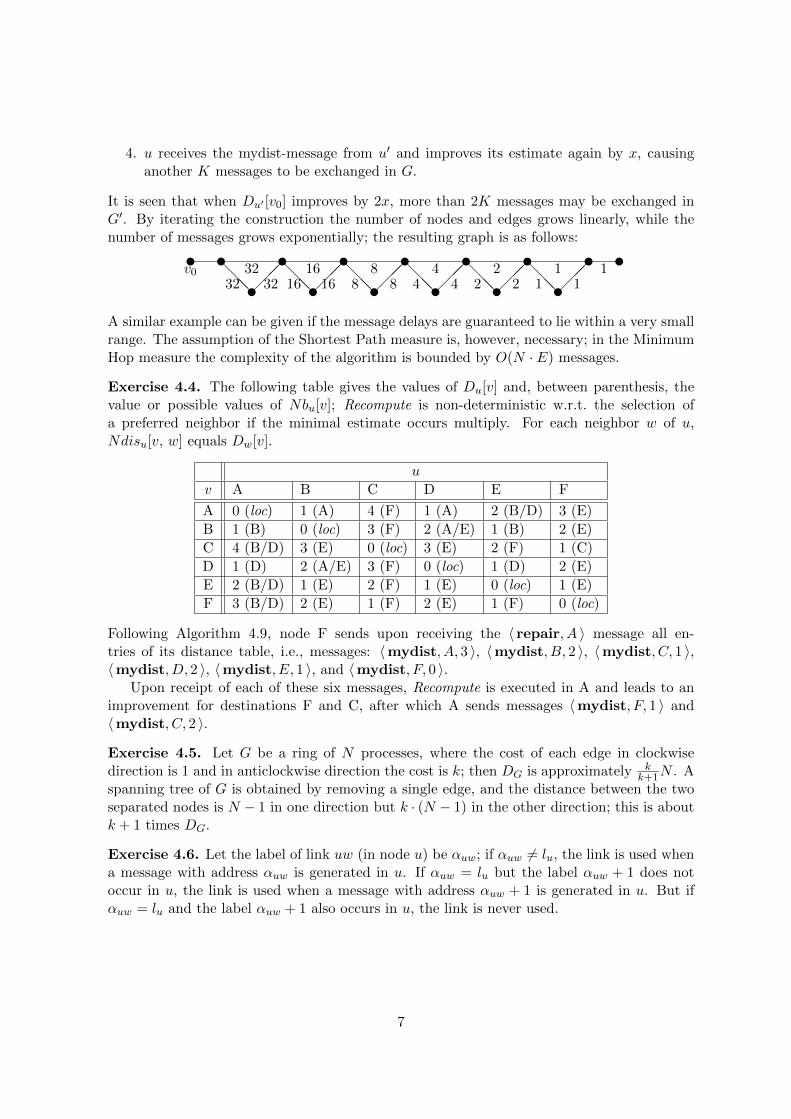
It is seen that when Du′ [v0] improves by 2x, more than 2K messages may be exchanged inG′. By iterating the construction the number of nodes and edges grows linearly, while thenumber of messages grows exponentially; the resulting graph is as follows:u u u u u u u u

u u u u u u@@@�

��@@@�

��@@@�

��@@@�

��@@@�

��@@@�

�� 1u

11

2481632v032 32 16 16 8 8 44 2 2 1

A similar example can be given if the message delays are guaranteed to lie within a very smallrange. The assumption of the Shortest Path measure is, however, necessary; in the MinimumHop measure the complexity of the algorithm is bounded by O(N · E) messages.

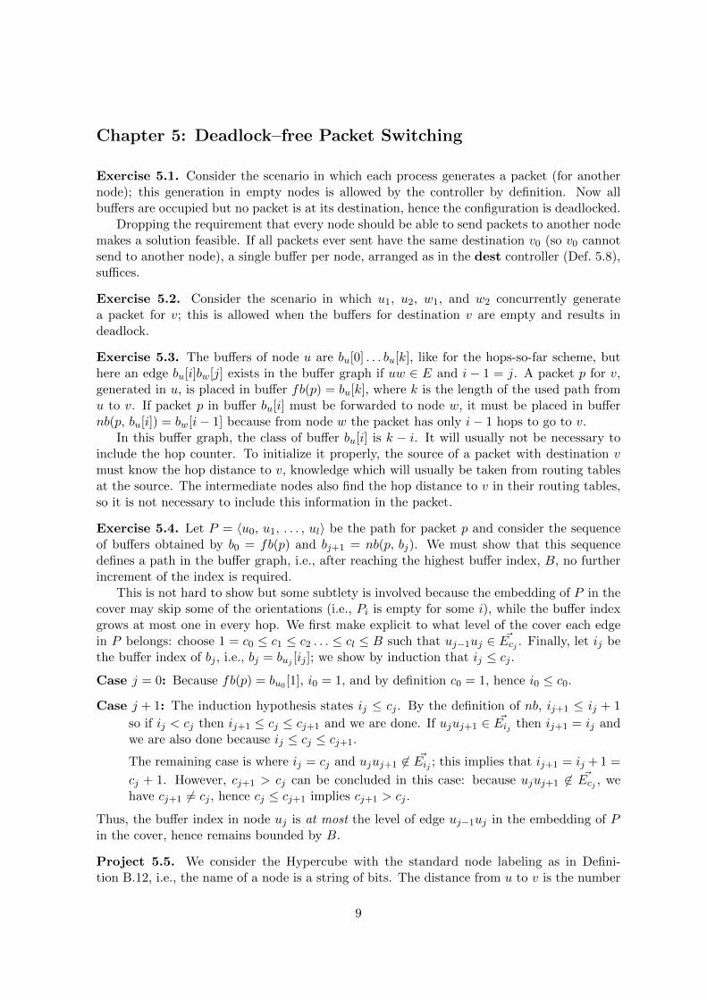
Exercise 4.4. The following table gives the values of Du[v] and, between parenthesis, thevalue or possible values of Nbu[v]; Recompute is non-deterministic w.r.t. the selection ofa preferred neighbor if the minimal estimate occurs multiply. For each neighbor w of u,Ndisu[v, w] equals Dw[v].

u

v A B C D E F

A 0 (loc) 1 (A) 4 (F) 1 (A) 2 (B/D) 3 (E)

B 1 (B) 0 (loc) 3 (F) 2 (A/E) 1 (B) 2 (E)

C 4 (B/D) 3 (E) 0 (loc) 3 (E) 2 (F) 1 (C)

D 1 (D) 2 (A/E) 3 (F) 0 (loc) 1 (D) 2 (E)

E 2 (B/D) 1 (E) 2 (F) 1 (E) 0 (loc) 1 (E)

F 3 (B/D) 2 (E) 1 (F) 2 (E) 1 (F) 0 (loc)

Following Algorithm 4.9, node F sends upon receiving the 〈 repair, A 〉 message all en-tries of its distance table, i.e., messages: 〈mydist, A, 3 〉, 〈mydist, B, 2 〉, 〈mydist, C, 1 〉,〈mydist, D, 2 〉, 〈mydist, E, 1 〉, and 〈mydist, F, 0 〉.

Upon receipt of each of these six messages, Recompute is executed in A and leads to animprovement for destinations F and C, after which A sends messages 〈mydist, F, 1 〉 and〈mydist, C, 2 〉.

Exercise 4.5. Let G be a ring of N processes, where the cost of each edge in clockwisedirection is 1 and in anticlockwise direction the cost is k; then DG is approximately k

k+1N . Aspanning tree of G is obtained by removing a single edge, and the distance between the twoseparated nodes is N − 1 in one direction but k · (N − 1) in the other direction; this is aboutk + 1 times DG.

Exercise 4.6. Let the label of link uw (in node u) be αuw; if αuw 6= lu, the link is used whena message with address αuw is generated in u. If αuw = lu but the label αuw + 1 does notoccur in u, the link is used when a message with address αuw + 1 is generated in u. But ifαuw = lu and the label αuw + 1 also occurs in u, the link is never used.

7

This picture shows an example of an ILS where thisoccurs for the edge 12 on both sides; hence the edge12 is not used for traffic in neither direction. Thescheme is valid.A scheme not using edge uw is not optimal becausetraffic between u and w is sent over two or morehops while d(u, w) = 1.

����

��������..

....

....

....

.0 1

2 3

����

1

1 0

2 2

0 0

3 2

2

Exercise 4.7. Exploit Figure 4.16 to de-sign a detour running through all nodes ofthe network. In this network, such a de-tour is made by messages from u to v. Thenodes marked xi send the message downthe tree via the dotted frond edges becauseyi+1 has a node label between xi+1 and v(both edges are labeled with the node la-bel of the adjacent node).

u uu u uuuuu

uuuuu u uu uu uu u

y4

uuu

��

���

��

@@@@@@@

��

��

���

���

����

���

��

��

��

���

��

....................

....................

....................

u

v

x2

x1

x3

y2

y3

Exercise 4.8. A DFS tree in a ring has depth N − 1; the ILS is as indicated here, and amessage from 0 to N −2 travels via N −2 hops (as does a message in the opposite direction).

� ��� �� � �� � �� � ��..... . . . . . . . . . . . . . . . . . . . . . . . . . . . . . . . . . . . . . . . . . . . . . . . . . . . . . . . . . . . . .....

? ? ? ? ?� �� ?

N − 1

1 2

N − 1 0

3 N − 2 N − 10 0 0 0 N − 2

N − 3 N − 210 2

Exercise 4.9. (1) Besides minimality, the only requirement on T is that it contains all ci;consequently, every leaf of T is one of the ci (otherwise, a leaf could be removed, contradictingminimality).(2) Because a tree has N − 1 edges, the node degrees sum up to 2(N − 1), and leaveshave degree 1. With m leaves, there are N − m nodes with degree at least 2, and thesedegrees sum up to 2N −m− 2; so the number of nodes with degree larger than 2 is at most2N −m− 2− 2(N −m) = m− 2.

8

Chapter 5: Deadlock–free Packet Switching

Exercise 5.1. Consider the scenario in which each process generates a packet (for anothernode); this generation in empty nodes is allowed by the controller by definition. Now allbuffers are occupied but no packet is at its destination, hence the configuration is deadlocked.

Dropping the requirement that every node should be able to send packets to another nodemakes a solution feasible. If all packets ever sent have the same destination v0 (so v0 cannotsend to another node), a single buffer per node, arranged as in the dest controller (Def. 5.8),suffices.

Exercise 5.2. Consider the scenario in which u1, u2, w1, and w2 concurrently generatea packet for v; this is allowed when the buffers for destination v are empty and results indeadlock.

Exercise 5.3. The buffers of node u are bu[0] . . . bu[k], like for the hops-so-far scheme, buthere an edge bu[i]bw[j] exists in the buffer graph if uw ∈ E and i − 1 = j. A packet p for v,generated in u, is placed in buffer fb(p) = bu[k], where k is the length of the used path fromu to v. If packet p in buffer bu[i] must be forwarded to node w, it must be placed in buffernb(p, bu[i]) = bw[i− 1] because from node w the packet has only i− 1 hops to go to v.

In this buffer graph, the class of buffer bu[i] is k − i. It will usually not be necessary toinclude the hop counter. To initialize it properly, the source of a packet with destination vmust know the hop distance to v, knowledge which will usually be taken from routing tablesat the source. The intermediate nodes also find the hop distance to v in their routing tables,so it is not necessary to include this information in the packet.

Exercise 5.4. Let P = 〈u0, u1, . . . , ul〉 be the path for packet p and consider the sequenceof buffers obtained by b0 = fb(p) and bj+1 = nb(p, bj). We must show that this sequencedefines a path in the buffer graph, i.e., after reaching the highest buffer index, B, no furtherincrement of the index is required.

This is not hard to show but some subtlety is involved because the embedding of P in thecover may skip some of the orientations (i.e., Pi is empty for some i), while the buffer indexgrows at most one in every hop. We first make explicit to what level of the cover each edgein P belongs: choose 1 = c0 ≤ c1 ≤ c2 . . . ≤ cl ≤ B such that uj−1uj ∈ ~Ecj . Finally, let ij bethe buffer index of bj , i.e., bj = buj [ij ]; we show by induction that ij ≤ cj .

Case j = 0: Because fb(p) = bu0 [1], i0 = 1, and by definition c0 = 1, hence i0 ≤ c0.

Case j + 1: The induction hypothesis states ij ≤ cj . By the definition of nb, ij+1 ≤ ij + 1

so if ij < cj then ij+1 ≤ cj ≤ cj+1 and we are done. If ujuj+1 ∈ ~Eij then ij+1 = ij andwe are also done because ij ≤ cj ≤ cj+1.

The remaining case is where ij = cj and ujuj+1 6∈ ~Eij ; this implies that ij+1 = ij + 1 =

cj + 1. However, cj+1 > cj can be concluded in this case: because ujuj+1 6∈ ~Ecj , wehave cj+1 6= cj , hence cj ≤ cj+1 implies cj+1 > cj .

Thus, the buffer index in node uj is at most the level of edge uj−1uj in the embedding of Pin the cover, hence remains bounded by B.

Project 5.5. We consider the Hypercube with the standard node labeling as in Defini-tion B.12, i.e., the name of a node is a string of bits. The distance from u to v is the number

9

of positions i with ui 6= vi and an optimal path is obtained by reversing the differing bits inany order.

Now adopt the following routing algorithm. In the first phase, reverse the bits that are1 in u and 0 in v (in any order), then reverse the bits that are 0 in u and 1 in v. Thus, thenumber of 1-bits decreases in the first phase and increases in the second phase. All obtainedpaths are covered by the acyclic orientation cover HC0, HC1, where in HC0 all edges aredirected towards the node with the smaller number of 1’s and in HC1 the other way. Thisshows that deadlock free packet switching is possible with only two buffers per node.

Shortest paths that are all emulated in the cover described here cannot be encoded inan interval labeling scheme. In fact, Flammini demonstrated that the minimal number ofintervals needed globally to represent shortest paths covered by HC0, HC1 is lower boundedby Θ(N

√N), which means that at least

√N/ logN intervals per link (average) are needed.

On the other hand, the cover described above is not the only cover of size two that emulatesa shortest path between every two nodes. Whether shortest paths emulated by another covercan be encoded in an interval labeling scheme is unknown.

Exercise 5.6. We start to prove the correctness of BC. First, if u is empty, fu = B henceB > k implies k − fu < 0, so the acceptance of every packet is allowed.

To show deadlock-freedom of BC, assume γ is a deadlocked configuration and obtain δas in the proof of Theorem 5.17. Let p be a packet in δ that has traveled a maximal numberof hops, i.e., the value of tp is the highest of all packets in δ, and let p reside in u. Node u isnot p’s destination, so let w be the node to which p must be forwarded; as this is move is notallowed there is a packet in w (an empty node accepts every packet). Choose q as the mostrecently accepted one of the packets in w and let f ′w be the number of free buffers in w justbefore acceptance of q; we find f ′w ≤ fw + 1. The acceptance of q implies tq > k− f ′w but therefusal of p implies tp + 1 ≤ k − fw. Consequently,

tq > k − f ′w ≥ k − (fw + 1) ≥ tp,

contradicting the choice of p.

As expected, the correctness of BS is a little bit more intricate. Again, an empty node ac-cepts every packet because

∑jt=0 it−B+k < 0; this shows that generation in (and forwarding

to) empty nodes is allowed and we use it in the proof below.Again, assume a deadlocked configuration γ, and obtain δ as usual; choose p a packet in

γ with maximal value of tp, let u be the node where p resides and w be the node to which pmust be forwarded. Choose q the packet in w that maximizes tq; this choice implies it = 0

for t > tq. Let r be the most recently accepted packet in w, and ~i and ~i′ the state vector ofw in δ, and just before accepting r, respectively.(1) The acceptance of r implies

∀j, tr ≤ j ≤ k : j >

j∑t=0

i′t −B + k.

(2) The choice of r implies that it ≤ i′t for all t 6= ts and itr ≤ i′tr + 1, so we find

∀j, ts ≤ j ≤ k : j >

j∑t=0

it −B + k − 1.

10

(3) In particular, with j = tq:

tq >

tq∑t=0

it −B + k − 1.

(4) Now use that p is not accepted by w, i.e.,

∃j0, tp + 1 ≤ j0 ≤ k : j0 ≤j0∑t=0

it −B + k.

(5) This gives the inequality

tp < tp + 1≤ j0 as chosen in (4)

≤∑j0

t=0 it −B + k from (4)

≤∑k

t=0 it −B + k because it ≥ 0

=∑tq

t=0 it −B + k because it = 0 for t > tq≤ tq, see (3)

which contradicts the choice of p.

Exercise 5.7. Assume the acceptance of packet p by node u is allowed by BC; that is,tp > k − fu. As the path length is bounded by k, sp ≤ k − tp, i.e., sp < k − (k − fu) = fu;consequently the move is allowed by FC.

11

Chapter 6: Wave and Traversal Algorithms

Exercise 6.1. The crux of this exercise lies in the causal dependency between receive andsend in systems with synchronous message passing; a dependency that is enforced withoutpassing a message from the receiver to the sender. Consider a system with two processes pand q; p may broadcast a message with feedback by sending it to q and deciding; completionof the send operation implies that q has received the message when p decides. On the otherhand, it will be clear that p cannot compute the infimum by only sending a message (i.e.,without receiving from q).

The strength of the wave algorithm concept lies in the equivalence of causal chains andmessage chains under asynchronous communications. Hence, the causal dependency requiredfor wave algorithms implies the existence of message chains leading to a decide event andallows infimum computations.

Wave algorithms for synchronous communications can be defined in two ways. First,one may require a causal relation between each process and a decide event; in this case, thedefinition is too weak to allow infimum computation with waves, as is seen from the aboveexample. Second, one may require a message chain from each process to a decide event; inthis case, the definition is too strong to conclude that each PIF algorithm satisfies it, as isalso seen from the example. In either case, however, we lack the full strength of the waveconcept for asynchronous communications.

Exercise 6.2. The proof assumes it is possible to choose j′q such that J ≤ j′q is not satisfied,i.e., that J is not a bottom.

Let X be an order with bottom ⊥. If p has seen a collection of inputs whose infimum is⊥, a decision on ⊥ can safely be made because it follows that ⊥ is the correct output. Nowconsider the following algorithm. Process p receives the inputs of its neighbors and verifieswhether their infimum is ⊥; if so, p decides on ⊥, otherwise a wave algorithm is started and pdecides on its outcome. This algorithm correctly computes the infimum, but does not satisfythe dependency requirement of wave algorithms.

Exercise 6.3. The required orders on the natural numbers are:(1) Define a ≤ b as a divides b.(2) Define a ≤ b as b divides a.The first order has bottom 1, the second has bottom 0.

The required orders on the subsets are:(1) Define a ≤ b as a is a subset of b.(2) Define a ≤ b as b is a subset of a.The first order has bottom ∅, the second has bottom U .

The given solutions are unique; the proof of the Infimum Theorem (see Solution 6.4)reveals that the order ≤? whose infimum function is ? is defined by

a ≤? b ≡ (a ? b) = a.

Exercise 6.4. This exercise is solved by an extensive, but elementary manipulation withaxioms and definitions. Let the commutative, associative, and idempotent operator ? on Xbe given and define a binary relation ≤? by x ≤? y ⇐⇒ (x ? y) = x.

12

We shall first establish (using the assumed properties of ?) that the relation ≤? is a partialorder on X, i.e., that this relation is transitive, antisymmetric and reflexive.

1. Transitivity: Assume x ≤? y and y ≤? z; by definition of ≤?, (x?y) = x and (y?z) = y.Using these and associativity we find (x ? z) = (x ? y) ? z = x ? (y ? z) = x ? y = x, i.e.,x ≤? z.

2. Antisymmetry: Assume x ≤? y and y ≤? x; by definition of ≤?, x ? y = x andy ? x = y. Using these and commutativity we find x = y.

3. Reflexivity: By idempotency, x ? x = x, i.e., x ≤? x.

In a partial order (X, ≤), z is the infimum of x and y w.r.t. ≤ if z is a lower bound, and zis the largest lower bound, i.e., (1) z ≤ x and z ≤ y; and (2) every t with t ≤ x and t ≤ ysatisfies t ≤ z also. We continue to show that x ? y is the infimum of x and y w.r.t. ≤?; letz = x ? y.

1. Lower bound: Expand z and use associativity, commutativity, associativity again,and idempotency to find z ? x = (x ? y) ? x = x ? (y ? x) = x ? (x ? y) = (x ? x) ? y =x ? y = z, i.e., z ≤? x.Expand z and use associativity and idempotency to find z ? y = (x ? y) ? y x ? (y ? y) =x ? y = z, i.e., z ≤? y.

2. Smallest l.b.: Assume t ≤? x and t ≤? y; by definition, t ? x = t and t ? y = t. Then,using these, z = x?y, and associativity, we find t ? z = t ? (x?y) = (t ?x)?y = t ? y = t,i.e., t ≤? z.

In fact, the partial order is completely determined by its infimum operator, i.e., it ispossible to demostrate that ≤? as defined above is the only partial order of which ? is theinfimum operator. This proof is left as a further exercise!

Exercise 6.5. Consider the terminal configuration γ as in the proof of Theorem 6.16. It wasshown there that at least one process has decided; by Lemma 6.4 all other processes havesent, and by the algorithm the process itself has sent, so K = N . Now F , the number of falserec bits, equals N − 2 and each process has either 0 or 1 of them; consequently, exactly twoprocesses have 0 false rec bits.

Exercise 6.6. Each message exchanged in the echo algorithm contains a label (string) anda letter. The initiator is assigned label ε and every non-initiator computes its node labelupon receipt of the first message (from its father), by concatenating the label and the letterin the message. When sending tokens, a process includes its node label, and the letter inthe message is chosen different for each neighbor. In this way the label of each node extendsthe label of its father by one letter, and the labels of the sons of one node are different. Tocompute the link labels, each node assigns to the link to the father the label ε and to allother links the label found in the message received through that link. If a message from theinitiator is received but the initiator is not the father, the node has a frond to the root andrelabels its father link with the label of the father (cf. Definition 4.41).

The labeling can be computed in O(D) time because it is not necessary that a nodewithhelds the message to its father until all other messages have been received (as in theEcho algorithm). In fact, as was pointed out by Erwin Kaspers, it is not necessary to send

13

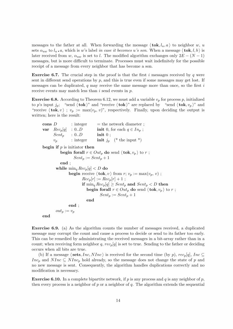
messages to the father at all. When forwarding the message 〈 tok, lu, a 〉 to neighbor w, usets αuw to lu � a, which is w’s label in case it becomes u’s son. When a message 〈 tok, l, b 〉 islater received from w, αuw is set to l. The modified algorithm exchanges only 2E − (N − 1)messages, but is more difficult to terminate. Processes must wait indefinitely for the possiblereceipt of a message from every neighbor that has become a son.

Exercise 6.7. The crucial step in the proof is that the first i messages received by q weresent in different send operations by p, and this is true even if some messages may get lost. Ifmessages can be duplicated, q may receive the same message more than once, so the first ireceive events may match less than i send events in p.

Exercise 6.8. According to Theorem 6.12, we must add a variable vp for process p, initializedto p’s input jp; “send 〈 tok 〉” and “receive 〈 tok 〉” are replaced by “send 〈 tok, vp 〉” and“receive 〈 tok, v 〉 ; vp := max(vp, v)”, respectively. Finally, upon deciding the output iswritten; here is the result:

cons D : integer = the network diameter ;var Recp[q] : 0..D init 0, for each q ∈ Inp ;

Sentp : 0..D init 0 ;vp : integer init jp (* the input *)

begin if p is initiator thenbegin forall r ∈ Outp do send 〈 tok, vp 〉 to r ;

Sentp := Sentp + 1end ;

while minq Recp[q] < D dobegin receive 〈 tok, v 〉 from r; vp := max(vp, v) ;

Recp[r] := Recp[r] + 1 ;if minq Recp[q] ≥ Sentp and Sentp < D then

begin forall r ∈ Outp do send 〈 tok, vp 〉 to r ;Sentp := Sentp + 1

endend ;

outp := vpend

Exercise 6.9. (a) As the algorithm counts the number of messages received, a duplicatedmessage may corrupt the count and cause a process to decide or send to its father too early.This can be remedied by administrating the received messages in a bit-array rather than in acount; when receiving form neighbor q, recp[q] is set to true. Sending to the father or decidingoccurs when all bits are true.

(b) If a message 〈 sets, Inc,NInc 〉 is received for the second time (by p), recp[q], Inc ⊆Incp and NInc ⊆ NIncp hold already, so the message does not change the state of p andno new message is sent. Consequently, the algorithm handles duplications correctly and nomodification is necessary.

Exercise 6.10. In a complete bipartite network, if p is any process and q is any neighbor of p,then every process is a neighbor of p or a neighbor of q. The algorithm extends the sequential

14

polling algorithm (Algorithm 6.10) in the sense that the initiator polls its neighbors, and oneneighbor (q) polls all of its (q’s) neighbors.

The initiator polls its neighbors, but uses a special token for exactly one of its neighbors(for example, the first). The polled processes respond as in Algorithm 6.10, except the processthat receives the special token: it polls all other neighbors before sending the token back tothe originator.

Project 6.11. My conjecture is that the statement is true; if so, it demonstrates that senseof direction “helps” in hypercubes.

Exercise 6.12. In this picture the dotted lines arefronds and p is the root of the tree. The numberswritten at each node indicate the order in whichthe token visits the nodes.Observe that after the third step, when p has re-ceived the token from r, p forwards the token to s,while rules R1 and R2 would allow to send it backto r. This step is a violation of rule R3; of course,R3 must be violated somewhere to obtain a treethat is not DFS.

� ��

� ��� ��

����

@@@@

. . . . . . . . . . . . . . .

� ��

.................

s

0, 3, 7, 10

2, 8

1, 5, 9 4, 6

p

q

r

Exercise 6.13. The node labels are of course computed by a DFS traversal, where the tokencarries a counter that is used as the label and then incremented every time the token visits aprocess for the first time. After such a traversal (with any of the DFS algorithms presentedin Section 6.4) each process knows its father, and which of its neighbors are its sons. Thevalue ku in Definition 4.27 is found as the value of the token that u returns to its father. Noweach node can compute the link labels as in Definition 4.27 if it can obtain the node label ofeach of its neighbors.

In the sequential algorithm (Algorithm 6.14) and the linear time variants (Algorithm 6.15and Algorithm 6.16/6.17) a node sends a message to each of its neighbors after receivingthe token for the first time. In this message the node label can be communicated to everyneighbor, which allows to perform the computation as argued above.

In the linear message DFS algorithm (with neighbors knowledge, Algorithm 6.18) thelabels of neighbors can also be obtained, but at the expense of further increasing the bitcomplexity. In addition to the list of all visited nodes, the token will contain the node label ofevery visited node. If node u has a frond to an ancestor w, then w and its label are containedin the token when u first receives it. If u has a frond to a descendant w, the token containsw and its label when the token returns to u after visiting the subtree containing w. In bothcases u obtains w’s label from the token before the end of the algorithm.

Exercise 6.14. Each process sorts the list of names; the token contains an array of N bits,where bit i is set true if the process whose name has rank i is in the list.

Exercise 6.15. Each message sent upwards in the tree contains the sum over the subtree;the sender can compute this sum because it knows its own input and has received messages(hence sums) from all its subtrees. In order to avoid an explicit distinction between messagesfrom sons (reporting subtree sums) and messages from the father and via fronds (not carryingany relevant information) we put the value 0 in every message not sent upward. Assumingp’s input is given as jp, the program for the initiator becomes:

15

begin forall q ∈ Neighp do send 〈 tok, 0 〉 to q ;

while recp < #Neighp do

begin receive 〈 tok, s 〉 ; jp := jp + s ; recp := recp + 1 end ;Output: jp

end

and for non-initiators:

begin receive 〈 tok, s 〉 from neighbor q ; fatherp := q ; recp := 1 ;

forall q ∈ Neighp, q 6= fatherp do send 〈 tok, 0 〉 to q ;

while recp < #Neighp do

begin receive 〈 tok, s 〉 ; jp := jp + s ; recp := recp + 1 end ;send 〈 tok, jp 〉 to fatherp

end

Non-initiators ignore the value received in the first message; however, this value is not receivedfrom a son and it is always 0.

Exercise 6.17. In the longest message chain it is always the case that the receipt of mi

and the sending of mi+1 occur in the same process. Otherwise, the causal relation betweenthese events is the result of a causal chain containing at least one additional message, andthe message chain can be extended.

The chain time complexity of Algorithm 6.8 is exactly N .First, consider a message chain in any computation. In the algorithm each process sends

to every neighbor, and these sends are not separated by receives in the same process; conse-quently, each message in the chain is sent by a different process. This implies that the lengthof the chain is at most N .

Second, consider an execution on processes p1 through pN where only p1 initiates thealgorithm and the first message received by pi+1 (for i > 1) is the one sent by pi. Thiscomputation contains a message chain of length N .

(The time complexity of the algorithm is 2; because p1 sends a message to all processesupon initialization, all processes are guaranteed to send within one time unit from the start.Indeed, in the execution given above this single message is bypassed by a chain of N − 1messages.)

16

Chapter 7: Election Algorithms

Exercise 7.1. Assume, to the contrary, that process l in network G becomes elected and itschange to the leader state is not preceded by any event in process p. Construct network G′,consisting of two copies of G, with one additional link between the two copies of process p;this is to ensure G′ is connected. In both copies of G′ the relative ordering of identities issimilar to the ordering of the identities in G. Because a comparison algorithm is assumed, thecomputation on G leading to the election of l can be replayed in the two parts of G′, whichresults in a computation in which two processes become leader.

Exercise 7.2. Because 〈wakeup 〉 messages are forwarded immediately by every process, allprocesses have started the tree algorithm withing D time units from the start of the wholealgorithm. It remains to show that the time complexity of the tree algorithm, including theflooding of the answer, is D; assume the tree algorithm is started at time t.

Consider neighbors p and q in the tree; it can be shown by induction that process q sendsa message to p at the latest at time t+depth(Tqp). (Indeed, the induction hypothesis allows toderive that by then q has received from all neighbors other then p. If no message was receivedfrom p the “first” token by q is sent to p, otherwise a “flooding” token is sent.) Consequently,the latest possible time for p to decide is t + 1 + maxq∈Neighp

depth(Tqp), which is at most

t+D (for p a leaf on the diameter path of the tree).

Exercise 7.3. For convenience, write H0 =∑0

j=11j = 0, so

∑mi=1 Hi =

∑mi=0 Hi. Further

observe that Hi =∑i

j=11j = Hm −

∑i<j≤m

1j . Now

∑mi=0 Hi =

∑mi=0

(Hm −

∑i<j≤m

1j

)see above

= (m+ 1)Hm −∑m

i=0

∑i<j≤m

1j

= (m+ 1)Hm −∑m

j=1

∑0≤i<j

1j reverse summations

= (m+ 1)Hm −∑m

j=1 1 because∑

0≤i<j1j = 1 !!

= (m+ 1)Hm −m

Exercise 7.4. This is an example of solving a summation by integration. By drawingrectangles of sizes 1

i in a graph of the function f(x) = 1x it is easily seen that HN >

∫ N+1x=1

dxx =

ln(N + 1). The other bound is shown similarly.

Exercise 7.5. As the token of the winner makes N hops, and each of the remaining N − 1processes initiates a token, which travels at least one hop, the number of messages is at least2N − 1. This number is achieved when each process except the one with smallest identityis followed in the ring by a process with smaller identity, i.e., the identities are “ordered”decreasingly in the message direction (mirror Figure 7.4).

Exercise 7.6. Instead of repeating the argument in the proof of Theorem 7.6, we give thefollowing informal argument.A non-initiator only forwards messages, so the sequence of non-initiators between two succes-sive initiators simulates an asynchronous link between the two initiators. It can thus be seenthat the number of messages sent by initiators is S ·HS on the average.A message sent by an initiator may be forwarded for several hops by non-ititiators before be-

17

ing received by the next initiator; on the average, the number of links between two successiveinitiators is N/S. Consequently, the average complexity is N ·HS .

Exercise 7.7. We first construct the arrangements that yield long executions; if there aretwo processes (N = 21) with identities 1 and 2, the algorithm terminates in two (1 + 1)rounds. Given an arrangement of 2k processes with identities 1 through 2k for which thealgorithm takes k + 1 rounds, place one of the identities 2k + 1 through 2k+1 between eachof the processes in the given arrangement. We obtain an arrangement of 2k+1 processes withidentities 1 through 2k+1 for which the algorithm uses k + 2 rounds.

Assume the arrangement contains two local minima; if both minima and their neighborsinitiate, both minima survive the first round, so no leader is elected in the second round.Hence, to guarantee termination within two rounds the arrangement can have only one localminimum, which means that the identities are arranged as in Figure 7.4. The algorithmterminates in one round if and only if there is a single initiator.

Exercise 7.8. ECR = {(s1, . . . , sk) : 1 < i ≤ k ⇒ s1 < si}.

Exercise 7.9. In the Chang-Roberts algorithm, process p compares a received identity q toits own, while in the extinction algorithm p compares q to the smallest identity p has seen sofar.

A difference would occur if p receives an identity q smaller than its own, but larger thanan identity m received previously. However, this does not occur on the ring if communicationis fifo; p receiving m before q then implies that m is on the path from q to p in the ring,so m purges q’s token before it reaches p. In case of non-fifo communication the extinctionalgorithm may safe some messages over Chang-Roberts.

Exercise 7.10. A connect message sent by a process at level 0 can be sent to a sleepingprocess. Connect messages at higher levels are only sent to processes from which an acceptwas previously received, implying that the addressee is awake. A test message can also besent to a sleeping process.

The other messages are sent via edges of the tree (initiate, report, changeroot) or in replyto another message (accept, reject), both implying that the addressee is awake.

Exercise 7.11. Let the first node wake up at t0, then the last one wakes up no later thant0 +N − 1. By t0 +N all connect messages of level 0 have been received, and going to level 1depends only on propagation of initiate messages through the longest chains that are formed,and completes by t1 = t0 + 2N .

Assume the last node reaches level l before time tl ≤ (5l − 3)N . Each node sends lessthan N test messages, hence has determined its locally least outgoing edge by tl + 2N . Thepropagation of report, changeroot/connect, and initiate messages (for level l + 1) via MSTedges takes less than 3N time, hence by time tl+1 ≤ tl + 5N ≤ (5(l+ 1)− 3)N , all nodes areat level l + 1.

Exercise 7.12. The crux of the exercise is to show that Tarry’s traversal algorithm is anO(x) traversal in this case. Indeed, after 6x− 3 hops the token has visited a planar subgraphwith at least 3x− 1 edges, which implies that the visited subnetwork contains at least x+ 1nodes. The election algorithm is now implied by Theorem 7.24.

Exercise 7.13. Solution 1: Tarry’s traversal algorithm is an O(x) traversal algorithm for the

18

torus, because the degree of each node is bounded by 4. Therefore, after 4x hops the tokenhas traversed at least 2x different edges, implying that x+ 1 nodes were visited. The electionalgorithm is now implied by Theorem 7.24.Solution 2: By Theorem 7.21, election is possible in O(N logN +E) messages; for the torus,E = 2 ·N , which implies an O(N logN) bound.

Exercise 7.14. By Theorem 7.21, election is possible in O(N logN + E) messages; for thehypercube, E = 1

2N logN , which implies an O(N logN) bound.

Exercise 7.15. By Theorem 7.21, election is possible in O(N logN + E) messages; the kbound on the node degrees implies that E ≤ 1

2kN , showing that the GHS algorithm satisfiesthe requirements set in the exercise.The class of networks considered in this exercise is kN -traversable (using Tarry’s algorithm),but applying the KKM algorithm only gives an O(k.N logN) algorithm.

19

Chapter 8: Termination Detection

Exercise 8.1. Process p is active if the guard on an internal or send step is enabled, whichmeans, in Algorithm A.2, if

(#{q : ¬recp[q]} ≤ 1 ∧ ¬sentp) ∨ (#{q : ¬recp[q]} = 0 ∧ ¬decp).

All other states are passive.In Algorithm A.1 these passive states occur exactly when the process is waiting to execute

a receive statement.

Exercise 8.2. The time complexity equals the maximal depth of the computation tree atthe moment termination occurs; this can be seen by quantifying the liveness argument inTheorem 8.5. As only processes are internal nodes, this depth is bounded by N . To showthat this is also a lower bound, observe that the time between termination and its detectionis N when the algorithm is applied to the Ring algorithm (Algorithm 6.2).

Exercise 8.3. Construct the spanning tree in parallel with the basic computation anduse the tree algorithm (Algorithm 6.3) for the detection algorithm. If the spanning tree iscompleted when the basic algorithm terminates, detection occurs within N time, but if thebasic algorithm terminates very fast this modification gives no improvement.

Exercise 8.4. According to P0, all pi with i > t are passive. So, if pj with j ≤ t is activated,P0 is not falsified because the state of all pi with i > t remains unchanged. If pj is activatedby pi with i > t, P0 is false already before the activation, hence it is not falsified.

Exercise 8.5. The basic computation circulates a token, starting from p0, but in the oppositedirection. A process becomes passive after sending the token to its predecessor. A processholding the basic token performs local computations until its predecessor has forwarded thedetection token to it. In this way, the detection token is forwarded (N − 1) times betweenevery two steps of the basic token.

Exercise 8.6. Action Rp becomes:

Rp: { A message 〈mes, c 〉 has arrived at p }begin receive 〈mes, c 〉 ;

if statep = activethen send 〈 ret, c 〉 to p0else begin statep := active ; credp := c end

end

Exercise 8.7. Observe that the process names are exclusively used by a process to recognizewhether it is the initiator of a token it receives; Knowledge of the ring size can be used alter-natively. Tokens carry a hop counter, which is 1 for the first transmission, and incrementedevery time it is forwarded. When a token with hop count N is received (by a quiet process),termination is concluded.

Exercise 8.8. This was done by Michiel van Wezel; see [WT94]. Now try your hands onMattern’s algorithm in [Mat87, Section 6.1].

20

Chapter 9: Anonymous Networks

Exercise 9.1. Algorithm C repeats the subsequent execution of A and B until, according toB, ψ has been established. Explicit termination of A and B is necessary because the processesmust be able to continue (with B, or A, respectively) after termination.

If A establishes ψ with probability P , the expected number of times A is executed by C is1/P ; if the complexity of A and B is known, this allows to compute the expected complexityof C.

Exercise 9.2. If the expected message complexity is K, the probability that the LV algo-rithm exchanges more than K/ε messages is smaller than ε. We obtain an MC algorithm bysimulating the LV algorithm for at least K/ε, but at most a finite number of messages.

Each process continues the execution until it has sent or received K/ε messages. Indeed,with probability 1 − ε or higher, termination with postcondition ψ has occurred before thattime, and the number of overall communication actions is bounded (by N ·K/ε), which showsthe new algorithm is Monte Carlo. (If K depends on network parameters such as the size,these parameters must be known.)

Exercise 9.3. A solution based on Algorithm 9.1 does not meet the time bound mentionedin the exercise, because the time complexity of the echo algorithm is linear. However, thelabeling procedure given in the solution to Exercise 6.6 assigns different names within thebounds.

Exercise 9.4. Each process tries to send to every neighbor and to receive from every neighbor.When a process receives from some neighbor, it it becomes defeated and will thereafter onlyreceive messages. When a process succeeds to send to some neighbor, it keeps trying tosend to and receive from the other neighbors. When a process has sent to every neighbor, itbecomes leader and will thereafter not receive any messages.

At most one process becomes leader because if a process becomes leader, all its neighbors(i.e., all processes) are defeated and will not become leader. At most N − 1 processes becomedefeated because if this many processes are defeated there is no process that can send tothe last process. The algorithm terminates because only finitely many (viz., 1

2N(N − 1))communications can occur; consider a terminal configuration. At least one process is notdefeated; if this process still wants to send, it can do so because all processes are ready toreceive. Consequently, the process has sent to every neighbor and is leader.

Exercise 9.5. Let the input of p be given as ap; the following algorithm terminates afterexchanging at most NE messages, and in the terminal configuration, for every p: bp =maxq aq.

bp := ap ; shout 〈val, bp 〉 ;while true do

begin receive 〈val, b 〉 ;if b > bp then begin bp := b ; shout 〈val, bp 〉 end ;

end

Exercise 9.6. (a) The processes execute the Tree algorithm (Algorithm 6.3), reducing theproblem to election between two processes, namely the two neighbors that send each a mes-

21

sage. These break symmetry by repeatedly exchanging a random bit: if the bits are equal,they continue; if they are different, the process that sent a 1 becomes leader.

(b) No; this can be shown with a symmetry preserving argument like the one used toprove Theorem 9.5.

Exercise 9.7. Both networks depicted in Figure 6.21 have diameter at most 2. Let anydeterministic algorithm be given; by using symmetry arguments as in the proof of Theorem 9.5it is shown that there is an execution in, say, the left network in which every process executesthe same steps. The same sequence of steps, executed by every process in the right network,constitutes an execution of the algorithm in that network. Consequently, the same answercan be found by the processes in the left and in the right network; but as the sizes of thesenetworks are different, the incorrect answer is found in at least one network.

This argument is valid for process and for message terminating algorithms. As the erro-neous execution is finite, the argument shows that any probabilistic algorithm may err withpositive probability of error.

Exercise 9.8. Assume N is composite, i.e., N = k · l for k, l > 1; divide the processes in kgroups of l each. Call a coniguration symmetric if the sequence of l states found in one groupis the same for each group, i.e., si = si+l for each i. If γ is a symmetric configuration inwhich a communication event between pi and pi+1 is enabled, then the same event is enabledbetween pi+l and pi1+l, between pi+2l and pi+1+2l, and so forth. These k events regard disjointpairs of processes (because l ≥ 2), hence the computation can continue with these k events inany order, after which a symmetric configuration is found again. In this way, either an infinitecomputation can be constructed, or a computation terminating in a symmetric configuration;the number of leaders in such a configuration is a multiple of k, hence not 1.

Exercise 9.9. The function f is non-constant (because there exist true as well as false valuedinputs), and hence is not computable by a process terminating algorihm if N is not known(Theorem 9.8).

However, f can be computed by a process terminating algorithm. To this end, eachprocess sends its input to its successor, who will determine if the two input equal. If and onlyif mutual equality holds for all processes, f is true, so the problem of computing f reduces toevaluating the logical AND (Theorem 9.9).

Exercise 9.10. The function g is cyclic, but non-constant, and hence is not computable bya process terminating algorihm (Theorem 9.8).

To show that evaluation of g is also impossible by a message terminating algorithm,consider the rings R4 and R8:

uuu

uu u u

uuuu

����@

@@@�

���@

@@@

������

��PPPPBBBB��������PP

PPBBBB

u2 R8

5

7

11

2

5

7

11

2

5

7

11

R4

22

Assuming there exists a correct algorithm to compute g, there exists an execution, C4 say,of this algorithm on R4 that (message) terminates with result true. Each process in R8 hasneighbors with the same inputs as the neighbors of its counterpart (the unique process inR4 with the same input). Consequently, there exists a computation of the algorithm on R8

in which every process executes the same steps as its counterpart in R4. In particular, thealgorithm (message) terminates with result true.

Exercise 9.11. Because failures are acceptable with small probability, it suffices to executea single phase of the Itai–Rodeh algorithm: each process randomly selects a name from therange [0..U) and verifies, by circulating a token, if its name is minimal. Smaller processesremover token, so if a process receives its own token (hopcount N) it becomes a leader. Byincreasing U the probability that the minimum is not unique (a situation that would lead tothe selection of more than one leader) is made arbitrarily small. The message complexity isat most N2 because each token makes at most N steps.

In its simplest form, this algorithm terminates only in the leader(s); Kees van Kemenadedemonstrated how the leader(s) can process-terminate the other processes, still within N2

messages (worst-case). Each token (as long as it survives) accumulates the number of hopsfrom its initiator to the next process with the same name. When a process becomes leaderand learns that the next process with the same name is h hops away, it sends a terminationsignal for h− 1 hops. These hops do not push the message complexity over N2, because thetokens of the next h− 1 processes were not fully propagated.(The simpler strategy of sending a termination signal to the next leader, i.e., over h hops,generates N2 +N messages in the case all processes draw the same name.)

Exercise 9.12. The processes execute input collection as in Theorem 9.6; process p obtainsa sequence seqp of names, consisting of an enumeration of the names on the ring, starting atp. Because the distribution of identities is non-periodic, the N sequences are different; theunique process whose string is lexicographically maximal becomes elected. (For p this is thecase if and only if seqp is maximal among the cyclic shifts of seqp.)

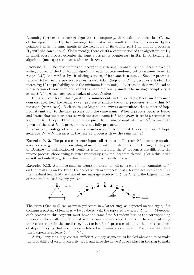
Exercise 9.13. Assuming such an algorithm exists, it will generate a finite computation Con the small ring on the left at the end of which one process, a say, terminates as a leader. Letthe maximal length of the trace of any message received in C be K, and the largest numberof random bits used by any process.

uuuu uu u u u u u u

JJJJ �

�����

�� PPPPQQQQ

�

�

u���

a

bc

a

bc a b c

ab

ca

leader

leaderleader

The steps taken in C can occur in processes in a larger ring, as depicted on the right, if itcontains a pattern of length K+1+3 labeled with the repeated pattern a, b, c, . . .. Moreover,each process in this segment must have the same first L random bits as the correspondingprocess on the small ring. The first K processes execute a strict prefix of the steps taken bytheir counterpart in the small ring, but the last 3 + 1 processes simulate the entire sequenceof steps, implying that two processes labeled a terminate as a leader. The probability thatthis happens is at least 2−(K+3+1).L.

A very large ring may contain sufficiently many segments as labeled above so as to makethe probability of error arbitrarily large, and have the name d at one place in the ring to make

23

it non-periodic. This shows that erroneous behavior of the algorithm is extremely likely, evenin non-periodic rings.

Exercise 9.14. The solution performs input collection and can therefore be used to evalu-ate any cyclic function; it is based on Itai and Rodeh’s algorithm to evaluate the ring size(Algorithm 9.5).

In a test message of Algorithm 9.5 a process includes its input; whenever a process receivesa message with hop count h it learns the input of the process h hops back in the ring. Whenthe algorithm terminates (with common value e of the est variables), each process knows theinputs of the e processes preceding it and evaluates g on this string.

With high probability (as specified in Theorem 9.15) e equals N , and in this case theresult equals the desired value of g.

Exercise 9.15. It is not possible to use Safra’s algorithm, because this algorithm pre-assumesthat a leader (the process named p0 in Algorithm 8.7) is available.

Neither can any other termination detection algorithm be used; it would turn Algo-rithm 9.5 into a process terminating algorithm, but such an algorithm does not exist byTheorem 9.12.

24

Chapter 10: Snapshots

Exercise 10.1. If S∗ is not meaningful there exist p and q and corresponding send/receiveevents s and r such that ap ≺p s and r ≺q aq, which implies ap ≺ aq, so ap 6‖ aq.

Next assume for some p and q, ap ≺ aq; that is, there exists a causal chain from ap toaq. As ap and aq internal but in different processes, the chain contains at least one evente in p following ap, and one event f in q preceding aq. The cut defined by the snapshotincludes f but not e, while e ≺ f ; hence the cut is not consistent, and S∗ is not meaningfulby Theorem 10.5.

Exercise 10.3. The meaningfulness of the snapshot is not guaranteed at all, but by carefuluse of colors meaningless snapshots are recognized and rejected. The snapshot shows a ter-minated configuration if (upon return of the token to p0) mcp0 + q = 0, but this allows callingAnnounce only if in addition c = white and colorp0 = white.

Let m be a postshot message sent by p to q, which is received preshot. The receipt ofthe message colors q black, thus causing q to invalidate the snapshot by coloring the tokenblack as well. Because the receipt of any message colors q black, meaningful snapshots may berejected as well; but termination implies that a terminated snapshot is eventually computedand not rejected.

25

Chapter 12: Synchrony in Networks

Exercise 12.1. If m denotes the contents of the message, the sender computes r = d√me

and s = r2 −m; observe r ≤√m + 1 and s ≤ 2r. The sender sends a 〈 start 〉 message in,

say, pulse i and 〈defr 〉 and 〈defs 〉 messages in pulses i+ r and i+ s, respectively.The receiver counts the number of pulses between the receipt of the 〈 start 〉 and the

〈defr 〉 and 〈defs 〉 messages, thus finding r and s, and “decodes” the message by setting mto r2 − s.

Needless to say, this idea can be generalized to a protocol that transmits the message inO(m1/k) time by sending k + 1 small messages.

Exercise 12.2. Yes, and the proof is similar. The ith process in the segment of the largering goes through the same sequence of states as the corresponding process in the small ring,but up to the ith configuration only.

Exercise 12.3. Assume p receives a j-message from q during pulse i; let σ and τ be the timeof sending and receipt of the message. As the message is received during pulse i,

2iµ ≤ CLOCK (τ)p ≤ 2(i+ 1)µ.

As the message delay is strictly bounded by µ,

2iµ− µ < CLOCK (σ)p ≤ 2(i+ 1)µ.

As the clocks of neighbors differ by less than µ,

2iµ− 2µ < CLOCK (σ)q < 2(i+ 1)µ+ µ.

By the algorithm, the message is sent when CLOCK q = 2jµ, so

2iµ− 2µ < 2jµ < 2(i+ 1)µ+ µ,

which implies i ≤ j ≤ i+ 1.

Exercise 12.4. The time between sending the 〈 start 〉 message and sending an i-messageis exactly 2iµ. Each of the messages incurs a delay of at least 0 but less than µ, so the timebetween the receipt of these messages is between 2iµ− µ and 2iµ+ µ (exclusive).

Exercise 12.6. In all three cases the message is propagated through a suitably chosenspanning tree.

The N -Clique: In the flooding algorithm for the clique, the initiator sends a message to itsN − 1 neighbors in the first pulse, which completes the flooding. The message complexity isN − 1 because every process other than the initiator receives the message exactly once.

The n×n-Torus: In the torus, the message is sent upwards with a hop counter for n−1 steps,so every process in the initiator’s column (except the initiator itself) receives the messageexactly once. Each process in this column (that is, the initiator and every process receivinga message from down) forwards the message to the right through its row, again with a hopcounter and for n − 1 steps. Here every process not in the initiator’s column receives themessages exactly once and from the left. Again, every process except the initiator receivesthe message exactly once.

26

The last process to receive the message is in the row below and the column left of theinitiator; in the (n− 1)th pulse the message receives this row, and only in the 2(n− 1)th pulsethe message is propagated to the end of the row.

The number of pulses can be reduced to 2bn/2c by starting upwards and downwardsfrom the initiator until the messages almost meet, and serve each row also by sending in twodirections. The n-Dimensional Hypercube: The initiator sends a message through its n linksin the first pulse. When receiving a message through link i, a process forwards the messagevia all links < i in the next pulse.

It can be shown by induction on d that a node at distance d from th initiator receivesthe message exactly once, in pulse d, and via the highest dimension in which its node labeldiffers from the initiator. This shows that the message complexity is N − 1 and the numberof pulses is n.

Exercise 12.7. When awaking, the processes initiate a wake-up procedure and then operateas in Section 12.2.1. As a result of the wake-up, the pulses in which processes start theelection may differ by D (the network diameter) but this is compensated for by waiting untilpulse p · (2D) before initiating a flood.

Exercise 12.9. The level of a node equals its distance to the initiator; if d(l, p) = fand q ∈ Neighp, then d(p, q) = 1 and the triangle inequality implies d(l, q) ≥ f − 1 andd(l, q) ≤ f + 1.

27

Chapter 14: Fault Tolerance in Asynchronous Systems

Exercise 14.1. We leave the (quite trivial) correctness proofs of the algorithms as newexercises!

If only termination and agreement are required: Each correct process immediately decideson 0. (This algorithm is trivial because no 1-decision is possible.)

If only termination and non-triviality are required: Each process immediately decides onits input. (Agreement is not satisfied because different decisions can be taken.)

If only agreement and non-triviality are required: Each process shouts its input, then waitsuntil dN+1

2 emessages with the same value have been received, and decides on this value. (Thisalgorithm does not decide in every correct process if insufficiently many processes shout thesame value.)

Exercise 14.2. We leave the (quite trivial) correctness proofs of the algorithms as newexercises!

1. The even parity implies that the entire input can be reconstructed if N − 1 inputs areknown. Solution: Every process shouts its input and waits for the receipt of N − 1values (this includes the process’ own input). The N th value is chosen so as to makethe overall parity even. The process decides on the most frequent input (0 if there is adraw).

2. Solution: Processes r1 and r2 shout their input. A process decides on the first valuereceived.

3. Solution: Each process shouts its input, awaits the receipt of N − 1 values, and decideson the most frequently received value.

Can you generalize these algorithms to be t-crash robust for larger values of t?

Exercise 14.3. As in the proof of Theorem 14.11, two sets of processes S and T can beformed such that the processes in each group decide independently of the other group. Ifone group can reach a decision in which there is a leader, an execution can be constructed inwhich two leaders are elected. If one group can reach a decision in which no leader is elected,an execution can be constructed in which all processes are correct, but no leader is elected.

Exercise 14.4. Choose disjoint subsets S and T of N − t processes and give all processesin S input 1 and the processes in T input 1 + 2ε. The processes in S can reach a decisionon their own; because all inputs in this group are 1, so are the outputs. Indeed, the samesequence of steps is applicable if all processes have input 1, in which case 1 is the only allowedoutput. Similarly, the processes in T decide on output 1 + 2ε on their own. The decisions ofS and T can be taken in the same run, contradicting the agreements requirement.

Exercise 14.5. Write f(s, r) = 12(N − t+ s− 1)(s− (N − t)) + r.

Exercise 14.7. Call the components G1 through Gk. After determining that the decisionvector belongs to Gi, decide on the parity of i.

Exercise 14.8. (1) Sometimes a leader is elected to coordinate a centralized algorithm.Execution of a small number of copies of this algorithm (e.g., in situations where election is

28

not achievable) may still be considerably more efficient than execution by all processes.

(2) The decision vectors of [k, k]-election all have exactly k 1’s, which implies that the taskis disconnected (each node in GT is isolated). The problem is non-trivial because a crashedprocess cannot decide 1; therefore, in each execution the algorithm must decide on a vectorwhere the 1’s are located in correct processes. Consequently, Theorem 14.15 applies.

(3) Every process shouts its identity, awaits the receipt of N − t identities (including its own),and computes its rank r in the set of N − t identities. If r ≤ k+ t then it decides 1, otherwiseit decides 0.

Exercise 14.9. (1) No, it doesn’t. The probability distribution on K defined by Pr[ K ≥k ] = 1/k satisfies limk→∞ Pr[ K ≥ k ] = 0, but yet E[K ] is unbounded.

(2) In all algorithms the probability distribution on the number of rounds K is geometric,i.e., there is a constant c < 1 such that Pr[ (K > k) ] ≤ c ·Pr[ K ≥ k ], which implies thatE[K ] ≤ (1− c)−1.

Exercise 14.10. If all correct processes start round k, at least N − t processes shout in thatround, allowing every correct process to receive N − t messages and finish the round.

Exercise 14.11. (1) In the first round, less than N−t2 processes vote for a value other than

v; this implies that every (correct) process receives a majority of votes for v. Hence in round2 only v-votes are submitted, implying that in round 3 all processes witness for v, and decideon v.

(2) Assuming the processes with input v do not crash, more than N−t2 processes vote for v in

the first round. It is possible that every (correct) process receives all v-votes, and less thanN−t2 votes for the other value. Then in round 2 only v-votes are submitted, implying that in

round 3 all (correct) processes witness for v, and decide on v.

(3) Assuming the processes with input v do not crash, exactly N−t2 processes vote for v in the

first round. In the most favorable (for v) case, all correct processes receive N−t2 v-votes and

N−t2 votes for the other value. As can be seen from Algorithm 14.3, the value 1 is adopted

for the next round in case of a draw. Hence, a decision for v is possible in this case if v = 1.(Of course the choice for 1 in case of draw is arbitrary.)

(4) An initial configurations is bivalent iff the number of 1’s, (#1), satisfies

N − t2≤ #1 <

N + t

2.

Exercise 14.12. (1) In the first round, more than N+t2 correct processes vote for v; this

implies that every correct process accepts a majority of v-votes in the first round, and hencechooses v. As in the proof of Lemma 14.31 it is shown that all correct processes choose vagain in all later rounds, implying that a v-decision will be taken.

(2) As in point (1), in the first round all correct processes choose v in the first round, andvote for it in the second round. Hence, in the second round each correct process accepts atleast N − 2t v-votes; as t < N/5 implies N − 2t > N+t

2 , is follows that in the second roundevery correct process decides on v.

Exercise 14.13. Assume such a protocol exists; partition the processes in three groups, S,T , and U , each of size ≤ t, with the general in S. Let γi be the initial configuration where

29

the general has input v.

Because all processes in U can be faulty, γ0 →S∪T δ0, where in δ0 all processes in S ∪ T havedecided on 0. Similarly, γ1 →S∪U δ1, where in δ1 all processes in S ∪ U have decided on 1.

Now assume the processes in S are all faulty and γ0 is the initial configuration. First theprocesses in S cooperate with the processes in T in such a way that all processes in S∪T decideon 0. Then the processes in S restore their state as in γ1 and cooperate with the processesin U in such a way that all processes in S ∪ U decide on 1. Now the correct processes in Sand U have decided differently, which contradicts the agreement.

Exercise 14.14. At most N initial messages are sent by a correct process, namely by thegeneral (if it is correct). Each correct process shouts at most one echo, counting for Nmessages in each correct process. Each correct process shouts at most two ready messages,counting for 2N messages in each correct process. The number of correct processes can be ashigh as N , resulting in the N · (3N + 1) bound.

(Adapting the algorithm so as to suppress the second sending of ready messages by correctprocesses improves the complexity to N · (2N + 1).)

30

Chapter 15: Fault Tolerance in Synchronous Systems

Exercise 15.1. Denote this number by Mt(N); it is easily seen that M0(N) = N − 1.Further,

Mt(N) = (N − 1) + (N − 1) ·Mt−1(N − 1). (†)

The first term is the initial transmission by the general, the second term represents the N −1recursive calls. The recursion is solved by Mt =

∑ti=0

∏i+1j=1(N − j).

Exercise 15.2. If the decision value is 0 while the general is correct, the general’s input is0 and the discussion in Lemma 15.6 applies. No correct process p initiates or supports anycorrect process, hence the messages sent by p are for supporting a faulty process q; so p shoutsat most t times, which means sending (N − 1).t messages.

If the general is faulty, at most L−1 = t correct processes can initiate without enforcing a1-decision. Correct process p shouts at most 1 〈bm, 1 〉 message, at most t 〈bm, q 〉 messagesfor faulty q, and at most t 〈bm, r 〉 messages for correct r; this means sending at most(N − 1)(2t+ 1) messages.

Exercise 15.3. The faulty processes can send any number of messages, making the totalnumber unbounded; this is why we usually count the number of messages sent by correctprocesses only. Faulty g, p1, p2 could conspire to send 〈val, v 〉 : g : p1 : p2 for many values vto correct p to trap p into sending many messages. Therefore a message that repeats anothermessage’s sequence of signatures is declared invalid.

Then, a correct general sends at most N − 1 messages in pulse 1, and for each sequenceg : p2 : . . . : pi at most N − i messages are sent in pulse i by a process (pi). Thus the numberof messages sent by correct processes is at most

∑t+1i=1

∏ij=1(N − j).

Exercise 15.4. Let p and q be correct; the first and second value accepted by p or q areforwarded, and also accepted by the other. So we let them both receive a third value fromfaulty processes, which is not received by the other:

.......................

.......................

.......................

.......................

HHHHHj

@@@@@R

JJJJJJJ

AAAAAAAAAAU

HHHHHj�

����*

HHHHHj�����* @

@@@@R

@@@@@R

�����

����*

�

����� �

�����

���

��*

�

t is faulty.

������

g

s

t

p

q

Round 1 Round 2 Round 3

d

c

b

a

d

c

a

b

b

aWq = {d, c, a}.

Wp = {c, d, b}.

s is faulty.

g is faulty.

Observe that p and q forward the value c, and d, respectively, in round 2 and that they forwardin round 3 their second received value, namely d, and c, respectively. The third received value(b and a, respectively) is not forwarded in the next round.

Exercise 15.5. The processes achieve interactive consistency on the vector of inputs; thename of p will be the rank of xp in this vector.

Byzantine processes may refuse to participate, but then their default values are assumedto have the higher ranks in the list. They may also cheat by submitting other values than

31

their input, for example, the name of a correct process. Then this name appears multiplyin the list and the correct process decides on the smallest i for which (in the sorted vector)V [i] = xp. Because all correct processes decide on the same vector and this decision vectorcontains the input of each correct process (by dependence), the decisions of correct processesare different and in the range 1 . . . N .

Exercise 15.6. Process q receives signed messages M1 and M2 from p, i.e., the triples(M1, r1, s1) and (M2, r2, s2), where ri = gai mod P and si = (M − d ri)a−1i mod (P − 1).Reuse of a, i.e., a1 = a2 is detected by observing that r1 = r2 in this case. Subtracting s2 froms1 eliminates the unknown term d ri, as s1−s2 = (M1−M2)a

−1, i.e., a = (M1−M2) (s1−s2)−1(mod ()P − 1). Next we find d = (M1 − a s1) r−1.

Exercise 15.7. In rings without zero-divisors, i.e., the axiom a.b = 0⇒ a = 0∨b = 0 applies,a square is the square of at most two elements. Indeed, x2 = z2 reads (x− z)(x+ z) = 0 andhence, by the quoted axiom, x−z = 0 or x+z = 0, i.e., z = x or z = −x. In particular, if p isa prime number, Zp is free of zero-divisors, and x2 = y2 (mod p) implies y = ±x (mod p).

Now let n = p.q be a composit; the ring Zn has zero-divisors because a.b = 0 holds if pdivides a and q divides b, or vice versa. Each square can be the square of up to four numbers;if y = x2, then also y = z2i for

z1 s.t. z1 = x (mod p) and z1 = y (mod q)z2 s.t. z2 = x (mod p) and z2 = −y (mod q)z3 s.t. z3 = −x (mod p) and z3 = y (mod q)z4 s.t. z4 = −x (mod p) and z4 = −y (mod q)

The four numbers form two pairs of opposites: z1 = −z4 and z2 = −z3 and possessing ziand zj such that zi = ±zj is useless. However, if we possess zi and zj from different pairs,compute a = zi + zj and b = zi − zj and observe that neither a nor b equals 0, while a.b = 0.Hence each of a and b is divided by one of p and q, so gcd(a, n) is a non-trivial factor of n.

The square-root box can be used to produce such a pair. Select a random number x anduse the box to produce a square root z of y = x2. Because x was selected randomly, there isa probability of 1

2 that x and y are from different pairs, revealing the factors of n.(The main work in modern factoring methods is spent in finding a non-trivial pair of

numbers with the same square [Len94].)

Exercise 15.8. The clock Cq has ρ-bounded drift, meaning (Eq. 15.1) that its advance inthe real time span t1–t2 (where t2 ≥ t1) differs at most a factor 1 + ρ from t2 − t1, i.e.,

(t2 − t1)(1 + ρ)−1 ≤ Cq(t2)− Cq(t1) ≤ (t2 − t1)(1 + ρ).

This implies that the amount of real time in which the clock advances from T1 to T2 (whereT2 ≥ T1) differs at most a factor 1 + ρ from T2 − T1, i.e.,

(T2 − T1)(1 + ρ)−1 ≤ cq(T2)− cq(T1) ≤ (T2 − T1)(1 + ρ).

Using only the second inequality we find, for any T, T ′:

| cq(T )− cq(T ′) | ≤ (1 + ρ).|T − T ′ |.

32

Consequently, for T = Cp(t) we have

| cq(T )− cp(T ) | = | cq(Cp(t))− cq(Cq(t)) | because Cp(T ) = t = cq(Cq(t))≤ (1 + ρ) . |Cp(t)− Cq(t) | by the bounded drift of cq≤ (1 + ρ) . δ as Cp, Cq are δ − synchronized

at real time t.

Exercise 15.9. Process p asks the server for the time, the server replies immediately witha 〈 time, T 〉 message, and p measures the time I between sending the request and receivingthe reply. As the delay of the 〈 time, T 〉 message was at least I − δmax (this is because atmost δmax of the I time interval was used by the request message) and at most δmax, it differsat most δmax − I/2 from 1

2I. So, p sets its clock to T + 12I , achieving a δmax − I/2 precision;

if ε is smaller than δmax − I/2, the request is repeated.The probability that the delay of the request (or response) message exceeds δmax − ε is

1 − F (δmax − ε), so the probability that both delays exceed δmax − ε is [1 − F (δmax − ε)]2.This implies that the expected number of trials is at most [1 − F (δmax − ε)]−2, hence theexpected number of messages is at most 2.[1 − F (δmax − ε)]−2 and the expected time is atmost 2δmax.[1− F (δmax − ε)]−2.

Exercise 15.10. No, certainly not. Assume N − t processes submit the value x, and inaddition p receives the values x − δ and x + δ. Although at least one of these is erroneous(they differ by more than δ), neither of them is rejected because both have N − t submissionsthat differ δ from it. This lower bounds width(Ap) to 2δ.

33

Chapter 17: Stabilization

Exercise 17.1. The proof resembles that of Theorem 2.17. Consider an execution E =(γ0, γ1, . . .) of S. If E is finite, its last configuration is terminal and belongs to L by (1).Otherwise, consider the sequence (f(γ0), f(γ1), . . .); as there are no infinite decreasing se-quences in W , there is an i such that f(γi) > f(γi+1) does not hold. By (2), γi+1 ∈ L.

Exercise 17.2. In the initial state F is at most 12N(N − 1), and every step of process 0

increases F by at most N − 1 (if it gives privilege to process 1). So the number of steps byprocesses other than 0 before the (N + 1)th step of process 0 is bounded by 1

2N(N − 1) +N(N − 1), which brings the total number of steps to at most 3

2N(N − 1) +N .A suitable norm function is defined as follows [DHS+94, Sec. 6.2]. Call configuration γ

single-segment if there exists j < N such that for all i ≤ j : σi = σ0 and for all i > j : σi 6= σ0.Define

A(γ) =

0 if γ is single segmentthe smallest i s.t.σ0 + i

does not occur in γ otherwise

and W (γ) by W (γ) = N.A(γ) + F (γ). For each step γ → δ, [W (γ) > W (δ) ∨ δ ∈ L] holds.

Exercise 17.4. Modify action (1) so that the idle process p will receive the token only if pand q are oriented differently; if they are oriented the same way, the sending process becomesidle.

Action q p p

(1a)→S

←I −→

→R

(1b)←I

←S −→

←I

Action (1a) is the same silent step as before, but action (1b) will kill the token where originallyit would be forwarded to a process that already has the same orientation. This ensures thattoken circulation ceases, yet we are still guaranteed to have tokens as long as the ring is notlegitimate (by Proposition 17.9).

Exercise 17.6. Replace the variable pref p by a three-valued variable cpq for each neighborq, with value you if p has selected q, other if p has selected r 6= q, and none if p has not madea selection. These variables satisfy a local consistency:

lc(p) ≡ (∀q ∈ Neighp : cpq = none)

∨ (∃q ∈ Neighp : cpq = you ∧ ∀r 6= q ∈ Neighp : cpr = other).

An additional “clearing” action Cp, executed at most once for every process, establishes localconsistency. Quantifications below run over Neighp.

var cpq : (you, other , none);

Cp: { ¬lc(p) }forall q do cpq := none

Mp: { lc(p) ∧ cpq = none ∧ cqp = you }forall r do cpr := other ; cqp := you

Sp: { lc(p) ∧ cpq = cqp = none ∧ ∀r 6= q : crp 6= you

34

forall r do cpr := other ; cqp := you

Up: { lc(p) ∧ cpq = you ∧ cqp = other }forall r do cpr := none

Each process is locally consistent after at most one step, and the algorithm then behaves likethe original one.

Can you prove a bound on length of an execution? Can you modify the algorithm so asto work for the link-register read-one model?

Exercise 17.7. In each matching step (action Mp) the value of c+f+w decreases by at least2, and the other steps decrease the value of the second component of F . Hence the functionF = (b(c+ f +w)/2c, 2c+ f) is also a norm, and proves stabilization within N2 + 21

2N steps.To show the lower bound we inductively construct an execution of 1

2k2 steps on a clique

containing k (even) free processes; if k = 2 the two remaining processes are matched in twosteps. If there are k > 2 free processes p1 and p2, first processes p1 through pk−1 select pk,then process pk matches pk−1, and finally processes p1 through pk−2 unchain from pk. Afterthese 2k − 2 steps the network contains k − 2 free processes, so by induction the executioncan be continued for another 1

2(k − 2)2 steps.A more precise analysis is found in [Tel94]. A proof of stabilization within O(|E|) steps

is found in [DHS+94, Section 7.2].

Exercise 17.8. Assume the state read-all model and have a boolean misp for each p, indi-cating if p is currently in the set M . There are two actions: (1) if both p and a neighborare in M , misp := false; (2) if neither p nor any neighbor is in M , misp := true. Call pblack if (1) applies, gray if (2) applies, and white if neither applies. Action (1) makes theblack process white without making any other process black (a white neighbor could becomegray) and action (2) makes a gray process white without darkening any other process. Sothe pair formed by the numbers of black and gray processes decreases lexicographically withevery step and after less than N2 steps a terminal configuration is reached. In a terminalconfiguration no two neighbors are in M , and every node not in M has a neighbor in M ,hence M is a maximal independent set.

Project 17.10. An outerplanar graph has a node of degree two or less; now re-read pages 538through 540, replacing “six” by “three” and “five” by “two”.

Exercise 17.12. Let the cost of π = 〈p0, . . . , pk〉 be the pair (p0, k). Ordering is lexico-graphically, but to get length increase, paths of length N or longer are larger than paths oflength below N .

Exercise 17.13. When a spanning tree is known, the size is computed by summation persubtree, i.e., each node assigns its count the sum of the counts of its children plus one.Construction of a spanning tree without a priory knowledge of the network size was solvedby Dolev [Dol93].

Exercise 17.14. The update algorithm can compute the longest upward path for each nodewith the following choice of c, f , and the order. Let cp = 0 for each process p, and letfpq(x) = x + 1 if p is the father of q and −∞ otherwise; the order is reversed, i.e., longerpaths are smaller than short ones.

35

Appendix B: Graphs and Networks

Exercise B.1. To prove the first part, select a node v0; because the graph is connected everynode has a finite distance to v0. Sort the remaining nodes as v1 through vN−1 in increasingorder of distance, i.e., i > j ⇒ d(vi, v0) ≤ d(vj , v0). For each of the vi, i > 0, a shortest pathfrom vi to v0 exists; the higher-numbered endpoint of the first edge is vi; hence the numberof edges is at least N − 1.

To show the second part we demonstrate that an acyclic graph contains at least onenode with degree 1 or less; otherwise an infinite path without selfloops could be created,unavoidably hitting a node occuring earlier in the path and revealing a cycle. Then the proofis completed by induction; an acyclic graph on one node has degree 0, and removing a degree-0 or degree-1 node from an acyclic graph reduces the number of nodes, keeping the graphacyclic.

Exercise B.2. Let G = (V, E) be an undirected graph. Assume G is bipartite; fix on aparticular coloring and consider a cycle. As adjacent nodes in the cycle are also adjacent inG, they are colored differently, hence the cycle is of even length.

Now assume G has no odd-length cycles. Select an arbitrary node v0 (or, if G is notconnected: select a node in each connected component) and color node v red if d(v0, v) isodd and black if d(v0, v) is even. Let v and v′ be adjacent nodes, π be any path from v0 tov and π′ any path from v′ to v0. The cycle formed by concatenating π, edge vv′, and π′ haseven length, showing that the lengths of π and π′ have different parity. In particular, d(v0, v)and d(v0, v

′) have different parity, and v and v′ have different colors.

Exercise B.3. A ring of even length has no odd-length cycle and a tree has no cycle at all;use Exercise B.2. In the hypercube, consider a particular node labeling as in Definition B.12and color node v red if the number of 1’s in the label is even and black otherwise. As thelabels of adjacent nodes differ in exactly one bit, their parity is different.

Exercise B.4. Theorem B.4 is Theorem 5.2 of Cormen et al. [CLR90]; I won’t bother tocopy the proof here.

Exercise B.6. A clique on N nodes has (N − 1)! different labelings that are a sense ofdirection. Select a node v0 and observe that the N − 1 different labels can bearranged inexactly (N − 1)! different ways on the edges incident to v0.

1. Each arrangement can be extended to a (unique) sense of direction as follows. Thearrangement defines Lv0(w) for all w 6= v0; set L(w, v0) = N − Lv0(w) and Lu(w) =Lv0(w)− Lv0(u) mod N for u, w 6= v0.

To show that L is a sense of direction, label node v0 with 0 and node w 6= v0 withLv0(w); the obtained node labeling witnesses that L is an orientation.

The (N − 1)! labelins are all different, because they already differ in their projection onv0. Consequently, there are at least (N − 1)! different senses of direction.

2. Each sense of direction L has a different projection on v0; indeed, Lw(v0) = N −Lv0(w)and Lu(w) = Lv0(w)− Lv0(u) mod N can be shown by reasoning with a node labelingwitnessing that L is a sense of direction. Consequently, there are at most (N − 1)!different senses of direction.

36

A hypercube of dimension n has n! different labelings that are a sense of direction. Selecta node v0 and observe that the n different labels can be arranged in exactly n! different wayson the edges incident to v0.

For edges e = (u, v) and f = (w, x), define e and f to be parallel iff d(u, w) = d(v, x)and d(u, x) = d(v, w). Reasoning with a witnessing node labeling it is shown that the labelsof e and f in a sense of direction are equal if and only if e and f are parallel. Furthermore,for each edge f in the hypercube there is exactly one edge e incident to v0 such that e and fare parallel. This shows that, like it is the case for cliques, the entire labeling is defined bythe labeling of the edges of a single node.

Exercise B.7. Assume (1). By the definition of an orientation there exists a labeling N ofthe nodes such that Lu(v) = N (v) − N (u). Using induction on the path, it is easily shownthat Sum(P ) = N (vk)−N (v0). As labels are from the set {1, .., N − 1}, Lu(v) 6= 0, and allnode labels are different. It now follows that v0 = vk if and only if Sum(P ) = 0.

Assume (2). Pick an arbitrary node v0, setN (v0) = 0 and for all u 6= v0 setN (u) = Lv0(u).It remains to show that this node labeling satisfies the constraints in the definition of anorientation. That is, for all nodes u1 and u2, Lu1(u2) = N (u2) − N (u1). For u 6= v0, noteN (v0) = 0 and N (u) = Lv0(u) so Lv0(u) = N (u) − N (v0). As P = v0, u, v0 is closed,Sum(P ) = 0, hence Lu(v0) = −Lv0(u) = N (v0)−N (u). For u1, u2 6= v0, as P = v0, u1, u2, v0is closed, Sum(P ) = 0 and hence Lu1(u2) = −Lv0(u1)−Lu2(v0) = (N (u1)−N (v0))−(N (v0)−N (u2)) = N (u2)−N (u1).

A discussion of the equivalence and similar results for the torus and hypercube are foundin [Tel91].

37

References

[CLR90] Cormen, T. H., Leiserson, C. E., and Rivest, R. L. Introduction to Algo-rithms. McGraw-Hill/MIT Press, 1990 (1028 pp.).

[DHS+94] Dijkhuizen, G. H., Herman, T., Siemelink, W. G., Tel, G., and Verweij,A. Developments in distributed algorithms. Course notes, Dept Computer Science,Utrecht University, The Netherlands, 1994.

[Dol93] Dolev, S. Optimal time self-stabilization in dynamic systems. In proc. Int.Workshop on Distributed Algorithms (Lausanne, 1993), A. Schiper (ed.), vol. 725of Lecture Notes in Computer Science, Springer-Verlag, pp. 160–173.

[Len94] Lenstra, A. Factoring. In proc. 8th Int. Workshop on Distributed Algorithms(Terschelling (NL), 1994), G. Tel and P. Vitanyi (eds.), vol. 857 of Lecture Notesin Computer Science, Springer-Verlag, pp. 28–38.

[Mat87] Mattern, F. Algorithms for distributed termination detection. Distributed Com-puting 2, 3 (1987), 161–175.

[Mat89] Mattern, F. Virtual time and global states of distributed systems. In proc. Par-allel and Distributed Algorithms (1989), M. Cosnard et al. (eds.), Elsevier SciencePublishers, pp. 215–226.

[Tel91] Tel, G. Network orientation. Tech. rep. RUU–CS–91–8, Dept Computer Science,Utrecht University, The Netherlands, 1991. Anon. ftp from ftp.cs.ruu.nl file/pub/RUU/CS/techreps/CS-1991/1991-08.ps.gz.

[Tel94] Tel, G. Maximal matching stabilizes in quadratic time. Inf. Proc. Lett. 49, 6(1994), 271–272.

[Tel00] Tel, G. Introduction to Distributed Algorithms, 2nd edition. Cambridge Univer-sity Press, 2000 (596 pp.).

[WT94] Wezel, M. C. van and Tel, G. An assertional proof of Rana’s algorithm. Inf.Proc. Lett. 49, 5 (1994), 227–233.

38