introduction to differential...
TRANSCRIPT

Introduction to DifferentialEquations
Lecture notes for MATH 2351/2352
(formerly MATH 150/151)
Jeffrey R. Chasnov
The Hong Kong University ofScience and Technology

The Hong Kong University of Science and TechnologyDepartment of MathematicsClear Water Bay, Kowloon
Hong Kong
Copyright c○ 2009–2012 by Jeffrey Robert Chasnov
This work is licensed under the Creative Commons Attribution 3.0 Hong Kong License.
To view a copy of this license, visit http://creativecommons.org/licenses/by/3.0/hk/
or send a letter to Creative Commons, 171 Second Street, Suite 300, San Francisco,
California, 94105, USA.

Preface
What follows are my lecture notes for Math 2351/2352: Introduction to or-dinary differential equations/Differential equations and applications, taught atthe Hong Kong University of Science and Technology. Math 2351, with twolecture hours per week, is primarily for non-mathematics majors and is requiredby several engineering and science departments; Math 2352, with three lecturehours per week, is primarily for mathematics majors and is required for appliedmathematics students.
Included in these notes are links to short tutorial videos posted on YouTube.There are also some links to longer videos of in-class lectures. It is hoped thatfuture editions of these notes will more seamlessly join the video tutorials withthe text.
Much of the material of Chapters 2-6 and 8 has been adapted from thetextbook “Elementary differential equations and boundary value problems” byBoyce & DiPrima (John Wiley & Sons, Inc., Seventh Edition, c○2001). Manyof the examples presented in these notes may be found in this book, and Iapologize to the authors and publisher, with hope that I have not violatedany copyright laws. The material of Chapter 7 is adapted from the textbook“Nonlinear dynamics and chaos” by Steven H. Strogatz (Perseus Publishing,c○1994).
All web surfers are welcome to download these notes, watch the YouTubevideos, and to use the notes and videos freely for teaching and learning. Iwelcome any comments, suggestions or corrections sent by email [email protected].
iii


Contents
0 A short mathematical review 1
0.1 The trigonometric functions . . . . . . . . . . . . . . . . . . . . . 1
0.2 The exponential function and the natural logarithm . . . . . . . 1
0.3 Definition of the derivative . . . . . . . . . . . . . . . . . . . . . 2
0.4 Differentiating a combination of functions . . . . . . . . . . . . . 2
0.4.1 The sum or difference rule . . . . . . . . . . . . . . . . . . 2
0.4.2 The product rule . . . . . . . . . . . . . . . . . . . . . . . 2
0.4.3 The quotient rule . . . . . . . . . . . . . . . . . . . . . . . 2
0.4.4 The chain rule . . . . . . . . . . . . . . . . . . . . . . . . 3
0.5 Differentiating elementary functions . . . . . . . . . . . . . . . . 3
0.5.1 The power rule . . . . . . . . . . . . . . . . . . . . . . . . 3
0.5.2 Trigonometric functions . . . . . . . . . . . . . . . . . . . 3
0.5.3 Exponential and natural logarithm functions . . . . . . . 3
0.6 Definition of the integral . . . . . . . . . . . . . . . . . . . . . . . 3
0.7 The fundamental theorem of calculus . . . . . . . . . . . . . . . . 4
0.8 Definite and indefinite integrals . . . . . . . . . . . . . . . . . . . 5
0.9 Indefinite integrals of elementary functions . . . . . . . . . . . . . 5
0.10 Substitution . . . . . . . . . . . . . . . . . . . . . . . . . . . . . . 6
0.11 Integration by parts . . . . . . . . . . . . . . . . . . . . . . . . . 6
0.12 Taylor series . . . . . . . . . . . . . . . . . . . . . . . . . . . . . . 7
0.13 Complex numbers . . . . . . . . . . . . . . . . . . . . . . . . . . 8
1 Introduction to odes 11
1.1 The simplest type of differential equation . . . . . . . . . . . . . 11
2 First-order odes 13
2.1 The Euler method . . . . . . . . . . . . . . . . . . . . . . . . . . 13
2.2 Separable equations . . . . . . . . . . . . . . . . . . . . . . . . . 14
2.3 Linear equations . . . . . . . . . . . . . . . . . . . . . . . . . . . 17
2.4 Applications . . . . . . . . . . . . . . . . . . . . . . . . . . . . . . 20
2.4.1 Compound interest with deposits or withdrawals . . . . . 20
2.4.2 Chemical reactions . . . . . . . . . . . . . . . . . . . . . . 21
2.4.3 The terminal velocity of a falling mass . . . . . . . . . . . 23
2.4.4 Escape velocity . . . . . . . . . . . . . . . . . . . . . . . . 24
2.4.5 The logistic equation . . . . . . . . . . . . . . . . . . . . . 26
v

vi CONTENTS
3 Second-order odes, constant coefficients 29
3.1 The Euler method . . . . . . . . . . . . . . . . . . . . . . . . . . 29
3.2 The principle of superposition . . . . . . . . . . . . . . . . . . . . 30
3.3 The Wronskian . . . . . . . . . . . . . . . . . . . . . . . . . . . . 30
3.4 Homogeneous odes . . . . . . . . . . . . . . . . . . . . . . . . . . 31
3.4.1 Real, distinct roots . . . . . . . . . . . . . . . . . . . . . . 32
3.4.2 Complex conjugate, distinct roots . . . . . . . . . . . . . 34
3.4.3 Repeated roots . . . . . . . . . . . . . . . . . . . . . . . . 36
3.5 Inhomogeneous odes . . . . . . . . . . . . . . . . . . . . . . . . . 38
3.6 First-order linear inhomogeneous odes revisited . . . . . . . . . . 41
3.7 Resonance . . . . . . . . . . . . . . . . . . . . . . . . . . . . . . . 42
3.8 Damped resonance . . . . . . . . . . . . . . . . . . . . . . . . . . 45
4 The Laplace transform 47
4.1 Definition and properties . . . . . . . . . . . . . . . . . . . . . . . 47
4.2 Solution of initial value problems . . . . . . . . . . . . . . . . . . 51
4.3 Heaviside and Dirac delta functions . . . . . . . . . . . . . . . . . 54
4.3.1 Heaviside function . . . . . . . . . . . . . . . . . . . . . . 54
4.3.2 Dirac delta function . . . . . . . . . . . . . . . . . . . . . 56
4.4 Discontinuous or impulsive terms . . . . . . . . . . . . . . . . . . 57
5 Series solutions 61
5.1 Ordinary points . . . . . . . . . . . . . . . . . . . . . . . . . . . . 61
5.2 Regular singular points: Euler equations . . . . . . . . . . . . . . 65
5.2.1 Real, distinct roots . . . . . . . . . . . . . . . . . . . . . . 67
5.2.2 Complex conjugate roots . . . . . . . . . . . . . . . . . . 67
5.2.3 Repeated roots . . . . . . . . . . . . . . . . . . . . . . . . 67
6 Systems of equations 69
6.1 Determinants and the eigenvalue problem . . . . . . . . . . . . . 69
6.2 Coupled first-order equations . . . . . . . . . . . . . . . . . . . . 71
6.2.1 Two distinct real eigenvalues . . . . . . . . . . . . . . . . 71
6.2.2 Complex conjugate eigenvalues . . . . . . . . . . . . . . . 75
6.2.3 Repeated eigenvalues with one eigenvector . . . . . . . . . 77
6.3 Normal modes . . . . . . . . . . . . . . . . . . . . . . . . . . . . 79
7 Bifurcation theory 83
7.1 Fixed points and stability . . . . . . . . . . . . . . . . . . . . . . 83
7.2 One-dimensional bifurcations . . . . . . . . . . . . . . . . . . . . 87
7.2.1 Saddle-node bifurcation . . . . . . . . . . . . . . . . . . . 87
7.2.2 Transcritical bifurcation . . . . . . . . . . . . . . . . . . . 88
7.2.3 Supercritical pitchfork bifurcation . . . . . . . . . . . . . 88
7.2.4 Subcritical pitchfork bifurcation . . . . . . . . . . . . . . 89
7.2.5 Application: a mathematical model of a fishery . . . . . . 92
7.3 Two-dimensional bifurcations . . . . . . . . . . . . . . . . . . . . 94
7.3.1 Supercritical Hopf bifurcation . . . . . . . . . . . . . . . . 94
7.3.2 Subcritical Hopf bifurcation . . . . . . . . . . . . . . . . . 95
CONTENTS vii
8 Partial differential equations 978.1 Derivation of the diffusion equation . . . . . . . . . . . . . . . . . 978.2 Derivation of the wave equation . . . . . . . . . . . . . . . . . . . 988.3 Fourier series . . . . . . . . . . . . . . . . . . . . . . . . . . . . . 1008.4 Fourier cosine and sine series . . . . . . . . . . . . . . . . . . . . 1028.5 Solution of the diffusion equation . . . . . . . . . . . . . . . . . . 104
8.5.1 Homogeneous boundary conditions . . . . . . . . . . . . . 1048.5.2 Inhomogeneous boundary conditions . . . . . . . . . . . . 1088.5.3 Pipe with closed ends . . . . . . . . . . . . . . . . . . . . 109
8.6 Solution of the wave equation . . . . . . . . . . . . . . . . . . . . 1128.6.1 Plucked string . . . . . . . . . . . . . . . . . . . . . . . . 1128.6.2 Hammered string . . . . . . . . . . . . . . . . . . . . . . . 1148.6.3 General initial conditions . . . . . . . . . . . . . . . . . . 114
8.7 The Laplace equation . . . . . . . . . . . . . . . . . . . . . . . . 1158.7.1 Dirichlet problem for a rectangle . . . . . . . . . . . . . . 1158.7.2 Dirichlet problem for a circle . . . . . . . . . . . . . . . . 116

viii CONTENTS

Chapter 0
A short mathematicalreview
A basic understanding of calculus is required to undertake a study of differentialequations. This zero chapter presents a short review.
0.1 The trigonometric functions
The Pythagorean trigonometric identity is
sin2 𝑥+ cos2 𝑥 = 1,
and the addition theorems are
sin(𝑥+ 𝑦) = sin(𝑥) cos(𝑦) + cos(𝑥) sin(𝑦),
cos(𝑥+ 𝑦) = cos(𝑥) cos(𝑦)− sin(𝑥) sin(𝑦).
Also, the values of sin𝑥 in the first quadrant can be remembered by the rule ofquarters, with 0∘ = 0, 30∘ = 𝜋/6, 45∘ = 𝜋/4, 60∘ = 𝜋/3, 90∘ = 𝜋/2:
sin 0∘ =
√0
4, sin 30∘ =
√1
4, sin 45∘ =
√2
4,
sin 60∘ =
√3
4, sin 90∘ =
√4
4.
The following symmetry properties are also useful:
sin(𝜋/2− 𝑥) = cos𝑥, cos(𝜋/2− 𝑥) = sin𝑥;
andsin(−𝑥) = − sin(𝑥), cos(−𝑥) = cos(𝑥).
0.2 The exponential function and the naturallogarithm
The transcendental number 𝑒, approximately 2.71828, is defined as
𝑒 = lim𝑛→∞
(1 +
1
𝑛
)𝑛
.
1

2 CHAPTER 0. A SHORT MATHEMATICAL REVIEW
The exponential function exp (𝑥) = 𝑒𝑥 and natural logarithm ln𝑥 are inversefunctions satisfying
𝑒ln 𝑥 = 𝑥, ln 𝑒𝑥 = 𝑥.
The usual rules of exponents apply:
𝑒𝑥𝑒𝑦 = 𝑒𝑥+𝑦, 𝑒𝑥/𝑒𝑦 = 𝑒𝑥−𝑦, (𝑒𝑥)𝑝 = 𝑒𝑝𝑥.
The corresponding rules for the logarithmic function are
ln (𝑥𝑦) = ln𝑥+ ln 𝑦, ln (𝑥/𝑦) = ln𝑥− ln 𝑦, ln𝑥𝑝 = 𝑝 ln𝑥.
0.3 Definition of the derivative
The derivative of the function 𝑦 = 𝑓(𝑥), denoted as 𝑓 ′(𝑥) or 𝑑𝑦/𝑑𝑥, is definedas the slope of the tangent line to the curve 𝑦 = 𝑓(𝑥) at the point (𝑥, 𝑦). Thisslope is obtained by a limit, and is defined as
𝑓 ′(𝑥) = limℎ→0
𝑓(𝑥+ ℎ)− 𝑓(𝑥)
ℎ. (1)
0.4 Differentiating a combination of functions
0.4.1 The sum or difference rule
The derivative of the sum of 𝑓(𝑥) and 𝑔(𝑥) is
(𝑓 + 𝑔)′ = 𝑓 ′ + 𝑔′.
Similarly, the derivative of the difference is
(𝑓 − 𝑔)′ = 𝑓 ′ − 𝑔′.
0.4.2 The product rule
The derivative of the product of 𝑓(𝑥) and 𝑔(𝑥) is
(𝑓𝑔)′ = 𝑓 ′𝑔 + 𝑓𝑔′,
and should be memorized as “the derivative of the first times the second plusthe first times the derivative of the second.”
0.4.3 The quotient rule
The derivative of the quotient of 𝑓(𝑥) and 𝑔(𝑥) is(𝑓
𝑔
)′
=𝑓 ′𝑔 − 𝑓𝑔′
𝑔2,
and should be memorized as “the derivative of the top times the bottom minusthe top times the derivative of the bottom over the bottom squared.”

0.5. DIFFERENTIATING ELEMENTARY FUNCTIONS 3
0.4.4 The chain rule
The derivative of the composition of 𝑓(𝑥) and 𝑔(𝑥) is(𝑓(𝑔(𝑥)
))′= 𝑓 ′(𝑔(𝑥)) · 𝑔′(𝑥),
and should be memorized as “the derivative of the outside times the derivativeof the inside.”
0.5 Differentiating elementary functions
0.5.1 The power rule
The derivative of a power of 𝑥 is given by
𝑑
𝑑𝑥𝑥𝑝 = 𝑝𝑥𝑝−1.
0.5.2 Trigonometric functions
The derivatives of sin𝑥 and cos𝑥 are
(sin𝑥)′ = cos𝑥, (cos𝑥)′ = − sin𝑥.
We thus say that “the derivative of sine is cosine,” and “the derivative of cosineis minus sine.” Notice that the second derivatives satisfy
(sin𝑥)′′ = − sin𝑥, (cos𝑥)′′ = − cos𝑥.
0.5.3 Exponential and natural logarithm functions
The derivative of 𝑒𝑥 and ln𝑥 are
(𝑒𝑥)′ = 𝑒𝑥, (ln𝑥)′ =1
𝑥.
0.6 Definition of the integral
The definite integral of a function 𝑓(𝑥) > 0 from 𝑥 = 𝑎 to 𝑏 (𝑏 > 𝑎) is definedas the area bounded by the vertical lines 𝑥 = 𝑎, 𝑥 = 𝑏, the x-axis and the curve𝑦 = 𝑓(𝑥). This “area under the curve” is obtained by a limit. First, the area isapproximated by a sum of rectangle areas. Second, the integral is defined to bethe limit of the rectangle areas as the width of each individual rectangle goes tozero and the number of rectangles goes to infinity. This resulting infinite sumis called a Riemann Sum, and we define∫ 𝑏
𝑎
𝑓(𝑥)𝑑𝑥 = limℎ→0
𝑁∑𝑛=1
𝑓(𝑎+ (𝑛− 1)ℎ
)· ℎ, (2)
where 𝑁 = (𝑏 − 𝑎)/ℎ is the number of terms in the sum. The symbols on theleft-hand-side of (2) are read as “the integral from 𝑎 to 𝑏 of f of x dee x.” The

4 CHAPTER 0. A SHORT MATHEMATICAL REVIEW
Riemann Sum definition is extended to all values of 𝑎 and 𝑏 and for all valuesof 𝑓(𝑥) (positive and negative). Accordingly,
∫ 𝑎
𝑏
𝑓(𝑥)𝑑𝑥 = −∫ 𝑏
𝑎
𝑓(𝑥)𝑑𝑥 and
∫ 𝑏
𝑎
(−𝑓(𝑥))𝑑𝑥 = −∫ 𝑏
𝑎
𝑓(𝑥)𝑑𝑥.
Also, if 𝑎 < 𝑏 < 𝑐, then
∫ 𝑐
𝑎
𝑓(𝑥)𝑑𝑥 =
∫ 𝑏
𝑎
𝑓(𝑥)𝑑𝑥+
∫ 𝑐
𝑏
𝑓(𝑥)𝑑𝑥,
which states (when 𝑓(𝑥) > 0) that the total area equals the sum of its parts.
0.7 The fundamental theorem of calculus
view tutorial
Using the definition of the derivative, we differentiate the following integral:
𝑑
𝑑𝑥
∫ 𝑥
𝑎
𝑓(𝑠)𝑑𝑠 = limℎ→0
∫ 𝑥+ℎ
𝑎𝑓(𝑠)𝑑𝑠−
∫ 𝑥
𝑎𝑓(𝑠)𝑑𝑠
ℎ
= limℎ→0
∫ 𝑥+ℎ
𝑥𝑓(𝑠)𝑑𝑠
ℎ
= limℎ→0
ℎ𝑓(𝑥)
ℎ
= 𝑓(𝑥).
This result is called the fundamental theorem of calculus, and provides a con-nection between differentiation and integration.
The fundamental theorem teaches us how to integrate functions. Let 𝐹 (𝑥)be a function such that 𝐹 ′(𝑥) = 𝑓(𝑥). We say that 𝐹 (𝑥) is an antiderivative of𝑓(𝑥). Then from the fundamental theorem and the fact that the derivative of aconstant equals zero,
𝐹 (𝑥) =
∫ 𝑥
𝑎
𝑓(𝑠)𝑑𝑠+ 𝑐.
Now, 𝐹 (𝑎) = 𝑐 and 𝐹 (𝑏) =∫ 𝑏
𝑎𝑓(𝑠)𝑑𝑠 + 𝐹 (𝑎). Therefore, the fundamental
theorem shows us how to integrate a function 𝑓(𝑥) provided we can find itsantiderivative: ∫ 𝑏
𝑎
𝑓(𝑠)𝑑𝑠 = 𝐹 (𝑏)− 𝐹 (𝑎). (3)
Unfortunately, finding antiderivatives is much harder than finding derivatives,and indeed, most complicated functions can not be integrated analytically.
We can also derive the very important result (3) directly from the definitionof the derivative (1) and the definite integral (2). We will see it is convenient

0.8. DEFINITE AND INDEFINITE INTEGRALS 5
to choose the same ℎ in both limits. With 𝐹 ′(𝑥) = 𝑓(𝑥), we have∫ 𝑏
𝑎
𝑓(𝑠)𝑑𝑠 =
∫ 𝑏
𝑎
𝐹 ′(𝑠)𝑑𝑠
= limℎ→0
𝑁∑𝑛=1
𝐹 ′(𝑎+ (𝑛− 1)ℎ)· ℎ
= limℎ→0
𝑁∑𝑛=1
𝐹 (𝑎+ 𝑛ℎ)− 𝐹(𝑎+ (𝑛− 1)ℎ
)ℎ
· ℎ
= limℎ→0
𝑁∑𝑛=1
𝐹 (𝑎+ 𝑛ℎ)− 𝐹(𝑎+ (𝑛− 1)ℎ
).
The last expression has an interesting structure. All the values of 𝐹 (𝑥) eval-uated at the points lying between the endpoints 𝑎 and 𝑏 cancel each other inconsecutive terms. Only the value −𝐹 (𝑎) survives when 𝑛 = 1, and the value+𝐹 (𝑏) when 𝑛 = 𝑁 , yielding again (3).
0.8 Definite and indefinite integrals
The Riemann sum definition of an integral is called a definite integral. It isconvenient to also define an indefinite integral by∫
𝑓(𝑥)𝑑𝑥 = 𝐹 (𝑥),
where F(x) is the antiderivative of 𝑓(𝑥).
0.9 Indefinite integrals of elementary functions
From our known derivatives of elementary functions, we can determine somesimple indefinite integrals. The power rule gives us∫
𝑥𝑛𝑑𝑥 =𝑥𝑛+1
𝑛+ 1+ 𝑐, 𝑛 = −1.
When 𝑛 = −1, and 𝑥 is positive, we have∫1
𝑥𝑑𝑥 = ln𝑥+ 𝑐.
If 𝑥 is negative, using the chain rule we have
𝑑
𝑑𝑥ln (−𝑥) =
1
𝑥.
Therefore, since
|𝑥| ={
−𝑥 if 𝑥 < 0;𝑥 if 𝑥 > 0,
we can generalize our indefinite integral to strictly positive or strictly negative𝑥: ∫
1
𝑥𝑑𝑥 = ln |𝑥|+ 𝑐.

6 CHAPTER 0. A SHORT MATHEMATICAL REVIEW
Trigonometric functions can also be integrated:∫cos𝑥𝑑𝑥 = sin𝑥+ 𝑐,
∫sin𝑥𝑑𝑥 = − cos𝑥+ 𝑐.
Easily proved identities are an addition rule:∫ (𝑓(𝑥) + 𝑔(𝑥)
)𝑑𝑥 =
∫𝑓(𝑥)𝑑𝑥+
∫𝑔(𝑥)𝑑𝑥;
and multiplication by a constant:∫𝐴𝑓(𝑥)𝑑𝑥 = 𝐴
∫𝑓(𝑥)𝑑𝑥.
This permits integration of functions such as∫(𝑥2 + 7𝑥+ 2)𝑑𝑥 =
𝑥3
3+
7𝑥2
2+ 2𝑥+ 𝑐,
and ∫(5 cos𝑥+ sin𝑥)𝑑𝑥 = 5 sin𝑥− cos𝑥+ 𝑐.
0.10 Substitution
More complicated functions can be integrated using the chain rule. Since
𝑑
𝑑𝑥𝑓(𝑔(𝑥)
)= 𝑓 ′(𝑔(𝑥)) · 𝑔′(𝑥),
we have ∫𝑓 ′(𝑔(𝑥)) · 𝑔′(𝑥)𝑑𝑥 = 𝑓
(𝑔(𝑥)
)+ 𝑐.
This integration formula is usually implemented by letting 𝑦 = 𝑔(𝑥). Then onewrites 𝑑𝑦 = 𝑔′(𝑥)𝑑𝑥 to obtain∫
𝑓 ′(𝑔(𝑥))𝑔′(𝑥)𝑑𝑥 =
∫𝑓 ′(𝑦)𝑑𝑦
= 𝑓(𝑦) + 𝑐
= 𝑓(𝑔(𝑥)
)+ 𝑐.
0.11 Integration by parts
Another integration technique makes use of the product rule for differentiation.Since
(𝑓𝑔)′ = 𝑓 ′𝑔 + 𝑓𝑔′,
we have𝑓 ′𝑔 = (𝑓𝑔)′ − 𝑓𝑔′.
Therefore, ∫𝑓 ′(𝑥)𝑔(𝑥)𝑑𝑥 = 𝑓(𝑥)𝑔(𝑥)−
∫𝑓(𝑥)𝑔′(𝑥)𝑑𝑥.

0.12. TAYLOR SERIES 7
Commonly, the above integral is done by writing
𝑢 = 𝑔(𝑥) 𝑑𝑣 = 𝑓 ′(𝑥)𝑑𝑥
𝑑𝑢 = 𝑔′(𝑥)𝑑𝑥 𝑣 = 𝑓(𝑥).
Then, the formula to be memorized is∫𝑢𝑑𝑣 = 𝑢𝑣 −
∫𝑣𝑑𝑢.
0.12 Taylor series
A Taylor series of a function 𝑓(𝑥) about a point 𝑥 = 𝑎 is a power series rep-resentation of 𝑓(𝑥) developed so that all the derivatives of 𝑓(𝑥) at 𝑎 match allthe derivatives of the power series. Without worrying about convergence here,we have
𝑓(𝑥) = 𝑓(𝑎) + 𝑓 ′(𝑎)(𝑥− 𝑎) +𝑓 ′′(𝑎)
2!(𝑥− 𝑎)2 +
𝑓 ′′′(𝑎)
3!(𝑥− 𝑎)3 + . . . .
Notice that the first term in the power series matches 𝑓(𝑎), all other termsvanishing, the second term matches 𝑓 ′(𝑎), all other terms vanishing, etc. Com-monly, the Taylor series is developed with 𝑎 = 0. We will also make use of theTaylor series in a slightly different form, with 𝑥 = 𝑥* + 𝜖 and 𝑎 = 𝑥*:
𝑓(𝑥* + 𝜖) = 𝑓(𝑥*) + 𝑓 ′(𝑥*)𝜖+𝑓 ′′(𝑥*)
2!𝜖2 +
𝑓 ′′′(𝑥*)
3!𝜖3 + . . . .
Another way to view this series is that of 𝑔(𝜖) = 𝑓(𝑥* + 𝜖), expanded about𝜖 = 0.
Taylor series that are commonly used include
𝑒𝑥 = 1 + 𝑥+𝑥2
2!+
𝑥3
3!+ . . . ,
sin𝑥 = 𝑥− 𝑥3
3!+
𝑥5
5!− . . . ,
cos𝑥 = 1− 𝑥2
2!+
𝑥4
4!− . . . ,
1
1 + 𝑥= 1− 𝑥+ 𝑥2 − . . . , for |𝑥| < 1,
ln (1 + 𝑥) = 𝑥− 𝑥2
2+
𝑥3
3− . . . , for |𝑥| < 1.
A Taylor series of a function of several variables can also be developed. Here,all partial derivatives of 𝑓(𝑥, 𝑦) at (𝑎, 𝑏) match all the partial derivatives of thepower series. With the notation
𝑓𝑥 =𝜕𝑓
𝜕𝑥, 𝑓𝑦 =
𝜕𝑓
𝜕𝑦, 𝑓𝑥𝑥 =
𝜕2𝑓
𝜕𝑥2, 𝑓𝑥𝑦 =
𝜕2𝑓
𝜕𝑥𝜕𝑦, 𝑓𝑦𝑦 =
𝜕2𝑓
𝜕𝑦2, etc.,
we have
𝑓(𝑥, 𝑦) = 𝑓(𝑎, 𝑏) + 𝑓𝑥(𝑎, 𝑏)(𝑥− 𝑎) + 𝑓𝑦(𝑎, 𝑏)(𝑦 − 𝑏)
+1
2!
(𝑓𝑥𝑥(𝑎, 𝑏)(𝑥− 𝑎)2 + 2𝑓𝑥𝑦(𝑎, 𝑏)(𝑥− 𝑎)(𝑦 − 𝑏) + 𝑓𝑦𝑦(𝑎, 𝑏)(𝑦 − 𝑏)2
)+ . . .

8 CHAPTER 0. A SHORT MATHEMATICAL REVIEW
0.13 Complex numbers
view tutorial: Complex Numbersview tutorial: Complex Exponential Function
We define the imaginary number 𝑖 to be one of the two numbers that satisfiesthe rule (𝑖)2 = −1, the other number being −𝑖. Formally, we write 𝑖 =
√−1. A
complex number 𝑧 is written as
𝑧 = 𝑥+ 𝑖𝑦,
where 𝑥 and 𝑦 are real numbers. We call 𝑥 the real part of 𝑧 and 𝑦 the imaginarypart and write
𝑥 = Re 𝑧, 𝑦 = Im 𝑧.
Two complex numbers are equal if and only if their real and imaginary partsare equal.
The complex conjugate of 𝑧 = 𝑥+ 𝑖𝑦, denoted as 𝑧, is defined as
𝑧 = 𝑥− 𝑖𝑦.
Using 𝑧 and 𝑧, we have
Re 𝑧 =1
2(𝑧 + 𝑧) , Im 𝑧 =
1
2𝑖(𝑧 − 𝑧) .
Furthermore,
𝑧𝑧 = (𝑥+ 𝑖𝑦)(𝑥− 𝑖𝑦)
= 𝑥2 − 𝑖2𝑦2
= 𝑥2 + 𝑦2;
and we define the absolute value of 𝑧, also called the modulus of 𝑧, by
|𝑧| = (𝑧𝑧)1/2
=√𝑥2 + 𝑦2.
We can add, subtract, multiply and divide complex numbers to get newcomplex numbers. With 𝑧 = 𝑥+ 𝑖𝑦 and 𝑤 = 𝑠+ 𝑖𝑡, and 𝑥, 𝑦, 𝑠, 𝑡 real numbers,we have
𝑧 + 𝑤 = (𝑥+ 𝑠) + 𝑖(𝑦 + 𝑡); 𝑧 − 𝑤 = (𝑥− 𝑠) + 𝑖(𝑦 − 𝑡);
𝑧𝑤 = (𝑥+ 𝑖𝑦)(𝑠+ 𝑖𝑡)
= (𝑥𝑠− 𝑦𝑡) + 𝑖(𝑥𝑡+ 𝑦𝑠);
𝑧
𝑤=
𝑧��
𝑤��
=(𝑥+ 𝑖𝑦)(𝑠− 𝑖𝑡)
𝑠2 + 𝑡2
=(𝑥𝑠+ 𝑦𝑡)
𝑠2 + 𝑡2+ 𝑖
(𝑦𝑠− 𝑥𝑡)
𝑠2 + 𝑡2.

0.13. COMPLEX NUMBERS 9
Furthermore,
|𝑧𝑤| =√(𝑥𝑠− 𝑦𝑡)2 + (𝑥𝑡+ 𝑦𝑠)2
=√(𝑥2 + 𝑦2)(𝑠2 + 𝑡2)
= |𝑧||𝑤|;
and
𝑧𝑤 = (𝑥𝑠− 𝑦𝑡)− 𝑖(𝑥𝑡+ 𝑦𝑠)
= (𝑥− 𝑖𝑦)(𝑠− 𝑖𝑡)
= 𝑧��.
Similarly 𝑧𝑤
=
|𝑧||𝑤|
, (𝑧
𝑤) =
𝑧
��.
Also, 𝑧 + 𝑤 = 𝑧 + 𝑤. However, |𝑧 + 𝑤| ≤ |𝑧| + |𝑤|, a theorem known as thetriangle inequality.
It is especially interesting and useful to consider the exponential function ofan imaginary argument. Using the Taylor series expansion of an exponentialfunction, we have
𝑒𝑖𝜃 = 1 + (𝑖𝜃) +(𝑖𝜃)2
2!+
(𝑖𝜃)3
3!+
(𝑖𝜃)4
4!+
(𝑖𝜃)5
5!. . .
=
(1− 𝜃2
2!+
𝜃4
4!− . . .
)+ 𝑖
(𝜃 − 𝜃3
3!+
𝜃5
5!+ . . .
)= cos 𝜃 + 𝑖 sin 𝜃.
Therefore, we havecos 𝜃 = Re 𝑒𝑖𝜃, sin 𝜃 = Im 𝑒𝑖𝜃.
Since cos𝜋 = −1 and sin𝜋 = 0, we derive the celebrated Euler’s identity
𝑒𝑖𝜋 + 1 = 0,
that links five fundamental numbers, 0, 1, 𝑖, 𝑒 and 𝜋, using three basic mathe-matical operations, addition, multiplication and exponentiation, only once.
Using the even property cos (−𝜃) = cos 𝜃 and the odd property sin (−𝜃) =− sin 𝜃, we also have
𝑒−𝑖𝜃 = cos 𝜃 − 𝑖 sin 𝜃;
and the identities for 𝑒𝑖𝜃 and 𝑒−𝑖𝜃 results in the frequently used expressions,
cos 𝜃 =𝑒𝑖𝜃 + 𝑒−𝑖𝜃
2, sin 𝜃 =
𝑒𝑖𝜃 − 𝑒−𝑖𝜃
2𝑖.
The complex number 𝑧 can be represented in the complex plane with Re 𝑧as the 𝑥-axis and Im 𝑧 as the 𝑦-axis. This leads to the polar representation of𝑧 = 𝑥+ 𝑖𝑦:
𝑧 = 𝑟𝑒𝑖𝜃,
where 𝑟 = |𝑧| and tan 𝜃 = 𝑦/𝑥. We define arg 𝑧 = 𝜃. Note that 𝜃 is not unique,though it is conventional to choose the value such that −𝜋 < 𝜃 ≤ 𝜋, and 𝜃 = 0when 𝑟 = 0.

10 CHAPTER 0. A SHORT MATHEMATICAL REVIEW
Useful trigonometric relations can be derived using 𝑒𝑖𝜃 and properties of theexponential function. The addition law can be derived from
𝑒𝑖(𝑥+𝑦) = 𝑒𝑖𝑥𝑒𝑖𝑦.
We have
cos(𝑥+ 𝑦) + 𝑖 sin(𝑥+ 𝑦) = (cos𝑥+ 𝑖 sin𝑥)(cos 𝑦 + 𝑖 sin 𝑦)
= (cos𝑥 cos 𝑦 − sin𝑥 sin 𝑦) + 𝑖(sin𝑥 cos 𝑦 + cos𝑥 sin 𝑦);
yielding
cos(𝑥+ 𝑦) = cos𝑥 cos 𝑦 − sin𝑥 sin 𝑦, sin(𝑥+ 𝑦) = sin𝑥 cos 𝑦 + cos𝑥 sin 𝑦.
De Moivre’s Theorem derives from 𝑒𝑖𝑛𝜃 = (𝑒𝑖𝜃)𝑛, yielding the identity
cos(𝑛𝜃) + 𝑖 sin(𝑛𝜃) = (cos 𝜃 + 𝑖 sin 𝜃)𝑛.
For example, if 𝑛 = 2, we derive
cos 2𝜃 + 𝑖 sin 2𝜃 = (cos 𝜃 + 𝑖 sin 𝜃)2
= (cos2 𝜃 − sin2 𝜃) + 2𝑖 cos 𝜃 sin 𝜃.
Therefore,cos 2𝜃 = cos2 𝜃 − sin2 𝜃, sin 2𝜃 = 2 cos 𝜃 sin 𝜃.
With a little more manipulation using cos2 𝜃 + sin2 𝜃 = 1, we can derive
cos2 𝜃 =1 + cos 2𝜃
2, sin2 𝜃 =
1− cos 2𝜃
2,
which are useful formulas for determining∫cos2 𝜃 𝑑𝜃 =
1
4(2𝜃 + sin 2𝜃) + 𝑐,
∫sin2 𝜃 𝑑𝜃 =
1
4(2𝜃 − sin 2𝜃) + 𝑐,
from which follows ∫ 2𝜋
0
sin2 𝜃 𝑑𝜃 =
∫ 2𝜋
0
cos2 𝜃 𝑑𝜃 = 𝜋.

Chapter 1
Introduction to odes
A differential equation is an equation for a function that relates the values ofthe function to the values of its derivatives. An ordinary differential equation(ode) is a differential equation for a function of a single variable, e.g., 𝑥(𝑡), whilea partial differential equation (pde) is a differential equation for a function ofseveral variables, e.g., 𝑣(𝑥, 𝑦, 𝑧, 𝑡). An ode contains ordinary derivatives and apde contains partial derivatives. Typically, pde’s are much harder to solve thanode’s.
1.1 The simplest type of differential equation
view tutorialThe simplest ordinary differential equations can be integrated directly by findingantiderivatives. These simplest odes have the form
𝑑𝑛𝑥
𝑑𝑡𝑛= 𝐺(𝑡),
where the derivative of 𝑥 = 𝑥(𝑡) can be of any order, and the right-hand-sidemay depend only on the independent variable 𝑡. As an example, consider a massfalling under the influence of constant gravity, such as approximately found onthe Earth’s surface. Newton’s law, 𝐹 = 𝑚𝑎, results in the equation
𝑚𝑑2𝑥
𝑑𝑡2= −𝑚𝑔,
where 𝑥 is the height of the object above the ground, 𝑚 is the mass of theobject, and 𝑔 = 9.8 meter/sec2 is the constant gravitational acceleration. AsGalileo suggested, the mass cancels from the equation, and
𝑑2𝑥
𝑑𝑡2= −𝑔.
Here, the right-hand-side of the ode is a constant. The first integration, obtainedby antidifferentiation, yields
𝑑𝑥
𝑑𝑡= 𝐴− 𝑔𝑡,
11

12 CHAPTER 1. INTRODUCTION TO ODES
with 𝐴 the first constant of integration; and the second integration yields
𝑥 = 𝐵 +𝐴𝑡− 1
2𝑔𝑡2,
with 𝐵 the second constant of integration. The two constants of integration 𝐴and 𝐵 can then be determined from the initial conditions. If we know that theinitial height of the mass is 𝑥0, and the initial velocity is 𝑣0, then the initialconditions are
𝑥(0) = 𝑥0,𝑑𝑥
𝑑𝑡(0) = 𝑣0.
Substitution of these initial conditions into the equations for 𝑑𝑥/𝑑𝑡 and 𝑥 allowsus to solve for 𝐴 and 𝐵. The unique solution that satisfies both the ode andthe initial conditions is given by
𝑥(𝑡) = 𝑥0 + 𝑣0𝑡−1
2𝑔𝑡2. (1.1)
For example, suppose we drop a ball off the top of a 50 meter building. Howlong will it take the ball to hit the ground? This question requires solution of(1.1) for the time 𝑇 it takes for 𝑥(𝑇 ) = 0, given 𝑥0 = 50 meter and 𝑣0 = 0.Solving for 𝑇 ,
𝑇 =
√2𝑥0
𝑔
=
√2 · 509.8
sec
≈ 3.2sec.

Chapter 2
First-order differentialequations
Reference: Boyce and DiPrima, Chapter 2
The general first-order differential equation for the function 𝑦 = 𝑦(𝑥) is writtenas
𝑑𝑦
𝑑𝑥= 𝑓(𝑥, 𝑦), (2.1)
where 𝑓(𝑥, 𝑦) can be any function of the independent variable 𝑥 and the depen-dent variable 𝑦. We first show how to determine a numerical solution of thisequation, and then learn techniques for solving analytically some special formsof (2.1), namely, separable and linear first-order equations.
2.1 The Euler method
view tutorialAlthough it is not always possible to find an analytical solution of (2.1) for𝑦 = 𝑦(𝑥), it is always possible to determine a unique numerical solution givenan initial value 𝑦(𝑥0) = 𝑦0, and provided 𝑓(𝑥, 𝑦) is a well-behaved function.The differential equation (2.1) gives us the slope 𝑓(𝑥0, 𝑦0) of the tangent lineto the solution curve 𝑦 = 𝑦(𝑥) at the point (𝑥0, 𝑦0). With a small step sizeΔ𝑥, the initial condition (𝑥0, 𝑦0) can be marched forward in the x-coordinateto 𝑥 = 𝑥0 +Δ𝑥, and along the tangent line using Euler’s method to obtain they-coordinate
𝑦(𝑥0 +Δ𝑥) = 𝑦(𝑥0) + Δ𝑥𝑓(𝑥0, 𝑦0).
This solution (𝑥0 +Δ𝑥, 𝑦0 +Δ𝑦) then becomes the new initial condition and ismarched forward in the x-coordinate another Δ𝑥, and along the newly deter-mined tangent line. For small enough Δ𝑥, the numerical solution converges tothe exact solution.
13

14 CHAPTER 2. FIRST-ORDER ODES
2.2 Separable equations
view tutorial
A first-order ode is separable if it can be written in the form
𝑔(𝑦)𝑑𝑦
𝑑𝑥= 𝑓(𝑥), 𝑦(𝑥0) = 𝑦0, (2.2)
where the function 𝑔(𝑦) is independent of 𝑥 and 𝑓(𝑥) is independent of 𝑦. Inte-gration from 𝑥0 to 𝑥 results in∫ 𝑥
𝑥0
𝑔(𝑦(𝑥))𝑦′(𝑥)𝑑𝑥 =
∫ 𝑥
𝑥0
𝑓(𝑥)𝑑𝑥.
The integral on the left can be transformed by substituting 𝑢 = 𝑦(𝑥), 𝑑𝑢 =𝑦′(𝑥)𝑑𝑥, and changing the lower and upper limits of integration to 𝑦(𝑥0) = 𝑦0and 𝑦(𝑥) = 𝑦. Therefore, ∫ 𝑦
𝑦0
𝑔(𝑢)𝑑𝑢 =
∫ 𝑥
𝑥0
𝑓(𝑥)𝑑𝑥,
and since 𝑢 is a dummy variable of integration, we can write this in the equivalentform ∫ 𝑦
𝑦0
𝑔(𝑦)𝑑𝑦 =
∫ 𝑥
𝑥0
𝑓(𝑥)𝑑𝑥. (2.3)
A simpler procedure that also yields (2.3) is to treat 𝑑𝑦/𝑑𝑥 in (2.2) like a fraction.Multiplying (2.2) by 𝑑𝑥 results in
𝑔(𝑦)𝑑𝑦 = 𝑓(𝑥)𝑑𝑥,
which is a separated equation with all the dependent variables on the left-side,and all the independent variables on the right-side. Equation (2.3) then resultsdirectly upon integration.
Example: Solve 𝑑𝑦𝑑𝑥 + 1
2𝑦 = 32 , with 𝑦(0) = 2.
We first manipulate the differential equation to the form
𝑑𝑦
𝑑𝑥=
1
2(3− 𝑦), (2.4)
and then treat 𝑑𝑦/𝑑𝑥 as if it was a fraction to separate variables:
𝑑𝑦
3− 𝑦=
1
2𝑑𝑥.
We integrate the right-side from the initial condition 𝑥 = 0 to 𝑥 and the left-sidefrom the initial condition 𝑦(0) = 2 to 𝑦. Accordingly,∫ 𝑦
2
𝑑𝑦
3− 𝑦=
1
2
∫ 𝑥
0
𝑑𝑥. (2.5)

2.2. SEPARABLE EQUATIONS 15
0 1 2 3 4 5 6 70
1
2
3
4
5
6
x
y
dy/dx + y/2 = 3/2
Figure 2.1: Solution of the following ode: 𝑑𝑦𝑑𝑥 + 1
2𝑦 = 32 .
The integrals in (2.5) need to be done. Note that 𝑦(𝑥) < 3 for finite 𝑥 or theintegral on the left-side diverges. Therefore, 3− 𝑦 > 0 and integration yields
− ln (3− 𝑦)]𝑦2=
1
2𝑥]𝑥0,
ln (3− 𝑦) = −1
2𝑥,
3− 𝑦 = 𝑒−12𝑥,
𝑦 = 3− 𝑒−12𝑥.
Since this is our first nontrivial analytical solution, it is prudent to check ourresult. We do this by differentiating our solution:
𝑑𝑦
𝑑𝑥=
1
2𝑒−
12𝑥
=1
2(3− 𝑦);
and checking the initial conditions, 𝑦(0) = 3 − 𝑒0 = 2. Therefore, our solutionsatisfies both the original ode and the initial condition.
Example: Solve 𝑑𝑦𝑑𝑥 + 1
2𝑦 = 32 , with 𝑦(0) = 4.
This is the identical differential equation as before, but with different initialconditions. We will jump directly to the integration step:∫ 𝑦
4
𝑑𝑦
3− 𝑦=
1
2
∫ 𝑥
0
𝑑𝑥.

16 CHAPTER 2. FIRST-ORDER ODES
Now 𝑦(𝑥) > 3, so that 𝑦 − 3 > 0 and integration yields
− ln (𝑦 − 3)]𝑦4=
1
2𝑥]𝑥0,
ln (𝑦 − 3) = −1
2𝑥,
𝑦 − 3 = 𝑒−12𝑥,
𝑦 = 3 + 𝑒−12𝑥.
The solution curves for a range of initial conditions is presented in Fig. 2.1.All solutions have a horizontal asymptote at 𝑦 = 3 at which 𝑑𝑦/𝑑𝑥 = 0. For𝑦(0) = 𝑦0, the general solution can be shown to be 𝑦(𝑥) = 3+(𝑦0−3) exp(−𝑥/2).
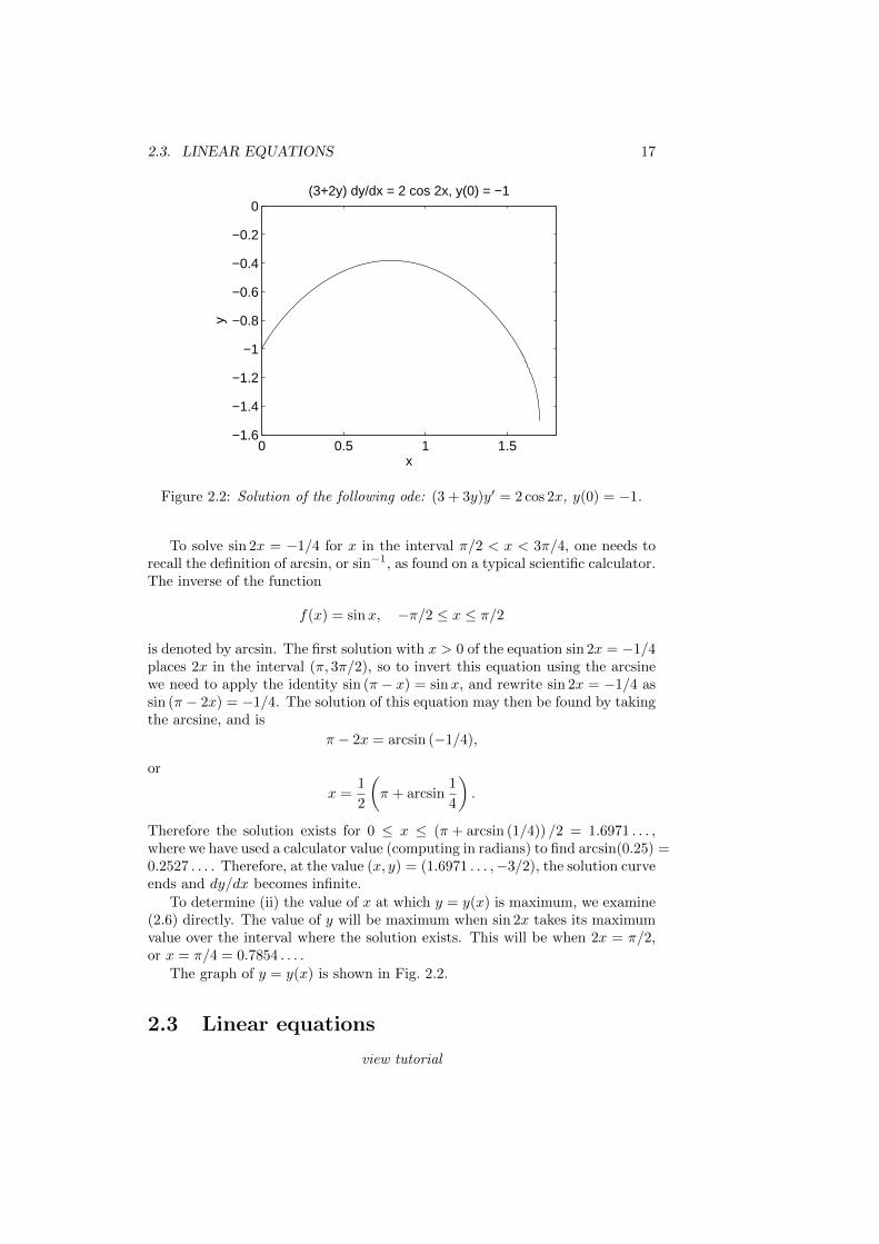
Example: Solve 𝑑𝑦𝑑𝑥 = 2 cos 2𝑥
3+2𝑦 , with 𝑦(0) = −1. (i) For what values of
𝑥 > 0 does the solution exist? (ii) For what value of 𝑥 > 0 is 𝑦(𝑥)maximum?
Notice that the solution of the ode may not exist when 𝑦 = −3/2, since 𝑑𝑦/𝑑𝑥 →∞. We separate variables and integrate from initial conditions:
(3 + 2𝑦)𝑑𝑦 = 2 cos 2𝑥 𝑑𝑥∫ 𝑦
−1
(3 + 2𝑦)𝑑𝑦 = 2
∫ 𝑥
0
cos 2𝑥 𝑑𝑥
3𝑦 + 𝑦2]𝑦−1
= sin 2𝑥]𝑥0
𝑦2 + 3𝑦 + 2− sin 2𝑥 = 0
𝑦± =1
2[−3±
√1 + 4 sin 2𝑥].
Solving the quadratic equation for 𝑦 has introduced a spurious solution thatdoes not satisfy the initial conditions. We test:
𝑦±(0) =1
2[−3± 1] =
{-1;-2.
Only the + root satisfies the initial condition, so that the unique solution to theode and initial condition is
𝑦 =1
2[−3 +
√1 + 4 sin 2𝑥]. (2.6)
To determine (i) the values of 𝑥 > 0 for which the solution exists, we require
1 + 4 sin 2𝑥 ≥ 0,
or
sin 2𝑥 ≥ −1
4. (2.7)
Notice that at 𝑥 = 0, we have sin 2𝑥 = 0; at 𝑥 = 𝜋/4, we have sin 2𝑥 = 1;at 𝑥 = 𝜋/2, we have sin 2𝑥 = 0; and at 𝑥 = 3𝜋/4, we have sin 2𝑥 = −1 Wetherefore need to determine the value of 𝑥 such that sin 2𝑥 = −1/4, with 𝑥 inthe range 𝜋/2 < 𝑥 < 3𝜋/4. The solution to the ode will then exist for all 𝑥between zero and this value.
2.3. LINEAR EQUATIONS 17
0 0.5 1 1.5−1.6
−1.4
−1.2
−1
−0.8
−0.6
−0.4
−0.2
0
x
y
(3+2y) dy/dx = 2 cos 2x, y(0) = −1
Figure 2.2: Solution of the following ode: (3 + 3𝑦)𝑦′ = 2 cos 2𝑥, 𝑦(0) = −1.
To solve sin 2𝑥 = −1/4 for 𝑥 in the interval 𝜋/2 < 𝑥 < 3𝜋/4, one needs torecall the definition of arcsin, or sin−1, as found on a typical scientific calculator.The inverse of the function
𝑓(𝑥) = sin𝑥, −𝜋/2 ≤ 𝑥 ≤ 𝜋/2
is denoted by arcsin. The first solution with 𝑥 > 0 of the equation sin 2𝑥 = −1/4places 2𝑥 in the interval (𝜋, 3𝜋/2), so to invert this equation using the arcsinewe need to apply the identity sin (𝜋 − 𝑥) = sin𝑥, and rewrite sin 2𝑥 = −1/4 assin (𝜋 − 2𝑥) = −1/4. The solution of this equation may then be found by takingthe arcsine, and is
𝜋 − 2𝑥 = arcsin (−1/4),
or
𝑥 =1
2
(𝜋 + arcsin
1
4
).
Therefore the solution exists for 0 ≤ 𝑥 ≤ (𝜋 + arcsin (1/4)) /2 = 1.6971 . . . ,where we have used a calculator value (computing in radians) to find arcsin(0.25) =0.2527 . . . . Therefore, at the value (𝑥, 𝑦) = (1.6971 . . . ,−3/2), the solution curveends and 𝑑𝑦/𝑑𝑥 becomes infinite.
To determine (ii) the value of 𝑥 at which 𝑦 = 𝑦(𝑥) is maximum, we examine(2.6) directly. The value of 𝑦 will be maximum when sin 2𝑥 takes its maximumvalue over the interval where the solution exists. This will be when 2𝑥 = 𝜋/2,or 𝑥 = 𝜋/4 = 0.7854 . . . .
The graph of 𝑦 = 𝑦(𝑥) is shown in Fig. 2.2.
2.3 Linear equations
view tutorial

18 CHAPTER 2. FIRST-ORDER ODES
The first-order linear differential equation (linear in 𝑦 and its derivative) can bewritten in the form
𝑑𝑦
𝑑𝑥+ 𝑝(𝑥)𝑦 = 𝑔(𝑥), (2.8)
with the initial condition 𝑦(𝑥0) = 𝑦0. Linear first-order equations can be inte-grated using an integrating factor 𝜇(𝑥). First, we multiply (2.8) by 𝜇(𝑥):
𝜇(𝑥)
[𝑑𝑦
𝑑𝑥+ 𝑝(𝑥)𝑦
]= 𝜇(𝑥)𝑔(𝑥). (2.9)
Next, we try to determine an integrating factor so that
𝜇(𝑥)
[𝑑𝑦
𝑑𝑥+ 𝑝(𝑥)𝑦
]=
𝑑
𝑑𝑥[𝜇(𝑥)𝑦], (2.10)
and (2.9) becomes𝑑
𝑑𝑥[𝜇(𝑥)𝑦] = 𝜇(𝑥)𝑔(𝑥). (2.11)
Equation (2.11) is easily integrated using 𝜇(𝑥0) = 𝜇0 and 𝑦(𝑥0) = 𝑦0:
𝜇(𝑥)𝑦 − 𝜇0𝑦0 =
∫ 𝑥
𝑥0
𝜇(𝑥)𝑔(𝑥)𝑑𝑥,
or
𝑦 =1
𝜇(𝑥)
(𝜇0𝑦0 +
∫ 𝑥
𝑥0
𝜇(𝑥)𝑔(𝑥)𝑑𝑥
). (2.12)
It remains to determine 𝜇(𝑥) from (2.10). Differentiating and expanding (2.10)yields
𝜇𝑑𝑦
𝑑𝑥+ 𝑝𝜇𝑦 =
𝑑𝜇
𝑑𝑥𝑦 + 𝜇
𝑑𝑦
𝑑𝑥;
and upon simplifying,𝑑𝜇
𝑑𝑥= 𝑝𝜇. (2.13)
Equation (2.13) is separable and can be integrated:∫ 𝜇
𝜇0
𝑑𝜇
𝜇=
∫ 𝑥
𝑥0
𝑝(𝑥)𝑑𝑥,
ln𝜇
𝜇0=
∫ 𝑥
𝑥0
𝑝(𝑥)𝑑𝑥,
𝜇(𝑥) = 𝜇0 exp
(∫ 𝑥
𝑥0
𝑝(𝑥)𝑑𝑥
).
Notice that since 𝜇0 cancels out of (2.12), it is customary to assign 𝜇0 = 1. Thesolution to (2.8) satisfying the initial condition 𝑦(𝑥0) = 𝑦0 is then traditionallywritten as
𝑦 =1
𝜇(𝑥)
(𝑦0 +
∫ 𝑥
𝑥0
𝜇(𝑥)𝑔(𝑥)𝑑𝑥
),
where
𝜇(𝑥) = exp
(∫ 𝑥
𝑥0
𝑝(𝑥)𝑑𝑥
).
This important result finds frequent use in applied mathematics.

2.3. LINEAR EQUATIONS 19
Example: Solve 𝑑𝑦𝑑𝑥 + 2𝑦 = 𝑒−𝑥, with 𝑦(0) = 3/4.
Note that this equation is not separable. With 𝑝(𝑥) = 2 and 𝑔(𝑥) = 𝑒−𝑥, wehave
𝜇(𝑥) = exp
(∫ 𝑥
0
2𝑑𝑥
)= 𝑒2𝑥,
and
𝑦 = 𝑒−2𝑥
(3
4+
∫ 𝑥
0
𝑒2𝑥𝑒−𝑥𝑑𝑥
)= 𝑒−2𝑥
(3
4+
∫ 𝑥
0
𝑒𝑥𝑑𝑥
)= 𝑒−2𝑥
(3
4+ (𝑒𝑥 − 1)
)= 𝑒−2𝑥
(𝑒𝑥 − 1
4
)= 𝑒−𝑥
(1− 1
4𝑒−𝑥
).
Example: Solve 𝑑𝑦𝑑𝑥 − 2𝑥𝑦 = 𝑥, with 𝑦(0) = 0.
This equation is separable, and we solve it in two ways. First, using an inte-grating factor with 𝑝(𝑥) = −2𝑥 and 𝑔(𝑥) = 𝑥:
𝜇(𝑥) = exp
(−2
∫ 𝑥
0
𝑥𝑑𝑥
)= 𝑒−𝑥2
,
and
𝑦 = 𝑒𝑥2
∫ 𝑥
0
𝑥𝑒−𝑥2
𝑑𝑥.
The integral can be done by substitution with 𝑢 = 𝑥2, 𝑑𝑢 = 2𝑥𝑑𝑥:∫ 𝑥
0
𝑥𝑒−𝑥2
𝑑𝑥 =1
2
∫ 𝑥2
0
𝑒−𝑢𝑑𝑢
= −1
2𝑒−𝑢
]𝑥2
0
=1
2
(1− 𝑒−𝑥2
).
Therefore,
𝑦 =1
2𝑒𝑥
2(1− 𝑒−𝑥2
)=
1
2
(𝑒𝑥
2
− 1).

20 CHAPTER 2. FIRST-ORDER ODES
Second, we integrate by separating variables:
𝑑𝑦
𝑑𝑥− 2𝑥𝑦 = 𝑥,
𝑑𝑦
𝑑𝑥= 𝑥(1 + 2𝑦),∫ 𝑦
0
𝑑𝑦
1 + 2𝑦=
∫ 𝑥
0
𝑥𝑑𝑥,
1
2ln (1 + 2𝑦) =
1
2𝑥2,
1 + 2𝑦 = 𝑒𝑥2
,
𝑦 =1
2
(𝑒𝑥
2
− 1).
The results from the two different solution methods are the same, and the choiceof method is a personal preference.
2.4 Applications
2.4.1 Compound interest with deposits or withdrawals
view tutorialThe equation for the growth of an investment with continuous compoundingof interest is a first-order differential equation. Let 𝑆(𝑡) be the value of theinvestment at time 𝑡, and let 𝑟 be the annual interest rate compounded afterevery time interval Δ𝑡. We can also include deposits (or withdrawals). Let 𝑘 bethe annual deposit amount, and suppose that an installment is deposited afterevery time interval Δ𝑡. The value of the investment at the time 𝑡+Δ𝑡 is thengiven by
𝑆(𝑡+Δ𝑡) = 𝑆(𝑡) + (𝑟Δ𝑡)𝑆(𝑡) + 𝑘Δ𝑡, (2.14)
where at the end of the time interval Δ𝑡, 𝑟Δ𝑡𝑆(𝑡) is the amount of interestcredited and 𝑘Δ𝑡 is the amount of money deposited (𝑘 > 0) or withdrawn(𝑘 < 0). As a numerical example, if the account held $10,000 at time 𝑡, and𝑟 = 6% per year and 𝑘 = $12,000 per year, say, and the compounding anddeposit period is Δ𝑡 = 1 month = 1/12 year, then the interest awarded afterone month is 𝑟Δ𝑡𝑆 = (0.06/12) × $10,000 = $50, and the amount deposited is𝑘Δ𝑡 = $1000.
Rearranging the terms of (2.14) to exhibit what will soon become a deriva-tive, we have
𝑆(𝑡+Δ𝑡)− 𝑆(𝑡)
Δ𝑡= 𝑟𝑆(𝑡) + 𝑘.
The equation for continuous compounding of interest and continuous depositsis obtained by taking the limit Δ𝑡 → 0. The resulting differential equation is
𝑑𝑆
𝑑𝑡= 𝑟𝑆 + 𝑘, (2.15)
which can solved with the initial condition 𝑆(0) = 𝑆0, where 𝑆0 is the initialcapital. We can solve either by separating variables or by using an integrating

2.4. APPLICATIONS 21
factor; I solve here by separating variables. Integrating from 𝑡 = 0 to a finaltime 𝑡, ∫ 𝑆
𝑆0
𝑑𝑆
𝑟𝑆 + 𝑘=
∫ 𝑡
0
𝑑𝑡,
1
𝑟ln
(𝑟𝑆 + 𝑘
𝑟𝑆0 + 𝑘
)= 𝑡,
𝑟𝑆 + 𝑘 = (𝑟𝑆0 + 𝑘)𝑒𝑟𝑡,
𝑆 =𝑟𝑆0𝑒
𝑟𝑡 + 𝑘𝑒𝑟𝑡 − 𝑘
𝑟,
𝑆 = 𝑆0𝑒𝑟𝑡 +
𝑘
𝑟𝑒𝑟𝑡(1− 𝑒−𝑟𝑡
), (2.16)
where the first term on the right-hand side of (2.16) comes from the initialinvested capital, and the second term comes from the deposits (or withdrawals).Evidently, compounding results in the exponential growth of an investment.
As a practical example, we can analyze a simple retirement plan. It iseasiest to assume that all amounts and returns are in real dollars (adjusted forinflation). Suppose a 25 year-old plans to set aside a fixed amount every year ofhis/her working life, invests at a real return of 6%, and retires at age 65. Howmuch must he/she invest each year to have $8,000,000 at retirement? We needto solve (2.16) for 𝑘 using 𝑡 = 40 years, 𝑆(𝑡) = $8,000,000, 𝑆0 = 0, and 𝑟 = 0.06per year. We have
𝑘 =𝑟𝑆(𝑡)
𝑒𝑟𝑡 − 1,
𝑘 =0.06× 8,000,000
𝑒0.06×40 − 1,
= $47,889 year−1.
To have saved approximately one million US$ at retirement, the worker wouldneed to save about HK$50,000 per year over his/her working life. Note that theamount saved over the worker’s life is approximately 40×$50,000 = $2,000,000,while the amount earned on the investment (at the assumed 6% real return) isapproximately $8,000,000− $2,000,000 = $6,000,000. The amount earned fromthe investment is about 3× the amount saved, even with the modest real returnof 6%. Sound investment planning is well worth the effort.
2.4.2 Chemical reactions
Suppose that two chemicals 𝐴 and 𝐵 react to form a product 𝐶, which we writeas
𝐴+𝐵𝑘→ 𝐶,
where 𝑘 is called the rate constant of the reaction. For simplicity, we will usethe same symbol 𝐶, say, to refer to both the chemical 𝐶 and its concentration.The law of mass action says that 𝑑𝐶/𝑑𝑡 is proportional to the product of theconcentrations 𝐴 and 𝐵, with proportionality constant 𝑘; that is,
𝑑𝐶
𝑑𝑡= 𝑘𝐴𝐵. (2.17)

22 CHAPTER 2. FIRST-ORDER ODES
Similarly, the law of mass action enables us to write equations for the time-derivatives of the reactant concentrations 𝐴 and 𝐵:
𝑑𝐴
𝑑𝑡= −𝑘𝐴𝐵,
𝑑𝐵
𝑑𝑡= −𝑘𝐴𝐵. (2.18)
The ode given by (2.17) can be solved analytically using conservation laws.From (2.17) and (2.18),
𝑑
𝑑𝑡(𝐴+ 𝐶) = 0 =⇒ 𝐴+ 𝐶 = 𝐴0,
𝑑
𝑑𝑡(𝐵 + 𝐶) = 0 =⇒ 𝐵 + 𝐶 = 𝐵0,
where 𝐴0 and 𝐵0 are the initial concentrations of the reactants, and we assumethat no product is initially present. Using the conservation laws, (2.17) becomes
𝑑𝐶
𝑑𝑡= 𝑘(𝐴0 − 𝐶)(𝐵0 − 𝐶), with 𝐶(0) = 0,
which is a nonlinear equation that may be integrated by separating variables.Separating and integrating, we obtain∫ 𝐶
0
𝑑𝐶
(𝐴0 − 𝐶)(𝐵0 − 𝐶)= 𝑘
∫ 𝑡
0
𝑑𝑡
= 𝑘𝑡. (2.19)
The remaining integral can be done using the method of partial fractions. Wewrite
1
(𝐴0 − 𝐶)(𝐵0 − 𝐶)=
𝑎
𝐴0 − 𝐶+
𝑏
𝐵0 − 𝐶. (2.20)
The cover-up method is the simplest method to determine the unknown coeffi-cients 𝑎 and 𝑏. To determine 𝑎, we multiply both sides of (2.20) by 𝐴0 −𝐶 andset 𝐶 = 𝐴0 to find
𝑎 =1
𝐵0 −𝐴0.
Similarly, to determine 𝑏, we multiply both sides of (2.20) by 𝐵0 − 𝐶 and set𝐶 = 𝐵0 to find
𝑏 =1
𝐴0 −𝐵0.
Therefore,
1
(𝐴0 − 𝐶)(𝐵0 − 𝐶)=
1
𝐵0 −𝐴0
(1
𝐴0 − 𝐶− 1
𝐵0 − 𝐶
),
and the remaining integral of (2.19) becomes (using 𝐶 < 𝐴0, 𝐵0)∫ 𝐶
0
𝑑𝐶
(𝐴0 − 𝐶)(𝐵0 − 𝐶)=
1
𝐵0 −𝐴0
(∫ 𝐶
0
𝑑𝐶
𝐴0 − 𝐶−∫ 𝐶
0
𝑑𝐶
𝐵0 − 𝐶
)
=1
𝐵0 −𝐴0
(− ln
(𝐴0 − 𝐶
𝐴0
)+ ln
(𝐵0 − 𝐶
𝐵0
))=
1
𝐵0 −𝐴0ln
(𝐴0(𝐵0 − 𝐶)
𝐵0(𝐴0 − 𝐶)
).
2.4. APPLICATIONS 23
Using this integral in (2.19), multiplying by (𝐵0 − 𝐴0) and exponentiating, weobtain
𝐴0(𝐵0 − 𝐶)
𝐵0(𝐴0 − 𝐶)= 𝑒(𝐵0−𝐴0)𝑘𝑡.
Solving for 𝐶, we finally obtain
𝐶(𝑡) = 𝐴0𝐵0𝑒(𝐵0−𝐴0)𝑘𝑡 − 1
𝐵0𝑒(𝐵0−𝐴0)𝑘𝑡 −𝐴0,
which appears to be a complicated expression, but has the simple limits
lim𝑡→∞
𝐶(𝑡) =
{𝐴0 if 𝐴0 < 𝐵0,
𝐵0 if 𝐵0 < 𝐴0,
= min(𝐴0, 𝐵0).
Hence, the reaction stops after one of the reactants is depleted; and the finalconcentration of product is equal to the initial concentration of the depletedreactant.
2.4.3 The terminal velocity of a falling mass
view tutorial
Using Newton’s law, we model a mass 𝑚 free falling under gravity but withair resistance. We assume that the force of air resistance is proportional to thespeed of the mass and opposes the direction of motion. We define the 𝑥-axis topoint in the upward direction, opposite the force of gravity. Near the surfaceof the Earth, the force of gravity is approximately constant and is given by−𝑚𝑔, with 𝑔 = 9.8m/s2 the usual gravitational acceleration. The force of airresistance is modeled by −𝑘𝑣, where 𝑣 is the vertical velocity of the mass and𝑘 is a positive constant. When the mass is falling, 𝑣 < 0 and the force of airresistance is positive, pointing upward and opposing the motion. The total forceon the mass is therefore given by 𝐹 = −𝑚𝑔−𝑘𝑣. With 𝐹 = 𝑚𝑎 and 𝑎 = 𝑑𝑣/𝑑𝑡,we obtain the differential equation
𝑚𝑑𝑣
𝑑𝑡= −𝑚𝑔 − 𝑘𝑣. (2.21)
The terminal velocity 𝑣∞ of the mass is defined as the asymptotic velocity afterair resistance balances the gravitational force. When the mass is at terminalvelocity, 𝑑𝑣/𝑑𝑡 = 0 so that
𝑣∞ = −𝑚𝑔
𝑘. (2.22)
The approach to the terminal velocity of a mass initially at rest is obtained bysolving (2.21) with initial condition 𝑣(0) = 0. The equation is both linear and

24 CHAPTER 2. FIRST-ORDER ODES
separable, and I solve by separating variables:
𝑚
∫ 𝑣
0
𝑑𝑣
𝑚𝑔 + 𝑘𝑣= −
∫ 𝑡
0
𝑑𝑡,
𝑚
𝑘ln
(𝑚𝑔 + 𝑘𝑣
𝑚𝑔
)= −𝑡,
1 +𝑘𝑣
𝑚𝑔= 𝑒−𝑘𝑡/𝑚,
𝑣 = −𝑚𝑔
𝑘
(1− 𝑒−𝑘𝑡/𝑚
).
Therefore, 𝑣 = 𝑣∞(1− 𝑒−𝑘𝑡/𝑚
), and 𝑣 approaches 𝑣∞ as the exponential term
decays to zero.As an example, a skydiver of mass 𝑚 = 100 kg with his parachute closed
may have a terminal velocity of 200 km/hr. With
𝑔 = (9.8m/s2)(10−3 km/m)(60 s/min)2(60min/hr)2 = 127, 008 km/hr
2,
one obtains from (2.22), 𝑘 = 63, 504 kg/hr. One-half of the terminal velocityfor free-fall (100 km/hr) is therefore attained when (1 − 𝑒−𝑘𝑡/𝑚) = 1/2, or 𝑡 =𝑚 ln 2/𝑘 ≈ 4 sec. Approximately 95% of the terminal velocity (190 km/hr ) isattained after 17 sec.
2.4.4 Escape velocity
view tutorialAn interesting physical problem is to find the smallest initial velocity for amass on the Earth’s surface to escape from the Earth’s gravitational field, theso-called escape velocity. Newton’s law of universal gravitation asserts that thegravitational force between two massive bodies is proportional to the product ofthe two masses and inversely proportional to the square of the distance betweenthem. For a mass 𝑚 a position 𝑥 above the surface of the Earth, the force onthe mass is given by
𝐹 = −𝐺𝑀𝑚
(𝑅+ 𝑥)2,
where 𝑀 and 𝑅 are the mass and radius of the Earth and 𝐺 is the gravitationalconstant. The minus sign occurs because the force on the mass 𝑚 points in theopposite direction of increasing 𝑥. The approximately constant acceleration 𝑔on the Earth’s surface corresponds to the absolute value of 𝐹/𝑚 when 𝑥 = 0:
𝑔 =𝐺𝑀
𝑅2,
and 𝑔 ≈ 9.8 m/s2. Newton’s law 𝐹 = 𝑚𝑎 for the mass 𝑚 is thus given by
𝑑2𝑥
𝑑𝑡2= − 𝐺𝑀
(𝑅+ 𝑥)2
= − 𝑔
(1 + 𝑥/𝑅)2. (2.23)
A useful trick allows us to solve this second-order differential equation asa first-order equation. First, note that 𝑑2𝑥/𝑑𝑡2 = 𝑑𝑣/𝑑𝑡. If we write 𝑣(𝑡) =

2.4. APPLICATIONS 25
𝑣(𝑥(𝑡))—considering the velocity of the mass 𝑚 to be a function of its distanceabove the Earth—we have using the chain rule
𝑑𝑣
𝑑𝑡=
𝑑𝑣
𝑑𝑥
𝑑𝑥
𝑑𝑡
= 𝑣𝑑𝑣
𝑑𝑥,
where we have used 𝑣 = 𝑑𝑥/𝑑𝑡. Therefore, (2.23) becomes the first-order ode
𝑣𝑑𝑣
𝑑𝑥= − 𝑔
(1 + 𝑥/𝑅)2,
which may be solved assuming an initial velocity 𝑣(𝑥 = 0) = 𝑣0 when the massis shot vertically from the Earth’s surface. Separating variables and integrating,we obtain ∫ 𝑣
𝑣0
𝑣𝑑𝑣 = −𝑔
∫ 𝑥
0
𝑑𝑥
(1 + 𝑥/𝑅)2.
The left integral is 12 (𝑣
2 − 𝑣20), and the right integral can be performed usingthe substitution 𝑢 = 1 + 𝑥/𝑅, 𝑑𝑢 = 𝑑𝑥/𝑅:∫ 𝑥
0
𝑑𝑥
(1 + 𝑥/𝑅)2= 𝑅
∫ 1+𝑥/𝑅
1
𝑑𝑢
𝑢2
= − 𝑅
𝑢
]1+𝑥/𝑅
1
= 𝑅− 𝑅2
𝑥+𝑅
=𝑅𝑥
𝑥+𝑅.
Therefore,1
2(𝑣2 − 𝑣20) = − 𝑔𝑅𝑥
𝑥+𝑅,
which when multiplied by 𝑚 is an expression of the conservation of energy (thechange of the kinetic energy of the mass is equal to the change in the potentialenergy). Solving for 𝑣2,
𝑣2 = 𝑣20 −2𝑔𝑅𝑥
𝑥+𝑅.
The escape velocity is defined as the minimum initial velocity 𝑣0 such thatthe mass can escape to infinity. Therefore, 𝑣0 = 𝑣escape when 𝑣 → 0 as 𝑥 → ∞.Taking this limit, we have
𝑣2escape = lim𝑥→∞
2𝑔𝑅𝑥
𝑥+𝑅
= 2𝑔𝑅.
With 𝑅 ≈ 6350 km and 𝑔 = 127, 008 km/hr2, we determine 𝑣escape =
√2𝑔𝑅 ≈
40 000 km/hr.

26 CHAPTER 2. FIRST-ORDER ODES
2.4.5 The logistic equation
Let 𝑁 = 𝑁(𝑡) be the size of a population at time 𝑡 and let 𝑟 be the growthrate. The Malthusian growth model (Thomas Malthus, 1766-1834), similar toa compound interest model, is given by
𝑑𝑁
𝑑𝑡= 𝑟𝑁.
Under a Malthusian growth model, a population grows exponentially like
𝑁(𝑡) = 𝑁0𝑒𝑟𝑡,
where 𝑁0 is the initial population size. However, when the population growthis constrained by limited resources, a heuristic modification to the Malthusiangrowth model results in the Verhulst equation,
𝑑𝑁
𝑑𝑡= 𝑟𝑁
(1− 𝑁
𝐾
), (2.24)
where 𝐾 is called the carrying capacity of the environment. Making (2.24)dimensionless using 𝜏 = 𝑟𝑡 and 𝑥 = 𝑁/𝐾 leads to the logistic equation,
𝑑𝑥
𝑑𝜏= 𝑥(1− 𝑥),
where we may assume the initial condition 𝑥(0) = 𝑥0 > 0. Separating variablesand integrating ∫ 𝑥
𝑥0
𝑑𝑥
𝑥(1− 𝑥)=
∫ 𝜏
0
𝑑𝜏.
The integral on the left-hand-side can be done using the method of partialfractions:
1
𝑥(1− 𝑥)=
𝑎
𝑥+
𝑏
1− 𝑥
=𝑎+ (𝑏− 𝑎)𝑥
𝑥(1− 𝑥);
and equating the coefficients of the numerators proportional to 𝑥0 and 𝑥1, wehave 𝑎 = 𝑏 = 1. Therefore,∫ 𝑥
𝑥0
𝑑𝑥
𝑥(1− 𝑥)=
∫ 𝑥
𝑥0
𝑑𝑥
𝑥+
∫ 𝑥
𝑥0
𝑑𝑥
(1− 𝑥)
= ln𝑥
𝑥0− ln
1− 𝑥
1− 𝑥0
= ln𝑥(1− 𝑥0)
𝑥0(1− 𝑥)
= 𝜏.

2.4. APPLICATIONS 27
Solving for 𝑥, we first exponentiate both sides and then isolate 𝑥:
𝑥(1− 𝑥0)
𝑥0(1− 𝑥)= 𝑒𝜏 ,
𝑥(1− 𝑥0) = 𝑥0𝑒𝜏 − 𝑥𝑥0𝑒
𝜏 ,
𝑥(1− 𝑥0 + 𝑥0𝑒𝜏 ) = 𝑥0𝑒
𝜏 ,
𝑥 =𝑥0
𝑥0 + (1− 𝑥0)𝑒−𝜏. (2.25)
We observe that for 𝑥0 > 0, we have lim𝜏→∞ 𝑥(𝜏) = 1, corresponding to
lim𝑡→∞
𝑁(𝑡) = 𝐾.
The population, therefore, grows in size until it reaches the carrying capacity ofits environment.

28 CHAPTER 2. FIRST-ORDER ODES

Chapter 3
Second-order lineardifferential equations withconstant coefficients
Reference: Boyce and DiPrima, Chapter 3
The general second-order linear differential equation with independent variable𝑡 and dependent variable 𝑥 = 𝑥(𝑡) is given by
��+ 𝑝(𝑡)��+ 𝑞(𝑡)𝑥 = 𝑔(𝑡), (3.1)
where we have used the standard physics notation �� = 𝑑𝑥/𝑑𝑡 and �� = 𝑑2𝑥/𝑑𝑡2.A unique solution of (3.1) requires initial values 𝑥(𝑡0) = 𝑥0 and ��(𝑡0) = 𝑢0.The equation with constant coefficients—on which we will devote considerableeffort—assumes that 𝑝(𝑡) and 𝑞(𝑡) are constants, independent of time. Thesecond-order linear ode is said to be homogeneous if 𝑔(𝑡) = 0.
3.1 The Euler method
view tutorialIn general, (3.1) can not be solved analytically, and we begin by deriving analgorithm for numerical solution. We write the second-order ode as a pair offirst-order odes by defining 𝑢 = ��, and writing the first-order system as
�� = 𝑢, (3.2)
�� = 𝑓(𝑡, 𝑥, 𝑢), (3.3)
where𝑓(𝑡, 𝑥, 𝑢) = −𝑝(𝑡)𝑢− 𝑞(𝑡)𝑥+ 𝑔(𝑡).
The first ode, (3.2), gives the slope of the tangent line to the curve 𝑥 = 𝑥(𝑡);the second ode, (3.3), gives the slope of the tangent line to the curve 𝑢 = 𝑢(𝑡).Beginning at the initial values (𝑥, 𝑢) = (𝑥0, 𝑢0) at the time 𝑡 = 𝑡0, we movealong the tangent lines to determine 𝑥1 = 𝑥(𝑡0 +Δ𝑡) and 𝑢1 = 𝑢(𝑡0 +Δ𝑡):
𝑥1 = 𝑥0 +Δ𝑡𝑢0,
𝑢1 = 𝑢0 +Δ𝑡𝑓(𝑡0, 𝑥0, 𝑢0).
29

30 CHAPTER 3. SECOND-ORDER ODES, CONSTANT COEFFICIENTS
The values 𝑥1 and 𝑢1 at the time 𝑡1 = 𝑡0+Δ𝑡 are then used as new initial valuesto march the solution forward to time 𝑡2 = 𝑡1 + Δ𝑡. As long as 𝑓(𝑡, 𝑥, 𝑢) is awell-behaved function, the numerical solution converges to the unique solutionof the ode as Δ𝑡 → 0.
3.2 The principle of superposition
view tutorialConsider the second-order linear homogeneous ode:
��+ 𝑝(𝑡)��+ 𝑞(𝑡)𝑥 = 0; (3.4)
and suppose that 𝑋1(𝑡) and 𝑋2(𝑡) are solutions to (3.4). We consider a linearcombination of 𝑋1 and 𝑋2 by letting
𝑋(𝑡) = 𝑐1𝑋1(𝑡) + 𝑐2𝑋2(𝑡), (3.5)
with 𝑐1 and 𝑐2 constants. The principle of superposition states that 𝑋(𝑡) is alsoa solution of (3.4). To prove this, we compute
�� + 𝑝�� + 𝑞𝑋 = 𝑐1��1 + 𝑐2��2 + 𝑝(𝑐1��1 + 𝑐2��2
)+ 𝑞 (𝑐1𝑋1 + 𝑐2𝑋2)
= 𝑐1
(��1 + 𝑝��1 + 𝑞𝑋1
)+ 𝑐2
(��2 + 𝑝��2 + 𝑞𝑋2
)= 𝑐1 × 0 + 𝑐2 × 0
= 0,
since 𝑋1 and 𝑋2 were assumed to be solutions of (3.4). We have therefore shownthat any linear combination of solutions to the second-order linear homogeneousode is also a solution.
3.3 The Wronskian
view tutorialSuppose that having determined 𝑋1(𝑡) and 𝑋2(𝑡), we attempt to write thegeneral solution to (3.4) as (3.5). We must then ask whether this general solutionwill be able to satisfy any two arbitrary initial conditions given by
𝑥(𝑡0) = 𝑥0, ��(𝑡0) = 𝑢0. (3.6)
Applying these initial conditions to (3.5), we obtain
𝑐1𝑋1(𝑡0) + 𝑐2𝑋2(𝑡0) = 𝑥0,
𝑐1��1(𝑡0) + 𝑐2��2(𝑡0) = 𝑢0, (3.7)
which is observed to be a system of two linear equations for the two unknowns𝑐1 and 𝑐2. Solution of (3.7) by standard methods results in
𝑐1 =𝑥0��2(𝑡0)− 𝑢0𝑋2(𝑡0)
𝑊, 𝑐2 =
𝑢0𝑋1(𝑡0)− 𝑥0��1(𝑡0)
𝑊,

3.4. HOMOGENEOUS ODES 31
where 𝑊 is called the Wronskian and is given by
𝑊 = 𝑋1(𝑡0)��2(𝑡0)− ��1(𝑡0)𝑋2(𝑡0). (3.8)
Evidently, the Wronskian must not be equal to zero (𝑊 = 0) for a solution toexist.
For examples, the two solutions
𝑋1(𝑡) = sin𝜔𝑡, 𝑋2(𝑡) = 𝐴 sin𝜔𝑡,
have a zero Wronskian at 𝑡 = 𝑡0, as can be shown by computing
𝑊 = (sin𝜔𝑡0) (𝐴𝜔 cos𝜔𝑡0)− (𝜔 cos𝜔𝑡0) (𝐴 sin𝜔𝑡0)
= 0;
while the two solutions
𝑋1(𝑡) = sin𝜔𝑡, 𝑋2(𝑡) = cos𝜔𝑡,
with 𝜔 = 0, have a nonzero Wronskian at 𝑡 = 𝑡0, as can be shown by computing
𝑊 = (sin𝜔𝑡0) (−𝜔 sin𝜔𝑡0)− (𝜔 cos𝜔𝑡0) (cos𝜔𝑡0)
= −𝜔.
When the Wronskian is not equal to zero, we say that the two solutions𝑋1(𝑡) and 𝑋2(𝑡) are linearly independent. The concept of linear independenceis borrowed from linear algebra, and indeed, the set of all functions that satisfy(3.4) can be shown to form a two-dimensional vector space.
3.4 Second-order linear homogeneous ode withconstant coefficients
view tutorialWe now study solutions of the homogeneous, constant coefficient ode, writtenas
𝑎��+ 𝑏��+ 𝑐𝑥 = 0, (3.9)
with 𝑎, 𝑏, and 𝑐 constants. Such an equation arises for the charge on a capacitorin an unpowered RLC electrical circuit, or for the position of a freely-oscillatingfrictional mass on a spring. Our solution method finds two linearly independentsolutions to (3.9), multiplies each of these solutions by a constant, and addsthem. The two free constants can then be used to satisfy whatever initialconditions are given.
Because of the differential properties of the exponential function, a naturalansatz, or guess, for the form of the solution to (3.9) is 𝑥 = 𝑒𝑟𝑡, where 𝑟 is aconstant to be determined. Successive differentiation results in �� = 𝑟𝑒𝑟𝑡 and�� = 𝑟2𝑒𝑟𝑡, and substitution into (3.9) yields
𝑎𝑟2𝑒𝑟𝑡 + 𝑏𝑟𝑒𝑟𝑡 + 𝑐𝑒𝑟𝑡 = 0. (3.10)
Our choice of exponential function is now rewarded by the explicit cancelationof 𝑒𝑟𝑡 in (3.10). The result is a quadratic equation for the unknown constant 𝑟:
𝑎𝑟2 + 𝑏𝑟 + 𝑐 = 0. (3.11)

32 CHAPTER 3. SECOND-ORDER ODES, CONSTANT COEFFICIENTS
Our ansatz has thus converted a differential equation into an algebraic equation.Equation (3.11) is called the characteristic equation of (3.9). Using the quadraticformula, the two solutions of the characteristic equation (3.11) are given by
𝑟± =1
2𝑎
(−𝑏±
√𝑏2 − 4𝑎𝑐
).
There are three cases to consider: (1) if 𝑏2 − 4𝑎𝑐 > 0, then the two roots aredistinct and real; (2) if 𝑏2−4𝑎𝑐 < 0, then the two roots are distinct and complexconjugates of each other; (3) if 𝑏2 − 4𝑎𝑐 = 0, then the two roots are degenerateand there is only one real root. We will consider these three cases in turn.
3.4.1 Real, distinct roots
When 𝑟+ = 𝑟− are real roots, then the general solution to (3.9) can be writtenas a linear superposition of the two solutions 𝑒𝑟+𝑡 and 𝑒𝑟−𝑡; that is,
𝑥(𝑡) = 𝑐1𝑒𝑟+𝑡 + 𝑐2𝑒
𝑟−𝑡.
The unknown constants 𝑐1 and 𝑐2 can then be determined by the initial condi-tions 𝑥(𝑡0) = 𝑥0 and ��(𝑡0) = 𝑢0. We now present two examples.
Example 1: Solve �� + 5�� + 6𝑥 = 0 with 𝑥(0) = 2, ��(0) = 3, and find themaximum value attained by 𝑥.
view tutorialWe take as our ansatz 𝑥 = 𝑒𝑟𝑡 and obtain the characteristic equation
𝑟2 + 5𝑟 + 6 = 0,
which factors to
(𝑟 + 3)(𝑟 + 2) = 0.
The general solution to the ode is thus
𝑥(𝑡) = 𝑐1𝑒−2𝑡 + 𝑐2𝑒
−3𝑡.
The solution for �� obtained by differentiation is
��(𝑡) = −2𝑐1𝑒−2𝑡 − 3𝑐2𝑒
−3𝑡.
Use of the initial conditions then results in two equations for the two unknownconstant 𝑐1 and 𝑐2:
𝑐1 + 𝑐2 = 2,
−2𝑐1 − 3𝑐2 = 3.
Adding three times the first equation to the second equation yields 𝑐1 = 9; andthe first equation then yields 𝑐2 = 2− 𝑐1 = −7. Therefore, the unique solutionthat satisfies both the ode and the initial conditions is
𝑥(𝑡) = 9𝑒−2𝑡 − 7𝑒−3𝑡.

3.4. HOMOGENEOUS ODES 33
Note that although both exponential terms decay in time, their sum increasesinitially since ��(0) > 0. The maximum value of 𝑥 occurs at the time 𝑡𝑚 when�� = 0, or
−18𝑒−2𝑡𝑚 + 21𝑒−3𝑡𝑚 = 0,
which may be solved for 𝑡𝑚:
𝑡𝑚 = ln
(7
6
).
The maximum 𝑥𝑚 = 𝑥(𝑡𝑚) is then determined to be
𝑥𝑚 = 9
(6
7
)2
− 7
(6
7
)3
=
(6
7
)2
(9− 6)
=108
49.
Example 2: Solve ��− 𝑥 = 0 with 𝑥(0) = 𝑥0, ��(0) = 𝑢0.
Again our ansatz is 𝑥 = 𝑒𝑟𝑡, and we obtain the characteristic equation
𝑟2 − 1 = 0,
with solution 𝑟± = ±1. Therefore, the general solution for 𝑥 is
𝑥(𝑡) = 𝑐1𝑒𝑡 + 𝑐2𝑒
−𝑡,
and the derivative satisfies
��(𝑡) = 𝑐1𝑒𝑡 − 𝑐2𝑒
−𝑡.
Initial conditions are satisfied when
𝑐1 + 𝑐2 = 𝑥0,
𝑐1 − 𝑐2 = 𝑢0.
Adding and subtracting these equations, we determine
𝑐1 =1
2(𝑥0 + 𝑢0) , 𝑐2 =
1
2(𝑥0 − 𝑢0) ,
so that after rearranging terms
𝑥(𝑡) = 𝑥0
(𝑒𝑡 + 𝑒−𝑡
2
)+ 𝑢0
(𝑒𝑡 − 𝑒−𝑡
2
).
The terms in parentheses are the usual definitions of the hyperbolic cosine andsine functions; that is,
cosh 𝑡 =𝑒𝑡 + 𝑒−𝑡
2, sinh 𝑡 =
𝑒𝑡 − 𝑒−𝑡
2.

34 CHAPTER 3. SECOND-ORDER ODES, CONSTANT COEFFICIENTS
Our solution can therefore be rewritten as
𝑥(𝑡) = 𝑥0 cosh 𝑡+ 𝑢0 sinh 𝑡.
Note that the relationships between the trigonometric functions and the complexexponentials were given by
cos 𝑡 =𝑒𝑖𝑡 + 𝑒−𝑖𝑡
2, sin 𝑡 =
𝑒𝑖𝑡 − 𝑒−𝑖𝑡
2𝑖,
so that
cosh 𝑡 = cos 𝑖𝑡, sinh 𝑡 = −𝑖 sin 𝑖𝑡.
Also note that the hyperbolic trigonometric functions satisfy the differentialequations
𝑑
𝑑𝑡sinh 𝑡 = cosh 𝑡,
𝑑
𝑑𝑡cosh 𝑡 = sinh 𝑡,
which though similar to the differential equations satisfied by the more com-monly used trigonometric functions, is absent a minus sign.
3.4.2 Complex conjugate, distinct roots
view tutorialWe now consider a characteristic equation (3.11) with 𝑏2−4𝑎𝑐 < 0, so the rootsoccur as complex conjugate pairs. With
𝜆 = − 𝑏
2𝑎, 𝜇 =
1
2𝑎
√4𝑎𝑐− 𝑏2,
the two roots of the characteristic equation are 𝜆 + 𝑖𝜇 and 𝜆 − 𝑖𝜇. We havethus found the following two complex exponential solutions to the differentialequation:
𝑍1 = 𝑒𝜆𝑡𝑒𝑖𝜇𝑡, 𝑍2 = 𝑒𝜆𝑡𝑒−𝑖𝜇𝑡.
Applying the principle of superposition, any linear combination of 𝑍1 and 𝑍2
is also a solution to the second-order ode, and we can form two different linearcombinations that are real. They are given by
𝑋1(𝑡) =𝑍1 + 𝑍2
2
= 𝑒𝜆𝑡(𝑒𝑖𝜇𝑡 + 𝑒−𝑖𝜇𝑡
2
)= 𝑒𝜆𝑡 cos𝜇𝑡,
and
𝑋2(𝑡) =𝑍1 − 𝑍2
2𝑖
= 𝑒𝜆𝑡(𝑒𝑖𝜇𝑡 − 𝑒−𝑖𝜇𝑡
2𝑖
)= 𝑒𝜆𝑡 sin𝜇𝑡.
3.4. HOMOGENEOUS ODES 35
Having found the two real solutions 𝑋1(𝑡) and 𝑋2(𝑡), we can then apply theprinciple of superposition again to determine the general solution 𝑥(𝑡) to be
𝑥(𝑡) = 𝑒𝜆𝑡 (𝐴 cos𝜇𝑡+𝐵 sin𝜇𝑡) . (3.12)
It is best to memorize this result. The real part of the roots of the characteristicequation goes into the exponential function; the imaginary part goes into theargument of cosine and sine.
Example 1: Solve ��+ 𝑥 = 0 with 𝑥(0) = 𝑥0 and ��(0) = 𝑢0.
view tutorial
The characteristic equation is
𝑟2 + 1 = 0,
with roots
𝑟± = ±𝑖.
The general solution of the ode is therefore
𝑥(𝑡) = 𝐴 cos 𝑡+𝐵 sin 𝑡.
The derivative is
��(𝑡) = −𝐴 sin 𝑡+𝐵 cos 𝑡.
Applying the initial conditions:
𝑥(0) = 𝐴 = 𝑥0, ��(0) = 𝐵 = 𝑢0;
so that the final solution is
𝑥(𝑡) = 𝑥0 cos 𝑡+ 𝑢0 sin 𝑡.
Recall that we wrote the analogous solution to the ode �� − 𝑥 = 0 as 𝑥(𝑡) =𝑥0 cosh 𝑡+ 𝑢0 sinh 𝑡.
Example 2: Solve ��+ ��+ 𝑥 = 0 with 𝑥(0) = 1 and ��(0) = 0.
The characteristic equation is
𝑟2 + 𝑟 + 1 = 0,
with roots
𝑟± = −1
2± 𝑖
√3
2.
The general solution of the ode is therefore
𝑥(𝑡) = 𝑒−12 𝑡
(𝐴 cos
√3
2𝑡+𝐵 sin
√3
2𝑡
).

36 CHAPTER 3. SECOND-ORDER ODES, CONSTANT COEFFICIENTS
The derivative is
��(𝑡) = −1
2𝑒−
12 𝑡
(𝐴 cos
√3
2𝑡+𝐵 sin
√3
2𝑡
)
+
√3
2𝑒−
12 𝑡
(−𝐴 sin
√3
2𝑡+𝐵 cos
√3
2𝑡
).
Applying the initial conditions 𝑥(0) = 1 and ��(0) = 0:
𝐴 = 1,
−1
2𝐴+
√3
2𝐵 = 0;
or
𝐴 = 1, 𝐵 =
√3
3.
Therefore,
𝑥(𝑡) = 𝑒−12 𝑡
(cos
√3
2𝑡+
√3
3sin
√3
2𝑡
).
3.4.3 Repeated roots
view tutorialFinally, we consider the characteristic equation,
𝑎𝑟2 + 𝑏𝑟 + 𝑐 = 0,
with 𝑏2 − 4𝑎𝑐 = 0. The degenerate root is then given by
𝑟 = − 𝑏
2𝑎,
yielding only a single solution to the ode:
𝑥1(𝑡) = exp
(− 𝑏𝑡
2𝑎
). (3.13)
To satisfy two initial conditions, a second independent solution must be found,and apparently this second solution is not of the form of our ansatz 𝑥 = exp (𝑟𝑡).
One method to determine this missing second solution is to try the ansatz
𝑥(𝑡) = 𝑦(𝑡)𝑥1(𝑡), (3.14)
where 𝑦(𝑡) is an unknown function that satisfies the differential equation ob-tained by substituting (3.14) into (3.9). This general technique is called thereduction of order method and enables one to find a second solution of a ho-mogeneous linear differential equation if one solution is known. If the originaldifferential equation is of order 𝑛, the differential equation for 𝑦 = 𝑦(𝑡) reducesto one of order 𝑛− 1.
Here, however, we will determine this missing second solution through alimiting process. We start with the solution obtained for complex roots of the

3.4. HOMOGENEOUS ODES 37
characteristic equation, and then arrive at the solution obtained for degenerateroots by taking the limit 𝜇 → 0.
Now, the general solution for complex roots was given by (3.12), and toproperly limit this solution as 𝜇 → 0 requires first satisfying the specific initialconditions 𝑥(0) = 𝑥0 and ��(0) = 𝑢0. Solving for 𝐴 and 𝐵, the general solutiongiven by (3.12) becomes the specific solution
𝑥(𝑡;𝜇) = 𝑒𝜆𝑡(𝑥0 cos𝜇𝑡+
𝑢0 − 𝜆𝑥0
𝜇sin𝜇𝑡
).
Here, we have written 𝑥 = 𝑥(𝑡;𝜇) to show explicitly that 𝑥 depends on 𝜇.
Taking the limit as 𝜇 → 0, and using lim𝜇→0 𝜇−1 sin𝜇𝑡 = 𝑡, we have
lim𝜇→0
𝑥(𝑡;𝜇) = 𝑒𝜆𝑡(𝑥0 + (𝑢0 − 𝜆𝑥0)𝑡
).
The second solution is observed to be a constant, 𝑢0 − 𝜆𝑥0, times 𝑡 times thefirst solution, 𝑒𝜆𝑡. Our general solution to the ode (3.9) when 𝑏2 − 4𝑎𝑐 = 0 cantherefore be written in the form
𝑥(𝑡) = (𝑐1 + 𝑐2𝑡)𝑒𝑟𝑡,
where 𝑟 is the repeated root of the characteristic equation. The main result tobe remembered is that for the case of repeated roots, the second solution is 𝑡times the first solution.
Example: Solve ��+ 2��+ 𝑥 = 0 with 𝑥(0) = 1 and ��(0) = 0.
The characteristic equation is
𝑟2 + 2𝑟 + 1 = (𝑟 + 1)2
= 0,
which has a repeated root given by 𝑟 = −1. Therefore, the general solution tothe ode is
𝑥(𝑡) = 𝑐1𝑒−𝑡 + 𝑐2𝑡𝑒
−𝑡,
with derivative
��(𝑡) = −𝑐1𝑒−𝑡 + 𝑐2𝑒
−𝑡 − 𝑐2𝑡𝑒−𝑡.
Applying the initial conditions:
𝑐1 = 1,
−𝑐1 + 𝑐2 = 0,
so that 𝑐1 = 𝑐2 = 1. Therefore, the solution is
𝑥(𝑡) = (1 + 𝑡)𝑒−𝑡.

38 CHAPTER 3. SECOND-ORDER ODES, CONSTANT COEFFICIENTS
3.5 Second-order linear inhomogeneous ode
We now consider the general second-order linear inhomogeneous ode (3.1):
��+ 𝑝(𝑡)��+ 𝑞(𝑡)𝑥 = 𝑔(𝑡), (3.15)
with initial conditions 𝑥(𝑡0) = 𝑥0 and ��(𝑡0) = 𝑢0. There is a three-step solutionmethod when the inhomogeneous term 𝑔(𝑡) = 0. (i) Find the general solutionof the homogeneous equation
��+ 𝑝(𝑡)��+ 𝑞(𝑡)𝑥 = 0. (3.16)
Let us denote the homogeneous solution by
𝑥ℎ(𝑡) = 𝑐1𝑋1(𝑡) + 𝑐2𝑋2(𝑡),
where 𝑋1 and 𝑋2 are linearly independent solutions of (3.16), and 𝑐1 and 𝑐2are as yet undetermined constants. (ii) Find any particular solution 𝑥𝑝 of theinhomogeneous equation (3.15). This particular solution can be found, for ex-ample, by the the method of undetermined coefficients discussed below, when𝑔(𝑡) is a combination of polynomials, exponentials, sines and cosines. (iii) Writethe general solution of (3.15) as the sum of the homogeneous and particularsolutions,
𝑥(𝑡) = 𝑥ℎ(𝑡) + 𝑥𝑝(𝑡), (3.17)
and apply the initial conditions to determine the constants 𝑐1 and 𝑐2. Note thatbecause of the linearity of (3.15),
��+ 𝑝��+ 𝑞𝑥 =𝑑2
𝑑𝑡2(𝑥ℎ + 𝑥𝑝) + 𝑝
𝑑
𝑑𝑡(𝑥ℎ + 𝑥𝑝) + 𝑞(𝑥ℎ + 𝑥𝑝)
= (��ℎ + 𝑝��ℎ + 𝑞𝑥ℎ) + (��𝑝 + 𝑝��𝑝 + 𝑞𝑥𝑝)
= 0 + 𝑔
= 𝑔,
so that (3.17) solves (3.15), and the two free constants in 𝑥ℎ can be used tosatisfy the initial conditions.
We will consider here only the constant coefficient case, and we now illustratethis solution method by an example.
Example: Solve ��− 3��− 4𝑥 = 3𝑒2𝑡 with 𝑥(0) = 1 and ��(0) = 0.
view tutorialFirst, we solve the homogeneous equation. The characteristic equation is
𝑟2 − 3𝑟 − 4 = (𝑟 − 4)(𝑟 + 1)
= 0,
so that𝑥ℎ(𝑡) = 𝑐1𝑒
4𝑡 + 𝑐2𝑒−𝑡.
Second, we find a particular solution of the inhomogeneous equation. The formof the particular solution is chosen such that the exponential will cancel out ofboth sides of the ode. The ansatz we choose is
𝑥(𝑡) = 𝐴𝑒2𝑡, (3.18)

3.5. INHOMOGENEOUS ODES 39
where 𝐴 is a yet undetermined coefficient. Upon substituting 𝑥 into the ode,differentiating using the chain rule, and canceling the exponential, we obtain
4𝐴− 6𝐴− 4𝐴 = 3,
from which we determine 𝐴 = −1/2. Obtaining a solution for 𝐴 independent of𝑡 justifies the ansatz (3.18). Third, we write the general solution to the ode asthe sum of the homogeneous and particular solutions, and determine 𝑐1 and 𝑐2that satisfy the initial conditions. We have
𝑥(𝑡) = 𝑐1𝑒4𝑡 + 𝑐2𝑒
−𝑡 − 1
2𝑒2𝑡;
and taking the derivative,
��(𝑡) = 4𝑐1𝑒4𝑡 − 𝑐2𝑒
−𝑡 − 𝑒2𝑡.
Applying the initial conditions,
𝑐1 + 𝑐2 −1
2= 1,
4𝑐1 − 𝑐2 − 1 = 0;
or
𝑐1 + 𝑐2 =3
2,
4𝑐1 − 𝑐2 = 1.
This system of linear equations can be solved for 𝑐1 by adding the equationsto obtain 𝑐1 = 1/2, after which 𝑐2 = 1 can be determined from the first equa-tion. Therefore, the solution for 𝑥(𝑡) that satisfies both the ode and the initialconditions is given by
𝑥(𝑡) =1
2𝑒4𝑡 − 1
2𝑒2𝑡 + 𝑒−𝑡
=1
2𝑒4𝑡(1− 𝑒−2𝑡 + 2𝑒−5𝑡
),
where we have grouped the terms in the solution to better display the asymptoticbehavior for large 𝑡.
We now find particular solutions for some relatively simple inhomogeneousterms using this method of undetermined coefficients.
Example: Find a particular solution of ��− 3��− 4𝑥 = 2 sin 𝑡.
view tutorialWe show two methods for finding a particular solution. The first more directmethod tries the ansatz
𝑥(𝑡) = 𝐴 cos 𝑡+𝐵 sin 𝑡,
where the argument of cosine and sine must agree with the argument of sine inthe inhomogeneous term. The cosine term is required because the derivative ofsine is cosine. Upon substitution into the differential equation, we obtain
(−𝐴 cos 𝑡−𝐵 sin 𝑡)− 3 (−𝐴 sin 𝑡+𝐵 cos 𝑡)− 4 (𝐴 cos 𝑡+𝐵 sin 𝑡) = 2 sin 𝑡,

40 CHAPTER 3. SECOND-ORDER ODES, CONSTANT COEFFICIENTS
or regrouping terms,
− (5𝐴+ 3𝐵) cos 𝑡+ (3𝐴− 5𝐵) sin 𝑡 = 2 sin 𝑡.
This equation is valid for all 𝑡, and in particular for 𝑡 = 0 and 𝜋/2, for whichthe sine and cosine functions vanish. For these two values of 𝑡, we find
5𝐴+ 3𝐵 = 0, 3𝐴− 5𝐵 = 2;
and solving for 𝐴 and 𝐵, we obtain
𝐴 =3
17, 𝐵 = − 5
17.
The particular solution is therefore given by
𝑥𝑝 =1
17(3 cos 𝑡− 5 sin 𝑡) .
The second solution method makes use of the relation 𝑒𝑖𝑡 = cos 𝑡+ 𝑖 sin 𝑡 toconvert the sine inhomogeneous term to an exponential function. We introducethe complex function 𝑧(𝑡) by letting
𝑧(𝑡) = 𝑥(𝑡) + 𝑖𝑦(𝑡),
and rewrite the differential equation in complex form. We can rewrite the equa-tion in one of two ways. On the one hand, if we use sin 𝑡 = Re{−𝑖𝑒𝑖𝑡}, then thedifferential equation is written as
𝑧 − 3�� − 4𝑧 = −2𝑖𝑒𝑖𝑡; (3.19)
and by equating the real and imaginary parts, this equation becomes the tworeal differential equations
��− 3��− 4𝑥 = 2 sin 𝑡, 𝑦 − 3�� − 4𝑦 = −2 cos 𝑡.
The solution we are looking for, then, is 𝑥𝑝(𝑡) = Re{𝑧𝑝(𝑡)}.On the other hand, if we write sin 𝑡 = Im{𝑒𝑖𝑡}, then the complex differential
equation becomes𝑧 − 3�� − 4𝑧 = 2𝑒𝑖𝑡, (3.20)
which becomes the two real differential equations
��− 3��− 4𝑥 = 2 cos 𝑡, 𝑦 − 3�� − 4𝑦 = 2 sin 𝑡.
Here, the solution we are looking for is 𝑥𝑝(𝑡) = Im{𝑧𝑝(𝑡)}.We will proceed here by solving (3.20). We now have an exponential as the
inhomogeneous term, and we can make the ansatz
𝑧(𝑡) = 𝐶𝑒𝑖𝑡,
where we now expect 𝐶 to be a complex constant. Upon substitution into theode (3.19) and using 𝑖2 = −1:
−𝐶 − 3𝑖𝐶 − 4𝐶 = 2;

3.6. FIRST-ORDER LINEAR INHOMOGENEOUS ODES REVISITED 41
or solving for 𝐶:
𝐶 =−2
5 + 3𝑖
=−2(5− 3𝑖)
(5 + 3𝑖)(5− 3𝑖)
=−10 + 6𝑖
34
=−5 + 3𝑖
17.
Therefore,
𝑥𝑝 = Im{𝑧𝑝}
= Im
{1
17(−5 + 3𝑖)(cos 𝑡+ 𝑖 sin 𝑡)
}=
1
17(3 cos 𝑡− 5 sin 𝑡).
Example: Find a particular solution of ��+ ��− 2𝑥 = 𝑡2.
view tutorialThe correct ansatz here is the polynomial
𝑥(𝑡) = 𝐴𝑡2 +𝐵𝑡+ 𝐶.
Upon substitution into the ode
2𝐴+ 2𝐴𝑡+𝐵 − 2𝐴𝑡2 − 2𝐵𝑡− 2𝐶 = 𝑡2,
or−2𝐴𝑡2 + 2(𝐴−𝐵)𝑡+ (2𝐴+𝐵 − 2𝐶)𝑡0 = 𝑡2.
Equating powers of 𝑡,
−2𝐴 = 1, 2(𝐴−𝐵) = 0, 2𝐴+𝐵 − 2𝐶 = 0;
and solving,
𝐴 = −1
2, 𝐵 = −1
2, 𝐶 = −3
4.
The particular solution is therefore
𝑥𝑝(𝑡) = −1
2𝑡2 − 1
2𝑡− 3
4.
3.6 First-order linear inhomogeneous odes re-visited
The first-order linear ode can be solved by use of an integrating factor. Here Ishow that odes having constant coefficients can be solved by our newly learnedsolution method.

42 CHAPTER 3. SECOND-ORDER ODES, CONSTANT COEFFICIENTS
Example: Solve ��+ 2𝑥 = 𝑒−𝑡 with 𝑥(0) = 3/4.
Rather than using an integrating factor, we follow the three-step approach: (i)find the general homogeneous solution; (ii) find a particular solution; (iii) addthem and satisfy initial conditions. Accordingly, we try the ansatz 𝑥ℎ(𝑡) = 𝑒𝑟𝑡
for the homogeneous ode ��+ 2𝑥 = 0 and find
𝑟 + 2 = 0, or 𝑟 = −2.
To find a particular solution, we try the ansatz 𝑥𝑝(𝑡) = 𝐴𝑒−𝑡, and upon substi-tution
−𝐴+ 2𝐴 = 1, or 𝐴 = 1.
Therefore, the general solution to the ode is
𝑥(𝑡) = 𝑐𝑒−2𝑡 + 𝑒−𝑡.
The single initial condition determines the unknown constant 𝑐:
𝑥(0) =3
4= 𝑐+ 1,
so that 𝑐 = −1/4. Hence,
𝑥(𝑡) = 𝑒−𝑡 − 1
4𝑒−2𝑡
= 𝑒−𝑡
(1− 1
4𝑒−𝑡
).
3.7 Resonance
view tutorialResonance occurs when the frequency of the inhomogeneous term matches thefrequency of the homogeneous solution. To illustrate resonance in its simplestembodiment, we consider the second-order linear inhomogeneous ode
��+ 𝜔20𝑥 = 𝑓 cos𝜔𝑡, 𝑥(0) = 𝑥0, ��(0) = 𝑢0. (3.21)
Our main goal is to determine what happens to the solution in the limit 𝜔 → 𝜔0.The homogeneous equation has characteristic equation
𝑟2 + 𝜔20 = 0,
so that 𝑟± = ±𝑖𝜔0. Therefore,
𝑥ℎ(𝑡) = 𝑐1 cos𝜔0𝑡+ 𝑐2 sin𝜔0𝑡. (3.22)
To find a particular solution, we note the absence of a first-derivative term,and simply try
𝑥(𝑡) = 𝐴 cos𝜔𝑡.
Upon substitution into the ode, we obtain
−𝜔2𝐴+ 𝜔20𝐴 = 𝑓,

3.7. RESONANCE 43
or
𝐴 =𝑓
𝜔20 − 𝜔2
.
Therefore,
𝑥𝑝(𝑡) =𝑓
𝜔20 − 𝜔2
cos𝜔𝑡.
Our general solution is thus
𝑥(𝑡) = 𝑐1 cos𝜔0𝑡+ 𝑐2 sin𝜔0𝑡+𝑓
𝜔20 − 𝜔2
cos𝜔𝑡,
with derivative
��(𝑡) = 𝜔0(𝑐2 cos𝜔0𝑡− 𝑐1 sin𝜔0𝑡)−𝑓𝜔
𝜔20 − 𝜔2
sin𝜔𝑡.
Initial conditions are satisfied when
𝑥0 = 𝑐1 +𝑓
𝜔20 − 𝜔2
,
𝑢0 = 𝑐2𝜔0,
so that
𝑐1 = 𝑥0 −𝑓
𝜔20 − 𝜔2
, 𝑐2 =𝑢0
𝜔0.
Therefore, the solution to the ode that satisfies the initial conditions is
𝑥(𝑡) =
(𝑥0 −
𝑓
𝜔20 − 𝜔2
)cos𝜔0𝑡+
𝑢0
𝜔0sin𝜔0𝑡+
𝑓
𝜔20 − 𝜔2
cos𝜔𝑡
= 𝑥0 cos𝜔0𝑡+𝑢0
𝜔0sin𝜔0𝑡+
𝑓(cos𝜔𝑡− cos𝜔0𝑡)
𝜔20 − 𝜔2
,
where we have grouped together terms proportional to the forcing amplitude 𝑓 .Resonance occurs in the limit 𝜔 → 𝜔0; that is, the frequency of the inhomo-
geneous term (the external force) matches the frequency of the homogeneoussolution (the free oscillation). By L’Hospital’s rule, the limit of the term pro-portional to 𝑓 is found by differentiating with respect to 𝜔:
lim𝜔→𝜔0
𝑓(cos𝜔𝑡− cos𝜔0𝑡)
𝜔20 − 𝜔2
= lim𝜔→𝜔0
−𝑓𝑡 sin𝜔𝑡
−2𝜔
=𝑓𝑡 sin𝜔0𝑡
2𝜔0.
(3.23)
At resonance, the term proportional to the amplitude 𝑓 of the inhomogeneousterm increases linearly with 𝑡, resulting in larger-and-larger amplitudes of oscil-lation for 𝑥(𝑡). In general, if the inhomogeneous term in the differential equationis a solution of the corresponding homogeneous differential equation, then thecorrect ansatz for the particular solution is a constant times the inhomogeneousterm times 𝑡.
To illustrate this same example further, we return to the original ode, nowassumed to be exactly at resonance,
��+ 𝜔20𝑥 = 𝑓 cos𝜔0𝑡,

44 CHAPTER 3. SECOND-ORDER ODES, CONSTANT COEFFICIENTS
and find a particular solution directly. The particular solution is the real partof the particular solution of
𝑧 + 𝜔20𝑧 = 𝑓𝑒𝑖𝜔0𝑡,
and because the inhomogeneous term is a solution of the corresponding homo-geneous equation, we take as our ansatz
𝑧𝑝 = 𝐴𝑡𝑒𝑖𝜔0𝑡.
We have��𝑝 = 𝐴𝑒𝑖𝜔0𝑡 (1 + 𝑖𝜔0𝑡) , 𝑧𝑝 = 𝐴𝑒𝑖𝜔0𝑡
(2𝑖𝜔0 − 𝜔2
0𝑡);
and upon substitution into the ode
𝑧𝑝 + 𝜔20𝑧𝑝 = 𝐴𝑒𝑖𝜔0𝑡
(2𝑖𝜔0 − 𝜔2
0𝑡)+ 𝜔2
0𝐴𝑡𝑒𝑖𝜔0𝑡
= 2𝑖𝜔0𝐴𝑒𝑖𝜔0𝑡
= 𝑓𝑒𝑖𝜔0𝑡.
Therefore,
𝐴 =𝑓
2𝑖𝜔0,
and
𝑥𝑝 = Re{ 𝑓𝑡
2𝑖𝜔0𝑒𝑖𝜔0𝑡}
=𝑓𝑡 sin𝜔0𝑡
2𝜔0,
the same result as (3.23).
Example: Find a particular solution of ��− 3��− 4𝑥 = 5𝑒−𝑡 .
view tutorialIf we naively try the ansatz
𝑥 = 𝐴𝑒−𝑡,
and substitute this into the inhomogeneous differential equation, we obtain
𝐴+ 3𝐴− 4𝐴 = 5,
or 0 = 5, which is clearly nonsense. Our ansatz therefore fails to find a solution.The cause of this failure is that the corresponding homogeneous equation hassolution
𝑥ℎ = 𝑐1𝑒4𝑡 + 𝑐2𝑒
−𝑡,
so that the inhomogeneous term 5𝑒−𝑡 is one of the solutions of the homogeneousequation. To find a particular solution, we should therefore take as our ansatz
𝑥 = 𝐴𝑡𝑒−𝑡,
with first- and second-derivatives given by
�� = 𝐴𝑒−𝑡(1− 𝑡), �� = 𝐴𝑒−𝑡(−2 + 𝑡).

3.8. DAMPED RESONANCE 45
Substitution into the differential equation yields
𝐴𝑒−𝑡(−2 + 𝑡)− 3𝐴𝑒−𝑡(1− 𝑡)− 4𝐴𝑡𝑒−𝑡 = 5𝑒−𝑡.
The terms containing 𝑡 cancel out of this equation, resulting in −5𝐴 = 5, or𝐴 = −1. Therefore, the particular solution is
𝑥𝑝 = −𝑡𝑒−𝑡.
3.8 Damped resonance
view tutorialA more realistic study of resonance assumes an additional damping term. Theforced, damped harmonic oscillator equation may be written as
𝑚��+ 𝛾��+ 𝑘𝑥 = 𝐹 cos𝜔𝑡, (3.24)
where 𝑚 > 0 is the oscillator’s mass, 𝛾 > 0 is the damping coefficient, 𝑘 >0 is the spring constant, and 𝐹 is the amplitude of the external force. Thehomogeneous equation has characteristic equation
𝑚𝑟2 + 𝛾𝑟 + 𝑘 = 0,
so that
𝑟± = − 𝛾
2𝑚± 1
2𝑚
√𝛾2 − 4𝑚𝑘.
When 𝛾2 − 4𝑚𝑘 < 0, the motion of the unforced oscillator is said to be under-damped; when 𝛾2 − 4𝑚𝑘 > 0, overdamped, and; when 𝛾2 − 4𝑚𝑘 = 0, criticallydamped. For all all three types of damping, the roots of the characteristic equa-tion satisfy Re(𝑟±) < 0. Therefore, both linearly independent homogeneoussolutions decay exponentially to zero, and the long-time asymptotic solutionof (3.24) reduces to the (non-decaying) particular solution. Since the initialconditions are satisfied by the free constants multiplying the (decaying) homo-geneous solutions, the long-time asymptotic solution is independent of the initialconditions.
If we are only interested in the long-time asymptotic solution of (3.24), wecan proceed directly to the determination of a particular solution. As before,we consider the complex ode
𝑚𝑧 + 𝛾�� + 𝑘𝑧 = 𝐹𝑒𝑖𝜔𝑡,
with 𝑥𝑝 = Re(𝑧𝑝). With the ansatz 𝑧𝑝 = 𝐴𝑒𝑖𝜔𝑡, we have
−𝑚𝜔2𝐴+ 𝑖𝛾𝜔𝐴+ 𝑘𝐴 = 𝐹,
or
𝐴 =𝐹
(𝑘 −𝑚𝜔2) + 𝑖𝛾𝜔.
To simplify, we define 𝜔0 =√𝑘/𝑚, which corresponds to the natural frequency
of the undamped oscillator, and define Γ = 𝛾𝜔/𝑚 and 𝑓 = 𝐹/𝑚. Therefore,
𝐴 =𝑓
(𝜔20 − 𝜔2) + 𝑖Γ
=
(𝑓
(𝜔20 − 𝜔2)2 + Γ2
)((𝜔2
0 − 𝜔2)− 𝑖Γ).
(3.25)

46 CHAPTER 3. SECOND-ORDER ODES, CONSTANT COEFFICIENTS
To determine 𝑥𝑝, we utilize the polar form of a complex number. The complexnumber 𝑧 = 𝑥+ 𝑖𝑦 can be written in polar form as 𝑧 = 𝑟𝑒𝑖𝜑, where 𝑥 = 𝑟 cos𝜑,𝑦 = 𝑟 sin𝜑, and 𝑟 =
√𝑥2 + 𝑦2, tan𝜑 = 𝑦/𝑥. We therefore write
(𝜔20 − 𝜔2)− 𝑖Γ = 𝑟𝑒𝑖𝜑,
with
𝑟 =√(𝜔2
0 − 𝜔2)2 + Γ2, tan𝜑 =Γ
(𝜔2 − 𝜔20).
Using the polar form, 𝐴 in (3.25) becomes
𝐴 =
(𝑓√
(𝜔20 − 𝜔2)2 + Γ2
)𝑒𝑖𝜑,
and 𝑥𝑝 = Re(𝐴𝑒𝑖𝜔𝑡) becomes
𝑥𝑝 =
(𝑓√
(𝜔20 − 𝜔2)2 + Γ2
)Re(𝑒𝑖(𝜔𝑡+𝜑)
)=
(𝑓√
(𝜔20 − 𝜔2)2 + Γ2
)cos (𝜔𝑡+ 𝜑).
The particular solution given by (3.26), with 𝜔20 = 𝑘/𝑚, Γ = 𝛾𝜔/𝑚, 𝑓 = 𝐹/𝑚,
and tan𝜑 = 𝛾𝜔/𝑚(𝜔2 −𝜔20), is the long-time asymptotic solution of the forced,
damped, harmonic oscillator equation (3.24).We conclude with a couple of observations about (3.26). First, if the forcing
frequency 𝜔 is equal to the natural frequency 𝜔0 of the undamped oscillator, then𝐴 = −𝑖𝐹/𝛾𝜔0, and 𝑥𝑝 = (𝐹/𝛾𝜔0) sin𝜔0𝑡. The oscillator position is observedto be 𝜋/2 out of phase with the external force, or in other words, the velocityof the oscillator, not the position, is in phase with the force. Second, the valueof the forcing frequency 𝜔𝑚 that maximizes the amplitude of oscillation is thevalue of 𝜔 that minimizes the denominator of (3.26). To determine 𝜔𝑚 we thusminimize the function 𝑔(𝜔2) with respect to 𝜔2, where
𝑔(𝜔2) = (𝜔20 − 𝜔2)2 +
𝛾2𝜔2
𝑚2.
Taking the derivative of 𝑔 with respect to 𝜔2 and setting this to zero to determine𝜔𝑚 yields
2(𝜔2𝑚 − 𝜔2
0) +𝛾2
𝑚2= 0,
or
𝜔2𝑚 = 𝜔2
0 −𝛾2
2𝑚2.
We can interpret this result by saying that damping lowers the “resonance”frequency of the undamped oscillator.

Chapter 4
The Laplace transformReference: Boyce and DiPrima, Chapter 6
The Laplace transform is most useful for solving linear, constant-coefficientode’s when the inhomogeneous term or its derivative is discontinuous. Althoughode’s with discontinuous inhomogeneous terms can also be solved by adoptingalready learned methods, we will see that the Laplace transform technique pro-vides a simpler, more elegant solution.
4.1 Definitions and properties of the forwardand inverse Laplace transforms
view tutorialThe main idea is to Laplace transform the constant-coefficient differential equa-tion for 𝑥(𝑡) into a simpler algebraic equation for the Laplace-transformed func-tion 𝑋(𝑠), solve this algebraic equation, and then transform 𝑋(𝑠) back into𝑥(𝑡). The correct definition of the Laplace transform and the properties thatthis transform satisfies makes this solution method possible.
An exponential ansatz is used in solving homogeneous constant-coefficientodes, and the exponential function correspondingly plays a key role in definingthe Laplace transform. The Laplace transform of 𝑓(𝑡), denoted by 𝐹 (𝑠) =ℒ{𝑓(𝑡)}, is defined by the integral transform
𝐹 (𝑠) =
∫ ∞
0
𝑒−𝑠𝑡𝑓(𝑡)𝑑𝑡. (4.1)
The improper integral given by (4.1) diverges if 𝑓(𝑡) grows faster than 𝑒𝑠𝑡 forlarge 𝑡. Accordingly, some restriction on the range of 𝑠 may be required toguarantee convergence of (4.1), and we will assume without further elaborationthat these restrictions are always satisfied.
One of the useful properties of the Laplace transform is that it is linear. Wehave
ℒ{𝑐1𝑓1(𝑡) + 𝑐2𝑓2(𝑡)} =
∫ ∞
0
𝑒−𝑠𝑡(𝑐1𝑓1(𝑡) + 𝑐2𝑓2(𝑡)
)𝑑𝑡
= 𝑐1
∫ ∞
0
𝑒−𝑠𝑡𝑓1(𝑡)𝑑𝑡+ 𝑐2
∫ ∞
0
𝑒−𝑠𝑡𝑓2(𝑡)𝑑𝑡
= 𝑐1ℒ{𝑓1(𝑡)}+ 𝑐2ℒ{𝑓2(𝑡)}.
47

48 CHAPTER 4. THE LAPLACE TRANSFORM
𝑓(𝑡) = ℒ−1{𝐹 (𝑠)} 𝐹 (𝑠) = ℒ{𝑓(𝑡)}
1. 𝑒𝑎𝑡𝑓(𝑡) 𝐹 (𝑠− 𝑎)
2. 11
𝑠
3. 𝑒𝑎𝑡1
𝑠− 𝑎
4. 𝑡𝑛𝑛!
𝑠𝑛+1
5. 𝑡𝑛𝑒𝑎𝑡𝑛!
(𝑠− 𝑎)𝑛+1
6. sin 𝑏𝑡𝑏
𝑠2 + 𝑏2
7. cos 𝑏𝑡𝑠
𝑠2 + 𝑏2
8. 𝑒𝑎𝑡 sin 𝑏𝑡𝑏
(𝑠− 𝑎)2 + 𝑏2
9. 𝑒𝑎𝑡 cos 𝑏𝑡𝑠− 𝑎
(𝑠− 𝑎)2 + 𝑏2
10. 𝑡 sin 𝑏𝑡2𝑏𝑠
(𝑠2 + 𝑏2)2
11. 𝑡 cos 𝑏𝑡𝑠2 − 𝑏2
(𝑠2 + 𝑏2)2
12. 𝑢𝑐(𝑡)𝑒−𝑐𝑠
𝑠
13. 𝑢𝑐(𝑡)𝑓(𝑡− 𝑐) 𝑒−𝑐𝑠𝐹 (𝑠)
14. 𝛿(𝑡− 𝑐) 𝑒−𝑐𝑠
15. ��(𝑡) 𝑠𝑋(𝑠)− 𝑥(0)
16. ��(𝑡) 𝑠2𝑋(𝑠)− 𝑠𝑥(0)− ��(0)
Table 4.1: Table of Laplace Transforms
4.1. DEFINITION AND PROPERTIES 49
Another useful property of the Laplace transformation is that there is a one-to-one correspondence between functions and their Laplace transforms, so thatthe inverse Laplace transform (also linear) is well defined. This suggests thatconstruction of a table of Laplace transforms of commonly occurring functionsmay be useful in finding both Laplace and inverse Laplace transforms. Sucha table is shown in Table 4.1 (and this table will be distributed with the finalexam). In Table 4.1, 𝑛 is a positive integer. Also, the cryptic entries for 𝑢𝑐(𝑡)and 𝛿(𝑡− 𝑐) will be explained later in S4.3.
The rows of Table 4.1 can be determined by a combination of direct inte-gration and some tricks. We first compute directly the Laplace transform of𝑒𝑎𝑡𝑓(𝑡) (line 1):
ℒ{𝑒𝑎𝑡𝑓(𝑡)} =
∫ ∞
0
𝑒−𝑠𝑡𝑒𝑎𝑡𝑓(𝑡)𝑑𝑡
=
∫ ∞
0
𝑒−(𝑠−𝑎)𝑡𝑓(𝑡)𝑑𝑡
= 𝐹 (𝑠− 𝑎).
We also compute directly the Laplace transform of 1 (line 2):
ℒ{1} =
∫ ∞
0
𝑒−𝑠𝑡𝑑𝑡
= −1
𝑠𝑒−𝑠𝑡
]∞0
=1
𝑠.
Now, the Laplace transform of 𝑒𝑎𝑡 (line 3) may be found using these two results:
ℒ{𝑒𝑎𝑡} = ℒ{𝑒𝑎𝑡 · 1}
=1
𝑠− 𝑎.
(4.2)
The transform of 𝑡𝑛 (line 4) can be found by successive integration by parts. Amore interesting method uses Taylor series expansions for 𝑒𝑎𝑡 and 1/(𝑠−𝑎). Wehave
ℒ{𝑒𝑎𝑡} = ℒ
{ ∞∑𝑛=0
(𝑎𝑡)𝑛
𝑛!
}
=
∞∑𝑛=0
𝑎𝑛
𝑛!ℒ{𝑡𝑛}.
(4.3)
Also, with 𝑠 > 𝑎,
1
𝑠− 𝑎=
1
𝑠(1− 𝑎𝑠 )
=1
𝑠
∞∑𝑛=0
(𝑎𝑠
)𝑛=
∞∑𝑛=0
𝑎𝑛
𝑠𝑛+1.
(4.4)

50 CHAPTER 4. THE LAPLACE TRANSFORM
Using (4.2), and equating the coefficients of powers of 𝑎 in (4.3) and (4.4), resultsin line 4:
ℒ{𝑡𝑛} =𝑛!
𝑠𝑛+1.
The Laplace transform of 𝑡𝑛𝑒𝑎𝑡 (line 5) can be found from line 1 and line 4:
ℒ{𝑡𝑛𝑒𝑎𝑡} =𝑛!
(𝑠− 𝑎)𝑛+1.
The Laplace transform of sin 𝑏𝑡 (line 6) may be found from the Laplace transformof 𝑒𝑎𝑡 (line 3) using 𝑎 = 𝑖𝑏:
ℒ{sin 𝑏𝑡} = Im{ℒ{𝑒𝑖𝑏𝑡}
}= Im
{1
𝑠− 𝑖𝑏
}= Im
{𝑠+ 𝑖𝑏
𝑠2 + 𝑏2
}=
𝑏
𝑠2 + 𝑏2.
Similarly, the Laplace transform of cos 𝑏𝑡 (line 7) is
ℒ{cos 𝑏𝑡} = Re{ℒ{𝑒𝑖𝑏𝑡}
}=
𝑠
𝑠2 + 𝑏2.
The transform of 𝑒𝑎𝑡 sin 𝑏𝑡 (line 8) can be found from the transform of sin 𝑏𝑡(line 6) and line 1:
ℒ{𝑒𝑎𝑡 sin 𝑏𝑡} =𝑏
(𝑠− 𝑎)2 + 𝑏2;
and similarly for the transform of 𝑒𝑎𝑡 cos 𝑏𝑡:
ℒ{𝑒𝑎𝑡 cos 𝑏𝑡} =𝑠− 𝑎
(𝑠− 𝑎)2 + 𝑏2.
The Laplace transform of 𝑡 sin 𝑏𝑡 (line 10) can be found from the Laplace trans-form of 𝑡𝑒𝑎𝑡 (line 5 with 𝑛 = 1) using 𝑎 = 𝑖𝑏:
ℒ{𝑡 sin 𝑏𝑡} = Im{ℒ{𝑡𝑒𝑖𝑏𝑡}
}= Im
{1
(𝑠− 𝑖𝑏)2
}= Im
{(𝑠+ 𝑖𝑏)2
(𝑠2 + 𝑏2)2
}=
2𝑏𝑠
(𝑠2 + 𝑏2)2.
Similarly, the Laplace transform of 𝑡 cos 𝑏𝑡 (line 11) is
ℒ{𝑡 cos 𝑏𝑡} = Re{ℒ{𝑡𝑒𝑖𝑏𝑡}
}= Re
{(𝑠+ 𝑖𝑏)2
(𝑠2 + 𝑏2)2
}=
𝑠2 − 𝑏2
(𝑠2 + 𝑏2)2.

4.2. SOLUTION OF INITIAL VALUE PROBLEMS 51
We now transform the inhomogeneous constant-coefficient, second-order, lin-ear inhomogeneous ode for 𝑥 = 𝑥(𝑡),
𝑎��+ 𝑏��+ 𝑐𝑥 = 𝑔(𝑡),
making use of the linearity of the Laplace transform:
𝑎ℒ{��}+ 𝑏ℒ{��}+ 𝑐ℒ{𝑥} = ℒ{𝑔}.
To determine the Laplace transform of ��(𝑡) (line 15) in terms of the Laplacetransform of 𝑥(𝑡) and the initial conditions 𝑥(0) and ��(0), we define 𝑋(𝑠) =ℒ{𝑥(𝑡)}, and integrate ∫ ∞
0
𝑒−𝑠𝑡��𝑑𝑡
by parts. We let
𝑢 = 𝑒−𝑠𝑡 𝑑𝑣 = ��𝑑𝑡
𝑑𝑢 = −𝑠𝑒−𝑠𝑡𝑑𝑡 𝑣 = 𝑥.
Therefore, ∫ ∞
0
𝑒−𝑠𝑡��𝑑𝑡 = 𝑥𝑒−𝑠𝑡]∞0
+ 𝑠
∫ ∞
0
𝑒−𝑠𝑡𝑥𝑑𝑡
= 𝑠𝑋(𝑠)− 𝑥(0),
where assumed convergence of the Laplace transform requires
lim𝑡→∞
𝑥(𝑡)𝑒−𝑠𝑡 = 0.
Similarly, the Laplace transform of ��(𝑡) (line 16) is determined by integrating∫ ∞
0
𝑒−𝑠𝑡��𝑑𝑡
by parts and using the just derived result for the first derivative. We let
𝑢 = 𝑒−𝑠𝑡 𝑑𝑣 = ��𝑑𝑡
𝑑𝑢 = −𝑠𝑒−𝑠𝑡𝑑𝑡 𝑣 = ��,
so that ∫ ∞
0
𝑒−𝑠𝑡��𝑑𝑡 = ��𝑒−𝑠𝑡]∞0
+ 𝑠
∫ ∞
0
𝑒−𝑠𝑡��𝑑𝑡
= −��(0) + 𝑠(𝑠𝑋(𝑠)− 𝑥(0)
)= 𝑠2𝑋(𝑠)− 𝑠𝑥(0)− ��(0),
where similarly we assume lim𝑡→∞ ��(𝑡)𝑒−𝑠𝑡 = 0.
4.2 Solution of initial value problems
We begin with a simple homogeneous ode and show that the Laplace transformmethod yields an identical result to our previously learned method. We thenapply the Laplace transform method to solve an inhomogeneous equation.

52 CHAPTER 4. THE LAPLACE TRANSFORM
Example: Solve ��−��−2𝑥 = 0 with 𝑥(0) = 1 and ��(0) = 0 by two differentmethods.
view tutorial
The characteristic equation of the ode is determined from the ansatz 𝑥 = 𝑒𝑟𝑡
and is
𝑟2 − 𝑟 − 2 = (𝑟 − 2)(𝑟 + 1) = 0.
The general solution of the ode is therefore
𝑥(𝑡) = 𝑐1𝑒2𝑡 + 𝑐2𝑒
−𝑡.
To satisfy the initial conditions, we must have 1 = 𝑐1 + 𝑐2 and 0 = 2𝑐1 − 𝑐2,requiring 𝑐1 = 1
3 and 𝑐2 = 23 . Therefore, the solution to the ode that satisfies
the initial conditions is given by
𝑥(𝑡) =1
3𝑒2𝑡 +
2
3𝑒−𝑡. (4.5)
We now solve this example using the Laplace transform. Taking the Laplacetransform of both sides of the ode, using the linearity of the transform, andapplying our result for the transform of the first and second derivatives, we find
[𝑠2𝑋(𝑠)− 𝑠𝑥(0)− ��(0)]− [𝑠𝑋(𝑠)− 𝑥(0)]− [2𝑋(𝑠)] = 0,
or
𝑋(𝑠) =(𝑠− 1)𝑥(0) + ��(0)
𝑠2 − 𝑠− 2.
Note that the denominator of the right-hand-side is just the quadratic from thecharacteristic equation of the homogeneous ode, and that this factor arises fromthe derivatives of the exponential term in the Laplace transform integral.
Applying the initial conditions, we find
𝑋(𝑠) =𝑠− 1
(𝑠− 2)(𝑠+ 1). (4.6)
We have thus determined the Laplace transformed solution 𝑋(𝑠) = ℒ{𝑥(𝑡)}.We now need to compute the inverse Laplace transform 𝑥(𝑡) = ℒ−1{𝑋(𝑠)}.
However, direct inversion of (4.6) by searching Table 4.1 is not possible, buta partial fraction expansion may be useful. In particular, we write
𝑠− 1
(𝑠− 2)(𝑠+ 1)=
𝑎
𝑠− 2+
𝑏
𝑠+ 1. (4.7)
The cover-up method can be used to solve for 𝑎 and 𝑏. We multiply both sidesof (4.7) by 𝑠− 2 and put 𝑠 = 2 to isolate 𝑎:
𝑎 =𝑠− 1
𝑠+ 1
]𝑠=2
=1
3.
4.2. SOLUTION OF INITIAL VALUE PROBLEMS 53
Similarly, we multiply both sides of (4.7) by 𝑠+ 1 and put 𝑠 = −1 to isolate 𝑏:
𝑏 =𝑠− 1
𝑠− 2
]𝑠=−1
=2
3.
Therefore,
𝑋(𝑠) =1
3· 1
𝑠− 2+
2
3· 1
𝑠+ 1,
and line 3 of Table 4.1 gives us the inverse transforms of each term separatelyto yield
𝑥(𝑡) =1
3𝑒2𝑡 +
2
3𝑒−𝑡,
identical to (4.5).
Example: Solve �� + 𝑥 = sin 2𝑡 with 𝑥(0) = 2 and ��(0) = 1 by Laplacetransform methods.
Taking the Laplace transform of both sides of the ode, we find
𝑠2𝑋(𝑠)− 𝑠𝑥(0)− ��(0) +𝑋(𝑠) = ℒ{sin 2𝑡}
=2
𝑠2 + 4,
where the Laplace transform of sin 2𝑡 made use of line 6 of Table 4.1. Substi-tuting for 𝑥(0) and ��(0) and solving for 𝑋(𝑠), we obtain
𝑋(𝑠) =2𝑠+ 1
𝑠2 + 1+
2
(𝑠2 + 1)(𝑠2 + 4).
To determine the inverse Laplace transform from Table 4.1, we perform a partialfraction expansion of the second term:
2
(𝑠2 + 1)(𝑠2 + 4)=
𝑎𝑠+ 𝑏
𝑠2 + 1+
𝑐𝑠+ 𝑑
𝑠2 + 4. (4.8)
By inspection, we can observe that 𝑎 = 𝑐 = 0 and that 𝑑 = −𝑏. A quickcalculation shows that 3𝑏 = 2, or 𝑏 = 2/3. Therefore,
𝑋(𝑠) =2𝑠+ 1
𝑠2 + 1+
2/3
𝑠2 + 1− 2/3
(𝑠2 + 4)
=2𝑠
𝑠2 + 1+
5/3
𝑠2 + 1− 2/3
(𝑠2 + 4).
From lines 6 and 7 of Table 4.1, we obtain the solution by taking inverse Laplacetransforms of the three terms separately, where 𝑏 = 1 in the first two terms, and𝑏 = 2 in the third term:
𝑥(𝑡) = 2 cos 𝑡+5
3sin 𝑡− 1
3sin 2𝑡.

54 CHAPTER 4. THE LAPLACE TRANSFORM
4.3 Heaviside and Dirac delta functions
The Laplace transform technique becomes truly useful when solving odes withdiscontinuous or impulsive inhomogeneous terms, these terms commonly mod-eled using Heaviside or Dirac delta functions. We will discuss these functionsin turn, as well as their Laplace transforms.
4.3.1 Heaviside function
view tutorial
The Heaviside or unit step function, denoted here by 𝑢𝑐(𝑡), is zero for 𝑡 < 𝑐 andis one for 𝑡 ≥ 𝑐; that is,
𝑢𝑐(𝑡) =
{0, 𝑡 < 𝑐;1, 𝑡 ≥ 𝑐.
(4.9)
The precise value of 𝑢𝑐(𝑡) at the single point 𝑡 = 𝑐 is typically inconsequential.
The Heaviside function can be viewed as the step-up function. The step-down function—one for 𝑡 < 𝑐 and zero for 𝑡 ≥ 𝑐—is defined as
1− 𝑢𝑐(𝑡) =
{1, 𝑡 < 𝑐;0, 𝑡 ≥ 𝑐.
(4.10)
The step-up, step-down function—zero for 𝑡 < 𝑎, one for 𝑎 ≤ 𝑡 < 𝑏, and zerofor 𝑡 ≥ 𝑏—is defined as
𝑢𝑎(𝑡)− 𝑢𝑏(𝑡) =
⎧⎨⎩ 0, 𝑡 < 𝑎;1, 𝑎 ≤ 𝑡 < 𝑏;0, 𝑡 ≥ 𝑏.
(4.11)
The Laplace transform of the Heaviside function is determined by integra-tion:
ℒ{𝑢𝑐(𝑡)} =
∫ ∞
0
𝑒−𝑠𝑡𝑢𝑐(𝑡)𝑑𝑡
=
∫ ∞
𝑐
𝑒−𝑠𝑡𝑑𝑡
=𝑒−𝑐𝑠
𝑠,
and is given in line 12 of Table 4.1.
The Heaviside function can be used to represent a translation of a function𝑓(𝑡) a distance 𝑐 in the positive 𝑡 direction. We have
𝑢𝑐(𝑡)𝑓(𝑡− 𝑐) =
{0, 𝑡 < 𝑐;
f(t-c), 𝑡 ≥ 𝑐.
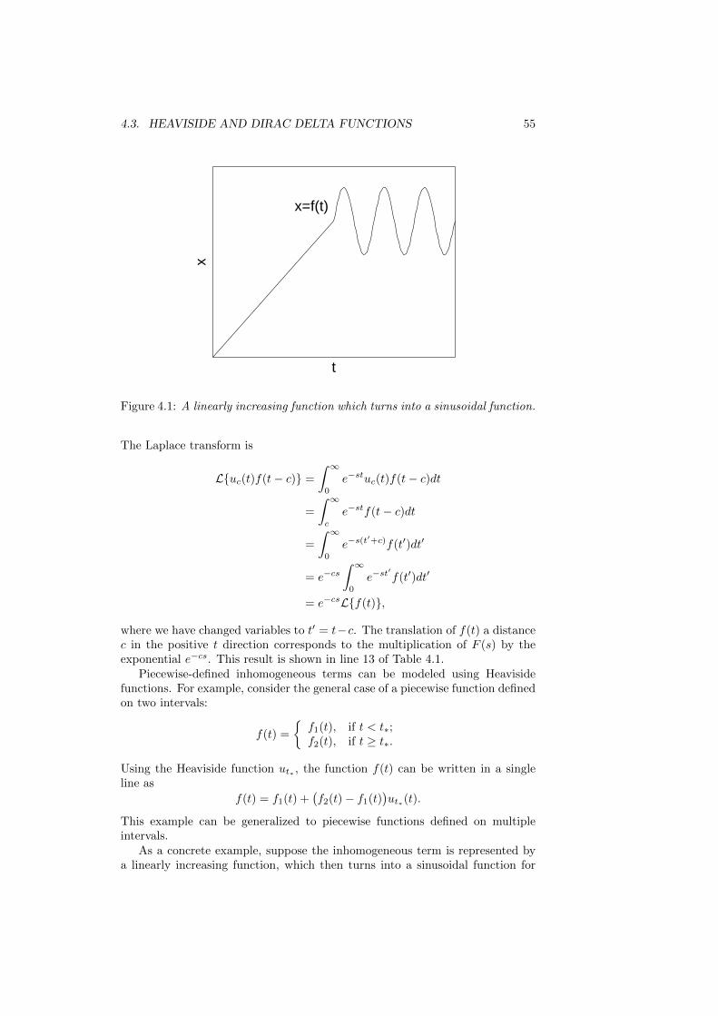
4.3. HEAVISIDE AND DIRAC DELTA FUNCTIONS 55
t
xx=f(t)
Figure 4.1: A linearly increasing function which turns into a sinusoidal function.
The Laplace transform is
ℒ{𝑢𝑐(𝑡)𝑓(𝑡− 𝑐)} =
∫ ∞
0
𝑒−𝑠𝑡𝑢𝑐(𝑡)𝑓(𝑡− 𝑐)𝑑𝑡
=
∫ ∞
𝑐
𝑒−𝑠𝑡𝑓(𝑡− 𝑐)𝑑𝑡
=
∫ ∞
0
𝑒−𝑠(𝑡′+𝑐)𝑓(𝑡′)𝑑𝑡′
= 𝑒−𝑐𝑠
∫ ∞
0
𝑒−𝑠𝑡′𝑓(𝑡′)𝑑𝑡′
= 𝑒−𝑐𝑠ℒ{𝑓(𝑡)},
where we have changed variables to 𝑡′ = 𝑡−𝑐. The translation of 𝑓(𝑡) a distance𝑐 in the positive 𝑡 direction corresponds to the multiplication of 𝐹 (𝑠) by theexponential 𝑒−𝑐𝑠. This result is shown in line 13 of Table 4.1.
Piecewise-defined inhomogeneous terms can be modeled using Heavisidefunctions. For example, consider the general case of a piecewise function definedon two intervals:
𝑓(𝑡) =
{𝑓1(𝑡), if 𝑡 < 𝑡*;𝑓2(𝑡), if 𝑡 ≥ 𝑡*.
Using the Heaviside function 𝑢𝑡* , the function 𝑓(𝑡) can be written in a singleline as
𝑓(𝑡) = 𝑓1(𝑡) +(𝑓2(𝑡)− 𝑓1(𝑡)
)𝑢𝑡*(𝑡).
This example can be generalized to piecewise functions defined on multipleintervals.
As a concrete example, suppose the inhomogeneous term is represented bya linearly increasing function, which then turns into a sinusoidal function for

56 CHAPTER 4. THE LAPLACE TRANSFORM
𝑡 > 𝑡*, as sketched in Fig. 4.1. Explicitly,
𝑓(𝑡) =
{𝑎𝑡, if 𝑡 < 𝑡*;𝑎𝑡* + 𝑏 sin
(𝜔(𝑡− 𝑡*)
), if 𝑡 ≥ 𝑡*.
We can rewrite 𝑓(𝑡) using the Heaviside function 𝑢𝑡*(𝑡):
𝑓(𝑡) = 𝑎𝑡+
(𝑏 sin
(𝜔(𝑡− 𝑡*)
)− 𝑎(𝑡− 𝑡*)
)· 𝑢𝑡*(𝑡).
This specific form of 𝑓(𝑡) enables a relatively easy Laplace transform. We canwrite
𝑓(𝑡) = 𝑎𝑡+ ℎ(𝑡− 𝑡*)𝑢𝑡*(𝑡),
where we have defined
ℎ(𝑡) = 𝑏 sin𝜔𝑡− 𝑎𝑡.
Using line 13, the Laplace transform of 𝑓(𝑡) is
𝐹 (𝑠) = 𝑎ℒ{𝑡}+ ℒ{ℎ(𝑡− 𝑡*)𝑢𝑡*(𝑡)}= 𝑎ℒ{𝑡}+ 𝑒−𝑡*𝑠ℒ{ℎ(𝑡)},
and where using lines 4 and 6,
ℒ{𝑡} =1
𝑠2, ℒ{ℎ(𝑡)} =
𝑏𝜔
𝑠2 + 𝜔2− 𝑎
𝑠2.
4.3.2 Dirac delta function
view tutorialThe Dirac delta function, denoted as 𝛿(𝑡), is defined by requiring that for anyfunction 𝑓(𝑡), ∫ ∞
−∞𝑓(𝑡)𝛿(𝑡)𝑑𝑡 = 𝑓(0).
The usual view of the shifted Dirac delta function 𝛿(𝑡 − 𝑐) is that it is zeroeverywhere except at 𝑡 = 𝑐, at which point it is infinite, and it integratesto unity. The Dirac delta function is technically not a function, but is whatmathematicians call a distribution. Nevertheless, in most cases of practicalinterest, it can be treated like a function, where physical results are obtainedfollowing a final integration.
There are many ways to represent the Dirac delta function as a limit of awell-defined function. For our purposes, the most useful representation makesuse of the step-up, step-down function of (4.11):
𝛿(𝑡− 𝑐) = lim𝜖→0
1
2𝜖(𝑢𝑐−𝜖(𝑡)− 𝑢𝑐+𝜖(𝑡)).
Before taking the limit, the well-defined step-up, step-down function is zeroexcept over a small interval of width 2𝜖 centered at 𝑡 = 𝑐, over which it takesthe large value 1/2𝜖. The integral of this function is one, independent of thevalue of 𝜖.

4.4. DISCONTINUOUS OR IMPULSIVE TERMS 57
The Laplace transform of the Dirac delta function is easily found by inte-gration using the definition of the delta function:
ℒ{𝛿(𝑡− 𝑐)} =
∫ ∞
0
𝑒−𝑠𝑡𝛿(𝑡− 𝑐)𝑑𝑡
= 𝑒−𝑐𝑠.
This result is shown in line 14 of Table 4.1.
4.4 Discontinuous or impulsive inhomogeneousterms
We now solve some more challenging ode’s with discontinuous or impulsiveinhomogeneous terms.
Example: Solve 2��+ ��+ 2𝑥 = 𝑢5(𝑡)− 𝑢20(𝑡), with 𝑥(0) = ��(0) = 0
The inhomogeneous term here is a step-up, step-down function that is unityover the interval (5, 20) and zero elsewhere. Taking the Laplace transform ofthe ode using Table 4.1,
2(𝑠2𝑋(𝑠)− 𝑠𝑥(0)− ��(0)
)+ 𝑠𝑋(𝑠)− 𝑥(0) + 2𝑋(𝑠) =
𝑒−5𝑠
𝑠− 𝑒−20𝑠
𝑠.
Using the initial values and solving for 𝑋(𝑠), we find
𝑋(𝑠) =𝑒−5𝑠 − 𝑒−20𝑠
𝑠(2𝑠2 + 𝑠+ 2).
To determine the solution for 𝑥(𝑡) we now need to find the inverse Laplacetransform. The exponential functions can be dealt with using line 13 of Table4.1. We write
𝑋(𝑠) = (𝑒−5𝑠 − 𝑒−20𝑠)𝐻(𝑠),
where
𝐻(𝑠) =1
𝑠(2𝑠2 + 𝑠+ 2).
Then using line 13, we have
𝑥(𝑡) = 𝑢5(𝑡)ℎ(𝑡− 5)− 𝑢20(𝑡)ℎ(𝑡− 20), (4.12)
where ℎ(𝑡) = ℒ−1{𝐻(𝑠)}.To determine ℎ(𝑡) we need the partial fraction expansion of 𝐻(𝑠). Since the
discriminant of 2𝑠2 + 𝑠+ 2 is negative, we have
1
𝑠(2𝑠2 + 𝑠+ 2)=
𝑎
𝑠+
𝑏𝑠+ 𝑐
2𝑠2 + 𝑠+ 2,
yielding the equation
1 = 𝑎(2𝑠2 + 𝑠+ 2) + (𝑏𝑠+ 𝑐)𝑠;
58 CHAPTER 4. THE LAPLACE TRANSFORM
or after equating powers of 𝑠,
2𝑎+ 𝑏 = 0, 𝑎+ 𝑐 = 0, 2𝑎 = 1,
yielding 𝑎 = 12 , 𝑏 = −1, and 𝑐 = − 1
2 . Therefore,
𝐻(𝑠) =1/2
𝑠−
𝑠+ 12
2𝑠2 + 𝑠+ 2.
Inspecting Table 4.1, the first term can be transformed using line 2, and thesecond term can be transformed using lines 8 and 9, provided we complete thesquare of the denominator and then massage the numerator. That is, first wecomplete the square:
2𝑠2 + 𝑠+ 2 = 2
(𝑠2 +
1
2𝑠+ 1
)= 2
((𝑠+
1
4)2 +
15
16
);
and next we write
𝑠+ 12
2𝑠2 + 𝑠+ 2=
𝑠+ 12
2((𝑠+ 1
4 )2 + 15
16
)=
(1
2
) (𝑠+ 14
)+ 1√
15
√1516
(𝑠+ 14 )
2 + 1516
.
Therefore, the function 𝐻(𝑠) can be written as
𝐻(𝑠) =
(1
2
)1
𝑠−(1
2
) (𝑠+ 1
4
)(𝑠+ 1
4 )2 + 15
16
−(
1
2√15
) √1516
(𝑠+ 14 )
2 + 1516
.
The first term is transformed using line 2, the second term using line 9 and thethird term using line 8. We finally obtain
ℎ(𝑡) =1
2− 1
2𝑒−𝑡/4 cos (
√15𝑡/4)−
(1
2√15
)𝑒−𝑡/4 sin (
√15𝑡/4)
=1
2
(1− 𝑒−𝑡/4
(cos (
√15𝑡/4)− 1√
15sin (
√15𝑡/4)
)), (4.13)
which when combined with (4.12) yields the rather complicated solution for𝑥(𝑡).
We briefly comment that it is also possible to solve this example withoutusing the Laplace transform. The key idea is that both 𝑥 and �� are continuousfunctions of 𝑡. Clearly from the form of the inhomogeneous term and the initialconditions, 𝑥(𝑡) = 0 for 0 ≤ 𝑡 ≤ 5. We then solve the ode between 5 ≤ 𝑡 ≤ 20with the inhomogeneous term equal to unity and initial conditions 𝑥(5) = ��(5) =0. This requires first finding the general homogeneous solution, next finding aparticular solution, and then adding the homogeneous and particular solutionsand solving for the two unknown constants. To simplify the algebra, note thatthe best ansatz to use to find the homogeneous solution is 𝑒𝑟(𝑡−5), and not 𝑒𝑟𝑡.

4.4. DISCONTINUOUS OR IMPULSIVE TERMS 59
Finally, we solve the homogeneous ode for 𝑡 ≥ 20 using as boundary conditionsthe previously determined values 𝑥(20) and ��(20), where we have made use ofthe continuity of 𝑥 and ��. The student may benefit by trying this as an exerciseand attempting to obtain a final solution that agrees with the form given by(4.12) and (4.13).
Example: Solve 2��+ ��+ 2𝑥 = 𝛿(𝑡− 5) with 𝑥(0) = ��(0) = 0
Here the inhomogeneous term is an impulse at time 𝑡 = 5. Taking the Laplacetransform of the ode using Table 4.1, and applying the initial conditions,
(2𝑠2 + 𝑠+ 2)𝑋(𝑠) = 𝑒−5𝑠,
so that
𝑋(𝑠) =𝑒−5𝑠
2𝑠2 + 𝑠+ 2
=1
2𝑒−5𝑠
(1
𝑠2 + 12𝑠+ 1
)=
1
2𝑒−5𝑠
(1
(𝑠+ 14 )
2 + 1516
)
=1
2
√16
15𝑒−5𝑠
⎛⎝√
1516
(𝑠+ 14 )
2 + 1516
⎞⎠ .
The inverse Laplace transform may now be computed using lines 8 and 13 ofTable 4.1:
𝑥(𝑡) =2√15
𝑢5(𝑡)𝑒−(𝑡−5)/4 sin
(√15(𝑡− 5)/4
). (4.14)
It is interesting to solve this example without using a Laplace transform.Clearly, 𝑥(𝑡) = 0 up to the time of impulse at 𝑡 = 5. Furthermore, after theimpulse the ode is homogeneous and can be solved with standard methods. Theonly difficulty is determining the initial conditions of the homogeneous ode at𝑡 = 5+.
When the inhomogeneous term is proportional to a delta-function, the solu-tion 𝑥(𝑡) is continuous across the delta-function singularity, but the derivativeof the solution ��(𝑡) is discontinuous. If we integrate the second-order ode acrossthe singularity at 𝑡 = 5 and consider 𝜖 → 0, only the second derivative term ofthe left-hand-side survives, and
2
∫ 5+𝜖
5−𝜖
��𝑑𝑡 =
∫ 5+𝜖
5−𝜖
𝛿(𝑡− 5)𝑑𝑡
= 1.
And as 𝜖 → 0, we have ��(5+)− ��(5−) = 1/2. Since ��(5−) = 0, the appropriateinitial conditions immediately after the impulse force are 𝑥(5+) = 0 and ��(5+) =1/2. This result can be confirmed using (4.14).

60 CHAPTER 4. THE LAPLACE TRANSFORM

Chapter 5
Series solutions ofsecond-order linearhomogeneous differentialequations
Reference: Boyce and DiPrima, Chapter 5
We consider the second-order linear homogeneous differential equation for 𝑦 =𝑦(𝑥):
𝑃 (𝑥)𝑦′′ +𝑄(𝑥)𝑦′ +𝑅(𝑥)𝑦 = 0, (5.1)
where 𝑃 (𝑥), 𝑄(𝑥) and 𝑅(𝑥) are polynomials in 𝑥, with no common polynomialfactors (that could be divided out). The value 𝑥 = 𝑥0 is called an ordinarypoint of (5.1) if 𝑃 (𝑥0) = 0, and is called a singular point if 𝑃 (𝑥0) = 0. Singularpoints will later be further classified as regular singular points and irregularsingular points. Our goal is to find two independent solutions of (5.1), valid ina neighborhood about 𝑥 = 𝑥0.
5.1 Ordinary points
If 𝑥0 is an ordinary point of (5.1), then it is possible to determine two powerseries solutions (i.e., Taylor series) for 𝑦 = 𝑦(𝑥) that converge in a neighborhoodof 𝑥 = 𝑥0. We illustrate the method of solution by solving two examples.
Example: Find the general solution of 𝑦′′ + 𝑦 = 0.
view tutorial
By now, you should know that the general solution is 𝑦(𝑥) = 𝑎0 cos𝑥+ 𝑎1 sin𝑥,with 𝑎0 and 𝑎1 constants. To find a power series solution about the point 𝑥 = 0,we write
𝑦(𝑥) =
∞∑𝑛=0
𝑎𝑛𝑥𝑛;
61

62 CHAPTER 5. SERIES SOLUTIONS
and upon differentiating term-by-term
𝑦′(𝑥) =
∞∑𝑛=1
𝑛𝑎𝑛𝑥𝑛−1,
and
𝑦′′(𝑥) =
∞∑𝑛=2
𝑛(𝑛− 1)𝑎𝑛𝑥𝑛−2.
Substituting the power series for 𝑦 and its derivatives into the differential equa-tion to be solved, we obtain
∞∑𝑛=2
𝑛(𝑛− 1)𝑎𝑛𝑥𝑛−2 +
∞∑𝑛=0
𝑎𝑛𝑥𝑛 = 0. (5.2)
The power-series solution method requires combining the two sums on the left-hand-side of (5.2) into a single power series in 𝑥. To shift the exponent of 𝑥𝑛−2
in the first sum upward by two to obtain 𝑥𝑛, we need to shift the summationindex downward by two; that is,
∞∑𝑛=2
𝑛(𝑛− 1)𝑎𝑛𝑥𝑛−2 =
∞∑𝑛=0
(𝑛+ 2)(𝑛+ 1)𝑎𝑛+2𝑥𝑛.
We can then combine the two sums in (5.2) to obtain
∞∑𝑛=0
((𝑛+ 2)(𝑛+ 1)𝑎𝑛+2 + 𝑎𝑛
)𝑥𝑛 = 0. (5.3)
For (5.3) to be satisfied, the coefficient of each power of 𝑥must vanish separately.(This can be proved by setting 𝑥 = 0 after successive differentiation.) Wetherefore obtain the recurrence relation
𝑎𝑛+2 = − 𝑎𝑛(𝑛+ 2)(𝑛+ 1)
, 𝑛 = 0, 1, 2, . . . .
We observe that even and odd coefficients decouple. We thus obtain two inde-pendent sequences starting with first term 𝑎0 or 𝑎1. Developing these sequences,we have for the sequence beginning with 𝑎0:
𝑎0,
𝑎2 = −1
2𝑎0,
𝑎4 = − 1
4 · 3𝑎2 =
1
4 · 3 · 2𝑎0,
𝑎6 = − 1
6 · 5𝑎4 = − 1
6!𝑎0;
and the general coefficient in this sequence for 𝑛 = 0, 1, 2, . . . is
𝑎2𝑛 =(−1)𝑛
(2𝑛)!𝑎0.

5.1. ORDINARY POINTS 63
Also, for the sequence beginning with 𝑎1:
𝑎1,
𝑎3 = − 1
3 · 2𝑎1,
𝑎5 = − 1
5 · 4𝑎3 =
1
5 · 4 · 3 · 2𝑎1,
𝑎7 = − 1
7 · 6𝑎5 = − 1
7!𝑎1;
and the general coefficient in this sequence for 𝑛 = 0, 1, 2, . . . is
𝑎2𝑛+1 =(−1)𝑛
(2𝑛+ 1)!𝑎1.
Using the principle of superposition, the general solution is therefore
𝑦(𝑥) = 𝑎0
∞∑𝑛=0
(−1)𝑛
(2𝑛)!𝑥2𝑛 + 𝑎1
∞∑𝑛=0
(−1)𝑛
(2𝑛+ 1)!𝑥2𝑛+1
= 𝑎0
(1− 𝑥2
2!+
𝑥4
4!− . . .
)+ 𝑎1
(𝑥− 𝑥3
3!+
𝑥5
5!− . . .
)= 𝑎0 cos𝑥+ 𝑎1 sin𝑥,
as expected.
In our next example, we will solve the Airy’s Equation. This differentialequation arises in the study of optics, fluid mechanics, and quantum mechanics.
Example: Find the general solution of 𝑦′′ − 𝑥𝑦 = 0.
view tutorial
With
𝑦(𝑥) =
∞∑𝑛=0
𝑎𝑛𝑥𝑛,
the differential equation becomes
∞∑𝑛=2
𝑛(𝑛− 1)𝑎𝑛𝑥𝑛−2 −
∞∑𝑛=0
𝑎𝑛𝑥𝑛+1 = 0. (5.4)
We shift the first sum to 𝑥𝑛+1 by shifting the exponent up by three, i.e.,
∞∑𝑛=2
𝑛(𝑛− 1)𝑎𝑛𝑥𝑛−2 =
∞∑𝑛=−1
(𝑛+ 3)(𝑛+ 2)𝑎𝑛+3𝑥𝑛+1.
When combining the two sums in (5.4), we separate out the extra 𝑛 = −1 termin the first sum given by 2𝑎2. Therefore, (5.4) becomes
2𝑎2 +
∞∑𝑛=0
((𝑛+ 3)(𝑛+ 2)𝑎𝑛+3 − 𝑎𝑛
)𝑥𝑛+1 = 0. (5.5)

64 CHAPTER 5. SERIES SOLUTIONS
Setting coefficients of powers of 𝑥 to zero, we first find 𝑎2 = 0, and then obtainthe recursion relation
𝑎𝑛+3 =1
(𝑛+ 3)(𝑛+ 2)𝑎𝑛. (5.6)
Three sequences of coefficients—those starting with either 𝑎0, 𝑎1 or 𝑎2—decouple.In particular the three sequences are
𝑎0, 𝑎3, 𝑎6, 𝑎9, . . . ;
𝑎1, 𝑎4, 𝑎7, 𝑎10, . . . ;
𝑎2, 𝑎5, 𝑎8, 𝑎11 . . . .
Since 𝑎2 = 0, we find immediately for the last sequence
𝑎2 = 𝑎5 = 𝑎8 = 𝑎11 = · · · = 0.
We compute the first four nonzero terms in the power series with coefficientscorresponding to the first two sequences. Starting with 𝑎0, we have
𝑎0,
𝑎3 =1
3 · 2𝑎0,
𝑎6 =1
6 · 5 · 3 · 2𝑎0,
𝑎9 =1
9 · 8 · 6 · 5 · 3 · 2𝑎0;
and starting with 𝑎1,
𝑎1,
𝑎4 =1
4 · 3𝑎1,
𝑎7 =1
7 · 6 · 4 · 3𝑎1,
𝑎10 =1
10 · 9 · 7 · 6 · 4 · 3𝑎1.
The general solution for 𝑦 = 𝑦(𝑥), can therefore be written as
𝑦(𝑥) = 𝑎0
(1 +
𝑥3
6+
𝑥6
180+
𝑥9
12960+ . . .
)+ 𝑎1
(𝑥+
𝑥4
12+
𝑥7
504+
𝑥10
45360+ . . .
)= 𝑎0𝑦0(𝑥) + 𝑎1𝑦1(𝑥).
Suppose we would like to graph the solutions 𝑦 = 𝑦0(𝑥) and 𝑦 = 𝑦1(𝑥)versus 𝑥 by solving the differential equation 𝑦′′ − 𝑥𝑦 = 0 numerically. Whatinitial conditions should we use? Clearly, 𝑦 = 𝑦0(𝑥) solves the ode with initialvalues 𝑦(0) = 1 and 𝑦′(0) = 0, while 𝑦 = 𝑦1(𝑥) solves the ode with initial values𝑦(0) = 0 and 𝑦′(0) = 1.
The numerical solutions, obtained using MATLAB, are shown in Fig. 5.1.Note that the solutions oscillate for negative 𝑥 and grow exponentially for posi-tive 𝑥. This can be understood by recalling that 𝑦′′ + 𝑦 = 0 has oscillatory sineand cosine solutions and 𝑦′′ − 𝑦 = 0 has exponential hyperbolic sine and cosinesolutions.

5.2. REGULAR SINGULAR POINTS: EULER EQUATIONS 65
−10 −8 −6 −4 −2 0 2−2
−1
0
1
2
y 0
Airy’s functions
−10 −8 −6 −4 −2 0 2−2
−1
0
1
2
x
y 1
Figure 5.1: Numerical solution of Airy’s equation.
5.2 Regular singular points: Euler equations
view tutorialThe value 𝑥 = 𝑥0 is called a regular singular point of the ode
(𝑥− 𝑥0)2𝑦′′ + 𝑝(𝑥)(𝑥− 𝑥0)𝑦
′ + 𝑞(𝑥)𝑦 = 0, (5.7)
if 𝑝(𝑥) and 𝑞(𝑥) have convergent Taylor series about 𝑥 = 𝑥0, i.e., 𝑝(𝑥) and 𝑞(𝑥)can be written as a power-series in (𝑥− 𝑥0):
𝑝(𝑥) = 𝑝0 + 𝑝1(𝑥− 𝑥0) + 𝑝2(𝑥− 𝑥0)2 + . . . ,
𝑞(𝑥) = 𝑞0 + 𝑞1(𝑥− 𝑥0) + 𝑞2(𝑥− 𝑥0)2 + . . . ,
with 𝑝𝑛 and 𝑞𝑛 constants, and 𝑞0 = 0 so that (𝑥 − 𝑥0) is not a common factorof the coefficients. Any point 𝑥 = 𝑥0 that is not an ordinary point or a regularsingular point is called an irregular singular point. Many important differentialequations of physical interest have regular singular points, and their solutionsgo by the generic name of special functions, with specific names associatedwith now famous mathematicians like Bessel, Legendre, Hermite, Laguerre andChebyshev.
Here, we will only consider the simplest ode with a regular singular point at𝑥 = 0. This ode is called an Euler equation, and has the form
𝑥2𝑦′′ + 𝛼𝑥𝑦′ + 𝛽𝑦 = 0, (5.8)
with 𝛼 and 𝛽 constants. Note that (5.7) reduces to an Euler equation (about𝑥 = 𝑥0) when one considers only the leading-order term in the Taylor series

66 CHAPTER 5. SERIES SOLUTIONS
expansion of the functions 𝑝(𝑥) and 𝑞(𝑥). In fact, taking 𝑝(𝑥) = 𝑝0 and 𝑞(𝑥) = 𝑞0and solving the associated Euler equation results in the leading-order solutionto the more general ode (5.7). Often, this is sufficient to obtain initial conditionsfor numerical solution of the full ode. Students wishing to learn how to find thegeneral solution of (5.7) can consult the textbook.
An appropriate ansatz for (5.8) is 𝑦 = 𝑥𝑟, when 𝑥 > 0 and 𝑦 = (−𝑥)𝑟 when𝑥 < 0, (or more generally, 𝑦 = |𝑥|𝑟 for all 𝑥), with 𝑟 constant. After substitutioninto (5.8), we obtain for both positive and negative 𝑥
𝑟(𝑟 − 1)|𝑥|𝑟 + 𝛼𝑟|𝑥|𝑟 + 𝛽|𝑥|𝑟 = 0,
and we observe that our ansatz is rewarded by cancelation of |𝑥|𝑟. We thusobtain the following quadratic equation for 𝑟:
𝑟2 + (𝛼− 1)𝑟 + 𝛽 = 0, (5.9)
which can be solved using the quadratic formula. Three cases immediatelyappear: (i) real distinct roots, (ii) complex conjugate roots, (iii) repeated roots.Students may recall being in a similar situation when solving the second-orderlinear homogeneous ode with constant coefficients. Indeed, it is possible todirectly transform the Euler equation into an equation with constant coefficientsso that our previous results can be used.
The appropriate transformation for 𝑥 > 0 is to let 𝑥 = 𝑒𝜉 and 𝑦(𝑥) = 𝑌 (𝜉),so that the ansatz 𝑦(𝑥) = 𝑥𝑟 becomes the ansatz 𝑌 (𝜉) = 𝑒𝑟𝜉, appropriate if 𝑌 (𝜉)satisfies a constant coefficient ode. If 𝑥 < 0, then the appropriate transformationis 𝑥 = −𝑒𝜉, since 𝑒𝜉 > 0. We need only consider 𝑥 > 0 here and subsequentlygeneralize our result by replacing 𝑥 everywhere by its absolute value.
We thus transform the differential equation (5.8) for 𝑦 = 𝑦(𝑥) into a dif-ferential equation for 𝑌 = 𝑌 (𝜉), using 𝑥 = 𝑒𝜉 and 𝜉 = ln𝑥. By the chainrule,
𝑑𝑦
𝑑𝑥=
𝑑𝑌
𝑑𝜉
𝑑𝜉
𝑑𝑥
=1
𝑥
𝑑𝑌
𝑑𝜉
= 𝑒−𝜉 𝑑𝑌
𝑑𝜉,
so that symbolically,𝑑
𝑑𝑥= 𝑒−𝜉 𝑑
𝑑𝜉.
The second derivative becomes
𝑑2𝑦
𝑑𝑥2= 𝑒−𝜉 𝑑
𝑑𝜉
(𝑒−𝜉 𝑑𝑌
𝑑𝜉
)= 𝑒−2𝜉
(𝑑2𝑌
𝑑𝜉2− 𝑑𝑌
𝑑𝜉
).
Upon substitution of the derivatives of 𝑦 into (5.8), and using 𝑥 = 𝑒𝜉, we obtain
𝑒2𝜉(𝑒−2𝜉 (𝑌 ′′ − 𝑌 ′)
)+ 𝛼𝑒𝜉
(𝑒−𝜉𝑌 ′)+ 𝛽𝑌 = 𝑌 ′′ + (𝛼− 1)𝑌 ′ + 𝛽𝑌
= 0.

5.2. REGULAR SINGULAR POINTS: EULER EQUATIONS 67
As expected, the ode for 𝑌 = 𝑌 (𝜉) has constant coefficients, and with 𝑌 = 𝑒𝑟𝜉,the characteristic equation for 𝑟 is given by (5.9). We now directly transferprevious results obtained for the constant coefficient second-order linear homo-geneous ode.
5.2.1 Real, distinct roots
This simplest case needs no transformation. If (𝛼− 1)2 − 4𝛽 > 0, then with 𝑟±the real roots of (5.9), the general solution is
𝑦(𝑥) = 𝑐1|𝑥|𝑟+ + 𝑐2|𝑥|𝑟− .
5.2.2 Complex conjugate roots
If (𝛼 − 1)2 − 4𝛽 < 0, we can write the complex roots of (5.9) as 𝑟± = 𝜆 ± 𝑖𝜇.Recall the general solution for 𝑌 = 𝑌 (𝜉) is given by
𝑌 (𝜉) = 𝑒𝜆𝜉 (𝐴 cos𝜇𝜉 +𝐵 sin𝜇𝜉) ;
and upon transformation, and replacing 𝑥 by |𝑥|,
𝑦(𝑥) = |𝑥|𝜆(𝐴 cos (𝜇 ln |𝑥|) +𝐵 sin (𝜇 ln |𝑥|)
).
5.2.3 Repeated roots
If (𝛼 − 1)2 − 4𝛽 = 0, there is one real root 𝑟 of (5.9). The general solution for𝑌 is
𝑌 (𝜉) = (𝑐1 + 𝑐2𝜉) 𝑒𝑟𝜉,
yielding𝑦(𝑥) = (𝑐1 + 𝑐2 ln |𝑥|) |𝑥|𝑟.
We now give examples illustrating these three cases.
Example: Solve 2𝑥2𝑦′′ + 3𝑥𝑦′ − 𝑦 = 0 for 0 ≤ 𝑥 ≤ 1 with two-pointboundary condition 𝑦(0) = 0 and 𝑦(1) = 1.
Since 𝑥 > 0, we try 𝑦 = 𝑥𝑟 and obtain the characteristic equation
0 = 2𝑟(𝑟 − 1) + 3𝑟 − 1
= 2𝑟2 + 𝑟 − 1
= (2𝑟 − 1)(𝑟 + 1).
Since the characteristic equation has two real roots, the general solution is givenby
𝑦(𝑥) = 𝑐1𝑥12 + 𝑐2𝑥
−1.
We now encounter for the first time two-point boundary conditions, which canbe used to determine the coefficients 𝑐1 and 𝑐2. Since y(0)=0, we must have𝑐2 = 0. Applying the remaining condition 𝑦(1) = 1, we obtain the uniquesolution
𝑦(𝑥) =√𝑥.

68 CHAPTER 5. SERIES SOLUTIONS
Note that 𝑥 = 0 is called a singular point of the ode since the general solutionis singular at 𝑥 = 0 when 𝑐2 = 0. Our boundary condition imposes that 𝑦(𝑥) isfinite at 𝑥 = 0 removing the singular solution. Nevertheless, 𝑦′ remains singularat 𝑥 = 0. Indeed, this is why we imposed a two-point boundary condition ratherthan specifying the value of 𝑦′(0) (which is infinite).
Example: Find the general solution of 𝑥2𝑦′′ + 𝑥𝑦′ + 𝑦 = 0 for 𝑥 > 0.
With the ansatz 𝑦 = 𝑥𝑟, we obtain
0 = 𝑟(𝑟 − 1) + 𝑟 + 1
= 𝑟2 + 1,
so that 𝑟 = ±𝑖. Therefore, with 𝜉 = ln𝑥, we have 𝑌 (𝜉) = 𝐴 cos 𝜉 +𝐵 sin 𝜉, andour solution for 𝑦(𝑥) is
𝑦(𝑥) = 𝐴 cos (ln𝑥) +𝐵 sin (ln𝑥).
Example: Find the general solution of 𝑥2𝑦′′ + 5𝑥𝑦′ + 4𝑦 = 0 for 𝑥 > 0.
With the ansatz 𝑦 = 𝑥𝑟, we obtain
0 = 𝑟(𝑟 − 1) + 5𝑟 + 4
= 𝑟2 + 4𝑟 + 4
= (𝑟 + 2)2,
so that there is a repeated root 𝑟 = −2. With 𝜉 = ln𝑥, we have 𝑌 (𝜉) =(𝑐1 + 𝑐2𝜉)𝑒
−2𝜉, so that
𝑦(𝑥) =𝑐1 + 𝑐2 ln𝑥
𝑥2.

Chapter 6
Systems of first-order linearequations
Reference: Boyce and DiPrima, Chapter 7
Systems of coupled linear equations can result, for example, from linear stabilityanalyses of nonlinear equations, and from normal mode analyses of coupled os-cillators. Here, we will consider only the simplest case of a system of two coupledfirst-order, linear, homogeneous equations with constant coefficients. These twofirst-order equations are in fact equivalent to a single second-order equation, andthe methods of Chapter 3 could be used for solution. Nevertheless, viewing theproblem as a system of first-order equations introduces the important conceptof the phase space, and can easily be generalized to higher-order linear systems.
6.1 Determinants and the eigenvalue problem
We begin by reviewing some basic linear algebra. For the simplest 2 × 2 case,let
A =
(𝑎 𝑏𝑐 𝑑
), x =
(𝑥1
𝑥2
), (6.1)
and consider the homogeneous equation
Ax = 0. (6.2)
When does there exist a nontrivial (not identically zero) solution for x? Toanswer this question, we solve directly the system
𝑎𝑥1 + 𝑏𝑥2 = 0,
𝑐𝑥1 + 𝑑𝑥2 = 0.
Multiplying the first equation by 𝑑 and the second by 𝑏, and subtracting thesecond equation from the first, results in
(𝑎𝑑− 𝑏𝑐)𝑥1 = 0.
Similarly, multiplying the first equation by 𝑐 and the second by 𝑎, and subtract-ing the first equation from the second, results in
(𝑎𝑑− 𝑏𝑐)𝑥2 = 0.
69

70 CHAPTER 6. SYSTEMS OF EQUATIONS
Therefore, a nontrivial solution of (6.2) exists only if 𝑎𝑑 − 𝑏𝑐 = 0. If we definethe determinant of the 2× 2 matrix A to be detA = 𝑎𝑑− 𝑏𝑐, then we say thata nontrivial solution to (6.2) exists provided detA = 0.
The same calculation may be repeated for a 3× 3 matrix. If
A =
⎛⎝ 𝑎 𝑏 𝑐𝑑 𝑒 𝑓𝑔 ℎ 𝑖
⎞⎠ , x =
⎛⎝ 𝑥1
𝑥2
𝑥3
⎞⎠ ,
then there exists a nontrivial solution to (6.2) provided detA = 0, wheredetA = 𝑎(𝑒𝑖 − 𝑓ℎ) − 𝑏(𝑑𝑖 − 𝑓𝑔) + 𝑐(𝑑ℎ − 𝑒𝑔). The definition of the deter-minant can be further generalized to any 𝑛× 𝑛 matrix, and is typically taughtin a first course on linear algebra.
We now consider the eigenvalue problem. For A an 𝑛× 𝑛 matrix and v an𝑛× 1 column vector, the eigenvalue problem solves the equation
Av = 𝜆v (6.3)
for eigenvalues 𝜆𝑖 and corresponding eigenvectors v𝑖. We rewrite the eigenvalueequation (6.3) as
(A− 𝜆I)v = 0, (6.4)
where I is the 𝑛×𝑛 identity matrix. A nontrivial solution of (6.4) exists provided
det (A− 𝜆I) = 0. (6.5)
Equation (6.5) is an 𝑛-th order polynomial equation in 𝜆, and is called thecharacteristic equation of A. The characteristic equation can be solved forthe eigenvalues, and for each eigenvalue, a corresponding eigenvector can bedetermined directly from (6.3).
We can demonstrate how this works for the 2 × 2 matrix A of (6.1). Wehave
0 = det (A− 𝜆I)
=
𝑎− 𝜆 𝑏𝑐 𝑑− 𝜆
= (𝑎− 𝜆)(𝑑− 𝜆)− 𝑏𝑐
= 𝜆2 − (𝑎+ 𝑑)𝜆+ (𝑎𝑑− 𝑏𝑐).
This characteristic equation can be more generally written as
𝜆2 − TrA𝜆+ detA = 0, (6.6)
where TrA is the trace, or sum of the diagonal elements, of the matrix A. If𝜆 is an eigenvalue of A, then the corresponding eigenvector v may be found bysolving (
𝑎− 𝜆 𝑏𝑐 𝑑− 𝜆
)(𝑣1𝑣2
)= 0,
where the equation of the second row will always be a multiple of the equationof the first row. The eigenvector v has arbitrary normalization, and we mayalways choose for convenience 𝑣1 = 1.
In the next section, we will see several examples of an eigenvector analysis.

6.2. COUPLED FIRST-ORDER EQUATIONS 71
6.2 Two coupled first-order linear homogeneousdifferential equations
With A a 2× 2 constant matrix and x a 2× 1 column vector, we now considerthe system of differential equations given by
x = Ax. (6.7)
We will consider by example three cases separately: (i) eigenvalues of A are realand there are two linearly independent eigenvectors; (ii) eigenvalues of A arecomplex conjugates, and; (iii) A has only one linearly independent eigenvector.These three cases are completely analogous to the cases considered previouslywhen solving the second-order, linear, constant-coefficient, homogeneous equa-tion.
6.2.1 Two distinct real eigenvalues
We illustrate the solution method by example.
Example: Find the general solution of ��1 = 𝑥1 + 𝑥2, ��2 = 4𝑥1 + 𝑥2.
view tutorialThe equation to be solved may be rewritten in matrix form as
𝑑
𝑑𝑡
(𝑥1
𝑥2
)=
(1 14 1
)(𝑥1
𝑥2
),
or using vector notation, written as (6.7). We take as our ansatz x(𝑡) = v𝑒𝜆𝑡,where v and 𝜆 are independent of 𝑡. Upon substitution into (6.7), we obtain
𝜆v𝑒𝜆𝑡 = Av𝑒𝜆𝑡;
and upon cancelation of the exponential, we obtain the eigenvalue problem
Av = 𝜆v. (6.8)
Finding the characteristic equation using (6.6), we have
0 = det (A− 𝜆I)
= 𝜆2 − 2𝜆− 3
= (𝜆− 3)(𝜆+ 1).
Therefore, the two eigenvalues are 𝜆1 = 3 and 𝜆2 = −1.To determine the corresponding eigenvectors, we substitute the eigenvalues
successively into (A − 𝜆I)v = 0. We will write the corresponding eigenvectorsv1 and v2 using the matrix notation
(v1 v2
)=
(𝑣11 𝑣12𝑣21 𝑣22
),
where the components of v1 and v2 are written with subscripts correspondingto the first and second columns of a 2× 2 matrix.

72 CHAPTER 6. SYSTEMS OF EQUATIONS
For 𝜆1 = 3, and unknown eigenvector v1, we have
−2𝑣11 + 𝑣21 = 0,
4𝑣11 − 2𝑣21 = 0.
Clearly, the second equation is just the first equation multiplied by −2, so onlyone equation is linearly independent. This will always be true, so for the 2× 2case we need only consider the first row of the matrix. The first eigenvectortherefore satisfies 𝑣21 = 2𝑣11. Recall that an eigenvector is only unique up tomultiplication by a constant: we may therefore take 𝑣11 = 1 for convenience.For 𝜆2 = −1, and eigenvector v2 = (𝑣12, 𝑣22)
𝑇 , we have
2𝑣12 + 𝑣22 = 0,
so that 𝑣22 = −2𝑣12. Here, we take 𝑣12 = 1. Therefore, our eigenvalues andeigenvectors are given by
𝜆1 = 3, v1 =
(12
); 𝜆2 = −1, v2 =
(1
−2
).
Using the principle of superposition, the general solution to the ode is therefore
x(𝑡) = 𝑐1v1𝑒𝜆1𝑡 + 𝑐2v2𝑒
𝜆2𝑡,
or explicitly writing out the components,
𝑥1(𝑡) = 𝑐1𝑒3𝑡 + 𝑐2𝑒
−𝑡,
𝑥2(𝑡) = 2𝑐1𝑒3𝑡 − 2𝑐2𝑒
−𝑡.
We can obtain a new perspective on the solution by drawing a phase-spacediagram, with “x-axis” 𝑥1 and “y-axis” 𝑥2. We show the phase space diagram inFig. 6.1. Each curve corresponds to a different initial condition, and representsthe trajectory of a particle for both positive and negative 𝑡 with velocity givenby the differential equation. The dark lines represent trajectories along thedirection of the eigenvectors. If 𝑐2 = 0, the motion is along the eigenvector v1
with 𝑥2 = 2𝑥1 and motion is away from the origin (arrows pointing out) sincethe eigenvalue 𝜆1 = 3 > 0. If 𝑐1 = 0, the motion is along the eigenvector v2
with 𝑥2 = −2𝑥1 and motion is towards the origin (arrows pointing in) since theeigenvalue 𝜆2 = −1 < 0. When the eigenvalues are real and of opposite signs,the origin is called a saddle point. Almost all trajectories (with the exceptionof those with initial conditions exactly satisfying 𝑥2(0) = −2𝑥1(0)) eventuallymove away from the origin as 𝑡 increases.
The current example can also be solved by converting the system of twofirst-order equations into a single second-order equation. Considering again thesystem of equations
��1 = 𝑥1 + 𝑥2,
��2 = 4𝑥1 + 𝑥2,
we differentiate the first equation and proceed to eliminate 𝑥2 as follows:
��1 = ��1 + ��2
= ��1 + 4𝑥1 + 𝑥2
= ��1 + 4𝑥1 + ��1 − 𝑥1
= 2��1 + 3𝑥1.

6.2. COUPLED FIRST-ORDER EQUATIONS 73
−2 −1.5 −1 −0.5 0 0.5 1 1.5 2−2
−1.5
−1
−0.5
0
0.5
1
1.5
2
x1
x 2
phase space diagram
Figure 6.1: Phase space diagram for example with two real eigenvalues of oppo-site sign.
Therefore, the equivalent second-order linear homogeneous equation is given by
��1 − 2��1 − 3𝑥1 = 0.
If we had eliminated 𝑥1 instead, we would have found an identical equation for𝑥2:
��2 − 2��2 − 3𝑥2 = 0.
The corresponding characteristic equation is 𝜆2 − 2𝜆− 3 = 0, which is identicalto the characteristic equation of the matrix A. In general, a system of 𝑛 first-order linear homogeneous equations can be converted into an equivalent 𝑛-thorder linear homogeneous equation. Numerical methods usually require theconversion in reverse; that is, a conversion of an 𝑛-th order equation into asystem of 𝑛 first-order equations.
Example: Find the general solution of ��1 = −3𝑥1 +√2𝑥2, ��2 =
√2𝑥1 −
2𝑥2.
The equations in matrix form are
𝑑
𝑑𝑡
(𝑥1
𝑥2
)=
(−3
√2√
2 −2
)(𝑥1
𝑥2
).
The ansatz x = v𝑒𝜆𝑡 leads to the eigenvalue problem Av = 𝜆v, with A thematrix above. The eigenvalues are determined from
0 = det (A− 𝜆I)
= 𝜆2 + 5𝜆+ 4
= (𝜆+ 4)(𝜆+ 1).

74 CHAPTER 6. SYSTEMS OF EQUATIONS
−2 −1.5 −1 −0.5 0 0.5 1 1.5 2−2
−1.5
−1
−0.5
0
0.5
1
1.5
2
x1
x 2
phase space diagram
Figure 6.2: Phase space diagram for example with two real eigenvalues of samesign.
Therefore, the eigenvalues of A are 𝜆1 = −4, 𝜆2 = −1. Proceeding to determinethe associated eigenvectors, for 𝜆1 = −4:
𝑣11 +√2𝑣21 = 0,
and for 𝜆2 = −1:
−2𝑣12 +√2𝑣22 = 0.
Taking the normalization 𝑣11 = 1 and 𝑣12 = 1, we obtain for the eigenvaluesand associated eigenvectors
𝜆1 = −4, v1 =
(1
−√2/2
); 𝜆2 = −1, v2 =
(1√2
).
The general solution to the ode is therefore(𝑥1
𝑥2
)= 𝑐1
(1
−√2/2
)𝑒−4𝑡 + 𝑐2
(1√2
)𝑒−𝑡.
We show the phase space plot in Fig. 6.2. If 𝑐2 = 0, the motion is alongthe eigenvector v1 with 𝑥2 = −(
√2/2)𝑥1 with eigenvalue 𝜆1 = −4 < 0. If
𝑐1 = 0, the motion is along the eigenvector v2 with 𝑥2 =√2𝑥1 with eigenvalue
𝜆2 = −1 < 0. When the eigenvalues are real and have the same sign, the originis called a node. A node may be attracting or repelling depending on whetherthe eigenvalues are both negative (as is the case here) or positive. Observe thatthe trajectories collapse onto the v2 eigenvector since 𝜆1 < 𝜆2 < 0 and decay ismore rapid along the v1 direction.
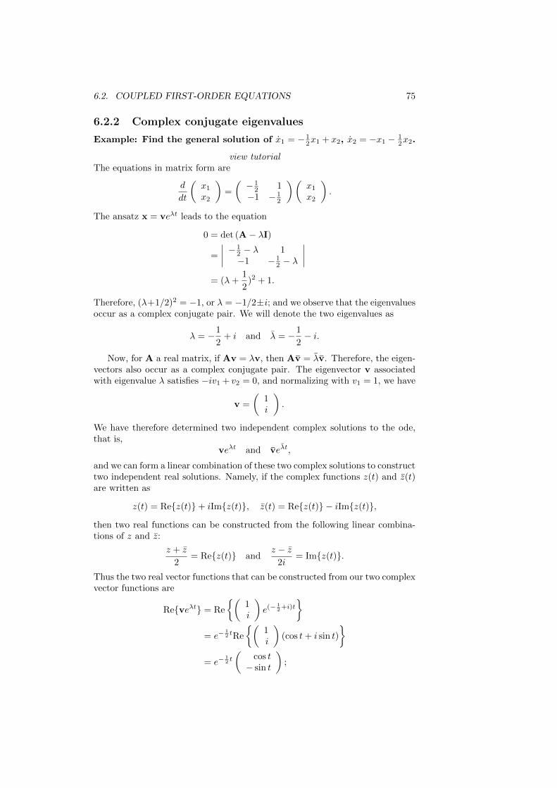
6.2. COUPLED FIRST-ORDER EQUATIONS 75
6.2.2 Complex conjugate eigenvalues
Example: Find the general solution of ��1 = − 12𝑥1 + 𝑥2, ��2 = −𝑥1 − 1
2𝑥2.
view tutorialThe equations in matrix form are
𝑑
𝑑𝑡
(𝑥1
𝑥2
)=
(− 1
2 1−1 − 1
2
)(𝑥1
𝑥2
).
The ansatz x = v𝑒𝜆𝑡 leads to the equation
0 = det (A− 𝜆I)
=
− 1
2 − 𝜆 1−1 − 1
2 − 𝜆
= (𝜆+
1
2)2 + 1.
Therefore, (𝜆+1/2)2 = −1, or 𝜆 = −1/2±𝑖; and we observe that the eigenvaluesoccur as a complex conjugate pair. We will denote the two eigenvalues as
𝜆 = −1
2+ 𝑖 and �� = −1
2− 𝑖.
Now, for A a real matrix, if Av = 𝜆v, then Av = ��v. Therefore, the eigen-vectors also occur as a complex conjugate pair. The eigenvector v associatedwith eigenvalue 𝜆 satisfies −𝑖𝑣1 + 𝑣2 = 0, and normalizing with 𝑣1 = 1, we have
v =
(1𝑖
).
We have therefore determined two independent complex solutions to the ode,that is,
v𝑒𝜆𝑡 and v𝑒��𝑡,
and we can form a linear combination of these two complex solutions to constructtwo independent real solutions. Namely, if the complex functions 𝑧(𝑡) and 𝑧(𝑡)are written as
𝑧(𝑡) = Re{𝑧(𝑡)}+ 𝑖Im{𝑧(𝑡)}, 𝑧(𝑡) = Re{𝑧(𝑡)} − 𝑖Im{𝑧(𝑡)},
then two real functions can be constructed from the following linear combina-tions of 𝑧 and 𝑧:
𝑧 + 𝑧
2= Re{𝑧(𝑡)} and
𝑧 − 𝑧
2𝑖= Im{𝑧(𝑡)}.
Thus the two real vector functions that can be constructed from our two complexvector functions are
Re{v𝑒𝜆𝑡} = Re
{(1𝑖
)𝑒(−
12+𝑖)𝑡
}= 𝑒−
12 𝑡Re
{(1𝑖
)(cos 𝑡+ 𝑖 sin 𝑡)
}= 𝑒−
12 𝑡
(cos 𝑡
− sin 𝑡
);

76 CHAPTER 6. SYSTEMS OF EQUATIONS
−2 −1.5 −1 −0.5 0 0.5 1 1.5 2−2
−1.5
−1
−0.5
0
0.5
1
1.5
2
x1
x 2
phase space diagram
Figure 6.3: Phase space diagram for example with complex conjugate eigenval-ues.
and
Im{v𝑒𝜆𝑡} = 𝑒−12 𝑡Im
{(1𝑖
)(cos 𝑡+ 𝑖 sin 𝑡)
}= 𝑒−
12 𝑡
(sin 𝑡cos 𝑡
).
Taking a linear superposition of these two real solutions yields the general so-lution to the ode, given by
x = 𝑒−12 𝑡
(𝐴
(cos 𝑡
− sin 𝑡
)+𝐵
(sin 𝑡cos 𝑡
)).
The corresponding phase space diagram is shown in Fig. 6.3. We say theorigin is a spiral point. If the real part of the complex eigenvalue is negative,as is the case here, then solutions spiral into the origin. If the real part of theeigenvalue is positive, then solutions spiral out of the origin.
The direction of the spiral—here, it is clockwise—can be determined usinga concept from physics. If a particle of unit mass moves along a phase spacetrajectory, then the angular momentum of the particle about the origin is equalto the cross product of the position and velocity vectors: L = x × x. Withboth the position and velocity vectors lying in the two-dimensional phase spaceplane, the angular momentum vector is perpendicular to this plane. With
x = (𝑥1, 𝑥2, 0), x = (��1, ��2, 0),
thenL = (0, 0, 𝐿), with 𝐿 = 𝑥1��2 − 𝑥2��1.
By the right-hand-rule, a clockwise rotation corresponds to 𝐿 < 0, and a coun-terclockwise rotation to 𝐿 > 0.

6.2. COUPLED FIRST-ORDER EQUATIONS 77
The computation of 𝐿 in our present example proceeds from the differentialequations as follows:
𝑥1��2 − 𝑥2��1 = 𝑥1(−𝑥1 −1
2𝑥2)− 𝑥2(−
1
2𝑥1 + 𝑥2)
= −(𝑥21 + 𝑥2
2)
< 0.
And since 𝐿 < 0, the spiral rotation is clockwise, as shown in Fig. 6.3.
6.2.3 Repeated eigenvalues with one eigenvector
Example: Find the general solution of ��1 = 𝑥1 − 𝑥2, ��2 = 𝑥1 + 3𝑥2.
view tutorial
The equations in matrix form are
𝑑
𝑑𝑡
(𝑥1
𝑥2
)=
(1 −11 3
)(𝑥1
𝑥2
). (6.9)
The ansatz x = v𝑒𝜆𝑡 leads to the characteristic equation
0 = det (A− 𝜆I)
= 𝜆2 − 4𝜆+ 4
= (𝜆− 2)2.
Therefore, 𝜆 = 2 is a repeated eigenvalue. The associated eigenvector is foundfrom −𝑣1 − 𝑣2 = 0, or 𝑣2 = −𝑣1; and normalizing with 𝑣1 = 1, we have
𝜆 = 2, v =
(1
−1
).
We have thus found a single solution to the ode, given by
x1(𝑡) = 𝑐1
(1
−1
)𝑒2𝑡,
and we need to find the missing second solution to be able to satisfy the initialconditions. An ansatz of 𝑡 times the first solution is tempting, but will fail. Here,we will cheat and find the missing second solution by solving the equivalentsecond-order, homogeneous, constant-coefficient differential equation.
We already know that this second-order differential equation for 𝑥1(𝑡) has acharacteristic equation with a degenerate eigenvalue given by 𝜆 = 2. Therefore,the general solution for 𝑥1 is given by
𝑥1(𝑡) = (𝑐1 + 𝑡𝑐2)𝑒2𝑡.
To determine 𝑥2, we first compute
��1 =(2𝑐1 + (1 + 2𝑡)𝑐2
)𝑒2𝑡,
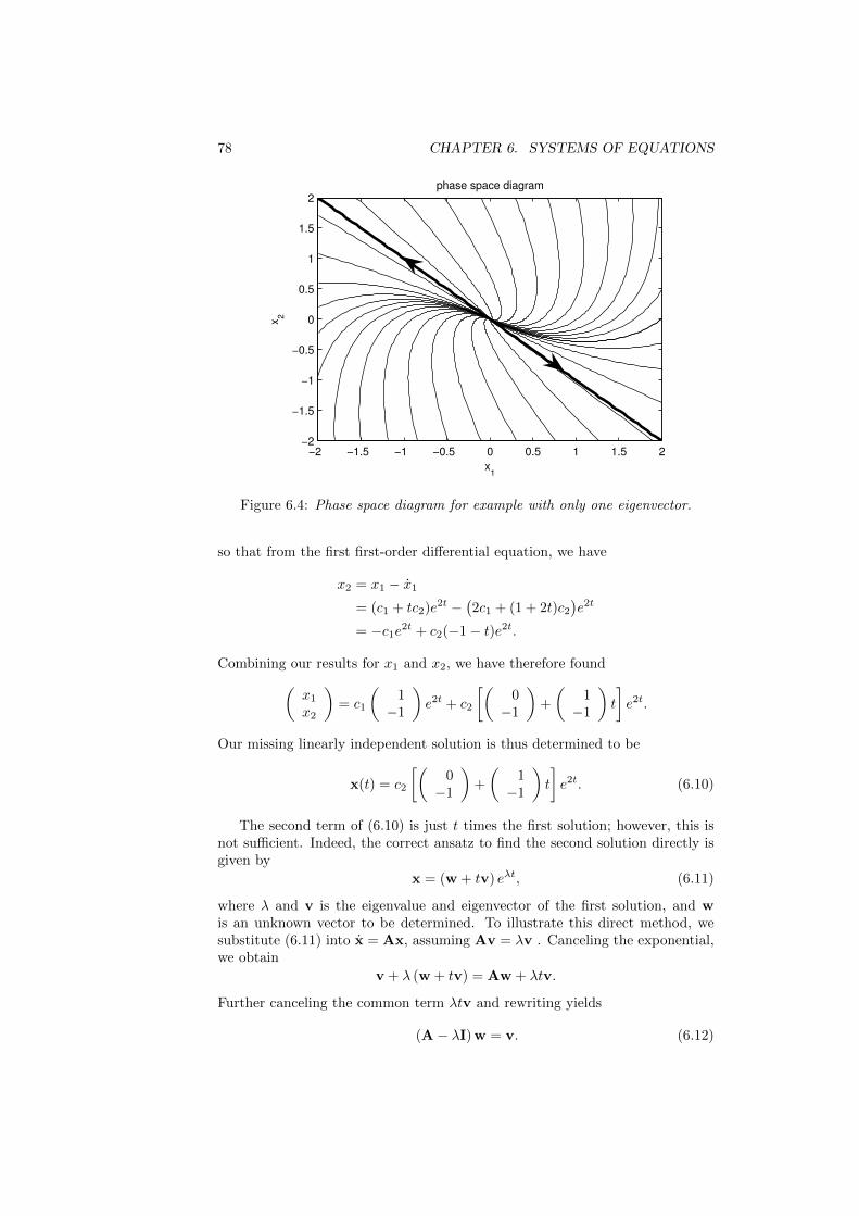
78 CHAPTER 6. SYSTEMS OF EQUATIONS
−2 −1.5 −1 −0.5 0 0.5 1 1.5 2−2
−1.5
−1
−0.5
0
0.5
1
1.5
2
x1
x 2
phase space diagram
Figure 6.4: Phase space diagram for example with only one eigenvector.
so that from the first first-order differential equation, we have
𝑥2 = 𝑥1 − ��1
= (𝑐1 + 𝑡𝑐2)𝑒2𝑡 −
(2𝑐1 + (1 + 2𝑡)𝑐2
)𝑒2𝑡
= −𝑐1𝑒2𝑡 + 𝑐2(−1− 𝑡)𝑒2𝑡.
Combining our results for 𝑥1 and 𝑥2, we have therefore found(𝑥1
𝑥2
)= 𝑐1
(1
−1
)𝑒2𝑡 + 𝑐2
[(0
−1
)+
(1
−1
)𝑡
]𝑒2𝑡.
Our missing linearly independent solution is thus determined to be
x(𝑡) = 𝑐2
[(0
−1
)+
(1
−1
)𝑡
]𝑒2𝑡. (6.10)
The second term of (6.10) is just 𝑡 times the first solution; however, this isnot sufficient. Indeed, the correct ansatz to find the second solution directly isgiven by
x = (w + 𝑡v) 𝑒𝜆𝑡, (6.11)
where 𝜆 and v is the eigenvalue and eigenvector of the first solution, and wis an unknown vector to be determined. To illustrate this direct method, wesubstitute (6.11) into x = Ax, assuming Av = 𝜆v . Canceling the exponential,we obtain
v + 𝜆 (w + 𝑡v) = Aw + 𝜆𝑡v.
Further canceling the common term 𝜆𝑡v and rewriting yields
(A− 𝜆I)w = v. (6.12)

6.3. NORMAL MODES 79
If A has only a single linearly independent eigenvector v, then (6.12) can besolved for w (otherwise, it can not). Using A, 𝜆 and v of our present example,(6.12) is the system of equations given by(
−1 −11 1
)(𝑤1
𝑤2
)=
(1
−1
).
The first and second equation are the same, so that 𝑤2 = −(𝑤1+1). Therefore,
w =
(𝑤1
−(𝑤1 + 1)
)= 𝑤1
(1
−1
)+
(0
−1
).
Notice that the first term repeats the first found solution, i.e., a constant timesthe eigenvector, and the second term is new. We therefore take 𝑤1 = 0 andobtain
w =
(0
−1
),
as before.The phase space diagram for this ode is shown in Fig. 6.4. The dark line is
the single eigenvector v of the matrixA. When there is only a single eigenvector,the origin is called an improper node.
There is a definite counterclockwise rotation to the phase space trajectories,and this can be confirmed from the calculation
𝐿 = 𝑥1��2 − 𝑥2��1
= 𝑥1(𝑥1 + 3𝑥2)− 𝑥2(𝑥1 − 𝑥2)
= 𝑥21 + 2𝑥1𝑥2 + 𝑥2
2
= (𝑥1 + 𝑥2)2
> 0.
6.3 Normal modes
view tutorial, Part 1 view tutorial, Part 2We now consider an application of the eigenvector analysis to the coupled mass-spring system shown in Fig. 6.5. The position variables 𝑥1 and 𝑥2 are measuredfrom the equilibrium positions of the masses. Hooke’s law states that the springforce is linearly proportional to the extension length of the spring, measuredfrom equilibrium. By considering the extension of the spring and the sign of theforce, we write Newton’s law 𝐹 = 𝑚𝑎 separately for each mass:
𝑚��1 = −𝑘𝑥1 − 𝑘12(𝑥1 − 𝑥2),
𝑚��2 = −𝑘𝑥2 − 𝑘12(𝑥2 − 𝑥1).
Further rewriting by collecting terms proportional to 𝑥1 and 𝑥2 yields
𝑚��1 = −(𝑘 + 𝑘12)𝑥1 + 𝑘12𝑥2,
𝑚��2 = 𝑘12𝑥1 − (𝑘 + 𝑘12)𝑥2.

80 CHAPTER 6. SYSTEMS OF EQUATIONS
Figure 6.5: Coupled harmonic oscillators (figure from Eric Weisstein’s Worldof Physics).
The equations for the coupled mass-spring system form a system of two second-order linear homogeneous odes. In matrix form, 𝑚x = Ax, or explicitly,
𝑚𝑑2
𝑑𝑡2
(𝑥1
𝑥2
)=
(−(𝑘 + 𝑘12) 𝑘12
𝑘12 −(𝑘 + 𝑘12)
)(𝑥1
𝑥2
). (6.13)
In analogy to a system of first-order equations, we try the ansatz x = v𝑒𝜆𝑡, andupon substitution into (6.13) we obtain the eigenvalue problem Av = 𝑚𝜆2v.The values of 𝑚𝜆2 are determined by solving the characteristic equation
0 = det (A−𝑚𝜆2I)
=
−(𝑘 + 𝑘12)−𝑚𝜆2 𝑘12
𝑘12 −(𝑘 + 𝑘12)−𝑚𝜆2
= (𝑚𝜆2 + 𝑘 + 𝑘12)
2 − 𝑘212.
The solution for m𝜆2 is
𝑚𝜆2 = −𝑘 − 𝑘12 ± 𝑘12,
and the two eigenvalues are
𝜆21 = −𝑘/𝑚, 𝜆2
2 = −(𝑘 + 2𝑘12)/𝑚.
Since 𝜆21, 𝜆
22 < 0, both values of 𝜆 are imaginary, and 𝑥1(𝑡) and 𝑥2(𝑡) oscillate
with angular frequencies 𝜔1 = |𝜆1| and 𝜔2 = |𝜆2|, where
𝜔1 =√𝑘/𝑚, 𝜔2 =
√(𝑘 + 2𝑘12)/𝑚.
The positions of the oscillating masses in general contain time dependencies ofthe form sin𝜔1𝑡, cos𝜔1𝑡, and sin𝜔2𝑡, cos𝜔2𝑡.
It is of further interest to determine the eigenvectors, or so-called normalmodes of oscillation, associated with the two distinct angular frequencies. Withspecific initial conditions proportional to an eigenvector, the mass will oscillatewith a single frequency. The eigenvector associated with 𝑚𝜆2
1 satisfies
−𝑘12𝑣11 + 𝑘12𝑣12 = 0,
so that 𝑣11 = 𝑣12. The normal mode associated with the frequency 𝜔1 =√𝑘/𝑚 thus follows a motion where 𝑥1 = 𝑥2. Referring to Fig. 6.5, during this

6.3. NORMAL MODES 81
motion the center spring length does not change, and the two masses oscillateas if the center spring was absent (which is why the frequency of oscillation isindependent of 𝑘12).
Next, we determine the eigenvector associated with 𝑚𝜆22:
𝑘12𝑣21 + 𝑘12𝑣22 = 0,
so that 𝑣21 = −𝑣22. The normal mode associated with the frequency 𝜔2 =√(𝑘 + 2𝑘12)/𝑚 thus follows a motion where 𝑥1 = −𝑥2. Again referring to
Fig. 6.5, during this motion the two equal masses symmetrically push or pullagainst each side of the middle spring.
A general solution for x(𝑡) can be constructed from the eigenvalues andeigenvectors. Our ansatz was x = v𝑒𝜆𝑡, and we can linearly superimpose oursolutions with the additional requirement that x is real. The final result, with𝜔1 =
√𝑘/𝑚 and 𝜔2 =
√(𝑘 + 2𝑘12)/𝑚, is(
𝑥1
𝑥2
)=
(11
)(𝐴 cos𝜔1𝑡+𝐵 sin𝜔1𝑡) +
(1
−1
)(𝐶 cos𝜔2𝑡+𝐷 sin𝜔2𝑡) ,
where the now real constants 𝐴, 𝐵, 𝐶, and 𝐷 can be determined from the fourindependent initial conditions, 𝑥1(0), 𝑥2(0), ��1(0), and ��2(0).

82 CHAPTER 6. SYSTEMS OF EQUATIONS
Chapter 7
Nonlinear differentialequations and bifurcationtheory
Reference: Strogatz, Sections 2.2, 2.4, 3.1, 3.2, 3.4, 6.3, 6.4, 8.2
view lectureWe now turn our attention to nonlinear differential equations. In particular, westudy how small changes in the parameters of a system can result in qualita-tive changes in the dynamics. These qualitative changes in the dynamics arecalled bifurcations. To understand bifurcations, we first need to understand theconcepts of fixed points and stability.
7.1 Fixed points and stability
Consider the one-dimensional differential equation for 𝑥 = 𝑥(𝑡) given by
�� = 𝑓(𝑥). (7.1)
We say that 𝑥* is a fixed point, or equilibrium point, of (7.1) if 𝑓(𝑥*) = 0. Atthe fixed point, �� = 0. The terminology fixed point is used since the solution to(7.1) with initial condition 𝑥(0) = 𝑥* is 𝑥(𝑡) = 𝑥* for all time 𝑡.
A fixed point, however, can be stable or unstable. A fixed point is said to bestable if a small perturbation of the solution from the fixed point decays in time;it is said to be unstable if a small perturbation grows in time. We can determinestability by a linear analysis. Let 𝑥 = 𝑥* + 𝜖(𝑡), where 𝜖 represents a smallperturbation of the solution from the fixed point 𝑥*. Because 𝑥* is a constant,�� = ��; and because 𝑥* is a fixed point, 𝑓(𝑥*) = 0. Taylor series expanding about𝜖 = 0, we have
�� = 𝑓(𝑥* + 𝜖)
= 𝑓(𝑥*) + 𝜖𝑓 ′(𝑥*) + . . .
= 𝜖𝑓 ′(𝑥*) + . . . .
The omitted terms in the Taylor series expansion are proportional to 𝜖2, andcan be made negligible over a short time interval with respect to the kept term,
83

84 CHAPTER 7. BIFURCATION THEORY
proportional to 𝜖, by taking 𝜖(0) sufficiently small. Therefore, at least over shorttimes, the differential equation to be considered, �� = 𝑓 ′(𝑥*)𝜖, is linear and hasby now the familiar solution
𝜖(𝑡) = 𝜖(0)𝑒𝑓′(𝑥*)𝑡.
The perturbation of the fixed point solution 𝑥(𝑡) = 𝑥* thus decays exponentiallyif 𝑓 ′(𝑥*) < 0, and we say the fixed point is stable. If 𝑓 ′(𝑥*) > 0, the perturbationgrows exponentially and we say the fixed point is unstable. If 𝑓 ′(𝑥*) = 0, wesay the fixed point is marginally stable, and the next higher-order term in theTaylor series expansion must be considered.
Example: Find all the fixed points of the logistic equation �� = 𝑥(1−𝑥)and determine their stability.
There are two fixed points at which �� = 0, given by 𝑥* = 0 and 𝑥* = 1. Stabilityof these equilibrium points may be determined by considering the derivative of𝑓(𝑥) = 𝑥(1 − 𝑥). We have 𝑓 ′(𝑥) = 1 − 2𝑥. Therefore, 𝑓 ′(0) = 1 > 0 so that𝑥* = 0 is an unstable fixed point, and 𝑓 ′(1) = −1 < 0 so that 𝑥* = 1 is a stablefixed point. Indeed, we have previously found that all solutions approach thestable fixed point asymptotically.
The idea of fixed points and stability can be extended to higher-order systemsof odes. Here, we consider a two-dimensional system and will need to make useof the two-dimensional Taylor series expansion of a function 𝐹 (𝑥, 𝑦) about theorigin. In general, the Taylor series of 𝐹 (𝑥, 𝑦) is given by
𝐹 (𝑥, 𝑦) = 𝐹 + 𝑥𝜕𝐹
𝜕𝑥+ 𝑦
𝜕𝐹
𝜕𝑦+
1
2
(𝑥2 𝜕
2𝐹
𝜕𝑥2+ 2𝑥𝑦
𝜕2𝐹
𝜕𝑥𝜕𝑦+ 𝑦2
𝜕2𝐹
𝜕𝑦2
)+ . . . ,
where the function 𝐹 and all of its partial derivatives on the right-hand-side areevaluated at the origin. Note that the Taylor series is constructed so that allpartial derivatives of the left-hand-side match those of the right-hand-side atthe origin.
We now consider the two-dimensional system given by
�� = 𝑓(𝑥, 𝑦), �� = 𝑔(𝑥, 𝑦). (7.2)
The point (𝑥*, 𝑦*) is said to be a fixed point of (7.2) if 𝑓(𝑥*, 𝑦*) = 0 and𝑔(𝑥*, 𝑦*) = 0. Again, the local stability of a fixed point can be determined bya linear analysis. We let 𝑥(𝑡) = 𝑥* + 𝜖(𝑡) and 𝑦(𝑡) = 𝑦* + 𝛿(𝑡), where 𝜖 and 𝛿are small independent perturbations from the fixed point. Making use of thetwo dimensional Taylor series of 𝑓(𝑥, 𝑦) and 𝑔(𝑥, 𝑦) about the fixed point, or

7.1. FIXED POINTS AND STABILITY 85
equivalently about (𝜖, 𝛿) = (0, 0), we have
�� = 𝑓(𝑥* + 𝜖, 𝑦* + 𝛿)
= 𝑓 + 𝜖𝜕𝑓
𝜕𝑥+ 𝛿
𝜕𝑓
𝜕𝑦+ . . .
= 𝜖𝜕𝑓
𝜕𝑥+ 𝛿
𝜕𝑓
𝜕𝑦+ . . . .
�� = 𝑔(𝑥* + 𝜖, 𝑦* + 𝛿)
= 𝑔 + 𝜖𝜕𝑔
𝜕𝑥+ 𝛿
𝜕𝑔
𝜕𝑦+ . . .
= 𝜖𝜕𝑔
𝜕𝑥+ 𝛿
𝜕𝑔
𝜕𝑦+ . . . ,
where in the Taylor series 𝑓 , 𝑔 and all their partial derivatives are evaluated atthe fixed point (𝑥*, 𝑦*). Neglecting higher-order terms in the Taylor series, wethus have a system of odes for the perturbation, given in matrix form as
𝑑
𝑑𝑡
(𝜖𝛿
)=
(𝜕𝑓𝜕𝑥
𝜕𝑓𝜕𝑦
𝜕𝑔𝜕𝑥
𝜕𝑔𝜕𝑦
)(𝜖𝛿
). (7.3)
The two-by-two matrix in (7.3) is called the Jacobian matrix at the fixed point.An eigenvalue analysis of the Jacobian matrix will typically yield two eigenvalues𝜆1 and 𝜆2. These eigenvalues may be real and distinct, complex conjugate pairs,or repeated. The fixed point is stable (all perturbations decay exponentially)if both eigenvalues have negative real parts. The fixed point is unstable (someperturbations grow exponentially) if at least one of the eigenvalues has a positivereal part. Fixed points can be further classified as stable or unstable nodes,unstable saddle points, stable or unstable spiral points, or stable or unstableimproper nodes.
Example: Find all the fixed points of the nonlinear system �� = 𝑥(3−𝑥− 2𝑦), �� = 𝑦(2− 𝑥− 𝑦), and determine their stability.
view lectureThe fixed points are determined by solving
𝑓(𝑥, 𝑦) = 𝑥(3− 𝑥− 2𝑦) = 0, 𝑔(𝑥, 𝑦) = 𝑦(2− 𝑥− 𝑦) = 0.
There are four fixed points (𝑥*, 𝑦*): (0, 0), (0, 2), (3, 0) and (1, 1). The Jacobianmatrix is given by(
𝜕𝑓𝜕𝑥
𝜕𝑓𝜕𝑦
𝜕𝑔𝜕𝑥
𝜕𝑔𝜕𝑦
)=
(3− 2𝑥− 2𝑦 −2𝑥
−𝑦 2− 𝑥− 2𝑦
).
Stability of the fixed points may be considered in turn. With J* the Jacobianmatrix evaluated at the fixed point, we have
(𝑥*, 𝑦*) = (0, 0) : J* =
(3 00 2
).

86 CHAPTER 7. BIFURCATION THEORY
0 0.5 1 1.5 2 2.5 3 3.50
0.5
1
1.5
2
2.5
x
y
phase space diagram
Figure 7.1: Phase space plot for two-dimensional nonlinear system.
The eigenvalues of J* are 𝜆 = 3, 2 so that the fixed point (0, 0) is an unstablenode. Next,
(𝑥*, 𝑦*) = (0, 2) : J* =
(−1 0−2 −2
).
The eigenvalues of J* are 𝜆 = −1,−2 so that the fixed point (0, 2) is a stablenode. Next,
(𝑥*, 𝑦*) = (3, 0) : J* =
(−3 −60 −1
).
The eigenvalues of J* are 𝜆 = −3,−1 so that the fixed point (3, 0) is also astable node. Finally,
(𝑥*, 𝑦*) = (1, 1) : J* =
(−1 −2−1 −1
).
The characteristic equation of J* is given by (−1 − 𝜆)2 − 2 = 0, so that 𝜆 =−1±
√2. Since one eigenvalue is negative and the other positive the fixed point
(1, 1) is an unstable saddle point. From our analysis of the fixed points, one canexpect that all solutions will asymptote to one of the stable fixed points (0, 2)or (3, 0), depending on the initial conditions.
It is of interest to sketch the phase space diagram for this nonlinear system.The eigenvectors associated with the unstable saddle point (1, 1) determine thedirections of the flow into and away from this fixed point. The eigenvectorassociated with the positive eigenvalue 𝜆1 = −1 +
√2 can determined from the
first equation of (J* − 𝜆1I)v1 = 0, or
−√2𝑣11 − 2𝑣12 = 0,
so that 𝑣12 = −(√2/2)𝑣11. The eigenvector associated with the negative eigen-
value 𝜆1 = −1−√2 satisfies 𝑣22 = (
√2/2)𝑣21. The eigenvectors give the slope

7.2. ONE-DIMENSIONAL BIFURCATIONS 87
of the lines with origin at the fixed point for incoming (negative eigenvalue) andoutgoing (positive eigenvalue) trajectories. The outgoing trajectories have neg-ative slope −
√2/2 and the incoming trajectories have positive slope
√2/2. A
rough sketch of the phase space diagram can be made by hand (as demonstratedin class). Here, a computer generated plot obtained from numerical solution ofthe nonlinear coupled odes is presented in Fig. 7.1. The curve starting fromthe origin and at infinity, and terminating at the unstable saddle point is calledthe separatrix. This curve separates the phase space into two regions: initialconditions for which the solution asymptotes to the fixed point (0, 2), and initialconditions for which the solution asymptotes to the fixed point (3, 0).
7.2 One-dimensional bifurcations
We now consider four classic bifurcations of one-dimensional nonlinear differ-ential equations: saddle-node bifurcation, transcritical bifurcation, supercriticalpitchfork bifurcation, and subcritical pitchfork bifurcation. The correspondingdifferential equation will be written as
�� = 𝑓𝑟(𝑥),
where the subscript 𝑟 represents a parameter that results in a bifurcation whenvaried across zero. The simplest differential equations that exhibit these bifur-cations are called the normal forms, and correspond to a local analysis (i.e.,Taylor series expansion) of more general differential equations around the fixedpoint, together with a possible rescaling of 𝑥.
7.2.1 Saddle-node bifurcation
view lectureThe saddle-node bifurcation results in fixed points being created or destroyed.The normal form for a saddle-node bifurcation is given by
�� = 𝑟 + 𝑥2.
The fixed points are 𝑥* = ±√−𝑟. Clearly, two real fixed points exist when
𝑟 < 0 and no real fixed points exist when 𝑟 > 0. The stability of the fixedpoints when 𝑟 < 0 are determined by the derivative of 𝑓(𝑥) = 𝑟 + 𝑥2, given by𝑓 ′(𝑥) = 2𝑥. Therefore, the negative fixed point is stable and the positive fixedpoint is unstable.
Graphically, we can illustrate this bifurcation in two ways. First, in Fig. 7.2(a),we plot �� versus 𝑥 for the three parameter values corresponding to 𝑟 < 0, 𝑟 = 0and 𝑟 > 0. The values at which �� = 0 correspond to the fixed points, andarrows are drawn indicating how the solution 𝑥(𝑡) evolves (to the right if �� > 0and to the left if �� < 0). The stable fixed point is indicated by a filled circleand the unstable fixed point by an open circle. Note that when 𝑟 = 0, solutionsconverge to the origin from the left, but diverge from the origin on the right.Second, in Fig. 7.2(b), we plot a bifurcation diagram illustrating the fixed point𝑥* versus the bifurcation parameter 𝑟. The stable fixed point is denoted by asolid line and the unstable fixed point by a dashed line. Note that the two fixedpoints collide and annihilate at 𝑟 = 0, and there are no fixed points for 𝑟 > 0.

88 CHAPTER 7. BIFURCATION THEORY
→ ← →
r<0
→ →
r=0 r>0
dx/dt
x
(a)
(b) x*
r
Figure 7.2: Saddlenode bifurcation. (a) �� versus 𝑥; (b) bifurcation diagram.
7.2.2 Transcritical bifurcation
view lecture
A transcritical bifurcation occurs when there is an exchange of stabilities be-tween two fixed points. The normal form for a transcritical bifurcation is givenby
�� = 𝑟𝑥− 𝑥2.
The fixed points are 𝑥* = 0 and 𝑥* = 𝑟. The derivative of the right-hand-side is𝑓 ′(𝑥) = 𝑟 − 2𝑥, so that 𝑓 ′(0) = 𝑟 and 𝑓 ′(𝑟) = −𝑟. Therefore, for 𝑟 < 0, 𝑥* = 0is stable and 𝑥* = 𝑟 is unstable, while for 𝑟 > 0, 𝑥* = 𝑟 is stable and 𝑥* = 0is unstable. The two fixed points thus exchange stability as 𝑟 passes throughzero. The transcritical bifurcation is illustrated in Fig. 7.3.
7.2.3 Supercritical pitchfork bifurcation
The pitchfork bifurcations occur in physical models where fixed points appearand disappear in pairs due to some intrinsic symmetry of the problem. Pitchforkbifurcations can come in one of two types. In the supercritical bifurcation, apair of stable fixed points are created at the bifurcation (or critical) point andexist after (super) the bifurcation. In the subcritical bifurcation, a pair ofunstable fixed points are created at the bifurcation point and exist before (sub)the bifurcation.
The normal form for the supercritical pitchfork bifurcation is given by
�� = 𝑟𝑥− 𝑥3.

7.2. ONE-DIMENSIONAL BIFURCATIONS 89
← → ←
r<0
dx/dt
x
(a)
← ←
r=0
←← →
r>0
x*
r
(b)
Figure 7.3: Transcritical bifurcation. (a) �� versus 𝑥; (b) bifurcation diagram.
Note that the linear term results in exponential growth when 𝑟 > 0 and thenonlinear term stabilizes this growth. The fixed points are 𝑥* = 0 and 𝑥* =±√𝑟, the latter fixed points existing only when 𝑟 > 0. The derivative of 𝑓 is
𝑓 ′(𝑥) = 𝑟 − 3𝑥2 so that 𝑓 ′(0) = 𝑟 and 𝑓 ′(±√𝑟) = −2𝑟. Therefore, the fixed
point 𝑥* = 0 is stable for 𝑟 < 0 and unstable for 𝑟 > 0 while the fixed points𝑥 = ±
√𝑟 exist and are stable for 𝑟 > 0. Notice that the fixed point 𝑥* = 0
becomes unstable as 𝑟 crosses zero and two new stable fixed points 𝑥* = ±√𝑟
are born. The supercritical pitchfork bifurcation is illustrated in Fig. 7.4.
7.2.4 Subcritical pitchfork bifurcation
view lecture
In the subcritical case, the cubic term is destabilizing. The normal form (toorder 𝑥3) is
�� = 𝑟𝑥+ 𝑥3.
The fixed points are 𝑥* = 0 and 𝑥* = ±√−𝑟, the latter fixed points existing
only when 𝑟 ≤ 0. The derivative of the right-hand-side is 𝑓 ′(𝑥) = 𝑟 + 3𝑥2 sothat 𝑓 ′(0) = 𝑟 and 𝑓 ′(±
√−𝑟) = −2𝑟. Therefore, the fixed point 𝑥* = 0 is stable
for 𝑟 < 0 and unstable for 𝑟 > 0 while the fixed points 𝑥 = ±√−𝑟 exist and are
unstable for 𝑟 < 0. There are no stable fixed points when 𝑟 > 0.
The absence of stable fixed points for 𝑟 > 0 indicates that the neglect ofterms of higher-order in 𝑥 than 𝑥3 in the normal form may be unwarranted.Keeping to the intrinsic symmetry of the equations (only odd powers of 𝑥) wecan add a stabilizing nonlinear term proportional to 𝑥5. The extended normal
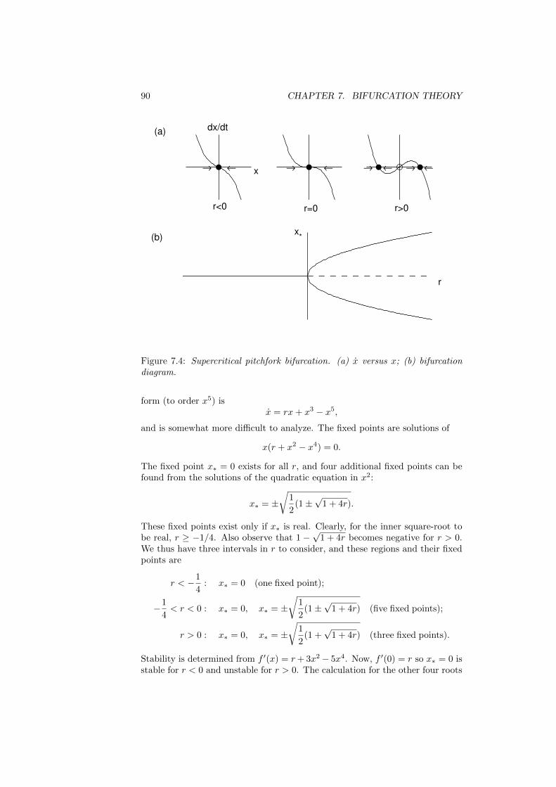
90 CHAPTER 7. BIFURCATION THEORY
→ ←
r<0
dx/dt
x
(a)
→ ←
r=0
←→ ← →
r>0
x*
r
(b)
Figure 7.4: Supercritical pitchfork bifurcation. (a) �� versus 𝑥; (b) bifurcationdiagram.
form (to order 𝑥5) is�� = 𝑟𝑥+ 𝑥3 − 𝑥5,
and is somewhat more difficult to analyze. The fixed points are solutions of
𝑥(𝑟 + 𝑥2 − 𝑥4) = 0.
The fixed point 𝑥* = 0 exists for all 𝑟, and four additional fixed points can befound from the solutions of the quadratic equation in 𝑥2:
𝑥* = ±√
1
2(1±
√1 + 4𝑟).
These fixed points exist only if 𝑥* is real. Clearly, for the inner square-root tobe real, 𝑟 ≥ −1/4. Also observe that 1 −
√1 + 4𝑟 becomes negative for 𝑟 > 0.
We thus have three intervals in 𝑟 to consider, and these regions and their fixedpoints are
𝑟 < −1
4: 𝑥* = 0 (one fixed point);
−1
4< 𝑟 < 0 : 𝑥* = 0, 𝑥* = ±
√1
2(1±
√1 + 4𝑟) (five fixed points);
𝑟 > 0 : 𝑥* = 0, 𝑥* = ±√
1
2(1 +
√1 + 4𝑟) (three fixed points).
Stability is determined from 𝑓 ′(𝑥) = 𝑟+3𝑥2 − 5𝑥4. Now, 𝑓 ′(0) = 𝑟 so 𝑥* = 0 isstable for 𝑟 < 0 and unstable for 𝑟 > 0. The calculation for the other four roots

7.2. ONE-DIMENSIONAL BIFURCATIONS 91
x*
r
Figure 7.5: Subcritical pitchfork bifurcation diagram.
can be simplified by noting that 𝑥* satisfies 𝑟 + 𝑥2* − 𝑥4
* = 0, or 𝑥4* = 𝑟 + 𝑥2
*.Therefore,
𝑓 ′(𝑥*) = 𝑟 + 3𝑥2* − 5𝑥4
*
= 𝑟 + 3𝑥2* − 5(𝑟 + 𝑥2
*)
= −4𝑟 − 2𝑥2*
= −2(2𝑟 + 𝑥2*).
With 𝑥2* = 1
2 (1±√1 + 4𝑟), we have
𝑓 ′(𝑥*) = −2
(2𝑟 +
1
2(1±
√1 + 4𝑟)
)= −
((1 + 4𝑟)±
√1 + 4𝑟
)= −
√1 + 4𝑟
(√1 + 4𝑟 ± 1
).
Clearly, the plus root is always stable since 𝑓 ′(𝑥*) < 0. The minus root existsonly for − 1
4 < 𝑟 < 0 and is unstable since 𝑓 ′(𝑥*) > 0. We summarize thestability of the various fixed points:
𝑟 < −1
4: 𝑥* = 0 (stable);
−1
4< 𝑟 < 0 : 𝑥* = 0, (stable)
𝑥* = ±√
1
2(1 +
√1 + 4𝑟) (stable);
𝑥* = ±√
1
2(1−
√1 + 4𝑟) (unstable);
𝑟 > 0 : 𝑥* = 0 (unstable)
𝑥* = ±√
1
2(1 +
√1 + 4𝑟) (stable).
The bifurcation diagram is shown in Fig. 7.5. We can imagine what happensto the solution to the ode as 𝑟 increases from negative values, supposing thereis some noise in the system so that 𝑥(𝑡) fluctuates around a stable fixed point.For 𝑟 < −1/4, the solution 𝑥(𝑡) fluctuates around the stable fixed point 𝑥* = 0.

92 CHAPTER 7. BIFURCATION THEORY
As 𝑟 increases into the range −1/4 < 𝑟 < 0, the solution will remain close tothe stable fixed point 𝑥* = 0. However, a catastrophe occurs as soon as 𝑟 > 0.The 𝑥* = 0 fixed point is lost and the solution will jump up (or down) to theonly remaining fixed point. A similar catastrophe can happen as 𝑟 decreasesfrom positive values. In this case, the jump occurs as soon as 𝑟 < −1/4. Sincethe behavior of 𝑥(𝑡) is different depending on whether we increase or decrease𝑟, we say that the system exhibits hysteresis. The existence of a subcriticalpitchfork bifurcation can be very dangerous in engineering applications sincea small change in a problem’s parameters can result in a large change in theequilibrium state. Physically, this can result in the collapse of a structure.
7.2.5 Application: a mathematical model of a fishery
view lectureWe illustrate the utility of bifurcation theory by analyzing a simple model of afishery. We utilize the logistic equation (see S2.4.5) to model a fish populationin the absence of fishing. To model fishing, we assume that the government hasestablished fishing quotas so that at most a total of 𝐶 fish per year may becaught. We assume that when the fish population is at the carrying capacityof the environment, fisherman can catch nearly their full quota. When the fishpopulation drops to lower values, fish may be harder to find and the catch ratemay fall below 𝐶, eventually going to zero as the fish population diminishes.Combining the logistic equation together with a simple model of fishing, wepropose the mathematical model
𝑑𝑁
𝑑𝑡= 𝑟𝑁
(1− 𝑁
𝐾
)− 𝐶𝑁
𝐴+𝑁, (7.4)
where 𝑁 is the fish population size, 𝑡 is time, 𝑟 is the maximum potential growthrate of the fish population, 𝐾 is the carrying capacity of the environment, 𝐶 isthe maximum rate at which fish can be caught, and 𝐴 is a constant satisfying𝐴 < 𝐾 that is used to model the idea that fish become harder to catch whenscarce.
We nondimensionalize (7.4) using 𝑥 = 𝑁/𝐾, 𝜏 = 𝑟𝑡, 𝑐 = 𝐶/𝑟𝐾, 𝛼 = 𝐴/𝐾:
𝑑𝑥
𝑑𝜏= 𝑥(1− 𝑥)− 𝑐𝑥
𝛼+ 𝑥. (7.5)
Note that 0 ≤ 𝑥 ≤ 1, 𝑐 > 0 and 0 < 𝛼 < 1. We wish to qualitatively describethe equilibrium solutions of (7.5) and the bifurcations that may occur as thenondimensional catch rate 𝑐 increases from zero. Practically, a governmentwould like to issue each year as large a catch quota as possible without adverselyaffecting the number of fish that may be caught in subsequent years.
The fixed points of (7.5) are 𝑥* = 0, valid for all 𝑐, and the solutions to𝑥2 − (1− 𝛼)𝑥+ (𝑐− 𝛼) = 0, or
𝑥* =1
2
[(1− 𝛼)±
√(1 + 𝛼)2 − 4𝑐
]. (7.6)
The fixed points given by (7.6) are real only if 𝑐 < 14 (1 +𝛼)2. Furthermore, the
minus root is greater than zero only if (1− 𝛼) >√(1 + 𝛼)2 − 4𝑐, or after some

7.2. ONE-DIMENSIONAL BIFURCATIONS 93
x*
c
1
0α (1+α)2/4
Figure 7.6: Fishery bifurcation diagram.
algebra, 𝑐 > 𝛼. We therefore need to consider three intervals over which thefollowing fixed points exist:
0 ≤ 𝑐 ≤ 𝛼 : 𝑥* = 0, 𝑥* =1
2
[(1− 𝛼) +
√(1 + 𝛼)2 − 4𝑐
];
𝛼 < 𝑐 <1
4(1 + 𝛼)2 : 𝑥* = 0, 𝑥* =
1
2
[(1− 𝛼)±
√(1 + 𝛼)2 − 4𝑐
];
𝑐 >1
4(1 + 𝛼)2 : 𝑥* = 0.
The stability of the fixed points can be determined with rigor analytically orgraphically. Here, we simply apply biological intuition together with knowledgeof the types of one dimensional bifurcations. An intuitive argument is madesimpler if we consider 𝑐 decreasing from large values. When 𝑐 is large, thatis 𝑐 > 1
4 (1 + 𝛼)2, too many fish are being caught and our intuition suggeststhat the fish population goes extinct. Therefore, in this interval, the singlefixed point 𝑥* = 0 must be stable. As 𝑐 decreases, a bifurcation occurs at𝑐 = 1
4 (1 + 𝛼)2 introducing two additional fixed points at 𝑥* = (1 − 𝛼)/2. Thetype of one dimensional bifurcation in which two fixed points are created as asquare root becomes real is a saddlenode bifurcation, and one of the fixed pointswill be stable and the other unstable. Following these fixed points as 𝑐 → 0,we observe that the plus root goes to one, which is the appropriate stable fixedpoint when there is no fishing. We therefore conclude that the plus root is stableand the minus root is unstable. As 𝑐 decreases further from this bifurcation,the minus root collides with the fixed point 𝑥* = 0 at 𝑐 = 𝛼. This appears tobe a transcritical bifurcation and assuming an exchange of stability occurs, wemust have the fixed point 𝑥* = 0 becoming unstable for 𝑐 < 𝛼. The resultingbifurcation diagram is shown in Fig. 7.6.
The purpose of simple mathematical models applied to complex ecological

94 CHAPTER 7. BIFURCATION THEORY
problems is to offer some insight. Here, we have learned that overfishing (inthe model 𝑐 > 1
4 (1 + 𝛼)2) during one year can potentially result in a suddencollapse of the fish catch in subsequent years, so that governments need to beparticularly cautious when contemplating increases in fishing quotas.
7.3 Two-dimensional bifurcations
view lecture
All the one-dimensional bifurcations can also occur in two-dimensions alongone of the directions. In addition, a new type of bifurcation can also occurin two-dimensions. Suppose there is some control parameter 𝜇. Furthermore,suppose that for 𝜇 < 0, a two-dimensional system approaches a fixed point byexponentially-damped oscillations. We know that the Jacobian matrix at thefixed point with 𝜇 < 0 will have complex conjugate eigenvalues with negative realparts. Now suppose that when 𝜇 > 0 the real parts of the eigenvalues becomepositive so that the fixed point becomes unstable. This change in stabilityof the fixed point is called a Hopf bifurcation. The Hopf bifurcation comesin two types: supercritical Hopf bifurcation and subcritical Hopf bifurcation.For the supercritical Hopf bifurcation, as 𝜇 increases slightly above zero, theresulting oscillation around the now unstable fixed point is quickly stabilized atsmall amplitude. This stable orbit is called a limit cycle. For the subcriticalHopf bifurcation, as 𝜇 increases slightly above zero, the limit cycle immediatelyjumps to large amplitude.
7.3.1 Supercritical Hopf bifurcation
A simple example of a supercritical Hopf bifurcation can be given in polarcoordinates:
�� = 𝜇𝑟 − 𝑟3,
𝜃 = 𝜔 + 𝑏𝑟2,
where 𝑥 = 𝑟 cos 𝜃 and 𝑦 = 𝑟 sin 𝜃. The parameter 𝜇 controls the stability of thefixed point at the origin, the parameter 𝜔 is the frequency of oscillation nearthe origin, and the parameter 𝑏 determines the dependence of the oscillationfrequency at larger amplitude oscillations. Although we include 𝑏 for generality,our qualitative analysis of these equations will be independent of 𝑏.
The equation for the radius is of the form of the supercritical pitchforkbifurcation. The fixed points are 𝑟* = 0 and 𝑟* =
√𝜇 (note that 𝑟 > 0), and
the former fixed point is stable for 𝜇 < 0 and the latter is stable for 𝜇 > 0. Thetransition of the eigenvalues of the Jacobian from negative real part to positivereal part can be seen if we transform these equations to cartesian coordinates.

7.3. TWO-DIMENSIONAL BIFURCATIONS 95
We have using 𝑟2 = 𝑥2 + 𝑦2,
�� = �� cos 𝜃 − 𝜃𝑟 sin 𝜃
= (𝜇𝑟 − 𝑟3) cos 𝜃 − (𝜔 + 𝑏𝑟2)𝑟 sin 𝜃
= 𝜇𝑥− (𝑥2 + 𝑦2)𝑥− 𝜔𝑦 − 𝑏(𝑥2 + 𝑦2)𝑦
= 𝜇𝑥− 𝜔𝑦 − (𝑥2 + 𝑦2)(𝑥+ 𝑏𝑦);
�� = �� sin 𝜃 + 𝜃𝑟 cos 𝜃
= (𝜇𝑟 − 𝑟3) sin 𝜃 + (𝜔 + 𝑏𝑟2)𝑟 cos 𝜃
= 𝜇𝑦 − (𝑥2 + 𝑦2)𝑦 + 𝜔𝑥+ 𝑏(𝑥2 + 𝑦2)𝑥
= 𝜔𝑥+ 𝜇𝑦 − (𝑥2 + 𝑦2)(𝑦 − 𝑏𝑥).
The stability of the origin is determined by the Jacobian matrix evaluated atthe origin. The nonlinear terms in the equation vanish and the Jacobian matrixat the origin is given by
𝐽 =
(𝜇 −𝜔𝜔 𝜇
).
The eigenvalues are the solutions of (𝜇 − 𝜆)2 + 𝜔2 = 0, or 𝜆 = 𝜇 ± 𝑖𝜔. As𝜇 increases from negative to positive values, exponentially damped oscillationschange into exponentially growing oscillations. The nonlinear terms in the equa-tions stabilize the growing oscillations into a limit cycle.
7.3.2 Subcritical Hopf bifurcation
The analogous example of a subcritical Hopf bifurcation is given by
�� = 𝜇𝑟 + 𝑟3 − 𝑟5,
𝜃 = 𝜔 + 𝑏𝑟2.
Here, the equation for the radius is of the form of the subcritical pitchforkbifurcation. As 𝜇 increases from negative to positive values, the origin becomesunstable and exponentially growing oscillations increase until the radius reachesa stable fixed point far away from the origin. In practice, it may be difficultto tell analytically if a Hopf bifurcation is supercritical or subcritical from theequations of motion. Computational solution, however, can quickly distinguishbetween the two types.

96 CHAPTER 7. BIFURCATION THEORY

Chapter 8
Partial differentialequations
Reference: Boyce and DiPrima, Chapter 10
Differential equations containing partial derivatives with two or more inde-pendent variables are called partial differential equations (pdes). These equa-tions are of fundamental scientific interest but are substantially more difficultto solve, both analytically and computationally, than odes. In this chapter, wewill derive two fundamental pdes and show how to solve them.
8.1 Derivation of the diffusion equation
view lectureTo derive the diffusion equation in one spacial dimension, we imagine a stillliquid in a long pipe of constant cross sectional area. A small quantity of dyeis placed in a cross section of the pipe and allowed to diffuse up and down thepipe. The dye diffuses from regions of higher concentration to regions of lowerconcentration. We define 𝑢(𝑥, 𝑡) to be the concentration of the dye at position𝑥 along the pipe, and we wish to find the pde satisfied by 𝑢. It is useful to keeptrack of the units of the various quantities involved in the derivation and weintroduce the bracket notation [𝑋] to mean the units of𝑋. Relevant dimensionalunits used in the derivation of the diffusion equation are mass, length, and time,denoted as 𝑚, 𝑙, and 𝑡, respectively. Assuming that the dye concentration isuniform in every cross section of the pipe, the dimensions of concentration usedhere are [𝑢] = 𝑚/𝑙. The mass of dye in the infinitesimal pipe volume locatedbetween position 𝑥1 and position 𝑥2 at time 𝑡 is given to order Δ𝑥 = 𝑥2−𝑥1 by
𝑀 = 𝑢(𝑥, 𝑡)Δ𝑥.
The mass of dye in this infinitesimal pipe volume changes by diffusion into andout of the cross sectional ends situated at position 𝑥1 and 𝑥2 (Figure 8.1).We assume the rate of diffusion is proportional to the concentration gradient,a relationship known as Fick’s law of diffusion. Fick’s law of diffusion assumesthe mass flux 𝐽 , with units [𝐽 ] = 𝑚/𝑡 across a cross section of the pipe is givenby
𝐽 = −𝐷𝑢𝑥, (8.1)
97

98 CHAPTER 8. PARTIAL DIFFERENTIAL EQUATIONS
J (x2)J (x1)
X1 X2
Figure 8.1: Derivation of the diffusion equation.
where the diffusion constant 𝐷 > 0 has units [𝐷] = 𝑙2/𝑡. The mass flux isopposite in sign to the gradient of concentration. The time rate of change in themass of dye between 𝑥1 and 𝑥2 is given by the difference between the mass fluxinto and the mass flux out of the infinitesimal cross sectional volume. When𝑢𝑥 < 0, 𝐽 > 0 and the mass flows into the volume at position 𝑥1 and out of thevolume at position 𝑥2. On the other hand, when 𝑢𝑥 > 0, 𝐽 < 0 and the massflows out of the volume at position 𝑥1 and into the volume at position 𝑥2. Inboth cases, the time rate of change of the dye mass is given by
𝑑𝑀
𝑑𝑡= 𝐽(𝑥1, 𝑡)− 𝐽(𝑥2, 𝑡),
or rewriting in terms of 𝑢(𝑥, 𝑡):
𝑢𝑡(𝑥, 𝑡)Δ𝑥 = 𝐷 (𝑢𝑥(𝑥2, 𝑡)− 𝑢𝑥(𝑥1, 𝑡)) .
Dividing by Δ𝑥 and taking the limit Δ𝑥 → 0 results in the diffusion equation:
𝑢𝑡 = 𝐷𝑢𝑥𝑥.
We note that the diffusion equation is identical to the heat conduction equation,where 𝑢 is temperature, and the constant 𝐷 (commonly written as 𝜅) is thethermal conductivity.
8.2 Derivation of the wave equation
view lectureTo derive the wave equation in one spacial dimension, we imagine an elasticstring that undergoes small amplitude transverse vibrations. We define 𝑢(𝑥, 𝑡)to be the vertical displacement of the string from the 𝑥-axis at position 𝑥 andtime 𝑡, and we wish to find the pde satisfied by 𝑢. We define 𝜌 to be theconstant mass density of the string, 𝑇 the tension of the string, and 𝜃 the anglebetween the string and the horizonal line. We consider an infinitesimal stringelement located between 𝑥1 and 𝑥2, with Δ𝑥 = 𝑥2 − 𝑥1, as shown in Fig. 8.2.The governing equations are Newton’s law of motion for the horizontal and

8.2. DERIVATION OF THE WAVE EQUATION 99
Figure 8.2: Derivation of the wave equation.
vertical acceleration of our infinitesimal string element, and we assume that thestring element only accelerates vertically. Therefore, the horizontal forces mustbalance and we have
𝑇2 cos 𝜃2 = 𝑇1 cos 𝜃1.
The vertical forces result in a vertical acceleration, and with 𝑢𝑡𝑡 the verticalacceleration of the string element and 𝜌
√Δ𝑥2 +Δ𝑢2 = 𝜌Δ𝑥
√1 + 𝑢2
𝑥 its mass,where we have used 𝑢𝑥 = Δ𝑢/Δ𝑥, exact as Δ𝑥 → 0, we have
𝜌Δ𝑥√1 + 𝑢2
𝑥𝑢𝑡𝑡 = 𝑇2 sin 𝜃2 − 𝑇1 sin 𝜃1.
We now make the assumption of small vibrations, that is Δ𝑢 ≪ Δ𝑥, or equiv-alently 𝑢𝑥 ≪ 1. Note that [𝑢] = 𝑙 so that 𝑢𝑥 is dimensionless. With thisapproximation, to leading-order in 𝑢𝑥 we have
cos 𝜃2 = cos 𝜃1 = 1,
sin 𝜃2 = 𝑢𝑥(𝑥2, 𝑡), sin 𝜃1 = 𝑢𝑥(𝑥1, 𝑡),
and √1 + 𝑢2
𝑥 = 1.
Therefore, to leading order 𝑇1 = 𝑇2 = 𝑇 , (i.e., the tension in the string isapproximately constant), and
𝜌Δ𝑥𝑢𝑡𝑡 = 𝑇 (𝑢𝑥(𝑥2, 𝑡)− 𝑢𝑥(𝑥1, 𝑡)) .
Dividing by Δ𝑥 and taking the limit Δ𝑥 → 0 results in the wave equation
𝑢𝑡𝑡 = 𝑐2𝑢𝑥𝑥,
where 𝑐2 = 𝑇/𝜌. Since [𝑇 ] = 𝑚𝑙/𝑡2 and [𝜌] = 𝑚/𝑙, we have [𝑐2] = 𝑙2/𝑡2 so that𝑐 has units of velocity.

100 CHAPTER 8. PARTIAL DIFFERENTIAL EQUATIONS
8.3 Fourier series
view tutorialOur solution of the diffusion and wave equations will require use of a Fourierseries. A periodic function 𝑓(𝑥) with period 2𝐿, can be represented as a Fourierseries in the form
𝑓(𝑥) =𝑎02
+
∞∑𝑛=1
(𝑎𝑛 cos
𝑛𝜋𝑥
𝐿+ 𝑏𝑛 sin
𝑛𝜋𝑥
𝐿
). (8.2)
Determination of the coefficients 𝑎0, 𝑎1, 𝑎2, . . . and 𝑏1, 𝑏2, 𝑏3, . . . makes use oforthogonality relations for sine and cosine. We first define the widely usedKronecker delta 𝛿𝑛𝑚 as
𝛿𝑛𝑚 =
{1 if 𝑛 = 𝑚;0 otherwise.
The orthogonality relations for 𝑛 and 𝑚 positive integers are then given withcompact notation as the integration formulas∫ 𝐿
−𝐿
cos(𝑚𝜋𝑥
𝐿
)cos(𝑛𝜋𝑥
𝐿
)𝑑𝑥 = 𝐿𝛿𝑛𝑚, (8.3)∫ 𝐿
−𝐿
sin(𝑚𝜋𝑥
𝐿
)sin(𝑛𝜋𝑥
𝐿
)𝑑𝑥 = 𝐿𝛿𝑛𝑚, (8.4)∫ 𝐿
−𝐿
cos(𝑚𝜋𝑥
𝐿
)sin(𝑛𝜋𝑥
𝐿
)𝑑𝑥 = 0. (8.5)
We illustrate the integration technique used to obtain these results. To derive(8.4), we assume that 𝑛 and 𝑚 are positive integers with 𝑛 = 𝑚, and we makeuse of the change of variables 𝜉 = 𝜋𝑥/𝐿:∫ 𝐿
−𝐿
sin(𝑚𝜋𝑥
𝐿
)sin(𝑛𝜋𝑥
𝐿
)𝑑𝑥
=𝐿
𝜋
∫ 𝜋
−𝜋
sin (𝑚𝜉) sin (𝑛𝜉)𝑑𝜉
=𝐿
2𝜋
∫ 𝜋
−𝜋
[cos((𝑚− 𝑛)𝜉
)− cos
((𝑚+ 𝑛)𝜉
)]𝑑𝜉
=𝐿
2𝜋
[1
𝑚− 𝑛sin((𝑚− 𝑛)𝜉
)− 1
𝑚+ 𝑛sin((𝑚+ 𝑛)𝜉
)]𝜋−𝜋
= 0.
For 𝑚 = 𝑛, however,∫ 𝐿
−𝐿
sin2(𝑛𝜋𝑥
𝐿
)𝑑𝑥 =
𝐿
𝜋
∫ 𝜋
−𝜋
sin2 (𝑛𝜉)𝑑𝜉
=𝐿
2𝜋
∫ 𝜋
−𝜋
(1− cos (2𝑛𝜉)
)𝑑𝜉
=𝐿
2𝜋
[𝜉 − 1
2𝑛sin 2𝑛𝜉
]𝜋−𝜋
= 𝐿.

8.3. FOURIER SERIES 101
Integration formulas given by (8.3) and (8.5) can be similarly derived.To determine the coefficient 𝑎𝑛, we multiply both sides of (8.2) by cos (𝑛𝜋𝑥/𝐿)
with 𝑛 a nonnegative integer (changing the dummy summation variable from 𝑛to 𝑚) and integrate over 𝑥 from −𝐿 to 𝐿, assuming that the integration can bedone term by term in the infinite sum:
∫ 𝐿
−𝐿
𝑓(𝑥) cos𝑛𝜋𝑥
𝐿𝑑𝑥 =
𝑎02
∫ 𝐿
−𝐿
cos𝑛𝜋𝑥
𝐿𝑑𝑥
+
∞∑𝑚=1
{𝑎𝑚
∫ 𝐿
−𝐿
cos𝑛𝜋𝑥
𝐿cos
𝑚𝜋𝑥
𝐿𝑑𝑥+ 𝑏𝑚
∫ 𝐿
−𝐿
cos𝑛𝜋𝑥
𝐿sin
𝑚𝜋𝑥
𝐿𝑑𝑥
}.
If 𝑛 = 0, then the second and third integrals on the right-hand-side are zerobecause the cosine and sine have period 2𝐿, the integrand in the first integral onthe right-hand-side is a constant, and the right-hand-side becomes 𝐿𝑎0. If 𝑛 isa positive integer, then the first integral on the right-hand-side is zero becausethe cosine has period 2𝐿 and the third integral on the right-hand-side is zerobecause of the orthogonality of cosine and sine, (8.5). The second integral onthe right-hand-side is performed using (8.3) to obtain∫ 𝐿
−𝐿
𝑓(𝑥) cos𝑛𝜋𝑥
𝐿𝑑𝑥 =
∞∑𝑚=1
𝐿𝑎𝑚𝛿𝑛𝑚
= 𝐿𝑎𝑛,
where all the terms in the summation except 𝑚 = 𝑛 are zero by virtue of theKronecker delta. We therefore obtain for 𝑛 = 0, 1, 2, . . .
𝑎𝑛 =1
𝐿
∫ 𝐿
−𝐿
𝑓(𝑥) cos𝑛𝜋𝑥
𝐿𝑑𝑥. (8.6)
To determine the coefficients 𝑏1, 𝑏2, 𝑏3, . . . , we multiply both sides of (8.2) bysin (𝑛𝜋𝑥/𝐿) with 𝑛 a positive integer (again changing the dummy summationvariable from 𝑛 to 𝑚) and integrate:
∫ 𝐿
−𝐿
𝑓(𝑥) sin𝑛𝜋𝑥
𝐿𝑑𝑥 =
𝑎02
∫ 𝐿
−𝐿
sin𝑛𝜋𝑥
𝐿𝑑𝑥
+
∞∑𝑚=1
{𝑎𝑚
∫ 𝐿
−𝐿
sin𝑛𝜋𝑥
𝐿cos
𝑚𝜋𝑥
𝐿𝑑𝑥+ 𝑏𝑚
∫ 𝐿
−𝐿
sin𝑛𝜋𝑥
𝐿sin
𝑚𝜋𝑥
𝐿𝑑𝑥
}.
The first integral on the right-hand-side is zero because of the periodicity ofsine and the second integral on the right-hand-side is zero because of the or-thogonality of cosine and sine, (8.5). The third integral on the right-hand-sideis performed using (8.4) to obtain∫ 𝐿
−𝐿
𝑓(𝑥) sin𝑛𝜋𝑥
𝐿𝑑𝑥 =
∞∑𝑚=1
𝐿𝑏𝑚𝛿𝑛𝑚
= 𝐿𝑏𝑛,
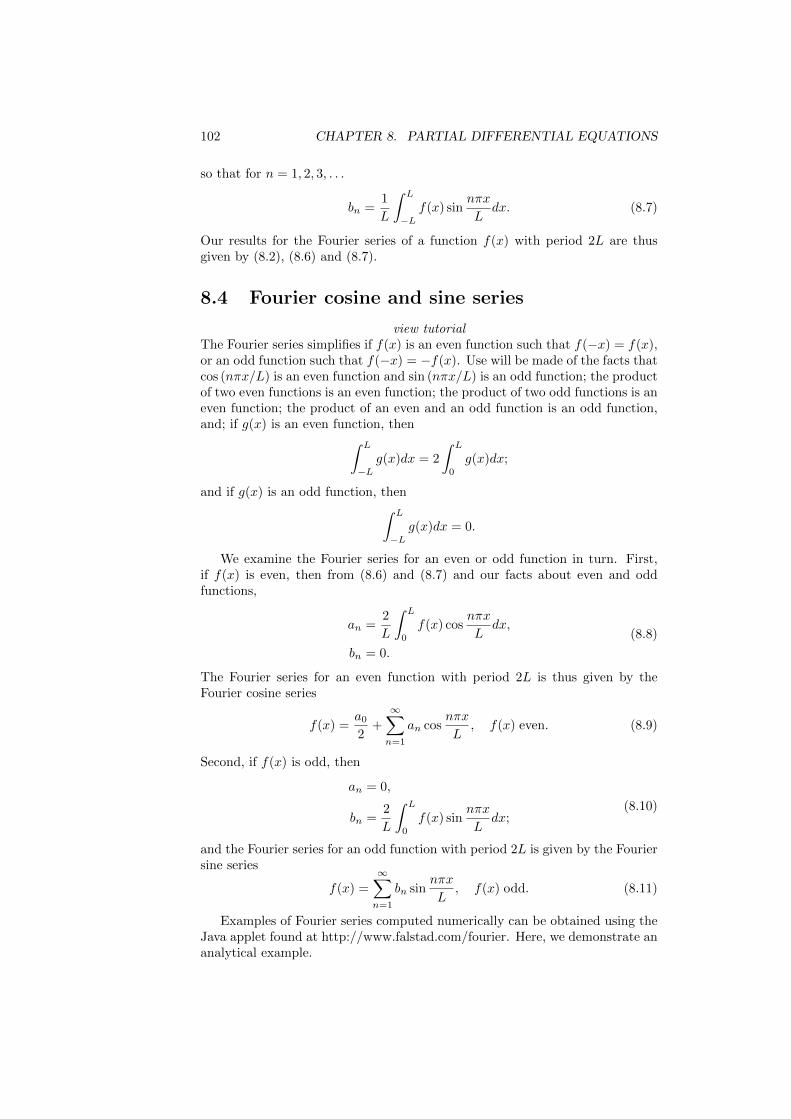
102 CHAPTER 8. PARTIAL DIFFERENTIAL EQUATIONS
so that for 𝑛 = 1, 2, 3, . . .
𝑏𝑛 =1
𝐿
∫ 𝐿
−𝐿
𝑓(𝑥) sin𝑛𝜋𝑥
𝐿𝑑𝑥. (8.7)
Our results for the Fourier series of a function 𝑓(𝑥) with period 2𝐿 are thusgiven by (8.2), (8.6) and (8.7).
8.4 Fourier cosine and sine series
view tutorialThe Fourier series simplifies if 𝑓(𝑥) is an even function such that 𝑓(−𝑥) = 𝑓(𝑥),or an odd function such that 𝑓(−𝑥) = −𝑓(𝑥). Use will be made of the facts thatcos (𝑛𝜋𝑥/𝐿) is an even function and sin (𝑛𝜋𝑥/𝐿) is an odd function; the productof two even functions is an even function; the product of two odd functions is aneven function; the product of an even and an odd function is an odd function,and; if 𝑔(𝑥) is an even function, then∫ 𝐿
−𝐿
𝑔(𝑥)𝑑𝑥 = 2
∫ 𝐿
0
𝑔(𝑥)𝑑𝑥;
and if 𝑔(𝑥) is an odd function, then∫ 𝐿
−𝐿
𝑔(𝑥)𝑑𝑥 = 0.
We examine the Fourier series for an even or odd function in turn. First,if 𝑓(𝑥) is even, then from (8.6) and (8.7) and our facts about even and oddfunctions,
𝑎𝑛 =2
𝐿
∫ 𝐿
0
𝑓(𝑥) cos𝑛𝜋𝑥
𝐿𝑑𝑥,
𝑏𝑛 = 0.
(8.8)
The Fourier series for an even function with period 2𝐿 is thus given by theFourier cosine series
𝑓(𝑥) =𝑎02
+
∞∑𝑛=1
𝑎𝑛 cos𝑛𝜋𝑥
𝐿, 𝑓(𝑥) even. (8.9)
Second, if 𝑓(𝑥) is odd, then
𝑎𝑛 = 0,
𝑏𝑛 =2
𝐿
∫ 𝐿
0
𝑓(𝑥) sin𝑛𝜋𝑥
𝐿𝑑𝑥;
(8.10)
and the Fourier series for an odd function with period 2𝐿 is given by the Fouriersine series
𝑓(𝑥) =
∞∑𝑛=1
𝑏𝑛 sin𝑛𝜋𝑥
𝐿, 𝑓(𝑥) odd. (8.11)
Examples of Fourier series computed numerically can be obtained using theJava applet found at http://www.falstad.com/fourier. Here, we demonstrate ananalytical example.

8.4. FOURIER COSINE AND SINE SERIES 103
−2*pi −pi 0 pi 2*pi−1
0
1
Figure 8.3: The even triangle function.
Example: Determine the Fourier cosine series of the even trianglefunction represented by Fig. 8.3.
view tutorial
The triangle function depicted in Fig. 8.3 is an even function of 𝑥 with period2𝜋 (i.e., 𝐿 = 𝜋). Its definition on 0 < 𝑥 < 𝜋 is given by
𝑓(𝑥) = 1− 2𝑥
𝜋.
Because 𝑓(𝑥) is even, it can be represented by the Fourier cosine series given by(8.8) and (8.9). The coefficient 𝑎0 is
𝑎0 =2
𝜋
∫ 𝜋
0
𝑓(𝑥)𝑑𝑥
=2
𝜋
∫ 𝜋
0
(1− 2𝑥
𝜋
)𝑑𝑥
=2
𝜋
[𝑥− 𝑥2
𝜋
]𝜋0
= 0.

104 CHAPTER 8. PARTIAL DIFFERENTIAL EQUATIONS
The coefficients for 𝑛 > 0 are
𝑎𝑛 =2
𝜋
∫ 𝜋
0
𝑓(𝑥) cos (𝑛𝑥)𝑑𝑥
=2
𝜋
∫ 𝜋
0
(1− 2𝑥
𝜋
)cos (𝑛𝑥)𝑑𝑥
=2
𝜋
∫ 𝜋
0
cos (𝑛𝑥)𝑑𝑥− 4
𝜋2
∫ 𝜋
0
𝑥 cos (𝑛𝑥)𝑑𝑥
=2
𝑛𝜋sin(𝑛𝑥)
]𝜋0− 4
𝜋2
{[𝑥𝑛sin (𝑛𝑥)
]𝜋0− 1
𝑛
∫ 𝜋
0
sin (𝑛𝑥)𝑑𝑥
}=
4
𝑛𝜋2
∫ 𝜋
0
sin (𝑛𝑥)𝑑𝑥
= − 4
𝑛2𝜋2cos (𝑛𝑥)
]𝜋0
=4
𝑛2𝜋2
(1− cos (𝑛𝜋)
).
Since
cos (𝑛𝜋) =
{−1, if 𝑛 odd;1, if 𝑛 even;
we have
𝑎𝑛 =
{8/(𝑛2𝜋2), if 𝑛 odd;0, if 𝑛 even.
The Fourier cosine series for the triangle function is therefore given by
𝑓(𝑥) =8
𝜋2
(cos𝑥+
cos 3𝑥
32+
cos 5𝑥
52+ . . .
).
Convergence of this series is rapid. As an interesting aside, evaluation of thisseries at 𝑥 = 0, using 𝑓(0) = 1, yields an infinite series for 𝜋2/8:
𝜋2
8= 1 +
1
32+
1
52+ . . . .
With Fourier series now included in our applied mathematics toolbox, weare ready to solve the diffusion and wave equations in bounded domains.
8.5 Solution of the diffusion equation
8.5.1 Homogeneous boundary conditions
view lectureview lecture
We consider one dimensional diffusion in a pipe of length 𝐿, and solve thediffusion equation for the concentration 𝑢(𝑥, 𝑡),
𝑢𝑡 = 𝐷𝑢𝑥𝑥, 0 ≤ 𝑥 ≤ 𝐿, 𝑡 > 0. (8.12)
Both initial and boundary conditions are required for a unique solution. Thatis, we assume the initial concentration distribution in the pipe is given by
𝑢(𝑥, 0) = 𝑓(𝑥), 0 ≤ 𝑥 ≤ 𝐿. (8.13)

8.5. SOLUTION OF THE DIFFUSION EQUATION 105
Furthermore, we assume that boundary conditions are given at the ends ofthe pipes. When the concentration value is specified at the boundaries, theboundary conditions are called Dirichlet boundary conditions. As the simplestexample, we assume here homogeneous Dirichlet boundary conditions, that iszero concentration of dye at the ends of the pipe, which could occur if the endsof the pipe open up into large reservoirs of clear solution,
𝑢(0, 𝑡) = 0, 𝑢(𝐿, 𝑡) = 0, 𝑡 > 0. (8.14)
We will later also discuss inhomogeneous Dirichlet boundary conditions andhomogeneous Neumann boundary conditions, for which the derivative of theconcentration is specified to be zero at the boundaries. Note that if 𝑓(𝑥) isidentically zero, then the trivial solution 𝑢(𝑥, 𝑡) = 0 satisfies the differentialequation and the initial and boundary conditions and is therefore the uniquesolution of the problem. In what follows, we will assume that 𝑓(𝑥) is not iden-tically zero so that we need to find a solution different than the trivial solution.
The solution method we use is called separation of variables. We assumethat 𝑢(𝑥, 𝑡) can be written as a product of two other functions, one dependentonly on position 𝑥 and the other dependent only on time 𝑡. That is, we makethe ansatz
𝑢(𝑥, 𝑡) = 𝑋(𝑥)𝑇 (𝑡). (8.15)
Whether this ansatz will succeed depends on whether the solution indeed hasthis form. Substituting (8.15) into (8.12), we obtain
𝑋𝑇 ′ = 𝐷𝑋 ′′𝑇,
which we rewrite by separating the 𝑥 and 𝑡 dependence to opposite sides of theequation:
𝑋 ′′
𝑋=
1
𝐷
𝑇 ′
𝑇.
The left hand side of this equation is independent of 𝑡 and the right hand side isindependent of 𝑥. Both sides of this equation are therefore independent of both𝑥 and 𝑡 and equal to a constant. Introducing −𝜆 as the separation constant, wehave
𝑋 ′′
𝑋=
1
𝐷
𝑇 ′
𝑇= −𝜆,
and we obtain the two ordinary differential equations
𝑋 ′′ + 𝜆𝑋 = 0, 𝑇 ′ + 𝜆𝐷𝑇 = 0. (8.16)
Because of the boundary conditions, we must first consider the equation for𝑋(𝑥). To solve, we need to determine the boundary conditions at 𝑥 = 0 and𝑥 = 𝐿. Now, from (8.14) and (8.15),
𝑢(0, 𝑡) = 𝑋(0)𝑇 (𝑡) = 0, 𝑡 > 0.
Since 𝑇 (𝑡) is not identically zero for all 𝑡 (which would result in the trivialsolution for 𝑢), we must have 𝑋(0) = 0. Similarly, the boundary condition at𝑥 = 𝐿 requires 𝑋(𝐿) = 0. We therefore consider the two-point boundary valueproblem
𝑋 ′′ + 𝜆𝑋 = 0, 𝑋(0) = 𝑋(𝐿) = 0. (8.17)
106 CHAPTER 8. PARTIAL DIFFERENTIAL EQUATIONS
The equation given by (8.17) is called an ode eigenvalue problem. The allowedvalues of 𝜆 and the corresponding functions 𝑋(𝑥) are called the eigenvalues andeigenfunctions of the differential equation. Since the form of the general solutionof the ode depends on the sign of 𝜆, we consider in turn the cases 𝜆 > 0, 𝜆 < 0and 𝜆 = 0. For 𝜆 > 0, we write 𝜆 = 𝜇2 and determine the general solution of
𝑋 ′′ + 𝜇2𝑋 = 0
to be𝑋(𝑥) = 𝐴 cos𝜇𝑥+𝐵 sin𝜇𝑥.
Applying the boundary condition at 𝑥 = 0, we find 𝐴 = 0. The boundarycondition at 𝑥 = 𝐿 then yields
𝐵 sin𝜇𝐿 = 0.
The solution 𝐵 = 0 results in the trivial solution for 𝑢 and can be ruled out.Therefore, we must have
sin𝜇𝐿 = 0,
which is an equation for the eigenvalue 𝜇. The solutions are
𝜇 = 𝑛𝜋/𝐿,
where 𝑛 is an integer. We have thus determined the eigenvalues 𝜆 = 𝜇2 > 0 tobe
𝜆𝑛 = (𝑛𝜋/𝐿)2, 𝑛 = 1, 2, 3, . . . , (8.18)
with corresponding eigenfunctions
𝑋𝑛 = sin (𝑛𝜋𝑥/𝐿). (8.19)
For 𝜆 < 0, we write 𝜆 = −𝜇2 and determine the general solution of
𝑋 ′′ − 𝜇2𝑋 = 0
to be𝑋(𝑥) = 𝐴 cosh𝜇𝑥+𝐵 sinh𝜇𝑥,
where we have previously introduced the hyperbolic sine and cosine functionsin S3.4.1. Applying the boundary condition at 𝑥 = 0, we find 𝐴 = 0. Theboundary condition at 𝑥 = 𝐿 then yields
𝐵 sinh𝜇𝐿 = 0,
which for 𝜇 = 0 has only the solution 𝐵 = 0. Therefore, there is no nontrivialsolution for 𝑢 with 𝜆 < 0. Finally, for 𝜆 = 0, we have
𝑋 ′′ = 0,
with general solution𝑋(𝑥) = 𝐴+𝐵𝑥.
The boundary condition at 𝑥 = 0 and 𝑥 = 𝐿 yields 𝐴 = 𝐵 = 0 so again there isno nontrivial solution for 𝑢 with 𝜆 = 0.

8.5. SOLUTION OF THE DIFFUSION EQUATION 107
We now turn to the equation for 𝑇 (𝑡). The equation corresponding to theeigenvalue 𝜆𝑛, using (8.18), is given by
𝑇 ′ +(𝑛2𝜋2𝐷/𝐿2
)𝑇 = 0,
which has solution proportional to
𝑇𝑛 = 𝑒−𝑛2𝜋2𝐷𝑡/𝐿2
. (8.20)
Therefore, multiplying the solutions given by (8.19) and (8.20), we concludethat the functions
𝑢𝑛(𝑥, 𝑡) = sin (𝑛𝜋𝑥/𝐿)𝑒−𝑛2𝜋2𝐷𝑡/𝐿2
(8.21)
satisfy the pde given by (8.12) and the boundary conditions given by (8.14) forevery positive integer 𝑛.
The principle of linear superposition for homogeneous linear differentialequations then states that the general solution to (8.12) and (8.14) is givenby
𝑢(𝑥, 𝑡) =
∞∑𝑛=1
𝑏𝑛𝑢𝑛(𝑥, 𝑡)
=
∞∑𝑛=1
𝑏𝑛 sin (𝑛𝜋𝑥/𝐿)𝑒−𝑛2𝜋2𝐷𝑡/𝐿2
.
(8.22)
The final solution step is to satisfy the initial conditions given by (8.13). At𝑡 = 0, we have
𝑓(𝑥) =
∞∑𝑛=1
𝑏𝑛 sin (𝑛𝜋𝑥/𝐿). (8.23)
We immediately recognize (8.23) as a Fourier sine series (8.11) for an odd func-tion 𝑓(𝑥) with period 2𝐿. Equation (8.23) is a periodic extension of our original𝑓(𝑥) defined on 0 ≤ 𝑥 ≤ 𝐿, and is an odd function because of the boundarycondition 𝑓(0) = 0. From our solution for the coefficients of a Fourier sine series(8.10), we determine
𝑏𝑛 =2
𝐿
∫ 𝐿
0
𝑓(𝑥) sin𝑛𝜋𝑥
𝐿𝑑𝑥. (8.24)
Thus the solution to the diffusion equation with homogeneous Dirichlet bound-ary conditions defined by (8.12), (8.13) and (8.14) is given by (8.22) with the𝑏𝑛 coefficients computed from (8.24).
Example: Determine the concentration of a dye in a pipe of length 𝐿,where the dye has unit mass and is initially concentrated at the centerof the pipe, and the ends of the pipe are held at zero concentration
The governing equation for concentration is the diffusion equation. We modelthe initial concentration of the dye by a delta-function centered at 𝑥 = 𝐿/2,

108 CHAPTER 8. PARTIAL DIFFERENTIAL EQUATIONS
that is, 𝑢(𝑥, 0) = 𝑓(𝑥) = 𝛿(𝑥− 𝐿/2). Therefore, from (8.24),
𝑏𝑛 =2
𝐿
∫ 𝐿
0
𝛿(𝑥− 𝐿
2) sin
𝑛𝜋𝑥
𝐿𝑑𝑥
=2
𝐿sin (𝑛𝜋/2)
=
⎧⎨⎩ 2/𝐿 if 𝑛 = 1, 5, 9, . . . ;−2/𝐿 if 𝑛 = 3, 7, 11, . . . ;0 if 𝑛 = 2, 4, 6, . . . .
With 𝑏𝑛 determined, the solution for 𝑢(𝑥, 𝑡) given by (8.22) can be written as
𝑢(𝑥, 𝑡) =2
𝐿
∞∑𝑛=0
(−1)𝑛 sin
((2𝑛+ 1)𝜋𝑥
𝐿
)𝑒−(2𝑛+1)2𝜋2𝐷𝑡/𝐿2
.
When 𝑡 ≫ 𝐿2/𝐷, the leading-order term in the series is a good approximationand is given by
𝑢(𝑥, 𝑡) ≈ 2
𝐿sin (𝜋𝑥/𝐿)𝑒−𝜋2𝐷𝑡/𝐿2
.
8.5.2 Inhomogeneous boundary conditions
view lectureConsider a diffusion problem where one end of the pipe has dye of concentrationheld constant at 𝐶1 and the other held constant at 𝐶2, which could occur if theends of the pipe had large reservoirs of fluid with different concentrations ofdye. With 𝑢(𝑥, 𝑡) the concentration of dye, the boundary conditions are givenby
𝑢(0, 𝑡) = 𝐶1, 𝑢(𝐿, 𝑡) = 𝐶2, 𝑡 > 0.
The concentration 𝑢(𝑥, 𝑡) satisfies the diffusion equation with diffusivity 𝐷:
𝑢𝑡 = 𝐷𝑢𝑥𝑥.
If we try to solve this problem directly using separation of variables, we willrun into trouble. Applying the inhomogeneous boundary condition at 𝑥 = 0directly to the ansatz 𝑢(𝑥, 𝑡) = 𝑋(𝑥)𝑇 (𝑡) results in
𝑢(0, 𝑡) = 𝑋(0)𝑇 (𝑡) = 𝐶1;
so that𝑋(0) = 𝐶1/𝑇 (𝑡).
However, our separation of variables ansatz assumes 𝑋(𝑥) to be independent of𝑡! We therefore say that inhomogeneous boundary conditions are not separable.
The proper way to solve a problem with inhomogeneous boundary conditionsis to transform it into another problem with homogeneous boundary conditions.As 𝑡 → ∞, we assume that a stationary concentration distribution 𝑣(𝑥) willattain, independent of 𝑡. Since 𝑣(𝑥) must satisfy the diffusion equation, we have
𝑣′′(𝑥) = 0, 0 ≤ 𝑥 ≤ 𝐿,
with general solution𝑣(𝑥) = 𝐴+𝐵𝑥.

8.5. SOLUTION OF THE DIFFUSION EQUATION 109
Since 𝑣(𝑥) must satisfy the same boundary conditions of 𝑢(𝑥, 𝑡), we have 𝑣(0) =𝐶1 and 𝑣(𝐿) = 𝐶2, and we determine 𝐴 = 𝐶1 and 𝐵 = (𝐶2 − 𝐶1)/𝐿.
We now express 𝑢(𝑥, 𝑡) as the sum of the known asymptotic stationary con-centration distribution 𝑣(𝑥) and an unknown transient concentration distribu-tion 𝑤(𝑥, 𝑡):
𝑢(𝑥, 𝑡) = 𝑣(𝑥) + 𝑤(𝑥, 𝑡).
Substituting into the diffusion equation, we obtain
𝜕
𝜕𝑡(𝑣(𝑥) + 𝑤(𝑥, 𝑡)) = 𝐷
𝜕2
𝜕𝑥2(𝑣(𝑥) + 𝑤(𝑥, 𝑡))
or
𝑤𝑡 = 𝐷𝑤𝑥𝑥,
since 𝑣𝑡 = 0 and 𝑣𝑥𝑥 = 0. The boundary conditions satisfied by 𝑤 are
𝑤(0, 𝑡) = 𝑢(0, 𝑡)− 𝑣(0) = 0,
𝑤(𝐿, 𝑡) = 𝑢(𝐿, 𝑡)− 𝑣(𝐿) = 0,
so that 𝑤 is observed to satisfy homogeneous boundary conditions. If the initialconditions are given by 𝑢(𝑥, 0) = 𝑓(𝑥), then the initial conditions for 𝑤 are
𝑤(𝑥, 0) = 𝑢(𝑥, 0)− 𝑣(𝑥)
= 𝑓(𝑥)− 𝑣(𝑥).
The resulting equations may then be solved for 𝑤(𝑥, 𝑡) using the technique forhomogeneous boundary conditions, and 𝑢(𝑥, 𝑡) subsequently determined.
8.5.3 Pipe with closed ends
view lectureview lecture
There is no diffusion of dye through the ends of a sealed pipe. Accordingly,the mass flux of dye through the pipe ends, given by (8.1), is zero so that theboundary conditions on the dye concentration 𝑢(𝑥, 𝑡) becomes
𝑢𝑥(0, 𝑡) = 0, 𝑢𝑥(𝐿, 𝑡) = 0, 𝑡 > 0, (8.25)
which are known as homogeneous Neumann boundary conditions. Again, weapply the method of separation of variables and as before, we obtain the twoordinary differential equations given by (8.16). Considering first the equationfor 𝑋(𝑥), the appropriate boundary conditions are now on the first derivativeof 𝑋(𝑥), and we must solve
𝑋 ′′ + 𝜆𝑋 = 0, 𝑋 ′(0) = 𝑋 ′(𝐿) = 0. (8.26)
Again, we consider in turn the cases 𝜆 > 0, 𝜆 < 0 and 𝜆 = 0. For 𝜆 > 0, wewrite 𝜆 = 𝜇2 and determine the general solution of (8.26) to be
𝑋(𝑥) = 𝐴 cos𝜇𝑥+𝐵 sin𝜇𝑥,
so that taking the derivative
𝑋 ′(𝑥) = −𝜇𝐴 sin𝜇𝑥+ 𝜇𝐵 cos𝜇𝑥.

110 CHAPTER 8. PARTIAL DIFFERENTIAL EQUATIONS
Applying the boundary condition 𝑋 ′(0) = 0, we find 𝐵 = 0. The boundarycondition at 𝑥 = 𝐿 then yields
−𝜇𝐴 sin𝜇𝐿 = 0.
The solution 𝐴 = 0 results in the trivial solution for 𝑢 and can be ruled out.Therefore, we must have
sin𝜇𝐿 = 0,
with solutions𝜇 = 𝑛𝜋/𝐿,
where 𝑛 is an integer. We have thus determined the eigenvalues 𝜆 = 𝜇2 > 0 tobe
𝜆𝑛 = (𝑛𝜋/𝐿)2, 𝑛 = 1, 2, 3, . . . , (8.27)
with corresponding eigenfunctions
𝑋𝑛 = cos (𝑛𝜋𝑥/𝐿). (8.28)
For 𝜆 < 0, we write 𝜆 = −𝜇2 and determine the general solution of (8.26) to be
𝑋(𝑥) = 𝐴 cosh𝜇𝑥+𝐵 sinh𝜇𝑥,
so that taking the derivative
𝑋 ′(𝑥) = 𝜇𝐴 sinh𝜇𝑥+ 𝜇𝐵 cosh𝜇𝑥.
Applying the boundary condition 𝑋 ′(0) = 0 yields 𝐵 = 0. The boundarycondition 𝑋 ′(𝐿) = 0 then yields
𝜇𝐴 sinh𝜇𝐿 = 0,
which for 𝜇 = 0 has only the solution 𝐴 = 0. Therefore, there is no nontrivialsolution for 𝑢 with 𝜆 < 0. Finally, for 𝜆 = 0, the general solution of (8.26) is
𝑋(𝑥) = 𝐴+𝐵𝑥,
so that taking the derivative𝑋 ′(𝑥) = 𝐵.
The boundary condition 𝑋 ′(0) = 0 yields 𝐵 = 0; 𝑋 ′(𝐿) = 0 is then triviallysatisfied. Therefore, we have an additional eigenvalue and eigenfunction givenby
𝜆0 = 0, 𝑋0(𝑥) = 1,
which can be seen as extending the formula obtained for eigenvalues and eigen-vectors for positive 𝜆 given by (8.27) and (8.28) to 𝑛 = 0.
We now turn to the equation for 𝑇 (𝑡). The equation corresponding to eigen-value 𝜆𝑛, using (8.27), is given by
𝑇 ′ +(𝑛2𝜋2𝐷/𝐿2
)𝑇 = 0,
which has solution proportional to
𝑇𝑛 = 𝑒−𝑛2𝜋2𝐷𝑡/𝐿2
, (8.29)

8.5. SOLUTION OF THE DIFFUSION EQUATION 111
valid for 𝑛 = 0, 1, 2, . . . . Therefore, multiplying the solutions given by (8.28)and (8.29), we conclude that the functions
𝑢𝑛(𝑥, 𝑡) = cos (𝑛𝜋𝑥/𝐿)𝑒−𝑛2𝜋2𝐷𝑡/𝐿2
(8.30)
satisfy the pde given by (8.12) and the boundary conditions given by (8.25) forevery nonnegative integer 𝑛.
The principle of linear superposition then yields the general solution as
𝑢(𝑥, 𝑡) =
∞∑𝑛=0
𝑐𝑛𝑢𝑛(𝑥, 𝑡)
=𝑎02
+
∞∑𝑛=1
𝑎𝑛 cos (𝑛𝜋𝑥/𝐿)𝑒−𝑛2𝜋2𝐷𝑡/𝐿2
,
(8.31)
where we have redefined the constants so that 𝑐0 = 𝑎0/2 and 𝑐𝑛 = 𝑎𝑛, 𝑛 =1, 2, 3, . . . . The final solution step is to satisfy the initial conditions given by(8.13). At 𝑡 = 0, we have
𝑓(𝑥) =𝑎02
+
∞∑𝑛=1
𝑎𝑛 cos (𝑛𝜋𝑥/𝐿), (8.32)
which we recognize as a Fourier cosine series (8.9) for an even function 𝑓(𝑥)with period 2𝐿. We have obtained a cosine series for the periodic extension of𝑓(𝑥) because of the boundary condition 𝑓 ′(0) = 0, which is satisfied by an evenfunction. From our solution (8.8) for the coefficients of a Fourier cosine series,we determine
𝑎𝑛 =2
𝐿
∫ 𝐿
0
𝑓(𝑥) cos𝑛𝜋𝑥
𝐿𝑑𝑥. (8.33)
Thus the solution to the diffusion equation with homogenous Neumann bound-ary conditions defined by (8.12), (8.13) and (8.25) is given by (8.31) with thecoefficients computed from (8.33).
Example: Determine the concentration of a dye in a pipe of length𝐿, where the dye has unit mass and is initially concentrated at thecenter of the pipe, and the ends of the pipe are sealed
Again we model the initial concentration of the dye by a delta-function centeredat 𝑥 = 𝐿/2. From (8.33),
𝑎𝑛 =2
𝐿
∫ 𝐿
0
𝛿(𝑥− 𝐿
2) cos
𝑛𝜋𝑥
𝐿𝑑𝑥
=2
𝐿cos (𝑛𝜋/2)
=
⎧⎨⎩ 2/𝐿 if 𝑛 = 0, 4, 8, . . . ;−2/𝐿 if 𝑛 = 2, 6, 10, . . . ;0 if 𝑛 = 1, 3, 5, . . . .
The first two terms in the series for 𝑢(𝑥, 𝑡) are given by
𝑢(𝑥, 𝑡) =2
𝐿
[1/2− cos (2𝜋𝑥/𝐿)𝑒−4𝜋2𝐷𝑡/𝐿2
+ . . .].

112 CHAPTER 8. PARTIAL DIFFERENTIAL EQUATIONS
Notice that as 𝑡 → ∞, 𝑢(𝑥, 𝑡) → 1/𝐿: the dye mass is conserved in the pipe(since the pipe ends are sealed) and eventually diffused uniformly throughoutthe pipe of length 𝐿.
8.6 Solution of the wave equation
view lecture
8.6.1 Plucked string
view lectureWe assume an elastic string with fixed ends is plucked like a guitar string. Thegoverning equation for 𝑢(𝑥, 𝑡), the position of the string from its equilibriumposition, is the wave equation
𝑢𝑡𝑡 = 𝑐2𝑢𝑥𝑥, (8.34)
with boundary conditions at the string ends located at 𝑥 = 0 and 𝐿 given by
𝑢(0, 𝑡) = 0, 𝑢(𝐿, 𝑡) = 0. (8.35)
Since the wave equation is second-order in time, initial conditions are requiredfor both the displacement of the string due to the plucking and the initial velocityof the displacement. We assume
𝑢(𝑥, 0) = 𝑓(𝑥), 𝑢𝑡(𝑥, 0) = 0, 0 ≤ 𝑥 ≤ 𝐿. (8.36)
Again, we use the method of separation of variables and try the ansatz
𝑢(𝑥, 𝑡) = 𝑋(𝑥)𝑇 (𝑡). (8.37)
Substitution of our ansatz (8.37) into the wave equation (8.34) and separatingvariables results in
𝑋 ′′
𝑋=
1
𝑐2𝑇 ′′
𝑇= −𝜆,
yielding the two ordinary differential equations
𝑋 ′′ + 𝜆𝑋 = 0, 𝑇 ′′ + 𝜆𝑐2𝑇 = 0. (8.38)
Again, we solve first the equation for 𝑋(𝑥). The appropriate boundary condi-tions for 𝑋 are given by
𝑋(0) = 0, 𝑋(𝐿) = 0, (8.39)
and we have solved this equation for 𝑋(𝑥) previously in S8.5.1 (see (8.17)).A nontrivial solution exists only when 𝜆 > 0, and our previously determinedsolution was
𝜆𝑛 = (𝑛𝜋/𝐿)2, 𝑛 = 1, 2, 3, . . . , (8.40)
with corresponding eigenfunctions
𝑋𝑛 = sin (𝑛𝜋𝑥/𝐿). (8.41)

8.6. SOLUTION OF THE WAVE EQUATION 113
With 𝜆𝑛 specified, the 𝑇 equation then becomes
𝑇 ′′𝑛 +
𝑛2𝜋2𝑐2
𝐿2𝑇𝑛 = 0,
with general solution given by
𝑇𝑛(𝑡) = 𝐴 cos𝑛𝜋𝑐𝑡
𝐿+𝐵 sin
𝑛𝜋𝑐𝑡
𝐿. (8.42)
The second of the initial conditions given by (8.36) implies
𝑢𝑡(𝑥, 0) = 𝑋(𝑥)𝑇 ′(0) = 0,
which can be satisfied only if 𝑇 ′(0) = 0. Applying this boundary condition to(8.42), we find 𝐵 = 0. Combining our solution for 𝑋𝑛(𝑥), (8.41), and 𝑇𝑛(𝑡), wehave determined that
𝑢𝑛(𝑥, 𝑡) = sin𝑛𝜋𝑥
𝐿cos
𝑛𝜋𝑐𝑡
𝐿, 𝑛 = 1, 2, 3, . . .
satisfies the wave equation, the boundary conditions at the string ends, and theassumption of zero initial string velocity. Linear superposition of these solutionsresults in the general solution for 𝑢(𝑥, 𝑡) of the form
𝑢(𝑥, 𝑡) =
∞∑𝑛=1
𝑏𝑛 sin𝑛𝜋𝑥
𝐿cos
𝑛𝜋𝑐𝑡
𝐿. (8.43)
The remaining condition to satisfy is the initial displacement of the string, thefirst equation of (8.36). We have
𝑓(𝑥) =
∞∑𝑛=1
𝑏𝑛 sin (𝑛𝜋𝑥/𝐿),
which is observed to be a Fourier sine series (8.11) for an odd function withperiod 2𝐿. Therefore, the coefficients 𝑏𝑛 are given by (8.10),
𝑏𝑛 =2
𝐿
∫ 𝐿
0
𝑓(𝑥) sin𝑛𝜋𝑥
𝐿𝑑𝑥, 𝑛 = 1, 2, 3, . . . . (8.44)
Our solution to the wave equation with plucked string is thus given by (8.43)and (8.44). Notice that the solution is time periodic with period 2𝐿/𝑐. Thecorresponding fundamental frequency is the reciprocal of the period and is givenby 𝑓 = 𝑐/2𝐿. From our derivation of the wave equation in S8.2, the velocity 𝑐is related to the density of the string 𝜌 and tension of the string 𝑇 by 𝑐2 = 𝑇/𝜌.Therefore, the fundamental frequency (pitch) of our “guitar string” increases (israised) with increasing tension, decreasing string density, and decreasing stringlength. Indeed, these are exactly the parameters used to construct, tune andplay a guitar.
The wave nature of our solution and the physical significance of the velocity𝑐 can be made more transparent if we make use of the trigonometric identity
sin𝑥 cos 𝑦 =1
2
(sin (𝑥+ 𝑦) + sin (𝑥− 𝑦)
).

114 CHAPTER 8. PARTIAL DIFFERENTIAL EQUATIONS
With this identity, our solution (8.43) can be rewritten as
𝑢(𝑥, 𝑡) =1
2
∞∑𝑛=1
𝑏𝑛
(sin
𝑛𝜋(𝑥+ 𝑐𝑡)
𝐿+ sin
𝑛𝜋(𝑥− 𝑐𝑡)
𝐿
). (8.45)
The first and second sine functions can be interpreted as a traveling wave movingto the left or the right with velocity 𝑐. This can be seen by incrementing time,𝑡 → 𝑡 + 𝛿, and observing that the value of the first sine function is unchangedprovided the position is shifted by 𝑥 → 𝑥− 𝑐𝛿, and the second sine function isunchanged provided 𝑥 → 𝑥 + 𝑐𝛿. Two waves travelling in opposite directionswith equal amplitude results in a standing wave.
8.6.2 Hammered string
view lectureIn contrast to a guitar string that is plucked, a piano string is hammered. Theappropriate initial conditions for a piano string would be
𝑢(𝑥, 0) = 0, 𝑢𝑡(𝑥, 0) = 𝑔(𝑥), 0 ≤ 𝑥 ≤ 𝐿. (8.46)
Our solution proceeds as previously, except that now the homogeneous initialcondition on 𝑇 (𝑡) is 𝑇 (0) = 0, so that 𝐴 = 0 in (8.42). The wave equationsolution is therefore
𝑢(𝑥, 𝑡) =
∞∑𝑛=1
𝑏𝑛 sin𝑛𝜋𝑥
𝐿sin
𝑛𝜋𝑐𝑡
𝐿. (8.47)
Imposition of initial conditions then yields
𝑔(𝑥) =𝜋𝑐
𝐿
∞∑𝑛=1
𝑛𝑏𝑛 sin𝑛𝜋𝑥
𝐿.
The coefficient of the Fourier sine series for 𝑔(𝑥) is seen to be 𝑛𝜋𝑐𝑏𝑛/𝐿, and wehave
𝑛𝜋𝑐𝑏𝑛𝐿
=2
𝐿
∫ 𝐿
0
𝑔(𝑥) sin𝑛𝜋𝑥
𝐿𝑑𝑥,
or
𝑏𝑛 =2
𝑛𝜋𝑐
∫ 𝐿
0
𝑔(𝑥) sin𝑛𝜋𝑥
𝐿𝑑𝑥.
8.6.3 General initial conditions
view lectureIf the initial conditions on 𝑢(𝑥, 𝑡) are generalized to
𝑢(𝑥, 0) = 𝑓(𝑥), 𝑢𝑡(𝑥, 0) = 𝑔(𝑥), 0 ≤ 𝑥 ≤ 𝐿, (8.48)
then the solution to the wave equation can be determined using the principle oflinear superposition. Suppose 𝑣(𝑥, 𝑡) is the solution to the wave equation withinitial condition (8.36) and 𝑤(𝑥, 𝑡) is the solution to the wave equation withinitial conditions (8.46). Then we have
𝑢(𝑥, 𝑡) = 𝑣(𝑥, 𝑡) + 𝑤(𝑥, 𝑡),
since 𝑢(𝑥, 𝑡) satisfies the wave equation, the boundary conditions, and the initialconditions given by (8.48).

8.7. THE LAPLACE EQUATION 115
Figure 8.4: Dirichlet problem for the Laplace equation in a rectangle.
8.7 The Laplace equation
The diffusion equation in two spatial dimensions is
𝑢𝑡 = 𝐷(𝑢𝑥𝑥 + 𝑢𝑦𝑦).
The steady-state solution, approached asymptotically in time, has 𝑢𝑡 = 0 sothat the steady-state solution 𝑢 = 𝑢(𝑥, 𝑦) satisfies the two-dimensional Laplaceequation
𝑢𝑥𝑥 + 𝑢𝑦𝑦 = 0. (8.49)
We will consider the mathematical problem of solving the two dimensionalLaplace equation inside a rectangular or a circular boundary. The value of𝑢(𝑥, 𝑦) will be specified on the boundaries, defining this problem to be of Dirich-let type.
8.7.1 Dirichlet problem for a rectangle
view lectureWe consider the Laplace equation (8.49) for the interior of a rectangle 0 < 𝑥 < 𝑎,0 < 𝑦 < 𝑏, (see Fig. 8.4), with boundary conditions
𝑢(𝑥, 0) = 0, 𝑢(𝑥, 𝑏) = 0, 0 < 𝑥 < 𝑎;
𝑢(0, 𝑦) = 0, 𝑢(𝑎, 𝑦) = 𝑓(𝑦), 0 ≤ 𝑦 ≤ 𝑏.
More general boundary conditions can be solved by linear superposition of so-lutions.
We take our usual ansatz
𝑢(𝑥, 𝑦) = 𝑋(𝑥)𝑌 (𝑦),

116 CHAPTER 8. PARTIAL DIFFERENTIAL EQUATIONS
and find after substitution into (8.49),
𝑋 ′′
𝑋= −𝑌 ′′
𝑌= 𝜆,
with 𝜆 the separation constant. We thus obtain the two ordinary differentialequations
𝑋 ′′ − 𝜆𝑋 = 0, 𝑌 ′′ + 𝜆𝑌 = 0.
The homogeneous boundary conditions are 𝑋(0) = 0, 𝑌 (0) = 0 and 𝑌 (𝑏) = 0.We have already solved the equation for 𝑌 (𝑦) in S8.5.1, and the solution yieldsthe eigenvalues
𝜆𝑛 =(𝑛𝜋
𝑏
)2, 𝑛 = 1, 2, 3, . . . ,
with corresponding eigenfunctions
𝑌𝑛(𝑦) = sin𝑛𝜋𝑦
𝑏.
The remaining 𝑋 equation and homogeneous boundary condition is therefore
𝑋 ′′ − 𝑛2𝜋2
𝑏2𝑋 = 0, 𝑋(0) = 0,
and the solution is the hyperbolic sine function
𝑋𝑛(𝑥) = sinh𝑛𝜋𝑥
𝑏,
times a constant. Writing 𝑢𝑛 = 𝑋𝑛𝑌𝑛, multiplying by a constant and summingover 𝑛, yields the general solution
𝑢(𝑥, 𝑡) =
∞∑𝑛=0
𝑐𝑛 sinh𝑛𝜋𝑥
𝑏sin
𝑛𝜋𝑦
𝑏.
The remaining inhomogeneous boundary condition 𝑢(𝑎, 𝑦) = 𝑓(𝑦) results in
𝑓(𝑦) =
∞∑𝑛=0
𝑐𝑛 sinh𝑛𝜋𝑎
𝑏sin
𝑛𝜋𝑦
𝑏,
which we recognize as a Fourier sine series for an odd function with period 2𝑏,and coefficient 𝑐𝑛 sinh (𝑛𝜋𝑎/𝑏). The solution for the coefficient is given by
𝑐𝑛 sinh𝑛𝜋𝑎
𝑏=
2
𝑏
∫ 𝑏
0
𝑓(𝑦) sin𝑛𝜋𝑦
𝑏𝑑𝑥.
8.7.2 Dirichlet problem for a circle
view lectureview lecture
The Laplace equation is commonly written symbolically as
∇2𝑢 = 0, (8.50)

8.7. THE LAPLACE EQUATION 117
where ∇2 is called the Laplacian, sometimes denoted as Δ. The Laplacian canbe written in various coordinate systems, and the choice of coordinate systemsusually depends on the geometry of the boundaries. Indeed, the Laplace equa-tion is known to be separable in 13 different coordinate systems! We have solvedthe Laplace equation in two dimensions, with boundary conditions specified ona rectangle, using
∇2 =𝜕2
𝜕𝑥2+
𝜕2
𝜕𝑦2.
Here we consider boundary conditions specified on a circle, and write the Lapla-cian in polar coordinates by changing variables from cartesian coordinates. Polarcoordinates is defined by the transformation (𝑟, 𝜃) → (𝑥, 𝑦):
𝑥 = 𝑟 cos 𝜃, 𝑦 = 𝑟 sin 𝜃; (8.51)
and the chain rule gives for the partial derivatives
𝜕𝑢
𝜕𝑟=
𝜕𝑢
𝜕𝑥
𝜕𝑥
𝜕𝑟+
𝜕𝑢
𝜕𝑦
𝜕𝑦
𝜕𝑟,
𝜕𝑢
𝜕𝜃=
𝜕𝑢
𝜕𝑥
𝜕𝑥
𝜕𝜃+
𝜕𝑢
𝜕𝑦
𝜕𝑦
𝜕𝜃. (8.52)
After taking the partial derivatives of 𝑥 and 𝑦 using (8.51), we can write thetransformation (8.52) in matrix form as(
𝜕𝑢/𝜕𝑟𝜕𝑢/𝜕𝜃
)=
(cos 𝜃 sin 𝜃
−𝑟 sin 𝜃 𝑟 cos 𝜃
)(𝜕𝑢/𝜕𝑥𝜕𝑢/𝜕𝑦
). (8.53)
Inversion of (8.53) can be determined from the following result, commonlyproved in a linear algebra class. If
A =
(𝑎 𝑏𝑐 𝑑
), detA = 0,
then
A−1 =1
detA
(𝑑 −𝑏
−𝑐 𝑎
).
Therefore, since the determinant of the 2× 2 matrix in (8.53) is 𝑟, we have(𝜕𝑢/𝜕𝑥𝜕𝑢/𝜕𝑦
)=
(cos 𝜃 − sin 𝜃/𝑟sin 𝜃 cos 𝜃/𝑟
)(𝜕𝑢/𝜕𝑟𝜕𝑢/𝜕𝜃
). (8.54)
Rewriting (8.54) in operator form, we have
𝜕
𝜕𝑥= cos 𝜃
𝜕
𝜕𝑟− sin 𝜃
𝑟
𝜕
𝜕𝜃,
𝜕
𝜕𝑦= sin 𝜃
𝜕
𝜕𝑟+
cos 𝜃
𝑟
𝜕
𝜕𝜃. (8.55)
To find the Laplacian in polar coordinates with minimum algebra, we combine(8.55) using complex variables as
𝜕
𝜕𝑥+ 𝑖
𝜕
𝜕𝑦= 𝑒𝑖𝜃
(𝜕
𝜕𝑟+
𝑖
𝑟
𝜕
𝜕𝜃
), (8.56)
so that the Laplacian may be found by multiplying both sides of (8.56) by itscomplex conjugate, taking care with the computation of the derivatives on the

118 CHAPTER 8. PARTIAL DIFFERENTIAL EQUATIONS
right-hand-side:
𝜕2
𝜕𝑥2+
𝜕2
𝜕𝑦2= 𝑒𝑖𝜃
(𝜕
𝜕𝑟+
𝑖
𝑟
𝜕
𝜕𝜃
)𝑒−𝑖𝜃
(𝜕
𝜕𝑟− 𝑖
𝑟
𝜕
𝜕𝜃
)=
𝜕2
𝜕𝑟2+
1
𝑟
𝜕
𝜕𝑟+
1
𝑟2𝜕2
𝜕𝜃2.
We have therefore determined that the Laplacian in polar coordinates is givenby
∇2 =𝜕2
𝜕𝑟2+
1
𝑟
𝜕
𝜕𝑟+
1
𝑟2𝜕2
𝜕𝜃2. (8.57)
We now consider the solution of the Laplace equation in a circle with radius𝑟 < 𝑎 subject to the boundary condition
𝑢(𝑎, 𝜃) = 𝑓(𝜃), 0 ≤ 𝜃 ≤ 2𝜋. (8.58)
An additional boundary condition due to the use of polar coordinates is that𝑢(𝑟, 𝜃) is periodic in 𝜃 with period 2𝜋. Furthermore, we will also assume that𝑢(𝑟, 𝜃) is finite within the circle.
The method of separation of variables takes as our ansatz
𝑢(𝑟, 𝜃) = 𝑅(𝑟)Θ(𝜃),
and substitution into the Laplace equation (8.50) using (8.57) yields
𝑅′′Θ+1
𝑟𝑅′Θ+
1
𝑟2𝑅Θ′′ = 0,
or
𝑟2𝑅′′
𝑅+ 𝑟
𝑅′
𝑅= −Θ′′
Θ= 𝜆,
where 𝜆 is the separation constant. We thus obtain the two ordinary differentialequations
𝑟2𝑅′′ + 𝑟𝑅′ − 𝜆𝑅 = 0, Θ′′ + 𝜆Θ = 0.
The Θ equation is solved assuming periodic boundary conditions with period2𝜋. If 𝜆 < 0, then no periodic solution exists. If 𝜆 = 0, then Θ can be constant.If 𝜆 = 𝜇2 > 0, then
Θ(𝜃) = 𝐴 cos𝜇𝜃 +𝐵 sin𝜇𝜃,
and the requirement that Θ is periodic with period 2𝜋 forces 𝜇 to be an integer.Therefore,
𝜆𝑛 = 𝑛2, 𝑛 = 0, 1, 2, . . . ,
with corresponding eigenfunctions
Θ𝑛(𝜃) = 𝐴𝑛 cos𝑛𝜃 +𝐵𝑛 sin𝑛𝜃.
The 𝑅 equation for each eigenvalue 𝜆𝑛 then becomes
𝑟2𝑅′′ + 𝑟𝑅′ − 𝑛2𝑅 = 0, (8.59)
which is an Euler equation. With the ansatz 𝑅 = 𝑟𝑠, (8.59) reduces to thealgebraic equation 𝑠(𝑠 − 1) + 𝑠 − 𝑛2 = 0, or 𝑠2 = 𝑛2. Therefore, 𝑠 = ±𝑛, and

8.7. THE LAPLACE EQUATION 119
there are two real solutions when 𝑛 > 0 and degenerate solutions when 𝑛 = 0.When 𝑛 > 0, the solution for R(r) is
𝑅𝑛(𝑟) = 𝐴𝑟𝑛 +𝐵𝑟−𝑛.
The requirement that 𝑢(𝑟, 𝜃) is finite in the circle forces 𝐵 = 0 since 𝑟−𝑛 becomesunbounded as 𝑟 → 0. When 𝑛 = 0, the solution for 𝑅(𝑟) is
𝑅𝑛(𝑟) = 𝐴+𝐵 ln 𝑟,
and again finite 𝑢 in the circle forces 𝐵 = 0. Therefore, the solution for 𝑛 =0, 1, 2, . . . is 𝑅𝑛 = 𝑟𝑛. Thus the general solution for 𝑢(𝑟, 𝜃) may be written as
𝑢(𝑟, 𝜃) =𝐴0
2+
∞∑𝑛=1
𝑟𝑛(𝐴𝑛 cos𝑛𝜃 +𝐵𝑛 sin𝑛𝜃), (8.60)
where we have separated out the 𝑛 = 0 solution to write our solution in a formsimilar to the standard Fourier series given by (8.2). The remaining boundarycondition (8.58) specifies the values of 𝑢 on the circle of radius 𝑎, and impositionof this boundary condition results in
𝑓(𝜃) =𝐴0
2+
∞∑𝑛=1
𝑎𝑛(𝐴𝑛 cos𝑛𝜃 +𝐵𝑛 sin𝑛𝜃). (8.61)
Equation (8.61) is a Fourier series for the periodic function 𝑓(𝜃) with period 2𝜋,i.e., 𝐿 = 𝜋 in (8.2). The Fourier coefficients 𝑎𝑛𝐴𝑛 and 𝑎𝑛𝐵𝑛 are therefore givenby (8.6) and (8.7) to be
𝑎𝑛𝐴𝑛 =1
𝜋
∫ 2𝜋
0
𝑓(𝜑) cos𝑛𝜑𝑑𝜑, 𝑛 = 0, 1, 2, . . . ;
𝑎𝑛𝐵𝑛 =1
𝜋
∫ 2𝜋
0
𝑓(𝜑) sin𝑛𝜑𝑑𝜑, 𝑛 = 1, 2, 3, . . . . (8.62)
A remarkable fact is that the infinite series solution for 𝑢(𝑟, 𝜃) can be summedexplicitly. Substituting (8.62) into (8.60), we obtain
𝑢(𝑟, 𝜃) =1
2𝜋
∫ 2𝜋
0
𝑑𝜑𝑓(𝜑)
[1 + 2
∞∑𝑛=1
( 𝑟𝑎
)𝑛(cos𝑛𝜃 cos𝑛𝜑+ sin𝑛𝜃 sin𝑛𝜑)
]
=1
2𝜋
∫ 2𝜋
0
𝑑𝜑𝑓(𝜑)
[1 + 2
∞∑𝑛=1
( 𝑟𝑎
)𝑛cos𝑛(𝜃 − 𝜑)
].
We can sum the infinite series by writing 2 cos𝑛(𝜃 − 𝜑) = 𝑒𝑖𝑛(𝜃−𝜑) + 𝑒−𝑖𝑛(𝜃−𝜑),and using the sum of the geometric series
∑∞𝑛=1 𝑧
𝑛 = 𝑧/(1− 𝑧) to obtain
1 + 2
∞∑𝑛=1
( 𝑟𝑎
)𝑛cos𝑛(𝜃 − 𝜑) = 1 +
∞∑𝑛=1
(𝑟𝑒𝑖(𝜃−𝜑)
𝑎
)𝑛
+
∞∑𝑛=1
(𝑟𝑒−𝑖(𝜃−𝜑)
𝑎
)𝑛
= 1 +
(𝑟𝑒𝑖(𝜃−𝜑)
𝑎− 𝑟𝑒𝑖(𝜃−𝜑)+ c.c.
)=
𝑎2 − 𝑟2
𝑎2 − 2𝑎𝑟 cos (𝜃 − 𝜑) + 𝑟2.

120 CHAPTER 8. PARTIAL DIFFERENTIAL EQUATIONS
Therefore,
𝑢(𝑟, 𝜃) =𝑎2 − 𝑟2
2𝜋
∫ 2𝜋
0
𝑓(𝜑)
𝑎2 − 2𝑎𝑟 cos (𝜃 − 𝜑) + 𝑟2𝑑𝜑,
an integral result for 𝑢(𝑟, 𝜃) known as Poisson’s formula. As a trivial example,consider the solution for 𝑢(𝑟, 𝜃) if 𝑓(𝜃) = 𝐹 , a constant. Clearly, 𝑢(𝑟, 𝜃) = 𝐹satisfies both the Laplace equation and the boundary conditions so must be thesolution. You can verify that 𝑢(𝑟, 𝜃) = 𝐹 is indeed the solution by showing that∫ 2𝜋
0
𝑑𝜑
𝑎2 − 2𝑎𝑟 cos (𝜃 − 𝜑) + 𝑟2=
2𝜋
𝑎2 − 𝑟2.