introduction to density functional theorysharma/talks/edinburgh.pdf · s. sharma introduction to...
TRANSCRIPT

MotivationFormalism
3G DFT + example
Introduction to Density Functional Theory
S. Sharma
Institut fur Physik
Karl-Franzens-Universitat
Graz, Austria
19th October 2005
S. Sharma Introduction to Density Functional Theory

MotivationFormalism
3G DFT + example
Synopsis
1 Motivation : where can one use DFT2 Formalism :
1 Elementary quantum mechanics
1 Schrodinger equation2 Born-Oppenheimer approximation3 Variational principle
2 Solving Schrodinger equation
1 Wave function methods: Hartree-Fock method2 Modern DFT : Kohn-Sham3 Exchange correlation functionals (LDA, GGA ....)
3 Third generation DFT
4 Example
S. Sharma Introduction to Density Functional Theory
MotivationFormalism
3G DFT + example
Motivation
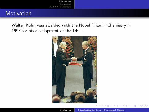
Walter Kohn was awarded with the Nobel Prize in Chemistry in1998 for his development of the DFT.
S. Sharma Introduction to Density Functional Theory

MotivationFormalism
3G DFT + example
Motivation
The following figure shows the number of publications where thephrase DFT appears in the title or abstract (taken from the ISIWeb of Science).
S. Sharma Introduction to Density Functional Theory

MotivationFormalism
3G DFT + example
Motivation
Where can DFT be applied:
1 DFT is presently the most successful (and also the most promising)approach to compute the electronic structure of matter.
2 Its applicability ranges from atoms, molecules and solids to nuclei andquantum and classical fluids.
3 Chemistry: DFT predicts a great variety of molecular properties:molecular structures, vibrational frequencies, atomization energies,ionization energies, electric and magnetic properties, reaction paths, etc
4 The original DFT has been generalized to deal with many differentsituations: spin polarized systems, multicomponent systems, systems atfinite temperatures, superconductors, time-dependent phenomena,Bosons, molecular dynamics ...........
S. Sharma Introduction to Density Functional Theory

MotivationFormalism
3G DFT + example
Elementary QMSolving SE: HFSolving SE: DFT
Elementary quantum mechanics
Schrodinger equation
HΦi(x1,x2...xN ,R1,R2...RM ) = EiΦi(x1,x2, ...xN ,R1,R2...RM )
x ≡ {r, σ}
S. Sharma Introduction to Density Functional Theory

MotivationFormalism
3G DFT + example
Elementary QMSolving SE: HFSolving SE: DFT
Schrodinger equation
Kinetic energy
H = −1
2
N∑
i
∇2i
S. Sharma Introduction to Density Functional Theory
MotivationFormalism
3G DFT + example
Elementary QMSolving SE: HFSolving SE: DFT
Schrodinger equation
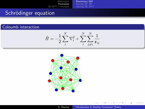
Coloumb interaction
H = −1
2
N∑
i
∇2i +
N∑
i
N∑
j 6=i
1
rij
S. Sharma Introduction to Density Functional Theory

MotivationFormalism
3G DFT + example
Elementary QMSolving SE: HFSolving SE: DFT
Schrodinger equation
Nuclear electron interaction
H = −1
2
N∑
i
∇2i +
N∑
i
N∑
j 6=i
1
rij−
N∑
i
M∑
A
ZA
riA
S. Sharma Introduction to Density Functional Theory
MotivationFormalism
3G DFT + example
Elementary QMSolving SE: HFSolving SE: DFT
Schrodinger equation
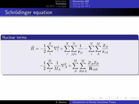
Nuclear terms
H = −1
2
N∑
i
∇2i +
N∑
i
N∑
j 6=i
1
rij−
N∑
i
M∑
A
ZA
riA
−1
2
M∑
i
1
MA∇2
A +M∑
A
M∑
B 6=A
ZAZB
RAB
S. Sharma Introduction to Density Functional Theory

MotivationFormalism
3G DFT + example
Elementary QMSolving SE: HFSolving SE: DFT
Elementary quantum mechanics
Born-Oppenheimer approximation
Due to their masses the nuclei move much slower than the electrons. So wecan consider the electrons as moving in the field of fixed nuclei.
H = −1
2
N∑
i
∇2i +
N∑
i
N∑
j 6=i
1
rij−
N∑
i
M∑
A
ZA
riA= T + VNe + Vee
HΨi(x1,x2...xN ) = EiΨi(x1,x2, ...xN )
S. Sharma Introduction to Density Functional Theory

MotivationFormalism
3G DFT + example
Elementary QMSolving SE: HFSolving SE: DFT
Elementary quantum mechanics
Variational principle
The variational principle states that the energy computed from a guessedwave function Ψ is an upper bound to the true ground-state energy E0. Fullminimization of E with respect to all allowed N-electrons wave functions willgive the true ground state.
E0[Ψ0] = minΨ
E[Ψ] = minΨ
〈Ψ|T + VNe + Vee|Ψ〉
S. Sharma Introduction to Density Functional Theory

MotivationFormalism
3G DFT + example
Elementary QMSolving SE: HFSolving SE: DFT
Elementary quantum mechanics
Energy
E0[Ψ] = 〈Ψ|H|Ψ〉 =
∫
Ψ∗(x)HΨ(x)dx
Wave function : example of two fermions
Pauli exclusion principle results in an antisymmetric wave function
Ψ(x1,x2) = φ1(x1)φ2(x2) − φ1(x2)φ2(x1)
This looks like a determinant∣
∣
∣
∣
φ1(x1) φ2(x1)φ1(x2) φ2(x2)
∣
∣
∣
∣
S. Sharma Introduction to Density Functional Theory

MotivationFormalism
3G DFT + example
Elementary QMSolving SE: HFSolving SE: DFT
Wave function method: Hartree-Fock
The ground state wave function is approximated by a Slaterdeterminant:
ΨHF (x1,x2....xN ) =1√N !
∣
∣
∣
∣
∣
∣
∣
∣
∣
φ1(x1) φ2(x1) · · · φN (x1)φ1(x2) φ2(x2) · · · φN (x2)
......
. . ....
φ1(xN ) φ2(xN ) · · · φN (xN )
∣
∣
∣
∣
∣
∣
∣
∣
∣
The Hartree-Fock approximation is the method whereby theorthogonal orbitals φi are found that minimize the energy. Thevariational principle is used.
EHF = minφHF
E[φHF ]
S. Sharma Introduction to Density Functional Theory

MotivationFormalism
3G DFT + example
Elementary QMSolving SE: HFSolving SE: DFT
Problems with wave function methods
I. Visualization and probing
The conventional wave function approaches use wave function as the centralquantity, since it contains the full information of a system. However, is a verycomplicated quantity that cannot be probed experimentally and that dependson 3N variables, N being the number of electrons.
S. Sharma Introduction to Density Functional Theory

MotivationFormalism
3G DFT + example
Elementary QMSolving SE: HFSolving SE: DFT
Problems with wave function methods
II. Time consuming
The interactions are very difficult to calculate for a realistic system, in factthis is most time consuming part.
Vee =N
∑
i
N∑
j 6=i
1
rij
S. Sharma Introduction to Density Functional Theory

MotivationFormalism
3G DFT + example
Elementary QMSolving SE: HFSolving SE: DFT
Problems with wave function methods
III. Inefficient
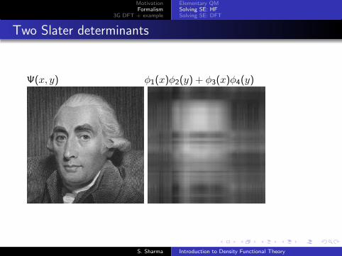
One Slater determinant does a rather bad job for expanding the many-bodywave function.
Ψ(x, y) φ1(x)φ2(y)
S. Sharma Introduction to Density Functional Theory
MotivationFormalism
3G DFT + example
Elementary QMSolving SE: HFSolving SE: DFT
Two Slater determinants
Ψ(x, y) φ1(x)φ2(y) + φ3(x)φ4(y)
S. Sharma Introduction to Density Functional Theory
MotivationFormalism
3G DFT + example
Elementary QMSolving SE: HFSolving SE: DFT
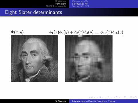
Eight Slater determinants
Ψ(x, y) φ1(x)φ2(y) + φ3(x)φ4(y)......φ15(x)φ16(y)
S. Sharma Introduction to Density Functional Theory

MotivationFormalism
3G DFT + example
Elementary QMSolving SE: HFSolving SE: DFT
Density Functional Theory
Experiments probe density
ρ(r1) =
∫
Ψ∗(x1,x2, .....xN)Ψ(x1,x2, .....xN)dx2....dxN
S. Sharma Introduction to Density Functional Theory

MotivationFormalism
3G DFT + example
Elementary QMSolving SE: HFSolving SE: DFT
Hohenberg-Kohn theorems
I Hohenberg-Kohn theorem
H = T + VNe + Vee
This first theorem states that the VNe is (to within a constant) a uniquefunctional of density (ρ); since, in turn this potential fixes H we see that thefull many particle ground state is a unique functional of density.
S. Sharma Introduction to Density Functional Theory

MotivationFormalism
3G DFT + example
Elementary QMSolving SE: HFSolving SE: DFT
Hohenberg-Kohn theorems
II Hohenberg-Kohn theorem
The second H-K theorem states that the functional that delivers the groundstate energy of the system, delivers the lowest energy if and only if the inputdensity is the true ground state density. This is nothing but the variationalprinciple,but this time with density and not wave function
E0[ρ0] = minρ
E[ρ] = minρ
T [ρ] + ENe[ρ] + Eee[ρ]
S. Sharma Introduction to Density Functional Theory

MotivationFormalism
3G DFT + example
Elementary QMSolving SE: HFSolving SE: DFT
Modern DFT
Energy as a functional of density
E[ρ] = T [ρ] + ENe[ρ] + Eee[ρ]
E[ρ] = T [ρ] + ENe[ρ] + EH [ρ] + Ex[ρ] + Ec[ρ]
S. Sharma Introduction to Density Functional Theory

MotivationFormalism
3G DFT + example
Elementary QMSolving SE: HFSolving SE: DFT
Modern DFT: Kohn-Sham
The system is replaced by a fictitious non-interaction system withsame density as the real system.
Kohn-Sham non-interacting system
E[ρ] = T [ρ] + ENe[ρ] + EH [ρ] + Ex[ρ] + Ec[ρ]
T [ρ] = −1
2〈φi|∇2|φi〉
ENe[ρ] + EH [ρ] = −Z
∫
ρ(r)
rdr − 1
2
∫
ρ(r1)ρ(r2)
r12dr1dr2
Local Density Approximation
Based on the properties of uniform electron gas XC potential is approximatedas:
Exc[ρ] = − 3
4π(3π2)1/3
∫
ρ4/3(r)dr
S. Sharma Introduction to Density Functional Theory

MotivationFormalism
3G DFT + example
Third generation DFT: Exact exchange
Treating exchange term exactly
E[ρ] = T [ρ] + ENe[ρ] + EH [ρ] + Ex[ρ]
Using the Fock integral and its functional derivative the exchange term canbe treated exactly . This method is called EXX or OEP.
S. Sharma, J. K. Dewhurst and C. Ambrosch-DraxlPhys. Rev. Lett. 95 136402 (2005)
S. Sharma Introduction to Density Functional Theory

MotivationFormalism
3G DFT + example
Phase transition in Ce using LDA
140 160 180 200volume (a.u.)3
-0.715
-0.71
-0.705
-0.7
Ene
rgy
(Ha)
S. Sharma Introduction to Density Functional Theory
MotivationFormalism
3G DFT + example
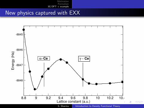
New physics captured with EXX
8.8 9 9.2 9.4 9.6 9.8 10 10.2 10.4Lattice constant (a.u.)
-8848
-8847
-8846
-8845
Ene
rgy
(Ha)
α−Ce γ − Ce
S. Sharma Introduction to Density Functional Theory

MotivationFormalism
3G DFT + example
Many thanks to
1 Funding agency : FWF and Exciting EU network
2 Dr. J. K. Dewhurst
3 D. Rankin and S. Hinchley
4 EXCITING code: http://exciting.sourceforge.net/
S. Sharma Introduction to Density Functional Theory