Introduction to Computer Vision Digitization

World Optics Sensor Signal Digitizer Digital Representation

Introduction to Computer Vision Pre-digitization image

■  What is an image before we digitize it? ●  Continuous range of wavelengths. ●  2-dimensional extent ●  Continuous range of power at each point.

Introduction to Computer Vision Brightness images

■  To simplify, consider only a brightness image: ●  Two-dimensional (continuous range of locations) ●  Continuous range of brightness values.

■  This is equivalent to a two-dimensional function over the plane.

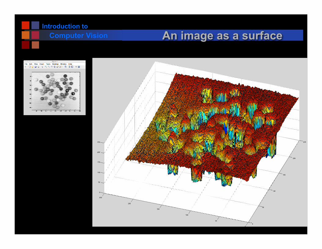
Introduction to Computer Vision An image as a surface

Introduction to Computer Vision An image as a surface

Introduction to Computer Vision Discretization

■  Sampling strategies: ●  Spatial sampling

■  How many pixels? ■  What arrangement of pixels?

●  Brightness sampling ■  How many brightness values? ■  Spacing of brightness values?

●  For video, also the question of time sampling.

Introduction to Computer Vision Projection through a pixel

Central Projection RayCentral Projection Ray

Image irradiance is the average of the scene radiance over the area of the surface intersecting the solid angle!

Digitized 35mm Slide or Film

Introduction to Computer Vision Signal Quantization

■  Goal: determine a mapping from a continuous signal (e.g. analog video signal) to one of K discrete (digital) levels.

I(x,y) = .1583 volts

= ???? Digital value

Introduction to Computer Vision Quantization

■  I(x,y) = continuous signal: 0 ≤ I ≤ M ■  Want to quantize to K values 0,1,....K-1 ■  K usually chosen to be a power of 2:

■  Mapping from input signal to output signal is to be determined. ■  Several types of mappings: uniform, logarithmic, etc.

K: #Levels #Bits 2 1 4 2 8 3 16 4 32 5 64 6 128 7 256 8

Introduction to Computer Vision Choice of K

Original

Linear Ramp

K=2 K=4

K=16 K=32

Introduction to Computer Vision Choice of K

K=2 (each color)

K=4 (each color)

Introduction to Computer Vision Choice of Function: Uniform

■  Uniform sampling divides the signal range [0-M] into K equal-sized intervals.

■  The integers 0,...K-1 are assigned to these intervals. ■  All signal values within an interval are represented by

the associated integer value. ■  Defines a mapping:

Qua

ntiz

atio

n Le

vel

3

M

21

0

K-1

0Signal Value

•••

Introduction to Computer Vision Logarithmic Quantization

■  Signal is log I(x,y). ■  Effect is:

Qua

ntiz

atio

n Le

vel

3

M

21

0

K-1

0Signal Value

•••

■  Detail enhanced in the low signal values at expense of detail in high signal values.

Introduction to Computer Vision Logarithmic Quantization

Original

Logarithmic Quantization

Quantization Curve

Introduction to Computer Vision Color Displays

■  Given a 24-bit color image (8 bits each for R,G,B) ●  Turn on 3 subpixels with power proportional to RGB

values:

http://en.wikipedia.org/wiki/File:Pixel_geometry_01_Pengo.jpg

Introduction to Computer Vision Color Displays

■  Given a 24-bit color image (8 bits each for R,G,B) ●  Turn on 3 subpixels with power proportional to RGB

values:

http://en.wikipedia.org/wiki/File:Pixel_geometry_01_Pengo.jpg

Introduction to Computer Vision “White” text on a color display

http://en.wikipedia.org/wiki/Subpixel_rendering

Introduction to Computer Vision Color selector

Introduction to Computer Vision Constructing a Color LCD Display

■  See movie.

Introduction to Computer Vision Look up tables

■  8 bit image: 256 different values. ●  Simplest way to display: map each number to a gray value:

■  0-> (0.0, 0.0, 0.0) ■  1->(0.0039, 0.0039, 0.0039) or (1,1,1) ■  2->(0.0078, 0.0078, 0.0078) or (2,2,2) ■  ... ■  255-> (1.0, 1.0, 1.0) or (255,255,255)

●  This is called a grayscale image.

Introduction to Computer Vision Lookup tables

im (24 bits) “true color”

im8 (8 bits) gray color look up table

Introduction to Computer Vision Non-gray look up tables

■  We can also use other mappings: ●  0->(17, 25, 89) ●  1-> (45, 32, 200) ●  ... ●  255-> (233,1,4)

●  These are called look up tables.

Introduction to Computer Vision More look up tables.

Introduction to Computer Vision Fun with matlab

Introduction to Computer Vision Enhancing images

■  What can we do to “enhance” an image after it has already been digitized? ●  We can make the information that is there easier to

visualize. ●  We can guess at data that is not there, but we cannot

be sure, in general.

Introduction to Computer Vision Can we “enhance” an image after digitization?

Introduction to Computer Vision Brightness Equalization

■  Two methods: ●  Change the data (histogram equalization) ●  Use a look up table (brightness or color remapping)

Introduction to Computer Vision Histogram Equalization

Introduction to Computer Vision Histogram Equalization

Introduction to Computer Vision Histogram Equalization

Introduction to Computer Vision Brightness Equalization

■  Two methods: ●  Change the data (histogram equalization). ●  Use a look up table (brightness equalization).

Make this value black

Make this value white

Introduction to Computer Vision Look up tables

Map lowest value in image to black, highest value to white. ■  0 -> (0, 0, 0) ■  1 -> (0, 0, 0) ■  2 -> (0, 0, 0) ■  3 -> (0 , 0, 0) ■  ... ■  130-> (0,0,0) ■  131-> (.01, .01, .01) ■  132-> (.02,.02,.02) ■  ... ■  229->(1,1,1) ■  230->(1,1,1) ■  ... ■  255 -> (1, 1, 1)

Introduction to Computer Vision Brightness Equalization

Introduction to Computer Vision Mixed Pixel Problem

Introduction to Computer Vision Mixed Pixel Problem

Introduction to Computer Vision Pattern Recognition

■  Typical recognition problems: ●  Recognize letters and words ●  Recognize people ●  Recognize classes of objects ●  Recognize places

Introduction to Computer Vision Recognizing Text

Introduction to Computer Vision Recognizing People

Introduction to Computer Vision Classes of objects

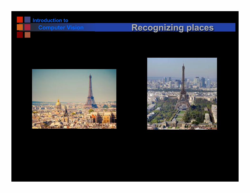
Introduction to Computer Vision Recognizing places

Introduction to Computer Vision Recognizing Handwritten Digits

Introduction to Computer Vision Supervised Learning

■  Supervised learning: ●  Formalization of the idea of learning from examples.

■  2 elements: ●  Training data ●  Test data

■  Training data: ●  Data in which the class has been identified.

■  Example: This is a “three”.

■  Test data: ●  Data which the algorithm is supposed to identify. ●  What is this?

Introduction to Computer Vision Supervised learning

■  Formally: ●  n training data pairs:

x’s are “observations” y’s are the class labels

●  m test data samples: