introduction to computational linguistics and natural...
TRANSCRIPT

Introduction to Computational Linguisticsand Natural Language Processing
Mark Johnson
Department of ComputingMacquarie University
2014 Machine Learning Summer School
Updated slides available fromhttp://web.science.mq.edu.au/˜mjohnson/
1/162
Outline
Overview of computational linguistics and natural language processing
Key ideas in NLP and CL
Grammars and parsing
Conclusion and future directions
Non-parametric Bayesian extensions to grammars
2/162
Natural language processing and computational linguistics
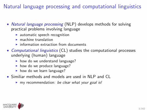
• Natural language processing (NLP) develops methods for solvingpractical problems involving language
I automatic speech recognitionI machine translationI information extraction from documents
• Computational linguistics (CL) studies the computational processesunderlying (human) language
I how do we understand language?I how do we produce language?I how do we learn language?
• Similiar methods and models are used in NLP and CLI my recommendation: be clear what your goal is!
3/162

A brief history of CL and NLP
• Computational linguistics goes back to the dawn of computer scienceI syntactic parsing and machine translation started in the 1950s
• Until the 1990s, computational linguistics was closely connected tolinguistics
I linguists write grammars, computational linguists implement them
• The “statistical revolution” in the 1990s:I techniques developed in neighbouring fields work better
– hidden Markov models produce better speech recognisers– bag-of-words methods like tf-idf produce better information retrieval
systems
⇒ NLP and CL adopted probabilistic models
• NLP and CL today:I oriented towards machine learning rather than linguisticsI NLP applications-oriented, driven by large internet companies
4/162

Outline
Overview of computational linguistics and natural language processingLinguistic levels of descriptionSurvey of NLP applications
Key ideas in NLP and CL
Grammars and parsing
Conclusion and future directions
Non-parametric Bayesian extensions to grammars
5/162

Phonetics and phonology
• Phonetics studies the sounds of a languageI E.g., [t] and [d] differ in voice onset timeI E.g., English aspirates stop consonants in certain positions
(e.g., [thop] vs. [stop])
• Phonology studies the distributional properties of these soundsI E.g., the English noun plural is [s] following unvoiced segments and [z]
following voiced segmentsI E.g., English speakers pronounce /t/ differently (e.g., in water)
6/162

Morphology
• Morphology studies the structure of wordsI E.g., re+structur+ing, un+remark+able
• Derivational morphology exhibits hierarchical structure
• Example: re+vital+ize+ationNoun
Verb
Verb
re+
Verb
Adjective
vital
Verb
+ize
Noun
+ation
• The suffix usually determines the syntactic category of the derived word
7/162

Syntax
• Syntax studies the ways words combine to form phrases and sentences
Sentence
NounPhrase
Determiner
the
Noun
cat
VerbPhrase
Verb
chased
NounPhrase
Determiner
the
Noun
dog
• Syntactic parsing helps identify who did what to whom, a key step inunderstanding a sentence
8/162

Semantics and pragmatics
• Semantics studies the meaning of words, phrases and sentencesI E.g., I ate the oysters in/for an hour.I E.g., Who do you want to talk to ∅/him?
• Pragmatics studies how we use language to do things in the worldI E.g., Can you pass the salt?I E.g., in a letter of recommendation:
Sam is punctual and extremely well-groomed.
9/162

The lexicon
• A language has a lexicon, which lists for eachmorpheme
I how it is pronounced (phonology),I its distributional properties (morphology and
syntax),I what it means (semantics), andI its discourse properties (pragmatics)
• The lexicon interacts with all levels oflinguistic representation
Morphology
Syntax
Semantics
Pragmatics
Meaning
Phonology
Sound
Lex
icon
10/162

Linguistic levels on one slide
• Phonology studies the distributional patterns of soundsI E.g., cats vs dogs
• Morphology studies the structure of wordsI E.g., re+vital+ise
• Syntax studies how words combine to form phrases and sentencesI E.g., Flying planes can be dangerous
• Semantics studies how meaning is associated with languageI E.g., I sprayed the paint onto the wall/I sprayed the wall with paint
• Pragmatics studies how language is used to do thingsI E.g., Can you pass the salt?
• The lexicon stores phonological, morphological, syntactic, semantic andpragmatic information about morphemes and words
11/162

Outline
Overview of computational linguistics and natural language processingLinguistic levels of descriptionSurvey of NLP applications
Key ideas in NLP and CL
Grammars and parsing
Conclusion and future directions
Non-parametric Bayesian extensions to grammars
12/162

What’s driving NLP and CL research?
• Tools for managing the “information explosion”I extracting information from and managing large text document collectionsI NLP is often free “icing on the cake” to sell more ads;
e.g., speech recognition, machine translation, document clustering(news), etc.
• Mobile and portable computingI keyword search / document retrieval don’t work well on very small devicesI we want to be able to talk to our computers (speech recognition)
and have them say something intelligent back (NL generation)
• The intelligence agencies
• The old Artificial Intelligence (AI) dreamI language is the richest window into the mind
13/162

Automatic speech recognition
• Input: an acoustic waveform a
• Output: a text transcript t(a) of a
• Challenges for Automatic Speech Recognition (ASR):I speaker and pronunciation variability
the same text can be pronounced in many different waysI homophones and near homophones:
e.g. recognize speech vs. wreck a nice beach
14/162

Machine translation
• Input: a sentence (usually text) f in the source language
• Output: a sentence e in the target language
• Challenges for Machine Translation:I the best translation of a word or phrase depends on the contextI the order of words and phrases varies from language to languageI there’s often no single “correct translation”
15/162

The inspiration for statistical machine translation
Also knowing nothing official about, but having guessed andinferred considerable about, powerful new mechanized methods incryptography — methods which I believe succeed even when onedoes not know what language has been coded — one naturallywonders if the problem of translation could conceivably be treatedas a problem in cryptography.
When I look at an article in Russian, I say “This is really written inEnglish, but it has been coded in some strange symbols. I will nowproceed to decode.”
Warren Weaver – 1947
16/162

Topic modelling
• Topic models cluster documents onsame topic
I unsupervised (i.e., topics aren’tgiven in training data)
• Important for document analysis andinformation extraction
I Example: clustering news storiesfor information retrieval
I Example: tracking evolution of aresearch topic over time
17/162

Example input to a topic model (NIPS corpus)
Annotating an unlabeled dataset is one of the bottlenecks in using supervised learning tobuild good predictive models. Getting a dataset labeled by experts can be expensive andtime consuming. With the advent of crowdsourcing services . . .
The task of recovering intrinsic images is to separate a given input image into itsmaterial-dependent properties, known as reflectance or albedo, and its light-dependentproperties, such as shading, shadows, specular highlights, . . .
In each trial of a standard visual short-term memory experiment, subjects are firstpresented with a display containing multiple items with simple features (e.g. coloredsquares) for a brief duration and then, after a delay interval, their memory for . . .
Many studies have uncovered evidence that visual cortex contains specialized regionsinvolved in processing faces but not other object classes. Recent electrophysiology studiesof cells in several of these specialized regions revealed that at least some . . .
18/162

Example (cont): ignore function words
Annotating an unlabeled dataset is one of the bottlenecks in using supervised learning tobuild good predictive models. Getting a dataset labeled by experts can be expensive andtime consuming. With the advent of crowdsourcing services . . .
The task of recovering intrinsic images is to separate a given input image into itsmaterial-dependent properties, known as reflectance or albedo, and its light-dependentproperties, such as shading, shadows, specular highlights, . . .
In each trial of a standard visual short-term memory experiment, subjects are firstpresented with a display containing multiple items with simple features (e.g. coloredsquares) for a brief duration and then, after a delay interval, their memory for . . .
Many studies have uncovered evidence that visual cortex contains specialized regionsinvolved in processing faces but not other object classes. Recent electrophysiology studiesof cells in several of these specialized regions revealed that at least some . . .
19/162
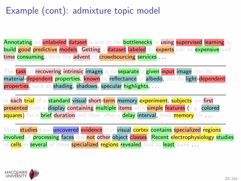
Example (cont): admixture topic model
Annotating an unlabeled dataset is one of the bottlenecks in using supervised learning tobuild good predictive models. Getting a dataset labeled by experts can be expensive andtime consuming. With the advent of crowdsourcing services . . .
The task of recovering intrinsic images is to separate a given input image into itsmaterial-dependent properties, known as reflectance or albedo, and its light-dependentproperties, such as shading, shadows, specular highlights, . . .
In each trial of a standard visual short-term memory experiment, subjects are firstpresented with a display containing multiple items with simple features (e.g. coloredsquares) for a brief duration and then, after a delay interval, their memory for . . .
Many studies have uncovered evidence that visual cortex contains specialized regionsinvolved in processing faces but not other object classes. Recent electrophysiology studiesof cells in several of these specialized regions revealed that at least some . . .
20/162

Phrase structure and dependency parses
S
NP
D
the
N
cat
VP
V
chased
NP
D
a
N
dog the cat chased a dog
sbjdobj
det det
• A phrase structure parse represents phrases as nodes in a tree
• A dependency parse represents dependencies between words
• Phrase structure and dependency parses are approximatelyinter-translatable:
I Dependency parses can be translated to phrase structure parsesI If every phrase in a phrase structure parse has a head word, then phrase
structure parses can be translated to dependency parses
21/162

Syntactic structures of real sentences
S
NP-SBJ
DT
The
JJ
new
NNS
options
VP
VBP
carry
PRT
RP
out
NP
NP
NN
part
PP
IN
of
NP
NP
DT
an
NN
agreement
SBAR
WHNP-12
IN
that
S
NP-SBJ-1
DT
the
NN
pension
NN
fund
,
,
S-ADV
NP-SBJ
-NONE-
*-1
PP-PRD
IN
under
NP
NN
pressure
S
NP-SBJ
-NONE-
*
VP
VP
TO
to
VP
VB
relax
NP
PRP$
its
JJ
strict
NN
participation
NNS
rules
CC
and
VP
TO
to
VP
VB
provide
NP
JJR
more
NN
investment
NNS
options
,
,
VP
VBN
reached
NP
-NONE-
*T*-12
PP
IN
with
NP
DT
the
NNP
SEC
PP-TMP
IN
in
NP
NNP
December
.
.
• State-of-the-art parsers have accuracies of over 90%• Dependency parsers can parse thousands of sentences a second
22/162

Advantages of probabilistic parsing
• In the GofAI approach to syntactic parsing:I a hand-written grammar defines the grammatical (i.e., well-formed) parsesI given a sentence, the parser returns the set of grammatical parses for that
sentence⇒ unable to distinguish more likely from less likely parses⇒ hard to ensure robustness (i.e., that every sentence gets a parse)
• In a probabilistic parser:I the grammar generates all possible parse trees for all possible strings
(roughly)I use probabilities to identify plausible syntactic parses
• Probabilistic syntactic models usually encode:I the probabilities of syntactic constructionsI the probabilities of lexical dependencies
e.g., how likely is pizza as direct object of eat?
23/162

Named entity recognition and linking
• Named entity recognition finds all “mentions” referring to an entity in adocument
Example: Tony Abbott︸ ︷︷ ︸person
bought 300︸︷︷︸number
shares in Acme Corp︸ ︷︷ ︸corporation
in 2006︸︷︷︸date
• Noun phrase coreference tracks mentions to entities within or acrossdocuments
Example: Julia Gillard met the president of Indonesia yesterday. Ms.Gillard told him that she . . .
• Entity linking maps entities to database entries
Example: Tony Abbott︸ ︷︷ ︸/m/xw2135
bought 300︸︷︷︸number
shares in Acme Corp︸ ︷︷ ︸/m/yzw9w
in 2006︸︷︷︸date
24/162

Relation extraction
• Relation extraction mines texts to find relationships between namedentities, i.e., “who did what to whom (when)?”
The new Governor General, Peter Cosgrove, visited Buckingham Palaceyesterday.
Has-rolePerson Role
Peter Cosgrove Governor General of Australia
Offical-visitVisitor Organisation
Peter Cosgrove Queen of England
• The syntactic parse provides useful features for relation extraction
• Text mining bio-medical literature is a major application
25/162

Syntactic parsing for relation extraction
The Governor General, Peter Cosgrove, visited Buckingham Palace
sbjdobj
det
nnappos
nn nn
• The syntactic path in a dependency parse is a useful feature in relationextraction
Xappos−→ Y ⇒ has-role(Y ,X )
Xsbj←− visited
dobj−→Y ⇒ official-visit(X ,Y )
26/162

Google’s Knowledge Graph
• Goal: move beyond keywordsearch document retrieval todirectly answer user queries
⇒ easier for mobile device users
• Google’s Knowledge Graph:I built on top of FreeBaseI entries are synthesised from
Wikipedia, news stories, etc.I manually curated (?)
27/162

FreeBase: an open (?) knowledge base
• An entity-relationship databaseon top of a graph triple store
• Data mined from Wikipedia,ChefMoz, NNDB, FMD,MusicBrainz, etc.
• 44 million topics (entities),2 billion facts,25GB compressed dump
• Created by Metaweb, which wasacquired by Google
28/162

Distant supervision for relation extraction
• Ideal labelled data for relation extraction: large text corpus annotatedwith entities and relations
I expensive to produce, especially for a lot of relations!
• Distant supervision assumption: if two or more entities that appear inthe same sentence also appear in the same database relation, thenprobably the sentence expresses the relation
I assumes entity tuples are sparse
• With the distant supervision assumption, we obtain relation extractiontraining data by:
I taking a large text corpus (e.g., 10 years of news articles)I running a named entity linker on the corpusI looking up the entity tuples that appear in the same sentence in the large
knowledge base (e.g., FreeBase)
29/162

Opinion mining and sentiment analysis
• Used to analyse e.g., social media (Web 2.0)
• Typical goals: given a corpus of messages:I classify each message along a subjective–objective scaleI identify the message polarity (e.g., on dislike–like scale)
• Training opinion mining and sentiment analysis models:I in some domains, supervised learning with simple keyword-based features
works wellI but in other domains it’s necessary to model syntactic structure as well
– E.g., I doubt she had a very good experience . . .
• Opinion mining can be combined with:I topic modelling to cluster messages with similar opinionsI multi-document summarisation to summarise results
30/162

Why do statistical models work so well?
• Statistical models can be trained from large datasetsI large document collections are available or can be constructedI machine learning methods can automatically adjust a model so it
performs well on the data it will be used on
• Probabilistic models can integrate disparate and potentially conflictingevidence
I standard linguistic methods make hard categorical classificationsI the weighted features used in probabilistic models can weigh conflicting
information from diverse sources
• Statistical models can rank alternative possible analysesI in NLP, the number of possible analyses is often astronomicalI a statistical model provides a principled way of selecting the most
probable analysis
31/162
Outline
Overview of computational linguistics and natural language processing
Key ideas in NLP and CL
Grammars and parsing
Conclusion and future directions
Non-parametric Bayesian extensions to grammars
32/162
Why is NLP difficult?
• Abstractly, most NLP applications can be viewed as prediction problems⇒ should be able to solve them with Machine Learning
• The label set is often the set of all possible sentencesI infinite (or at least astronomically large)I constrained in ways we don’t fully understand
• Training data for supervised learning is often not available⇒ techniques for training from available data
• Algorithmic challengesI vocabulary can be large (e.g., 50K words)I data sets are often large (GB or TB)
33/162

Outline
Overview of computational linguistics and natural language processing
Key ideas in NLP and CLThe noisy channel modelLanguage modelsSequence labelling modelsExpectation Maximisation (EM)
Grammars and parsing
Conclusion and future directions
Non-parametric Bayesian extensions to grammars
34/162
Motivation for the noisy channel model
• Speech recognition and machine translation models as predictionproblems:
I speech recognition: given an acoustic string, predict the textI translation: given a foreign source language sentence, predict its target
language translation
• The “natural” training data for these tasks is relatively rare/expensive:I speech recognition: acoustic signals labelled with text transcriptsI translation: (source language sentence,target language translation) pairs
• The noisy channel model lets us leverage monolingual text data inoutput language
I large amounts of such text are cheaply available
35/162

The noisy channel model
• The noisy channel model is a commonstructure for generative models
I the source y is a hidden variable generatedby P(y)
I the output x is a visible variable generatedfrom y by P(y | x)
• Given output x , find most likely source y(x)
y(x) = argmax P(y | x)
• Bayes rule: P(y | x) =P(x | y) P(y)
P(x)
• Since output x is fixed:
y(x) = argmaxy
P(x | y) P(y)
Source model P(y)
Source y
Channel model P(x | y)
Output x
36/162

The noisy channel model in speech recognition
• Input: acoustic signal a
• Output: most likely text t(a), where:
t(a) = argmaxt
P(t | a)
= argmaxt
P(a | t) P(t), where:
I P(a | t) is an acoustic model, andI P(t) is an language model
• The acoustic model uses pronouncing dictionaries to decompose thesentence t into sequences of phonemes, and map each phoneme to aportion of the acoustic signal a
• The language model is responsible for distinguishing more likelysentences from less likely sentences in the output text,e.g., distinguishing recognise speech vs. wreck a nice beach
37/162

The noisy channel model in machine translation
• Input: target language sentence f
• Output: most likely source language sentence e(f ), where:
e(f ) = argmaxe
P(e | f )
= argmaxe
P(f | e) P(e), where:
I P(f | e) is a translation model, andI P(e) is an language model
• The translation model calculates P(f | e) as a product of twosubmodels:
I a word or a phrase translation modelI a distortion model, which accounts for the word and phrase reorderings
between source and target language
• The language model is responsible for distinguishing more fluentsentences from less fluent sentences in the target language,e.g., distinguishing Sasha will the car lead vs. Sasha will drive the car
38/162

Outline
Overview of computational linguistics and natural language processing
Key ideas in NLP and CLThe noisy channel modelLanguage modelsSequence labelling modelsExpectation Maximisation (EM)
Grammars and parsing
Conclusion and future directions
Non-parametric Bayesian extensions to grammars
39/162
The role of language models
• A language model estimates the probability P(w) that a string of wordsw is a sentence
I useful in tasks such as speech recognition and machine translation thatinvolve predicting entire sentences
• Language models provide a way of leveraging large amounts of text(e.g., from the web)
• Primary challenge in language modelling: infinite number of possiblesentences
⇒ Factorise P(w) into a product of submodelsI we’ll look at n-gram sequence models hereI but syntax-based language models are also used, especially in machine
translation
40/162

n-gram language models
• Goal: estimate P(w), where w = (w1, . . . ,wm) is a sequence of words
• n-gram models decompose P(w) into product of conditionaldistributions
P(w) = P(w1)P(w2 | w1)P(w3 | w1,w2) . . .P(wm | w1, . . . ,wm−1)
E.g., P(wreck a nice beach) = P(wreck) P(a | wreck) P(nice | wreck a)
P(beach | wreck a nice)
• n-gram assumption: no dependencies span more than n words, i.e.,
P(wi | w1, . . . ,wi−1) ≈ P(wi | wi−n, . . . ,wi−1)
E.g., A bigram model is an n-gram model where n = 2:
P(wreck a nice beach) ≈ P(wreck) P(a | wreck) P(nice | a)
P(beach | nice)
41/162
n-gram language models as Markov models and Bayes nets
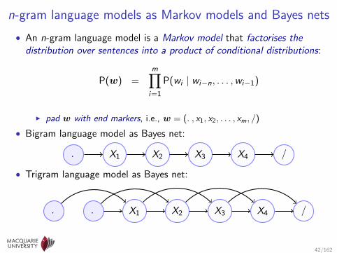
• An n-gram language model is a Markov model that factorises thedistribution over sentences into a product of conditional distributions:
P(w) =m∏i=1
P(wi | wi−n, . . . ,wi−1)
I pad w with end markers, i.e., w = (., x1, x2, . . . , xm, /)
• Bigram language model as Bayes net:
. X1 X2 X3 X4 /
• Trigram language model as Bayes net:
. . X1 X2 X3 X4 /
42/162

The conditional word models in n-gram models
• An n-gram model factorises P(w) into a product of conditional models,each of the form:
P(xn | x1, . . . , xn−1)
• The performance of an n-gram model depends greatly on exactly howthese conditional models are defined
I huge amount of work on this
• Deep learning methods for estimating these conditional distributionscurrently produce state-of-the-art language models
43/162

Outline
Overview of computational linguistics and natural language processing
Key ideas in NLP and CLThe noisy channel modelLanguage modelsSequence labelling modelsExpectation Maximisation (EM)
Grammars and parsing
Conclusion and future directions
Non-parametric Bayesian extensions to grammars
44/162

What is sequence labelling?
• A sequence labelling problem is one where:I the input consists of a sequence X = (X1, . . . ,Xn), andI the output consists of a sequence Y = (Y1, . . . ,Yn) of labels, where:I Yi is the label for element Xi
• Example: Part-of-speech tagging(YX
)=
(Verb, Determiner, Noun
spread, the, butter
)• Example: Spelling correction(
YX
)=
(write, a, bookrite, a, buk
)
45/162

Named entity extraction with IOB labels
• Named entity recognition and classification (NER) involves finding thenamed entities in a text and identifying what type of entity they are(e.g., person, location, corporation, dates, etc.)
• NER can be formulated as a sequence labelling problem
• Inside-Outside-Begin (IOB) labelling scheme indicates the beginning andspan of each named entity
B-ORG I-ORG O O O B-LOC I-LOC I-LOC OMacquarie University is located in New South Wales .
• The IOB labelling scheme lets us identify adjacent named entities
B-LOC I-LOC I-LOC B-LOC I-LOC O B-LOC O . . .New South Wales Northern Territory and Queensland are . . .
• This technology can extract information from:I news storiesI financial reportsI classified ads
46/162

Other applications of sequence labelling
• Speech transcription as a sequence labelling taskI The input X = (X1, . . . ,Xn) is a sequence of acoustic frames Xi , where
Xi is a set of features extracted from a 50msec window of the speechsignal
I The output Y is a sequence of words (the transcript of the speech signal)
• Financial applications of sequence labellingI identifying trends in price movements
• Biological applications of sequence labellingI gene-finding in DNA or RNA sequences
47/162

A first (bad) approach to sequence labelling
• Idea: train a supervised classifier to predict entire label sequence at once
B-ORG I-ORG O O O B-LOC I-LOC I-LOC OMacquarie University is located in New South Wales .
• Problem: the number of possible label sequences grows exponentiallywith the length of the sequence
I with binary labels, there are 2n different label sequences of a sequence oflength n (232 = 4 billion)
⇒ most labels won’t be observed even in very large training data sets
• This approach fails because it has massive sparse data problems
48/162

A better approach to sequence labelling
• Idea: train a supervised classifier to predict the label of one word at atime
B-LOC I-LOC O O O O O B-LOC OWestern Australia is the largest state in Australia .
• Avoids sparse data problems in label space
• As well as current word, classifiers can use previous and following wordsas features
• But this approach can produce inconsistent label sequences
O B-LOC I-LOC I-ORG O O O OThe New York Times is a newspaper .
⇒ Track dependencies between adjacent labelsI “chicken-and-egg” problem that Hidden Markov Models and Conditional
Random Fields solve!
49/162
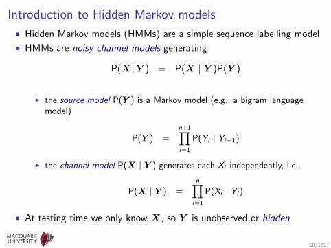
Introduction to Hidden Markov models
• Hidden Markov models (HMMs) are a simple sequence labelling model
• HMMs are noisy channel models generating
P(X,Y ) = P(X | Y )P(Y )
I the source model P(Y ) is a Markov model (e.g., a bigram languagemodel)
P(Y ) =n+1∏i=1
P(Yi | Yi−1)
I the channel model P(X | Y ) generates each Xi independently, i.e.,
P(X | Y ) =n∏
i=1
P(Xi | Yi )
• At testing time we only know X, so Y is unobserved or hidden
50/162

Terminology in Hidden Markov Models
• Hidden Markov models (HMMs) generate pairs of sequences (x,y)
• The sequence x is called:I the input sequence, orI the observations, orI the visible data
because x is given when an HMM is used for sequence labelling
• The sequence y is called:I the label sequence, orI the tag sequence, orI the hidden data
because y is unknown when an HMM is used for sequence labelling
• A y ∈ Y is sometimes called a hidden state because an HMM can beviewed as a stochastic automaton
I each different y ∈ Y is a state in the automatonI the x are emissions from the automaton
51/162

Hidden Markov models
• A Hidden Markov Model (HMM) defines a joint distribution P(X,Y )over:
I item sequences X = (X1, . . . ,Xn) andI label sequences Y = (Y0 = .,Y1, . . . ,Yn,Yn+1 = /):
P(X,Y ) =
(n∏
i=1
P(Yi | Yi−1) P(Xi | Yi )
)P(Yn+1 | Yn)
• HMMs can be expressed as Bayes nets, and standard message-passinginference algorithms work well with HMMs
. Y1 Y2 Y3 Y4 /
X1 X2 X3 X4
52/162

Conditional random fields
• Conditional Random Fields (CRFs) are the Markov Random Fieldgeneralisation of HMMs.
P(X,Y ) =1
Z
(n∏
i=1
θYi−1,YiψYi ,Xi
)θYn,Yn+1
• CRFs are usually used to define conditional distributions P(Y |X) overlabel sequences Y given observed sequences X
• CRFs can be expressed using the undirected MRF graphical models
. Y1 Y2 Y3 Y4 /
X1 X2 X3 X4
53/162
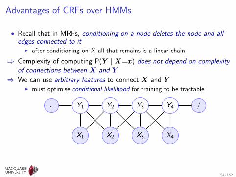
Advantages of CRFs over HMMs
• Recall that in MRFs, conditioning on a node deletes the node and alledges connected to it
I after conditioning on X all that remains is a linear chain
⇒ Complexity of computing P(Y |X=x) does not depend on complexityof connections between X and Y
⇒ We can use arbitrary features to connect X and YI must optimise conditional likelihood for training to be tractable
. Y1 Y2 Y3 Y4 /
X1 X2 X3 X4
54/162

Outline
Overview of computational linguistics and natural language processing
Key ideas in NLP and CLThe noisy channel modelLanguage modelsSequence labelling modelsExpectation Maximisation (EM)
Grammars and parsing
Conclusion and future directions
Non-parametric Bayesian extensions to grammars
55/162

Ideal training data for acoustic models
• The acoustic model P(a | t) in a speech recogniser predicts the acousticwaveform a given a text transcript t
• Ideal training data for an acoustic model would:I segment the acoustic waveform into phonesI map the phones to words in the text
• Manually segmenting and labelling speech is very expensive!
• Expectation Maximisation lets us induce this information from cheapsentence level transcripts
56/162

Ideal training data for the translation model
• The translation model P(f | e) in a MT system:I predicts the translation of each word or phrase, andI predicts the reordering or words and phrases
• Ideal training data would align words and phrases in the source andtarget language sentences
Sasha wants to buy a car
Sasha will einen Wagen kaufen
• Manually aligning words and phrases is very expensive!
• Expectation Maximisation lets us induce this information from cheapsentence aligned translations
57/162

What Expectation Maximisation does
• Expectation Maximisation (and related techniques such as Gibbssampling and Variational Bayes) are “recipies” for generalisingmaximum likelihood supervised learning methods to unsupervisedlearning problems
I they are techniques for hidden variable imputation
• Intuitive idea behind the EM algorithm:I if we had a good acoustic model/translation model,
we could use it to compute the phoneme labelling/word alignment
• Intuitive description of the EM algorithm:
guess an initial model somehow:repeat until converged:
use current model to label the datalearn a new model from the labelled data
• Amazingly, this provably converges under very general conditions, and
• it converges to a local maximum of the likelihood
58/162

Forced alignment for training speech recognisers
• Speech recogniser training typically uses forced alignment to produce aphone labelling of the training data
• Inputs to forced alignment:I a speech corpus with sentence-level transcriptsI a pronouncing dictionary, mapping words to their possible phone
sequencesI an acoustic model mapping phones to waveforms trained on a small
amount of data
• Forced alignment procedure (a version of EM)
repeat until converged:for each sentence s in the training data:
use pronouncing dictionary to find all possible phone sequences for suse current acoustic model to compute probability
of each possible alignment of each phone sequencekeep most likely phone alignments for s
retrain acoustic model based on most likely phone alignments
59/162

Mathematical description of EM• Input: data x and a model P(x , z , θ) where finding the “visible data”
MLE θ would be easy if we knew x and z :
θ = argmaxθ
log Pθ(x , z)
• The “hidden data” MLEθ (which EM approximates) is:
θ = argmaxθ
log Pθ(x) = argmaxθ
log∑z
Pθ(x , z)
• The EM algorithm:initialise θ(0) somehow (e.g., randomly)
for t = 1, 2, . . . until convergence:E-step: set Q(t)(z) = Pθ(t−1) (x , z)M-step: set θ(t) = argmaxθ
∑z Q
(t)(z) log Pθ(x , z)
• θ(t) converges to a local maximum of the hidden data likelihoodI the Q(z) distributions impute values for the hidden variable zI in practice we summarise Q(z) with expected values of the sufficient
statistics for θ
60/162

EM versus directly optimising log likelihood
• It’s possible to directly optimise the “hidden data” log likelihood with agradient-based approach (e.g., SGD, L-BFGS):
θ = argmax
θlog Pθ(x) = argmax
θlog∑z
Pθ(x , z)
• The log likelihood is typically not convex ⇒ local maxima
• If the model is in the exponential family (most NLP models are), thederivatives of the log likelihood are the same expectations as requiredfor EM
⇒ both EM and direct optimisation are equally hard to program
• EM has no adjustable parameters, while SGD and L-BFGS haveadjustable parameters (e.g., step size)
• I don’t know of any systematic study, but in my experience:I EM starts faster ⇒ if you’re only going to do a few iterations, use EMI after many iterations, L-BFGS converges faster (quadratically)
61/162

A word alignment matrix for sentence translation pair
They have full access to working documents
Ils
ont
acces
a
tous
le
documents
de
travail
• Can we use this to learn the probability P(f | e) = θf ,e of English worde translating to French word f ?
62/162
Learning P(f | e) from a word-aligned corpus
• A word alignment a pairs each Frenchword fk with its English translationword eak
I an English word may be aligned withseveral French words
I ♦ generates French words with noEnglish translation
• Let P(f | e) = θf ,e . The MLE θ is:
θf ,e =nf ,e(a)
n·,e(a), where:
nf ,e(a) = number of times f aligns to e
n·,e(a) =∑f
nf ,e(a)
= number of times e aligns to anything
Ils
ont
acces
a
tous
le
de
travail
They
have
♦0
1
2
3
4
5
6
7
full
access
to
working
documents documents
faePosition
a = (1, 2, 4, 5, 3, 0, 7, 0, 6)
63/162

Sentence-aligned parallel corpus (Canadian Hansards)
• English: eprovincial officials are consulted through conference calls and negotiateddebriefings .they have full access to working documents .consultations have also taken place with groups representing specificsectors of the Canadian economy , including culture , energy , mining ,telecommunications and agrifood .
• French: fles fonctionnaires provinciaux sont consultes par appels conference etcomptes rendus .ils ont acces a tous les documents de travail .les consultations ont aussi eu lieu avec de les groupes representant deles secteurs precis de le economie canadienne , y compris la culture , leenergie , les mines , les telecommunications et le agro - alimentaire .
• Word alignments a are not included!
64/162

Learning word translations θ and alignments a with EM
• It is easy to learn translation probabilities θ from word-aligned data(e,f ,a)
• But the available data is only sentence aligned (e,f)I a is a hidden variable
• This is a perfect problem for Expectation Maximisation!I simultaneously learn translation probabilities θ and word alignments a
• It turns out that a very stupid probabilistic model of Pθ(f ,a | e) (IBMModel 1) plus EM produces good word alignments a!
I IBM developed more sophisticated models, up to IBM Model 5
65/162

The IBM Model 1 generative story
• IBM Model 1 defines Pθ(A,F | E)I θf ,e is probability of generating French word f when aligned to English
word e
• Each French word Fk , k = 1, . . . , n is generated independentlyconditional on English words e = (e1, . . . , em)
• To generate French word Fk given English words e:I generate an alignment Ak ∈ 1, . . . ,m for Fk uniformly at randomI generate French word Fk from θeak
Fk
Ak
θeEj
nm E
66/162
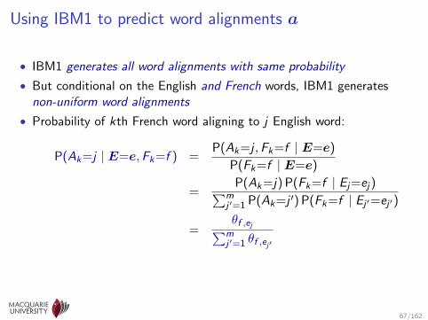
Using IBM1 to predict word alignments a
• IBM1 generates all word alignments with same probability
• But conditional on the English and French words, IBM1 generatesnon-uniform word alignments
• Probability of kth French word aligning to j English word:
P(Ak=j | E=e,Fk=f ) =P(Ak=j ,Fk=f | E=e)
P(Fk=f | E=e)
=P(Ak=j) P(Fk=f | Ej=ej)∑m
j ′=1 P(Ak=j ′) P(Fk=f | Ej ′=ej ′)
=θf ,ej∑m
j ′=1 θf ,ej′
67/162

Example alignment calculation• English and French strings:
e = (the,morning) f = (le,matin)
• English word to French word translation probabilities:
θ =
the a morning evening
le 0.7 0.1 0.2 0.2un 0.1 0.7 0.2 0.2
matin 0.1 0.1 0.3 0.3soir 0.1 0.1 0.3 0.3
• Alignment probability calculation:
P(A1=1 | E=(the,morning),F1=le) =θle,the
θle,the + θle,morning
= 0.7/(0.7 + 0.2)
P(A2=2 | E=(the,morning),F2=matin) =θmatin,morning
θmatin,the + θmatin,morning
= 0.3/(0.1 + 0.3)
68/162
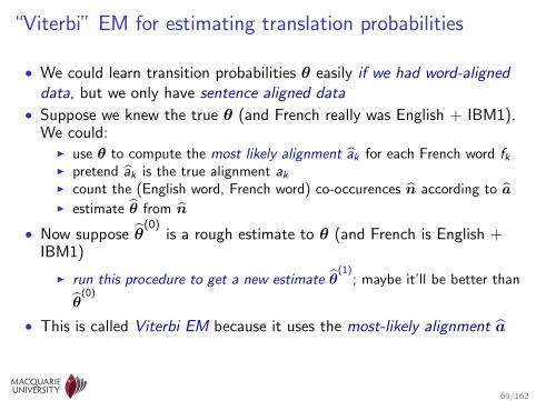
“Viterbi” EM for estimating translation probabilities
• We could learn transition probabilities θ easily if we had word-aligneddata, but we only have sentence aligned data
• Suppose we knew the true θ (and French really was English + IBM1).We could:
I use θ to compute the most likely alignment ak for each French word fkI pretend ak is the true alignment akI count the (English word, French word) co-occurences n according to aI estimate θ from n
• Now suppose θ(0)
is a rough estimate to θ (and French is English +IBM1)
I run this procedure to get a new estimate θ(1)
; maybe it’ll be better than
θ(0)
• This is called Viterbi EM because it uses the most-likely alignment a
69/162
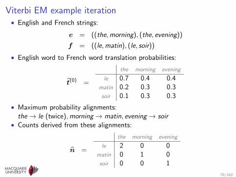
Viterbi EM example iteration• English and French strings:
e = ((the,morning), (the, evening))
f = ((le,matin), (le, soir))
• English word to French word translation probabilities:
t(0) =
the morning evening
le 0.7 0.4 0.4matin 0.2 0.3 0.3soir 0.1 0.3 0.3
• Maximum probability alignments:the→ le (twice),morning→ matin, evening→ soir
• Counts derived from these alignments:
n =
the morning evening
le 2 0 0matin 0 1 0soir 0 0 1
70/162
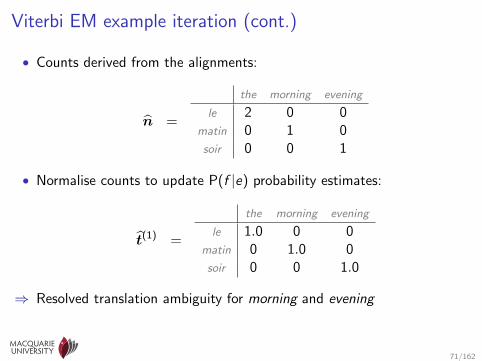
Viterbi EM example iteration (cont.)
• Counts derived from the alignments:
n =
the morning evening
le 2 0 0matin 0 1 0soir 0 0 1
• Normalise counts to update P(f |e) probability estimates:
t(1) =
the morning evening
le 1.0 0 0matin 0 1.0 0soir 0 0 1.0
⇒ Resolved translation ambiguity for morning and evening
71/162
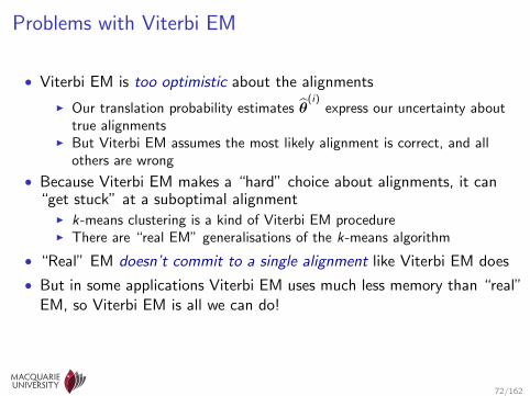
Problems with Viterbi EM
• Viterbi EM is too optimistic about the alignments
I Our translation probability estimates θ(i)
express our uncertainty abouttrue alignments
I But Viterbi EM assumes the most likely alignment is correct, and allothers are wrong
• Because Viterbi EM makes a “hard” choice about alignments, it can“get stuck” at a suboptimal alignment
I k-means clustering is a kind of Viterbi EM procedureI There are “real EM” generalisations of the k-means algorithm
• “Real” EM doesn’t commit to a single alignment like Viterbi EM does
• But in some applications Viterbi EM uses much less memory than “real”EM, so Viterbi EM is all we can do!
72/162

From Viterbi EM to EM
• The probability of aligning kth French word to jth English word:
P(Ak=j | E=e,Fk=f ) =θf ,ej∑m
j ′=1 θf ,ej′
• Viterbi EM assumes most probable alignment ak is true alignment
• EM distributes fractional counts according to P(Ak=j | E,Fk)
• Thought experiment: imagine e = (morning evening), f = (matin soir)occurs 1,000 times in our corpus
• Suppose our current model θ says P(matin→ evening) = 0.6 andP(matin→ morning) = 0.4
• Viterbi EM gives all 1,000 counts to (matin, evening)
• EM gives 600 counts to (matin, evening) and 400 counts to(matin,morning)
73/162

The EM algorithm for estimating translation probabilities
• The EM algorithm for estimating English word to French wordtranslation probabilities θ:
Initialise θ(0)
somehow (e.g., randomly)
For iterations i = 1, 2, . . . , :
E-step: compute the expected counts n(i) using θ(i−1)
M-step: set θ(i+1)
to the MLE for θ given n(i)
• Recall: the MLE (Maximum Likelihood Estimate) for θ is the relativefrequency
• The EM algorithm is guaranteed to converge to a local maximum
74/162

The E-step: calculating the expected counts
Clear n
For each sentence (f , e) in training data:
for each French word position k = 1, . . . , |f | :
for each English word position j = 1, . . . , |e| :
nfk ,ej + = P(Ak=j | E=e,Fk = fk)
Return n
• Recall that:
P(Ak=j | E=e,Fk=f ) =θf ,ej∑m
j ′=1 θf ,ej′
75/162

EM example iteration
• English word to French word translation probabilities:
t(0) =
the morning evening
le 0.7 0.4 0.4matin 0.2 0.3 0.3soir 0.1 0.3 0.3
• Probability of French to English alignments P(A | E,F )I Sentence 1: e = (the,morning),f = (le,matin)
P(A | E,F ) =le matin
the 0.64 0.4morning 0.36 0.6
I Sentence 2: e = (the, evening),f = (le, soir)
P(A | E,F ) =le soir
the 0.64 0.25evening 0.36 0.75
76/162

EM example iteration (cont.)• Probability of French to English alignments P(A | E,F )
I Sentence 1: e = (the,morning),f = (le,matin)
P(A | E,F ) =le matin
the 0.64 0.4morning 0.36 0.6
I Sentence 2: e = (the, evening),f = (le, soir)
P(A | E,F ) =le soir
the 0.64 0.25evening 0.36 0.75
• Expected counts derived from these alignments:
n =
the morning evening
le 1.28 0.36 0.36matin 0.4 0.6 0soir 0.25 0 0.75
77/162

EM example iteration (cont.)
• Expected counts derived from these alignments:
n =
the morning evening
le 1.28 0.36 0.36matin 0.4 0.6 0soir 0.25 0 0.75
• Normalise counts to estimate English word to French word probabilityestimates:
t(1) =
the morning evening
le 0.66 0.38 0.32matin 0.21 0.62 0soir 0.13 0 0.68
⇒ Resolved translation ambiguity for morning and evening
78/162

Determining convergence of the EM algorithm
• It’s possible to prove that an EM iteration never decreases the likelihoodof the data
I the likelihood is the probability of the training data under the currentmodel
I usually the likelihood increases rapidly with the first few iterations, andthen starts decreasing much slower
I often people just run 10 EM iterations
• Tracing the likelihood is a good way of debugging an EMimplementation
I the theorem says “likelihood never decreases”I but the likelihood can get extremely small⇒ to avoid underflow, calculate − log likelihood (which should decrease on
every iteration)
• It’s easy to calculate the likelihood while calculating the expectedcounts (see next slide)
79/162

Calculating the likelihood
• Recall: the probability of French word Fk = f is:
P(Fk=f | E=e) =1
|e|
|e|∑j=1
θf ,ej
• You need∑|e|
j=1 θfk ,ej to calculate the alignment probabilities anyway
P(Ak=j | E=e,Fk=fk) =θf ,ej∑m
j′=1 θf ,ej′
• The negative log likelihood is:
− log L =∑
(e,f)∈D
|f |∑k=1
− log P(Fk=fk | E=e)
=∑
(e,f)∈D
|f |∑k=1
− log1
|e|
|e|∑j=1
θfk ,ej
where the first sum is over all the sentence pairs in the training data
80/162

IBM1 − log likelihood on Hansards corpus
Iteration
− log L
107
5×10⁶
00 1 2 3 4 5 6 7 8 9 10
81/162

Alignments found by IBM1 from Hansards corpusthe le 0.36to a 0.29of de 0.58
and et 0.79in dans 0.24
that que 0.49a un 0.42is est 0.53i je 0.79it il 0.32
legislation loi 0.45federal federal 0.69
c c 0.69first premiere 0.37plan regime 0.58any ne 0.16only seulement 0.29must doit 0.26could pourrait 0.29how comment 0.43
add ajouter 0.32claims revendications 0.35achieve atteindre 0.21
else autre 0.37quality qualite 0.77
encourage encourager 0.28adopted adoptees 0.16success succes 0.60
representatives representants 0.70gave a 0.30
vinyl vinyle 0.29continuous maintient 0.06
tractor est 0.36briefs memoires 0.19
unethical ni 0.21rcms mrc 0.25
specifies montre 0.05proportionately proportionnellement 0.32
videos videos 0.23girlfriend amie 0.15
82/162
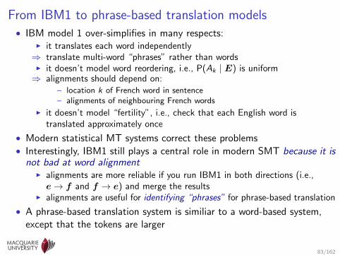
From IBM1 to phrase-based translation models• IBM model 1 over-simplifies in many respects:
I it translates each word independently⇒ translate multi-word “phrases” rather than wordsI it doesn’t model word reordering, i.e., P(Ak | E) is uniform⇒ alignments should depend on:
– location k of French word in sentence– alignments of neighbouring French words
I it doesn’t model “fertility”, i.e., check that each English word istranslated approximately once
• Modern statistical MT systems correct these problems• Interestingly, IBM1 still plays a central role in modern SMT because it is
not bad at word alignmentI alignments are more reliable if you run IBM1 in both directions (i.e.,e→ f and f → e) and merge the results
I alignments are useful for identifying “phrases” for phrase-based translation
• A phrase-based translation system is similiar to a word-based system,except that the tokens are larger
83/162

Identifying “phrases” given word alignments
They have full access to working documents
Ils
ont
acces
a
tous
le
documents
de
travail
84/162

Outline
Overview of computational linguistics and natural language processing
Key ideas in NLP and CL
Grammars and parsing
Conclusion and future directions
Non-parametric Bayesian extensions to grammars
85/162

Syntactic phrase structure and parsing
• Words compose to form phrases, whichrecursively compose to form larger phrasesand sentences
I this recursive structure can berepresented by a tree
I to “parse” a sentence means to identifyits structure
• Each phrase has a syntactic category
S
NP
D
the
N
cat
VP
V
chased
NP
D
the
N
dog
• Phrase structure helps identify semantic roles,i.e., who did what to whom
I Entities are typically noun phrasesI Propositions are often represented by sentences
• Syntactic parsing is currently used for:I named entity recognition and classificationI machine translationI automatic summarisation
86/162

Outline
Overview of computational linguistics and natural language processing
Key ideas in NLP and CL
Grammars and parsingContext-free grammarsProbabilistic context-free grammarsLearning probabilistic context-free grammarsParsing with PCFGs
Conclusion and future directions
Non-parametric Bayesian extensions to grammars
87/162

Context-Free Grammars
• Context-Free Grammars (CFGs) are a simple formal model ofcompositional syntax
• A probabilistic version of CFG is easy to formulate
• CFG parsing algorithms are comparatively simple
• We know that natural language is not context-free
⇒ more complex models, such as Chomsky’s transformational grammar
• But by splitting nonterminal labels PCFGs can approximate naturallanguage fairly well
• There are efficient dynamic-programming algorithms for ProbabilisticContext Free Grammar inference that can’t be expressed as graphicalmodel inference algorithms (as far as I know)
88/162

Informal presentation of CFGs
Grammar rules
S→ NP VPNP→ Det NVP→ V NPDet→ theDet→ aN→ catN→ dogV→ chasedV→ liked
Parse tree
S
89/162

Informal presentation of CFGs
Grammar rules
S→ NP VPNP→ Det NVP→ V NPDet→ theDet→ aN→ catN→ dogV→ chasedV→ liked
Parse tree
S
NP VP
89/162

Informal presentation of CFGs
Grammar rules
S→ NP VPNP→ Det NVP→ V NPDet→ theDet→ aN→ catN→ dogV→ chasedV→ liked
Parse tree
S
NP VP
Det N
89/162

Informal presentation of CFGs
Grammar rules
S→ NP VPNP→ Det NVP→ V NPDet→ theDet→ aN→ catN→ dogV→ chasedV→ liked
Parse tree
S
NP VP
Det N
the
89/162

Informal presentation of CFGs
Grammar rules
S→ NP VPNP→ Det NVP→ V NPDet→ theDet→ aN→ catN→ dogV→ chasedV→ liked
Parse tree
S
NP VP
Det N
the cat
89/162

Informal presentation of CFGs
Grammar rules
S→ NP VPNP→ Det NVP→ V NPDet→ theDet→ aN→ catN→ dogV→ chasedV→ liked
Parse tree
S
NP VP
Det N
the cat
V NP
89/162

Informal presentation of CFGs
Grammar rules
S→ NP VPNP→ Det NVP→ V NPDet→ theDet→ aN→ catN→ dogV→ chasedV→ liked
Parse tree
S
NP VP
Det N
the cat
V NP
chased
89/162

Informal presentation of CFGs
Grammar rules
S→ NP VPNP→ Det NVP→ V NPDet→ theDet→ aN→ catN→ dogV→ chasedV→ liked
Parse tree
S
NP VP
Det N
the cat
V NP
chased Det N
89/162

Informal presentation of CFGs
Grammar rules
S→ NP VPNP→ Det NVP→ V NPDet→ theDet→ aN→ catN→ dogV→ chasedV→ liked
Parse tree
S
NP VP
Det N
the cat
V NP
chased Det N
the
89/162

Informal presentation of CFGs
Grammar rules
S→ NP VPNP→ Det NVP→ V NPDet→ theDet→ aN→ catN→ dogV→ chasedV→ liked
Parse tree
S
NP VP
Det N
the cat
V NP
chased Det N
the dog
89/162

How to check if a CFG generates a tree• A CFG G = (N,V ,R, S) generates a labelled, finite, ordered tree t iff:
I t’s root node is labelled S ,I for every node n in t labelled with a terminal v ∈ V , n has no childrenI for every node n in t labelled with a nonterminal A ∈ N, there is a rule
A→ α ∈ R such that α is the sequence of labels of n’s children
[N = {S,NP,VP,Det,N,V} “N”s are different!
V = {the, a, cat, dog, chased, liked}
R =
S→ NP VP NP→ Det NVP→ V VP→ V NPDet→ a Det→ theN→ cat N→ dogV→ chased V→ liked
S
NP
Det
the
N
cat
VP
V
chased
NP
Det
the
N
dog
• A CFG G generates a string of terminals w iff w is the terminal yield ofa tree that G generates
I E.g., this CFG generates the cat chased the dog
90/162

CFGs can generate infinitely many trees
S→ NP VP VP→ V VP→ V SNP→ Sam NP→ Sasha V→ thinks V→ snores
S
NP
Sam
VP
V
snores
S
NP
Sasha
VP
V
thinks
S
NP
Sam
VP
V
snores
S
NP
Sam
VP
V
thinks
S
NP
Sasha
VP
V
thinks
S
NP
Sam
VP
V
snores
91/162

Syntactic ambiguity
• Ambiguity is pervasive in human languages
S
NP
I
VP
V
saw
NP
D
the
N
man
PP
P
with
NP
D
the
N
telescope
S
NP
I
VP
V
saw
NP
D
the
N
man
PP
P
with
NP
D
the
N
telescope
• Grammars can generate multiple trees with the same terminal yield
⇒ A combinatorial explosion in the number of parsesI number of parses usually is an exponential function of sentence lengthI some of our grammars generate more that 10100 parses for some sentences
92/162

What is “context free” about a CFG?• Grammars were originally viewed as string rewriting systems• A rule α→ β permits a string α to rewrite to string β
S→ NP VPNP→ dogsVP→ VV→ bark
S⇒ NP VP⇒ dogs VP⇒ dogs V⇒ dogs bark
• The Chomsky hierarchy of grammars is based on the shapes of α and βI Unrestricted: no restriction on α or β, undecidable recognitionI Context sensitive: |α| ≤ |β|, PSPACE-complete recognitionI Context free: |α| = 1, polynomial-time recognitionI Regular: |α| = 1, only one nonterminal at right edge in β,
linear time recognition (finite state machines)
• Context sensitive and unrestricted grammars don’t have muchapplication in NLP
• The mildly context-sensitive hierarchy lies between context-free andcontext-sensitive
93/162

Context-free grammars can over-generate• In a CFG, the possible expansions of a node depend only on its label
I how one node expands does not influence how other nodes expandI the label is the “state” of a CFG
• Example: the following grammar over-generates
S→ NP VP NP→ D N VP→ V NPNP→ she NP→ her D→ theV→ likes N→ cat
S
NP
she
VP
V
likes
NP
D
the
N
cat
S
NP
D
the
N
cat
VP
V
likes
NP
her
S
NP
her
VP
V
likes
NP
she
94/162

Outline
Overview of computational linguistics and natural language processing
Key ideas in NLP and CL
Grammars and parsingContext-free grammarsProbabilistic context-free grammarsLearning probabilistic context-free grammarsParsing with PCFGs
Conclusion and future directions
Non-parametric Bayesian extensions to grammars
95/162

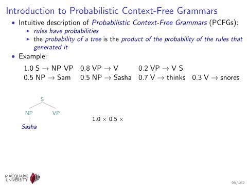
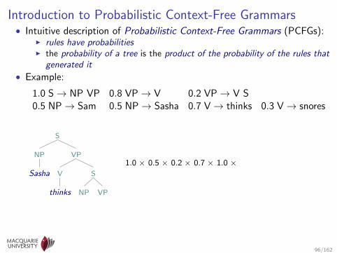
Introduction to Probabilistic Context-Free Grammars• Intuitive description of Probabilistic Context-Free Grammars (PCFGs):
I rules have probabilitiesI the probability of a tree is the product of the probability of the rules that
generated it
• Example:
1.0 S→ NP VP 0.8 VP→ V 0.2 VP→ V S0.5 NP→ Sam 0.5 NP→ Sasha 0.7 V→ thinks 0.3 V→ snores
S
96/162

Introduction to Probabilistic Context-Free Grammars• Intuitive description of Probabilistic Context-Free Grammars (PCFGs):
I rules have probabilitiesI the probability of a tree is the product of the probability of the rules that
generated it
• Example:
1.0 S→ NP VP 0.8 VP→ V 0.2 VP→ V S0.5 NP→ Sam 0.5 NP→ Sasha 0.7 V→ thinks 0.3 V→ snores
S
NP VP1.0 ×
96/162
Introduction to Probabilistic Context-Free Grammars• Intuitive description of Probabilistic Context-Free Grammars (PCFGs):
I rules have probabilitiesI the probability of a tree is the product of the probability of the rules that
generated it
• Example:
1.0 S→ NP VP 0.8 VP→ V 0.2 VP→ V S0.5 NP→ Sam 0.5 NP→ Sasha 0.7 V→ thinks 0.3 V→ snores
S
NP VP
Sasha1.0 × 0.5 ×
96/162

Introduction to Probabilistic Context-Free Grammars• Intuitive description of Probabilistic Context-Free Grammars (PCFGs):
I rules have probabilitiesI the probability of a tree is the product of the probability of the rules that
generated it
• Example:
1.0 S→ NP VP 0.8 VP→ V 0.2 VP→ V S0.5 NP→ Sam 0.5 NP→ Sasha 0.7 V→ thinks 0.3 V→ snores
S
NP VP
Sasha V S
1.0 × 0.5 × 0.2 ×
96/162

Introduction to Probabilistic Context-Free Grammars• Intuitive description of Probabilistic Context-Free Grammars (PCFGs):
I rules have probabilitiesI the probability of a tree is the product of the probability of the rules that
generated it
• Example:
1.0 S→ NP VP 0.8 VP→ V 0.2 VP→ V S0.5 NP→ Sam 0.5 NP→ Sasha 0.7 V→ thinks 0.3 V→ snores
S
NP VP
Sasha V S
thinks
1.0 × 0.5 × 0.2 × 0.7 ×
96/162
Introduction to Probabilistic Context-Free Grammars• Intuitive description of Probabilistic Context-Free Grammars (PCFGs):
I rules have probabilitiesI the probability of a tree is the product of the probability of the rules that
generated it
• Example:
1.0 S→ NP VP 0.8 VP→ V 0.2 VP→ V S0.5 NP→ Sam 0.5 NP→ Sasha 0.7 V→ thinks 0.3 V→ snores
S
NP VP
Sasha V S
thinks NP VP
1.0 × 0.5 × 0.2 × 0.7 × 1.0 ×
96/162

Introduction to Probabilistic Context-Free Grammars• Intuitive description of Probabilistic Context-Free Grammars (PCFGs):
I rules have probabilitiesI the probability of a tree is the product of the probability of the rules that
generated it
• Example:
1.0 S→ NP VP 0.8 VP→ V 0.2 VP→ V S0.5 NP→ Sam 0.5 NP→ Sasha 0.7 V→ thinks 0.3 V→ snores
S
NP VP
Sasha V S
thinks NP VP
Sam
1.0 × 0.5 × 0.2 × 0.7 × 1.0 × 0.5 ×
96/162

Introduction to Probabilistic Context-Free Grammars• Intuitive description of Probabilistic Context-Free Grammars (PCFGs):
I rules have probabilitiesI the probability of a tree is the product of the probability of the rules that
generated it
• Example:
1.0 S→ NP VP 0.8 VP→ V 0.2 VP→ V S0.5 NP→ Sam 0.5 NP→ Sasha 0.7 V→ thinks 0.3 V→ snores
S
NP VP
Sasha V S
thinks NP VP
Sam V
1.0 × 0.5 × 0.2 × 0.7 × 1.0 × 0.5 × 0.8 ×
96/162

Introduction to Probabilistic Context-Free Grammars• Intuitive description of Probabilistic Context-Free Grammars (PCFGs):
I rules have probabilitiesI the probability of a tree is the product of the probability of the rules that
generated it
• Example:
1.0 S→ NP VP 0.8 VP→ V 0.2 VP→ V S0.5 NP→ Sam 0.5 NP→ Sasha 0.7 V→ thinks 0.3 V→ snores
S
NP VP
Sasha V S
thinks NP VP
Sam V
snores
1.0 × 0.5 × 0.2 × 0.7 × 1.0 × 0.5 × 0.8 × 0.3 = 0.0084
96/162

Probabilistic Context-Free Grammars (PCFGs)
• A PCFG is a 5-tuple (N,V ,R,S , p) where:I (N,V ,R,S) is a CFGI p maps each rule in R to a value in [0, 1] where for each nonterminal
A ∈ N: ∑A→α∈RA
pA→α = 1.0
where RA is the subset of rules in R expanding A
• Example:1.0 S→ NP VP0.8 VP→ V 0.2 VP→ V S0.5 NP→ Sam 0.5 NP→ Sasha0.7 V→ thinks 0.3 V→ snores
97/162

PCFGs define probability distributions over trees
• A CFG G defines a (possibly infinite) set of trees TG• A PCFG G defines a probability PG (t) for each t ∈ TG
I P(t) is the product of the pA→α of the rules A→ α used to generate tI If nA→α(t) is the number of times rule A→ α is used in generating t,
then
P(t) =∏
A→α∈R
pnA→α(t)A→α
• Example: If t is the following tree:S
NP
Sam
VP
V
snores
then nNP→Sam(t) = 1 and nV→thinks(t) = 0
98/162

PCFGs define probability distributions over strings ofterminals• The yield of a tree is the sequence of its leaf labels
I Example:
yield
S
NP
Sam
VP
V
snores
= Sam snores
• If x is a string of terminals, let TG (x) be the subset of trees in TG withyield x
• Then the probability of a terminal string x is the sum of theprobabilities of trees with yield x , i.e.:
PG (x) =∑
t∈TG (x)
PG (t)
⇒ PCFGs can be used as language models99/162

PCFGs as recursive mixture distributions
• Given the PCFG rule:A→ B1 . . . Bn
the distribution over strings for A is the concatenation of the product ofthe distributions for B1, . . . ,Bn
• Given the two PCFGs rules:
A→ B A→ C
the distribution over strings for A are a mixture of the distributions overstrings for B and C with weights pA→B and pA→C
• A PCFG with the rules:
A→ AB A→ C
defines a recursive mixture distribution where the strings of A beginwith a C followed by zero or more Bs, with probabilities decaying as anexponential function of the number of Bs.
100/162

Outline
Overview of computational linguistics and natural language processing
Key ideas in NLP and CL
Grammars and parsingContext-free grammarsProbabilistic context-free grammarsLearning probabilistic context-free grammarsParsing with PCFGs
Conclusion and future directions
Non-parametric Bayesian extensions to grammars
101/162

Treebank corpora contain phrase-structure analyses
• A treebank is a corpus where every sentence has been (manually) parsedI the Penn WSJ treebank has parses for 49,000 sentences
S
NP-SBJ
DT
The
JJ
new
NNS
options
VP
VBP
carry
PRT
RP
out
NP
NP
NN
part
PP
IN
of
NP
NP
DT
an
NN
agreement
SBAR
WHNP-12
IN
that
S
NP-SBJ-1
DT
the
NN
pension
NN
fund
,
,
S-ADV
NP-SBJ
-NONE-
*-1
PP-PRD
IN
under
NP
NN
pressure
S
NP-SBJ
-NONE-
*
VP
VP
TO
to
VP
VB
relax
NP
PRP$
its
JJ
strict
NN
participation
NNS
rules
CC
and
VP
TO
to
VP
VB
provide
NP
JJR
more
NN
investment
NNS
options
,
,
VP
VBN
reached
NP
-NONE-
*T*-12
PP
IN
with
NP
DT
the
NNP
SEC
PP-TMP
IN
in
NP
NNP
December
.
.
102/162

Learning PCFGs from treebanks
• Learning a PCFG from a treebank DI Count how often each rule A→ α and each nonterminal A appears in DI Relative frequency a.k.a. Maximum Likelihood estimator:
pA→α =nA→αnA
, where:
nA→α = number of times A→ α is used in D
nA = number of times A appears in D
I Add-1 smoothed estimator:
pA→α =nA→α + 1
nA + |RA|, where:
RA = subset of rules R that expand nonterminal A
103/162

Learning PCFGs from treebanks example (1)
D =
S
NP
she
VP
V
likes
NP
D
the
N
cat
S
NP
D
the
N
cat
VP
V
likes
NP
her
S
NP
Sam
VP
V
purrs
• Nonterminal counts:
nS = 3 nNP = 5 nVP = 3nD = 2 nN = 2 nV = 3
• Rule counts:
nS→NP VP = 3 nVP→V NP = 2 nVP→V = 1nNP→D N = 2 nNP→she = 1 nNP→her = 1nNP→Sam = 1 nD→the = 2 nN→cat = 2nV→likes = 2 nV→purrs = 1
104/162

Learning PCFGs from treebanks example (2)
• Nonterminal counts:
nS = 3 nNP = 5 nVP = 3nD = 2 nN = 2 nV = 3
• Rule counts:
nS→NP VP = 3 nVP→V NP = 2 nVP→V = 1nNP→D N = 2 nNP→she = 1 nNP→her = 1nNP→Sam = 1 nD→the = 2 nN→cat = 2nV→likes = 2 nV→purrs = 1
• Estimated rule probabilities:
pS→NP VP = 3/3 pVP→V NP = 2/3 pVP→V = 1/3pNP→D N = 2/5 pNP→she = 1/5 pNP→her = 1/5pNP→Sam = 1/5 pD→the = 2/2 pN→cat = 2/2pV→likes = 2/3 pV→purrs = 1/3
105/162

Accuracy of treebank PCFGs
• Parser accuracy is usually measured by f-score on a held-out test corpus
• A treebank PCFG (as described above) does fairly poorly (≈ 0.7 f-score)
• Accuracy can be improved by refining the categoriesI wide variety of programmed and fully automatic category-splitting
proceduresI modern PCFG parsers achieve f-score ≈ 0.9
• Category splitting dramatically increases the number of categories, andhence rules and parameters in PCFG
I recall bias-variance tradeoff: category splitting reduces bias, but increasesvariance
⇒ smoothing is essential, and details of smoothing procedure make a bigimpact on parser f-score
106/162

Parent annotation of a treebank
• Parent annotation is a simple category-splitting procedure where theparent’s label is added to every non-terminal label
• Original trees:S
NP
she
VP
V
likes
NP
D
the
N
cat
S
NP
D
the
N
cat
VP
V
likes
NP
her
• After parent annotation:S
NPˆS
she
VPˆS
VˆVP
likes
NPˆVP
DˆNP
the
NˆNP
cat
S
NPˆS
DˆNP
the
NˆNP
cat
VPˆS
VˆVP
likes
NPˆVP
her
107/162

Why does parent annotation improve parser accuracy?
• After parent annotation:
S
NPˆS
she
VPˆS
VˆVP
likes
NPˆVP
DˆNP
the
NˆNP
cat
S
NPˆS
DˆNP
the
NˆNP
cat
VPˆS
VˆVP
likes
NPˆVP
her
• Parent annotation adds important linguistic contextI rules NP→ she and NP→ her get replaced with
NPˆS→ she and NPˆVP→ her⇒ no longer over-generates her likes she
• But number of rules grows: the Penn WSJ treebank inducesI 74,169 rules before parent annotationI 93,386 rules after parent annotation
• So sparse data becomes more of a problem after parent annotation
108/162

Outline
Overview of computational linguistics and natural language processing
Key ideas in NLP and CL
Grammars and parsingContext-free grammarsProbabilistic context-free grammarsLearning probabilistic context-free grammarsParsing with PCFGs
Conclusion and future directions
Non-parametric Bayesian extensions to grammars
109/162

Goal of PCFG parsing
• Given a PCFG G and a string of terminals x , we want to find the mostprobable parse tree t(x) in the set of parses TG (x) that G generates forx
t(x) = argmaxt∈TG (x)
PG (t)
• Naive algorithm to find t(x):I enumerate all trees with a terminal yield of length |x |I if yield(t) = x and PG (t) is greater than probability of best tree seen so
far, keep t and PG (t)I return tree with highest probability
110/162

Why is PCFG parsing hard?
• Broad-brush ideas behind probabilistic parsing:I to avoid problems of coverage and robustness, grammar generates all
possible parses (or at least most of the possibly useful ones)I probability distribution distinguishes “good” parses from “bad” ones
⇒ Even moderately long sentences have an astronomical number of parsesI there are sentences in WSJ PTB with over 10100 parses
⇒ no hope that parsing via exhaustive enumeration will be practical
111/162

High-level overview of PCFG parsing
• All the efficient PCFG parsers I know of involve two steps:I binarise grammar, i.e., transform it so it has no rules A→ α where|α| > 2
– this can be done as a pre-processing step, or– on-the-fly as part of the parsing algorithm
I use dynamic programming to search for optimal parses of substrings of x
• Together these permit us to parse e.g., 100-word sentences in millions orbillions of operations (rather than the 10100 that the naive algorithmrequires)
112/162
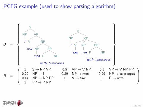
PCFG example (used to show parsing algorithm)
D =
S
NP
I
VP
V
saw
NP
NP
men
PP
P
with
NP
telescopes
S
NP
I
VP
V
saw
NP
men
PP
P
with
NP
telescopes
R =
1 S→ NP VP 0.5 VP→ V NP 0.5 VP→ V NP PP
0.29 NP→ I 0.29 NP→ men 0.29 NP→ telescopes0.14 NP→ NP PP 1 V→ saw 1 P→ with
1 PP→ P NP
113/162

Rule binarisation• Our dynamic programming algorithm requires all rules to have at most
two children• Binarisation: replace ternary and longer rules with a sequence of binary
rulesI replace rule p A → B1 B2 . . . Bm with rules
p A→ B1 B2 . . . Bm−1 Bm
1.0 B1 B2 . . . Bm−1 → B1 B2 . . . Bm−2 Bm−1
1.0 B1 B2 → B1 B2
• Example: rule 0.5 VP→ V NP PP is replaced with:
0.5 VP → V NP PP1.0 V NP → V NP
• This can expand the number of rules in the grammarI The WSJ PTB PCFG has:
– 74,619 rules before binarisation– 89,304 rules after binarisation– 109,943 rules with both binarisation and parent annotation
114/162

PCFG example after binarisation
D =
S
NP
I
VP
V
saw
NP
NP
men
PP
P
with
NP
telescopes
S
NP
I
VP
V NP
V
saw
NP
men
PP
P
with
NP
telescopes
R =
1 S→ NP VP 0.5 VP→ V NP 0.29 NP→ I0.29 NP→ men 0.29 NP→ telescopes 0.14 NP→ NP PP
1 V→ saw 1 PP→ P NP 1 P→ with0.5 VP → V NP PP 1 V NP → V NP
115/162
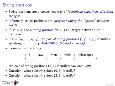
String positions
• String positions are a convenient way of identifying substrings of a fixedstring x
• Informally, string positions are integers naming the “spaces” betweenwords
• If |x | = n, the a string position for x is an integer between 0 to ninclusive
• If x = (x0, . . . , xn−1), the pair of string positions (i , j), i ≤ j identifiessubstring xi , . . . , xj−1. WARNING: 0-based indexing!
• Example: In the string
| I | saw | men | with | telescopes |0 1 2 3 4 5
the pair of string positions (1, 4) identifies saw men with
• Question: what substring does (0, 5) identify?
• Question: what substring does (2, 2) identify?
116/162

Chomsky-normal form
• We’ll assume that our PCFG G is in Chomsky-normal form (CNF), i.e.,every rule is of the form:
I A→ B C , where A,B,C ∈ N (i.e., A,B,C are nonterminals), orI A→ v , where v ∈ V (i.e., A is a nonterminal and v is a terminal)
• Binarisation is a key step in bringing arbitrary PCFGs into CNF• Our example grammar is in CNF
1 S→ NP VP 0.5 VP→ V NP 0.29 NP→ I0.29 NP→ men 0.29 NP→ telescopes 0.14 NP→ NP PP
1 V→ saw 1 PP→ P NP 1 P→ with0.5 VP → V NP PP 1 V NP → V NP
117/162

Introduction to dynamic programming parsing
• Key idea: find most probable parse trees with top node A for eachsubstring (i , k) of string x
I find most probable parse trees for shorter substrings firstI use these to find most probable parse trees for longer substrings
• If k = i + 1, then most probable parse tree is A→ xi• If k > i + 1 then most probable parse tree for A can only be formed by:
I finding a mid-point j , where i < j < k , andI combining a most probable parse tree for B spanning (i , j) withI a most probable parse tree for C spanning (j , k)I using some rule A→ B C ∈ R
0 i j k n
B C
A
118/162

Dynamic programming parsing algorithm
• Given a PCFG G = (N,V ,R, S , p) in CNF and a string x where |x | = n,fill a table Q[A, i , k] for each A ∈ N and 0 ≤ i < k ≤ n
I Q[A, i , k] will be set to the maximum probability of any parse with topnode A spanning (i , k)
• Algorithm:for each i = 0, . . . , n − 1:Q[A, i , i + 1] = pA→xi
for ` = 2, . . . , n :for i = 0, . . . , n − ` :k = i + `for each A ∈ N :Q[A, i , k] = max
jmax
A→B CpA→B C Q[B, i , j ] Q[C , j , k]
return Q[S , 0, n] (max probability of S)
• In recursion, the midpoint j ranges over i + 1, . . . , k − 1,and the rule A→ B C ranges over all rules with parent A
• Keep back-pointers from each Q[A, i , k] to optimal children
119/162

Dynamic programming parsing example
• Grammar in CNF:
1 S→ NP VP 0.5 VP→ V NP 0.29 NP→ I0.29 NP→ men 0.29 NP→ telescopes 0.14 NP→ NP PP
1 V→ saw 1 PP→ P NP 1 P→ with0.5 VP → V NP PP 1 V NP → V NP
• String x to parse:
| I | saw | men | with | telescopes |
0 1 2 3 4 5
• Base case (` = 1)
Q[NP, 0, 1] = 0.29 Q[V, 1, 2] = 1 Q[NP, 2, 3] = 0.29Q[P, 3, 4] = 1 Q[NP, 4, 5] = 0.29
• Recursive case ` = 2:
Q[VP, 1, 3] = 0.15 from Q[V, 1, 2] and Q[NP, 2, 3]Q[V NP, 1, 3] = 0.29 from Q[V, 1, 2] and Q[NP, 2, 3]
Q[PP, 3, 5] = 0.29 from Q[P, 3, 4] and Q[NP, 4, 5]
120/162

Dynamic programming parsing example (cont)
• Recursive case ` = 3:
Q[S, 0, 3] = 0.044 from Q[NP, 0, 1] and Q[VP, 1, 3]Q[NP, 2, 5] = 0.011 from Q[NP, 2, 3] and Q[PP, 3, 5]
• Recursive case ` = 4:
Q[VP, 1, 5] = 0.042 from Q[V NP, 1, 3] and Q[PP, 3, 5]
(alternative parse from Q[V, 1, 2] and Q[NP, 2, 5] only has probability 0.0055)
• Recursive case ` = 6:
Q[S, 0, 5] = 0.012 from Q[NP, 0, 1] and Q[VP, 1, 5]
• By chasing backpointers, we find the following parse:
(S (NP I) (VP (V NP (V saw) (NP men)) (PP (P with) (NP telescopes))))
• After removing the “binarisation categories”:
(S (NP I) (VP (V saw) (NP men) (PP (P with) (NP telescopes))))
121/162

Running time of dynamic programming parsing
• The dynamic programming parsing algorithm enumerates all possiblestring positions 0 ≤ i < j < k ≤ n, where n = |x | is the length of thestring to be parsed
• There are O(n3) of these, so this will take O(n3) time
• For each possible (i , j , k) triple, it considers all m = |R| rules in thegrammar. This takes O(m) time.
⇒ The dynamic programming parsing algorithm runs in O(mn3) time
• This is much better than the exponential time of the naive algorithm,but with large grammars it can still be very slow
• Question: what are the space requirements of the algorithm?
122/162

State of the art parsing algorithms
• State-of-the-art syntactic parsers come in two varieties: phrase structureand dependency parsers
• Phrase structure parsers are often effectively PCFGs with hundreds ofthousands of states
I “coarse to fine” search algorithms using dynamic programmingI discriminatively trained, with the PCFG probability as a “feature”
• Dependency parsers are often incremental shift-reduce parsers withoutdynamic programming
I each move is predicted locally by a classifierI beam search to avoid “garden pathing”
• State-of-the-art systems achieve over 90% f-score (accuracy)
• Major internet companies are reported to parse the web several times aday
123/162

Outline
Overview of computational linguistics and natural language processing
Key ideas in NLP and CL
Grammars and parsing
Conclusion and future directions
Non-parametric Bayesian extensions to grammars
124/162

Summary
• Computational linguistics and natural language processing:I were originally inspired by linguistics,I but now they are almost applications of machine learning and statistics
• But they are unusual ML applications because they involve predictingvery highly structured objects
I phrase structure trees in syntactic parsingI entire sentences in speech recognition and machine translation
• We solve these problems using standard methods from machine learning:
I define a probabilistic model over the relevant variablesI factor the model into small components that we can learnI examples: HMMs, CRFs and PCFGs
• Often the relevant variables are not available in the training dataI Expectation-Maximisation, MCMC, etc. can impute the values of the
hidden variables
125/162
The future of NLP
• NLP applications are exploding, driven mainly by:I the information explosion (much of which is text)I the mobile computing revolution (talk with our computers)
• The major internet companies are investing in NLP at a scale not seenbefore
I the knowledge graph and similiar information repositories provide muchricher information than available before
• Topic modelling and opinion mining likely to be widely used to trackrapidly changing document collections (e.g., social media)
126/162
Good areas for future research
• Improving existing NLP and CL models (parsing, relation extraction,machine translation, etc.)
I explore new modelsI apply new ideas from machine learning, e.g., deep learning
• Combine and extend models to produce new NLP applicationsI parse speech data (and detect/correct speech disfluencies)
• Find new knowledge sources (e.g., kinds of training data) or new waysof exploiting existing ones
I use the Knowledge Graph and similiar resources to improve parsing andinformation extraction
• Develop models in which natural language is just one of the kinds ofinformation used
I integrate language and visionI integrate language with external database (e.g., financial data, health
records)
127/162

Deeper questions facing the field
• Our scientific understanding of semantics (meanings), world knowledgeand real-world inference is still very poor
I can existing methods scale up, or will we need a radical breakthrough?
• NLP (like most of ML) reduces learning to optimisationI we have good methods for estimating weights for featuresI but identifying possibly-useful features is a “black art”
• Hierarchical non-parametric Bayesian methods offer a mathematicalframework for learning the relevant features as well as their weights
I the base distribution generates (a possibly infinite number of) potentiallyuseful elements
I from which a finite subset are actually instantiated, based on the dataI the algorithms simultaneously search for useful elements and learn their
weights
128/162

Outline
Overview of computational linguistics and natural language processing
Key ideas in NLP and CL
Grammars and parsing
Conclusion and future directions
Non-parametric Bayesian extensions to grammars
129/162
PCFGs as products of multinomials
• The choice of rule to expand a state in an HMM or a nonterminal in aPCFG is a draw from a multinomial distribution
⇒ HMMs and PCFGs can be viewed as products of multinomialdistributions
⇒ Dirichlet distributions are conjugate priors for HMMs and PCFGsI Bayesian inference for HMMs and PCFGs generally assumes Dirichlet
priors
⇒ Non-parametric generalisations of multinomials should also let usgeneralise HMMs and PCFGs
130/162

Outline
Overview of computational linguistics and natural language processing
Key ideas in NLP and CL
Grammars and parsing
Conclusion and future directions
Non-parametric Bayesian extensions to grammarsA non-parametric extension to Dirichlet-MultinomialsAdaptor grammars
131/162

Bayesian inference for Dirichlet-multinomials
• Predictive probability (probability of next event) with uniform Dirichletprior with mass α over m outcomes and observed dataZ1:n = (Z1, . . . ,Zn)
P(Zn+1 = k | Z1:n, α) ∝ nk(Z1:n) + α/m
where nk(Z1:n) is number of times k appears in Z1:n
• Example: Coin (m = 2), α = 1, Z1:2 = (heads, heads)I P(Z3 = heads | Z1:2, α) ∝ 2.5I P(Z3 = tails | Z1:2, α) ∝ 0.5
132/162

Dirichlet-multinomials with many outcomes
• Predictive probability:
P(Zn+1 = k | Z1:n, α) ∝ nk(Z1:n) + α/m
• Suppose the number of outcomes m� n. Then:
P(Zn+1 = k | Z1:n, α) ∝
nk(Z1:n) if nk(Z1:n) > 0
α/m if nk(Z1:n) = 0
• But most outcomes will be unobserved, so:
P(Zn+1 6∈ Z1:n | Z1:n, α) ∝ α
133/162

From Dirichlet-multinomials to Chinese RestaurantProcesses
. . .
• Suppose number of outcomes is unboundedbut we pick the event labels
• If we number event types in order of occurrence⇒ Chinese Restaurant Process
Z1 = 1
P(Zn+1 = k | Z1:n, α) ∝{
nk(Z1:n) if k ≤ m = max(Z1:n)α if k = m + 1
134/162

Chinese Restaurant Process (0)
• Customer→ table mapping Z =
• P(z) = 1
• Next customer chooses a table according to:
P(Zn+1 = k | Z1:n) ∝{
nk(Z1:n) if k ≤ m = max(Z1:n)α if k = m + 1
135/162

Chinese Restaurant Process (1)
α
• Customer→ table mapping Z = 1
• P(z) = α/α
• Next customer chooses a table according to:
P(Zn+1 = k | Z1:n) ∝{
nk(Z1:n) if k ≤ m = max(Z1:n)α if k = m + 1
136/162

Chinese Restaurant Process (2)
1 α
• Customer→ table mapping Z = 1, 1
• P(z) = α/α× 1/(1 + α)
• Next customer chooses a table according to:
P(Zn+1 = k | Z1:n) ∝{
nk(Z1:n) if k ≤ m = max(Z1:n)α if k = m + 1
137/162

Chinese Restaurant Process (3)
2 α
• Customer→ table mapping Z = 1, 1, 2
• P(z) = α/α× 1/(1 + α)× α/(2 + α)
• Next customer chooses a table according to:
P(Zn+1 = k | Z1:n) ∝{
nk(Z1:n) if k ≤ m = max(Z1:n)α if k = m + 1
138/162

Chinese Restaurant Process (4)
2 1 α
• Customer→ table mapping Z = 1, 1, 2, 1
• P(z) = α/α× 1/(1 + α)× α/(2 + α)× 2/(3 + α)
• Next customer chooses a table according to:
P(Zn+1 = k | Z1:n) ∝{
nk(Z1:n) if k ≤ m = max(Z1:n)α if k = m + 1
139/162

Labeled Chinese Restaurant Process (0)
• Table→ label mapping Y =
• Customer→ table mapping Z =
• Output sequence X =
• P(X) = 1
• Base distribution P0(Y ) generates a label Yk for each table k
• All customers sitting at table k (i.e., Zi = k) share label Yk
• Customer i sitting at table Zi has label Xi = YZi
140/162
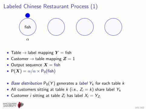
Labeled Chinese Restaurant Process (1)
fish
α
• Table→ label mapping Y = fish
• Customer→ table mapping Z = 1
• Output sequence X = fish
• P(X) = α/α× P0(fish)
• Base distribution P0(Y ) generates a label Yk for each table k
• All customers sitting at table k (i.e., Zi = k) share label Yk
• Customer i sitting at table Zi has label Xi = YZi
141/162

Labeled Chinese Restaurant Process (2)
fish
1 α
• Table→ label mapping Y = fish
• Customer→ table mapping Z = 1, 1
• Output sequence X = fish,fish
• P(X) = P0(fish)× 1/(1 + α)
• Base distribution P0(Y ) generates a label Yk for each table k
• All customers sitting at table k (i.e., Zi = k) share label Yk
• Customer i sitting at table Zi has label Xi = YZi
142/162

Labeled Chinese Restaurant Process (3)
fish
2
apple
α
• Table→ label mapping Y = fish,apple
• Customer→ table mapping Z = 1, 1, 2
• Output sequence X = fish,fish,apple
• P(X) = P0(fish)× 1/(1 + α)× α/(2 + α)P0(apple)
• Base distribution P0(Y ) generates a label Yk for each table k
• All customers sitting at table k (i.e., Zi = k) share label Yk
• Customer i sitting at table Zi has label Xi = YZi
143/162
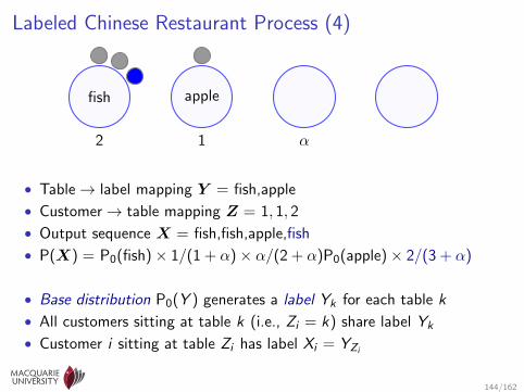
Labeled Chinese Restaurant Process (4)
fish
2
apple
1 α
• Table→ label mapping Y = fish,apple
• Customer→ table mapping Z = 1, 1, 2
• Output sequence X = fish,fish,apple,fish
• P(X) = P0(fish)× 1/(1 + α)× α/(2 + α)P0(apple)× 2/(3 + α)
• Base distribution P0(Y ) generates a label Yk for each table k
• All customers sitting at table k (i.e., Zi = k) share label Yk
• Customer i sitting at table Zi has label Xi = YZi
144/162

Summary: Chinese Restaurant Processes
• Chinese Restaurant Processes (CRPs) generalize Dirichlet-Multinomialsto an unbounded number of outcomes
I concentration parameter α controls how likely a new outcome isI CRPs exhibit a rich get richer power-law behaviour
• Labeled CRPs use a base distribution to label each tableI base distribution can have infinite supportI concentrates mass on a countable subsetI power-law behaviour ⇒ Zipfian distributions
145/162

Nonparametric extensions of PCFGs
• Chinese restaurant processes are a nonparametric extension ofDirichlet-multinomials because the number of states (occupied tables)depends on the data
• Two obvious nonparametric extensions of PCFGs:I let the number of nonterminals grow unboundedly
– refine the nonterminals of an original grammare.g., S35 → NP27 VP17
⇒ infinite PCFG
I let the number of rules grow unboundedly
– “new” rules are compositions of several rules from original grammar– equivalent to caching tree fragments⇒ adaptor grammars
• No reason both can’t be done together . . .
146/162

Outline
Overview of computational linguistics and natural language processing
Key ideas in NLP and CL
Grammars and parsing
Conclusion and future directions
Non-parametric Bayesian extensions to grammarsA non-parametric extension to Dirichlet-MultinomialsAdaptor grammars
147/162

Adaptor grammars: informal description
• The trees generated by an adaptor grammar are defined by CFG rules asin a CFG
• A subset of the nonterminals are adapted
• Unadapted nonterminals expand by picking a rule and recursivelyexpanding its children, as in a PCFG
• Adapted nonterminals can expand in two ways:I by picking a rule and recursively expanding its children, orI by generating a previously generated tree (with probability proportional to
the number of times previously generated)
• Implemented by having a CRP for each adapted nonterminal
• The CFG rules of the adapted nonterminals determine the basedistributions of these CRPs
148/162
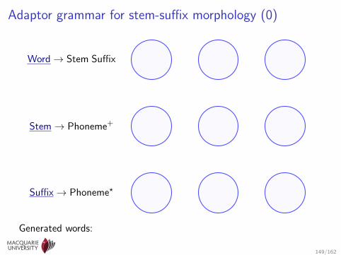
Adaptor grammar for stem-suffix morphology (0)
Word→ Stem Suffix
Stem→ Phoneme+
Suffix→ Phoneme?
Generated words:
149/162

Adaptor grammar for stem-suffix morphology (1a)
Word→ Stem Suffix
Stem→ Phoneme+
Suffix→ Phoneme?
Generated words:
150/162

Adaptor grammar for stem-suffix morphology (1b)
Word→ Stem Suffix
Stem→ Phoneme+
Suffix→ Phoneme?
Generated words:
151/162
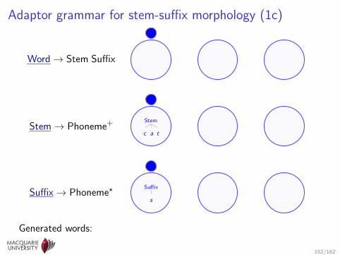
Adaptor grammar for stem-suffix morphology (1c)
Word→ Stem Suffix
Stem→ Phoneme+ Stem
c a t
Suffix→ Phoneme?Suffix
s
Generated words:
152/162

Adaptor grammar for stem-suffix morphology (1d)
Word→ Stem SuffixWord
Stem
c a t
Suffix
s
Stem→ Phoneme+ Stem
c a t
Suffix→ Phoneme?Suffix
s
Generated words: cats
153/162

Adaptor grammar for stem-suffix morphology (2a)
Word→ Stem SuffixWord
Stem
c a t
Suffix
s
Stem→ Phoneme+ Stem
c a t
Suffix→ Phoneme?Suffix
s
Generated words: cats
154/162

Adaptor grammar for stem-suffix morphology (2b)
Word→ Stem SuffixWord
Stem
c a t
Suffix
s
Stem→ Phoneme+ Stem
c a t
Suffix→ Phoneme?Suffix
s
Generated words: cats
155/162
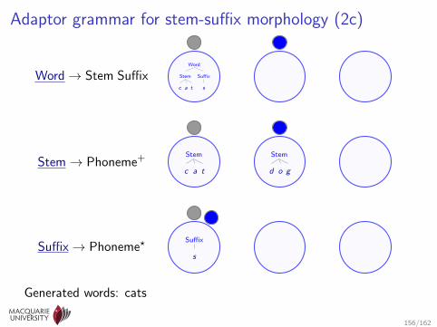
Adaptor grammar for stem-suffix morphology (2c)
Word→ Stem SuffixWord
Stem
c a t
Suffix
s
Stem→ Phoneme+ Stem
c a t
Stem
d o g
Suffix→ Phoneme?Suffix
s
Generated words: cats
156/162
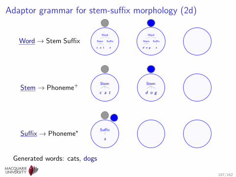
Adaptor grammar for stem-suffix morphology (2d)
Word→ Stem SuffixWord
Stem
c a t
Suffix
s
Word
Stem
d o g
Suffix
s
Stem→ Phoneme+ Stem
c a t
Stem
d o g
Suffix→ Phoneme?Suffix
s
Generated words: cats, dogs
157/162

Adaptor grammar for stem-suffix morphology (3)
Word→ Stem SuffixWord
Stem
c a t
Suffix
s
Word
Stem
d o g
Suffix
s
Stem→ Phoneme+ Stem
c a t
Stem
d o g
Suffix→ Phoneme?Suffix
s
Generated words: cats, dogs, cats
158/162

Adaptor grammars as generative processes
• The sequence of trees generated by an adaptor grammar are notindependent
I it learns from the trees it generatesI if an adapted subtree has been used frequently in the past, it’s more likely
to be used again
• but the sequence of trees is exchangable (important for sampling)
• An unadapted nonterminal A expands using A→ β with probabilityθA→β
• Each adapted nonterminal A is associated with a CRP (or PYP) thatcaches previously generated subtrees rooted in A
• An adapted nonterminal A expands:I to a subtree τ rooted in A with probability proportional to the number of
times τ was previously generatedI using A → β with probability proportional to αAθA→β
159/162

Properties of adaptor grammars
• Possible trees are generated by CFG rulesbut the probability of each adapted tree is learned separately
• Probability of adapted subtree τ is proportional to:I the number of times τ was seen before⇒ “rich get richer” dynamics (Zipf distributions)
I plus αA times prob. of generating it via PCFG expansion
⇒ Useful compound structures can be more probable than their parts
• PCFG rule probabilities estimated from table labels⇒ effectively learns from types, not tokens⇒ makes learner less sensitive to frequency variation in input
160/162

Applications of adaptor grammars
• Main application until now has been in modelling human languageacquisition
I unsupervised word segmentationI exploring the role of
– information about the non-linguistic context– syllabic structure– prosodic structure
• By exploiting the connection between PCFGs and LDA topic models, wecan:
I develop topical collocation modelse.g., New York Times, White House
I learn the structure of proper namese.g., Mr Pierre E. van Winken
161/162

Interested in Machine Learning and Computational Linguistics?
We’re recruiting bright PhD students.
Contact [email protected] for more information.
162/162