introduction to complexity and computability -...

Introduction to Complexity and ComputabilityNTIN090

Jirka Finkhttps://ktiml.mff.cuni.cz/˜fink/

Department of Theoretical Computer Science and Mathematical LogicFaculty of Mathematics and Physics

Charles University in Prague

Winter semester 2017/18Last change on January 11, 2018

License: Creative Commons BY-NC-SA 4.0

Jirka Fink Introduction to Complexity and Computability 1

https://ktiml.mff.cuni.cz/~fink/

https://creativecommons.org/licenses/by-nc-sa/4.0/

Jirka Fink: Introduction to Complexity and Computability

General informationE-mail [email protected]

Homepage https://ktiml.mff.cuni.cz/˜fink/

Consultations Thursday, 17:15, office S305

ExaminationHomeworks (theoretical)

Pass the exam


Content

1 Computability

2 Complexity


Literature

Sipser, M. Introduction to the Theory of Computation. Vol. 2. Boston: ThomsonCourse Technology, 2006.

Garey, Johnson: Computers and intractability - a guide to the theory ofNP-completeness, W.H. Freeman 1978

Soare R.I.: Recursively enumerable sets and degrees. Springer-Verlag, 1987

Odifreddi P.: Classical recursion theory , North-Holland, 1989

Arora S., Barak B.: Computational Complexity: A Modern Approach. CambridgeUniversity Press 2009.


Outline

1 Computability

2 Complexity


Post correspondence problem (Post, 1946)

Input

Every domino contains two strings, one on each side; e.g. aab

An input to the problem is a collection of dominoes; e.g.

bca , a

ab , caa , abc

c

MatchA match a is a list of these dominoes (repetitions permitted) so that the string on the

top is the same as the string on the bottom; e.g. aab

bca

caa

aab

abcc

ProblemFind an algorithm which determines whether for a given collection of dominoes thereexists a match.


Hilbert’s tenth problem (1900)

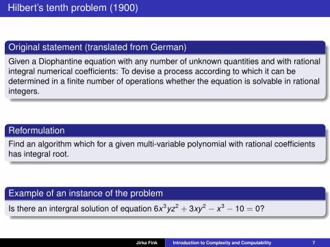
Original statement (translated from German)Given a Diophantine equation with any number of unknown quantities and with rationalintegral numerical coefficients: To devise a process according to which it can bedetermined in a finite number of operations whether the equation is solvable in rationalintegers.

ReformulationFind an algorithm which for a given multi-variable polynomial with rational coefficientshas integral root.

Example of an instance of the problem

Is there an intergral solution of equation 6x3yz2 + 3xy2 − x3 − 10 = 0?


Halting problem

Halting problemIs there an algorithm which for a given program and its input determines whether theprogram on that input terminates?

Example of a programint main(int argc, char *argv[]) int n, total, x, y, z;scanf("%d", &n);total=3;for(;;) for(x=1; x<=total-2; ++x) for(y=1; y<=total-x-1; ++y) z=total-x-y;if(exp(x,n)+exp(y,n)==exp(z,n))

return 0;

++total;


Random access machine

ComponentsMemory divided into cells

Cells are indexed by (positive) integersEvery cell can store a integer

Program composed of instructionsArithmetical instructions: additions, subtraction, multiplication, division, moduloLogical instructions: conjunction, disjunction, shiftControl instructions: conditional and unconditional jump, halt

Input and outputSpecial instruction for reading and writing, orstoring in memory in pre-defined cells

Special registers (e.g. program counter)

Arguments of instructions and memory indexingInteger, e.g. 3

Direct addressing, e.g. [4]

Indirect addressing, e.g. [[5]]

Example of instruction: [[5]] := 3 + [4]

Variables can be used to improve readability


Random access machine

Example: FactorialCalculate factorial of the input stored at [1] and save the results in [2].

[2] := 1loop:[2] := [1] * [2][1] := [1] - 1jump_if_positive [1], loophalt

Variants of Random access machinesMemory potentially infinite only in one direction

Cells with bounded number of bits

More instructions, e.g. function calls

More indirections in memory accessing

Etc.


Memory without random access (Source: Wikipedia)

Video Home System Compact Cassette

Memory access


Turing machine (Alan Turing, 1936)

DefinitionTuring machine is a quintuple (Q,Σ, δ, q0,F ) where

Q is a finite set of states (internal memory)Σ is a finite tape alphabet

i.e. every cell store one value from Σλ ∈ Σ represents an empty cell

δ : Q × Σ→ Q × Σ× R,N, L ∪ ⊥ is a transition function which for every stateof Q and every value in the current cell determines:

new state of internal memory,new value to be stored in the current cell,whether the head determining the current cell should be moved to right (R), left (L) orstay (N)⊥ represents termination

q0 ∈ Q is the initial state

F ⊆ Q is the set of accepting states


Turing machine

Configuration captures the full state of computation of a Turing machineA configuration is triple (q,m, h) where

q ∈ Q is the current state,

m ∈ ΣZ are symbols in all cells of the tape and

h ∈ Z is the index of the current cell (the position of head).

Initial configuration

The initial configuration is (q0,m, 0) where

q0 is the initial state and

m contains the input word surrounded by λ.


Turing machine

Single step of computation

Assume that the current configuration is (q,m, h) and δ(q,mh) = (q′, s, d) is result ofthe transition function. The new configuration after a single step of computation is(q′,m′, h′) where

m′i =

mi if i 6= hs if i = h

h′ =

h + 1 if d = Rh − 1 if d = Lh if d = N

TerminationThe computation terminates if δ(q,mh) = ⊥. The input word is accepted if q ∈ F ;otherwise, the word is rejected.


Turing machine

Possible results of computationsFor every Turing machine and its every input word, exactly one of the followingstatements holds:

Computation terminates and uses finitely many cells of the type.

Computation loops on finitely many configurations and finitely many cells are used.

Computation never terminates, never reaches the same configuration twice anduses infinitely many cells.

Variants of Turing machineTape potentially infinite only in one direction

Multiple tapes

Multiple heads on tapes

Non-deterministic Turing machines

All variants are equivalent to the basic model.


Turing machine → Random access machine

TheoremFor every Turing machine there exists an equivalent RAM.

ProofFor simplicity, consider one directional memory and tape

Represent states Q and tape alphabet Σ by integersMemory of RAM is organized as follows:

[0] : Position of head[1] : State q[2] and more : Content of the tape

Rewrite the transition function δ into instructions using “if-then-else” statements

Simulate the Turing machine on RAM


Random access machine → Turing machine

TheoremFor every Random access machine (RAM) there exists an equivalent Turing machine(TM).

ProofWe construct 4-tape TM:

Input tape: Sequence of numbers passed to RAM as the inpun written in binaryand separated with #

Output tape: TM writes here the numbers output by RAMMemory of RAM: Content of memory of RAM

The tape symbols are Σ = 0, 1,#, |, λIf the currently used cells are c1, c2, . . . , cm then the tape contains string:c1|[c1]#c2|[c2]# · · ·#cm|[cm]

Auxiliary tape: For computing addition, subtraction, indirect indices, copying partof the memory tape, etc

TM simulates every instruction of RAM as follows: 1

Copy arguments from the memory tape to the auxiliary tape

Evaluate the instruction on the auxiliary tape

Copy results to the memory tape


1 Program of a RAM consists of finitely many instructions and arguments (indices ofmemory cells) are bounded numbers. Therefore, the program can be “stored” in atransition functions δ and a program counter can be stored as a part of state spaceQ.


Words and languages

TerminologyAlphabet Σ is a finite set of characters (symbols)

Word is a finite sequece of characters over alphabet Σ

Σ? denotes the set of all words

Language L ⊆ Σ? is a set of words over alphabet Σ

Decision problemA decision problem is formalized as a question whether given word belongs to thelanguage.

NoteEvery language contains countably many words. The set of all decision problems isuncountable.


Turing decidable languages

TerminologyTM accept a word w ∈ Σ?, if computation of TM with input w terminates in anaccepting state

RAM accept a word w ∈ Σ?, if computation of RAM with input w outputs 1 andterminates

TM reject a word w ∈ Σ?, if computation of TM with input w terminates in annon-accepting state

RAM reject a word w ∈ Σ?, if computation of RAM with input w outputs 0terminates

The set of words accepted by TM M is a language denoted by L(M)

We denote the fact that computation of TM M on w terminates as M(w)↓(computation converges)

We denote the fact that computation of TM M on w does not terminate as M(w)↑(computation diverges)

Language L is partially (Turing) decidable (also recursively enumerable), if there isa TM M such that L = L(M)

Language L is (Turing) decidable (also recursive), if there is a TM M which alwaysterminates and L = L(M)


Numbering Turing machines

Numbering Random access machinesEvery program in C is a word over alpabet 0, 1, i.e. represented by an integer

Similarly, every RAM can be represented by an integer

Encode a Turing machine (Q,Σ, δ,q0,F ) as a word over a small alphabet Γ

Consider an alphabet Γ = 0, 1, L,N,R, |,#Encode every state Q and symbol Σ by a binary string

The set F is encoded as a concatenation of all states of F separated by |Instruction δ(q, s) = (q′, s′, d) is encoded as word q|s|q′|s′|d over 0, 1, |Function δ is encoded as a concatenation of all instructions separated with #

TU (Q,Σ, δ, q0,F ) is encoded as concatenation of q0, F and δ separated with #

Godel numberEncode every symbol of Γ by 3 bits (a word over 0, 1)Replace the word over Γ encoding TU by a word over 0, 1Precede the word over 0, 1 by the character 1 and read it as a binary integer

The resulting integer is called Godel number of a given Turing machine


Existence of an undecidable problems

Notes1 Some integers may not encode a valid Turing machine2 If M ∈ N is not a valid Turing machine, M(w) rejects every input w3 Integer representing a Turing machine is not unique4 For every decidable problem there exist infinitely many Turing machines deciding it5 There are only countably many Turing machines6 There are only countably many decidable languages

CorollaryThere exists an undecidable language.Furthermore, there are uncountably many undecidable languages.


Universal Turing machine

GoalCreate a Turing machine which for a given pair (M,w) computes the output of a Turingmachine M called on input w . 1

Universal TM has three memory types1st tape contains input, i.e. pair (M,w)

2nd tape contains binary encoded tape of M separated by |3rd tape contains binary encoded current state of M

Computation of Universal Turing machineCopy the input word w on the working (2nd) tape and set the initial state of M onthe 3rd tapeSimulates steps of M

Find the transition δ(q, s) = (q′, s′, d) on the 1st tape where q is the current state of Mstored on 3rd tape and s is the current symbol of M encoded on the current position on2nd tapeStore results q′ and s′ on the 3rd and 2nd tape and move 2nd head in direction d


1 We already proved that for every for every Random access machine R we canconstruct a Turing machine M which gives the same output for every input. Now,we create one Turing machine which simulates any TM/RAM.


Diagonalization (Cantor, 1873)

Observation

Let M be a set and 2M the set of all subsets of M (called a power set). Then, there isno surjection from M to 2M .

Proof

For a sake of contradiction, assume that there exists a surjection f : M → 2M

Let Z = a ∈ M; a 6∈ f (a)There exists x ∈ M such that f (x) = Z since f is a surjectionDoes x belong to Z? The following statements are equivalent:

x ∈ Zx 6∈ f (x) by definition of Zx 6∈ Z since f (x) = Z

Hence x ∈ Z ⇔ x 6∈ Z which is a contradition!


Halting problem

TheoremLet HALT be the set of all pairs (M,w) such that Turing machine M terminates on itsinput w . The language HALT is partially decidable but it is not decidable.

Proof (undecidability)For sake of a contradiction, assume that there exists a Turing machinehalting solver(M, w) which for a Turing machine M and an input w determineswhether M terminates on input w . 1 Consider the following adversary Turingmachine.

1 Program adversary(w)2 if halting solver(w,w) returns “Yes, it terminates” then3 Loop forever4 else5 Halt

The following statements are equivalent.

adversary(adversary) terminates

halting solver(adversary, adversary) returns “Yes, it terminates” 2

adversary(adversary) loops forever 3

This is a contradiction!Jirka Fink Introduction to Complexity and Computability 24

1 Keep in mind that inputs are represented as integers (or binary strings). Similarly,Turing machines are encoded as integers. Hence, integers represents inputs andalso Turing machines and we can use an input as a Turing machine and viceversa. For example, compilers expect programs as their inputs.

2 By definition of Turing machine halting solver.3 By definition of Turing machine adversary.


Undecidability of acceptance

TheoremLet ACCEPT be the set of all pairs (M,w) such that Turing machine M terminates andaccepts its input w . The language ACCEPT is partially decidable but it is not decidable.

Proof (undecidability)For sake of a contradiction, assume that there exists a Turing machineaccept solver(M, w) which for a Turing machine M and an input w determineswhether M terminates and accepts input w . Consider the following adversary Turingmachine.

1 Program adversary(w)2 if accept solver(w,w) accepts then3 return reject4 else5 return accept

The following statements are equivalent.

adversary(adversary) accepts

accept solver(adversary, adversary) accepts

adversary(adversary) rejects

This is a contradiction!Jirka Fink Introduction to Complexity and Computability 25

Undecidability of empty languages

TheoremLet EMPTY be the set of all Turing machines which does not accept any input. Thelanguage EMPTY undecidable.

Proof (undecidability)For sake of a contradiction, assume that there exists a Turing machineempty solver(M) which for a Turing machine M determines whether accept someinput. We construct Turing machine accept solver which is a contradiction.

1 Program accept solver(M, w)2 Program helper M (w)3 if w = M then4 return M(w)5 else6 return reject

7 if empty solver(helper M) accepts then8 return reject9 else

10 return accept


We prove that our accept solver works properly. First, consider a Turing machine Mwhich accept an input w which implies the following statements

helper M (M) accepts by definition of helper

L(helper M ) is non-empty is Turing machine helper M accepts input M

empty solver (helper M ) rejects

accept solver(M,w) accepts

Next, consider a Turing machine M which does not accept an input w which implies thefollowing statements

helper M does not accept any input

L(helper M ) is empty

empty solver (helper M ) accept

accept solver(M, w) rejects


Complement of languages

Definition

The complement of a language L ⊆ Σ? is the language L = Σ? \ L.

Observation

A language L is decidable if and only if the complement L is decidable.

Theorem (Post)

Language L is decidable if and only if languages L and L are partially decidable.

Corollary

Languages ACCEPT, HALT and EMPTY are not partially decidable.

ObservationIf L1 and L2 are (partially) decidable languages, then the following languages are also(partially) decidable.

L1 ∪ L2 1

L1 ∩ L2

L1 · L2 = ab; a ∈ L1, b ∈ L2, i.e. concatenation of words


1 If we have finitely many (partially) decidable languages L1, . . . , Lk , is the unionL1 ∪ · · · ∪ Lk (partially) decidable?If we have countably many (partially) decidable languages Li for i ∈ N, is the union⋃

i∈N Li (partially) decidable?


Turing computable functions

TerminologyIf a Turing machine M terminates on an input w then the output (content of thetape after computation) is denoted by fM (w).

Each Turing machine M with tape alphabet Σ computes some partial functionfM : Σ∗ 7→ Σ∗.

Function f : Σ∗ 7→ Σ∗ is Turing computable, if there is a Turing machine M whichcomputes it.

To each Turing computable function there is infinitely many Turing machinescomputing it!

NotesA program M (RAM/TM) which for an input x outputs y can be considered as afunction fM : Σ∗ 7→ Σ∗ such that fM (x) = y .

A function f : N→ N composed from some elementary (Turing computable)operations is a program which for an integer (word) x computes f (x).

Decidability of a language L ⊆ Σ? is a question whether the functionf : Σ? → 0, 1 is Turing computable where f (w) = 1 if and only w ∈ L.


Universal Turing machine, function, language

Universal Turing machineUniversal Turing machine computes for a given pair (M,w) the output of a Turingmachine M called on input w .

Universal functionA universal function Ψ satisfies Ψ(f , x) = f (x) for every partially computable function fand every argument of x of the domain of f .

Universal language

A universal language Lu is the set of pairs (M,w) such that Turing machine M acceptsw .

ObservationUniversal function Ψ is partially computable but it is not computable.Universal language Lu is partially decidable but it is not decidable.

ProofUse universal Turing machine . . .


Church-Turing thesis

IntuitivelyAn algorithm is a finite sequence of simple instructions which leads to a solution ofgiven problem.

Church-Turing thesisTo every algorithm in intuitive sense we can construct a Turing machine whichimplements it.

Equivalent computation modelsAccording to Church-Turing thesis, intuitive notion of algorithm is also equivalent with

description of a Turing machine,

program for RAM,

derivation of a partial recursive function,

derivation of a function in λ-calculus,

program in a programming language C, Pascal, Java, Basic, Lisp, Haskell etc.,

In all these models we can compute the same functions and solve the same problems.


Strings ordering

DefintionLet Σ be an alphabet and let us assume that < is a strict order over characters in Σ. Letu, v ∈ Σ? be two different strings. We say that u is lexicographically smaller than v if

u is shorter than v , or

u and v have the same length and if i is the first index with u[i] 6= v [i], thenu[i] < v [i].

This fact is denoted with u ≺ v . As usual we extend this notation to u v , u v andu v .

NoteLet u, v be words over 0, 1 and u′, v ′ ∈ N be the corresponding intergers (precededby “1”). Then u ≺ v if and only u′ < v ′.


Enumerator

DefinitionAn enumerator for a language L is a Turing machine E which

ignores its input,

during its computation writes words of L to a special output tape separated with‘#′, and

each string w ∈ L is eventually written by E .

If L is infinite, then E never stops.

Theorem1 A language L is partially decidable if and only if there is an enumerator E for L.2 An infinite language L is decidable if and only if there is an enumerator E for L

which outputs elements of L in lexicographic order.


Ideas of proofs:

Enumerator E for L⇒ L is partially decidable: Run the computation of enumeratorE and if it outputs a given word, then accept.

E enumerates in lexicographic order⇒ L is decidable: Run the computation ofenumerator E and if it outputs a given word w , then accept. If E outputs a wordlexicographically larger than w , then reject.

L is decidable⇒ E enumerates in lexicographic order: Decide all words one byone in lexicographic order.

L is partially decidable⇒ enumerator E for L: Decide all words “in parallel”.


Reducibility

DefinitionA language A ⊆ Σ? is m-reducible to a language B ⊆ Σ? if there exists acomputable function f : Σ? → Σ? such that w ∈ A⇔ f (w) ∈ B for every w ∈ Σ?.

A language A ⊆ Σ? is 1-reducible to a language B ⊆ Σ? if there exists acomputable injection f : Σ? → Σ? such that w ∈ A⇔ f (w) ∈ B for every w ∈ Σ?.

A language B is m-complete (1-complete) if B is partially decidable and anypartially decidable language A is m-reducible (1-reducible) to B.

Example (ACCEPT is m-reducible to HALT)For a Turing machine M and its input w , let f (M) be a Turing machine which calls M(w)and if M accepts w , then f (M) accepts w , otherwise M loops forever. 1

Theorem

If language A is m-reducible to a decidable language B, then A is decidable. 2

ExampleSince ACCEPT is reducible to HALT and ACCEPT is undecidable, HALT is alsoundecidable.


1 Informally, f is a program which obtains a source code of M and returns a sourcecode f (M) which differs from M by adding one if-then-else statement. Therefore, fonly trivially modify input source codes and it always terminates. The programf (M) loops if M loops or rejects. Since f is an injection, this is an example of1-reducibility.

2 For a given w ∈ Σ?, we compute f (w) and then use a Turing machine recognizingB to determine whether f (w) ∈ B.


S-m-n lemma

s-m-n lemma (computable function)For any two natural numbers m, n ≥ 1 there is a 1-1 total computable functionsm

n : Nm+1 7→ N such that for every x , y1, y2, . . . , ym, z1, . . . , zn ∈ Σ∗b :

ϕ(n)

smn (x,y1,y2,...,ym)

(z1, . . . , zn) ' ϕ(m+n)x (y1, . . . , ym, z1, . . . , zn)

s-m-n lemma (Informally)For all m, n ∈ N and every Turing machine M expecting input of length m + n and everyinput y1, . . . , ym there exists a Turing machine M ′ expecting input of length n such thatfor every input z1, . . . , zn computations M(y1, . . . , ym, z1, . . . , zn) and M ′(z1, . . . , zn) givethe same output. Furthermore, there exists a Turing machine SMN which for every Mand y1, . . . , ym computes M ′.

Pseudocode of SMN

1 Program SMN(M, y1, . . . , ym)2 Program M’(z1, . . . , zn)3 return M(y1, . . . , ym, z1, . . . , zn)

4 return M ′


Reducibility

ObservationsThe relation of m-reducibility is reflexive and transitive.

If m-complete language A is m-reducible to a partially decidable language B, thenB is m-complete.

TheoremThe following languages are m-complete.

ACCEPT = (M,w); M accepts wHALT = (M,w); M terminates on input wDIAG = M; Turing machine M terminates input word M

Proof (ACCEPT is m-complete)ACCEPT is a partially decidable language

We have to prove that for every Turing machine M there exists a computablefunction fM : Σ? → Σ? such that for every input w ∈ Σ? it holds that w ∈ L(M) ifand only if fM (w) ∈ ACCEPT

We have to find a computable function fM such that fM (w) = (M,w)

We use s-m-m lemma to “hard-code” M, so fM is SMN(Φ,M) where Φ is theuniversal TM.


Post correspondence problem (Post, 1946)

Input

Every domino contains two strings, one on each side; e.g. aab

An input to the problem is a collection of dominoes; e.g.

bca , a

ab , caa , abc

c

MatchA match a is a list of these dominoes (repetitions permitted) so that the string on the

top is the same as the string on the bottom; e.g. aab

bca

caa

aab

abcc

TheoremA problem whether for a given collection of dominoes there exists a match isundecidable.

ProofWe m-reduce ACCEPT language to the Post correspondence problem (language) asfollows.


Simplified Post correspondence problem

First, we consider the following simpler reductionConsider a one-directional Turing machine M = (Q,Σ, δ, q0,F ).

When M terminates, all cells of the tape store the empty symbol λ. 1

Assume that a match has to start with one given domino.

Terminology 2

A configuration of a M is a word over Q ∪ Σ obtained from the word stored on thetape by inserting the current state into the current position of head. 3

A history of computation is a concatenation all configurations separated with #and preceded and superseded #.

Our goal is to create a list of dominoes such that the matching word represents ahistory of computation.

The initial domino

##q0w1w2···wn#

where w1w2 · · ·wn is the input word. 4


1 Turing machine cleans up the tape before it terminates.2 We slightly modify few terms to simplify the proof.3 We assume that Q and Σ are disjoin. Formally, a configuration is a concatenation

of the following words:the content of the tape before the headthe current statethe symbol on the current position of headthe content of the tape after the head

Since Q ∩ Σ = ∅, the current state also indicates the current position of head ontape.

4 #q0w1w2 · · ·wn# is the initial configuration with separating symbols #.


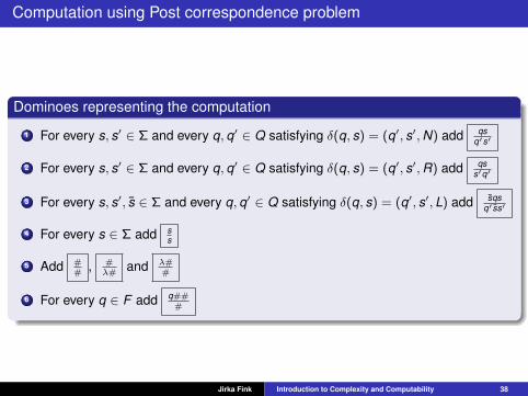
Computation using Post correspondence problem

Dominoes representing the computation

1 For every s, s′ ∈ Σ and every q, q′ ∈ Q satisfying δ(q, s) = (q′, s′,N) add qsq′s′

2 For every s, s′ ∈ Σ and every q, q′ ∈ Q satisfying δ(q, s) = (q′, s′,R) add qss′q′

3 For every s, s′, s ∈ Σ and every q, q′ ∈ Q satisfying δ(q, s) = (q′, s′, L) add sqsq′ ss′

4 For every s ∈ Σ add ss

5 Add ##

, #λ#

and λ##

6 For every q ∈ F add q###


Computation using Post correspondence problem

Reduction to the original Post corresponding problemFor a word w = w1w2 · · ·wn let

?w denotes ?w1 ? w2 ? · · · ? wn

w? denotes w1 ? w2 ? · · · ? wn?

?w? denotes ?w1 ? w2 ? · · · ? wn?

We reduce an instance of the Simplified Post corresponding problemt1b1

, t2b2

, . . . , tkbk

with the initial domino t1

b1

to an instance of the Post corresponding problem?t1?b1?

, ?t1b1?

, ?t2b2?

, . . . , ?tkbk?

, ?♥♥

.


Rice’s theorem

Rice’s theorem (languages)Let C be a class of partially decidable languages and let us defineLC = M; L(M) ∈ C. Then language LC is decidable if and only if C is either empty orit contains all partially decidable languages.

CorollaryThe following languages are undecidable.

Empty language: LC = M; L(M) = ∅ where C = ∅Finite languages: LC = M; L(M) is finite where C is the set of finite languages

Regular languages: LC = M; L(M) is regular where C is the set of regularlanguages

Decidable languages: LC = M; L(M) is decidable where C is the set ofdecidable languages

Rice’s theorem (functions)Let C be a class of computable functions and let us define AC = we; ϕe ∈ C. Thenlanguage AC is decidable if and only if C is either empty or it contains all computablefunctions.


Rice’s theorem

Rice’s theorem (languages)Let C be a class of partially decidable languages and let us defineLC = M; L(M) ∈ C. Then language LC is decidable if and only if C is either empty orit contains all partially decidable languages.

Proof (⇒)For sake of a contradiction, assume that C is decidable by a Turing machineC solver. WLOG: Turing machine Mreject rejecting all inputs does not belong to C andC contains a Turing machine Min. We construct Turing machine accept solverwhich is a contradiction.

1 Program accept solver(M, w)2 Program helper M,w (x)3 if M(w) accepts then4 Run Min(x) and return its output5 else6 Run Mreject (x) and return its output

7 Run C solver(helper M,w) and return its output


Note that C is decidable if and only if C is decidable. So, if Mreject ∈ C, we can considerC instead of C. We prove that our accept solver works properly. First, consider aTuring machine M which accept an input w which implies the following statements

helper M ,w(x) and Min(x) give the same output for all inputs x

L(helperM,w ) = L(Min)

C solver accepts both Min and helperM,w

accept solver(M,w) accepts

Next, consider a Turing machine M which does not accept an input w which implies thefollowing statements

both helper M,w and Mreject do not accect any word

L(helperM,w ) = L(Mreject )

C solver rejects both Mreject and helperM,w

accept solver(M,w) rejects


Outline

1 Computability

2 Complexity


Decision, search and optimization problem

Decision problemIn a decision problem we want to decide whether a given instance x satisfies aspecified condition.

Formalized as a language L ⊆ Σ∗ of positive instances and a decision whetherx ∈ L.

Search problemIn a search problem we aim to find for a given instance x an output y whichsatisfies a specified condition or information that no suitable y exists.

Formalized as a relation R ⊆ Σ∗ × Σ∗ which contains all pairs (x , y) satisfying aspecified condition.

Optimization problemIn an optimization problem we moreover require the output y to be maximal orminimal with respect to some measure.

Formalizad as a problem arg maxy∈Σ∗ f (x , y); (x , y) ∈ R where f is a (partial)ordering of all pairs (x , y).


Time and space complexity of a Turing machine

DefinitionLet M be (deterministic) Turing machine which halts on every input and let f : N 7→ Nbe a function.

We say that M runs in time f (n) if for any string x of length |x | = n the computationof M over x finishes within f (n) steps.

We say that M works in space f (n) if for any string x of length |x | = n thecomputation of M over x uses at most f (n) tape cells.

DefinitionLet f : N 7→ N be a function, then we define classes:

DTIME(f (n)) – class of languages which can be accepted by deterministic Turingmachines running in time O(f (n)).

DSPACE(f (n)) – class of languages which can be accepted by deterministic Turingmachines working in space O(f (n)).

ObservationDTIME(f (n)) ⊆ DSPACE(f (n)) for any function f : N 7→ N.


Important deterministic complexity classes

DefinitionClass of problems solvable in polynomial time:

P =⋃k∈N

DTIME(nk )

Class of problems solvable in polynomial space:

PSPACE =⋃k∈N

DSPACE(nk )

Class of problems solvable in exponential time:

EXP =⋃k∈N

DTIME(2nk)


Strong Church-Turing thesis

Strong Church-Turing thesisReal computation models can by simulated on TM with polynomial delay/spaceincrease.

NotesPolynomials are closed under composition.

Polynomial time algorithms are (usually) efficient in practice.

Definition of P does not depend on particular computational model we use (as faras it can be polynomially simulated on a TM).


Verifier

DefinitionA verifier for a language A is a Turing machine M, whereA = x ; ∃y : M accepts (x , y).

NotesA string y is called a certificate of x if M accepts (x , y).

Time and space complexities of a verifier is measured only in terms of |x |.Hence, if time or space complexity of a verifier is f (n), then the length of y is atmost f (n).

A polynomial time verifier runs in time polynomial in |x |.


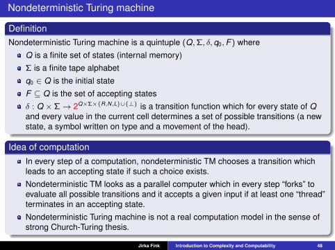
Nondeterministic Turing machine

DefinitionNondeterministic Turing machine is a quintuple (Q,Σ, δ, q0,F ) where

Q is a finite set of states (internal memory)

Σ is a finite tape alphabet

q0 ∈ Q is the initial state

F ⊆ Q is the set of accepting states

δ : Q × Σ→ 2Q×Σ×R,N,L∪⊥ is a transition function which for every state of Qand every value in the current cell determines a set of possible transitions (a newstate, a symbol written on type and a movement of the head).

Idea of computationIn every step of a computation, nondeterministic TM chooses a transition whichleads to an accepting state if such a choice exists.

Nondeterministic TM looks as a parallel computer which in every step “forks” toevaluate all possible transitions and it accepts a given input if at least one “thread”terminates in an accepting state.

Nondeterministic Turing machine is not a real computation model in the sense ofstrong Church-Turing thesis.


Nondeterministic Turing machine

DefinitionComputation of Nondeterministic TM M over string x is a sequence ofconfigurations C0,C1,C2, . . . , where

C0 is the initial configuration andCi+1 is obtained from Ci by applying one of possible transition defined by δ.

Computation is accepting if it is finite and M is in an accepting state in the lastconfiguration.

String x is accepted by NTM M if there is an accepting computation of M over x .

Language of string accepted by Nondeterministic TM M is denoted as L(M).

DefinitionLet M be a nondeterministic Turing machine and let f : N 7→ N be a function.

We say that M works in time f (n) if every computation of M over any input x oflength |x | = n terminates within f (n) steps.

We say that M works in space f (n) if every computation of M over any input x oflength |x | = n uses at most f (n) cells of work tape.


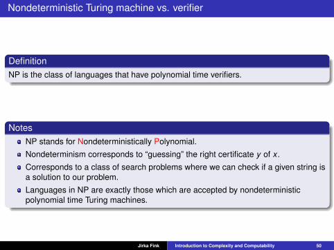
Nondeterministic Turing machine vs. verifier

DefinitionNP is the class of languages that have polynomial time verifiers.

NotesNP stands for Nondeterministically Polynomial.

Nondeterminism corresponds to “guessing” the right certificate y of x .

Corresponds to a class of search problems where we can check if a given string isa solution to our problem.

Languages in NP are exactly those which are accepted by nondeterministicpolynomial time Turing machines.


Basic nondeterministic complexity classes

DefinitionLet f : N 7→ N be a function, then we define classes:

NTIME(f (n)) – class of languages accepted by nondeterministic TMs working in timeO(f (n)).

NSPACE(f (n)) – class of languages accepted by nondeterministic TMs working inspace O(f (n)).

TheoremClass NP consists of languages accepted by nondeterministic Turing machinesworking in polynomial time, that is

NP =⋃k∈N

NTIME(nk ).

TheoremFor any function f : N 7→ N we have that

DTIME(f (n)) ⊆ NTIME(f (n)) ⊆ DSPACE(f (n)) ⊆ NSPACE(f (n)).


Turing machines using sublinear space

MotivationFormally, space complexity includes the size of input and output, although “workingspace” can be sublinear.

DefinitionIn case of sublinear space complexity, we use three tapes TM:

Read-only input tape

Write-only output tape (head moves only to the right)

Read-write working tapes

Only the working tape is included into space complexity.

DefinitionClass of problems solvable deterministically in logarithmic spaceL = DSPACE(log2 n).

Class of problems solvable nondeterministically in logarithmic spaceNL = NSPACE(log2 n).

Class of problems solvable nondeterministically in polynomial spaceNPSPACE =

⋃k∈N NSPACE(nk ).


Relations between classes

NotationLet f , g : N 7→ N. We say that f (n) = o(g(n)) if for every ε > 0 there exists n0 ∈ N suchthat for every n ≥ n0 it holds that f (n) < εg(n).Equivalently, f (n) = o(g(n)) if limn→∞

f (n)g(n)

= 0.

LemmaLet M be a deterministic or nondeterministic Turing machine working in space f (n).Then, there exists a constant cM such that the number all configurations of M is at most

2cM f (n) if f (n) = Ω(n)

n2cM f (n) if f (n) = o(n) using TM with sublinear space complexity. 1

TheoremLet f (n) be a function satisfying f (n) ≥ log2 n. For any language L ∈ NSPACE(f (n))there is a constant cL so that L ∈ TIME(2cLf (n)). 2

TheoremThe following chain of inclusions holds:

L ⊆ NL ⊆ P ⊆ NP ⊆ PSPACE ⊆ NPSPACE ⊆ EXP.


1 Number of possible contents on whole tape is |Σ|f (n).Number of positions of a head is f (n).Number of states is Q.

The total number of configurations is|Σ|f (n)f (n)Q = 2f (n) log |Σ|+log f (n)+log Q ≤ 2f (n)(log |Σ|+1+log Q) = 2cM f (n) wherecM = log |Σ|+ 1 + log Q.In the case of sublinear space complexity, we have to include the number ofpositions of a head on input tape, so the number of configurations is|Σ|f (n)f (n)Qn ≤ n2cM f (n).

2 Let M be a NTM deciding L in space f (n). We construct DTM M ′ deciding L intime 2cLf (n). M ′ constructs an oriented graph whose vertices are all configurationsof M and configuration C1 and C2 are connected by an edge if M switch from theconfiguration C1 to C2 in a single step. Then, M ′ determines whether there existsan oriented path from the initial configuration to an accepting configuration usingBFS or DFS.The number of vertices is at most n2cM f (n) and one vertex can be encoded inf (n) log |Σ|+ log Q + log f (n) + log n bits. The maximal out-degree of a vertex is23ΣQ . Hence, whole graph can be encoded in 2cG f (n) bits for some constant Gdepending on M only.TM can find a path in a graph in time O

(24cG f (n)

).


Savitch’s theorem

Theorem

For any function f (n) ≥ log2 n it holds that NSPACE(f (n)) ⊆ SPACE(f 2(n)).

Proof (using yieldability problem)

Given a NTM M working in space f (n), its two configuration C1 and C2 and t ∈ N, canM switch from the configuration C1 to C2 in at most t steps? 1

1 Program yield(C1, C2, t)2 if t = 1 then3 return accept if M can switch from C1 to C2 in a single step, otherwise reject4 else5 foreach configuration C′ do6 if both yield(C1, C′, bt/2c) and yield(C′, C2, dt/2e) accept then7 return accept

8 return reject

Corollary

PSPACE = NPSPACE


1 The initial configuration is known and the accepting configuration can be fixed bymodifying M so that tape is clear when M accepts.The running time of M is 2O(f (n)), so DTM accepts if yield(Cinit, Caccept, 2O(f (n)))accepts.Depth of the recursion is log 2O(f (n)) = O(f (n)).One configuration can be stored in O(f (n)) cells, so space complexity is O

(f 2(n)

).


Space hierarchy theorem

DefinitionA function f : N 7→ N, where f (n) ≥ log n, is called space constructible if the functionthat maps 1n to the binary representation of f (n) is computable in space O(f (n)).

Deterministic Space Hierarchy TheoremFor any space constructible function f : N 7→ N, there exists a language A that isdecidable in space O(f (n)) but not in space o(f (n)).

Corollary1 For any two functions f1, f2 : N 7→ N, where f1(n) ∈ o(f2(n)) and f2 is space

constructible,DSPACE(f1(n)) ( DSPACE(f2(n)).

2 For any two real numbers 0 ≤ a < b,

DSPACE(na) ( DSPACE(nb).

3 NL ( PSPACE ( EXPSPACE =⋃

k∈N DSPACE(2nk)




Idea of the proofCreate a TM D working in space O(f (n)) deciding a language denoted by A

Input is a word w of length n encoding a TM MMark space of length f (n) for simulation M(w)If simulation M(w) uses more that f (n) cells or loops, D rejectsD accepts w if and only if M rejects w

No TM M working in space o(f (n)) decides AFor constradiction, M decides A in space o(f (n)) and consider input w encoding MAssume D has enough space to simulate M(w)Then, M accepts w ⇔ D accepts w ⇔ M rejects w

Ensure that M has enough space to simulate M(w)D has a fixed tape alphabet simulating M with arbitrary tape alphabetIf M runs in space g(n), then D uses dg(n) spaceFrom g(n) ∈ o(f (n)) it follows that ∃n0 ∀n ≥ n0 : dg(n) < f (n)Let input word w be 〈M〉10n0 where 〈M〉 is the code of MThen |w | = n ≥ n0 and D can simulates M(w) in space f (n)

D must always terminate but M may loopIf M uses o(f (n)) space, then M uses 2o(f (n)) time or loopsD has a counter of steps of M and rejects if the counters exceeds 2f (n)




Algorithm D deciding some language A

1 Program D(w)2 Let n denotes the length of w3 Compute f (n) using space constructibility and mark off this much space4 if w is not of the form 〈M〉10n0 for some TM M then5 Reject

6 Simulates M on w :7 Count the number of steps and reject if the counter excedeeds 2f (n)

8 Reject if the simulation attempts to use more than f (n) space9 if M accepts w then

10 Reject11 else12 Accept


Time hierarchy theorem

DefinitionA function f : N 7→ N, where f (n) ≥ n log n, is called time constructible if the functionthat maps 1n to the binary representation of f (n) is computable in time O(f (n)).

Deterministic Time Hierarchy TheoremFor any time constructible function f : N 7→ N, there exists a language A that isdecidable in time O(f (n)) but not in time o(f (n)/ log f (n)).

Corollary1 For any two functions f1, f2 : N 7→ N, where f1(n) ∈ o(f2(n)/ log f2(n)) and f2 is time

constructible,DTIME(f1(n)) ( DTIME(f2(n)).

2 For any two real numbers 0 ≤ a < b,

DTIME(na) ( DTIME(nb).

3 P ( EXP


Time hierarchy theorem

Deterministic Time Hierarchy TheoremFor any time constructible function f : N 7→ N, there exists a language A that isdecidable in time O(f (n)) but not in time o(f (n)/ log f (n)).

Algorithm D deciding some language A

1 Program D(w)2 Let n denotes the length of w3 Compute f (n) using time constructibility and store it as a binary counter4 if w is not of the form 〈M〉10n0 for some TM M then5 Reject

6 Simulates M on w :7 Decrease the counter of steps and reject if the counter reaches 08 if M accepts w then9 Reject

10 else11 Accept


Polynomial reducibility

Definition

Language A is polynomially reducible to language B, denoted by A ≤Pm B, if there exists

a polynomial time computable function f : Σ∗ 7→ Σ∗ satisfying

(∀w ∈ Σ∗) [w ∈ A⇐⇒ f (w) ∈ B] .

Observation

≤Pm is reflexive and transitive relation (quasiorder).

If A ≤Pm B and B ∈ P then A ∈ P.

If A ≤Pm B and B ∈ NP then A ∈ NP.


NP-completeness

DefinitionLanguage B is NP-hard, if any language A ∈ NP is polynomially reducible to B.

Language B is NP-complete if B ∈ NP and B is NP-hard.

ObservationIf arbitrary NP-complete problem has polynomial time algorithm then P = NP.

If for language B it exists NP-complete problem A polynomially reducible to B (i.e.A ≤P

m B), then B is NP-hard.


NP-complete problem

TilingInstance: Set of colors B, natural number s, square grid S of size s × s, in which

border cells have outer edges colored by colors in B. Set of tile typesK , every tile is a square with edges colored by colors in B.

Question: Is there a valid tiling of S with tiles from K ? By a valid tiling we meanplacing tiles to cells of S without rotation, so that the tiles sharing aborder have matching color and the tiles placed in a border cell havethe colors matching outer edge colors of S.

TheoremTiling is NP-complete problem.

ObservationTiling is belongs to NP.


NP-hardness of Tiling

Every language A ∈ NP is polynomially reducible to Tiling

There exists NTM M deciding A in polynomial time p(n).For simplification we assume:

1 F = q1 where q1 6= q0, and δ(q1, a) = ∅ for every a ∈ Σ.2 Computation of M terminates with an empty tape (accepting configuration is unique).3 Tape is one-directional.

Let x be an instance of A and s = p(|x |).Rows encode configurations of computation of M:

The set of colors is Σ ∪ Q × (Σ ∪ L,R).Upper and bottom edges of the grid are colored by the initial and acceptingconfiguration, resp.Left and right edges of the grid are colored by λ.Types of tiles are defined by the transition function of M . . .

For every valid tiling there exists a computation of M.The sequence of colors between i-th and (i + 1)-th rows there exists exactly one colorfrom Q × Σ and other colors are from Q.


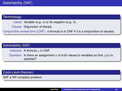
Satisfiability (SAT)

TerminologyLiteral: Variable (e.g. x) or its negation (e.g. x).

Clause: Disjunction of literals.

Conjunctive normal form (CNF): a formula is in CNF if it is a conjunction of clauses.

Satisfiability (SAT)Instance: A formula ϕ in CNF.

Question: Is there an assignment v of truth values to variables so that ϕ(v) issatisfied?

Cook-Levin theoremSAT is NP-complete problem.


Satisfiability (SAT)

SAT is NP-hard problem1 Given a set of colors B and types of tiles K and a grid s × s.2 Variables are xi,j,k for i , j = 1, . . . , s and k ∈ K .3 Assignment xi,j,k = 1 means that tiles of type K is places on position (i , j).4 Every position (i , j) has exactly one tile:∨

k∈K xi,j,kx i,j,k ∨ x i,j,k′ for every color k 6= k ′.

5 Colors are compatible between positions (i , j) a (i , j + 1):x i,j,k ∨ x i,j+1,k′ whenever the right edge of the tile k on position (i, j) differs from theleft edge of the tile k ′ on position (i, j + 1).

6 Color of upper edge of the grid is compatible with the first row:∨k∈Uj

x1,j,k where Uj is the set of tiles with upper edge colored by the same color asj-th column of the upper edge of the grid.

7 Similar clauses ensuring compatibility between position (i , j) and (i + 1, j) and alledge of the grid.

8 CNF ϕ is the conjunction of all presented clauses.


3-Satisfiability

DefinitionA formula ϕ is in k -CNF if it is in CNF and every clause consists of exactly k literalswhere k ∈ N.

k -SATInstance: A formula ϕ in k -CNF

Question: Is there an assignment v of truth values to variables so that ϕ(v) issatisfied?

Theorem

3-SAT is NP-complete problem. 1

Note2-SAT is polynomially solvable.


1 Too short clauses can be prolonged using additional variables, e.g. x1 ∨ x2 can bereplaced by (x1 ∨ x2 ∨ y)&(x1 ∨ x2 ∨ y). Too long clause x1 ∨ x2 ∨ x3 ∨ · · · ∨ xk canbe shortened by (x1 ∨ x2 ∨ y)&(y ∨ x3 ∨ · · · ∨ xk ) using additional variables.


Vertex Cover

Vertex Cover problemInstance: An undirected graph G = (V ,E) and an integer k ≥ 0.

Question: Is there a set of vertices S ⊆ V of size at most k so that each edgeu, v ∈ E has one of its endpoints in S (that is u, v ∩ S 6= ∅)?

Vertex cover problem is NP-completeWe construct a graph G for a given 3-SAT formula ϕ.

For every variable x in ϕ, add two vertices vx and vx joined by an edge.For every clause (e.g. x ∨ y ∨ z) in ϕ, add

three vertices cx , cy , and cz andedges cx cy , cx cz and cy cz (forming a triangle on cx , cy , and cz ) andedges cx vx , cy vy and czvz .

Let k = v + 2c where v and c is the number of variables and clauses, resp.

Observe that G has no vertex cover smaller than k .

G has a vertex cover of size k if and only if ϕ is satisfiable.


NP-complete problems related to Vertex Cover

CliqueInstance: An undirected graph G = (V ,E) and an integer k ≥ 0.

Question: Does G contain k vertices S such that every pair of vertices in S isconnected by an edge in G?

Independent setInstance: An undirected graph G = (V ,E) and an integer k ≥ 0.

Question: Does G contain k vertices S such that every pair of vertices in S is notconnected by an edge in G?

Edge cover

Instance: An undirected graph G = (V ,E) and an integer k ≥ 0.

Question: Does G contain k edges covering all vertices of G?


Hamiltonian cycle

Hamiltonian cycleInstance: An undirected graph G = (V ,E).

Question: Does G contain a cycle throught all vertices?

Travelling salesman problem, TSP

Instance: A complete graph G = (V ,E) with weights on edges w : E(G)→ Nand a limit d .

Question: Does G contain a Hamiltonian cycle with total weight at most d .

TheoremBoth Hamiltonain cycle and TSP are NP-complete problems.


3-Dimensional Matching

3-Dimensional MatchingInstance: Set M ⊆ W × X × Y , where W , X , and Y are sets of size q.

Question: Can we find a perfect matching in M? In particular, is there a setM ′ ⊆ M of size q so that all triples in M ′ are pairwise disjoint?

Theorem3-Dimensional Matching is an NP-complete problem.

TheoremExistence of a perfect matching in an undirected graph is polynomial problem.


Subset-Sum

Subset-SumInstance: Positive integers a1, . . . , ak and s which are binary coded.

Question: Is there a subset A ⊆ a1, . . . , ak such that∑

a∈A a = s?

Subset-Sum is NP-complete problem (reduction from 3-SAT)For a given 3-SAT ϕ on variables x1, . . . , xv and clauses c1, . . . , cd , we construct2(v + d) + 1 integers y1, . . . , yv , z1, . . . , zv , g1, . . . , gd , h1, . . . , hd , s, each one isv + d decimal integer of base 10 as follows.

1 Let yi [j] denotes j-th digit of integer yi .2 For a positive literal xi in a clause cj we set yi [j] = 1.3 For a negative literal xi in a clause cj we set zi [j] = 1.4 Let yi [d + i] = zi [d + i] = 1 for i = 1, . . . , v .5 Let yj [j] = zj [j] = 1 for j = 1, . . . , d .6 All other digits are 0.7 Let s[j] = 3 for j = 1, . . . , d and s[d + i] = 1 for i = 1, . . . , v .

There is no carry in the sum of all integers y1, . . . , hd in decimal representation.

In the subset A, we have to choose either yi or zi for every variable xi ⇒ yi ∈ A forpositive assignment of xi .

For every clause cj , at least one integer of y1, . . . , yv , z1, . . . , zv has to contribute by1 in the j-th digit to the sum

∑a∈A a⇒ at least one satisfied linteral in clause cj . 1


1 Observe that there a subset A of integers y1, . . . , hd with∑

a∈A a = s if and only ifϕ is satisfiable.


Subset-Sum

Subset-SumInstance: Positive integers a1, . . . , ak and s which are binary coded.

Question: Is there a subset A ⊆ a1, . . . , ak such that∑

a∈A a = s?

Subset-Sum is NP-complete if integers a1, . . . , ak and s are binary coded, but it ispolynomial if integers are unary coded.

Dynamic programming algorithm for Subset-Sum1 Consider logical variables zi,j which is true if there exists A ⊆ a1, . . . , ai such

that∑

a∈A = j for j = 0, . . . , s.2 Clearly, z0,0 is true and z0,j is false for j > 0.3 Observe that zi,j = zi−1,j ∨ zi−1,j−ai for i = 1, . . . , k and j = 0, . . . , s.4 Time complexity is O(ks) which is polynomial in the length of the input if all

integers a1, . . . , ak and s are unary coded.

3-partition is NP-complete even if integers are unary codedInstance: Positive integers a1, . . . , a3k .

Question: Can integers a1, . . . , a3k be split into k groups, each with 3 elements, sothat the sum of integers in each group is the same (i.e. 1

k

∑3ki=1 ai )?


Scheduling

Scheduling

Instance: A set of tasks U, processing time d(u) ∈ N associated with every tasku ∈ U, number of processors m, deadline D ∈ N

Question: Is it possible to assign all tasks to processors so that the (parallel)processing time is at most D?

TheoremScheduling is an NP-complete problem.


Number problem

DefinitionLet A be a decision problem and let I be an instance of A. Then

len(I) denotes the length (=number of bits) of encoding of I when using binaryencoding of numbers.

max(I) denotes the value of a maximum number parameter in I.

We say that A is a number problem, if for any polynomial p there is an instance I of Awith max(I) > p(len(I)).

ExamplesNumber problems : Subset-Sum, 3-partition, TSP

Non-number problems : Hamiltonicity, SAT


Pseudopolynomial algorithm

DefinitionWe say that an algorithm which solves problem A is pseudopolynomial if its runningtime is bounded by a polynomial in two variables len(I) and max(I).

NotesWe usually measure complexity of an algorithm only with respect to len(I).

If for some polynomial p and for every instance I of A we have thatmax(I) ≤ p(len(I)) then a pseudopolynomial algorithm is actually polynomial.

Also, if the numbers in I would be encoded in unary, a pseudopolynomial algorithmwould run in polynomial time.

For example, dynamic programming algorithm for Subset-Sum problem is apseudopolynomial.


Factorization

Trivial algorithm for factorization

Input: An integer n1 i := 22 while i · i ≤ n do3 if i divides n then

Output: i4 n := n/i5 else6 i := i + 1

7 if n > 1 thenOutput: n

Complexity

Complexity of the algorithm is O(√

n).

If a given integer n is encoded in unary, then√

n is a polynomial function, so thealgorithm is pseudopolynomial.

If a given integer n is encoded in binary using k = dlog ne bits, complexity isO(

2k/2)

which is exponential.


Strong NP-completeness

DefinitionLet A be a decision problem and let p be a polynomial. Then A(p) denotes therestriction of problem A to instances I which satisfy max(I) ≤ p(len(I)).

We say that problem A is strongly NP-complete, if there is a polynomial p for whichA(p) is NP-complete.

NotesAny NP-complete problem which is not a number problem is strongly NP-complete.

If there is a strongly NP-complete problem which can be solved by apseudopolynomial algorithm then P = NP.

Unary codingPseudopolynomial = polynomial when considering unary encoding.

Strongly NP-complete = NP-complete even when considering unary encoding.


Strong NP-completeness of number problems

”Weighted” versions of NP-complete problems”Weighted” versions of strongly NP-complete problems usually remain stronglyNP-complete, e.g.

Hamiltonicity→ Travelling Salesman problem

Vertex cover→ weighted vertex cover

Number problems3-partition: strongly NP-complete

Subset-Sum: NP-complete, pseudopolynomial algorithm

Factorization: pseudopolynomial algorithm

Prime testing: polynomial algorithm


Optimization problem

DefinitionWe define optimization problem as a triple A = (DA,SA, µA), where

DA ⊆ Σ∗ is a set of instances,

SA(I) assigns a set of feasible solutions to each I ∈ DA

µA(I, σ) assigns a positive rational value to every I ∈ DA and every feasiblesolution σ ∈ SA(I).

Optimum solutionIf A is a maximization problem, then an optimum solution to instance I is a feasiblesolution σ ∈ SA(I), which has the maximum value µA(I, σ).

If A is a minimization problem, then an optimum solution to instance I is a feasiblesolution σ ∈ SA(I), which has the minimum value µA(I, σ).

The value of an optimum solution is denoted opt(I).


Approximation algorithm for Vertex cover

Minimal vertex cover problemInstance: An undirected graph G = (V ,E).

Output: Find a vertex cover (i.e. S ⊆ V so that each edge u, v ∈ E has oneof its endpoints in S) with minimal size.

ObservationIf there exists a polynomial algorithm for minimal vertex cover problem, then P = NP.

Approximation algorithm

Input: Graph G1 Let M be a maximal matching of G2 Let S be the set of both endpoints of all edges of M

Output: S


Approximation algorithm for Vertex cover


Input: Graph G1 Let M be a maximal matching of G2 Let S be the set of both endpoints of all edges of M

Output: S

AnalysisThe running time is polynomialThe algorithm outputs a vertex cover

If there is an edge uv uncovered by S, then M ∪ uv is a matching, so M is not amaximal matching

If S′ is the minimal vertex cover, then |S| ≤ 2|S′|For every uv ∈ M, vertex u or v is covered by S′Hence, |S| = 2|M| ≤ 2|S′|



DefinitionAlgorithm R is called approximation algorithm for optimization problem A, if for eachinstance I ∈ A the output of R(I) is a feasible solution σ ∈ SA(I) (if there is any).

If A is a maximization problem, then c ≥ 1 is an approximation ratio of algorithmR, if for all instances I ∈ DA we have that opt(I) ≤ c · µA(I,R(I)).

If A is a minimization problem, then c ≥ 1 is an approximation ratio of algorithm R,if for all instances I ∈ DA we have that µA(I,R(I)) ≤ c · opt(I).

Example: Vertex cover

The algorithm finds a vertex cover S of size at most 2|S′| where S′ is the minimalvertex cover.

Therefore, the approximation ratio is 2.

Inapproximability of maximal independent setIf there exists a polynomial algorithm for maximal independent set with approximationerror c for some c > 1, then P= NP.


Travelling Salesman problem

TSP with triangular inequalityTSP is NP-complete even if weights of edges satisfies the triangular inequality.

Inapproximability of TSP (without triangular inequality)If for some c > 1 there exists a polynomial algorithm for TSP with approximation errorc, then P = NP.

Approximation of TSP with triangular inequalityFor TSP with triangular inequality there exists a polynomial algorithm withapproximation error 3/2.


Bin packing

Bin packing

Instance: Set of k items of rational sizes a1, . . . , ak ∈ [0, 1].

Constrain: Splitting of items to pairwise disjoint bins B1, . . . ,Bm, which satisfy thatthe sum of sizes of items in every bin is at most 1.

Objective: Minimize the number of bins m.

Any-Fit algorithmTake items as they come and for each item try to find a bin in which it fits. If no such binexists, add a new bin with the item in it.

Any-Fit algorithm has approximation error 2

The optimal number of bins m′ is at least∑k

i=1 ai .

For every pair of different bins Bi and Bj it holds that∑

l∈Bial +

∑l∈Bj

al > 1.

By summing last inequality for pairs (1, 2), (2, 3), . . . , (m − 1,m), (m, 1) we obtain2∑m

i=1

∑l∈Bi

l > m.

Hence, m < 2∑m

i=1

∑l∈Bi

l = 2∑k

i=1 ai ≤ 2m′.


Bin packing

Sorted-Any-Fit algorithmSort the items by their value decreasing. Take items from the biggest to smallest andfor each item try to find a bin in which it fits. If no such bin exists, add a new bin withthe item in it.

Best-fit algorithmTake items as they come and for each item try to find the most full bin in which it fits. Ifno such bin exists, add a new bin with the item in it.

NotesBest-fit algorithm has approximation error 1.7.

If m′ is the optimal number of bins and m is the number of bins found bySorted-Any-Fit algorithm, then m ≤ 11

9 m′ + 4.

There is no polynomial algorithm with approximation error smaller than 3/2.


Fully polynomial time approximation scheme

DefinitionsAlgorithm ALG is an approximation scheme for an optimization problem A, if onthe input instance I ∈ DA and a rational number ε it returns a solution σ ∈ SA(I)with approximation ratio 1 + ε.

If ALG works in polynomial time with respect to len(I), then it is a polynomial timeapproximation scheme.

If ALG works in polynomial time with respect to both len(I) and 1ε, it is a fully

polynomial time approximation schema (FPTAS).


Fully polynomial time approximation scheme

Optimization version of Subset-Sum problemInstance: Positive integers a1, . . . , ak and s which are binary coded.

Feasible solution: A subset A ⊆ a1, . . . , ak such that∑

a∈A a ≤ s.

Objective: Maximize∑

a∈A a.

Algorithm for the optimization version of Subset-sum

Input: Numbers a1, . . . , ak , s ∈ N and ε > 01 δ = k−1

√1

1+ε

2 A0 = 03 for i = 1 to k do4 Ai = Ai−1

5 for t ∈ Ai−1 do6 t ′ = t + ai

7 if t ′ ≤ s and Ai does not contain an integer between δt ′ and t ′ then8 Insert t ′ into Ai

9 return max Ak


Unsatisfiability

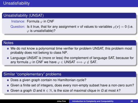
Unsatisfiability (UNSAT)Instance: Formula ϕ in CNF

Question: Is it true, that for any assignment v of values to variables ϕ(v) = 0 (i.e.ϕ is unsatisfiable)?

NotesWe do not know a polynomial time verifier for problem UNSAT, this problem mostprobably does not belong to class NP.

Language UNSAT is (more or less) the complement of language SAT, because forany formula ϕ in CNF we have ϕ ∈ UNSAT⇐⇒ ϕ /∈ SAT.

Similar “complementary” problemsDoes a given graph contain no Hamiltonian cycle?

Given a finite set of integers, does every non-empty subset have a non-zero sum?

Given a graph G and k ∈ N, is the size of maximal clique in G at most k?


Class coNP

Definition

We say that language A belongs to the class coNP if and only if its complement Abelongs to the class NP.

NotesFor instance UNSAT belongs to coNP. (It is easy to recognize instances which donot encode a formula.)

Language L belongs to coNP, iff there is a polynomial time verifier V whichsatisfies that L = x ; (∀y) V (x , y) accepts .Clearly, P ⊆ NP ∩ coNP.

It is not known whether NP = coNP.

Clearly, if P = NP, then NP = coNP.

A problem A is polynomially reducible to a problem B if and only if thecomplementary problem A is polynomially reducible to the complementaryproblem B.


coNP-completeness

DefinitionProblem A is coNP-complete, if

(i) A belongs to class coNP and

(ii) every problem B in coNP is polynomially reducible to A.

Notes

Language A is coNP-complete, if and only if complement A is NP-complete.

For example UNSAT is an coNP-complete problem.

If there is an NP-complete language A, which belongs to coNP, then NP = coNP.

Integer factorizationInstance: Positive integers m and n.

Question: Is there an integer k dividing m and satisfying 1 < k < n.

Clearly, Integer factorization belongs to NP.

Agrawal–Kayal–Saxena primality test implies that Integer factorization belongs tocoNP.

It is not known whether there exists a polynomial algorithm for Integer factorization.


Class #P

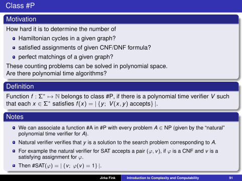
MotivationHow hard it is to determine the number of

Hamiltonian cycles in a given graph?

satisfied assignments of given CNF/DNF formula?

perfect matchings of a given graph?

These counting problems can be solved in polynomial space.Are there polynomial time algorithms?

DefinitionFunction f : Σ∗ 7→ N belongs to class #P, if there is a polynomial time verifier V suchthat each x ∈ Σ∗ satisfies f (x) = | y ; V (x , y) accepts |.

Notes

We can associate a function #A in #P with every problem A ∈ NP (given by the “natural”polynomial time verifier for A).

Natural verifier verifies that y is a solution to the search problem corresponding to A.

For example the natural verifier for SAT accepts a pair (ϕ, v), if ϕ is a CNF and v is asatisfying assignment for ϕ.

Then #SAT(ϕ) = | v ; ϕ(v) = 1 |.


Class #P (properties)

Nonzero value of f ∈ #PInstance: x ∈ Σ∗

Question: f (x) > 0?

NotesNonzero Value of f ∈ #P belongs to NP.

Value of f ∈ #P can be obtained by using polynomial number of queries about anelement belonging to the set (x ,N); f (x) ≥ N.Value of f ∈ #P can be computed in polynomial space.


Reducing a function to another function

DefinitionFunction f : Σ∗ 7→ N is polynomial reducible to function g : Σ∗ 7→ N if there arefunctions α : Σ∗ × N 7→ N and β : Σ∗ 7→ Σ∗, which can be computed in polynomial timeand

∀x ∈ Σ∗ : f (x) = α(x , g(β(x)))

NoteThis corresponds to the fact that f can be computed in polynomial time with one call offunction g (if this call is a constant time operation).


#P-completeness

DefinitionWe say that function f : Σ∗ 7→ N is #P-complete, if

(i) f ∈ #P and

(ii) every function g ∈ #P is polynomially reducible to f .

NotesFor example #SAT, #Vertex Cover and other counting versions of NP-completeproblems are #P-complete.

There are problems in P such that their counting versions are #P-complete.

Perfect matching in a bipartite graphsThe following problem is in P but it is #P-complete.

Instance: G = (A ∪ B,E) where E ⊆ A× B and A ∩ B = ∅ and |A| = |B|.Question: Is there a matching in G of size |A| = |B|?


Permanent of a matrix

DefinitionLet A be a matrix of type n × n. Then we define permanent of A as

perm(A) =∑π∈S(n)

n∏i=1

ai,π(i),

where S(n) is a set of permutations over set 1, . . . , n.

NotesLike “determinant” without a sign of permutation.

If A is a adjacency matrix of a bipartite graph G, then perm(A) computes thenumber of perfect matchings of G.

Function perm is #P-complete.


#DNF-SAT

#DNF-SATTerm is a conjunction of literals.

Disjunctive normal form (DNF) is a disjunction of terms.

Instance: Formula ϕ in DNF.

Question: Is there an assignment v such that ϕ(v) is satisfied?

This problem is in #P while it is decidable in polynomial time.


Parametrized version of Vertex Cover problem

Vertex Cover problemInstance: An undirected graph G = (V ,E) and an integer k ≥ 0.

Question: Is there a set of vertices S ⊆ V of size at most k so that each edgeu, v ∈ E has one of its endpoints in S?

This problem is strongly NP-complete. How the complexity depends on k?

Vertex Cover problem parametrized by the size k of a coverInstance: An undirected graph G = (V ,E).

Question: Is there a set of vertices S ⊆ V of size at most k so that each edgeu, v ∈ E has one of its endpoints in S?

Solvable by a brutal-force algorithm in time O(|V |k |E |

).

For every k ∈ N, this algorithm is polynomial although the degree of thepolynomial depends on k .


Fix-parameter tractability

Goal

Complexity of brutal-force algorithm for k -vertex cover problem is O(|V |k |E |

).

We would prefer a polynomial time algorithm for k -vertex cover such that thepolynomial is independent on k .

But there is no algorithm polynomial in both k and the size of input (unless P= NP).

We describe an algorithm running in time O(p(|V |)f (k)) where p is a polynomialfunction and f is an arbitrary function.


Fix-parameter tractability: Vertex Cover

Algorithm

1 Program Has Cover(Graph G, size of a vertex cover k)2 if G has no edge then3 return Accept

4 if k = 0 then5 return Reject

6 uv ← an arbitrary edge of G7 if Has Cover(G \ u, k − 1) or Has Cover(G \ v, k − 1) accepts then8 return Accept9 else

10 return Reject

ObservationsLet G be a graph and uv its edge and k ≥ 1. Then, G has a vertex cover of size kif and only if G \ u or G \ v has a vertex cover of size k − 1.

Time complexity is O(2k |V |

).


Fix-parameter tractability: Definitions

DefinitionsA parameter of a language L is a function k : Σ∗ → N.

A parametrized language is a language with a parameter.

A parameterized language is fix-parameter tractable (FPT) if there exists analgorithm A deciding L, a function f : N→ N and a polynomial function p : N→ Nsuch that A decides every instance x in time O(p(|x |) · f (k(x))).

NotesUsually, the parameter is a natural property of the problem and it may be a part ofthe input.

A language may have many interesting parametrizations.

ObservationA language L with a parameter k is fix-parameter tractable if and only if there exists analgorithm A′ deciding L, a function f ′ : N→ N and a polynomial function p′ : N→ Nsuch that A decides every instance x in time O(p′(|x |) + f ′(k(x))). 1


1 In proves of both implications, we can use the same algorithm and only determinefunctions giving complexity.⇒ Since ab ≤ a2b2 for a, b ≥ 0, it follows that p(|x |) · f (k(x)) ≤ p2(|x |) + f 2(k(x)).⇐ p′(|x |) + f ′(k(x)) ≤ 2p′(|x |) · f ′(k(x)) assuming p′(|x |), f ′(k(x)) ≥ 1.


Vertex Cover: Kernelization

Algorithm

Input: Graph G, size of a vertex cover k1 for every vertex v in G do2 if deg(v) > k then3 G← G \ v4 k ← k − 1

5 Remove all isolated vertices from G6 if k < 0 or |E | > k2 then7 return A canonical negative instance

8 return G, k

ObservationsLet v be a vertex of G of degree larger than k . Then G contains a vertex cover ofsize k if and only if G \ v contains a vertex cover of size k − 1.

If a graph of maximal degree k has a vertex cover of size k , then it has at most k2

edges.

The resulting graph contains at most k2 edges and 2k2 vertices.

Complexity is O(|V |+ |E |) and vertex cover can be found in O(|V |+ |E |+ k22k).


Kernelization

DefinitionA kernelization of a language L with a parameter k is a function g : Σ∗ → Σ∗ if

1 g computable in polynomial time and2 x ∈ L⇔ g(x) ∈ L for every x ∈ Σ∗ and3 there exists a function f : N→ N such that for every x ∈ Σ∗ it holds that|g(x)| ≤ f (k(x)).

TheoremA decidable parametrized language has a fix-parameter tractable if and only if it haskernelization.

Proof⇐: Run the kernelization and then the decider.⇒: Let A be an algorithm of running time O(p(|x |) · f (k(x))) and x be an instance.

If |x | ≤ f (k(x)), then x is already kernelized.If f (k(x)) ≤ |x |, then run A and return a canonical positive or negative instancedepending on whether x ∈ L. Running time is p(|x |) · f (k(x)) ≤ |x | · p(|x |).


introduction to complexity and computability -...

Documents