introduction to algorithms, 3rd ed. - mit press - massachusetts

Thomas H. CormenCharles E. LeisersonRonald L. RivestClifford Stein

Introduction to AlgorithmsThird Edition

The MIT PressCambridge, Massachusetts London, England

http://mitpress.mit.edu/0262533057

c� 2009 Massachusetts Institute of Technology

All rights reserved. No part of this book may be reproduced in any form or by any electronic or mechanical means(including photocopying, recording, or information storage and retrieval) without permission in writing from thepublisher.

For information about special quantity discounts, please email special [email protected].

This book was set in Times Roman and Mathtime Pro 2 by the authors.

Printed and bound in the United States of America.

Library of Congress Cataloging-in-Publication Data

Introduction to algorithms / Thomas H. Cormen . . . [et al.].—3rd ed.p. cm.

Includes bibliographical references and index.ISBN 978-0-262-03384-8 (hardcover : alk. paper)—ISBN 978-0-262-53305-8 (pbk. : alk. paper)1. Computer programming. 2. Computer algorithms. I. Cormen, Thomas H.

QA76.6.I5858 2009005.1—dc22

2009008593

10 9 8 7 6 5 4 3 2 1

27 Multithreaded Algorithms

The vast majority of algorithms in this book are serial algorithms suitable forrunning on a uniprocessor computer in which only one instruction executes at atime. In this chapter, we shall extend our algorithmic model to encompass parallelalgorithms, which can run on a multiprocessor computer that permits multipleinstructions to execute concurrently. In particular, we shall explore the elegantmodel of dynamic multithreaded algorithms, which are amenable to algorithmicdesign and analysis, as well as to efficient implementation in practice.

Parallel computers—computers with multiple processing units—have becomeincreasingly common, and they span a wide range of prices and performance. Rela-tively inexpensive desktop and laptop chip multiprocessors contain a single multi-core integrated-circuit chip that houses multiple processing “cores,” each of whichis a full-fledged processor that can access a common memory. At an intermedi-ate price/performance point are clusters built from individual computers—oftensimple PC-class machines—with a dedicated network interconnecting them. Thehighest-priced machines are supercomputers, which often use a combination ofcustom architectures and custom networks to deliver the highest performance interms of instructions executed per second.

Multiprocessor computers have been around, in one form or another, fordecades. Although the computing community settled on the random-access ma-chine model for serial computing early on in the history of computer science, nosingle model for parallel computing has gained as wide acceptance. A major rea-son is that vendors have not agreed on a single architectural model for parallelcomputers. For example, some parallel computers feature shared memory, whereeach processor can directly access any location of memory. Other parallel com-puters employ distributed memory, where each processor’s memory is private, andan explicit message must be sent between processors in order for one processor toaccess the memory of another. With the advent of multicore technology, however,every new laptop and desktop machine is now a shared-memory parallel computer,

Chapter 27 Multithreaded Algorithms 773

and the trend appears to be toward shared-memory multiprocessing. Although timewill tell, that is the approach we shall take in this chapter.

One common means of programming chip multiprocessors and other shared-memory parallel computers is by using static threading, which provides a softwareabstraction of “virtual processors,” or threads, sharing a common memory. Eachthread maintains an associated program counter and can execute code indepen-dently of the other threads. The operating system loads a thread onto a processorfor execution and switches it out when another thread needs to run. Although theoperating system allows programmers to create and destroy threads, these opera-tions are comparatively slow. Thus, for most applications, threads persist for theduration of a computation, which is why we call them “static.”

Unfortunately, programming a shared-memory parallel computer directly usingstatic threads is difficult and error-prone. One reason is that dynamically parti-tioning the work among the threads so that each thread receives approximatelythe same load turns out to be a complicated undertaking. For any but the sim-plest of applications, the programmer must use complex communication protocolsto implement a scheduler to load-balance the work. This state of affairs has ledtoward the creation of concurrency platforms, which provide a layer of softwarethat coordinates, schedules, and manages the parallel-computing resources. Someconcurrency platforms are built as runtime libraries, but others provide full-fledgedparallel languages with compiler and runtime support.

Dynamic multithreaded programming

One important class of concurrency platform is dynamic multithreading, which isthe model we shall adopt in this chapter. Dynamic multithreading allows program-mers to specify parallelism in applications without worrying about communicationprotocols, load balancing, and other vagaries of static-thread programming. Theconcurrency platform contains a scheduler, which load-balances the computationautomatically, thereby greatly simplifying the programmer’s chore. Although thefunctionality of dynamic-multithreading environments is still evolving, almost allsupport two features: nested parallelism and parallel loops. Nested parallelismallows a subroutine to be “spawned,” allowing the caller to proceed while thespawned subroutine is computing its result. A parallel loop is like an ordinaryfor loop, except that the iterations of the loop can execute concurrently.

These two features form the basis of the model for dynamic multithreading thatwe shall study in this chapter. A key aspect of this model is that the programmerneeds to specify only the logical parallelism within a computation, and the threadswithin the underlying concurrency platform schedule and load-balance the compu-tation among themselves. We shall investigate multithreaded algorithms written for

774 Chapter 27 Multithreaded Algorithms

this model, as well how the underlying concurrency platform can schedule compu-tations efficiently.

Our model for dynamic multithreading offers several important advantages:

� It is a simple extension of our serial programming model. We can describe amultithreaded algorithm by adding to our pseudocode just three “concurrency”keywords: parallel, spawn, and sync. Moreover, if we delete these concur-rency keywords from the multithreaded pseudocode, the resulting text is serialpseudocode for the same problem, which we call the “serialization” of the mul-tithreaded algorithm.

� It provides a theoretically clean way to quantify parallelism based on the no-tions of “work” and “span.”

� Many multithreaded algorithms involving nested parallelism follow naturallyfrom the divide-and-conquer paradigm. Moreover, just as serial divide-and-conquer algorithms lend themselves to analysis by solving recurrences, so domultithreaded algorithms.

� The model is faithful to how parallel-computing practice is evolving. A grow-ing number of concurrency platforms support one variant or another of dynamicmultithreading, including Cilk [51, 118], Cilk++ [72], OpenMP [60], Task Par-allel Library [230], and Threading Building Blocks [292].

Section 27.1 introduces the dynamic multithreading model and presents the met-rics of work, span, and parallelism, which we shall use to analyze multithreadedalgorithms. Section 27.2 investigates how to multiply matrices with multithread-ing, and Section 27.3 tackles the tougher problem of multithreading merge sort.

27.1 The basics of dynamic multithreading

We shall begin our exploration of dynamic multithreading using the example ofcomputing Fibonacci numbers recursively. Recall that the Fibonacci numbers aredefined by recurrence (3.22):

F0 D 0 ;

F1 D 1 ;

Fi D Fi�1 C Fi�2 for i � 2 :

Here is a simple, recursive, serial algorithm to compute the nth Fibonacci number:

27.1 The basics of dynamic multithreading 775

FIB.0/

FIB.0/FIB.0/FIB.0/

FIB.0/

FIB.1/FIB.1/

FIB.1/

FIB.1/

FIB.1/FIB.1/FIB.1/

FIB.1/

FIB.2/

FIB.2/FIB.2/FIB.2/

FIB.2/

FIB.3/FIB.3/

FIB.3/

FIB.4/

FIB.4/

FIB.5/

FIB.6/

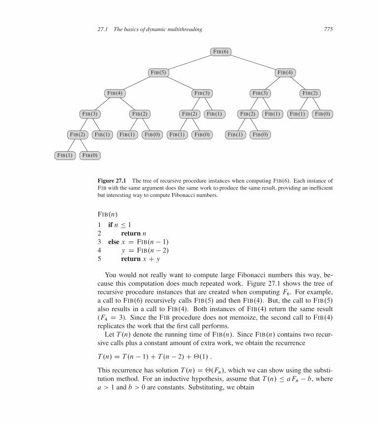
Figure 27.1 The tree of recursive procedure instances when computing FIB.6/. Each instance ofFIB with the same argument does the same work to produce the same result, providing an inefficientbut interesting way to compute Fibonacci numbers.

FIB.n/

1 if n � 1

2 return n

3 else x D FIB.n � 1/

4 y D FIB.n � 2/

5 return x C y

You would not really want to compute large Fibonacci numbers this way, be-cause this computation does much repeated work. Figure 27.1 shows the tree ofrecursive procedure instances that are created when computing F6. For example,a call to FIB.6/ recursively calls FIB.5/ and then FIB.4/. But, the call to FIB.5/

also results in a call to FIB.4/. Both instances of FIB.4/ return the same result(F4 D 3). Since the FIB procedure does not memoize, the second call to FIB.4/

replicates the work that the first call performs.Let T .n/ denote the running time of FIB.n/. Since FIB.n/ contains two recur-

sive calls plus a constant amount of extra work, we obtain the recurrence

T .n/ D T .n � 1/C T .n � 2/C‚.1/ :

This recurrence has solution T .n/ D ‚.Fn/, which we can show using the substi-tution method. For an inductive hypothesis, assume that T .n/ � aFn � b, wherea > 1 and b > 0 are constants. Substituting, we obtain


T .n/ � .aFn�1 � b/C .aFn�2 � b/C‚.1/

D a.Fn�1 C Fn�2/ � 2b C‚.1/

D aFn � b � .b �‚.1//

� aFn � b

if we choose b large enough to dominate the constant in the ‚.1/. We can thenchoose a large enough to satisfy the initial condition. The analytical bound

T .n/ D ‚.�n/ ; (27.1)

where � D .1 C p5/=2 is the golden ratio, now follows from equation (3.25).Since Fn grows exponentially in n, this procedure is a particularly slow way tocompute Fibonacci numbers. (See Problem 31-3 for much faster ways.)

Although the FIB procedure is a poor way to compute Fibonacci numbers, itmakes a good example for illustrating key concepts in the analysis of multithreadedalgorithms. Observe that within FIB.n/, the two recursive calls in lines 3 and 4 toFIB.n� 1/ and FIB.n� 2/, respectively, are independent of each other: they couldbe called in either order, and the computation performed by one in no way affectsthe other. Therefore, the two recursive calls can run in parallel.

We augment our pseudocode to indicate parallelism by adding the concurrencykeywords spawn and sync. Here is how we can rewrite the FIB procedure to usedynamic multithreading:

P-FIB.n/

1 if n � 1

2 return n

3 else x D spawn P-FIB.n � 1/

4 y D P-FIB.n � 2/

5 sync6 return x C y

Notice that if we delete the concurrency keywords spawn and sync from P-FIB,the resulting pseudocode text is identical to FIB (other than renaming the procedurein the header and in the two recursive calls). We define the serialization of a mul-tithreaded algorithm to be the serial algorithm that results from deleting the multi-threaded keywords: spawn, sync, and when we examine parallel loops, parallel.Indeed, our multithreaded pseudocode has the nice property that a serialization isalways ordinary serial pseudocode to solve the same problem.Nested parallelism occurs when the keyword spawn precedes a procedure call,

as in line 3. The semantics of a spawn differs from an ordinary procedure call inthat the procedure instance that executes the spawn—the parent—may continueto execute in parallel with the spawned subroutine—its child—instead of waiting


for the child to complete, as would normally happen in a serial execution. In thiscase, while the spawned child is computing P-FIB.n � 1/, the parent may go onto compute P-FIB.n � 2/ in line 4 in parallel with the spawned child. Since theP-FIB procedure is recursive, these two subroutine calls themselves create nestedparallelism, as do their children, thereby creating a potentially vast tree of subcom-putations, all executing in parallel.

The keyword spawn does not say, however, that a procedure must execute con-currently with its spawned children, only that it may. The concurrency keywordsexpress the logical parallelism of the computation, indicating which parts of thecomputation may proceed in parallel. At runtime, it is up to a scheduler to deter-mine which subcomputations actually run concurrently by assigning them to avail-able processors as the computation unfolds. We shall discuss the theory behindschedulers shortly.

A procedure cannot safely use the values returned by its spawned children untilafter it executes a sync statement, as in line 5. The keyword sync indicates thatthe procedure must wait as necessary for all its spawned children to complete be-fore proceeding to the statement after the sync. In the P-FIB procedure, a syncis required before the return statement in line 6 to avoid the anomaly that wouldoccur if x and y were summed before x was computed. In addition to explicitsynchronization provided by the sync statement, every procedure executes a syncimplicitly before it returns, thus ensuring that all its children terminate before itdoes.

A model for multithreaded execution

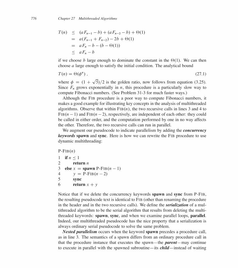
It helps to think of a multithreaded computation—the set of runtime instruc-tions executed by a processor on behalf of a multithreaded program—as a directedacyclic graph G D .V; E/, called a computation dag. As an example, Figure 27.2shows the computation dag that results from computing P-FIB.4/. Conceptually,the vertices in V are instructions, and the edges in E represent dependencies be-tween instructions, where .u; �/ 2 E means that instruction u must execute beforeinstruction �. For convenience, however, if a chain of instructions contains noparallel control (no spawn, sync, or return from a spawn—via either an explicitreturn statement or the return that happens implicitly upon reaching the end ofa procedure), we may group them into a single strand, each of which representsone or more instructions. Instructions involving parallel control are not includedin strands, but are represented in the structure of the dag. For example, if a strandhas two successors, one of them must have been spawned, and a strand with mul-tiple predecessors indicates the predecessors joined because of a sync statement.Thus, in the general case, the set V forms the set of strands, and the set E of di-rected edges represents dependencies between strands induced by parallel control.


P-FIB(1) P-FIB(0)

P-FIB(3)

P-FIB(4)

P-FIB(1)

P-FIB(1)

P-FIB(0)

P-FIB(2)

P-FIB(2)

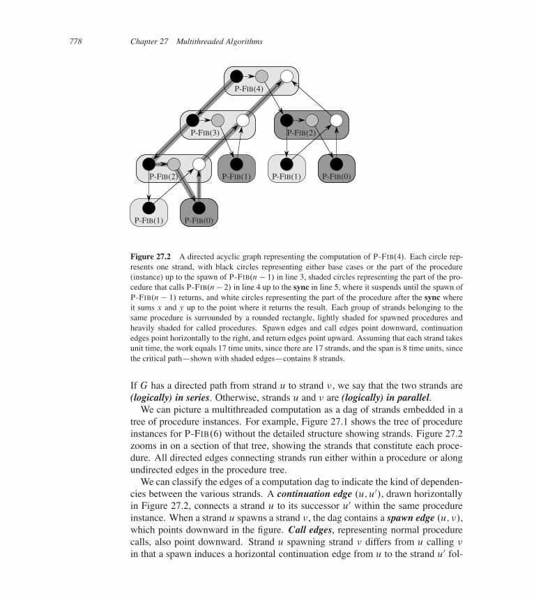
Figure 27.2 A directed acyclic graph representing the computation of P-FIB.4/. Each circle rep-resents one strand, with black circles representing either base cases or the part of the procedure(instance) up to the spawn of P-FIB.n � 1/ in line 3, shaded circles representing the part of the pro-cedure that calls P-FIB.n� 2/ in line 4 up to the sync in line 5, where it suspends until the spawn ofP-FIB.n � 1/ returns, and white circles representing the part of the procedure after the sync whereit sums x and y up to the point where it returns the result. Each group of strands belonging to thesame procedure is surrounded by a rounded rectangle, lightly shaded for spawned procedures andheavily shaded for called procedures. Spawn edges and call edges point downward, continuationedges point horizontally to the right, and return edges point upward. Assuming that each strand takesunit time, the work equals 17 time units, since there are 17 strands, and the span is 8 time units, sincethe critical path—shown with shaded edges—contains 8 strands.

If G has a directed path from strand u to strand �, we say that the two strands are(logically) in series. Otherwise, strands u and � are (logically) in parallel.

We can picture a multithreaded computation as a dag of strands embedded in atree of procedure instances. For example, Figure 27.1 shows the tree of procedureinstances for P-FIB.6/ without the detailed structure showing strands. Figure 27.2zooms in on a section of that tree, showing the strands that constitute each proce-dure. All directed edges connecting strands run either within a procedure or alongundirected edges in the procedure tree.

We can classify the edges of a computation dag to indicate the kind of dependen-cies between the various strands. A continuation edge .u; u0/, drawn horizontallyin Figure 27.2, connects a strand u to its successor u0 within the same procedureinstance. When a strand u spawns a strand �, the dag contains a spawn edge .u; �/,which points downward in the figure. Call edges, representing normal procedurecalls, also point downward. Strand u spawning strand � differs from u calling �

in that a spawn induces a horizontal continuation edge from u to the strand u0 fol-


lowing u in its procedure, indicating that u0 is free to execute at the same timeas �, whereas a call induces no such edge. When a strand u returns to its callingprocedure and x is the strand immediately following the next sync in the callingprocedure, the computation dag contains return edge .u; x/, which points upward.A computation starts with a single initial strand—the black vertex in the procedurelabeled P-FIB.4/ in Figure 27.2—and ends with a single final strand—the whitevertex in the procedure labeled P-FIB.4/.

We shall study the execution of multithreaded algorithms on an ideal paral-lel computer, which consists of a set of processors and a sequentially consistentshared memory. Sequential consistency means that the shared memory, which mayin reality be performing many loads and stores from the processors at the sametime, produces the same results as if at each step, exactly one instruction from oneof the processors is executed. That is, the memory behaves as if the instructionswere executed sequentially according to some global linear order that preserves theindividual orders in which each processor issues its own instructions. For dynamicmultithreaded computations, which are scheduled onto processors automaticallyby the concurrency platform, the shared memory behaves as if the multithreadedcomputation’s instructions were interleaved to produce a linear order that preservesthe partial order of the computation dag. Depending on scheduling, the orderingcould differ from one run of the program to another, but the behavior of any exe-cution can be understood by assuming that the instructions are executed in somelinear order consistent with the computation dag.

In addition to making assumptions about semantics, the ideal-parallel-computermodel makes some performance assumptions. Specifically, it assumes that eachprocessor in the machine has equal computing power, and it ignores the cost ofscheduling. Although this last assumption may sound optimistic, it turns out thatfor algorithms with sufficient “parallelism” (a term we shall define precisely in amoment), the overhead of scheduling is generally minimal in practice.

Performance measures

We can gauge the theoretical efficiency of a multithreaded algorithm by using twometrics: “work” and “span.” The work of a multithreaded computation is the totaltime to execute the entire computation on one processor. In other words, the workis the sum of the times taken by each of the strands. For a computation dag inwhich each strand takes unit time, the work is just the number of vertices in thedag. The span is the longest time to execute the strands along any path in the dag.Again, for a dag in which each strand takes unit time, the span equals the number ofvertices on a longest or critical path in the dag. (Recall from Section 24.2 that wecan find a critical path in a dag G D .V; E/ in ‚.V C E/ time.) For example, thecomputation dag of Figure 27.2 has 17 vertices in all and 8 vertices on its critical


path, so that if each strand takes unit time, its work is 17 time units and its spanis 8 time units.

The actual running time of a multithreaded computation depends not only onits work and its span, but also on how many processors are available and howthe scheduler allocates strands to processors. To denote the running time of amultithreaded computation on P processors, we shall subscript by P . For example,we might denote the running time of an algorithm on P processors by TP . Thework is the running time on a single processor, or T1. The span is the running timeif we could run each strand on its own processor—in other words, if we had anunlimited number of processors—and so we denote the span by T1.

The work and span provide lower bounds on the running time TP of a multi-threaded computation on P processors:

� In one step, an ideal parallel computer with P processors can do at most P

units of work, and thus in TP time, it can perform at most P TP work. Since thetotal work to do is T1, we have P TP � T1. Dividing by P yields the work law:

TP � T1=P : (27.2)

� A P -processor ideal parallel computer cannot run any faster than a machinewith an unlimited number of processors. Looked at another way, a machinewith an unlimited number of processors can emulate a P -processor machine byusing just P of its processors. Thus, the span law follows:

TP � T1 : (27.3)

We define the speedup of a computation on P processors by the ratio T1=TP ,which says how many times faster the computation is on P processors thanon 1 processor. By the work law, we have TP � T1=P , which implies thatT1=TP � P . Thus, the speedup on P processors can be at most P . When thespeedup is linear in the number of processors, that is, when T1=TP D ‚.P /, thecomputation exhibits linear speedup, and when T1=TP D P , we have perfectlinear speedup.

The ratio T1=T1 of the work to the span gives the parallelism of the multi-threaded computation. We can view the parallelism from three perspectives. As aratio, the parallelism denotes the average amount of work that can be performed inparallel for each step along the critical path. As an upper bound, the parallelismgives the maximum possible speedup that can be achieved on any number of pro-cessors. Finally, and perhaps most important, the parallelism provides a limit onthe possibility of attaining perfect linear speedup. Specifically, once the number ofprocessors exceeds the parallelism, the computation cannot possibly achieve per-fect linear speedup. To see this last point, suppose that P > T1=T1, in which case


the span law implies that the speedup satisfies T1=TP � T1=T1 < P . Moreover,if the number P of processors in the ideal parallel computer greatly exceeds theparallelism—that is, if P � T1=T1—then T1=TP � P , so that the speedup ismuch less than the number of processors. In other words, the more processors weuse beyond the parallelism, the less perfect the speedup.

As an example, consider the computation P-FIB.4/ in Figure 27.2, and assumethat each strand takes unit time. Since the work is T1 D 17 and the span is T1 D 8,the parallelism is T1=T1 D 17=8 D 2:125. Consequently, achieving much morethan double the speedup is impossible, no matter how many processors we em-ploy to execute the computation. For larger input sizes, however, we shall see thatP-FIB.n/ exhibits substantial parallelism.

We define the (parallel) slackness of a multithreaded computation executedon an ideal parallel computer with P processors to be the ratio .T1=T1/=P DT1=.P T1/, which is the factor by which the parallelism of the computation ex-ceeds the number of processors in the machine. Thus, if the slackness is less than 1,we cannot hope to achieve perfect linear speedup, because T1=.P T1/ < 1 and thespan law imply that the speedup on P processors satisfies T1=TP � T1=T1 < P .Indeed, as the slackness decreases from 1 toward 0, the speedup of the computationdiverges further and further from perfect linear speedup. If the slackness is greaterthan 1, however, the work per processor is the limiting constraint. As we shall see,as the slackness increases from 1, a good scheduler can achieve closer and closerto perfect linear speedup.

Scheduling

Good performance depends on more than just minimizing the work and span. Thestrands must also be scheduled efficiently onto the processors of the parallel ma-chine. Our multithreaded programming model provides no way to specify whichstrands to execute on which processors. Instead, we rely on the concurrency plat-form’s scheduler to map the dynamically unfolding computation to individual pro-cessors. In practice, the scheduler maps the strands to static threads, and the op-erating system schedules the threads on the processors themselves, but this extralevel of indirection is unnecessary for our understanding of scheduling. We canjust imagine that the concurrency platform’s scheduler maps strands to processorsdirectly.

A multithreaded scheduler must schedule the computation with no advanceknowledge of when strands will be spawned or when they will complete—it mustoperate on-line. Moreover, a good scheduler operates in a distributed fashion,where the threads implementing the scheduler cooperate to load-balance the com-putation. Provably good on-line, distributed schedulers exist, but analyzing themis complicated.


Instead, to keep our analysis simple, we shall investigate an on-line centralizedscheduler, which knows the global state of the computation at any given time. Inparticular, we shall analyze greedy schedulers, which assign as many strands toprocessors as possible in each time step. If at least P strands are ready to executeduring a time step, we say that the step is a complete step, and a greedy schedulerassigns any P of the ready strands to processors. Otherwise, fewer than P strandsare ready to execute, in which case we say that the step is an incomplete step, andthe scheduler assigns each ready strand to its own processor.

From the work law, the best running time we can hope for on P processorsis TP D T1=P , and from the span law the best we can hope for is TP D T1.The following theorem shows that greedy scheduling is provably good in that itachieves the sum of these two lower bounds as an upper bound.

Theorem 27.1On an ideal parallel computer with P processors, a greedy scheduler executes amultithreaded computation with work T1 and span T1 in time

TP � T1=P C T1 : (27.4)

Proof We start by considering the complete steps. In each complete step, theP processors together perform a total of P work. Suppose for the purpose ofcontradiction that the number of complete steps is strictly greater than bT1=P c.Then, the total work of the complete steps is at least

P � .bT1=P c C 1/ D P bT1=P c C P

D T1 � .T1 mod P /C P (by equation (3.8))

> T1 (by inequality (3.9)) .

Thus, we obtain the contradiction that the P processors would perform more workthan the computation requires, which allows us to conclude that the number ofcomplete steps is at most bT1=P c.

Now, consider an incomplete step. Let G be the dag representing the entirecomputation, and without loss of generality, assume that each strand takes unittime. (We can replace each longer strand by a chain of unit-time strands.) Let G0

be the subgraph of G that has yet to be executed at the start of the incomplete step,and let G00 be the subgraph remaining to be executed after the incomplete step. Alongest path in a dag must necessarily start at a vertex with in-degree 0. Since anincomplete step of a greedy scheduler executes all strands with in-degree 0 in G0,the length of a longest path in G00 must be 1 less than the length of a longest pathin G0. In other words, an incomplete step decreases the span of the unexecuted dagby 1. Hence, the number of incomplete steps is at most T1.

Since each step is either complete or incomplete, the theorem follows.


The following corollary to Theorem 27.1 shows that a greedy scheduler alwaysperforms well.

Corollary 27.2The running time TP of any multithreaded computation scheduled by a greedyscheduler on an ideal parallel computer with P processors is within a factor of 2

of optimal.

Proof Let T �P be the running time produced by an optimal scheduler on a machine

with P processors, and let T1 and T1 be the work and span of the computation,respectively. Since the work and span laws—inequalities (27.2) and (27.3)—giveus T �

P � max.T1=P; T1/, Theorem 27.1 implies that

TP � T1=P C T1� 2 �max.T1=P; T1/

� 2T �P :

The next corollary shows that, in fact, a greedy scheduler achieves near-perfectlinear speedup on any multithreaded computation as the slackness grows.

Corollary 27.3Let TP be the running time of a multithreaded computation produced by a greedyscheduler on an ideal parallel computer with P processors, and let T1 and T1 bethe work and span of the computation, respectively. Then, if P � T1=T1, wehave TP � T1=P , or equivalently, a speedup of approximately P .

Proof If we suppose that P � T1=T1, then we also have T1 � T1=P , andhence Theorem 27.1 gives us TP � T1=P C T1 � T1=P . Since the worklaw (27.2) dictates that TP � T1=P , we conclude that TP � T1=P , or equiva-lently, that the speedup is T1=TP � P .

The� symbol denotes “much less,” but how much is “much less”? As a ruleof thumb, a slackness of at least 10—that is, 10 times more parallelism than pro-cessors—generally suffices to achieve good speedup. Then, the span term in thegreedy bound, inequality 27.4, is less than 10% of the work-per-processor term,which is good enough for most engineering situations. For example, if a computa-tion runs on only 10 or 100 processors, it doesn’t make sense to value parallelismof, say 1,000,000 over parallelism of 10,000, even with the factor of 100 differ-ence. As Problem 27-2 shows, sometimes by reducing extreme parallelism, wecan obtain algorithms that are better with respect to other concerns and which stillscale up well on reasonable numbers of processors.


A

(a) (b)

B

A

B

Work: T1.A [ B/ D T1.A/C T1.B/

Span: T1.A[ B/ D T1.A/C T1.B/

Work: T1.A [ B/ D T1.A/C T1.B/

Span: T1.A [ B/ D max.T1.A/; T1.B/)

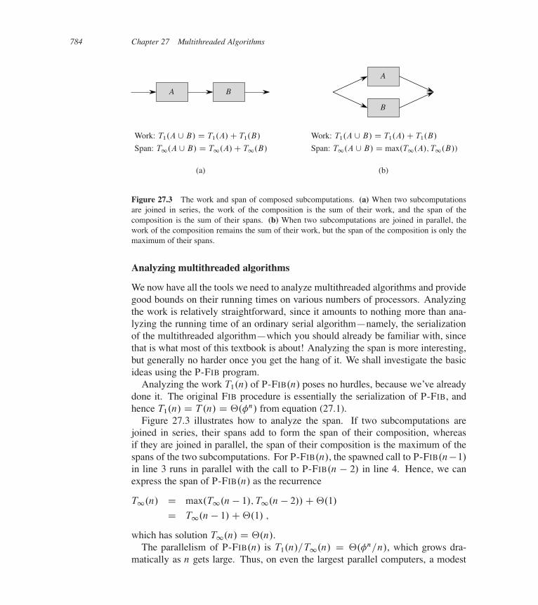
Figure 27.3 The work and span of composed subcomputations. (a) When two subcomputationsare joined in series, the work of the composition is the sum of their work, and the span of thecomposition is the sum of their spans. (b) When two subcomputations are joined in parallel, thework of the composition remains the sum of their work, but the span of the composition is only themaximum of their spans.

Analyzing multithreaded algorithms

We now have all the tools we need to analyze multithreaded algorithms and providegood bounds on their running times on various numbers of processors. Analyzingthe work is relatively straightforward, since it amounts to nothing more than ana-lyzing the running time of an ordinary serial algorithm—namely, the serializationof the multithreaded algorithm—which you should already be familiar with, sincethat is what most of this textbook is about! Analyzing the span is more interesting,but generally no harder once you get the hang of it. We shall investigate the basicideas using the P-FIB program.

Analyzing the work T1.n/ of P-FIB.n/ poses no hurdles, because we’ve alreadydone it. The original FIB procedure is essentially the serialization of P-FIB, andhence T1.n/ D T .n/ D ‚.�n/ from equation (27.1).

Figure 27.3 illustrates how to analyze the span. If two subcomputations arejoined in series, their spans add to form the span of their composition, whereasif they are joined in parallel, the span of their composition is the maximum of thespans of the two subcomputations. For P-FIB.n/, the spawned call to P-FIB.n�1/

in line 3 runs in parallel with the call to P-FIB.n � 2/ in line 4. Hence, we canexpress the span of P-FIB.n/ as the recurrence

T1.n/ D max.T1.n � 1/; T1.n � 2//C‚.1/

D T1.n � 1/C‚.1/ ;

which has solution T1.n/ D ‚.n/.The parallelism of P-FIB.n/ is T1.n/=T1.n/ D ‚.�n=n/, which grows dra-

matically as n gets large. Thus, on even the largest parallel computers, a modest


value for n suffices to achieve near perfect linear speedup for P-FIB.n/, becausethis procedure exhibits considerable parallel slackness.

Parallel loops

Many algorithms contain loops all of whose iterations can operate in parallel. Aswe shall see, we can parallelize such loops using the spawn and sync keywords,but it is much more convenient to specify directly that the iterations of such loopscan run concurrently. Our pseudocode provides this functionality via the parallelconcurrency keyword, which precedes the for keyword in a for loop statement.

As an example, consider the problem of multiplying an n n matrix A D .aij /

by an n-vector x D .xj /. The resulting n-vector y D .yi/ is given by the equation

yi DnX

j D1

aij xj ;

for i D 1; 2; : : : ; n. We can perform matrix-vector multiplication by computing allthe entries of y in parallel as follows:

MAT-VEC.A; x/

1 n D A:rows2 let y be a new vector of length n

3 parallel for i D 1 to n

4 yi D 0


6 for j D 1 to n

7 yi D yi C aij xj

8 return y

In this code, the parallel for keywords in lines 3 and 5 indicate that the itera-tions of the respective loops may be run concurrently. A compiler can implementeach parallel for loop as a divide-and-conquer subroutine using nested parallelism.For example, the parallel for loop in lines 5–7 can be implemented with the callMAT-VEC-MAIN-LOOP.A; x; y; n; 1; n/, where the compiler produces the auxil-iary subroutine MAT-VEC-MAIN-LOOP as follows:


1,1 2,2 3,3 4,4 5,5 6,6 7,7 8,8

1,2 3,4 5,6 7,8

1,4 5,8

1,8

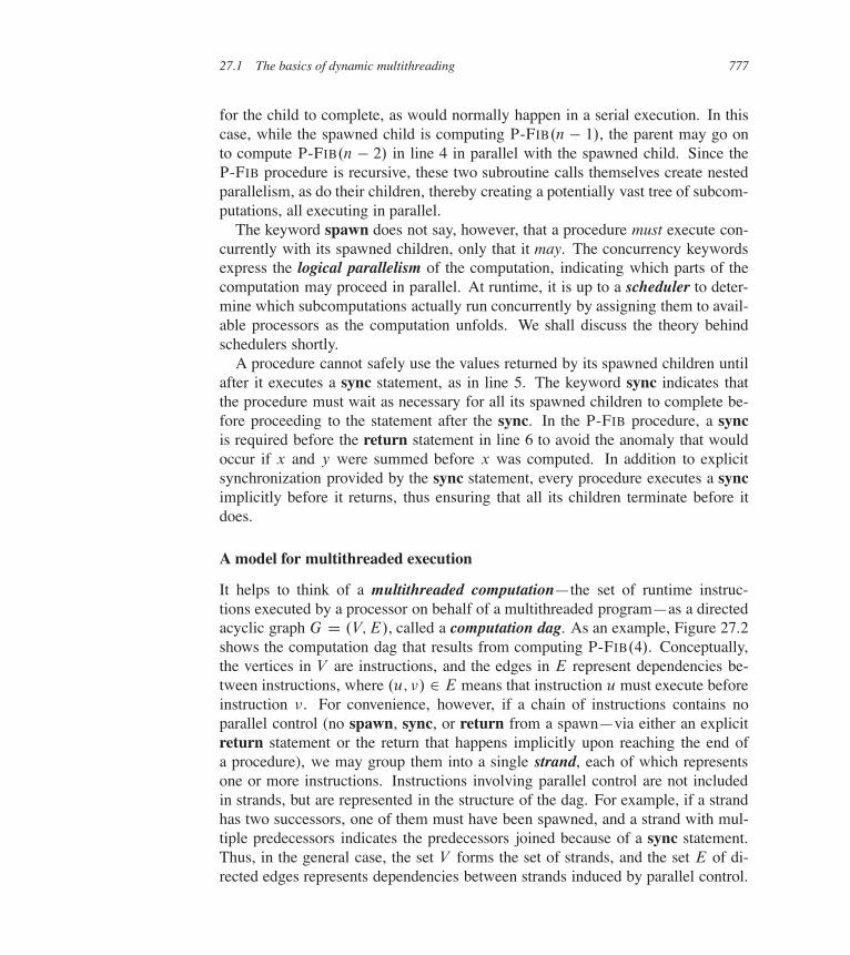
Figure 27.4 A dag representing the computation of MAT-VEC-MAIN-LOOP.A; x; y; 8; 1; 8/. Thetwo numbers within each rounded rectangle give the values of the last two parameters (i and i 0 inthe procedure header) in the invocation (spawn or call) of the procedure. The black circles repre-sent strands corresponding to either the base case or the part of the procedure up to the spawn ofMAT-VEC-MAIN-LOOP in line 5; the shaded circles represent strands corresponding to the part ofthe procedure that calls MAT-VEC-MAIN-LOOP in line 6 up to the sync in line 7, where it suspendsuntil the spawned subroutine in line 5 returns; and the white circles represent strands correspondingto the (negligible) part of the procedure after the sync up to the point where it returns.

MAT-VEC-MAIN-LOOP.A; x; y; n; i; i 0/

1 if i == i 0

2 for j D 1 to n

3 yi D yi C aij xj

4 else mid D b.i C i 0/=2c5 spawn MAT-VEC-MAIN-LOOP.A; x; y; n; i; mid/

6 MAT-VEC-MAIN-LOOP.A; x; y; n; midC 1; i 0/7 sync

This code recursively spawns the first half of the iterations of the loop to executein parallel with the second half of the iterations and then executes a sync, therebycreating a binary tree of execution where the leaves are individual loop iterations,as shown in Figure 27.4.

To calculate the work T1.n/ of MAT-VEC on an nn matrix, we simply computethe running time of its serialization, which we obtain by replacing the parallel forloops with ordinary for loops. Thus, we have T1.n/ D ‚.n2/, because the qua-dratic running time of the doubly nested loops in lines 5–7 dominates. This analysis


seems to ignore the overhead for recursive spawning in implementing the parallelloops, however. In fact, the overhead of recursive spawning does increase the workof a parallel loop compared with that of its serialization, but not asymptotically.To see why, observe that since the tree of recursive procedure instances is a fullbinary tree, the number of internal nodes is 1 fewer than the number of leaves (seeExercise B.5-3). Each internal node performs constant work to divide the iterationrange, and each leaf corresponds to an iteration of the loop, which takes at leastconstant time (‚.n/ time in this case). Thus, we can amortize the overhead of re-cursive spawning against the work of the iterations, contributing at most a constantfactor to the overall work.

As a practical matter, dynamic-multithreading concurrency platforms sometimescoarsen the leaves of the recursion by executing several iterations in a single leaf,either automatically or under programmer control, thereby reducing the overheadof recursive spawning. This reduced overhead comes at the expense of also reduc-ing the parallelism, however, but if the computation has sufficient parallel slack-ness, near-perfect linear speedup need not be sacrificed.

We must also account for the overhead of recursive spawning when analyzing thespan of a parallel-loop construct. Since the depth of recursive calling is logarithmicin the number of iterations, for a parallel loop with n iterations in which the i thiteration has span iter1.i/, the span is

T1.n/ D ‚.lg n/C max1�i�n

iter1.i/ :

For example, for MAT-VEC on an n n matrix, the parallel initialization loop inlines 3–4 has span ‚.lg n/, because the recursive spawning dominates the constant-time work of each iteration. The span of the doubly nested loops in lines 5–7is ‚.n/, because each iteration of the outer parallel for loop contains n iterationsof the inner (serial) for loop. The span of the remaining code in the procedureis constant, and thus the span is dominated by the doubly nested loops, yieldingan overall span of ‚.n/ for the whole procedure. Since the work is ‚.n2/, theparallelism is ‚.n2/=‚.n/ D ‚.n/. (Exercise 27.1-6 asks you to provide animplementation with even more parallelism.)

Race conditions

A multithreaded algorithm is deterministic if it always does the same thing on thesame input, no matter how the instructions are scheduled on the multicore com-puter. It is nondeterministic if its behavior might vary from run to run. Often, amultithreaded algorithm that is intended to be deterministic fails to be, because itcontains a “determinacy race.”

Race conditions are the bane of concurrency. Famous race bugs include theTherac-25 radiation therapy machine, which killed three people and injured sev-


eral others, and the North American Blackout of 2003, which left over 50 millionpeople without power. These pernicious bugs are notoriously hard to find. You canrun tests in the lab for days without a failure only to discover that your softwaresporadically crashes in the field.

A determinacy race occurs when two logically parallel instructions access thesame memory location and at least one of the instructions performs a write. Thefollowing procedure illustrates a race condition:

RACE-EXAMPLE. /

1 x D 0

2 parallel for i D 1 to 2

3 x D x C 1

4 print x

After initializing x to 0 in line 1, RACE-EXAMPLE creates two parallel strands,each of which increments x in line 3. Although it might seem that RACE-EXAMPLE should always print the value 2 (its serialization certainly does), it couldinstead print the value 1. Let’s see how this anomaly might occur.

When a processor increments x, the operation is not indivisible, but is composedof a sequence of instructions:

1. Read x from memory into one of the processor’s registers.

2. Increment the value in the register.

3. Write the value in the register back into x in memory.

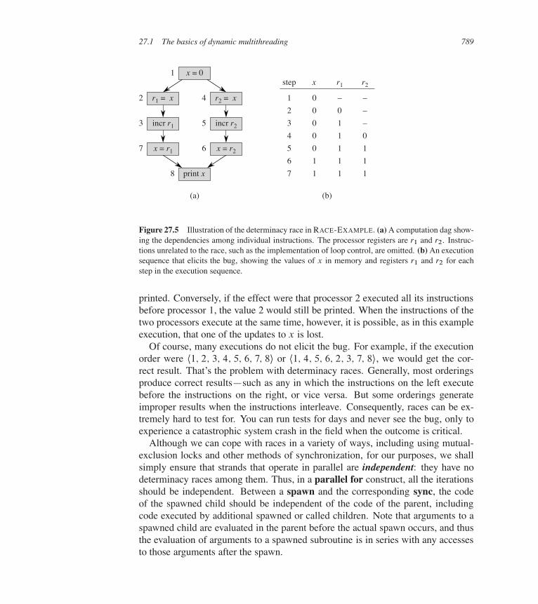
Figure 27.5(a) illustrates a computation dag representing the execution of RACE-EXAMPLE, with the strands broken down to individual instructions. Recall thatsince an ideal parallel computer supports sequential consistency, we can view theparallel execution of a multithreaded algorithm as an interleaving of instructionsthat respects the dependencies in the dag. Part (b) of the figure shows the valuesin an execution of the computation that elicits the anomaly. The value x is storedin memory, and r1 and r2 are processor registers. In step 1, one of the processorssets x to 0. In steps 2 and 3, processor 1 reads x from memory into its register r1

and increments it, producing the value 1 in r1. At that point, processor 2 comesinto the picture, executing instructions 4–6. Processor 2 reads x from memory intoregister r2; increments it, producing the value 1 in r2; and then stores this valueinto x, setting x to 1. Now, processor 1 resumes with step 7, storing the value 1

in r1 into x, which leaves the value of x unchanged. Therefore, step 8 prints thevalue 1, rather than 2, as the serialization would print.

We can see what has happened. If the effect of the parallel execution were thatprocessor 1 executed all its instructions before processor 2, the value 2 would be


incr r13

r1 = x2

x = r17

incr r25

r2 = x4

x = r26

x = 01

print x8

(a)

step x r1 r2

1

2

3

4

5

6

7

0

0

0

0

0

1

1

–

0

1

1

1

1

1

–

–

–

0

1

1

1

(b)

Figure 27.5 Illustration of the determinacy race in RACE-EXAMPLE. (a)A computation dag show-ing the dependencies among individual instructions. The processor registers are r1 and r2. Instruc-tions unrelated to the race, such as the implementation of loop control, are omitted. (b)An executionsequence that elicits the bug, showing the values of x in memory and registers r1 and r2 for eachstep in the execution sequence.

printed. Conversely, if the effect were that processor 2 executed all its instructionsbefore processor 1, the value 2 would still be printed. When the instructions of thetwo processors execute at the same time, however, it is possible, as in this exampleexecution, that one of the updates to x is lost.

Of course, many executions do not elicit the bug. For example, if the executionorder were h1; 2; 3; 4; 5; 6; 7; 8i or h1; 4; 5; 6; 2; 3; 7; 8i, we would get the cor-rect result. That’s the problem with determinacy races. Generally, most orderingsproduce correct results—such as any in which the instructions on the left executebefore the instructions on the right, or vice versa. But some orderings generateimproper results when the instructions interleave. Consequently, races can be ex-tremely hard to test for. You can run tests for days and never see the bug, only toexperience a catastrophic system crash in the field when the outcome is critical.

Although we can cope with races in a variety of ways, including using mutual-exclusion locks and other methods of synchronization, for our purposes, we shallsimply ensure that strands that operate in parallel are independent: they have nodeterminacy races among them. Thus, in a parallel for construct, all the iterationsshould be independent. Between a spawn and the corresponding sync, the codeof the spawned child should be independent of the code of the parent, includingcode executed by additional spawned or called children. Note that arguments to aspawned child are evaluated in the parent before the actual spawn occurs, and thusthe evaluation of arguments to a spawned subroutine is in series with any accessesto those arguments after the spawn.


As an example of how easy it is to generate code with races, here is a faultyimplementation of multithreaded matrix-vector multiplication that achieves a spanof ‚.lg n/ by parallelizing the inner for loop:

MAT-VEC-WRONG.A; x/

1 n D A:rows2 let y be a new vector of length n


4 yi D 0


6 parallel for j D 1 to n

7 yi D yi C aij xj

8 return y

This procedure is, unfortunately, incorrect due to races on updating yi in line 7,which executes concurrently for all n values of j . Exercise 27.1-6 asks you to givea correct implementation with ‚.lg n/ span.

A multithreaded algorithm with races can sometimes be correct. As an exam-ple, two parallel threads might store the same value into a shared variable, and itwouldn’t matter which stored the value first. Generally, however, we shall considercode with races to be illegal.

A chess lesson

We close this section with a true story that occurred during the development ofthe world-class multithreaded chess-playing program ?Socrates [81], although thetimings below have been simplified for exposition. The program was prototypedon a 32-processor computer but was ultimately to run on a supercomputer with 512

processors. At one point, the developers incorporated an optimization into the pro-gram that reduced its running time on an important benchmark on the 32-processormachine from T32 D 65 seconds to T 0

32 D 40 seconds. Yet, the developers usedthe work and span performance measures to conclude that the optimized version,which was faster on 32 processors, would actually be slower than the original ver-sion on 512 processsors. As a result, they abandoned the “optimization.”

Here is their analysis. The original version of the program had work T1 D 2048

seconds and span T1 D 1 second. If we treat inequality (27.4) as an equation,TP D T1=P C T1, and use it as an approximation to the running time on P pro-cessors, we see that indeed T32 D 2048=32 C 1 D 65. With the optimization, thework became T 0

1 D 1024 seconds and the span became T 01 D 8 seconds. Again

using our approximation, we get T 032 D 1024=32C 8 D 40.

The relative speeds of the two versions switch when we calculate the runningtimes on 512 processors, however. In particular, we have T512 D 2048=512C1 D 5


seconds, and T 0512 D 1024=512 C 8 D 10 seconds. The optimization that sped up

the program on 32 processors would have made the program twice as slow on 512

processors! The optimized version’s span of 8, which was not the dominant term inthe running time on 32 processors, became the dominant term on 512 processors,nullifying the advantage from using more processors.

The moral of the story is that work and span can provide a better means ofextrapolating performance than can measured running times.

Exercises

27.1-1Suppose that we spawn P-FIB.n � 2/ in line 4 of P-FIB, rather than calling itas is done in the code. What is the impact on the asymptotic work, span, andparallelism?

27.1-2Draw the computation dag that results from executing P-FIB.5/. Assuming thateach strand in the computation takes unit time, what are the work, span, and par-allelism of the computation? Show how to schedule the dag on 3 processors usinggreedy scheduling by labeling each strand with the time step in which it is executed.

27.1-3Prove that a greedy scheduler achieves the following time bound, which is slightlystronger than the bound proven in Theorem 27.1:

TP �T1 � T1

PC T1 : (27.5)

27.1-4Construct a computation dag for which one execution of a greedy scheduler cantake nearly twice the time of another execution of a greedy scheduler on the samenumber of processors. Describe how the two executions would proceed.

27.1-5Professor Karan measures her deterministic multithreaded algorithm on 4, 10,and 64 processors of an ideal parallel computer using a greedy scheduler. Sheclaims that the three runs yielded T4 D 80 seconds, T10 D 42 seconds, andT64 D 10 seconds. Argue that the professor is either lying or incompetent. (Hint:Use the work law (27.2), the span law (27.3), and inequality (27.5) from Exer-cise 27.1-3.)


27.1-6Give a multithreaded algorithm to multiply an n n matrix by an n-vector thatachieves ‚.n2= lg n/ parallelism while maintaining ‚.n2/ work.

27.1-7Consider the following multithreaded pseudocode for transposing an nn matrix A

in place:

P-TRANSPOSE.A/

1 n D A:rows2 parallel for j D 2 to n

3 parallel for i D 1 to j � 1

4 exchange aij with aj i

Analyze the work, span, and parallelism of this algorithm.

27.1-8Suppose that we replace the parallel for loop in line 3 of P-TRANSPOSE (see Ex-ercise 27.1-7) with an ordinary for loop. Analyze the work, span, and parallelismof the resulting algorithm.

27.1-9For how many processors do the two versions of the chess programs run equallyfast, assuming that TP D T1=P C T1?

27.2 Multithreaded matrix multiplication

In this section, we examine how to multithread matrix multiplication, a problemwhose serial running time we studied in Section 4.2. We’ll look at multithreadedalgorithms based on the standard triply nested loop, as well as divide-and-conqueralgorithms.

Multithreaded matrix multiplication

The first algorithm we study is the straighforward algorithm based on parallelizingthe loops in the procedure SQUARE-MATRIX-MULTIPLY on page 75:

27.2 Multithreaded matrix multiplication 793

P-SQUARE-MATRIX-MULTIPLY.A; B/

1 n D A:rows2 let C be a new n n matrix3 parallel for i D 1 to n


5 cij D 0

6 for k D 1 to n

7 cij D cij C aik � bkj

8 return C

To analyze this algorithm, observe that since the serialization of the algorithm isjust SQUARE-MATRIX-MULTIPLY, the work is therefore simply T1.n/ D ‚.n3/,the same as the running time of SQUARE-MATRIX-MULTIPLY. The span isT1.n/ D ‚.n/, because it follows a path down the tree of recursion for theparallel for loop starting in line 3, then down the tree of recursion for the parallelfor loop starting in line 4, and then executes all n iterations of the ordinary for loopstarting in line 6, resulting in a total span of ‚.lg n/ C ‚.lg n/ C ‚.n/ D ‚.n/.Thus, the parallelism is ‚.n3/=‚.n/ D ‚.n2/. Exercise 27.2-3 asks you to par-allelize the inner loop to obtain a parallelism of ‚.lg n/, which you cannot dostraightforwardly using parallel for, because you would create races.

A divide-and-conquer multithreaded algorithm for matrix multiplication

As we learned in Section 4.2, we can multiply n n matrices serially in time‚.nlg 7/ D O.n2:81/ using Strassen’s divide-and-conquer strategy, which motivatesus to look at multithreading such an algorithm. We begin, as we did in Section 4.2,with multithreading a simpler divide-and-conquer algorithm.

Recall from page 77 that the SQUARE-MATRIX-MULTIPLY-RECURSIVE proce-dure, which multiplies two n n matrices A and B to produce the n n matrix C ,relies on partitioning each of the three matrices into four n=2 n=2 submatrices:

A D�

A11 A12

A21 A22

�; B D

�B11 B12

B21 B22

�; C D

�C11 C12

C21 C22

�:

Then, we can write the matrix product as�C11 C12

C21 C22

�D

�A11 A12

A21 A22

��B11 B12

B21 B22

�D

�A11B11 A11B12

A21B11 A21B12

�C�

A12B21 A12B22

A22B21 A22B22

�: (27.6)

Thus, to multiply two nn matrices, we perform eight multiplications of n=2n=2

matrices and one addition of nn matrices. The following pseudocode implements


this divide-and-conquer strategy using nested parallelism. Unlike the SQUARE-MATRIX-MULTIPLY-RECURSIVE procedure on which it is based, P-MATRIX-MULTIPLY-RECURSIVE takes the output matrix as a parameter to avoid allocatingmatrices unnecessarily.

P-MATRIX-MULTIPLY-RECURSIVE.C; A; B/

1 n D A:rows2 if n == 1

3 c11 D a11b11

4 else let T be a new n n matrix5 partition A, B , C , and T into n=2 n=2 submatrices

A11; A12; A21; A22; B11; B12; B21; B22; C11; C12; C21; C22;and T11; T12; T21; T22; respectively

6 spawn P-MATRIX-MULTIPLY-RECURSIVE.C11; A11; B11/




10 spawn P-MATRIX-MULTIPLY-RECURSIVE.T11; A12; B21/



13 P-MATRIX-MULTIPLY-RECURSIVE.T22; A22; B22/

14 sync15 parallel for i D 1 to n


17 cij D cij C tij

Line 3 handles the base case, where we are multiplying 1 1 matrices. We handlethe recursive case in lines 4–17. We allocate a temporary matrix T in line 4, andline 5 partitions each of the matrices A, B , C , and T into n=2 n=2 submatrices.(As with SQUARE-MATRIX-MULTIPLY-RECURSIVE on page 77, we gloss overthe minor issue of how to use index calculations to represent submatrix sectionsof a matrix.) The recursive call in line 6 sets the submatrix C11 to the submatrixproduct A11B11, so that C11 equals the first of the two terms that form its sum inequation (27.6). Similarly, lines 7–9 set C12, C21, and C22 to the first of the twoterms that equal their sums in equation (27.6). Line 10 sets the submatrix T11 tothe submatrix product A12B21, so that T11 equals the second of the two terms thatform C11’s sum. Lines 11–13 set T12, T21, and T22 to the second of the two termsthat form the sums of C12, C21, and C22, respectively. The first seven recursivecalls are spawned, and the last one runs in the main strand. The sync statement inline 14 ensures that all the submatrix products in lines 6–13 have been computed,

27.2 Multithreaded matrix multiplication 795

after which we add the products from T into C in using the doubly nested parallelfor loops in lines 15–17.

We first analyze the work M1.n/ of the P-MATRIX-MULTIPLY-RECURSIVE

procedure, echoing the serial running-time analysis of its progenitor SQUARE-MATRIX-MULTIPLY-RECURSIVE. In the recursive case, we partition in ‚.1/ time,perform eight recursive multiplications of n=2 n=2 matrices, and finish up withthe ‚.n2/ work from adding two n n matrices. Thus, the recurrence for thework M1.n/ is

M1.n/ D 8M1.n=2/C‚.n2/

D ‚.n3/

by case 1 of the master theorem. In other words, the work of our multithreaded al-gorithm is asymptotically the same as the running time of the procedure SQUARE-MATRIX-MULTIPLY in Section 4.2, with its triply nested loops.

To determine the span M1.n/ of P-MATRIX-MULTIPLY-RECURSIVE, we firstobserve that the span for partitioning is ‚.1/, which is dominated by the ‚.lg n/

span of the doubly nested parallel for loops in lines 15–17. Because the eightparallel recursive calls all execute on matrices of the same size, the maximum spanfor any recursive call is just the span of any one. Hence, the recurrence for thespan M1.n/ of P-MATRIX-MULTIPLY-RECURSIVE is

M1.n/ DM1.n=2/C‚.lg n/ : (27.7)

This recurrence does not fall under any of the cases of the master theorem, butit does meet the condition of Exercise 4.6-2. By Exercise 4.6-2, therefore, thesolution to recurrence (27.7) is M1.n/ D ‚.lg2 n/.

Now that we know the work and span of P-MATRIX-MULTIPLY-RECURSIVE,we can compute its parallelism as M1.n/=M1.n/ D ‚.n3= lg2 n/, which is veryhigh.

Multithreading Strassen’s method

To multithread Strassen’s algorithm, we follow the same general outline as onpage 79, only using nested parallelism:

1. Divide the input matrices A and B and output matrix C into n=2 n=2 sub-matrices, as in equation (27.6). This step takes ‚.1/ work and span by indexcalculation.

2. Create 10 matrices S1; S2; : : : ; S10, each of which is n=2 n=2 and is the sumor difference of two matrices created in step 1. We can create all 10 matriceswith ‚.n2/ work and ‚.lg n/ span by using doubly nested parallel for loops.


3. Using the submatrices created in step 1 and the 10 matrices created instep 2, recursively spawn the computation of seven n=2 n=2 matrix productsP1; P2; : : : ; P7.

4. Compute the desired submatrices C11; C12; C21; C22 of the result matrix C byadding and subtracting various combinations of the Pi matrices, once againusing doubly nested parallel for loops. We can compute all four submatriceswith ‚.n2/ work and ‚.lg n/ span.

To analyze this algorithm, we first observe that since the serialization is thesame as the original serial algorithm, the work is just the running time of theserialization, namely, ‚.nlg 7/. As for P-MATRIX-MULTIPLY-RECURSIVE, wecan devise a recurrence for the span. In this case, seven recursive calls exe-cute in parallel, but since they all operate on matrices of the same size, we ob-tain the same recurrence (27.7) as we did for P-MATRIX-MULTIPLY-RECURSIVE,which has solution ‚.lg2 n/. Thus, the parallelism of multithreaded Strassen’smethod is ‚.nlg 7= lg2 n/, which is high, though slightly less than the parallelismof P-MATRIX-MULTIPLY-RECURSIVE.

Exercises

27.2-1Draw the computation dag for computing P-SQUARE-MATRIX-MULTIPLY on 22

matrices, labeling how the vertices in your diagram correspond to strands in theexecution of the algorithm. Use the convention that spawn and call edges pointdownward, continuation edges point horizontally to the right, and return edgespoint upward. Assuming that each strand takes unit time, analyze the work, span,and parallelism of this computation.

27.2-2Repeat Exercise 27.2-1 for P-MATRIX-MULTIPLY-RECURSIVE.

27.2-3Give pseudocode for a multithreaded algorithm that multiplies two n n matriceswith work ‚.n3/ but span only ‚.lg n/. Analyze your algorithm.

27.2-4Give pseudocode for an efficient multithreaded algorithm that multiplies a p q

matrix by a q r matrix. Your algorithm should be highly parallel even if any ofp, q, and r are 1. Analyze your algorithm.

27.3 Multithreaded merge sort 797

27.2-5Give pseudocode for an efficient multithreaded algorithm that transposes an n n

matrix in place by using divide-and-conquer to divide the matrix recursively intofour n=2 n=2 submatrices. Analyze your algorithm.

27.2-6Give pseudocode for an efficient multithreaded implementation of the Floyd-Warshall algorithm (see Section 25.2), which computes shortest paths between allpairs of vertices in an edge-weighted graph. Analyze your algorithm.

27.3 Multithreaded merge sort

We first saw serial merge sort in Section 2.3.1, and in Section 2.3.2 we analyzed itsrunning time and showed it to be ‚.n lg n/. Because merge sort already uses thedivide-and-conquer paradigm, it seems like a terrific candidate for multithreadingusing nested parallelism. We can easily modify the pseudocode so that the firstrecursive call is spawned:

MERGE-SORT0.A; p; r/

1 if p < r

2 q D b.p C r/=2c3 spawn MERGE-SORT 0.A; p; q/

4 MERGE-SORT 0.A; q C 1; r/

5 sync6 MERGE.A; p; q; r/

Like its serial counterpart, MERGE-SORT 0 sorts the subarray AŒp : : r�. After thetwo recursive subroutines in lines 3 and 4 have completed, which is ensured by thesync statement in line 5, MERGE-SORT 0 calls the same MERGE procedure as onpage 31.

Let us analyze MERGE-SORT 0. To do so, we first need to analyze MERGE. Re-call that its serial running time to merge n elements is ‚.n/. Because MERGE isserial, both its work and its span are ‚.n/. Thus, the following recurrence charac-terizes the work MS0

1.n/ of MERGE-SORT 0 on n elements:

MS01.n/ D 2 MS0

1.n=2/C‚.n/

D ‚.n lg n/ ;


… … …

… …merge mergecopy

p1 q1 r1 p2 q2 r2

p3 q3 r3

A

T

x

x

� x

� x < x

� x

� x � x

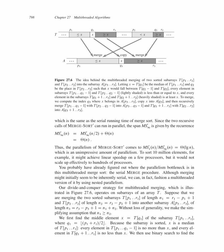
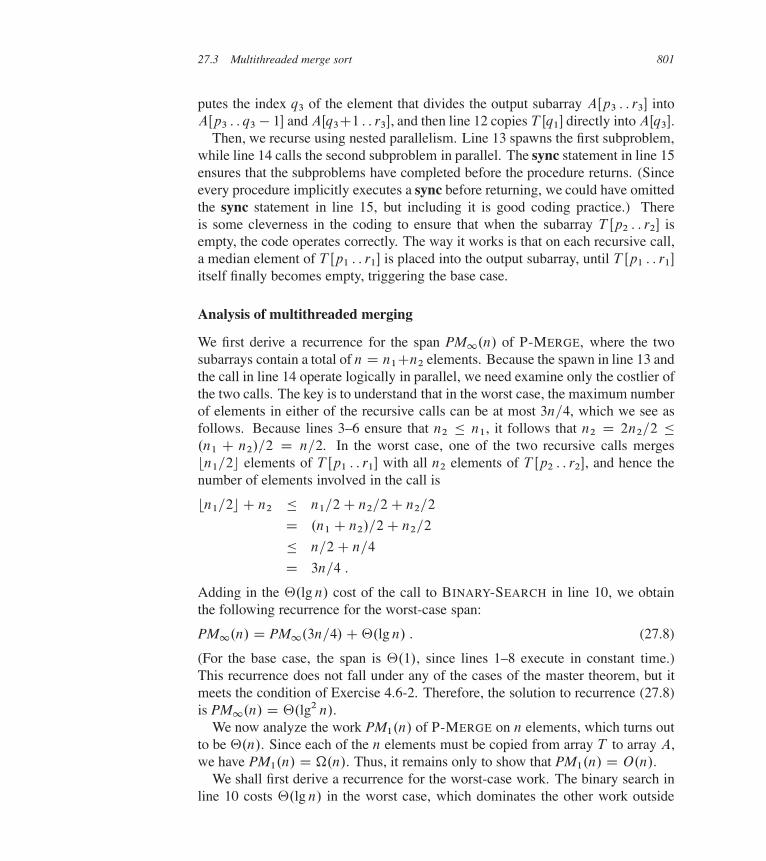
Figure 27.6 The idea behind the multithreaded merging of two sorted subarrays T Œp1 : : r1�

and T Œp2 : : r2� into the subarray AŒp3 : : r3�. Letting x D T Œq1� be the median of T Œp1 : : r1� and q2

be the place in T Œp2 : : r2� such that x would fall between T Œq2 � 1� and T Œq2�, every element insubarrays T Œp1 : : q1 � 1� and T Œp2 : : q2 � 1� (lightly shaded) is less than or equal to x, and everyelement in the subarrays T Œq1C 1 : : r1� and T Œq2C 1 : : r2� (heavily shaded) is at least x. To merge,we compute the index q3 where x belongs in AŒp3 : : r3�, copy x into AŒq3�, and then recursivelymerge T Œp1 : : q1 � 1� with T Œp2 : : q2 � 1� into AŒp3 : : q3 � 1� and T Œq1 C 1 : : r1� with T Œq2 : : r2�

into AŒq3 C 1 : : r3�.

which is the same as the serial running time of merge sort. Since the two recursivecalls of MERGE-SORT0 can run in parallel, the span MS0

1 is given by the recurrence

MS01.n/ D MS0

1.n=2/C‚.n/

D ‚.n/ :

Thus, the parallelism of MERGE-SORT0 comes to MS01.n/=MS0

1.n/ D ‚.lg n/,which is an unimpressive amount of parallelism. To sort 10 million elements, forexample, it might achieve linear speedup on a few processors, but it would notscale up effectively to hundreds of processors.

You probably have already figured out where the parallelism bottleneck is inthis multithreaded merge sort: the serial MERGE procedure. Although mergingmight initially seem to be inherently serial, we can, in fact, fashion a multithreadedversion of it by using nested parallelism.

Our divide-and-conquer strategy for multithreaded merging, which is illus-trated in Figure 27.6, operates on subarrays of an array T . Suppose that weare merging the two sorted subarrays T Œp1 : : r1� of length n1 D r1 � p1 C 1

and T Œp2 : : r2� of length n2 D r2 � p2 C 1 into another subarray AŒp3 : : r3�, oflength n3 D r3 � p3 C 1 D n1 C n2. Without loss of generality, we make the sim-plifying assumption that n1 � n2.

We first find the middle element x D T Œq1� of the subarray T Œp1 : : r1�,where q1 D b.p1 C r1/=2c. Because the subarray is sorted, x is a medianof T Œp1 : : r1�: every element in T Œp1 : : q1 � 1� is no more than x, and every el-ement in T Œq1 C 1 : : r1� is no less than x. We then use binary search to find the


index q2 in the subarray T Œp2 : : r2� so that the subarray would still be sorted if weinserted x between T Œq2 � 1� and T Œq2�.

We next merge the original subarrays T Œp1 : : r1� and T Œp2 : : r2� into AŒp3 : : r3�

as follows:

1. Set q3 D p3 C .q1 � p1/C .q2 � p2/.

2. Copy x into AŒq3�.

3. Recursively merge T Œp1 : : q1�1� with T Œp2 : : q2�1�, and place the result intothe subarray AŒp3 : : q3 � 1�.

4. Recursively merge T Œq1 C 1 : : r1� with T Œq2 : : r2�, and place the result into thesubarray AŒq3 C 1 : : r3�.

When we compute q3, the quantity q1�p1 is the number of elements in the subarrayT Œp1 : : q1 � 1�, and the quantity q2 � p2 is the number of elements in the subarrayT Œp2 : : q2 � 1�. Thus, their sum is the number of elements that end up before x inthe subarray AŒp3 : : r3�.

The base case occurs when n1 D n2 D 0, in which case we have no workto do to merge the two empty subarrays. Since we have assumed that the sub-array T Œp1 : : r1� is at least as long as T Œp2 : : r2�, that is, n1 � n2, we can checkfor the base case by just checking whether n1 D 0. We must also ensure that therecursion properly handles the case when only one of the two subarrays is empty,which, by our assumption that n1 � n2, must be the subarray T Œp2 : : r2�.

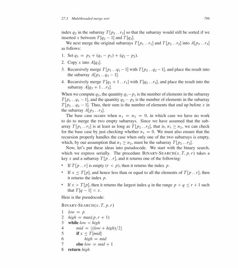
Now, let’s put these ideas into pseudocode. We start with the binary search,which we express serially. The procedure BINARY-SEARCH.x; T; p; r/ takes akey x and a subarray T Œp : : r�, and it returns one of the following:� If T Œp : : r� is empty (r < p), then it returns the index p.� If x � T Œp�, and hence less than or equal to all the elements of T Œp : : r�, then

it returns the index p.� If x > T Œp�, then it returns the largest index q in the range p < q � rC1 such

that T Œq � 1� < x.

Here is the pseudocode:

BINARY-SEARCH.x; T; p; r/

1 low D p

2 high D max.p; r C 1/

3 while low < high4 mid D b.lowC high/=2c5 if x � T Œmid�

6 high D mid7 else low D midC 1

8 return high


The call BINARY-SEARCH.x; T; p; r/ takes ‚.lg n/ serial time in the worst case,where n D r � p C 1 is the size of the subarray on which it runs. (See Exer-cise 2.3-5.) Since BINARY-SEARCH is a serial procedure, its worst-case work andspan are both ‚.lg n/.

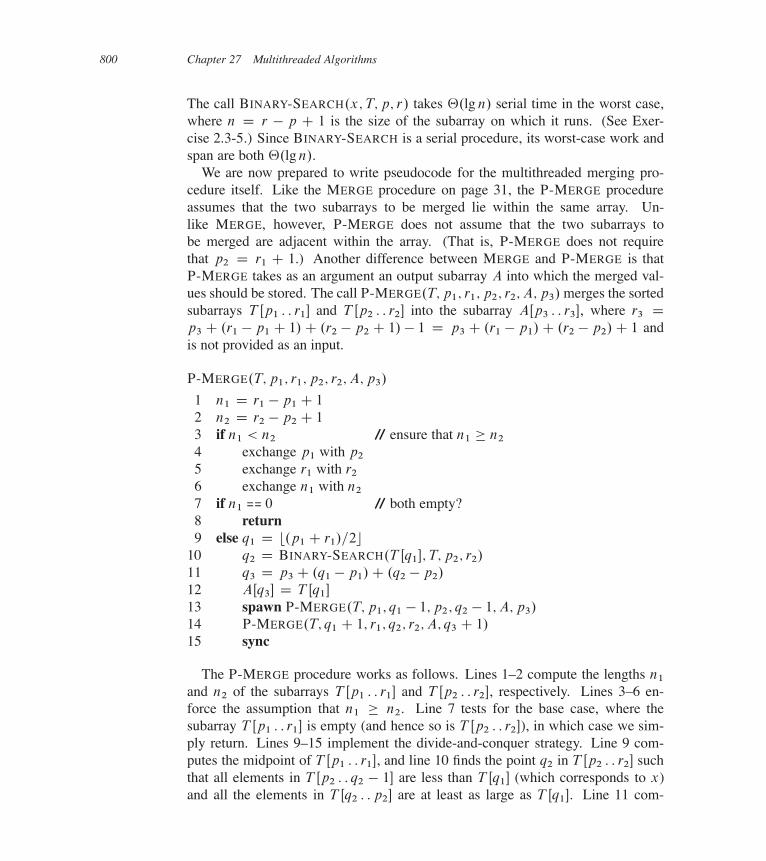
We are now prepared to write pseudocode for the multithreaded merging pro-cedure itself. Like the MERGE procedure on page 31, the P-MERGE procedureassumes that the two subarrays to be merged lie within the same array. Un-like MERGE, however, P-MERGE does not assume that the two subarrays tobe merged are adjacent within the array. (That is, P-MERGE does not requirethat p2 D r1 C 1.) Another difference between MERGE and P-MERGE is thatP-MERGE takes as an argument an output subarray A into which the merged val-ues should be stored. The call P-MERGE.T; p1; r1; p2; r2; A; p3/ merges the sortedsubarrays T Œp1 : : r1� and T Œp2 : : r2� into the subarray AŒp3 : : r3�, where r3 Dp3 C .r1 � p1 C 1/C .r2 � p2 C 1/ � 1 D p3 C .r1 � p1/C .r2 � p2/C 1 andis not provided as an input.

P-MERGE.T; p1; r1; p2; r2; A; p3/

1 n1 D r1 � p1 C 1

2 n2 D r2 � p2 C 1

3 if n1 < n2 // ensure that n1 � n2

4 exchange p1 with p2

5 exchange r1 with r2

6 exchange n1 with n2

7 if n1 == 0 // both empty?8 return9 else q1 D b.p1 C r1/=2c

10 q2 D BINARY-SEARCH.T Œq1�; T; p2; r2/

11 q3 D p3 C .q1 � p1/C .q2 � p2/

12 AŒq3� D T Œq1�

13 spawn P-MERGE.T; p1; q1 � 1; p2; q2 � 1; A; p3/

14 P-MERGE.T; q1 C 1; r1; q2; r2; A; q3 C 1/

15 sync

The P-MERGE procedure works as follows. Lines 1–2 compute the lengths n1

and n2 of the subarrays T Œp1 : : r1� and T Œp2 : : r2�, respectively. Lines 3–6 en-force the assumption that n1 � n2. Line 7 tests for the base case, where thesubarray T Œp1 : : r1� is empty (and hence so is T Œp2 : : r2�), in which case we sim-ply return. Lines 9–15 implement the divide-and-conquer strategy. Line 9 com-putes the midpoint of T Œp1 : : r1�, and line 10 finds the point q2 in T Œp2 : : r2� suchthat all elements in T Œp2 : : q2 � 1� are less than T Œq1� (which corresponds to x)and all the elements in T Œq2 : : p2� are at least as large as T Œq1�. Line 11 com-


putes the index q3 of the element that divides the output subarray AŒp3 : : r3� intoAŒp3 : : q3 � 1� and AŒq3C1 : : r3�, and then line 12 copies T Œq1� directly into AŒq3�.

Then, we recurse using nested parallelism. Line 13 spawns the first subproblem,while line 14 calls the second subproblem in parallel. The sync statement in line 15ensures that the subproblems have completed before the procedure returns. (Sinceevery procedure implicitly executes a sync before returning, we could have omittedthe sync statement in line 15, but including it is good coding practice.) Thereis some cleverness in the coding to ensure that when the subarray T Œp2 : : r2� isempty, the code operates correctly. The way it works is that on each recursive call,a median element of T Œp1 : : r1� is placed into the output subarray, until T Œp1 : : r1�

itself finally becomes empty, triggering the base case.

Analysis of multithreaded merging

We first derive a recurrence for the span PM1.n/ of P-MERGE, where the twosubarrays contain a total of n D n1Cn2 elements. Because the spawn in line 13 andthe call in line 14 operate logically in parallel, we need examine only the costlier ofthe two calls. The key is to understand that in the worst case, the maximum numberof elements in either of the recursive calls can be at most 3n=4, which we see asfollows. Because lines 3–6 ensure that n2 � n1, it follows that n2 D 2n2=2 �.n1 C n2/=2 D n=2. In the worst case, one of the two recursive calls mergesbn1=2c elements of T Œp1 : : r1� with all n2 elements of T Œp2 : : r2�, and hence thenumber of elements involved in the call is

bn1=2c C n2 � n1=2C n2=2C n2=2

D .n1 C n2/=2C n2=2

� n=2C n=4

D 3n=4 :

Adding in the ‚.lg n/ cost of the call to BINARY-SEARCH in line 10, we obtainthe following recurrence for the worst-case span:

PM1.n/ D PM1.3n=4/C‚.lg n/ : (27.8)

(For the base case, the span is ‚.1/, since lines 1–8 execute in constant time.)This recurrence does not fall under any of the cases of the master theorem, but itmeets the condition of Exercise 4.6-2. Therefore, the solution to recurrence (27.8)is PM1.n/ D ‚.lg2 n/.

We now analyze the work PM1.n/ of P-MERGE on n elements, which turns outto be ‚.n/. Since each of the n elements must be copied from array T to array A,we have PM1.n/ D �.n/. Thus, it remains only to show that PM1.n/ D O.n/.

We shall first derive a recurrence for the worst-case work. The binary search inline 10 costs ‚.lg n/ in the worst case, which dominates the other work outside


of the recursive calls. For the recursive calls, observe that although the recursivecalls in lines 13 and 14 might merge different numbers of elements, together thetwo recursive calls merge at most n elements (actually n� 1 elements, since T Œq1�

does not participate in either recursive call). Moreover, as we saw in analyzing thespan, a recursive call operates on at most 3n=4 elements. We therefore obtain therecurrence

PM1.n/ D PM1.˛n/C PM1..1� ˛/n/CO.lg n/ ; (27.9)

where ˛ lies in the range 1=4 � ˛ � 3=4, and where we understand that the actualvalue of ˛ may vary for each level of recursion.

We prove that recurrence (27.9) has solution PM1 D O.n/ via the substitutionmethod. Assume that PM1.n/ � c1n�c2 lg n for some positive constants c1 and c2.Substituting gives us

PM1.n/ � .c1˛n � c2 lg.˛n//C .c1.1� ˛/n � c2 lg..1� ˛/n//C‚.lg n/

D c1.˛ C .1 � ˛//n� c2.lg.˛n/C lg..1 � ˛/n//C‚.lg n/

D c1n � c2.lg ˛ C lg nC lg.1� ˛/C lg n/C‚.lg n/

D c1n � c2 lg n � .c2.lg nC lg.˛.1� ˛/// �‚.lg n//

� c1n � c2 lg n ;

since we can choose c2 large enough that c2.lg n C lg.˛.1 � ˛/// dominates the‚.lg n/ term. Furthermore, we can choose c1 large enough to satisfy the baseconditions of the recurrence. Since the work PM1.n/ of P-MERGE is both �.n/

and O.n/, we have PM1.n/ D ‚.n/.The parallelism of P-MERGE is PM1.n/=PM1.n/ D ‚.n= lg2 n/.

Multithreaded merge sort

Now that we have a nicely parallelized multithreaded merging procedure, we canincorporate it into a multithreaded merge sort. This version of merge sort is similarto the MERGE-SORT 0 procedure we saw earlier, but unlike MERGE-SORT 0, it takesas an argument an output subarray B , which will hold the sorted result. In par-ticular, the call P-MERGE-SORT.A; p; r; B; s/ sorts the elements in AŒp : : r� andstores them in BŒs : : s C r � p�.


P-MERGE-SORT.A; p; r; B; s/

1 n D r � p C 1

2 if n == 1

3 BŒs� D AŒp�

4 else let T Œ1 : : n� be a new array5 q D b.p C r/=2c6 q0 D q � p C 1

7 spawn P-MERGE-SORT.A; p; q; T; 1/

8 P-MERGE-SORT.A; q C 1; r; T; q0 C 1/

9 sync10 P-MERGE.T; 1; q0; q0 C 1; n; B; s/

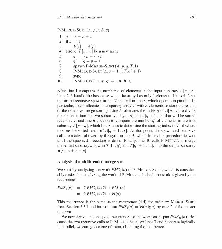
After line 1 computes the number n of elements in the input subarray AŒp : : r�,lines 2–3 handle the base case when the array has only 1 element. Lines 4–6 setup for the recursive spawn in line 7 and call in line 8, which operate in parallel. Inparticular, line 4 allocates a temporary array T with n elements to store the resultsof the recursive merge sorting. Line 5 calculates the index q of AŒp : : r� to dividethe elements into the two subarrays AŒp : : q� and AŒq C 1 : : r� that will be sortedrecursively, and line 6 goes on to compute the number q0 of elements in the firstsubarray AŒp : : q�, which line 8 uses to determine the starting index in T of whereto store the sorted result of AŒq C 1 : : r�. At that point, the spawn and recursivecall are made, followed by the sync in line 9, which forces the procedure to waituntil the spawned procedure is done. Finally, line 10 calls P-MERGE to mergethe sorted subarrays, now in T Œ1 : : q0� and T Œq0 C 1 : : n�, into the output subarrayBŒs : : s C r � p�.

Analysis of multithreaded merge sort

We start by analyzing the work PMS1.n/ of P-MERGE-SORT, which is consider-ably easier than analyzing the work of P-MERGE. Indeed, the work is given by therecurrence

PMS1.n/ D 2 PMS1.n=2/C PM1.n/

D 2 PMS1.n=2/C‚.n/ :

This recurrence is the same as the recurrence (4.4) for ordinary MERGE-SORT

from Section 2.3.1 and has solution PMS1.n/ D ‚.n lg n/ by case 2 of the mastertheorem.

We now derive and analyze a recurrence for the worst-case span PMS1.n/. Be-cause the two recursive calls to P-MERGE-SORT on lines 7 and 8 operate logicallyin parallel, we can ignore one of them, obtaining the recurrence


PMS1.n/ D PMS1.n=2/C PM1.n/

D PMS1.n=2/C‚.lg2 n/ : (27.10)

As for recurrence (27.8), the master theorem does not apply to recurrence (27.10),but Exercise 4.6-2 does. The solution is PMS1.n/ D ‚.lg3 n/, and so the span ofP-MERGE-SORT is ‚.lg3 n/.

Parallel merging gives P-MERGE-SORT a significant parallelism advantage overMERGE-SORT 0. Recall that the parallelism of MERGE-SORT 0, which calls the se-rial MERGE procedure, is only ‚.lg n/. For P-MERGE-SORT, the parallelism is

PMS1.n/=PMS1.n/ D ‚.n lg n/=‚.lg3 n/

D ‚.n= lg2 n/ ;

which is much better both in theory and in practice. A good implementation inpractice would sacrifice some parallelism by coarsening the base case in order toreduce the constants hidden by the asymptotic notation. The straightforward wayto coarsen the base case is to switch to an ordinary serial sort, perhaps quicksort,when the size of the array is sufficiently small.

Exercises

27.3-1Explain how to coarsen the base case of P-MERGE.

27.3-2Instead of finding a median element in the larger subarray, as P-MERGE does, con-sider a variant that finds a median element of all the elements in the two sortedsubarrays using the result of Exercise 9.3-8. Give pseudocode for an efficientmultithreaded merging procedure that uses this median-finding procedure. Ana-lyze your algorithm.

27.3-3Give an efficient multithreaded algorithm for partitioning an array around a pivot,as is done by the PARTITION procedure on page 171. You need not partition the ar-ray in place. Make your algorithm as parallel as possible. Analyze your algorithm.(Hint: You may need an auxiliary array and may need to make more than one passover the input elements.)

27.3-4Give a multithreaded version of RECURSIVE-FFT on page 911. Make your imple-mentation as parallel as possible. Analyze your algorithm.

Problems for Chapter 27 805

27.3-5 ?

Give a multithreaded version of RANDOMIZED-SELECT on page 216. Make yourimplementation as parallel as possible. Analyze your algorithm. (Hint: Use thepartitioning algorithm from Exercise 27.3-3.)

27.3-6 ?

Show how to multithread SELECT from Section 9.3. Make your implementation asparallel as possible. Analyze your algorithm.

Problems

27-1 Implementing parallel loops using nested parallelismConsider the following multithreaded algorithm for performing pairwise additionon n-element arrays AŒ1 : : n� and BŒ1 : : n�, storing the sums in C Œ1 : : n�:

SUM-ARRAYS.A; B; C /

1 parallel for i D 1 to A: length2 C Œi� D AŒi�C BŒi�

a. Rewrite the parallel loop in SUM-ARRAYS using nested parallelism (spawnand sync) in the manner of MAT-VEC-MAIN-LOOP. Analyze the parallelismof your implementation.

Consider the following alternative implementation of the parallel loop, whichcontains a value grain-size to be specified:

SUM-ARRAYS0.A; B; C /

1 n D A: length2 grain-size D ‹ // to be determined3 r D dn=grain-sizee4 for k D 0 to r � 1

5 spawn ADD-SUBARRAY.A; B; C; k � grain-sizeC 1;

min..k C 1/ � grain-size; n//

6 sync

ADD-SUBARRAY.A; B; C; i; j /

1 for k D i to j

2 C Œk� D AŒk�C BŒk�


b. Suppose that we set grain-size D 1. What is the parallelism of this implemen-tation?

c. Give a formula for the span of SUM-ARRAYS0 in terms of n and grain-size.Derive the best value for grain-size to maximize parallelism.

27-2 Saving temporary space in matrix multiplicationThe P-MATRIX-MULTIPLY-RECURSIVE procedure has the disadvantage that itmust allocate a temporary matrix T of size n n, which can adversely affect theconstants hidden by the ‚-notation. The P-MATRIX-MULTIPLY-RECURSIVE pro-cedure does have high parallelism, however. For example, ignoring the constantsin the ‚-notation, the parallelism for multiplying 1000 1000 matrices comes toapproximately 10003=102 D 107, since lg 1000 � 10. Most parallel computershave far fewer than 10 million processors.

a. Describe a recursive multithreaded algorithm that eliminates the need for thetemporary matrix T at the cost of increasing the span to ‚.n/. (Hint: Com-pute C D C C AB following the general strategy of P-MATRIX-MULTIPLY-RECURSIVE, but initialize C in parallel and insert a sync in a judiciously cho-sen location.)

b. Give and solve recurrences for the work and span of your implementation.

c. Analyze the parallelism of your implementation. Ignoring the constants in the‚-notation, estimate the parallelism on 1000 1000 matrices. Compare withthe parallelism of P-MATRIX-MULTIPLY-RECURSIVE.

27-3 Multithreaded matrix algorithmsa. Parallelize the LU-DECOMPOSITION procedure on page 821 by giving pseu-

docode for a multithreaded version of this algorithm. Make your implementa-tion as parallel as possible, and analyze its work, span, and parallelism.

b. Do the same for LUP-DECOMPOSITION on page 824.

c. Do the same for LUP-SOLVE on page 817.

d. Do the same for a multithreaded algorithm based on equation (28.13) for in-verting a symmetric positive-definite matrix.


27-4 Multithreading reductions and prefix computationsA ˝-reduction of an array xŒ1 : : n�, where˝ is an associative operator, is the value

y D xŒ1�˝ xŒ2�˝ � � � ˝ xŒn� :

The following procedure computes the˝-reduction of a subarray xŒi : : j � serially.

REDUCE.x; i; j /

1 y D xŒi �

2 for k D i C 1 to j

3 y D y ˝ xŒk�

4 return y

a. Use nested parallelism to implement a multithreaded algorithm P-REDUCE,which performs the same function with ‚.n/ work and ‚.lg n/ span. Analyzeyour algorithm.

A related problem is that of computing a ˝-prefix computation, sometimescalled a ˝-scan, on an array xŒ1 : : n�, where ˝ is once again an associative op-erator. The ˝-scan produces the array yŒ1 : : n� given by

yŒ1� D xŒ1� ;

yŒ2� D xŒ1�˝ xŒ2� ;

yŒ3� D xŒ1�˝ xŒ2�˝ xŒ3� ;

:::

yŒn� D xŒ1�˝ xŒ2�˝ xŒ3�˝ � � � ˝ xŒn� ;

that is, all prefixes of the array x “summed” using the ˝ operator. The followingserial procedure SCAN performs a˝-prefix computation:

SCAN.x/

1 n D x: length2 let yŒ1 : : n� be a new array3 yŒ1� D xŒ1�

4 for i D 2 to n

5 yŒi � D yŒi � 1�˝ xŒi �

6 return y

Unfortunately, multithreading SCAN is not straightforward. For example, changingthe for loop to a parallel for loop would create races, since each iteration of theloop body depends on the previous iteration. The following procedure P-SCAN-1performs the˝-prefix computation in parallel, albeit inefficiently:


P-SCAN-1.x/

1 n D x: length2 let yŒ1 : : n� be a new array3 P-SCAN-1-AUX.x; y; 1; n/

4 return y

P-SCAN-1-AUX.x; y; i; j /

1 parallel for l D i to j

2 yŒl� D P-REDUCE.x; 1; l/

b. Analyze the work, span, and parallelism of P-SCAN-1.

By using nested parallelism, we can obtain a more efficient ˝-prefix computa-tion:

P-SCAN-2.x/

1 n D x: length2 let yŒ1 : : n� be a new array3 P-SCAN-2-AUX.x; y; 1; n/

4 return y

P-SCAN-2-AUX.x; y; i; j /

1 if i == j

2 yŒi � D xŒi �

3 else k D b.i C j /=2c4 spawn P-SCAN-2-AUX.x; y; i; k/

5 P-SCAN-2-AUX.x; y; k C 1; j /

6 sync7 parallel for l D k C 1 to j

8 yŒl� D yŒk�˝ yŒl�

c. Argue that P-SCAN-2 is correct, and analyze its work, span, and parallelism.

We can improve on both P-SCAN-1 and P-SCAN-2 by performing the ˝-prefixcomputation in two distinct passes over the data. On the first pass, we gather theterms for various contiguous subarrays of x into a temporary array t , and on thesecond pass we use the terms in t to compute the final result y. The followingpseudocode implements this strategy, but certain expressions have been omitted:


P-SCAN-3.x/

1 n D x: length2 let yŒ1 : : n� and t Œ1 : : n� be new arrays3 yŒ1� D xŒ1�

4 if n > 1

5 P-SCAN-UP.x; t; 2; n/

6 P-SCAN-DOWN.xŒ1�; x; t; y; 2; n/

7 return y

P-SCAN-UP.x; t; i; j /

1 if i == j

2 return xŒi �

3 else4 k D b.i C j /=2c5 t Œk� D spawn P-SCAN-UP.x; t; i; k/

6 right D P-SCAN-UP.x; t; k C 1; j /

7 sync8 return // fill in the blank

P-SCAN-DOWN.�; x; t; y; i; j /

1 if i == j

2 yŒi � D � ˝ xŒi �

3 else4 k D b.i C j /=2c5 spawn P-SCAN-DOWN. ; x; t; y; i; k/ // fill in the blank6 P-SCAN-DOWN. ; x; t; y; k C 1; j / // fill in the blank7 sync

d. Fill in the three missing expressions in line 8 of P-SCAN-UP and lines 5 and 6of P-SCAN-DOWN. Argue that with expressions you supplied, P-SCAN-3 iscorrect. (Hint: Prove that the value � passed to P-SCAN-DOWN.�; x; t; y; i; j /

satisfies � D xŒ1�˝ xŒ2�˝ � � � ˝ xŒi � 1�.)

e. Analyze the work, span, and parallelism of P-SCAN-3.

27-5 Multithreading a simple stencil calculationComputational science is replete with algorithms that require the entries of an arrayto be filled in with values that depend on the values of certain already computedneighboring entries, along with other information that does not change over thecourse of the computation. The pattern of neighboring entries does not changeduring the computation and is called a stencil. For example, Section 15.4 presents


a stencil algorithm to compute a longest common subsequence, where the value inentry cŒi; j � depends only on the values in cŒi�1; j �, cŒi; j �1�, and cŒi�1; j �1�,as well as the elements xi and yj within the two sequences given as inputs. Theinput sequences are fixed, but the algorithm fills in the two-dimensional array c sothat it computes entry cŒi; j � after computing all three entries cŒi�1; j �, cŒi; j �1�,and cŒi � 1; j � 1�.

In this problem, we examine how to use nested parallelism to multithread asimple stencil calculation on an n n array A in which, of the values in A, thevalue placed into entry AŒi; j � depends only on values in AŒi 0; j 0�, where i 0 � i

and j 0 � j (and of course, i 0 ¤ i or j 0 ¤ j ). In other words, the value in anentry depends only on values in entries that are above it and/or to its left, alongwith static information outside of the array. Furthermore, we assume throughoutthis problem that once we have filled in the entries upon which AŒi; j � depends, wecan fill in AŒi; j � in ‚.1/ time (as in the LCS-LENGTH procedure of Section 15.4).

We can partition the n n array A into four n=2 n=2 subarrays as follows:

A D�

A11 A12

A21 A22

�: (27.11)

Observe now that we can fill in subarray A11 recursively, since it does not dependon the entries of the other three subarrays. Once A11 is complete, we can continueto fill in A12 and A21 recursively in parallel, because although they both dependon A11, they do not depend on each other. Finally, we can fill in A22 recursively.

a. Give multithreaded pseudocode that performs this simple stencil calculationusing a divide-and-conquer algorithm SIMPLE-STENCIL based on the decom-position (27.11) and the discussion above. (Don’t worry about the details of thebase case, which depends on the specific stencil.) Give and solve recurrencesfor the work and span of this algorithm in terms of n. What is the parallelism?

b. Modify your solution to part (a) to divide an n n array into nine n=3 n=3

subarrays, again recursing with as much parallelism as possible. Analyze thisalgorithm. How much more or less parallelism does this algorithm have com-pared with the algorithm from part (a)?

c. Generalize your solutions to parts (a) and (b) as follows. Choose an integerb � 2. Divide an nn array into b2 subarrays, each of size n=bn=b, recursingwith as much parallelism as possible. In terms of n and b, what are the work,span, and parallelism of your algorithm? Argue that, using this approach, theparallelism must be o.n/ for any choice of b � 2. (Hint: For this last argument,show that the exponent of n in the parallelism is strictly less than 1 for anychoice of b � 2.)

Notes for Chapter 27 811

d. Give pseudocode for a multithreaded algorithm for this simple stencil calcu-lation that achieves ‚.n= lg n/ parallelism. Argue using notions of work andspan that the problem, in fact, has ‚.n/ inherent parallelism. As it turns out,the divide-and-conquer nature of our multithreaded pseudocode does not let usachieve this maximal parallelism.

27-6 Randomized multithreaded algorithmsJust as with ordinary serial algorithms, we sometimes want to implement random-ized multithreaded algorithms. This problem explores how to adapt the variousperformance measures in order to handle the expected behavior of such algorithms.It also asks you to design and analyze a multithreaded algorithm for randomizedquicksort.

a. Explain how to modify the work law (27.2), span law (27.3), and greedy sched-uler bound (27.4) to work with expectations when TP , T1, and T1 are all ran-dom variables.

b. Consider a randomized multithreaded algorithm for which 1% of the time wehave T1 D 104 and T10;000 D 1, but for 99% of the time we have T1 DT10;000 D 109. Argue that the speedup of a randomized multithreaded algo-rithm should be defined as E ŒT1� =E ŒTP �, rather than E ŒT1=TP �.

c. Argue that the parallelism of a randomized multithreaded algorithm should bedefined as the ratio E ŒT1� =E ŒT1�.

d. Multithread the RANDOMIZED-QUICKSORT algorithm on page 179 by usingnested parallelism. (Do not parallelize RANDOMIZED-PARTITION.) Give thepseudocode for your P-RANDOMIZED-QUICKSORT algorithm.

e. Analyze your multithreaded algorithm for randomized quicksort. (Hint: Re-view the analysis of RANDOMIZED-SELECT on page 216.)

Chapter notes

Parallel computers, models for parallel computers, and algorithmic models for par-allel programming have been around in various forms for years. Prior editions ofthis book included material on sorting networks and the PRAM (Parallel Random-Access Machine) model. The data-parallel model [48, 168] is another popular al-gorithmic programming model, which features operations on vectors and matricesas primitives.


Graham [149] and Brent [56] showed that there exist schedulers achieving thebound of Theorem 27.1, and Blumofe and Leiserson [52] showed that any greedyscheduler achieves the bound. Blelloch [47] developed an algorithmic program-ming model based on work and span (which he called the “depth” of the com-putation) for data-parallel programming. Blumofe and Leiserson [53] gave a dis-tributed scheduling algorithm for dynamic multithreading based on randomized“work-stealing” and showed that it achieves the bound E ŒTP � � T1=P CO.T1/.Arora, Blumofe, and Plaxton [19] and Blelloch, Gibbons, and Matias [49] alsoprovided provably good algorithms for scheduling dynamic multithreaded compu-tations.

The multithreaded pseudocode and programming model were heavily influencedby the Cilk [51, 118] project at MIT and the Cilk++ [72] extensions to C++ dis-tributed by Cilk Arts, Inc. Many of the multithreaded algorithms in this chapterappeared in unpublished lecture notes by C. E. Leiserson and H. Prokop and havebeen implemented in Cilk or Cilk++. The multithreaded merge-sorting algorithmwas inspired by an algorithm of Akl [12].

The notion of sequential consistency is due to Lamport [223].

introduction to algorithms, 3rd ed. - mit press - massachusetts

Documents