introduction to algorithmic problem solving - gabriel...
TRANSCRIPT

Algorithms - Lecture 1 1
LECTURE 1:
Introduction to algorithmic problem solving

Algorithms - Lecture 1 2
Outline
• Problem solving
• What is an algorithm ?
• Properties an algorithm should have
• Describing Algorithms
• Types of data to use
• Basic operations

Algorithms - Lecture 1 3
Problem solvingExample:
Consider a rectangle of (integer) size axb.
We want to cover the rectangle with identical square pieces.
Choose the square size that leads to using the smallest number of pieces.
…..
a
b
c

Algorithms - Lecture 1 4
Problem solvingMathematical statement:
Let a and b be two non-zero natural numbers. Find the natural number c having the following properties:– c divides a and b (c is a common divisor of a and b)– c is greater than any other common divisor of a and b
Problem universe: natural numbers (a and b represent the input data, c represents the result)
Problem statement (relations between the input data and the result): find c, the greatest common divisor of a and b

Algorithms - Lecture 1 5
Problem solvingRemark:• Previous problem: compute the value of a function (that which
associates to a pair of natural numbers the greatest common divisor)
• Another kind of problems: decide if input data satisfies or not certain properties.
Example: verify if a natural number is a prime number or not
In both cases: want a method which after a finite number of (rather simple) operations produces the solution … such a method is an algorithm

Algorithms - Lecture 1 6
Outline
• Problem solving
• What is an algorithm ?
• Properties an algorithm should have
• Describing Algorithms
• Types of data to use
• Basic operations

Algorithms - Lecture 1 7
What is an algorithm ?
Different definitions …
Algorithm = something like a cooking recipe used to solve problems
Algorithm = a step by step problem solving method
Algorithm = a finite sequence of operations applied to some input data in order to obtain the solution of the problem

Algorithms - Lecture 1 8
What is the origin of the word ? Abū Abdallāh Mu ammad ibn Mūsā ʿ ḥ
al-Khowarizmi - Persian mathematician (790-840)
algorism algorithm
• He used 0 as a digit for the first time • He wrote the first book on algebra

Algorithms - Lecture 1 9
Examples
Algorithms in day by day life:• using a phone:
• pick up the phone• dial the number• talk ….
Algorithms in mathematics:• Euclid’s algorithm (it is considered to be the first algorithm)
• find the greatest common divisor of two numbers• Eratostene’s algorithm
• generate prime numbers in a range• Horner’s algorithm
• compute the value of a polynomial
Euclid (325 -265 b.C.)

Algorithms - Lecture 1 10
From a problem to an algorithmProblem: compute gcd(a,b) =
greatest common divisor of a and b
• Input data• a, b - natural values
• Solving method
• Divide a by b and store the remainder
• Divide b by the remainder and keep the new remainder
• Repeat the divisions until a zero remainder is obtained
• The result will be the last non-zero remainder
Algorithm:• Variables = abstract entities
corresponding to data
• dividend, divisor, remainder • Operations
1. Assign to the dividend the value of a and to the divisor the value of b
2. Compute the remainder of the division of the dividend by the divisor
3. Assign to the dividend the value of the previous divisor and to the divisor the previous value of the remainder
4. If the remainder is not zero go to step 2 otherwise output the result (the last nonzero remainder)

Algorithms - Lecture 1 11
From an algorithm to a programAlgorithm:• Variables = abstract entities
corresponding to data• dividend, divisor, remainder
• Operations
1. Assign to the dividend the value of a and to the divisor the value of b
2. Compute the remainder of the division of the dividend by the divisor
3. Assign to the dividend the value of the previous divisor and to the divisor the previous value of the remainder
4. If the remainder is not zero go to step 2 otherwise output the result (the last nonzero remainder)
Program = alg. description in a programming language:
• Variables: each variable has a corresponding storing region in the computer memory
• Operations: each operation can be decomposed in a few actions which can be executed by the computer
I/O M P
Very simplified model of a computer
Input/Output Memory Processingunit

Algorithms - Lecture 1 12
Outline
• Problem solving
• What is an algorithm ?
• Properties an algorithm should have
• Describing Algorithms
• Types of data to use
• Basic operations

Algorithms - Lecture 1 13
• Generality
• Finiteness
• Non-ambiguity
• Efficiency
Properties an algorithm should have

Algorithms - Lecture 1 14
• The algorithm applies to all instances of input data not only for particular instances
Example:
Let’s consider the problem of sorting a sequence of values in increasing order.
For instance:
(2,1,4,3,5) (1,2,3,4,5)
input data result
Generality

Algorithms - Lecture 1 15
Method:
Generality (cont’d)
2 1 4 3 5Step 1:
1 2 4 3 5
1 2 4 3 5
1 2 3 4 5
Step 2:
Step 3:
Step 4:
Description:
- compare the first two elements: if there are not in the desired order swap them- compare the second and the third element and do the same…..- continue until the last two elements were compared
The sequence has been sorted
Algorithms - Lecture 1 16
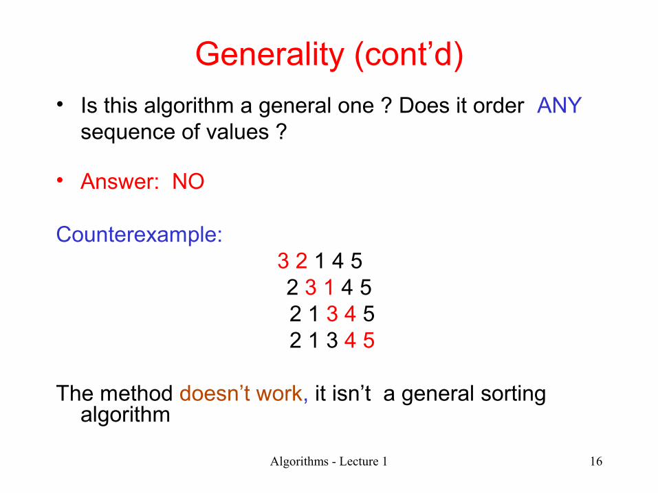
Generality (cont’d)
• Is this algorithm a general one ? Does it order ANY sequence of values ?
• Answer: NO Counterexample:
3 2 1 4 5 2 3 1 4 5 2 1 3 4 5 2 1 3 4 5
The method doesn’t work, it isn’t a general sorting algorithm

Algorithms - Lecture 1 17
Properties an algorithm should have
• Generality
• Finiteness (halting)
• Non-ambiguity
• Efficiency

Algorithms - Lecture 1 18
Finiteness
• An algorithm have to terminate, i.e. to stop after a finite number of steps
Example
Step1: Assign 1 to x;
Step2: Increase x by 2;
Step3: If x=10 then STOP;
else GO TO Step 2
How does this algorithm work ?

Algorithms - Lecture 1 19
Finiteness (cont’d)
How does this algorithm work and what does it produce?
Step1: Assign 1 to x;
Step2: Increase x by 2;
Step3: If x=10
then STOP;
else Print x; GO TO Step 2;
x=1
x=3 x=5 x=7 x=9 x=11
What can we say about this algorithm ? The algorithm generates odd numbers but it never stops !
Algorithms - Lecture 1 20
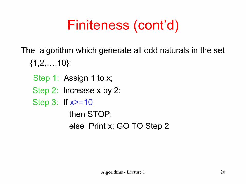
Finiteness (cont’d)
The algorithm which generate all odd naturals in the set
{1,2,…,10}: Step 1: Assign 1 to x;
Step 2: Increase x by 2;
Step 3: If x>=10
then STOP;
else Print x; GO TO Step 2

Algorithms - Lecture 1 21
What properties should an algorithm have ?
• Generality
• Finiteness
• Non-ambiguity
• Efficiency
Algorithms - Lecture 1 22
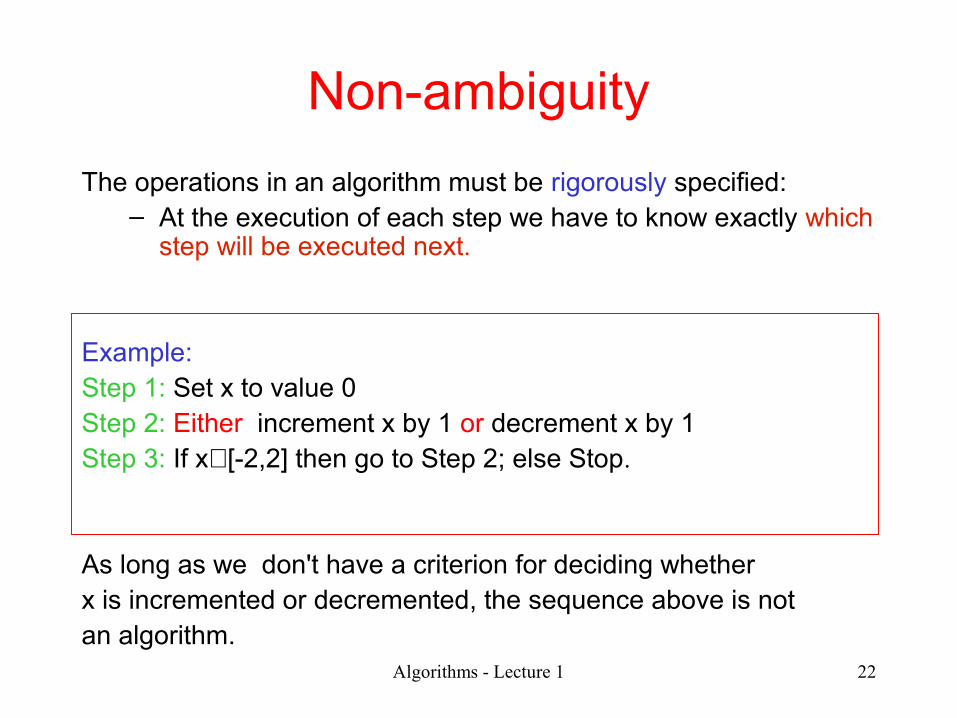
Non-ambiguity
The operations in an algorithm must be rigorously specified:– At the execution of each step we have to know exactly which
step will be executed next.
Example:Step 1: Set x to value 0Step 2: Either increment x by 1 or decrement x by 1Step 3: If x∈[-2,2] then go to Step 2; else Stop.
As long as we don't have a criterion for deciding whetherx is incremented or decremented, the sequence above is not an algorithm.

Algorithms - Lecture 1 23
Non-ambiguity (cont’d)
Modify the previous algorithm as follows:
Step 1: Set x to value 0
Step 2: Flip a coin
Step 3: coins == head
then increment x by 1
else decrement x by 1
Step 3: If x∈[-2,2] then go to Step 2, else Stop.
• This time the algorithm can be executed but … different executions may lead to different results
• This is a so called randomized algorithm

Algorithms - Lecture 1 24
Properties an algorithm should have
• Generality
• Finiteness
• Non-ambiguity
• Efficiency
Algorithms - Lecture 1 25
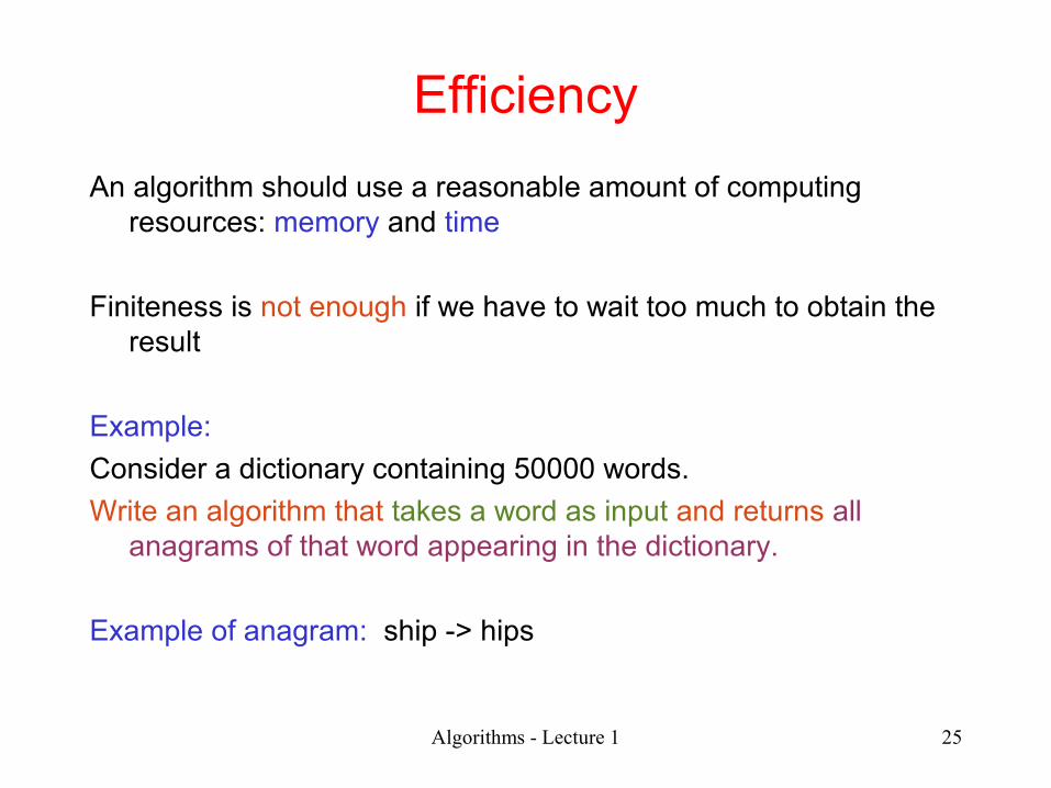
Efficiency
An algorithm should use a reasonable amount of computing resources: memory and time
Finiteness is not enough if we have to wait too much to obtain the result
Example:
Consider a dictionary containing 50000 words.
Write an algorithm that takes a word as input and returns all anagrams of that word appearing in the dictionary.
Example of anagram: ship -> hips
Algorithms - Lecture 1 26
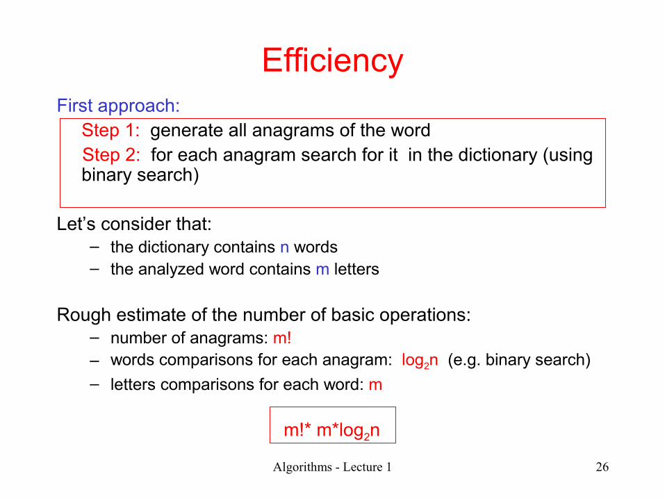
EfficiencyFirst approach:
Step 1: generate all anagrams of the word Step 2: for each anagram search for it in the dictionary (using
binary search)
Let’s consider that:– the dictionary contains n words – the analyzed word contains m letters
Rough estimate of the number of basic operations:– number of anagrams: m!– words comparisons for each anagram: log2n (e.g. binary search)
– letters comparisons for each word: m
m!* m*log2n
Algorithms - Lecture 1 27
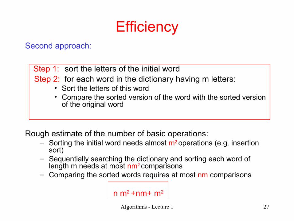
EfficiencySecond approach:
Step 1: sort the letters of the initial word Step 2: for each word in the dictionary having m letters:
• Sort the letters of this word• Compare the sorted version of the word with the sorted version
of the original word
Rough estimate of the number of basic operations:– Sorting the initial word needs almost m2 operations (e.g. insertion
sort)
– Sequentially searching the dictionary and sorting each word of length m needs at most nm2 comparisons
– Comparing the sorted words requires at most nm comparisons
n m2 +nm+ m2

Algorithms - Lecture 1 28
Efficiency
First approach Second approach
m! m log2n n m2 +n m+ m2
Example: m=12 (e.g. word algorithmics) n=50000 (number of words in dictionary) 8* 10^10 8*10^6 one basic operation (e.g.comparison)= 1ms=10-3 s24000 hours 2 hours
Thus, it is important to analyze the efficiency of the algorithm and choose more efficient elgorithms
Which approach is better ?
Algorithms - Lecture 1 29
Outline
• Problem solving
• What is an algorithm ?
• Properties an algorithm should have
• Describing Algorithms
• Types of data to use
• Basic operations

Algorithms - Lecture 1 30
How can we describe algorithms ?
Solving problems can usually be described in mathematical language
Not always adequate to describe algorithms because:
– Operations which seem elementary when described in a mathematical language are not elementary when they have to be encoded in a programming language
Example: computing a sum, computing the value of a polynomial
∑i=1
n
i=1+2+ . ..+n
Mathematical description Algorithmic description (it should be a sequence of basic operations)

Algorithms - Lecture 1 31
How can we describe algorithms ?
Two basic instruments:• Flowcharts:
– graphical description of the flow of processing steps– not used very often, somewhat old-fashioned. – however, sometimes useful to describe the overall structure of
an application• Pseudocode:
– artificial language based on• vocabulary (set of keywords)• syntax (set of rules used to construct the language’s
“phrases”)– not as restrictive as a programming language

Algorithms - Lecture 1 32
Why do we call it pseudocode ?
Because … • It is similar to a programming language (code)
• Not as rigorous as a programming language (pseudo)
In pseudocode the phrases are:
• Statements or instructions (used to describe processing steps)
• Declarations (used to specify the data)

Algorithms - Lecture 1 33
Types of dataData = container of information
Characteristics:– name
– value• constant (same value during the entire algorithm)• variable (the value varies during the algorithm)
– type• primitive (numbers, characters, truth values …)• structured (arrays)
Algorithms - Lecture 1 34
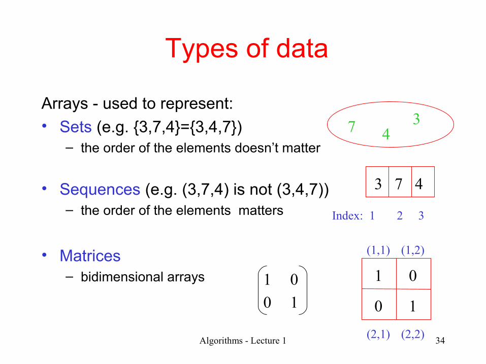
Types of data
Arrays - used to represent:• Sets (e.g. {3,7,4}={3,4,7})
– the order of the elements doesn’t matter
• Sequences (e.g. (3,7,4) is not (3,4,7))– the order of the elements matters
• Matrices – bidimensional arrays
7 34
1
0
0
1
3 7 4
Index: 1 2 3
1
10
0
(1,1) (1,2)
(2,1) (2,2)
Algorithms - Lecture 1 35
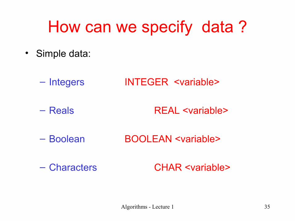
How can we specify data ?
• Simple data:
– Integers INTEGER <variable>
– Reals REAL <variable>
– Boolean BOOLEAN <variable>
– Characters CHAR <variable>

Algorithms - Lecture 1 36
How can we specify data ?
Arrays
One dimensional
<elements type> <name>[n1..n2]
(ex: REAL x[1..n])
Two-dimensional
<elements type> <name>[m1..m2, n1..n2]
(ex: INTEGER A[1..m,1..n])
Algorithms - Lecture 1 37
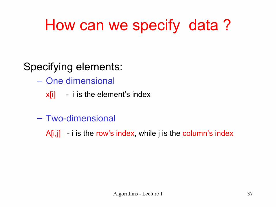
How can we specify data ?
Specifying elements:– One dimensional
x[i] - i is the element’s index
– Two-dimensional
A[i,j] - i is the row’s index, while j is the column’s index
Algorithms - Lecture 1 38
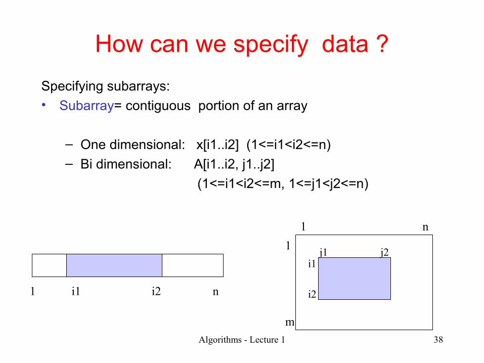
How can we specify data ?
Specifying subarrays:
• Subarray= contiguous portion of an array
– One dimensional: x[i1..i2] (1<=i1<i2<=n)
– Bi dimensional: A[i1..i2, j1..j2]
(1<=i1<i2<=m, 1<=j1<j2<=n)
1 ni2
i1
m
1
i2
1 n
j1 j2
i1

Algorithms - Lecture 1 39
Outline
• Problem solving
• What is an algorithm ?
• Properties an algorithm should have
• Describing Algorithms
• Types of data to use
• Basic instructions

Algorithms - Lecture 1 40
What are the basic instructions ?
Instruction (statement)
= action to be executed by the algorithm
There are two main types of instructions:– Simple
• Assignment (assigns a value to a variable)• Transfer (reads an input data; writes a result)• Control (specifies which is the next step to be executed)
– Structured ….

Algorithms - Lecture 1 41
• Aim: give a value to a variable• Description:
v ← <expression>
Rmk: sometimes we use := instead of ←
• Expression = syntactic construction used to describe a computation
It consists of:– Operands: variables, constant values– Operators: arithmetical, relational, logical
Assignment

Algorithms - Lecture 1 42
• Arithmetical:+ (addition), - (subtraction), *(multiplication), / (division), ^ (power), DIV (from divide) or / (integer quotient), MOD (from modulo) or % (remainder)
• Relational:= (equal), != (different), < (less than), <= (less than or equal),>(greater than) >= (greater than or equal)
• Logical: OR (disjunction), AND (conjunction), NOT (negation)
Operators

Algorithms - Lecture 1 43
Input/Output
• Aim: – read input data – output the results
• Description:
read v1,v2,… input v1, v2,…
write e1,e2,… print e1, e2,…
43
user userVariables of the algorithm
read (input)
write (print)
Input Output

Algorithms - Lecture 1 44
Instructions
Structured:– Sequence of instructions
– Conditional statement
– Loop statement

Algorithms - Lecture 1 45
condition
condition
<S1> <S2>
<S>
True False
True False
Conditional statement• Aim: allows choosing between two or several
alternatives depending on the value of a/some condition(s)
• General variant:
if <condition> then <S1> else <S2>endif
• Simplified variant:
if <condition> then <S>endif
Algorithms - Lecture 1 46
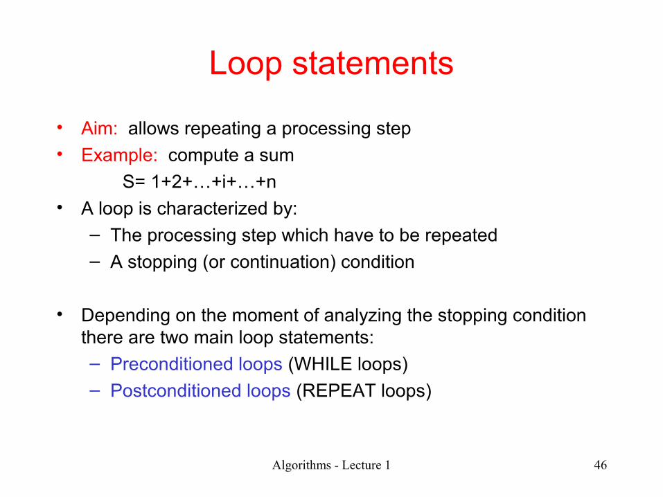
Loop statements
• Aim: allows repeating a processing step• Example: compute a sum
S= 1+2+…+i+…+n• A loop is characterized by:
– The processing step which have to be repeated– A stopping (or continuation) condition
• Depending on the moment of analyzing the stopping condition there are two main loop statements:– Preconditioned loops (WHILE loops)– Postconditioned loops (REPEAT loops)

Algorithms - Lecture 1 47
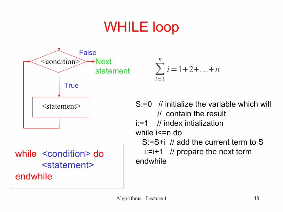
<condition>
<statement>
Nextstatement
False
True
while <condition> do <statement>endwhile
WHILE loop• First, the condition is analyzed
• If it is true then the statement is executed and the condition is analyzed again
• If the condition becomes false the control of execution passes to the next statement in the algorithm
• If the condition never becomes false then the loop is infinite
• If the condition is false from the beginning then the statement inside the loop is never executed
Algorithms - Lecture 1 48
<condition>
<statement>
Nextstatement
False
True
while <condition> do <statement>endwhile
WHILE loop
S:=0 // initialize the variable which will // contain the resulti:=1 // index intializationwhile i<=n do S:=S+i // add the current term to S i:=i+1 // prepare the next termendwhile
∑i=1
n
i=1+2+ . ..+n

Algorithms - Lecture 1 49
FOR loop
• Sometimes the number of repetitions of a processing step is known apriori
• Then we can use a counting variable which varies from an initial value to a final value using a step value
• Repetitions: v2-v1+1 if step=1
v <= v2
<statement>
Nextstatement
False
True
for v:=v1,v2,step do <statement>endfor
v:=v+step
v:=v1
v:=v1while v<=v2 do
<statement>v:=v+step
endwhile

Algorithms - Lecture 1 50
FOR loop
v <= v2
<statement>
Nextstatement
False
True
for v:=v1,v2,step do <statement>endfor
v:=v+step
v:=v1
S:=0 // initialize the variable which will // contain the result
for i:=1,n do S:=S+i // add the term to Sendfor
∑i=1
n
i=1+2+ . ..+n
Algorithms - Lecture 1 51
REPEAT loop
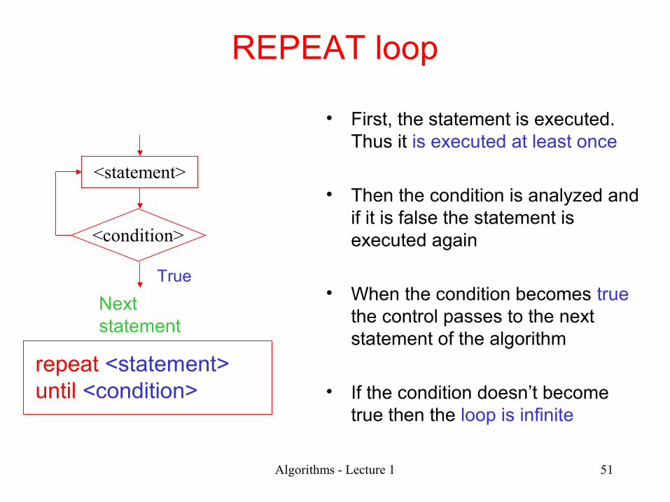
• First, the statement is executed. Thus it is executed at least once
• Then the condition is analyzed and if it is false the statement is executed again
• When the condition becomes true the control passes to the next statement of the algorithm
• If the condition doesn’t become true then the loop is infinite
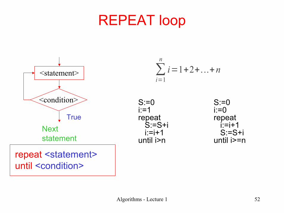
<condition>
<statement>
Nextstatement
True
repeat <statement>until <condition>
Algorithms - Lecture 1 52
REPEAT loop
<condition>
<statement>
Nextstatement
True
repeat <statement>until <condition>
S:=0 i:=1repeat S:=S+i i:=i+1until i>n
∑i=1
n
i=1+2+ . ..+n
S:=0 i:=0repeat i:=i+1 S:=S+iuntil i>=n

Algorithms - Lecture 1 53
REPEAT loop
Any REPEAT loop can be transformed in a WHILE loop:
<statement>
while NOT <condition> DO
<statement>
endwhile
<condition>
<statement>
Nextstatement
True
repeat <statement>until <condition>

Algorithms - Lecture 1 54
Summary
• Algorithms are step-by-step procedures for problem solving
• They should have the following properties:•Generality•Finiteness•Non-ambiguity (rigorousness)•Efficiency
• Data processed by an algorithm can be • simple• structured (e.g. arrays)
•We describe algorithms by means of pseudocode
Algorithms - Lecture 1 55
Summary
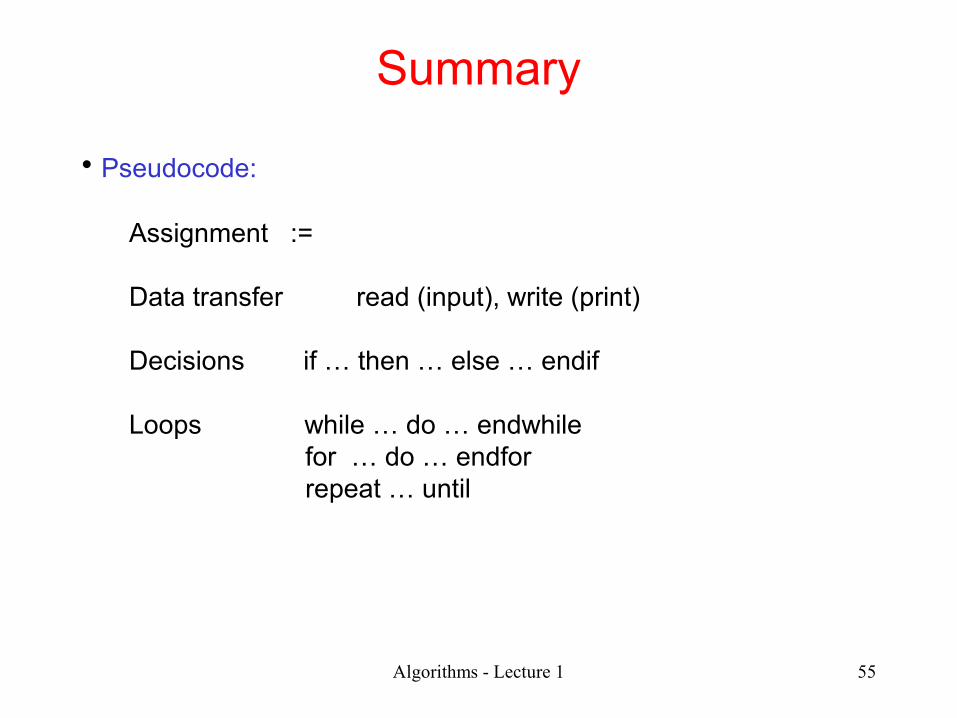
• Pseudocode:
Assignment :=
Data transfer read (input), write (print)
Decisions if … then … else … endif
Loops while … do … endwhile for … do … endfor repeat … until

Algorithms - Lecture 1 56
Next lecture …
• Other examples of algorithms
• Subalgorithms
• A word on correctness