introduction - st. john's university

HOCHSCHILD HOMOLOGY RELATIVE TO A FAMILY OF GROUPS

ANDREW NICAS∗ AND DAVID ROSENTHAL

Abstract. We define the Hochschild homology groups of a group ring ZG relative to afamily of subgroups F of G. These groups are the homology groups of a space which canbe described as a homotopy colimit, or as a configuration space, or, in the case F is thefamily of finite subgroups of G, as a space constructed from stratum preserving paths.An explicit calculation is made in the case G is the infinite dihedral group.

Introduction

The Hochschild homology of an associative, unital ring A with coefficients in an A-A

bimodule M is defined via homological algebra by HH∗(A,M) := TorA⊗Aop

∗ (M,A) where

Aop is the opposite ring of A. In the case A = ZG, the integral group ring of a discrete

group G, and M = ZG, the Hochschild homology groups HH∗(ZG) := HH∗(ZG,ZG)

have the following homotopy theoretic description. The cyclic bar construction associates

to a group G a simplicial set N cyc(G) whose homology is HH∗(ZG). Viewing G as a

category, G, consisting of a single object and with morphisms identified with the elements

of G, consider the functor N from G to the category of sets given by N(∗) = G and, for a

morphism g ∈ G = MorG(∗, ∗), the map N(g) : G→ G is conjugation, sending x to g−1xg.

The geometric realization of N cyc(G) is homotopy equivalent to hocolimN , the homotopy

colimit of N . There is also a natural homotopy equivalence |N cyc(G)| → L(BG) (see [12,

Theorem 7.3.11]) where BG is the classifying space of G and L(BG) is the free loop space

of BG, i.e., the space of continuous maps of the circle into BG. In particular, there are

isomorphisms:

HH∗(ZG) ∼= H∗(hocolimN) ∼= H∗(L(BG)).

A family of subgroups of a group G is a non-empty collection of subgroups of G that is

closed under conjugation and finite intersections. In this paper we define the Hochschild

Date: January 31, 2008.2000 Mathematics Subject Classification. 16E40, 19D55, 55R35.Key words and phrases. Hochschild homology, family of subgroups, classifying space.∗Partially supported by a grant from the Natural Sciences and Engineering Research Council of Canada.

1

2 NICAS AND ROSENTHAL

homology of a group ring ZG relative to a family of subgroups F of G, denoted HHF∗ (ZG).

This is accomplished at the level of spaces. We define a functor NF : Or(G,F) → CGH

where Or(G,F) is the orbit category of G with respect to F and CGH is the category

of compactly generated Hausdorff spaces. By definition, HHF∗ (ZG) := H∗(hocolimNF).

If F is the trivial family, i.e., contains only the trivial group, then N ∼= NF and so

HHF∗ (ZG) = HH∗(ZG).

For a discrete group G and any family F , let EFG be a universal space for G-actions

with isotropy in F . That is, EFG is a G-CW complex whose isotropy groups belong to

F and for every H in F , the fixed point set (EFG)H is contractible. Given a G-space X,

let F (X) be the configuration space of pairs of points in X which lie on the same G-orbit.

This space inherits a G-action via restriction of the diagonal action of G on X ×X.

Suppose that G is countable and that the family F of subgroups is also countable.

Theorem A. There is a natural homotopy equivalence hocolimNF ' G\F (EFG) .

Indeed, this homotopy equivalence is a homeomorphism for an appropriate model of the

homotopy colimit (see Theorem 3.7 and Corollary 3.8).

Specializing to the case where F is the family of finite subgroups of G, we write

EG := EFG and BG := G\EG. Let Pmsp(BG) denote the space of marked stratum preserving

paths in BG consisting of stratum preserving paths in BG (with the orbit type partition)

whose endpoints are “marked” by an orbit of the diagonal action of G on EG × EG. We

show (see Theorem 4.26(i)):

Theorem B. There is a natural homotopy equivalence hocolimNF ' Pmsp(BG).

Theorem B is a consequence of Theorem A and a homotopy equivalence G\F (X) 'Pm

sp(G\X) which is valid for any proper G-CW complex X (see Theorem 4.20). The

Covering Homotopy Theorem of Palais (Theorem 4.7) plays a key role in the proof of the

latter result.

If EG satisfies a certain isovariant homotopy theoretic condition then Pmsp(BG) is ho-

motopy equivalent to a subspace Lmsp(BG) ⊂ Pm

sp(BG) which we call the marked stratified

free loop space of BG (see Theorem 4.26(ii)). We show that this condition is satisfied for

appropriate models of EG in the cases:

(1) G is torsion free (see Remark 4.25); note that in this case EG = EG, a universal

space for free proper G-actions,

HOCHSCHILD HOMOLOGY 3

(2) G belongs to a particular class of groups which includes the infinite dihedral group

and hyperbolic or euclidean triangle groups (see Examples 5.5 and 5.6),

(3) finite products of such groups (see Remark 5.7).

In the case G is torsion free, Lmsp(BG) is homeomorphic to L(BG) by Proposition

4.22 and so our result can be viewed as a generalization of the homotopy equivalence

|N cyc(G)| ' L(BG).

There is an equivariant map EG→ EG which is unique up to equivariant homotopy. This

map induces a map G\F (EG)→ G\F (EG), equivalently, a map hocolimN → hocolimNF ,

where F is the family of finite subgroups of G. We explicitly compute this map in the case

where G = D∞, the infinite dihedral group. In particular, this yields a computation of the

homomorphism HH∗(ZD∞) → HHF∗ (ZD∞); see Section 6.

The paper is organized as follows. In Section 1 we review some aspects of the theory

of homotopy colimits. The functor NF : Or(G,F) → CGH is defined in Section 2 thus

yielding the space N(G,F) := hocolimNF which we call the Hochschild complex of G with

respect to the family of subgroups F . In Section 3 we study the configuration space F (X)

in a general context and give an alternative description of N(G,F) as the orbit space

G\F (EFG). The homotopy equivalence G\F (X) ' Pmsp(G\X), for any proper G-CW

complex X, is established in Section 4. We also show in this section that if EG satisfies a

certain isovariant homotopy theoretic condition then Pmsp(BG) is homotopy equivalent to

the subspace Lmsp(BG) ⊂ Pm

sp(BG). In Section 5, we show that this condition is satisfied

for a class of groups which includes the infinite dihedral group and hyperbolic or euclidean

triangle groups. In Section 6 we analyze the map G\F (EG) → G\F (EG), and compute

it explicitly in the case G = D∞ thereby obtaining a computation of the homomorphism

HH∗(ZD∞) → HHF∗ (ZD∞).

1. Homotopy Colimits and Spaces Over a Category

In this section we provide some categorical preliminaries, following Davis and Luck [7],

that will be used in Section 2 to define a Hochschild complex associated to a family of

subgroups. Throughout Sections 1 and 2 we work in the category of compactly generated

Hausdorff spaces, denoted by CGH. 1

1Given a Hausdorff space Y , the associated compactly generated space, kY , is the space with the sameunderlying set and with the topology defined as follows: a closed set of kY is a set that meets each compactset of Y in a closed set. Y is an object of CGH if and only if Y = kY , i.e., Y is compactly generated. The


Let C be a small category. A covariant (contravariant) C-space, is a covariant (con-

travariant) functor from C to CGH. If X is a contravariant C-space and Y is a covariant

C-space, then their tensor product is defined by

X ⊗C Y =∐

C∈obj(C)

X(C)× Y (C) / ∼

where ∼ is the equivalence relation generated by

(X(φ)(x), y

)∼(x, Y (φ)(y)

)for all φ ∈ MorC(C,D), x ∈ X(D) and y ∈ Y (C).

A map of C-spaces is a natural transformation of functors. Given a C-space X and a

topological space Z, let X ×Z be the C-space defined by (X ×Z)(C) = X(C)×Z, where

C is an object in C. Two maps of C-spaces, α, β : X → X ′, are C-homotopic if there is a

natural transformation H : X × [0, 1] → X ′ such that H|X×{0} = α and H|X×{1} = β. A

map α : X → X ′ is a C-homotopy equivalence if there is a map of C-spaces β : X ′ → X such

that αβ is C-homotopic to idX′ and βα is C-homotopic to idX . The map α : X → X ′ is a

weak C-homotopy equivalence if for every object C in C, the map α(C) : X(C) → X ′(C)

is an ordinary weak homotopy equivalence. Two C-spaces X and X ′ are C-homeomorphic

if there are maps α : X → X ′ and α′ : X ′ → X such that α′α = idX and αα′ = idX′ . If

X and X ′ are C-homeomorphic contravariant C-spaces and Y and Y ′ are C-homeomorphic

covariant C-spaces, then X ⊗C Y is homeomorphic to X ′ ⊗C Y ′.A contravariant free C-CW complex X is a contravariant C-space X together with a

filtration

∅ = X−1 ⊂ X0 ⊂ X1 ⊂ · · · ⊂ Xn ⊂ · · · ⊂ X =⋃n≥0

Xn

such that X = colimn→∞Xn and for any n ≥ 0, the n-skeleton, Xn, is obtained from

the (n − 1)-skeleton Xn−1 by attaching free contravariant C − n-cells. That is, there is a

product of two spaces Y , Z in CGH is defined by Y × Z := k(Y × Z) where Y × Z on the right side hasthe product topology. Function space topologies in CGH are defined by applying k to the compact-opentopology. In Sections 3 and 4 we work in the category TOP of all topological spaces and we will haveoccasion to compare the topologies on Y and kY (see Proposition 3.6).


pushout of C-spaces of the form∐i∈In MorC(−, Ci)× Sn−1

� _

��

// Xn−1� _

��∐i∈In MorC(−, Ci)×Dn // Xn

where In is an indexing set and Ci is an object in C. A covariant free C-CW complex

is defined analogously, the only differences being that the C-space is covariant and the

C-space MorC(Ci,−) is used in the pushout diagram instead of MorC(−, Ci).A free C-CW complex should be thought of as a generalization of a free G-CW complex.

The two notions coincide if C is the category associated to the group G, i.e., the category

with one object and one morphism for every element of G.

Let EC be a contravariant free C-CW complex such that EC(C) is contractible for every

object C of C. Such a C-space always exists and is unique up to homotopy type [7, Section

3]. One particular example is defined as follows.

Let BbarC be the bar construction of the classifying space of C, i.e., BbarC = |N.C|, the

geometric realization of the nerve of C. Let C be an object in C. The undercategory, C ↓ C,is the category whose objects are pairs (f,D), where f : C → D is a morphism in C, and

whose morphisms, p : (f,D)→ (f ′, D′), consist of a morphism p : D → D′ in C such that

p ◦ f = f ′. Notice that a morphism φ : C → C ′ induces a functor φ∗ : (C ′ ↓ C)→ (C ↓ C)defined by φ∗(f,D) = (f ◦ φ,D). Let EbarC : C → CGH be the contravariant functor

defined by

EbarC(C) = Bbar(C ↓ C)

EbarC(φ : C → C ′) = Bbar(φ∗)

This is a model for EC. Furthermore, EbarC ⊗C ∗ is homeomorphic to BbarC [7, Section 3].

Lemma 1.1. [7, Lemma 1.9] Let F : D → C be a covariant functor, Z a covariant D-space

and X a contravariant C-space. Let F∗Z be the covariant C-space MorC(F (−D),−C)⊗D Z,

where −C denotes the variable in C and −D denotes the variable in D. Then

X ⊗C F∗Z → (X ◦ F )⊗D Z

is a homeomorphism.


Proof. The map e : X ⊗C(MorC(F (−D),−C)⊗D Z

)−→(X ◦ F )⊗D Z is defined by

e([x, [f, y]

])= [X(f)(x), y],

where x ∈ X(C), y ∈ Z(D) and f ∈ MorC(F (D), C), for objects C in C and D in D. The

inverse is given by mapping [w, z] ∈ (X ◦F )⊗DZ to[w, [idF (D), z]

], where w ∈ (X ◦F )(D)

and z ∈ Z(D). �

Definition 1.2. Let Y be a covariant C-space. Then

hocolimC

Y := EbarC ⊗C Y.

A map, α : Y → Y ′, of C-spaces induces a map α∗ : hocolimC Y → hocolimC Y′. If ∗ is

the C-space that sends every object to a point, then

hocolimC

∗ = EbarC ⊗C ∗ ∼= BbarC.

Therefore, the collapse map, Y → ∗, induces a map π : hocolimC Y → BbarC.There are several well known constructions for the homotopy colimit, each yielding the

same space up to homotopy equivalence (see Talbert [22, Theorem 1.2]). In particular,

using the transport category, TC(Y ), one can define the homotopy colimit of Y to be

BbarTC(Y ). Recall that an object of TC(Y ) is a pair (C, x), where C is an object of C and

x ∈ Y (C), and a morphism φ : (C, x)→ (C ′, x′) is a morphism φ : C → C ′ in C such that

Y (φ)(x) = x′. The following lemma shows that BbarTC(Y ) is not only homotopy equivalent

to our definition of the homotopy colimit of Y , but is in fact homeomorphic to hocolimC Y .

Lemma 1.3. Let Y be a covariant C-space. Then EbarTC(Y )⊗TC(Y ) ∗ is homeomorphic to

EbarC ⊗C Y .

Proof. By Lemma 1.1, there is a homeomorphism

EbarC ⊗C π∗(∗)→ (EbarC ◦ π)⊗TC(Y ) ∗

where π : TC(Y ) → C is the projection functor which sends an object (C, x) to C. We

will show that EbarC ⊗C π∗(∗) is homeomorphic to EbarC ⊗C Y and (EbarC ◦ π) ⊗TC(Y ) ∗ is

homeomorphic to EbarTC(Y )⊗TC(Y ) ∗.Let C be an object of C. A point in π∗(∗)(C) = MorC(π(−), C) ⊗TC(Y ) ∗ is represented

by a morphism ψ : π(D, x)→ C in C, where (D, x) is an object of TC(Y ). Define a natural

transformation β : π∗(∗) → Y by β(C)([ψ]) = Y (ψ)(x). The inverse, β−1 : Y → π∗(∗), is


defined by β−1(C)(y) = [idC ], where y ∈ Y (C) and idC : π(C, y)→ C is the identity. This

induces a homeomorphism EbarC ⊗C π∗(∗)→ EbarC ⊗C Y .

Now let (C, x) be an object of TC(Y ). Then (EbarC ◦π)(C, x) = EbarC(C) = Bbar(C ↓ C),and EbarTC(Y )(C, x) = Bbar((C, x) ↓ TC(Y )). For each (C, x), there is an isomorphism of

categories F(C,x) : C ↓ C → (C, x) ↓ TC(Y ) given by F(C,x)(f, A) =(f, (A, Y (f)(x))

), where

f : C → A in C. If φ : (f, A) → (f ′, A′) is a morphism in C ↓ C, then F(C,x)(φ) = φ :(f, (A, Y (f)(x))

)→(f ′, (A′, Y (f ′)(x))

)is a morphism in (C, x) ↓ TC(Y ) since f ′ = φ ◦ f .

The inverse of F is the obvious one. Define the natural transformation α : EbarC ◦ π →EbarTC(Y ) by α(C, x) = Bbar(F(C,x)) : Bbar(C ↓ C) → Bbar((C, x) ↓ TC(Y )), and its inverse

by α−1(C, x) = Bbar(F−1(C,x)). This induces a homeomorphism (EbarC ◦ π) ⊗TC(Y ) ∗ →

EbarTC(Y )⊗TC(Y ) ∗. �

If H : D → C is a covariant functor and Y is a covariant C-space, then there is a

functor H : TD(Y ◦ H) → TC(Y ) given by H(D, x) = (H(D), x). This induces a map

Bbar(H) : BbarTD(Y ◦H) → BbarTC(Y ). The functor H also induces a map H : EbarD ⊗DY ◦ H → EbarC ⊗C Y given by H([x, y]) = [Bbar(HD)(x), y], where x ∈ Bbar(D ↓ D),

y ∈ Y (H(D)) and HD : (D ↓ D)→ (H(D) ↓ C) is the obvious functor induced by H. The

maps Bbar(H) and H are equivalent via the homeomorphism from Lemma 1.3. It is also

straightforward to check that the composition of the homeomorphism from Lemma 1.3

with Bbar(π) : BbarTC(Y )→ BbarC is equal to π : hocolimC Y → BbarC.The transport category definition of the homotopy colimit is employed to prove the

following useful lemma.

Lemma 1.4. Let H : D → C be a covariant functor and Y be a covariant C-space. Then

(1) hocolimD Y ◦Hπ

��

H // hocolimC Y

π��

BbarDBbar(H)

// BbarCis a pullback diagram.

Proof. Form the pullback diagram

P(H, π)

��

// TC(Y )

π

��D H // C


in the category of small categories. The category P(H, π) is a subcategory of TC(Y )×D,

where an object ((C, x), D) satisfies H(D) = C, and a morphism (α, β) : ((C, x), D) →((C ′, x′), D′) satisfies α = H(β). If ((C, x), D) is an object of P(H, π), then (C, x) is an

object of TD(Y ◦H), and if (α, β) : ((C, x), D)→ ((C ′, x′), D′) is a morphism of P(H, π),

then β : (D, x)→ (D′, x′) is a morphism of TD(Y ◦H) since (Y ◦H)(β)(x) = F (α)(x) = x′.

Hence, we have a functor from P(H, π) to the transport category TD(Y ◦H) with inverse

given by (D, x) 7→ (H(D), x), D) and β : (D, x)→ (D′, x′) 7→ (H(β), β) : (H(D), x), D)→(H(D′), x′), D′). Therefore, we have the pullback diagram

TD(Y ◦H)

π

��

H // TC(Y )

π

��D H // C

Applying Bbar produces the pullback diagram

Bbar(TD(Y ◦H))

��

// Bbar(TC(Y ))

��BbarD // BbarC

The result now follows from two applications of Lemma 1.3. �

2. The Orbit Category and the Hochschild Complex

Let G be a discrete group and F a family of subgroups of G that is closed under

conjugation and finite intersections. Let O = Or(G,F) denote the orbit category of G with

respect to F . The objects of O are the homogeneous spaces G/H, with H ∈ F , considered

as left G-sets. Morphisms are all G-equivariant maps. Therefore, MorO(G/H,G/K) =

{rg | g−1Hg ≤ K}, where rg is right multiplication by g, i.e., rg(uH) = (ug)H for uH ∈G/H. If F is the family of all subgroups of G, then O is called the orbit category. If F is

taken to be the trivial family, then O is the usual category associated to the group G.

Definition 2.1 (Hochschild complex of a group associated to a family of subgroups).

Let O × O be the category whose objects are ordered pairs of objects in O and whose

morphisms are ordered pairs of morphisms in O. Let Ad : O×O → CGH be the covariant

functor defined byAd(G/H1, G/H2) = H1\G/H2

Ad(rg1 , rg2)(H1uH2) = K1g1−1ug2K2,


where H1\G/H2 is the set of (H1, H2) double cosets in G with the discrete topology and

(rg1 , rg2) : (G/H1, G/H2)→ (G/K1, G/K2) is a morphism in O×O, and let NF = Ad◦∆,

where ∆ : O → O ×O is the diagonal functor. Define

N(G,F) = hocolimO

NF .

We call N(G,F) the Hochschild complex of G associated to the family F .

Remark 2.2. More generally, NF can be defined in the case G is a locally compact topo-

logical group and the members of the family of subgroups F are closed subgroups of G by

giving H1\G/H2 the quotient topology.

If F is the trivial family, {1}, then N(G, {1}) is homotopy equivalent to |N cyc(G)|,the geometric realization of the cyclic bar construction ([12, 7.3.10]); indeed, using the

2-sided bar construction as a model for the homotopy colimit of N{1} yields a complex

homeomorphic to |N cyc(G)|. We refer to N(G, {1}) as the classical Hochschild complex of

G.

Definition 2.3. The Hochschild homology of a group ring ZG relative to a family of

subgroups F of G is defined to be

HHF∗ (ZG) := H∗(N(G,F); Z).

Using diagram (1) with Ad and NF , we obtain the following pullback diagram

(2) N(G,F)

��

// hocolimO×O Ad

π��

BbarOBbar(∆)

// Bbar(O ×O)

Lemma 2.4. Let ∆ : O → O ×O denote the diagonal functor. Then hocolimO×O Ad is

homeomorphic to (Ebar(O ×O) ◦∆)⊗O ∗.

Proof. Let T : O ×O → CGH denote the covariant functor

MorO×O(∆(−O),−O×O)⊗O ∗.

Note that MorO(G/L,G/M) = {rg | g−1Lg ≤ M} ∼= {gM | g−1Lg ≤ M}. Using this

identification, let α : Ad→ T be the natural transformation defined by

α(H\G/K)(HgK) = [r1, rg],


where (r1, rg) ∈ MorO×O((G/1, G/1), (G/H,G/K)). The inverse of α is given by

α−1(G/H,G/K)([rg1 , rg2 ]) = Hg−11 g2K,

where (rg1 , rg2) ∈ MorO×O((G/L,G/L), (G/H,G/K)) and G/L is an object in O. Thus,

Ad is naturally equivalent to T . Therefore,

Ebar(O ×O)⊗O×O Adα∗∼=

// Ebar(O ×O)⊗O×O Te

∼=// (Ebar(O ×O) ◦∆)⊗O ∗,

where e is the homeomorphism from Lemma 1.1. �

Definition 2.5. Let G be a discrete group and F be a family of subgroups of G. A

universal space for G-actions with isotropy in F is a G-CW complex, EFG, whose isotropy

groups belong to F and for every H in F , the fixed point set (EFG)H is contractible. Such

a space is unique up to G-equivariant homotopy equivalence [14].

Davis and Luck [7, Lemma 7.6] showed that given any model for EO, EO ⊗O ∇ is a

universal G-space with isotropy in F , where ∇ : O → CGH is the covariant functor that

sends G/H to itself and rg : G/H → G/K to itself.

Theorem 2.6. Let G be a discrete group and F a family of subgroups of G. Then

N(G,F)

��

// G\(EFG× EFG)

ρ×ρ��

G\EFG∆ // G\EFG×G\EFG

is a pullback diagram, where EFG = EbarO ⊗O ∇, ρ : EFG → G\EFG is the orbit map,

ρ× ρ is the map induced by ρ× ρ, and ∆ is the diagonal map.

Proof. There is a homeomorphism,

f : (Ebar(O ×O) ◦∆)⊗O ∗ → G\(EFG× EFG),

defined by f([(x, y)]) = q([x, eK], [y, eK]), where

(x, y) ∈ Bbar(G/K ↓ O)× Bbar(G/K ↓ O) ∼= (Ebar(O ×O) ◦∆)(G/K)

and q : EFG × EFG → G\(EFG × EFG) is the orbit map. The inverse of f is given

by f−1(q([x, g1K], [y, g2K])) = [Bbar(ε∗g1K)(x),Bbar(ε∗g2K)(y)], where εgiK : G/1 → G/K


is right multiplication by gi. Here we have identified Bbar(C × D) with BbarC × BbarD.

Similarly, there is a homeomorphism

f : BbarO ∼= EbarO ⊗O ∗ → G\EFG,

defined by f([x]) = ρ([x, eK]), where x ∈ Bbar(G/K ↓ O) and ρ : EFG → G\EFG is the

orbit map. The inverse of f is given by (f)−1(ρ([x, gK])) = [Bbar(ε∗gK)(x)].

Using the homeomorphism from Lemma 2.4, we get the commutative diagram

hocolimO×O Ad

��

∼=e◦α∗ // (Ebar(O ×O) ◦∆)⊗O ∗ ∼=

f // G\(EFG× EFG)

ρ×ρ��

Bbar(O ×O)∼= // BbarO × BbarO

f×f

∼= // G\EFG×G\EFG

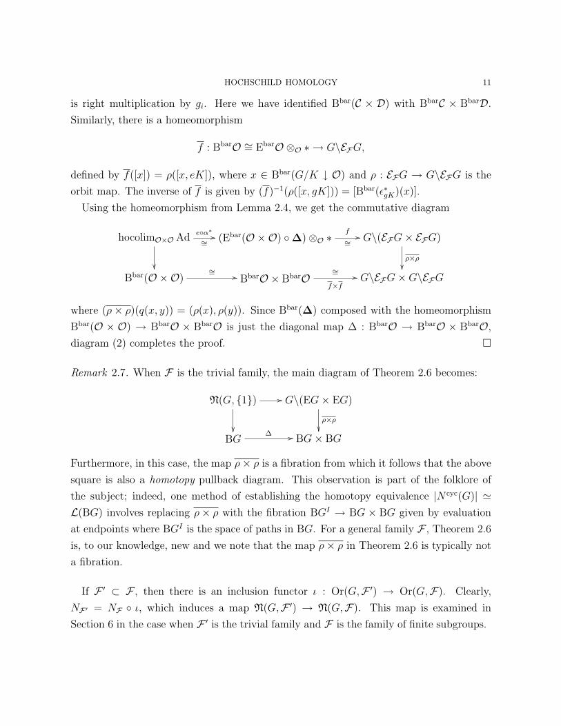
where (ρ× ρ)(q(x, y)) = (ρ(x), ρ(y)). Since Bbar(∆) composed with the homeomorphism

Bbar(O × O) → BbarO × BbarO is just the diagonal map ∆ : BbarO → BbarO × BbarO,

diagram (2) completes the proof. �

Remark 2.7. When F is the trivial family, the main diagram of Theorem 2.6 becomes:

N(G, {1})

��

// G\(EG× EG)

ρ×ρ��

BG∆ // BG× BG

Furthermore, in this case, the map ρ× ρ is a fibration from which it follows that the above

square is also a homotopy pullback diagram. This observation is part of the folklore of

the subject; indeed, one method of establishing the homotopy equivalence |N cyc(G)| 'L(BG) involves replacing ρ× ρ with the fibration BGI → BG × BG given by evaluation

at endpoints where BGI is the space of paths in BG. For a general family F , Theorem 2.6

is, to our knowledge, new and we note that the map ρ× ρ in Theorem 2.6 is typically not

a fibration.

If F ′ ⊂ F , then there is an inclusion functor ι : Or(G,F ′) → Or(G,F). Clearly,

NF ′ = NF ◦ ι, which induces a map N(G,F ′) → N(G,F). This map is examined in

Section 6 in the case when F ′ is the trivial family and F is the family of finite subgroups.


3. The Configuration Space F (X)

In this section we investigate, in a general context, some basic properties of the config-

uration space, F (X), of pairs of points in a G-space X which lie on the same G-orbit.

Let G be a topological group. The category of left G-spaces, denoted by G TOP, is

the category whose objects are left G-spaces, i.e., topological spaces X together with a

continuous left G-action G ×X → X, written as (g, x) 7→ gx, and whose morphisms are

continuous equivariant maps f : X → Y . Henceforth, we abbreviate “left G-space” to

“G-space”.

Given aG-spaceX, define AX : G×X →X×X by AX(g, x) := (x, gx) for (g, x) ∈ G×X.

Note that AX is continuous and G-equivariant where G×X is given the left G action

(3) h(g, x) := (hgh−1, hx) for h, g ∈ G and x ∈ X

and X×X is given the diagonal G-action. Hence the image of AX is a G-invariant subspace

of X ×X.

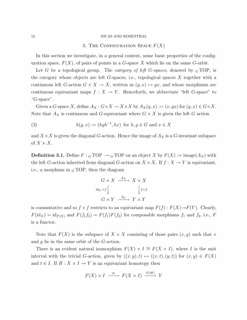
Definition 3.1. Define F : G TOP → G TOP on an object X by F (X) := image(AX) with

the left G-action inherited from diagonal G-action on X×X. If f : X → Y is equivariant,

i.e., a morphism in G TOP, then the diagram

G×X AX−−−→ X ×X

idG×fy yf×f

G× Y AY−−−→ Y × Yis commutative and so f ×f restricts to an equivariant map F (f) : F (X)→F (Y ). Clearly,

F (idX) = idF (X) and F (f1f2) = F (f1)F (f2) for composable morphisms f1 and f2, i.e., F

is a functor.

Note that F (X) is the subspace of X × X consisting of those pairs (x, y) such that x

and y lie in the same orbit of the G-action.

There is an evident natural isomorphism F (X) × I ∼= F (X × I), where I is the unit

interval with the trivial G-action, given by ((x, y), t) 7→ ((x, t), (y, t)) for (x, y) ∈ F (X)

and t ∈ I. If H : X × I → Y is an equivariant homotopy then

F (X)× I∼=−−−→ F (X × I)

F (H)−−−→ Y


is an equivariant homotopy from F (H0) to F (H1), where Ht := H(−, t). Hence F factors

through the homotopy category of G TOP with the following consequence.

Proposition 3.2. If the map f : X → Y is an equivariant homotopy equivalence then

F (f) : F (X) → F (Y ) is an equivariant homotopy equivalence. �

Definition 3.3. In the category TOP of all topological spaces we use the following notation

for the standard pullback construction. Given maps e : A → Z and f : B → Z define

E(e, f) := {(x, y) ∈ A × B | e(x) = f(y)} topologized as a subspace of A × B with the

product topology. The maps p1 : E(e, f)→ A and p2 : E(e, f)→ B are given, respectively,

by the restriction of the projections A×B → A and A×B → B. The square

E(e, f)p2−−−→ B

p1

y yfA

e−−−→ Z

is a pullback diagram in TOP which we refer to as a standard pullback diagram.

Proposition 3.4. There is a pullback diagram

F (X)i−−−→ X × X

q

y yρ×ρG\X ∆−−−→ G\X ×G\X

where i is the inclusion F (X) = image(AX) ⊂ X ×X, ρ : X → G\X is the orbit map, ∆

is the diagonal map and q : F (X) → G\X is given by q((x, y)) = ρ(y) for (x, y) ∈ F (X).

Proof. The standard pullback construction yields

E(∆, ρ× ρ) = {(ρ(x), x1, x2) ∈ (G\X)×X ×X | ρ(x) = ρ(x1) = ρ(x2)}.

The map j : F (X) → E(∆, ρ × ρ) given by j((x, y)) = (ρ(x), x, y) is a homeomorphism

with inverse (ρ(x), x, y) 7→ (x, y). Also p1j = q and p2j = i where p1 : E(∆, ρ×ρ)→ G\Xand p2 : E(∆, ρ× ρ) → X ×X are the restrictions of the corresponding projections. �

The space G\F (X) can also be described as a pullback as follows:


Theorem 3.5. There is a pullback diagram

G\F (X)ı−−−→ G\(X ×X)

q


where ı, q and ρ× ρ are induced by i, q and ρ× ρ respectively (as in Proposition 3.4).

Proof. The pullback diagram of Proposition 3.4 factors as:

F (X)i−−−→ X ×X

q′

y yρ′E(∆, ρ× ρ)

p2−−−→ G\(X ×X)

p1


where ρ′ : X ×X → G\(X ×X) is the orbit map, q′((x, y)) = (ρ(x), ρ′(x, y)) for (x, y) ∈F (X) and E(∆, ρ× ρ) together with the maps p1, p2 is the standard pullback construction.

The outer square in the above diagram is a pullback by Proposition 3.4 and the lower square

is a pullback by construction. It follows that the upper square is a pullback. By Lemma

3.18, q′ induces a homeomorphism G\F (X) ∼= E(∆, ρ× ρ). �

A Hausdorff space X is compactly generated if a set A ⊂ X is closed if and only if it

meets each compact set of X in a closed set.

Proposition 3.6. Suppose that G is a countable discrete group and that X is a count-

able G-CW complex i.e., X has countably many G-cells. Then F (X) and G\F (X) are

compactly generated Hausdorff spaces.

Proof. Milnor showed that the product of two countable CW complexes is a CW complex,

[18, Lemma 2.1]. Since X and G\X are countable CW complexes, G\X ×X ×X is also a

CW complex and thus compactly generated. By Proposition 3.4, F (X) is homeomorphic

to a closed subset of of this space and hence must be compactly generated. The space

X ×X is a CW complex and so G\(X ×X) is also a CW complex because the diagonal

G-action on X × X is cellular. By Theorem 3.5, G\F (X) is homeomorphic to a closed

subset of the CW complex G\X ×G\(X ×X) and hence must compactly generated. �


Recall that for a discrete group G and family of subgroups F , we denote the bar con-

struction model for the universal space for G-actions with isotropy in F by EFG (see

Theorem 2.6).

Theorem 3.7. Suppose that G is a countable discrete group and that F is a countable

family of subgroups. Then there is a natural homeomorphism N(G,F) ∼= G\F (EFG).

Proof. By Theorem 3.5, there is a pullback diagram in TOP:

G\F (EFG) −−−→ G\(EFG× EFG)y yρ×ρG\EFG

∆−−−→ G\EFG×G\EFG

Since G and F are countable, EFG is a countable CW complex. All the spaces appearing

the above diagram are compactly generated by Proposition 3.6 and its proof. It follows that

this diagram is also a pullback diagram in the category of compactly generated Hausdorff

spaces. A comparison with the pullback diagram in the statement of Theorem 2.6 yields

a natural homeomorphism N(G,F) ∼= G\F (EFG). �

Corollary 3.8. Suppose that G is a countable discrete group and that F is a countable

family of subgroups. Let EFG be any G-CW model for the universal space for G-actions

with isotropy in F . Then there is a natural homotopy equivalence N(G,F) ' G\F (EFG).

Proof. There is an equivariant homotopy equivalence J : EFG → EFG, which is unique

up to equivariant homotopy. By Proposition 3.2, J induces a homotopy equivalence

G\F (EFG) → G\F (EFG). Composition with the homeomorphism of Theorem 3.7 yields

the conclusion. �

Note that in Corollary 3.8, “natural” means that for an inclusion F ′ ⊂ F of families of

subgroups of G, the corresponding square diagram is homotopy commutative.

Recall that a continuous map f : Y → Z is proper if for any topological space W

f × idW : Y ×W → Z ×W is a closed map (equivalently, f is a closed map with quasi-

compact fibers, [4, I, 10.2, Theorem 1(b)]). There are several distinct notions of a “proper

action” of a topological group on a topological space; see [2] for their comparison. We will

use the following definition ([4, III, 4.1, Definition 1]).


Definition 3.9. A left action of a topological group G on a topological space X is proper

provided the map AX : G×X → X ×X is proper in which case we say that X is a proper

G-space.

Proposition 3.10. Suppose that the topological group G acts freely and properly on the

G-space X. Then AX : G×X → F (X) is a homeomorphism. Consequently, AX induces

a homeomorphism AX : G\(G×X) → G\F (X) where the G-action on G×X is given by

(3).

Proof. Clearly, AX is a continuous surjection. Since the G-action is proper, AX is a closed

map. If AX(g1, x1) = AX(g2, x2) then x1 = x2 and g1x1 = g2x2. Since the G-action is free,

g1 = g2 and so AX is injective. It follows that AX is a homeomorphism. �

Let conj(G) denote the set of conjugacy classes of the group G. For g ∈ G, let C(g) ∈conj(G) denote the conjugacy class of g and let Z(g) := {h ∈ G | hg = gh} denote the

centralizer of g.

Proposition 3.11. Suppose that G is a discrete group acting on a topological space X.

Then there is a homeomorphism

G\(G×X) ∼=∐

C(g)∈conj(G)

Z(g)\X

where the right side of the isomorphism is a disjoint topological sum.

Proof. The space G × X is the disjoint union of the G-invariant subspaces C(g) × X,

C(g) ∈ conj(G). Since G is discrete, C(g)×X is both open and closed in G×X. It follows

that G\(G×X) is the disjoint topological sum of the spaces G\(C(g)×X), C(g) ∈ conj(G).

The map G\(C(g)×X)→ Z(g)\X which takes the G-orbit of (hgh−1, x) to the Z(g)-orbit

of h−1x is a homeomorphism whose inverse is the map which takes the Z(g)-orbit of x ∈ Xto the G-orbit of (g, x). �

Combining Propositions 3.10 and 3.11 yields:

Corollary 3.12. Suppose that G is a discrete group which acts freely and properly on a

topological space X. Then there is a homeomorphism

G\F (X) ∼=∐

C(g)∈conj(G)

Z(g)\X

where the right side of the isomorphism is a disjoint topological sum. �


Remark 3.13. A discrete group G acts freely and properly on a space X if and only if G\Xis Hausdorff and the orbit map ρ : X → G\X is a covering projection.

As a consequence of Corollary 3.12, if a non-trivial discrete group G acts freely and

properly on a non-empty topological space X then G\F (X) is never connected. However,

if G acts properly but not freely then F (X), hence also G\F (X), can be connected; see

Examples 5.5 and 5.6.

Definition 3.14. Let X be a G-space. The subspace F (X)0 ⊂ F (X) is defined to be the

union of the connected components of F (X) which meet the diagonal of X ×X, i.e., the

subspace ∆(X) = {(x, x) ∈ X × X}. In particular, if X is connected then F (X)0 is the

connected component of F (X) containing ∆(X).

Proposition 3.15. F (X)0 is a G-invariant subspace of F (X).

Proof. Let C be a component of F (X) such that C∩∆(X) 6= ∅. Left translation by g ∈ G,

Lg : F (X) → F (X), is a homeomorphism and so Lg(C) is also a component of F (X).

∅ 6= Lg(C ∩∆(X)) = Lg(C) ∩∆(X) and so Lg(C) ⊂ F (X)0. �

Remark 3.16. Suppose that the discrete group G acts freely and properly on X. Then by

Proposition 3.10, the map AX : G × X → F (X) is an equivariant homeomorphism and

F (X)0 = AX({1} ×X) = ∆(X).

The remainder of this section is devoted to the proof of various elementary lemmas which

have been employed above.

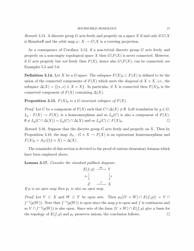
Lemma 3.17. Consider the standard pullback diagram:

E(f, p)p2−−−→ Y

p1

y ypZ

f−−−→ XIf p is an open map then p1 is also an open map.

Proof. Let V ⊂ X and W ⊂ Y be open sets. Then p1((V × W ) ∩ E(f, p)) = V ∩f−1(p(W )). Note that f−1(p(W )) is open since the map p is open and f is continuous and

so V ∩ f−1(p(W )) is also open. Since sets of the form (V ×W ) ∩ E(f, p) give a basis for

the topology of E(f, p) and p1 preserves unions, the conclusion follows. �


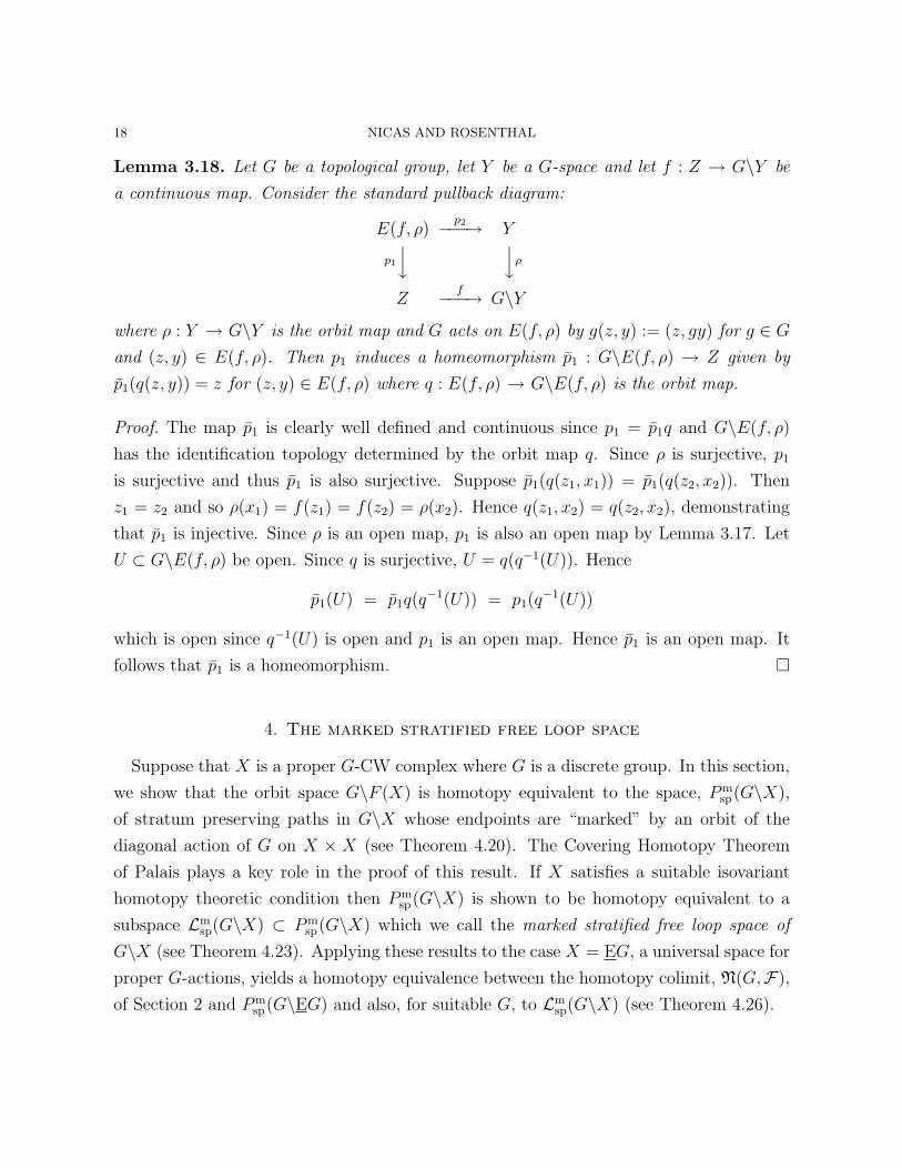
Lemma 3.18. Let G be a topological group, let Y be a G-space and let f : Z → G\Y be

a continuous map. Consider the standard pullback diagram:

E(f, ρ)p2−−−→ Y

p1

y yρZ

f−−−→ G\Y

where ρ : Y → G\Y is the orbit map and G acts on E(f, ρ) by g(z, y) := (z, gy) for g ∈ Gand (z, y) ∈ E(f, ρ). Then p1 induces a homeomorphism p1 : G\E(f, ρ) → Z given by

p1(q(z, y)) = z for (z, y) ∈ E(f, ρ) where q : E(f, ρ) → G\E(f, ρ) is the orbit map.

Proof. The map p1 is clearly well defined and continuous since p1 = p1q and G\E(f, ρ)

has the identification topology determined by the orbit map q. Since ρ is surjective, p1

is surjective and thus p1 is also surjective. Suppose p1(q(z1, x1)) = p1(q(z2, x2)). Then

z1 = z2 and so ρ(x1) = f(z1) = f(z2) = ρ(x2). Hence q(z1, x2) = q(z2, x2), demonstrating

that p1 is injective. Since ρ is an open map, p1 is also an open map by Lemma 3.17. Let

U ⊂ G\E(f, ρ) be open. Since q is surjective, U = q(q−1(U)). Hence

p1(U) = p1q(q−1(U)) = p1(q−1(U))

which is open since q−1(U) is open and p1 is an open map. Hence p1 is an open map. It

follows that p1 is a homeomorphism. �

4. The marked stratified free loop space

Suppose that X is a proper G-CW complex where G is a discrete group. In this section,

we show that the orbit space G\F (X) is homotopy equivalent to the space, Pmsp(G\X),

of stratum preserving paths in G\X whose endpoints are “marked” by an orbit of the

diagonal action of G on X × X (see Theorem 4.20). The Covering Homotopy Theorem

of Palais plays a key role in the proof of this result. If X satisfies a suitable isovariant

homotopy theoretic condition then Pmsp(G\X) is shown to be homotopy equivalent to a

subspace Lmsp(G\X) ⊂ Pm

sp(G\X) which we call the marked stratified free loop space of

G\X (see Theorem 4.23). Applying these results to the case X = EG, a universal space for

proper G-actions, yields a homotopy equivalence between the homotopy colimit, N(G,F),

of Section 2 and Pmsp(G\EG) and also, for suitable G, to Lm

sp(G\X) (see Theorem 4.26).


4.1. Orbit maps as stratified fibrations. We recall some of the basic definitions from

the theory of stratified spaces following the treatment in [11].

Definition 4.1. A partition of a topological space X consists of an indexing set J and a

collection {Xj | j ∈ J } of pairwise disjoint subspaces of X such that X =⋃j∈J Xj. For

each j ∈ J , Xj is called the j-th stratum.

A refinement of a partition {Xj | j ∈ J } of a space X is another partition {X ′i | i ∈ J ′}of X such that for every i ∈ J ′ there exists j ∈ J such that X ′i ⊂ Xj. The component

refinement of a partition {Xj | j ∈ J } of X is the refinement obtained by taking the X ′i’s

to be the connected components of the Xj’s.

Definition 4.2. A stratification of a topological space X is a locally finite partition

{Xj | j ∈ J } of X such that each Xj is locally closed in X. We say that X together

with its stratification is a stratified space.

If X is a space with a given partition then a map f : Z ×A → X is stratum preserving

along A if for each z ∈ Z, f({z} × A) lies in a single stratum of X. In particular, a map

f : Z × I → X is a stratum preserving homotopy if it is stratum preserving along I.

A class of topological spaces will mean a subclass of the class of all topological spaces,

typically defined by a property, for example, the class of all metrizable spaces.

Definition 4.3. Let X and Y be spaces with given partitions. A map p : X → Y is a

stratified fibration with respect to a class of topological spaces W if for any space Z in Wand any commutative square

Zf−−−→ X

i0

y ypZ × I H−−−→ Y

where i0(z) := (z, 0) and H is a stratum preserving homotopy, there exists a stratum

preserving homotopy H : Z × I → X such that H(z, 0) = f(z) for all z ∈ Z and pH = H.

Definition 4.4. Let X be a space with a given partition. The space of stratum preserving

paths in X, denoted by Psp(X), is the subspace of XI , the space of continuous maps of

the unit interval into X with the compact-open topology, consisting of stratum preserving

paths, i.e., paths ω : I → X such that ω(I) belongs to a single stratum of X.


Observe that a homotopy H : Z× I → X is stratum preserving if and only if its adjoint

H : Z → XI , given by H(z)(t) := H(z, t) for (z, t) ∈ Z × I, has H(Z) ⊂ Psp(X).

A group action on a space determines an invariant partition on that space as follows.

Definition 4.5 (Orbit type partition). Let G be a topological group and let X be a G-

space. For a subgroup H ⊂ G, let XH := {x ∈ X | Gx = H} where Gx is the isotropy

subgroup at x. Let (H) := {gHg−1 | g ∈ G}, the set of conjugates of H in G, and

X(H) :=⋃K∈(H) XK . Let J denote the set of conjugacy classes of subgroups of G of the

form (Gx). The subspaces X(H) are G-invariant and {X(H) | (H) ∈ J } is a partition of

X called the orbit type partition of X. Let ρ : X → G\X denote the orbit map. The set

{ρ(X(H)) | (H) ∈ J } is a partition of G\X also called the orbit type partition of G\X.

Remark 4.6. If G is a Lie group acting smoothly and properly on a smooth manifold M

then the component refinement of the orbit type partition of M is a stratification of M

which, in addition, satisfies Whitney’s Conditions A and B; see [8, Theorem 2.7.4].

An equivariant map f : X → Y between two G-spaces is isovariant if for every x ∈ X,

Gx = Gf(x). An equivariant homotopy H : X × I → Y is said to be isovariant if for each

t ∈ I, Ht := H(−, t) is isovariant.

We make use of the following version of the Covering Homotopy Theorem of Palais.

Theorem 4.7 (Covering Homotopy Theorem). Let G be a Lie group, let X be a G-space

and let Y be a proper G-space. Assume that every open subset of G\X is paracompact.

Suppose that f : X → Y is an isovariant map and that F : G\X×I → G\Y is a homotopy

such that F0 ◦ ρX = ρY ◦ f , where ρX : X → G\X and ρY : Y → G\Y are the orbit maps,

and F (ρX(X(H)) × I) ⊂ ρY (Y(H)) for every compact subgroup H ⊂ G. Then there exists

an isovariant homotopy F : X× I → Y such that F0 = f and F ◦ (ρX × idI) = ρY ◦ F . �

Remark 4.8. The Covering Homotopy Theorem (CHT) was originally demonstrated by

Palais in the case G is a compact Lie group and X and Y are second countable and locally

compact ([19, 2.4.1]). Palais later observed ([20, 4.5]) that his proof of the CHT generalizes

to the case of proper actions of a non-compact Lie group. Bredon proved the CHT under

the hypotheses that G is compact and that G\X has the property that every open subset is

paracompact ([5, II, Theorem 7.3]). A topological space is hereditarily paracompact if every

subspace is paracompact, equivalently, if every open subspace is paracompact ([16, App. I,


Lemma 8]). The class of hereditarily paracompact spaces includes all metric spaces (since

any metric space is paracompact) and all CW complexes ([16, II, sec. 4]). The authors of

[1] observed that Bredon’s proof of [5, II, Theorem 7.1], from which the CHT is deduced,

can be adapted to the case of a proper action of a non-compact Lie group; see the discussion

following [1, Theorem 1.5]. Also, note that it is not necessary to assume that the G-action

on X is proper because the induced G-action on the standard pullback E(F, ρY ) is proper

by Lemma 4.9 below.

Lemma 4.9. Suppose that G × Y → Y is a proper action of a topological group G on

a Hausdorff space Y . Let Z be a Hausdorff space and f : Z → G\Y a continuous map.

Let ρ : Y → G\Y denote the orbit map. Then the induced action of G on the standard

pullback E(f, ρ) is proper.

Proof. By hypothesis, the map AY : G × Y → Y × Y , AY (g, y) = (y, gy), is proper.

Since Z is Hausdorff, the diagonal map ∆ : Z → Z × Z is proper. The product of two

proper maps is proper and thus AY × ∆ : G × Y × Z → Y × Y × Z × Z is proper. It

follows that AZ×Y = h2 ◦ (AY × idZ) ◦ h1 : G × Z × Y → Z × Y × Z × Y is proper

where h1 : G× Z × Y → G× Y × Z and h2 : Y × Y × Z × Z → Z × Y × Z × Y are the

“interchange” homeomorphisms, h1(g, z, y) = (g, y, z) and h2(y1, y2, z1, z2) = (z1, y1, z2, y2).

Since the action of G on Y is proper, G\Y is Hausdorff ([4, III, 4.2, Proposition 3]) and so

E(f, ρ) is a closed subset of Z×Y . Hence the restriction of AZ×Y to G×E(f, ρ) is a proper

map. This restriction map factors as i◦AE(f,ρ) where i : E(f, ρ)×E(f, ρ) ↪→ Z×Y ×Z×Yis inclusion and thus AE(f,ρ) is a proper map ([4, I, 10.2, Proposition 5(d)]). �

Theorem 4.10. Suppose that G is a Lie group and that Y is a proper G-space. Let Y

and G\Y have the orbit type partitions. Then the orbit map ρ : Y → G\Y is a stratified

fibration with respect to the class of hereditarily paracompact spaces.

Proof. Let Z be a hereditarily paracompact space, let F : Z × I → G\Y be a homotopy

which is stratum preserving along I and let f : Z → Y be a map such that ρ ◦ f = F0.

Consider the standard pullback diagram:

E(F0, ρ)p2−−−→ Y

p1

y yρZ

F0−−−→ G\Y


By Lemma 3.18, p1 induces a homeomorphism p1 : G\E(F0, ρ) → Z. The map p2 is

clearly isovariant. The CHT (Theorem 4.7) implies that there is an isovariant homotopy

F : E(F0, ρ)×I → Y such that ρ◦ F = F ◦(p1× idI) and F0 = p2. Define f : Z → E(F0, ρ)

by f(z) = (z, f(z)) for z ∈ Z. Let F : Z × I → Y be given by F = F ◦ (f × idI). Then

ρ ◦ F = F and F0 = f ; furthermore, F is stratum preserving along I. �

Corollary 4.11. Suppose that G is a Lie group and that Y is a proper G-space. Let H ⊂ G

be a subgroup. Then the orbit map ρ : Y(H) → G\Y(H) is a Serre fibration.

Proof. Suppose that Z is a compact polyhedron. Then Z is metrizable and thus hereditarily

paracompact. Given a homotopy F : Z × I → G\Y(H) and a map f : Z → Y(H) such that

F0 = ρ◦f , apply Theorem 4.10 to j◦F and i◦f , where i : Y(H) ↪→ Y and j : G\Y(H) ↪→ G\Yare the inclusions, to obtain F : Z × I → Y(H) with ρ ◦ F = F and F0 = f . �

4.2. Spaces of marked stratum preserving paths. We apply the results of Section 4.1

in the case G is a discrete group to show that, for a proper G-CW complex X, the orbit

space G\F (X) is homotopy equivalent to the space, Pmsp(G\X), of stratum preserving

paths in G\X whose endpoints are “marked” by an orbit of the diagonal action of G on

X ×X; see Theorem 4.20. That theorem together with Corollaries 3.8 and 4.24 are used

to prove Theorem 4.26, which subsumes Theorem B as stated in the introduction to this

paper.

Lemma 4.12. Suppose that G is a discrete group and that Y is a proper G-space. Then

the orbit map ρ : Y → G\Y has the unique path lifting property for stratum preserving

paths, i.e., given a stratum preserving path ω : I → G\Y and y ∈ ρ−1(ω(0)) there exists a

unique path ω : I → Y such that ω(0) = y and ρ ◦ ω = ω.

Proof. Let ω : I → G\Y be a stratum preserving path, i.e., there exists a finite subgroup

H ⊂ G such that ω(I) ⊂ ρ(Y(H)) = G\Y(H). By Corollary 4.11, the restriction of ρ to

Y(H), ρ : Y(H) → G\Y(H), is a Serre fibration. The fiber over ρ(y), where y ∈ Y(H), is the

orbit G · y which is discrete since the G-action on Y is proper. By [21, 2.2 Theorem 5], a

fibration with discrete fibers has the unique path lifting property (note that in the cited

theorem, the given fibration is assumed to be a Hurewicz fibration; however, the proof of

this theorem uses only the homotopy lifting property respect to I and so remains valid for

a Serre fibration). �


Combining Theorem 4.10 and Lemma 4.12 yields:

Proposition 4.13. (Unique Lifting.) Suppose that G is a discrete group and that Y is a

proper G-space. Let Z be a hereditarily paracompact space. Suppose that F : Z×I → G\Yis stratum preserving homotopy and that f : Z → Y is a map such that ρ ◦ f = F0. Then

there exists a unique stratum preserving homotopy F : Z × I → Y such that ρ ◦ F = F

and F0 = f . �

We define a “stratified homotopy” version of F (X) as follows.

Definition 4.14. Let X be a G-space with its orbit type partition. The G-space Fsp(X)

is given by:

Fsp(X) := {(ω, y) ∈ Psp(X)×X | there exists g ∈ G such that y = gω(1)}

where G acts on Fsp(X) by the restriction of the diagonal action of G on Psp(X)×X.

Note that there is a pullback diagram

Fsp(X)i−−−→ Psp(X) × X

q

y y(ρ◦ev1)×ρ

G\X ∆−−−→ G\X ×G\X

where i is the inclusion Fsp(X) ↪→ Psp(X) × X, ρ : X → G\X is the orbit map,

ev1 : Psp(X) → X is evaluation at 1, ∆ is the diagonal map and q : Fsp(X) → G\Xis given by q((ω, y)) = ρ(y) for (ω, y) ∈ Fsp(X).

Proposition 4.15. The map ` : F (X)→ Fsp(X) given by `(x, y) = (cx, y), where cx is the

constant path at x, is an equivariant homotopy equivalence with an equivariant homotopy

inverse j : Fsp(X) → F (X) given by j(ω, y) = (ω(1), y).

Proof. Observe that j ◦ ` = idF (X). Define a homotopy, H : Fsp(X) × I → Fsp(X) by

H((ω, y), t) = (ωt, y) where ωt ∈ Psp(X) is the path ωt(s) = ω((1−s)t+s) for s ∈ I. Then

H is an equivariant homotopy from idFsp(X) to ` ◦ j. �

Corollary 4.16. The map ` : F (X) → Fsp(X) induces a homotopy equivalence¯ : G\F (X) → G\Fsp(X). �


If G is a Lie group, we say that a G-CW complex X is proper if G acts properly on X.

By [13, Theorem 1.23], a G-CW complex X is proper if and only if for each x in X the

isotropy group Gx is compact. In particular, if G is discrete, then X is a proper G-CW

complex if and only if Gx is finite for every x in X.

Proposition 4.17. Let G be a discrete group. Suppose that X is a proper G-CW complex.

Then there is a pullback diagram:

Fsp(X)q2−−−→ X × X

q1

y yρ×ρPsp(G\X)

ev0,1−−−→ G\X ×G\Xwhere ρ : X → G\X is the orbit map, q1 and q2 are given, respectively, by q1(ω, y) = ρ ◦ωand q2(ω, y) = (ω(0), y) for (ω, y) ∈ Fsp(X), and ev0,1(τ) = (τ(0), τ(1)) for τ ∈ Psp(G\X).

Proof. Let Z be a hereditarily paracompact space. Suppose h = (h0, h1) : Z → X × Xand f : Z → Psp(G\X) are maps such that ev0,1 f = (ρ× ρ)h. Let f : Z × I → G\X be

the adjoint of f , i.e., f(z, t) = f(z)(t) for (z, t) ∈ Z× I. Note that f is stratum preserving

along I. The diagram

Zh0−−−→ X

i0

y yρZ × I f−−−→ G\X

is commutative where i0(z) = (z, 0) for z ∈ Z. By Proposition 4.13, there exists a unique

F : Z × I → X which is stratum preserving along I such that ρF = f and Fi0 = h0. Let

F : Z → Psp(X) be the adjoint of F . Then Q : Z → Fsp(X) given by Q(z) = (F (z), h1(z))

for z ∈ Z is the unique map such that h = q2Q and f = q1Q. In order to conclude that

the diagram appearing in the statement of the proposition is a pullback diagram in TOP,

it suffices to show that the spaces Fsp(X) and

E(ev0,1, ρ× ρ) = {(ω, x, y) ∈ Psp(G\X)×X ×X | ω(0) = ρ(x), ω(1) = ρ(y)}

are hereditarily paracompact. Since and X and G\X are CW complexes, the main theorem

of [6] implies that the path spaces XI and (G\X)I are stratifiable in the sense of [3,

Definition 1.1] (despite the sound alike terminology, this notion of “stratifiable” is not

directly related to our Definition 4.2). It is shown in [3] that any CW complex is stratifiable,

that a countable product of stratifiable spaces is stratifiable and that a stratifiable space


is paracompact and perfectly normal, i.e., normal and every closed set is a countable

intersection of open sets. Hence XI × X and (G\X)I × X × X are stratifiable and thus

paracompact and perfectly normal. A subspace of a paracompact and perfectly normal

space is also paracompact and perfectly normal ([16, App. I, Theorem 10]). In particular,

Fsp(X) ⊂ XI ×X and E(ev0,1, ρ × ρ) ⊂ (G\X)I ×X ×X and all of their subspaces are

paracompact. �

Definition 4.18. The space Pmsp(G\X) of marked stratum preserving paths in G\X consists

of stratum preserving paths in G\X whose endpoints are “marked” by an orbit of the

diagonal action of G on X ×X. More precisely, Pmsp(G\X) = E(ev0,1, ρ× ρ) where

E(ev0,1, ρ× ρ)p2−−−→ G\(X ×X)

p1

y yρ×ρPsp(G\X)

ev0,1−−−→ G\X ×G\Xis a standard pullback diagram and ρ× ρ is induced by ρ× ρ : X ×X → G\X ×G\X.

Proposition 4.19. Let G be a discrete group. Suppose that X is a proper G-CW complex.

Then the map q : Fsp(X) → Pmsp(G\X) given by q(ω, y) = (ρ ◦ ω, ρ′(ω(0), y)), where

ρ′ : X×X → G\(X×X) is the orbit map of the diagonal action, induces a homeomorphism

q : G\Fsp(X) → Pmsp(G\X).

Proof. The pullback diagram of Proposition 4.17 factors as:

Fsp(X)q2−−−→ X × X

q

y yρ′Pm

sp(G\X)p2−−−→ G\(X ×X)

p1

y yρ×ρPsp(G\X)

ev0,1−−−→ G\X ×G\XThe outer square in the above diagram is a pullback by Proposition 4.17 and the lower

square is a pullback by definition. It follows that the upper square is a pullback. By

Lemma 3.18, q induces a homeomorphism q : G\Fsp(X) → Pmsp(G\X). �

Combining Corollary 4.16 and Proposition 4.19 yields:

Theorem 4.20. Let G be a discrete group. Suppose that X is a proper G-CW complex.

Then the map q ◦ ¯ : G\F (X) → Pmsp(G\X) is a homotopy equivalence. �


Definition 4.21. The stratified free loop space of G\X, denoted by Lsp(G\X), is the

subspace of Psp(G\X) consisting of closed paths, i.e., ω ∈ Psp(G\X) such that ω(0) = ω(1).

The marked stratified free loop space of G\X, denoted by Lmsp(G\X), is the subspace of

Pmsp(G\X) given by:

Lmsp(G\X) = {(ω, ρ′(x, y)) ∈ Pm

sp(G\X) | (x, y) ∈ F (X)0}.

(Recall that ρ : X → G\X and ρ′ : X × X → G\(X × X) are the orbit maps and

that F (X)0 is the union of the components of F (X) meeting the diagonal.) Note that if

(ω, ρ′(x, y)) ∈ Lmsp(G\X) then ω(0) = ρ(x) = ρ(y) = ω(1) and so ω ∈ Lsp(G\X).

There is a standard pullback diagram:

Lmsp(G\X)

p2−−−→ G\F (X)0

p1

y ypLsp(G\X)

ev0−−−→ G\Xwhere p is given by p(ρ′(x, y)) = ρ(x) for ρ′(x, y) ∈ G\F (X)0.

Let ∆ : G\X → G\(X × X) denote the map induced by the diagonal map,

∆ : X → X × X. Define the map ι : Lsp(G\X) → Lmsp(G\X) by ι(ω) = (ω, ∆(ω(0))).

The composite p1ι is the identity map of Lsp(G\X) and so Lsp(G\X) is homeomorphic

to a retract of Lmsp(G\X). In general, ι is not a homotopy equivalence; for example, in

the case of the infinite dihedral group, D∞, acting on R as in Example 5.5, Lsp(D∞\R) is

contractible whereas Lmsp(D∞\R) is not simply connected.

Proposition 4.22. If the discrete group G acts freely and properly on X then the map

ι : Lsp(G\X) → Lmsp(G\X) is a homeomorphism; furthermore, Lsp(G\X) = L(G\X), the

space of closed paths in G\X.

Proof. Since theG-action onX is free and proper, by Remark 3.16, F (X)0 is the diagonal of

X×X and so p : G\F (X)0→G\X is a homeomorphism. Thus p1 : Lmsp(G\X)→Lsp(G\X)

is also homeomorphism since it is a pullback of p. Hence ι = (p1)−1 is a homeomorphism.

Since the G-action is free, there is only one stratum and so Lsp(G\X) = L(G\X). �

Define S to be the image of the map G×Psp(X)→X×X given by (g, σ) 7→ (σ(0), gσ(1)).

Note that S is a G-invariant subset of X ×X and that F (X) ⊂ S.

Theorem 4.23. Suppose that the pair (S, F (X)0) can be deformed isovariantly into the

pair (F (X)0, F (X)0), i.e., there is an isovariant homotopy H : S × I → S such that


H(−, 0) is the identity of S and H(S × {1} ∪ F (X)0 × I) ⊂ F (X)0. Then the inclusion

i : Lmsp(G\X) ↪→ Pm

sp(G\X) is a homotopy equivalence.

Proof. Let H : S × I → S be an isovariant homotopy such that H(−, 0) is the identity of

S and H(S × {1} ∪ F (X)0 × I) ⊂ F (X)0. Write H = (H1, H2) where Hj : S × I → X for

j = 1, 2. Define the homotopy b : Pmsp(G\X)× I → Psp(G\X) by

b((ω, ρ′(x, y)), s)(t) =

ρ ◦H1((x, y), s− 3t) if 0 ≤ t ≤ s/3,ω( 3t−s

3−2s) if s/3 ≤ t ≤ 1− s/3,

ρ ◦H2((x, y), s+ 3t− 3) if 1− s/3 ≤ t ≤ 1.

where ρ : X → G\X and ρ′ : X × X → G\(X × X) are the orbit maps. Define the

homotopy B : Pmsp(G\X)× I → Pm

sp(G\X) by

B((ω, ρ′(x, y)), s) = (b((ω, ρ′(x, y)), s), ρ′(H((x, y), s))).

The hypotheses on H imply that B is a deformation of the pair (Pmsp(G\X),Lm

sp(G\X))

into the pair (Lmsp(G\X),Lm

sp(G\X)) and so i : Lmsp(G\X) ↪→ Pm

sp(G\X) is a homotopy

equivalence. �

The inclusion F (X)0 ↪→ S is an isovariant strong deformation retract if there is a

homotopy H : S × I → S as in Theorem 4.23 with the additional property that H is

stationary along F (X)0.

Corollary 4.24. If F (X)0 ↪→ S is an isovariant strong deformation retract then

i : Lmsp(G\X) ↪→ Pm

sp(G\X) is a homotopy equivalence. �

Remark 4.25. Suppose in Theorem 4.23 that the discrete group G acts freely and properly.

Then S = X × X and F (X)0 = ∆(X), the diagonal of X × X; see Remark 3.16. The

hypothesis of Theorem 4.23 asserts that (X ×X,∆(X)) is deformable into (∆(X),∆(X))

and so the diagonal map ∆ : X → X ×X is a homotopy equivalence. This implies that X

is contractible and hence a model for the universal space, EG, for free G-actions, provided

X has the equivariant homotopy type of a G-CW complex. Conversely, suppose that EG is

a G-CW model for the universal space such that EG×EG with the product topology and

the diagonal G-action is also a G-CW complex and has an equivariant subdivision such

that ∆(EG) is a subcomplex. Then ∆(EG) ⊂ EG×EG is an equivariant, hence isovariant

(since the G-action is free), strong deformation retract.


In Section 5 we show that the hypothesis of Corollary 4.24 is satisfied for a class of groups

which includes the infinite dihedral group and hyperbolic or euclidean triangle groups and

where X is a universal space for G-actions with finite isotropy.

Theorem 4.26. Suppose that G is a countable discrete group and that F is its fam-

ily of finite subgroups. Let EG := EFG, a universal space for proper G-actions, and

BG := G\EG.

(i) There is a homotopy equivalence N(G,F) ' Pmsp(BG).

(ii) If EG satisfies the hypothesis of Corollary 4.24 then there is a homotopy equivalence

N(G,F) ' Lmsp(BG).

Proof. Conclusion (i) of the theorem is a direct consequence of Corollary 3.8 and Theorem

4.20. Conclusion (ii) follows from (i) and Corollary 4.24. �

If G is torsion free then the family F of finite subgroups of G is the trivial family and so

|N cyc(G)| ' N(G,F) and Lmsp(BG) ∼= L(BG) (Proposition 4.22); furthermore, by Remark

4.25, Theorem 4.26(ii) applies thus recovering the familiar result |N cyc(G)| ' L(BG).

5. Examples

Let EG denote the universal space for properG-actions and BG = G\EG. In this section,

we show that if G is the infinite dihedral group or a hyperbolic or euclidean triangle group,

then the hypothesis of Corollary 4.24 is satisfied; that is, F (EG)0 ↪→ S is an isovariant

strong deformation retract. By Theorem 4.26, this implies that N(G,F) ' Pmsp(BG) '

Lmsp(BG), where F is the family of finite subgroups of G. This is accomplished by showing

that, for these groups, F (EG) is path connected and F (X) ↪→ S is a G × G-isovariant

strong deformation retract.

Let G be a discrete group and X a proper G-space. Recall that F (X) is the image of

AX : G×X → X ×X, where AX(g, x) := (x, gx) for (g, x) ∈ G×X, and S is the image

of the map G× Psp(X) → X ×X given by (g, σ) 7→ (σ(0), gσ(1)). Notice that F (X) and

S are each G × G-invariant subsets of X ×X. Let ρ : X → G\X denote the orbit map.

Then F (X) = (ρ× ρ)−1(∆(G\X)), and S = (ρ× ρ)−1({(σ(0), σ(1)) | σ ∈ Psp(G\X)}) by

Lemma 4.12.


Proposition 5.1. Let G be a discrete group and X a proper G-space. Assume that G\Xis homeomorphic to a subset of Rn for some n, and that the images of the strata of G\Xin Rn are convex. Then F (X) ↪→ S is a G×G-isovariant strong deformation retract.

Proof. Let h be a homeomorphism from G\X to D ⊂ Rn such that the images of the

strata of G\X under h are convex. Define H ′ : Rn × Rn × I → Rn × Rn by H ′((a, b), t) =

(a, ta + (1 − t)b). Notice that H ′(a, a, t) = (a, a) for every a ∈ Rn and every t ∈ I. Let

S = {(σ(0), σ(1)) | σ ∈ Psp(G\X)}, and let H = (h×h)−1 ◦H ′ ◦((h×h)|S× idI). Since the

images of the strata of G\X under h are convex, H : S × I → S is a homotopy such that

H0 ◦ (ρ× ρ)|eS = (ρ× ρ)|eS ◦ ideS and H((ρ× ρ)(S(K×Kg))× I) ⊂ (ρ× ρ)(S(K×Kg)) for every

finite subgroup K of G and every g ∈ G. Observe that if (x, y) ∈ S, then (G × G)(x,y) =

Gx × Gy = K ×Kg for some finite subgroup K of G and some g ∈ G. Therefore, by the

Covering Homotopy Theorem (Theorem 4.7), there exists a G × G-isovariant homotopy

H : S × I → S covering H such that H0 = ideS. Since (ρ × ρ)−1(∆(G\X)) = F (X) it

follows that H1(S) ⊂ F (X). Thus, H is the desired homotopy. �

Corollary 5.2. Let G be a discrete group and X a proper G-space. Assume that G\Xis homeomorphic to a subset of Rn for some n, and that the images of the strata of G\Xin Rn are convex. If F (X) is path connected, then F (X)0 = F (X) ↪→ S is an isovariant

strong deformation retract.

Next we determine when F (X) is path connected.

Theorem 5.3. Let G be a discrete group and X a path connected G-space. Then, F (X)

is path connected if every element of G can be expressed as a product of elements each of

which fixes some point in X. If, in addition, G acts properly on X, then the converse is

true.

Proof. Let S = {s ∈ G | sy = y for some y ∈ X}. Clearly, if s ∈ S and y ∈ X such

that sy = y, then AX(s, y) = AX(1, y). Since X is path connected, this implies that

AX(S ×X) ⊂ F (X) is path connected.

Suppose S generates G. Let (g, x) ∈ G×X be given. We will show that there is a path

in F (X) connecting AX(g, x) to a point in AX(S×X). Write g = sn · · · s2s1, where si ∈ S.

For each i, there is an xi ∈ X such that sixi = xi. Therefore,

AX(g, x1) = AX(gs−11 , x1), and AX(gs−1

1 · · · s−1i , xi+1) = AX(gs−1

1 · · · s−1i+1, xi+1)


for each i, 1 ≤ i ≤ n− 1. Since X is path connected, AX({h} ×X) is path connected for

every h ∈ G. Thus, AX(g, x) and AX(1, xn) are connected by a path in F (X).

Now assume that G acts properly on X, and F (X) is path connected. Let N be the

subgroup of G generated by S. Since S is closed under conjugation, N is a normal subgroup

of G. Therefore, G/N acts on N\X by gN · ρ(x) = ρ(gx), where ρ : X → N\X is the

orbit map. It is easy to check that the action is free. The fact that G acts properly

on X implies that N acts properly on X and that X is Hausdorff; furthermore, N\X is

Hausdorff [4, III, 4.2, Proposition 3]. Recall that a discrete group G acts properly on a

Hausdorff space X if and only if for every pair of points x, y ∈ X, there is a neighborhood

Vx of x and a neighborhood Vy of y such that the set of all g ∈ G for which gVx ∩Vy 6= ∅ is

finite [4, III, 4.4, Proposition 7]. This implies that G/N acts properly on N\X. Therefore,

AG/N : G/N ×N\X → N\X×N\X is a homeomorphism onto its image F (N\X). Thus,

F (N\X) is path connected if and only if G/N is trivial. Since the map ρF : F (X) →F (N\X), defined by ρF (x, gx) = (ρ(x), ρ(gx)), is onto and F (X) is path connected, it

follows that G/N is trivial. That is, G = N . �

An immediate consequence of this theorem is the following.

Corollary 5.4. Let G be a discrete group and F a family of subgroups of G. If there exists

a set of generators, S of G, with the property that for every s ∈ S, there is an H ∈ F such

that s ∈ H, then F (EFG) is path connected.

Example 5.5 (The infinite dihedral group). Let G = D∞ = 〈a, b | a2 = 1, aba−1 = b−1〉and X = R, where a acts by reflection through zero and b acts by translation by 1. Since

R is a model for ED∞ and D∞ is generated by two elements of order two, namely a and

ab, F (R) is path connected by Corollary 5.4. The quotient of R by D∞ is homeomorhpic

to the closed interval [0, 12]. The strata are {0}, {1

2} and (0, 1

2). Therefore, Corollary 5.2

implies that F0(R) ↪→ S is an isovariant strong deformation retract.

Example 5.6 (Triangle groups). Let

G = 〈a, b, c | a2 = b2 = c2 = (ab)p = (bc)q = (ca)r = 1〉,

where p, q, r are natural numbers such that 1p

+ 1q

+ 1r≤ 1. The group G can be realized

as a group of reflections through the sides of a euclidean or hyperbolic triangle whose

interior angles measure πp, πq

and πr, where the generators a, b and c act by reflections


through the corresponding sides. Thus, the triangle group G produces a tessellation of

the euclidean or hyperbolic plane by these triangles. Therefore, this plane is a model for

EG, whose quotient, D, is equivalent to the given triangle. By Corollary 5.4, F (EG) is

path connected. There are seven strata of D, namely D, Sa, Sb, Sc, and each of the three

vertices, where D denotes the interior of D, and Sa, Sb, and Sc are the interiors of the sides

of the triangle, Sa, Sb, and Sc, respectively, through which a, b, and c reflect. It follows

from Corollary 5.2 that F0(EG) ↪→ S is an isovariant strong deformation retract.

Remark 5.7. Let X be a G-space and Y an H-space. Clearly, FG×H(X × Y ) ∼= FG(X) ×FH(Y ), and FG×H(X ×Y )0

∼= FG(X)0×FH(Y )0. (Here, the group that is acting has been

added to the notation of the configuration space.) Furthermore, since (x, y) and (x′, y′)

are in the same stratum of X × Y if and only if x and x′ are in the same stratum of X

and y and y′ are in the same stratum of Y , it follows that SX×Y ∼= SX × SY . Therefore, if

FG(X)0 ↪→ SX is a G-isovariant strong deformation retraction and FH(Y )0 ↪→ SY is an H-

isovariant strong deformation retraction, then FG×H(X×Y )0 ↪→ SX×Y is a G×H-isovariant

strong deformation retraction. This observation produces interesting examples for which

Theorem 4.26 is true. If X = R, G = Z, Y = R and H = D∞, then FZ×D∞(R × R) ∼=FZ(R) × FD∞(R) is not path connected, since FZ(R) is not path connected. Moreover,

FZ×D∞(R×R)0 6= ∆(R) and FZ×D∞(R×R)0 6= FZ×D∞(R×R). Despite this, Theorem 4.26

applies to Z×D∞.

6. A Comparison of G\F (EG) and G\F (EG)

In this section we examine the map N(G, {1})→ N(G,F), where G is a discrete group

and F is the family of finite subgroups of G. This enables us to compute the induced map

HH∗(ZG)→ HHF∗ (ZG).

Let E be a model for EG and E be a model for the universal space for proper G-actions.

Then, G\F (E) is homeomorphic to N(G, {1}), and N(G,F) is homeomorphic to G\F (E)

by Corollary 3.7. The universal property of E implies that there is a G-equivariant map,

f : E → E, that is unique up to G-homotopy equivalence. Then F (f) : F (E) → F (E)

induces a map f : G\F (E) → G\F (E). Note that for a different choice of f , the induced

map will be homotopy equivalent to f . The corresponding map on homology groups is

denoted f∗ : HH∗(ZG)→ HHF∗ (ZG). Recall that

AE : G\(G× E)→ G\F (E)


is a homeomorphism, since G acts freely and properly on E (Proposition 3.10). By Propo-

sition 3.11, there is a homeomorphism

h :∐

C(g)∈conj(G)

Z(g)\E→ G\(G× E),

which sends the orbit Z(g) · x to the orbit G · (g, x). This produces a map

φ :∐

C(g)∈conj(G)

Z(g)\E→ G\F (E),

where φ = f ◦ AE ◦ h. That is, the image of Z(g) · x under φ is G · (f(x), g · f(x)), where

g is in G and x is in E. Thus, we have the following commutative diagram.

HH∗(ZG)f∗ // HHF∗ (ZG)

⊕C(g)∈conj(G)

H∗(BZ(g); Z)

φ∗

66nnnnnnnnnnnn∼=

OO

IfH is a finite group, then the Sullivan Conjecture, proved by Miller [17], implies that a map

from BH to a finite dimensional CW complex is null homotopic. If E is finite dimensional,

then F (E) is homotopy equivalent to a finite dimensional CW complex. Thus, if Z(g) is

finite, then the image of H∗((BZ(g); Z) under φ∗ is zero.

For an illustrative example, consider the infinite dihedral group, D∞ = 〈a, b | a2 =

1, aba−1 = b−1〉. Let E = R, where a acts by reflection through zero and b acts by

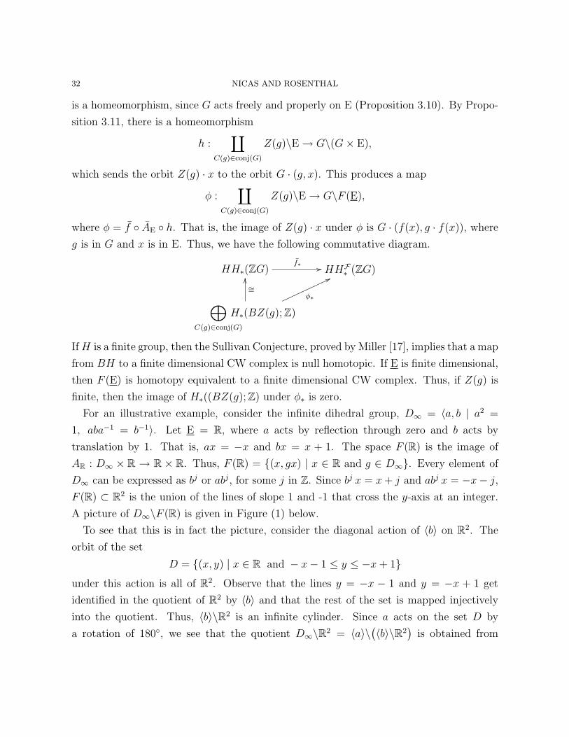
translation by 1. That is, ax = −x and bx = x + 1. The space F (R) is the image of

AR : D∞ × R → R × R. Thus, F (R) = {(x, gx) | x ∈ R and g ∈ D∞}. Every element of

D∞ can be expressed as bj or abj, for some j in Z. Since bj x = x+ j and abj x = −x− j,F (R) ⊂ R2 is the union of the lines of slope 1 and -1 that cross the y-axis at an integer.

A picture of D∞\F (R) is given in Figure (1) below.

To see that this is in fact the picture, consider the diagonal action of 〈b〉 on R2. The

orbit of the set

D = {(x, y) | x ∈ R and − x− 1 ≤ y ≤ −x+ 1}

under this action is all of R2. Observe that the lines y = −x − 1 and y = −x + 1 get

identified in the quotient of R2 by 〈b〉 and that the rest of the set is mapped injectively

into the quotient. Thus, 〈b〉\R2 is an infinite cylinder. Since a acts on the set D by

a rotation of 180◦, we see that the quotient D∞\R2 = 〈a〉\(〈b〉\R2

)is obtained from


......

· ·

· ·

· ·

· ·

· ·

Figure 1. The space D∞\F (R).

{(x, y) ∈ D | y ≥ x} by identifying the endpoints of the line segments y = x + t, where

t ≥ 0 (that is, the points (−t−12, t−1

2) and (−t+1

2, t+1

2)), as well as by identifying the points

(x, x) and (−x,−x), where −1/2 ≤ x ≤ 1/2. Thus, D∞\R2 looks like an “infinite chisel”,

and D∞\F (R) ⊂ D∞\R2 is as shown above.

The non-trivial finite subgroups of D∞ are of the form 〈abi〉, where i ∈ Z. For each i,

〈abi〉 fixes −i/2 ∈ R. Beginning with the action of D∞ on R, construct a model for ED∞

by replacing each half-integer with an S∞. Denote this “string of pearls” model for ED∞

by E, and let f : E → E be the equivariant map that collapses each S∞ to a point. The

conjugacy classes of D∞ are:

C(1) = {1}

C(a) = {ab2i : i ∈ Z}

C(ab) = {ab2i+1 : i ∈ Z}

C(bj) = {bj, b−j}, j ∈ N.

The corresponding centralizers are

Z(1) = D∞

Z(a) = {1, a}

Z(ab) = {1, ab}

Z(bj) = 〈b〉, j ∈ N.


Note that D∞\E is an “interval” with an RP∞ at each end; 〈a〉\E is a “ray” that begins

with an RP∞ at 0 and has an S∞ at every positive half-integer; 〈ab〉\E is a “ray” that

begins with an RP∞ at 1/2 and has an S∞ at every other positive half-integer; and Z\Eis a “circle” with two S∞’s in place of vertices.

The image of φ is broken into the pieces

φ(D∞ · x) = D∞ · (f(x), f(x))(4)

φ(Z(a) · x) = D∞ · (f(x),−f(x))(5)

φ(Z(ab) · x) = D∞ · (f(x),−f(x)− 1)(6)

φ(Z(bj) · x) = D∞ · (f(x), f(x) + j),(7)

where j is a positive integer and x ∈ E. Referring to diagram (1), the base of D∞\F (E) is

(4), the pieces (5) and (6) are the sides of D∞\F (E), and (7) provides each of the circles.

Therefore, φ is a gluing of the disjoint pieces, Z(g)\E, after each S∞ and each RP∞, is

collapsed to a point. Observe that,

HH∗(ZD∞) ∼= H∗(BD∞; Z)⊕H∗(BZ(a); Z)⊕H∗(BZ(ab); Z)⊕⊕j>0

H∗(BZ(bj); Z).

Since Z(a) ∼= Z/2 ∼= Z(ab), the Sullivan Conjecture implies that the image of H∗(BZ(a); Z)

and H∗(BZ(ab); Z) under φ∗ is zero. By the above analysis, φ(BD∞) = D∞\R ∼= [0, 1].

Therefore, the image of Hi(BD∞; Z) under φi is 0, for i ≥ 1. The rest of HHi(ZD∞) is

mapped injectively into HHFi (ZD∞), i ≥ 1.

Classical Hochschild homology has been used to study the K-theory of groups rings

via the Dennis trace, dtr : K∗(RG) → HH∗(RG). In [15], Luck and Reich were able to

determine how much of K∗(ZG) is detected by the Dennis trace. A natural question is to

determine the composition of the Dennis trace with the map f∗ : HH∗(ZG)→ HHF∗ (ZG).

From Luck and Reich, we have the following commutative diagram

HG∗ (E; KZ)

��

A // K∗(ZG)

dtr��

HG∗ (E; HHZ)

B // HH∗(ZG)

[15, p.595], where the maps A and B are assembly maps in the equivariant homology

theories with coefficients in the connective algebraic K-theory spectrum, KZ, associated

to Z, and the Hochschild homology spectrum HHZ, respectively. Each assembly map is


induced by the collapse map E → pt. Luck and Reich use the composition of the Dennis

trace with the assembly map in algebraic K-theory, dtr ◦ A, to achieve their detection

results. In particular, they observe that the assembly map in Hochschild homology factors

as

HG∗ (EG; HHZ)

B // HH∗(ZG)

⊕C(g)∈conj(G)〈g〉∈F

H∗(BZ(g); Z)

∼=

OO

� � //

⊕C(g)∈conj(G)

H∗(BZ(g); Z)

∼=

OO

[15, p. 630]. Given the discussion above, in the case G = D∞,

HG∗ (ED∞; HHZ) ∼= H∗(BD∞; Z)⊕H∗(BZ(a); Z)⊕H∗(BZ(ab); Z).

Therefore, f∗ ◦B = 0, which implies that the image of f∗ ◦ dtr ◦ A is zero.

We conclude with speculation about a possible geometric application of the groups

HHF∗ (ZG). Associated to a parametrized family of self-maps of a manifold M , there are

geometrically defined “intersection invariants,” in particular, the framed bordism invariants

of Hatcher and Quinn [10], which take values in abelian groups that are known to be related

to the Hochschild homology groups HH∗(ZG), where G is the fundamental group of M [9].

It appears plausible that the groups HHF∗ (ZG), where F is the family of finite subgroups,

could play an analogous role in the yet to be developed homotopical intersection theory of

orbifolds.

References

[1] R. Ayala, F.F. Lasheras, A. Quintero, The equivariant category of proper G-spaces, Rocky MountainJ. Math. 31 (2001), 1111–1132.

[2] H. Biller, Characterizations of proper actions, Math. Proc. Camb. Phil. Soc. 136 (2004), 429–439.[3] C.J.R. Borges, On stratifiable spaces, Pacific J. Math. 17 (1966), 1–16.[4] N. Bourbaki, Elements of Mathematics: General Topology, Part I (English edition), Addison Wesley,

Reading MA, 1966.[5] G.E. Bredon, Introduction to Compact Transformation Groups, Academic Press, New York, 1972.[6] R. Cauty, Sur les espaces d’applications dans les CW-complexes, Arch. Math. (Basel) 27 (1976),

306–311.[7] J. Davis and W. Luck, Spaces over a category and assembly maps in isomorphism conjectures in K-

and L-theory, K-theory 15 (1998), 201-252.[8] J.J. Duistermaat and J.A.C Kolk, Lie groups, Springer-Verlag, Berlin, 2000.[9] R. Geoghegan and A. Nicas, Parametrized Lefschetz-Nielsen fixed point theory and Hochschild homol-

ogy traces, Amer. J. Math. 116 (1994), 397–446.


[10] A. Hatcher and F. Quinn, Bordism invariants of intersections of submanifolds, Trans. Amer. Math.Soc. 200 (1974), 327–344.

[11] B. Hughes, Stratified path spaces and fibrations, Proc. Roy. Soc. Edinburgh 129A (1999), 351–384.[12] J.-L. Loday, Cyclic homology, second ed., Springer-Verlag, New York, NY, 1998.[13] W. Luck, Transformation Groups and Algebraic K-Theory, Lecture Notes in Mathematics vol. 1408,

Springer-Verlag, Berlin, 1989.[14] W. Luck, Survey on classifying spaces for families of subgroups. In Infinite groups: geometric, com-

binatorial and dynamical aspects, vol. 248 of Progr. Math., Birkhauser, Basel, 2005, pp. 269-322.[15] W. Luck and H. Reich, Detecting K-theory by cyclic homology, Proc. London Math. Soc. (3) 93

(2006), 593–634.[16] A.T. Lundell and S. Weingram, The Topology of CW Complexes, Van Nostrand Reinhold Co., New

York, 1969.[17] H. Miller, The Sullivan conjecture on maps from classifying spaces, Ann. of Math. 120 (1984), 39–87.[18] J. Milnor, Construction of universal bundles, I, Ann. of Math. 63 (1956), 272–284.[19] R.S. Palais, The classification of G-spaces, Mem. Amer. Math. Soc., No. 36, 1960.[20] R.S. Palais, On the existence of slices for actions of non-compact Lie groups, Ann. of Math. 73 (1961),

295–323.[21] E.H. Spanier, Algebraic Topology, McGraw-Hill, New York, 1966.[22] R. Talbert, An isomorphism between Bredon and Quinn homology, Forum Math. 11 (1999), 591-616.

Department of Mathematics and Statistics, McMaster University, Hamilton, Ontario,Canada L8S 4K1

E-mail address: [email protected]

Department of Mathematics and Computer Science, St. Johns University, 8000 UtopiaPkwy, Jamaica, NY 11439, USA

E-mail address: [email protected]

introduction - st. john's university

Documents