introduction modeling nancial assets
TRANSCRIPT

SCALING AND MULTISCALING IN FINANCIAL SERIES
A SIMPLE MODEL
ALESSANDRO ANDREOLI FRANCESCO CARAVENNA PAOLO DAI PRA AND GUSTAVO POSTA
Abstract We propose a simple stochastic volatility model which is analytically tractablevery easy to simulate and which captures some relevant stylized facts of financial assetsincluding scaling properties In particular the model displays a crossover in the log-returndistribution from power-law tails (small time) to a Gaussian behavior (large time) slowdecay in the volatility autocorrelation and multiscaling of moments Despite its few param-eters the model is able to fit several key features of the time series of financial indexessuch as the Dow Jones Industrial Average with a remarkable accuracy
1 Introduction
11 Modeling financial assets Recent developments in stochastic modelling of time se-ries have been strongly influenced by the analysis of financial assets such as exchange ratesstocks and market indexes The basic model that has given rise to the celebrated Blackamp Scholes formula [22 23] assumes that the logarithm Xt of the price of the asset aftersubtracting the trend evolves through the simple equation
dXt = σ dBt (11)
where σ (the volatility) is a constant and (Bt)tge0 is a standard Brownian motion It hasbeen well-know for a long time that despite its success this model is not consistent with anumber of stylized facts that are empirically detected in many real time series eg
bull the volatility is not constant and may exhibit high peaks that may be interpreted asshocks in the market
bull the empirical distribution of the increments Xt+h minusXt of the logarithm of the pricemdash called log-returns mdash is non Gaussian displaying power-law tails (see Figure 4(b)below) especially for small values of the time span h while a Gaussian shape isapproximately recovered for large values of h
bull log-returns corresponding to disjoint time-interval are uncorrelated but not indepen-dent in fact the correlation between the absolute values |Xt+hminusXt| and |Xs+hminusXs|mdash called volatility autocorrelation mdash is positive (clustering of volatility) and has aslow decay in |t minus s| (long memory) at least up to moderate values for |t minus s| (cfFigure 3(b)-(c) below)
In order to account for these facts a very popular choice in the literature of mathematicalfinance and financial economics has been to upgrade the basic model (11) allowing σ = σtto vary with t and to be itself a stochastic process This produces a wide class of processes
Date January 20 20122010 Mathematics Subject Classification 60G44 91B25 91G70Key words and phrases Financial Index Time Series Scaling Multiscaling Brownian Motion Stochastic
Volatility Heavy Tails Multifractal ModelsWe gratefully acknowledge the support of the University of Padova under grant CPDA08210508
1
2 ALESSANDRO ANDREOLI FRANCESCO CARAVENNA PAOLO DAI PRA AND GUSTAVO POSTA
minus003 minus002 minus001 000 001 002 003
010
2030
4050
60
1 day2 days5 days10 days25 days
(a) Diffusive scaling of log-returns
0 1 2 3 4 5
00
05
10
15
20
25
(b) Multiscaling of moments
Figure 1 Scaling properties of the DJIA time series (opening prices 1935-2009)(a) The empirical densities of the log-returns over 1 2 5 10 25 days show a re-markable overlap under diffusive scaling(b) The scaling exponent A(q) as a function of q defined by the relation mq(h) asymphA(q) (cf (14)) bends down from the Gaussian behavior q2 (red line) for q geq 3 The quantity A(q) is evaluated empirically through a linear interpolation of(logmq(h)) versus (log h) for h isin 1 5 (cf section 7 for more details)
known as stochastic volatility models determined by the process (σt)tge0 which are ableto capture (at least some of) the above-mentioned stylized facts cf [6 29] and referencestherein
More recently other stylized facts have been pointed out concerning the scaling propertiesof the empirical distribution of the log-returns Given a daily time series (si)1leileT over aperiod of T 1 days denote by ph the empirical distribution of the (detrended) log-returnscorresponding to an interval of h days
ph(middot) =1
T minus h
Tminushsumi=1
δxi+hminusxi(middot) xi = log(si)minus di (12)
where di is the local rate of linear growth of log(si) (see section 7 for details) and δx(middot)denotes the Dirac measure at x isin R The statistical analysis of various financial series suchas the Dow Jones Industrial Average (DJIA) or the Nikkei 225 shows that for small valuesof h ph obeys approximately a diffusive scaling relation (cf Figure 1(a))
ph(dr) 1radichg
(rradich
)dr (13)
where g is a probability density with power-law tails Considering the q-th empirical momentmq(h) defined by
mq(h) =1
T minus h
Tminushsumi=1
|xi+h minus xi|q =
int|r|q ph(dr) (14)
from relation (13) it is natural to guess that mq(h) should scale as hq2 This is indeed whatone observes for moments of small order q le q (with q 3 for the DJIA) However for
SCALING AND MULTISCALING IN FINANCIAL SERIES 3
moments of higher order q gt q the different scaling relation hA(q) with A(q) lt q2 takesplace cf Figure 1(b) This is the so-called multiscaling of moments cf [32 21 20 17]
An interesting class of models that are able to reproduce the multiscaling of moments mdashas well as many other features notably the persistence of volatility on different time scales mdashare the so-called multifractal models like the MMAR (Multifractal Model of Asset Returnscf [14]) and the MSM (Markov-Switching Multifractal cf [13]) These models describethe evolution of the detrended log-price (Xt)tge0 as a random time-change of Brownianmotion Xt = WI(t) where the time-change (I(t))tge0 is a continuous and increasing processsometimes called trading time which displays multifractal features and is usually taken tobe independent of the Brownian motion (Wt)tge0 (cf [12] for more details)
Modeling financial series through a random time-change of Brownian motion is a classi-cal topic dating back to Clark [15] and reflects the natural idea that external informationinfluences the speed at which exchanges take place in a market It should be stressed thatunder the mild regularity assumption that the time-change (I(t))tge0 has absolutely contin-uous paths as any random time-change of Brownian motion Xt = WI(t) can be written as
a stochastic volatility model dXt = σt dBt and viceversa1 However a key feature of mul-tifractal models is precisely that their trading time (I(t))tge0 has non absolutely continuouspaths as hence they cannot be expressed as stochastic volatility models This makes theiranalysis harder as the standard tools available for Ito diffusions cannot be applied
The purpose of this paper is to define a simple stochastic volatility model mdash or equiv-alently an independent random time change of Brownian motion where the time-changeprocess has absolutely continuous paths mdash which agrees with all the above mentioned styl-ized facts displaying in particular a crossover in the log-return distribution from a power-lawto a Gaussian behavior slow decay in the volatility autocorrelation diffusive scaling andmultiscaling of moments In its most basic version the model contains only three real pa-rameters and is defined as a simple deterministic function of a Brownian motion and anindependent Poisson process This makes the process analytically tractable and very easyto simulate Despite its few degrees of freedom the model is able to fit remarkably wellseveral key features of the time series of the main financial indexes such as DJIA SampP 500FTSE 100 Nikkei 225 In this paper we present a detailed numerical analysis on the DJIA
Let us mention that there are subtler stylized facts that are not properly accounted by ourmodel such as the multi-scale intermittency of the volatility profile the possible skewnessof the log-return distribution and the so-called leverage effect (negative correlation betweenlog-returns and future volatilities) cf [16] As we discuss in section 3 such features mdashthat are relevant in the analysis of particular assets mdash can be incorporated in our modelin a natural way Generalizations in this sense are currently under investigation as are theperformances of our model in financial problems like the pricing of options (cf A AndrelolirsquosPhD Thesis [2]) In this article we stick for simplicity to the most basic formulation
Finally although we work in the framework of stochastic volatility models we point outthat an important alternative class of models in discrete time widely used in the econometricliterature is given by autoregressive processes such as ARCH GARCH FIGARCH and their
1More precisely ldquoindependent random time changes of Brownian motion with absolutely continuous time-changerdquo mdash that is processes (Xt)tge0 such that Xt minusX0 = WI(t) where (Wt)tge0 is a Brownian motion and(I(t))tge0 is an independent process with increasing and absolutely continuous paths as mdash and ldquostochasticvolatility models with independent volatilityrdquo mdash that is processes (Xt)tge0 such that dXt = σt dBt where(Bt)tge0 is a Brownian motion and (σt)tge0 is an independent process with paths in L2
loc(R) as mdash are the sameclass of processes cf [6 29] The link between the two representations dXt = σt dBt and Xt minusX0 = WI(t)
is given by σt =radicI prime(t) and Bt =
int t0
(I prime(s))minus12dWI(s) =int It0
(I prime(Iminus1(v)))minus12dWu
4 ALESSANDRO ANDREOLI FRANCESCO CARAVENNA PAOLO DAI PRA AND GUSTAVO POSTA
generalizations cf [18 8 5 9] More recently continuous-time versions have been studied aswell cf [24 25] With no aim for completeness let us mention that GARCH and FIGARCHdo not display multiscaling of moments cf [12 sect814] We have also tested the modelrecently proposed in [10] which is extremely accurate to fit the statistics of the empiricalvolatility and it does exhibit multiscaling of moments The price to pay is however thatthe model requires the calibration of more than 30 parameters
We conclude noting that long memory effects in autoregressive models are obtainedthrough a suitable dependence on the past in the equation for the volatility while largeprice variations are usually controlled by specific features of the driving noise In our modelwe propose a single mechanism modeling the reaction of the market to shocks which is thesource of all the mentioned stylized facts
12 Content of the paper The paper is organized as follows
bull In section 2 we give the definition of our model we state its main properties and wediscuss its ability to fit the DJIA time series in the period 1935-2009
bull In section 3 we discuss some key features and limitations of our model point outpossible generalizations and compare it with other models
bull Sections 4 5 and 6 contain the proofs of the main results plus some additional mate-rial
bull In section 7 we discuss more in detail the numerical comparison between our modeland the DJIA time series
bull Finally appendix A contains the proof of some technical results while appendix B isdevoted to a brief discussion of the model introduced by F Baldovin and A Stellain [7 31] which has partially inspired the construction of our model
13 Notation Throughout the paper the indexes s t u x λ run over real numbers whilei km n run over integers so that t ge 0 means t isin [0infin) while n ge 0 means n isin 0 1 2 The symbol ldquosimrdquo denotes asymptotic equivalence for positive sequences (an sim bn if and onlyif anbn rarr 1 as n rarr infin) and also equality in law for random variables like W1 sim N (0 1)Given two real functions f(x) and g(x) we write f = O(g) as xrarr x0 if there exists M gt 0such that |f(x)| le M |g(x)| for x in a neighborhood of x0 while we write f = o(g) iff(x)g(x) rarr 0 as x rarr x0 in particular O(1) (resp o(1)) is a bounded (resp a vanishing)quantity The standard exponential and Poisson laws are denoted by Exp(λ) and Po(λ)for λ gt 0 X sim Exp(λ) means that P (X le x) = (1 minus eminusλx)1[0infin)(x) for all x isin R while
Y sim Po(λ) means that P (Y = n) = eminusλλnn for all n isin 0 1 2 We sometimes write(const) to denote a positive constant whose value may change from place to place
2 The model and the main results
We introduce our model as an independent random time change of a Brownian motionin the spirit eg of [15] and [4] An alternative and equivalent definition as a stochasticvolatility model is illustrated in section 22
21 Definition of the model In its basic version our model contains only three realparameters
bull λ isin (0+infin) is the inverse of the average waiting time between ldquoshocksrdquo in the market
bull D isin (0 12] determines the sub-linear time change t 7rarr t2D which expresses theldquotrading timerdquo after shocks
SCALING AND MULTISCALING IN FINANCIAL SERIES 5
bull σ isin (0+infin) is proportional to the average volatility
In order to have more flexibility we actually let σ be a random parameter ie a positiverandom variable whose distribution ν becomes the relevant parameter
bull ν is a probability on (0infin) connected to the volatility distribution
Remark 1 When the model is calibrated to the main financial indexes (DJIA SampP 500FTSE 100 Nikkei 225) the best fitting turns out to be obtained for a nearly constant σIn any case we stess that the main properties of the model are only marginally dependenton the law ν of σ in particular the first two moments of ν ie E(σ) and E(σ2) areenough to determine the features of our model that are relevant for real-world times seriescf Remark 10 below Therefore roughly speaking we could say that in the general case ofrandom σ our model has four ldquoeffectiverdquo real parameters
Beyond the parameters λD ν we need the following three sources of alea
bull a standard Brownian motion W = (Wt)tge0
bull a Poisson point process T = (τn)nisinZ on R with intensity λ
bull a sequence Σ = (σn)nge0 of independent and identically distributed positive randomvariables with law ν (so that σn sim ν for all n) and for conciseness we denote by σ avariable with the same law ν
We assume that W T Σ are defined on some probability space (ΩF P ) and that they areindependent By convention we label the points of T so that τ0 lt 0 lt τ1 We will actuallyneed only the points (τn)nge0 and we recall that the random variables (minusτ0) τ1 (τn+1minusτn)nge1
are independent and identically distributed with marginal laws Exp(λ) In particular 1λ isthe mean distance between the points in T except for τ0 and τ1 whose average distance is2λ Although some of our results would hold for more general distributions of T we stickfor simplicity to the (rather natural) choice of a Poisson process
For t ge 0 we define
i(t) = supn ge 0 τn le t = T cap (0 t] (21)
so that τi(t) is the location of the last point in T before t Plainly i(t) sim Po(λt) Then weintroduce the basic process I = (It)tge0 defined by
It = I(t) = σ2i(t)
(tminus τi(t)
)2D+
i(t)sumk=1
σ2kminus1 (τk minus τkminus1)2D minus σ2
0 (minusτ0)2D (22)
with the agreement that the sum in the right hand side is zero if i(t) = 0 More explicitly(It)tge0 is a continuous process with I0 = 0 and Iτn+hminusIτn = (σ2
n)h2D for 0 le h le (τn+1minusτn)
We note that the derivative ( ddtIt)tge0 is a stationary regenerative process cf [3] See Figure 2
for a sample trajectory of (It)tge0 when D lt 12
We then define our model X = (Xt)tge0 by setting
Xt = WIt (23)
In words our model is an random time change of the Brownian motion (Wt)tge0 throughthe time-change process (It)tge0 Note that I is a strictly increasing process with absolutelycontinuous paths and it is independent of W
When D = 12 and σ is constant we have It = σ2t and the model reduces to Black amp
Scholes with volatility σ On the other hand when D lt 12 the paths of I are singular (non
differentiable) at the points in T cf Figure 2 This suggests a possible financial interpretation
6 ALESSANDRO ANDREOLI FRANCESCO CARAVENNA PAOLO DAI PRA AND GUSTAVO POSTA
τ1 τ2 τ3τ0
It
t
Figure 2 A sample trajectory of the process (It)tge0
of the instants in T as the epochs at which big shocks arrive in the market making thevolatility jump to infinity This will be more apparent in next subsection where we give astochastic volatility formulation of the model We point out that the singularity is producedby the sub-linear time change t 7rarr t2D that was first suggested by F Baldovin and A Stellain [7 31] (their model is described in appendix B)
22 Basic properties Let us state some basic properties of our model that will be provedin section 6
(A) The process X has stationary increments
(B) The following relation between moments of Xt and σ holds for any q gt 0
E(|Xt|q) ltinfin for some (hence any) t gt 0 lArrrArr E(σq) ltinfin (24)
(C) The process X can be represented as a stochastic volatility model
dXt = vt dBt (25)
where (Bt)tge0 is a standard Brownian motion and (vt)tge0 is an independent process
defined by (denoting I prime(s) = ddsI(s))
Bt =
int t
0
1radicI prime(s)
dWI(s) =
int It
0
1radicI prime(Iminus1(u))
dWu
vt =radicI prime(t) =
radic2Dσi(t)
(tminus τi(t)
)Dminus 12
(26)
Note that whenever D lt 12 the volatility vt has singularities at the random times τn
(D) The process X is a zero-mean square-integrable martingale (provided E(σ2) ltinfin)
Remark 2 If we look at the process X for a fixed realization of the variables T and Σaveraging only on W mdash that is if we work under the conditional probability P ( middot |T Σ) mdashthe increments of X are no longer stationary but the properties (C) and (D) continue tohold (of course condition E(σ2) ltinfin in (D) is not required under P ( middot |T Σ))
Remark 3 It follows from (24) that if σ is chosen as a deterministic constant thenXt admits moments of all order (actually even exponential moments cf Proposition 11 insection 6) This seems to indicate that to see power-law tails in the distribution of (Xt+hminusXt)mdash one of the basic stylized facts mentioned in the introduction mdash requires to take σ with
SCALING AND MULTISCALING IN FINANCIAL SERIES 7
power-law tails This however is not true and is one on the surprising features of the simplemodel we propose for typical choices of the parameters of our model the distribution of(Xt+h minus Xt) displays a power-law tail behavior up to several standard deviations fromthe mean irrespective of the law of σ Thus the eventually light tails are ldquoinvisiblerdquo forall practical purposes and real heavy-tailed distributions appear to be unnecessary to fitdata We discuss this issue below cf Remark 5 after having stated some results see alsosubsection 24 and Figure 4(b) for a graphical comparisons with the DJIA time series
Another important property of the process X is that its increments are mixing as weshow in section 6 This entails in particular that for every δ gt 0 k isin N and for every choiceof the intervals (a1 b1) (ak bk) sube (0infin) and of the measurable function F Rk rarr Rwe have almost surely
limNrarrinfin
1
N
Nminus1sumn=0
F (Xnδ+b1 minusXnδ+a1 Xnδ+bk minusXnδ+ak)
= E[F (Xb1 minusXa1 Xbk minusXak)
]
(27)
provided the expectation appearing in the right hand side is well defined In words theempirical average of a function of the increments of the process over a long time period isclose to its expected value
Thanks to this property our main results concerning the distribution of the increments ofthe process X that we state in the next subsection are of direct relevance for the comparisonof our model with real data series Some care is needed however because the accessible timelength N in (27) may not be large enough to ensure that the empirical averages are closeto their limit We elaborate more on this issue in section 7 where we compare our modelwith the DJIA data from a numerical viewpoint
23 The main results We now state our main results for our model X that correspond tothe basic stylized facts mentioned in the introduction diffusive scaling and crossover of thelog-return distribution (Theorem 4) multiscaling of moments (Theorem 6 and Corollary 7)clustering of volatility (Theorem 8 and Corollary 9)
Our first result proved in section 4 shows that the increments (Xt+h minus Xt) have anapproximate diffusive scaling both when h darr 0 with a heavy-tailed limit distribution (inagreement with (13)) and when h uarr infin with a normal limit distribution This is a precisemathematical formulation of a crossover phenomenon in the log-return distribution fromapproximately heavy-tailed (for small time) to approximately Gaussian (for large time)
Theorem 4 (Diffusive scaling) The following convergences in distribution hold for anychoice of the parameters Dλ and of the law ν of σ
bull Small-time diffusive scaling
(Xt+h minusXt)radich
dminusminusminusrarrhdarr0
f(x) dx = law of(radic
2Dλ12minusD)σ SDminus 1
2 W1 (28)
where σ sim ν S sim Exp(1) and W1 sim N (0 1) are independent random variables Thedensity f is thus a mixture of centered Gaussian densities and when D lt 1
2 haspower-law tails more precisely if E(σq) ltinfin for all q gt 0int
|x|qf(x) dx lt +infin lArrrArr q lt qlowast =1
(12 minusD)
(29)
8 ALESSANDRO ANDREOLI FRANCESCO CARAVENNA PAOLO DAI PRA AND GUSTAVO POSTA
bull Large-time diffusive scaling if E(σ2) ltinfin
(Xt+h minusXt)radich
dminusminusminusminusrarrhuarrinfin
eminusx2(2c2)
radic2πc
dx = N (0 c2) c2 = λ1minus2D E(σ2) Γ(2D + 1) (210)
where Γ(α) =intinfin
0 xαminus1eminusxdx denotes Eulerrsquos Gamma function
Remark 5 We have already observed that when σ has finite moments of all orders forh gt 0 the increment (Xt+h minusXt) has finite moments of all orders too cf (24) so there areno heavy tails in the strict sense However for h small the heavy-tailed density f(x) is by(28) an excellent approximation for the true distribution of 1radic
h(Xt+h minusXt) up to a certain
distance from the mean which can be quite large For instance when the parameters of ourmodel are calibrated to the DJIA time series these ldquoapparent power-law tailsrdquo are clearlyvisible for h = 1 (daily log-returns) up to a distance of about six standard deviations fromthe mean cf subsection 24 and Figure 4(b) below
We also note that the moment condition (29) follows immediately from (28) in factwhen σ has finite moments of all ordersint
|x|qf(x) dx lt +infin lArrrArr E[S(Dminus12)q
]=
int infin0
s(Dminus12)q eminuss ds lt +infin (211)
which clearly happens if and only if q lt qlowast = (12 minus D)minus1 This also shows that the heavy
tails of f depend on the fact that the density of the random variable S which represents(up to a constant) the distance between points in T is strictly positive around zero andnot on other details of the exponential distribution
The power-law tails of f have striking consequences on the scaling behavior of the momentsof the increments of our model If we set for q isin (0infin)
mq(h) = E(|Xt+h minusXt|q) (212)
the natural scaling mq(h) asymp hq2 as h darr 0 that one would naively guess from (28) breaksdown for q gt qlowast when the faster scaling mq(h) asymp hDq+1 holds instead the reason beingprecisely the fact that the q-moment of f is infinite for q ge qlowast More precisely we have thefollowing result that we prove in section 4
Theorem 6 (Multiscaling of moments) Let q gt 0 and assume E (σq) lt +infin The quantitymq(h) in (212) is finite and has the following asymptotic behavior as h darr 0
mq(h) sim
Cq h
q2 if q lt qlowast
Cq hq2 log( 1
h) if q = qlowast
Cq hDq+1 if q gt qlowast
where qlowast =1
(12 minusD)
The constant Cq isin (0infin) is given by
Cq =
E(|W1|q)E(σq)λqq
lowast(2D)q2 Γ(1minus qqlowast) if q lt qlowast
E(|W1|q)E(σq)λ (2D)q2 if q = qlowast
E(|W1|q)E(σq)λ[ intinfin
0 ((1 + x)2D minus x2D)q2 dx + 1
Dq+1
]if q gt qlowast
(213)
where Γ(α) =intinfin
0 xαminus1eminusxdx denotes Eulerrsquos Gamma function
SCALING AND MULTISCALING IN FINANCIAL SERIES 9
Corollary 7 The following relation holds true
A(q) = limhdarr0
logmq(h)
log h=
q
2if q le qlowast
Dq + 1 if q ge qlowast where qlowast =
1
(12 minusD)
(214)
The explicit form (213) of the multiplicative constant Cq will be used in section 7 for theestimation of the parameters of our model on the DJIA time series
Our last theoretical result proved in section 5 concerns the correlations of the absolutevalue of two increments usually called volatility autocorrelation We start determining thebehavior of the covariance
Theorem 8 Assume that E(σ2) ltinfin The following relation holds as h darr 0 for all s t gt 0
Cov(|Xs+h minusXs| |Xt+h minusXt|) =4D
πλ1minus2D eminusλ|tminuss|
(φ(λ|tminus s|)h + o(h)
) (215)
where
φ(x) = Cov(σ SDminus12 σ
(S + x
)Dminus12)(216)
and S sim Exp(1) is independent of σ
We recall that ρ(YZ) = Cov(Y Z)radicV ar(Y )V ar(Z) is the correlation coefficient of two
random variables YZ As Theorem 6 yields
limhdarr0
1
hV ar(|Xt+h minusXt|) = (2D)λ1minus2D V ar(σ |W1|SDminus12)
where S sim Exp(1) is independent of σW1 we easily obtain the following result
Corollary 9 (Volatility autocorrelation) Assume that E(σ2) lt infin The following relationholds as h darr 0 for all s t gt 0
limhdarr0
ρ(|Xs+h minusXs| |Xt+h minusXt|)
= ρ(tminus s) =2
π V ar(σ |W1|SDminus12)eminusλ|tminuss| φ(λ|tminus s|)
(217)
where φ(middot) is defined in (216) and σ sim ν S sim Exp(1) W1 sim N (0 1) are independentrandom variables
This shows that the volatility autocorrelation of our process decays exponentially fast fortime scales larger than the mean distance 1λ between the epochs τk However for shortertime scales the relevant contribution is given by the function φ(middot) By (216) we can write
φ(x) = V ar(σ)E(SDminus12 (S + x)Dminus12) + E(σ)2Cov(SDminus12 (S + x)Dminus12) (218)
where S sim Exp(1) When D lt 12 as xrarrinfin the two terms in the right hand side decay as
E(SDminus12 (S + x)Dminus12) sim c1 xDminus12 Cov(SDminus12 (S + x)Dminus12) sim c2 x
Dminus32 (219)
where c1 c2 are positive constants hence φ(x) has a power-law behavior as x rarr infin Forx = O(1) which is the relevant regime the decay of φ(x) is roughly speaking slower thanexponential but faster than polynomial (see Figures 3(b) and 3(c))
10 ALESSANDRO ANDREOLI FRANCESCO CARAVENNA PAOLO DAI PRA AND GUSTAVO POSTA
0 1 2 3 4 5
00
05
10
15
20
25
(a) Multiscaling in the DJIA(1935-2009)
0 100 200 300 400
005
010
020
(b) Volatility autocorrelationin the DJIA (1935-2009) logplot
005
010
020
1 2 5 10 20 50 100 400
(c) Volatility autocorrelationin the DJIA (1935-2009)log-log plot
Figure 3 Multiscaling of moments and volatility autocorrelation in the DJIA timeseries (1935-2009) compared with our model
(a) The DJIA empirical scaling exponent A(q) (circles) and the theoretical scalingexponent A(q) (line) as a function of q(b) Log plot for the DJIA empirical 1-day volatility autocorrelation ρ1(t) (circles)and the theoretical prediction ρ(t) (line) as functions of t (days) For clarity onlyone data out of two is plotted(c) Same as (b) but log-log plot instead of log plot For clarity for t ge 50 only onedata out of two is plotted
24 Fitting the DJIA time series We now consider some aspects of our model from anumerical viewpoint More precisely we have compared the theoretical predictions and thesimulated data of our model with the time series of some of the main financial indexes (DJIASampP 500 FTSE 100 and Nikkei 225) finding a very good agreement Here we describe in
SCALING AND MULTISCALING IN FINANCIAL SERIES 11
010
2030
4050
60
minus002 minus001 000 001 002
(a) Density of the empiricaldistribution of the DJIA log-returns (1935-2009)
001 002 005 010
5eminus
055e
minus04
5eminus
035e
minus02
right tailleft tail
(b) Tails of the empiricaldistribution of the DJIA log-returns (1935-2009)
Figure 4 Distribution of daily log-returns in the DJIA time series (1935-2009)compared with our model (cf subsection 73 for details)(a) The density of the DJIA log-return empirical distribution p1(middot) (circles) and thetheoretical prediction p1(middot) (line) The plot ranges from zero to about three standarddeviations (s 00095) from the mean(b) Log-log plot of the right and left integrated tails of the DJIA log-return empiricaldistribution p1(middot) (circles and triangles) and of the theoretical prediction p1(middot) (solidline) The plot ranges from one to about twelve standard deviations from the meanAlso plotted is the asymptotic density f(middot) (dashed line) defined in equation (28)
detail the case of the DJIA time series over a period of 75 years we have considered theDJIA opening prices from 2 Jan 1935 to 31 Dec 2009 for a total of 18849 daily data
The four real parameters DλE(σ) E(σ2) of our model have been chosen to optimizethe fitting of the scaling function A(q) of the moments (see Corollary 7) which only dependson D and the curve ρ(t) of the volatility autocorrelation (see Corollary 9) which dependson DλE(σ) E(σ2) (more details on the parameter estimation are illustrated in section 7)We have obtained the following numerical estimates
D 016 λ 000097 E(σ) 0108 E(σ2) 00117 (E(σ)
)2 (220)
Note that the estimated standard deviation of σ is negligible so that σ is ldquonearly constantrdquoWe point out that the same is true for the other financial indexes that we have tested Inparticular in these cases there is no need to specify other details of the distribution ν of σand our model is completely determined by the numerical values in (220)
As we show in Figure 3 there is an excellent fitting of the theoretical predictions tothe observed data We find remarkable that a rather simple mechanism of (relatively rare)volatilty shocks can account for the nontrivial profile of both the multiscaling exponent A(q)cf Figure 3(a) and the volatility autocorrelation ρ(t) cf Figure 3(b)-(c)
Last but not least we have considered the distribution of daily log-returns Figure 4compares both the density and the integrated tails of the log-return empirical distributioncf (12) with the theoretical predictions of our model ie the law of X1 The agreementis remarkable especially because the empirical distributions of log-returns was not used for
12 ALESSANDRO ANDREOLI FRANCESCO CARAVENNA PAOLO DAI PRA AND GUSTAVO POSTA
the calibration the model This accuracy can therefore be regarded as structural property ofthe model
In Figure 4(b) we have plotted the density of X1 represented by the red solid line andthe asymptotic limiting density f appearing in equation (28) of Theorem 4 represented bythe green dashed line The two functions are practically indistinguishable up to six standarddeviations from the mean and still very close in the whole plotted range We stress that fis a rather explicit function cf equation (28) Also note that the log-log plot in Figure 4(b)shows a clear power-law decay as one would expect from f (the eventually light tails of X1
are invisible)
Remark 10 We point out that even if we had found V ar(σ) = E(σ2) minus (E(σ))2 gt 0(as could happen for different assets) detailed properties of the distribution of σ are notexpected to be detectable from data mdash nor are they relevant Indeed the estimated mean
distance between the successive epochs (τn)nge0 of the Poisson process T is 1λ 1031 dayscf (220) Therefore in a time period of the length of the DJIA time series we are consideringonly 188491031 18 variables σk are expected to be sampled which is certainly not enoughto allow more than a rough estimation of the distribution of σ This should be viewed moreas a robustness than a limitation of our model even when σ is non-constant its first twomoments contain the information which is relevant for application to real data
3 Discussion and further developments
Now that we have stated the main properties of the model we can discuss more in depthits strength as well as its limitations and consider possible generalizations
31 On the role of parameters A key feature of our model is its rigid structure Letus focus for simplicity on the case in which σ is a constant (which as we have discussedis relevant for financial indexes) Not only is the model characterized by just three realparameters Dλ σ the role of λ and σ is reduced to simple scale factors In fact if wechange the value of λ and σ in our process (Xt)tge0 keeping D fixed the new process hasthe same distribution as (aXbt)tge0 for suitable a b (depending of λ σ) as it is clear fromthe definition (22) of (It)tge0 This means that D is the only parameter that truly changesthe shape (beyond simple scale factors) of the relevant quantities of our model as it isalso clear from the explicit expressions we have derived for the small-time and large-timeasymptotic distribution (Theorem 4) mulstiscaling of moments (Theorem 6) and volatilityautocorrelation (Theorem 8)
More concretely the structure of our model imposes strict relations between differentquantities for instance the moment qlowast = (1
2 minusD)minus1 beyond which one observes anomalousscaling cf (214) coincides with the power-law tail exponent of the (approximate) log-returndistribution for small time cf (29) and is also linked (through D) to the slow decay ofthe volatility autocorrelation from short to moderate time of the cf (218) and (219) Thefact that these quantitative constraints are indeed observed on the DJIA time series cfFigures 3 and 4 is not obvious a priori and is therefore particularly noteworthy
32 On the comparison with multifractal models As we observed in the introductionthe multiscaling of moments is a key feature of multifractal models These are random time-changes of Brownian motion Xt = WIt like our model with the important difference thatthe time-change process (It)tge0 is rather singular having non absolutely continuous pathsSince in our case the time-change process is quite regular and explicit our model can beanalyzed with more standard and elementary tools and is very easy to simulate
SCALING AND MULTISCALING IN FINANCIAL SERIES 13
A key property of multifractal models which is at the origin of their multiscaling featuresis that the law of Xt has power-law tails for every t gt 0 On the other hand as we alreadydiscussed the law of Xt in our model has finite moments of all orders mdash at least whenE(σq) ltinfin for every q gt 0 which is the typical case In a sense the source of multiscalingin our model is analogous because (approximate) power-law tails appear in the distributionof Xt in the limit t darr 0 but the point is that ldquotruerdquo power-law tails in the distribution of Xt
are not necessary to have multiscaling propertiesWe remark that the multiscaling exponent A(q) of our model is piecewise linear with
two different slopes thus describing a biscaling phenomenon Multifractal models are veryflexible in this respect allowing for a much wider class of behavior of A(q) It appearshowever that a biscaling exponent is compatible with the time series of financial indexes (cfalso Remark 14 below)
We conclude with a semi-heuristic argument which illustrates how heavy tails and mul-tiscaling arise in our model On the event (minusτ0) le h τ1 gt h we have Ih = σ2
0(hminus τ0)2D amph2D and therefore |Xh| = |WIh | sim
radicIh |W1| amp hD Consequently we get the bound
P (|Xh| amp hD) ge P ((minusτ0) le h τ1 gt h) amp h (31)
which allows to draw a couple of interesting consequences
bull Relation (31) yields the lower bound E(|Xh|q) amp hDqP (|Xh| amp hD) amp hDq+1 on themoments of our process Since Dq + 1 lt q2 for q gt qlowast = (1
2 minusD)minus1 this shows that
the usual scaling E(|Xh|q) hq2 cannot hold for q gt qlowast
bull Relation (31) can be rewritten as P ( 1radich|Xh| amp t) amp tminusq
lowast where t = hminus( 1
2minusD) and
qlowast = (12 minusD)minus1 Since t rarr +infin as h darr 0 when D lt 1
2 this provides a glimpse of theappearance of power law tails in the distribution of Xh as h darr 0 cf (28) and (29)with the correct tail exponent qlowast
33 On the stochastic volatility model representation We recall that our process(Xt)tge0 can be written as a stochastic volatility model dXt = vt dBt cf (25) It is interestingto note that the squared volatility (vt)
2 is the stationary solution of the following stochasticdifferential equation
d(v2t ) = minusαt
(v2t
)γdt + infin di(t) (32)
where we recall that (i(t))tge0 is an ordinary Poisson process while γ is a constant and αt isa piecewise-constant function defined by
γ = 2 +2D
1minus 2Dgt 2 αt =
1minus 2D
(2D)1(1minus2D)
1
σ2(1minus2D)i(t)
gt 0
We stress that (vt)2 is a pathwise solution of equation (32) ie it solves the equation for
any fixed realization of the stochastic processes i(t) and αt The infinite coefficient of thedriving Poisson noise is no problem in fact thanks to the superlinear drift term minusαt
(v2t
)γ
the solution starting from infinity becomes instantaneously finite2
The representation (32) of the volatility is also useful to understand the limitations of ourmodel and to design possible generalizations For instance according to (32) the volatilityhas the rather unrealistic feature of being deterministic between jumps This limitationcould be weakened in various way eg by replacing i(t) in (32) with a more general Levysubordinator andor adding to the volatility a continuous random component Such addition
2Note that the ordinary differential equation dx(t) = minusαx(t)γdt with x(0) =infin has the explicit solution
x(t) = c tminus1(γminus1) where c = c(α γ) = (α(γ minus 1))minus1(γminus1)
14 ALESSANDRO ANDREOLI FRANCESCO CARAVENNA PAOLO DAI PRA AND GUSTAVO POSTA
should allow a more accurate description of the intermittent structure of the volatility profilein the spirit of multifractal models
In a sense the model we have presented describes only the relatively rare big jumps of thevolatility ignoring the smaller random fluctuations that are present on smaller time scalesBesides obvious simplicity considerations one of our aims is to point out that these bigjumps together with a nonlinear drift term as in (32) are sufficient to explain in a ratheraccurate way the several stylized facts we have discussed
34 On the skewness and leverage effect Our model predicts an even distributionfor Xt but it is known that several financial assets data exhibit a nonzero skewness Areasonable way to introduce skewness is through the so-called leverage effect This can beachieved eg by modifying the stochastic volatility representation given in equations (25)and (32) as follows
dXt = vt dBt minus β di(t)
dv2t = minusαt
(v2t
)γdt + infin di(t)
where β gt 0 In other words when the volatility jumps (upward) the price jumps downwardby an amount γ The effect of this extension of the model is currently under investigation
35 On further developments A bivariate version ((Xt Yt))tge0 of our model where thetwo components are driven by possibly correlated Poisson point processes T X T Y has beeninvestigated by P Pigato in his Masterrsquos Thesis [27] The model has been numerically cal-ibrated on the joint time series of the DJIA and FTSE 100 indexes finding in particulara very good agreement for the volatility cross-correlation between the two indexes for thisquantity the model predicts the same decay profile as for the individual volatility autocor-relations a fact which is not obvious a priori and is indeed observed on the real data
We point out that an important ingredient in the numerical analysis on the bivariatemodel is a clever algorithm for finding the location of the relevant big jumps in the volatility(a concept which is of course not trivially defined) Such an algorithm has been devised byM Bonino in his Masterrsquos Thesis [11] which deals with portfolio optimization problems inthe framework of our model
4 Scaling and multiscaling proof of Theorems 4 and 6
We observe that for all fixed t h gt 0 we have the equality in law Xt+h minusXt simradicIhW1
as it follows by the definition of our model (Xt)tge0 = (WIt)tge0 We also observe that i(h) =T cap (0 h] sim Po(λh) as it follows from (21) and the properties of the Poisson process
41 Proof of Theorem 4 Since P (i(h) ge 1) = 1 minus eminusλh rarr 0 as h darr 0 we may focus onthe event i(h) = 0 = T cap (0 h] = empty on which we have Ih = σ2
0((hminus τ0)2D minus (minusτ0)2D)with minusτ0 sim Exp(λ) In particular
limhdarr0
Ihh
= I prime(0) = (2D)σ20 (minusτ0)2Dminus1 as
Since Xt+h minusXt simradicIhW1 the convergence in distribution (28) follows
Xt+h minusXtradich
dminusrarrradic
2Dσ0 (minusτ0)Dminus12W1 as h darr 0
SCALING AND MULTISCALING IN FINANCIAL SERIES 15
Next we focus on the case h uarr infin Under the assumption E(σ2) ltinfin the random variablesσ2
kminus1(τk minus τkminus1)2Dkge1 are independent and identically distributed with finite mean henceby the strong law of large numbers
limnrarrinfin
1
n
nsumk=1
σ2kminus1(τk minus τkminus1)2D = E(σ2)E((τ1)2D) = E(σ2)λminus2D Γ(2D + 1) as
Plainly limhrarr+infin i(h)h = λ as by the strong law of large numbers applied to the randomvariables τkkge1 Recalling (22) it follows easily that
limhuarrinfin
I(h)
h= E(σ2)λ1minus2D Γ(2D + 1) as
Since Xt+h minusXt simradicIhW1 we obtain the convergence in distribution
Xt+h minusXtradich
dminusrarrradicE(σ2)λ1minus2D Γ(2D + 1)W1 as h uarr infin
which coincides with (210)
42 Proof of Theorem 6 Since Xt+h minusXt simradicIhW1 we can write
E(|Xt+h minusXt|q) = E(|Ih|q2|W1|q) = E(|W1|q)E(|Ih|q2) = cq E(|Ih|q2) (41)
where we set cq = E(|W1|q) We therefore focus on E(|Ih|q2 ) that we write as the sum of
three terms that will be analyzed separately
E(|Ih|q2 ) = E(|Ih|
q2 1i(h)=0) + E(|Ih|
q2 1i(h)=1) + E(|Ih|
q2 1i(h)ge2) (42)
For the first term in the right hand side of (42) we note that P (i(h) = 0) = eminusλh rarr 1 ash darr 0 and that Ih = σ2
0((hminus τ0)2D minus (minusτ0)2D) on the event i(h) = 0 Setting minusτ0 = λminus1Swith S sim Exp(1) we obtain as h darr 0
E(|Ih|q2 1i(h)=0) = E(σq)λminusDq E
(((S + λh)2D minus S2D)
q2) (
1 + o(1)) (43)
Recalling that qlowast = (12 minusD)minus1 we have
q T qlowast lArrrArr q
2T Dq + 1 lArrrArr minus1 T
(D minus 1
2
)q
As δ darr 0 we have δminus1((S+δ)2DminusS2D) uarr 2DS2Dminus1 and note that E(S(Dminus 1
2)q)
= Γ(1minusqqlowast)is finite if and only if (D minus 1
2)q gt minus1 that is q lt qlowast Therefore the monotone convergencetheorem yields
for q lt qlowast limhdarr0
E((
(S + λh)2D minus S2D) q
2)
λq2 h
q2
= (2D)q2 Γ(1minus qqlowast) isin (0infin) (44)
Next observe that by the change of variables s = (λh)x we can write
E(((S + λh)2D minus S2D)
q2)
=
int infin0
((s+ λh)2D minus s2D)q2 eminuss ds
= (λh)Dq+1
int infin0
((1 + x)2D minus x2D)q2 eminusλhx dx
(45)
Note that ((1 + x)2D minus x2D)q2 sim (2D)
q2x(Dminus 1
2)q as xrarr +infin and that (D minus 1
2)q lt minus1 if andonly if q gt qlowast Therefore again by the monotone convergence theorem we obtain
for q gt qlowast limhdarr0
E(((S + λh)2D minus S2D)
q2
)λDq+1 hDq+1
=
int infin0
((1+x)2Dminusx2D)q2 dx isin (0infin) (46)
16 ALESSANDRO ANDREOLI FRANCESCO CARAVENNA PAOLO DAI PRA AND GUSTAVO POSTA
Finally in the case q = qlowast we have ((1 +x)2Dminusx2D)qlowast2 sim (2D)q
lowast2 xminus1 as xrarr +infin and wewant to study the integral in the second line of (45) Fix an arbitrary (large) M gt 0 andnote that integrating by parts and performing a change of variables as h darr 0 we haveint infinM
eminusλhx
xdx = minus logMeminusλhM + λh
int infinM
(log x) eminusλhx dx = O(1) +
int infinλhM
log( y
λh
)eminusy dy
= O(1) +
int infinλhM
log(yλ
)eminusy dy + log
(1
h
)int infinλhM
eminusy dy = log
(1
h
) (1 + o(1)
)
From this it is easy to see that as h darr 0int infin0
((1 + x)2D minus x2D)qlowast2 eminusλhx dx sim (2D)
qlowast2 log
(1
h
)
Coming back to (45) noting that Dq + 1 = q2 for q = qlowast it follows that
limhdarr0
E(((S + h)2D minus S2D)
qlowast2
)λDqlowast+1 h
qlowast2 log( 1
h)= (2D)
qlowast2 (47)
Recalling (41) and (43) the relations (44) (46) and (47) show that the first term in theright hand side of (42) has the same asymptotic behavior as in the statement of the theoremexcept for the regime q gt qlowast where the constant does not match (the missing contributionwill be obtained in a moment)
We now focus on the second term in the right hand side of (42) Note that conditionallyon the event i(h) = 1 = τ1 le h τ2 gt h we have
Ih = σ21(hminusτ1)2D+σ2
0
((τ1minusτ0)2Dminus(minusτ0)2D
)sim σ2
1(hminushU)2D+σ20
((hU+
S
λ
)2D
minus(S
λ
)2D)
where S sim Exp(1) and U sim U(0 1) (uniformly distributed on the interval (0 1)) are inde-pendent of σ0 and σ1 Since P (i(h) = 1) = λh+ o(h) as h darr 0 we obtain
E(|Ih|q2 1i(h)=1) = λhDq+1E
[(σ2
1(1minus U)2D + σ20
((U +
S
λh
)2D
minus(S
λh
)2D) q2)]
(48)
Since (u + x)2D minus x2D rarr 0 as x rarr infin for every u ge 0 by the dominated convergencetheorem we have (for every q isin (0infin))
limhdarr0
E(|Ih|q2 1i(h)=1)
hDq+1= λE(σq1)E
((1minus U)Dq
)= λE(σq1)
1
Dq + 1 (49)
This shows that the second term in the right hand side of (42) gives a contribution of theorder hDq+1 as h darr 0 This is relevant only for q gt qlowast because for q le qlowast the first term givesa much bigger contribution of the order hq2 (see (44) and (47)) Recalling (41) it followsfrom (49) and (46) that the contribution of the first and the second term in the right handside of (42) matches the statement of the theorem (including the constant)
It only remains to show that the third term in the right hand side of (42) gives a negligiblecontribution We begin by deriving a simple upper bound for Ih Since (a+b)2Dminusb2D le a2D
SCALING AND MULTISCALING IN FINANCIAL SERIES 17
for all a b ge 0 (we recall that 2D le 1) when i(h) ge 1 ie τ1 le h we can write
Ih = σ2i(h)(hminus τi(h))
2D +
i(h)sumk=2
σ2kminus1(τk minus τkminus1)2D + σ2
0
[(τ1 minus τ0)2D minus (minusτ0)2D
]le σ2
i(h)(hminus τi(h))2D +
i(h)sumk=2
σ2kminus1(τk minus τkminus1)2D + σ2
0τ2D1
(410)
where we agree that the sum over k is zero if i(h) = 1 Since τk le h for all k le i(h) by
the definition (21) of i(h) relation (410) yields the bound Ih le h2Dsumi(h)
k=0 σ2k which holds
clearly also when i(h) = 0 In conclusion we have shown that for all h q gt 0
|Ih|q2 le hDq(
i(h)sumk=0
σ2k
)q2 (411)
Consider first the case q gt 2 by Jensenrsquos inequality we have(i(h)sumk=0
σ2k
)q2= (i(h) + 1)q2
(1
i(h) + 1
i(h)sumk=0
σ2k
)q2le (i(h) + 1)q2minus1
i(h)sumk=0
σqk (412)
By (411) and (412) we obtain
E(|Ih|q2 1i(h)ge2
)le hDq E(σq)E
((i(h) + 1)q2 1i(h)ge2
) (413)
A corresponding inequality for q le 2 is derived from (411) and the inequality (suminfin
k=1 xk)q2 lesuminfin
k=1 xq2k which holds for every non-negative sequence (xn)nisinN
E(|Ih|q2 1i(h)ge2
)le hDqE
(i(h)sumk=0
σqk 1i(h)ge2
)le hDq E(σq)E
((i(h) + 1) 1i(h)ge2
)
(414)For any fixed a gt 0 by the Holder inequality with p = 3 and pprime = 32 we can write for h le 1
E((i(h) + 1)a 1i(h)ge2
)le E
((i(h) + 1)3a
)13P (i(h) ge 2)23
le E((i(1) + 1)3a
)13(1minus eminusλh minus eminusλhλh)23 le (const)h43
(415)
because E((i(1) + 1)3a
)ltinfin (recall that i(h) sim Po(λ)) and (1minus eminusλh minus eminusλhλh) sim 1
2(λh)2
as h darr 0 Then it follows from (413) and (414) and (415) that
E(|Ih|q2 1i(h)ge2
)le (constprime)hDq+43
This shows that the contribution of the third term in the right hand side of (42) is alwaysnegligible with respect to the contribution of the second term (recall (49))
5 Decay of correlations proof of Theorem 8
Given a Borel set I sube R we let GI denote the σ-algebra generated by the family of randomvariables (τk1τkisinI σk1τkisinI)kge0 Informally GI may be viewed as the σ-algebra generatedby the variables τk σk for the values of k such that τk isin I From the basic property of thePoisson process and from the fact that the variables (σk)kge0 are independent it follows thatfor disjoint Borel sets I I prime the σ-algebras GI GIprime are independent We set for short G = GRwhich is by definition the σ-algebra generated by all the variables (τk)kge0 and (σk)kge0 whichcoincides with the σ-algebra generated by the process (It)tge0
18 ALESSANDRO ANDREOLI FRANCESCO CARAVENNA PAOLO DAI PRA AND GUSTAVO POSTA
We have to prove (215) Plainly by translation invariance we can set s = 0 without lossof generality We also assume that h lt t We start writing
Cov(|Xh| |Xt+h minusXt|)= Cov
(E(|Xh|
∣∣G) E(|Xt+h minusXt|∣∣G)) + E
(Cov
(|Xh| |Xt+h minusXt|
∣∣G)) (51)
We recall that Xt = WIt and the process (It)tge0 is G-measurable and independent of theprocess (Wt)tge0 It follows that conditionally on (It)tge0 the process (Xt)tge0 has indepen-dent increments hence the second term in the right hand side of (51) vanishes becauseCov(|Xh| |Xt+h minus Xt||G) = 0 as For fixed h from the equality in law Xh = WIh simradicIhW1 it follows that E(|Xh||G) = c1
radicIh where c1 = E(|W1|) =
radic2π Analogously
E(|Xt+h minusXt||G) =radic
2πradicIt+h minus It and (51) reduces to
Cov(|Xh| |Xt+h minusXt|) =2
πCov
(radicIhradicIt+h minus It
) (52)
Recall the definitions (21) and (22) of the variabes i(t) and It We now claim that wecan replace
radicIt+h minus It by
radicIt+h minus It 1T cap(ht]=empty in (52) In fact from (22) we can write
It+h minus It = σ2i(t+h)(t+ hminus τi(t+h))
2D +
i(t+h)sumk=i(t)+1
σ2kminus1(τk minus τkminus1)2D minus σ2
i(t)(tminus τi(t))2D
where we agree that the sum in the right hand side is zero if i(t + h) = i(t) This showsthat (It+h minus It) is a function of the variables τk σk with index i(t) le k le i(t + h)Since T cap (h t] 6= empty = τi(t) gt h this means that
radicIt+h minus It 1T cap(ht]6=empty is G(ht+h]-
measurable hence independent ofradicIh which is clearly G(minusinfinh]-measurable This shows
that Cov(radicIhradicIt+h minus It 1T cap(ht] 6=empty) = 0 therefore from (52) we can write
Cov(|Xh| |Xt+h minusXt|) =2
πCov
(radicIhradicIt+h minus It 1T cap(ht]=empty
) (53)
Now we decompose this last covariance as follows
Cov(radic
IhradicIt+h minus It 1T cap(ht]=empty = E
[(radicIh minus E
(radicIh))radic
It+h minus It 1T cap(ht]=empty
]= E
[(radicIh minus E
(radicIh))radic
It+h minus It 1T cap(0t+h]=empty
]+ E
[(radicIh minus E
(radicIh))radic
It+h minus It 1T cap(ht]=empty1T cap([0h]cup(tt+h]) 6=empty
] (54)
We deal separately with the two terms in the rhs of (54) The first gives the dominantcontribution To see this observe that on T cap (0 t+ h] = empty
Ih = σ20
[(hminus τ0)2D minus (minusτ0)2D
]and
It+h minus It = σ20
[(t+ hminus τ0)2D minus (tminus τ0)2D
]
SCALING AND MULTISCALING IN FINANCIAL SERIES 19
Since both σ20
[(hminus τ0)2D minus (minusτ0)2D
]and σ2
0
[(t+ hminus τ0)2D minus (tminus τ0)2D
]are independent
of T cap (0 t+ h] = empty we have
E[(radic
Ih minus E(radic
Ih))radic
It+h minus It 1T cap(0t+h]=empty
]= E
[(σ0
radic(hminus τ0)2D minus (minusτ0)2D minus E
(radicIh))
σ0
radic(t+ hminus τ0)2D minus (tminus τ0)2D 1T cap(0t+h]=empty
]= eminusλ(t+h)E
[(σ0
radic(hminus τ0)2D minus (minusτ0)2D minus E
(radicIh))
σ0
radic(t+ hminus τ0)2D minus (tminus τ0)2D
]= eminusλ(t+h)
Cov
(σ0
radic(hminus τ0)2D minus (minusτ0)2D σ0
radic(t+ hminus τ0)2D minus (tminus τ0)2D
)+
[E
(σ0
radic(hminus τ0)2D minus (minusτ0)2D
)minus E
(radicIh)]E
(σ0
radic(t+ hminus τ0)2D minus (tminus τ0)2D
)
(55)
Since δminus1((δ + x)2D minus x2D) uarr 2Dx2Dminus1 as δ darr 0 by monotone convergence we obtain
limhrarr0
1
hCov
(σ0
radic(hminus τ0)2D minus (minusτ0)2D σ0
radic(t+ hminus τ0)2D minus (tminus τ0)2D
)= 2DCov
(σ0(minusτ0)Dminus12 σ0(tminus τ0)Dminus12
)= 2Dλ1minus2DCov
(σ0S
Dminus12 σ0(λt+ S)Dminus12)
= 2Dλ1minus2Dφ(λt)
(56)
with S = λ(minusτ0) sim Exp(1) and φ is defined in (216) Similarly
limhrarr0
1radichE
(σ0
radic(t+ hminus τ0)2D minus (tminus τ0)2D
)=radic
2DE(σ0(tminus τ0)Dminus12
)lt +infin (57)
Therefore if we show that
limhrarr0
E
(radicIhh
)=radic
2DE(σ0(minusτ0)Dminus12
)(58)
using (55) (56) (57) we have
limhrarr0
1
hE[(radic
Ih minus EradicIh
)radicIt+h minus It 1T cap(0t+h] = empty
]= 2Dλ1minus2Dφ(λt) (59)
To complete the proof of (59) we are left to show (58) But this is a nearly immediateconsequence of Theorem 6 indeed using (213) and the fact that qlowast gt 1
EradicIh =
1
Eradic|W1|
E(|Xh|) =C1
E|W1|radich+ o(
radich) =
radic2DE
(σ0(minusτ0)Dminus12
)radich+ o(
radich)
The proof is now completed if we show that the second term in (54) is negligible ie it is
o(h) By Cauchy-Schwarz inequality and the simple fact that(radicIh minus E
radicIh)2 le Ih +E(Ih)
E[(radic
Ih minus EradicIh
)radicIt+h minus It 1T cap(ht]=empty1T cap((0h]cup(tt+h])6=empty
]le(E
[(radicIh minus E
radicIh
)2(It+h minus It)
]P (T cap ((0 h] cup (t t+ h]) 6= empty)
)12
le (E [(Ih + E(Ih)) (It+h minus It)]P (T cap ((0 h] cup (t t+ h]) 6= empty))12
le(2E
[I2h
]P (T cap ((0 h] cup (t t+ h]) 6= empty)
)12=(2E
[I2h
])12radic2λh
(510)
20 ALESSANDRO ANDREOLI FRANCESCO CARAVENNA PAOLO DAI PRA AND GUSTAVO POSTA
By Theorem 6 E[I2h
]is of order h2 if 4 lt qlowast and of order h4D+1 if 4 gt qlowast with a logarithmic
correction for qlowast = 4 In both cases(E[I2h
])12radic2λh = o(h) and the proof is completed
6 Basic properties of the model
In this Section we start by proving the properties (A)-(B)-(C)-(D) stated in section 22Then we provide some connections between the tails of σ and those of Xt also beyond theequivalence stated in (24) Finally we establish a mixing property that yields relation (27)One of the proofs is postponed to the Appendix
We denote by G the σ-field generated by the whole process (It)tge0 which coincides withthe σ-field generated by the sequences T = τkkge0 and Σ = σkkge0
Proof of property (A) We first focus on the process (It)tge0 defined in (22) For h gt 0 letT h = T minus h and denote the points in T h by τhk = τk minus h As before let τh
ih(t)be the largest
point of T h smaller that t ie ih(t) = i(t+ h) Recalling the definition (22) we can write
It+h minus Ih = σ2ih(t)
(tminus τhih(t)
)2D+
ih(t)sumk=ih(0)+1
σ2kminus1
(τhk minus τhkminus1
)2Dminus σ2
ih(0)
(minusτhih(0)
)2D
where we agree that the sum in the right hand side is zero if ih(t) = ih(0) This relationshows that (It+h minus Ih)tge0 and (It)tge0 are the same function of the two random sets T h andT Since T h and T have the same distribution (both are Poisson point processes on R withintensity λ) the processes (It+h minus Ih)tge0 and (It)tge0 have the same distribution too
We recall that G is the σ-field generated by the whole process (It)tge0 From the definitionXt = WIt and from the fact that Brownian motion has independent stationary incrementsit follows that for every Borel subset A sube R[0+infin)
P (Xh+middot minusXh isin A) = E[P(WIh+middot minusWIh isin A | G
)]= P (WImiddot isin A) = P (Xmiddot isin A)
where we have used the stationarity property of the process I Thus the processes (Xt)tge0 and(Xh+tminusXh)tge0 have the same distribution which implies stationarity of the increments
Proof of property (B) Note that E(|Xt|q) = E(|WIt |q) = E(|It|q2)E(|W1|q) by the inde-pendence of W and I and the scaling properties of Brownian motion We are therefore leftwith showing that
E(|It|q2) ltinfin lArrrArr E(σq) ltinfin (61)
The implication ldquorArrrdquo is easy by the definition (22) of the process I we can write
E(|It|q2) ge E(|It|q2 1i(t)=0) = E(σq0)E(|(tminus τ0)2D minus (minusτ0)2D|q2)P (i(t) = 0)
therefore if E(σq) =infin then also E(|It|q2) =infinThe implication ldquolArrrdquo follows immediately from the bounds (413) and (414) which hold
also without the indicator 1i(h)ge2
Proof of property (C) Observe first that I primes = ddsIs gt 0 as and for Lebesguendashae s ge 0
By a change of variable we can rewrite the process (Bt)tge0 defined in (26) as
Bt =
int It
0
1radicI prime(Iminus1(u))
dWu =
int t
0
1radicI primes
dWIs =
int t
0
1radicI primes
dXs
SCALING AND MULTISCALING IN FINANCIAL SERIES 21
which shows that relation (25) holds true It remains to show that (Bt)tge0 is indeed astandard Brownian motion Note that
Bt =
int It
0
radic(Iminus1)prime(u) dWu
Therefore conditionally on G (the σ-field generated by (It)tge0) (Bt)tge0 is a centered Gauss-ian process mdash it is a Wiener integral mdash with conditional covariance given by
Cov(Bs Bt | G) =
int minIsIt
0(Iminus1)prime(u) du = mins t
This shows that conditionally on G (Bt)tge0 is a Brownian motion Therefore it is a fortioria Brownian motion without conditioning
Proof of property (D) The assumption E(σ2) lt infin ensures that E(|Xt|2) lt infin for allt ge 0 as we have already shown Let us now denote by FXt = σ(Xs s le t) the naturalfiltration of the process X We recall that G denotes the σ-field generated by the wholeprocess (It)tge0 and we denote by FXt or G the smallest σ-field containing FXt and G SinceE(WIt+h minus WIt |FXt or G) = 0 for all h ge 0 by the basic properties of Brownian motionrecalling that Xt = WIt we obtain
E(Xt+h|FXt or G) = Xt + E(WIt+h minusWIt |FXt or G) = Xt
Taking the conditional expectation with respect to FXt on both sides we obtain the mar-tingale property for (Xt)tge0
Let us state a proposition proved in Appendix A that relates the exponential momentsof σ to those of Xt We recall that when our model is calibrated to real time series like theDJIA the ldquoobservable tailsrdquo of Xt are quite insensitive to the details of the distribution ofσ cf Remarks 3 and 5
Proposition 11 Regardless of the distribution of σ for every q gt (1minusD)minus1 we have
E [exp (γ|Xt|q)] =infin forallt gt 0 forallγ gt 0 (62)
On the other hand for all q lt (1minusD)minus1 and t gt 0 we have
E [exp (γ|Xt|q)] ltinfin forallγ gt 0 lArrrArr E[exp
(ασ
2q2minusq)]
ltinfin forallα gt 0 (63)
and the same relation holds for q = (1minusD)minus1 provided D lt 12
Note that (1 minusD)minus1 isin (1 2] because D isin (0 12 ] so that for D lt 1
2 the distribution of Xt
has always tails heavier than Gaussian
We finally show a mixing property for the increments of our process In what follows foran interval I sube [0+infin) we let
FDI = σ (Xt minusXs s t isin I)
to denote the σ-field generated by the increments in I of the process X
Proposition 12 Let I = [a b) J = [c d) with 0 le a lt b le c lt d Then for every A isin FDIand B isin FDJ
|P (A capB)minus P (A)P (B)| le eminusλ(cminusb) (64)
As a consequence equation (27) holds true almost surely and in L1 for every measurablefunction F Rk rarr R such that E[|F (Xb1 minusXa1 Xbk minusXak)|] lt +infin
22 ALESSANDRO ANDREOLI FRANCESCO CARAVENNA PAOLO DAI PRA AND GUSTAVO POSTA
Proof We recall that T denotes the set τk k isin Z and for I sube R GI denotes the σ-algebragenerated by the family of random variables (τk1τkisinI σk1τkisinI)kge0 where (σk)kge0 is thesequence of volatilities We introduce the G[bc)-measurable event
Γ = T cap [b c) 6= empty(We recall that the σ-field GI was defined at the beginning of section 5) We claim that forA isin FDI B isin FDJ we have
P (A capB cap Γ) = P (A)P (B cap Γ) (65)
To see this the key is in the following two remarks
bull FDI and FDJ are independent conditionally on G = GR This follows immediately fromthe independence of W and (It) As a consequence P (AcapB|G) = P (A|G)P (B|G) as
bull Conditionally to G the family of random variables (Xt minus Xs)stisin[cd) is a Gaussianprocess whose covariances are measurable with respect to the σ-field generated bythe random variables It minus Ic t isin (c d) In particular P (B|G) is measurable withrespect to this σ-field Similarly for [a b) in place of [c d) Note also that the incrementIt minus Ic is a measurable function of the random variables
(τk1τkisinI σk1τkisinI) k ge 0 cup (σi(c) τi(c))It follows that the random variable (P (B|G)1Γ) is G(bd) measurable and it is thereforeindependent of P (A|G) which is G(minusinfinb] measurable
Thus we have
P (A capB cap Γ) = E(P (A capB|G)1Γ) = E(P (A|G)P (B|G)1Γ) = P (A)P (B cap Γ)
where the two remarks above have been used Thus (65) is established Finally
|P (A capB)minus P (A)P (B)|= |P (A capB cap Γ) + P (A capB cap Γc)minus P (A)P (B cap Γ)minus P (A)P (B cap Γc)|= |P (A capB cap Γc)minus P (A)P (B cap Γc)| = |P (A capB|Γc)minus P (A|Γc)P (B|Γc)|P (Γc)
le P (Γc) = eminusλ(cminusb)
We finally show that equation (27) holds true almost surely and in L1 for every measur-able function F Rk rarr R such that E[|F (Xb1 minusXa1 Xbk minusXak)|] lt +infin Consider the
Rk-valued stochastic process ξ = (ξn)nisinN defined by
ξn = (Xnδ+b1 minusXnδ+a1 Xnδ+bk minusXnδ+ak)
for fixed δ gt 0 k isin N and (a1 b1) (ak bk) sube (0infin) The process ξ is stationary becausewe have proven in section 6 that X has stationary increments Moreover inequality (64)implies that ξ is mixing and therefore ergodic (see eg [30] Ch 5 sect2 Definition 4 andTheorem 2) The existence of the limit in (27) both as and in L1 is then a consequenceof the classical Ergodic Theorem (see eg [30] Ch 5 sect3 Theorems 1 and 2)
7 Estimation and data analysis
In this Section we present the main steps that led to the calibration of the model to theDJIA over a period of 75 years the essential results have been sketched in Section 24 Wepoint out that the agreement with the SampP 500 FTSE 100 and Nikkei 225 indexes is verygood as well A systematic treatment of other time series beyond financial indexes still hasto be done but some preliminary analysis of single stocks shows that our model fits well
SCALING AND MULTISCALING IN FINANCIAL SERIES 23
some but not all of them It would be interesting to understand which of the properties wehave mentioned are linked to aggregation of several stock prices as in the DJIA
The data analysis the simulations and the plots have been obtained with the softwareR [28] The code we have used is publicly available on the web page httpwwwmatapp
unimibit~fcaravenchtml
71 Overview For the numerical comparison of our process (Xt)tge0 with the DJIA timeseries we have decided to focus on the following quantities
(a) The multiscaling of moments cf Corollary 7
(b) The volatility autocorrelation decay cf Corollary 9
Roughly speaking the idea is to compute empirically these quantities on the DJIA timeseries and then to compare the results with the theoretical predictions of our model This isjustified by the ergodic properties of the increments of our process (Xt)tge0 cf equation (27)
The first problem that one faces is the estimation of the parameters of our model the twoscalars λ isin (0infin) D isin (0 1
2 ] and the distribution ν of σ This in principle belongs to an
infinite dimensional space but in a first time we focus on the moments E(σ) and E(σ2) Inorder to estimate (DλE(σ) E(σ2)) we take into account four significant quantities thatdepend only on these parameters
bull the multiscaling coefficients C1 and C2 (see (213))
bull the multiscaling exponent A(q) (see (214))
bull the volatility autocorrelation function ρ(t) (see (217))
We consider a natural loss functional L = L(DλE(σ) E(σ2)) which measures the distancebetween these theoretical quantities and the corresponding empirical ones evaluated on theDJIA time series see (73) below We then define the estimator for (DλE(σ) E(σ2)) asthe point at which L attains its overall minimum subject to the constraint E(σ2) ge (E(σ))2
It turns out that the estimated values are such that E(σ2) (E(σ))2 that is σ isnearly constant and the estimated parameters completely specify the model (The constraintE(σ2) ge (E(σ))2 is not playing a relevant role the unconstrained minimum nearly coincideswith the constrained one) Thus the problem of determining the distribution of σ beyondits moments E(σ) and E(σ2) does not appear in the case of the DJIA More generally even
we had found V ar(σ) = E(σ2)minus (E(σ))2 gt 0 and hence σ is not constant fine details of itsdistribution ν beyond the first two moments give a negligible contribution to the propertiesthat are relevant for application to real data series as we observed in Remark 10
72 Estimation of the parameters DλE(σ) E(σ2) Let us fix some notation theDJIA time series will be denoted by (si)0leileN (where N = 18848) and the correspondingdetrended log-DJIA time series will be denoted by (xi)0leileN
xi = log(si)minus d(i)
where d(i) = 1250
sumiminus1k=iminus250 log(si) is the mean log-DJIA price on the previous 250 days
(Other reasonable choices for d(i) affect the analysis only in a minor way)The theoretical scaling exponent A(q) is defined in (214) while the multiscaling constants
C1 and C2 are given by (213) for q = 1 and q = 2 Since qlowast = (12 minusD)minus1 gt 2 (we recall that
0 le D le 12) we can write more explicitly
C1 =2radicD Γ(1
2 +D)E(σ)λ12minusDradicπ
C2 = 2D Γ(2D)E(σ2)λ1minus2D (71)
24 ALESSANDRO ANDREOLI FRANCESCO CARAVENNA PAOLO DAI PRA AND GUSTAVO POSTA
Defining the corresponding empirical quantities requires some care because the DJIA dataare in discrete-time and therefore no h darr 0 limit is possible We first evaluate the empiricalq-moment mq(h) of the DJIA log-returns over h days namely
mq(h) =1
N + 1minus h
Nminushsumi=0
|xi+h minus xi|q
By Theorem 6 the relation log mq(h) sim A(q)(log h) + log(Cq) should hold for h smallBy plotting (log mq(h)) versus (log h) one finds indeed an approximate linear behavior formoderate values of h and when q is not too large (q 5) By a standard linear regressionof (log mq(h)) versus (log h) for h = 1 2 3 4 5 days we therefore determine the empirical
values of A(q) and Cq on the DJIA time series that we call A(q) and CqFor what concerns the theoretical volatility autocorrelation Corollary 9 and the station-
arity of the increments of our process (Xt)tge0 yield
ρ(t) = limhdarr0
ρ(|Xh| |Xt+h minusXt|) =2
π V ar(σ |W1|SDminus12)eminusλt φ(λt) (72)
where S sim Exp(1) is independent of σ and W1 and where the function φ(middot) is given by
φ(x) = V ar(σ)E(SDminus12 (S + x)Dminus12) + E(σ)2Cov(SDminus12 (S + x)Dminus12)
cf (218) Note that although φ(middot) does not admit an explicit expression it can be easilyevaluated numerically For the analogous empirical quantity we define the empirical DJIAvolatility autocorrelation ρh(t) over h-days as the sample correlation coefficient of the twosequences (|xi+h minus xi|)0leileNminushminust and (|xi+h+t minus xi+t|)0leileNminushminust Since no h darr 0 limit canbe taken on discrete data we are going to compare ρ(t) with ρh(t) for h = 1 day
We can then define a loss functional L as follows
L(DλE(σ) E(σ2)) =1
2
(C1
C1minus 1
)2
+
(C2
C2minus 1
)2+
1
20
20sumk=1
(A(k4)
A(k4)minus 1
)2
+400sumn=1
eminusnT(sum400m=1 e
minusmT)( ρ1(n)
ρ(n)minus 1
)2
(73)
where the constant T controls a discount factor in long-range correlations Of course differentweights for the four terms appearing in the functional could be assigned We fix T = 40 (days)
and we define the estimator (D λ E(σ) E(σ2)) of the parameters of our model as the pointwhere the functional L attains its overall minimum that is
(D λ E(σ) E(σ2)) = arg minDisin(0 1
2] λ E(σ) E(σ2)isin(0infin)
such that E(σ2)ge(E(σ))2
L(DλE(σ) E(σ2))
where the constraint E(σ2) ge (E(σ))2 is due to V ar(σ) = E(σ2)minus (E(σ))2 ge 0 We expectthat such an estimator has good properties such as asymptotic consistency and normality(we omit a proof of these properties as it goes beyond the spirit of this paper)
We have then proceeded to the numerical study of the functional L which appears tobe quite regular With the help of the software Mathematica [26] we have obtained theestimates for the parameters given already in (220)
D 016 λ 000097 E(σ) 0108 E(σ2) 00117 (E(σ)
)2(74)
SCALING AND MULTISCALING IN FINANCIAL SERIES 25
73 Graphical comparison Having found that E(σ2) (E(σ))2 the estimated varianceof σ is equal to zero that is σ is a constant In particular the model is completely specifiedand we can compare some quantities as predicted by our model with the correspondingnumerical ones evaluated on the DJIA time series The graphical results have been alreadydescribed in section 24 and show a very good agreement cf Figure 3 for the multiscalingof moments and the volatility autocorrelation and Figure 4 for the log-return distribution
Let us give some details about Figure 4 The theoretical distribution pt(middot) = P (Xt isin middot) =P (XtminusX0 isin middot) of our model for which we do not have an analytic expression can be easilyevaluated numerically via Monte Carlo simulations The analogous quantity evaluated forthe DJIA time series is the empirical distribution pt(middot) of the sequence (xi+t minus xi)0leileNminust
pt(middot) =1
N + 1minus t
Nminustsumi=0
δxi+tminusxi(middot) (75)
In Figure 4(a) we have plotted the bulk of the distributions pt(middot) and pt(middot) for t = 1 (dailylog-returns) or more precisely the corresponding densities in the range [minus3s+3s] wheres 00095 is the standard deviation of p1(middot) (ie the empirical standard deviation of thedaily log returns evaluated on the DJIA time series) In Figure 4(b) we have plotted the tailof p1(middot) that is the function z 7rarr P (X1 gt z) = P (X1 lt minusz) (note that Xt sim minusXt for our
model) and the right and left empirical tails R(z) and L(z) of p1(middot) defined for z ge 0 by
L(z) =1 le i le N xi minus ximinus1 lt minusz
N R(z) =
1 le i le N xi minus ximinus1 gt zN
in the range z isin [s 12s]
74 Variability of estimators In this paper we have identified relatively rare but dra-matic shocks in the volatility as the main common source of various stylized facts suchas multiscaling autocorrelations and heavy tails As observed in Remark 10 the expectednumber of shocks in a period of 75 years is about 18 which is a rather low number thismeans that empirical averages may be not very close to their ergodic limit or in differentwords estimators should have non-negligible variance A way to detect this is to simulatedata from our model for 75 years and then compute estimators using data in different sub-periods that we have chosen of 30 years Figure 5(a) and 5(b) show indeed a considerablevariability of the values of the estimators for the multiscaling exponent and the volatilityautocorrelations when computed in different subperiods We have then repeated the samecomputations on the DJIA time series see Figure 5(c) and 5(d) and we have observed asimilar variability We regard this as a significant test for this model
Remark 13 We point out that among the different quantities that we have considered
the scaling exponent A(q) appears to be the most sensitive For instance if instead of theopening prices one took the closing prices of the DJIA time series (over the same time period
1935-2009) one would obtain a different (though qualitatively similar) graph of A(q)
Remark 14 The multiscaling of empirical moments has been observed in several financialindexes in [17] where it is claimed that data provide solid arguments against model withlinear or piecewise linear scaling exponents Note that the theoretical scaling exponent A(q)of our model is indeed piecewise linear cf (214) However Figure 5(a) shows that the
empirical scaling exponent A(q) evaluated on data simulated from our model ldquosmooths outrdquothe change of slope yielding graphs that are analogous to those obtained for the DJIA timeseries cf Figure 5(c) This shows that the objection against models with piecewise linearA(q) raised in [17] cannot apply to the model we have proposed
26 ALESSANDRO ANDREOLI FRANCESCO CARAVENNA PAOLO DAI PRA AND GUSTAVO POSTA
0 1 2 3 4 5
00
05
10
15
20
25
(a) Multiscaling exponent insubperiods of 30 years simu-lated data
0 100 200 300 400
005
010
020
(b) Volatility autocorrelationin subperiods of 30 yearssumilated data
0 1 2 3 4 5
00
05
10
15
20
25
1935minus19641957minus19861979minus2008
(c) Multiscaling exponent insubperiods of 30 years DJIAdata
0 100 200 300 400
005
010
020
1936minus19651944minus19731962minus1991
(d) Volatility autocorrelationin subperiods of 30 yearsDJIA data
Figure 5 Variability of estimators in subperiods of 30 years
Empirical evaluation of the observables A(q) and ρ1(t) in subperiods or 30 yearsfor a 75-years-long time series sampled from our model (Xt)tge0 ( (a) and (b)) andfrom the DJIA time series ((c) and (d))
Appendix A Proof of Proposition 11
We first need two simple technical lemmas
Lemma 15 For 0 lt q lt 2 consider the function ϕq [0+infin)rarr [0+infin) define by
ϕq(β) =
int +infin
minusinfineβ|x|
qminus 12x2 dx
SCALING AND MULTISCALING IN FINANCIAL SERIES 27
Then there are constants C1 C2 gt 0 that depend on q such that for all β gt 0
C1eC1β
22minusq le ϕq(β) le C2e
C2β2
2minusq (A1)
Proof We begin by observing that it is enough to establish the bounds in (A1) for β large
enough Consider the function of positive real variable f(r) = eβrqminus 1
2r2 It is easily checked
that f is increasing for 0 le r le (βq)1
2minusq Thus
ϕq(β) geint (βq)
12minusq
12
(βq)1
2minusqf(r) dr ge 1
2(βq)
12minusq f
(1
2(βq)
12minusq
)=
1
2(βq)
12minusq exp
[c(q)β
22minusq]
with c(q) = 12q q
q2minusq minus 1
8q2
2minusq gt 0 The lower bound in (A1) easily follows for β large
For the upper bound by direct computation one observes that f(r) le eminus14r2 for r gt
(4β)1
2minusq We have
ϕq(β) leint|x|le(4β)
12minusq
f(|x|) dx+
int|x|gt(4β)
12minusq
eminus14x2dx le 2(4β)
12minusq finfin +
int +infin
minusinfineminus
14x2dx
Since finfin = f((βq)1
2minusq ) = exp[C(q)β
22minusq]
for a suitable C(q) also the upper bound
follows for β large
Lemma 16 Let X1 X2 Xn be independent random variables uniformly distributed in[0 1] and U1 lt U2 lt lt Un be the associated order statistics For n ge 2 and k = 2 nset ξk = Uk minus Ukminus1Then for every ε gt 0
limnrarr+infin
P
(∣∣∣∣k isin 2 n ξk gt1
n1+ε
∣∣∣∣ ge n1minusε)
= 1
Proof This is a consequence of the following stronger result for every x gt 0 as nrarrinfin wehave the convergence in probability
1
n
∣∣∣k isin 2 n ξk gtx
n
∣∣∣ minusrarr eminusx
see [33] for a proof
Proof of Proposition 11 Since Xt = WIt andradicItW1 have the same law we can write
E[eγ|Xt|
q]
= E[exp
(γI
q2t |W1|q
)]
We begin with the proof of (63) hence we work in the regime q lt (1 minus D)minus1 or q =(1minusD)minus1 and D lt 1
2 in any case q lt 2 We start with the ldquolArrrdquo implication Since It andW1 are independent it follows by Lemma 15 that
E[exp
(γI
q2t |W1|q
)]le CE
[exp
(δI
q2minusqt
)] (A2)
for some C δ gt 0 For the moment we work on the event i(t) ge 1 It follows by the basicbound (410) that
It lei(t)sumk=0
ξ2Dk σ2
k (A3)
28 ALESSANDRO ANDREOLI FRANCESCO CARAVENNA PAOLO DAI PRA AND GUSTAVO POSTA
where we set
ξk =
τ1 for k = 0
τk+1 minus τk for 1 le k le i(t)minus 1
tminus τi(t) for k = i(t)
Note thatsumi(t)
k=0 ξk = t By applying Holder inequality to (A3) with exponents p = 12D
pprime = 11minus2D we obtain
It le t2D
i(t)sumk=0
σ2
1minus2D
k
1minus2D
By assumption q le 11minusD which is the same as (1minus 2D) q
2minusq le 1 Thus
Iq
2minusqt le t
2Dq2minusq
i(t)sumk=0
σ2
1minus2D
k
(1minus2D) q2minusq
le t2Dq2minusq
i(t)sumk=0
σ2q2minusqk (A4)
Now observe that if i(t) = 0 we have It = σ20[(t minus τ0)2D minus (minusτ0)2D] le σ2
0 t2D hence (A4)
holds also when i(t) = 0 Therefore by (A2)
E[eγ|Xt|
q]le CE
exp
δ t 2Dq2minusq
i(t)sumk=0
σ2q2minusqk
= C E[ρi(t)+1
] (A5)
where we have set
ρ = ρt = E
[exp
(δ t
2Dq2minusq σ
2q2minusq0
)]
Therefore if ρ lt infin the right hand side of (A5) is finite because i(t) sim Po(λt) has finiteexponential moments of all order This proves the ldquolArrrdquo implication in (63)
The ldquorArrrdquo implication in (63) is simpler By the lower bound in Lemma 15 we have
E[eγ|Xt|
q]
= E[exp
(γI
q2t |W1|q
)]ge CE
[exp
(δI
q2minusqt
)] (A6)
for suitable C δ gt 0 We note that
E
[exp
(δI
q2minusqt
)]ge E
[exp
(δI
q2minusqt
)1i(t)=0
]= E
[exp
(δ[(tminus τ0)2D minus (minusτ0)2D
] q2minusq σ
2q2minusq0
)]P (i(t) = 0)
(A7)
Under the condition
E[exp
(ασ
2q2minusq)]
= +infin forallα gt 0
the last expectation in (A7) is infinite since[(tminus τ0)2D minus (minusτ0)2D
]gt 0 almost surely and
is independent of σ0 Looking back at (A6) we have proved the ldquorArrrdquo implication in (63)
Next we prove (62) hence we assume that q gt (1 minusD)minus1 Consider first the case q lt 2(which may happen only for D lt 1
2) By (A6)
E[eγ|Xt|
q]ge CE
[exp
(δI
q2minusqt
)]
SCALING AND MULTISCALING IN FINANCIAL SERIES 29
We note that by the definition (21) of It we can write
It gei(t)sumk=2
σ2kminus1(τk minus τkminus1)2D (A8)
where we agree that the sum is zero if i(t) lt 2 For n ge 0 we let Pn to denote the conditionalprobability P ( middot |i(t) = n) and En the corresponding expectation Note that under Pn therandom variables (τk minus τkminus1)nk=2 have the same law of the random variables (ξk)
nk=2 in
Lemma 16 for n ge 2 Consider the following events
An = σ2k ge a forallk = 2 n Bn =
∣∣∣∣k = 2 n ξk gt1
n1+ε
∣∣∣∣ ge n1minusε
where a gt 0 is such that ν([a+infin)) = ρ gt 0 and ε gt 0 will be chosen later Note thatPn(An) = ρnminus1 while Pn(Bn) rarr 1 as n rarr +infin by Lemma 16 In particular there is c gt 0such that Pn(Bn) ge c for every n Plainly An and Bn are independent under Pn We have
ψ(n) = En
[exp
(δI
q2minusqt
)]ge En
[exp
(δI
q2minusqt
)1AncapBn
]ge c ρnminus1 exp
[δa
q2minusq
(1
n1+ε
)2D q2minusq
n(1minusε) q
2minusq
]= c ρnminus1 exp
[δa
q2minusqn
(1minus2Dminusε(1+2D)) q2minusq]
(A9)
Note that q gt 11minusD is equivalent to (1minus2D) q
2minusq gt 1 therefore ε can be chosen small enough
so that b = (1minus 2D minus ε(1 + 2D)) q2minusq gt 1 It then follows by (A9) that ψ(n) ge d exp(dnb)
for every n isin N for a suitable d gt 0 Therefore
E
[exp
(δI
q2minusqt
)]= E[ψ(i(t))] = +infin
because i(t) sim Po(λt) and hence E[exp(d i(t)b)] =infin for all d gt 0 and b gt 1Next we consider the case q ge 2 Note that
E[eγ|Xt|
q]
= E[exp
(γI
q2t |W1|q
)] (A10)
hence if q gt 2 we have E[eγ|Xt|
q]=infin because E[exp(c|W1|q)] =infin for every c gt 0 It gt 0
almost surely and It is independent of W1 On the other hand if q = 2 we must have D lt 12
(recall that we are in the regime q gt (1minusD)minus1) and the steps leading to (A9) have shown
that in this case It is unbounded It then follows again from (A10) that E[eγ|Xt|2] =infin
Appendix B The model of Baldovin and Stella
Let us briefly discuss the model proposed by F Baldovin and A Stella [7 31] motivatedby renormalization group arguments from statistical physics They first introduce a process(Yt)tge0 which satisfies the scaling relation (13) for a given function g that is assumed tobe even so that its Fourier transform g(u) =
intR e
iuxg(x)dx is real (and even) The process(Yt)tge0 is defined by specifying its finite dimensional laws for t1 lt t2 lt middot middot middot lt tn the jointdensity of Yt1 Yt2 Ytn is given by
p(x1 t1x2 t2 xn tn) = h
(x1radict1x2 minus x1radict2 minus t1
xn minus xnminus1radictn minus tnminus1
) (B1)
30 ALESSANDRO ANDREOLI FRANCESCO CARAVENNA PAOLO DAI PRA AND GUSTAVO POSTA
where h is the function whose Fourier transform h is given by
h(u1 u2 un) = g(radic
u21 + + u2
n
) (B2)
Note that if g is the standard Gaussian density then (Yt)tge0 is the ordinary Brownian motionFor a non Gaussian g the expression in (B2) is not necessarily the Fourier transform of aprobability on Rn so that some care is needed (we come back to this point in a moment)However it is clear from (B1) that the increments of the process (Yt)tge0 corresponding totime intervals of the same length (that is for fixed ti+1 minus ti) have a permutation invariantdistribution and therefore cannot exhibit any decay of correlations
For this reason Baldovin and Stella introduce what is probably the most interestingingredient of their construction namely a special form of time-inhomogeneity They define itin terms of finite dimensional distributions bur it is simpler to give a pathwise constructiongiven a sequence of (possibly random) times 0 lt τ1 lt τ2 lt middot middot middot lt τn uarr +infin and a fixed0 lt D le 12 they introduce a new process (Xt)tge0 defined by
Xt = Yt2D for t isin [0 τ1) (B3)
and more generally
Xt = Y(tminusτn)2D+sumnk=1(τkminusτkminus1)2D for t isin [τn τn+1) (B4)
For D = 12 we have clearly Xt equiv Yt while for D lt 12 the process (Xt)tge0 is obtained from(Yt)tge0 by a nonlinear time-change that is ldquorefreshedrdquo at each time τn This transformationhas the effect of amplifying the increments of the process for t immediately after the times(τn)nge1 while the increments tend to become small for larger t
Let us shed some light into the implicit relations (B1)ndash(B2) If a stochastic process(Yt)tge0 is to satisfy these relations it must necessarily have exchangeable increments bythis we mean (cf [19 p1210]) that setting ∆Y(ab) = Yb minus Ya for short the distributionof the random vector (∆YI1+y1 ∆YIn+yn) mdash where the Ij rsquos are intervals and yj rsquos realnumbers mdash does not depend on y1 yn as long as the intervals y1 + I1 yn + Inare disjoint If we make the (very mild) assumption that (Yt)tge0 has no fixed point ofdiscontinuity then a continuous-time version of the celebrated de Finettirsquos theorem ensuresthat (Yt)tge0 is a mixture of Levy processes cf Theorem 3 in [19] (cf also [1]) Actuallymore can be said since by (13) the distribution of the increments of (Yt)tge0 is isotropicie it has spherical symmetry in Rn by Theorem 4 in [19] the process (Yt)tge0 is necessarilya mixture of Brownian motions This means that we have the following representation
Yt = σWt (B5)
where (Wt)tge0 is a standard Brownian motion and σ is an independent real random variable(a random but time-independent volatility) Viceversa if a process (Yt)tge0 satisfies (B5)then denoting by ν the law of σ it is easy to check that relations (B1)ndash(B2) hold with
g(x) =
intR
1radic2πσ
eminusx2
2σ2 ν(dσ) (B6)
or equivalently
g(u) =
intReminus
σ2u2
2 ν(dσ)
This shows that the functions g for which (B1)ndash(B2) provide a consistent family of finitedimensional distributions are exactly those that may be expressed as in (B6) for someprobability ν on (0+infin)
SCALING AND MULTISCALING IN FINANCIAL SERIES 31
Note that a path of (B5) is obtained by sampling independently σ from ν and (Wt)tge0
from the Wiener measure hence this path cannot be distinguished from the path of a Brown-ian motion with constant volatility In particular the (possible) correlation of the incrementsof the process (Yt)tge0 cannot be detected empirically and the same observation applies tothe time-inhomogeneous process (Xt)tge0 obtained by (Yt)tge0 through (B3)ndash(B4) In otherwords the processes obtained through this construction have non ergodic increments
Nevertheless Baldovin and Stella claim to measure nonzero correlations from their sam-ples after estimating the function g and the parameters t0 and D on the DJIA time seriestheir simulated trajectories show a good agreement with the clustering of volatility as wellas with the basic scaling (13) and the multiscaling of moments The explanation of this ap-parent contradiction is that Baldovin and Stella do not simulate the process (Xt)tge0 definedthrough the above construction but rather an autoregressive approximation of it In factbesides making a periodic choice of the times τn = nt0 they fix a small time step δ and anatural number N and they first simulate xδ x2δ xNδ according to the true distribu-tion of (Xδ X2δ XNδ) Then they compute the conditional distribution of X(N+1)δ givenX2δ = x2δ X3δ = x3δ XNδ = xNδ mdash thus neglecting xδ mdash and sample x(N+1)δ fromthis distribution Similarly x(N+2)δ is sampled from the conditional distribution of X(N+2)δ
given X3δ = x3δ XNδ = xNδ X(N+1)δ = x(N+1)δ neglecting both xδ and x2δ and soon It is plausible that such an autoregressive procedure may produce an ergodic process
Acknowledgements
We thank Fulvio Baldovin Massimiliano Caporin Wolfgang Runggaldier and AttilioStella for fruitful discussions We are very grateful to the anonymous referee for severalimportant remarks and suggestions
References
[1] L Accardi Y G Lu A continuous version of de Finettirsquos theorem Ann Probab 21 (1993) 1478ndash1493[2] A Andreoli Scaling and Multiscaling in Financial Indexes a Simple Model PhD Thesis University of
Padova (2011) Available at the address httpwwwmatappunimibit~fcaravenchtml[3] S Asmussen Applied probability and queues Second Edition Application of Mathematics 51 Springerndash
Verlag New York (2003)[4] T Ane and H Geman Order Flow Transaction Clock and Normality of Asset Returns The Journal
of Finance 55 No 5 (2000) 2259-2284[5] R T Baillie Long memory processes and fractional integration in econometrics J Econometrics 73
(1996) 5ndash59[6] O E Barndorff-Nielsen N Shephard Non Gaussian Ornstein-Uhlenbeck based models and some of their
uses in financial economics J R Statist Soc B 63 (2001) 167ndash241[7] F Baldovin A Stella Scaling and efficiency determine the irreversible evolution of a market PNAS
104 n 50 (2007) 19741ndash19744[8] T Bollerslev Generalized Autoregressive Conditional Heteroskedasticity J Econometrics 31 (1986)
307ndash327[9] T Bollerslev HO Mikkelsen Modeling and pricing long memory in stock market volatility J Econo-
metrics 31 (1996) 151ndash184[10] T Bollerslev U Kretschmer C Pigorsch G Tauchen A discrete-time model for daily S amp P500 returns
and realized variations Jumps and leverage effects J Econometrics 150 (2009) 151ndash166[11] M Bonino Portfolio allocation and monitoring under volatility shocks Masterrsquos Thesis University of
Padova (2011) Available at the address httpwwwmatappunimibit~fcaravenchtml[12] LE Calvet AJ Fisher Multifractal Volatility Academic Press (2008)[13] LE Calvet AJ Fisher Forecasting multifractal volatility Journal of Econometrics 105 (2001) 27-58[14] LE Calvet A J Fisher B B Mandelbrot Cowles Foundation Discussion Papers No 1164-1166 Yale
University (1997) Papers available from httpcowleseconyaleeduorhttpwwwssrncom
32 ALESSANDRO ANDREOLI FRANCESCO CARAVENNA PAOLO DAI PRA AND GUSTAVO POSTA
[15] PK Clark A Subordinated Stochastic Process Model with Finite Variance for Speculative Prices Econo-metrica 41 (1973) 135-155
[16] R Cont Empirical properties of asset returns stylized facts and statistical issues Quantitative Finance1 (2001) 223-236
[17] T Di Matteo T Aste M M Dacorogna Long-term memories of developed and emerging marketsUsing the scaling analysis to characterize their stage of development J Banking Finance 29 (2005)827ndash851
[18] R F Engle Autoregressive Conditional Heteroscedasticity with Estimates of Variance of United KingdomInflation Econometrica 50 (1982) 987ndash1008
[19] D A Freedman Invariants Under Mixing Which Generalize de Finettirsquos Theorem Continuous TimeParameter Ann Math Statist 34 (1963) 1194ndash1216
[20] S Galluccio G Caldarelli M Marsili Y C Zhang Scaling in currency exchange Physica A 245 (1997)423-36
[21] S Ghashghaie W Breymann J Peinke P Talkner Y Dodge Turbulent cascades in foreign exchangemarkets Nature 381 (1996) 767-70
[22] J C Hull Options Futures and Other Derivatives PearsonPrentice Hall (2009)[23] I Karatzas S E Shreve Brownian Motion and Stochastic Calculus Springer (1988)[24] C Kluppelberg A Lindner R A Maller A continuous time GARCH process driven by a Levy process
stationarity and second order behaviour J Appl Probab 41 (2004) 601ndash622[25] C Kluppelberg A Lindner R A Maller Continuous time volatility modelling COGARCH versus
Ornstein-Uhlenbeck models in From Stochastic Calculus to Mathematical Finance Yu Kabanov RLipster and J Stoyanov (Eds) Springer (2007)
[26] Wolfram Research Inc Mathematica Version 70 Champaign IL (2008)[27] P Pigato A multivariate model for financial indexes subject to volatility shocks Masterrsquos Thesis Uni-
versity of Padova (2011) Available at the address httpwwwmatappunimibit~fcaravenchtml[28] R Development Core Team (2009) R A language and environment for statistical computing R Founda-
tion for Statistical Computing Vienna Austria ISBN 3-900051-07-0 URL httpwwwR-projectorg[29] N Shephard TG Andersen Stochastic Volatility Origins and Overview in Handbook of Financial
Time Series Springer (2009) 233-254[30] AN Shiryaev Probability Graduate Texts in Mathematics 2nd edition Springer 1995[31] A L Stella F Baldovin Role of scaling in the statistical modeling of finance Pramana 71 (2008)
341ndash352[32] JC Vassilicos A Demos F Tata No evidence of chaos but some evidence of multifractals in the foreign
exchange and the stock market in Applications of Fractals and Chaos eds AJ Crilly RA EarnshawH Jones pp 249-65 Springer (1993)
[33] L Weiss The Stochastic Convergence of a Function of Sample Successive Differences Ann Math Statist26 (1955) 532ndash536
Dipartimento di Matematica Pura ed Applicata Universita degli Studi di Padova via Tri-este 63 I-35121 Padova Italy
E-mail address aandreolmathunipdit
Dipartimento di Matematica e Applicazioni Universita degli Studi di Milano-Bicocca viaCozzi 53 I-20125 Milano Italy
E-mail address francescocaravennaunimibit
Dipartimento di Matematica Pura ed Applicata Universita degli Studi di Padova via Tri-este 63 I-35121 Padova Italy
E-mail address daipramathunipdit
Dipartimento di Matematica Politecnico di Milano Piazzale Leonardo da Vinci 32 I-20133Milano Italy
E-mail address gustavopostapolimiit
- 1 Introduction
-
- 11 Modeling financial assets
- 12 Content of the paper
- 13 Notation
-
- 2 The model and the main results
-
- 21 Definition of the model
- 22 Basic properties
- 23 The main results
- 24 Fitting the DJIA time series
-
- 3 Discussion and further developments
-
- 31 On the role of parameters
- 32 On the comparison with multifractal models
- 33 On the stochastic volatility model representation
- 34 On the skewness and leverage effect
- 35 On further developments
-
- 4 Scaling and multiscaling proof of Theorems 4 and 6
-
- 41 Proof of Theorem 4
- 42 Proof of Theorem 6
-
- 5 Decay of correlations proof of Theorem 8
- 6 Basic properties of the model
- 7 Estimation and data analysis
-
- 71 Overview
- 72 Estimation of the parameters DE()E(2)
- 73 Graphical comparison
- 74 Variability of estimators
-
- Appendix A Proof of Proposition 11
- Appendix B The model of Baldovin and Stella
- Acknowledgements
- References
-
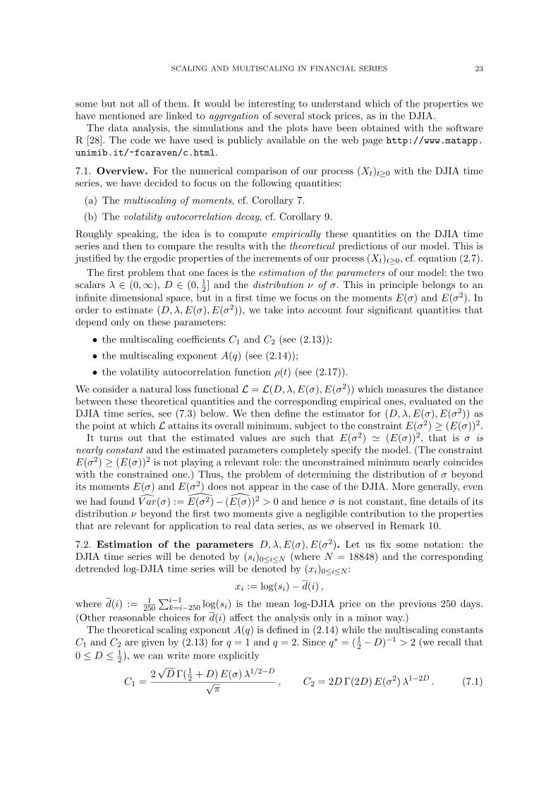