RELIABILITY OF ELECTRIC GENERATIONWITH TRANSMISSION CONSTRAINTS

by

EUGENE GORDON PRESTON

An Edited Version Of The

DISSERTATION

Presented to the Faculty of the Graduate School of

the University of Texas at Austin

in Partial Fulfillment

of the Requirements

for the Degree of

DOCTOR OF PHILOSOPHY

THE UNIVERSITY OF TEXAS AT AUSTIN

May 1997

Acknowledgments

I would like to thank my advisors, Dr. W. Mack Grady and Dr. Martin L.

Baughman, for their support and assistance. Of special importance is the support Dr.

Grady provided in the early development of the piecewise quadratic convolution

method several years ago. Without the high accuracy provided by the PQ

convolution method, the probabilistic load flow model would not have been possible.

Recently, Dr. Baughman has been very helpful in reading the drafts and giving

advice on the theory and language in this document. I am indebted to Dr. W. C.

Duesterhoeft for his support during the development of my Master’s thesis many

years ago, and I regret not having completed this dissertation before his untimely

death. I am also grateful to the other members of my dissertation committee, Dr.

Arwin Dougal, Dr. Paul Jensen, and Dr. Alan Bovik, for their patience and support

for the many years I have taken to complete this work.

I would like to thank the City of Austin for providing the environment

necessary to make this project possible. The real world problems encountered while

planning the City’s transmission system greatly influenced my thinking. In

particular, my participation on the Electric Reliability Council of Texas Engineering

Subcommittee and the Reliability Task Force has been invaluable experience in

dealing with real world transmission and generation reliability issues. I also thank

the City of Austin for tuition reimbursements and for supporting my travel to

meetings, conferences, and short courses on power system reliability topics.

I am very thankful to my parents for their loving encouragement, to my wife

Cheryl for her continuous encouragement and faith that I would someday finish this

dissertation, to my daughters Johanna and Louisa for encouraging me to also work on

my school homework, and to Peaches for keeping a watchful eye on our home.

ii

RELIABILITY OF ELECTRIC GENERATIONWITH TRANSMISSION CONSTRAINTS

Eugene Gordon Preston, Ph.D.The University of Texas at Austin, 1997

Supervisors: W. Mack Grady, Martin L. Baughman

A new probabilistic load flow (PLF) model for calculating the reliability of

large nonequivalenced electric networks with transmission constraints is given.

Generation loss of load probability (LOLP) and expected unserved energy (EUE) is

calculated first without transmission constraints as a function of load level. Then a

two step process is used to 1) calculate the cumulative probabilistic line flows from

random generator failures and 2) perform load-generator reductions to remove line

overloads. The additional EUE and LOLP due to transmission constraints is

calculated. New piecewise-quadratic (PQ) convolution methods are used to

accurately calculate probabilistic line flows for the total set of generator failure

configurations on every transmission line (>2300»1090 for the 300 generator Texas

system) in a reasonable amount of computation time. Complete coverage of all

generator outage configurations resolves problems associated with Monte Carlo and

other enumeration methods. A new method for outaging multiple transmission lines

allows the majority of probability space of all transmission line outage events to also

be calculated in conjunction with the generation outages. A large network example is

presented in which the benefit of an additional autotransformer in a large system is

calculated. Another example using the IEEE RTS benchmarks the PLF model

against a full configuration enumeration with linear programming solution.

iii

Table of Contents

Acknowledgments

Abstract

Acronyms and Definitions

Nomenclature

Chapter 1. Introduction . . . . . . . . . . . . . . . . . . . . . 1

Chapter 2. Present State Of The Art In The Industry . . 6

Chapter 3. Mathematical Concepts . . . . . . . . . . . . . 18

Chapter 4. Solution Methodology . . . . . . . . . . . . . . . 54

Chapter 5. Generation Reliability . . . . . . . . . . . . . . . 83

Chapter 6. Load Flow Solution . . . . . . . . . . . . . . . . 94

Chapter 7. Line Distribution Factors . . . . . . . . . . . . 103

Chapter 8. Probabilistic Line Flow . . . . . . . . . . . . . . 115

Chapter 9. Line Outage Model . . . . . . . . . . . . . . . . . 122

Chapter 10. Procedure For Removing Line Overloads . . 131

Chapter 11. Large System Examples . . . . . . . . . . . . . 147

Chapter 12. Test Cases Using IEEE RTS . . . . . . . . . . . 155

Chapter 13. PLF Program Output Reports . . . . . . . . . 161

Chapter 14. Conclusions and Recommendations . . . . . 176

iv

Appendix A. Derivations . . . . . . . . . . . . . . . . . . . . . . 1791. Derivation of Equation 3.11 . . . . . . . . . . . . . . . . . . . . 179

2. Derivation of Equation 3.13 . . . . . . . . . . . . . . . . . . . . 181

3. Derivation of Equation 3.14 . . . . . . . . . . . . . . . . . . . . 183

Appendix B. FORTRAN Subroutines . . . . . . . . . . . . . 1851. Sparse Matrix Solver . . . . . . . . . . . . . . . . . . . . . . . 185

2. PQ Convolution Routine . . . . . . . . . . . . . . . . . . . . . 189

3. PQ Evaluate F(x) . . . . . . . . . . . . . . . . . . . . . . . . . 191

4. PQ EUE Routine . . . . . . . . . . . . . . . . . . . . . . . . . 192

Appendix C. NERC GADS Definitions (omitted)

Appendix D. IEEE Reliability Test System (omitted)

Bibliography . . . . . . . . . . . . . . . . . . . . . . . . . . . . . . 193

Vita . . . . . . . . . . . . . . . . . . . . . . . . . . . . . . . . . . . 203

v

Acronyms and Definitions

autotransformer a transformer in which the voltage on one side can be heldconstant by varying the transformer turns ratio

BEPC Brazos Electric Power Cooperative

bus a node in the network, usually associated with a substation

CADPAD a Westinghouse distribution system analysis program

COA City of Austin, see also EUD

COB City of Brownsville

configuration the status of all lines and generators taken collectively as acollection of the on, off, and derated states of each individually

convolution a process for calculating a distribution of the probability of allpossible outcomes from random and independent events

CPL Central Power and Light

CPS City Public Service

COMREL a 200 bus composite generation-transmission program

control area a set of buses and lines within the network in which a singleowner specifies load, generation, and other requirements

CREAM medium scale 500 bus composite reliability multi-areaevaluation program based on the Monte Carlo method

decreasing an Hj,k that reduces line j flows and does not increase xmax

DFOR Derated MW generator Forced Outage Rate

DOE US Government Department of Energy

dominant the largest of the sum of line incremental flows, either + or -

EFOR Equivalent Forced Outage Rate (for 2 states) - see GADS def.

ELDC Equivalent Load Duration Curve

ENPRO a Monte Carlo production costing program with limitedtransmission constraints capability

EPRI Electric Power Research Institute

vi

ERCOT Electric Reliability Council of Texas

EUD City of Austin Electric Utility Department

EUE Expected Unserved Energy in MWh, the load shedding energy

FOR Forced Outage Rate - see GADS for definitions

GADS Generation Availability Data System published by NERC

GATOR Florida Power Corporation’s composite reliability program

GENH probabilistic Monte Carlo generation planning program usedby the City of Austin in the 1980’s

GRI Generator Reliability Indicators: FOR, EFOR, etc.

GRIP composite multi-area generation reliability program withnon-looped areas radial from a single central area

G-T generation and transmission

H a random access binary file storing array Hi,k numbers

HT the transpose of file H

increasing an Hj,k that causes an increase in line j value of xmax

LCRA Lower Colorado River Authority

LLS Loss of Load Sharing (proportionately at all load buses)

load flow an electric power system mathematical solution technique

LOL Loss Of Load in megawatts

LOLP Loss Of Load Probability = FG(x)

LP Linear Program, an optimum solution to a set of constraints

LST Load Shedding Table (optimum generation-load pairs)

MAPS a multi-area simulation program by General Electric

MAREL a multi-area simulation program by Power Technologies, Inc.

Markov a process for calculating probabilities of discrete states

MEC Medina Electric Cooperative

vii

MaxGen the unique configuration of all generators in service runningat full output; the maximum load+losses that can be served

MONA Mixture Of Normals Approximation

MWh megawatthours; used as an EUE measure

NARP N Area Reliability Program used by ERCOT

NERC North American Electric Reliability Council

NLLS No Loss of Load Sharing (load shedding assigned explicitly)

OPF Optimum Power Flow, an optimizing load flow technique

PL Piecewise Linear, a linear interpolation technique

PLF Probabilistic Load Flow, the method presented in this thesis

PQ Piecewise Quadratic, a quadratic interpolation technique

PTI Power Technologies Incorporated

PROMOD a production costing program based on convolution techniques

PSSE deterministic load flow program by Power Technologies, Inc.

p.u. per unit

RAM random access memory (a computer’s main memory in Mb)

recursive each distribution is built on a preceding distribution

REI Radial Equivalent Independent equivalent network model

reliability a measure of generation and transmission adequacy forsupplying electric power

RTS IEEE Reliability Test System, a small network for testing

R/X ratio refers to the magnitude of the line resistance to reactance ratio

single area generation reliability assessment with no transmission model

slack generation power adjusted to meet area power requirements

state a line or generator in an on, off, or derated status

STEC South Texas Electric Cooperative

STP South Texas Project

swing generation power adjusted to meet total system requirements

viii

substation a point at which one or more transmission lines terminate

SYREL a small network model predecessor of TRELSS

tail far right end of a decreasing cumulative distribution function

tie line a transmission line connecting two control areas

TMPA Texas Municipal Power Authority

TRELSS newest EPRI transmission reliability program

TU Texas Utilities

UCS Utility Consulting Service, performs studies for ERCOT

virtual generator power injected into a bus to cancel load on that bus

virtual generation a set of virtual generators to cancel (shed) load in an area

WSCC Western Systems Coordinating Council

WTU West Texas Utilities

zipflow a fast approximation method for outaging transmission lines

ix

Nomenclature

~ approximately

» approximately equal to

" x = 0, xmax , h for all x from 0 to xmax incrementing in h MW steps

li , mi outage rate (frequency) and repair rate of component i

Bi shunt reactance at bus i in per unit ohms

Ck , FORk , EFORk generator k unit MW rating, Equiv. Forced Outage Rate - p.u.

Dk , DFORk generator k MW derating, Derating Forced Outage Rate - p.u.

EUE(x) Expected Unserved Energy in MWH for one hour = òFG(x)

FA(x) generation availability distribution function

FE(x) ‘Exact’ discrete generation cumulative distribution function

FG(x) PQ generation outage cumulative distribution function

F±j(x) PQ cumulative flow distributions for line j (two directions)

F(x,y) 2D cumulative line-generation distribution function

Fp(x,y) 2D line-generation probability partial density function

Gk generator k discrete C, FOR, EFOR, and D, DFOR states

G1+...+GNg indicates convolution of discrete states, k = 1...Ng

Gk·FG indicates PQ convolution of generator k’s states into FG(x)

[Gk·FG]k=1, Ng indicates PQ convolution of all Gk states for k=1...Ng

h MW grid increment spacing for FG(x) PQ and PL functions

hj MW grid increment spacing for F±j(x) PQ line distributions

Hi,k real per unit line distribution for line i and generator k

I and I* a complex current and its conjugate in per unit amperes

Iij complex current in line i for ±1 amp injection on line j

Ibj base case line j complex current to be interrupted

[I ]b vector of n base case complex currents to be interrupted

x

[I ] n×n matrix of complex line I’s from [V ]i=1, n for n injections

INT(x) next lowest integer value of real number x

[J ] Jacobian real matrix used in load flow solution

MWO megawatts outaged

no number of lines simultaneously outaged

Na number of load areas

Nb number of load flow buses (electrical nodes in the matrix)

Ng number of generators

Nt number of transmission lines and transformers

p either a state probability or an initialization probability

Pr [X > x] probability random variable X is > real number x

DPi load flow bus i real power mismatch (+ is into bus)

[DP] load flow vector of bus real power mismatches

DQi load flow bus i reactive power mismatch (+ is into bus)

[DQ] load flow vector of bus reactive power mismatches

Rj the MW rating of line j

r a real number used in PQ and PL interpolation

sn area n load+loss MW / total generation MW

Sj complex scalar line j injection current in per unit amps

[S ] vector of n complex injection currents in per unit amps

[T ] a temporary array of numbers

V a complex number bus voltage in per unit volts (~1.00)

[V ]b load flow base case complex bus voltages of the network

[V ]j network complex bus voltages from ±1 amp injection on line j

DVi bus i temporary single precision complex incremental voltage

[DV ] vector of temporary single precision complex incr. voltages

VAi bus i double precision voltage angle as a complex number

VMi bus i real voltage magnitude; double precision in new matrix

xi

[DVM] vector of real incremental voltage magnitudes

[VM] vector of real number bus voltage magnitudes

DVMi bus i real incremental voltage magnitude

VFi bus i real voltage angle

DVFi bus i real incremental voltage angle

[DVF] vector of real incremental voltage angles

Vf j ‘from’ complex bus voltage for ±1 amp injection

Vt j ‘to’ complex bus voltage for ±1 amp injection

Vf b j line j ‘from’ bus base case load flow complex voltage

Vt b j line j ‘to’ bus base case load flow complex voltage

Vf i j line i ‘from’ complex bus voltage for ±1 amp injection on line

j

Vt i j line i ‘to’ complex bus voltage for ±1 amp injection on line jcj random variable on cj , line j probability-MW flows

xmax the maximum value of MW that will occur on real x

xoj the MaxGen (base case) line j MW real power flow

[Y ] complex admittance matrix of the total network less shunts

[Ys] complex admittance matrix of the total network with shunts

Yj complex in-line admittance of line j to be removed

xii

Chapter 1Introduction

BackgroundLarge interconnected electric power systems are carefully planned to provide

very reliable electric service. Random outages of generators and transmission lines

are normal events, and wide area blackouts are not expected to occur due to these

random outages. Therefore, the simple line outages resulting in the recurring

cascading blackouts recently in the western United States (WSCC region) were

neither planned nor expected. These blackouts are an example of unacceptable

reliability of a large interconnected system as reported by the DOE [100].

The blackouts in the WSCC were due partially to a lack of sufficient

computational tools to analyze the many possible configurations that a large system

may encounter. The planning engineers of the WSCC stated that they had never

simulated or modeled the specific conditions that led to the recent blackouts of that

system. A large system requires the testing of an immense number of configurations.

Many of these failure configurations will lead to significant loss of load, but they are

never discovered and tested because far too many configurations exist to explicitly

test all of them.

A specific example illustrates this point. Recently a study was run on a large

system in the southeastern United States [6]. An exhaustive analysis of this system

for all possible line and generator outage states would require an extremely large

number of configurations to be examined. Because the complete enumeration of such

a large number of configurations is impossible to perform, two approaches are used

today to solve the composite generation-transmission system reliability problem [7].

The two approaches are analytical enumeration and Monte Carlo simulation. Each of

these approaches takes a representative sample of the total problem with the objective

of arriving at a solution close to the totally exhaustive solution of all possible

1

configurations. In [6], analytical enumeration was used to simulate over 2.5 million

configurations. A computer run time of ~60 hours for this example was the

overriding solution constraint. To keep the computer run time reasonable, the

authors limited the problem to be studied to no more than two generators outaged at a

time.

The system in [6] has 570 generators. Assuming an extremely low generator

forced outage rate (FOR) of only 2% results in about 11 generators in a failure state

on the average. The assumption of two generators out of service is not realistic.

Furthermore, the total probability space of all combinations of two generators out of

service from a total of 570 generators is only .0008 (using an FOR of .02)1.

Limiting this study to two generators out of service misses 99.9% of the

problem to be studied! The majority of generation outage configurations causing line

overloads in the network have not been tested. The approach taken in [6] is useful

for operational planning purposes in which the states of generators out of service are

known in advance and put into the model. Beyond one or two weeks into the future,

the status of generators is not known, and the study results in [6] are incomplete.

Operating experience shows that many large scale system disturbances are

associated with clusters of generators in a configuration causing large power shifts.

These power shifts change line flows throughout the network, causing lines to

overload within the interiors of the load areas. Some models [5,26,31,62,87]

incorrectly assume that only the tie lines are the limiting transmission constraints.

The probability of any one set of generators being out of service is small.

Collectively, the total probability of all of them is significant. The approach taken in

the probabilistic load flow (PLF) model presented in this dissertation allows all of the

transmission lines in a large network to be tested for probabilistic overload for all of

the configurations of generators being out of service or derated. The PLF model

1 .98570 +570´.02´.98569 +.5´570´569´.022´.98568 = .0008 of the total probability failure space

2

presented in this dissertation also includes an efficient means for outaging any

number of one or more lines concurrently with all the generators being outaged.

Dissertation Objectives And AchievementsThe purpose of this dissertation is to present a new probabilistic load flow

(PLF) approach to solving the composite generation-transmission reliability problem

for large interconnected electric power systems (300 generators, 5000 buses). The

total set of all combinations of all generators outaged is calculated along with the

probabilistic line flows (due to the outages) using a new recursive1 convolution

technique. A new efficient line outaging technique allows the statistically significant

transmission line outage configurations to also be modeled. To accomplish this, new

methods not previously appearing in the literature are used.

1. A new convolution of line flow states method is presented in Chapter 8 in which

all combinations of random generator outage possibilities are modeled. The

new approach allows the total probability space of all independent generation

outage states to be modeled and mapped to the transmission system as

probabilistic incremental line flow states in the form of cumulative

distributions [1]. Since the coverage of all generation outage configurations is

exhaustive (complete), a fundamental deficiency of methods relying on

enumeration and sampling is solved [3]. The current industry approach to the

determination of probabilistic line flow states based on enumeration

techniques is easily shown to result in incomplete solutions (Chapters 1 and 2)

because of the enormous number of significant generation outage

configurations.

1 Cumulative probability distributions are updated as each random generator is added to the network.

3

2. A new mathematical convolution method based on piecewise-quadratic (PQ)

functions is presented in Chapter 3. The PQ mathematical convolution error

is user controllable and can be kept at sufficiently low levels to provide

accurate probabilistic line flows in Chapter 8. The new PQ convolution

methods in [1,34] have lower error than other methods such as piecewise-

linear [48], cumulants [47], and Mixture of Normals Approximation [44]

based on tests performed in [34]. The line overload problem in this

dissertation requires the right hand tails1 of the cumulative distribution

functions to have low computational error. Characteristic functions such as

MONA, Fourier Series, and Cumulants produce too much error in their right

hand tails to be applicable to this problem.

3. A new mathematical method of modeling load shedding through the use of

‘virtual’ generators at load buses is presented in Chapters 7 - 10. The virtual

generation is a means of selective load shedding within the network. Linear

combinations of distribution factors using superposition of both real and

virtual generators allow a large number of combinations of generators and

load buses to be tested for optimal load shedding.

4. A new computationally efficient method for outaging many transmission lines

simultaneously is presented in Chapter 9 and in [55]. Computation speed is

orders of magnitude faster than direct load flow enumeration. This line

outage model is an integral part of the composite generation-transmission

outage configuration model.

1 The line flow cumulative distributions in this dissertation are monotone decreasing and measure the probability of a transmission line being loaded greater than x MW. Most line overloads occur to the far right in this function in what is referred to as the tail of the function (ref. Figure 4.3 on page 74).

4

5. A new load flow solution technique is presented in Chapter 6 using two solution

matrices simultaneously in place of a Jacobian matrix. A new form of bus

voltage representation is used that allows polar to rectangular operations

without the need for trigonometric functions.

6. The total PLF solution approach presented here using all of the above innovations

together as an integrated package is new. The new approach models a greater

number of outage configurations for a much larger network (5000 buses) than is

presently possible with enumeration methods. The new solution procedure

requires a series of steps (Chapters 4 and 10) necessary to solve the composite

generation-transmission problem. In summary, these steps are: 1) set up a

maximum load and generation load flow; 2) outage each generator and calculate

all incremental line flows; 3) convolve the incremental line flow states to produce

probabilistic line flow distributions; and 4) perform load and generation

reductions to remove line overloads. Load shedding statistics are recorded and

presented as a report.

The new PLF network reliability analysis solution presented here models all

the combinations of generation outage states and the majority of significant line

outage states. A real power model is used to calculate the combinatorial transmission

line flows rather than an explicit electrical model. The use of linear line factors and

convolution techniques provides a means for achieving the most complete

computational coverage of the probability space of generator and line outages in the

industry when compared with other models presently in use.

5

Chapter 2

Present State Of The Art In The Industry

The 1965 blackout of New York City made the United States citizens and

government aware of our reliance on electricity and the unpleasant consequences of

an extended outage. Shortly after that blackout, regional councils were formed to

insure a high level of reliability is maintained. Recent actions are opening up electric

systems to competition, and reliability is one of the top three technological concerns

of the electric power industry, according to a recent IEEE Power Engineering Society

survey [4]. The Western Systems Coordinating Council recent blackouts indicate the

need to develop new tools to better measure power system reliability.

This dissertation is an advancement in the analysis and measurement of the

reliability of large interconnected electric power systems as shown in Figure 2.2. A

review of the tools presently used by the electric utility industry to measure the

reliability of large electric power systems is discussed. The following presentation is

a light discussion of the author’s personal experiences and comments on the computer

programs presently available for calculating electric power system reliability.

Personal ExperiencesIn the early 1970’s I met with Dr. A. D. Patton of Texas A&M University to

discuss new computational simulation methods for electric power systems. At that

time large system transmission planning was a deterministic process. I wanted a

better way to measure the reliability benefits associated with future transmission lines

and generators being studied. Dr. Patton said a probabilistic model could solve this

problem. His most recent publication [53] at that time modeled generation but not

transmission reliability. Large network probabilistic analysis software was not

available, although papers were beginning to appear [48-54] and [92,93]. Multi-area 6

generation models were also being discussed [31]. The simplified multi-area models

did not have the level of transmission system detail I was seeking.

Several years pass in which deterministic models dominated the planning

processes at the City of Austin Electric Utility Department (EUD). In the late 1970’s

a consultant used a new probabilistic production costing model based on Booth’s new

method [48,54] to assess Austin’s generation options. The consultant proudly

pointed out the strengths of their model and the deficiencies of the deterministic

model I was using. Not to be outdone, the EUD’s in-house production costing model

was rewritten using optimum unit commitment, optimum incremental hourly

dispatch, and Monte Carlo methods to model generator failure states. This program

called GENH was better than the consultant’s, and we learned a lot about the Austin

system with GENH. However, GENH had no provisions for modeling transmission

system constraints or line outages.

In 1985 I had an opportunity to specify and purchase the best computer

hardware and software available for generation, transmission, and distribution

planning. Hundreds of thousands of dollars were spent to insure we had the best

tools the industry had to offer (PROMOD, PSSE, CADPAD). Even after all this

hardware and software was installed and running, I still could not answer the original

question I had asked Dr. Patton a decade earlier.

In the late 1980’s the Electric Reliability Council of Texas (ERCOT) became

interested in studying the effects of transmission constraints on the reliability of

generation supply. A single area1 Utility Consulting Service (UCS) model was used2

to evaluate the reliability of generation in ERCOT. Several candidate programs were

reviewed for use in modeling transmission constraints in ERCOT. Programs under

consideration plus others that appeared later include: AREP, CONFTRA, COMREL,

CREAM, ENPRO, GATOR, GRIP, MAREL, MAPS, MARS, MECORE, MEXICO,

1 Single area means no transmission system is modeled.2 The single area UCS model is still in use as an ERCOT measure of generation reliability.

7

MULTISYM, NARP, PROCOSE, PROMOD (multi area), RECS, SICRET, SYREL,

TRELSS, and others. None of these model the total probability space of generation

and transmission failure states.

Dr. Patton’s GRIP program was reviewed first. It has a transmission link

model resembling the spokes of a wagon wheel. The one area under study is the hub

or center of the wheel, and the other utilities are at the end of the radial spokes. The

spokes are transmission links that are assigned capacity and availability states.

ERCOT considered using the GRIP program and decided not to use it because the

ERCOT system resembles enclosed loops rather than radial spokes. One large

ERCOT utility uses the GRIP program to study its own service area reliability, which

is the center hub utility, and radial ties are made to the other major control areas.

This arrangement gives no information about transmission limitations within the

remote areas outside the hub or within the hub area itself. It does allow power import

constraints to be specified.

Another program called MAREL by Power Technologies, Inc. uses a more

general radial model than GRIP in which radial links can be taken off any node in the

network. However, MAREL has the same limitation as GRIP in that it does not

model loops or loop flows. ERCOT felt strongly that modeling loop flows is a

necessity. Dr. Patton proposed a three area loop model, but it was also believed to be

too simplistic.

To overcome these shortcomings, Drs. Patton and Singh were hired by

ERCOT to develop a new program called NARP [5,62]. The NARP network model

for ERCOT is an 8 node 13 link model of the ERCOT transmission system as shown

8

in Figure 2.1. Each node is a major load area such as Austin, Houston, Dallas, San

Antonio, etc. and each node contains the generators physically local to that area

(node). Network flows are calculated using a DC load flow which can model loops.

Monte Carlo is used to randomly outage generators. A linear program optimally

performs load shedding when link overloads occur. The links can be assigned

capacity and probability states. The NARP program is easy to run, but the original

link model shown in Figure 2.1 was difficult to develop and calibrate.

WTU TU

COA LCRA TMPA

BEPC

CPS HLP

STP

CPL COB

STEC-MEC

Figure 2.1 The NARP Network Model For ERCOT

No software was delivered with the NARP program to create the NARP 13

transmission link elements shown in Figure 2.1. The link model had to be manually

‘tuned’ to get the best agreement with full AC1 network load flow on incremental tie

flows between areas. This tuning effort was difficult and time consuming and has not

1 AC means complex circuit impedances, line currents, and line powers are modeled.

9

been repeated since the initial equivalent was developed. In spite of these limitations,

the NARP program was and still is a state of the art program in its ability to impose

transmission limitations on the reliability of the generation supply. A more detailed

transmission link model for NARP using what is called an REI model has recently

been published [62], but this model has not been used to perform ERCOT studies.

When the NARP program was put into use to study the ERCOT system, an

undesirable characteristic of Monte Carlo was discovered. If the ERCOT generation

capacity is increased to 30% above annual peak ERCOT load, the NARP program

has difficulty finding failure configurations using the Monte Carlo random draws to

determine outaged generators. Some NARP runs required a week of execution time

on a 486DX 50 MHz PC to find only 100 events with loss of load. A week of

computer execution time for the ERCOT system in Figure 2.1 is typically 100,000

repeat simulations on a single year in which each day is tested for the peak daily load

condition. These very long computer run times prevent a meaningful study from

being performed because only a few questions can be studied and answered. I

learned from this experience and my earlier experience with the GENH production

costing program that Monte Carlo is better suited to production costing than

reliability analysis. In general, the Monte Carlo method increases in computer run

time and decreases in accuracy in proportion to generation reliability. This means

that an engineer performing a study in which the system is made increasingly more

reliable will experience longer and longer computer run times. In contrast to this

problem, the convolution method used by the PLF model improves in accuracy as the

system is made more reliable and the solution run time decreases. The very long run

times required for Monte Carlo effectively cripple the NARP program in the final

stages of a study. Completing a reliability study in a reasonable amount of time using

the Monte Carlo method may be very difficult.

10

Capability Of Presently Available Computer ProgramsFigure 2.2 shows how the PLF model by Preston, Baughman, and Grady in

[1] compares with other models concerning the level of detail in modeling both

generation and transmission systems as an integrated system.

none a few selected Monte Carlo all configurationsGeneration Detail

Figure 2.2 Transmission Detail Versus Generation Detail

Figure 2.2 shows a tradeoff between program complexity in generation and

transmission representation of detail both electrically and probabilistically. Programs

with very detailed probabilistic transmission analysis are usually incomplete in the

treatment of random generator outages (TRELSS). The opposite is also true.

Programs that have a complete treatment of the random outage of generators have a

highly reduced transmission network (MAREL). In all these programs the computer

run time is long. Compromises are made to keep computer execution times

reasonable. This section discusses the compromises that have been made in the

design of these programs.

TRELSS not yet achievedPSSE

RECSCREAM

SYREL complexCOMREL

simpleNARP MARELENPRO GRIP

trivial PROMOD

GENH

11

PLF

Discussion:

Probabilistic programs with detailed transmission representation [6,24] are

RECS, SYREL, CREAM, and TRELSS. These programs explicitly enumerate

selected configurations of randomly outaged lines and generators. An OPF and/or an

LP is used to take corrective actions to minimize the loss of load. Configurations to

be enumerated are selected based on a screening process of probability and likelihood

of having a transmission constraint. The earlier EPRI transmission reliability

evaluation program called SYREL is a 150 bus network model. EPRI replaced it

with the TRELSS program [24] which has a network capability of approximately

2000 buses. In [6] an example is given in which a 2182 bus, 3791 line, 8 area, 570

generator system required ~60 hours of execution time to enumerate 2,534,336

failure configurations of any two generators and/or lines out of service

simultaneously. This example illustrates how the computer run time is a limiting

factor in how deep the contingencies are allowed to proceed in a TRELSS run. The

total number of configurations for this problem exceeds 2(570+3791)»101300. On top of

this number of generation and line outage configurations, each overloaded line has a

unique set of generator outage and line outage configurations causing the line

overloads. Enumeration sampling will not be able to cover this space adequately.

Even with 62 hours of computer run time, [6] did not adequately measure the

reliability of that system since only two levels of generators were outaged.

The CREAM program [17] is similar to TRELSS but uses Monte Carlo to

select line and generator configurations rather than enumeration. It has a smaller

network of 500 buses maximum, which is too small to model the full ERCOT

system. There is no simple way in the CREAM program to create a reduced ERCOT

transmission model and retain all the electrical characteristics of the full network.

The CREAM and TRELSS programs have not been implemented and tested for

ERCOT, although individual utilities in ERCOT have tested these models.

12

The ERCOT experience with NARP indicates that many generators must be

outaged simultaneously to create loss of load conditions to measure both the

reliability of generation and to encounter transmission constraints in the small NARP

equivalent transmission model1. If this is true, then the TRELSS program is skipping

over a significant amount of the generation outage events that cause load shedding.

Probabilistic programs with exhaustive modeling of generation outage states

and limited transmission models are MAREL, GRIP, and PROMOD. PROMOD is

not designed to calculate reliability, but it does model all generation failure

configurations using the Booth-Baleriaux method [48]. The GRIP program partitions

annual load into weekly ELDC sets and uses Booth-Baleriaux, or mathematics similar

to Booth- Baleriaux, to perform the convolution of generation states. The GRIP

multi-area transmission model resembles a wagon wheel in which one central area

under study is surrounded by other areas connected radially to the central area. Each

area has generators that fail randomly.

The NARP program uses a transmission equivalent model that treats all the

parallel lines connecting adjacent areas as a single lumped equivalent. Figure 2.1

shows the NARP equivalent link model developed for ERCOT. Each area is a node.

Nodes are connected by single lumped equivalent lines. The power flow on each line

in the NARP equivalent is determined by a DC load flow. Overloaded lines are

unloaded by optimal load shedding using an LP. This simple model has intuitive

appeal, as evidenced by the number of papers using this model [3,5,25,26,62].

However, no papers have been published showing a procedure for calculating a

reduced network’s set of impedances, capacities, and probability states.

The REI equivalent method is presented in [62] as an advanced reduced

network model with the details of constructing the REI equivalent given in [87].

Figure 2.3 shows the connectivity of the REI between power plants and interarea tie

1 NARP results show ERCOT transmission loss of load expectation highest for approximately 10 to 20 generators simultaneously in failure states for the ~300 ERCOT generators.

13

lines. However, the REI in [87] is a deterministic equivalent. There is no provision

for handling line outages and their effect on system reliability. The REI model in

[62] presumes that monitoring tie lines between areas is sufficient to capture

transmission constraints. Actual ERCOT load flow studies show that this is almost

never the case. Usually the limiting lines are internal to each system, and these

internal lines restrict generation.

Area 1 Power Plants Area 2 Power Plants

REI Equivalents Tie Lines

Figure 2.3 REI Tie and Equivalent Lines Between Two Areas

A problem with equivalent networks is their inability to explicitly model real

transmission line failures. The REI model must be completely rebuilt for each

transmission line(s) outaged in the real network. In [62] there was never any

intention of using a different equivalent for each full AC network transmission outage

configuration. The thought in [62] is to give the tie lines a set of availability states

and capacities to represent the full AC network’s transmission constraints.

Unfortunately, the theory to do this has not been developed. The literature is

completely lacking on the theory needed to develop a composite generation-

transmission probabilistic equivalent network. This explains why the group of

ERCOT engineers had to struggle in their effort to construct an equivalent network

model for the NARP program. The theory was weak in this area, and this caused

them to waste time using simple manual adjustments to get better agreement between

14

the full AC load flow and the equivalent. The author spent a great amount of

personal time testing and tuning this model. The REI was proposed by Dr. Patton as

an improved network model but was never implemented. Whether the REI model

would have been easy to create and produce useful results is unknown.

NARP uses the Monte Carlo sampling technique which has an improvement

in solution accuracy proportional to N where N is the number of simulations. In

[17] the authors illustrate this slow improvement in accuracy by stating “...a system

LOLP of .001 with an uncertainty of 30% would require ten thousand samplings; the

reduction of this uncertainty to 3% would require a sample size of one million.”

Gaining one more digit accuracy requires a hundredfold increase in execution time.

Research on improving the rate of convergence for Monte Carlo continues, and an

example of this is described in [18].

The PSSE program in Figure 2.2 refers to the original PTI load flow

programs purchased by the EUD in 1985. They have a high level of detail in the

transmission models including transient stability and OPF. The original PSSE

programs have been deterministic models for years. Possibly PTI held off

development of a probabilistic load flow because they already had a composite G-T

program in MAREL. The recent introduction of the General Electric MAPS program

and the EPRI TRELSS program may have changed PTI’s thinking on probabilistic

load flow. Recently PTI has offered a two area probabilistic load flow based on

enumeration of line outages, and another new probabilistic load flow has recently

been introduced.

The ENPRO program was purchased by the EUD to perform detailed

chronological production costing. ENPRO uses the Monte Carlo method. It has a

limited transmission model in which a few lines can be monitored for overload.

ENPRO is similar to PROMOD in not being able to model generation reliability.

The Booth-Baleriaux method Dr. Booth of Australia developed [48,49,54]

works very well in commercially available production costing programs (PROMOD). 15

Booth-Baleriaux used in production costing is usually applied to just one load area

under study. This solution does not measure generation reliability at all. Without the

total set of generators in a study, the information on the improvement in reliability

from the interconnections [13] is not calculated. To correct this deficiency in the

EUD studies, a multi-area version of the PROMOD program was purchased by the

EUD with the thought of using this one program to measure overall reliability of

generation supply as well as perform production costing. This effort failed when it

was discovered that the multi-area model used expected (average) tie line flows

rather than distributions. The tie flows between areas were identified as being

approximations to the actual set of probabilistic flows. The specific configurations of

generation and load that would have caused tie flow overloads were not calculated in

this approach. The use of the multi-area PROMOD program to measure the City of

Austin generation reliability was dropped.

Other analytical probabilistic methods [35,38,40-44,47] not shown in Figure

2.2 have been developed for use in production costing programs. These execute very

quickly but have a rather large amount of error in the tails of the probabilistic

distribution functions where the reliability information is contained. Some methods

such as Fourier [40] and cumulants [41-43,46,47] can produce negative probabilities

in the tails of the distributions. The cumulant method is very fast and is used in

production costing programs in which the expected value of the function is in the

range of interest [35-47] for calculating average energies of each generator.

However, the reliability information is in the distribution function’s tails where the

function has extremely small values just barely greater than zero. In this region there

can be much relative error. Any functional ringing will introduce extremely high

error in the calculation of reliability. The large error in this region when using

cumulants has led to a widespread belief that production costing programs are not

capable of calculating reliability, since most of them use a fast convolution scheme

such as cumulants.

16

The Booth-Baleriaux method can have good accuracy in both production

costing and reliability, as shown by Preston and Grady in [34], however, it may be a

little slower to execute than the analytical methods. In this dissertation, the Booth-

Baleriaux model is improved using the PQ convolution procedure. The PQ

convolution method is extended to include the calculation of probabilistic line flow

distributions. Although PQ does not appear to the fastest solution approach, when

overall accuracy is taken into account, the author believes it is the fastest in the

industry. The fact that PLF can model large systems in reasonable computation times

is evidence supporting this belief.

17

Chapter 3Mathematical Concepts

The composite generation-transmission analysis problem requires the

generation outage configurations be examined more completely than enumeration

methods are capable of providing. A convolution of states approach, using a

recursive technique1, is preferred because it allows for coverage of the entire

probability space of all generation outage events. This approach, which is widely

used in modeling probabilistic generation outages in [35,38,40-44,47], is extended in

this dissertation to include the transmission system.

The mathematical theory presented in this chapter starts with basic concepts

and ends with a presentation of the piecewise quadratic (PQ) convolution method.

Papoulis [98] and Stark [99] suggest the user avoid a direct convolution process (like

PQ) because it is considered by them as computationally intensive (too slow). Their

recommendation is to transform the problem into a form in which the convolution is

simplified such as Fourier series [40] or cumulants [41-43,46,47]. Mixture of

normals approximation [34,38,44] is another popular approach. However, experience

shows these methods produce too much error in the tails of the probability

distributions of the line flows. The PQ convolution method in this dissertation allows

the convolution process to be performed with a high degree of accuracy for hundreds

of generators whose output power states are random variables. The piecewise linear

(PL) method [34,48,49,54] is presented as an introduction to PQ because of its

simplicity and similarity to the PQ method, although the PL method also is found to

have too much solution error to be used for calculating line flows.

Basic Concepts1 Recursive means each distribution is built on the preceding distribution rather than by binomial theorem expansions and the subsequent merging of tables of data [52].

18

Electric generators are complex machines that typically have a probability of

being in a state of failure of 5% to 10%. When they do operate, their maximum

output capacity is a variable depending on ambient temperature, fuel heat content,

amount of excess air used, air and water environmental constraints, and other

operating conditions. The exact maximum capacity of each generator is uncertain.

Most power plants have internal redundancy of components that wear out or fail

frequently. The mill for grinding coal to a powder is an example. A generator may

have several mills and a standby. When one fails, the maximum capacity of the plant

may be reduced. This type of outage happens often enough to create a cluster of

capacity states around a derated output MW level for the coal plant. Figure 3.1

shows what the distribution density of capacity states f(x) might look like for a

typical generator. The maximum capacity (C) has uncertainty. The clustering of

points around one or more frequently occurring derated (D) states is also shown.

Since a generator will be taken completely off line for very severe problems, a gap

between the operational states and the outage state is created, as shown in Figure 3.1.

The probability of running a severely damaged generator at very low MW levels is 0.

f(x)

out of service operating

x MW

0 D C

Figure 3.1 Maximum Output Capacity of a Generator as a Random Variable

An example is given to show how the distribution of capacity states of two

generators with continuous distributions of densities can be convolved together to

form a new function of the total probability of generation capacity being available.

19

Figure 3.2 and Equations 3.1 and 3.2 show generator 1 with a uniform distribution

from 0 to 1 MW. Generator 2 has an exponential distribution from 0 to 1 MW. The

capacities of the two generators are assumed to be independent, which is required to

perform the convolution process shown in this example.

f1(x1) f2(x2)

x1 MW x2 MW 0 1 0 1

Figure 3.2 Probability Density Functions For Two Generator Example Problem

The figures above are described by

f1(x1) = u(x1) - u(x1-1) (3.1)

and

f2(x2) = ex2(e-1)-1[u(x2) - u(x2-1)] (3.2)

where u(x) is a unit step at x = 0.

Let x = x1 + x2. The convolution of generation states is performed in Equation 3.3

and successive steps as

ó ¥ ó x-x2

(f1·f2)(x) = ô ô f1(x1)f2(x2)dx1 dx2, (3.3)õ-¥ õ-¥

20

then

ó ¥ ó x-x2

(f1·f2)(x) = ô ô [u(x1)-u(x1-1)] × [ex2(e-1)-1{u(x2)-u(x2-1)}] dx1 dx2 ,õ-¥ õ-¥

andó ¥

(f1·f2)(x) = ô ex2(e-1)-1× [u(x2)-u(x2-1)] × [u(x-x2)-u(x-x2-1)] × (x-x2) dx2 .õ-¥

The functions being integrated are discontinuous, which creates two

overlapping regions as shown in Figure 3.3.

x-1 0 x 1 0 x-1 1 x

Figure 3.3 Convolution Intervals For Two Generator Example

These regions are integrated as two separate integrals as shown in (3.4).

ó x

(f1·f2)(x) = ô ex2(e-1)-1 × (x-x2) dx2 for 0 £ x £ 1õ0

ó 1

ô ex2(e-1)-1 × (x-x2) dx2 for 1 £ x £ 2 (3.4)õx-1

The final solution is

(f1·f2)(x) = (ex - 1)(e - 1)-1 for 0 £ x £ 1

(e - ex-1)(e - 1)-1 for 1 £ x £ 2 . (3.5)

21

The convolved generator states for this example are shown in Figure 3.4.

1

f(x)

00 1 2 MW

Figure 3.4 Distribution f(x) For Two Generator Example

The continuous distributions in the two generator example can be represented

as a set of discrete states as shown in Figure 3.5 and Table 3.1. This example will

show that a discrete state model can be used instead of continuous states for

calculating the cumulative probability generation capacity outaged will exceed x

MW.

f1(x1) f2(x2)

x1 MW x2 MW 0 1 0 1

Figure 3.5 Discrete Generator States For Two Generator Example Problem

Table 3.1 Generator Discrete State Values For Figure 3.5

x1 gen 1 state prob x2 gen 2 state prob

.125 .25 .125 .1653

.375 .25 .375 .2123

.625 .25 .625 .2725

.875 .25 .875 .3499

22

Each state of each generator is combined once with each of the states of the

other generator by summing x MW and multiplying probabilities. This produces 16

state probabilities. Many of these states have the same MW. The probabilities of

equal MW states are summed. Table 3.2 shows these combined state probabilities.

The combined discrete states are a convolution of the two discrete state generators.

The last two columns of Table 3.2 show the cumulative probability generation

capacity available is less than or equal to x MW for the discrete states and for the

continuous distribution shown in Figure 3.4.

Table 3.2 Discrete And Continuous Probability Generation Capacity G£ x MW

x MW discrete state prob discrete Pr[rvG£x] continu

Pr[rvG£x]

.00 .000 .000 .000

.25 .041325 .041325 .0198

.50 .0944 .135725 .08655

.75 .162525 .29825 .2136

1.00 .25 .54825 .418

1.25 .208675 .757 .6482

1.50 .1556 .9125 .8315

1.75 .087475 1.00 .9544

2.00 .000 1.00 1.000

Figure 3.6 on the next page shows the graphs of the last two columns in Table

3.2. The curves in Figure 3.6 are the discrete and continuous distributions for the

probability of total generation available being less than or equal to x MW.

23

0

0.1

0.2

0.3

0.4

0.5

0.6

0.7

0.8

0.9

1

0 0.25 0.5 0.75 1 1.25 1.5 1.75 2

MW

Pr

Figure 3.6 Discrete And Continuous Pr[generation £ x] For Two Generator Example

A more useful format is the probability generation capacity outaged exceeds x

MW. This results in a monotone decreasing function as shown in Figure 3.7 below.

Figure 3.7 is the same graph as Figure 3.6 except the x axis is reversed.

0

0.1

0.2

0.3

0.4

0.5

0.6

0.7

0.8

0.9

1

0 0.25 0.5 0.75 1 1.25 1.5 1.75 2

MW

Pr

Figure 3.7 Discrete And Continuous Pr[generation outaged > x]

24

The next example is an introduction to the idea that a transmission constraint

will cause a shift in the generation states of a generator. The four discrete states for

generator 1 in the previous example are now limited by a transmission line with a

maximum capacity of .5 MW as shown in Figure 3.8.

.5 MW max.

G1

Figure 3.8 One Generator Example With A .5 MW Transmission Constraint

This transmission constraint limits the random variable generation to a

maximum of .5 MW. The generator output power from .5 < x £ 1 MW is shifted

downward to x = .5 MW. An impulse with area of .5 appears at x = .5, as shown in

Figure 3.9 for both the continuous and discrete generator state models.

.5

.25

f(x)

0 1 MW

Figure 3.9 Distribution Of f(x) With A Transmission Constraint

This example illustrates the basic approach taken in this dissertation.

Whenever line flows exceed line capacity, generation is reduced until the overloaded

lines are no longer overloaded. Probabilistic line flows are adjusted in conjunction

with the most offending generators causing the lines to be overloaded. This reduction

in generation (and load) is identified as being caused by a transmission constraint.

25

Discrete StatesThe generators in the example just described have continuous distributions.

The industry practice is to describe individual generators with discrete states at the

cluster points C and D (shown in Figure 3.1) rather than as continuous functions.

There is a good reason for this. Generators usually operate for long periods between

major outages. The scant amount of statistical data available for individual

generators is insufficient information for developing continuous distributions. Two

state discrete generator states are the norm unless a generator clearly has derated

states that are likely to occur. A three state generator is common for this case. The

preparation of generator outage data is described in the North American Electric

Reliability Council (NERC) GADS. Appendix C gives the definitions of GADS

terms used by NERC. Table 3.3 shows the definition for the set of Gk (generator k)

success, failure, and partial failure states.

Table 3.3 Two State and Three State Definitions of Gk

Two State Model:

Probability Output Power - MW Status

1-EFORk 0 up

EFORk Ck down

Three State Model:

Probability Output Power - MW Status

1-FORk-DFORk 0 up

DFORk Ck -Dk derated

FORk Ck downIn Table 3.3, EFORk is an equivalent forced outage rate (a probability) of Ck

megawatts (being outaged) and is used only in the two state model. FORk and

26

DFORk are the three state forced outage and derated forced outage rates, respectively

(Markov state probabilities), of Ck and Dk megawatts. These states are calculated by

collecting data for the l and m (failure and repair) rates described in the next section.

Additional information on the calculations of EFOR, FOR, and DFOR is given in

Appendix C1. Note that Dk in Table 3.3 and Figure 3.14 is the MW derating, whereas

in Figure 3.1, D is shown as the derated generator output, i.e. Dk=Ck-D.

Markov ProcessAfter a generator i is outaged or is in a state of failure, there is an average

repair time Tr to put it back on line. The repair rate (number per year) is mi = Tr-1.

Likewise, a generator that has been repaired is expected to run for an average time to

failure of Tf . The rate of failures per year is li = Tf-1. Sometimes a generator will fail

to a derated or partial output power state. That case is discussed later. Figure 3.10 is

an illustration showing the two generator states of fully available and outaged.

Up P1 = Pr (unit i is available)

mi li (repair/fail transition rates)

Dn P0 = Pr (unit i is down or outaged)

Figure 3.10 Two State Generator

The failure of any given generator, transmission line, or transformer in an

interval of time 0 to t is often expressed according to Equation 3.6 in which li is the

Pr [generator i will fail] = ( 1 - e-li t ) for li>0 t³0 (3.6)

1 ERCOT represents generators ³ 500 MW with three states and < 500 MW as two states.

27

average number of failures per period. If generator i is not in a state of failure, the

probability generator i will fail increases with time in accordance with (3.6). Given

enough time, generator i will eventually fail. The exponential distribution is

discussed by Papoulis [98] and Stark [99]. Anders [36] gives several examples using

the exponential distribution, and Patton [53] presents actual electric generator data

justifying the appropriateness of the exponential distribution.

The probability of being in either the up or down state can be calculated as a

stationary stochastic discrete-valued independent random variable process known as a

Markov chain [36, 53, 98, 99]. Over a long time period, the number of transitions

into and out of each state must be conserved. This can be used to write steady state

equations for the probability of being in a specific state. For the two state generator,

the number of transitions out of the up state is equal to the number of transitions into

the up state. In equation form this is P1li = P0mi . The other requirement is for

P1+P0=1. Solving these equations for up and down probabilities P1 and P0 yields

mi liP1 = ---- and P0 = ---- . (3.7)

li+mi li+mi

If the repair rate is high and the failure rate is low, then P1 >> P0 , which is desirable

because it represents a very reliable generator.

The three state model shown in Figure 3.11 is frequently used for larger

generators with internal redundant components. These internal components are

usually designed to allow the generator to continue operation at reduced levels while

the damaged components are being repaired.

28

Up P1 = Pr (full output)

m2 l2

m1 l1 Pa P2 = Pr (partial output)

m3 l3

Dn P3 = Pr (no output)

Figure 3.11 Three State Generator

Equation 3.8 shows the Markov steady state equation for calculating the

probabilities P1, P2, and P3 of being in the up, derated, and down states, respectively,

for the failure and repair rates of the three state generator in Figure 3.11.

l1+l2 -m2 -m1 P1 0

-l2 m2+l3 -m3 P2 = 0 (3.8)

1 1 1 P3 1

A Markov steady state matrix can also be used to find the probabilities of

each of the states of many generators. Consider the three generators shown in Figure

3.12. Let each generator have a frequency of failure of one time per year (l=1).

Then let m1=9, m2=4, and m3=2.333. The generator forced outage rates are .1, .2, and

.3, respectively, when calculated using Equation 3.6 for P0 = Pr(of being outaged).

U U U29

9 1 4 1 2.33 1

D D D

unit 1 unit 2 unit 3

Figure 3.12 Three Two-State Generators In Combination Example

Eight combinations of states can be formed using these three generators. Let

UUU mean all three are up, UUD means units 1 and 2 are up and unit 3 is down, etc.

Figure 3.13 shows the eight Markov states diagram for this example.

30

P1

UUU2.33 9

4

1 1 1P2 P3 P5

UUD UDU DUU9 2.33 9 2.33

4 4

1 11 1 1 1

P4 P6 P7

UDD DUD DDU

9 4 2.33

11 1

P8

DDD

Figure 3.13 Markov State Space of Three Generators In Combination Example

From the above state space diagram, equations can be written around each

state describing a steady state flow of failures and repairs at each state or node in

Figure 3.13. The state probabilities are P1, P2, ... P8. Equation 3.9 is the Markov

equation for this three generator system. The relevance of this example is to illustrate

one of the many ways this problem can be solved. Use of the Markov process is the

first example using this three generator system.

31

3 -2.3 -4 0 -9 0 0 0 P1 0

-1 4.3 0 -4 0 -9 0 0 P2 0

-1 0 6 -2.3 0 0 -9 0 P3 0

0 -1 -1 7.3 0 0 0 -9 P4 0

-1 0 0 0 11 -2.3 -4 0 P5 0

0 -1 0 0 -1 12.3 0 -4 P6 0

0 0 -1 0 -1 0 14 -2.3 P7 0

1 1 1 1 1 1 1 1 P8 1

Equation 3.9 Markov State Space of Three Generators In Combination Example

Solving Equation 3.9 produces P1=.504, P2=.216, P3=.126, P4=.054, P5=.056,

P6=.024, P7=.014, and P8=.006. This same solution result is also obtained by other

means, as shown in Figures 3.15 (binary tree) and 3.16d (cumulative distribution).

The Markov equation approach is limited to relatively small problems. We

need to be able to readily solve problems with as many as 101000 states. Using the

Markov for this large problem would require a matrix of 101000 rows and 101000

columns, which is unlikely to ever be computationally feasible. The Markov chain

equation of discrete states is probably limited to no more than a few thousand

variables at most, which is far too few for this power system reliability problem.

The use of cumulative distributions and recursion will allow the extremely

large number of 101000 states to be calculated efficiently. The recursive process will

update the cumulative distributions as each generator is added to the system. These

curves store the probability information of all the generators convolved through the

last one convolved. This approach results in an approximately linear relationship

between computational time and the number of randomly failing generators and lines.

32

(3.9)

=

Cumulative DistributionsCumulative monotone decreasing functions (Figure 3.7) in this dissertation

are used to describe probabilistic distributions rather than the traditional monotone

increasing functions (Figure 3.6). The computational mechanics of the piecewise

quadratic (PQ) method result in low error in the far right hand tail of the cumulative

distribution for a monotone decreasing function. Distributions for extremely small

probabilities (such as 10-100) are accurately calculated. Interpolation error using the

PQ method is discussed in this chapter.

In order to have confidence that the PQ method is producing correct and

sufficiently accurate results, the PQ solutions are benchmarked with other methods

such as a binary tree solution, a Markov chain solution, and an ‘exact solution’

developed by George Gross [44]. His ‘exact solution’ is limited to systems with

generators having discrete integer real power states. The ‘exact’ distribution

FE(x) = Pr[generation outaged > x] is developed and is used to measure the

interpolation error of the PQ distribution FG(x) = Pr[generation outaged > x].

Convolution Of Generator States ProcedureThe process of recursive convolution for a generator with three discrete states

into a continuous function F(x) is a process of scaling, shifting, and summing the

F(x) = Pr[generation outaged > x] function. Figure 3.14 shows the process steps

pictorially for the three state generator in Table 3.3.

The convolution process on the function F(x) in Figure 3.14 is the sum of

three partial states. Only the derated and down states shift F(x) to the right, which

requires a linear or quadratic interpolation. The more likely to occur up state is not

shifted. It is scaled in place without interpolation, thereby reducing interpolation

error. If the up state were to be shifted, the convolution error would increase.

33

´(1-DFOR-FOR) no shift

up state

´DFOR shift of Dk MW sum

before Gk derated state after Gk

´FOR shift of Ck MW

down state

Figure 3.14 Pictorial Representation Of A 3-State Recursive Convolution Process

Development of the FE(x) DistributionA procedure is given for calculating FE(x), which is an almost exact solution

to the probability that generation power outaged is greater than x MW. Ck and Dk

must be integer values1. FE(x) is given in Equation 3.10 as

FE(x) = Pr [G1+ G2+ G3+...+ GNg (outaged MW) > x ] (3.10)

where Pr is the probability all generator Gk random outage configurations is > x MW.

1 All the ERCOT generators have integer Ck and Dk .

34

Equation 3.10 lacks the structure needed to describe how FE(x) is to be

numerically calculated in the computer. In practice, FE(x) is an array of discrete

probabilities in one MW steps starting at x=0 MW and ranging up to xmax =Ck

k

Ng

1 .

The convolution process for calculating new FE(x)+ is shown in Equation 3.11

for generator k and pictorially in Figure 3.14. The FE(x)+ replace the FE(x) after all

generator k states for all x=0...xmax have been calculated. The real whole numbers x

in a computer program are converted to integers and are used as the array index for

FE(x). Note that the grid spacing for FE(x) is 1 MW increments. When setting up the

computer program solution for FE(x), the initial values are FE(0) = 1 and FE(x>0) = 0.

Note that in Equation 3.11 any FE(x < 0) = 1.

[FE(x)+ = (1-FORk-DFORk)×FE(x)

+ DFORk×FE(x-Dk)

+ FORk×FE(x-Ck) ] " x = 0, xmax , h=1 (3.11)

Equation 3.11 is a recursive convolution process illustrated in Figure 3.14.

Appendix A.1 gives the derivation of Equation 3.11. At any intermediate point in the

convolution process, any generator not previously included in FE(x) can be added to

FE(x) using Equation 3.11. The generators can be added one at a time in any order.

The final FE(x), as a measure of total system generation reliability, contains all the

generators in the network, and is the same function regardless of the sequence or

order in which the generators are convolved1.

1 except for small numerical errors due to rounding and truncation in the computer

35

Verifying The FE(x) Solution A three generator example is used to illustrate that the FE(x) convolution

process itself produces a correct solution. Let Gk be two state generators with an

EFOR for generators 1, 2, and 3 of .1, .2, and .3, respectively. Ck generator

capacities are 100, 150, and 200 MW, respectively. For this small system, a binary

tree solution to FE(x) is constructed as shown in Figure 3.15. We have complete

confidence in the binary tree solution for this small system. This example will show

that Equation 3.11 produces the same results as a full enumeration of all explicit

configurations in the binary tree. The eight configurations possible are calculated by

adding capacities and multiplying probabilities and are then sorted and summed.

Individual States CumulativeUnit 1 Unit 2 Unit 3 MW Pr MWO MWO Pr Pr

20, .7 -- 45, .504 0 0 .504 1.000

15, .8 0, .3 -- 25, .216 20 10 .056 .496

10, .9 0, .2 20, .7 -- 30, .126 15 15 .126 .440

0, .3 -- 10, .054 35 sort 20 .216 .314

20, .7 -- 35, .056 10 25 .014 .098

0, .1 15, .8 0, .3 -- 15, .024 30 30 .024 .084

0, .2 20, .7 -- 20, .014 25 35 .054 .060

0, .3 -- 0, .006 45 45 .006 .006

Figure 3.15 Binary Tree of Three Generator Example

The last column of Figure 3.15 is FE(x)=(Pr{Gk outaged > x}) where

x = MWO, the MW outaged. The MWO is the compliment of the MW available,

which is why the last column is summed from bottom to top (see Figure 3.7).

Equation 3.11 can be used to produce FE(x) directly rather than using the

binary tree method. The advantage of using Equation 3.11 is that several hundred

36

generators can be convolved with a high degree of computational accuracy. A binary

tree solution can easily have a tree too large to be calculated. Binary tree cumulative

errors cannot be easily controlled, so the binary tree approach should be used only to

create FE(x) for a very small number of generators.

The binary tree example is given in Figure 3.15 is to verify that Equation 3.11

produces the same FE(x) results. The convolution process to create FE(x) is shown

graphically in Figure 3.16 to better illustrate the details of the process. Figure 3.16a

shows the convolution of generator 1, Figure 3.16b of generator 2, and Figure 3.16c

and Figure 3.16d of generator 3. Figure 3.16c shows the intermediate convolution

details of creating the new up states by scaling by .7 with no shift and of creating the

down states by scaling by .3 and shifting by 30 MW the immediately previous FE(x).

The two scaled curves are then added to produce the final FE(x) shown in Figure

3.16d. The process produces exactly the same solution as the binary tree method

when the states in Figure 3.16d are compared with the last column of Figure 3.15.

This process shown in Figure 3.16 is exactly the same as the process shown in Figure

3.14.

37

1.0 1.0

Pr + (10, .1) => Pr

.1 x x

0 10 20 30 40 0 10 20 30 40Figure 3.16a. Convolving G1 Into FE(x)

1.0 1.0

Pr + (15, .2) => Pr.28 .2

.1 .02 x x

0 10 20 30 40 0 10 20 30 40Figure 3.16b. Convolving G2 Into FE(x)

1.0 1.0

Pr + (20, .3) => Pr .196 .14 .3 .014 .084 .06 .006.28 .2 ´.3

.02 ´.7 x x

0 10 20 30 40 0 10 20 30 40Figure 3.16c. Convolving G3 Into FE(x)

1.0

FE(x) = Pr .496 .44 .314.098

.084 .06 .006 x

0 10 20 30 40

Figure 3.16d. Final FE(x) for Three Generator Example Using Equation 3.11FE(x) = Probability More Than x MW Of Generation Will Be Out Of Service

(probabilities are not drawn to scale)

38

Necessity For The Use Of Continuous FunctionsThe use of discrete states on 1 MW intervals for FE(x) provides nearly zero

error distributions for discrete generation capacity outaged. However, incremental

transmission line flows are never exact multiples of 1 MW. Also, the 1 MW intervals

are very computationally intensive. Greater computational efficiency is realized by

using linear and quadratic interpolation of discrete point functions. Figure 3.17

shows a piecewise linear (PL) continuous function and how interpolation error can

occur when using the PL interpolation. Error is minimized around 1000 points to

represent the PL F(x), but begins to increase if too many points are used. A bad

characteristic of the PL interpolation error is that it increases multiplicatively

(exponentially) as each new generator is added to F(x).

Pr

h MW

xmax

x : 0 1h 2h 3h 4h .... nhGeneration MW Out Of Service

Figure 3.17 Piecewise Linear Distribution Functional Representation

39

linear interpolation undershoots here

0

1

Piecewise Linear ConvolutionThe only reason for presenting piecewise linear (PL) convolution is because

the method is a simpler case of the piecewise quadratic (PQ) method. This is a warmup

exercise for the PQ method.

The PL method has two advantages over the exact method FE(x). PL is a

continuous function for interpolation and PL has a much higher computational speed

than the exact discrete method (if the grid MW step size called h is much larger than

one MW). Figure 3.18 shows the manner is which interpolation is performed in

Equation 3.12 when shifting the derated and outaged generator states of F(x).

interpolated point1

Pr interpolate

h(r + j) MW

Dx=hr hj

0

x : 0 1h 2h 3h 4h .... nh

Figure 3.18 Details For Piecewise Linear Interpolation And Shifting

In Figure 3.18, the function F(x) is to be shifted to the right by Ck and Dk MW

to model the generator Gk down and derated states, respectively. For each shift there

is an integral component of shift jh and a remainder of shift Dx. These shifts are

related by Ck = jch + Dxc and Dk = jdh + Dxd, respectively. Then the j values are

40

linear interpolation overshoot

jc=INT(Ck /h) and jd=INT(Dk /h) and the remainders are Dxc=Ck-jch and Dxd=Dk-jdh.

The interpolation process uses a real per unit r to measure the partial distance

remaining between discrete increments. The per unit shift remainders are rc = Dxc / h

and rd = Dxd / h.

Equation 3.12 is used to update each discrete F(x) point as a result of

convolving each generator k into F(x). Equation 3.12 performs the scaling, shifting,

and summation as a single process for the convolving of generator k into F(x). In this

process, no newly calculated values of F(x)+ on the left of Equation 3.12 equal sign

are to be used in the right hand side of Equation 3.12. Any occurrence of F(x<0) = 1.

Likewise, any F(x³xmax) = 0. As each generator is convolved, xmax is increased by Ck

MW before Equation 3.12 is applied.

[F{jh}+ = (1-FORk-DFORk)×F{jh}

+ DFORk×[F{(j- jd -1)h}rd) + F{(j- jd)h}(1-rd)]

+ FORk×[F{(j- jc -1)h}rc) + F{(j- jc)h}(1-rc)]] " x = 0, xmax , h (3.12)

The xmax will be less than or equal to nj. As xmax is increased with each

generator convolved, the n can also be adjusted to be a minimum value while meeting

the requirement that nj > xmax.

Notice in Figure 3.18 that xmax £ nh where n is the next larger integer meeting

the requirement of n³xmax /h. For any number of generators N which includes the

new generator plus all others already convolved, xmax =Ck

k

N

1 . This is the sum of

all N generator capacities. The xmax and n begin with the value of zero and are

increased as each generator is convolved. For any x>xmax, F(x)=0.

Figure 3.19a shows the idealized initial condition for F(x) before any generators

have been convolved. Because the PL function is continuous, an approximation to

the ideal step function is required. Figure 3.19b shows an initial F(x) with an

41

expected value of zero initially. Results comparisons with the ‘exact’ convolution

solution method show that an initial F(x<0)=1, F(x=0)=.5, and F(x>0)=0 produces

the lowest error in the final F(x) after all generators are convolved.

1 1

Pr Pr .5

0 0x:-2h -1h 0 1h 2h... x: -2h -1h 0 1h 2h...

Figure 3.19a Idealized Initial F(x) Figure 3.19b Lowest Error Initial F(x)

The initialization error is most evident when comparing the exact value of

EUE (which is the integral from x to ¥ for FE(x)) with the EUE of the PL function.

The initialization in Figure 3.19b gives correct EUE results to several decimals of

accuracy, whereas any other initialization produces significant EUE error. If F(x)

were initialized with F(x£0)=1 and F(x>0)=0, then the x=0 axis and every

increment of h would be inconveniently located midway between discrete grid

increments.

An undesirable feature of the PL is its amount of error in the right hand tail of

F(x) after convolving several hundred generators. The linear interpolation process in

the PL method’s right hand tail always results in interpolation values that are too

high, even when very small grid step sizes are used. This error is nearly linearly

proportional to the grid step size, which would require unreasonably small grid

increments to achieve high accuracy. The result of this ‘overshoot’ when using PL to

calculate probabilistic line flows is to overestimate the amount of line overloading,

which would lead to overcorrection actions to unload the overloaded lines. The PL

overshoot error causes the load shedding energy to be overstated by such a large

42

amount that results are not meaningful. Therefore, the PL method is not used in this

dissertation.

43

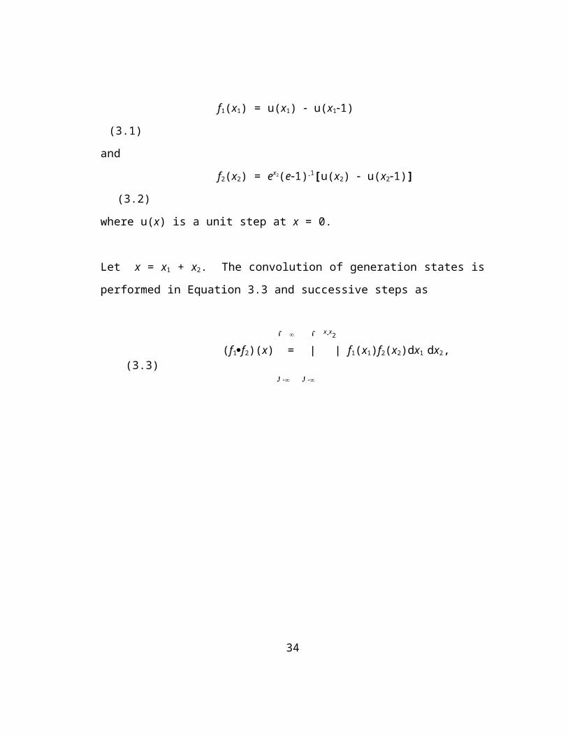
Piecewise Quadratic ConvolutionThe piecewise quadratic method was developed to improve interpolation

accuracy over the piecewise linear method. Preston and Grady in [34] have applied

the PQ method to the production costing problem and show the PQ benefits over

other mathematical formulations. Recently, Preston, Baughman, and Grady in [1]

use the PQ method to achieve high accuracy in the tails of line distributions. PQ

provides very low interpolation error in the right hand tail.

1F(x)

r

Pr

r = -1 r = 0 r = 1 -1 < r £ 0

0x: 0 1h (j-1)h jh (j+1)h ... nh

x in MW

Figure 3.20 Piecewise Quadratic Interpolation

The PQ method allows a set of discrete F( jh: j is an integer) points to describe

a continuous function using a quadratic interpolation process. Any three consecutive

points of F(x) are interpolated as shown in Figure 3.20 to provide a smooth and

continuous function F(x). The PQ interpolation is restricted to only the region

between the two left-most points of any set of three points to prevent the function

from taking on negative values on the right hand tail.

44

exact F(x)

Figure 3.20 illustrates how quadratic function interpolation is used to create a

continuous function from a set of discrete points at h intervals on the x axis. The

interpolation is performed within any range (j-1)h< x £ jh point in which j is an

integer meeting this requirement. Any real x is related to the discrete points using

x=h( j + r) for the range -1 < r £ 0. The piecewise quadratic interpolation equation

for calculating continuous real F(x) in Figure 3.20 for any real 0 < x < xmax is

F[( j + r)h] = .5r(r -1)F[( j -1)h] + (1- r 2 )F[ jh] + .5r(r +1) F[( j + 1)h] , (3.13)

which is derived in Appendix A.2.

Figure 3.21 below shows the interpolation needed for the PQ method’s down

and derated states shown in the Figure 3.14 pictorial. The PQ quadratic interpolation

is very similar to the PL linear interpolation process shown in Figure 3.18.

1 interpolated pointF(x)

hr hj

Pr

r = 1 r = 0 r = -1

0 0 1h (j-1)h jh (j+1)h ... nh

x in MW

Figure 3.21 Details For Piecewise Quadratic Interpolation And Shifting

45

approx. F(x)

The steps in setting up the j and r terms for PQ are the same as for PL. The

material is repeated here for completeness in describing the PQ process. In Figure

3.21 the function F(x) is to be shifted to the right by Ck and Dk MW to model the

generator Gk down and derated states, respectively. For each shift there is an integral

component of shift jh and a remainder of shift Dx. These shifts are related by

Ck=jch+Dxc and Dk=jdh+Dxd, respectively. Then the j values are jc=INT(Ck /h) and

jd=INT(Dk /h), and the remainders are Dxc=Ck-jch and Dxd=Dk-jdh. The interpolation

process uses a real per unit r to measure the partial distance remaining between

discrete increments. The per unit shift remainders are rc = Dxc / h and rd = Dxd / h.

Equation 3.14 for three state generators and Equation 3.15 for two state

generators are used to update each discrete F(x) point as a result of convolving each

generator k into F(x). These equations perform the scaling, shifting, and summation

as a single process for the convolving of each generator k into F(x). In this process,

no newly calculated values of F(x)+ on the left of each equation’s equal sign are to be

used in the right hand side of the equations. Any occurrence of F(x<0) = 1 and any

F(x³xmax) = 0. As each generator is convolved, xmax is increased by Ck MW before

the Equations 3.14 and 3.15 are applied.

Equations 3.14 and 3.15 use constant parameters that are recalculated for each

new Gk generator. The c0 ... d2, jc, and jd constant parameters used in (3.14) and

(3.15) are updated using the equations shown below for each generator. After these

are calculated, the convolution Equations 3.14 and 3.15 on the next page are stepped

through each integral value of j. Appendix A.3 shows how these are derived.

c0 = .5rc(rc+1) c1 = (1-rc2) c2 = .5rc(rc-1)

d0 = .5rd(rd+1) d1 = (1-rd2) d2 = .5rd(rd-1)

jc = INT(Ck / h) jd = INT(Dk / h)

46

The PQ convolution operation for a three state generator k is

[F{hj}+ = (1 - FORk - DFORk)×F{hj}

+ FORk×[c0F{h( j -jc-1)} + c1F{h( j -jc)} + c2F{h( j -jc+1)}]+ DFORk×[d0F{h( j -jd-1)} + d1F{h( j -jd)} + d2F{h( j -jd+1)}]

] " j = 0, jmax , 1 , (3.14)

which is derived in Appendix A.3. The PQ convolution operation for a two state

generator k is

[F{hj}+ = (1 - EFORk)×F{hj}

+ EFORk×[c0F{h( j -jc-1)} + c1F{h( j -jc)} + c2F{h( j -jc+1)}]] " j = 0, jmax , 1 . (3.15)

Note that the r<0 region shown in Figure 3.20 has a positive r pointing to the

right. However, the shifting to the right of Ck and Dk MW is more conveniently

written if the positive r direction is defined as pointing to the left. The sign change

defining positive r to the left as shown in Figure 3.21 has been factored into

Equations 3.14 and 3.15. This allows Ck = jh + Dx as well as r = Dx/ h to have all

positive numbers.

Equations 3.14 and 3.15 are represented symbolically with an · operator in

Equation 3.16 to represent the PQ convolution process.

[ F(x)+ = Gk·F(x) ] k = 1, Ng (3.16)

Note that the FG(x) generation reliability is calculated using Equation 3.16.

The line flow distributions F±j(x) have both positive and negative incremental flows

which are discussed in Chapter 8.

47

Calculating Piecewise Quadratic EUEThe expected unserved energy is the integral of F(x) from any real valued x to

¥ as shown by the shaded area in Figure 3.22. For x<0 let F(x)=1. The x is separated

into an integer j0 and a remainder r in preparation for the PQ Integral Equation 3.17.

1F(x)

j0h rh

Pr h

x

0 0 1h 2h 3h 4h 5h ... nh

x MW Generation Capacity Outaged

Figure 3.22 Integrating the PQ Function F(x)

The point j0h is located immediately to the left or exactly on x. Then j0 = INT(x/h)

and r = (x/h) - j0. The PQ equation for calculating EUE(x = SCk - y) in which y is a

constant load for one hour (i.e. load y = SCk - x MW) is

EUE[x = h( j0 + r)] = F x xx

( )d¥

ò MWh for 1 hr,

or in discrete form is

EUE[x] = [ F h j

j

j{ }

0

max + [-(r3/6) + (r2×3/4) - r -(7/12)] F{hj0} +

[(r3/3) - r2 +(1/12)] F{h( j0+1)} + [-(r3/6) +(r2/4) ] F{h( j0+2)} ]h. (3.17)

48

Integration using (3.17) is efficient computationally because the integration

process is a simple summation of F(x) discrete points plus an adjustment factor to

account for the left end effects of the quadratic. The unusual coefficients in Equation

3.17 arise naturally when Equation 3.13 is integrated. Starting with Equation 3.13,

substitute j0=j-1, j0+1=j, j0+2=j+1, and then integrate from r = -1 to r = 0. Figure

3.23 shows the area of integration. The x axis in Figure 3.23 is shown in terms of

discrete integers aligning with the discrete values of F(x). The integral between any

two discrete sections is shown in Equation 3.18.

1 F( jh)

j0 r

Pr

0 0 j0 j0+1 j0+2 j0+3 ... n

Figure 3.23 Integrating The PQ Function

Then

F jh jj

j( )d

0

0 1+

ò = [ 512 F(j0h) +

812 F((j0+1)h) -

112 F((j0+2)h) ]h . (3.18)

Integrating the rest of the h increments to the right of the one shown in Figure

3.23 produces a series of equations whose coefficients sum to one. Table 3.4 shows

this sequence of sets of three coefficients summing to unity.

49

Table 3.4 Summations Of PQ Integration Coefficients For Each Interval

j0 j0+1 j0+2 j0+3 j0+4

512

812

-1 12

this row integratesj0 - j0+1

512

812

-1 12

this row integratesj0+1 - j0+2

this row integratesj0+2 - j0+3

512

812

-1 12

512

812

512

11 12 1 1 1...

-7 12

+1 12

these are always added

- +1

6

3

43 2r r -r + -

1

33 2r r - +

1

6

1

43 2r r

these are added if

r > 0

The last row of Table 3.4 is the negative of the integral of from j0 to j0+r

which removes the area already added by the terms above the last row. The r term

allows integration from any real x to ¥. The overall integration process of a function

with hundreds of intervals is efficient in PQ format because a simple summation

process is used for all but three of the points.

1 Column j0 sums to 5/12 which is equal to 1-7/12.2 Column j0+1 sums to 13/12 which is equal to 1+1/12.

50

PQ InitializationEvery PQ distribution is initialized before proceeding with convolving the

outage states. The procedure for initializing PQ is similar to the piecewise linear

initialization shown in Figure 3.17 but is slightly more complex. Initializing the

generation outage distribution FG(x) is given in Figure 3.24. Figure 3.24a shows an

idealized initial condition for FG(x) before any generator outage states are convolved.

The PQ function cannot represent the step function, so an approximation is required.

Figure 3.24b shows an initial FG(x) with an expected value of zero initially.

1 1 A

Pr Pr p 713 ~.5

B0 0x:-2h -1h 0 1h 2h... x: -2h -1h 0 1h 2h...

Figure 3.24a Idealized Initial FG(x) Figure 3.24b Best PQ Initial FG(x)

The value of 713 is derived by differentiating A and B PQ equations using

(3.12), then finding the expected value of the density functions of A¢(p) and B¢(p) in

Figure 3.24b. Integrating rA¢ from r=-1 to r=0 and rB¢ from r=0 to r=1 shows that

the expected value is exactly zero when p= 713 . However, the use of p=.5 introduces

little error when PQ is compared with the ‘exact’ method. An argument is presented

on the next page that shows p=.5 initial value is favored when the initialization

procedure for line flow distributions is considered. The initial MaxGen configuration

line flows rarely align with an even grid increment.

Initializing a PQ function for transmission line j MaxGen configuration MW

flow requires finding a p that produces an expected value of the PQ function equal to 51

the MaxGen configuration MW load flow solution line flow. Figure 3.25 shows the

ideal and the PQ line function initializations.

i-1 i i+1 i-1 i i+11 1

A MaxGen MW flow xoj p xoj

Pr r Pr

B0 0

hj PQ F±j(x) grid i steps hj PQ F±j(x) grid i steps

Figure 3.25a Idealized Initial F±j(x) Figure 3.25b Best PQ Initial F±j(x)

The value of p in Figure 3.26b giving exactly the same expected value as the

step function in Figure 3.26a is p(r)=(12r+7)/13. Solving for the range of r shows

that p(r=- 713 )=0 and p(r= 1

2 )=1. However, the equation p(r)»(12r+6)/12 is

actually used as a close approximation. The line flow distribution error introduced

by this approximation is much smaller than other errors in the convolution process.

Figure 3.27 shows the two p(r) expressions plotted to scale.

1

exact p(r)

approximate p(r)=r+.50

r: -1 -.5 0 +.5 +1

Figure 3.27 Calculating Initial Line Distribution Parameter p(r)

52

- j is the number of h grid increments shifted- r is the remainder of an h grid increment shifted- positive r points to the left

Transmission line PQ distributions are initialized with their MaxGen

configuration MW flow xoj. Assuming the line’s grid step size hj has been

determined1, as well as the minimum and maximum ranges of the x MW flow axis,

then there is a grid increment in which xoj is less than or equal to half an hj distance

from the xoj. A single grid increment satisfying -.5<r£ .5 is identified. Use

r=[xoj/hj - INT(xoj/hj)] to find an r in the range 0£r<1. If r >.5, then replace r with

its complement r=1-r and initialize the next larger increment. Use the approximate

equation p=r+.5 to initialize this one grid increment. All lower index grid

increments are initialized to one, and all higher index grid increments are initialized

to zero1. By using the approximate equation for p rather than the exact equation, the

break points for r are nicely positioned halfway between the even grid increments.

The exact equation for p has a range of r greater than one, which creates confusion in

the selection of the appropriate grid increment to initialize. Therefore, the exact

equation is not favored by the author and is not used.

1 See Chapter 8 for more details on setting up the line distribution functions.

53

Chapter 4Solution Methodology

The experiences conveyed in Chapter 2 show that the composite generation-

transmission problem solution has been attempted using a number of mathematical

approaches. These experiences and their failures helped shape the thinking that has

gone into the PLF approach taken in this dissertation. Chapter 4 discusses why

certain solution approaches have been discarded. The last part of Chapter 4 outlines

a series of 27 steps that constitute the new PLF solution procedure.

Equivalent Versus Full Transmission Network RepresentationA theory for creating a network probabilistic equivalent model of a large AC

electric network does not exist. The network equivalents presented in the literature

[62,87] are equivalent impedance models in which specific lines in the real network are

retained while the rest of the lines are replaced with a set of equivalent impedances. The

literature does not describe how to set up the equivalent impedances to give equal

performance as limiting transmission elements with capacity constraints and failure

states. A probabilistic model using a full network representation avoids the issue of

whether the network being reduced has corrupted the solution. A network equivalent

must be newly created. If a full network model is used instead of an equivalent, then it is

readily available from each large region without further effort to create additional new

data.

The use of a network equivalent is driven by a need to increase the solution

speed so a larger number of generation configurations can be enumerated and tested.

The solution speed increase in the NARP program was not useful since most of the

transmission system was not represented in the equivalent, and no significant

transmission line overload events were observed.

54

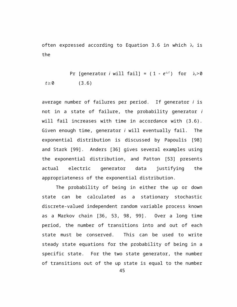
To allow more transmission detail in the equivalent, a new transmission

model was proposed to ERCOT based on the REI equivalent network [62,87] shown

in Figure 2.3. The REI adds many new links to make the incremental ‘tie’ flows

correct for each generation configuration. This new more detailed network model

still makes the assumption that the tie lines are sufficient for monitoring and

constraining the generation. It ignores the fact that many problems are frequently

associated with lines other than tie lines.

The more detailed REI equivalent has a new problem because of its size.

Computational efficiency is lost. The number of new REI links causes the load flow

solution matrix to lose much of its sparsity by creating a large number of new fill

terms during the matrix reduction and solution. The hoped for computational

efficiency of the REI is significantly diminished by the additional fill terms [97].

An example is given to illustrate the fill problem. The full matrix

representation of the 4300 bus 5200 transmission line example given in Chapter 11

typically has a maximum sparse matrix size of ~15,000 complex numbers using the

sparse techniques in [97]. An estimate of the REI number of links for the ERCOT

network with 300 power plants at 92 physical sites and 196 tie lines is shown in

Table 4.1. It has 2960 total lines and 196+196+92 = 484 buses in the reduced

network.

In a full network, the extra matrix fill terms are about equal to the original

number of off-diagonal terms. 4300 diagonal terms + 5200 upper matrix terms = the

initial full network matrix. Then the additional »5500 fill terms increase the matrix

size to about 15000 terms.

55

Table 4.1 Estimates for an ERCOT REI Model

Area Plant Sites Tie Lines Equivalent Lines

TU 24 45 1080

HLP 18 12 216

CPS 4 7 28

WTU 6 31 186

LCRA 8 19 152

STEX 16 13 208

COA 2 6 12

TMPP 14 63 882

Totals 92 196 2764+196=2960

How does the REI matrix compare? The initial REI has 484 (11% of 4300)

diagonal terms plus 2960 off-diagonal terms. If fill terms are assumed to be twice as

high in the equivalent, the final REI matrix has a total of 9364 numbers. This puts

the REI equivalent at about 60% the size of the full system matrix rather than at the

11% size based on the number of network buses retained in the equivalent.

The REI does not appear to be an attractive approach since the solution is

neither fast nor accurate. Loss of network information in the equivalent, small

savings in matrix size, and the extra work in creating the equivalent are good reasons

not to pursue this approach.

56

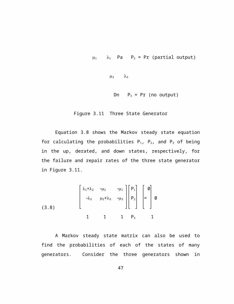
Generation Configuration Enumeration Versus ConvolutionThe enumeration of specific generation configurations is the most widely used

method of accounting for the effects of random generator outages in the composite

generation-transmission problem, as evidenced by the number of references using this

approach [3,5,6-29,31,36,56-95]. Interestingly, the opposite is true for the modeling

of random generator outages in power production costing studies. When

transmission systems are not considered, the convolution method is preferred [10,32-

54]1.

Enumeration is dominant in the composite generation-transmission models

due to the necessity for solving a deterministic electrical network matrix in order to

calculate the transmission line flows. The electrical matrix solution is not readily

solved for random variable inputs.

Convolution is widely used in production costing methods because the

computation speed is high and solutions are direct and unique. All the generation

outage configurations are modeled. Enumeration of generation configurations using

the Monte Carlo method (GENH and ENPRO) can require longer solution times than

the more direct convolution procedures (POLARIS, PROMOD, and PROSCREEN).

A simple example shows why direct enumeration of all generation outage

configurations is not computationally possible in a large system. Let a small system

have 100 two-state generators with Pr[on,off] = (.95,.05) for each generator. The

total number of configurations is 2100 » 1030. If 1000 configurations are evaluated

each second, the total run time for a single solution is more than 1019 years! If a

binary tree diagram is drawn for this problem on a flat sheet of imaginary paper with

one centimeter spacing between lines in which each line shows the status of each of

the 100 generators, then the diagram will stretch across a space of one trillion light

years. This is larger than the universe!

1 Chapter 3 gives an example showing the equivalence of convolution and enumeration.

57

An argument can be made that the uniformity of each generator’s states in the

100 generator example can be exploited, and the total probability of clusters of states

in which one, two, three, etc. generators are outaged at a time is easily calculated by

enumerating one state and using the results of the one state as the solution to a large

number of other states. However, real generators have different forced outage rates

and are physically located at different points in a completely non-homogenous

transmission network. Short-cut solution approaches are unlikely.

The real power flow distributions in every transmission line are strongly

determined by 1) line locations, 2) line outage states, 3) generator locations, 4)

generator capacities, 5) generator outage states, 6) locations of loads, and 7)

magnitudes of loads. Electrical networks are completely non-repetitive, non-

uniform, and non-homogeneous. The lack of a repetitive structure of the layouts of

the actual physical networks requires enumeration methods to spend more time

testing a system to find all the line overload configurations due to generation outages

and line outages.

Based on the discussion thus far, there seems to be no common solution to

two basic conflicting requirements. One of the requirements is a necessity to solve

the electrical network as set of specific configuration enumeration cases. Another

requirement is the need to exhaustively model the generation outage configurations,

which is not possible with the enumeration approach because too many

configurations exist to study all of them. Better sampling techniques are being

developed [3], but the author believes the configuration space is much too large and

irregular to make this approach successful.

The other solution possibility is to remove the necessity of using an electrical

matrix solution for calculating every new set of transmission line flows for every

generation and line outage configuration. This is the choice of the author because it

allows convolution to be used, which solves the problem of calculating the

immensely large numbers of generation outage configurations.

58

Transmission Line Flow Linearity RequirementsThe discussion thus far indicates that a full electrical network representation is

preferred, and convolution is the best way to cover all the generation outage

configurations. The convolution process requires linearity in the summation of line

flows. Line flows consist of both real and reactive power. The real power flows in

the network are strongly a function of all generators and loads throughout the

network. Reactive power flows are strongly related to local voltages, local shunt

inductance and capacitive sources, and the real and reactive power flow in lines. The

electrical network is reasonably linear in power if bus voltage magnitudes in the

network are nearly constant and real line losses are small. If voltage magnitudes at

regulated buses are held constant, the real power line flow distributions are almost

linear with respect to generation, loads, and line impedances. The linearity

characteristic is exploited in this dissertation to make the convolution approach

feasible. This is the reason all load flow cases for calculating incremental line flows

due to generator outages are solved with an unlimited reactive power at the

generation buses.

The network reactive power model is much more nonlinear than the real

power model because transmission lines have much higher reactive losses than real

power losses. In an actual system these line losses appear on each line and are

corrected locally. Transmitting reactive power through the network causes voltages

to increase or decrease from nominal levels, which is an undesirable characteristic.

Therefore, reactive compensation in the real world is best applied at distributed

locations where needed rather than transmitted from remote locations. An

insufficient amount of reactive generation available locally may result in voltage

collapse. A convolution model for non-linear reactive power has not been included

with the real power convolution model in this dissertation. The convolution method

presented in this dissertation cannot model the voltage collapse phenomena.59

The convolution method must have linearity in real power transmission line

flows. For example, if generator A is outaged and causes an incremental flow of X

MW in a transmission line; and if generator B is separately outaged and causes an

incremental flow of Y MW in the same line; then the simultaneous outaging of both

A and B generators must cause X+Y MW of incremental power flow in the line. If

the incremental power in each line is known for each generator’s outaged state, and

the incremental line flows are linear for multiple generators outaged, then simple

summations can be used to estimate the power flows in all lines for any configuration

with several generators outaged.

The convolution approach requires1 the sum of all the incremental line flows

due to all generators and all loads (+ losses) be in agreement with a full network AC

load flow solution with all generators running at maximum capacity. This is a unique

configuration since it defines the maximum amount of load (+ loss) that can be

served and is given the name MaxGen. Load levels greater than the MaxGen

configuration are unserved.

Another unique configuration is the one with all generators in a state of

failure. This configuration serves no load and has nearly zero real power line flows.

The zero load configuration is of lesser importance since line overloads generally do

not occur at low load levels. Also, the total probability of having most of the

generators outaged is small.

A MaxGen configuration load flow is set up and run first. Then additional

load flows are run as variations of the MaxGen configuration case in which a single

generator is outaged for each new load flow case. This allows all the incremental line

flows for each generator outaged to be calculated by subtracting the results of each

case from the MaxGen case. These incremental flows are normalized and stored in

an Hj,k matrix of lines j and generators k for use in enumeration and convolution

1 Required because the sum of all outages must produce zero MW line flows.

60

operations. In creating this matrix, the individual load flow solutions need to be

solved to a very tight tolerance to minimize cumulative line flow errors when

summing large numbers of small incremental flows. The author’s experience

shows .01 MW maximum power mismatch at each bus in all the solved load flow

cases produces sums of distributions with less than 1% error whereas .1 MW

maximum power mismatch at each bus has been observed to produce as much as 15%

summation error for the ERCOT system. This summation error is easily observed at

radial generator buses with no load. The error being discussed here is prior to any

scaling or adjustments to minimize the overall error in summing the incremental

flows on each line.

The matrix of incremental line flows can be used to estimate the total line

flows for any specific configuration of generators outaged. An enumeration approach

using this matrix to cover all generation outage configurations is not feasible because

far too many configurations would need to be calculated. Convolving the individual

generator outage states is feasible and was covered in Chapter 3. The convolution

process produces cumulative line flow distributions that closely approximate the

distributions that would have been calculated if all combinations of generation outage

states were fully enumerated.

61

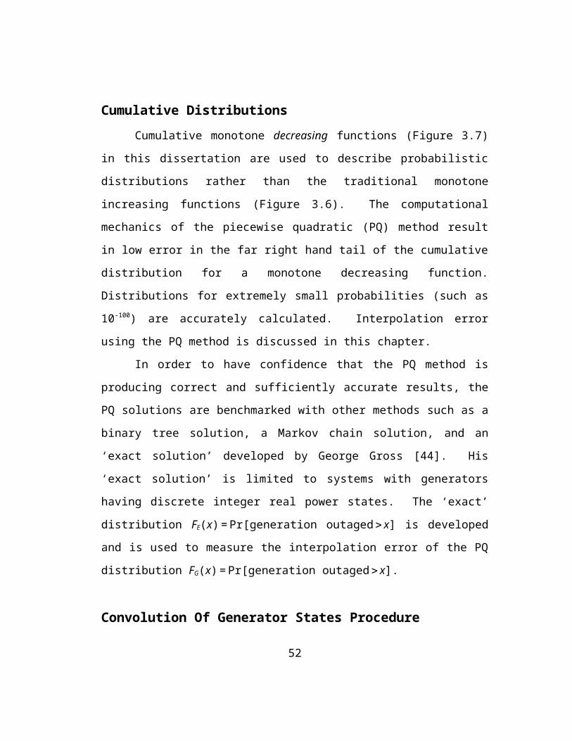
Load Model ConsiderationsThe MaxGen configuration load flow and generator outage load flows are

used to calculate a matrix of generator-line distribution factors [1,29,55] for

calculating the incremental line flows associated with generator outage and derating

states. When a generator is outaged in a load flow: 1) other generators must increase

their power output, or 2) load must be reduced. The total generation power must

exactly equal the total load plus total losses at all times in every load flow solution.

Load and generation can be adjusted an infinite number of ways to meet the

total power requirement when a generator is outaged. Some of the possible

adjustments are conditional. An example of conditional dispatch of power is when

power can be made available to a load area when another area does not need the

power. This situation requires a more complex conditional probabilistic convolution

process. Some production costing programs use a series of convolutions and

deconvolutions to model one type of conditionally probabilistic dispatch of

generators. The deconvolution process is difficult to implement, is numerically

unstable, and is computationally time consuming. The convolution approach here is

to treat all generator outages as independent events. The formulations requiring

conditionally probabilistic events will not be modeled in this dissertation.

The usual enumeration model approach for replacing the capacity of an

outaged generator is to increase the power on the other generators. The physical

system also responds in this manner when a generator fails. Other generators

increase output power to make up for the lost capacity, which can occur if surplus

capacity is available. If no surplus capacity is available when a generator is outaged,

loads must be reduced to keep the network operational.

The PLF model load+losses MW is always set equal to generation MW and

the generators are always run at maximum output for every generation outage

configuration.

62

There is never spare generation capacity in this solution process. The only

response possible in the PLF model is to initiate load reductions as generators are

outaged. If the PLF had been designed to model spare generation capacity,

conditional probabilities would have been needed, as well as a definition of how

spare capacity is to be shared in the system. The mathematical formulation and

definitions would be more complex and harder to follow than what is presented here.

Some of the information required to define the conditional dispatches has yet to be

completely and uniquely defined in the real world operational practices.

Generation outaged in this convolution model always results in a load

reduction. The amount of reduction and the location of load reductions should be

optimally calculated to minimize the total loss of load. One important requirement in

using the convolution method with any load reduction scheme is to insure that the

sum of all incremental load reductions are consistent. The sum of loads shed at any

bus cannot exceed the total load on that bus in the MaxGen configuration load flow.

This condition is stringent enough to eliminate the use of a single generator slack bus

in the load flow. Two basic methodologies for executing load shedding (load

reduction) are LLS for load loss sharing and NLLS for no load loss sharing.

Load Loss SharingThe PLF model presented here is consistent with single area reliability results.

Single area reliability analysis calculates the total system generation adequacy.

Unserved load occurs when random generator outages cause generation capacity to

drop below the total system load level. A measure of reliability is the probability of

being generation deficient in serving the total system load. Individual area

generation reliability is not calculated.

The simplest extension to the single area model in creating a composite

generation-transmission model is to calculate the additional decrease in the total

63

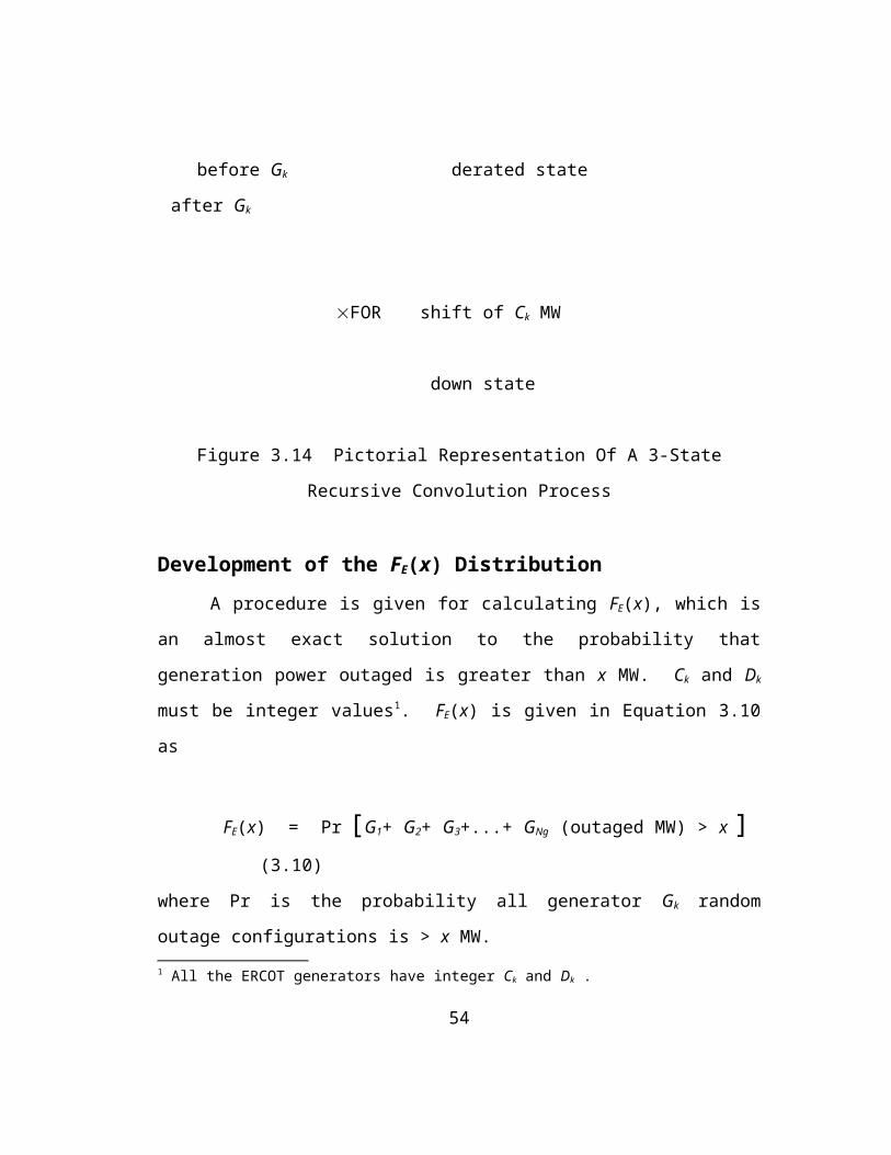
single area reliability imposed by the transmission system. The idea here is that

every bus in the network has the same physical reliability as the system as a whole if

no transmission constraints exist. This definition allows transmission constraints to

be calculated as a simple extension to the single area analysis.

Note that this is a physical interpretation of the system rather than a legal

interpretation. Contractual agreements between individual load areas can change the

reliability of generation supply to each area. The modeling of supply contracts and

their effect on the reliability of generation in each area is beyond the scope of this

dissertation and will not be considered here.

The discussion presented on this page thus far is consistent with a load loss

sharing (LLS) methodology. Why is this so? Because the only way to have exactly

the same generation reliability on every bus in the network is to probabilistically

dispatch every generator to all buses in the network on an equal basis. Every bus

load gets a small prorata share of each generator’s power. This uniquely defines how

the loads in the network are to be scaled for each case with a generator outaged. The

entire system load is linearly scaled to account for both the drop in generation power

in the network as well as the change in losses. No load flow slack generator is used.

No Load Loss SharingThe NLLS methodology allows owners of generators to have first call on

their own generation capacity. Conversely, when a generator is forced out of service,

the owners of the outaged generator(s) will have their loads shed unless other surplus

generation capacity exists in the system. Surplus generation is used by load areas

needing capacity but the sharing methodology for surplus capacity is not well

defined. The NLLS load model is conditional on the availability of surplus

generation. The surplus generation is only available if other areas are not using the

generation and the overall generation exceeds the total system load.

64

The NLLS methodology has problems that prevent it from being used in the

PLF model in this dissertation. The most important problem with NLLS is the very

definition of generation reliability the NLLS creates. The NLLS does not result in

every load bus receiving the same generation reliability as the single area reliability.

Each area’s load buses become a function of the FOR’s of each area’s owned

generators. Individual contracts between companies and complex operating rules

would need to be a part of the input data in the NLLS model. This data is not

presently used in regional studies and would be difficult to obtain.

The NLLS is not a simple extension of the single area analysis. The NLLS is

a new measure defining a different reliability for each area even though no

transmission constraints are included. Adopting the NLLS load model here would

result in the need to develop a new mathematics based on conditional probabilistic

convolution. This topic has not been presented in the literature and constitutes a new

area of study separate from the transmission model developed here. The NLLS

convolution model may not be mathematically possible. The NLLS model will not

be used in this dissertation for these reasons.

65

Measuring Single Area (Total System) Generation ReliabilityThe reliability of the total system generation is measured in terms of a

function FG(x) which is the probability that the total generation outaged is greater

than x MW. Figure 4.1 shows FG(x) for the 286 generator test model. As an example

of how to read Figure 4.1, one could say there is a 10% probability that more than

14% of the total ERCOT generation MW will be out of service.

.0

.1

.2

.3

.4

.5

.6

.7

.8

.9

1.0

0 1 2 3 4 5 6 7 8 9 10 11 12 13 14 15 16 17 18 19 20 21 22 23 24 25

<=Max Load (x MW outaged - % of total capacity) Min Load=>

Pro

babi

lity

Figure 4.1 Probability Outaged MW > x

In this dissertation the FG(x) definition is extended to mean the relative

generation reliability at every load bus in the network. This definition is a physical

interpretation of the system in which the network is constrained by the total

generation capacity and reliability and by the capacities and reliability of the

transmission system. Loss of load due to generation is shared proportionately on all

load buses. This requires a generation supply load loss sharing (LLS) methodology.

Although the generation supply is applied uniformly to all load buses, the

transmission system constraints caused by individual lines requires the load sheddings 66

quadratic interpolation is restricted to the left-most two of the three consecutive points to avoid negative F(x) (see below)

due to line overloads be performed on the basis of specific generation and loads in

the network that are the most responsible for causing the line overloads. The

generation-load pairs that are the best candidates for load sheddings are listed in

descending order in a load shedding table (LST). Frequently the entries in the LST

have exactly the same ability or benefit in unloading overloaded lines. This creates a

sharing and allocation solution problem similar to the NLLS problem previously

discussed. There is an element of non-uniqueness in the load shedding solution that

cannot be avoided unless more loss sharing information is supplied.

In addition to the FG(x) as a measure of the probability of being capacity

deficient, a better indicator of reliability is the expected unserved energy, or rather

the EUE(x) as a function of the load x MW1. The EUE(x) is the integral of FG(x)

from x to ¥ and is used to cover a one hour period (in this dissertation). Frequently

the EUE is calculated for an entire year, which includes all the operational data such

as generator and line maintenance schedules and hourly loads, but the transmission

system reliability is best measured at the highest load level in which there is no

scheduled maintenance. Limiting the analysis to peak load periods simplifies the data

gathering process and allows the user to study the primary problem rather than be

burdened by unimportant data. Also, the solution time for solving an entire year with

maintenance schedules would be at least ten times greater than the approach taken

here. Therefore, the author has elected to calculate the transmission system reliability

and the transmission system’s effect on generation reliability only at the peak load

periods.

1 Note that the maximum load occurs for zero outaged generation MW as shown in Figure 4.1. The load level is equal to the total generation capacity minus the generation outaged.

67

Deterministically Removing Line OverloadsThe removing of line overloads is the last step in the solution process after all

probabilistic line flows due to all generator outages have been calculated. To

understand this process requires a knowledge of the relationship between specific line

flow states and generator states. If a binary tree diagram is constructed for all the

configurations of the generation states, then there is a unique line flow state for every

configuration. Figure 4.2 illustrates this by showing that generator configuration

with probability p in the binary tree has a unique location on both the generation

outage distribution and on the line flow distribution.

Pr p Pr

p

Gen. States MW MW

p Generation States FG(x) Line Flows

Figure 4.2 Generator Configuration With Pr p Is Shifted To Reduce Line Loading

The figure shows how a shift in the line flow p configuration to the left

corresponds to a unique shift of the same p configuration to the right in the generator

outage distribution. On the binary tree a single generator out of many is identified

and is reduced in MW output, and this effectively causes the MW shift of p in the

two distributions. All the lines in the network will each have a shift in the p

configuration in the same manner as shown for the one line in Figure 4.2.

68

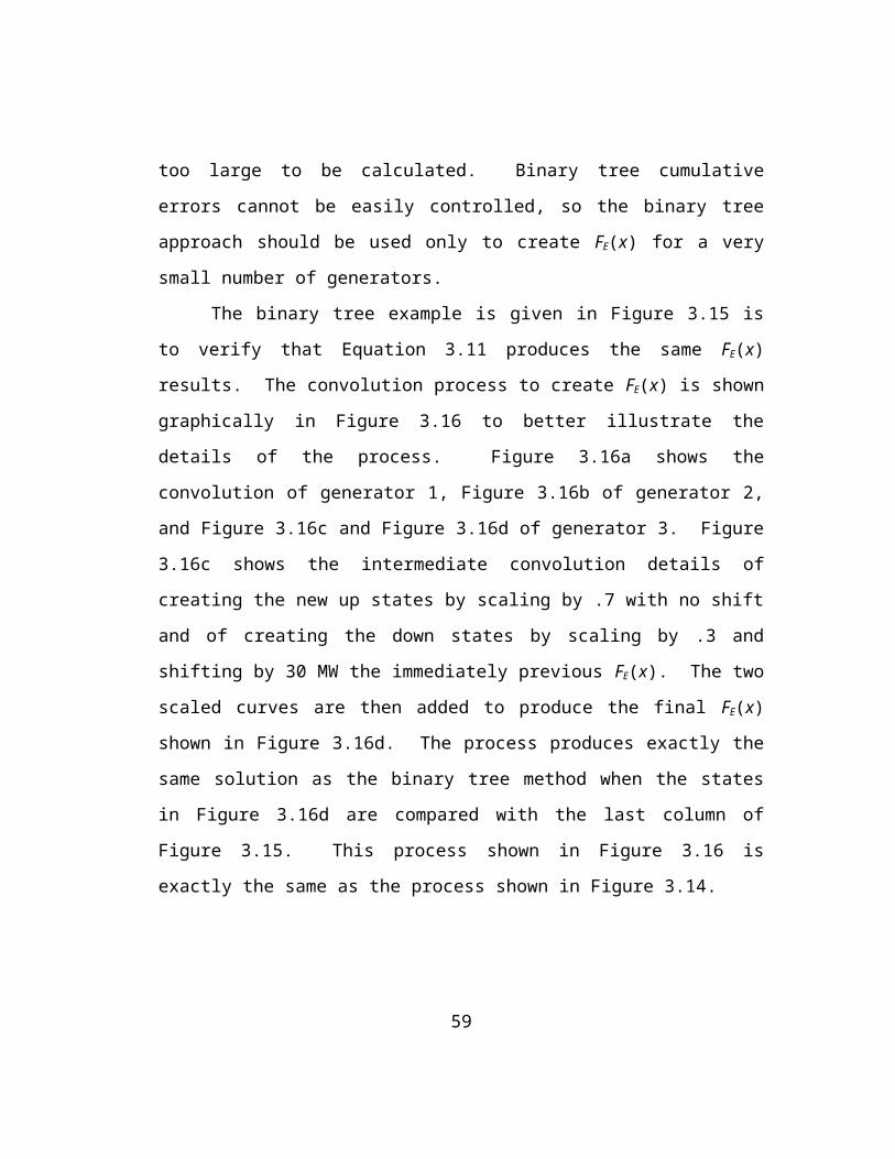
Measuring Multi-Area Generation And Transmission ReliabilityMultiple load areas are part of the load flow set of data. Each bus in the

network is assigned to an area. There may be any number of areas in the load flow,

except each area must have at least one bus specified within the area. The load MW

within each area is the sum of all the bus loads within the area. The load within each

area in the original load flow data is scaled so that the MaxGen configuration load

flow area loads are equal to owned and purchased generation capacity.

The generation reliability within each area is defined as being the same FG(x)

function as the example shown in Figure 4.1, except the x axis of this function is

scaled to represent the total load within each area. The percentages shown on the x

axis in Figure 4.1 become the percentages of unserved load for each area from the

MaxGen load for each of the areas respectively. In this manner each area receives

the same level of generation reliability before transmission constraints are applied.

Transmission constraints are reduced when the line overloads are

deterministically shifted as shown in Figure 4.2. For each specific state with

probability p that is shifted, a real generator and a ‘virtual generator’ are matched to

create a generator-load pair that is reduced in MW level so that the corresponding p

state causing the line overload is shifted to a lower level of overload for the line. The

reduction in MW for probability p is mapped back to the total system FG(x) and to the

local load area’s FG(x). In this manner, the decrease in reliability due to transmission

constraints is assigned to specific load areas.

The virtual generators mentioned above are injections of power at load buses

in which the load is to be reduced. Real power incremental line flows from virtual

generators are combined with real power incremental flows from the generator to

produce incremental line flows equal to the incremental flows seen in an AC load

flow in which the generator and area load are simultaneously reduced.

69

Summary Of The PLF Solution ProcedureThe steps of the PLF solution procedure to evaluate the generation outage

states using convolution and the transmission line outage states using enumeration are

given below. Details are given under each step, except the mathematical details of

the load flow procedures, the convolution mathematics, and the procedures for

shedding loads are covered in later chapters.

Step 1. Read all the input data into a computer program, then in the program, scale

loads to match total generation supply, and solve the MaxGen configuration load

flow. The input data consists of the usual load flow data for the large area plus the

generator data of FOR, DFOR, maximum capacity, and derated capacity. Appendix

D.1 shows an example of the load flow and generator input data. After the data is in

the computer program, the bus loads in each area are scaled to matched owned and

purchased generation for each area. This sets up the required ‘MaxGen

configuration’ load flow condition in which no generators are outaged, and a

maximum amount of load is being served. The regulated buses maintain specified

voltages with no reactive constraints. Lines may be overloaded in the MaxGen

configuration load flow case. Corrective actions are taken later in Steps 10-20 after

the probabilistic line flow distributions have been calculated.

Step 2. Calculate FG(x), which is the reliability of the total system generation

supply without transmission constraints. Convolution of all generator outage states

produces the FG(x) function. Chapter 3 presented the mathematical details of the

convolution process. The FG(x) function x range is scaled to match whatever

70

maximum load is being served. For the total system, the x is set to measure total

system MW load at x=0 down to zero MW load at x=xmax . This is the normal scale

71

for the abscissa of FG(x). Likewise, for any load area or any load bus, the x axis is

scaled to measure the maximum MW load at x=0 down to zero MW load at x=xmax .

This is equivalent to calculating the reliability of generation supply at every bus in

the load flow separately. Since the reliability of generation supply is the same

throughout the network before transmission constraints are considered, the FG(x) is

scaled to represent that same reliability rather than actually performing the

convolution of generation states for every load bus.

Step 3. Run single generator outage cases to calculate incremental line flows

associated with each generator outage. These are found by subtracting the generator

outaged case line flows from the MaxGen configuration real power line flows. The

incremental flows are stored in array Hj,k for lines j and outaged generators k. To

perform Step 3, the generator outaged load flow case is modified from the MaxGen

case by uniformly scaling down the bus loads across the network to account for the

outaged generation capacity. To eliminate the need for a slack bus, the total system

loads are also scaled during the load flow solution to account for incremental losses.

Step 4. Run virtual generation incremental cases and append the results to Hj,k. The

virtual generation incremental line flows are calculated in this step but are not used

until Step 11, which is the load shedding operation. Individual load flow cases are

set up and solved for each virtual generator case. One virtual generator case can

represent load shedding on a single load bus or on a group of load buses such as an

area. The PLF program models the virtual generation incremental flows by

effectively increasing all the loads in an area by 50% and at the same time decreasing 72

the total network loads. Note that the 50% increase in loads are stored in a separate

array from the regular bus loads and are held constant throughout the load flow

73

solution. All bus loads are uniformly scaled downward to meet the total power

requirement. This includes scaling the load shedding buses also. The load flow is

solved the same as in Step 3 by adjusting all loads proportionately to account for the

total system real power loss. The PLF program calculates virtual generation for

every area rather than every bus in the network. This allows load shedding to be

done uniformly within each area. Load areas in the PLF can be defined as small as

necessary to represent any level of load shedding detail desired in a study.

How these load shedding areas are defined has a very large effect on the load

shedding energy for each area. The most detailed model representation possible is to

treat every substation (that has a load) as a separate virtual generator for load

shedding. This level of selective load shedding will minimize the overall EUE load

shed because load is shed closest to the overloaded line. However, the computational

effort to have a virtual generator at every load bus is large. A faster approach is to

assume a lower bound on the line distribution factor. This assumes that a load

somewhere in the vicinity of the overloaded line exists with the distribution factor

equal to the lower bound. The EUE will be minimized using this approach without

modeling virtual generation at every bus. The PLF program can be run either with

any level of detail in defining load areas or can be run with a lower bound on the line

distribution factors.

Step 5. Adjust the dominant Hj,k MW flows to improve linearity. The sum of all

generator outage incremental real power flows in Hj,k should produce MW line flows

in agreement with the MaxGen configuration MW flows on all the transmission lines.

74

However, due to nonlinear load flow solutions, the sum of incremental real power

flows in a line is only an approximation to the actual MaxGen configuration flow.

On every line, the sum can be adjusted to agree exactly with the MaxGen

configuration flow by slightly adjusting the Hj,k line flows calculated in Step 3.

Experience shows the adjustments are usually small. In the systems tested in this

dissertation, the average correction is one to two percent of the line ratings on

average. The total MW flow in each line is the sum of many incremental flows in

both directions on each line. The major incremental flows in the same direction as

the MaxGen configuration flows are called the ‘dominant’ incremental flows. The

operation performed in Step 5 scales only the dominant incremental flows so that the

sum of all incremental flows agrees exactly with the MaxGen configuration flow.

Each line is adjusted as a separate operation.

Step 6. Normalize the real MW incremental flows in Hj,k to per unit values by dividing

each Hj,k term by the MW real generator Ck or by the virtual MW generation.

Step 7. Discard analysis on lines that will not overload at all. Define a direction of

flow on each line as the positive direction. Negative is in the opposite direction.

Then sum separately the positive and negative incremental flows on each line. If

both the positive and negative flow sums for a line are less than the line rating, then

the line will never overload for any generator outage configurations. Lines that have

positive and negative flow sums less than their line ratings can be discarded from

further analysis, since they will never overload for any generation outage

configuration. 75

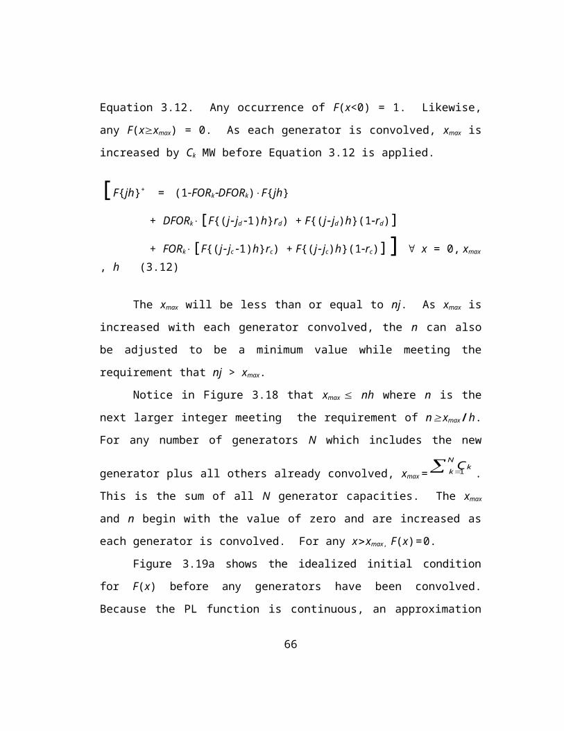
Step 8. Calculate line flow distributions F±j(y). The probabilistic line flows are

calculated in a manner similar to FG(x), except the convolution is performed twice to

maintain convolution solution accuracy. The PQ process for calculating the line

distribution is accurate only in the right hand tail. Since the left hand tail also

contains line overloads, the convolution must be repeated with all incremental line

flows reversed in direction. All incremental flows are convolved once in the +

positive direction and again in the - direction.

Convolution mathematical details using a piecewise quadratic functional were

given in Chapter 3. In summary, the incremental line flows are convolved together

on each line using each generator’s state probabilities to produce a set of line flow

distributions. The line flow distributions are the F±j(y) calculated in this step. Since

the lines with no possibility of overload have already been eliminated in Step 7, every

line in Step 8 is overloaded. All the F±j(y) distributions calculated in Step 8 will have

a portion of their right hand tail of the distribution function extending beyond the line

rating as illustrated in Figure 4.3.

1

Pr

0

- rating 0 MW + rating76

positive r points to the right

Figure 4.3 An Example Of Probabilistic Line Overload

Step 9. Discard analysis on lines with low overload probability. Many lines will

have an extremely small probability of overload in the right hand tail of F±j(y). Lines

with probability of overload less than 10-12 can be eliminated. This probability of

overload is too small to affect output results.

Step 10. Choose line j with the largest probability of overload (flow distributions

are calculated in Step 8). Choose a small increment of Dy MW on this line to unload.

The Dy increment has an average probability p. Step 20 shows why the line j

probability must be the largest. This is the first step in a process of removing line

overloads from all the F±j(y) for lines that have not been discarded in Steps 7 and 9.

Chapter 10 gives a more detailed explanation of the processes in Steps 10-20. The

steps below are only a summary.

Step 11. Create a load shedding table (LST) for line j if it has not already been

created. The real generator Hj,m distribution factors for line j and the virtual generator

Hj,n distribution factors (in Chapter 7) for line j are combined using Hj,m-n= Hj,m - Hj,n

linear superposition to create all combinations of generator-load pairs of distribution

factors Hj,m-n for line j. The combined factors that have the greatest positive values in

the direction of line overload are the generation and load combinations that are

mostly causing the line to be overloaded. An LST is constructed in which the

greatest factor generator-load pair is at the top of the list, the next greatest factor is

second, and so on. The LST is a table of generator-load pairs in which the factors are 77

sorted in descending order from greatest benefit to least benefit in being able to

unload the overloaded line j.

Step 12. Recalculate the line distribution function Fj(y) for line j using only the Hj,k

generator flows causing an increase in overload. This step partitions the generators

contibuting to the overload and those reducing the overload into two sets. The line

flow distribution is recalculated in Step 12 using only the generators contributing to

the line overload1. These are referred to as increasing flows. These increasing flows

are convolved together to give a distribution that is only a function of generators

causing the line to be overloaded. The line overloads due only to the generators

causing the overloads are shown in Figure 4.4. If the decreasing flows are convolved

into the function shown in Figure 4.4, the original flows causing overloads are

scattered across the functions. Their locations are no longer identifiable, as shown in

Figure 4.5.

1 1

s ame Pr, Different MW

Pr Line Rating

0 MW 0 MW

Generation Outage States FG(x) Line j Flows

Figure 4.4 Line Distribution Due Only To Increasing Flows

1A detailed explanation for the necessity of this step is given in Chapter 10.

78

- j is the number of h grid increments F(x) is shifted to the right- r is the remainder of an h grid increment for shifting F(x) right- positive r points to the left

1 1

s ame Pr, MW Locations Are Lost

Pr Line Rating

0 MW 0 MW

Generation Outage States FG(x) Line j Flows

Figure 4.5 Shift In Line Overloads With Decreasing Flows Included

79

Pr

Figure 4.5 shows that the original line j overloads in Figure 4.4 cannot be

exactly located in the generation outage states distribution after the decreasing flow

generators are convolved into the function. A new function F(x,y) is used in Step 18

to locate the line j overloads after decreasing flows are convolved.

Step 13. Use the Fj(y) of increasing flows to initialize F(x,y). The F(x,y) will

allow three measures to be directly linked together so changes in one can be mapped

to the others. These are: 1) line j overloads, 2) specific generation-load pairs to be

used in the shedding of load, and 3) the incremental changes to FG(x) caused by

removing the line overloads. Figure 4.6 shows an example of the initial F(x,y) which

consists of only the increasing line flows.

y

1

Pr

0

of increasing flow gen.

direction of shifted states in Step 14

FG(x) is inverted and x axis is reversed x

of all generation MW

Figure 4.6 An Example Of Initial F(x,y)

80

FG(x)

Step 14. Convolve the decreasing line flow generators. The convolution of

negative flow generators into F(x,y) causes the line overloads to shift downward in

the negative y direction in Figure 4.6 and, at the same time, shift in the positive x

direction. Figure 4.7 shows how F(x,y) may appear after these convolutions. Step 15

will begin a process of identifying individual load shedding distributions.

y

1

Pr

0

increasing flow gens.

FG(x) is inverted and x axis is reversed x

of all generation MW

Figure 4.7 An Example Of F(x,y) With All Generators Convolved

Step 15. Convert F(x,y) to a partial density function Fp(x,y) by subtracting adjacent

x rows for all y. Fp(x,y) = F(x,y)-F(x+hx ,y) where hx is a discrete grid spacing. The

reason F(x,y) in Figure 4.7 is converted to a density function is to identify the

specific line j overloads associated with each x MW load level. Then later in Step 18

(see Figure 4.8) the Fp(x,y) are moved across the surface of the x-y plane along a path

of slope Dy/Dx equal to the normal generator-load transmission line j real power

distribution factor Hj,m-n.

81

overloaded

Step 16. Select the next generator-load pair from the LST to be used in reducing

the line overloads. This is an initial step for the load shedding operation. The

shifting of flow distributions in the F(x,y) space is the load shedding process.

Generation-load and line j overloads are simultaneously reduced as a deterministic

process.

Step 17. Calculate the maximum MW reduction needed for this generator-load

pair. The MW needed to unload the line may be less than the generator’s capacity.

Also, the maximum Dy line MW shift is limited in order to retain the line j status as

the line with the highest probability of overload.

y

1

Pr

0

increasing flow gens.

x

of all generation MW

Figure 4.8 Shifting The Line Overloads To The Generation/Load Axis - x

Step 18. Shift the Fp(x,y) partial distributions as a function of the load shedding

MW generation and the generator-load distribution factor as shown in Figure 4.8.

82

F±j(y)

The shifting process folds the distributions from the y axis to the lower x axis. What

is happening here is that all the distributions are being shifted down and to the left

with a slope equal to the line real power normalized distribution factor, Hj,m-n. The

distributions are not moved beyond the lower x axis (which is also the line j MW

rating of Rj). Also the distributions are not shifted beyond what will allow line j to

have the highest probability of overload. This process causes the line distributions to

be ‘folded’ onto the x axis. The process of shifting these distributions creates the

load shedding information and this is stored in a temporary array T(x). The T(x)

array is then added to the generation reliability FG(x) and reset to zero for the next set

of line overloads after Step 19.

Step 19. Calculate the incremental changes in FG(x) from shifted Fp(x,y). The

incremental distributions in T(x) are added to FG(x) as shown in Figure 4.9 (also see

Figure 4.1). This is the additional decrease in reliability caused by the line j

constraints.

1

Pr

0

Figure 4.9 Generation Unreliability Due To Transmission Constraints - T(x)

83

overload

Step 20. Estimate the reduction in loading of other overloaded lines due to the line

j Dy MW. The shifted increments on line j are due to the m-n generation-load pair

reducing their MW by an amount Dy/Hj,m-n at a probability p. Line j overload

increments are reduced by Dy MW. This generator-load pair may be contributing to

the overloads of other lines l. Each of these other overloaded lines l will have a

smaller (but positive) Hl,m-n distribution factor. All the overloads in the other lines are

decreased by an amount equal to (Dy)(Hl,m-n)(Hj,m-n)-1 provided that line j has a higher

probability of occurrence than the other lines l. This approximation assumes line j

overload event(s) are coincident in time with the other line overloads selected.

Step 21. Repeat steps 16 through 21 for each Dy increment until line j no longer

has the largest probability of overload. Repeating these steps allows more entries in

the LST to participate in the load shedding and line overload reduction process.

Usually many generators and loads are needed in the load shedding process to

completely remove all the probabilistic line overloads. The line overloads tend to

have extremely small probabilities at very large MW overloads.

Step 22. Repeat steps 10 through 22 until no more lines are overloaded. After each

line j is unloaded, and all the other lines l have been adjusted as a result of all the

lines unloaded up to the line j being unloaded, other lines are usually remaining to be

overloaded. A new line j is selected in 10 as a candidate for having its line overloads

removed. This process is continued until no more lines with overloads are present.

84

With each line being unloaded, the process of adding the T(x) to FG(x) is cumulative.

Other statistics are collected for each line that is unloaded.

Step 23. Calculate the probability of this transmission configuration and save other

statistics for this transmission configuration. The first transmission configuration is

all lines in service. Other transmission configurations will have one or more lines out

of service. The probability of the individual line outage configurations is conditional,

based on the amount of transmission probability space examined. If a group of lines

in the network are selected for study, the probabilities of all the transmission outage

events are made conditional to the outages modeled, such that the total transmission

outage space probabilities will sum to one. Chapter 11 shows that the enumeration of

double simultaneous transmission outage events covers most of the total probability

space of line outages.

Step 24. Select a line outage configuration to enumerate or go to Step 27 if all

desired line outage configurations have been modeled. Note that the first

configuration modeled has all lines in service. Line outages are simulated explicitly.

There is no direct convolution process that will model incremental probabilistic line

flows as a result of outaging other lines with probabilistic flows. So the entire solution

process is repeated for each specific line outage configuration, and load shedding

statistics are recorded for each line outage configuration.

Step 25. Test for system separation using complex injection currents. Chapter 9

gives the mathematical details for this test. If a system separation has occurred

85

because one or more lines are outaged, record the probability of this configuration

and return to Step 24 for a new line outage configuration. The study of dynamic

processes due to system separation is beyond the scope of this dissertation.

Step 26. Adjust Hj,k factors for the specific line outage configuration and repeat

Steps 7-23. The real power line outage distribution factors are updated through an

efficient mathematical process described in Chapter 9.

Step 27. Prepare final output reports and end the program run.

86

Chapter 5

Generation Reliability

Chapter 1 introduces the idea that present day computational tools are

inadequate for solving the composite generation-transmission reliability problem.

Chapters 2 and 4 state that this lack of success is due to a reliance on enumeration for

testing the extremely large number of generation outage configurations. Generation

reliability programs today are successfully using convolution as a means of modeling

the generation outage events exhaustively for problems with simple radial

transmission networks (MAREL and GRIP) and no electrical network at all (UCS).

The success of the convolution approach for modeling generation outage

events is retained in this dissertation and is extended to include the full transmission

network. To use convolution in a large transmission network model requires linearity

of line flows in the electrical network as well as a tractable definition of the

generation reliability. The discussion in Chapter 4 indicates that proportional LLS is

consistent with convolution and the uniformity of generation reliability at every bus

whereas the NLLS is inconsistent with both. Consideration of LLS versus NLLS is

of primary importance and is discussed further in this chapter. This chapter also

discusses: the conversion of three state generator data into two state generator data;

the error of FG(x) compared with FE(x); the definition of generation reliability used in

this dissertation versus other definitions for calculating LOLP and EUE; and why a

load model is not explicitly included in the composite G-T model presented here.

Figures 5.1a (linear probability scale) and 5.1b (logarithmic probability scale)

show an example of FG(x), the probability that generation outaged is greater than x

MW, for the ERCOT 286 generator system. The total generation is 58,197 MW and a

1% grid step size, h=58.197 MW, is used. The curves in Figure 5.1 have been

calculated using the PQ convolution mathematics presented in Chapter 3.

87

.0

.1

.2

.3

.4

.5

.6

.7

.8

.9

1.0

0 1 2 3 4 5 6 7 8 9 10 11 12 13 14 15 16 17 18 19 20 21 22 23 24 25

<=Max Load (x MW outaged - % of total capacity) Min Load=>

Pro

babi

lity

Figure 5.1a Probability Outaged MW > x

1.E-14

1.E-12

1.E-10

1.E-8

1.E-6

1.E-4

1.E-2

1.E+0

0 2 4 6 8 10 12 14 16 18 20 22 24 26 28 30 32 34

<=Max Load (x MW outaged - % of total capacity) Min Load=>

Pro

babi

lity

Gen

erat

ion

Is U

nava

ilabl

e

Figure 5.1b Probability Outaged MW > x

88

line j overload states in Fig. 4.4+ rating £ y £ max. line flow

F(x,y)overload

F(x,y) surface as a set of discrete points

line overload states as shown in Fig. 4.5

The PLF computer code used in this dissertation was initially written for two

state generators. Code sections with a two state generator model included: 1) the

convolution of generation outage states; 2) the convolution of line flow states; and

3) a linear program for minimizing load shedding in enumerated solutions1. Three

state generator representation has recently been included in section 1), but has not

been included in sections 2) or 3) listed above. Three state generator studies cannot

be run until the section 2) computer code has been updated. Since the ERCOT data

contains both two and three state generators, a two state approximation to the three

state generator data is presently required to run the existing computer program. A

two state EFOR from three state generator data has been included in the computer

code and is shown in Equation 5.1 as

EFORk = FORk + DFORk×DC

k

k(5.1)

where EFOR, FOR, and DFOR per unit values, and Dk is the MW reduction due to

the derating of generator k from the total generator Ck MW capacity.

Because not all sections of the author’s PLF computer program have both two

and three state generator modeling capability, two state generators are used for all

testing examples. This raises a concern about the error introduced by this conversion.

Figure 5.1a shows that use of only two state generators did not change the expected

value of FG(x). It also shows the variance increased slightly by using the two state

generators from the three state data. This results in a larger amount of outaged

generation for x>10% as shown in Figure 5.1b. The author does not recommend

using Equation 5.1 as a permanent substitution for a three state generator model. The

PLF program will be upgraded to model three state generators in the near future.

The PQ convolution process produces error as shown in Figure 5.2 for the

solid curve in Figure 5.1b. This error is primarily due to interpolation. The PQ error

1Enumeration solutions are used to independently verify convolution program results in Chapter 12.

89

is acceptable for a total of 360 grid increments in the computer program for

representing the FG(x) PQ distribution. The selection of 360 increments is not

unique, and 300, 400, or any other number of increments can be used although 100

through 1000 increments gives the best results. PL error is »10 times greater than

PQ error.

-.002

.000

.002

.004

.006

.008

.010

.012

.014

0 2 4 6 8 10 12 14 16 18 20 22 24 26 28 30 32 34Percent of System Generation Capacity Outaged (x MW )

per u

nit e

rror

Figure 5.2 Per Unit Error of (FG -FE)/FE in Figure 5.1b for h = 58.197 MW

After reviewing the error produced by the PQ interpolation process, the 360

increments case has been selected as a good compromise between computer run time

and PQ interpolation error. The 360 increments also conveniently allow the final

output reports to be listed in one percent steps of installed generation capacity when

h = 58.197 MW grid step size for this specific ERCOT problem. Each study problem

should use an appropriate h > 0 MW grid step size.

The error in FG(x) is difficult to graph as h is varied because the error covers a

wide range of values. Plotting the errors of half and double h = 58.197 on the same

linear graph (error of FG(x) versus x) results in two curves being off scale at the top

90

FG

(x)

Fp

(x,y)

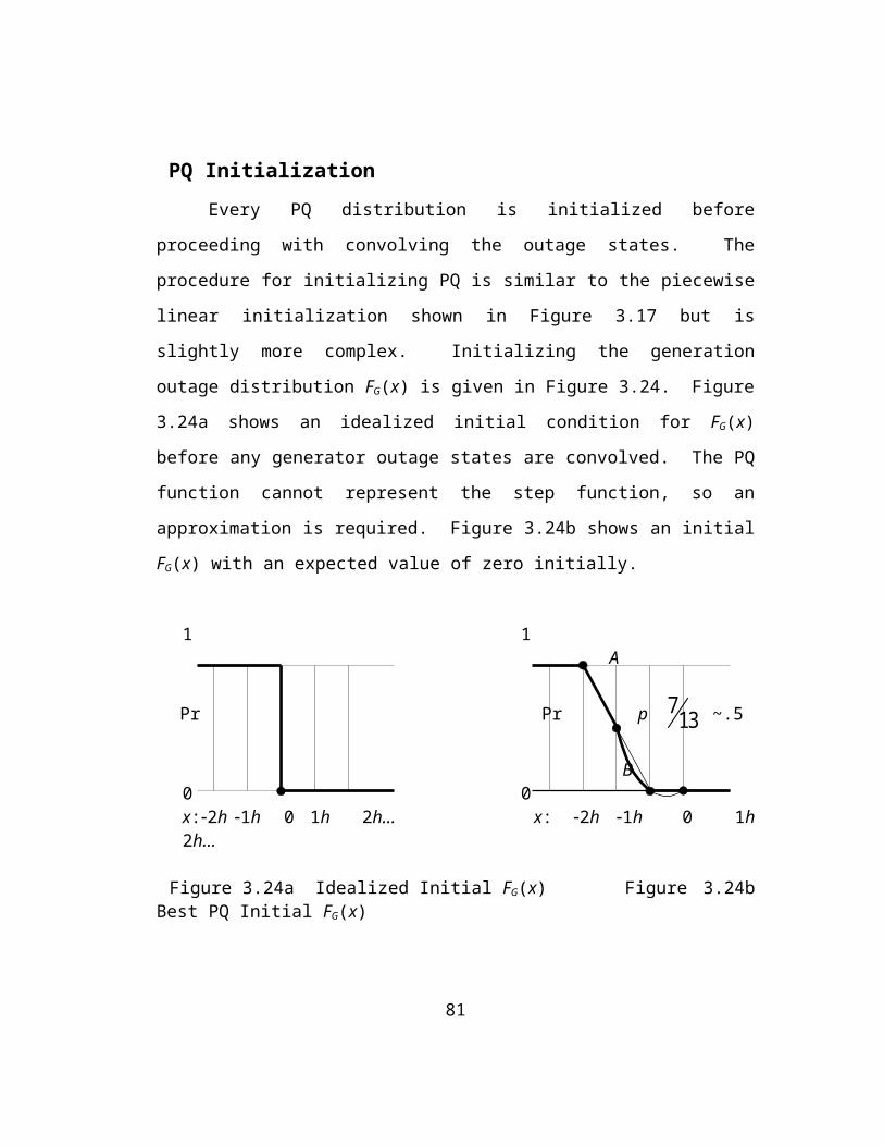
and the third curve near zero at the bottom. The error cannot be plotted on a log

scale because the error contains zero and negative values. An absolute value log plot

of the error does not appear to be meaningful.

Table 5.1 PQ Error Vs h MW Grid Increment and Vs x MW Outaged

OutagedCapacity

FE(x) Exacth=1 MW

FG(x) 720 incr.h=29.0985

FG(x) 360 incr.h=58.197

FG(x) 180 incr.h=116.394

10% .5400181pu error :

.5400144-.0000068

.5399837-.0000637

.5396498-.0006820

20% 1.708469E-3pu error :

1.708888E-3.0002452

1.710651E-3.0012771

1.722557E-3.0082460

30% 1.069758E-8pu error :

1.071004E-8.0011647

1.077244E-8.0069978

1.125576E-8.0521784

The listing in Table 5.1 has been created to show the wide variation in error

as h is doubled and halved. The dots in Figures 5.1a, 5.1b, and 5.2 are from the data

listed in Table 5.1 and are shown for ease in cross referencing this table to the other

figures. The error data in Table 5.1 is plotted in Figure 5.3 as a function of the h grid

increment size for x = 20% and 30%. The change in error with respect to h is very

nearly a cubic function of h. This allows very low errors to be achieved with PQ for

finite values of h. The PL interpolation error is plotted and is much greater [34].

91

0

0.01

0.02

0.03

0.04

0.05

0.06

0 20 40 60 80 100 120h grid spacing in MW for the ERCOT 286 generator problem

per u

nit e

rror

Figure 5.3 PQ Error - A Cubic Function Of h MW Grid Spacing

Load Model Representation Using FG(x)FG(x) is the probability outaged generation will exceed an x amount of MW.

Since the MaxGen configuration load MW is set equal to the total generation MW,

the amount of unserved MaxGen load is identically equal to the x amount of

generation randomly outaged. Reversing the x axis of FG(x) shows more clearly in

Figure 5.4 the amount of load that can be served and the load that cannot be served as

a function of FG(x).

Load Served FG(x)

Load Not Served

0 MW MW Load MaxGen MWFigure 5.4 Load Served (Not Served) By Random Generation

92

expected values are equal

FG(x)+ T(x)

For other load levels below the MaxGen configuration load, the area under

the tail of the FG(x) function gives the amount of energy not served, which is the

EUE. Figure 5.5 shows the load not served for a load level of y MW.

FG(x)

EUE = Load Not Served x

load y=0 increasing x increasing y y genr x=0

x + y =Ck

k

Ng

1

Figure 5.5 Load y Not Served By Random Generation Outages

The best indicator of reliability is the expected unserved energy, or rather the

EUE(x) as a function of the load y MW. In Figure 5.5, the EUE(x) is the integral of

FG(x) from x to ¥ or the EUE(y) is the integral from 0 to y. Note that this is the same

FG(x) function, only the x and y axes are reversed. The EUE is used to cover a one

hour period in this dissertation. Frequently the EUE is calculated for an entire year,

which includes all the operational data such as generator and line maintenance

schedules and hourly loads, but the transmission system reliability is best measured at

the highest load level in which there is no scheduled maintenance. Limiting the

analysis to peak load periods simplifies the data gathering process and allows the user

to study the primary problem rather than be burdened by less important data.

Therefore, the author has elected to calculate the transmission system reliability and

the transmission system’s effect on generation reliability only at the peak load

periods.

93

3

stat

e

gen

erat

ors

mo

dele

d as

2

stat

e

gen

erat

ors 3 state generators modeled as 3 state generators

FG(x) is the distribution function describing the generation availability for the

total system. This single area FG(x) definition of generator supply reliability is

extended to mean the relative generation reliability at every load bus in the network.

This is a physical interpretation of the system, in which the network is constrained by

the total generation supply and its randomness of outages and by the ability of the

transmission system to deliver power. Loss of load due to generation outages is to be

shared proportionately on all load buses in this model. Another way of stating this is

to say that every bus has the same electrical network opportunity of receiving power

if no transmission constraints exist. This definition is called load-loss-sharing and its

use allows a straightforward approach to solving the composite generation-

transmission reliability problem. The LLS methodology was described in Chapter 3.

The LLS approach provides a framework for uniquely defining bus loads

under generation outage conditions. The LLS simply calls for a uniform and

proportionate load reduction across the network to balance the total power

requirement when generation is outaged. Figure 5.6 is a picture attempting to convey

the idea that a simple linkage exists between generation and load. A reduction in

generation leads to a corresponding load shedding in the load flow. Applying the

load shedding uniformly across the network for all generator outage states produces a

load distribution very nearly the same as FG(x) with its x axis reversed. The

incremental changes in the network line flows can be calculated as all the generation

outages are occurring. Because the generation and load are scattered across the

network, the incremental line flow distributions that result are quite different from

the generation and load distributions. The probabilistic loading of the lines provides

a test of the ability of the transmission system to deliver the available generated

power.

94

Generation Transmission Load

generation states define max loads

generation load

Figure 5.6 Relationship Between Generation And Served Load

Other load models can be constructed in which the mathematical formulation

is too complex to be modeled using the convolution method. Chapter 4 described the

no-load-loss-sharing method as being one in which the convolution method is not

applicable. This is because the power from outaged generators cannot be directly

linked to specific load buses using NLLS. The NLLS solution itself is not unique.

For example, the NLLS method allows surplus generation to be used by load areas

needing capacity, but it fails to specify how the surplus capacity is to be allocated.

Numerical examples are given to illustrate the NLLS problems.

Three areas, A, B, C, have loads of 90, 100, and 110 MW respectively. Each

area has two 75 MW generators for a total network capacity of 450 MW. If area A

loses a generator then it will need 15 MW from one of the other areas. Which area?

The choice is arbitrary. An infinite number of possibilities exist in this example with

no load shedding. The solution is not unique.

Continuing with a second example: let area A lose two generators and area B

lose one generator. Area A needs 90 MW and area B needs 25 MW. Area C has 40

MW spare capacity but the allocation of this 40 MW to A and/or to B is not defined.

The split could be proportioned using ratios of unserved load to total unserved load,

or by area load to total load, or by capacity outaged to total capacity outaged, or by

order of occurrence of outaged generation, or by any other means the areas have

95

agreed to use. The selection of the proper NLLS methodology based on criteria such

as social, financial, and/or political objectives is clearly beyond the scope of this

dissertation. In this last example, the LLS method gives each area 75% (225/300) of

the total area requirement, which is 67.5, 75, and 82.5 MW respectively.

Solutions for the above examples have not yet been fully defined in the real

world. These kinds of load sheddings and generation allocations will soon be under

the control of an Independent System Operator in each region. The new operational

rules for the ISO are still under consideration at this time. Not knowing the specific

rules by which an NLLS methodology will operate eliminates the possibility of using

NLLS within the context of the convolution method in this dissertation.

The last item for discussion in this chapter is the lack of specifying a set of

loads in the PLF model. Two convolution approaches are commonly used. One way

is to start with an equivalent load duration curve (ELDC) [34] and then convolve

generation states into that load curve. This is the Booth-Baleriaux method [48] and is

widely used in production costing programs. Initially all the load under the ELDC is

unserved energy. Each generator convolved into the ELDC reduces the amount of

unserved load. The residual ELDC after all generators are convolved is used to

calculate the LOLP and EUE.

The second approach is to convolve all the generator states together to

develop either a capacity availability distribution or a capacity outage distribution.

The LOLP is found by looking up the probability of being able to serve the peak load

level. Likewise, the total unserved energy is calculated by summing all the one hour

EUE’s as calculated in Equation 3.17 for each hour. For production costing, the

ELDC method and the convolved generation states processes are equivalent, although

their computational speed may be slightly different.

However, in the composite G-T problem presented here, the ELDC approach

cannot be used for two reasons. First, the use of ELDC for a multi-area problem

corrupts the time coincidence of hourly load information. This will make the ELDC

96

approach give incorrect results. To overcome this problem in the GRIP program, a

set of weekly ELDC are used to regain some of the time coincidence. The method

selected in this dissertation only looks at the system during peak load conditions and

assumes that the network loads are in proportion to the generation capacity owned.

The second reason ELDC cannot be used is because there is no direct and

simple calculation procedure for calculating line flows in the network when a

generator is outaged (as in Figure 5.6). There may be a convolution procedure to

calculate the line flows when using ELDC loads, but it does not yet exist, and it will

probably be more complicated and harder to understand than this model.

A third, and softer, reason the ELDC approach is not desirable has to do with

the way transmission planners view the system. Transmission planning engineers are

interested in testing the transmission system under peak loading conditions because

this drives their recommendations for new system (capacity) improvements.

Therefore, the PLF model in this dissertation has been designed to accommodate

their viewpoint by testing the reliability of the generation and transmission systems

during peak load hours. The approach taken here allows the load level to be looked

up in a tabular form long after the computer runs are completed. Since the load level

is not part of the input data, the study results are not affected by how the load data

has been entered, thereby making the study results more robust and applicable over a

wider range of loads than a study that has been run for a specific set of loads.

97

Chapter 6Load Flow Solution

An AC1 load flow solution is used in the PLF model to solve the MaxGen

load flow and a load flow solution for each outaged generator. Each generator

outaged provides a means of calculating incremental real power flow in each line,

which is used to calculate the real line power distribution factors Hj,k [1,29,55].

The load flow is an electrical network solution used primarily by the electric

utility industry in which load power and generation power requirements are specified.

Additional operating constraints are also specified, such as generator reactive limits

and autotransformer tap range limits. Voltage is controlled by adjusting generator

reactive powers and by adjusting autotransformer taps. Slack and swing real power

generation is adjusted to meet real power requirements within each control area and

for the total system respectively. Since losses are nonlinear, an iterative solution

procedure is required in which successive corrections are made to the bus voltages.

These bus voltages are used to calculate transmission line and transformer power

flows that are compared with bus shunt requirements of load and generation. The

differences are real power DP and reactive power DQ mismatch at each bus. The

vector of power mismatches are used in a matrix solution to calculate small

corrections to the bus voltage angles VF and bus voltage magnitudes VM.

The Jacobian SolutionOne of the most popular solution techniques utilizes the Jacobian [J ] real

number matrix solution as shown in Equation 6.1 and in [68,69].

DD

DD

FPQ

J JJ J

VVM

×

11 12

21 22 (6.1)

1 AC means the network has complex line impedances, complex voltages, and complex loads.

98

Frequently the [J12] and [J21] matrices are omitted in the use of Equation 6.1.

This decouples the real and reactive power solutions. It also saves a considerable

amount of matrix fill that occurs in the sparse matrix solution when [J12] and [J21] are

present. This decoupling improves solution speed but leads to solution difficulties if

lines have high R/X ratios. The Jacobian sometimes has difficulty starting from a flat

start in which the voltages are far from the final solution. This may result in an early

voltage collapse or infeasible solution. The Jacobian solution may have a premature

voltage collapse in electrical networks that are difficult to control the voltage or are

operating near a maximum power transfer limit (MaxGen load flow conditions).

Another problem with the use of Equation 6.1 is the need to convert polar bus

voltages into rectangular bus voltages to calculate line currents. This is time

consuming computationally and adds some additional solution error. Load flow

solution error is critical in the PLF model because errors can be cumulative. The use

of real*4 voltages1 in Equation 6.1 will not work reliably here. Real*8 bus voltages1

are needed to achieve bus convergence tolerance of better than .01 MVA.

New Matrix SolutionWith these deficiencies in mind, a new load flow solution technique has been

designed that: 1) executes about as fast as the Jacobian computationally; 2) has much

better solution stability than the Jacobian; and 3) provides much better solution

accuracy. The new method simultaneously uses two interleaved sparse matrices to

better control real and reactive powers and their effects on incremental voltages. A

new form of bus voltage using three numbers instead of two allows both polar and

rectangular voltages to be represented at the same time without the use of

computationally inefficient trigonometric conversions. The new method of

representing the voltage at bus i is shown in Equation 6.2.

1 Single precision is real*4 with 7 decimal digits; double precision is real*8 with 16 decimal digits.

99

VMi ´VAi = VMi ÐVFi = VMi ´[cos(VFi) + j sin(VFi)] (6.2)

In Equation 6.2, real number angles VFi have been replaced with complex

number angles VAi. A necessary property of VAi is that its magnitude is always unity.

VAi contains the complete angle information as a complex number and is much faster

for a computer program to use in calculating line flows. VAi is the rectangular form

needed to calculate line flows. Angle additions in the new PLF matrix solution(s) are

performed as complex number multiplications.

An initial load flow solution begins with all voltages set to desired values of

per unit voltage. Regulated voltage buses are specified with voltages to be held

constant by adjusting transformer taps or generation reactive power. Unregulated

buses may be set at nominal initial values such as 1.00 per unit. The initial load

flow solution iteration should have only an angle calculation while holding bus

voltages constant. The power error is greatly reduced before introducing voltage

adjustments. This avoids the first iteration flat start Jacobian divergence problem.

[(DP, j0)] = [Y ]×[DV ] (6.3)

[VAi = VAi ´ (1.D0 + DVi ) / CDABS(1.D0 + DVi ) ] " i=1, Nb (6.4)

An approximation to the decoupled Jacobian equation [DP] = [J11]×[DVF] is

shown in Equation 6.3. [Y ] is an approximation to [J11]. Equations 6.3 and 6.4 are

used together to provide all the load flow bus power angle calculations. Real*4 [DVi]

and real*8 [VAi] are complex bus voltage vectors. [Y ] is an n×n real*4 complex

sparse nodal admittance matrix. 1.D0 is a FORTRAN1 double precision 1.0 number,

and CDABS is the FORTRAN routine for finding a complex double precision

absolute value number. [Y ] is composed only of complex R+jX transmission line

1 These FORTRAN statements must be constructed as shown or the 16 digit accuracy in the calculation will be rounded to 8 digits.

100

impedances in per unit1. [Y ] contains no shunt admittances except a single low

resistance (<10-10 pu ohms) at the system swing bus. [DP] is the vector of real

powers summed into each bus. The sparse matrix technique in [97] is used to solve

Equation 6.3. The solution using [97] has three steps: simulation; reduction

(factoring); and solution. The simulation and factoring of [Y ] is performed once.

The solution phase of Equation 6.3 is repeated with each load flow iteration using a

new set of [DP] to find a new set of [DV ]. The new DVi terms are used in Equation

6.4 to provide angle corrections to VAi.

Equation 6.4 shows FORTRAN1 double precision functions because they are

critical to the proper update of the bus VAi real*8 complex voltage angles. Here is a

brief explanation of how Equation 6.4 works. DVi is a very small (magnitude of 10-1

to 10-16) real*4 incremental complex voltage. The imaginary component of DVi

contains angle rotation information to be applied to VAi as shown in Figure 6.1.

imaginary DVi

DVAi real DVi

0 1

Figure 6.1 Imaginary DVi Converted To Angle DVAi

The FORTRAN real*8 double precision 1.D0 constant is added to DVi . This

is necessary to retain the original precision of DVi . An angle rotation vector is

created as shown in Figure 6.1. The delta angle vector is normalized in the operation

(1.D0 + DVi ) / CDABS(1.D0 + DVi ) and then multiplied times the unity real*8

complex angle VAi. The CDABS FORTRAN function is required in the denominator

in Equation 6.4 to retain the full 16 digit accuracy in the normalization of the 16 digit

1 All internal calculations are on a 1 MVA basis; one pu amp times one pu volt is one MVA.

101

rotation vector (1.D0+DVi). All the above statements are necessary to retain solution

precision.

The second step in the new load flow solution method is to perform a voltage

magnitude correction calculation. Equations 6.5 and 6.6 are used to correct the [VM].

[(DP, -jDQ)] = [Ys]×[DV ] (6.5)

[VMi = VMi + Real(DVi )] " i=1, Nb (6.6)

An approximation to the decoupled Jacobian equation [DQ] = [J22]×[DVM] is

shown in Equation 6.5. [Ys] is an approximation to [J22]. Equations 6.5 and 6.6 are

used together to provide the new voltage magnitude estimates on unregulated buses.

Real*4 Real(DVi) and real*8 real VMi are incremental magnitude and total magnitude

bus i voltages respectively1. [Ys] is an n×n real*4 complex sparse nodal admittance

matrix that is identical to [Y ] in every way except for the many shunt elements that

are added to [Ys]. [Ys] additional shunt admittances are:

· 2 ´ constant conductance of bus shunt MW,

· 2 ´ constant susceptance bus shunt MVAR, + capacitive, - inductive,

· 2 ´ half the total line charging susceptance in MVAR,

· autotransformer voltage regulated buses with shunts >1010 pu mhos, and

· generator voltage regulated buses with shunts >1010 pu mhos.

The 2 ´ factors arise from the derivative of the bus voltage squared terms on

the constant admittance shunt elements. For any bus i in the network with shunt

reactance Bi (+capacitive, -inductive), the reactive power Qi supplied by the shunt

reactance is Qi = Bi VMi2, (all variables are real numbers). The change in reactive

power through the B shunt admittance with respect to voltage magnitude is obtained

by taking the derivative so that DQi = 2Bi DVMi . The incremental voltage is related to

1 Note that [DP] and [DQ] are to always be recalculated as summations of all real and reactive flows into each bus before using either Equation 6.3 or 6.5 and that the sign of complex power is defined from P+jQ = VI*.

102

the incremental power as DVMi = [2Bi]-1DQi . Thus, the factor of 2 is needed to

provide the proper relationship between incremental voltage and reactive power.

The regulated buses are grounded through very small resistances (10-11 ohms)

to hold the regulated bus voltage changes to nearly zero volts when solving Equation

6.5. This provides a means of absolute control on the voltage regulated buses. In

order to reach a solution using Equations 6.3 through 6.6, other adjustments must be

made. Because autotransformer voltages are held rigidly fixed, the taps must be

adjusted with each iteration to account for reactive power mismatch on the regulated

bus. This is an external operation not affecting the matrices [Y ] and [Ys]. The same

is true for regulated generation buses in which the reactive power produced must be

adjusted to account for reactive power mismatch. In the course of iteratively solving

Equations 6.3 through 6.6, transformer taps may exceed their limits, and generator

reactive capability may exceed their reactive limits. When this happens the [Ys]

matrix may need to be reformulated ungrounding the regulated buses so that the

previously regulated buses are now unregulated and can seek their own voltages

levels. These previously regulated buses are unregulated because their regulating

devices fail to have enough range to control the bus voltages. Also during the

iterative process, real power sources and/or loads must be adjusted as slack

generation in each area to account for real power losses. Power correction at the

system swing bus is not necessary if every area’s slack generation is properly set.

Equation 6.5 gives excellent performance for voltage correction because it uses:

1) both real and reactive power mismatch, 2) both real and reactive line impedances in

their correct form as complex values, 3) both real and reactive shunt admittances in their

correct form as complex values, and 4) absolute control over the regulated bus voltages.

Frequently the data submitted by utility engineers have subtle errors. One

common error is the specification of individually regulating the voltage of two buses

connected by a very low impedance line. If this occurs, the load flow program

should respecify all regulating devices to control a single bus and let the others be

103

unregulated as shown in Table 6.1. Otherwise the solution may result in two voltage

controlling devices fighting each other. Additional computer code is usually required

to coordinate the tap changing of several autotransformers in parallel or

autotransformers trying to regulate the same buses as generators. There may be an

infinite number of possible solutions of reactive power settings and tap settings that

are all feasible, although there is usually a best solution based on other requirements.

Table 6.1 shows a typical load flow solution using Equations 6.3 through 6.6

for a 2231 bus ERCOT load flow test case. The computer runs show two regulated

buses reassigned to avoid a conflict in regulating the voltages of buses connected by

(almost) zero impedance lines. The maximum sparse matrix size is 10915 complex

numbers and after factoring the matrix using bi-factorization [97], the final matrix

size is 10047 complex numbers. The simulation and factoring process required only

two seconds on a pentium 75 MHz PC using [97].

The solution in Table 6.1 is a MaxGen configuration load flow run in which the

load is scaled upward to match the installed generation of 58197 MW. The printout

shows 147 power plant buses in the load flow, although 286 generators in the case can

have random outages. Many load flow buses have more than one generator. The load

flow solution starts with a flat start, and the Table 6.1 largest power mismatches

initially are 2271 MW at bus 1900 and 1139 MVAR at bus 4234.

104

Table 6.1 Example Of Load Flow Solution Convergence Using New Method

Load Flow Solution Monitor: Number of buses = 2231 5500 max Number of generators = 147 Number of circuits = 3092 6500 max Number of xformers = 553 1200 max Number of areas = 9 20 max Swing Bus = 4546 Read load flow data = 0h 0m 3s regulated bus 6235 reassigned to bus 6230 regulated bus 6444 reassigned to bus 6443 Matrix factoring time = 0h 0m 2s Matrix initial size = 10915 20000 max Matrix final size = 10047

************************************* * Generation is at maximum capacity * * Bus loads have been scaled upward * * Area interchanges have been reset * * Generator Qmn/mx is now unlimited * *************************************

load flow solution monitor ... iter 0 bus 1900 perr= 2271.01 bus 4234 qerr= 1138.74 0.11 sec iter 1 bus 5915 perr= 113.54 bus 4234 qerr= 854.87 0.33 sec iter 2 bus 1409 perr= 38.27 bus 4488 qerr= 39.49 0.27 sec iter 3 bus 1409 perr= 15.45 bus 8441 qerr= 13.70 0.22 sec iter 4 bus 1409 perr= 3.27 bus 1032 qerr= 3.43 0.22 sec iter 5 bus 8442 perr= 0.47 bus 8441 qerr= 1.89 0.33 sec iter 6 bus 8442 perr= 0.25 bus 4726 qerr= 0.61 0.27 sec iter 7 bus 8442 perr= 0.08 bus 4726 qerr= 0.27 0.27 sec iter 8 bus 8442 perr= 0.04 bus 4726 qerr= 0.12 0.22 sec iter 9 bus 6480 perr= 0.01 bus 4726 qerr= 0.05 0.33 sec iter 10 bus 6480 perr= 0.01 bus 4726 qerr= 0.02 0.22 sec iter 11 bus 4548 perr= 0.00 bus 4726 qerr= 0.01 0.27 sec iter 12 bus 4548 perr= 0.00 bus 4726 qerr= 0.00 0.22 sec

a load flow solution has been found iteration time = 3 sec total load flow time = 10 sec

105

FG(x)

The first iteration includes solving Equations 6.3 through 6.6 and the power

mismatches drop to 114 MW and 855 MVAR. The solution continues until both real

and reactive mismatches are less than .01 MW and .01 MVAR at all buses in the

network. The new matrix solution process is capable of solving this load flow down

to a tolerance of DP=1 Watt and DQ=1 VoltAmp, but this requires 31 iterations.

A popular commercial program used to perform ERCOT load flow studies

will sometimes fail to converge at the .1 MVA maximum bus mismatch level. This is

due to the representation of substation buses as short transmission lines at power

plants and major switching stations in the ERCOT system. The ERCOT engineers

need to be able to see the internal flows within substations to see if breakers and

switches have currents exceeding ratings. However, the extremely small voltage drop

across these very short lines is not captured properly by the single precision bus

voltages used in this commercial program.

In the example shown in Table 6.1 there is no matrix reformation because all

reactive and tap changing limits are ignored. A ‘normal’ load flow run representing a

seasonal load level will typically have one instance of matrix reformation and a total of

eight iterations. If the MaxGen configuration load flow shown here is run with the

voltage controlling constraints fully applied, low voltages will occur, and possibly

voltage collapse will occur. This MaxGen configuration load flow is a difficult case to

solve because the load level is far beyond what has been planned and insufficient reactive

power for voltage support may be a problem. The convolution requirements of linearity

and a MaxGen configuration load flow condition forces the acceptance of running this

case with voltage controlling device constraints eased. The fact that such a case does

converge shows that, if sufficient reactive capacity is installed in the real system, then it

could support the higher loads. Therefore, the additional reactive support assumption is a

reasonable simplifying assumption for the scope of this dissertation topic.

106

Chapter 7Line Distribution Factors

As each generator is outaged, the transmission line real power flows

throughout the network change. These incremental changes in power flows provide a

unique description of how power was being delivered from the generator to all the

loads before the generator was outaged. The purpose of this chapter is to show how

these incremental flows are converted into line distribution factors Hj,k [1,29,55],

how they are stored in the computer, and how they are linearly combined to predict

new incremental line flows not calculated explicitly by a load flow solution.

MethodologyThe MaxGen configuration load flow has all lines and generators in service,

and loads are at maximum levels possible. If a single generator fails to run, the

network load is reduced to match the remaining available generation. This will cause

an incremental change in transmission real power flows throughout the network.

Each generator individual failure will cause a set of incremental line real power flows

and a reduction in total system load and real losses equal to the generation amount

outaged.

Suppose two generators at the same load flow bus are outaged at the same

time. The network incremental real power line flows are nearly the same as the sum

of the individual incremental real power line flows from each generator being

outaged. They are the same if incremental losses are linear. Therefore, any two

generators outaged in the network anywhere create incremental line flows that are

nearly the sums of the individual incremental real power line flows caused by the two

outaged generators if incremental losses are linear.

107

If this process were truly linear, the sums of all the incremental flows of all

the generators could be used to sum all the incremental flows on all lines and the

MaxGen configuration base case real line flows will be created. It is not true, but it is

almost true. Table 7.1 shows the error differences between the actual MaxGen

configuration load flow line MW flows for 42 of the most heavily loaded lines and

the total MW line flows created by summing incremental flows for the 286 generator

ERCOT case. The incremental flows are summed as +flows and -flows, and these

are added to make the total MW column. The MW error compared to the actual

MaxGen configuration load flow is shown. The last column shows the percentage

the dominant + or - flows must be scaled to make the error go to zero.

Table 7.1 is a sample of the 3000+ lines in this case. The lines listed have

some of the highest MW loading in the MaxGen configuration load flow case. Lines

such as generator step-up transformers with flows in only one direction have been

omitted because they have almost zero error. The more interesting lines with flows

in both directions are listed in Table 7.1.

The last column of Table 7.1 is a set of scale factors. Each line has a unique

scale factor to make the sum of incremental flows equal the actual line flow. This

scale factor is only applied to the incremental flows in the dominant direction. The

dominant flow direction is the direction with the largest sum of incremental flows.

For example, the first line in Table 7.1 has a dominant flow of -1552.4 MW.

Applying the reduction of 0.8% to all negative incremental flows for this line reduces

the negative flow sum to -1540.0 MW. Then 737.1-1540.0 = -802.9, which is the

actual MW flow in the MaxGen configuration load flow case for this line.

108

Table 7.1 Summation Error And % Correction Of Incremental MW Flows LINE FROM TO (+FLOW) + (-FLOW) = TOTAL ACTUAL ERROR SCALE BUS BUS MW MW MW MW MW % 1391 3390 4401 737.1 -1552.4 -815.3 -802.9 -12.4 -0.8 1038 2398 2428 1214.7 -2016.5 -801.8 -802.2 0.4 0.0 3084 9073 9074 1449.3 -810.0 639.3 639.8 -0.5 0.0 1087 2437 2453 1030.2 -409.4 620.8 624.8 -4.0 0.4 822 1873 1890 272.9 -869.5 -594.3 596.6 -2.2 -0.3 2550 7040 7056 963.8 -1564.3 -600.5 -594.1 -6.4 -0.4 823 1873 1900 177.5 -757.4 581.3 -579.9 1.4 0.2 598 1436 1853 1183.7 -627.5 556.2 558.8 -2.5 0.2 853 1900 1902 1326.6 -784.1 542.5 558.6 -16.0 1.2 849 1890 1932 915.1 -366.9 548.2 552.7 -4.4 0.5 728 1690 2373 756.2 -205.6 550.6 547.8 2.8 -0.4 601 1436 1900 674.9 -1229.3 -554.4 -545.8 -8.7 -0.7 1046 2406 2420 672.4 -1213.2 -540.8 -541.8 1.0 0.1 742 1695 1697 713.4 -186.2 527.2 538.5 -11.3 1.6 1242 3100 3103 842.3 -309.6 532.7 533.1 -0.5 0.1 745 1695 2466 633.6 -115.9 517.7 526.1 -8.4 1.3 1045 2406 2407 877.1 -357.2 519.8 522.8 -2.8 0.3 1621 4112 4383 1519.6 -991.5 528.1 521.3 6.8 -0.4 1396 3391 4401 479.0 -971.6 -492.6 -498.2 5.6 0.6 1071 2428 4401 1312.2 -1813.1 -500.9 -496.7 -4.2 -0.2 1072 2428 4401 1312.2 -1813.1 -500.9 -496.7 -0.2 -4.2 1243 3100 3105 675.3 -181.7 493.6 496.7 -3.1 0.5 1666 4192 4714 738.8 -243.1 495.7 496.1 -0.4 0.1 1390 3390 3409 1568.7 -1055.5 513.2 495.8 17.4 -1.1 891 1930 1932 406.6 -896.3 -489.7 -495.7 6.0 0.7 1078 2432 2433 1809.1 -1304.0 505.1 492.3 12.8 -0.7 862 1907 1911 1115.0 -633.2 481.8 481.0 0.8 -0.1 1751 4356 4488 315.3 -784.3 -469.0 -474.0 4.9 0.6 1752 4356 4488 315.3 -784.3 -469.0 -474.0 4.9 0.6 1246 3100 3138 541.4 -69.2 472.2 473.7 -1.4 0.3 1420 3409 3414 2416.6 -1960.0 456.6 470.4 -13.8 0.6 584 1425 6100 521.7 -971.1 -449.4 -456.5 7.2 0.7 1820 4675 4676 499.4 -943.7 -444.3 -455.4 11.2 1.2 854 1902 1907 1242.0 -800.3 441.7 454.2 -12.5 1.0 744 1695 2461 567.3 -120.5 446.8 452.5 -5.7 1.0 1127 2461 2468 780.4 -341.1 439.3 449.3 -10.0 1.3 1070 2428 3123 559.7 -1010.1 -450.4 -445.8 -4.5 -0.5 1245 3100 3115 828.5 -386.3 442.2 443.0 -0.7 0.1 1622 4112 4470 1118.8 -673.9 444.9 441.4 3.4 -0.3 821 1873 1880 1232.3 -805.9 426.4 438.7 -12.3 1.0 868 1911 1913 1075.4 -639.7 435.7 435.4 0.2 0.0 1138 2466 2467 549.4 -119.1 430.3 434.1 -3.9 0.7Magnitude Averages: 5.7 MW 0.64%

109

The average of the absolute value of all scale factors for this 286 generator

system is 2.22%. Many of the larger scale factors are lines not carrying much power.

To better measure the overall error in terms of heavily loaded lines, the absolute

value of all scale factors was weighted according to real power flow with respect to

the sum of the absolute value of real power flows on all lines. The weighted error is

0.97% for a solution tolerance of .01 MW/MVAR. The system appears to be fairly

linear in power. The linear combination of incremental flows associated with

specific generators seems to be a feasible approach.

The solution tolerance was adjusted to see its effect on the average weighted

error. With a tolerance of 0.1 MW/MVAR the error is 0.98%, almost no change.

With a tolerance of 1.0 MW/MVAR the error is 1.19%. With a tolerance of 10

MW/MVAR, the average weighted error is 5.06%. This seems to indicate that a

tolerance of .01 MW/MVAR is not necessary. These averages are misleading

however. The cumulative error of adding the incremental flows from 286 load flow

cases is itself a random variable. A few lines might have a substantial error due to a

load flow solution error bias. To illustrate how this cumulative error could occur, let

a line l have a MaxGen configuration base case flow of P+d where P is the correct

solution and d is a small error. Let i = 1...Ng generators be outaged one at a time

with incremental flows Ii+(±r) in line l where ±r is assumed to be a uniformly

distributed random error in the solution of the incremental line l flow cases. The total

expected flow is the sum of the differences or (Ii+(±r)-P+d). The best we can

hope for is to have the ±r random errors sum to zero and drop out. If this is the case,

we are still left with a possibly large d×Ng error because the line flow sum is now Ii

-(P×Ng)+(d×Ng). The d error has been magnified Ng times due to the base case

error. If the ±r did not sum to zero as assumed, the error could be even larger,

depending on whether the ±r sum adds to or subtracts from to the d×Ng error. The

load flow solution errors must be reduced as much as possible.

In reviewing the sum of line flows from incremental generator outage flows

in the 286 generator case, only a few lines are observed to have cumulative solution 110

errors. Lines 2460 and 3002 have the maximum MW error on the 1.0 MW/MVAR

tolerance load flow solution. These are good candidates for illustrating the MW error

as a function of the load flow solution tolerance. Figure 7.1 shows the MW error for

these two lines in the 286 generator case as solution tolerance is adjusted.

0.001

0.01

0.1

1

10

100

0.001 0.002 0.005 0.01 0.02 0.05 0.1 0.2 0.5 1

Load Flow Solution Tolerance - MW/MVAR

Sum

of I

ncre

men

tal F

low

s Er

ror -

MW

Line 2460Line 3002

Figure 7.1 An Example of Load Flow Solution Error Versus Solution Tolerance

The dashed line in Figure 7.1 is a better description of the line 3002 error

versus solution tolerance. The dip in error is probably due to the accidental

cancellation of base case solution error and sum of incremental flows error. No other

lines were observed to have this dip to almost zero error. Most lines have an almost

flat MW error between .01 and 0.1 solution tolerances suggesting that possibly 0.1

MW/MVAR error is acceptable. The 1 MW/MVAR tolerance did produce a large

amount of error in many lines and is not recommended. The .001 MW/MVAR

solution tolerance did little to reduce error further from the .01 tolerance and is

probably not necessary. Since there is little difference in run time between .01 and

0.1 MW/MVAR solutions, there is little penalty in choosing the conservative solution

tolerance of .01 MW/MVAR for all load flow solutions. This improves linearity

111

which allows the sum of all incremental flows to be nearer to the MaxGen

configuration flows.

The process for calculating and storing all the incremental real power flows

will now be explained in more detail. The incremental power flows from individual

generators are used extensively in the process of solving for line flow probabilistic

distributions. Real generator incremental line flows and virtual generation

incremental flows are discussed along with the computer and solution requirements.

Real GeneratorsUsing the MaxGen configuration load flow as a reference case, each generator

is outaged one at a time. Each generator outaged load flow case is modified from the

MaxGen configuration case by removing the outaged generator from the case and

uniformly scaling down the bus loads across the network to account for the removed

generation capacity. In these special load flow solutions, 1) autotransformer taps are

held constant, 2) generator reactive is unlimited, 3) total network load is scaled

uniformly to act as the power slack generator, and 4) solution tolerance is held to .01

MW and .01 MVAR.

The purpose of outaging each generator is to develop a set of Hj,k power

distribution factors for all k=1...Ng generators and all j=1...N t transmission lines.

These are the per unit change in power flow in each line j as a result of loss of

generator k. Any single Hj,k factor is calculated by subtracting the outaged generator

k MW flow on line j from the corresponding MW flow in the MaxGen configuration

load flow and dividing that difference by Ck . This is repeated for all lines j for each

generator k.

Because the total size of Hj,k is large1, the j=1...N t line flows are written to

disk storage as they are created for each new generator k. The disk file these factors

1 The 286 generator case in Appendix B uses about 4 Mb of disk space to store all the Hj,k factors.

112

are written to is a random access binary file called H. Each record k in file H

corresponds to generator k. If H is viewed as a matrix, the rows are individual

generators, and the columns are individual transmission lines.

Once all line distribution factors have been calculated and stored in H, these

factors need to be adjusted so that the sums of all incremental flows on each line will

sum to the MaxGen configuration line flows. However, before the adjustment can

begin, a new file called HT is created, which is the transpose of H. Since the PLF

program will be accessing the Hj,k factors on a line by line basis, the random access

file needs to be accessible on the same basis. The HT rows are line data and the

columns are generators. Reading record j from HT gives immediate access to all the

distribution factors for line j. Without the HT file, the PLF computer run time could

be increased by several hours.

As each record of HT is read, incremental flows are partitioned into positive

and negative sets for each line where positive is arbitrarily one direction for the line

and negative is the opposite direction. The sum of all incremental flows on each line

will not sum exactly to produce the MaxGen configuration real power line flows. For

each line, the directional incremental flows in the direction that is dominant are

scaled by a real number multiplier so the sum of all flows will exactly yield the

MaxGen configuration flows on each line. The adjusted distributions are written

back to HT.

An example of this scaling process is shown in Table 7.1. Experience shows

that the scaling corrections are small for lines that are heavily loaded, about one

percent weighted average for the 286 generator system and about one percent for the

IEEE Reliability Test System [30].

113

Virtual GeneratorsThe real generation model described up to this point can only be used to shed

load for the entire system. However, load shedding across the total system does not

make sense as a corrective action. Selective load shedding of specific areas or even

specific buses associated with specific generators will be required to efficiently

unload the overloaded lines. Virtual generators are power injections into selected load

buses to effectively reduce load at these buses. The distribution factors [1] for the

virtual generators are calculated in the same manner as previously described for real

generators and are included in the set of Hj,k. Figure 7.2 shows how a group of three

buses have been selected to be candidates for load shedding. The ‘virtual generation’

injected in this example has been arbitrarily set at half the load of each bus.

virtual generator

load

incremental flows to all buses in the network

Figure 7.2 Virtual Generation Injected At Three Load Buses

114

In setting up the virtual generation incremental load flow, each virtual

generator k is made proportional to the real load on each bus in which load shedding

is to be executed proportionately (later) on all the load buses selected. The case is

solved, the incremental line flows are calculated, and then the flows are normalized.

These incremental line distribution factors are appended to the bottom of HT.

As in the real generator outage solutions, 1) autotransformer taps are held

constant, 2) generator reactive is unlimited, and 3) total network load is scaled

uniformly to act as the power slack generator. The solution tolerance can be relaxed.

Note that in the load flow solution, the virtual generation injection at a bus is one

thing, but the MaxGen configuration total system MW load being adjusted as slack

generation is quite another thing. They are handled separately as the load flow is

being solved. This means that the virtual generation injections are to be held

constant, while at the same time, the loads are being scaled upward or downward on

all load buses to meet the total load flow power requirement.

Note that no scaling is performed for the virtual generation distribution line

factors. There is no reference load flow case for checking the sums of incremental

virtual flows. So this process is skipped for the virtual distributions.

The selection of buses to be grouped together for proportional load shedding

is somewhat arbitrary, although the selection will affect the final output report

results. The author has elected to use the load areas originally defined in the load

flow data as the load shedding areas also. Another possibility, not yet modeled in the

PLF program, is to let every bus in the load flow be a separate candidate for load

shedding. This highest degree of detail in the load shedding model would allow the

LOLP and EUE of every bus in the network to be calculated as a function of both the

generation system and transmission system reliability. This information is of great

value, so the PLF program will be programmed in the future to model individual bus

load sheddings.

Real And Virtual Generation Superposition 115

Because the network is almost linear in real power, the incremental real power

flows of real and virtual generation can be linearly combined to produce a set of

incremental real power line flows that are representative of the incremental flows that

will occur if the specific AC load flow case of generation-to-load is set up and

solved. This superposition is only used in the load shedding operation explained in

Chapter 10. Figure 7.3 illustrates what happens when the virtual generation

distribution factors [1] are subtracted from the real generation distribution factors.

generation load generation load

Figure 7.3 Combined Real And Virtual Generation

Equation 7.1 shows how linear combinations of normalized Hj,k factors are

used to produce new generation-to-load factors Hj,m-n. For line j, the m terms are real

generators, and the n terms are virtual generators.

[ Hj,m-n = Hj,m - Hj,n ] " j =1, N t (7.1)

The process of linearly combining incremental flows from generators and

loads is consistent with the LLS methodology because all dispatches are to the total

system loads. This is an inherent part of the LLS method but not the NLLS method.

When the H distributions of generation and virtual generation are subtracted,

as they are in Equation 7.1 and in Figure 7.3, only the net incremental flows from

116

generation to load remain. This superposition principle has been tested analytically

in small three and four bus examples and is found to have a good theoretical basis.

Equation 7.1 was a very important development in the theory needed for the

PLF model. When (7.1) was implemented, it solved a major problem that was

impeding the successful implementation of the convolution methodology. Consider

this worst case situation as an example of the problem. Suppose a system has 300

generators, 2000 buses, and 3000 lines. Let one load flow require one second

solution time. The line distribution factors for all single generator outages to total

system load is 300´3000´4 = 3,600,000 bytes of storage and requires 300 seconds

of solution time. Now the problem of defining network incremental line flows for

specific load sheddings must be solved. Without using virtual generation and

Equation 7.1, the distribution factors for all combinations of load and generation is

calculated as 300´2000´3000´4 = 7,200,000,000 bytes and requires 300´2000 =

600,000 seconds or 167 hours of computer run time for just one study case! Clearly

this is not feasible. Using virtual generation and Equation 7.1, this drops to a total

storage requirement of (300+2000)´3000´4 = 27,600,000 bytes and 300+2000 =

2300 seconds or 40 minutes of computer run time, which is reasonable.

In setting up the 286 generator example case, the load (shedding) areas have

been defined according to the original load flow data with eight areas plus one new

area1. This is only nine load areas. All the load sheddings to remove transmission

limitations are done by scaling load proportionately within an area. Only nine virtual

generation cases are run and stored in the generator-line distribution file rather than

the 2000+ buses given as an example in the above discussion. This rather coarse

model of load shedding creates another problem. Some overloaded lines internal to

an area that are not strongly associated with the flows from generation, but are mostly

local load driven, cannot be unloaded with such a coarse load model. There is a way

1 The City of Austin has been split into two areas making the total ERCOT system nine load areas.

117

to get around this problem without needing to run virtual generation on every bus in

the system. This shortcut is described in Chapter 10 and allows the use of only major

load areas as virtual generation. This saves considerably on storage and run time but

produces less accurate results.

118

Chapter 8Probabilistic Line Flows

This chapter explains how the incremental line flows on each line due to each

generator being outaged are convolved together to form line flow distributions that

are cumulative and monotone decreasing. These distributions contain the generation

outage states information as well as how the power is redistributed throughout the

network as generators randomly fail.

By performing all convolutions before load sheddings, the generator outage

events are independent events and can be convolved in any order. If line flow

corrective actions were to be taken as the generators are convolved in calculating the

line flow distributions, then their outcomes become dependent, and the convolution

process would produce incorrect results. Load sheddings are performed as a last step

in the PLF model to maintain independence and linearity during the calculation of

line distributions.

The process for creating line flow distributions F±j(x) is similar to the process

for creating the generation function FG(x). Very briefly, the first step is to give all

lines a probability of one with flow equal to the MaxGen configuration MW flow.

Figure 8.1 shows how the line distribution functions are initialized for the MaxGen

configuration. Then the incremental line flows for all generator outages are

convolved one at a time recursively into the line distributions to produce a set of

probabilistic line flows.

Convolution Process MethodologyThe outcome of the complete set of all combinations of generation failure

states is described by FG(x). Because the generator outages are independent, the

generators can be convolved in any order without affecting the outcome of FG(x).

119

Each load bus and each load area receives a proportion of FG(x). Every specific

outage configuration has a specific set of line flows in the network. The MaxGen

configuration load flow and all the individual generator outage load flow cases are

explicitly enumerated and saved. These cases have little error in line flow

calculations1.

The network real power flows in transmission lines for two and more

generators simultaneously outaged is constructed by taking linear combinations of

incremental line flows from the individual generators outaged cases results. The

linear combination of all generators outaged simultaneously produces exactly zero

MW line flows everywhere, giving assurance that the linear combination of flows can

be very deep indeed without resulting in large solution errors.

Consider the flows on a single transmission line l, in the network. Every

combination of outaged generators has a probability. Linearly summing all the line l

incremental flows of the outaged generator cases and subtracting this sum from the

line l MaxGen configuration flow produces a specific MW flow for line l for this set

of generators outaged. All configurations of multiple generators being outaged

produces a corresponding set of line flows for line l. Using PQ convolution, the

linear combination of all these configurations can be efficiently calculated.

Calculating Line Probabilistic DistributionsThe Hj,k factors link the generator k states in Table 3.3 with the transmission

line j flows in Fj(x). Fj(x) = Pr[cj line flows > x] is similar to FG(x) except the range

of Fj(x) has both negative and positive x, whereas for the range of FG(x), x is 0

through Ck. Fj(x) is initialized to represent the MaxGen configuration flow xoj on

line j with probability of one as shown in Figure 8.1.

i-1 i i+1 i-1 i i+1

1 Small differences in results are seen in the order of convolving generators due to numerical machine roundoff errors and due to the PQ process itself not being an exact process.

120

1 1 A

MaxGen MW flow xoj p xoj

Pr r Pr

B0 0

hj PQ F±j(x) grid i steps hj PQ F±j(x) grid i steps

Figure 8.1a Idealized Initial F±j(x) Figure 8.1b Actual PQ Initial F±j(x)

Initially all generators are up and available and this produces the initial line

flow xoj in line j in the MaxGen configuration load flow. Outaging a generator k

produces an incremental change in flow of -Hj,k×Ck MW or -Hj,k×Dk MW if the

outage is partial in line j. For any line j, the set of generator states in Table 3.3

combined with Hj,k distribution factors defines the probabilistic line flows Fj(x) as

shown in Equation 8.1. Equation 8.1 is the total PQ convolution process for all lines

j, from 1 through N t.

[Fj(x) = [ (-Hj,k×Gk)·Fj(x) ] k = 1, Ng ] j = 1, N t (8.1)

In the MaxGen configuration, all the line flows due to all the generators on

line are already included and sum to xoj for each line j as shown in Equation 8.2. xoj

is also the base case MaxGen configuration line flow for line j. Equations 8.2

through 8.7 produce the same initialization of the line distribution shown Figure 8.1.

xoj = H Cj k

k

Ng

k,

×

1 (8.2)

121

Fj(x) is initialized for the MaxGen configuration as a real number real*4 precision

array

Fj(x < (i-b)hj) = 1 , (the array points < i)

Fj(x = (i-b)hj) = p ,(the array point =i), (8.3)

Fj(x > (i-b)hj) = 0 , (the array points > i)

where i is the discrete array integer point closest to xoj according to

i = INT(xh

oj

j+ b + .5) . (8.4)

The +.5 term in Equation 8.4 shifts the integer process range so that an i is found

allowing the xoj to fall within the r range of -.5 £ r<+.5 as shown in Figure 8.2.

1

0r: -1 -.5 0 +.5 +1

Figure 8.2 Initial Line Distribution Parameter p(r)

The hj MW grid spacing in Equation 8.4 is

hj = (xmaxj - xminj)/(number of grid increments) (8.5)

where xmaxj and xminj are the minimum and maximum values of line flow x that can

occur.

122

dots are common points referenced in Table 5.1 and Figures 5.1 and 5.2

3

sta

te

ge

ne

rat

or

s

m

od

el

ed

as

2

sta

te

ge

ne

rat

or

s 3 state generators modeled as 3 state generators

The xmaxj and xminj are calculated using

xmaxj = H Cj k k

k

Ng

, ×

1

for Hj,k > 0

xminj = H Cj k k

k

Ng

, ×

1

for Hj,k < 0 . (8.6)

Then p = (xh

oj

j+ b + .5) - i (8.7)

in which b is a shifter on the x axis to keep xmaxj and xminj within the range of the

discrete computer program array. For example, the discrete array Fj(x) may be

dimensioned from 1 through 360 (as is the PLF program). A mapping is needed

between the x MW line flows and the array positions. A simple linear conversion of

the form i=mx+b is appropriate in which the i are integer positions 1 through 360 in

the computer program array. Let 1 = m(xminj) +b and 360 = m(xmaxj) +b. Then

m = (360 - 1)/(xmaxj - xminj) = 1h j

, (8.8)

and b = 1 - xh j

min j , (8.9)

in which m and b allow the xminj and xmaxj to align exactly with the array end points.

Equation 8.1 will only produce low error on the lower right hand tail of Fj(x).

In order to model negative flow line overloads accurately, the line direction is

reversed and Equations 8.1- 8.9 repeated. This means that line j can have a second

Fj(x) in which the line flows have been reversed and the line overload is in the

negative flow direction. The -j in F-j(x) is used to signify convolution Fj(x) with

flows reversed for line j. Figures 8.1a and 8.1b show the forward and reversed line

flow functions Fj(x) and F-j(x) for line 1389 as an example. The log scale allows the

extremely small probabilities to be displayed.

123

1E-801E-751E-701E-651E-601E-551E-501E-451E-401E-351E-301E-251E-201E-151E-101E-05

1

-259

3-2

455

-231

7-2

178

-204

0-1

902

-176

4-1

625

-148

7-1

349

-121

1-1

073

-934

-796

-658

-520

-382

-243

-105 33 171

310

448

586

724

862

1001

1139

1277

1415

1553

1692

1830

1968

2106

2245

Line Flow - MW

Prob

abili

ty

Figure 8.1a Line 1389 Probabilistic Loading In The Forward Direction

1E-801E-751E-701E-651E-601E-551E-501E-451E-401E-351E-301E-251E-201E-151E-101E-05

1

-236

9-2

231

-209

2-1

954

-181

6-1

678

-154

0-1

401

-126

3-1

125

-987

-849

-710

-572

-434

-296

-157 -19

119

257

395

534

672

810

948

1086

1225

1363

1501

1639

1778

1916

2054

2192

2330

2469

Line Flow - MW

Prob

abili

ty

Figure 8.1b Line 1389 Probabilistic Loading In The Reverse Direction

124

PL

Line 1389 is centrally located in Texas and is probabilistically overloaded by

deficiencies in generation in either North Texas or deficiencies in generation in South

Texas. The maximum overloads are 242% forward and 221% reversed. However,

the probability the transmission line will ever actually be overloaded is extremely

small. The heavy horizontal line shows the line’s normal loading range of -1072 to

1072 MW. These curves are typical of all the probabilistic line loadings in this large

network. The xmaxj and xminj line extreme flows are usually large but the

probabilities of overload are extremely small. These extremely small probabilities

are easily calculated and observed using the convolution method. The enumeration

methods are not capable of examining this part of the probability space.

Screening and Ranking LinesA screening criteria is useful in deciding which lines to not monitor. For each

enumerated configuration with line outages as well as the configuration with all lines

in service, lines with xmaxj < Rj and xminj > -Rj are discarded from further analysis

since no generation failure states causing an overload on line j exist. This test is

performed before the line flow convolutions.

Lines with small Fj(x = Rj) < 10-12 can also be discarded. Experience shows

that lines with these very small probabilities of overload will not contribute any

observable amount of EUE to the final output results. For example, a line overloaded

by 1000 MW, at a probability of 10-12 for one hour, represents an energy of overload

of only .001 Watt! Obviously, this overload will contribute little to the overall EUE.

Experience with the ERCOT system has indicated that this screening process

results in about 500 lines out of a total of 3200 lines will be retained for probabilistic

overloading and load shedding analysis. This number is very system dependent and

will probably vary considerably for different systems. Only the ERCOT system has

been tested at this time.

125

Chapter 9Line Outage Model

This chapter presents a new method for modeling multiple simultaneous line

outages in large electric networks. The method: 1) calculates line currents and

powers; 2) tests for system separation; and 3) updates real power line distribution

factors [29,55] useful in linear programming (in Chapter 12) and probabilistic

models. A one-time factored sparse complex admittance matrix of the network series

line impedances is used to calculate incremental voltages from complex injection

currents. Each set of lines out of service requires one direct calculation. Differences

in solution results between this method and load flow for several lines and generators

outaged are shown in Chapter 11.

Dr. Ray Shoults at the University of Texas at Arlington developed the fast

line outage technique as a part of his dissertation [94]. An earlier method by Brown

[95] is similar to Shoults’ ‘zipflow’, but Brown’s method has more computational

error due to the sparse matrix structure and the way he stores and calculates

incremental voltages. Unfortunately, Dr. Shoults’ efficient computational method

was never properly published in a journal. This dissertation not only uses [94], but

shows how the zipflow theory in [94] can be extended to cover the case of many lines

outaged simultaneously. A paper has been submitted to the IEEE on this topic [55].

A second extension to [94] shows how new Hj,k factors can be estimated for

multiple lines outaged without actually running the load flows to calculate the new

distribution factors [55] for the new networks. These new methods are very efficient

computationally, which allows a greater number of line outage configurations to be

enumerated in conjunction with the total generation outage probability space.

126

Single Line OutagedA fast line removal approximation is used to avoid solving a new network

matrix with each line outage [94,95]. The use of a complex number matrix in this

zipflow formulation gives better results than a real number matrix of power and

voltage angle. The line removal involves a series of mathematical steps. Figure 9.1

shows the first step is the injection of (1Ð0) amp in and out of the line j to be

removed. This creates a set of small [DV] j ‘test’ voltages throughout the network.

The incremental voltages created on the ‘from bus’ and the ‘to bus’ ends of line j are

DVf j and DVt j respectively. Line j incremental current will be less than 1 amp if the 1

amp injected current circulates throughout the network.

DVf j Line j DVtj

‘from bus’ +1Ð0 amp -1Ð0 amp ‘to bus’

Figure 9.1 Inject 1 Amp In And Out Of Line j

Figure 9.2 shows the incremental line j current (DVf j -DVt j)Yj being scaled by a

complex number Sj in order to create a circulation current that is completely self

contained as a loop current within line j. This current includes the original base case

load flow current as well as the portion of the injected current flowing in line j. Line

j base case current is not canceled by this process. The purpose is to self-contain the

base case current within the local circulation current set up by Sj so that no line

currents from other adjacent lines from either the base case or from the injected

currents flow across the gaps shown in Figure 9.2. In practice, the line is not

removed from the matrix solution, but the equivalent voltages in the network are the

same as though line j has been removed.

127

Sj×DVf j Sj×DVtj

Sj = Ib j+[Sj×(DVf j -DVt j)×Yj]

from +Sj amp -Sj to

Figure 9.2 Single Line Removal Using Sj Injection Current

The mathematical steps to calculate Sj are outlined below. Begin the process

by solving a load flow of the network giving the set of all [V]b=[...Vf b j ...Vt b j ...]T.

Calculate the base case complex current Ib j of line j to be removed. The calculation

of Ib j should not include shunt elements to ground such as line charging. Including

shunt elements and currents in this line outage process increases solution error when

benchmarked against the same line outages solved with a full load flow solution.

Next, choose a single point on every line to measure line current. The PLF

model calculates base case and incremental line currents on the ‘to’ end of every line

because the PLF load flow autotransformer model has only a series Z with no shunt

element connected to the ‘to’ bus. This allows the autotransformer tap to not have a

shunt in the [Y] matrix. The importance of this choice is described below.

The [Y] complex nodal admittance matrix of the network is constructed from

real and reactive in-line series impedances. One bus in the network is grounded using

a low impedance shunt element and remains at zero incremental volts at all times.

Although any bus may be the grounded bus, it should be one that can regulate the

voltage under severe line outage conditions in a full AC load flow. The use of other

shunt elements in [Y] allows localized loop currents to flow to ground and reduces

the magnitude of incremental voltages remote from the outaged line j. The use of [Y]

without shunts (except the reference grounded bus) produces more accurate line

128

outage results than when shunts are included based on the author’s experience with

the model. The addition of shunts destroys the model’s ability to keep the

incremental line currents completely contained within the transmission lines

themselves. This means that the system separation test will be incorrect if shunts are

included. Also, the incremental line currents are used to calculate incremental line

powers. Shunts effectively drain away the small currents on remote lines from the

initial 1 amp injection. The model with shunts added will produce incremental

powers on remote lines that are too small when compared with a full AC load flow.

The next step is to find the set of all [DV] j. DVf j and DVt j are incremental

voltages resulting from the injection of ±1Ð0 amp into line j as shown in Figure 9.1.

Equation 9.1 shows this is a standard nodal admittance matrix solution. The PLF

model uses the sparse matrix technique in [97] to efficiently solve Equation 9.1.

[DV] j = [...DVf j ...DVt j ...]T = [Y]-1[...1...-1...]T (9.1)

The [DV] j calculated from the ±1Ð0 amp injections for line j are saved for

use in other calculations such as the outaging of many lines. The complex scale

factor Sj for scaling the incremental network bus voltages is given in Equation 9.2.

S IV V Y

jb j

f j t j j

- -

1 ( )D D (9.2)

Sj is also the complex injection current that produces the totally self contained

current in line j as shown in Figure 9.2. If less than .001 per unit amps injection

current flows through the rest of the network, there effectively are no alternative

paths for the injected current to flow other than the outaged line j. Then, the network

will be broken into two islands by the outage of line j if Equation 9.3 is true.

1 001- - £( ) .D DV V Yf j t j j

(9.3)129

Equation 9.4 creates a temporary [V]new set of voltages for the outage of line j.

[V]new = [V]b + Sj ×[DV] j (9.4)

Line currents including line shunt currents are calculated using [V]new to

check for line overloads with line j outaged. This process is repeated for all single

lines outaged and all [DV] j are saved for use in other calculations.

Multiple Lines OutagedMultiple line removal is an extension of single line removal in which complex

scalar Sj becomes complex vector [S] for n lines outaged simultaneously. Sj elements

of [S] are injection currents into and out of each of the lines j=1...n. An example for

n = 3 is shown in Figure 9.3.

from S1 = Ib1 + DI11S1 + DI12S2 + DI13S3 to

Line 1

S2 = Ib2 + DI21S1 + DI22S2 + DI23S3

Line 2

S3 = Ib3 + DI31S1 + DI32S2 + DI33S3

Line 3

Figure 9.3 Three Lines Outaged Example

130

In Figure Ib1, Ib2, Ib3 are the base case line complex currents for lines 1, 2, and

3, respectively. DI11, DI22, DI33 are the line self currents from the ±1Ð0 amp

injections on each individual line. DI12, DI13, DI21, DI23, DI31, and DI32 are the line

transfer coupling currents from the ±1Ð0 amp injections. For example, DI12 is the

current in line 1 from the ±1Ð0 amp injection in line 2. Incremental DIij currents on

lines i for injections j are calculated as shown in Equation 9.5 from the set of [DV]j

calculated in using Equation 9.1.

DIi j = (DVf ij - DVt ij) Yi (9.5)

Rearranging the equations shown in Figure 3 for n = 3 produces the matrix

Equation 9.6 for finding the complex [S] vector.

11

1

11 12 13

21 22 23

31 32 33

1

2

3

1

2

3

- - -- - -- - -

D D DD D DD D D

I I II I II I I

SSS

III

b

b

b

(9.6)

[S] complex scale factors (bus injection currents) simultaneously disconnect

all n lines from the network. Equation 9.6 is solved using Gauss elimination since

the matrix is dense and small. A singularity of Equation 9.6 indicates a system

separation. Any diagonal term becoming nearly zero during the solution of Equation

9.6 means the system has electrically isolated buses or system separation condition1.

What to do with the islands created by system separation is discussed at the end of

this chapter. After Equation 9.6 is solved, the new bus voltages [V]new for the case of

multiple n lines simultaneously outaged can be calculated using Equation 9.7.

[V]new = [V]b + j

n

1 Sj ×[DV] j (9.7)

1 The matrix will only become singular in the process of solving (9.6) if the network is broken up into islands by the removal of the lines being outaged.

131

Line currents including line shunt currents are calculated using [V]new to

check for line overloads with lines j=1...n outaged. The processes in Equations 9.5

through 9.7 are repeated for other sets of line outages.

Creating New H Factors For Line Outage CasesThis chapter has thus far presented models based on linear summations of

complex incremental line currents. However, complex incremental currents are not

directly usable in linear programming and probabilistic models based on the use of

real numbers. The real power distribution factors Hi,k are the set of per unit

incremental real powers in all lines i due to all generators k. The Hi,k factors have

been calculated using incremental load flow solutions. Next in this chapter, a method

for updating the Hi,k factors is presented. The updated H represents real power

distributions for multiple line outages. They are estimated without running new AC

incremental load flow cases for each line outage configuration.

Real Power Matrix Approach Fails:

A line outage model was developed using all real powers in a matrix similar

to Equation 9.6 for multiple lines outaged in order to calculate a set of real [S] scale

factors. The real power model worked well in predicting incremental line powers for

single line outages. It frequently failed to predict system separation because the real

matrix was not singular enough when the system was in a state of separation. It

performed poorly for multiple line outages in predicting real power flow

distributions. Subsequently, the approach using only a real power matrix to model

line outages was abandoned.

Real Powers From Complex Currents Approach Succeeds:

132

The successful solution approach is to perform all line outages using only

Equation 9.1 through 9.7, which contain only complex incremental currents and

voltages. Real incremental powers are calculated as a secondary operation from the

complex incremental currents in the line outage model.

Each generator k has a set of Hi,k real power per unit distribution factors for

all lines i. For any line or lines outaged, each set of power distribution factors for

each generator is updated as a separate operation for each generator. These updated

factors are calculated, used immediately, and then disposed of because far too many

configurations exist to store all of them in computer files or memory. The updating

process presented here is very computationally efficient and is much faster than

running successive load flows to generate new distribution factors.

Assume line j is to be outaged. Generator k has a per unit real power flow in

line j of Hj,k. The objective here is to open this line and observe the Hj,k power

redistribution in the network. However, Equation 9.2 requires that a line complex

current rather than a real power flow, be interrupted. The per unit line j complex

current to be interrupted is calculated from the real power using

Ij = HV

j k

tbi

,*

(9.8)

where Ij is a complex number. Equations 9.2 through 9.4 are now applied to open

line j, and new incremental per unit line currents DIi j throughout the network are

calculated. The reverse process of Equation 9.8 is used in Equation 9.9 to turn the

line i incremental currents due to line j being outaged back into incremental real

power flows DHi using Equation 9.9.

DHi = Re{Vtbi ×DIi j*} (9.9)

Then, the Hi,k distribution factors are updated using Equation 9.10.

133

Hi,k = Hi,k + DHi (9.10)

The Hj,k for outaged line j is set to zero since it has no flow.

The above example is for a single line outaged. The same process is used for

multiple lines outaged. Equations 9.5 through 9.7 are used to calculate the Sj factors.

Then Equation 9.11 is used to calculate the set of incremental powers due to the

simultaneous outages of the many lines j=1...n for i¹ j.

DHi = Re{Vtbi×( j

n

1 Sj ×DIij)*}

(9.11)

System SeparationThe system separation condition is an important and more difficult situation

to model in the convolution context. To study the adequacy of the transmission and

generation systems, each island created by the separation needs to be studied

separately. A considerable amount of new computer code is needed in the PLF

program to model the system separation condition. This capability does not presently

exist. Also, any dynamic responses due to system separation are clearly beyond the

scope of this dissertation and are not included in the PLF model. The PLF model

does calculate the probability of each system separation configuration and the total

probability of system separation. The total probability of being in a configuration of

system separation is shown as a part of the output reports.

134

Chapter 10

Procedure For Removing Line Overloads

The removal of transmission line overloads is the last step in the convolution

methodology presented in this dissertation. By necessity, this operation must be last.

If line overloads are removed as generators are convolved, independence of generator

outage events is no longer true, and the convolution of generator outage states

produces incorrect results. All generation outage events are first calculated without

consideration for line overloads. The resulting line overloads are then used to

estimate the MW and MWh of specific generator-load pairs that are jointly reduced to

remove the line overloads. The line overloads are shifted in small probability p

increments and small MW increments as shown in Figure 10.1. For every line flow

shift the reader needs to keep in mind that a set of corresponding shifts are occurring

in the binary tree (imaginary) and in the generator reliability function FG(x).

Pr p Pr

p

Gen. States MW MW

p Generation States FG(x) Line Flows F±j(y)

Figure 10.1 Generator-Load Pair Shifted To Reduce Line Loading

135

PQ

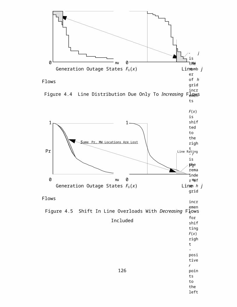
. Summary Of The Process For Removing Line Overloads· line j with the greatest probability of overload is found,

· an increment Dy is assigned for removal in line j,

· the increasing flow generators are convolved,

· the two dimensional F(x,y) is set up,

· the decreasing flow generators are convolved into F(x,y),

· a partial density 2-D function is created from F(x,y),

· the most offending generator-load pair is taken from the LST,

· the partial distributions are shifted to remove the line overloads,

· the line overload distributions are stored in a temporary array T(x),

· the T(x) is added to FG(x),

· the other lines jointly affected by the generator-load pair are adjusted also, and

· the process is repeated until all line overloads are removed.

Load Shedding MethodologyA number of lines can be overloaded as a result of the convolution process

described in Chapter 8. The probabilities of line overloads vary widely, as does the

range of MW loadings. Figure 10.2 shows an illustration of several line loadings.

Dy

p

line j overloads shifted left by Dy

Fj(y) Fj(y)= Pr [random line MW > y]

y

Rj increasing MW

Figure 10.2 Incremental Unloading Of Line j

136

Line j with the highest probability of overload Fj(y=Rj) is selected to be

unloaded first. It has the largest amount of time in which the line will be overloaded

for the specific p and Dy segment (shaded block) shown. The removal of this shaded

block shifts the line overloads to the left (dotted line) by Dy MW for the region y>Rj .

The value of p is given in Equation 10.1.

p = 1D

D

yF y dyj

R

R y

j

j

( )+

ò » F R F R yj j j j( ) ( )+ + D2

for small Dy

(10.1)

The removed Dy increment on line j must be transferred to a specific

generator and load. A generator and load most responsible for causing the overload

on line j does exist, so this generator-load pair needs to be identified and

correspondingly reduced in output, consistent with the reduction in line j loading.

.1 .2v -.2 -.1

-.15v

.05 .3 Line j -.35v

-.2 -.1

.2v

.25 -.18v

Figure 10.3 Example Of Real And Virtual Distribution Factors For Line j

Figure 10.3 shows an example of several real and virtual (v) generators that

are causing incremental loadings on line j. The virtual generators are used primarily

to develop line distribution factors associated with loads. The line j distribution

factor for each source is shown above the bus. The thin lines represent an

137

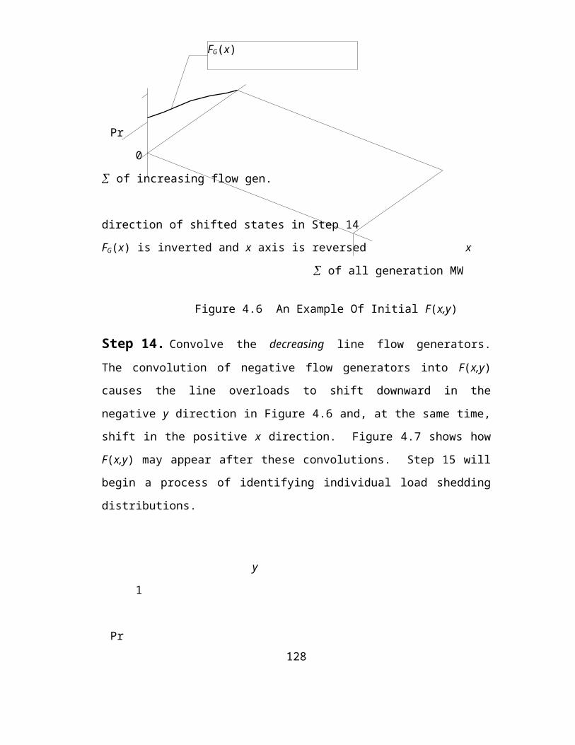
interconnected transmission network. Notice that the real generators to the left

(.1, .05, .3, .25) are causing an increase in flow on line j (direction of the arrow), and

the virtual generators on the right (-.35v, -.15v, -.18v) are also causing an increase in

flow on line j. The largest flow is caused by the pair, .3 and -.35v. Together, these

have a distribution factor on line j of .3-(-.35)=.65. Therefore, the generator with

the .3 factor and the load with the -.35 factor will be reduced by Dy/.65 MW with

probability p. This change in generator output will need to be reflected in the FG(x)

function and in the other line distributions. The change in FG(x) is discussed next.

Figure 10.4 shows the relationship between the generation outage distribution,

FG(x), and the generation availability distribution, FA(x). Each function is the

complement of the other, and their x axes are reversed. FA(x) has an interesting

property we will now use.

FG(x) = Pr outaged MW > x

FA(x) = Pr available MW > x

0 x MW 0 x MW

Figure 10.4 Equivalency Of Outage And Availability Distributions

Convolve the real generators with positive (line j) distributions into an Fj(y)

temporary line distribution function and into an FA(x) temporary generation

availability function. Figure 10.5 shows that the resulting curves have a similar

appearance, although they are different because the incremental x and incremental y

values that are being convolved into each function are different sets of numbers.

138

xmax

FA(x) Fj(y)

0 x MW SCk 0 y MW ymax

Figure 10.5 Convolving Only The Positive Distributions On Line j

In Figure 10.5, xmax is the MW sum of all generators having positive

distributions in line j, ymax is the maximum positive MW flow on line j equal to the

sum of all positive MW incremental line flows, and the dashed lines represent the

maximum line j MW rating for the positive and negative line flow directions.

Figure 10.6 shows how the distributions appear if the most offending

generator-load combination with the .65 line j distribution factor is deconvolved or

removed. In this example, line overloads are completely removed by corrective

action on one generator-load pair. However, the complete removal of this generator

is an overcorrection. The offending generator-load pair will be able to operate for a

portion of the time at varying load levels and still not overload line j.

xmax

FA(x) Fj(y)

0 x MW SCk 0 y MW ymax

Figure 10.6 Distributions With The Most Offending Generator-Load Removed

Figure 10.7 shows the portion of the line distribution that is not allowed when

the offending generator-load pair is put back in the system. The shaded portion of

139

the line j distribution is not allowed to exist, and is to be mathematically removed. In

removing the line j overload, consideration is given to how this affects the FA(x)

distribution. One apparent relationship in Figure 10.7 is that a Dy MW change on

line j corresponds to a Dx=Dy/.65 MW change in the generator-line pair MW.

distributions not allowed

xmax

FA(x) Fj(y)

Dx Dy

0 x MW SCk 0 y MW ymax

Figure 10.7 Portion Of Probability Space Not Allowed To Offending Generator-Load

In addition to the Dx=Dy/.65 being true in Figure 10.7, the areas of the two

shaded regions are also related by the same .65 (from Figure 10.3) distribution factor.

This is due to an (almost true) assumption that every deterministic configuration in

the binary tree (in Figure 10.1) that reduces the flow on line j uses the same .65

factor. The areas are directly calculated from these individual states that are in

proportion. Therefore, the areas are also in the same proportion.

140

xmax

FA(x) Fj(y)

Dx Dy

0 x MW SCk 0 y MW ymax

Figure 10.8 The Effects Of Adding A Negative Flow Generator

If there were no generators causing negative flows in line j, the overload

portion of FA(x) could be mapped directly back to FG(x) since there is a one-to-one

relationship between the two functions. However, the presence of generators causing

reductions in the overloads on line j must be taken into account. Figure 10.8 is an

example of how the line overloads in Figure 10.7 are dispersed in both the line j

distribution and the FA(x) distribution. In the example shown, the decreasing or

negative flow generator is given an FOR » 20% for easy visualization. In each

distribution, the new generator causes the original line overloads (shaded areas in

Figure 10.7) to be split into 80% and 20% states for the new generator’s success and

failure states, respectively. The 80% success states are shifted to the right in FA(x) by

the MW rating of the generator and are shifted to the left in the Fj(y) by the

distribution factor times the MW rating of the generator.

Notice that 80% of the original line overloads are no longer overloading line j

after the negative flow generator is added. If FG(x) had been adjusted based only on

the positive distribution factor generators, the amount of load shedding would have

been greatly overstated. The lesson taught by this example is that all generator

outage states must be convolved together before applying load shedding.

141

Figure 10.8 contains sufficient information to link the removal of the line

overloads to the FA(x) and FG(x) distributions. The original xmax and ymax locations are

stationary as the negative flow generators are included. Also, the relationship

Dx=Dy/.65 is still true, as well as the .65 factor relationship between the two smaller

shaded areas in Figure 10.8. The two larger shaded areas are no longer of interest

since they do not represent any problems in the system.

The steps given in this example show a need for a more general way to map

the locations of line j overloads and FA(x). A grid can be constructed to meet this

general need as shown in Figure 10.9. A specific state with a probability p in the

binary tree in Figure 10.1 will have a specific location on this two dimensional grid.

All the states in the binary tree have unique locations on this grid, which maps all

possible combinations of line flow and generation availability.

F(x,y)

Fj(y) p

y x FA(x)

Figure 10.9 F(x,y) Maps All Combinations Of Line And Generation States

142

The overload increment Dy (in Figure 10.2) has been removed from the line j

distribution by shifting the overloads on line j to the left by Dy. The objective now is

to map a corresponding shift to the temporary FA(x) function. The examples given

thus far are a guide on how to proceed in doing this mapping.

y

1

Pr

0

xmax

xmax = S of increasing flow gen.

distribution function movement

FA(x) x

of all generation MW

Figure 10.10 Initializing F(x,y) With Line Overloads Due To Increasing Flows

Generators with incremental increasing1 flows on line j are convolved into a

temporary line distribution function Fj(y) using the generator states in Table 3.3, the

line distribution factors calculated in Chapter 7, and the procedures in Chapter 8.

The incremental decreasing flows require the use of F(x,y) to find the specific

locations between Fj(y) line overloads and FA(x). F(x,y) is initially set to zero

1 Note that these flows were referred to as positive flows in the previous examples in this chapter. A better description is increasing flows rather than positive flows since negative flows can also cause a line to overload. Increasing flows are those causing a line to become more overloaded in a chosen direction, and decreasing flows are those that reduce the overload in this same direction. Since lines are tested for overload in both directions, the roles of increasing and decreasing incremental line flows are reversed, depending on which direction a line is being tested.

143

PQ x = 30%

everywhere, except the left-most axis is set to F(x=xmax ,y)=Fj(y). Figure 10.10

shows how F(x,y) is initialized.

Figure 10.10 shows that the process of convolving decreasing line flow

generators will shift the line distributions across the x-y plane. This shifting requires

an interpolation using four adjacent points in F(x,y) surrounding a point to be

interpolated. Let 0<rx<1 and 0<ry<1 between grid increments and the four local

discrete points on the surface of F(x,y) be defined as shown in Figure 10.11.

T1 T2

y ry

T3 T4

rx

x

Figure 10.11 Linear Interpolation of F(x,y)

The convolution of a decreasing line flow generator into F(x,y) is given in

Equation 10.2. This is a two state PL equation for convolving generator k into line j

on the F(x,y) distribution. A three state generator will have an extra (Hj,k×Dk ) term.

F(x,y)after= F(x,y)before×EFORk +F(x-Ck , y+(Hj,k×Ck ) )before×(1-EFORk) (10.2)

In the above equation, the generator outage state is not shifted. The generator

available state is shifted downward according to -(Hj,k×Ck)/hy = jy + ry and to the right

according to Ck /hx = ix + rx. The hx is the x axis grid MW spacing and hy is the y axis

grid MW spacing. The ix + rx is the integer and fractional x shift distance pointing to

the left. The jy + ry is the integer and fractional y shift distance pointing upward. This

is consistent with Figure 10.11. Equation 10.2 is used to update the discrete array

points F(ih x+b x , jh y+b y). The i and j are positive increasing steps upward and to the

right. The bx and by are the xmax shown in Figure 10.5 and the Rj in Figure 10.2

144

respectively. If F(x,y) is a FORTRAN array of discrete points, then the two state

convolution equation is written as

F(i , j) = EFORk×F(i , j) +

(1-EFORk)×[T1rxry + T2(1-rx)ry + T3rx(1-ry) + T4(1-rx)(1-ry) ] (10.3)

where the T values are determined by the location of the point to be interpolated

according to ix + rx and jy + ry and the relative locations of the T points shown in

Figure 10.11. A three state generator simply has an extra interpolated shift point.

Figure 10.12 shows what F(x,y) might look like after the convolution of

decreasing flow generators.

y

1

Pr

0

increasing flow gens.

FA(x) x

of all generation MW

Figure 10.12 An Example Of F(x,y) With All Generators Convolved

The F(x,y) is a cumulative distribution in both x and y. However, what is

needed are the point probability densities within the F(x,y) space. These can be

thought of as corresponding to the specific state probabilities shown in the binary tree

145

PQ x = 20%

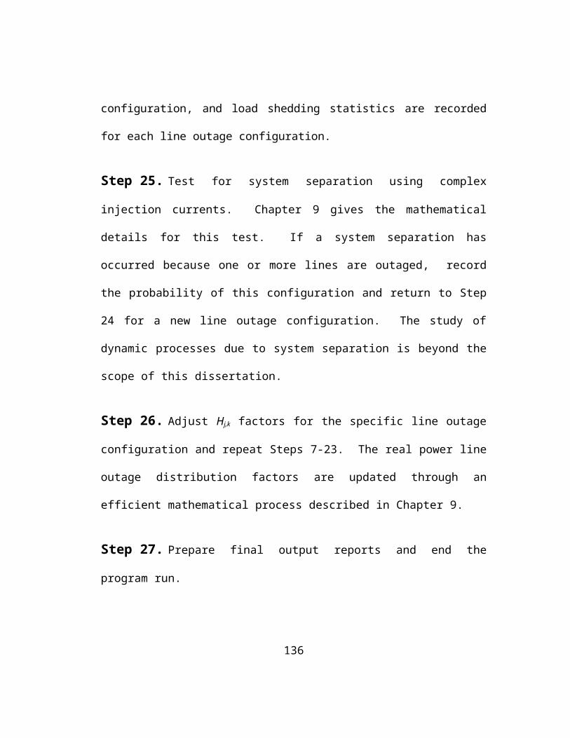
in Figure 10.1. By knowing the probability of these states and their locations, the

shifting of line j overloads (down to the line rating) produces a trace on the FA(x)

axis. Figure 10.13 shows how shifting a single state p on the F(x,y) plane maps to the

line loading and the generation availability distributions. The shaded areas show the

Dx and Dy shifts as a function of the location of p on the x-y surface.

y

1 Fj(y)

Pr

0

xmax

xmax = S increasing flow Ck

initial p

FA(x) x

SCk

Figure 10.13 Discrete State With Probability p Shifted To Reduce Line Overload

Figure 10.14 shows that a cumulative distribution of three p states (shaded)

can be shifted and mapped to both the Fj(y) and FA(x) functions. The shifted states

map in opposite directions on the line and generation distributions.

146

y

1 Fj(y)

p

Pr

0

xmax

xmax = S increasing flow Ck

FA(x) x

SCk

Figure 10.14 Distribution of States Shifted To Reduce Line Overload

Figure 10.14 shows that a distribution of states can be shifted and mapped to

the FA(x) distribution in a precise manner. The movement of the three p states on the

paths indicated by the three arrows from their initial locations in the interior of the x-

y plane to the y=Rj axis effectively eliminates the line overload and maps correctly to

the generation distribution.

F(x,y) is converted to a set of partial density functions Fp(x,y) by subtracting

adjacent x rows for all y. Equation 10.4 performs this operation. The resulting

Fp(x,y) are a series of distributions at every x grid increment oriented as shown in the

shaded distribution in Figures 10.14 and 10.15.

Fp(x,y) = F(x,y)-F(x+hx ,y) (10.4)

The hx in Equation 10.4 is the discrete x axis grid spacing in Figure 10.14. Figure

10.15 below illustrates one of these distributions being shifted back to the x axis.

147

y

1

Pr

0

increasing flow gens.

x

of all generation MW

Figure 10.14 Shifting Partial Line Overload Distributions To The Generation Axis

The process of shifting the overloads in Fp(x,y) can now begin. Select the m-

n generator-load (virtual generator) pair with the greatest increasing flow line j

distribution factor Hj,m-n. This pair should be at the top of the load shedding table

(LST). An LST is constructed once and used repeatedly as line j is being unloaded.

The LST should contain a list of generators, loads, and increasing flow distribution

factors in descending order. The LST can also log other statistics, such as how much

power and energy has been decreased in each generator.

The next step is to shift the Fp(x,y) partial distributions as a function of the

LST distribution factor. The shifting process moves the partial distributions as

shown in Figure 10.14. The Dy/Dx movement slope is equal to the distribution factor

Hj,m-n defined in Equation 7.1. The partial distributions are shifted and added to an

array T(x), which is a temporary holding tank for the distributions as they arrive at

the lower x axis. The partial distributions are added to T(x) as they are shown in

Figure 10.14. The T(x) array captures all the incremental Fp(x,y) (shifted p states)

information. The T(x) x axis is inverted and scaled (if necessary) to align with the

148

PL x = 30%

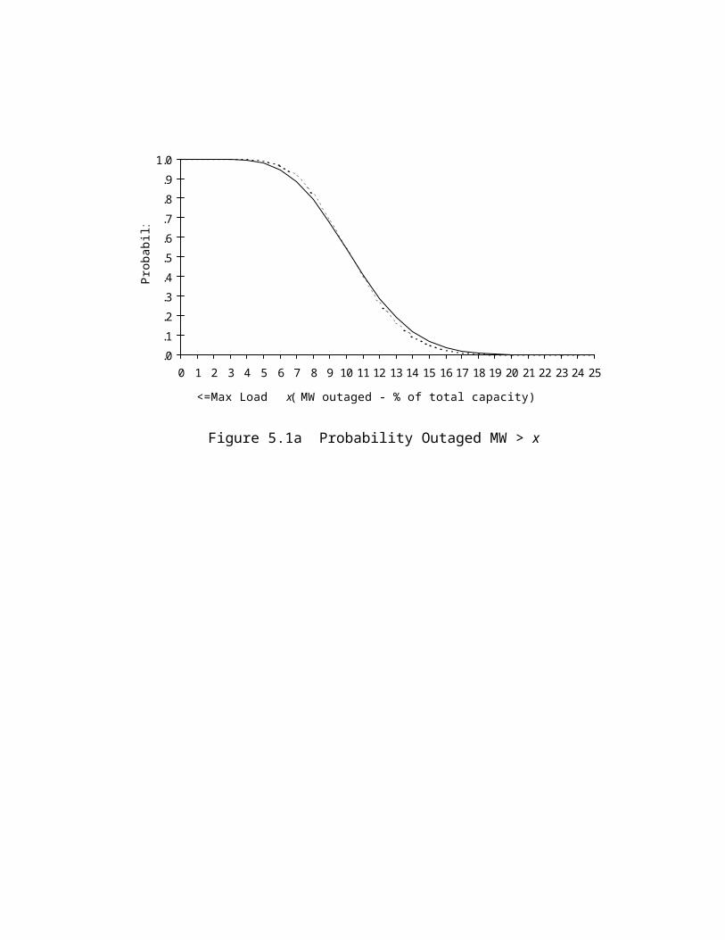
FG(x) x axis. Figure 10.15 shows the T(x) array being added to FG(x). After this

summation, the T(x) is reset to zero for the next line increment to be unloaded.

1

Pr

0

Figure 10.15 Generation Unreliability Due To Transmission Constraints

Thus far, only the one small Dy increment in Figure 10.2 has been unloaded

and mapped to FG(x). The shifted states on line j are due to the m-n generation-load

pair reducing their MW by an amount Dy/Hj,m-n at a probability p. Line j overload

states are reduced by Dy MW. This m-n generator-load pair may be contributing to

the overloads of other lines l. Each of these other overloaded lines l will have a

distribution factor Hl,m-n increasing the overload in line l. For lines with Hl,m-n >0, use

Equation 10.5 to estimate the reduction in loadings by an amount Dyl for lines l.

Dyl = (Dy)(Hl,m-n)(Hj,m-n)-1 . (10.5)

Equation 10.5 has an assumption that the overloads on the other lines l occur

jointly with line j because the same set of generators are assumed to be overloading

both line j and the other lines l. Simple examples show this can only be true if the

line overload increments are selected in decreasing order of overload probability and

if the same set of generators are causing the overloads. Figure 10.16 is an example of

149

1 hr

tightly coupled lines A, B (2 lines), and C in combinations of series and parallel. The

same offending generators cause proportional line overloads on all four lines jointly.

A

B C

Figure 10.16 Tightly Coupled Lines In Series And Parallel

The assumption that the same set of generators are causing the line overloads

is most incorrect for overloaded lines that are weakly coupled electrically; which

usually means they are widely separated physically. For this situation the assumption

that the overloads occur jointly is probably wrong. However, the use of Equation

10.5 for this situation does not introduce an unacceptable amount of error because the

electrical coupling is low and Equation 10.5 produces very small Dyl adjustments

compared with the Dy adjustment in line j. The error introduced will cause the load

shedding EUE to always be understated. The examples in Chapter 12 show that this

heuristic can give excellent results if the system is not too overloaded and that it does

a poor job of estimating the load shedding if the system is extremely overloaded.

The large electric power systems are very reliable, so this load shedding model

should produce reasonable results for realistic systems. Once all the lines have had

their line overload distributions shifted due to the offending generator-load pair, the

entire process is repeated.

150

Chapter 11

Large System Examples

This chapter gives two large system examples. The first example tests the

linearity of the fast line and generator outage model presented in Chapter 9 against

full AC load flow solutions for combinations of up to one generator and three lines

outaged simultaneously. The first example also appears in [55]. The second example

is a large system planning study in which the reliability benefits of an additional 480

MVA autotransformer are studied. The City of Austin studied this addition to offset

the decrease in reliability due to a scheduled power plant retirement. The second

example also appears in [1].

Example OneFigure 11.1 shows the test system used to compare the new multiple line and

generator outage model presented in Chapter 9 with full AC load flow solved cases.

D A1

City of Austin A2 ERCOT

138 kV System L1 345 kV System

P L2

Figure 11.1 City of Austin Large System Network Test Case

In this example, the City of Austin load level is maximized to 2334 MW as a MaxGen

configuration load flow case with 74 MW COA transmission losses. The four

autotransformers A1...L2 are loaded to a total of 1143 MW and 430 MVAR in the

MaxGen configuration base case. Internal COA generation at D is 910 MW. No

151

COA lines are overloaded in the base case, and all voltages are nominal. The base

case has all generators operating at maximum output levels with area loads scaled to

equal area generation owned plus firm purchases less firm sales less area loss.

All the line outage cases shown in Tables 11.1 and 11.2 are deterministic

solutions using the ‘zipflow’ model presented by Preston, Baughman, and Grady in

[55] and are compared with full AC load flow solutions. No probabilistic line flows

are modeled in this test. The purpose of this exercise is to test the ability of the

zipflow to accurately predict MW line flows for multiple lines and generators

outaged. The zipflow solutions are the sums of large numbers of linear real factors.

The difference between Table 11.1 contingencies and Table 11.2 contingencies

is that Table 11.1 has no outaged generation, and Table 11.2 has an additional loss of

710 MW generation at bus D. The line outages between the two tables are identical.

Each numbered case represents a different set of lines ‘out’ of service. The results are

shown inside the boxes which consist of

· the MW flow from the linear summation of flows process,

· the MW flow from the AC load flow,

· the difference shown as an error in MW, and

· the percentage error with reference to the line rating.

The columns are descriptors of the case study and the six circuits monitored. The rows

are the different contingencies simulated. Percentage errors are the MW differences

between the two solution methods referenced to a 480 MVA line rating for all the lines

and transformers listed. Errors less than one percent are shown as <1% and are

considered by the author as being very accurate. The ‘base’ case errors in Table 11.1

should be zero, but are not zero, due to differences in the MaxGen configuration load

flow in the PLF model and the independently solved AC solutions.

152

Table 11.1 Transmission Line Flows Due To Line Outages,

No Generation OutagedZipflow - AC Load Flow = Zipflow Error

CaseLineA1

LineA2

LineD

LineL1

LineL2

LineP

base-277.0-277.2

0.2<1%

-270.6-270.8

0.2<1%

260.9259.9

1.0<1%

-297.1-297.3

0.2<1%

-297.1-297.3

0.2<1%

334.7332.6

2.1<1%

1 out-423.8-416.5

-7.31.5%

225.6223.9

1.7<1%

-329.1-332.2

3.1<1%

-329.1-332.2

3.1<1%

380.2381.9

-1.7<1%

2-313.3-315.8

2.5<1%

-306.1-308.5

2.4<1%

310.0312.7

-2.7<1%

out -505.3-499.1

-6.21.3%

271.6264.9

6.71.4%

3 out out 103.3107.5

-4.2<1%

-438.5-442.4

3.9<1%

-438.5-442.4

3.9<1%

538.4536.8

1.6<1%

4 out -486.3-482.9

-3.4<1%

275.4278.2

-2.8<1%

out -567.7-566.5

-1.2<1%

316.1312.8

3.3<1%

5-519.1-517.2

-1.9<1%

-507.1-505.2

-1.9<1%

591.3589.1

2.2<1%

out out -91.7-92.7

1.0<1%

6 out out 148.1158.3-10.22.1%

out -795.2-794.9

-0.3<1%

480.9473.8

7.11.5%

7 out -876.6-864.5-12.12.5%

591.3593.7

-2.4<1%

out out -91.7-92.9

1.2<1%

153

Table 11.2 Transmission Line Flows Due To Line Outages,

710 MW Generation OutagedZipflow - AC Load Flow = Zipflow Error

CaseLineA1

LineA2

LineD

LineL1

LineL2

LineP

base-289.2-294.4

5.21.1%

-282.5-287.6

5.11.1%

365.7377.6-11.92.5%

-280.0-279.9

-0.1<1%

-280.0-279.9

-0.1<1%

341.8339.9

1.9<1%

1 out-442.4-442.5

0.1<1%

328.8338.7

-9.92.1%

-313.4-317.2

3.8<1%

-313.4-317.2

3.8<1%

398.4392.4

6.01.3%

2-323.5-330.5

7.01.5%

-316.0-322.9

6.91.4%

411.9426.1-14.23.0%

out -476.1-470.6

-5.51.1%

282.4276.6

5.81.2%

3 out out 201.1214.1-13.02.7%

-427.5-435.1

7.61.6%

-427.5-435.1

7.61.6%

554.5557.6

-3.1<1%

4 out -501.9-505.3

3.4<1%

376.2389.2-13.02.7%

out -540.6-541.8

1.2<1%

328.4327.0

1.4<1%

5-517.4-520.5

3.1<1%

-505.3-508.5

3.2<1%

677.0681.6

-4.6<1%

out out -59.9-60.3

0.4<1%

6 out out 244.8262.3-17.53.6%

out -775.4-783.2

7.81.6%

498.4496.4

2.0<1%

7 out -873.6-870.6

-3.0<1%

677.0684.3

-7.31.5%

out out -59.9-60.4

0.5<1%

154

The results show that the summation of linear real incremental flows can be

used to construct MW line flows that are in good agreement with full AC load flow

solutions. The process of adjusting the H line distribution factors in Chapter 9 to

accommodate the triple contingency line outages works well, as evidenced by the

relatively low errors in Table 11.2. The results show very large variations in power

flows on each line due to the multiple line and generator outages. The combination

of multiple lines and generators outaged simultaneously, and modeled as sets of

linear factors, is new to the industry. The results presented here and in [1, 34, and

55] are outstanding, considering that this type of model has not been previously

constructed.

Example TwoAn example is presented showing how the PLF model presented in this

dissertation has been applied to a real planning problem at the City of Austin Electric

Utility Department. The COA system in this example is a ~1700 MW peak demand

69 kV and 138 kV system connected through a number of 480 MVA

autotransformers to the ERCOT (Electric Reliability Council of Texas) 345 kV

system. The ERCOT system load flow and generator reliability planning data bases

have ~ 300 generators, 4200 buses, and 5200 lines. This is a large system because

the generator and line outage configurations are far too numerous to enumerate.

The reliability of the COA system is highly dependent on its autotransformers

to supply emergency reserve power from ERCOT as well as 950 MW COA owned

generation on the 345 kV grid. The autotransformers become more critical when a

550 MW plant (Holly) centrally located in the COA system is retired in a few years.

Presently, the COA has two bulk transmission substations, Austrop and Lytton. Each

station has two 345/138 kV autotransformers. A third 345 kV substation called

Garfield has been constructed and will soon be energized with one 480 MVA

autotransformer. Figure 11.2 shows the layout.155

The COA power supply reliability is a function of the ERCOT power supply

reliability and the reliability of the transmission network delivering the ERCOT

power. Autotransformer outages are severe because they are few in number in the

COA system and because their repair times are long (six months to one year). The

COA autotransformer catastrophic failure experience is consistent with [66].

Austrop

City of Austin ERCOT

Garfield

138 kV System 345 kV System

Lytton

Figure 11.2 City of Austin 345/138 kV 480 MVA Autotransformers

For study purposes, a pessimistic autotransformer forced outage rate of 4% is

used. The study is repeated using a more optimistic 2% autotransformer FOR to see

if the study results are sensitive to the FOR values chosen1.

Figures 11.3 and 11.4 show the additional EUE caused by autotransformer

failures for all COA autotransformer outages through N-3 triple simultaneous

outages. Up to 60 lines in the COA system are monitored for probabilistic overload.

Approximately 2300»1090 generation outage configurations are modeled for all

ERCOT generators.

1 The autotransformer FOR assumption did not change the relative results of this study.

156

1E-06

1E-05

1E-04

1E-03

1E-02

1E-01

1E+00

1E+01

1E+02

1E+03

65 67 69 71 73 75 77 79 81 83 85 87 89 91 93 95 97 99Percent of Generation Capacity

EUE

- MW

H

4

5

3

2

1

Figure 11.3 COA EUE With Autotransformer FOR=.04

1E-06

1E-05

1E-04

1E-03

1E-02

1E-01

1E+00

1E+01

1E+02

1E+03

65 67 69 71 73 75 77 79 81 83 85 87 89 91 93 95 97 99Percent of Generation Capacity

EUE

- MW

H 4

5

3

2

1

Figure 11.4 COA EUE With Autotransformer FOR=.02

157

1 hr

discussed in the text

p(r)=r+.5

Pr

The following conditions are modeled in both Figures 11.3 and 11.4.

· Curve 1 is the total generation supply EUE available to the COA with no

transmission constraints. This is the integral of the FG(x) for ERCOT and

made proportionately available to the COA system.

· Curve 2 represents the additional transmission EUE with 540 MW of Holly

generators not retired and with no Garfield autotransformers.

· Curve 3 shows the increase in EUE with the Holly generators retired.

· Curve 4 is the decrease in transmission EUE as one autotransformer is added to

the Garfield substation when Holly generation is retired. This transformer

already exists in the system.

· Curve 5 is the decrease in transmission EUE as two autotransformers are added to

the Garfield substation when Holly generation is retired. Note that the second

autotransformer at Garfield is the one under study and is shown lighter than the

other transformers in Figure 11.2.

The study shows that two autotransformers at Garfield bring the reliability

back to about the same level as before the Holly generators are retired. This holds

true for both the 4% and 2% autotransformer FOR as shown in Figures 11.3 and

11.4. The extra autotransformer is justified with the Holly generation retired.

Conventional load flow studies using deterministic enumeration contingency

methods did not show a value for the additional autotransformer at the Garfield

substation. Only the full set of generation outages for all generators in ERCOT

combined with the triple contingency outages of autotransformers serving the COA

brought out the probabilistic value of the new transformer. The completion of the

PLF computer program made it possible for the first time to run this study.

158

Chapter 12

Test Cases Using IEEE RTS

The purpose of this chapter is to benchmark the PLF method presented in this

dissertation against an enumerated solution using a linear program with optimal load

shedding. Because the number of configurations increases exponentially with system

size, a very small system must be used in this test if all generator outage possibilities

are to be enumerated. The IEEE Reliability Test System [28,30] is selected as a

system with enough transmission and generation detail to make the test nontrivial.

Before describing the test setup and results, a description of the LP solution is

needed.

Linear Programming ModelA separate linear programming model was written several years ago within

the PLF program to fully enumerate all generation outage configurations in very

small networks. The program code was added for the purpose of testing different

convolution concepts as they were being developed. The LP solution itself is not a

part of the probabilistic load flow solution methodology. It has been added only to

verify convolution and load shedding results.

The Hi,k factors for every line i and generator k are directly usable in the LP

constraints and objective. The LP objective is set up to maximize the generation

power delivered. If no transmission constraints exist, the generators not outaged

operate at maximum output. This is a no load-shedding case. Transmission

constraints (line MW flow exceeding the line rating) reduces the delivery of power to

individual load areas. The LP finds the solution delivering the greatest amount of

power to loads. Equations 12.1 and 12.2 show how a single line i is tested for

overload in both directions.159

One line flow direction is

Hi,1×U1+Hi,2×U2+Hi,3×U3+...-Hi,Ng+1×V1-Hi,Ng+2×V2...£ Ri ,(12.1)

and the other direction is

-Hi,1×U1-Hi,2×U2-Hi,3×U3-...+Hi,Ng+1×V1+Hi,Ng+2×V2...£ Ri (12.2)

where Uk is the generator k output power in MW, Vi is the total virtual generation

MW (load to be shed) in area i, Hj,k is the real power distribution factor for line j and

generator k or virtual generator Ng+i, and Rj is the line j rating. Each generator has a

maximum power set by the constraint Uk £ Ck where Ck is the MW rating of each

generator k. The objective function is to maximize the sum of all U values.

Each generation configuration is enumerated by stepping through all the

possible combinations of generator outages, one configuration at a time. In each

configuration, the line flows are calculated using the distribution H factors. If no

lines are overloaded, the LP is not used since there is no load shedding for that

generation configuration. If one or more lines are overloaded, the LP is set up and

solved. The probability of each generation configuration is calculated along with the

MW load shed for each configuration. The statistics are assembled and displayed in a

manner similar to the binary tree shown in Figure 3.15.

IEEE Reliability Test System The IEEE Reliability Test System has been modified by defining three load

areas. Dividing the RTS into three areas allows testing to be done on a nontrivial, but

small multi-area model. Figure 12.1 shows the RTS system with the three load areas,

North (buses 14-22), Central (buses 3,4,6,9-13,23,24), and South (buses 1,2,5,7,8).

160

17 18 21 22

16 19 20

Area 1 15 14 North 23

Area 2Central 13

24 11 12

3 9 10

4 6

Area 3 5 8 South

1 2 7

Figure 12.1 IEEE Reliability Test System

161

In order to keep the full enumeration run time reasonable, generators are also

combined at each load flow bus. Table 12.1 shows the new generator data. Each

generator has a maximum capacity equal to the sum of all the original generation

capacity at each bus with generators in the original RTS data. The new generators

are two state models with the EFOR set to the forced outage rate of the largest

generator originally on the bus.

Table 12.1 Modified RTS Generator Data # Name Area MW EFOR Bus# 1 HYDRO A1 300 0.010 22 2 COAL 1 A3 192 0.020 1 3 COAL 2 A3 192 0.020 2 4 FS#6 1 A3 300 0.040 7 5 COAL 3 A1 215 0.040 15 6 COAL 4 A1 155 0.040 16 7 COAL 5 A2 310 0.040 23 8 FS#6 2 A2 591 0.050 13 9 FS#6 3 A2 350 0.080 2310 NUCL 1 A1 400 0.120 1811 NUCL 2 A1 400 0.120 21

The RTS MaxGen configuration load flow has no overloaded lines when all

lines are in service. The probabilistic line overloads are small and contain little load

shedding energy. The RTS is well known as a very reliable transmission system, and

modifications are usually made to increase line overload problems in the RTS. The

purpose here is to test the PLF heuristic against an independent LP solution in which

the LP optimizes load shedding for every configuration of generation outages. If no

overloaded lines are found, there is no need for the LP, and there is no transmission

load shedding. To create a progressively weaker transmission system, all lines in the

RTS are derated in 20%, 40%, and 60% steps to create probabilistic overloads. This

creates many overloaded lines. Results are shown in Figures 12.2 and 12.3 for line

deratings to 80%, 60% and 40% of normal capacity.

162

1E-06

1E-05

1E-04

1E-03

1E-02

1E-01

1E+00

1E+01

1E+02

30 35 40 45 50 55 60 65 70 75 80 85 90 95 100

EU

E -

MW

H

Figure 12.2 RTS Transmission EUE by Area Vs Percent Load For 80% Line RatingsComparing Convolution Results With Linear Program Solution Results

1E-06

1E-05

1E-04

1E-03

1E-02

1E-01

1E+00

1E+01

1E+02

1E+03

30 35 40 45 50 55 60 65 70 75 80 85 90 95 100

EU

E -

MW

H

Figure 12.3 Total Transmission EUE Vs Percent Loading For All LinesComparing Convolution Results With Linear Program Solution Results

163

F(x,y)line overload states in Fig. 10.7Rj(y) £ y £ max. line flow

line overload states

line overload states shown in Fig. 10.8

MW Range Not Overloaded

F(x,y) surface as a set of discrete points

FG(x)+ T(x)

FG(x)

Fp(x,y)

The 80% line ratings case has several lines probabilistically overloaded:

line 6-10 of 122%, line 7-8 of 201%, line 8-9 of 126%, line 8-10 of 112%,

line 14-16 of 118%, line 16-17 of 116%, and line 16-19 of 106%. The PLF

heuristic gives excellent results for this case with lines derated to 80% of normal.

The 40% line ratings case shows that the PLF heuristic performs very poorly

and calculates a much too small transmission EUE compared with the LP solution

when all lines are heavily overloaded (in both directions). The error was introduced

in the step 20 process of unloading lines using only the increasing line flows

(increasing in both directions). Step 20 assumes the generator-load combinations

causing incremental line flows in opposite directions are too weakly coupled to be of

significance. This assumption is true only when the transmission system is reliable

with low probabilities of lines being overloaded. If lines in close proximity are

heavily loaded in both directions, then the assumptions made in the heuristic are no

longer true. The 60% line ratings case shows intermediate error results as expected.

The ERCOT system appears to perform more like the RTS case with 80% line

deratings than the 40% case, so the PLF model is operating in an environment in

which the load shedding heuristic is most accurate. Another point to be made is that

the PLF error decreases as the system is made more reliable. The enumeration

methods increase in error as the system is made more reliable because they cannot

uncover enough failure configurations to calculate the LOLP and EUE to a precision

of two digits.

164

Chapter 13

PLF Program Output ReportsLoad Flow Reports

This chapter will step through the computer program’s output reports for the

286 generator network. This is a highly shortened report showing only a few lines of

data for each type of output. The actual report for this one case is >300 pages. The

reports below are listed in the same order as they are calculated and displayed. The

first output report is the load flow solution shown in Table 13.1. Points of interest

are given an to draw attention to the information.

Table 13.1 MaxGen Configuration Load Flow Initial Report

Case Title: 1996 ERCOT RELIABILITY TEST SYSTEM

Base MVA = 100.0

Load Flow Solution Monitor: Number of buses = 2231 5500 max Number of generators = 147 Number of circuits = 3092 6500 max Number of xformers = 553 1200 max Number of areas = 9 20 max Swing Bus = 4546 Read load flow data = 0h 0m 3s regulated bus 6235 reassigned to bus 6230 regulated bus 6444 reassigned to bus 6443

load flow generators not having probability data: 799 TEXASAM 138 area 11 30.0 MW 15.0 MVAR 4181 DIAMON 8 138 area 4 4.0 MW 0.1 MVAR 4182 DS BAT 8 138 area 4 25.0 MW 0.0 MVAR 4194 DOW A 8 138 area 4 262.0 MW 0.0 MVAR 4234 EXXON 8 138 area 4 18.0 MW 0.0 MVAR 4492 PSARCO 8 138 area 4 491.0 MW 103.7 MVAR 4684 TEXGLF 8 138 area 4 82.0 MW 12.7 MVAR 6762 SAPS 1G14.4 area 6 24.0 MW -6.7 MVAR 8032 AMS #1 13.8 area 8 19.0 MW 0.0 MVAR these generators are assumed to have 95% availability No of prob generators = 286 350 max

165

Table 13.1 Load Flow Initial Report (cont.)

GENERATION SUMMARY (MW):

A# AREA PHYSICAL EXPORTED IMPORTED NET INTERCHG -- ------ -------- -------- -------- -------- -------- 1 TU 25208. 1820. 558. 23946. 1262. 4 HLP 16587. 2218. 1740. 16109. 478. 5 CPSB 3699. 0. 700. 4399. -700. 6 WTU 1929. 119. 33. 1843. 86. 7 LCRA 2854. 588. 3. 2269. 585. 8 S.TEX. 4380. 219. 767. 4928. -548. 9 COA 910. 203. 1124. 1831. -921. 10 COA9 540. 406. 439. 573. -33. 11 TMPP 2090. 91. 300. 2299. -209.

Matrix factoring time = 0h 0m 2s Matrix initial size = 10915 20000 max Matrix final size = 10047

************************************* * Generation is at maximum capacity * * Bus loads have been scaled upward * * Area interchanges have been reset * * Generator Qmn/mx is now unlimited * *************************************

load flow solution monitor ... iter 0 bus 4737 perr= 501.68 bus 7334 qerr= 50.42 0.11 sec iter 1 bus 4488 perr= 28.18 bus 4488 qerr= 166.08 0.22 sec iter 2 bus 9187 perr= 12.98 bus 1032 qerr= 25.25 0.22 sec iter 3 bus 4726 perr= 1.11 bus 4726 qerr= 8.10 0.27 sec iter 4 bus 6480 perr= 0.67 bus 4726 qerr= 3.58 0.22 sec iter 5 bus 4726 perr= 0.23 bus 4726 qerr= 1.59 0.27 sec iter 6 bus 6480 perr= 0.12 bus 4726 qerr= 0.71 0.22 sec iter 7 bus 4726 perr= 0.04 bus 4726 qerr= 0.31 0.27 sec iter 8 bus 6480 perr= 0.02 bus 4726 qerr= 0.14 0.22 sec iter 9 bus 6763 perr= 0.01 bus 4726 qerr= 0.06 0.22 sec iter 10 bus 4548 perr= 0.01 bus 4726 qerr= 0.03 0.27 sec iter 11 bus 4548 perr= 0.01 bus 8263 qerr= 0.02 0.22 sec iter 12 bus 4548 perr= 0.00 bus 8263 qerr= 0.01 0.27 sec

166

a load flow solution has been found iteration time = 3 sec total load flow time = 9 sec

The load flow solution shown above uses the initial bus voltages of a previously

solved case rather than starting from a flat start, as was shown in Table 6.1.

167

Table 13.2 MaxGen Load Flow Solution Summary Reports

AREA SUMMARY REPORT:

--FROM-- GENERATION ---LOAD--- ---LOSS--- INTERCHANGE ERROR A# AREA MW MVAR MW MVAR MW MVAR MW MVAR MW -- ------ ------ ------ ------ ------ ------ ------ ------ ------ ----- 1 TU 25208. 4201. 23464. 3768. 482.15 194. 1262. 239. 0.000 4 HLP 16587. 3277. 15955. 2429. 153.92 682. 478. 166. 0.005 5 CPSB 3699. 862. 4330. 448. 69.28 332. -700. 82. 0.000 6 WTU 1929. 391. 1781. 541. 61.80 -42. 86. -108. 0.001 7 LCRA 2854. 652. 2181. 498. 87.87 337. 585. -182. 0.000 8 S.TEX. 4380. 1073. 4736. 448. 191.90 526. -548. 99. 0.001 9 COA 910. 289. 1811. 73. 19.88 218. -921. -1. 0.000 10 COA9 540. 164. 569. 111. 3.71 73. -33. -21. 0.000 11 TMPP 2090. 196. 2246. 380. 52.55 89. -209. -273. 0.000

TOTALS 58197. 11105. 57074. 8696. 1123.07 2409.

LOW VOLTAGE SUMMARY REPORT:

1407 LONESTAR69.0 0.8615 (low) 1408 NOLAN W69.0 0.8649 1409 NOLAN WT69.0 0.8655 (low) 1406 OAKCREEK69.0 0.8826 3487 WORTHAM 69.0 0.8837 3291 SLOCUM T69.0 0.8850 3286 GRAPELND69.0 0.8928 3290 ELK GF T69.0 0.8945 3307 TIMPSON 69.0 0.8975 3306 FITZE 69.0 0.8978 ...cont

HIGH VOLTAGE SUMMARY REPORT:

8262 ELPS 13.8 1.1092 (ok) 6763 SAPS 2G14.4 1.0749 4469 NORTHN 8 138 1.0529 (ok) 4818 CADDO 8 138 1.0528 4834 TCHITS 8 138 1.0508 4833 TCHITS 969.0 1.0503 4111 CEDARP 8 138 1.0500 4487 W A P 8 138 1.0500 4547 P H R N8 138 1.0500 4839 AMC CHM8 138 1.0500 ...cont (generator stepup xfmrs) HIGHEST LOADED CIRCUITS SUMMARY REPORT:

6598 RIOPEC 269.0 -to- 6764 RIOPEC4G4.20 Ratg= 6 Pct Load= 183.9 3431 SANDOW 13.0 -to- 3430 SANDOW 138 Ratg= 173 Pct Load= 146.4 6161 PTCRK1 4 138 -to- 6755 PTCREK3G13.8 Ratg= 38 Pct Load= 143.5 6480 SAPS1 4 138 -to- 6763 SAPS 2G14.4 Ratg= 105 Pct Load= 134.6 3126 TDAD 6 G21.0 -to- 3125 TDAD TR Ratg= 265 Pct Load= 119.6 ...cont

168

The output also includes the standard load flow tabulation commonly referred

to in the industry as the Northern States Power output report format, shown in Table

13.3 below. This report shows bus information and line information connected to the

buses.

Table 13.3 MaxGen Configuration Load Flow Bus And Line Tabulation

X---------------B U S I N F O R M A T I O N--------------X X----------------L I N E F L O W S---------------X --------FROM-------- VOLTAGE GENERATION LOAD+SHUNT ---------TO--------- PCT RATG BUS# A# NAME MAG ANGLE MW MVAR MW MVAR BUS# A# NAME MW MVAR CAP MVA TAP ---- -- ------------ ----- ----- ------ ------ ------ ------ ---- -- ------------ ------ ------ ----- ----- ----- 9125 10 KINGSBRY69.0 1.005 -18.1 0.0 0.0 0.0 0.0 9124 9 KINGSBRY 138 -28.8 2.7 13. 220 1.000 9212 10 HOLLY 69.0 28.8 -2.7 13. 215 9128 9 NORTHLND 138 0.979 -22.1 0.0 0.0 80.1 15.7 9129 10 NORTHLND69.0 18.8 -4.6 9. 220 9228 9 LAKESHOR 138 17.5 9.6 6. 350 9238 9 MAGPLANT 138 -125.6 -20.5 30. 430 9275 9 STECK 138 11.4 -12.5 4. 430 9285 9 WARREN 138 -2.1 12.4 3. 430

...cont

Probabilistic Model ReportsTable 13.4 shows the cross references between ERCOT load flow data and

NARP generation data. These have been developed as two separate data bases that

must be linked together to provide a probabilistic load flow set of data.

Table 13.4 Generator Cross Reference TableProbability Flow Solution Monitor:

GENERATOR CROSS REFERENCE -----PROBABILITY------ ----------LOADFLOW--------- S.N. NAME CAP3 BUS# NAME MW AREA

136 HSTP1 1250. 5911 STP GEN125.0 1250. HLP

148 AHP3 165. 9014 HOLLY G318.0 165. COA9 149 AHP4 181. 9015 HOLLY G420.0 181. COA9

151 ADP2 400. 9001 DECKR G224.0 400. COA 152 AGT1 50. 9002 DECKR G313.8 50. COA

238 LFAY2 575. 7011 FPP GEN2 575. LCRA ...cont

#full enumeration gens= 0 20 max total number of gens = 286 350 max

169

Table 13.5 FG(x) First Attempt Using h = 116.394 MW

Probability generation will not be able to serve load Fast solution using piecewise quadratic math MW per division = 116.394 PQ Convolution Time = 0h 0m 0s MW total generation = 58197.0 MW Probability.... . 58197 1.000000E+00 1.000000E+00 1.000000E+00 9.999998E-01 9.999996E-01 57615 9.999985E-01 9.999951E-01 9.999880E-01 9.999732E-01 9.999468E-01 ...cont... 25607 3.772649E-35 1.948926E-35 9.955603E-36 5.098358E-36 2.546425E-36 25025 1.261509E-36 4.963256E-37 2.216697E-37 6.597283E-38 3.236470E-38 24443 0.000000E+00 0.000000E+00 0.000000E+00 0.000000E+00 0.000000E+00 23861 0.000000E+00 0.000000E+00 0.000000E+00 0.000000E+00 0.000000E+00

F(x) has dropped to zero at lower load levels . (1E-38 is min possible) Grid MW spacing is being halved to improve results.

Table 13.6 FG(x) Second Attempt Using h = 58.1970 MW

Probability generation will not be able to serve load Fast solution using piecewise quadratic math MW per division = 58.1970 (PQ grid spacing) PQ Convolution Time = 0h 0m 0s MW total generation = 58197.0 MW Probability..... 58197 1.000000E+00 1.000000E+00 1.000000E+00 9.999999E-01 9.999999E-01 57906 9.999998E-01 9.999997E-01 9.999996E-01 9.999992E-01 9.999989E-01 ...cont... 37828 2.713218E-12 2.256595E-12 1.881536E-12 1.567826E-12 1.305600E-12 37537 1.086547E-12 9.007740E-13 7.489824E-13 6.178627E-13 5.613284E-13

Table 13.7 FE(x) Exact Solution Using h = 1.0_ MW

Probability generation will not be able to serve load Exact solution using 1 MW grid increment solution Exact 1 MW convol time= 0h 0m 9s MW total generation = 58197.0 MW Probability..... 58197 1.000000E+00 1.000000E+00 1.000000E+00 9.999999E-01 9.999999E-01 57906 9.999998E-01 9.999997E-01 9.999996E-01 9.999993E-01 9.999989E-01 ...cont... 37828 2.677899E-12 2.226909E-12 1.856488E-12 1.546706E-12 1.287803E-12 37537 1.071560E-12 8.882298E-13 7.381390E-13 6.130218E-13 5.087900E-13

170

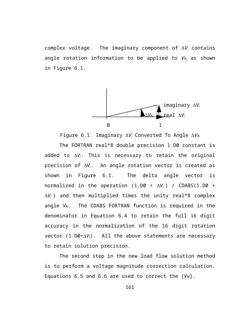
Table 13.8 (FG(x)-FE(x))/FE(x) Error In The PQ Convolution

Probability generation will not be able to serve load PQ per unit error with respect to 1 MW Booth-Baleriaux

58197 0.00000000 0.00000000 0.00000000 -0.00000006 0.00000000 57906 0.00000000 0.00000000 0.00000006 -0.00000006 0.00000000 ...cont... 37828 0.01318914 0.01333044 0.01349173 0.01365492 0.01381955 37537 0.01398659 0.01412272 0.01469016 0.00789680 0.10326142

Table 13.9 Real And Virtual Generator Incremental Load Flows Creating Hi,k Factors

incremental flow monitor ...

1 DBBRN1 575.0 MW TO STUDY AREA iter 0 bus 3380 perr= 575.00 bus 5210 qerr= 1.93 iter 1 bus 4401 perr= 3.52 bus 2398 qerr= 0.51 iter 2 bus 3380 perr= 3.56 bus 3127 qerr= 0.03 iter 3 bus 3380 perr= 0.24 bus 4818 qerr= 0.01 iter 4 bus 3380 perr= 0.05 bus 3304 qerr= 0.00 iter 5 bus 3380 perr= 0.01 bus 3304 qerr= 0.00 iter 6 bus 3380 perr= 0.00 bus 3304 qerr= 0.00

...cont...

9 COA 1811.2 MW TO STUDY AREA iter 0 bus 9079 perr= 42.61 bus 9257 qerr= 20.67 iter 1 bus 9187 perr= 12.35 bus 9075 qerr= 2.85 iter 2 bus 9187 perr= 0.65 bus 9075 qerr= 0.11 iter 3 bus 5915 perr= 0.05 bus 7499 qerr= 0.01 iter 4 bus 9187 perr= 0.02 bus 7499 qerr= 0.00 iter 5 bus 8293 perr= 0.00 bus 7499 qerr= 0.00

...cont...

average weighted scale factor = 0.97 % (avg. percent adjustment) creating GENY.BIN (stores H dist. factors) Gen-line dist fac time= 0h 4m 49s

171

Table 13.10 is a listing of lines in descending order of xminj and xmaxj (the

column listed as PCT) and the largest Hi,m-n generator to load distribution factors

(column listed as DIST). This is the first screening step in deciding which lines to

monitor for overload. Some of the top entries have extremely small probabilities of

~10-80 of being highly overloaded as do most of the lines shown below. Figure 8.1

shows the typical probability of maximum line MW for ERCOT. The actual table

below needs about 500 lines to cover all the ERCOT probabilistic line overloads.

Table 13.10 Lines With Largest Probabilistic MW Overload In Descending Order

MAXIMUM PROBABILISTIC CIRCUIT LOADS WITH ALL LINES IN SERVICE

-------FROM------ -------TO-------- RATG PCT -GENERATION- to -LOAD- DIST 3391 JEWETT N 345 4676 TOMBAL 5 345 717 315.9 LIMEST 5 345 -> HLP .196 32 ROBERTSN 138 3682 MILANO M 138 84 282.3 DANSBY D -> LCRA .105 3391 JEWETT N 345 4676 TOMBAL 5 345 717 -276.0 T H W E8 138 -> TU .198 3380 BIGBRN 345 3391 JEWETT N 345 1072 -241.9 TWIN OAK 345 -> TU .220 241 WHITNEY 138 242 WHITNEY 69.0 32 -235.5 WHITNEY 69.0 -> LCRA .727 ...cont

Table 13.11 shows the results of the zipflow line outages. This step is

performed to develop a set of complex line distribution currents that are used to test

for system separation, used to calculate multiple lines outaged simultaneously, and

used to create new Hi,m-n line distribution factors for the enumerated many lines

outaged cases.

Table 13.11 Single Circuit Line Outages Using 1 Amp Injection Currents

single circuit outage analysis follows...

OUTAGE OF LINE 3001 9187 DECKER 138 -to- 9000 DECKR G124.0 separates the system

OUTAGE OF LINE 3059 9166 BRACK 69.0 -to- 9212 HOLLY 69.0 overloads 3058 9166 BRACK 69.0 -to- 9204 HARRIS 69.0 100. % rating= 108 MW overloads 3077 9204 HARRIS 69.0 -to- 9212 HOLLY 69.0 128. % rating= 108 MW

OUTAGE OF LINE 3077 9204 HARRIS 69.0 -to- 9212 HOLLY 69.0 overloads 3059 9166 BRACK 69.0 -to- 9212 HOLLY 69.0 128. % rating= 108 MW

...cont 94 lines outaged Single line outags tm = 0h 0m 7s

Table 13.12 is similar to Table 13.11, except the CNTG% column includes

the effect of the worst single line outage on increasing the xminj and xmaxj flows on 172

the line. The specific line outaged to create this maximum loading is shown, as well

as the modified largest Hi,m-n line distribution factor for this single line outage case.

This table was initially used as one the of ways to check the correctness of the

process of updating the Hi,m-n factors (column DIST). The PLF now uses this table

information in the final screening process of selecting lines to monitor/not monitor.

Table 13.12 Lines Selected For Monitoring Based First Line Outages Max Flows

LINES SELECTED FOR OUTAGE/MONITORING IN PROBABILISTIC MODELS

-------FROM------ -------TO-------- RATG CNTG% BASE% DIST --OUTAGE-- 7334 MCNEIL 8 138 9079 MCNEILN 138 382 210.3 188.3 .263 7328 9076 9076 MCNEILW 138 9077 MCNEILS 138 430 161.1 126.1 .248 9124 9291 9166 BRACK 69.0 9212 HOLLY 69.0 108 -117.5 -76.0 .144 9204 9212 9129 NORTHLND69.0 9226 KOENIG 69.0 215 117.1 52.2 .231 9212 9243 9129 NORTHLND69.0 9128 NORTHLND 138 220 -114.4 -51.1 .231 9212 9243 ...cont

Table 13.13 Final Selection Of Lines To Monitor And To Outage1

LINES SELECTED FOR OUTAGE/MONITORING IN PROBABILISTIC MODELS

--#- -------FROM------ -------TO-------- OUT MON 1 7202 HICROSS8 138 9147 HICRSMB2 138 0 1 2 7328 AUSTROP8 138 9076 MCNEILW 138 0 1 15 9075 LYTTON 138 9257 PILOT KB 138 1 1 16 9075 LYTTON 138 9267 SLAUGHTR 138 0 1 17 9076 MCNEILW 138 9077 MCNEILS 138 1 1 ...cont

writing line outage file, size in bytes= 40328.0 writing transpose of line outage file

71 lines saved for further analysis Selection of lines tm = 0h 0m 2s

1 Only City of Austin lines are monitored and outaged in this example.

173

The next steps are to calculate the probabilistic line flows F±j(x) and then

perform the heuristic load sheddings. Table 13.14 shows overall probabilities going

into the study. The numbers assume that all lines outside the 71 lines outaged in the

City of Austin system have 100% reliability. All numbers below assume two state

models for both generation and transmission. The double outage line contingencies

plus the total probability space of all generator outages almost completely covers all

the probability space of this problem.

Table 13.14 The Analysis Of Probabilistic Line Loadings And Load Sheddings

BEGIN LARGE SYSTEM ANALYSIS OF ALL GENERATION STATES

number of lines outaged = 16 500 max maximum number of lines out simultaneously = 2 number of generators outaged = 286 350 max number of load areas = 9 total probability of all line states run = 1.0000E+00 total probability of all line states not run = 4.3935E-06 (only COA lines) probability outaged lines are in service = 9.6848E-01 probability outaged generators are in service = 1.5296E-12 probability outaged lines & gens are in servc = 1.4814E-12 maximum number of transmission line states = 6.554e 4 maximum number of generator states = 1.243e 86 maximum number of generator and line states = 8.148e 90

*********************************************** analyzing system for number of circuits out = 0 ***********************************************

line overloaded : 109.0% 7202-9147 HICROSS8 138 - HICRSMB2 138 1 skipped : Prob= 0.32484E-19

line overloaded : 119.4% 7328-9187 AUSTROP8 138 - DECKER 138 3 ratg= 430. MW max loading= 513. MW min loading= -465. MW genr prob=0.000000000004 line prob=0.968479803971 prob ovld=0.000000000004 GENERATOR LOAD AREA DIST FACT LINE MW SHED MW 238 LFAY2 10 COA9 0.190031 14.063 74.003 (offending gen. 237 LFAY1 10 COA9 0.190031 14.552 76.577 and load pair) 137 HSTP2 10 COA9 0.183833 9.559 52.000 136 HSTP1 10 COA9 0.183833 9.559 52.000 235 LGID3 7 LCRA 0.073332 24.200 330.000 233 LGID1 7 LCRA 0.073160 9.877 135.000 234 LGID2 7 LCRA 0.073160 1.529 20.897 ...cont

line overloaded : -108.2% 7328-9187 AUSTROP8 138 - DECKER 138 3 skipped : Prob= 0.00000E+00

174

Table 13.14 (cont)

line overloaded : 188.3% 7334-9079 MCNEIL 8 138 - MCNEILN 138 4 ratg= 382. MW max loading= 719. MW min loading= -612. MW genr prob=0.000000013930 line prob=0.968479803971 prob ovld=0.000000013491 GENERATOR LOAD AREA DIST FACT LINE MW SHED MW 136 HSTP1 9 COA 0.262630 38.869 148.000 (jointly owned) 137 HSTP2 9 COA 0.262630 38.869 148.000 238 LFAY2 9 COA 0.252930 53.273 210.622 237 LFAY1 9 COA 0.252929 55.125 217.948 245 LMFD2 6 WTU * 0.230994 2.079 9.000 (a power sale ) 244 LMFD1 7 LCRA 0.206246 7.012 34.000 246 LMFD3 7 LCRA 0.206035 7.005 34.000 250 LMFL2 7 LCRA 0.147180 2.355 16.000 249 LMFL1 7 LCRA 0.147179 2.355 16.000 231 LBUCH1 7 LCRA 0.119576 1.555 13.000 236 LFRG 7 LCRA 0.115794 49.212 425.000 248 LWRTZ2 7 LCRA 0.113934 2.962 26.000 247 LWRTZ1 7 LCRA 0.113626 2.954 26.000 232 LBUCH2 7 LCRA 0.110317 1.434 13.000 241 LINKS 7 LCRA 0.100991 1.212 12.000 240 LBUCH3 7 LCRA 0.100864 1.311 13.000 152 AGT1 9 COA 0.068239 3.412 50.000 153 AGT2 9 COA 0.068239 3.412 50.000 154 AGT3 9 COA 0.068239 3.412 50.000 155 AGT4 9 COA 0.068239 3.412 50.000 150 ADP1 9 COA 0.067777 15.548 229.400 151 ADP2 9 COA 0.067607 20.012 296.000 57 DALCOA 1 TU 0.062538 5.003 80.000 9 DSAND4 1 TU 0.062413 15.520 248.671 ...cont

line overloaded : -160.1% 7334-9079 MCNEIL 8 138 - MCNEILN 138 4 skipped : Prob= 0.33399E-29

line overloaded : 126.1% 9076-9077 MCNEILW 138 - MCNEILS 138 17 skipped : Prob= 0.41408E-12

line overloaded : 111.3% 9076-9079 MCNEILW 138 - MCNEILN 138 18 skipped : Prob= 0.00000E+00

line overloaded : -109.5% 9076-9079 MCNEILW 138 - MCNEILN 138 18 skipped : Prob= 0.00000E+00 ...cont

*******************DEFINITIONS************************ (defines column headings I3=line number to unload in selected line outage table in the next report) IG=generator number in INPUTB file in which to shed MW J3=firm power contract number in INPUTB file IA=area number in loadflow data in which to shed MW T1=per unit power in line I3 from IG to IA shedding T5=+1 or -1 for forward or reverse line flow in I3 DX=increment of MW unloaded in line I3 T6=the total MW unloaded in I3 T4=MW load shed for this column slice PROB=ENG/DX, average incremental probability ENG=energy in MWH associated with PROB column slice ******************************************************

175

Table 13.14 (cont)

unload line : 7334 MCNEIL 8 138 - 9079 MCNEILN 138 I3 IG J3 IA T1 T5 DX T6 T4 PROB ENG 4 136 0 9 0.26263 1. 33.7 415.7 128.4 0.3227E-08 0.1089E-06 4 136 0 9 0.26263 1. 5.1 420.9 19.6 0.9716E-10 0.4992E-09 (load 4 137 0 9 0.26263 1. 33.7 454.6 128.4 0.1128E-10 0.3806E-09 shedding 4 137 0 9 0.26263 1. 5.1 459.7 19.6 0.9323E-13 0.4790E-12 delta MW 4 238 0 9 0.25293 1. 33.7 493.5 133.4 0.7261E-14 0.2449E-12 increment) line is unloaded: XMW= 399.089 XMWH= 4.046634E-07 from peak: MW= 28298.0 % = 48.6245 (location on x axis) unload line : 7328 AUSTROP8 138 - 9187 DECKER 138 I3 IG J3 IA T1 T5 DX T6 T4 PROB ENG 3 238 0 10 0.19003 1. 8.3 438.4 43.9 0.1825E-11 0.1521E-10 line is unloaded: XMW= 434.186 XMWH= 7.749310E-11 from peak: MW= 2119.00 % = 3.64108 ...cont

*********************************************** analyzing system for number of circuits out = 1 (all single line outages) ***********************************************

------------------------------------------------------------------------------ line state: 2 outage line(s): 9075-9257 LYTTON 138 - PILOT KB 138

line overloaded : -107.2% 7202-9147 HICROSS8 138 - HICRSMB2 138 1 skipped : Prob= 0.00000E+00

line overloaded : 140.9% 7328-9187 AUSTROP8 138 - DECKER 138 3 ratg= 430. MW max loading= 606. MW min loading= -521. MW genr prob=0.000000144006 line prob=0.001940841291 prob ovld=0.000000000279 GENERATOR LOAD AREA DIST FACT LINE MW SHED MW 238 LFAY2 10 COA9 0.225707 16.703 74.002 237 LFAY1 10 COA9 0.225707 17.284 76.576 137 HSTP2 10 COA9 0.218972 11.387 52.000 136 HSTP1 10 COA9 0.218972 11.387 52.000 235 LGID3 7 LCRA 0.068650 22.655 330.000 233 LGID1 7 LCRA 0.068570 9.257 135.000 234 LGID2 7 LCRA 0.068570 9.257 135.000 239 LFAY3 7 LCRA 0.053113 22.042 415.000 275 TGBCR1 7 LCRA * 0.046225 0.139 3.000 145 HUNSP1 1 TU * 0.005376 0.419 78.002 168 CLAR 3 6 WTU * 0.005177 0.124 24.004 ...cont

unload line : 7334 MCNEIL 8 138 - 9079 MCNEILN 138 I3 IG J3 IA T1 T5 DX T6 T4 PROB ENG 4 136 0 9 0.28236 1. 34.0 416.0 120.4 0.1739E-06 0.5911E-05 4 136 0 9 0.28236 1. 7.8 423.8 27.6 0.1172E-07 0.9127E-07 4 137 0 9 0.28236 1. 34.0 457.8 120.4 0.1570E-08 0.5337E-07 4 137 0 9 0.28236 1. 7.8 465.6 27.6 0.3217E-10 0.2506E-09 4 238 0 9 0.27300 1. 34.0 499.6 124.5 0.2568E-11 0.8730E-10 4 238 0 9 0.27300 1. 23.5 523.1 86.1 0.3630E-14 0.8530E-13 line is unloaded: XMW= 399.687 XMWH= 4.162872E-08 from peak: MW= 28298.0 % = 48.6245 ...cont

176

Table 13.14 (cont)

unload line : 7328 AUSTROP8 138 - 9187 DECKER 138 I3 IG J3 IA T1 T5 DX T6 T4 PROB ENG 3 238 0 10 0.22571 1. 16.7 459.7 74.0 0.1539E-07 0.2570E-06 3 237 0 10 0.22571 1. 17.3 477.0 76.6 0.1903E-08 0.3289E-07 3 137 0 10 0.21897 1. 11.4 488.4 52.0 0.2383E-09 0.2714E-08 3 136 0 10 0.21897 1. 11.4 499.8 52.0 0.4373E-10 0.4979E-09 3 235 0 7 0.06865 1. 17.6 517.4 256.0 0.5123E-11 0.9004E-10 3 235 0 7 0.06865 1. 5.1 522.4 74.0 0.5124E-12 0.2603E-11 3 233 0 7 0.06857 1. 9.3 531.7 135.0 0.1465E-12 0.1356E-11 3 234 0 7 0.06857 1. 9.3 541.0 135.0 0.2316E-13 0.2144E-12 3 239 0 7 0.05311 1. 17.6 558.5 330.9 0.1973E-14 0.3467E-13 3 239 0 7 0.05311 1. 4.5 563.0 84.1 0.7848E-16 0.3507E-15 line is unloaded: XMW= 453.723 XMWH= 2.524256E-09 from peak: MW= 2119.00 % = 3.64108

unload line : 9075 LYTTON 138 - 9267 SLAUGHTR 138 I3 IG J3 IA T1 T5 DX T6 T4 PROB ENG 16 237 0 10 0.18128 1. 12.6 447.2 69.4 0.5472E-09 0.6882E-08 line is unloaded: XMW= 440.937 XMWH= 7.368104E-11 from peak: MW= 3493.00 % = 6.00203 ...cont

*********************************************** analyzing system for number of circuits out = 2 (all double line outages) ***********************************************

------------------------------------------------------------------------------ line state: 18 outage line(s): 9075-9257 LYTTON 138 - PILOT KB 138 9076-9077 MCNEILW 138 - MCNEILS 138

line overloaded : -116.3% 7202-9147 HICROSS8 138 - HICRSMB2 138 1 skipped : Prob= 0.00000E+00

line overloaded : 149.0% 7328-9187 AUSTROP8 138 - DECKER 138 3 ratg= 430. MW max loading= 641. MW min loading= -537. MW genr prob=0.000002035328 line prob=0.000003889462 prob ovld=0.000000000008 GENERATOR LOAD AREA DIST FACT LINE MW SHED MW 238 LFAY2 10 COA9 0.247435 18.311 74.002 237 LFAY1 10 COA9 0.247435 18.948 76.577 137 HSTP2 10 COA9 0.240985 12.531 52.000 136 HSTP1 10 COA9 0.240985 12.531 52.000 235 LGID3 7 LCRA 0.066436 21.924 330.000 233 LGID1 7 LCRA 0.066355 8.958 135.000 234 LGID2 7 LCRA 0.066355 8.958 135.000 239 LFAY3 7 LCRA 0.051201 21.248 415.000 275 TGBCR1 7 LCRA * 0.045528 0.137 3.000 145 HUNSP1 1 TU * 0.003782 0.295 78.007 278 TEXASA 8 S.TEX. * 0.003076 0.055 17.998 168 CLAR 3 6 WTU * 0.003033 0.073 24.004 ...cont

unload line : 7328 AUSTROP8 138 - 9187 DECKER 138 I3 IG J3 IA T1 T5 DX T6 T4 PROB ENG 3 238 0 10 0.24743 1. 18.3 448.3 74.0 0.1028E-05 0.1882E-04 line is unloaded: XMW= 439.155 XMWH= 2.958888E-10 from peak: MW= 2119.00 % = 3.64108...cont

177

Table 13.15 is the final output report showing the City of Austin Area 9

LOLP and EUE. Columns 3 and 5 are generation only. Columns 4 and 6 are

transmission LOLP and EUE. The program calculates column 6 first and then

calculates the transmission LOLP from the transmission EUE. The last column to the

right is the ratio of transmission EUE to generation EUE versus % load level. All the

EUE values are for a one hour period.

Table 13.15 Final Reliability Output Report For COA 138 kV System

AREA 9 COA :

LOAD% LOAD-MW LOLP TLOP EUE-MWh TEUE-MWh TOTL-MWh T/G EUE 65.0 1190 0.0000000 0.0000000 0.000000 0.000000 0.000000 11. 66.0 1209 0.0000000 0.0000000 0.000000 0.000000 0.000000 5.7 67.0 1227 0.0000000 0.0000000 0.000000 0.000000 0.000000 2.8 68.0 1245 0.0000000 0.0000000 0.000000 0.000000 0.000000 1.4 69.0 1263 0.0000000 0.0000000 0.000000 0.000000 0.000000 0.74 70.0 1282 0.0000000 0.0000000 0.000000 0.000000 0.000000 0.39 71.0 1300 0.0000000 0.0000000 0.000001 0.000000 0.000001 0.21 72.0 1318 0.0000002 0.0000000 0.000002 0.000000 0.000003 0.11 73.0 1337 0.0000007 0.0000000 0.000010 0.000001 0.000011 6.31E-02 74.0 1355 0.0000027 0.0000000 0.000038 0.000001 0.000039 3.54E-02 75.0 1373 0.0000092 0.0000001 0.000135 0.000003 0.000138 2.01E-02 76.0 1392 0.0000295 0.0000002 0.000456 0.000005 0.000461 1.15E-02 77.0 1410 0.0000892 0.0000003 0.001449 0.000010 0.001458 6.72E-03 78.0 1428 0.0002538 0.0000005 0.004345 0.000017 0.004363 3.97E-03 79.0 1447 0.0006791 0.0000007 0.012297 0.000029 0.012327 2.38E-03 80.0 1465 0.0017096 0.0000011 0.032840 0.000047 0.032887 1.45E-03 81.0 1483 0.0040467 0.0000016 0.082759 0.000074 0.082833 8.92E-04 82.0 1501 0.0090027 0.0000021 0.196834 0.000110 0.196944 5.59E-04 83.0 1520 0.0188139 0.0000028 0.441842 0.000158 0.442000 3.57E-04 84.0 1538 0.0369096 0.0000034 0.936138 0.000217 0.936354 2.31E-04 85.0 1556 0.0679281 0.0000040 1.872245 0.000286 1.872532 1.53E-04 86.0 1575 0.1171925 0.0000043 3.535246 0.000364 3.535610 1.03E-04 87.0 1593 0.1894137 0.0000045 6.304651 0.000446 6.305098 7.08E-05 88.0 1611 0.2866856 0.0000045 10.625719 0.000529 10.626248 4.98E-05 89.0 1630 0.4063490 0.0000044 16.941426 0.000608 16.942034 3.59E-05 90.0 1648 0.5398202 0.0000035 25.592141 0.000676 25.592815 2.64E-05 91.0 1666 0.6735421 0.0000027 36.712231 0.000731 36.712963 1.99E-05 92.0 1685 0.7924315 0.0000022 50.167000 0.000778 50.167778 1.55E-05 93.0 1703 0.8847363 0.0000020 65.568379 0.000814 65.569191 1.24E-05 94.0 1721 0.9459667 0.0000020 82.375847 0.000837 82.376686 1.02E-05 95.0 1740 0.9796151 0.0000009 100.041552 0.000854 100.042404 8.54E-06 96.0 1758 0.9942483 0.0000007 118.134692 0.000867 118.135559 7.34E-06 97.0 1776 0.9989305 0.0000006 136.392331 0.000878 136.393204 6.44E-06 98.0 1794 0.9998996 0.0000011 154.694999 0.000881 154.695877 5.69E-06 99.0 1813 0.9999980 0.0000027 173.005241 0.000929 173.006165 5.37E-06 100.0 1831 1.0000000 0.0000016 191.315913 0.000965 191.316879 5.04E-06 Minimum MWH that can be shed = 0.000459 (if all dist fact =1)

178

Table 13.16 Final Reliability Output Report For COA 69 kV System

AREA 10 COA9 :

LOAD% LOAD-MW LOLP TLOP EUE-MWh TEUE-MWh TOTL-MWh T/G EUE 65.0 373 0.0000000 0.0000000 0.000000 0.000000 0.000000 2.50E+04 66.0 378 0.0000000 0.0000000 0.000000 0.000000 0.000000 7.84E+03 67.0 384 0.0000000 0.0000001 0.000000 0.000001 0.000001 2.50E+03 68.0 390 0.0000000 0.0000001 0.000000 0.000001 0.000001 8.15E+02 69.0 395 0.0000000 0.0000002 0.000000 0.000002 0.000002 2.66E+02 70.0 401 0.0000000 0.0000002 0.000000 0.000003 0.000003 82. 71.0 407 0.0000000 0.0000002 0.000000 0.000004 0.000005 24. 72.0 413 0.0000002 0.0000002 0.000001 0.000006 0.000006 7.2 73.0 418 0.0000007 0.0000003 0.000003 0.000007 0.000010 2.2 74.0 424 0.0000027 0.0000004 0.000012 0.000009 0.000021 0.76 75.0 430 0.0000092 0.0000007 0.000042 0.000012 0.000055 0.29 76.0 436 0.0000295 0.0000009 0.000143 0.000017 0.000160 0.12 77.0 441 0.0000892 0.0000009 0.000453 0.000022 0.000476 4.95E-02 78.0 447 0.0002538 0.0000009 0.001360 0.000028 0.001388 2.03E-02 79.0 453 0.0006791 0.0000009 0.003849 0.000033 0.003882 8.56E-03 80.0 458 0.0017096 0.0000010 0.010278 0.000039 0.010317 3.75E-03 81.0 464 0.0040467 0.0000015 0.025902 0.000046 0.025948 1.79E-03 82.0 470 0.0090027 0.0000023 0.061604 0.000059 0.061662 9.50E-04 83.0 476 0.0188139 0.0000026 0.138285 0.000073 0.138358 5.29E-04 84.0 481 0.0369096 0.0000027 0.292987 0.000088 0.293076 3.02E-04 85.0 487 0.0679281 0.0000028 0.585965 0.000104 0.586069 1.78E-04 86.0 493 0.1171925 0.0000031 1.106443 0.000121 1.106564 1.10E-04 87.0 499 0.1894137 0.0000043 1.973196 0.000144 1.973340 7.31E-05 88.0 504 0.2866856 0.0000056 3.325581 0.000175 3.325756 5.26E-05 89.0 510 0.4063490 0.0000065 5.302237 0.000211 5.302448 3.98E-05 90.0 516 0.5398202 0.0000065 8.009692 0.000248 8.009940 3.10E-05 91.0 522 0.6735421 0.0000066 11.489998 0.000286 11.490284 2.49E-05 92.0 527 0.7924315 0.0000067 15.701000 0.000324 15.701324 2.06E-05 93.0 533 0.8847363 0.0000074 20.521242 0.000365 20.521606 1.78E-05 94.0 539 0.9459667 0.0000091 25.781554 0.000415 25.781969 1.61E-05 95.0 544 0.9796151 0.0000110 31.310472 0.000476 31.310947 1.52E-05 96.0 550 0.9942483 0.0000110 36.973166 0.000539 36.973705 1.46E-05 97.0 556 0.9989305 0.0000110 42.687345 0.000602 42.687946 1.41E-05 98.0 562 0.9998996 0.0000106 48.415616 0.000664 48.416279 1.37E-05 99.0 567 0.9999980 0.0000084 54.146258 0.000716 54.146973 1.32E-05 100.0 573 1.0000000 0.0000023 59.877035 0.000740 59.877773 1.24E-05 Minimum MWH that can be shed = 0.000317

Notice that the transmission LOLP need not be monotone decreasing.

However, the sum of the transmission LOLP and the generation LOLP must be

monotone decreasing. 100% load means a load level equal to 100% of owned

capacity by the area listed. In this example, the City of Austin transmission system

appears to be very reliable. The minimum MWH that can be shed assumes all H’s

are exactly one.

179

Table 13.17 Final Reliability Output Report For The Total System TOTAL SYSTEM: (only has the COA line outages)

LOAD% LOAD-MW LOLP TLOP EUE-MWh TEUE-MWh TOTL-MWh T/G EUE 65.0 37828 0.0000000 0.0000000 0.000000 0.000000 0.000000 8.09E-05 66.0 38410 0.0000000 0.0000000 0.000000 0.000000 0.000000 4.67E-05 67.0 38992 0.0000000 0.0000000 0.000000 0.000000 0.000000 8.75E-05 68.0 39574 0.0000000 0.0000000 0.000000 0.000000 0.000000 1.11E-04 69.0 40156 0.0000000 0.0000000 0.000001 0.000000 0.000001 9.57E-05 70.0 40738 0.0000000 0.0000000 0.000004 0.000000 0.000004 7.21E-05 71.0 41320 0.0000000 0.0000000 0.000018 0.000000 0.000018 5.51E-05 72.0 41902 0.0000002 0.0000000 0.000079 0.000000 0.000079 3.98E-05 73.0 42484 0.0000007 0.0000000 0.000317 0.000000 0.000317 2.90E-05 74.0 43066 0.0000027 0.0000000 0.001202 0.000000 0.001202 2.13E-05 75.0 43648 0.0000092 0.0000000 0.004296 0.000000 0.004296 1.59E-05 76.0 44230 0.0000295 0.0000000 0.014482 0.000000 0.014482 1.20E-05 77.0 44812 0.0000892 0.0000000 0.046045 0.000000 0.046046 9.15E-06 78.0 45394 0.0002538 0.0000000 0.138110 0.000001 0.138111 7.05E-06 79.0 45976 0.0006791 0.0000000 0.390850 0.000002 0.390852 5.49E-06 80.0 46558 0.0017096 0.0000000 1.043745 0.000005 1.043750 4.32E-06 81.0 47140 0.0040467 0.0000000 2.630346 0.000009 2.630355 3.43E-06 82.0 47722 0.0090027 0.0000000 6.255971 0.000017 6.255988 2.75E-06 83.0 48304 0.0188139 0.0000000 14.043084 0.000031 14.043116 2.22E-06 84.0 48885 0.0369096 0.0000000 29.753304 0.000054 29.753357 1.81E-06 85.0 49467 0.0679281 0.0000001 59.505642 0.000088 59.505730 1.48E-06 86.0 50049 0.1171925 0.0000001 112.360863 0.000137 112.361000 1.22E-06 87.0 50631 0.1894137 0.0000001 200.380966 0.000202 200.381165 1.01E-06 88.0 51213 0.2866856 0.0000001 337.717621 0.000282 337.717896 8.35E-07 89.0 51795 0.4063490 0.0000002 538.449951 0.000375 538.450317 6.96E-07 90.0 52377 0.5398202 0.0000002 813.395935 0.000472 813.396423 5.81E-07 91.0 52959 0.6735421 0.0000002 1166.826172 0.000568 1166.826782 4.86E-07 92.0 53541 0.7924315 0.0000001 1594.459595 0.000653 1594.460205 4.10E-07 93.0 54123 0.8847363 0.0000001 2083.962158 0.000723 2083.962891 3.47E-07 94.0 54705 0.9459667 0.0000001 2618.154541 0.000775 2618.155273 2.96E-07 95.0 55287 0.9796151 0.0000001 3179.624268 0.000813 3179.625000 2.56E-07 96.0 55869 0.9942483 0.0000000 3754.679199 0.000839 3754.679932 2.23E-07 97.0 56451 0.9989305 0.0000000 4334.962402 0.000863 4334.963379 1.99E-07 98.0 57033 0.9998996 0.0000002 4916.676758 0.000934 4916.677734 1.90E-07 99.0 57615 0.9999980 0.0000006 5498.631836 0.001214 5498.632813 2.21E-07 100.0 58197 1.0000000 0.0000010 6080.600586 0.001704 6080.602051 2.80E-07 Minimum MWH that can be shed = 0.000776 : : : : : : Installed : : : : Ratio of unserved energies Generation : : : : Transmission to Generation : : : : Probability of not : : Additional unserved MWH due serving load at : : to transmission constraints system peak hour : : : : Probability transmission Unserved MWH during the peak load hour will be a bottleneck due only to insufficient generation

large system analysis completed # xmissn states examined = 137 Prob of system separation = 0.1556E-04 Prob of untested states = 0.4255E-05 Prob of all states tested = 0.999996 Large System run time 0h 28m 14s Total run time 0h 34m 27s (excellent for ~1.E90 outage configs)

180

Chapter 14

Conclusions and Recommendations

A new model is presented in this dissertation for calculating generation

reliability with transmission constraints in large electric power systems. The large

networks today are highly interconnected through high voltage transmission lines to

reduce costs and improve reliability. The sharing of generation reserves greatly

improves power supply reliability. Economy energy transfers reduce operating costs.

By design, today’s systems have a high degree of freedom to dispatch scheduled

generation from any generator to any load area. This high degree of interconnectivity

also allows an extremely large number of unscheduled random generator outage

configurations to be possible. A network with 300 generators (such as the ERCOT

system) has ~1090 configurations in which the generators can randomly fail. Many of

these configurations will cause transmission line flows exceeding line capacities. The

chance that any one of these configurations will occur is very small, but collectively,

their effect on total system reliability is significant and measurable.

The PLF model presented in this dissertation is new because a convolution

solution approach allows the complete set of generation outage configurations to be

modeled for every line outage configuration. Computation time is excellent. The

ERCOT system example presented in Chapter 13 modeled ~1090 generation outage

configurations for each of the 137 COA area line outage configurations with a total

computation time of 35 minutes on a 75 MHz Pentium personal computer. The PLF

model is the first in the industry to include the complete set of probabilistic line flows

due to all generation outage configurations as a normal part of the planning analysis

of the transmission system.

181

All the other composite generation-transmission system models being

marketed use enumeration techniques to model both the generation and transmission

outage configurations. Enumeration of transmission outage configurations can be

used to cover a majority of the transmission failure events probability space because

the outage rates of lines are very small. However, the outage rates of generators are

not small. In a large system several generators will be outaged at any one time. This

creates a computer run-time problem for solution approaches using enumeration of

generation outages for large systems. Execution times of days and weeks are

common for a single case, and results are always questionable. For this reason, the

composite generation-transmission models have not been widely accepted by the

engineers planning and operating the large systems.

The convolution techniques used in this dissertation overcome the problem of

extremely long computer run times associated with the modeling of generation outage

configurations. The model presented in this dissertation has the following desirable

features.

· Larger networks can be modeled with this PLF model than the best of the others.

· A full transmission network is represented, eliminating the need for an

equivalent.

· All generation outage states are modeled exhaustively (completely).

· Transmission outages are enumerated quickly with an efficient line outage model.

· Solution times are in hours instead of days (needed by other computer programs).

· Loss of load due to generation outages is uniform throughout the network.

· Loss of load due to transmission constraints is assigned to specific lines,

generators, and loads in a near optimal manner.

182

The PLF model is not a complete model in the sense that no further

improvements are necessary. The author’s recommendations for continuing work

with this model are listed below.

· Incorporate the three state generator outage model in the PLF program.

· Add to the PLF model the EUE load shed MWh due to system separations.

· Further review the theory and operation of the load shedding heuristic to see if

improvements in its performance can be made.

· Investigate the feasibility of adding the frequency of load sheddings as a part of

the convolution process presented in this dissertation.

· Increase the PLF load flow model from its present 5000 buses to 50000 buses for

the purpose of testing the reliability of the eastern and western electric power

systems.

· Conduct an analysis of the generation and transmission reliability of every area in

ERCOT for the purpose of determining how well the City of Austin compares

with the other areas in overall reliability and to identify those components within

the COA system that are causing any reliability deficiencies.

The author believes the methods presented in this dissertation represent

important advancements to the present state of knowledge concerning the assessment

of power system reliability. At this time, the PLF model is unique in the electric

utility industry.

183

Appendix ADerivations

Derivation of Equation 3.11Given any finite continuous, discontinuous, or discrete density function f(x) or

continuous or discontinuous cumulative distribution F(x), the convolution of a very

small width rectangular block function of width Dx and heighth 1/Dx located at x = a

with the f(x) or F(x) function causes a shift of the f(x) or F(x) function as shown in

Figure A.1. For finite Dx, the shift is aproximate. In the limit as Dx®0, the shift of

f(x) to the right by a is an exact process.

1/Dx

f(x) » f(x-a)

Dx

0 a 0

Figure A.1 Convolution of an Impulse Function With f(x)

This can be written as an impulse function d(x-a) replacing the rectangular section.

Convolving the impulse function with f(x) produces

ó +¥

f(x)+ = ô f(y)d(x-y-a) dy = f(x-a) . (A.1)õ-¥

The f(x)+ is the function after convolution. The original f(x) function before

convolution is simply shifted to the right by a as a result of the convolution.

184

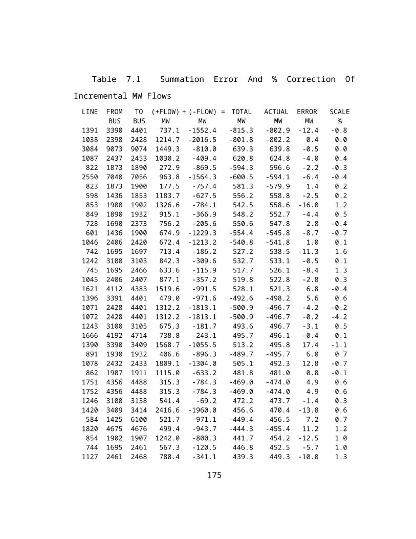
The three state generator model (Table 3.1) can be written as an impulse

function. For any generator k, let the state probabilities be pu = 1-DFORk-FORk for

the up state, pd = DFORk for the derated state, and po = FORk for the outaged state.

The convolution of these generator k states into the cumulative distribution F(x) is

given in Equation A.2 as

ó +¥

F(x)+ = ô F(y)[pud(x-y) + pdd(x-y-Dk) + pod(x-y-Ck)]dy . (A.2)õ-¥

Evaluating Equation A.2 produces

F(x)+ = puF(x) + pdF(x-Dk) + poF(x-Ck) . (A.3)

Equation A.3 is equivalent to Equation 3.11 which completes the derivation.

185

Derivation of Equation 3.13A simple notation is used to develop the piecewise quadratic function shown

in Equation 3.13. The resulting equation from the simpler notation derivation is

shown to be equivalent to Equation 3.13. Figure A.2 shows a quadratic curve fit of

any three consecutive evenly spaced points on F(x) with values F-1 , F0 , and F+1 .

The discrete points are located at points x=-r, x=0, and x=r, respectively, where

-1 £ r < 1. A, B, and C are dummy coefficients in the quadratic equation

Fr=Ar2 + B r + C . Fr provides a smooth function interpolation of the discrete points.

F-1

F0

F+1

local range r : -1 0 +1

Figure A.2 Piecewise Quadratic Spline Fr

Solving for coefficients A, B, and C:

1. F-1 = A -B +C

2. F0 = C

3. F+1 = A +B +C (A.4)

Then C = F0 (A.5)

Adding 1 and 3 F-1 + F+1 = 2A + 2F0 (A.6)

Solving for A A = «F-1 - F0 + «F+1 (A.7)

186

Subtracting 1 from 3 F+1 - F-1 = 2B (A.8)

Solving for B B = «F+1 - «F-1 (A.9)

Inserting the A, B, C coefficients into the original equation

Fr = («F-1 - F0 + «F+1)r2 + («F+1 - «F-1)r + F0 (A.10)

Collecting common F terms gives

Fr = («r2 - «r)F-1 + (1 - r2)F0 + («r2 + «r)F+1 (A.11)

Equation A.11 is the same as Equation 3.13 which completes the derivation.

187

Derivation of Equation 3.14The convolution process uses an interpolation of Fr between the left most and

central points as shown in Figure A.3. The shift of Fr in the convolution process is

done by calculating the interpolated function values for D MW and C MW (shown

below) for the derated and full outaged capacity states respectively. This is most

convenient if the direction of r is reversed from that shown in Figure A.2. So Figure

A.3 shows positive interpolation r to the left of discrete point Fi-j. New point Fi+

value is calculated from the original function to the left by C MW. The C and D MW

consists of a number of integer steps j plus a fractional part of a step r. The j and r

are calculated from the equation C = h(jc+rc) where h is the grid increment MW step

size. The derated state is shifted by D = h(jd+rd) MW.

F i-j-1 C or D Fi+

Fi-j

Fi-j+1

r

j

local range r : +1 0 -1

Figure A.3 Piecewise Quadratic Interpolation

Inserting negative r into Equation A.11 produces

Fr = («r2 + «r)F-1 + (1 - r2)F0 + («r2 - «r)F+1 (A.12)

188

Let the generator state probabilities be pu, pd, and po for the up, derated, and

outaged states. For any new x = ih discrete point on the F(ih)+ function, the

convolution Equation A.3 becomes

Fi+ = puFi + pdF(ih-D) + poF(ih-C) . (A.13)

Inserting the j and r terms for the C and D MW shifts gives

Fi+ = puFi + pdF[ih-(jd+rd)h] + poF[ih-(jc+rc)h] . (A.14)

Expanding the shifted terms in the above equation using Equation A.12 produces

Fi+ = puFi

+ pd[(«rd2 + «rd)Fi-jd-1 + (1 - rd

2)Fi-jd + («rd2 - «rd)Fi-jd+1]

+ po[(«rc2 + «rc)Fi-jc-1 + (1 - rc

2)Fi-jc + («rc2 - «rc)Fi-jc+1]

for integers jc ³ 0 and jd ³ 0 and reals 0 £ rc £ 1 and 0 £ rd £ 1 .

(A.15)

Equation B.15 is equivalent to Equation 3.14, which completes the derivation.

189

Appendix BFortran Subroutines

Sparse Matrix SolverC 'MATRIX SYMMETRICAL SOLUTION' TECHNIQUE FOR N SPARSE EQUATIONS ASC DESCRIBED BY K. ZOLLENKOPF IN HIS PAPER 'BASIC COMPUTATIONAL TECHNIQUES'C APPEARING IN THE BOOK TITLED 'LARGE SPARSE SETS OF LINEAR EQUATIONS' ANDC EDITED BY J. K. REID. ACADEMIC PRESS, 1971, PAGES 75-96.CC THE USER IS RESPONSIBLE FOR DIMENSIONING THE FOLLOWING ARRAYS IN THEC MAIN PROGRAM: LCOL(N),NOZE(N),NSEQ(N),V(N),ITAG(M),LNXT(M),CE(M)C WHERE N IS THE NUMBER OF EQUATIONS AND M IS ALWAYS GREATER THAN THEC NUMBER OF NONZERO ELEMENTS IN THE MATRIX. M REQUIREMENTS VARYC DEPENDING ON THE NATURE OF THE SPARSITY.CC THEN TO USE IT:C CALL MATSS(0) FOR SIMULATION, ORDERING, AND REDUCTIONC CALL MATSS(1) FOR THE SOLUTION THAT IS RETURNED IN ARRAY V.C THE INPUT DRIVING VECTORS WERE ENTERED IN V ALSO.C NOTE THAT (0) NEED BE PERFORMED ONLY ONCE FOR ANY NO. OF SOLUTIONSC THE INITIAL VALUE FOR M FOR (0) SHOULD BE THE USER'S ARRAY SIZE INC THE MAIN PROGRAM DIMENSION STATEMENT. AFTER THE FIRST PASS THROUGHC MATSS, THE VALUE OF M IS THE AMOUNT ACTUALLY USED.C THE USER MUST ALSO PREPARE THE FOLLOWING ARRAYS:C V CONTAINS THE INDEPENDENT DRIVING VECTORSC CE CONTAINS THE NONZERO MATRIX ELEMENTS WHILE A SWEEP ISC MADE FROM LEFT TO RIGHT THROUGH EACH EQUATIONC ITAG RECORDS THE COLUMN POSITION OF EACH CE ELEMENTC NOZE RECORDS THE NUMBER OF CE ELEMENTS PER EQUATIONCSUBROUTINE MATSS(ISOL)C ISOL=0 TO BUILD AND FACTOR THE SPARSE MATRIXESC ISOL=1 TO SOLVE THE MATRIX, AND CAN BE REPEATED ANY NUMBER OF TIMES COMPLEX V(1000),CE(5000),CD,CF INTEGER NOZE(1000),NSEQ(1000),LCOL(1000),ITAG(5000),LNXT(5000) COMMON N,M,MAXM,NOZE,NSEQ,LCOL,ITAG,LNXT,V,CE IF(ISOL.EQ.1) GOTO 1C DEFINE THE MAXIMUM ARRAY SIZE OF CE, ITAG, AND LNXT M=5000 MAXM=0C BUILD LNXT ARRAY DO 2 I=1,M 2 LNXT(I)=I+1 J=0 DO 3 I=1,N J=J+NOZE(I) 3 LNXT(J)=0C SET LAST LNXT AND UNUSED CE TO ZERO LNXT(M)=0 LF=J+1 DO 4 J=LF,M 4 CE(J)=0.

190

C BUILD LCOL ARRAY J=1 DO 5 I=1,N LCOL(I)=J 5 J=J+NOZE(I)C BUILD NSEQ ARRAY DO 6 I=1,N 6 NSEQ(I)=IC BEGIN SIMULATION AND ORDERING, REFERENCE PAGE 89 N1=N-1 DO 17 J=1,N1 K=NSEQ(J) MIN=NOZE(K) M=J L=J+1 DO 16 I=L,N K=NSEQ(I) IF(NOZE(K).GE.MIN) GOTO 16 MIN=NOZE(K) M=I 16 CONTINUE KP=NSEQ(M) NSEQ(M)=NSEQ(J) NSEQ(J)=KP LK=LCOL(KP) 15 K=ITAG(LK) IF(K.EQ.KP) GOTO 11 LA=0 LI=LCOL(KP) IP=ITAG(LI) L=LCOL(K) I=ITAG(L) 10 IF(I-IP) 7,8,9 7 LA=L L=LNXT(L) I=N+1 IF(L.GT.0) I=ITAG(L) GOTO 10 8 IF(I.EQ.KP) GOTO 12 LA=L L=LNXT(L) GOTO 13 12 LN=LNXT(L) IF(LA.GT.0) THEN LNXT(LA)=LN ELSE LCOL(K)=LN ENDIF LNXT(L)=LF LF=L IF(LF.GT.MAXM) MAXM=LF CE(L)=0. NOZE(K)=NOZE(K)-1 L=LN 13 I=N+1 IF(L.GT.0) I=ITAG(L)

191

GOTO 14 9 IF(LF.LE.0) THEN WRITE(*,*) 'MATRIX SPACE IS EXHAUSTED' STOP ENDIF LN=LF IF(LA.GT.0) THEN LNXT(LA)=LN ELSE LCOL(K)=LN ENDIF LF=LNXT(LN) LNXT(LN)=L ITAG(LN)=IP NOZE(K)=NOZE(K)+1 LA=LN 14 LI=LNXT(LI) IF(LI.GT.0) THEN IP=ITAG(LI) GOTO 10 ENDIF 11 LK=LNXT(LK) IF(LK.GT.0) GOTO 15 17 CONTINUEC BEGIN REDUCTION, REFERENCE PAGE 90 DO 18 J=1,N KP=NSEQ(J) LK=LCOL(KP) LP=LF 19 IF(LP.LE.0) THEN WRITE(*,*)'MATRIX SPACE IS EXHAUSTED' STOP ENDIF K=ITAG(LK) IF(K.EQ.KP) THEN CD=1./CE(LK) CE(LK)=CD ELSE CE(LP)=CE(LK) ENDIF LK=LNXT(LK) IF(LK.GT.0) THEN LP=LNXT(LP) GOTO 19 ENDIF LK=LCOL(KP) 20 K=ITAG(LK) IF(K.EQ.KP) GOTO 25 CF=CD*CE(LK) CE(LK)=-CF LP=LF LI=LCOL(KP) IP=ITAG(LI) L=LCOL(K) I=ITAG(L) 26 IF(I-IP) 22,23,24

192

22 L=LNXT(L) IF(L.LE.0) GOTO 25 I=ITAG(L) GOTO 26 23 CE(L)=CE(L)-CF*CE(LP) L=LNXT(L) IF(L.LE.0) GOTO 25 I=ITAG(L) 24 LI=LNXT(LI) IF(LI.LE.0) GOTO 25 IP=ITAG(LI) LP=LNXT(LP) GOTO 26 25 LK=LNXT(LK) IF(LK.GT.0) GOTO 20 18 CONTINUE RETURNC BEGIN DIRECT SOLUTION, REFERENCE PAGE 91 1 M=0 DO 27 J=1,N K=NSEQ(J) CF=V(K) V(K)=0. L=LCOL(K) 28 I=ITAG(L) V(I)=V(I)+CE(L)*CF L=LNXT(L) M=M+1 IF(L.GT.0) GOTO 28 27 CONTINUE J=N 29 IF(J.LE.1) RETURN J=J-1 K=NSEQ(J) CD=V(K) L=LCOL(K) 30 I=ITAG(L) IF(I.NE.K) CD=CD+CE(L)*V(I) L=LNXT(L) IF(L.GT.0) GOTO 30 V(K)=CD GOTO 29 END

193

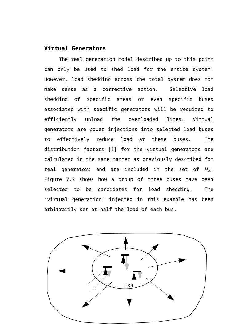
PQ Convolution Routine SUBROUTINE CONVOL(C,Q,X1,X2,K) PARAMETER (MPQ=360)* Convolution of C MW into F(i=x/H+B), P state is scaled but not shifted,* down state (prob=Q) is scaled and shifted, +C is right, -C is left.* X1 and X2 are min and max range of X (real number line) respectively* To perform a simple two state convolution set K=0* To perform multi-state convolution, the first call of convol K=1,* then subsequent calls will have K=2, and the last call has K=3.* For K=0 the convolution of P and Q states is completed in this one CALL.* For K=1 and 2, Q adds on to F(i), the Q, C shifted states; C can be + or -.* For K=3, the P*F3(i) nonshifted terms are also added as a final step. COMMON /EIGHT/F(MPQ),F3(MPQ+5),H,B P=1.-Q IF(K.LE.1) THEN DO 8 I=1,MPQ F3(I)=F(I) F(I)=0. 8 CONTINUE F3(MPQ+1)=X1 F3(MPQ+2)=X2 F3(MPQ+3)=0. F3(MPQ+4)=0. F3(MPQ+5)=Q ELSE F3(MPQ+5)=F3(MPQ+5)+Q P=1.-F3(MPQ+5) ENDIF IF(C.LT.F3(MPQ+3)) F3(MPQ+3)=C IF(C.GT.F3(MPQ+4)) F3(MPQ+4)=C X1=F3(MPQ+1)+F3(MPQ+3) X2=F3(MPQ+2)+F3(MPQ+4) N2=X2/H+B+2 IF(N2.GT.MPQ) N2=MPQ R=C/H J=R R=R-J IF(C.LT.0.) THEN J=-J R=-R R=1-R ENDIF A0=Q*R*(R+1)/2 A1=Q*(1-R**2) A2=Q*R*(R-1)/2 IF(C.LT.0.) GOTO 4* finish the convolution of positive C J=N2-J IF(J+1.GT.MPQ) THEN Y1=0. GOTO 2 ENDIF IF(J+1.LT.1) THEN

194

Y1=1. GOTO 2 ENDIF Y1=F3(J+1) 2 IF(J.GT.MPQ) THEN Y0=0. GOTO 3 ENDIF IF(J.LT.1) THEN Y0=1. GOTO 3 ENDIF Y0=F3(J) 3 DO 1 I=N2,1,-1 Y2=Y1 Y1=Y0 J=J-1 IF(J.GT.MPQ) THEN Y0=0. GOTO 9 ENDIF IF(J.LT.1) THEN Y0=1. GOTO 9 ENDIF Y0=F3(J) 9 F(I) = A2*Y2 + A1*Y1 + A0*Y0 + F(I) IF(K.EQ.0.OR.K.EQ.3) F(I) = F(I) + P*F3(I) 1 CONTINUE RETURN* finish the convolution of negative C 4 J=1+J Y1=0. IF(J.LE.MPQ) Y1=F3(J) J=J+1 Y2=0. IF(J.LE.MPQ) Y2=F3(J) DO 7 I=1,N2 Y0=Y1 Y1=Y2 J=J+1 Y2=0. IF(J.LE.MPQ) Y2=F3(J) F(I) = A2*Y2 + A1*Y1 + A0*Y0 + F(I) IF(K.EQ.0.OR.K.EQ.3) F(I) = F(I) + P*F3(I) 7 CONTINUE RETURN END

195

PQ Evaluate F(x)* Evaluate F(x) at point x=D FUNCTION FPQ(D) PARAMETER (MPQ=360) COMMON /EIGHT/F(MPQ),F3(MPQ+5),H,B R=D/H+B J=R R=R-J IF(R.GT.0.) THEN J=J+1 R=1-R ELSE R=-R ENDIF IF(J.LT.MPQ) THEN Y0=1. Y1=1. Y2=1. IF(J-1.GE.1) Y0=F(J-1) IF(J. GE.1) Y1=F(J) IF(J+1.GE.1) Y2=F(J+1) ELSE Y0=0. Y1=0. Y2=0. IF(J-1.LE.MPQ) Y0=F(J-1) IF(J .LE.MPQ) Y1=F(J) IF(J+1.LE.MPQ) Y2=F(J+1) ENDIF A0=R*(R+1.)/2. A1=1-R**2 A2=R*(R-1.)/2. FPQ = A0*Y0 + A1*Y1 + A2*Y2 RETURN END

196

PQ EUE Routine* Integration of F(x) from D1<x<D2; D1 and D2 can be any real number 0<D1<D2 FUNCTION AINTGR(D1,D2) PARAMETER (MPQ=360) COMMON /EIGHT/F(MPQ),F3(MPQ+5),H,B IF(D1.LT.0.OR.D2.LT.D1) THEN AINTGR=0. RETURN ENDIF D=D2 ID=2 2 R=D/H+B J=R R=R-J J=J+1 R=1.-R AINTGR=0. IF(J.LE.MPQ) THEN DO 1 I=MPQ,J,-1 IF(I.GT.0) THEN AINTGR=AINTGR+F(I) ELSE AINTGR=AINTGR+1. ENDIF 1 CONTINUE ENDIF IF(J.LT.MPQ) THEN Y0=1. Y1=1. Y2=1. IF(J-1.GE.1) Y0=F(J-1) IF(J. GE.1) Y1=F(J) IF(J+1.GE.1) Y2=F(J+1) ELSE Y0=0. Y1=0. Y2=0. IF(J-1.LE.MPQ) Y0=F(J-1) IF(J .LE.MPQ) Y1=F(J) IF(J+1.LE.MPQ) Y2=F(J+1) ENDIF AINTGR = Y2/12. -Y1*7/12. +R**3/6.*(Y0 -2*Y1 +Y2) + & R**2/4.*(Y0 -Y2) +R*Y1 + AINTGR AINTGR=AINTGR * H IF(ID.EQ.2) THEN A2=AINTGR D=D1 ID=1 GOTO 2 ENDIF IF(AINTGR.LT.A2.OR.H.LT.0.) THEN AINTGR=0. RETURN ENDIF AINTGR=AINTGR-A2 RETURN END

197

Bibliography1

Probabilistic Composite Generation-Transmission Models

[1] E. Preston, M. Grady, and M. Baughman, A New Planning Model For Assessing The Effects Of Transmission Capacity Constraints On The Reliability Of Generation Supply For Large Nonequivalenced Electric Networks, IEEE/PES T&D Meeting, Los Angeles, CA, September 1996.

[2] IEEE Task Force, IEEE Reliability Test System - 1996, IEEE/PES Winter Meeting, Baltimore, MD, Paper 96 WM 326-9 PWRS, Jan. 1996.

[3] C. Singh, J. Mitra, Composite System Reliability Evaluation Using State Space Pruning, IEEE/PES Winter Meeting, Baltimore, MD, Paper 96 WM 315-2 PWRS, Jan. 1996.

[4] F. Sener, E. Greene, Top Three Technical Problems - A Survey Report of the Long Range System Planning Working Group, System Planning Subcommittee, Engineering Committee, IEEE PES, IEEE/PES Winter Meeting, Baltimore, MD, Paper 96 WM 271-7 PWRS, Jan. 1996.

[5] J. Mitra, C. Singh, Incorporating the DC Load Flow in the Decomposition-Simulation Method of Multi-Area Reliability Evaluation, IEEE/PES Summer Meeting, Portland, OR, Paper 95 SM 511-6 PWRS, July 1995.

[6] F. Xia, A. Meliopoulos, A Method For Probabilistic Simultaneous Transfer Capability Analysis, IEEE/PES Summer Meeting, Portland, OR, Paper 95 SM 514-0 PWRS, July 1995.

[7] A. Sankarakrishnan, R. Billington, Sequential Monte Carlo Simulation For Composite Power System Reliability Analysis With Time Varying Loads, IEEE Trans. on PWRS, Vol. 10, No. 3, Aug. 1995, pp. 1540-1545.

1 Shown in reverse chronological order by topic.

198

[8] E. Neudorf, D. Kiguel, G. Hamoud, B. Porretta, W. Stephenson, R. Sparks, D. Logan, M. Bhavaraju, R. Billington, D. Garrison, Cost-Benefit Analysis of Power System Reliability: Two Utility Case Studies, Trans. on PWRS, Vol. 10, No. 3, Aug. 1995, pp. 1667-1675.

[9] R. Billington, G. Lian, Composite Power System Health Analysis Using A Security Constrained Adequacy Evaluation Procedure, IEEE Trans. on PWRS, Vol. 9, No. 2, May 1994, pp. 936-941.

[10] R. Allen, R. Billington, A. Breipohl, C. Grigg, Bibliography On The Application Of Probability Methods In Power System Reliability Evaluation 1987-1991, IEEE Trans. on PWRS, Vol. 9, No. 1, Feb. 1994, pp. 41-49.

[11] R. Billington, W. Li, A System State Transition Sampling Method For Composite System Reliability Evaluation, IEEE Trans. on PWRS, Vol. 8, No. 3, Aug. 1993, pp. 761-767.

[12] R. Billington, F. Gbeddy, Effects Of Non-Utility Generators On Composite System Adequacy Evaluation, IEEE Trans. on PWRS, Vol. 8, No. 3, Aug. 1993, pp. 771-777.

[13] A. Cook, I. Rose, A Monte-Carlo Technique For Computing The Benefits Arising From The Interconnection Of Power Systems, IEEE Trans. on PWRS, Vol. 8, No. 3, Aug. 1993, pp. 873-878.

[14] A. Melo, M. Pereira, A. Silva, A Conditional Probability Approach To The Calculation Of Frequency And Duration Indices In Composite Reliability Evaluation, IEEE Trans. on PWRS, Vol. 8, No. 3, Aug. 1993, pp. 1118-1125.

[15] L. Wenyuan, R. Billington, A Minimum Cost Assessment Method For Composite Generation and Transmission System Expansion Planning, Trans. on PWRS, Vol. 8, No. 2, May 1993, pp. 628-635.

[16] Z. Deng, C. Singh, A New Approach To Reliability Evaluation Of Interconnected Power Systems Including Planned Outages And Frequency Calculations, IEEE Trans. on PWRS, Vol. 7, No. 2, May 1992, pp. 734-743.

[17] M. Pereira, L. Pinto, A New Computational Tool For Composite Reliability Evaluation, IEEE Trans. on PWRS, Vol. 7, No. 1, Feb. 1992, pp. 258-264.

199

[18] M. Pereira, M. Maceira, G. Oliveira, L. Pinto, Combining Analytical Models And Monte-Carlo Techniques In Probabilistic Power System Analysis, IEEE Trans. on PWRS, Vol. 7, No. 1, Feb. 1992, pp. 265-272.

[19] A. Sanghvi, N. Balu, M. Lauby, Power System Reliability Planning Practices In North America, IEEE Trans. on PWRS, Vol. 6, No. 4, Nov. 1991, pp. 1485-1492.

[20] M. El-Hawary, G. Mbamalu, A Comparison Of Probabilistic Perturbations And Deterministic Based Optimal Power Flow Solutions, IEEE Trans. on PWRS, Vol. 6, No. 3, Aug. 1991, pp. 1099-1105.

[21] R. Billington, J. Oteng-Adjei, Utilization Of Interrupted Energy Assessment Rates In Generation And Transmission System Planning, IEEE Trans. on PWRS, Vol. 6, No. 3, Aug. 1991, pp. 1245-1253.

[22] G. Haringa, G. Jordan, L. Garver, Application of Monte Carlo Simulation to Multi-Area Reliability Evaluations, IEEE Computer Applications in Power, Vol. 4, No. 1, Jan. 1991, pp. 21-25.

[23] Tutorial, Reliability Assessment of Composite Generation and Transmission Systems, IEEE Course Text 90EH0311-1-PWR, New York, 1989.

[24] TRELSS: A Computer Program for Transmission Reliability Evaluation of Large-Scale Systems, EPRI Report TR-100566, Palo Alto, CA, May 1992.

[25] F. Lee, A New Multi-Area Production Costing Method, IEEE Trans. on PWRS, Vol. 3, No. 3, Aug. 1988, pp. 915-922.

[26] F. Lee, Multi-Area Reliability - A New Approach, IEEE Trans. on PWRS, Vol. 2, No. 4, Nov. 1987, pp. 848-855.

[27] G. Oliveira, S. Cunha, M. Pereira, A Direct Method for Multi-Area Reliability Evaluation, IEEE Trans. on PWRS, Vol. 2, No. 4, Nov. 1987, pp. 934-942.

[28] R. Allen, R. Billington, N. Abdel-Gawad, The IEEE Reliability Test System - Extensions to and Evaluation of the Generating System, IEEE Trans. on PWRS, Vol. 1, No. 4, Nov. 1986, pp. 1-7.

200

[29] A. Wood, B. Wollenberg, Power Generation Operation & Control, Wiley, New York, 1984, pp. 363-389.

[30] IEEE Task Force, IEEE Reliability Test System, IEEE Trans. on PAS, Vol. PAS-98, Nov./Dec. 1979, pp. 2047-2054.

[31] C. Pang, A. Wood, Multi-Area Generation System Reliability Calculations, IEEE Trans. on PAS, Vol. PAS-94, Mar./Apr. 1975, pp. 508-517.

Probabilistic Generation Models

[32] J. Kim, C. Singh, A Frequency and Duration Approach for Generation Reliability Evaluation Using the Method of Stages, IEEE Trans. on PWRS, Vol. 8, No. 1, Feb. 1993, pp. 207-215.

[33] S. Fockens, A. Wijk, W. Turkenburg, C. Singh, A Concise Method For Calculating Expected Unserved Energy In Generating System Reliability Analysis, IEEE Trans. on PWRS, Vol. 6, No. 3, Aug. 1991, pp. 1085-1091.

[34] E. Preston and M. Grady, An Efficient Method for Calculating Power System Production Cost and Reliability, IEE Proceedings-C, Vol. 138, No. 3, May 1991, pp. 221-227.

[35] P. Jorgensen, A New Method For Performing Probabilistic Production Simulations By Means Of Moments And Legendre Series, IEEE Trans. on PWRS, Vol. 6, No. 2, May 1991, pp. 567-573.

[36] G. Anders, Probabilistic Concepts in Electric Power Systems, Wiley, New York, 1990, p. 71, 160-206, 282-285.

[37] M. Lin, A. Breipohl, F. Lee, Comparison of Probabilistic Production Cost Simulation Methods, IEEE Trans. on PWRS, Vol. 4, No. 4, Oct. 1989, pp. 1326-1334.

[38] G. Gross, B. McNutt, The Mixture of Normals Approximation Technique for Equivalent Load Duration Curves, IEEE Trans. on PWRS, Vol. 3, No. 2, May 1988, pp. 368-374.

201

[39] C. Singh, Y. Kim, An Efficient Technique For Reliability Analysis Of Power Systems Including Time Dependent Sources, IEEE Trans. on PWRS, Vol. 3, No. 3, Aug. 1988, pp. 1090-1096.

[40] P. Mohan, R. Balasubramanian, K. Prakasa Rao, A New Fourier Method for Evaluating Generation System Reliability Indices, IEEE Trans, on PWRS, Vol. 1, No. 3, Aug 1986, pp. 88-94.

[41] H. Duran, On Improving the Convergence and Accuracy of the Cumulant Method of Calculating Reliability and Production Cost, IEEE Trans. on PWRS, Vol. 1, No. 3, Aug. 1986, pp. 121-126.

[42] M. Mazumdar, Large-Deviation Approximation to Computation of Generating-System Reliability and Production Costs, EPRI Report EL-4567, Palo Alto, CA, May 1986.

[43] M. Mazumdar and Y. Wang, On the Application of Escher’s Approximation to Computation of Generating System Reliability and Production Costing Indices, IEEE Trans. on PAS, Vol. PAS-104, No. 11, Nov. 1985, pp. 3029-3036.

[44] G. Gross, B. McNutt, and N. Garapic, The Mixture of Normals Approximation of Equivalent Load Duration Curves, EPRI, EA/EL-4266, project 1808-3, Palo Alto, 1985.

[45] K. Schenk, R. Misra, S. Vassos, W. Wen, A New Method for the Evaluation of Expected Energy Generation and Loss of Load Probability, IEEE Trans. on PAS, Vol. PAS-103, No. 2, Feb. 1984, pp. 294-303.

[46] M. Caramanis, Probabilistic Production Costing: An Investigation of Alternative Algorithms, Int. J. Electrical Power and Energy Systems, 1983, 5 (2), pp. 75-86.

[47] J. Stremel, R. Jenkins, R Babb, and W. Bayless, Production Costing Using the Cumulant Method of Representing the Equivalent Load Duration Curve, IEEE Trans. on PAS, Vol. PAS-99, 1980, pp. 1947-1956.

[48] R. R. Booth, Power System Simulation Model Based On Probability Analysis, IEEE Trans. on PAS., Vol. PAS-91, No. 1, Jan./Feb., 1972, pp. 62-69.

202

[49] R. R. Booth, Optimal Generation Planning Considering Uncertainty, 1971 PICA Conf. Boston, MA, Paper 71 C26-PWR-II-D, May 1971.

[50] C. Galloway, L. Garver, R. Ringlee, A. Wood, Frequency and Duration Methods for Power System Reliability Calculations: Part III, IEEE Trans. on PAS, Vol. PAS-88, No. 8, Aug. 1969, pp. 1216-1223.

[51] R. Ringlee, A. Wood, Frequency and Duration Methods for Power System Reliability Calculations: Part II, IEEE Trans. on PAS, Vol. PAS-88, No. 4, Apr. 1969, pp. 375-387.

[52] J. Hall, R. Ringlee, A. Wood, Frequency and Duration Methods for Power System Reliability Calculations: Part I, IEEE Trans., PAS-87, No. 9, Sept. 1968, pp. 1787-1796.

[53] A. Patton, D. Holditch, Reliability of Generation Supply, IEEE Trans. on PAS, Vol. PAS-87, No. 9, Sep. 1968, pp. 1797-1803.

[54] H. Baleriaux, E. Jamopulle, and F.L. de Guertechin, Simulation de l’exploitation d’un Parc de Machines Termiques de Production d’électricitè Couple à des Stations de Pompage, Extrait de la Revue E (Edition S.R.B.E.), Vol. 5, 1967, pp. 3-24.

Transmission Network Models

[55] E. Preston, M. Grady, and M. Baughman, A New Model For Outaging Transmission Lines In Large Electric Networks, IEEE Trans. on PWRS, Vol. 12, No. 3, Aug. 1997, pp. 1367-1373.

[56] T. Karakatsanis, N. Hatziargyriou, Probabilistic Constrained Load Flow On Sensitivity Analysis, IEEE Trans. on PWRS, Vol. 9, No. 4, Nov. 1994, pp. 1853-1860.

[57] N. Rau, The Use Of Probability Techniques In Value-Based Planning, IEEE Trans. on PWRS, Vol. 9, No. , Vol. 9, No. 4, Nov. 1994, pp. 2001-2013.

203

[58] R. Ringlee (chair), APM Bulk Power Indices Task Force, Bulk Power System Reliability Criteria And Indices Trends And Future Needs, IEEE Trans. on PWRS, Vol. 9, No. 1, Feb. 1994, pp. 181-190.

[59] G. Granelli, M. Montagna, G. Pasini, P Marannino, A W-Matrix Based Fast Decoupled Load Flow For Contingency Studies On Vector Computers, IEEE Trans. on PWRS, Vol. 8, No. 3, Aug. 1993, pp. 946-953.

[60] R. Jumeau, H. Chiang, Parameterizations of the Load Flow Equations for Eliminating Ill-Conditioned Load Flow Solutions, IEEE Trans. on PWRS, Vol. 8, No. 3, Aug. 1993, pp. 1004-1012.

[61] W. Ma, J. Thorp, An Efficient Algorithm To Locate All The Load Flow Solutions, IEEE Trans. on PWRS, Vol. 8, No. 3, Aug. 1993, pp. 1077-1083.

[62] A. Patton, S. Sung, A Transmission Network Model for Multi-Area Reliability Studies, IEEE Trans. on PWRS, Vol. 8, No. 2, May 1993, pp. 459-465.

[63] Z. Zeng, F. Galiana, B. Ooi, N. Yorino, A Simplified Approach To Estimate Maximum Loading Conditions In The Load Flow Problem, IEEE Trans. on PWRS, Vol. 8, No. 2, May 1993, pp. 646-654.

[64] N. Hadjsaid, M. Benahmed, J. Fandino, J. Sabonnadiere, G. Nerin, Fast Contingency Screening For Voltage-Reactive Considerations In Security Analysis, IEEE Trans. on PWRS, Vol. 8, No. 1, Feb. 1993, pp. 144-151.

[65] C. Lee, N. Chen, Sparse Vector Method Improvements Via Minimum Inverse Fill-In Ordering, IEEE Trans. on PWRS, Vol. 8, No. 1, Feb. 1993, pp. 239-245.

[66] B. Silverstein, D. Porter, Contingency Ranking for Bulk System Reliability Criteria, IEEE Trans. on PWRS, Vol. 7, No. 3, Aug. 1992, pp. 956-962.

[67] R. Gunderson (chair) IEEE Task Force, Current Industry Practices In Bulk Transmission Outage Data Collection And Analysis, IEEE Trans. on PWRS, Vol. 7, No. 1, Feb. 1992, pp. 158-166.

[68] P. Crouch, D. Tylavsky, H. Chen, L. Jarriel, R. Adapa, Critically Coupled Algorithms for Solving the Power Flow Equation, IEEE Trans. on PWRS, Vol. 7, No. 1, Feb. 1992, pp. 451-457.

204

[69] T. Smed, G. Andersson, G. Sheble, L. Grigsby, A New Approach To AC/DC Power Flow, IEEE Trans. on PWRS, Vol. 6, No. 3, Aug. 1991, pp. 1238-1244.

[70] Silva, Ribeiro, Arienti, Allan, Filho, Probabilistic Load Flow Techniques Applied to Power System Expansion Planning, IEEE Trans. on PWRS, Vol. 5, No. 4, Nov. 1990, pp. 1047-1053.

[71] R. Allen (chair), IEEE APM Committee Report, Bulk System Reliability - Predictive Indices, IEEE Trans. on PWRS, Vol. 5, No. 4, Nov. 1990, pp. 1204-1213.

[72] M. Alavi-Sereshki, C. Singh, A Generalized Continuous Distribution Approach For Generating Capacity Reliability Evaluation And Its Applications, IEEE PES Summer Meeting, Minneapolis, Minn., Paper 90 SM 278-2 PWRS, July 1990.

[73] A. Meliopoulos, G. Cokkinides, X. Chao, A New Probabilistic Power Flow Analysis Method, IEEE Trans. on PWRS, Vol. 5, No. 1, Feb. 1990, pp. 182-190.

[74] C. Dichirico, C. Singh, Reliability Analysis Of Transmission Lines With Common Mode Failures When Repair Times Are Arbitrarily Distributed, IEEE Trans. on PWRS, Vol. 3, No. 3, Aug. 1988, pp. 1012-1019.

[75] D. Lawrence, N. Reppen, R. Ringlee, Reliability Evaluation for Large-Scale Bulk Transmission Systems, EPRI Report EL-5291, Jan. 1988, Palo Alto, CA.

[76] G. Landgren, A. Schneider, M. Bhavaraju, Predicting Transmission Outages for System Reliability Evaluations, EPRI Report EL-3880, Palo Alto, CA, Oct. 1986.

[77] A. Meliopoulos, A. Bakirtizis, R. Kovacs, R. Beck, Bulk Power System Reliability Assessment Experience with the RECS Program, IEEE Trans. on PWRS, Vol. PWRS-1, No. 3, Aug. 1986, pp. 235-243.

[78] D. Reinstein, F. Galiana, A. Vojdani, Probabilistic Simulation of Power System Under Transmission Constrained Economic Dispatch, IEEE Trans. on PWRS, Vol. 1, No. 2, May, 1986, pp. 248-256.

205

[79] A. Meliopoulos, A. Bakirtzis, R. Kovacs, Power System Reliability Evaluation Using Stochastic Loadflow, IEEE Trans. on PAS, Vol. PAS-103, No. 5, May 1984, pp. 1084-1091.

[80] K. Clements, B. Lam, D. Lawrence, N. Reppen, Computation of Upper and Lower Bounds on Reliability Indices for Bulk Power Systems, IEEE PES Winter Meeting, Dallas, Texas, Paper 84 WM 050-1 PWRS, Feb. 1984.

[81] O. Alsac, B. Stott, W. Tinney, Sparcity Oriented Compensation Methods for Modified Network Solutions, IEEE Trans. on PAS, Vol. PAS-102, No. 5, May 1983, pp. 1050-1060.

[82] IEEE Committee Report, Bulk Power System Reliability Assessment, Parts I and II, IEEE Trans. on PAS, Vol. PAS-101, No. 9, Sept. 1982, pp. 3429-3456.

[83] K. Clements, B. Lam, D. Lawrence, T. Mikolinnas, N. Reppen, R. Ringlee, B. Wollenberg, Transmission System Reliability Methods, EPRI Report EL-2526, Palo Alto, CA, July 1982.

[84] P. Van Horne, C. Schoenberger, TRAP: An Innovative Approach to Analyzing the Reliability of Transmission Plans, IEEE Trans. on PAS, Vol. PAS-101, No. 1, Jan. 1982, pp. 11-18.

[85] R. Allen, A. Leite da Silva, A. Abu Nasser, R. Burchett, IEEE Trans. on Reliability, Vol. R-30, No. 5, Dec. 1981, pp. 452-456.

[86] R. Allen, A. Leite da Silva, R. Burchett, Evaluation Methods and Accuracy in Probabilistic Loadflow Solutions, IEEE Trans. on PAS, Vol. PAS-100, No. 5, May 1981, pp. 2539-2546.

[87] E. Housos, G. Irisarri, R. Porter, A. Sasson, Steady State Network Equivalents For Power System Planning Applications, IEEE Trans. on PAS, Vol. PAS-99, No.6, Nov./Dec. 1980, pp. 2113-2120.

[88] F. Aboytes, Stochastic Contingency Analysis, IEEE Trans. on PAS, Vol. PAS-97, No. 2, Mar./Apr. 1978, pp. 335-341.

[89] R. Allen, Al-Shakarchi, Probabilistic AC Loadflow, Proc. IEE, Vol. 123, No.6, June 1976, pp. 531-536.

206

[90] J. Dopazo, O. Klitin, A. Sasson, Stochastic Loadflows, IEEE Trans. on PAS, Vol. PAS-94, No. 2, Mar./Apr. 1975, pp. 299-309.

[91] G. Heydt, B. Katz, Interchange Capacity Calculations, IEEE Trans. on PAS, Vol. PAS-94, No. 2, Mar./Apr. 1975, pp. 350-359.

[92] B. Borkowska, Probabilistic Loadflow, IEEE Trans. on PAS, Vol. PAS-93, No. 3, May/June 1974, pp.752-759.

[93] R. Allen, B. Borkowska, C. Grigg, Probabilistic Analysis of Power Flows, Proc. IEE, Vol. 121, No. 12, Dec. 1974, pp.1551-1556.

[94] R. R. Shoults, Application of Fast Linear AC Power Flow to Contingency Simulation and Optimal Control of Power Systems, Ph.D. Dissertation, July 1974, The University of Texas at Arlington, Arlington, Texas.

[95] H. Brown, Solution of Large Networks by Matrix Methods, John Wiley & Sons, Inc., New York, 1974, p. 124.

[96] IEEE Committee Report, Common Format For Exchange Of Solved Load Flow Data, IEEE Trans. on PAS, 1972, pp. 1916-1925.

[97] K. Zollenkopf, Bi-Factorisation Basic Computational Algorithm and Programming Techniques, a paper from Large Sparse Sets of Linear Equations, edited by J. K. Reid, Academic Press, 1971, pp. 75-96.

General

[98] A. Papoulis, Probability, Random Variables, and Stochastic Processes, McGraw Hill, New York, NY, 1984, p. 76, 362, 385-398.

[99] H. Stark, J. Woods, Probability, Random Processes, And Estimation Theory For Engineers, Prentice-Hall, Englewood Cliffs, NJ, 1986, p. 48, 52, 237, 276-279.

[100] The Electric Power Outages in the Western United States, July 2-3, 1996, Department of Energy, Washington, DC, August 1996.

207

VITA

Eugene Gordon Preston was born in Dallas, Texas on August 25, 1947, the

son of Robert Eugene Preston and Helen Gordon Preston. After completing his work

at Hooks High School, Hooks, Texas, in 1965, he entered Arlington State College in

Arlington, Texas. He received the degree of Bachelor of Science from the University

of Texas at Arlington in Arlington, Texas in May 1970. During the following years

he was employed as an engineer at the City of Austin Electric Utility Department. In

September 1975 he entered the Graduate School of the University of Texas at Austin

while continuing to work full time at the City of Austin. He received the degree of

Masters of Science in Engineering in May 1979 and the Ph.D. degree in May 1997.

Permanent Address: 4710 Fawn Run, Austin, Texas 78735

208