Introducing Risk Adjustment and Free Health Plan Choicein Employer-Based Health Insurance: Evidence from

Germany

Adam Pilny ∗ Ansgar Wubker † Nicolas R. Ziebarth ‡

March 2017

Abstract

To equalize differences in health plan premiums due to differences in risk pools, the German legisla-ture introduced a simple Risk Adjustment Scheme (RAS) based on age, gender and disability status in1994. In addition, effective 1996, consumers gained the freedom to choose among hundreds of existinghealth plans, across employers and state-borders. This paper (a) estimates RAS pass-through rates onpremiums, financial reserves, and expenditures and assesses the overall RAS impact on market pricedispersion. Moreover, it (b) characterizes health plan switchers and investigates their annual and cu-mulative switching rates over time. Our main findings are based on representative enrollee panel datalinked to administrative RAS and health plan data. We show that sickness funds with bad risk poolsand high pre-RAS premiums lowered their total premiums by 42 cents per additional euro allocatedby the RAS. Consequently, post-RAS, health plan prices converged but not fully. Because switchersare more likely to be white collar, young and healthy, the new consumer choice resulted in more risksegregation and the amount of money redistributed by the RAS increased over time.

Keywords: employer-based health insurance, free health plan choice, risk adjustment, health planswitching, adverse selection, German sickness funds, SOEP

JEL classification: D12; H51; I11; I13; I18

∗RWI, Germany, e-mail: Adam.Pilny@rwi-essen.de†Ruhr University Bochum and RWI, e-mail: Ansgar.Wuebker@rwi-essen.de‡Cornell University, Department of Policy Analysis and Management (PAM), 106 Martha Van Rensselaer Hall, Ithaca, NY

14850, USA, phone: +1-(607)255-1180, fax: +1-(607)255-4071, e-mail: nrz2@cornell.edu

1 Introduction

Health insurance markets that combine health plan choice with community rating regulations also re-

quire a risk adjustment mechanism. Risk adjustment means to adjust for predictable variation in en-

rollees’ medical expenses due to structural differences in health risk pools across insurers. Risk adjust-

ment can ensure a stable and competitive market. Without an adjustment of health risks across insurer

risk pools, and without giving insurers the option to charge higher risks higher prices (i.e., under “com-

munity rating”), insurers would compete in cherry-picking “good risks” (healthy enrollees) and reject

“bad risks” rather than competing in improving health plans. In other words, without any mechanism

that compensates for the higher costs that sicker enrollees naturally produce, insurers in markets with

free consumer health plan choice have strong incentives to cream-skim healthy enrollees. They would

then engage either in active risk selection (to cherry-pick good risks and reject bad risks) or in passive

risk selection (to induce self-selection by enrollees) or both (Nuscheler, 2004). Without risk adjustment,

ceteris paribus, attracting young and healthy switchers ensures lower market prices (van Vliet, 2006;

van de Ven et al., 2007). For these reasons, the question of how to effectively design and implement

risk adjustment mechanisms has become one of the spotlights in the health policy debates in health

insurance markets with consumer choice and community rating regulations, such as the Netherlands,

Switzerland, Germany, Israel, and the US.

The German multi-payer Statutory Health Insurance (SHI) covers 70 million individuals, or 90% of

the population. Most of them are compulsorily insured under the SHI. It combines a tight regulation

of the benefit package and cost-sharing rules with the free choice of dozens of non-profit health plans

(called “sickness funds”).1 Unlike in the US, however, where access to employer-sponsored health in-

surance is still restricted to employees of the company, German employees do not have to switch health

plans when they switch employers. In principle, today, they can keep their health plan from birth (when

they are covered under a family plan) to death (Medicare does not exist in Germany).

The free choice of health plans was introduced in 1996. Prior to 1996, most Germans were assigned

to plans based on their occupation or industry, or had a heavily restricted choice set among employer-

provided plans. Restricting health plan choice based on occupation or industry meant that health plan

premiums differed substantially across sickness funds (for essentially the same plan and benefits). These

price differences were (at least partly) due to differences in risk pools absent any risk adjustment.

Hence, two years before free health plan choice became a legal right, in 1994, a simple Risk Adjust-

ment Scheme (RAS) based on three factors—age, gender, and disability status—was implemented. The

goal of the RAS was precisely to adjust differences in risk pools across sickness funds to level the play-

ing field for a “fair” market competition with a focus on reducing administrative costs and improving

product quality—and to eliminate incentives for insurers to cream-skim good risks.1Henceforth, we will use the terms “health plan”, “sickness fund”, “insurer” and “insurance” interchangeably.

4

This paper combines representative survey panel data with administrative health plan data on prices

and RAS allocations to study, first, how the introduction of this RAS scheme affected insurer premiums,

pass-through rates, and overall market price dispersion. Estimating pass-through rates is important

for several reasons: It opens the black box of how insurers in a given country operate. Specifically,

it offers insights into how much consumers benefit from additional insurer revenues through lower

health plan premiums—dampening premium growth is a key objective for policymakers around the

world. Estimating pass-through rates also facilitates a comparison of the consumer impacts of different

regulatory tools, e.g., tax-funded consumer premium subsidies vs. insurer risk corridors or other risk

adjustment schemes. Moreover, the premium pass-through rate is also a measure of the competitiveness

of the market; ceteris paribus, we would expect higher pass-through rates in more competitive markets

(c.f. Weyl and Fabinger, 2013; Cabral et al., 2014). Finally, comparing pass-through rates in markets

with for-profit and non-profit insurers may offer an explanation for why premium growth is large in the

US, the only country whose health care system is predominantly based on for-profit insurers who pass

additional revenues also through to shareholders (Duggan et al., 2016).

The second main objective of this paper is to investigate how the introduction of consumer choice

was associated with actual switching behavior and risk segregation in Germany. Assessing whether free

consumer choice leads to more or less risk segregation and adverse selection is important for economic

welfare analysis. To the extent that it induces more risk segregation, it also provides empirical support

for a risk-adjustment mechanism to level the playing field for a competitive market.

The empirical identification strategies for these two objectives differ slightly. First, when estimating

the impact of RAS allocations on pass-through rates, we discuss why conditional changes in annual RAS

allocations—which were calculated retrospectively by an independent federal agency—likely represent

quasi-exogenous variation. Second, when assessing the relationship between health plan choice and

switching behavior, we do not rely on a classical causal reduced-form framework. Rather, we present

several pieces of empirical evidence which strongly suggest that risk segregation has increased as a

result of more consumer choice.

As a starting point, the paper shows that before the introduction of free health plan choice and the

RAS, insurer risk pools differed by socio-demographics because coverage was tied directly to occupa-

tion or industry. Sickness funds with worse risk pools (had to) charge higher prices. A common price

spread of two percentage points of the contribution rate would translate into total premium differences

of more than e 1000 per year, which were predominately paid by older and poorer employees and their

employers.

Second, market price dispersion decreased in the post-RAS era, but prices did not converge fully.

We show that the main reason for this incomplete convergence is an incomplete pass-through of RAS

payments to premiums. As described in more detail in the next section, the RAS was carried out by an

5

independent regulatory agency which calculated standardized health care expenditures by age-gender-

disability cells. Depending on the exact standardized expenditures for year t-1 and the number of in-

sured enrollee days in each age-gender-disability cell, sickness funds had to pay money into the RAS

or obtained money out of the RAS in year t. We exploit variation in changes in RAS allocations across

sickness fund types and over time to estimate that total premiums decreased by at least 42 cents when

sickness funds with bad risk pools received one euro more per enrollee out of the RAS fund. We also

find that the non-profit sickness funds increased their reserves (by 5.5 cents), assets (by 13 cents) and

health care spending (by 22 cents, imprecisely estimated) for every additional euro per enrollee.

Third, after a strong increase in the first two years of the free consumer choice era, the annual switch-

ing rate first stabilized at around six percent but then continued to increase further. Eight years after

switching became a legal right, almost a quarter of all enrollees had actively switched health plans. De-

spite the reduction in market price dispersion due to the RAS, we find a relatively stable savings rate for

health plan switchers. Because switchers tend to be younger, white collar, and healthier, the sorting of

good risks into the switching decision has increased risk segregation across risk pools under free health

plan choice. As a consequence, the volume of money redistributed by the RAS has also increased over

time.

The paper contributes to a growing empirical economic literature on risk adjustment in health care

markets (see van de Ven and Ellis (2000) and Ellis (2008) for overviews). Several European countries such

as the Netherlands, Belgium, Switzerland, Germany as well as Israel have implemented risk adjustment

schemes (Chernichovsky and van de Ven, 2003; van de Ven et al., 2007; Shmueli, 2015). In the US, the risk

adjustment in Medicare Part C—the privatized version of the public health insurance program for the

elderly and disabled—has already been a talking point for two decades (Newhouse et al., 1997; Glazer

and McGuire, 2000; McGuire, 2007; McGuire et al., 2014; Brown et al., 2014; Cabral et al., 2014; Duggan

et al., 2016). In a paper that is similar in spirit to ours, Cabral et al. (2014) study the effect of increases in

capitated payments to insurers in Medicare Part C. They find that insurers reduce premiums by 45 cents

for every additional dollar they receive (in addition to an increase in the actuarial value by 8 cents). In

another closely related paper, Duggan et al. (2016) find a lower Medicare Part C pass-through rate of

one-eights in addition to higher insurer profits and advertising expenditures.

Recent US papers discuss risk adjustment on the newly created state-level “Exchanges” (market-

places for private insurance) of the Affordable Care Act (ACA) (Cunningham, 2012; Rose et al., 2015;

Cox et al., 2016; Layton et al., 2016) or in Medicare Part D (supplemental drug insurance for the elderly)

(Carey, 2017). Another set of papers studies how different regulator objectives, such as reducing ad-

verse selection, would theoretically translate into differently designed risk adjustment schemes (Glazer

and McGuire, 2002; Breyer et al., 2011; McGuire et al., 2013; Layton et al., 2016), while yet another deals

with optimizing risk adjustment by incorporating new risk adjusters or innovative statistical methods

6

(van de Ven and Ellis, 2000; Manning et al., 2005; Breyer et al., 2011; Buchner et al., 2013; Lorenz, 2014;

van Kleef et al., 2015; Buchner et al., 2017; Geruso and McGuire, 2016).2 van de Ven et al. (2007) compare

distinctive features of the early German RAS and the RAS’ of other European countries. Differences

include (i) how the money is redistributed between insurers, (ii) how risk sharing between insurers and

high risk pools is carried out, (iii) whether there exists a legally determined open enrollment period,

and (iv) whether and how insurers pay for capital costs of hospitals. In contrast to the first German RAS

evaluated in this paper, more sophisticated RAS’ are based on regression models, high-cost diagnoses,

and sometimes detailed pharmaceutical information (Juhnke et al., 2016). Moreover, unlike the German

RAS, most RAS’ are prospective rather than retrospective schemes.

Our work also builds on papers and reports that specifically discuss the German RAS (Felder, 2000;

Breyer and Kifmann, 2001; Lauterbach and Wille, 2002; v. d. Schulenburg and Vieregge, 2003; Gopffarth,

2004; Buchner and Wasem, 2003; Glazer and McGuire, 2006; McGuire and Bauhoff, 2007; Schneider

et al., 2007; Wissenschaftlicher Beirat, 2011). These papers primarily discuss institutional details of the

German RAS and aggregated data and trends. To our knowledge, ours is the first paper that combines

representative SOEP enrollee panel data with administrative price, RAS, and other health plan level

data to study the impact of the RAS on contribution rates, premiums, reserves, assets and expenditures

and estimates these pass-through rates for Germany.

The next section describes the German Health Insurance System, the functioning of the German RAS,

and pre-RAS differences in risk pools across sickness fund categories. Section 3 describes the different

data sources that we use in this study, how we selected the sample, and how we generated the variables

for the empirical analyses. Section 4 provides the empirical results and Section 5 concludes.

2 The German Employer-Based SHI System

The German health insurance system is characterized by the coexistence of public SHI and Private

Health Insurance (PHI). This paper focuses on the public system which covers 90% of the population.

Insurance under the public system is compulsory for employees with gross wage earnings below the

defined income threshold, or Versicherungspflichtgrenze (in 2017: e 57.6K/$64.5K per year), see Karls-

son et al. (2016) or Schmitz and Ziebarth (2017) for more institutional details. In 2017, the SHI market

consists of 113 not-for-profit health insurers, also called “sickness funds”, roughly half of which operate

nationwide while other half solely operate in select federal states (GKV Spitzenverband, 2017). Due to

2 This paper also contributes to the literature on health plan switching and adverse selection more generally, e.g. in the Nether-lands (Schut and Hassink, 2002; Dijk et al., 2008; Boonen et al., 2015), in Switzerland (Becker and Zweifel, 2008; Frank and Lami-raud, 2009; Ortiz, 2011), in the US (Dowd and Feldman, 1994; Cutler and Reber, 1998; Royalty and Solomon, 1999; Strombom et al.,2002; Atherly et al., 2004; Buchmueller, 2006; Bundorf, 2010; Dusansky and Koc, 2010; Parente et al., 2011; Ketcham et al., 2012;Buchmueller et al., 2013; Ketcham et al., 2015; Abaluck and Gruber, 2016), and in Germany (Schwarze and Andersen, 2001; Schutet al., 2003; Nuscheler and Knaus, 2005; Tamm et al., 2007; Andersen et al., 2007; Schmitz, 2011; Bauhoff, 2012; Wuppermann et al.,2014; Grunow and Nuscheler, 2014; Polyakova, 2016; Panthofer, 2016; Schmitz and Ziebarth, 2017). Most of these papers estimatedemand price elasticities which, however, differ widely across settings and countries.

7

historical reasons, each sickness fund basically only offers one standardized health plan, which is why

we use the terms “sickness fund” and “health plan” interchangeably.

Health plan premiums are charged as social insurance contributions in percent of the gross wage,

up to the legally defined contribution ceiling, or Beitragsbemessungsgrenze, which is set at the federal

level and increases every year by about two percent (in 2017: e 52.2K/$58.5K per year). The average

contribution rate increased from 11.4% in 1984 to 13.9% in 2004 (and meanwhile further to 15.7% in

2017). Contribution rates are automatically deducted from employees’ paychecks; social law stipulates

that half of the contribution rate is formally paid by the employee and the other half by the employer.3

About 95% of the SHI benefit package is predetermined by social legislation at the federal level.

The federally mandated essential benefit package is generous relative to international standards, and

includes all medically necessary treatments in addition to prescription drugs, birth control, preventive

and rehabilitation care as well as rest cures (c.f. Ziebarth, 2010a). To differentiate their product and

attract enrollees, in addition to engaging in price competition, sickness funds can add non-essential

benefits to their benefit package, or improve the quality of their customer service (Bunnings et al., 2015).

Social insurance legislation also restricts cost-sharing. Deductibles and co-insurance rates are pro-

hibited in SHI, and only small copayments can be charged for hospital stays (e 10 per day), medical

devices (e 5-10 per device) and prescription drugs (e 5-10 per drug). These copayments must not vary

across sickness funds. Hence, cost-sharing differences across health plans are not part of the objective

function when enrollees consider switching sickness funds.

Switching funds is uncomplicated: the minimum contract period is 18 months and there exists no

formal enrollment period; guaranteed issue exists; and, today, several specific search engine websites

help consumers to compare and switch health plans. If sickness funds increase prices, which happens

regularly, they have to inform enrollees in written form. Enrollees may then immediately cancel their

contract and switch funds.

2.1 Pre-1996 Allocation of Enrollees to Employer-Based Health Plans

Germany was the first country worldwide to implement compulsory public health insurance for some

population subgroups in 1883.4 Traditionally, employees were allocated to sickness funds based on

their occupation or industry and had no right to switch funds. Since the 1980s, the number of sickness

funds has sharply decreased from more than one thousand to 113 remaining funds (GKV Spitzenver-

band, 2017). These sickness funds have traditionally been categorized into six categories. Large parts of

3Since January 1, 2015 the contribution rate has been equalized and standardized at 14.6% of gross wages. Only these 14.6% areequally shared by employees and employers. See Schmitz and Ziebarth (2017) for more details on the reform that standardizedand equalized contribution rates.

4Gesetz, betreffend die Krankenversicherung der Arbeiter (KGV), passed May 29, 1883.

8

the empirical analysis are based on differences between these sickness fund categories (Krankenkasse-

narten).

Table 1 provides a concise overview of each of the six German names, their acronyms, their En-

glish translation, and their historical employee target group along with some characterizing socio-

demographics from Table A2.

[Insert Table 1 about here]

The BKN has been the Federal Miners’ Guild. Its risk pool is the oldest, most male, and the one

with the highest incomes. IKK was for craftsmen with roughly three-quarters of blue collar workers,

below average incomes, but also a lower share of disabled. Hundreds of small BKKs existed even in

the 1990s as each of them was reserved for employees of the specific company. BKK enrollees pretty

much represent the average enrollee in our dataset (Table A2). EAR and EAN were specifically for

blue and white-collar workers, respectively. This is reflected in the very high shares of blue and white

collar enrollees. EARs also had the highest share of disabled enrollees. Finally, most Germans have been

enrolled in AOKs which were traditionally reserved for blue collar workers who could not be assigned to

other funds. As we will see below, the AOKs have been the biggest beneficiary of risk adjustment since

1994. Because AOKs have the least healthy (and the least wealthy) enrollees, they have consistently

been allocated money by the RAS. Their prices have been the highest in the pre-RAS era and decreased

substantially since then.

Table A3 in the Appendix shows statistically significant differences in enrollee populations when

regressing enrollment in each of the six sickness fund types on a set of covariates (see Section 3). One

finds that AOK enrollees are significantly older, poorer and lower educated than the average enrollee.

In addition, EAN enrollees are significantly more likely to be female, better educated, and have higher

self-reported health. As we will see below, consequently, the EAN has been consistently paying into the

RAS.

2.2 The German Risk Adjustment Scheme (RAS)

In 1996, to foster market competition, switching sickness funds became a legal right. As a result of

this new option for consumers, an RAS had already been implemented in 1994 for the following three

reasons (Deutscher Bundestag, 1992): (a) To ensure a “fair” market-based competition between sick-

ness funds by equalizing differences in risk pools across insurers. (b) To equalize the enormous price

differences across sickness funds in this social insurance pillar, which is based on the “solidarity prin-

ciple.” As illustrated by Figure 1, in pre-RAS years, the average AOK enrollee (and their employers)

paid a two percentage points (ppt) higher contribution rate than BKK enrollees. We will show in the

Results Section that this spread translates into premium differences of more than e 500 for each of the

9

paying parties, employees and employers. And (c) to avoid cream-skimming on the insurer side and

undo adverse selection in the market. Since its inception in 1994, the Federal Insurance Agency (FIA)

(Bundesversicherungsamt ) has been administering the RAS.

[Insert Figure 1 about here]

At its inception in 1994, the German RAS was based on three factors: age, gender, and disability sta-

tus (Bundesversicherungsamt, 2004).5 Because the SHI is funded by income-dependent contributions,

the RAS required a two-sided adjustment. It was based on (a) differences in expenditures due to age,

gender and disability status, and (b) differences in revenues due to differences in income. Roughly half

of the money was redistributed as a result of differences in health risks and the other half as a result of

differences in income (Bundesversicherungsamt, 2004).

From 1994 to 2008, the RAS worked as follows (Bundesversicherungsamt, 2004; IGES and Lauterbach

and Wasem, 2004).6 In a first step, to address differences in health risks (a) above, the FIA generated

91 age cells for males and 91 age cells for females (<1,..,≥90). In addition, disabled individuals were

categorized into 31 age cells for each gender.7 Then, for each age-gender-disability cell, the FIA calcu-

lated the average health care expenditures that were produced by the essential benefit package. The

calculations were based on administrative claims data and carried out without regression models retro-

spectively at the end of the calendar year. Administrative costs and voluntarily provided benefits were

not considered in these standardized expenditure calculations.

Considering the number of insured enrollee days that each sickness fund provided for each of the

age-gender-disability cells, the risk-adjusted “Contribution Needs (CN)” were simply the sum of av-

erage expenditures over each cell, multiplied with the number of insured enrollee days for each cell.

Formally,

CNi,t = ∑c=1

Daysc,i,t × Ec,t (1)

where ∑c=1 Daysc,i,t is the sum of insured days for age-gender-disability cell c, sickness fund i, and

calendar year t. Ec,t are average expenditures for age-gender-disability cell c in year t due to medically

necessary treatments (which are covered by the essential benefit package).

5 In 2002, a jointly financed high risk pool was additionally added and, in 2003, enrollees in disease management programs(DMP) were added as an additional risk adjustment factor. However, because only 0.2% were enrolled in such DMPs, this factorhas been considered negligible (Bundesversicherungsamt, 2004). Until 1999, there existed one RAS for East Germany and oneRAS for West Germany. They were entirely independent. Beginning in 2000, both systems have been gradually unified. To beprecise, “disability status” means an officially diagnosed “reduced earnings capacity” due to health limitations; see Burkhauseret al. (2016) for a comprehensive description of the German disability insurance system.

6Since 2008, the RAS also considers 80 different chronic (and very expensive) diagnosed diseases, which is why it is sometimescalled Morbi(dity)-RAS (Bundesversicherungsamt, 2008; Wissenschaftlicher Beirat, 2011).

7Moreover, because the essential benefit package also covers income-dependent long-term sick pay from week 7 up to week 78of a sickness episode (Ziebarth, 2013), all age-gender-disability cells are differentiated by three different eligibility categories forlong-term sick leave (and two for the disabled cells). Hence, in total, there are 3×2×91 + 2×2×31=670 cells. Moreover, since 2003,the cells have been further differentiated by DMP.

10

Second, to address differences in income (b) above, the FIA calculated the total “Contribution Base

(CB)” by summing up all taxable employee gross wages (up to the contribution ceiling) for all sickness

funds in a given year.

CBt = ∑i=1

∑e=1

We,i,t (2)

where We,i,t are gross wages of enrollee e of sickness fund i in year t. By dividing ∑i=1 CNi,t/CBt = CR,

one obtains the average contribution rate that would be necessary in a single payer system to cover

all expenditures of the essential benefit package (without considering administrative costs and supple-

mental benefits). By multiplying CR with CBi,t for each sickness fund, one obtains the “Financial Power

(FP)” of each sickness fund.

FPi,t = CR × CBi,t (3)

Finally, the difference between FP and CN is the “Adjustment Amount (AA)” that was paid out or

charged by the FIA through the RAS.

AAi,t = FPi,t − CNi,t (4)

Timing of RAS Calculation and Pay-Outs. Based on the functioning of the German RAS, we specify

our empirical model in the next section. Specifically, to estimate pass-through rates, we regress premi-

ums in year t (and other financial indicators of sickness funds) on (changes in) RAS allocations in year

t-1. We lag RAS allocations by one year because the FIA carried out the calculations in equations (1) to (4)

at the beginning of year t retrospectively for year t-1. While advanced monthly RAS installments were

made throughout the year t-1, the final calculations were only carried out in t when total SHI claims and

premiums (which are based on time-varying wages) for t-1 were fully known for all SHI enrollees of all

funds (Bundesversicherungsamt, 1994).

To the extent that the three risk-adjustment factors predicted systematic differences in health care

utilization, the RAS equalized structural differences in health care spending across risk pools and elimi-

nated incentives for active or passive risk selection. A constant criticism of the German RAS has been the

claim—supported by official reports (IGES and Lauterbach and Wasem, 2004; Wissenschaftlicher Beirat,

2011)—that simple expenditure averages over age-gender-disability cells Ec,t would not consider differ-

ences in health risks comprehensively. In other words, there would still exist incentives for insurers to

cream-skim. In an audit study, Bauhoff (2012) finds some (limited) evidence that insurers try to actively

cherry-pick good risks. However, other studies do not find much evidence for risk selection by sickness

funds (Nuscheler and Knaus, 2005).

11

If sickness funds were unable to cover their total costs by their contribution rate revenues and RAS

allocations, they could either (i) charge higher contribution rates and increase revenues, (ii) reduce their

savings (reserves or assets), or (iii) reduce expenditures. Reducing spending could be achieved by man-

aging enrollees’ health care better (e.g., by providing preventive care, education, or special bonus pro-

grams such as disease-management programs), by cutting back on customer service or other admin-

istrative costs, or by reducing non-essential voluntary benefits. One main objective of this paper is to

empirically identify the monetary flows into these diverse channels when RAS allocations increase or

decrease from one year to the next.

3 SOEP Enrollee Panel Data Linked to Administrative Data

The German Socio-Economic Panel Study (SOEP) contains enrollee-level panel data for Germany. The

SOEP is a representative longitudinal survey that started in 1984 and surveys information annually at

the household and at the individual level. Currently, the SOEP interviews more than 20,000 individuals

from more than 10,000 households each year (Wagner et al., 2007).

3.1 Sample Selection

In total, we use 21 waves from 1984 to 2004 and focus on West Germany.8 Specifically, we make use

of respondents’ self-reported type of sickness fund (Krankenkassenart ), which has been consistently

surveyed since 1984.

We focus on the 90% of Germans who were covered by SHI and exclude those 10% who were covered

by PHI. Moreover, we focus on policyholders to obtain exactly one observation per health plan choice

decision and year. In doing so, we restrict the sample to policyholders who were full-time employed.

This excludes all those insured under SHI family insurance, the part-time employed (who may only

pay a reduced price depending on their income), the self-employed (whose income and thus premiums

may fluctuate significantly), the unemployed (for some of whom the unemployment insurance pays the

premium), full-time students (who just pay a reduced flat premium), pensioners as well as other special

population groups such as draft soldiers.

We use SOEP-provided sample weights for all quantitative analyses. In addition, we express all

monetary values in 2015 euros using the official German CPI (German Federal Statistical Office, 2016b).

Overall, we make use of three different time periods and samples: (a) To analyze differences in risk

pools before and after free health plan choice became a legal right, we use the full time period and

compare 1984 to 1995 vs. 1996 to 2004. (b) To estimate pass-through rates and the impact of RAS

8We disregard East Germany because of the existence of the GDR until 1990 and the subsequent transition period to the WestGerman system that does not allow a clean analysis.

12

allocations on various financial indicators, we use the time period from 1991 to 2004. Financial indicators

by sickness fund type have been available since 1991 (see below). (c) To analyze health plan switching

and characterize switchers, we make use of the time period from 1996 to 2004.

3.2 Contribution Rates, RAS Allocations, and Financial Indicators

We collect publicly available administrative data by year and sickness fund type and merge these data

with the SOEP.

Prices and Premiums. SHI sickness funds do not charge absolute insurance premiums in euros,

but contribution rates (up to a contribution ceiling) as a share of the gross wage. The annual contribu-

tion rates, by type of sickness fund and separately for East and West Germany, are publicly available

(Deutscher Bundestag, 1998; Muller and Lange, 2010; German Ministry of Health, 2016; German Federal

Statistical Office, 2017). We merge these price data with the SOEP based on respondents’ self-reported

type of sickness fund and the interview date. Then, using the monthly gross wage, the contribution

rate and the contribution ceiling, we calculate the employee share of the monthly premium. The upper

panel of Table A1 contains descriptive statistics and shows an average contribution rate of 13.1%, which

translates into an average annual employee share of e 2200 (∼ $25009); employers contributed the same

amount.

RAS Allocations. Total RAS allocations per type of sickness fund, year, and East-West are publicly

available and released by the FIA (Bundesversicherungsamt, 2016). These are net payments or charges.

We normalize net RAS allocations by the number of sickness fund enrollees in that year. The average

value per enrollee is e -67 and varies between e -767 and e 1426 (Table A1).

Financial Indicators. Furthermore, we collect financial indicators at the yearly sickness fund type

level for 1991 to 2004 and also normalize them by the number of enrollees.10 Sickness funds have to

submit these balance sheet statistics annually to the Federal Ministry of Health (German Ministry of

Health, 2016; Deutscher Bundestag, 2004; German Federal Statistical Office, 2016a). Table A1 shows

that, on average, financial reserves were e 72 per enrollee11 and assets e 191 per enrollee. Annual health

care spending was e 2109 and administrative costs e 119 per enrollee.

9Using the euro-dollar exchange rate as of writing (1:1.12).10 Prices and financial reserves are reported separately for East and West Germany; all other indicators are only available for

reunified Germany. Asset data are only available until 2002.11 The Social Code Book V stipulates guidelines for the minimum and maximum amount of financial reserves (§ 260(2), 261(2)).

Accordingly, the minimum amount is one quarter of the insurer’s (average) monthly expenditures and the maximum amount2.5 times average monthly expenditures. In practice, these limits are not strictly enforced but sickness funds need approval by agovernment agency every time they change prices (§70(5) SGB V).

13

3.3 Socio-Demographics and Health Plan Switching at the Individual Level

Table A1 also shows weighted means of all other covariates. The first set contains Demographics like

gender, age, marital status, or household size. The second set contains Education and Labor Market

indicators and the third the self-reported Health Status of respondents.

The top panel Health Insurance also lists Switched HI last year which indicates whether enrollees

switched their sickness fund between the end of the year before the previous calendar year and the inter-

view (which were carried out between January and March). This variable is generated from individual-

level survey responses. Specifically, after respondents indicate their sickness fund type, the question-

naire directly asks, e.g., in interviews carried out in spring 2000: “Since December 31, 1998, have you

switched sickness funds?” In German, it is very clear that this question refers to any switch of health

plans, also within the same sickness fund type. This means that we can identify every health plan switch

of a policyholder with minimal reporting bias.12 In contrast, it should be kept in mind that the admin-

istrative data discussed above (which we merged into the SOEP) vary at a higher aggregated level, the

sickness fund type level.

The mean enrollee switching rate for the years 1996 to 2004 is 7.5% (not shown in Table A1). When

analyzing how many enrollees have switched their plan at least once since 1996, one finds a steadily

increasing share over time. In 2004, about a quarter of all SHI enrollees had switched their sickness fund

at least once since 1996.

4 Results

4.1 Descriptive Evidence

Figure 1 shows market price dispersion from 1991 to 2004. Specifically, it shows the deviations from the

average contribution rate by sickness fund type and year. Several points are noteworthy.

First, prior to 1994, differences in contribution rates were significant. The BKKs charged contribution

rates that were 1.5ppt lower than the average rate, while the AOKs consistently charged the highest

contribution rates. As we will learn in Section 4.5 below, a two percentage point spread in contribution

rates represents a difference in the employee share alone of more than e 500 annually, reflecting the

status quo in the absence of risk adjustment. Note that Figure 1 just shows average price differences

by sickness fund type. While the individual-level income information allows us to calculate the spread

12 The number of sickness funds has decreased substantially over time, almost exclusively due to mergers between two funds.When sickness funds merge, enrollees are automatically transferred to the new sickness fund and remain enrolled; they do notlose their insurance and do not have to take any action. This means that mergers are not recorded as switches here. However,enrollees will be informed about the merger in written form and have an extraordinary right to cancel the agreement and switchfunds if prices increase simultaneously.

14

in euro premiums quite accurately (min e 752, max e 3618 p.a., Table A1), the true variation was even

larger because contribution rates also differed considerably within sickness fund types.13

Second, after the implementation of the RAS in 1994, contribution rates converged. The spread in

contribution rates had been halved from roughly 2ppt in 1993 to 1ppt in 1999 (Figure 1). Next we

investigate the underlying mechanism that reduced market price dispersion but did not result in a full

convergence of prices.

Figure 2a (top) plots RAS allocations per enrollee on the x-axis and contribution rates on the y-axis.

Not surprisingly, one finds a significant positive correlation coefficient of 0.34: Sickness funds that (had

bad risk pools and) charged high contribution rates were also those that received RAS allocations. On

the other hand, sickness funds with a good risk pool and low contribution rates had to pay into the RAS

(Section 2.2).

[Insert Figure 2 and Figure 3 about here]

Figure 2b (bottom) now relates changes in RAS allocations (from t-2 to t-1) to changes in contribution

rates (from t-1 to t). Because nominal contribution rates have been increasing over time, we plot changes

in contribution rates relative to market price increases. As seen, Figure 2b now shows a negative associ-

ation between changes in RAS allocations and changes in contribution rates. The correlation coefficient

is -0.05 but not statistically significant. Still, Figure 2b yields first evidence that sickness funds may have

passed the allocated RAS money partly through to consumers via lower prices.

Next, Figure 3 correlates changes in RAS allocations and changes in sickness funds’ (a) financial

reserves, (b) assets, (c) administrative costs, and (d) health care spending. Three of the four scatterplots

have positive slopes and (a) and (b) are even statistically significant. The next section will formally

evaluate these pass-through rates via parametric regression models which net out common time shocks,

geographic differences and control for a rich set of enrollee background characteristics.

4.2 Estimating RAS Pass-Through Rates

Model. This section estimates the following parametric model:

yit = β0 + β1RASp,t−1 (5)

+ γXit + ρs + φt + δp + σi + εit

13Moreover, recall that we focus on West Germany, which additionally understates the true variation in contribution rates inreunified Germany.

15

where yit indicates the price of enrollee’s i health plan in year t. Xit includes socio-economic control

variables of enrollee i in period t. These are demographics, educational and labor market characteristics

as well as enrollees’ health status (see Table A1). ρs are state fixed effects that net out permanent dif-

ferences across the 11 West German federal states. Year fixed effects, φt, net out common year shocks.

δp represent sickness fund type fixed effects and σi individual fixed effects. The standard errors εit are

clustered at the sickness fund type level (Bertrand et al., 2004).

Identifying Assumptions. In Section 2.2, we laid out why our empirical pass-through model re-

gresses health plan prices in t on RAS allocations in t-1. In short, the reason is that health plans are only

informed about their true RAS t-1 allocations in year t (but the data record them for t-1). This is because

the exact risk adjustment for more than 70 million SHI enrollees can only be carried out retrospectively

after all claims and premiums of year t-1 are known. In the Appendix, we also show robustness checks

with RASp,t.

Second, one main, yet reasonable, assumption of equation (5) is that RAS allocations—which are

calculated by the FIA based on equations (1) to (4)—are exogenous. More precisely, the exogeneity

assumption only has to hold conditional on Xit which includes measures of all risk adjusters such as

age, gender and disability status. In addition, equation (5) controls for state fixed effects, year fixed

effects, and sickness fund type fixed effects, meaning that the pass-through rate is identified by linking

changes in RAS allocations for δp to changes in prices. It appears very plausible that, conditional on Xit,

ρs, φt, δp, and σi, changes in RAS allocations between t-2 and t-1 (which are declared in t) are exogenous

and not correlated with εit.

Third, if this main identifying assumption holds up, equation (5) identifies the pass-through rate.

It provides an answer to the question: By how much do health plan prices (here: contribution rates

and premiums in euros) change when RAS payments increase by one euro per enrollee compared to

the other years and other funds. Moreover, as discussed in Section 3.2, we did not just collect annual

price data of health plans, but also financial measures such as health care spending, reserves, assets,

and administrative costs. These data are available for the years 1991 to 2004. We use them as alter-

native dependent variables yit in equation (5) to test whether redistributed RAS money only results in

higher or lower premiums, or whether sickness funds also alter their health care spending, savings and

administrative costs.

Finally, in heterogeneity tests, we will differentiate by RAS increases and decreases and test for asym-

metric effects.

[Insert Table 2 about here]

Main Results. Each column in each panel of Table 2 represents one model as in equation (5). We add

control variables stepwise from column (1) to column (3) and always cluster standard errors at the type

16

of sickness fund level. All models include the years 1991 to 2004 where the pre-RAS years 1991 to 1993

are the baseline years. Also, it is worthwhile to mention that, whenever we talk about price increases

or price decreases, we actually mean price changes in relative terms—relative to the market average.

Nominal health plan prices have been steadily increasing and absolute price decreases are very rare.

Panel A uses contribution rates in percentage points as the dependent variable. Model 1 only in-

cludes year and state fixed effects and yields a non-significant and positive regression coefficient analo-

gous to Figure 2a. When adding sickness fund type fixed effects, we obtain a regression similar to Figure

2b. The pass-through rate is now identified via changes in RAS allocation between t-2 and t-1. As seen,

we find a negative and highly significant relationship between changes in RAS allocations and contribu-

tion rates. The interpretation of the (scaled) coefficient suggests that, for every e 1000 in RAS allocations

per enrollee, the contribution rate decreases (relative to average market prices) by 0.78ppt. It is reassur-

ing that adding the RAS adjusters age, gender, disability as well as other socio-demographics does not

alter either coefficient sizes nor significance (Model 3). This suggests that, as expected, individual-level

changes in these socio-demographics are not correlated with RAS allocations and health plan prices via

a third unobserved variable.14

The dependent variable in Panel B is the employee share of the annual health insurance premium

(in 2015 euros). To recall, based on the contribution rate, the individual gross wage and the annual

contribution ceiling, we calculate premiums at the individual level (see Section 2). Again, the coefficient

estimates are very robust whether we include individual-level adjusters or not. Our preferred model in

column (3) shows an employee premium pass-through rate of 0.21 meaning that, for every additional

euro per enrollee, employee premiums decrease by 21 cents on average. Interestingly, this is exactly the

same figure that we obtain when multiplying the 0.78ppt contribution rate increase in Panel A with the

IV estimate in Section 4.5 below.15 Adding the employer share to this 0.21 (which is the same as the

employee share) the pass-through rate to consumers increases to 0.42. This is very close to what similar

studies find for Medicare Part C in the US (Cabral et al., 2014).

The incomplete pass-through rate can explain why market price dispersion has decreased after the

introduction of the RAS, but not been fully eliminated (Figure 1).

Panels C to G of Table 2 shed more light on where the remaining 58 cents per RAS euro likely

went. Recall that sickness funds are non-profit organizations and cannot disburse profits to sharehold-

ers. Panel C demonstrates that financial reserves increase by 5.5 cents for every additional RAS euro.

The point estimate is statistically significant at the ten percent level. Panel D shows an increase in assets

by a significant 12.8 cents for every RAS euro. And Panel E does not provide any evidence that, on

14 Note that we use the socio-demographic covariates as of year t in the main model. However, the findings are very robust tousing the values for t-1 for respondents who were interviewed in both years (available upon request).

15In Section 4.5 we use RAS allocations as instruments for contribution rates to correct for possible endogenous price setting atthe health plan level. The results show that a one percentage point higher contribution rate translates into a e 268 higher annualpremium. Here we find an almost identical pass-through rate of 0.78×0.268=0.209.

17

average, administrative costs increase when sickness funds are allocated more money. In contrast, the

imprecisely estimated 0.22 coefficient in Panel F suggests that some funds may also alter their spending

on health care as a response to more (or less) money.

However, underlined by Panel G, which uses total revenues from contribution rates (i.e. employee

and employer contributions) at the sickness fund level as dependent variable, the premium pass-through

appears to be clearly the most important channel. The coefficient in column (3) of Panel G is 0.75 and

significantly larger than the estimated pass-through rate at the individual level in Panel B (even when

adding the employer share in Panel B which yields 0.42, see above). There are several explanations

for this larger premium pass-through rate. Recall that Panel B yields the consumer pass-through rate

whereas Panel G the revenue pass-through rate. Both are measured at different levels and by different

concepts. For example, the estimate in Panel B controls for changes in the risk pool in response to lower

prices and also adjusts for wage differences at the individual level. Panel G just measures net changes

in overall revenues from premiums at the (type of) sickness fund level. However, the downside of the

estimate in Panel B is that it is based on self-reported gross wages which are known to contain measure-

ment error and under reporting (Bound et al., 2001; Schrapler, 2004). Hence we interpret the consumer

pass-through rate in Panel B as lower bound estimate and the revenue pass-through rate in Panel G as

upper bound estimate. Assessing heterogeneity in the pass-through rate by RAS revenue increases or

decreases will shed further light on its size.

Heterogeneity by RAS Increases or Decreases. Table 3 tests heterogeneity in the pass-through rate

and differentiate by whether RAS allocations increased or decreased. One can hypothesize that it may

make a difference whether an insurer’s budget expands or contracts relative to expectations. Specifically,

we add an additional dummy variable—indicating whether RAS allocations increased between t-2 and

t-1—to equation (5), both in levels and in interaction with RAS/enrolleet−1. Otherwise the setup of

Table 3 is the same as in Table 2. The plain RAS/enrolleet−1 coefficient yields the effect for insurers with

decreases in allocations, and the sum of RAS/enrolleet−1 and RAS/enrolleet−1×RAS increaset−1 yields

the effect for insurers with increases in allocations (which could, however, still be net RAS payers).

[Insert Table 3 about here]

Panels A and B of Table 3 provide some suggestive evidence that insurers whose RAS allocations

increase (relative to the year before) pass this increase through to lower premiums at a higher rate.

Accordingly, they would decrease prices more than insurers whose RAS allocations decrease would

increase prices. However, both interaction terms are not statistically significant.

Panel C suggests that the potential change in financial reserves is driven by funds whose allocations

increase but, again, we lack statistical power. Panel D does not deliver much evidence for asymmetric

effects when it comes to using assets as financial buffer. Sickness funds whose RAS allocations decrease

18

relative to the year before, reduce their assets by 12 cents for every euro decrease. The elasticity is

almost the same for funds that receive more money. However, interesting, Panel E strongly suggests

that sickness funds with higher RAS allocations also increase their administrative spending by 2.9 cents

for every euro (Model 3); but funds who have to pay more do not or cannot cut administrative costs in

the short-run.

Finally, Panel F and G provide some interesting insights, too. Accordingly, funds whose RAS alloca-

tions increase do not spend more on health care, but when a fund’s budget contracts, they do spend 36

cents per euro decrease less. Moreover, the revenue pass-through rate is higher and almost 0.9 (-0.446 +

(-0.417), Model 3) when funds get more money. This means that sickness funds appear to spend almost

all of their additional revenues on the revenue side (consistent with no higher health care spending in

Panel F). In contrast, the pass-through rate for funds whose budgets contract is just 0.45 suggesting that

those funds increase prices by less than funds with expanding budgets decrease them (as also suggested

by Panel A).

As a last point, the counterfactual scenario here could be thought of as a world without RAS. Com-

pared to a world without RAS, it should not matter whether the redistributed money stems from rev-

enue equalization due to income differences across risk pools, or from expenditure equalization due

to health differences across risk pools. Analyses suggest that both operate in the same direction and

that about half of the total RAS amount charged (or assigned) is due to income and health differences,

respectively (Bundesversicherungsamt, 2004).

4.3 Who Switches? Has Consumer Choice Led to More Risk Segregation?

In addition to estimating RAS pass-through rates and the impact of the RAS on price dispersion, the

second main objective of this paper is to analyze switching behavior. Specifically, we intend to assess

whether risk segregation has increased or decreased after free health plan choice became a legal right

in 1996. This second research question cannot be answered in a standard causal effects reduced-form

framework but rather by providing several pieces of empirical evidence that, we believe, suggest an

answer to this question.

[Insert Figure 4 about here]

Figure 4 provides two main stylized facts that strongly suggest an increase in risk segregation over

time. First, it shows that RAS recipients and payers have largely remained identical over time; their

status has even been exacerbated: AOKs have always been the beneficiaries of the RAS schemes. As a

result of their worse risk pool and the lower income of their enrollees (Table 1 and A3), their real RAS

allocations have increased from e 101 in 1994 to e 499 per enrollee and year in 2004. The other sickness

fund types paid into the RAS. In particular, the EAR consistently paid between e 181 and e 668 per year

19

and enrollee. The BKKs developed from a minor payer to the biggest payer in 2004 (e 712 per enrollee),

suggesting that healthy and young switchers have predominately chosen the cheap BKK plans.

Second, Figure 4 shows that the volume of real and normalized RAS redistribution has steadily in-

creased over time. In 1996, when the RAS system had been fully implemented16, the total volume of RAS

redistribution equaled e 14.1 billion. This volume increased by 51% to e 21.3 billion until 2004 (Bun-

desversicherungsamt (2016), values not shown). By comparison, SHI health care spending increased

only by 23% and real gross wages increased only by 11% between 1994 and 2004 (German Federal Sta-

tistical Office, 2017, 2016a). The fact that the volume of RAS redistributions increased substantially faster

than health care spending and real gross wages strongly suggests that health risk and income segrega-

tion have increased over time. The FIA and official reports confirm this conjecture and estimate that

60% of the increase in the volume is attributable to greater health risk segregation, and the other 40%

to more income segregation (Lauterbach and Wille, 2002; Jacobs et al., 2002; Bundesversicherungsamt,

2004). We will now characterize health plan switchers and examine in more detail why the freedom to

switch plans has resulted in more risk segregation.

[Insert Table 4 about here]

The first two columns of Table 4 characterize the sample of switchers. The dependent variable is

Switched HI last year and equals one if the respondent switched sickness funds in the previous year.

Recall that this measure identifies every switch, not just across types of sickness funds.17 The two

models condition on the years from 1996 to 2004 referring to switches from 1995 to 2003. Column (1) just

includes the covariates age, gender, sickness fund type fixed effects, state fixed effects, and year fixed

effects—in addition to several health measures. Column (2) adds all other socio-demographics.

With 36 to 45 year olds serving as baseline category, we clearly find that younger enrollees are signifi-

cantly more likely to switch. Moreover, the relationship is large in size and highly significant. Relative to

the mean switching rate of 6.8% for people aged 36 to 45 years, age groups younger than 36 are around

2ppt more likely to switch health plans. By contrast, enrollees who are 56 to 64 years old are around

4ppt less likely to switch.

The self-reported health satisfaction (SWH) point estimates are small in size and lack statistical pre-

cision, which may be a function of either their crude measurement or the fact that they include measure-

ment error (c.f. Ziebarth, 2010b). In contrast, our only objective health measure Hospital stay yields a

marginally significant relationship with the likelihood to switch plans (column (1) of Table 4): Enrollees

who were hospitalized in the past calendar year are 1ppt, or about 15%, less likely to switch health plans

in the same year.

16The first year was a phase-in period and did not fully consider all risks.17However, unfortunately, the specific question that identifies every single switch even within types of funds was only asked

in 1997 for the first time. This means that the base year, switches in 1995, only identifies sickness fund type switchers. Thus welikely overestimate the true increase in switching after 1995.

20

When we split the general switching indicator into sickness fund type dummies indicating whether

respondents selected an AOK, BKK, IKK, EAR or EAN one finds the same basic pattern but also some

notable differences (available upon request): first of all, all switchers are more likely to be younger. In

the refined regressions, it also becomes clear(er) that switchers are healthier (SWH highest is significant

in 4 out of 6 models). However, while switchers into the AOK system are also younger and healthier,

unlike the average switcher, they are also more likely to be blue collar and have lower education. This

is probably related to state dependence and reputation effects of the AOK system among blue collar

workers.

Note that these findings are entirely in line with earlier SOEP studies which also found that switchers

in the German SHI are younger and healthier (Andersen and Schwarze, 1999; Schwarze and Andersen,

2001; Andersen and Grabka, 2006). Based on administrative claims data, Jacobs et al. (2002) report that

switchers have significantly lower health care costs. Moreover, an increase in risk segregation has also

been found by several other studies based on different methods and data (Jacobs et al., 2002; IGES and

Lauterbach and Wasem, 2004).

[Insert Figures 5 and 6 about here]

Figure 5 plots the year dummies of the regression in column (1) of Table 4. After switching health

plans became a legal right, the probability to switch increased sharply by about 6ppt in the first year

and then continued to increase further in the following years. One could speculate that the decrease in

sickness funds has even dampened the increase in switching rates due to less choice. On the other hand,

Frank and Lamiraud (2009) have shown that more choice—more than 50 plans to choose from—may

actually reduce enrollees’ willingness to switch.

Next, we examine whether the same enrollees switched every year, or whether the switching rate is

produced by different sets of switchers every year. To do so, we use Switched HI since ’96 as outcome

measure. Columns (3) and (4) of Table 4 display the results. Again, one finds that older people, blue

collar workers, and less educated employees are significantly less likely to switch. And, again, we

plot the year dummies (Figure 6). As seen, the likelihood of having switched at least once increases

almost linearly over time to around 28% over the eight years from 1996 to 2003. In the first decade after

switching health plans became a legal right, about a quarter of all policyholders have actively taken

advantage of this new consumer right to switch.

[Insert Figures 7 and 8 about here]

Figures 7 and 8 show simple before-after comparisons of socio-demographics across sickness funds

over time. Using our representative SOEP data, the figures plot changes in enrollees’ socio-demographics

and health statuses of all five health plan types before and after 1996. More specifically, we calculate

21

Xp,post−pre =Xp,post − Xp,pre+post√

Var(Xp,pre+post)−

Xp,pre − Xp,pre+post√Var(Xp,pre+post)

(6)

where X stands for the variable mean, p is the sickness fund type, and pre is the pre-switching period

from 1984 to 1995. Take the BKK and females as an example: According to Figure 7, the standardized

pre vs. post 1996 difference is +0.19. We obtain this value because the share of females in the BKK

substantially increased between the pre and the post-switching period. From 1984 to 1995, the share

was just 19% and, from 1996 to 2004, it increased to 27%—by 8ppt. The average of the entire period was

24% (std. dev. 0.42). According to our standardization in equation (6), we thus obtain a post-1995 value

of (0.27-0.24)/0.42=0.071 and a pre-1996 value of (0.19-0.24)/0.42=-0.119. The difference is 0.19. This is

the difference in percentage points scaled by the standard deviation.

The reason for this substantial increase in female BKK enrollees is likely attributable to the increase

in the labor supply of females over the two decades investigated here. More women worked full-time,

became SHI policyholders, and overproportionally often chose the cheap BKK. Note that Figure 7 also

allows us to benchmark this change in the share of females in the BKK risk pool with the general trend

for all other sickness funds. As seen, the share of females increased in three of the five sickness fund

types but the BKKs witnessed the largest increase, suggesting it has been overproportionally often se-

lected by new female SHI policyholders. Figure 7 also shows that the BKKs were the only sickness funds

whose risk pool became younger over time.

Several pieces of additional evidence suggest that the cheap BKK system profited most from the new

switching possibilities and attracted primarily young and healthy enrollees (Table 4). For example, when

descriptively analyzing how many of our SOEP switchers have chosen the BKK vs. the AOK system,

we find that about ten times as many switchers chose the BKK rather than the much larger AOK system

(detailed results available upon request). This conclusion can also be derived from the facts that BKKs

had the lowest prices (Figure 1) and that prices are by far the main switching determinant (Bunnings

et al., 2015).

Figure 8 also reveals some interesting patterns. First, over the two decades, fewer enrollees needed

inpatient treatments (recall that this measure excludes retirees and outpatient treatments) or were dis-

abled. Second, in line with the other findings, one clearly observes that BKK enrollees became healthier

over time: The BKK system not only witnessed less hospital stays and disabled enrollees; compared to

the other funds, the share of BKK enrollees in the lowest SWH categories decreased and the share in the

highest SWH categories increased over time.

[Insert Table 5 about here]

22

Our final empirical exercise to answer the question “Has risk segregation increased over time?” is

to regress the contribution rate on our standard set of covariates and an interaction with the dummy

Post-RAS. Table 5 displays the results.

The first column shows that younger enrollees paid significantly lower contribution rates than older

enrollees—pre- and post-RAS. However, the age gradient has steepened over time in the RAS era, as

seen by the significant and large interaction terms of Post-RAS and age groups 46 to 64. This holds

despite the fact that sickness funds of older enrollees are significantly more likely to receive RAS pay-

ments (column (2) of Table 5). One reason for this finding is that older people are about 50% less likely

to switch (Table 4).

Moreover, pre-RAS, white collar workers paid significantly lower contribution rates. In the post-RAS

era, this statistical relationship flipped. Now white collar workers paid relatively more as indicated by

the significant and positive interaction term; their funds had to pay into the RAS and thus raise con-

tribution rates overproportionally (column (2) and Table 2). By contrast, blue collar workers benefited

from the risk equaliziation.

Summing up, we provide several pieces of evidence suggesting that free consumer choice led to

more risk segregation across sickness funds. However, because of the RAS redistribution and its signif-

icant impact on premiums, some socio-demographic subgroups such as blue collar workers still paid

relatively less for health insurance in the post RAS era.

4.4 How Much do Switchers Save?

Realized savings can be calculated as the difference in the employee share of the annual premium be-

tween the old and the new sickness fund types. Switchers save on average e 50 ($55) per year (Table

A1). When regressing realized savings on our set of covariates (not shown), we find that younger en-

rollees, females, full-time and white collar workers are more likely to generate savings (not surprisingly

because they are more likely to switch). However, the calculated savings underestimate true savings

because we only have information on prices by sickness fund type but prices also varied within types of

sickness funds. For example, Schmitz and Ziebarth (2017) show that the true savings rate for switchers

was slightly below e 10 per month from 2002 to 2008 in Germany.

Still we use our savings measure to explore whether there is evidence that the observed reduction in

price dispersion (Figure 1) affected the savings rate. Figure A1 in the Appendix plots the year dummies

of a model similar to the ones in Table 5. It shows that, despite some fluctuations, the savings rate

remained relatively stable over time.

23

4.5 How Higher Contribution Rates Translate into Higher Premiums Across the

Income Distribution

This final subsection serves two purposes: First, to provide evidence on how differences in contribution

rates translate into euro premium differences across the income distribution. Recall that, pre-RAS, the

average market price dispersion between sickness fund types was about two percentage points. And

second, to correct for possible endogenous insurer price setting by instrumenting prices with RAS allo-

cations. It seems plausible that contribution rates (and changes therein) are exogenous from the perspec-

tive of an individual enrollee, at least in Germany where the average health plan had 250K enrollees in

the time period from 2002 to 2011 (Schmitz and Ziebarth, 2017). However, in particular in the US where

employer-based plans can be very small, catastrophic health care expenditures of a single enrollee may

affect premiums. In addition, the IO literature on health care markets typically assumes that prices are

endogenous (at the market level) and models price setting explicitly.

For these reasons, we instrument health plan prices—the contribution rate—with annual normalized

RAS allocations. To produce unbiased estimates, instruments have to be relevant and valid (Angrist and

Pischke, 2009). Relevance means that the first stage relationship between the instrumented variable and

the instrument is statistically significant and strong. The rule of thumb requires the F-statistic of the first

stage to lie above 12. As Panel B of Table 6 shows, our instrument is highly relevant and the association

between RAS allocations and prices is very strong. The F-statistic for the main model in column (1) is

60. Unfortunately, the second condition—validity—cannot be unambiguously tested and requires good

reasoning. Validity implies the absence of a third unobserved variable that is correlated with both the

instrument and the variable of interest. Given how the German RAS functions (Section 2.2), and espe-

cially when controlling for all risk adjusters as well as state, sickness fund type, and year fixed effects,

it is very hard to imagine an unobservable variable that is driving the relationship between changes in

RAS allocations and individual-level premiums. One theoretical candidate could be deliberate manipu-

lation of the RAS scheme to favor specific health plans, i.e., corruption. Overall, it seems very plausible

that our instrument is valid and that individual premiums are only affected by RAS allocations through

their effect on contribution rates.

Panel A of Table 6 shows the potentially biased relationship between contribution rates and annual

premiums. The first column shows that an increase in the contribution rate by one percentage point

increases the employee share of the premium by e 222 per year. Panel B shows that the IV estimate

remains highly significant and increases in size. Accordingly, when the contribution rate increases by

one percentage point, the employee share of the annual premium increases by e 268. This implies that a

contribution rate differences of 2ppt in the pre-RAS era (Figure 1) would translate into annual premium

differences of about e 500 ($560) per year just for the employee (and e 1000 when considering the total

premium).

24

[Insert Table 6 about here]

Next, we stratify the findings by income quartile. Columns (2) to (5) of Table 6 show the OLS (Panel

A) as well as the IV (Panel B) results on how higher contribution rates translate into higher premiums.

First of all, notice that the OLS and IV results are relatively close in magnitude and robust.

Second, not surprisingly, the impact of contribution rates—which are charged as a share of the wage

up to the contribution ceiling—on absolute premiums in euros increases over the income distribution.

For the first income quartile, the relationship suggests that a one percentage point higher contribution

rate increases employee premiums by e 105. For the second quartile, the increase is e 163, for the third

quartile, it is e 207, and for the highest quartile e 254 (Panel B).

Third, related to the average income in each quartile, these absolute premium increases represent

8.5%, 10.2%, 10.8%, and 9.1% of a monthly net wage, respectively. Consequently, we conclude that the

premium burden as a share of the net wage is relatively stable between 8 and 11% over the income

distribution when contribution rates increase by one percentage point. Thus, the funding of the health

care system via contribution rates appears to serve its purpose and is roughly proportional to employees’

net incomes. Although the fourth quartile only contributes up to the legally defined contribution ceiling

(2017: e 4350 per month), their relative burden is only slightly lower than for the second and third

quartiles which, however, contribute the most as a share of their incomes.

5 Conclusion

To disincentivize insurers from cherry-picking good risks and to undo adverse selection of consumers,

more and more countries with multi-payer health insurance markets have been implementing risk ad-

justment mechanisms. The specific designs of these risk adjustment schemes (RAS) differ across coun-

tries and markets, but they all share the feature that the regulator redistributes money from insurers

with good risk pools to insurers with bad risk pools.

This paper has two main objectives. First, to study the impact of a simple RAS in the German

multi-payer public health insurance market on premium pass-through rates and market price disper-

sion. Premium pass-through rates are crucial information for policymakers to assess the outcome of

market regulation; for example, incomplete pass-through rates imply that policies which increase in-

surer revenues will only partially passed-through to consumers. The second objective is to study the

introduction of free health plan choice in 1996 and its impact on switching rates and risk segregation.

Whether more consumer choice increases or decreases risk segregation and adverse selection is also a

crucial information for policymakers as it informs about the necessity of risk adjustment.

25

The German SHI market covers about 70 million enrollees who can choose between 40 and 70 not-for-

profit health plans (“sickness funds”), depending on their state of residency. This free health plan choice

was introduced in 1996, two years after the RAS went into effect. Prior to allowing consumers to choose

between several dozen plans, Germans had very limited choice and most consumers were allocated to

plans based on their employer or occupation. This system resulted in large structural differences in

health plan prices and a very limited market competition.

Our findings are based on representative enrollee panel data from Germany over two decades. We

link these panel data to administrative data on annual RAS allocations, health plan prices, and other

financial indicators by sickness fund type. Our findings show that, prior to the RAS and the free choice

of health plans, significant differences in risk pools existed. These differences translated into signif-

icant price differences. After the RAS implementation, sickness funds with “bad risk pools”—many

old, lower income, and unhealthy enrollees—received risk-adjusted payments from the RAS. We show

that these RAS allocations significantly reduced health plan premiums, by at least 42 cents per enrollee

and euro allocated by the RAS. Depending on the specification, the upper bound of our revenue pass-

through rate is almost 0.9 and higher than the findings for the (for profit) Medicare Part C market in the

US (Cabral et al., 2014; Duggan et al., 2016). We also find evidence for asymmetric pass-through rates:

Insurers seem to reduce prices more when they obtain more money, and raise prices less when their

budget contracts. The findings also show that assets decrease by 13 cents when insurer budgets contract

by one euro and a small increase in administrative costs of 3 cents per RAS euro when budgets expand.

Because of the significant but partial pass-through of RAS allocations to consumers, market prices

converged over time but not fully. Despite the price convergence, we find that the savings of switchers

remained relatively stable over time. Because switchers are younger, have higher incomes and better

health than stayers—and because they are significantly more likely to switch to cheaper plans (Schmitz

and Ziebarth, 2017)—free health plan choice increased the segregation of risk pools in Germany. Conse-

quently, the volume of money that the RAS redistributed increased over time. Overall, one can conclude

that the first version of the simple German RAS was effective and reduced market price dispersion while

increasing consumer choice. However, several reports concluded that the simple RAS would not fully

eliminate insurer incentives to cream-skim good risks and that a more refined RAS would be indispens-

able (IGES and Lauterbach and Wasem, 2004). Following these recommendations, a more sophisticated

“Morbidity-RAS” with higher predictive power (which considers 80 expensive diseases) was introduced

in 2008.

More research on the consequences of free health plan choice and different types of risk adjustment

is indispensable to improve risk adjustment, consumer choice, and market competition.

26

References

Abaluck, J. and J. Gruber (2016). Evolving choice inconsistencies in choice of prescription drug insur-ance: Do choices improve over time? American Economic Review 106(8), 2145–2185.

Andersen, H. H. and M. M. Grabka (2006). Kassenwechsel in der GKV 1997 - 2004. Profile - Trends -Perspektiven. In D. Gopffarth (Ed.), Jahrbuch Risikostrukturausgleich 2006 (1 ed.)., pp. 145–189. AsgardVerlag.

Andersen, H. H., M. M. Grabka, and J. Schwarze (2007). Beitragssatz, Kassenwettbewerb und Gesund-heitsreform: Eine empirische Analyse. Jahrbucher fur Nationalokonomie und Statistik 227, 429–450.

Andersen, H. H. and J. Schwarze (1999). Kassenwahlentscheidungen in der GKV: Eine empirische Anal-yse. Arbeit und Sozialpolitik 5-6, 10–22.

Angrist, J. D. and J.-S. Pischke (2009). Mostly Harmless Econometrics: An Empiricist’s Companion (1 ed.).Princeton University Press.

Atherly, A., B. E. Dowd, and R. Feldman (2004). The effect of benefits, premiums, and health risk onhealth plan choice in the Medicare program. Health Services Research 39(4:I), 847–864.

Bauhoff, S. (2012). Do health plans risk-select? An audit study on Germany’s social health insurance.Journal of Public Economics 96(9-10), 750 – 759.

Becker, K. and P. Zweifel (2008). Age and choice in health insurance: Evidence from a discrete choiceexperiment. The Patient: Patient-Centered Outcomes Research 1(1), 27–40.

Bertrand, M., E. Duflo, and M. Sendhil (2004). How much should we trust differences-in-differencesestimates? Quarterly Journal of Economics 119(1), 249–275.

Boonen, L. H., T. Laske-Aldershof, and F. T. Schut (2015). Switching health insurers: The role of price,quality and consumer information search. The European Journal of Health Economics, 1–15.

Bound, J., C. Brown, and N. Mathiowetz (2001). Measurement error in survey data. In J. Heckman andE. Leamer (Eds.), Handbook of Econometrics (1 ed.), Volume 5, Chapter 59, pp. 3705–3843.

Breyer, F., M. K. Bundorf, and M. V. Pauly (2011). Chapter Eleven - health care spending risk, healthinsurance, and payment to health plans. In T. G. M. Mark V. Pauly and P. P. Barros (Eds.), Handbook ofHealth Economics, Volume 2 of Handbook of Health Economics, pp. 691–762. Elsevier.

Breyer, F. and M. Kifmann (2001). Optionen der Weiterentwicklung des Risikostrukturausgleichs in derGKV. Discussion Papers of DIW Berlin 236.

Brown, J., M. Duggan, I. Kuziemko, and W. Woolston (2014). How does risk selection respond to risk ad-justment? New evidence from the Medicare Advantage program. American Economic Review 104(10),3335–3364.

Buchmueller, T. (2006). Price and the health plan choices of retirees. Journal of Health Economics 25(1),81–101.

Buchmueller, T. C., K. Grazier, R. A. Hirth, and E. N. Okeke (2013). The price sensitivity of Medicarebeneficiaries: A regression discontinuity approach. Health Economics 22(1), 35–51.

Buchner, F., D. Goepffarth, and J. Wasem (2013). The new risk adjustment formula in Germany: Imple-mentation and first experiences. Health Policy 109(3), 253–262.

Buchner, F. and J. Wasem (2003). Needs for further improvement: Risk adjustment in the German healthinsurance system. Health Policy 65(1), 21–35. Van De Ven Special Issue.

Buchner, F., J. Wasem, and S. Schillo (2017). Regression trees identify relevant interactions: Can thisimprove the predictive performance of risk adjustment? Health Economics 26(1), 7485.

Bundesversicherungsamt (1994). Verordnung uber das Verfahren zum Risikostrukturausgleich in dergesetzlichen Krankenversicherung (Risikostruktur-Ausgleichsverordnung - RSAV). vom 03. Januar1994 (BGBl. I 1994, Nr. 1, S. 55). https://www.gesetze-im-internet.de/bundesrecht/rsav/gesamt.pdf, retrieved January 28, 2017.

27

Bundesversicherungsamt (2004). Kurzbericht uber den Jahresausgleich 2003 im Risikostruk-turausgleich. http://www.bundesversicherungsamt.de/fileadmin/redaktion/Risikostrukturausgleich/RSA%20bis%202008/Kurzbericht_2003.pdf, retrievedSeptember 28, 2016.

Bundesversicherungsamt (2008). So funktioniert der neue Risikostrukturausgleich im Gesund-heitsfonds. http://www.bundesversicherungsamt.de/fileadmin/redaktion/Risikostrukturausgleich/Wie_funktioniert_Morbi_RSA.pdf, retrieved September28, 2016.

Bundesversicherungsamt (2016). Risikostrukturausgleich bis 2008. http://www.bundesversicherungsamt.de/risikostrukturausgleich/risikostrukturausgleich-bis-2008.html#c186, last accessed at September 28, 2016.

Bundorf, M. K. (2010). The effects of offering health plan choice within employment-based purchasinggroups. Journal of Risk and Insurance 77(1), 105–127.

Bunnings, C., H. Schmitz, H. Tauchmann, and N. R. Ziebarth (2015). How health plan enrollees valueprices relative to supplemental benefits and service quality. SOEPpapers on Multidisciplinary PanelData Research 741.

Burkhauser, R. V., M. C. Daly, and N. Ziebarth (2016). Protecting working-age people with disabilities:Experiences of four industrialized nations. Journal of Labour Market Research (Zeitschrift fur Arbeits-marktforschung) 49(4), 367386.

Cabral, M., M. Geruso, and N. Mahoney (2014). Does privatized health insurance benefit patients orproducers? Evidence from Medicare Advantage. NBER Working Papers 20470.

Carey, C. (2017). Technological change and risk adjustment: Benefit design incentives in Medicare PartD. American Economic Journal: Economic Policy 9(1), 38–73.

Chernichovsky, D. and W. P. van de Ven (2003). Risk adjustment in Europe. Health Policy 65(1), 1 – 3.van de Ven Special Issue.

Cox, C., A. Semanskee, G. Claxton, and L. Levitt (2016). Explaining Health Care Reform: Risk Ad-justment, Reinsurance, and Risk Corridors. http://kff.org/health-reform/issue-brief/explaining-health-care-reform-risk-adjustment-reinsurance-and-risk-corridors/,last accessed on September 4, 2016.

Cunningham, R. (2012). Risk Adjustment in Health Insurance. http://www.healthaffairs.org/healthpolicybriefs/brief.php?brief_id=74, last accessed on September 4, 2016.

Cutler, D. M. and S. J. Reber (1998). Paying for health insurance: The trade-off between competition andadverse selection. The Quarterly Journal of Economics 113(2), 433–466.

Deutscher Bundestag (1992). Entwurf eines Gesetzes zur Sicherung und Strukturverbesserungder Gesetzlichen Krankenversicherung (Gesundheits-Strukturgesetz). Technical Report 12/3608,Deutscher Bundestag.

Deutscher Bundestag (1998). Dritter Bericht des Bundesministeriums fur Gesundheit zur Entwicklungder Beitragssatze in der gesetzlichen Krankenversicherung und zur Umsetzung der Empfehlungenund Vorschlage der Konzentrierten Aktion zur Erhohung der Leistungfahigkeit, Wirksamkeit undWirtschaftlichkeit im Gesundheitswesen (Dritter Bericht nach Para. 141 Abs. 4 SGB V. Technical Re-port 13/11256, Deutscher Bundestag.

Deutscher Bundestag (2004). Antwort der Bundesregierung auf die Kleine Anfrage der AbgeordnetenHorst Seehofer, Andreas Storm, Annette Widmann-Mauz, weiterer Abgeordneter und der Fraktionder CDU/CSU— Verschuldungssituation der gesetzlichen Krankenkassen. Technical Report 15/3115,Deutscher Bundestag.

Dijk, M., M. Pomp, R. Douven, T. Laske-Aldershof, E. Schut, W. Boer, and A. Boo (2008). Consumer pricesensitivity in Dutch health insurance. International Journal of Health Care Finance and Economics 8(4),225–244.

Dowd, B. E. and R. Feldman (1994). Premium elasticities of health plan choice. Inquiry 31(4), 438–444.

28

Duggan, M., A. Starc, and B. Vabson (2016). Who benefits when the government pays more? Pass-through in the Medicare Advantage program. Journal of Public Economics 141, 50–67.

Dusansky, R. and C. Koc (2010). Implications of the interaction between insurance choice and medicalcare demand. Journal of Risk and Insurance 77(1), 129–144.

Ellis, R. P. (2008). Risk Adjustment in Health Care Markets: Concepts and Applications, pp. 177–222. Wiley-VCH Verlag GmbH.

Felder, S. (2000). Anreize zur Risikoselektion? Anmerkungen zum Risikostrukturausgleich in derGesetzlichen Krankenversicherung. Schmollers Jahrbuch. Zeitschrift fur Wirtschafts- und Sozialwis-senschaften 120(2), 187–206.

Frank, R. G. and K. Lamiraud (2009). Choice, price competition and complexity in markets for healthinsurance. Journal of Economic Behavior & Organization 71(2), 550–562.

German Federal Statistical Office (2016a). Statistical Yearbooks For the Federal Republic of Germany, 1993-2006. Wiesbaden. https://www.digizeitschriften.de/dms/toc/?PID=PPN635628112, re-trieved January 17, 2017.

German Federal Statistical Office (2016b). Verbraucherpreisindex fur Deutschland - Lange Rei-hen ab 1948. https://www.destatis.de/DE/Publikationen/Thematisch/Preise/Verbraucherpreise/VerbraucherpreisindexLangeReihen.html, retrieved September 17,2016.

German Federal Statistical Office (2017). Federal Health Monitoring. http://www.gbe-bund.de/, lastaccessed on January 28, 2017.

German Ministry of Health (2016). https://www.bundesgesundheitsministerium.de/fileadmin/Dateien/3_Downloads/Statistiken/GKV/Mitglieder_Versicherte/KM1_Januar_bis_November_2016.pdf, last accessed at September 28, 2016.

Geruso, M. and T. G. McGuire (2016). Tradeoffs in the design of health plan payment systems: Fit, powerand balance. Journal of Health Economics 47, 1 – 19.

GKV Spitzenverband (2017). Krankenkassenliste. https://www.gkv-spitzenverband.de/service/versicherten_service/krankenkassenliste/krankenkassen.jsp, last ac-cessed on January 7, 2017.

Glazer, J. and T. G. McGuire (2000). Optimal risk adjustment in markets with adverse selection: Anapplication to Managed Care. American Economic Review 90(4), 1055–1071.

Glazer, J. and T. G. McGuire (2002). Setting health plan premiums to ensure efficient quality in healthcare: Minimum variance optimal risk adjustment. Journal of Public Economics 84(2), 153–173.

Glazer, J. and T. G. McGuire (2006). Contending with risk selection in health insurance markets inGermany. Perspektiven der Wirtschaftspolitik 7, 75–91.

Gopffarth, D. (2004). Die Reform des Risikostrukturausgleichs: Eine Zwischenbilanz. Discussion Papers2004/18, Technische Universitat Berlin, School of Economics and Management.

Grunow, M. and R. Nuscheler (2014). Public and private health insurance in Germany: The ignored riskselection problem. Health Economics 23(6), 670–687.

IGES and Lauterbach and Wasem (2004). Klassifikationsmodelle fur Versicherte im Risikostruk-turausgleich. http://www.bundesversicherungsamt.de/fileadmin/redaktion/Risikostrukturausgleich/Weiterentwicklung/Klassifikationsmodelle_RSA_IGES-Lauterbach-Wasem.pdf, retrieved September 18, 2016.

Jacobs, K., P. Reschke, D. Cassel, and J. Wasem (2002). Zur Wirkung des Risikostrukturausgleichs in dergesetzlichen Krankenversicherung. Nomos Verlagsgesellschaft, Baden Baden.

Juhnke, C., S. Bethge, , and A. C. Muhlbacher (2016). A review on methods of risk adjustment and theiruse in integrated healthcare systems. International Journal of Integrated Care 16(4), 1–18.

29

Karlsson, M., T. J. Klein, and N. R. Ziebarth (2016). Skewed, persistent and high before death: Medicalspending in Germany. Fiscal Studies 37(3-4), 527–559.

Ketcham, J. D., C. Lucarelli, E. J. Miravete, and M. C. Roebuck (2012). Sinking, swimming, or learningto swim in Medicare Part D. American Economic Review 102(6), 2639–2673.

Ketcham, J. D., C. Lucarelli, and C. A. Powers (2015). Paying attention or paying too much in MedicarePart D. American Economic Review 105(1), 204–33.

Lauterbach, K. W. and E. Wille (2002). Modell eines fairen Wettbewerbs durch den Risikostruktu-rausgleich. Gutachten im Auftrag des Verbandes der Angestellten-Krankenkassen e.V. (VdAK),des Arbeiter-Ersatzkassenverbandes (AEV), des AOK-Bundesverbandes (AOK-BV) und des IKK-Bundesverbandes (IKK-BV) http://www.hpm.org/kai/igmg/endgutachten_rsa.pdf, re-trieved September 28, 2016, Institut fur Gesundheitsokonomie und Klinische Epidemiologie der Uni-versitat zu Koln; Lehrstuhl fur Volkswirtschaftslehre, Universitat Mannheim.

Layton, T. J., T. G. McGuire, and A. D. Sinaiko (2016). Risk corridors and reinsurance in Health InsuranceMarketplaces: Insurance for insurers. American Journal of Health Economics 2(1), 66–95.

Layton, T. J., T. G. McGuire, and R. C. van Kleef (2016). Deriving risk adjustment payment weights tomaximize efficiency of health insurance markets. Technical Report 22642, National Bureau of Eco-nomic Research.

Lorenz, N. (2014). Using quantile regression for optimal risk adjustment. Research Papers in Economics2014-11, University of Trier, Department of Economics.

Manning, W. G., A. Basu, and J. Mullahy (2005). Generalized modeling approaches to risk adjustmentof skewed outcomes data. Journal of Health Economics 24(3), 465 – 488.

McGuire, T. G. (2007). Risk adjustment systems in competitive health insurance markets: Lessons fromthe United States. In U. Schneider, V. Ulrich, and E. Wille (Eds.), Wettbewerb und Risikostrukturausgleichim internationalen Vergleich: Erfahrungen aus den USA, der Schweiz, den Niederlanden und Deutschland, pp.69–114. Nomos Verlagsgesellschaft.

McGuire, T. G. and S. Bauhoff (2007). A decade of choice: Tracking the German national experiencewith consumer choice of sickness fund. In P. Oberender and C. Straub (Eds.), Auf der Suche Nach derBesseren Losung, pp. 145–159. Nomos Verlagsgesellschaft.

McGuire, T. G., J. Glazer, J. P. Newhouse, S.-L. Normand, J. Shi, A. D. Sinaiko, and S. H. Zuvekas (2013).Integrating risk adjustment and enrollee premiums in health plan payment. Journal of Health Eco-nomics 32(6), 1263–1277.

McGuire, T. G., J. P. Newhouse, S.-L. Normand, J. Shi, and S. Zuvekas (2014). Assessing incentives forservice-level selection in private health insurance exchanges. Journal of Health Economics 35, 47 – 63.

Muller, A. and W. G. Lange (Eds.) (2010). Dfg-Krankenkassenatlas. MC.B, Verlag fur Gesellschaftspolitik.Loseblattausgabe in 3 Ordnern.

Newhouse, J. P., M. B. Buntin, and J. D. Chapman (1997). Risk adjustment and Medicare: Taking a closerlook. Health Affairs 16(5), 26–43.

Nuscheler, R. (2004). Krankenkassenwettbewerb in der GKV: Evidenz fur Risikoselektion? Viertel-jahrshefte zur Wirtschaftsforschung 73(4), 528–538.

Nuscheler, R. and T. Knaus (2005). Risk selection in the German public health insurance system. HealthEconomics 14(12), 1253–1271.

Ortiz, Y. (2011). Prices and choices in the Swiss health care insurance market. Working Papers 11.09,Swiss National Bank, Study Center Gerzensee.

Panthofer, S. (2016). Risk selection under public health insurance with opt-out. Health Economics 25(9),1163–1181.

Parente, S. T., R. Feldman, J. Abraham, and Y. Xu (2011). Consumer response to a national marketplacefor individual health insurance. Journal of Risk and Insurance 78(2), 389–411.

30

Polyakova, M. (2016). Risk selection and heterogeneous preferences in health insurance markets with apublic option. Journal of Health Economics 49, 153 – 168.

Rose, S., J. Shi, T. G. McGuire, and S.-L. T. Normand (2015). Matching and imputation methods for riskadjustment in the health insurance marketplaces. Statistics in Biosciences, 1–18.

Royalty, A. B. and N. Solomon (1999). Health plan choice: Price elasticities in a managed competitionsetting. Journal of Human Resources 34(1), 1–41.

Schmitz, H. (2011). Direct evidence of risk aversion as a source of advantageous selection in healthinsurance. Economic Letters 113(2), 180–182.

Schmitz, H. and N. R. Ziebarth (2017). Does price framing affect the consumer price sensitivity of healthplan choice? Journal of Human Resources 55(6), 799–819.

Schneider, U., V. Ulrich, and E. Wille (2007). Die Weiterentwicklung des Krankenversicherungsmark-tes: Wettbewerb und Risikostrukturausgleich. In U. Schneider, V. Ulrich, and E. Wille (Eds.), Wettbe-werb und Risikostrukturausgleich im internationalen Vergleich: Erfahrungen aus den USA, der Schweiz, denNiederlanden und Deutschland, pp. 15–68. Nomos Verlagsgesellschaft.

Schrapler, J. P. (2004). Respondent behavior in panel studies: A case study for income nonresponse bymeans of the German Socio-Economic Panel (SOEP). International Journal of Health Care Finance andEconomics 33(1), 118–156.

Schut, F. T., S. Greß, and J. Wasem (2003). Consumer price sensitivity and social health insurer choice inGermany and the Netherlands. International Journal of Health Care Finance and Economics 3(2), 117–138.

Schut, F. T. and W. H. J. Hassink (2002). Managed competition and consumer price sensitivity in socialhealth insurance. Journal of Health Economics 21(6), 1009–1029.

Schwarze, J. and H. H. Andersen (2001). Kassenwechsel in der Gesetzlichen Krankenversicherung:Welche Rolle spielt der Beitragssatz? Schmollers Jahrbuch : Journal of Applied Social Science Studies /Zeitschrift fur Wirtschafts- und Sozialwissenschaften 121, 581–602.

Shmueli, A. (2015). On the calculation of the Israeli risk adjustment rates. The European Journal of HealthEconomics 16(3), 271–277.

Socio-Economic Panel (SOEP) (2015). data for years 1984-2014, version 31, SOEP, 2015,doi:10.5684/soep.v31.

Strombom, B. A., T. C. Buchmueller, and P. J. Feldstein (2002). Switching costs, price sensitivity andhealth plan choice. Journal of Health Economics 21(1), 89–116.

Tamm, M., H. Tauchmann, J. Wasem, and S. Greß (2007). Elasticities of market shares and social healthinsurance choice in Germany: A dynamic panel data approach. Health Economics 16(3), 243–256.

v. d. Schulenburg, J.-M. G. and D. Vieregge (2003). Ruckversicherung und Risikostrukturausgleich alsInstrumente der Risikoallokation in der gesetzlichen Krankenversicherung. Zeitschrift fur die gesamteVersicherungswissenschaft 92(2), 231–248.

van de Ven, W. P., K. Beck, C. V. de Voorde, J. Wasem, and I. Zmora (2007). Risk adjustment and riskselection in Europe: 6 years later. Health Policy 83(23), 162 – 179.

van de Ven, W. P. and R. P. Ellis (2000). Risk adjustment in competitive health plan markets. In A. J. Cu-lyer and J. P. Newhouse (Eds.), Handbook of Health Economics, Volume 1 of Handbook of Health Economics,Chapter 14, pp. 755–845. Elsevier.

van Kleef, R., T. McGuire, R. van Vliet, and W. van de Ven (2015). Improving risk equalization withconstrained regression. Technical Report 21570, National Bureau of Economic Research.

van Vliet, R. C. (2006). Free choice of health plan combined with risk-adjusted capitation payments: Areswitchers and new enrolees good risks? Health Economics 15(8), 763–774.

Wagner, G. G., J. R. Frick, and J. Schupp (2007). The German Socio-Economic Panel Study (SOEP): scope,evolution, and enhancements. Journal of Applied Social Science Studies (Schmollers Jahrbuch: Zeitschriftfur Wirtschafts- und Sozialwissenschaften) 127(1), 139–169.

31

Weyl, E. G. and M. Fabinger (2013). Pass-through as an economic tool: Principles of incidence underimperfect competition. Journal of Political Economy 121(3), 528–583.

Wissenschaftlicher Beirat (2011). Evaluationsbericht zum Jahresausgleich 2009 im Risikostrukturausgle-ich. Wissenschaftlicher Beirat zur Weiterentwicklung des Risikostrukturausgleichs beim Bundesver-sicherungsamt. http://www.mm.wiwi.uni-due.de/fileadmin/fileupload/BWL-MEDMAN/Aktuelle_Meldungen/Gutachten_mit_Anlagen.pdf, last accessed on December 4, 2011.

Wuppermann, A., S. Bauhoff, and M. Grabka (2014). The price sensitivity of health plan choice amongretirees: Evidence from the German social health insurance. mimeo.

Ziebarth, N. R. (2010a). Estimating price elasticities of convalescent care programmes. The EconomicJournal 120(545), 816–844.

Ziebarth, N. R. (2010b). Measurement of health, health inequality, and reporting heterogeneity. SocialScience & Medicine 71(1), 116–124.

Ziebarth, N. R. (2013). Long-term absenteeism and moral hazard: Evidence from a natural experiment.Labour Economics 24, 277 – 292.

Figures and Tables

Figure 1: Contribution Rates Relative to Market Average by Sickness Fund Categories

AO

KB

KK

IKK

EA

RE

AN

-1.5

-1-.5

0.5

Per

cent

age

poin

ts (p

pt)

1991 1992 1993 1994 1995 1996 1997 1998 1999 2000 2001 2002 2003 2004

AOK BKK IKKEAR EAN

Source: German Ministry of Health (2016), own calculations, own illustration. Only values for West Germany are shown.

32

Figure 2: RAS Allocations per Enrollee and (Change in) Contribution Rates

Correlation coefficient = 0.335p-value = 0.018

1212

.513

13.5

1414

.5C

ontri

butio

n ra

te (p

pt)

-1000 -500 0 500 750250-250-750RAS/enrollee (Euro)

Correlation coefficient = -0.049p-value = 0.737

-.50

.51

Cha

nge

in c

ontri

butio

n ra

te to

mar

ket a

vera

ge

0 250 500 750-250-500-750-1000Change in RAS/enrollee (Euro)

Source: German Ministry of Health (2016); Bundesversicherungsamt (2016), own calculations, own illustration. Values in 2015euros. Only values for West Germany are shown. In bottom figure: Changes in RAS allocations on the x-axis are between t-2 andt-1 and contribution rate changes on the y-axis are between t-1 and t.

Figure 3: Changes in RAS/Enrollee Allocations and (a) Reserves, (b) Assets, (c) Administrative Costs,(d) Health Care Spending per Enrollee

Correlation coefficient = 0.287p-value = 0.044

-100

010

020

030

0C

hang

e in

rese

rves

/enr

olle

e (E

uro)

-400 -200 0 200Change in RAS/enrollee (Euro)

Correlation coefficient = 0.543p-value = 0.000

-150

-100

-50

050

Cha

nge

in a

sset

s/en

rolle

e (E

uro)

-400 -200 0 200Change in RAS/enrollee (Euro)

Correlation coefficient = 0.074p-value = 0.608

-10

010

2030

Cha

nge

in a

dmin

istra

tive

cost

s/en

rolle

e (E

uro)

-400 -200 0 200Change in RAS/enrollee (Euro)

Correlation coefficient = 0.005p-value = 0.974

-100

-50

050

100

150

Cha

nge

in h

ealth

car

e sp

endi

ng/e

nrol

lee

(Eur

o)

-400 -200 0 200Change in RAS/enrollee (Euro)

Source: German Ministry of Health (2016); Bundesversicherungsamt (2016); Deutscher Bundestag (2004); German Federal Statis-tical Office (2016a), own calculations, own illustration. Values in 2015 euros. All scatter plots show post-RAS data. Changes inRAS allocations on the x-axes are between t-2 and t-1 and changes on the y-axes are between t-1 and t.

33

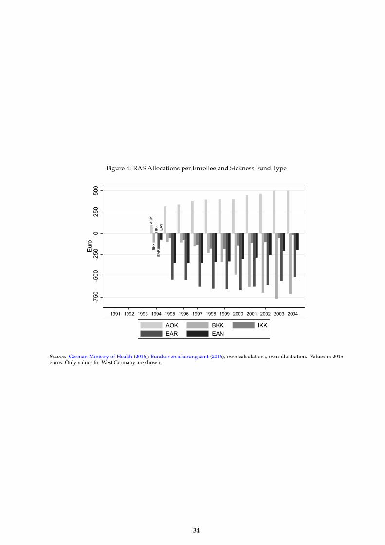
Figure 4: RAS Allocations per Enrollee and Sickness Fund Type

AO

KB

KK

IKK

EA

RE

AN

-500

050

025

0-2

50-7

50E

uro

1991 1992 1993 1994 1995 1996 1997 1998 1999 2000 2001 2002 2003 2004

AOK BKK IKKEAR EAN

Source: German Ministry of Health (2016); Bundesversicherungsamt (2016), own calculations, own illustration. Values in 2015euros. Only values for West Germany are shown.

34

Figure 5: Increase in Switching Probability after Introduction of Free Health Plan Choice

0.0

2.0

4.0

6.0

8.1

Sw

itchi

ng p

roba

bilit

y

1996 1998 2000 20021995 1997 1999 2001 2003

Switching HI Lower boundUpper bound

Note: Year dummies of column (2) in Table 4 are plotted. The reference point is the year before switching became a legalright, 1995.

Figure 6: Cumulative Switching Probability after Introduction of Free Health Plan Choice

0.1

.2.3

Cum

ulat

ive

switc

hing

pro

babi

lity

1996 1998 2000 20021995 1997 1999 2001 2003

Switching HI since '96 Lower boundUpper bound

Note: Year dummies of column (4) in Table 4 are plotted. The reference point is the year before switching became a legalright, 1995.

35

Figure 7: Change in Socio-Demographics across Sickness Fund Categories Pre and Post 1996

-.3 -.2 -.1 0 .1 .2

Married

Age

Female

Socio-demographicsPre-Post 1996 differences

AOK BKKIKK EAREAN

Source: SOEP Long v30. The figure is a nonparametric plot of equation (6).

Figure 8: Change in Health Status across Sickness Fund Categories Pre and Post 1996

-.15 -.1 -.05 0 .05 .1

SWH - Highest

SWH - High

SWH - Medium

SWH - Low

SWH - Lowest

Hospital visit

Disability

Health statusPre-Post 1996 differences

AOK BKKIKK EAREAN

Source: SOEP Long v30. The figure is a nonparametric plot of equation (6).

36

Table 1: Meaning and History of Sickness Fund Categories

German Name English Translation Abbr. History and Enrollment

Bundesknappschaft Federal Miners’ Guild BKN Miners and relatives. In 1995: 1.2M enrollees.4.8% female, age 42.4, gross wage e 3719, 59.3% blue collar, disabled: 3.7%

Innungskrankenkasse Guilds’ Sickness Fund IKK Craftsmen and relatives. In 1995: 2.9M enrollees.12.7% female, age 37.2, gross wage e 2692, 78.9% blue collar, disabled: 4.6%

Betriebskrankenkassen Company Sickness Fund BKK Employees and relatives. In 1995: 5.2M enrollees.23.9% female, age 39.5, gross wage e 3309, 49.1% blue collar, disabled: 5.8%

Ersatzkassen fur Arbeiter Alternative Funds for Blue Collar Workers EAR Blue collar workers prior to 1883. In 1995: 0.9M enrollees.17.7% female, age 38.0, gross wage e 2854, 86.4% blue collar, disabled: 7.3%

Ersatzkassen fur Arbeitnehmer Alternative Funds for White Collar Workers EAN White collar workers prior to 1883. In 1995: 17.5M enrollees.42.7% female, age 39.5, gross wage e 3370, 4.4% blue collar, disabled: 5.9%

Allgemeine Ortskrankenkassen General Town Sickness Funds AOK Blue collar workers who could not be assigned. In 1995: 22.3M enrollees.25.5% female, age 39.7, gross wage e 2610, 74.2% blue collar, disabled: 6.7%

Sources: German Federal Statistical Office (2017), Table A2

Table 2: Estimating the RAS Pass-Through Rate

Model 1(1)

Model 2(2)

Model 3(3)

Panel Ayit: Contribution rate in ppt.RAS/[enrolleet−1×1000] 0.558 -0.794*** -0.782***

(0.325) (0.121) (0.099)Mean dependent variable 13.451 13.451 13.451

Panel Byit: Annual employee share of premium (in 2015 euros)RAS/enrolleet−1 -0.291* -0.181** -0.211***

(0.121) (0.068) (0.039)Mean dependent variable 2,339 2,339 2,339

Panel Cyit: Reserves/enrolleeRAS/enrolleet−1 0.026 0.054 0.055*

(0.053) (0.027) (0.027)Mean dependent variable 71.986 71.986 71.986

Panel Dyit: Assets/enrolleeRAS/enrolleet−1 0.144** 0.136*** 0.128***

(0.053) (0.027) (0.027)Mean dependent variable 190.847 190.847 190.847

Panel Eyit: Administrative costs/enrolleeRAS/enrolleet−1 0.031 -0.001 0.002

(0.018) (0.017) (0.013)Mean dependent variable 119.048 119.048 119.048

Panel Fyit: Health care spending/enrolleeRAS/enrolleet−1 0.574*** 0.257 0.222

(0.047) (0.152) (0.122)Mean dependent variable 2,109 2,109 2,109

Panel Gyit: Premium revenues/enrolleeRAS/enrolleet−1 -0.557*** -0.769*** -0.752***

(0.061) (0.105) (0.093)Mean dependent variable 2,230 2,230 2,230

Year FE × × ×State FE × × ×Sickness fund category FE × ×Individual FE ×Age, gender, disability ×Other covariates ×Sources: SOEP Long v30; Wagner et al. (2007); Socio-Economic Panel (SOEP) (2015); Deutscher Bundestag(2004); Muller and Lange (2010); German Ministry of Health (2016); Bundesversicherungsamt (2016); Ger-man Federal Statistical Office (2016a). * p<0.1, ** p<0.05, *** p<0.01; standard errors in parentheses areclustered on the health plan type level. Each column in each panel represents one regression with N=50,501and the years 1991-2004 (except for Panel D where N=42,548 and the years include 1991-2002). SOEP pro-vided weights are used and monetary values are in 2015 euros. Descriptive Statistics are in Table A1.

38

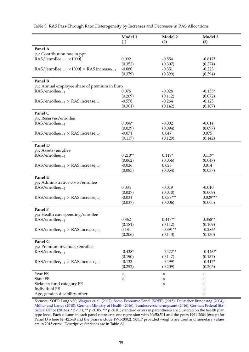
Table 3: RAS Pass-Through Rate: Heterogeneity by Increases and Decreases in RAS Allocations

Model 1(1)

Model 2(2)

Model 3(3)

Panel Ayit: Contribution rate in ppt.RAS/[enrolleet−1 ×1000] 0.092 -0.554 -0.617*

(0.352) (0.307) (0.274)RAS/[enrolleet−1 ×1000] × RAS increaset−1 -0.080 -0.351 -0.223

(0.379) (0.399) (0.394)

Panel Byit: Annual employee share of premium in EuroRAS/enrolleet−1 0.076 -0.028 -0.155*

(0.209) (0.112) (0.072)RAS/enrolleet−1 × RAS increaset−1 -0.558 -0.264 -0.125

(0.301) (0.142) (0.107)

Panel Cyit: Reserves/enrolleeRAS/enrolleet−1 0.084* -0.002 -0.014

(0.039) (0.094) (0.097)RAS/enrolleet−1 × RAS increaset−1 -0.071 0.047 0.075

(0.117) (0.129) (0.142)

Panel Dyit: Assets/enrolleeRAS/enrolleet−1 0.210** 0.119* 0.119*

(0.062) (0.056) (0.047)RAS/enrolleet−1 × RAS increaset−1 -0.026 0.023 0.014

(0.085) (0.054) (0.037)

Panel Eyit: Administrative costs/enrolleeRAS/enrolleet−1 0.034 -0.019 -0.010

(0.027) (0.010) (0.009)RAS/enrolleet−1 × RAS increaset−1 -0.031 0.038*** 0.029***

(0.037) (0.006) (0.005)

Panel Fyit: Health care spending/enrolleeRAS/enrolleet−1 0.362 0.447** 0.358**

(0.181) (0.112) (0.109)RAS/enrolleet−1 × RAS increaset−1 0.181 -0.391** -0.286*

(0.206) (0.143) (0.130)

Panel Gyit: Premium revenues/enrolleeRAS/enrolleet−1 -0.438* -0.422** -0.446**

(0.190) (0.147) (0.137)RAS/enrolleet−1 × RAS increaset−1 -0.133 -0.499* -0.417*

(0.252) (0.209) (0.205)

Year FE × × ×State FE × × ×Sickness fund category FE × ×Individual FE ×Age, gender, disability, other ×Sources: SOEP Long v30; Wagner et al. (2007); Socio-Economic Panel (SOEP) (2015); Deutscher Bundestag (2004);Muller and Lange (2010); German Ministry of Health (2016); Bundesversicherungsamt (2016); German Federal Sta-tistical Office (2016a). * p<0.1, ** p<0.05, *** p<0.01; standard errors in parentheses are clustered on the health plantype level. Each column in each panel represents one regression with N=50,501 and the years 1991-2004 (except forPanel D where N=42,548 and the years include 1991-2002). SOEP provided weights are used and monetary valuesare in 2015 euros. Descriptive Statistics are in Table A1.

39

Table 4: Who Switches?

Switched Health Plan Last Year Switched Health Plan Since 1996Demographics (1) (2) (3) (4)

Age 18 to 25 0.0278*** 0.0251*** 0.0012 0.0034(0.0069) (0.0072) (0.0084) (0.0090)

Age 26 to 35 0.0339*** 0.0287*** 0.0669*** 0.0601***(0.0048) (0.0048) (0.0065) (0.0065)

Age 46 to 55 -0.0205*** -0.0244*** -0.0415*** -0.0484***(0.0042) (0.0044) (0.0061) (0.0065)

Age 56 to 64 -0.0431*** -0.0493*** -0.0791*** -0.0897***(0.0043) (0.0048) (0.0071) (0.0078)

Female 0.0128*** 0.0021 0.0120** 0.0009(0.0039) (0.0044) (0.0051) (0.0058)

# persons < 16 in HH -0.0071*** -0.0123***(0.0019) (0.0027)

Owner -0.0051 0.0047(0.0036) (0.0051)

Education and Labor Market

White collar 0.0210*** 0.0251***(0.0042) (0.0057)

1st wage quartile 0.0007 -0.0026(0.0054) (0.0070)

3rd wage quartile 0.0070 0.0219***(0.0051) (0.0069)

4th wage quartile 0.0022 0.0085(0.0055) (0.0073)

Vocational degree 0.0180* 0.0466***(0.0093) (0.0121)

Higher education 0.0054 0.0226**(0.0070) (0.0095)

Health Status

Disability -0.0062 -0.0062 -0.0140 -0.0133(0.0059) (0.0060) (0.0101) (0.0103)

Hospital stay -0.0108* -0.0100 0.0043 0.0062(0.0063) (0.0063) (0.0104) (0.0104)

SWH - low -0.0032 -0.0044 0.0080 0.0059(0.0104) (0.0104) (0.0167) (0.0166)

SWH - medium 0.0044 0.0043 0.0102 0.0099(0.0097) (0.0097) (0.0152) (0.0152)

SWH - high 0.0060 0.0039 0.0098 0.0056(0.0097) (0.0097) (0.0153) (0.0152)

SWH - highest -0.0061 -0.0083 -0.0167 -0.0209(0.0099) (0.0099) (0.0156) (0.0155)

Mean dependent variable 0.0675 0.0675 0.1498 0.1498

R2 0.0219 0.0248 0.0713 0.0758

Sources: SOEP Long v30. Notes: Wagner et al. (2007); Socio-Economic Panel (SOEP) (2015); Mullerand Lange (2010); German Ministry of Health (2016); Bundesversicherungsamt (2016). * p<0.1, **p<0.05, *** p<0.01; standard errors in parentheses are clustered on the individual level. Each col-umn represents one regression. All columns use the years 1996-2004. n=34,038. SOEP providedweights are used. Middle vocational and higher vocational covariates not shown (small and n.s.).All regressions include state and year fixed effects. Descriptive Statistics are in Table A1.

40

Table 5: Who Paid Higher Premiums Pre and Post-RAS?

Contribution Rate RAS Allocation(1) (2)

Demographics

Age 18 to 25 -0.0674*** -0.0150(0.0161) (0.0103)

Age 18 to 25 × Post-RAS 0.0338*(0.0198)

Age 26 to 35 -0.0121 -0.0190***(0.0126) (0.0061)

Age 26 to 35 × Post-RAS -0.0277*(0.0147)

Age 46 to 55 -0.0286** 0.0412***(0.0140) (0.0068)

Age 46 to 55 × Post-RAS 0.0787***(0.0162)

Age 56 to 64 0.0500*** 0.0717***(0.0193) (0.0085)

Age 56 to 64 × Post-RAS 0.0455**(0.0219)

Female 0.0333*** -0.0264***(0.0116) (0.0057)

Female × Post-RAS -0.0271**(0.0135)

# persons < 16 in HH 0.0174*** 0.0231***(0.0055) (0.0027)

# persons < 16 in HH × Post-RAS 0.0008(0.0065)

Owner 0.0488*** -0.0145***(0.0095) (0.0049)

Owner × Post-RAS -0.0569***(0.0113)

Education and Labor Market

White collar -0.1012*** -0.2092***(0.0115) (0.0060)

White collar × Post-RAS 0.1343***(0.0135)

1st wage quartile 0.0998*** 0.0364***(0.0128) (0.0074)

1st wage quartile × Post-RAS -0.0426***(0.0152)

3rd wage quartile -0.0898*** -0.0673***(0.0137) (0.0068)

3rd wage quartile × Post-RAS -0.0036(0.0160)

4th wage quartile -0.1898*** -0.1257***(0.0156) (0.0073)

4th wage quartile × Post-RAS 0.0453**(0.0180)

Higher education 0.0366* -0.1110***(0.0203) (0.0091)

Higher education × Post-RAS -0.0302(0.0234)

Health Status

Disability -0.0240 0.0102(0.0207) (0.0103)

Disability × Post-RAS 0.0427*(0.0238)

Hospital stay -0.0168 0.0134(0.0174) (0.0099)

Hospital stay × Post-RAS 0.0239(0.0208)

Sources: SOEP Long v30. Notes: Wagner et al. (2007); Socio-Economic Panel (SOEP) (2015); Muller and Lange (2010);German Ministry of Health (2016); Bundesversicherungsamt (2016). * p<0.1, ** p<0.05, *** p<0.01; standard errors inparentheses are clustered on the individual level. Each column in each panel represents one regression. Column (1) usethe years 1984-2004 (N=68,641) and column (2) uses the years 1994-2004 (N=40,387). SOEP provided weights are used.All regressions include year fixed effects. The following insignificant covariates in levels and interaction are not showndue to space contrains: all SWH measures, middle vocational, vocational and higher vocational. Descriptive Statistics arein Table A1.

Table 6: Relationship between Contribution Rates and Premiums: RAS Allocations as IV

Income Quartiles Mean Q1 Q2 Q3 Q4(1) (2) (3) (4) (5)

Panel ADependent variable: Annual premium in euro (prices as of 2015)

Contribution ratet 222.317*** 128.055*** 146.154*** 200.596*** 250.915***(18.107) (11.311) (3.162) (5.630) (12.713)

R2 0.315 0.219 0.467 0.492 0.678N 50,501 10,727 11,957 12,959 14,858Mean dependent variable 2,339 1,468 1,942 2,375 3,093

Panel BDependent variable: Annual premium in euro (prices as of 2015)Variable of interest: RAS/enrolleet−1 as instrument for contribution rate

Contribution ratet 268.111*** 104.912*** 162.608*** 206.789*** 254.152***(11.244) (15.271) (9.073) (11.129) (13.304)

F-statistic (first stage) 59.595*** 223.618*** 138.050*** 64.728*** 22.230***R2 0.314 0.218 0.467 0.492 0.678N 50,501 10,727 11,957 12,959 14,858

Year FE × × × × ×State FE × × × × ×Sickness fund category FE × × × × ×Individual FE × × × × ×Age, gender, disability × × × × ×Other covariates × × × × ×Sources: SOEP Long v30; Wagner et al. (2007); Socio-Economic Panel (SOEP) (2015); Muller and Lange(2010); German Ministry of Health (2016); Bundesversicherungsamt (2016). * p<0.1, ** p<0.05, *** p<0.01;Standard errors in parentheses are clustered on the health plan type level. All models use the years 1994-2004. SOEP provided weights are used. Each column in each panel represents one regression model. PanelA contains OLS regressions and Panel B IV-2SLS regressions where the contribution rate is instrumentedwith RAS allocations per year and enrollee. Descriptive Statistics are in Table A1.

42

Appendix

Figure A1: Consumer Savings after Health Plan Switching

020

4060

8010

0E

uro

1996 1998 2000 20021995 1997 1999 2001 2003

Savings from switch Lower boundUpper bound

Note: Year dummies of a regression of Savings per switch on year dummies and all covariates are plotted. The referencepoint is the last year before switching became a legal right, 1995.

43

Table A1: Descriptive Statistics

Mean SD Min Max N

Health Insurance

Contribution rate 13.058 (0.959) 10.130 14.650 75,646Contribution 2,200 (636) 752 3,618 75,646RAS/enrollee -66.757 (369.195) -766.748 1,426 50,501Reserves/enrollee 71.986 (114.443) -212.054 935.383 50,501Assets/enrollee 190.847 (85.461) 68.333 1,118 42,548Administrative costs/enrollee 119.048 (29.057) 28.073 166.451 50,501Health care spending/enrollee 2,109 (258) 1,575 3,674 50,501Premium revenues/enrollee 2,230 (265) 1,602 2,709 50,501Switched HI last year 0.031 (0.174) 0.000 1.000 75,646Switched HI since ’96 0.069 (0.254) 0.000 1.000 75,646# Changes since ’96 0.228 (0.610) 0.000 6.000 75,646Savings per switch 1.569 (19.690) -312.737 452.228 75,646Cond. savings per switch 50.401 (99.996) -312.737 452.228 2,241

Demographics

Female 0.299 (0.458) 0.000 1.000 75,646Age 39.397 (11.141) 18.000 64.000 75,64618-25 years 0.116 (0.320) 0.000 1.000 75,64626-35 years 0.299 (0.458) 0.000 1.000 75,64636-45 years 0.263 (0.440) 0.000 1.000 75,64646-55 years 0.227 (0.419) 0.000 1.000 75,64656-64 years 0.095 (0.294) 0.000 1.000 75,646Married 0.629 (0.483) 0.000 1.000 75,646# persons in HH 2.891 (1.325) 1.000 17.000 75,646# persons < 16 in HH 0.551 (0.890) 0.000 9.000 75,646Owner 0.436 (0.496) 0.000 1.000 75,646

Education and Labor Market

Gross wage 3,007 (1,312) 940 58,450 75,6461st wage quantile 0.225 (0.417) 0.000 1.000 75,6462nd wage quantile 0.236 (0.425) 0.000 1.000 75,6463rd wage quantile 0.255 (0.436) 0.000 1.000 75,6464th wage quantile 0.284 (0.451) 0.000 1.000 75,646Net wage 1,941 (796) 60.000 18,514 75,646White collar 0.532 (0.499) 0.000 1.000 75,646Blue collar 0.468 (0.499) 0.000 1.000 75,646Inadequate + elementary edu. 0.161 (0.367) 0.000 1.000 75,646Middle vocational 0.583 (0.493) 0.000 1.000 75,646Vocational degree 0.053 (0.224) 0.000 1.000 75,646Higher vocational degree 0.096 (0.295) 0.000 1.000 75,646Higher education 0.107 (0.309) 0.000 1.000 75,646

Health Status

Disability 0.062 (0.241) 0.000 1.000 75,646Hospital stay 0.080 (0.272) 0.000 1.000 68,641SWH - lowest (0-2/10) 0.030 (0.171) 0.000 1.000 75,646SWH - low (3-4/10) 0.082 (0.275) 0.000 1.000 75,646SWH - medium (5-6/10) 0.218 (0.413) 0.000 1.000 75,646SWH - high (7-8/10) 0.432 (0.495) 0.000 1.000 75,646SWH - highest (9-10/10) 0.238 (0.426) 0.000 1.000 75,646

Sources: SOEP Long v30; Wagner et al. (2007); Socio-Economic Panel (SOEP) (2015); Muller andLange (2010); German Ministry of Health (2016); Bundesversicherungsamt (2016). SWH–satisfactionswith health. SOEP provided weights are used.

44

Table A2: Descriptive Statistics by Type of Sickness Fund

Mean AOK BKK IKK BKN EAR EAN

Health Insurance

Contribution 2,200 2,059 2,242 2,055 2,549 2,098 2,373(636) (578) (619) (561) (547) (621) (675)

Contribution rate 13.058 13.428 12.266 12.992 13.125 12.523 13.121(0.959) (0.724) (1.083) (0.913) (0.392) (1.074) (0.846)

RAS/enrollee -66.757 307.424 -439.258 -82.047 1,383 -445.821 -224.528(369.195) (182.305) (282.657) (65.653) (51.847) (257.064) (134.315)

Reserves/enrollee 71.986 55.171 39.594 76.969 669.831 60.226 102.070(114.443) (85.484) (135.541) (136.874) (329.638) (134.367) (84.786)

Assets/enrollee 190.847 208.224 164.017 297.613 1,036 180.475 158.349(85.461) (23.562) (68.208) (112.884) (79.566) (109.466) (59.393)

Administrative costs/enrollee 119.048 128.098 72.391 123.256 156.672 100.346 137.566(29.057) (14.944) (25.687) (7.904) (7.802) (5.234) (9.221)

Health care spending/enrollee 2,109 2,352 1,980 1,761 3,538 1,740 2,013(258) (145) (96) (101) (113) (97) (151)

Premium revenues/enrollee 2,230 2,065 2,436 1,980 2,194 2,244 2,334(265) (95) (248) (173) (52) (333) (261)

Switched HI last year 0.031 0.009 0.111 0.021 0.042 0.041 0.015(0.174) (0.092) (0.314) (0.144) (0.201) (0.198) (0.121)

Switched HI since 1996 0.069 0.024 0.229 0.056 0.067 0.073 0.038(0.254) (0.152) (0.420) (0.230) (0.250) (0.261) (0.190)

# Changes since 1996 0.228 0.163 0.437 0.229 0.116 0.252 0.189(0.610) (0.498) (0.832) (0.615) (0.437) (0.659) (0.553)

Savings by switch 1.569 -0.103 9.049 0.152 8.566 1.209 -0.287(19.690) (3.628) (42.667) (10.909) (54.667) (16.253) (7.180)

Cond. savings per switch 50.401 -11.991 81.448 7.149 203.364 29.559 -19.205(99.996) (37.421) (102.443) (74.895) (186.790) (75.403) (55.644)

Demographics

Female 0.299 0.255 0.239 0.127 0.048 0.177 0.427(0.458) (0.436) (0.426) (0.333) (0.215) (0.381) (0.495)

Age 39.397 39.718 39.466 37.235 42.429 38.015 39.508(11.141) (11.493) (10.528) (11.111) (9.983) (10.776) (11.043)

18-25 years 0.116 0.129 0.091 0.159 0.036 0.137 0.104(0.320) (0.335) (0.288) (0.365) (0.186) (0.344) (0.305)

26-35 years 0.299 0.273 0.311 0.351 0.264 0.324 0.311(0.458) (0.446) (0.463) (0.477) (0.442) (0.468) (0.463)

36-45 years 0.263 0.255 0.285 0.227 0.230 0.262 0.267(0.440) (0.436) (0.452) (0.419) (0.422) (0.440) (0.442)

46-55 years 0.227 0.236 0.236 0.194 0.406 0.205 0.220(0.419) (0.425) (0.424) (0.395) (0.492) (0.404) (0.414)

56-64 years 0.095 0.107 0.077 0.069 0.065 0.072 0.099(0.294) (0.309) (0.267) (0.254) (0.246) (0.259) (0.299)

Married 0.629 0.650 0.656 0.626 0.789 0.635 0.590(0.483) (0.477) (0.475) (0.484) (0.409) (0.481) (0.492)

# persons in HH 2.891 3.060 2.862 2.987 3.163 2.980 2.684(1.325) (1.384) (1.265) (1.358) (1.550) (1.329) (1.245)

# persons < 16 in HH 0.551 0.606 0.565 0.602 0.658 0.624 0.464(0.890) (0.924) (0.886) (0.906) (0.959) (1.008) (0.827)

Owner 0.436 0.410 0.436 0.395 0.421 0.464 0.470(0.496) (0.492) (0.496) (0.489) (0.495) (0.499) (0.499)

Education and Labor Market

Gross wage 3,007 2,610 3,309 2,692 3,719 2,854 3,370(1,312) (892) (1,373) (903) (1,689) (936) (1,597)

1st wage quantile 0.225 0.308 0.130 0.256 0.065 0.218 0.177(0.417) (0.462) (0.336) (0.436) (0.248) (0.413) (0.382)

2nd wage quantile 0.236 0.290 0.200 0.286 0.131 0.211 0.186Continued on next page...

45

... table A2 continuedMean AOK BKK IKK BKN EAR EAN(0.425) (0.454) (0.400) (0.452) (0.338) (0.408) (0.390)

3rd wage quantile 0.255 0.252 0.292 0.293 0.334 0.315 0.226(0.436) (0.434) (0.455) (0.455) (0.473) (0.465) (0.418)

4th wage quantile 0.284 0.150 0.379 0.165 0.469 0.256 0.410(0.451) (0.357) (0.485) (0.371) (0.500) (0.436) (0.492)

Net wage 1,941 1,726 2,125 1,782 2,423 1,867 2,121(796) (584) (850) (590) (883) (597) (943)

White collar 0.532 0.259 0.509 0.211 0.407 0.137 0.956(0.499) (0.438) (0.500) (0.408) (0.492) (0.343) (0.204)

Blue collar 0.468 0.742 0.491 0.789 0.593 0.864 0.044(0.499) (0.438) (0.500) (0.408) (0.492) (0.343) (0.204)

Inadequate + elementary edu. 0.161 0.256 0.156 0.139 0.056 0.146 0.060(0.367) (0.436) (0.363) (0.346) (0.230) (0.354) (0.237)

Middle vocational 0.583 0.609 0.578 0.718 0.687 0.669 0.522(0.493) (0.488) (0.494) (0.450) (0.465) (0.471) (0.500)

Vocational degree 0.053 0.040 0.067 0.030 0.034 0.031 0.068(0.224) (0.196) (0.250) (0.170) (0.181) (0.175) (0.251)

Higher vocational degree 0.096 0.062 0.083 0.089 0.115 0.130 0.140(0.295) (0.242) (0.276) (0.285) (0.320) (0.336) (0.347)

Higher education 0.107 0.032 0.116 0.024 0.108 0.024 0.210(0.309) (0.177) (0.320) (0.153) (0.312) (0.152) (0.407)

Health Status

Disability 0.062 0.067 0.058 0.046 0.037 0.073 0.059(0.241) (0.250) (0.233) (0.211) (0.190) (0.260) (0.236)

Hospital stay 0.080 0.086 0.077 0.075 0.103 0.083 0.075(0.272) (0.280) (0.267) (0.263) (0.304) (0.277) (0.264)

SWH - lowest 0.030 0.035 0.026 0.028 0.013 0.036 0.027(0.171) (0.183) (0.160) (0.165) (0.112) (0.187) (0.161)

SWH - low 0.082 0.087 0.087 0.073 0.088 0.083 0.076(0.275) (0.282) (0.281) (0.260) (0.284) (0.276) (0.265)

SWH - medium 0.218 0.239 0.219 0.220 0.179 0.209 0.193(0.413) (0.426) (0.414) (0.414) (0.384) (0.407) (0.395)

SWH - high 0.432 0.402 0.437 0.446 0.448 0.449 0.458(0.495) (0.490) (0.496) (0.497) (0.498) (0.498) (0.498)

SWH - highest 0.238 0.237 0.231 0.234 0.273 0.222 0.246(0.426) (0.425) (0.422) (0.423) (0.446) (0.416) (0.431)

Observations 75,646 33,658 14,181 4,617 221 2,023 20,946

Sources: SOEP Long v30; Wagner et al. (2007); Socio-Economic Panel (SOEP) (2015); Muller and Lange (2010);German Ministry of Health (2016); Bundesversicherungsamt (2016). SWH – satisfactions with health; SAH –self-assessed health. SOEP provided weights are used.

46

Table A3: Differences in Socio-Demographics by Sickness Fund Type

AOK BKK IKK BKN EAR EAN

18-25 years -0.115*** 0.075*** 0.042*** 0.001 0.019*** -0.022(0.019) (0.015) (0.009) (0.001) (0.007) (0.015)

26-35 years -0.090*** 0.070*** 0.031*** 0.001 0.017*** -0.028**(0.016) (0.013) (0.008) (0.001) (0.006) (0.013)

36-45 years -0.056*** 0.048*** 0.010 -0.001 0.010* -0.011(0.015) (0.013) (0.008) (0.001) (0.005) (0.013)

46-55 years -0.039*** 0.037*** 0.009 0.003** 0.006 -0.014(0.012) (0.010) (0.006) (0.001) (0.004) (0.010)

Female -0.017 -0.007 -0.042*** -0.002*** 0.008* 0.060***(0.012) (0.010) (0.005) (0.001) (0.004) (0.011)

Married 0.003 0.020** -0.001 0.001 -0.006 -0.017*(0.011) (0.009) (0.005) (0.001) (0.004) (0.009)

# persons < 16 in HH 0.018*** -0.014*** -0.002 -0.000 -0.000 -0.001(0.005) (0.005) (0.003) (0.000) (0.003) (0.004)

Owner -0.010 -0.008 -0.001 -0.001 0.008** 0.012(0.010) (0.009) (0.006) (0.001) (0.004) (0.008)

Disability 0.011 -0.007 -0.013 -0.002* 0.009 0.002(0.019) (0.016) (0.012) (0.001) (0.007) (0.016)

SWH - lowest -0.004 -0.013 -0.003 -0.000 0.003 0.017(0.016) (0.013) (0.007) (0.001) (0.007) (0.013)

SWH - low -0.005 0.008 -0.005 0.001 -0.000 0.001(0.010) (0.010) (0.005) (0.001) (0.003) (0.008)

SWH - high -0.013* -0.006 0.002 0.000 0.004 0.013**(0.007) (0.006) (0.004) (0.001) (0.003) (0.006)

SWH - highest 0.002 -0.008 -0.005 0.001 0.001 0.009(0.010) (0.008) (0.005) (0.001) (0.003) (0.008)

1st wage quantile 0.056*** -0.055*** 0.009* 0.000 0.006 -0.017**(0.009) (0.007) (0.005) (0.000) (0.004) (0.007)

3rd wage quantile -0.071*** 0.057*** -0.006 0.001* 0.013*** 0.006(0.009) (0.008) (0.005) (0.001) (0.004) (0.007)

4th wage quantile -0.142*** 0.104*** -0.024*** 0.002** 0.021*** 0.039***(0.012) (0.011) (0.006) (0.001) (0.005) (0.011)

White collar -0.342*** -0.036*** -0.069*** -0.001 -0.071*** 0.519***(0.012) (0.010) (0.006) (0.001) (0.005) (0.010)

Middle vocational -0.084*** -0.031** 0.041*** 0.002** 0.023*** 0.050***(0.014) (0.012) (0.008) (0.001) (0.005) (0.009)

Vocational degree -0.085*** -0.004 0.006 -0.001 0.016*** 0.068***(0.021) (0.021) (0.010) (0.001) (0.006) (0.020)

Higher vocational degree -0.107*** -0.073*** 0.047*** 0.001 0.050*** 0.082***(0.021) (0.018) (0.011) (0.002) (0.008) (0.018)

Higher education -0.133*** -0.064*** 0.018** -0.000 0.017*** 0.163***(0.019) (0.019) (0.008) (0.002) (0.005) (0.019)

Constant 0.726*** 0.092*** 0.044*** -0.004*** 0.043*** 0.099***(0.034) (0.026) (0.016) (0.002) (0.013) (0.028)

R2 0.240 0.057 0.053 0.013 0.036 0.405Mean dependent variable 0.386 0.181 0.064 0.003 0.034 0.333

Sources: SOEP Long v30. * p<0.1, ** p<0.05, *** p<0.01; standard errors in parentheses are clusteredat the individual level. Each column in each panel represents one regression with N=75,646. Allregressions use year and state fixed effects. SOEP provided weights are used.

47

Table A4: Estimating the RAS Pass-Through Rate: Robustness with T=0

Model 1(1)

Model 2(2)

Model 3(3)

Panel Ayit: Contribution rate in ppt.RAS/[enrolleet ×1000] 0.608* -0.773*** -0.773***

(0.300) (0.187) (0.167)

Panel Byit: Annual employee share of premium in Euro)RAS/enrolleet -0.266* -0.174* -0.209**

(0.118) (0.081) (0.054)

Panel Cyit: Reserves/enrolleeRAS/enrolleet 0.021 0.059* 0.061*

(0.047) (0.025) (0.027)

Panel Dyit: Assets/enrolleeRAS/enrolleet 0.120** 0.120*** 0.110***

(0.046) (0.025) (0.025)

Panel Eyit: Administrative costs/enrolleeRAS/enrolleet 0.031 -0.004 0.000

(0.017) (0.018) (0.014)

Panel Fyit: Health care spending/enrolleeRAS/enrolleet 0.543*** 0.297 0.259*

(0.040) (0.149) (0.128)

Panel Gyit: Premium revenues/enrolleeRAS/enrolleet -0.510*** -0.783*** -0.800***

(0.054) (0.146) (0.123)

Year FE × × ×State FE × × ×Sickness fund category FE × ×Individual FE ×Age, gender, disability ×Other covariates ×Sources: SOEP Long v30; Wagner et al. (2007); Socio-Economic Panel (SOEP) (2015); Deutscher Bun-destag (2004); Muller and Lange (2010); German Ministry of Health (2016); Bundesversicherungsamt(2016); German Federal Statistical Office (2016a). * p<0.1, ** p<0.05, *** p<0.01; standard errors inparentheses are clustered on the health plan type level. Each column in each panel represents oneregression with N=50,501 and the years 1991-2004 (except for Panel D where N=42,548 and the yearsinclude 1991-2002). SOEP provided weights are used and monetary values are in 2015 euros. De-scriptive Statistics are in Table A1.

48