Introducing Environmental Taxes in Russia: Relevance of Tax-Interaction Effects

Anton Orlov and Harald Grethe

Abstract The theoretical literature on the double dividend concept is mainly focused in pre-existing distortionary taxes in the labour and capital market; however, the relevance of interactions with other taxes and tariffs is often neglected. Using an analytical model and a numerical general equilibrium model, we analyze the incidence of carbon taxes as well as tax interactions in Russia. The main findings are the following: substituting carbon taxes for labour taxes can lead to increases in revenues from export taxes, import tariffs, value added taxes, and some excise taxes because of the expansion of tax bases. Increases in revenues from taxes and tariffs decrease the cost of environmental tax reform. On the other hand, revenues from taxes on labour and capital income, mineral resource extraction taxes, excise taxes on petroleum products, and social security contribution decrease.

JEL classification code: Q50, H20, C30, C68

Key words: carbon taxes; Russia; tax-interaction effect.

Anton Orlov, Department of Agriculture and Food Policy (420a), University of Hohenheim, Schloß, Osthof-Süd. 70599 Stuttgart. Email: orlov@uni-hohenheim.de Tel: 0711 459-22522 Fax: 0711 459-23752

Harald Grethe, Department of Agriculture and Food Policy (420a), University of Hohenheim, Schloß, Osthof-Süd. 70599 Stuttgart. Email: grethe@uni-hohenheim.de Tel: 0711 459-22631 Fax: 0711 459-23752

1

Contents

1 Introduction ........................................................................................................................... 3

2 Tax System in Russia ............................................................................................................ 4

3 Theoretical Background ..................................................................................................... 11

4 Numerical Model ................................................................................................................. 17 4.1 Model and Database ....................................................................................................... 17 4.2 Experiments and Model Closures .................................................................................. 18

5 Results .................................................................................................................................. 19

6 Conclusions .......................................................................................................................... 26

References ............................................................................................................................... 28

Appendices .............................................................................................................................. 30 Appendix A: Derivation of Equation (3.21)......................................................................... 30 Appendix B: Numerical Model ............................................................................................ 32 Appendix C: Elasticities in the Model ................................................................................. 35

2

1 Introduction

Russia is not only one of the world’s major sources of carbon energy – coal, oil and gas – but

is also one the most intensive users of energy. Large energy saving potential can be realized

through technological modernization. Introducing carbon taxes would, potentially, address

concerns on several fronts simultaneously. In the short to medium term, they would reduce

the emission of CO2 and other emissions which are stemming from the use of energy

commodities. In the longer term, the increased costs of primary energy products should both

accelerate the rate of technological replacement and induce technological progress (Ruttan,

1997; Newell et al., 1999; Popp, 2002). Furthermore, according to the environmental taxation

literature, an introduction of environmental taxes is often related to the concept of double

dividend, where substituting environmental taxes for other distortionary taxes not only

benefits the environment, but also reduces efficiency costs of the tax system (Goulder, 1994).

The theoretical literature on environmental taxation is mainly focused on pre-existing

distortionary taxes in the labour and capital market (Goulder et al. 1997; de Mooij and

Bovenberg, 1998), whereas interactions with other taxes and tariffs such as imports tariffs,

export taxes, valued added taxes, excise taxes, and mineral resource extraction taxes are often

neglected. Introducing environmental taxes, however, can indirectly affect the efficiency of

the tax system through changes in the tax bases. As a result, carbon taxes can either alleviate

or exacerbate pre-existing distortions. Moreover, taxes other than labour and capital taxes can

be a large source of government revenues. For instance, revenues from import tariffs and

export taxes, especially export taxes on crude oil, petroleum products, and natural gas,

amount to approximately 21% of total government revenues in Russia (FSSS, 2010;

Roskazna, 2010).

The objectives of this analysis are the following: (1) to verify the hypothesis of a double

dividend of carbon taxes in Russia, (2) to analyse the incidence of carbon taxes, (3) to

investigate interactions of carbon taxes with other taxes and tariffs. This analysis is based on

an analytical model developed by Parry (2001) as well as a computable comparative static

general equilibrium model – an energy/environment adaptation of the STAGE model

(McDonald, 2007). To our knowledge this is the first such study for Russia. Moreover, this is

the first paper which explicitly treats the interaction between environmental and other taxes

by using a computable general equilibrium model. The paper is organised as follows. The

next section gives a brief overview on the Russian tax system, especially tax regimes applied

with respect to production, consumption and trade of energy commodities. Section three

3

provides a theoretical background of welfare effects resulting from an introduction of

environmental taxes. Section four gives a short description of the numerical model, database,

and experiment – an informal description of the model can be found in the appendix B. The

results of simulations are presented in section five. The final section summarises the main

results and discussions. The main findings are the following: substituting carbon taxes for

labour taxes can lead to increases in revenues from export and import taxes, value added

taxes, and some excise taxes because of expanding tax bases. Increases in revenues from taxes

decrease the cost of environmental tax reform. On the other hand, revenues from taxes on

labour and capital income, mineral resource extraction taxes, excise taxes on petroleum

products, and social security contribution decrease.

2 Tax System in Russia

Overview of the Russian Tax System. The Russian economy as well as other economies is

distorted by different taxes. In this section, we give a short overview of the Russian tax

system, especially the tax regime which is applied to production, consumption and trade of

energy commodities. Data on the tax system are taken from different legislative documents1,

which are summarized in Table 2.1. The documents were reviewed at March 2012.

Table 2.1 Legislative documents of the Russian tax system. Taxes and Tariffs Corresponding Legislative Documents

Value added tax, excise tax, corporate income tax, personal income tax, mineral resource extraction tax, and others

Russian Tax Code (second part) No.117-FZ from 5.Aug. 2000 (further Russian Tax Code)

Export taxes on crude oil and oil products Government Decree No.695 from 16.Nov 2006

Export taxes on other commodities Government Decree from 6. Feb. 2012 No. 88

Import tariffs Enactment No. 850 from 18. Nov. 2011

Calculation of export taxes on crude oil Law of Trade Tariffs No.5003-1 from 21.May 1993

Calculation of export taxes on oil products Government Decree No.1155 from 27.Dec. 2010

Fig. 2.1 illustrates the structure of government revenues in Russia in 2010. The largest source

of government revenues is trade taxes such as import and export taxes with a share of 20.8%

in total government revenues, following by value added taxes (16.1%), social security

contributions (16%), personal income taxes (11.6%), corporate income taxes (11.5%), and

mineral resource extraction taxes (9.8%). The magnitude of tax revenues depends on tax bases

and tax rates.

1 All documents are available (in Russian) at http://www.consultant.ru/.

4

Fig. 2.1 Structure of government revenues in 2010 (%).

20.8

16.1

16.0

11.6

11.5

9.8

5.8

4.1

3.0

1.3

0 5 10 15 20 25

Trade taxes

Value added taxes

Social secur. contr.

Personal income taxes

Corporate profit taxes

Mineral res. extr. taxes

Others payments

Property taxes

Excise taxes

Unified income taxes

share in %

Unified income taxes are taxes imposed according to the simplified tax system in Russia; Others payments are payments for the use of public property, free payments and others; Mineral res.extr.taxes states for mineral resource extraction taxes; Social secur.contr. states social security contributions; Source: FSSS (2010)

Trade taxes. In April 2010 the Customs Code of the Customs Union (further Customs Code)

came into force. The Customs Code is a legislative document, which regulates trade within

the Customs Union as well as trade with non-members of the Customs Union. The Customs

Union consists of the Republic of Belarus, the Republic of Kazakhstan and the Russian

Federation, and this allows for free trade between the members of the Union, whereas import

tariffs are imposed on Union’s imports. According to the Enactment No. 850 from 18.Nov.

2011, there are high import tariffs on some food products, textile products, machineries,

electronic equipment, and transports. For example in 2012, the import tariff rate on beef and

pork was at 15%, and on sheep meat and poultry it was at 25%. Import tariffs on textile

products, machineries, electronic equipment, and transports differ from product to product,

where tariff rates were between 5% and 30%. Import tariff rates on energy commodities

excluding electricity were at 5% in 2012.

High export taxes are imposed on commodities such as seeds, animal hide, timber, scrap

metals, and energy resources. For example according to Government Decree No.88 from

6.Feb. 2012, the rates of export taxes on seeds in 2012 were between 10% and 20%, 500 €/ton

for raw animal hides, between 10% and 25%, or 100 Euro/m3 for timber, and between 6.5%

5

and 50% for scrap metals. Revenues from trade taxes consist mainly of export taxes on energy

resources such as crude oil, oil products, and natural gas. For instance, the revenue share of

export taxes on crude oil was at 52% in the total revenues from trade taxes in 2010, for

petroleum products it was at 19% and for gas it was at 6% (Roskazna, 2012). There are no

export taxes on electricity and coal; however, an export tax on coke with a tax rate of 6.5%

was introduced in 2007. Export taxes on crude oil and oil products are specific. The rate of

export tax on crude oil is recalculated by the Russian Government each month in accordance

with changes in the price of Urals2 oil (Law of Trade Tariffs No.5003-1 from 21.May 1993).

The tax rate is calculated according to the formula, which is shown in Table 2.2.

Table 2.2 Formula for calculation of export taxes on crude oil.

Tax Regimes Formula

if PWoil < 109.5 $/ton then TEoil = 0%

if 109.5 $/ton < PWoil < 146 $/ton then TEoil = 0.35*(PWoil – 109.5 $/ton)

if 146 $/ton < PWoil< 182.5 $/ton then TEoil = 12.77 $/ton + 0.45*(PWoil – 146 $/ton)

if PWoil > 182.5 $/ton then TEoil = 29.2 $/ton + 0.65*(PWoil –182.5 $/ton)

where PWoil is the world price of Urals oil and TEoil is the rate of export tax on crude oil.

Source: Law of Trade Tariffs from 21.May 1993 No.5003-1

The formula for calculation of the export tax rate on crude oil includes four regimes,

depending on the price of Urals oil. For instance, the export price of Urals oil was at 774 $/ton

since 1.Jan. until 1. May 2011 (Ministry of Economics, 2011). Since the export price (PWoil)

was higher than 182.5$/ton, the specific export tax rate on crude oil (TEoil) is calculated as

follows:

29.2 $/ton + 0.65*(774 $/ton – 182.5 $/ton) = 413 $/ton (2.1)

Therefore, the rate of export tax on crude oil was at approximately 413 $/ton from January to

May in 2011, which amounts to approximately 53% of the export price of Urals oil. Rates of

export taxes on oil products depend on the export tax rate on crude oil. According to the

Government Decree from 27.Dec. 2010 No.1155, the rates of export taxes on oil products are

calculated as follows:

TEpetl = Kpetl* TEoil, (2.2)

where TEpetl are specific tax rates on oil products in $/ton, Kpetl are multiplier coefficients, and

TEoil is the specific export tax rate on crude oil in $/ton. From 2003 to 2010 the multiplier

coefficient was at 0.9 for all oil products. Since 2010 coefficients differ among oil products

2 Urals is an oil brand, whose prices are used to calculate export taxes on crude oil.

6

(Government Decree No.1155 from 27.Dec. 2010). Until 2015 the multiplier coefficients

should equal 0.66 for most oil products. The calculated rates of export taxes on crude oil and

oil products can be found in Government Decree No.695 from 16.Nov 2006.

The export tax rate on natural gas is at 30%, while the export tax rate on liquefied petroleum

gas (LPG) is specific and this is calculated according to the formula in Table 2.3. For

example, if the price of LPG is higher than 740 $/ton, then the specific tax rate on LPG equals

135 $/ton plus the difference between the observed average price and 740 $/ton, multiplied by

a coefficient is 0.7.

Table 2.3 Formula for calculation of export taxes on LPG.

Tax Regimes Formula

if PWgas < 490 $/ton then TELPG = K1*490

if 490 $/ton <PWgas < 640 $/ton then TELPG = K2*(PWgas – 490)

if 640 $/ton <PWgas < 740 $/ton then TELPG = 75 + K3*(PWgas – 640)

if PWgas > 740 $/ton then TELPG = 135 + K4*(PWgas – 740)

where PWgas is the average price of LPG observed on the border of Poland, TELPG is the specific rate of export tax on LPG, K1 = 0, K2 = 0.5, K3 = 0.6, K4 = 0.7.

Source: Government Decree No.1155 from 27.Dec.2010

Domestic Taxes. As shown in Table 2.4, the rate of corporate income tax was at 20%, the rate

of value added tax was at 18%, the flat tax rate on labour earnings was at 13%, and the rate of

social security contributions was at 34% in 2012. In February 2012, the rate of mineral tax on

extraction of crude oil was at approximately 411.2 $/ton, condensate gas (18.5 $/ton), and

natural gas (8 $/1000m3). The rate of excise tax on petrol (Euro-5) was at approximately 227

$/ton and for diesel (Euro-5) it was at approximately 119 $/ton in 2012.

7

Table 2.4 Tax system of the Russian Federation. Name of Taxes Tax Rates

Federal Taxes3: Corporate Income Tax

According to the Federal Law No.223-FZ from 26.Nov. 2008, the rate of corporate income tax was reduced from 24% to 20% in 2008.

Value Added Tax

According to the Federal Law No.117-FZ from 7.Jul. 2003, the rate of value added tax was reduced from 20% to 18% in 2003. Moreover, a tax rate of 10% is applied on some products such as food products, children’s clothing, books, education, and medical services. The tax rate on exported commodities equals 0%.

Personal Income Tax

The flat tax rate on labour income was at 13%, the tax rate on dividends was at 35%, tax rates on other personal income were at 9% or 30% in 2012.

Social Security Contributions

According to the Federal Law No. 212-FZ from 24.Jul. 2009, the unified social tax with a rate of 26% was replaced by social security contributions (SSC) with a rate of 34%. SSC are distributed between different funds: pension fund (26%), social insurance fund (2.9%), obligatory health insurance (5.1%).

Mineral Resource Extraction Tax

Mineral resources extraction taxes, inter alia, are imposed on condensate and natural gas, coal, and crude oil with different specific tax rates. For example, in February 2012 the rate of mineral tax on the extraction of crude oil was at approximately 411.2 $/ton, condensate gas (18.5 $/ton), and natural gas (8 $/1000m3). For more details see text below.

Excise Tax

Excise taxes are imposed on commodities such as alcohol, cigarettes, cars, and petroleum products with different specific tax rates. Rates of excise taxes on petroleum products differ among products according to their environmental impact. For example in 2012, the rate of excise tax on petrol (Euro-5) was at approximately 227 $/ton and for diesel (Euro-5) it was at approximately 119 $/ton. For more detail see text below.

Other taxes In addition, federal taxes include (1) water taxes, (2) state fees, and (3) fees for the use of biological resources. These taxes are specific with different tax rates.

Regional and Local Taxes: Transport Tax Gambling Tax

There are different specific tax rates.

Property Tax Regions may set own tax rates, yet tax rates may not exceed 2.2%. Land Tax The tax rate can be either 0.3% or 1.5%.

Source: Russian Tax Code

Mineral Resource Extraction Tax. Table 2.5 shows tax rates on the extraction of condensate

and natural gas. The rate of mineral tax on the extraction of natural gas was at approximately

8 $/1000m3 in 2012, which is about 10% of the average price4 of natural gas for households.

3 The differentiation between federal, regional and local taxes is in accordance with the three-level budget system. 4 Prices of natural gas for households are regulated by the Federal Tariff Service. According to the Regulation of Federal Tariff Service No. 333-e/2 from 9.Dec. 2011, the average price of natural gas for household was at approximately 86$/1000m3 since July 2012. The price was recalculated by authors using an exchange rate is 30

8

The multiplier coefficient (Kng) should be reduced from 0.493 to 0.447 until 2014. In 2012 the

tax rate on condensate gas was at approximately18.5 $/ton. Associated gas is not subject for

taxation.

Table 2.5 Rates of mineral tax on gas extraction from 2012 to 20145. Condensate gas Natural gas

1.Jan. - 31.Dec. 2012 TMcgas =18.5 $6/ton TMnatlgas = Kng*17 $/1000m3, where Kng=0.493

1.Jan. – 31.Dec. 2013 TMcgas= 19.7 $/ton TMnatlgas = Kng*19 $/1000m3, where Kng=0.455

1.Jan. 2014 TMcgas= 21.6 $/ton TMnatlgas = Kng*21 $/1000m3, where Kng=0.447

where TMcgas is the specific mineral tax rate on extraction of condensate gas, TMnatlgas is the specific mineral tax rate on extraction of natural gas, Kng are multiplier coefficients.

Source: Russian Tax Code

The rate of mineral tax on the extraction of coking coal was at approximately 1.9 $/ton in

2012, which equals 2.3% of the producer price7 (82 $/ton). The tax rate for brown coal was at

approximately 0.4 $/ton in 2012, which equals 2.6% of the producer price (15 $/ton).

According to the Russian Tax Code, the rate of mineral tax on the extraction of crude oil is

calculated as follows:

TMoil = BTMoil * KP * KD* KS (2.3)

261

*)15(ER

PWK oilP (2.4)

V

NK D *5.38.3 if 0.8<

V

N<1 (2.5)

if 3.0DKV

N>1 (2.6)

1DK others (2.7)

375.0*125.0 SS VK if < 5 Mio. ton and SV 5.0SV

N (2.8)

1SK if 5 Mio. ton and SVSV

N> 0.5 (2.9)

1SK for the difference (N-VS) if VS>N (2.10)

Ruble/$. The document is available on the official web-side of the Federal Tariff Service at http://www.fstrf.ru/tariffs/info_tarif/gas 5 Tax rates for 2013 and 2014 are calculated by indexing the current tax rate with the expected inflation rate. 6 The tax rates are recalculated from Ruble into USD using an exchange rate of 30Ruble/$ with an accuracy of one decimal point. 7 Producer prices of coal are taken from Federal State Statistic Service at http://www.gks.ru/wps/wcm/connect/rosstat/rosstatsite/main/price/#

9

where TMoil is the company specific mineral tax rate on crude oil in Ruble/ton, BTMoil is the

base mineral tax rate on crude oil in Ruble/ton, is a coefficient which characterizes

changes of the world price of crude oil, is a coefficient which characterizes the depletion

of resources, is a stock coefficient, PWoil is the average price of Urals oil in $/barrel, ER is

the exchange rate, N is the volume of extracted oil, V are oil reserves registered on 1.Jan.

2006,

PK

K

K

D

S

V

NS is the depletion rate with respect V, and V are oil reserves registered in the

previous year, SV

N is the ration of reserves. The base mineral tax rate on crude oil (BTMoil)

was at approximately 14 $/ton in 2011, 15 $/ton in 2012, and 16 $/ton in 2013. The tax rates

for 2012 and 2013 are calculated by indexing the current tax rate with the expected inflation

rate.

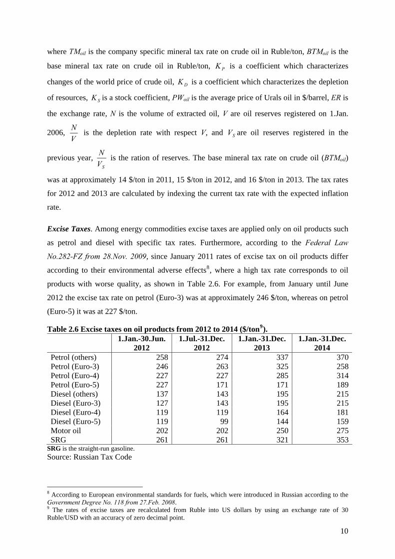
Excise Taxes. Among energy commodities excise taxes are applied only on oil products such

as petrol and diesel with specific tax rates. Furthermore, according to the Federal Law

No.282-FZ from 28.Nov. 2009, since January 2011 rates of excise tax on oil products differ

according to their environmental adverse effects8, where a high tax rate corresponds to oil

products with worse quality, as shown in Table 2.6. For example, from January until June

2012 the excise tax rate on petrol (Euro-3) was at approximately 246 $/ton, whereas on petrol

(Euro-5) it was at 227 $/ton.

Table 2.6 Excise taxes on oil products from 2012 to 2014 ($/ton9). 1.Jan.-30.Jun.

2012 1.Jul.-31.Dec.

2012 1.Jan.-31.Dec.

2013 1.Jan.-31.Dec.

2014 Petrol (others) 258 274 337 370Petrol (Euro-3) 246 263 325 258Petrol (Euro-4) 227 227 285 314Petrol (Euro-5) 227 171 171 189Diesel (others) 137 143 195 215Diesel (Euro-3) 127 143 195 215Diesel (Euro-4) 119 119 164 181Diesel (Euro-5) 119 99 144 159Motor oil 202 202 250 275SRG 261 261 321 353

SRG is the straight-run gasoline. Source: Russian Tax Code

8 According to European environmental standards for fuels, which were introduced in Russian according to the Government Degree No. 118 from 27.Feb. 2008. 9 The rates of excise taxes are recalculated from Ruble into US dollars by using an exchange rate of 30 Ruble/USD with an accuracy of zero decimal point.

10

3 Theoretical Background

According to the environmental taxation literature, an introduction of environmental taxes is

often related to the concept of double dividend, where substituting environmental taxes for

other distortionary taxes benefits not only the environment, but also reduces efficiency costs

of the tax system. A “weak” and “strong” double dividend hypothesizes are distinguished.

The relatively uncontroversial “weak” double dividend hypothesis argues that using revenues

from environmental taxes to reduce other distortionary taxes, one can achieve cost savings

(reductions in welfare costs of taxation) compared to the case where revenues are returned to

households in lump-sum form. The more ambiguous “strong” double dividend hypothesis

argues that not only can environmental welfare be increased but net welfare gains can be

achieved by alleviating pre-existing distortions (Goulder, 1994). The theoretical literature on

environmental taxation is mainly focused on pre-existing distortionary taxes in the labour and

capital market (Goulder et al. 1997; de Mooij and Bovenberg, 1998), whereas interactions

with other taxes such as imports and export taxes, valued added taxes, excise taxes, and

mineral resource extraction taxes are often neglected.

Using the analytical model developed by Goulder et al. (1997), and further modified to an

open economy model10 by Parry (2001), we analyze the welfare effect of pollution taxes.

Since the Russian economy strongly depends on revenues from export taxes on energy

resources, we extend the model framework by introducing an export tax on polluting

commodities. Household utility is given by the following equation:

)(),,( 21 HEvHCCuU , (3.1)

where u(*) is a utility function, which is quasi-concave and v(*) is a disutility function, which

is concave. Both functions are continuous. C1 is the domestic demand for the non-polluting

good 1, which is a composite of the domestically produced good (Q1) and the imported good

(M). The domestically produced and imported good 1 are treated as perfect substitutes (3.2).

C2 is the domestic demand for the polluting good 2, which is produced domestically only. The

domestic supply of good 2 (C2) is defined as the difference between the total supply (Q2) and

export (X), as given in equation (3.3). We consider the situation, where the country is an

exporter of the polluting good. H is leisure.

MQC 11 , (3.2)

. (3.3) XQC 22

10 To make it comparable, we keep the notation which is applied by Parry (2001).

11

We assume a small open economy, where the world price of the exported good (X) and the

world price of the imported good (M) are normalized at unity. Therefore, the trade account

balance is simply given by the following equation:

XM , (3.4)

Consumption of good 2 induces emissions. The environmental quality at home country (EH)

and abroad (EA) is defined by the following functions:

, (3.5) )( 2CeE HH

)(XeE AA . (3.6)

The marginal environmental damage (D) from consumption of good 2 (C2) in the home

country is measured in value terms. This can be derived using the disutility function in (3.1)

and (3.5):

2

1

C

e

e

vD H

H

, (3.7)

where is the marginal utility of income. We assume perfect competition and constant

returns to scale in the production of both goods, where labour is the only input. Therefore, the

marginal product of labour is constant, implying a perfectly elastic demand for labour.

Normalizing the wage rate and prices at unity, the economy resource constraint can be written

as follows:

, (3.8) HQQT 21

where T is the household time endowment. The total labour supply is the difference between

the time endowment and leisure: (T – H). Households are assumed to maximise the utility

(2.1) subject to the following household budget constraint:

TRHTCC LC ))(1()1( 221 , (3.9)

where 2C is the pollution tax on the good 2 (C2), L is the tax on labour income, and TR is

the total government revenue, which is returned to households as lump-sum transfers. The

total government revenue consists of revenues from pollution tax, labour tax, and export tax:

XHTCTR XLC )(22 , (3.10)

where X is the export tax. TR is exogenous in the model. This is because we analyse a

revenue neutral experiment, where the revenue from the pollution tax is recycled through a

12

reduction in the labour tax. Using this analytical framework, we can derive the following

propositions.

Proposition 1. The tax-interaction effect dominates the revenue-recycling effect, if 2C >0,

X =0, and C1 and C2 are equal substitutes for leisure.

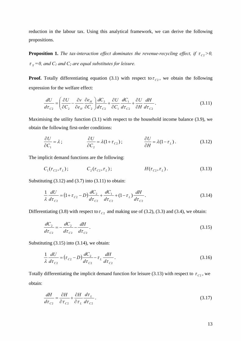
Proof. Totally differentiating equation (3.1) with respect to 2C , we obtain the following

expression for the welfare effect:

22

1

12

2

222 CCC

H

HC d

dH

H

U

d

dC

C

U

d

dC

C

e

e

v

C

U

d

dU

. (3.11)

Maximising the utility function (3.1) with respect to the household income balance (3.9), we

obtain the following first-order conditions:

1C

U; )1( 2

2CC

U

; )1( LH

U

. (3.12)

The implicit demand functions are the following:

),( 21 LCC ; ),( 22 LCC ; ),( 2 LCH . (3.13)

Substituting (3.12) and (3.7) into (3.11) to obtain:

22

1

2

22

2

)1(11

CL

CCC

C d

dH

d

dC

d

dCD

d

dU

. (3.14)

Differentiating (3.8) with respect to 2C and making use of (3.2), (3.3) and (3.4), we obtain:

22

2

2

2

CCC d

dH

d

dC

d

dC

. (3.15)

Substituting (3.15) into (3.14), we obtain:

22

22

2

1

CL

CC

C d

dH

d

dCD

d

dU

. (3.16)

Totally differentiating the implicit demand function for leisure (3.13) with respect to 2C , we

obtain:

222 C

L

LCC d

dHH

d

dH

. (3.17)

13

Totally differentiating the government revenue equation (3.10) with respect to 2C , after

some simple algebraic manipulation, gives

LL

CX

CL

CC

C

L

HHT

d

dXH

d

dCC

d

d

222

222

2

. (3.18)

Substituting (3.18) and (3.17) into (3.16), we can obtain:

222

222

2

22

2

)1(1

CL

CX

CC

CC

C

HM

d

dX

d

dCCM

d

dCD

d

dU

, (3.19)

where

LL

LL

HHT

H

M

. (3.20)

dWP ∂WR ∂WI

According to Goulder et al. (1997), the numerator in equation (3.20) defines the partial

equilibrium net welfare from a marginal change in the labour tax. This is the change in leisure

multiplied by L . The denominator defines the partial equilibrium change in government

revenues from a marginal change in the labour tax. Therefore, M is the partial equilibrium

efficiency costs11 resulting from an increase of labour tax to receive an additional dollar. The

first term in the RHS of the equation (3.19) is the Pigouvian effect, , which is defined as

a reduction of C2, multiplied by the difference between the marginal social benefit and the

marginal social cost. The revenue recycling effect is labeled by . The revenue-recycling

effect defines efficiency gains from a reduction of labour tax and gains from pollution tax

revenues. The tax interaction effect which is labeled by defines the welfare loss,

resulting from decreasing labour supply and revenues from labour taxes. The tax interaction

effect (∂WI) can be shown by the following approximation, which is derived following

Goulder et al. (1997) (see appendix A):

PdW

RW

IW

, where 2MCW CI

LIC

HCC

HC

LIC

HC

C

nCC

Cn

CC

Cn

nn

21

2

21

1

21

2 , (3.21)

11 According to Goulder et al. (1997), M is also defined as marginal excess burden of labour taxation, where one plus the marginal excess burden of taxation equals the marginal cost of public funds.

14

where and are the compensated elasticities of demand for C1, and C2 with

respect to the price of leisure, and is the income elasticity of labour supply. The degree of

substitution between C2 and leisure compared to that between total consumption and leisure is

measured by the term,

CHCn

1

CHCn

2

C

LIn

. For example, if C1 and C2 have equal elasticities of substitution for

leisure ( equals ), then CHCn

1

CHCn

2 X equals unity. Therefore, the difference between the

revenue-recycling effect ( ), and the tax-interaction effect ( ) equals: RW IW

22

22

CX

CC d

dX

d

dCM

. (3.22)

If 2C >0, X =0, then > by the termIW RW

2

22

CC d

dCM

. Q.E.D.

This confirms the conclusion made by Parry (1995) and Goulder et al. (1997) and implies a

failure of the strong double dividend hypothesis. The intuitive explanation for this is that

narrow-based taxes (pollution taxes) induce a larger marginal excess burden compared to

broad-based taxes (income taxes). Nevertheless, if pollution goods and leisure are

complements, the tax-interaction effect is an efficiency gain (Goulder et al. 1997). In addition,

Bovenberg and de Mooij (1994) show that the optimal pollution tax typically falls short of the

Pigouvian tax in the presence of tax distortions in the labour market. This means that

substituting pollution taxes for labour taxes exacerbate pre-existing distortions rather than

alleviate this.

Proposition 2. The tax-interaction effect is less than the revenue-recycling effect, if

0< 2C < X and C1 and C2 are equal substitutes for leisure.

Proof. Under the assumption of a small open economy and homogeneity of C2 and X in

supply, 2

2

CddC

=2Cd

dXwhere

2

2

CddC

<0 and 2Cd

dX2C>0. Therefore from (3.22), if < X , then

< . Q.E.D. I RW W

Expanding base of the export tax results in additional revenues, which allows for a larger

reduction in labour taxes. Such a positive tax-interaction effect decreases the cost of

environmental tax reform, raising the possibility of a strong double dividend.

15

Proposition 3. The tax-interaction effect equals the revenue-recycling effect, if 2C = X ,

X >0, and C1 and C2 are equal substitutes for leisure.

Proof follows from the proof of the Proposition 2, see equation (3.22). Q.E.D.

Using this analytical framework, we can also see that introducing (increasing) pollution taxes

harms the environmental quality abroad: 22 C

A

C

A

d

dX

Xd ede

<0 because X

e A

<0 and

2CddX

>0.

This indicates the emission leakage effect.

In addition, other important aspects of the double dividend hypothesis can be summarized as

follows:

(1) Williams12 (2002) analyses the link between pollution, human health, and labour

productivity. By using a modified version of the model developed by Parry et al.

(1999), he shows that introducing pollution taxes can improve health, resulting in

increases of labour productivity. This creates additional benefits from the

environmental tax reform, benefit-side tax-interaction effect, which can offset the

negative tax-interaction effect under certain conditions.

(2) Parry and Bento (2000)13 show that welfare gains from substituting environmental

taxes for labour taxes can be substantially larger, when tax-favoured consumption is

introduced in the model. This is because labour taxes distort also the choice among

consumption goods.

(3) In the presence of capital in the short and medium term, an environmental tax reform

can induce the so-called tax-shifting effect between factors. For example, if capital is

internationally mobile, substituting environmental taxes for capital taxes can yield a

double dividend, or if capital is internationally immobile, substituting environmental

taxes for labour taxes can reduce the efficiency costs of the tax system. Nevertheless,

in the long-run, capital is rather perfectly mobile. Therefore, under the assumption of

international capital mobility, an environmental tax reform can exacerbate rather than

alleviate initial inefficiencies in the tax system (de Mooij and Bovenberg, 1998).

(4) Apart from capital, natural resources can also be considered as a fixed factor. For

instance, Bento and Jacobsen (2007) show that in the presence of a fixed factor and

untaxable Ricardian rents, an environmental tax reform can induce a double dividend

12 In comparison, Williams (2003) considers the relationship between pollution and the health effect only. 13 For another special case see Parry and Bento (2001).

16

since the burden of environmental taxes is shared by labour and natural resources in

terms of lower prices of natural resources (Ricardian rents).

(5) According to Bovenberg and Ploeg (1998), important conditions under which an

environmental tax reform can increase employment are the following: low initial tax

rates on resources, a large production share of fixed factors, and high substitution

between labour and resources. The use of exhaustible resources, however, is often

subject for high taxes.

(6) Furthermore, there are other types of tax-shifting effects that can lead to a double

dividend such as tax-shifting across countries (terms of trade effect) and tax-shifting

among household incomes. For example, Killinger (1995) and de Mooij (1996) show

that the burden of environmental taxation can be partially shifted to foreign supplier

trough a terms-of-trade effect. This, however, is feasible only for large economies,

which can affect the world market price, exercising some market power.

A strong tax-shifting effect is the crucial condition for the occurrence of a strong double

dividend (de Mooij, 1996). In general, the occurrence of double-dividend effects is

ambiguous. The outcome, inter alia, depends on the tax and economic structure, household

preferences, factor mobility, factor substitution, and revenue recycling strategies. Hence

general equilibrium analysis is an appropriate analytical method (Goulder, 2002).

4 Numerical Model

4.1 Model and Database

The model is a modified version of the comparative static “STAGE” model (McDonald,

2007). The STAGE model is a member of the class of computable-general equilibrium (CGE)

models descended from the model described by Dervis et al. (1984) and more specifically the

USDA ERS model (Robinson et al., 1990; and Kilkenny, 1991). The model is a Social

Accounting Matrix (SAM) based single-country CGE model, which is implemented in

General Algebraic Modeling System (GAMS) software. For informal descriptions of the

model see appendix B.

This analysis is based on version 7 of the Global Trade Analysis Project (GTAP) database,

which represents the global economy in 2004. The GTAP database describes bilateral trade,

production, and consumption of 57 commodities and 113 regions (GTAP, 2007). The GTAP

database does not, however, include any enterprise accounts, and only one aggregated private

household is represented in the database. For our analysis we extract a Social Accounting

17

Matrix (SAM) for Russia using the GAMS version of the SAM extraction program developed

by McDonald and Thierfelder (2004). For this analysis, we aggregate 57 activities to 25

activities, where the SAM for Russia represents single product activities. The database

provides information on the main policy instruments such as import and export taxes,

consumption taxes, taxes on factor income, and taxes on factor use. According to the model

framework, commodity taxes are imposed on the final consumption as well as the

intermediate consumption. This, however, does not reflect the real system of value added

taxation in Russia. Under a value added tax system, which is applied in Russia as well as

many European countries, only the final consumption is taxed so that industries receive

rebates to avoid the cascading effect. Therefore, we can not draw any explicit conclusion with

respect to value added taxes; however, we can form plausible expectations based on changes

in final consumption. Furthermore, corporate income taxes are not explicitly depicted in the

database so that taxes on capital income include corporate income taxes, taxes on interest

from bank deposits and dividends.

CO2 coefficients are calculated based on the Energy Information Administration (EIA)

database (2011), by dividing the total CO2 emission of a certain energy product (measured in

million metric tons) by the total amount of energy used (measured in quadrillion Btu). Coal

and petroleum products contain the largest emission contents: for example, the CO2

coefficient for coal is 93 million metric tons per quadrillion Btu, petroleum products and

crude oil (67), natural gas, and gas manufacture (54). Moreover, following the GTAP

emission database (Lee, 2008), CO2 coefficients of coal, crude oil, and petroleum products

used by the petroleum sector equal zero. The same assumption is made for natural gas used by

gas manufacturing.

4.2 Experiments and Model Closures

In this analysis we simulate an introduction of carbon taxes on energy commodities such as

coal, natural gas, petroleum products, and gas manufacture used by households and industries.

Carbon taxation is not applicable for crude oil since crude oil is consumed mainly by the

petroleum sector. For instance, the share of crude oil consumption by the petroleum sector is

98% of domestic consumption (GTAP, 2007). The magnitude of carbon taxation aims at a

targeted reduction of carbon emissions by 10% through a proportional increase in tax rates on

carbon emissions. This means that carbon taxes differ between energy commodities according

to the CO2 coefficients, yet are the same among sectors and households. Revenues from

18

carbon taxes are recycled through a reduction in taxes on income from unskilled and skilled

labour. In the model we assume the following closure rules:

Foreign Exchange Closure. The external trade balance is fixed and the exchange rate is

flexible so that changes in the exchange rate clear the foreign exchange market;

Investment-Savings Closure. Volumes of investment are fixed and household savings rates

are variable so that the capital accounts are cleared by changes in the household savings rate.

The assumption of fixed investment is consistent with the long-run experiment;

Government Account Closure. Government savings rates and government consumptions are

fixed so that the government account is cleared by a reduction of labour taxes;

Numeraire. The consumer price index (CPI) is set as numeraire;

International Factor Mobility Closure. All factors are assumed to be internationally

immobile;

Factor Market Closure. Capital is assumed to be perfectly mobile among sectors; however,

we assume immobility of natural resources. Land is used by the agricultural sector only, and

hence it is a de facto immobile resource. Furthermore, we assume a perfectly elastic supply of

land. This is because Russia has a large potential for land resources – a lot of land remains

fallow. The supply of skilled and unskilled labour is assumed to be inelastic. We incorporate

supply functions for skilled and unskilled labour:

fefsffff TYFWFshfsFS ))1(*(* , (4.1)

where FSf is the supply of skilled and unskilled labour, shfsf is the shift parameter for the

supply function, WFf is the wage level, efsf is the labour supply elasticity which is assumed to

equal 0.30, following Böhringer et al. (2008)14, TYFf is the tax on factor income.

5 Results

Introducing carbon taxes results in welfare gains measured by equivalent variation15 (EV) of

2575 million USD or 0.9% of initial household expenditures. Household income increases by

1.3% because of higher income from land via an increase in supply of land as well as higher

income from increased skilled and unskilled labour via lower labour taxes and higher labour

supply. Moreover, the real GDP increases by 0.5%, accompanied by a depreciation of the

14 Evers et al. (2008) confirms this order of magnitude found that the mean labour supply elasticity for men equals 0.07, whereas for women it is 0.43. 15 Equivalent variation measures how much a consumer would pay before a price increase to avoid the price increase so that the income change is equivalent the price change regarding the utility change (Varian, 1999).

19

currency by 0.5%. Household expenditure – household income net of savings plus lump-sum

transfers – increases by 1.8%, which is stronger than the increase in household income

because of a lower savings rate, which falls by 1%. According to the model closures,

government savings, government consumption, and investment are fixed, which implies an

investment driven closure. Due to increasing household income, the savings rate decreases to

match fixed investment. Alternatively, if we fix the savings rate, investment in real terms

would increase because of higher household income; however, the increase in final

consumption would be less pronounced than it is under the investment driven closure.

Introducing carbon taxes compensated by a reduction in taxes on labour income leads to a

decrease of total government expenditures by 2.1% because of a decreasing price of public

services, whereas government consumption and savings are fixed. Government consumption

consists mainly of public services. As shown in Table 5.1, substituting carbon taxes for labour

taxes leads to increases in revenues from export, import and land taxes. In addition,

expenditures on production subsidies and transfers to households increase. In contrast,

revenues from taxes on factor income and consumption taxes decrease. The reasons for this

are explained further below.

Table 5.1 Changes of government revenues and expenditures from trade and domestic taxes (million USD and %). Absolute changes in

million USD Relative changes in

% Import taxes 54.89 0.56Export taxes 1037.30 4.05Consumption taxes -1624.12 -3.25Capital income taxes -706.94 -3.73Labour income taxes (unskilled labour) -10207.60 -33.86Labour income taxes (skilled labour) -4797.92 -34.09Land taxes 4.96 1.15SSC (unskilled labour) -153.74 -1.06SSC (skilled labour) -94.96 -1.41Mineral resource extraction taxes -86.65 -3.66Production subsidies 4.57 0.66Lump-sum transfers 1131.38 1.27Carbon taxes 15936.51 no

Source: model simulation results

Domestic Taxes. Substituting carbon taxes for taxes on labour earnings leads to increases in

supply of unskilled and skilled labour by 2.4% and 2.3%, respectively (Fig. 5.1). Increases in

labour supply indicate the so-called employment double dividend (Bovenberg and Ploeg,

1998). Due to tax incidence, gross wages for unskilled and skilled labour decreases by 3.3%

and 3.6%, respectively. Tax rates on earnings from unskilled and skilled labour decrease by

20

33.15% each. Both a reduction in labour tax rates and decreasing gross wages lead to

decreases in tax revenues from labour income: for example, revenues from taxes on unskilled

and skilled labour decrease by 33.9% and 34.1%, respectively. On the other hand, a reduction

in labour taxes as well as increasing labour supply alleviates distortions in the labour market.

Furthermore, even though supply of labour increases, the amount of social security

contributions from unskilled and skilled decreases by 1.1% and 1.4%, respectively, because of

decreasing gross wages.

Fig. 5.1 Changes of factor supply, factor prices, and revenues from factor taxes (%).

-33.9 -34.1

-3.8 -3.7

1.2

-3.3 -3.6 -3.8-6.9

2.4 2.3 1.2

-40

-35

-30

-25

-20

-15

-10

-5

0

5

USLab SLab Cap NatlRes Lnd

chan

ge

in %

Tax Revenues Factor prices Factor supply

USLab is unskilled labour; SLab is skilled labour; Cap is capital; NatlRes is natural resources; Lnd is land. Source: model simulation results

Introducing carbon taxes leads to decreases in demand for capital and natural resources,

resulting in decreases of returns to these factors. Decreasing prices of capital and natural

resources indicate a so-called tax-shifting effect (de Mooij and Bovenberg, 1998; Bento and

Jacobsen, 2007; Fraser and Waschik, 2010). This means that the burden of carbon taxes does

not fully pass on to final consumers, yet it is partially absorbed by lower factor prices.

According to the environmental taxation literature, the tax-shifting effect is an important

condition for the occurrence of a strong double dividend (de Mooij, 1996). Under the

assumption of a stock of capital and natural resources, changes of return to capital and

resources determine changing tax revenues. Due to decreasing returns to capital and natural

resources, revenues from taxes on capital income and mineral resource extraction taxes

decrease by about 3.7% each. In contrast, revenues from land taxes increase by 1.1% because

of increasing supply of land (Table 5.1).

Revenues from value added taxes and excise taxes are a significant part of the Russian

government budget. As discussed in section 4.1, we can not draw any explicit conclusion with

21

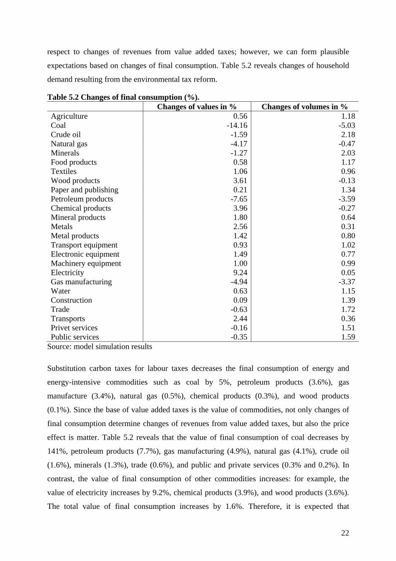
respect to changes of revenues from value added taxes; however, we can form plausible

expectations based on changes of final consumption. Table 5.2 reveals changes of household

demand resulting from the environmental tax reform.

Table 5.2 Changes of final consumption (%). Changes of values in % Changes of volumes in % Agriculture 0.56 1.18Coal -14.16 -5.03Crude oil -1.59 2.18Natural gas -4.17 -0.47Minerals -1.27 2.03Food products 0.58 1.17Textiles 1.06 0.96Wood products 3.61 -0.13Paper and publishing 0.21 1.34Petroleum products -7.65 -3.59Chemical products 3.96 -0.27Mineral products 1.80 0.64Metals 2.56 0.31Metal products 1.42 0.80Transport equipment 0.93 1.02Electronic equipment 1.49 0.77Machinery equipment 1.00 0.99Electricity 9.24 0.05Gas manufacturing -4.94 -3.37Water 0.63 1.15Construction 0.09 1.39Trade -0.63 1.72Transports 2.44 0.36Privet services -0.16 1.51Public services -0.35 1.59

Source: model simulation results

Substitution carbon taxes for labour taxes decreases the final consumption of energy and

energy-intensive commodities such as coal by 5%, petroleum products (3.6%), gas

manufacture (3.4%), natural gas (0.5%), chemical products (0.3%), and wood products

(0.1%). Since the base of value added taxes is the value of commodities, not only changes of

final consumption determine changes of revenues from value added taxes, but also the price

effect is matter. Table 5.2 reveals that the value of final consumption of coal decreases by

141%, petroleum products (7.7%), gas manufacturing (4.9%), natural gas (4.1%), crude oil

(1.6%), minerals (1.3%), trade (0.6%), and public and private services (0.3% and 0.2%). In

contrast, the value of final consumption of other commodities increases: for example, the

value of electricity increases by 9.2%, chemical products (3.9%), and wood products (3.6%).

The total value of final consumption increases by 1.6%. Therefore, it is expected that

22

revenues from value added taxes should increase because of increasing value of final

consumption. Excise taxes are imposed on commodities such as alcohol, cigarettes, cars, and

petroleum products. Introducing carbon taxes leads to increases in values of final

consumption of transport equipment by 0.9% and for food products16 it increases by 0.6%.

Therefore, we expect that revenues from excise taxes on alcohol, cigarettes, and transport

equipment should also increase. On the other hand, revenues from excise taxes on petroleum

products decrease, since the values of final consumption of petroleum products decreases by

7.6%.

Furthermore, the environmental tax reform leads to an increase in lump-sum transfers to

households by 1.3% because of increasing household income17. Expenditures on production

subsidies increase by 0.7%. The reason for this is an increase in agricultural production, since

only the agricultural sector receives production subsidies.

Trade Taxes. As shown in Fig. 5.2, the majority of revenues from export taxes come from

export taxes on crude oil, petroleum products, natural gas, and metals because of high tax

rates and high export supply. For example, the largest source of export revenues is export

taxes on crude oil, which amount to 69.6% of the total revenues from export taxes, followed

by petroleum products (9.2%), metals (6.9%), and natural gas (6.1%).

Fig. 5.2 Shares of several commodities in the total revenues from export taxes (%).

69.6

6.1

2.1

1.3

9.2

2.8

6.9

2.0

0 10 20 30 40 50 60 70 80

Oil

Natl.gas

Wood

Papers

Petrol

Chemical

Metals

Rest

shares in %

Source: version 7 of the GTAP database

Introducing carbon taxes leads to increasing exports of energy resources such as crude oil,

petroleum products, and natural gas. For example as shown in Table 5.3, export supply of

16 The demand category “food products” includes, inter alia, alcohol and cigarettes. 17 Household income is the base of lump-sum transfers.

23

crude oil increases by 5.6%, natural gas (14.3%), and petroleum products (3.5%). As a result,

revenues from export taxes on energy resources increase because of the expanding tax bases.

Moreover, the environmental tax reform leads to a depreciation of the currency by 0.5%,

which implies increasing export prices. Thus, both increasing export supply and a

depreciation of the currency leads to increasing revenues from export taxes.

Table 5.3 Changes of export tax revenues and export supply (million USD and %). Absolute changes

of export tax revenues in million

USD

Relative changes of export tax

revenues in %

Changes of export supply in %

Agriculture 0.06 3.72 3.13Coal -1.19 -4.36 -4.90Oil 1103.59 6.20 5.60Natural gas 155.19 9.95 14.32Minerals 6.52 3.94 3.35Textile product 5.22 4.69 4.10Wood products -99.75 -18.65 -19.11Paper and publishing 20.61 6.21 5.61Petroleum products 95.30 4.05 3.46Chemical products -110.17 -15.67 -16.14Mineral products -1.11 -2.61 -3.16Metals -141.58 -7.99 -8.52Metal products -0.16 -0.70 -1.26Transport equipment 3.79 6.23 5.63Electronic equipment -0.06 -1.04 -1.60Machinery equipment 1.04 1.40 0.83

Source: model simulation results

On the other hand, revenues from export taxes on metals, metal products, chemical products,

wood products, mineral products, coal, and electronic equipment decrease because of

decreasing export supply of these commodities. For example, export supply of metals

decreases by 8.5%, chemical products (16.1%), and wood products (19.1%). Because of a

deprecation of the currency, decreases in revenues from decreasing export supply are

diminished. Increases in revenues from export taxes on energy resources dominate decreases

in revenues from export taxes on other commodities. As a result, the total revenues from

export taxes increase by 4.1% (Table 5.1).

As shown in Fig. 5.3, the majority of revenues from imports tariffs come from import tariffs

on machinery equipment, food products, transport equipment, textiles, and chemical products,

because of high tariff rates and high import demand for these commodities. For example,

imports of machinery equipment is the largest source of revenues from import tariffs with a

24

share of 18% in the total revenue from import tariffs, followed by food products with a share

of 16.3%, transport equipment (15.4%), textiles (15%), and chemical products (12.5%).

Fig. 5.3 Shares of several commodities in the total revenues from import tariffs (%).

3.2

16.3

15.0

3.4

2.6

12.5

2.5

2.0

3.5

15.4

5.6

18.0

0 5 10 15 20

Agric.

Food

Textl.

Wood

Papers

Chemical

Min.prod.

Metals

Metal prod.

Trans.equ.

Elect.equ.

Mach.equ.

shares in %

Source: version 7 of the GTAP database

As shown in Table 5.4, introducing carbon taxes leads to increases in import demand for

electricity by 6.6%, wood products by 4.9%, chemical products (3.4%), electronic equipment

(0.4%), and metals (0.3%). This leads to increases in revenues from import tariffs on these

commodities. Similar to export taxes, increases (decreases) in revenues from imports tariffs

are increased (diminished) by a depreciation of the currency by 0.5%. Therefore, revenues

from import tariffs on textile and mineral products increase in spite of decreasing import

demand. On the other hand, revenues from import tariffs on other commodities decreases

because of decreasing import demand. Nevertheless, the bottom line is that the total revenues

from import tariffs increase by 0.6% (Table 5.1).

25

Table 5.4 Changes of import tax revenues and import demand (million USD and %). Absolute changes

of import tax revenues in million

USD

Relative changes of import tax

revenues in %

Changes of import demand in %

Agriculture -0.69 -0.22 -0.78Coal -0.22 -26.04 -26.45Oil -0.00 -16.86 -17.33Natural gas -0.00 -35.48 -35.84Minerals -0.76 -5.00 -5.54Food products -2.18 -0.14 -0.70Textile products 5.43 0.38 -0.19Wood products 18.10 5.51 4.92Paper and publishing -4.62 -1.86 -2.41Petroleum products -0.52 -14.65 -15.13Chemical products 48.05 3.98 3.40Mineral products 1.25 0.51 -0.05Metals 1.66 0.87 0.30Metal products -1.09 -0.32 -0.88Transport equipment -0.12 -0.01 -0.57Electronic equipment 5.25 0.97 0.41Machinery equipment -15.42 -0.89 -1.45Electricity 0.78 7.18 6.57

Source: model simulation results

6 Conclusions

Russia is not only a large source of carbon emissions, but is also one the most intensive users

of energy. Introducing carbon taxes would, potentially, address concerns on several fronts

simultaneously. In the short to medium term, they would reduce the emission of CO2 and

other emissions which are stemming from the use of energy commodities. In the longer term,

the increased costs of primary energy products should both accelerate the rate of technological

replacement and induce technological progress (Ruttan, 1997; Newell et al., 1999; Popp,

2002). In this paper, we analyze the incidence of carbon taxes as well as interactions of

carbon taxes with other taxes which are applied in Russia. Based on analytical and numerical

results, we can draw the following conclusions:

(1) Substituting carbon taxes for taxes on labour earnings in Russia leads an increase in

supply of unskilled and skilled labour by 2.4% and 2.3%, respectively, i.e. the so-

called employment dividend (Bovenberg and Ploeg, 1998);

(2) Under the assumption of international capital immobility, the burden of carbon taxes is

partially borne by capital in terms of decreasing capital income. In other words,

increasing energy costs do not fully pass on to final consumers. This indicates the so-

called tax-shifting effect (de Mooij and Bovenberg, 1998);

26

(3) Moreover, natural resources such as coal and natural gas also share the burden of

carbon taxation in terms of decreasing income from natural resources, which also

indicates the tax-shifting effect. This confirms to the conclusion made by Bento and

Jacobsen (2007) and Bovenberg and Ploeg (1998);

(4) The environmental tax reform leads to an increase in revenues from taxes on land

income because of expanding land supply by 1.2%;

(5) Revenues from export taxes increase by 1037.3 million USD or 4.1% because of

increases in export supply of natural gas, crude oil, petroleum products, minerals,

textiles, paper products, and transport and machinery equipment as well as a

depreciation of the currency;

(6) Revenues from import tariffs increase by 54.9 million USD or 0.6% because of

increases in revenues from import tariffs on wood products, textiles, chemical

products, metals, mineral products, metals, electronic equipment, and electricity

because of increasing import demand and currency depreciation;

(7) In addition, revenues from value added taxes as well as excise taxes on alcohol,

cigarettes, and transport equipment are expected to increase because of an increasing

value of final consumption;

However,

(8) Introducing carbon taxes leads to declining revenues from taxes on unskilled and

skilled labour by 10208 and 4798 million USD or about 34% each because of a

reduction of tax rates on labour income;

(9) Social security contributions from unskilled and skilled labour decline by 154 and 95

million USD or 1.0% and 1.4%, respectively, because of decreasing gross wages, even

though the employment increases;

(10) The environmental tax reform induces a reduction of revenues from taxes on capital

income by 707 million USD or 3.7% because of a decreasing return to capital. Taxes

on capital income include corporate income taxes, taxes on interest from bank deposits

and dividends;

(11) Revenues from taxes on mineral resource extraction decrease by 87 million USD or

3.7% because of a decreasing return to natural resources;

27

(12) Revenues from excise taxes on petroleum products decrease because of a decreasing

value of final consumption of petroleum products;

First of all, the model simulation results should be taken with caution since they are quite

sensitive to different parameters and assumptions. We find that substitution of carbon taxes

for labour taxes leads to welfare gains, yet this strongly depends on the labour supply

elasticity and elasticities of substitution between capital, energy and labour (Capros et al.,

1996; Sancho, 2010). This paper is aimed to show the relevance of interactions of carbon

taxes with other taxes. The main consideration behind this analysis is that increases

(decreases) in revenues from other taxes decrease (increase) the cost of environmental tax

reform. The analysis has some limitations. Other important issues that are behind the scope of

this analysis are carbon leakage effects and income inequality. Environmental tax reform can

induce large carbon leakages in countries that import Russian energy resources. Income

inequality is of high relevance in Russia. Carbon taxes are typically regressive; however,

substituting carbon taxes for labour taxes can redistribute income in favour of low and middle

income households, since the burden of taxation shifts from labour towards capital and natural

resources.

References

Bento, A., Jacobsen, M., 2007. Ricardian Rents, Environmental Policy and the ‘Double-Dividend’ Hypothesis. Journal of Environmental Economics and Management, 53 (2007), 17-31.

Böhringer, C., Löschel, A., Welsch, H., 2008. Environmental Taxation and Induced Structural Change in an Open Economy: The Role of Market Structure. German Economic Review, 9(1), 17-40.

Bovenberg, L., Goulder L., 1996. Optimal Environmental Taxation in the Presence of Other Taxes: General-Equilibrium Analyses. The American Economic Review, 86(4), 985-1000.

Bovenberg, A., and de Mooij, R., 1994. Environmental Levies and Distortionary Taxation. The American Economic Review, vol. 84. No. 4, 1085-1089.

Bovenberg, A., Ploeg., F., 1998. Environmental Policy, Public Finance and the Labour Market in a Second-Best World. Journal of Public Economics, 55 (1994), 349-390.

Burniaux, J-M., Truong, T., 2002. GTAP-E: An Energy-Environmental Version of the GTAP Model. GTAP Technical Paper No.16.

Burniaux, J-M., Martin, J.P., Nicolette, G., Martins, J.O., 1992. GREEN: A Multi-Sector, Multi-Region General Equilibrium Model for Quantifying the Costs of Curbing CO2 Emissions: A Technical Manual, OECD Department of Economics Working Papers No. 116. Paris: OECD

Capros, P., Georgakopulos, P., Zografakis, S., Proost, S., van Regemorter, D., Conrad, K., Schmidt, T., Smeers, Y., Michiels, E., 1996. Double Dividend Analysis: First Results of a General Equilibrium Model (GEM-E3) Linking the EU-12 Countries. Environmental Fiscal Reform and Unemployment. Kluwe Academic, 1996. pp. 193-227.

de Mooij, R., 1996. Environmental Taxation and the Double Dividend. Kluwe Academic, 1996. pp. 121-152.

de Mooij, R., Bovenberg, A., 1998. Environmental Taxes, International Capital Mobility and Inefficient Tax Systems: Tax Burden vs. Tax Shifting. International Tax and Public Finance, 5(1), 7-39.

EFA (Energy Forecasting Agency) 2009. Report: Operation and development of the Russian electric power industry. Available at: http://www.e-apbe.ru/analytical/

28

Evers, M., de Mooij, R., van Vuuren, D., 2008. The Wage Elasticity of Labour Supply: A Synthesis of Empirical Estimates. De Economist, 56, 25-43.

Fraser, I., Waschik, R. 2010. The Double Dividend Hypothesis in a CGE Model: Specific Factors and Variable Labour Supply. Working Paper No.2.

FSSS (Federal State Statistics Services) 2010. Financial Statistics 2004-2010. Available at: http://www.gks.ru/wps/wcm/connect/rosstat/rosstatsite/main/finance/

Goulder, L., 1994. Environmental Taxation and the “Double-Dividend”: A Reader’s Guide. International Tax and Public Finance, 2(2), 157-183.

Goulder, L., Parry, I., Burtraw, D., 1997. Revenue-Raising versus Other Approaches to Environmental Protection: The Critical Significance of Preexisting Tax Distortions. The RAND Journal of Economics, vol. 28 No. 4. pp. 708-731.

Goulder, L., 2002. Environmental Policy Making in Economies with Prior Tax Distortion. Cheltenham; Northampton, Mass.: Elgar: 2002: XXIII.

GTAP, 2007. Version 7 of the GTAP database.

Kilkenny, M., 1991. Computable General Equilibrium Modelling of Agricultural Policies: Documentation of the 30-Sector FPGE GAMS Model of the United States, USDA ERS Staff Report AGES 9125.

Killinger, S., 1995. Indirect Internalization of International Environmental Externalities. Discussion paper Nr.264. University of Konstanz.

Lee, H-L., 2008. An Emissions Data Base fro Integrated Assessment of Climate Change Policy Using GTAP. https://www.gtap.agecon.purdue.edu/resources/res_display.asp?RecordID=1143

Malcolm, G., 1998. Adjusting Tax Rates in the GTAP Data Base. GTAP Technical Paper No. 12.

McDonald, S., Thierfelder, K., 2004. Deriving a Global Social Accounting Matrix from GTAP Versions 5 and 6 Data. GTAP Technical Paper No. 22.

McDonald, S., 2007. A Static Applied General Equilibrium Model: Technical Documentation. STAGE Version 1: July 2007. Course documentation.

Newell, R., Jaffe, A., Stavins, R., 1999. The Induced Innovation Hypothesis and Energy-Saving Technological Change. Working Paper No. 6437.

Orlov, A., Grethe, H., McDonald, S. 2011. Energy Policy and Carbon Emission in Russia: A Short Run CGE Analysis. GTAP Conference Paper 2011.

Parry, I., 1995. Pollution Taxes and Revenue Recycling. Journal of Environmental Economics and Management 29, 64-77.

Parry, I., Williams, R., Goulder, L., 1999. When Can Carbon Abatement Policies Increase Welfare? The Fundamental Role of Distorted Factor Markets. Journal of Environmental Economics and Management, 37, 52-84.

Parry, I., 2001. The Costs of Restrictive Trade Policies in the Presence of Factor Tax Distortions. International Tax and Public Finance, 8, 147-170.

Parry, I., Bento, A., 2000. Tax Deductions, Environmental Policy, and the Double Dividend Hypothesis. Journal of Environmental Economics and Management, 39(1), 67-96.

Parry, I., Bento, A., 2001. Revenue Recycling and the Welfare Effects of Road Pricing. Scandinavian Journal of Economics, 103(4), 645-671.

Popp, D., 2002. Induced Innovation and Energy Prices. The American Economic Review, 92(1), 160-180.

Robinson, S., Kilkenny, M., Hanson, K., 1990. USDA/ERS Computable General Equilibrium Model of the United States, Economic Research Service, USDA, Staff Report AGES 9049.

Ruttan, V., 1997. Induced Innovation, Evolutionary Theory and Path Dependence: Sources of Technical Change. Economic Journal, 107(1997), 1520-1529.

Sancho, F., 2010. Double Dividend Effectiveness of Energy Tax Policies and the Elasticity of Substitution: A CGE Appraisal. Energy Policy, 38(6), 2927-2933.

Varian, H.R., 1999. Grundzüge der Mikroökonomik. 4. Auflage. Oldenbourg, 1999.

29

Williams III, R., 2002. Environmental Tax Interactions When Pollution Affects Health or Productivity. Journal of Environmental Economics and Management, 44, 261-270.

Williams III, R., 2003. Health Effects and Optimal Environmental Taxes. Journal of Public Economics, 87, 323-335.

Appendices

Appendix A: Derivation of Equation (3.21)

The tax-interaction effect ( ) is defined as following: IW

2

)1(C

LI H

MW

, (a1)

where

LL

LL

HHT

H

M

. (a2)

Substituting (a2) into (a1), we obtain:

2C

L

LL

I HH

HT

HTW

. (a3)

Multiplying by

L

L

H

H

yields:

L

CI

H

HHTM

W

2

)(

, (a4)

Making use of the Slutsky equation:I

HC

HH

C

C

C

222

and the Slutsky symmetry

property: L

C

C

C CH

2

2

, the term 2C

H

in the numerator of (a4) can be defined as

following:

I

HC

CH

L

C

C

22

2 , (a5)

where states for compensated and I is the disposable household income. c

30

Making use of the Slutsky equation, the term L

H

can be defined as following:

I

HHT

HH

L

C

L

)(

. (a6)

Differentiating time endowment constraint (3.8) with respect to L , we obtain:

L

C

L

C

L

C QQH

21 . (a7)

Substituting (a7) into (a6) gives:

I

HHT

QQH

L

C

L

C

L

)(21

. (a8)

Differentiating (3.2) and (3.3) with respect to L , we obtain:

L

C

L

C

L

CMCQ

11 , (a9)

L

C

L

C

L

CXCQ

22 . (a10)

Substituting (a9) and (a10) into (a8) to obtain:

I

HHT

CCH

L

C

L

C

L

)(21

. (a11)

Substituting (a5) and (a11) into (a4) gives:

I

HHT

CC

I

HC

CHTM

W

L

C

L

C

L

C

I

)(

)(

21

22

. (a12)

Equation (a12) can be rewritten as following:

))(1(

)(

)(

))(1()(

)1(

)1(

)1(

)1(

))(1(

)(

)(

))(1(

)1(

)1()(

2

2

21

1

1

22

2

2

HT

HT

HT

HT

I

HHT

C

C

CC

C

C

HT

HT

HT

HT

I

HC

C

C

CHTM

W

L

L

L

L

L

C

L

L

L

C

L

L

L

L

L

C

I

(a13)

Multiplying equation (a13) by L 1 gives:

)(

))((

212211

2212

CCnCnCn

nnCCMCW

LIHCC

HC

LIC

HCI

, (a14)

where

31

2

22

)1(

C

Cn L

L

CC

HC

; 1

11

)1(

C

Cn L

L

CC

HC

; )(

))(1(

HT

HT

I

Hn L

LI

. (a15)

Dividing by to obtain: )( 21 CC

LIHCC

HC

LIC

HCI

nCC

Cn

CC

Cn

nnMCW

21

22

21

11

22 )(, (a16)

or

, (a17) 2MCW CI

where

LIC

HCC

HC

LIC

HCC

nCC

Cn

CC

Cn

nn

21

22

21

11

2 )( . (a18)

Appendix B: Numerical Model

The standard “STAGE” model is extended by:

(1) Incorporating factor-fuel as well as inter-fuel substitution18 for non-energy producing

sectors;

(2) Incorporating a nested linear expenditure system for households, this distinguishes

between energy and non-energy composites;

(3) Disaggregating the electricity sector into four technologies: coal-fired, gas-fired,

nuclear, and hydro, using a technology bundle approach.

The main modifications19 relate to the production structure of the model follow a precedent

set by the GREEN model (Burniaux et al., 1992), and followed by other models, e.g., GTAP-

E (Burniaux and Truong, 2002), whereby energy inputs are nested with primary inputs to

form an energy-capital aggregate (QVKE). The production structure for non energy producing

sectors is illustrated in Fig. B1. Aggregate energy (QVE) is formed from electricity (QVEL)

and non electricity (QVNEL) with the latter being a two level aggregate from coal (QVCO)

and non-coal (QVNCO) where non coal energy sources are gas and oil based. Energy

producing sectors do not incorporate inter-fuel and factor-fuel substitutions. Elasticities of

substitution used are reported in Table B1.

18 A factor-fuel substitution is a substitution between energy inputs and primary factors. An inter-fuel substitution is a substitution among energy inputs (Burniaux and Truong, 2002). 19 Only informal descriptions of the model modification are provided here; for a formal description of the model see Orlov (2011)

32

Fig. B1 Production structure for non-energy producing sectors.

Source: own compilation

A slightly different production structure was used for gas and coal fired electricity generation

sectors. For these sectors the aggregate energy input (QVE) was derived as a single level

aggregate across the primary energy sources, while the preceding levels were left unchanged

from those reported in Figure A1; the elasticities are reported in Table B1. For the nuclear and

hydro electricity generating sectors there are no recorded inputs of primary energy sources but

electricity is used so the production structure effectively collapses so that the capital-energy

aggregate is an aggregate of capital and electricity.

33

Table B1 Elasticities of Substitution.

Non energy Energy Alternate Non

energy

X 0.5 0.5 0.5

VAE GTAP GTAP GTAP

VLL GTAP GTAP GTAP

VKE 0.0 0.0 0.0 or 0.5

VE 1.0 0.0 0.0 or 0.5

VNEL 0.5 na na

VNCO 1.0 na na

In addition the final demand system was modified by creating a two level demand system. At

the top level the household consumes two ‘commodities’ – energy and non energy – that

assumed to be aggregated with CES preferences (elasticity of substitution of 0.5). The energy

composite is also a CES aggregate (elasticity if substitution of 1.5) across all energy products

consumed by the household, while the non energy composite is a Cobb-Douglas aggregate

across all other commodities consumed by the household.

34

35

Appendix C: Elasticities in the Model

Table C1 Armington elasticities, CET elasticities, and elasticities of substitution among primary factors.

Armington elasticities

CET elasticities

Elasticities of substitution

among primary factors

Agriculture 1.45 1.50 0.22 Coal 1.52 0.50 0.20 Crude oil 2.60 3.00 0.20 Natural gas 8.60 3.00 0.20 Minerals 0.45 1.50 0.20 Food products 1.47 0.75 1.12 Textile products 1.91 1.50 1.26 Wood products 1.70 3.00 1.26 Paper products 1.47 1.50 1.26 Petroleum products 1.05 3.00 1.26 Chemical products 1.65 1.50 1.26 Mineral products 1.45 3.00 1.26 Metals 1.78 3.00 1.26 Metal products 1.87 3.00 1.26 Transport equipment 1.77 3.00 1.26 Electronic equipment 2.20 0.50 1.26 Machinery equipment 1.95 0.50 1.26 Electricity 1.40 0.50 1.26 Gas manufacture 1.40 0.50 1.26 Water 1.40 0.50 1.26 Construction 0.95 3.00 1.26 Trade 0.95 3.00 1.40 Transports 0.95 3.00 1.68 Private services 0.95 0.75 1.26 Government services 0.95 1.50 1.26

Source: Armington elasticities and elasticities of substitution among primary factors are from version 7 of the GTAP database; CET elasticities are assumed