Intro to Statistics for the Intro to Statistics for the Behavioral SciencesBehavioral Sciences

PSYC 1900PSYC 1900

Lecture 3: Central TendencyLecture 3: Central Tendency

And DispersionAnd Dispersion

Measures of Central Measures of Central TendencyTendency

Numerical values that refer to the Numerical values that refer to the center of a distributioncenter of a distribution Used to provide a “best descriptor” of Used to provide a “best descriptor” of

the score for a samplethe score for a sample Usefulness or quality of the measure Usefulness or quality of the measure

depends on shape of distributiondepends on shape of distribution

Mode, Median, and MeanMode, Median, and Mean

The ModeThe Mode

Defined as the Defined as the most common or most common or frequent scorefrequent score The value with the The value with the

highest point on a highest point on a frequency frequency distribution of a distribution of a variablevariable

3,4,1,5,7,1,2,3,1,1,63,4,1,5,7,1,2,3,1,1,6,1,7,2,1,7,2

The mode = 1The mode = 1

The ModeThe Mode

If two adjacent points occur with equal and If two adjacent points occur with equal and greatest frequency, the mode can be greatest frequency, the mode can be considered the average of these two.considered the average of these two.

Mode = 3.5Mode = 3.5

The ModeThe Mode If the two points are not adjacent and If the two points are not adjacent and

equal, the distribution is bimodal.equal, the distribution is bimodal. Of course, binning might result in a single mode Of course, binning might result in a single mode

by eliminating error/noise.by eliminating error/noise. Bimodal usually means substantially separatedBimodal usually means substantially separated

The MedianThe Median Score that corresponds to the point at Score that corresponds to the point at

or below which 50% of scores fallor below which 50% of scores fall The “middle” number in a ranking of the The “middle” number in a ranking of the

datadata Median LocationMedian Location

Mdn location = (N+1)/2Mdn location = (N+1)/2 If we have 11 numbers, the mdn location is:If we have 11 numbers, the mdn location is:

(11+1)/2 = 6(11+1)/2 = 6 1,1,2,3,3,3,4,4,5,5,61,1,2,3,3,3,4,4,5,5,6 Mdn = 3Mdn = 3

The MedianThe Median

What about: 1,1,2,3,3,3,4,4,5,5,6,6What about: 1,1,2,3,3,3,4,4,5,5,6,6 Mdn location = (12+1) / 2 = 6.5Mdn location = (12+1) / 2 = 6.5 Mdn = 3.5Mdn = 3.5

When the median location falls between When the median location falls between points, the median is defined as the points, the median is defined as the average of those two points.average of those two points.

Median: Histogram vs. Stem Median: Histogram vs. Stem and Leafand Leaf

Stem-and-Leaf Plot

Frequency Stem & Leaf

2.00 1 . 00 1.00 2 . 0 3.00 3 . 000 2.00 4 . 00 2.00 5 . 00 2.00 6 . 00

Stem width: 1.00 Each leaf: 1 case(s)

The MeanThe Mean

The average valueThe average value The sum of the scores divided by the number The sum of the scores divided by the number

of scoresof scores

2,4,5,9,112,4,5,9,11 (2+4+5+9+11)=31; 31/5=6.2(2+4+5+9+11)=31; 31/5=6.2

XX

N

Relations Among Measures of Relations Among Measures of Central TendencyCentral Tendency

When the When the distributions are distributions are symmetric, the symmetric, the three measures will three measures will generally generally correspond.correspond.

When the When the distributions are distributions are asymmetric, they asymmetric, they will often diverge.will often diverge.

Score

2.832.43

2.031.63

1.23.83

.43.03

-.37-.77

-1.17-1.57

-1.98-2.38

-2.78

20

10

0

Std. Dev = 1.02

Mean = -.01

N = 200.00

The Mode:The Mode:Advantages & DisadvantagesAdvantages & Disadvantages

Mode is the most commonly occurring Mode is the most commonly occurring score.score. Always appears in the data; mean and median Always appears in the data; mean and median

may not.may not. Most likely score to occur.Most likely score to occur. Useful for nominal data; mean and median are Useful for nominal data; mean and median are

not.not.

When might the mode be useful?When might the mode be useful?

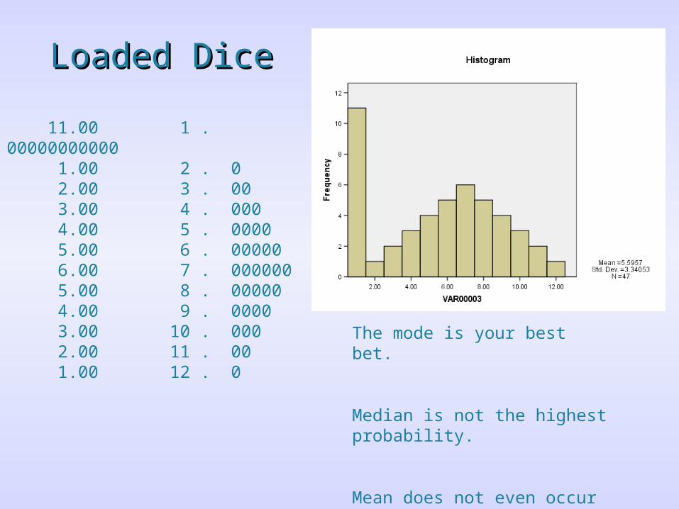
Loaded DiceLoaded Dice

The mode is your best bet.

Median is not the highest probability.

Mean does not even occur in sample.

11.00 1 . 00000000000 1.00 2 . 0 2.00 3 . 00 3.00 4 . 000 4.00 5 . 0000 5.00 6 . 00000 6.00 7 . 000000 5.00 8 . 00000 4.00 9 . 0000 3.00 10 . 000 2.00 11 . 00 1.00 12 . 0

Disadvantages of The ModeDisadvantages of The Mode

Mode can vary depending on how Mode can vary depending on how data are grouped/binneddata are grouped/binned

May not be representative of entire May not be representative of entire distributiondistribution Loaded Dice ExampleLoaded Dice Example Rare events (e.g., most frequent is zero)Rare events (e.g., most frequent is zero)

Tells us nothing about cause of nonzero Tells us nothing about cause of nonzero eventsevents

Advantages & DisadvantagesAdvantages & Disadvantagesof the Mean and Medianof the Mean and Median

Let me tell you a story . . . .Let me tell you a story . . . .

Better known as ALWAYS look Better known as ALWAYS look at your data distributionsat your data distributions

Men, Women, Evolution, & Men, Women, Evolution, & SexSex

Is there a gender difference in the Is there a gender difference in the number of desired partners?number of desired partners?

Evolutionary psychologists say “yes” Evolutionary psychologists say “yes” due to an asymmetry in minimum due to an asymmetry in minimum parental investment needs.parental investment needs.

Data appeared to support thisData appeared to support this

Men, Women, Evolution, & Men, Women, Evolution, & SexSex

Mean # partners in next 30 years:Mean # partners in next 30 years: Men = 7.69; Women = 2.78Men = 7.69; Women = 2.78

You can’t blame men; it’s in there You can’t blame men; it’s in there nature!nature!

Yes? No? Any ideas?Yes? No? Any ideas?

Means versus MediansMeans versus Medians These folks never considered the form of These folks never considered the form of

their data (or did they?)their data (or did they?) Without winsorization, men’s mean = 64Without winsorization, men’s mean = 64

Means: Men = 7.69; Women = 2.78Means: Men = 7.69; Women = 2.78

Medians and Modes = 1Medians and Modes = 1

Advantages & DisadvantagesAdvantages & Disadvantagesof the Mean and Medianof the Mean and Median

Mean is subject to bias by extreme valuesMean is subject to bias by extreme values May provide a value for central tendency that May provide a value for central tendency that

does not exist in data setdoes not exist in data set Major benefit is historical use and ability to Major benefit is historical use and ability to

be manipulated algrebraically be manipulated algrebraically Most mathematical equations depend on itMost mathematical equations depend on it When assumptions are met, it is quite validWhen assumptions are met, it is quite valid

MedianMedian Not influenced by extreme values (e.g., Not influenced by extreme values (e.g.,

salaries, home values).salaries, home values). Not as amenable to algebraic manipulation and Not as amenable to algebraic manipulation and

use.use.

Measures of Measures of Variability/DispersionVariability/Dispersion

The degree to which individual data The degree to which individual data points are distributed around the meanpoints are distributed around the mean

Provide a measure of how representative Provide a measure of how representative the mean is of the scores the mean is of the scores

More Representative

Several MeasuresSeveral Measures RangeRange

Distance from lowest to highest valuesDistance from lowest to highest values 1,2,3,4,4,5,6,7; Range = 7-1 = 61,2,3,4,4,5,6,7; Range = 7-1 = 6 Suffers from sensitivity to extremesSuffers from sensitivity to extremes

1,2,3,4,4,5,6,7,80; Range = 80-1 = 791,2,3,4,4,5,6,7,80; Range = 80-1 = 79

Interquartile RangeInterquartile Range Range of the middle 50% of scoresRange of the middle 50% of scores Less dependent on extreme valuesLess dependent on extreme values

Trimmed samples and statisticsTrimmed samples and statistics

Average DeviationAverage Deviation

Conceptually ClearConceptually Clear How far individual scores deviate from How far individual scores deviate from

the mean on averagethe mean on average Problem is that average deviation from Problem is that average deviation from

the mean is, be definition, zerothe mean is, be definition, zero 1,2,3,3,4,51,2,3,3,4,5 Deviations: -2,-1,0,0,1,2Deviations: -2,-1,0,0,1,2 Average Deviation = 0Average Deviation = 0

The VarianceThe Variance

Solves the problem that deviations sum to Solves the problem that deviations sum to zerozero

Variance is defined as the average of the Variance is defined as the average of the sum squared deviations about the meansum squared deviations about the mean Squares of negative numbers are positiveSquares of negative numbers are positive Divide by N-1, not NDivide by N-1, not N

Sample Variance is used to estimate Sample Variance is used to estimate Population VariancePopulation Variance

The VarianceThe Variance

2

2 1

( )

1

n

ii

x

X Xs

N

Data: 1,2,3,3,4,4,4,5,6

Volunteer?

Descriptives

3.55562.3955

4.7157

3.56174.00002.278

1.509231.006.005.002.00

MeanLower BoundUpper Bound

95% ConfidenceInterval for Mean

5% Trimmed MeanMedianVarianceStd. DeviationMinimumMaximumRangeInterquartile Range

VAR00001Statistic

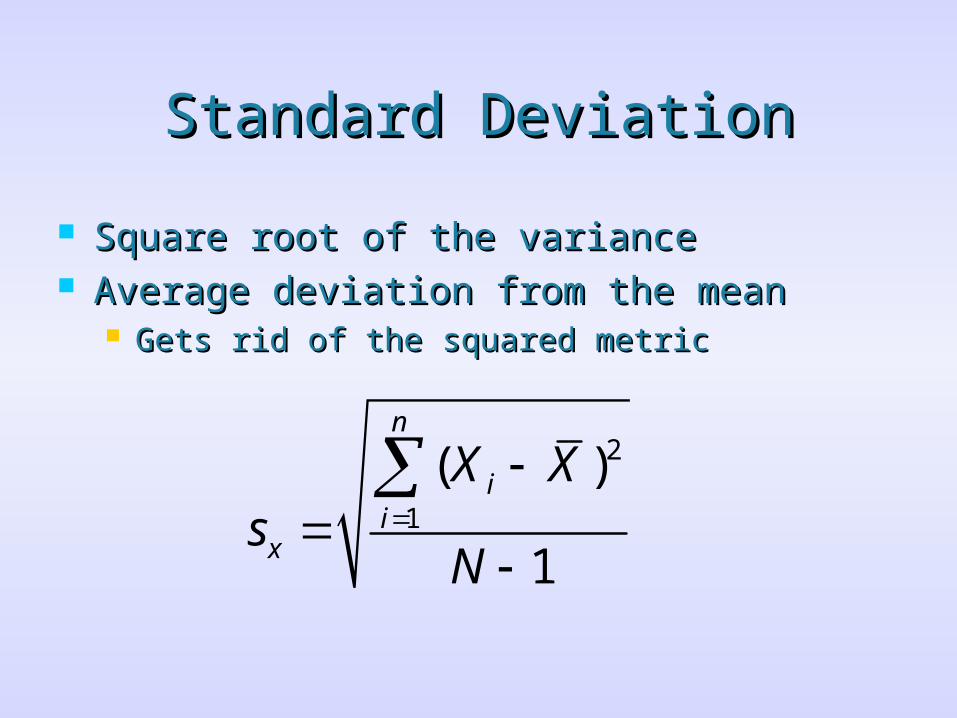
Standard DeviationStandard Deviation

Square root of the varianceSquare root of the variance Average deviation from the meanAverage deviation from the mean

Gets rid of the squared metricGets rid of the squared metric

2

1

( )

1

n

ii

x

X Xs

N

Computational FormulaeComputational Formulae

Algebraic manipulations are less clear Algebraic manipulations are less clear conceptually but easy to useconceptually but easy to use

2

2

2

2

2

1

1

X

X

XX

NsN

XX

NsN

Mean and Variance as Mean and Variance as EstimatorsEstimators

These descriptive statistics are used to These descriptive statistics are used to estimate parametersestimate parameters

XX

2 2X Xs

Bias in Sample VarianceBias in Sample Variance

If we calculated the average squared If we calculated the average squared deviation of the sample (as opposed to deviation of the sample (as opposed to dividing by N-1), the variance would be a dividing by N-1), the variance would be a biased estimate of the population biased estimate of the population variance.variance.

Bias: A property of a statistic whose long-Bias: A property of a statistic whose long-range average is not equal to the parameter range average is not equal to the parameter it estimates.it estimates.

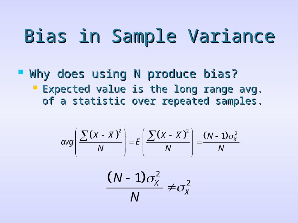
Bias in Sample VarianceBias in Sample Variance

Why does using N produce bias?Why does using N produce bias? Expected value is the long range avg. of a Expected value is the long range avg. of a

statistic over repeated samples.statistic over repeated samples.

2 2 21 X

X X X X Navg E

N N N

221 XX

N

N

Applet ExampleApplet Example

Multiply by constant: N/N-1Multiply by constant: N/N-1

2 21 X

X X NE

N N

2 2

2

2

1

1 1

1

X

X

X X NN NE

N N N N

X XE

N

Box-and-Whisker PlotsBox-and-Whisker Plots

Graphical representations of Graphical representations of dispersiondispersion

Quite useful to quickly visualize Quite useful to quickly visualize nature of variability and extreme nature of variability and extreme scoresscores

Box-and-Whisker PlotsBox-and-Whisker Plots

First find the median location and mdnFirst find the median location and mdn Find the quartile locationsFind the quartile locations

Medians of the upper and lower half of Medians of the upper and lower half of distributiondistribution

Quartile location = (mdn location + 1) / 2Quartile location = (mdn location + 1) / 2 These are termed the “hinges”These are termed the “hinges” Note: drop fractional values of mdn locationNote: drop fractional values of mdn location Hinges bracket interquartile range (IQR)Hinges bracket interquartile range (IQR) Hinges serve as top and bottom of boxHinges serve as top and bottom of box

Box-and-Whisker PlotsBox-and-Whisker Plots Find the H-spreadFind the H-spread

Range between two quartilesRange between two quartiles Simply the IQRSimply the IQR Area inside box in plotArea inside box in plot

Draw the whiskersDraw the whiskers Lines from hinges to farthest points not Lines from hinges to farthest points not

more than 1.5 X H-spreadmore than 1.5 X H-spread OutliersOutliers

Points beyond whiskersPoints beyond whiskers Denoted with asterisksDenoted with asterisks

Box-and-Whisker PlotsBox-and-Whisker PlotsStem-and-Leaf Plot

Frequency Stem & Leaf

2.00 0 . 11 3.00 0 . 223 3.00 0 . 445 6.00 0 . 667777 3.00 0 . 889 1.00 Extremes (>=15)

Stem width: 10.00 Each leaf: 1 case(s)

ExampleExample