intro to microsoft excel 2010 to microsoft excel 2010 . ... maximum value of selected numbers. you...

Intro to Microsoft Excel 2010

City of Los Angeles ● Department of Recreation and Parks

Introduction to Microsoft Excel 2010

Class Description: Students will be introduced to MS Excel 2010, a spreadsheet program that can organize

and analyze data for business and/or personal use. Basic skills taught are worksheet

navigation, data entry, chart and graphs, formatting, and Excel functions. This class is

targeted at beginning students who have never used Excel however a prerequisite is

the ability to use a mouse and some basic experience with Windows.

Introduction: MS Excel 2010 is an application that allows the user to keep track of and organize data

on a worksheet similar to an accounting ledger. The worksheet pages have columns

and rows which can be filled with text, numbers, dates, times, dollar amounts,

percentages, formulas, and more. The program can automatically calculate totals and

organize the information you have input. The calculations and information can be

presented in various types of charts and graphs. This will not only make your data look

professional but will also convey the information clearly. There are several uses for MS

Excel 2010, such as creating a checklist, a budget, an inventory, or a schedule. During

this training, you will learn how to use Excel to help you sort through, manage, and

organize data. By the end of this course, you will be able to:

Objectives: Perform basic navigation to effectively use the Microsoft Excel program.

Create and edit a simple spreadsheet.

Format the spreadsheet and perform calculations.

Preview, print, save, and open files.



Table of Contents Understanding MS Excel 2010 Basics ……………………………………………... 5

What is Microsoft Excel? ……………………………………………………….. 6

Accessing Microsoft Excel ………………………...………………………….... 7

Explore Excel ………..………………………………………………………….. 8

Creating a Simple Worksheet ……………………………………………………….. 15 Moving Around a Worksheet …………………………………………………… 16

Select Cells ………………………………………………………………………. 20

Enter Data ………………………………………………………………………... 22

Edit a Cell ……………………………………………………………………….... 23

Wrap Text ………………………………………………………………………… 25

Copy, Cut, Paste ………………………………………………………………… 26

Columns and Rows ……………………………………………………………… 29

New Worksheet ………………………………………………………………….. 31

Save Your Worksheet…………………………………………………………… 32

Close Open and Exit ……………………………………………………………. 33

Basic Formats and Formulas …………………………………………………………34 Borders ………………………………………………………………………….... 36

Merge and Center ………………………………………………………………. 38

Background Color ………………………………………………………………. 39

Font Formats – Styles, Size and Color ……………………………………….. 40

Bold, Italicize and Underline …………………………………………………… 42

Text Alignment …………………………………………………………………… 43

Format Numbers ………………………………………………………………… 44

Perform Mathematical Calculations …………………………………………… 46

AutoSum …………………………………………………………………………. 50

Creating a Chart ………………………………………………………………………... 52 Create a Chart ………………………………………………………………….... 53

Chart Layouts and Displays ……………………………………………………. 55



http://www.baycongroup.com/excel2007/02_excel.htm










Chart Styles – Color, Format, and Type ………………………………………. 57

Preview and Print Your Work ……………………………………………………...… 60 Page Layout ……………………………………………………………………… 61

Print Preview and Print …………………………………………………………. 63

Getting Help …………………………………………………………………….... 64

Quick Reference Guide ……………………………………………………………….. 65

Keyboard Shortcuts ……………………………………………………………... 66

Glossary ………………………………………………………………………….. 67

References ……………………………………………………………………….. 71



Lesson 1: Understanding Excel Basics


5 City of Los Angeles ● Department of Recreation and Parks

1A: What is Microsoft Excel?

Microsoft Excel is a spreadsheet program that allows a person to keep track and

organize data on a spreadsheet. It provides on the screen a page that looks like a

table, graph paper, or an accounting ledger in which the user can type numbers or

information in each square. Once data is entered on the worksheet, users have the

ability to build models for analyzing data, perform calculations with numbers, and

present data in 3D charts and graphs.

What Can You Use MS Excel 2010 For? MS Excel 2010 is not only used for managing data for businesses, but can also be used

for practical, everyday tasks, including:

Manage your finances. Set up a budget to track your monthly income and

expenses. Build a spreadsheet that helps you plan and track your savings

for retirement, your child's college education, or keep track of sales income

for your small business.

Create a calendar or schedule. Make a personal daily appointment

planner; or a schedule for managing homework, dinner, or bill payments.

Plan an event or organize a project. Keep track of multiple tasks and

deadlines, as well as schedules of other participants.

Create various types of lists such as checklists, phone lists, grocery lists,

etc.



http://www.ehow.com/how_4606589_what-some-practical-uses-excel.html

http://www.ehow.com/business/

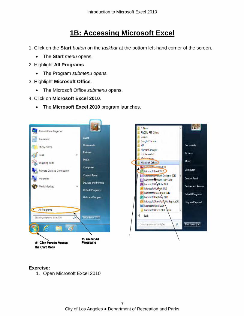
1B: Accessing Microsoft Excel

1. Click on the Start button on the taskbar at the bottom left-hand corner of the screen.

4. Click on Microsoft Excel 2010.

• The Microsoft Excel 2010 program launches.

Exercise: 1. Open Microsoft Excel 2010

• The Start menu opens.

2. Highlight All Programs.

• The Program submenu opens.

3. Highlight Microsoft Office.

• The Microsoft Office submenu opens.

#3 Click on Microsoft Office to open the submenu.

#4 Select Microsoft Excel 2010 by double clicking on it.



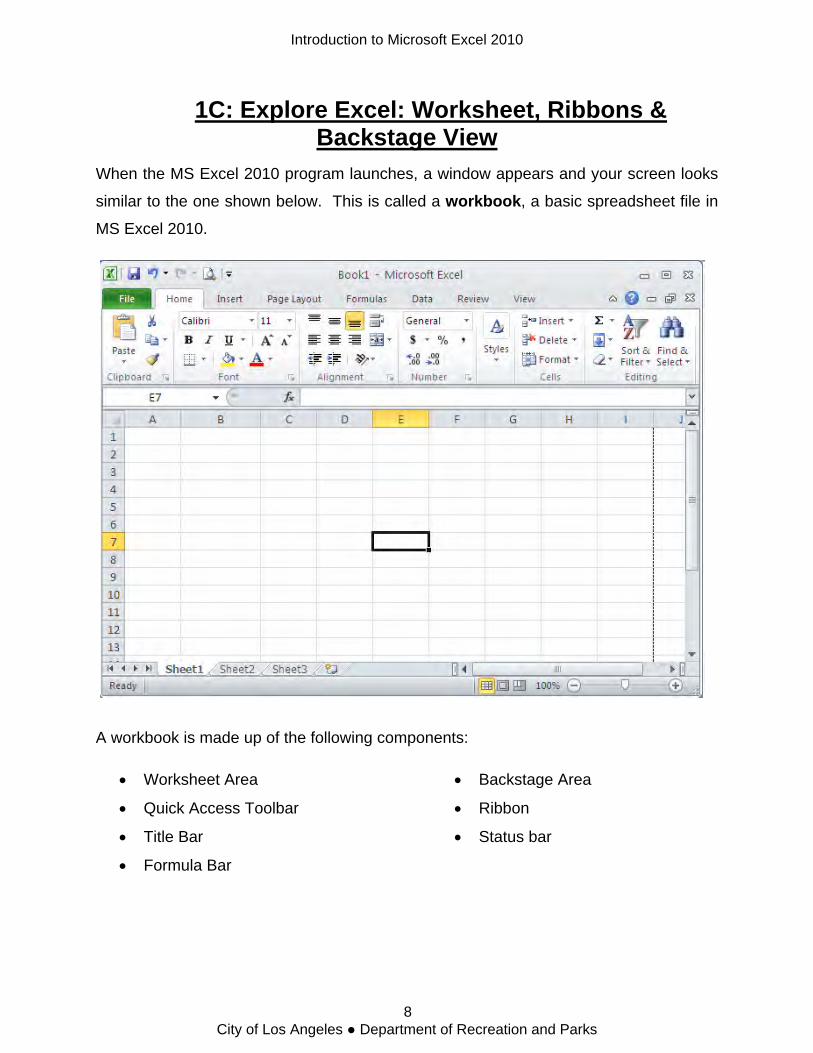
1C: Explore Excel: Worksheet, Ribbons & Backstage View

When the MS Excel 2010 program launches, a window appears and your screen looks

similar to the one shown below. This is called a workbook, a basic spreadsheet file in

MS Excel 2010.

A workbook is made up of the following components:

• Worksheet Area • Backstage Area

• Quick Access Toolbar • Ribbon

• Title Bar • Status bar

• Formula Bar



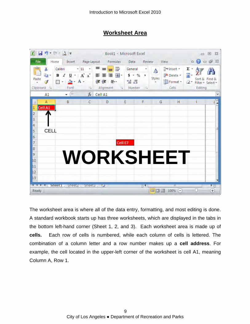
Worksheet Area

CELL

WORKSHEET

The worksheet area is where all of the data entry, formatting, and most editing is done.

A standard workbook starts up has three worksheets, which are displayed in the tabs in

the bottom left-hand corner (Sheet 1, 2, and 3). Each worksheet area is made up of

cells. Each row of cells is numbered, while each column of cells is lettered. The

combination of a column letter and a row number makes up a cell address. For

example, the cell located in the upper-left corner of the worksheet is cell A1, meaning

Column A, Row 1.



The Ribbon

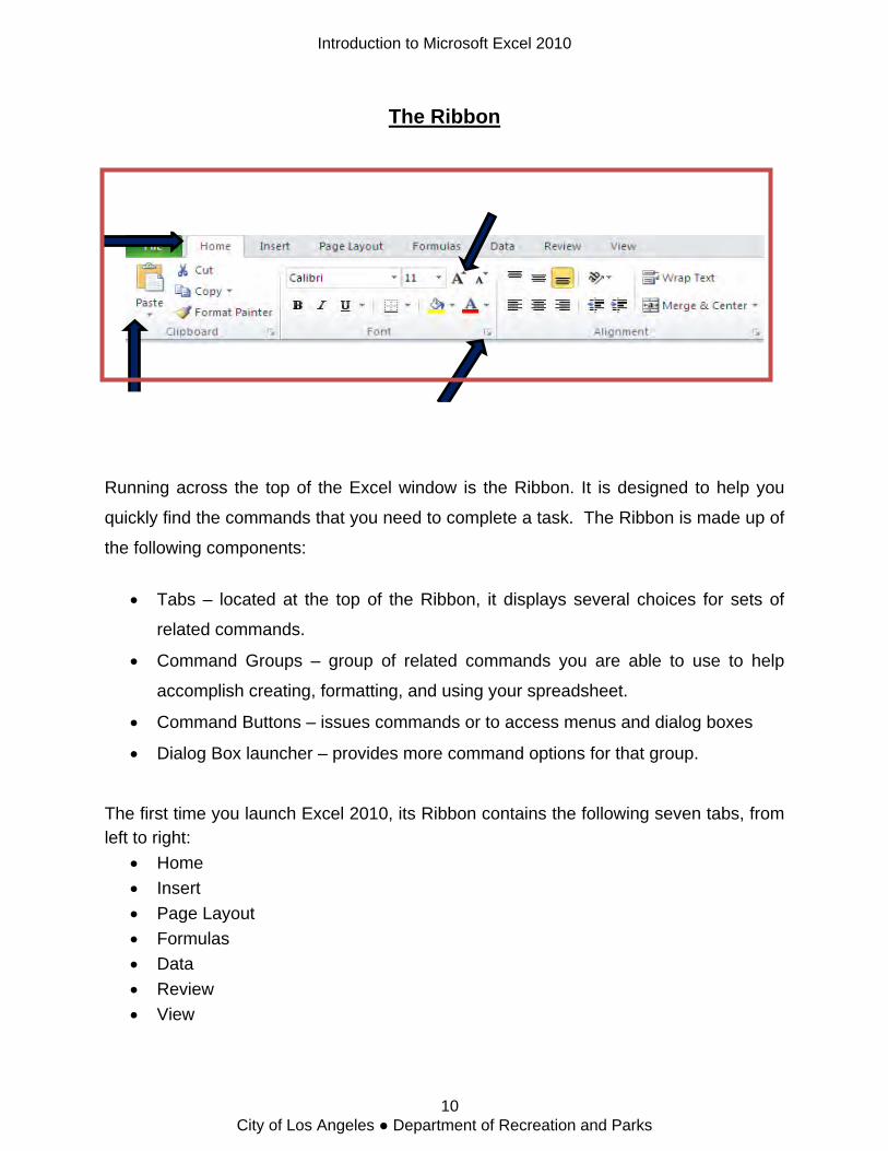
Running across the top of the Excel window is the Ribbon. It is designed to help you

quickly find the commands that you need to complete a task. The Ribbon is made up of

the following components:

• Tabs – located at the top of the Ribbon, it displays several choices for sets of

related commands.

• Command Groups – group of related commands you are able to use to help

accomplish creating, formatting, and using your spreadsheet.

• Command Buttons – issues commands or to access menus and dialog boxes

• Dialog Box launcher – provides more command options for that group.

The first time you launch Excel 2010, its Ribbon contains the following seven tabs, from left to right:

• Home • Insert • Page Layout • Formulas • Data • Review • View



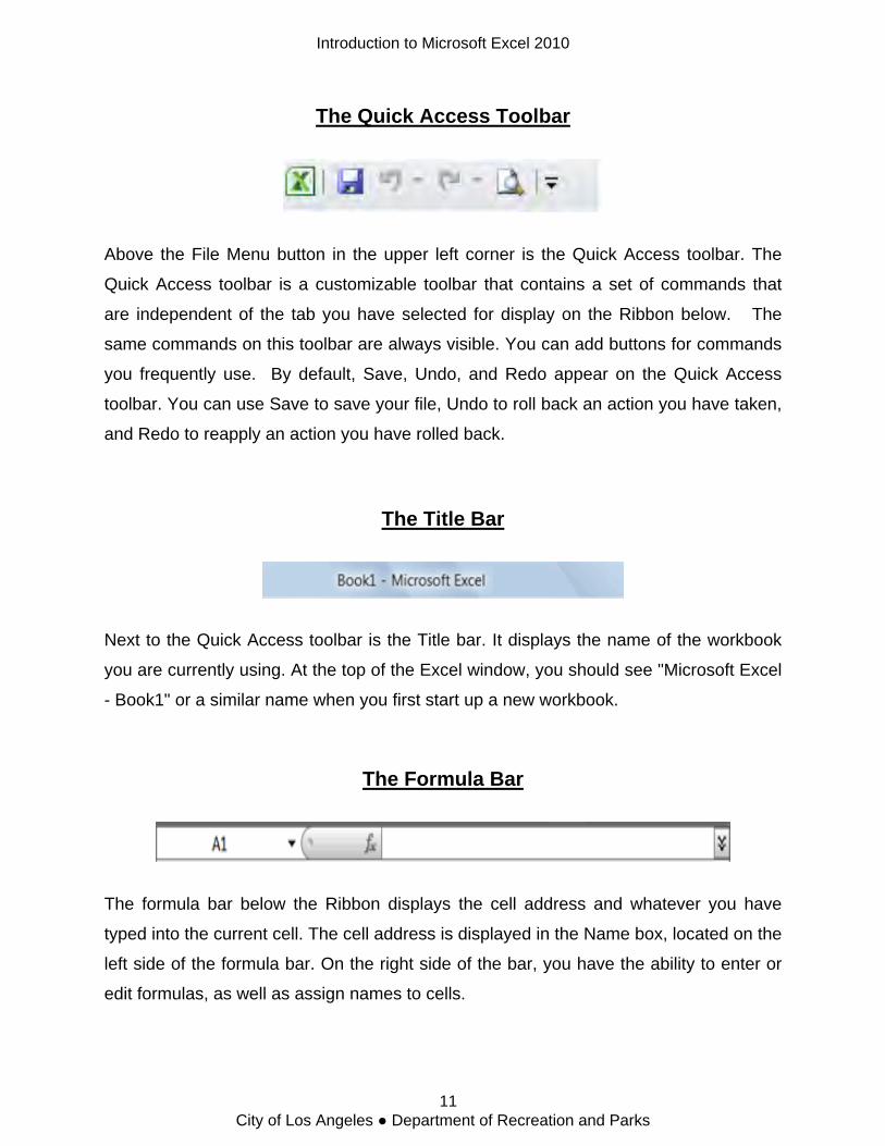
The Quick Access Toolbar

Above the File Menu button in the upper left corner is the Quick Access toolbar. The

Quick Access toolbar is a customizable toolbar that contains a set of commands that

are independent of the tab you have selected for display on the Ribbon below. The

same commands on this toolbar are always visible. You can add buttons for commands

you frequently use. By default, Save, Undo, and Redo appear on the Quick Access

toolbar. You can use Save to save your file, Undo to roll back an action you have taken,

and Redo to reapply an action you have rolled back.

The Title Bar

Next to the Quick Access toolbar is the Title bar. It displays the name of the workbook

you are currently using. At the top of the Excel window, you should see "Microsoft Excel

- Book1" or a similar name when you first start up a new workbook.

The Formula Bar

The formula bar below the Ribbon displays the cell address and whatever you have

typed into the current cell. The cell address is displayed in the Name box, located on the

left side of the formula bar. On the right side of the bar, you have the ability to enter or

edit formulas, as well as assign names to cells.



Backstage Area

Near the top-left corner of the MS Excel 2010 window is the green File tab. This is

where you can access the Backstage Area, which contains document- and file-related

commands: Info, Save, Save As, Open, Close, Recent, New, Print, and Save & Send. In addition, there is a link to get Help. Options enable you to change many of

Excel’s default settings, and Exit quits the program.

To close the Backstage view and return to the normal worksheet view, you can click the

File tab again or simply press the Escape (Esc) key.



http://www.dummies.com/how-to/content/using-excel-2010s-file-tab-to-access-backstage-vie.html#glossary-worksheet

Quick Guide to Excel Windows

The table below is a quick guide to finding some of the common items that you might be

using in MS Excel 2010 from the File tab or tabs on the Ribbon.

To: Click: Then Look in the….

Create, open, save, print, preview, protect, send, or

convert file

File Backstage view (click the links on the

left side in this view)

Insert, delete, format, or find data in cells, columns,

and row

Home Number, Styles, Cells, and Editing

ribbon groups

Add PivotTables, Excel tables (formerly lists), charts,

sparklines, hyperlinks, or headers and footers

Insert Tables, Charts, Sparklines, Links, and

Text ribbon groups

Set page margins and page breaks, specify print

area, or repeat rows

Page Layout

Page Setup and Scale to Fit ribbon

groups

Find functions, define names, or troubleshoot

formulas

Formulas Function Library, Defined Names, and

Formula Auditing ribbon groups

Import data, connect to a data source, sort data, filter

data, validate data, or perform a what-if analysis

Data Get External Data, Connections, Sort &

Filter and Data Tools ribbon groups

Check spelling, review and revise, or protect a

workbook

Review Proofing, Comments, and Changes

ribbon groups

Switch between worksheet views or active

workbooks, arrange windows, freeze panes, or

record macros

View Workbook Views, Window, and Macros

ribbon groups



The Status Bar

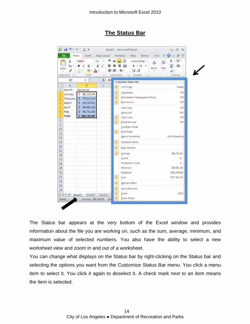
The Status bar appears at the very bottom of the Excel window and provides

information about the file you are working on, such as the sum, average, minimum, and

maximum value of selected numbers. You also have the ability to select a new

worksheet view and zoom in and out of a worksheet.

You can change what displays on the Status bar by right-clicking on the Status bar and

selecting the options you want from the Customize Status Bar menu. You click a menu

item to select it. You click it again to deselect it. A check mark next to an item means

the item is selected.



Lesson 2: Creating a Simple

Worksheet



2A: Moving Around a Worksheet

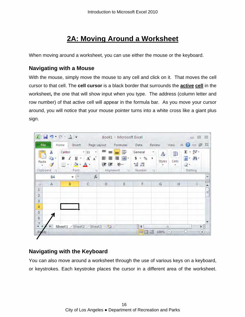
When moving around a worksheet, you can use either the mouse or the keyboard.

Navigating with a Mouse With the mouse, simply move the mouse to any cell and click on it. That moves the cell

cursor to that cell. The cell cursor is a black border that surrounds the active cell in the

worksheet, the one that will show input when you type. The address (column letter and

row number) of that active cell will appear in the formula bar. As you move your cursor

around, you will notice that your mouse pointer turns into a white cross like a giant plus

sign.

Navigating with the Keyboard You can also move around a worksheet through the use of various keys on a keyboard,

or keystrokes. Each keystroke places the cursor in a different area of the worksheet.



http://www.dummies.com/how-to/content/how-to-select-cells-in-excel-2010.html#glossary-active_cell

http://www.dummies.com/how-to/content/how-to-select-cells-in-excel-2010.html#glossary-active_cell

Keystroke Guide to Navigating Your Worksheet

The following is a guide to other keystrokes to move around the worksheet. Practice all

of these keystrokes on your worksheet.

Keystroke Where the Cell Cursor Moves

Right arrow or Tab Cell to the immediate right.

Left arrow or Shift + Tab Cell to the immediate left.

Up arrow Cell up one row.

Down arrow Cell down one row.

Home Cell in Column A of the current row.

Ctrl + Home First cell (A1) of the worksheet.

Ctrl + End or

End, Home

Cell in the worksheet at the intersection of the last column that has

data in it and the last row that has data in it (that is, the last cell of

the active area of the worksheet).

Page Up Cell one full screen up in the same column.

Page Down Cell one full screen down in the same column.

Ctrl + Right arrow or

End, Right arrow

First occupied cell to the right in the same row that is either

preceded or followed by a blank cell. If no cell is occupied, the

pointer goes to the cell at the very end of the row.

Ctrl + Left arrow or End,

Left arrow

First occupied cell to the left in the same row that is either preceded

or followed by a blank cell. If no cell is occupied, the pointer goes to

the cell at the very beginning of the row.

Ctrl + Up arrow or End,

Up arrow

First occupied cell above in the same column that is either preceded


the cell at the very top of the column.

Ctrl + Down arrow or

End, Down arrow

First occupied cell below in the same column that is either preceded


the cell at the very bottom of the column.

Ctrl + Page Down The cell pointer’s location in the next worksheet of that workbook.

Ctrl + Page Up The cell pointer’s location in the previous worksheet of that

workbook.



http://www.dummies.com/how-to/content/moving-the-cell-cursor-in-excel-2010-spreadsheets.navId-405650.html#glossary-tabs

http://www.dummies.com/how-to/content/moving-the-cell-cursor-in-excel-2010-spreadsheets.navId-405650.html#glossary-workbook

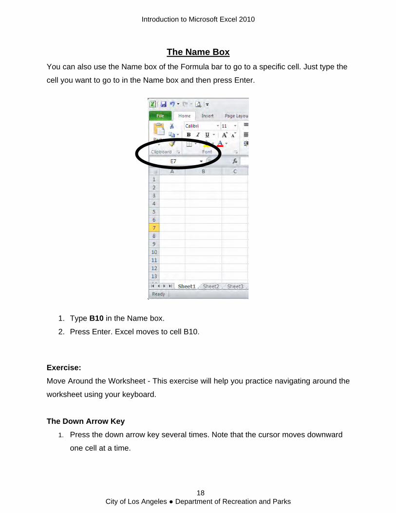
The Name Box You can also use the Name box of the Formula bar to go to a specific cell. Just type the

cell you want to go to in the Name box and then press Enter.

1. Type B10 in the Name box.

2. Press Enter. Excel moves to cell B10.

Exercise: Move Around the Worksheet - This exercise will help you practice navigating around the

worksheet using your keyboard.

The Down Arrow Key 1. Press the down arrow key several times. Note that the cursor moves downward

one cell at a time.




The Up Arrow Key

1. Press the up arrow key several times. Note that the cursor moves upward one

cell at a time.

The Tab Key

1. Move to cell A1 with your arrow keys.

2. Press the Tab key several times. Note that the cursor moves to the right one cell

at a time.

The Shift + Tab Keys 1. Hold down the Shift key and then press Tab. Note that the cursor moves to the

left one cell at a time.

The Right and Left Arrow Keys 1. Press the right arrow key several times. Note that the cursor moves to the right.

2. Press the left arrow key several times. Note that the cursor moves to the left.

Page Up and Page Down 1. Press the Page Down key. Note that the cursor moves down one page.

2. Press the Page Up key. Note that the cursor moves up one page.

The Ctrl + Home Key

1. Move the cursor to column J, row 1, using the arrow keys.

2. Stay in column J and move the cursor to row 20.

3. Hold down the Ctrl key while you press the Home key. Excel moves to cell A1.



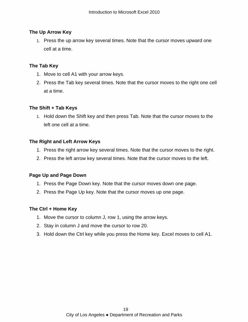
2B: Select Cells

If you wish to perform a function on a group of cells, you must first select those cells by

highlighting them. One way to select cells is by using your mouse.

Select Cells by Dragging You can select an area by holding down the left mouse button and move the mouse

over the area. This is called dragging.

Exercise: To select cells A1 to E7:

1. Go to cell A1.

2. Press the left mouse button on A1.

3. While holding down the left mouse button, move the mouse from A1 to E7.

4. Excel highlights cells A1 to E7.

5. Click anywhere on the worksheet to clear the highlighting.



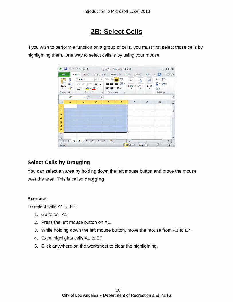
Selecting Multiple Cell Areas You can also multiple cell areas in different areas of the worksheet with the use of the

Ctrl button along with the mouse.

Exercise: Choosing Multiple Cell Areas

1. Go to cell A1.

2. Press the left mouse button on A1.

3. While holding down the left mouse button, use the mouse to move from cell A1 to

C5.

4. Hold down the Ctrl key, but release the left mouse button.

5. Using the mouse, place the cursor in cell D7.

6. Press the left mouse button. While holding down the left mouse button, move to

cell F10. Release the left mouse button.

7. Release the Ctrl key. Cells A1 to C5 and cells D7 to F10 are selected.

8. Click anywhere on the worksheet to remove the highlighting.



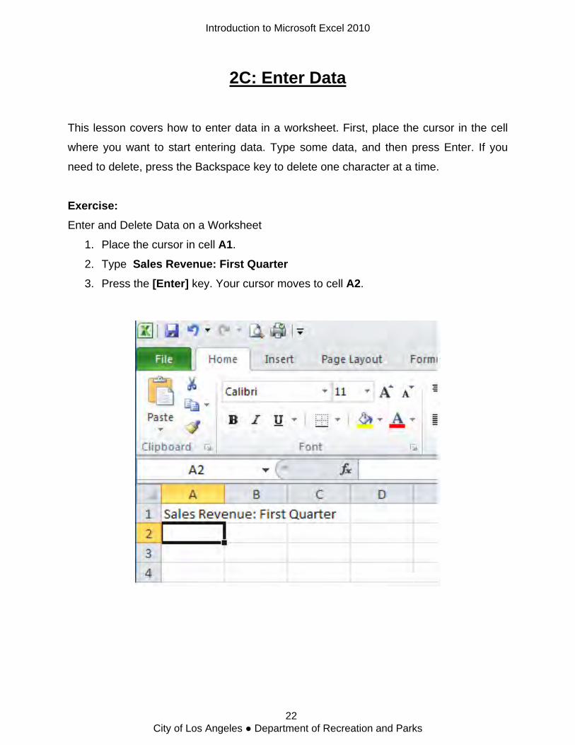
2C: Enter Data

This lesson covers how to enter data in a worksheet. First, place the cursor in the cell

where you want to start entering data. Type some data, and then press Enter. If you

need to delete, press the Backspace key to delete one character at a time.

Exercise: Enter and Delete Data on a Worksheet

1. Place the cursor in cell A1.

2. Type Sales Revenue: First Quarter 3. Press the [Enter] key. Your cursor moves to cell A2.



2D: Edit a Cell

After you enter data into a cell, you can edit the data by double clicking on the cell you

wish to edit.

Edit a Cell by Double-Clicking in the Cell 1. Use the up arrow key to move your cursor to cell A1.

2. Double-click in cell A1. You should see a blinking cursor inside the cell where

you double clicked.

3. Use the arrow keys to move the cursor in front of the word First. 4. Use the [Delete] key to erase First. 5. Type Second. 6. Press [Enter].

Exercise: Editing a Cell by Using the Formula Bar - An alternate method of editing a cell is using

the Formula bar.

1. Use the up arrow key to move your cursor to cell A1.

2. Click in the formula area of the Formula bar.

3. Use the arrow keys to move the cursor in front of the word Second.

4. Use the [Delete] key to erase Second.

5. Type Third.

6. Press [Enter]

Exercise: Change a Cell Entry - Typing a cell replaces the old cell entry with the new information

you type. This is known as Over-Typing.

1. Move the cursor to cell A1.

2. Type Sales Income: First Quarter. 3. Press [Enter]. The original data is replaced.



Exercise: Delete a Cell Entry - To delete an entry in a cell or a group of cells, you place the cursor

in the cell or select the group of cells and press Delete.

1. Select cell A1.

2. Press the [Delete] key. The name Sales Income: First Quarter is erased.

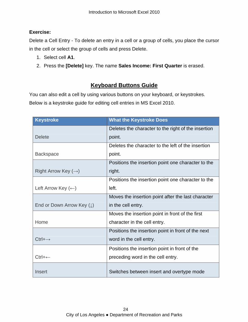
Keyboard Buttons Guide You can also edit a cell by using various buttons on your keyboard, or keystrokes.

Below is a keystroke guide for editing cell entries in MS Excel 2010.

Keystroke What the Keystroke Does

Delete

Deletes the character to the right of the insertion

point.

Backspace

Deletes the character to the left of the insertion

point.

Right Arrow Key (→)

Positions the insertion point one character to the

right.

Left Arrow Key (←)

Positions the insertion point one character to the

left.

End or Down Arrow Key (↓)

Moves the insertion point after the last character

in the cell entry.

Home

Moves the insertion point in front of the first

character in the cell entry.

Ctrl+→

Positions the insertion point in front of the next

word in the cell entry.

Ctrl+←

Positions the insertion point in front of the

preceding word in the cell entry.

Insert Switches between insert and overtype mode



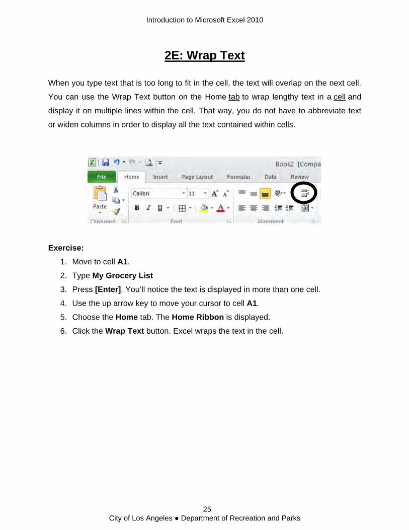
2E: Wrap Text

When you type text that is too long to fit in the cell, the text will overlap on the next cell.

You can use the Wrap Text button on the Home tab to wrap lengthy text in a cell and

display it on multiple lines within the cell. That way, you do not have to abbreviate text

or widen columns in order to display all the text contained within cells.

Exercise: 1. Move to cell A1.

2. Type My Grocery List 3. Press [Enter]. You’ll notice the text is displayed in more than one cell.

4. Use the up arrow key to move your cursor to cell A1.

5. Choose the Home tab. The Home Ribbon is displayed.

6. Click the Wrap Text button. Excel wraps the text in the cell.



http://www.dummies.com/how-to/content/how-to-wrap-excel-2010-data-to-see-all-the-text.html#glossary-tabs

http://www.dummies.com/how-to/content/how-to-wrap-excel-2010-data-to-see-all-the-text.html#glossary-cell

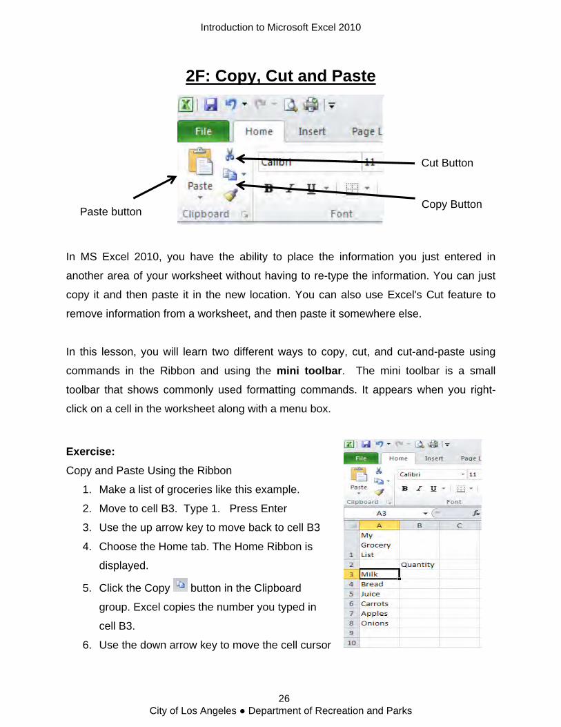
2F: Copy, Cut and Paste

Paste button

Copy Button

Cut Button

In MS Excel 2010, you have the ability to place the information you just entered in

another area of your worksheet without having to re-type the information. You can just

copy it and then paste it in the new location. You can also use Excel's Cut feature to

remove information from a worksheet, and then paste it somewhere else.

In this lesson, you will learn two different ways to copy, cut, and cut-and-paste using

commands in the Ribbon and using the mini toolbar. The mini toolbar is a small

toolbar that shows commonly used formatting commands. It appears when you right-

click on a cell in the worksheet along with a menu box.

Exercise: Copy and Paste Using the Ribbon

1. Make a list of groceries like this example.

2. Move to cell B3. Type 1. Press Enter

3. Use the up arrow key to move back to cell B3

4. Choose the Home tab. The Home Ribbon is

displayed.

5. Click the Copy button in the Clipboard

group. Excel copies the number you typed in

cell B3.

6. Use the down arrow key to move the cell cursor



in cell B4.

7. Click the Paste button in the Clipboard group. Excel pastes the data in cell

B3 into cell B4.

8. Use the down arrow key to move the cell cursor in cell B5.

9. Click the Paste button in the Clipboard group. Cell B5 will contain the same

data in cell B3.

10. Press the Esc key to exit the Copy mode.

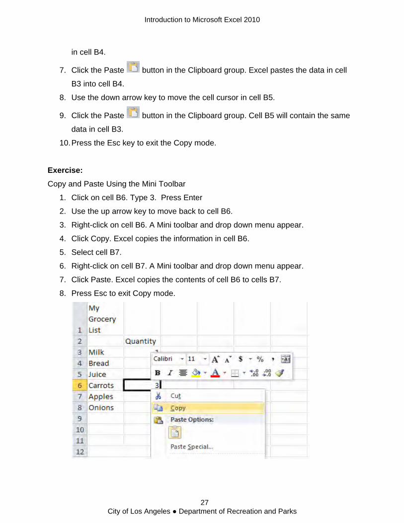
Exercise: Copy and Paste Using the Mini Toolbar

1. Click on cell B6. Type 3. Press Enter

2. Use the up arrow key to move back to cell B6.

3. Right-click on cell B6. A Mini toolbar and drop down menu appear.

4. Click Copy. Excel copies the information in cell B6.

5. Select cell B7.

6. Right-click on cell B7. A Mini toolbar and drop down menu appear.

7. Click Paste. Excel copies the contents of cell B6 to cells B7.

8. Press Esc to exit Copy mode.



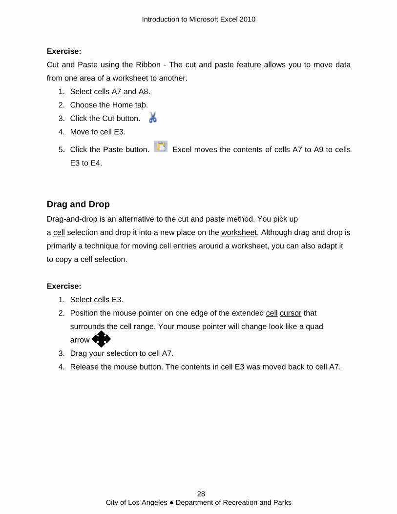
Exercise: Cut and Paste using the Ribbon - The cut and paste feature allows you to move data

from one area of a worksheet to another.

1. Select cells A7 and A8.

2. Choose the Home tab.

3. Click the Cut button.

4. Move to cell E3.

5. Click the Paste button. Excel moves the contents of cells A7 to A9 to cells

E3 to E4.

Drag and Drop Drag-and-drop is an alternative to the cut and paste method. You pick up

a cell selection and drop it into a new place on the worksheet. Although drag and drop is

primarily a technique for moving cell entries around a worksheet, you can also adapt it

to copy a cell selection.

Exercise: 1. Select cells E3.

2. Position the mouse pointer on one edge of the extended cell cursor that

surrounds the cell range. Your mouse pointer will change look like a quad

arrow

3. Drag your selection to cell A7.

4. Release the mouse button. The contents in cell E3 was moved back to cell A7.



http://www.dummies.com/how-to/content/how-to-drag-and-drop-data-in-excel-2010.html#glossary-cell

http://www.dummies.com/how-to/content/how-to-drag-and-drop-data-in-excel-2010.html#glossary-worksheet

http://www.dummies.com/how-to/content/how-to-drag-and-drop-data-in-excel-2010.html#glossary-cell_cursor

http://www.dummies.com/how-to/content/how-to-drag-and-drop-data-in-excel-2010.html#glossary-cell_cursor

2G: Columns and Rows

You can insert and delete columns and rows. When you delete a column, you delete

everything in the column from the top of the worksheet to the bottom of the worksheet.

When you delete a row, you delete the entire row from left to right. Inserting a column or

row inserts a completely new column or row.

Exercise: Delete and Insert Columns and Rows

2

1

3

To delete column E: 1. Click on column E. Column E will be highlighted

2. Choose the Home tab. Click the down arrow next to Delete in the Cells group. A

menu appears.

3. Click Delete Sheet Columns. The column you selected will be deleted.

4. Click anywhere on the worksheet to remove your selection.



To delete row 8: 1. Click on row 8. Row 8 will be highlighted.

2. In the Home Ribbon, click the down arrow next to Delete in the Cells group. A

menu appears.

3. Click Delete Sheet Rows. The row you selected will be deleted.

4. Click anywhere on the worksheet to remove your selection.

To insert a column:

1. Click on column B. The whole column will be highlighted

2. Click the down arrow next to Insert in the Cells group. A menu appears.

3. Click Insert Sheet Columns. A new column will be inserted to the left.

To insert a row:

1. Click on row 5 and drag the cursor down to 7 . Rows 5-7 will be highlighted.

2. Click the down arrow next to Insert in the Cells group. A menu appears.

3. Click Insert Sheet Rows. New rows will be inserted above the data.



2H: New Worksheet

In Microsoft Excel, each workbook is made up of several worksheets. Each worksheet

has a tab. By default, a workbook has three sheets and they are named sequentially,

starting with Sheet1. The name of the worksheet appears on the tab. Before moving to

the next topic, move to a new worksheet. The exercise that follows shows you how.

Exercise: Move to a New Worksheet

1. Click Sheet2 in the lower-left corner of the screen. Excel moves to Sheet2.



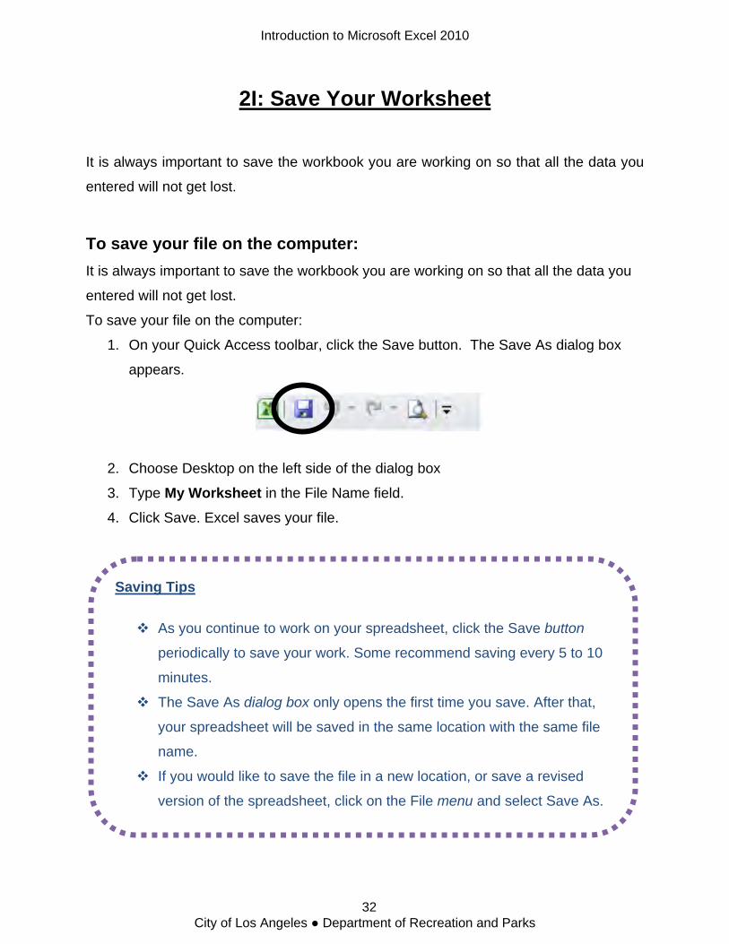
2I: Save Your Worksheet

It is always important to save the workbook you are working on so that all the data you

entered will not get lost.

To save your file on the computer: It is always important to save the workbook you are working on so that all the data you

entered will not get lost.

To save your file on the computer:

1. On your Quick Access toolbar, click the Save button. The Save As dialog box

appears.

2. Choose Desktop on the left side of the dialog box

3. Type My Worksheet in the File Name field.

4. Click Save. Excel saves your file.

Saving Tips

As you continue to work on your spreadsheet, click the Save button

periodically to save your work. Some recommend saving every 5 to 10

minutes.

The Save As dialog box only opens the first time you save. After that,

your spreadsheet will be saved in the same location with the same file

name.

If you would like to save the file in a new location, or save a revised

version of the spreadsheet, click on the File menu and select Save As.



2J: Close, Open and Exit

In this lesson, you will learn how to close the workbook, open it again, and exit MS

Excel 2010.

Closing Your Workbook This will only close the existing workbook, not exit out of MS Excel entirely. If you have

already saved your work, you can close your workbook by doing the following:

1. Go to the File Ribbon

2. Select “Close”

Opening a Workbook 1. Go the File Ribbon

2. Select “Open”

3. Select the workbook you wish to open.

• To open the workbook you saved on the computer, choose “Desktop” on

the left side of the dialog box, and choose “My Worksheet” in the dialog

box.

4. Click “Open”

Exiting MS Excel To exit Excel, you have two options:

1. Go to the File Ribbon and click on “Exit.”

2. Click on the ‘X’ button in upper right corner of the Title bar.



Lesson 3: Basic Formats and

Formulas



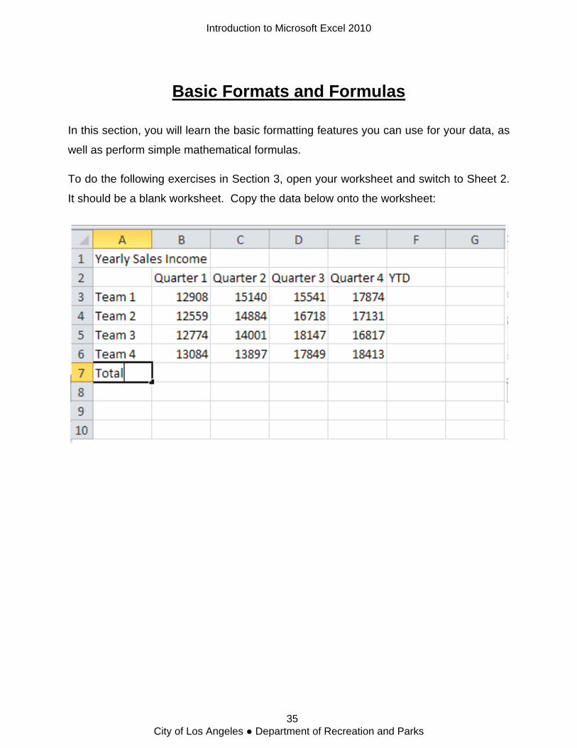
Basic Formats and Formulas

In this section, you will learn the basic formatting features you can use for your data, as

well as perform simple mathematical formulas.

To do the following exercises in Section 3, open your worksheet and switch to Sheet 2.

It should be a blank worksheet. Copy the data below onto the worksheet:



3A: Borders

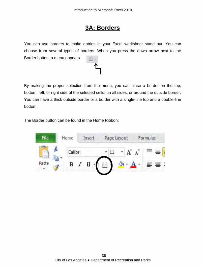
You can use borders to make entries in your Excel worksheet stand out. You can

choose from several types of borders. When you press the down arrow next to the

Border button, a menu appears.

By making the proper selection from the menu, you can place a border on the top,

bottom, left, or right side of the selected cells; on all sides; or around the outside border.

You can have a thick outside border or a border with a single-line top and a double-line

bottom.

The Border button can be found in the Home Ribbon:



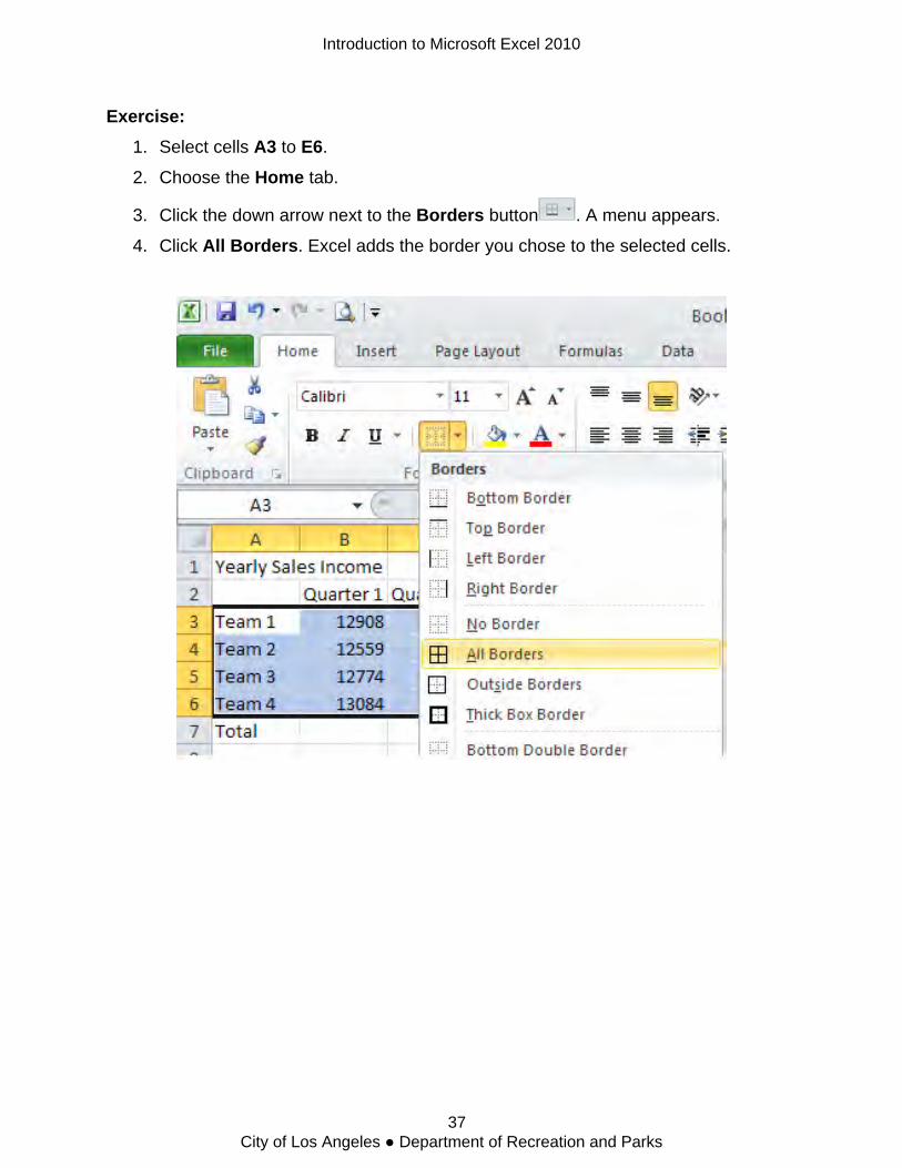
Exercise: 1. Select cells A3 to E6.


3. Click the down arrow next to the Borders button . A menu appears.

4. Click All Borders. Excel adds the border you chose to the selected cells.



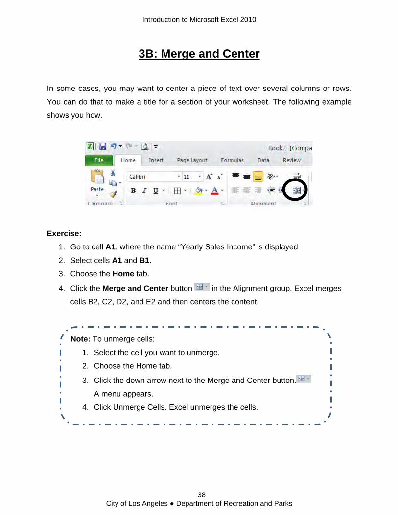
3B: Merge and Center

In some cases, you may want to center a piece of text over several columns or rows.

You can do that to make a title for a section of your worksheet. The following example

shows you how.

Exercise: 1. Go to cell A1, where the name “Yearly Sales Income” is displayed

2. Select cells A1 and B1.


4. Click the Merge and Center button in the Alignment group. Excel merges

cells B2, C2, D2, and E2 and then centers the content.


3. Click the down arrow next to the Merge and Center button.

A menu appears.

4. Click Unmerge Cells. Excel unmerges the cells.

1. Select the cell you want to unmerge.

Note: To unmerge cells:



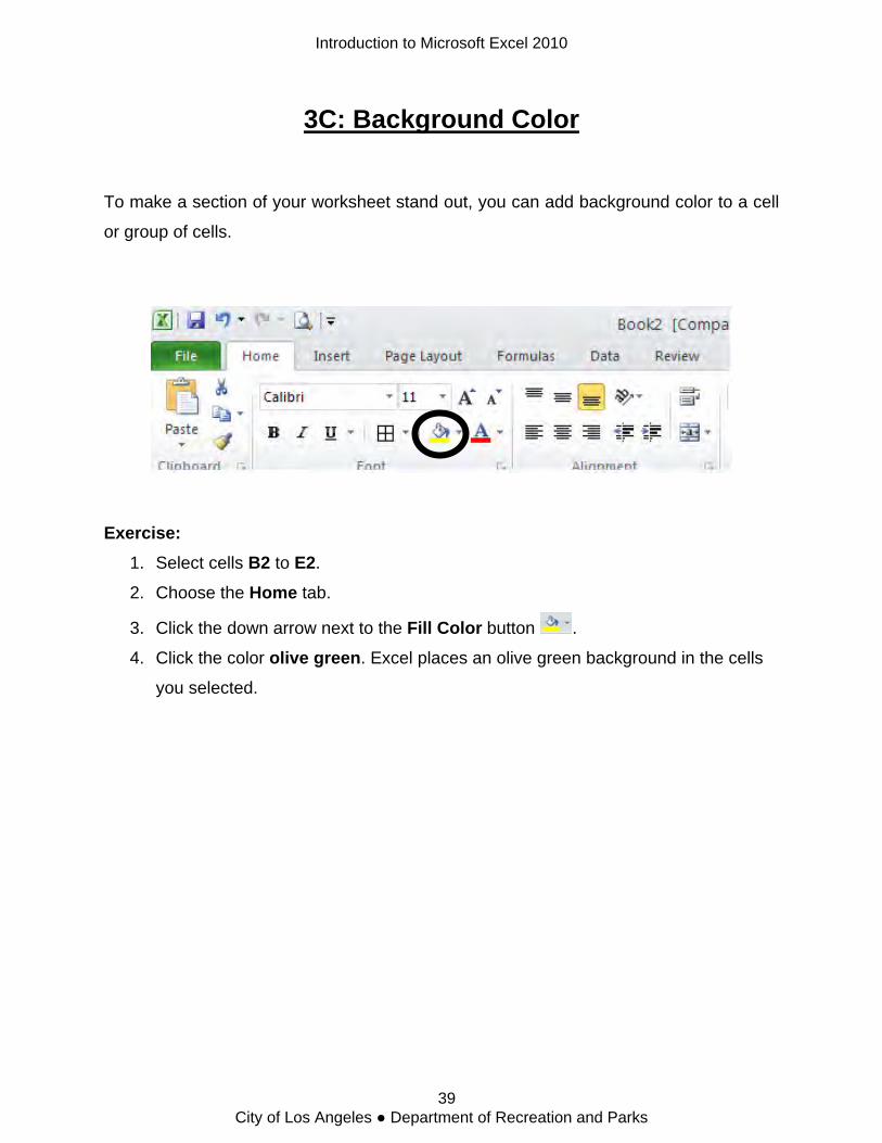
3C: Background Color

To make a section of your worksheet stand out, you can add background color to a cell

or group of cells.

Exercise: 1. Select cells B2 to E2.


3. Click the down arrow next to the Fill Color button .

4. Click the color olive green. Excel places an olive green background in the cells

you selected.



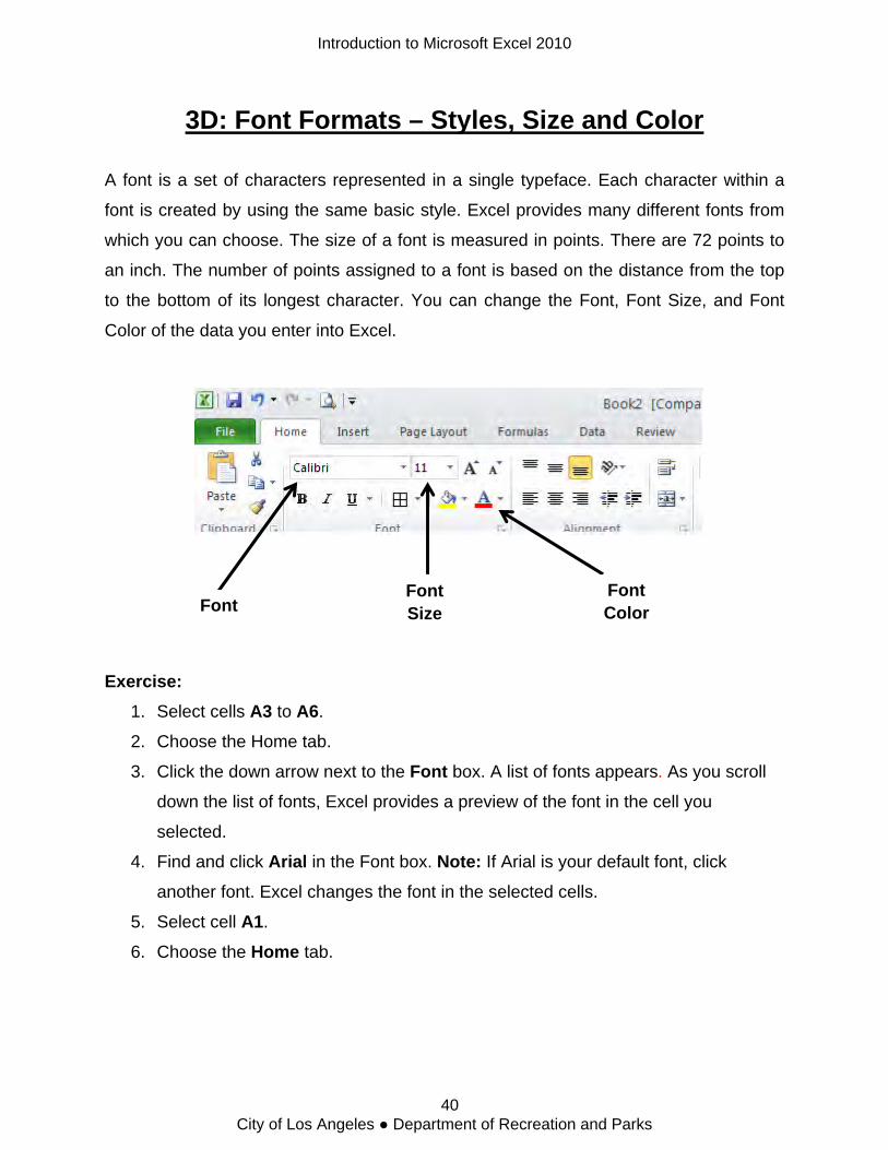
3D: Font Formats – Styles, Size and Color

A font is a set of characters represented in a single typeface. Each character within a

font is created by using the same basic style. Excel provides many different fonts from

which you can choose. The size of a font is measured in points. There are 72 points to

an inch. The number of points assigned to a font is based on the distance from the top

to the bottom of its longest character. You can change the Font, Font Size, and Font

Color of the data you enter into Excel.

Font Color Font

Font Size

Exercise:

1. Select cells A3 to A6.


3. Click the down arrow next to the Font box. A list of fonts appears. As you scroll

down the list of fonts, Excel provides a preview of the font in the cell you

selected.

4. Find and click Arial in the Font box. Note: If Arial is your default font, click

another font. Excel changes the font in the selected cells.

5. Select cell A1.




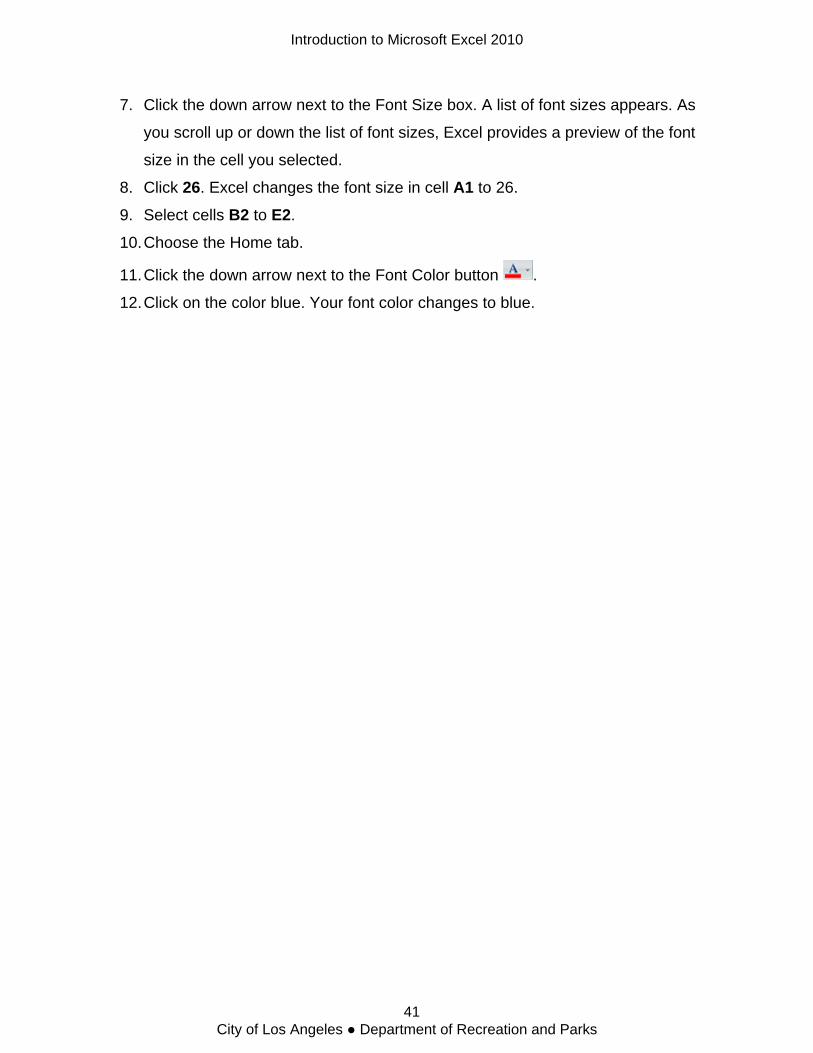
7. Click the down arrow next to the Font Size box. A list of font sizes appears. As

you scroll up or down the list of font sizes, Excel provides a preview of the font

size in the cell you selected.

8. Click 26. Excel changes the font size in cell A1 to 26.

9. Select cells B2 to E2.


11. Click the down arrow next to the Font Color button .

12. Click on the color blue. Your font color changes to blue.



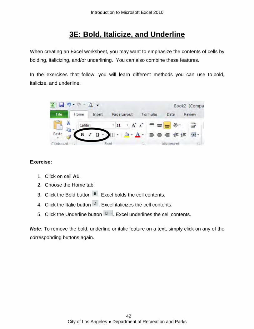
3E: Bold, Italicize, and Underline

When creating an Excel worksheet, you may want to emphasize the contents of cells by

bolding, italicizing, and/or underlining. You can also combine these features.

In the exercises that follow, you will learn different methods you can use to bold,

italicize, and underline.

Exercise:

1. Click on cell A1.


3. Click the Bold button . Excel bolds the cell contents.

4. Click the Italic button . Excel italicizes the cell contents.

5. Click the Underline button . Excel underlines the cell contents.

Note: To remove the bold, underline or italic feature on a text, simply click on any of the

corresponding buttons again.



3F: Text Alignment When you type text into a cell, by default your entry aligns with the left side of the cell.

When you type numbers into a cell, by default your entry aligns with the right side of the

cell. You can change the cell alignment. You can center, left-align, or right-align any cell

entry. Look at cells A1 to D1. Note that they are aligned with the left side of the cell.

Exercise: Center-Align - To center cells A2 to F7:

1. Select cells A2 to F7.


3. Click the Center button in the Alignment group. Excel centers each cell's

content.

Left-Align - To left-align cells A2 to F7: 1. Select cells A2 to F7.


3. Click the Align Text Left button in the Alignment group. Excel left-aligns

each cell's content.

Right-Align - To right-align cells A2 to F7:

1. Select cells A2 to F7.


3. Click the Align Text Right button. Excel right-aligns the cell's content.

4. Click anywhere on your worksheet to clear the highlighting.



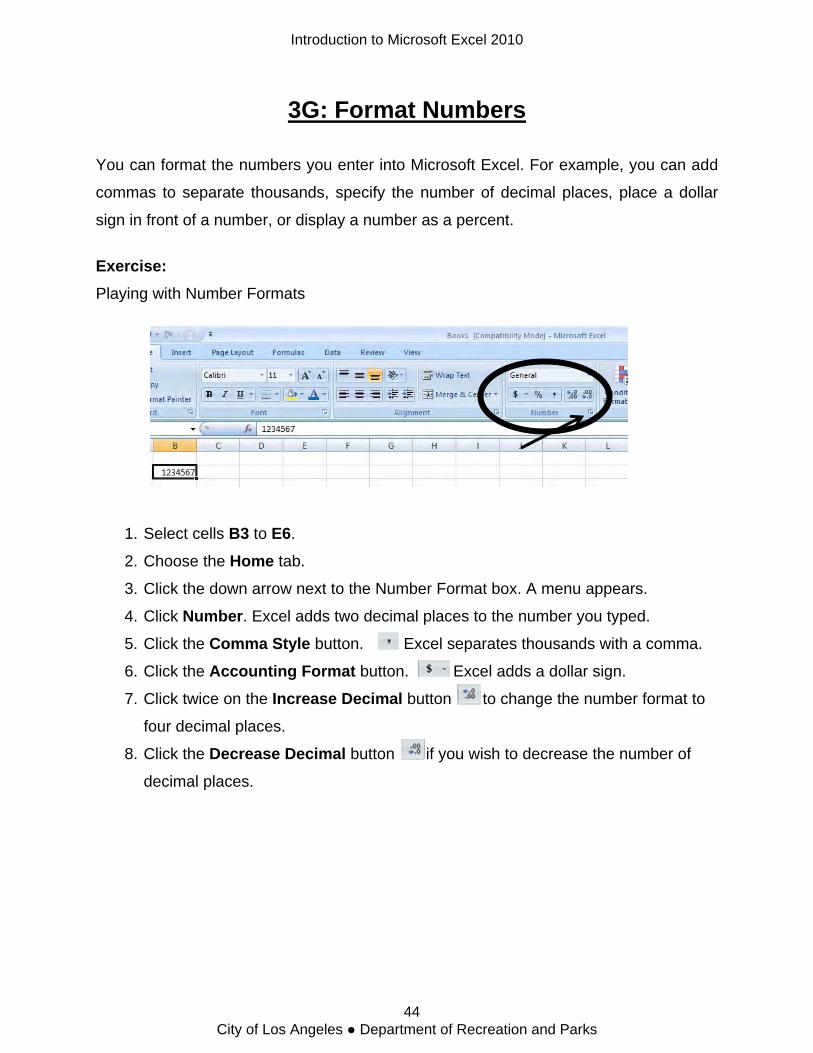
3G: Format Numbers

You can format the numbers you enter into Microsoft Excel. For example, you can add

commas to separate thousands, specify the number of decimal places, place a dollar

sign in front of a number, or display a number as a percent.

Exercise: Playing with Number Formats

1. Select cells B3 to E6.


3. Click the down arrow next to the Number Format box. A menu appears.

4. Click Number. Excel adds two decimal places to the number you typed.

5. Click the Comma Style button. Excel separates thousands with a comma.

6. Click the Accounting Format button. Excel adds a dollar sign.

7. Click twice on the Increase Decimal button to change the number format to

four decimal places.

8. Click the Decrease Decimal button if you wish to decrease the number of

decimal places.



Change a Decimal to a Percent. 1. Move to cell B10.

2. Type .35 (note the decimal point).

3. Click the check mark on the formula bar.


5. Click the Percent Style button . Excel turns the decimal into a percent.



3H: Perform Mathematical Calculations

A major strength of MS Excel 2010 is that you can perform mathematical calculations

with your data and format the results. In this lesson, you learn how to perform basic

mathematical calculations and how to format text and numerical data.

Formulas in Excel must have 3 parts: equal sign (=), one or more cell references

(addresses, ex. A1), and the operator sign for the type of calculation you want to do to

on the data (add, subtract, multiply, divide). Use the following to indicate the type of

calculation you wish to perform:

+ Addition

- Subtraction

* Multiplication

/ Division

^ Exponential

Exercise: Basic Math on Excel - In this exercise, you will practice some of the methods you can

use to move around a worksheet and you learn how to perform mathematical

calculations. Switch to Sheet 3 and type information as show in the Example into your

blank worksheet.



1. Double click on A4 to place cursor in cell, and do the following:

a. Press the equal sign (=) button

b. Click on Cell A2

c. Press the plus (+) button

d. Click on cell A3

e. Press Enter

2. The result will display in A4

3. You will do the same for columns B, C, and D but for part C of the instructions

you will be doing a different calculation for each row:

• Column B – press the minus (-) button

• Column C – press the asterisk (*) button

• Column D – press the forward slash (/) button



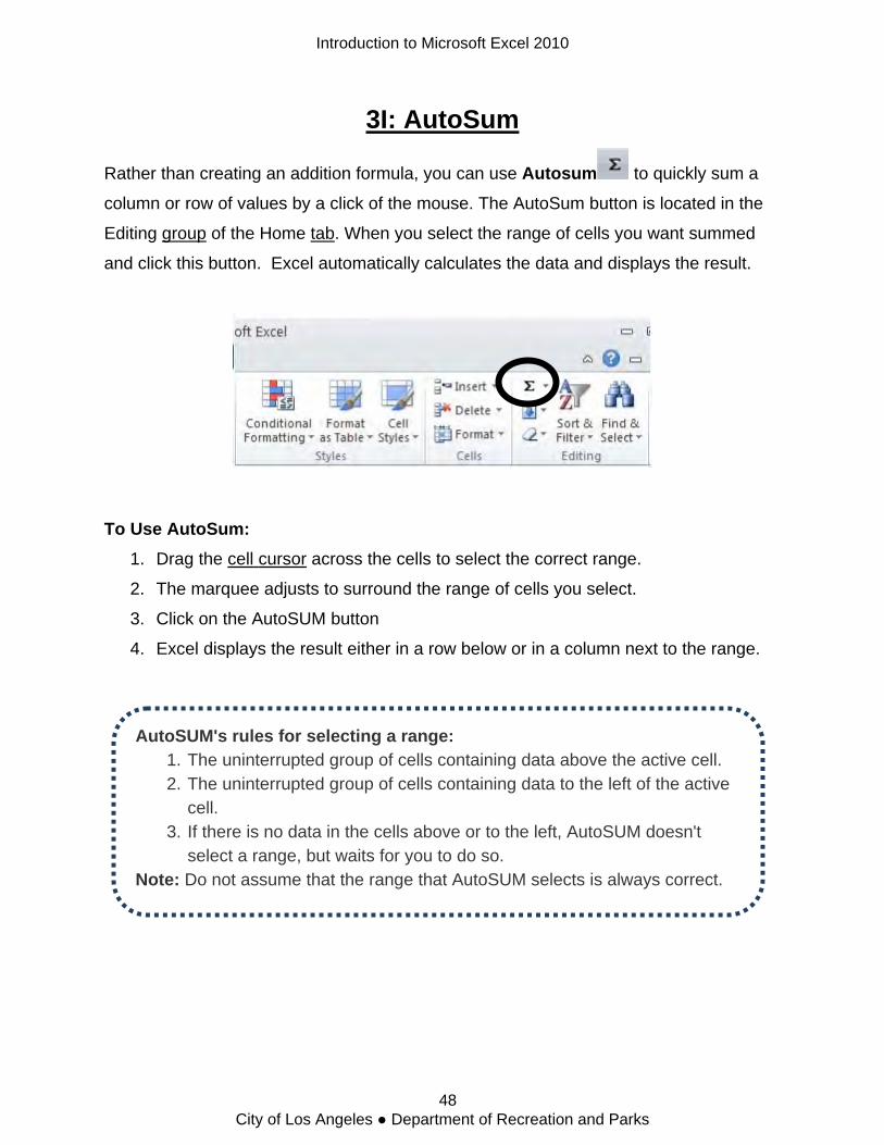
3I: AutoSum

Rather than creating an addition formula, you can use Autosum to quickly sum a

column or row of values by a click of the mouse. The AutoSum button is located in the

Editing group of the Home tab. When you select the range of cells you want summed

and click this button. Excel automatically calculates the data and displays the result.

To Use AutoSum: 1. Drag the cell cursor across the cells to select the correct range.

2. The marquee adjusts to surround the range of cells you select.

3. Click on the AutoSUM button

4. Excel displays the result either in a row below or in a column next to the range.

AutoSUM's rules for selecting a range: 1. The uninterrupted group of cells containing data above the active cell. 2. The uninterrupted group of cells containing data to the left of the active

cell. 3. If there is no data in the cells above or to the left, AutoSUM doesn't

select a range, but waits for you to do so. Note: Do not assume that the range that AutoSUM selects is always correct.



http://www.dummies.com/how-to/content/using-autosum-for-quick-calculations-in-excel-2010.html#glossary-group

http://www.dummies.com/how-to/content/using-autosum-for-quick-calculations-in-excel-2010.html#glossary-tabs

http://www.dummies.com/how-to/content/using-autosum-for-quick-calculations-in-excel-2010.html#glossary-cell_cursor

http://www.dummies.com/how-to/content/using-autosum-for-quick-calculations-in-excel-2010.html#glossary-cell_cursor

Exercise: For the following exercise, you will use the data entered in sheet 2.

1. Select cells B3 through B6.


3. Click the AutoSum button in the Editing group. Excel will display the result in

cell B7.

4. Select cells B3 through E3


6. Click the AutoSum button in the Editing group. Excel will display the result in

cell F3.

Now perform AutoSUM for column C, D and E, as well as the AutoSUM totals for

rows 4, 5 and 6.



Lesson 4: Creating a Chart



Lesson 4A: Create a Chart This section will show you how to create a chart with the data you entered on your worksheet.

In MS Excel 2010, you can represent numbers in a chart. On the Insert tab, you can

choose from a variety of chart types, including column, line, pie, bar, area, and scatter.

The basic procedure for creating a chart is the same no matter what type of chart you

choose. As you change your data, your chart will automatically update.

You select a chart type by choosing an option from the Insert tab's Chart group. After

you choose a chart type, you will see a sub-menu with additional style choices. For

example, if you select Column Chart, you can choose to have your chart represented as

a two-dimensional chart, a three-dimensional chart, a cylinder chart, a cone chart, or a

pyramid chart. As you roll your mouse pointer over each option, Excel supplies a brief

description of each chart sub-type.

After you have created a worksheet data, you are ready to create your chart. For the

following exercises, we will use the data you entered in worksheet 2.



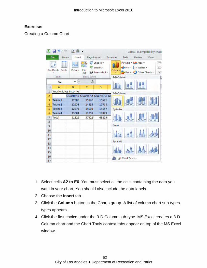
Exercise: Creating a Column Chart

1. Select cells A2 to E6. You must select all the cells containing the data you

want in your chart. You should also include the data labels.

2. Choose the Insert tab.

3. Click the Column button in the Charts group. A list of column chart sub-types

types appears.

4. Click the first choice under the 3-D Column sub-type. MS Excel creates a 3-D

Column chart and the Chart Tools context tabs appear on top of the MS Excel

window.



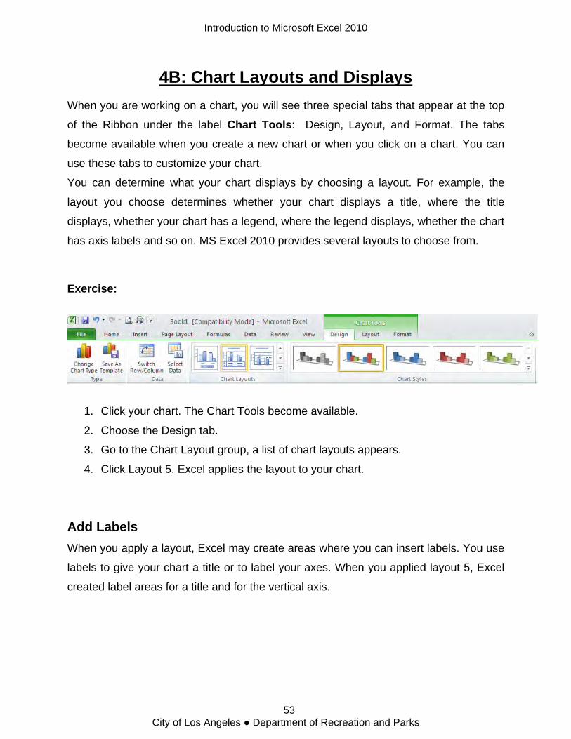
4B: Chart Layouts and Displays When you are working on a chart, you will see three special tabs that appear at the top

of the Ribbon under the label Chart Tools: Design, Layout, and Format. The tabs

become available when you create a new chart or when you click on a chart. You can

use these tabs to customize your chart.

You can determine what your chart displays by choosing a layout. For example, the

layout you choose determines whether your chart displays a title, where the title

displays, whether your chart has a legend, where the legend displays, whether the chart

has axis labels and so on. MS Excel 2010 provides several layouts to choose from.

Exercise:

1. Click your chart. The Chart Tools become available.

2. Choose the Design tab.

3. Go to the Chart Layout group, a list of chart layouts appears.

4. Click Layout 5. Excel applies the layout to your chart.

Add Labels When you apply a layout, Excel may create areas where you can insert labels. You use

labels to give your chart a title or to label your axes. When you applied layout 5, Excel

created label areas for a title and for the vertical axis.



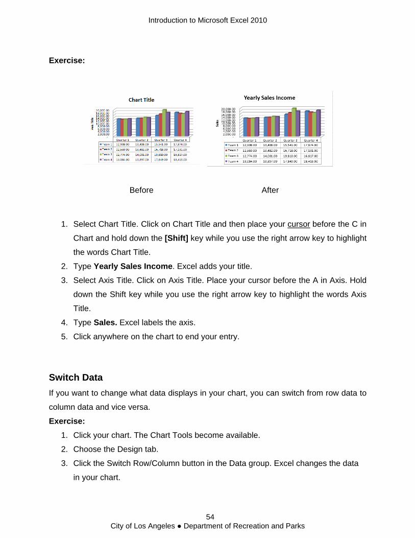
Exercise:

Before After

1. Select Chart Title. Click on Chart Title and then place your cursor before the C in

Chart and hold down the [Shift] key while you use the right arrow key to highlight

the words Chart Title.

2. Type Yearly Sales Income. Excel adds your title.

3. Select Axis Title. Click on Axis Title. Place your cursor before the A in Axis. Hold

down the Shift key while you use the right arrow key to highlight the words Axis

Title.

4. Type Sales. Excel labels the axis.

5. Click anywhere on the chart to end your entry.

Switch Data If you want to change what data displays in your chart, you can switch from row data to

column data and vice versa.

Exercise: 1. Click your chart. The Chart Tools become available.


3. Click the Switch Row/Column button in the Data group. Excel changes the data

in your chart.





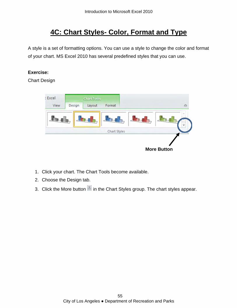
4C: Chart Styles- Color, Format and Type

A style is a set of formatting options. You can use a style to change the color and format

of your chart. MS Excel 2010 has several predefined styles that you can use.

Exercise: Chart Design

More Button



3. Click the More button in the Chart Styles group. The chart styles appear.



4. Click Style 42. Excel applies the style to your chart.

Chart Size and Position When you click a chart, handles appear on the right and left sides, the top and bottom,

and the corners of the chart. You can drag the handles on the top and bottom of the

chart to increase or decrease the height of the chart. You can drag the handles on the

left and right sides to increase or decrease the width of the chart. You can drag the

handles on the corners to increase or decrease the size of the chart proportionally. You

can change the position of a chart by clicking on an unused area of the chart and

dragging.

1. Use the handles to adjust the size of your chart.

2. Click an unused portion of the chart and drag to position the chart beside the

data.



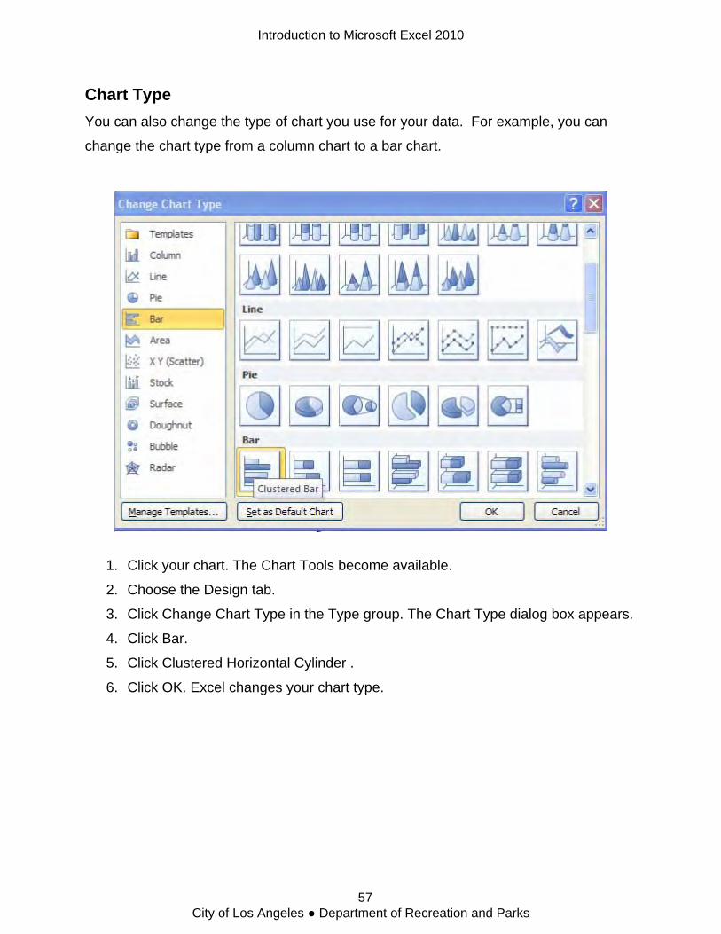
Chart Type You can also change the type of chart you use for your data. For example, you can

change the chart type from a column chart to a bar chart.



3. Click Change Chart Type in the Type group. The Chart Type dialog box appears.

4. Click Bar.

5. Click Clustered Horizontal Cylinder .

6. Click OK. Excel changes your chart type.



Lesson 5: Preview and Print

Your Work



5A: Page Layout

Print options are located on the Page Layout tab. You can also set your margins, set

your page orientation, and select your paper size.

Margins define the amount of white space that appears on the top, bottom, left, and

right edges of your document. The Margin option on the Page Layout tab provides

several standard margin sizes from which you can choose.

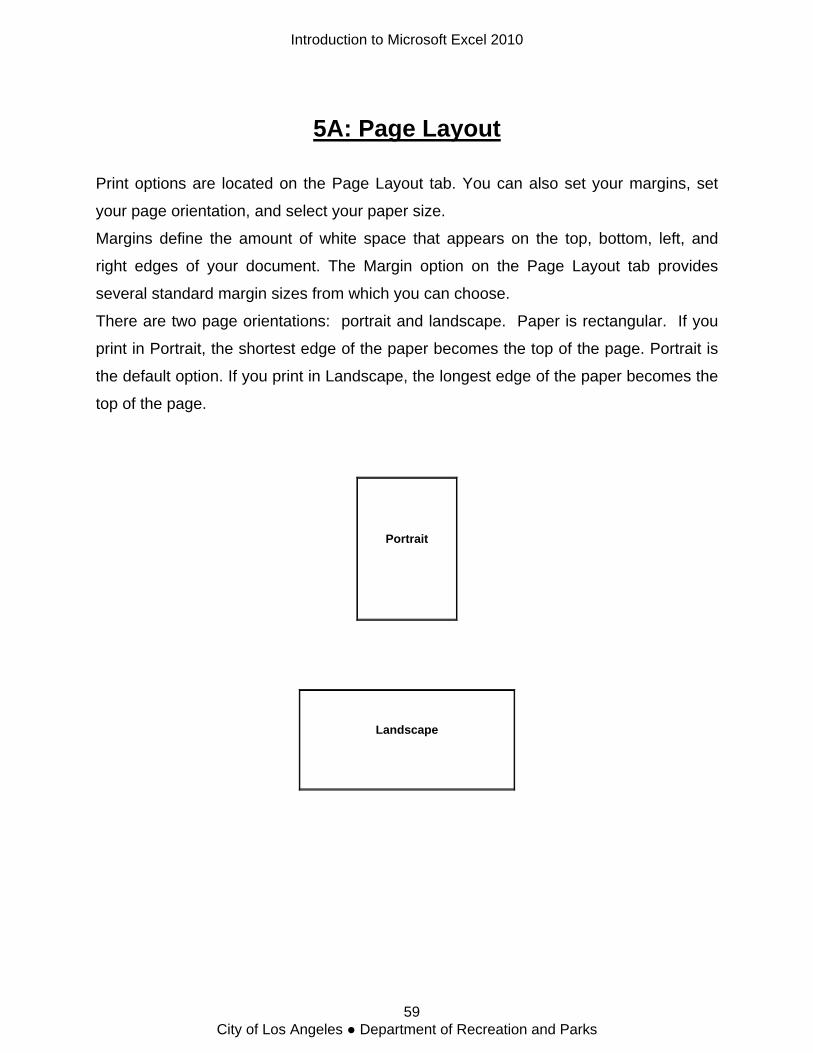
There are two page orientations: portrait and landscape. Paper is rectangular. If you

print in Portrait, the shortest edge of the paper becomes the top of the page. Portrait is

the default option. If you print in Landscape, the longest edge of the paper becomes the

top of the page.

Portrait

Landscape



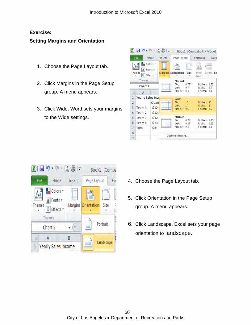
Exercise: Setting Margins and Orientation

1. Choose the Page Layout tab.

2. Click Margins in the Page Setup

group. A menu appears.

3. Click Wide. Word sets your margins

to the Wide settings.

4. Choose the Page Layout tab.

5. Click Orientation in the Page Setup

group. A menu appears.

6. Click Landscape. Excel sets your page

orientation to landscape.



5B: Print Preview and Print

The Print Preview and Print options can be found in the backstage view of MS Excel.

Prior to printing out your work, it is also a good idea to preview your material first. When

using Print Preview, you can see onscreen how your printed document will look when

you print it. If you click the Page Setup button while in Print Preview mode, you can set

page settings such as centering your data on the page or changing the margin areas.

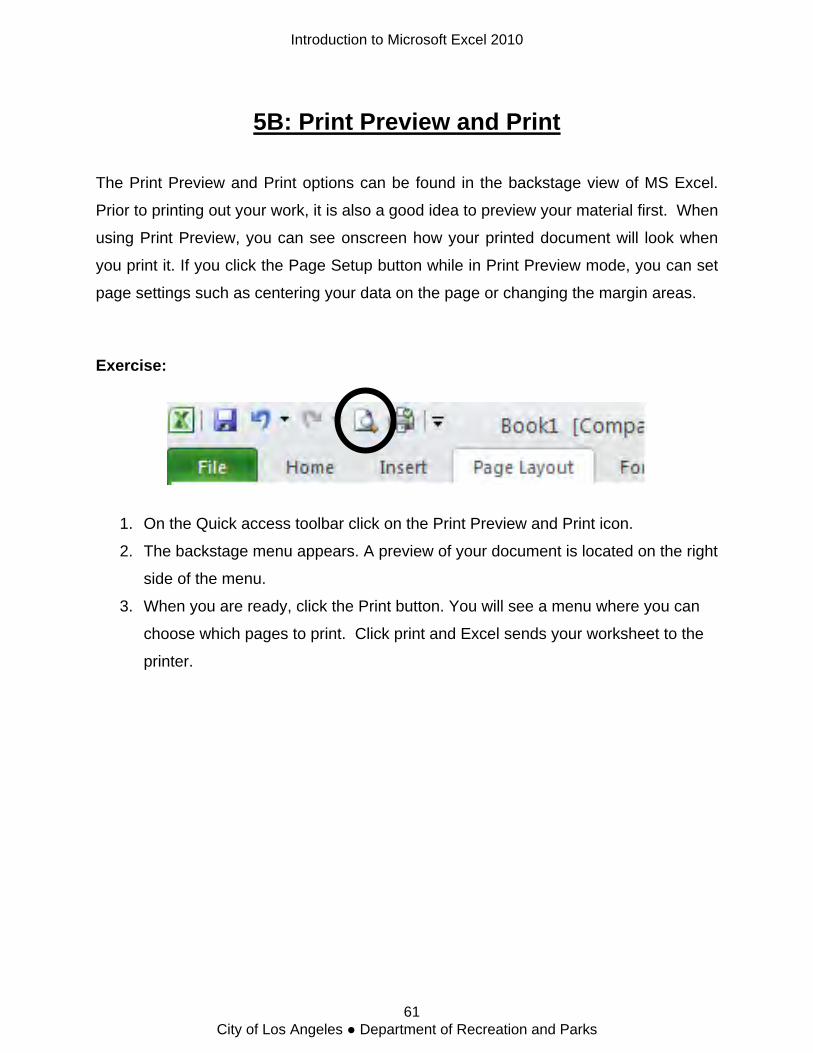
Exercise:

1. On the Quick access toolbar click on the Print Preview and Print icon.

2. The backstage menu appears. A preview of your document is located on the right

side of the menu.

3. When you are ready, click the Print button. You will see a menu where you can

choose which pages to print. Click print and Excel sends your worksheet to the

printer.



5C: Getting Help

This section will show you how to get help with MS Excel 2010.

The Help Dialog Box

1. Click on the Help icon on the far right side of the Ribbon.

2. Type: Backstage View in the top search bar

3. Read the topic “What and where is backstage view?”

4. Close the “Help Dialog Box”



Quick Reference Guide



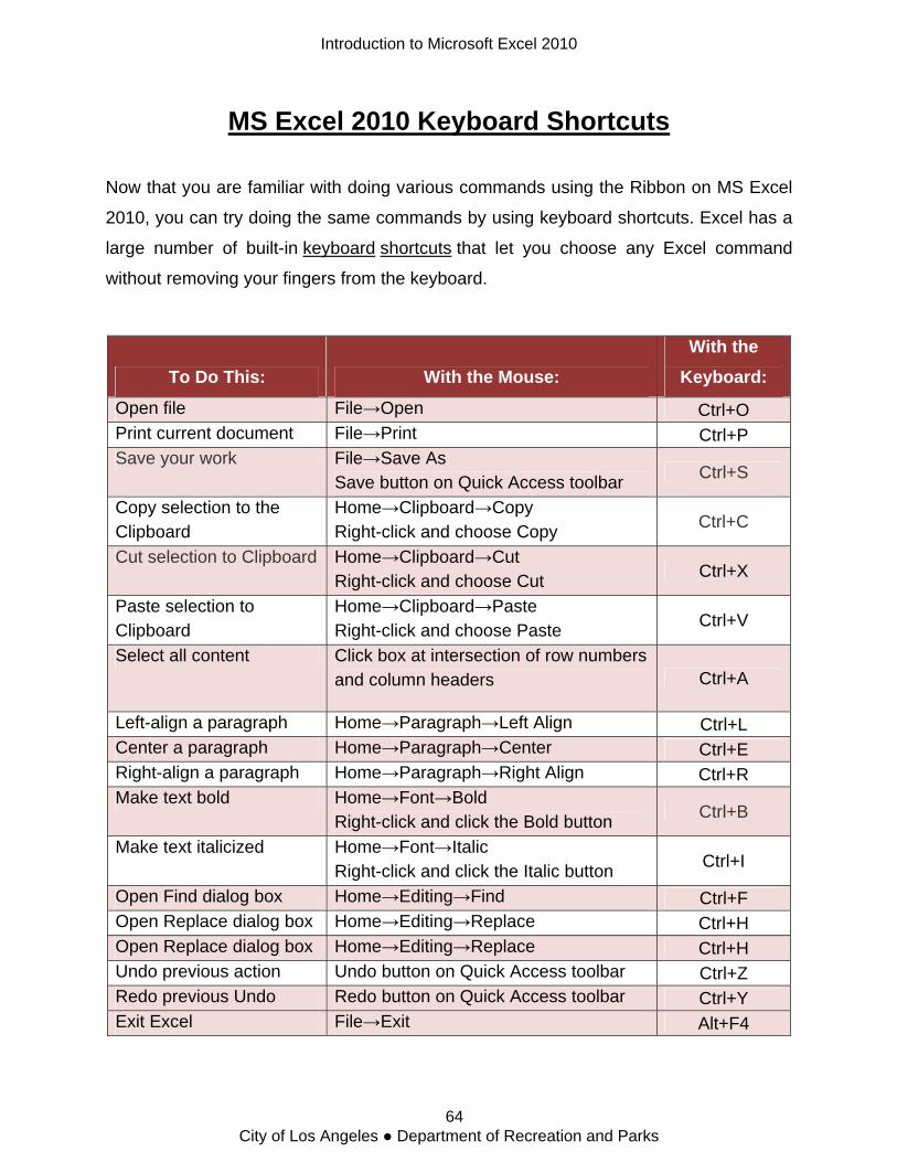
MS Excel 2010 Keyboard Shortcuts

Now that you are familiar with doing various commands using the Ribbon on MS Excel

2010, you can try doing the same commands by using keyboard shortcuts. Excel has a

large number of built-in keyboard shortcuts that let you choose any Excel command

without removing your fingers from the keyboard.

To Do This: With the Mouse: With the

Keyboard:

Open file File→Open Ctrl+O Print current document File→Print Ctrl+P Save your work File→Save As

Save button on Quick Access toolbar Ctrl+S

Copy selection to the Clipboard

Home→Clipboard→Copy Right-click and choose Copy Ctrl+C

Cut selection to Clipboard Home→Clipboard→Cut Right-click and choose Cut Ctrl+X

Paste selection to Clipboard

Home→Clipboard→Paste Right-click and choose Paste Ctrl+V

Select all content Click box at intersection of row numbers and column headers Ctrl+A

Left-align a paragraph Home→Paragraph→Left Align Ctrl+L Center a paragraph Home→Paragraph→Center Ctrl+E Right-align a paragraph Home→Paragraph→Right Align Ctrl+R Make text bold Home→Font→Bold

Right-click and click the Bold button Ctrl+B

Make text italicized Home→Font→Italic Right-click and click the Italic button Ctrl+I

Open Find dialog box Home→Editing→Find Ctrl+F Open Replace dialog box Home→Editing→Replace Ctrl+H Open Replace dialog box Home→Editing→Replace Ctrl+H Undo previous action Undo button on Quick Access toolbar Ctrl+Z Redo previous Undo Redo button on Quick Access toolbar Ctrl+Y Exit Excel File→Exit Alt+F4



http://www.dummies.com/how-to/content/how-to-select-excel-2010-commands-with-keyboard-sh.html#glossary-keyboard_shortcuts

http://www.dummies.com/how-to/content/how-to-select-excel-2010-commands-with-keyboard-sh.html#glossary-keyboard_shortcuts

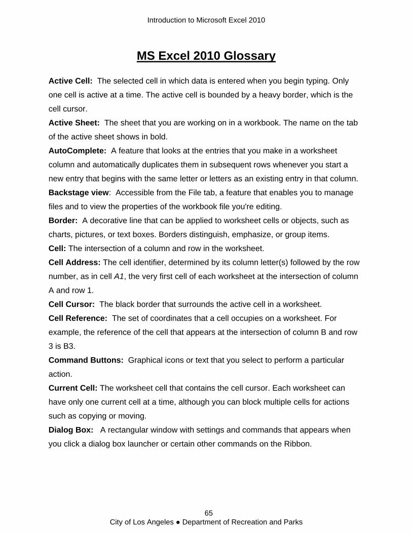
MS Excel 2010 Glossary

Active Cell: The selected cell in which data is entered when you begin typing. Only

one cell is active at a time. The active cell is bounded by a heavy border, which is the

cell cursor. Active Sheet: The sheet that you are working on in a workbook. The name on the tab

of the active sheet shows in bold. AutoComplete: A feature that looks at the entries that you make in a worksheet

column and automatically duplicates them in subsequent rows whenever you start a

new entry that begins with the same letter or letters as an existing entry in that column.

Backstage view: Accessible from the File tab, a feature that enables you to manage

files and to view the properties of the workbook file you're editing.

Border: A decorative line that can be applied to worksheet cells or objects, such as

charts, pictures, or text boxes. Borders distinguish, emphasize, or group items. Cell: The intersection of a column and row in the worksheet.

Cell Address: The cell identifier, determined by its column letter(s) followed by the row

number, as in cell A1, the very first cell of each worksheet at the intersection of column

A and row 1.

Cell Cursor: The black border that surrounds the active cell in a worksheet.

Cell Reference: The set of coordinates that a cell occupies on a worksheet. For

example, the reference of the cell that appears at the intersection of column B and row

3 is B3. Command Buttons: Graphical icons or text that you select to perform a particular

action.

Current Cell: The worksheet cell that contains the cell cursor. Each worksheet can

have only one current cell at a time, although you can block multiple cells for actions

such as copying or moving.

Dialog Box: A rectangular window with settings and commands that appears when

you click a dialog box launcher or certain other commands on the Ribbon.



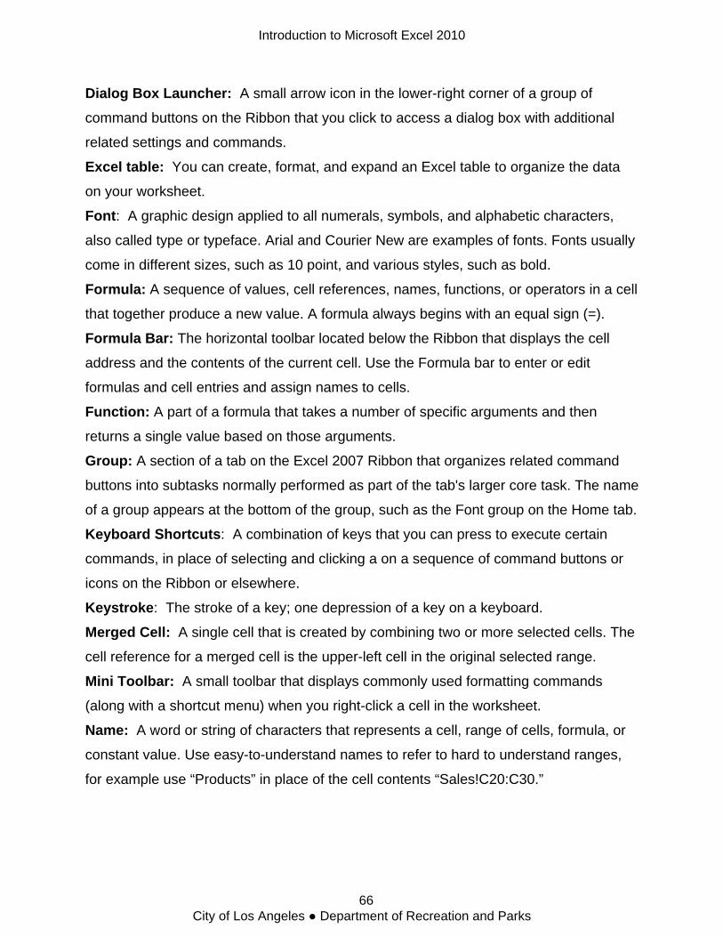
Dialog Box Launcher: A small arrow icon in the lower-right corner of a group of

command buttons on the Ribbon that you click to access a dialog box with additional

related settings and commands.

Excel table: You can create, format, and expand an Excel table to organize the data

on your worksheet. Font: A graphic design applied to all numerals, symbols, and alphabetic characters,

also called type or typeface. Arial and Courier New are examples of fonts. Fonts usually

come in different sizes, such as 10 point, and various styles, such as bold.

Formula: A sequence of values, cell references, names, functions, or operators in a cell

that together produce a new value. A formula always begins with an equal sign (=). Formula Bar: The horizontal toolbar located below the Ribbon that displays the cell

address and the contents of the current cell. Use the Formula bar to enter or edit

formulas and cell entries and assign names to cells.

Function: A part of a formula that takes a number of specific arguments and then

returns a single value based on those arguments.

Group: A section of a tab on the Excel 2007 Ribbon that organizes related command

buttons into subtasks normally performed as part of the tab's larger core task. The name

of a group appears at the bottom of the group, such as the Font group on the Home tab.

Keyboard Shortcuts: A combination of keys that you can press to execute certain

commands, in place of selecting and clicking a on a sequence of command buttons or

icons on the Ribbon or elsewhere.

Keystroke: The stroke of a key; one depression of a key on a keyboard.

Merged Cell: A single cell that is created by combining two or more selected cells. The

cell reference for a merged cell is the upper-left cell in the original selected range. Mini Toolbar: A small toolbar that displays commonly used formatting commands

(along with a shortcut menu) when you right-click a cell in the worksheet.

Name: A word or string of characters that represents a cell, range of cells, formula, or

constant value. Use easy-to-understand names to refer to hard to understand ranges,

for example use “Products” in place of the cell contents “Sales!C20:C30.”



Name box: The left-most section of the Formula bar that identifies the selected cell,

chart item, or drawing object. To name a cell or range, type the name in the Name box

and press ENTER. To move to and select a named cell, click its name in the Name box.

Quick Access toolbar: A small toolbar at the top of the screen and to the right of the

Office button that includes buttons for commands you use often, such as Save and

Undo. You can add buttons to customize the toolbar.

Range: Two or more cells on a sheet. The cells in a range can be adjacent or

nonadjacent. Ribbon: An integrated set of command buttons sorted into tabs by general use, which

appears at the top of the Excel window, just below the title bar. It replaces the menus

and toolbars of previous versions of Excel.

Select: To highlight a cell or range of cells on a worksheet. The selected cells will be

affected by the next command or action.

Select All Button: The gray rectangle in the upper-left corner of a datasheet where the

row and column headings meet. Click this button to select all cells on a worksheet.

ScreenTip: A small window that displays descriptive text when you point to (but do not

click on) a command on the Ribbon or other objects in a worksheet.

Scroll Bars: Horizontal and vertical bars that appear on the bottom and right side of the

worksheet window and enable you to quickly move to a different area of a worksheet.

Sheet Tab scroll buttons: Icons that appear immediately to the left of the sheet tabs in

a workbook, which enable you to bring new tabs into view for worksheets that contain

too many sheets for their tab names to appear at the bottom of a workbook.

Sheet Tabs: Small tabs near the bottom of a worksheet that you click to move between

the worksheets in a workbook. You can assign descriptive names to sheet tabs.

Shortcut Menu: A menu that displays context-sensitive commands when you right-click

a cell or object in a worksheet.

Status bar: A horizontal bar that appears at the bottom of the Excel 2007 window and

keeps you informed of Excel's current mode. In addition, you can use the Status bar to

select a new worksheet view and to zoom in and out on the worksheet.

Tabs: The various "pages" or sections of the Ribbon interface that you click to display

command buttons relating to the tab's name, such as Page Layout and Formulas.



Text box: A rectangular object on a worksheet or chart, in which you can type text. WordArt: Stylized text objects that you use to add pizzazz and emphasis to headings

and other text on your worksheet.

Workbook: The basic file type that you create when you use Excel. A new workbook

consists of three worksheets by default and the worksheets contain rows and columns

in which you can enter and calculate data.

Worksheet: The main document that you work in when you enter data into cells within

Excel, also called a spreadsheet. A worksheet consists of cells that are organized into

columns and rows; a worksheet is always stored in a workbook.

Worksheet area: The portion of a worksheet in which you enter cell data and add

objects such as charts and graphics.



References

Microsoft http://office.microsoft.com

Dummies.com – Excel 2010 http://www.dummies.com/how-to/content/excel-2010-for-dummies-cheat-sheet.html

Dummies.com – Excel 2010 Status Bar http://www.dummies.com/how-to/content/indicators-and-tools-on-the-excel-2010-status-

bar.html

Dummies.com – Excel 2010 Calculations http://www.dummies.com/how-to/content/using-autosum-for-quick-calculations-in-excel-

2010.html

Dummies.com – Excel 2010 Keyboards http://www.dummies.com/how-to/content/how-to-select-excel-2010-commands-with-

keyboard-sh.html#ixzz1DTaGi3mQ

Dummies.com – Excel 2010 Backstage View http://www.dummies.com/how-to/content/using-excel-2010s-file-tab-to-access-

backstage-vie.html#ixzz1DTmY0HLS

About.com - Spreadsheets http://spreadsheets.about.com/od/excelfunctions/qt/autosum.htm

Writings: Milwaukee Public Library – intro to spreadsheets online.



http://office.microsoft.com/

http://www.dummies.com/how-to/content/excel-2010-for-dummies-cheat-sheet.html

http://www.dummies.com/how-to/content/indicators-and-tools-on-the-excel-2010-status-bar.html

http://www.dummies.com/how-to/content/indicators-and-tools-on-the-excel-2010-status-bar.html

http://www.dummies.com/how-to/content/using-autosum-for-quick-calculations-in-excel-2010.html

http://www.dummies.com/how-to/content/using-autosum-for-quick-calculations-in-excel-2010.html

http://www.dummies.com/how-to/content/how-to-select-excel-2010-commands-with-keyboard-sh.html#ixzz1DTaGi3mQ

http://www.dummies.com/how-to/content/how-to-select-excel-2010-commands-with-keyboard-sh.html#ixzz1DTaGi3mQ

http://www.dummies.com/how-to/content/using-excel-2010s-file-tab-to-access-backstage-vie.html#ixzz1DTmY0HLS

http://www.dummies.com/how-to/content/using-excel-2010s-file-tab-to-access-backstage-vie.html#ixzz1DTmY0HLS

http://spreadsheets.about.com/od/excelfunctions/qt/autosum.htm

Notes ____________________________________________________________________________________________________________________________________________________________________________________________________________________________________________________________________________________________________________________________________________________________________________________________________________________________________________________________________________________________________________________________________________________________________________________________________________________________________________________________________________________________________________________________________________________________________________________________________________________________________________________________________________________________________________________________________________________________________________________________________________________________________________________________________________________________________________________________________________________________________________________________________________________________________________________________________________________________________________________________________________________________________________________________________________________________________________________________________________________________________________________________________________________________________________________________________________________________________________________________________________



intro to microsoft excel 2010 to microsoft excel 2010 . ... maximum value of selected numbers. you...

Documents