intro. computer control systems: f1 - introduction · a. emami-naeini, 7th edition, prentice hall....
TRANSCRIPT

Intro. Computer Control Systems:F1
Introduction
Dave Zachariah
Dept. Information Technology, Div. Systems and Control
1 / 20 [email protected]

What is control theory?
The study of dynamical systems and their control.
System = Process = An object whose properties we wish tostudy/control.
Systemoutput(s)input(s)
u y
I The output y is a signal that we can measure and/or wish tocontrol.
I Using the input u we can affect the system and its output.
2 / 20 [email protected]

Dynamical systems
I Static systems: y(t) = f (u(t)), depends on u:s current value!
I Dynamical systems: y(t) may depend on u(τ) for τ ≤ t.
0 10 20 30 40 50 6050
55
60
65
70
75
80
85
90
95
time (s)
thro
ttle
(%
), s
pe
ed
(km
/h)
y(t) = velocity of car
u(t) = throttle
Consequence: Dynamical systems have ‘memory’. Current inputaffects the future output!
3 / 20 [email protected]


Computer control in a nutshell
y
u+ −
Q: Which input u to the motor such that the output y staysaround desired reference signal r = 0◦?
That input u should be computed by a controller!
Design of the controller is the practical goal of control theory
7 / 20 [email protected]

Computer control in a nutshell
y
u+ −
Q: Which input u to the motor such that the output y staysaround desired reference signal r = 0◦?
That input u should be computed by a controller!
Design of the controller is the practical goal of control theory
7 / 20 [email protected]

Computer control in a nutshell
y
u+ −
Q: Which input u to the motor such that the output y staysaround desired reference signal r = 0◦?
That input u should be computed by a controller!
Design of the controller is the practical goal of control theory
7 / 20 [email protected]


Control without feedback
Determine u(t) such that: y(t) should follow a reference signalr(t) closely, despite presence of disturbance v(t).
Open loop: u(t) predetermined by reference r(t).
y(t)u(t)System
v(t)
Controllerr(t)
Challenges:
I Requires accurate knowledge about the system.
I Does not take into account unknown disturbances.
9 / 20 [email protected]

Control without feedback
Determine u(t) such that: y(t) should follow a reference signalr(t) closely, despite presence of disturbance v(t).
Open loop: u(t) predetermined by reference r(t).
y(t)u(t)System
v(t)
Controllerr(t)
Challenges:
I Requires accurate knowledge about the system.
I Does not take into account unknown disturbances.9 / 20 [email protected]

Control using feedback
Feedback: u(t) also determined by measuring y(t).
y(t)u(t)System
v(t)
Controllerr(t)
Advantages:
I Requires only an approximative model of the system.
I Can mitigate unknown disturbances.
Challenges:
I Feedback controller may create instability if poorly designed.
10 / 20 [email protected]

Control using feedback
Feedback: u(t) also determined by measuring y(t).
y(t)u(t)System
v(t)
Controllerr(t)
Advantages:
I Requires only an approximative model of the system.
I Can mitigate unknown disturbances.
Challenges:
I Feedback controller may create instability if poorly designed.10 / 20 [email protected]
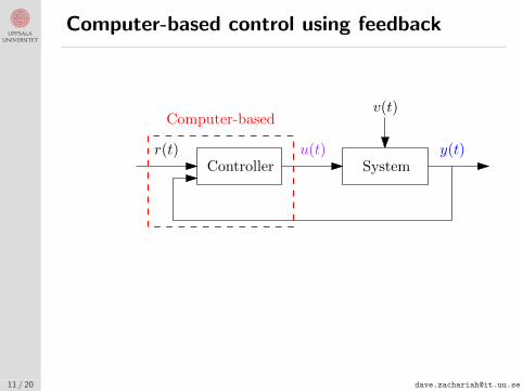
Computer-based control using feedback
y(t)u(t)System
v(t)
Controllerr(t)
Computer-based
Computer-based controller requires:
I Analog-to-digital conversion of y(t)
I Digital-to-analog conversion of u(t)
11 / 20 [email protected]

Computer-based control using feedback
y(t)u(t)System
v(t)
Controllerr(t)
Computer-based
Computer-based controller requires:
I Analog-to-digital conversion of y(t)
I Digital-to-analog conversion of u(t)
11 / 20 [email protected]

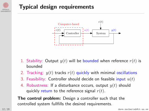
Typical design requirements
y(t)u(t)System
v(t)
Controllerr(t)
Computer-based
1. Stability: Output y(t) will be bounded when reference r(t) isbounded
2. Tracking: y(t) tracks r(t) quickly with minimal oscillations
3. Feasibility: Controller should decide on feasible input u(t)
4. Robustness: If a disturbance occurs, output y(t) shouldquickly return to the reference signal r(t).
The control problem: Design a controller such that thecontrolled system fullfills the desired requirements.
12 / 20 [email protected]


The courseContent
Book options:
I Reglerteknik — Grundlaggande teori, T. Glad & L. Ljung, 4thedition from 2006, Studentlitteratur.
I Feedback Control of Dynamic Systems, G.F. Franklin, J.D. Powell,A. Emami-Naeini, 7th edition, Prentice Hall.
Webpage: http://www.it.uu.se/edu/course/homepage/regsysintro/vt18Studentportalen will also be used.
Content:
I Analysis of linear dynamical systems and feedback
I Basic control principles
I PID controlI Forward- och cascade controlI State feedback control
I Discrete-time models and digital control
14 / 20 [email protected]

The courseExamination forms
Labs:
I 3×Computer Labs (recommended)
I 1×Process Lab (mandatory)
Exam: Evaluation of each problem solution is based on:
1. demonstrating understanding of the problem using principles of thecourse
2. provided a reasonable and reproducible solution
Hand-in (recommended): 2×hand-ins which help getting your handson early and yield bonus credits for the exam.
Secret to passing course
: Get hands dirty
I by taking notes
I through problem solving!
15 / 20 [email protected]

The courseExamination forms
Labs:
I 3×Computer Labs (recommended)
I 1×Process Lab (mandatory)
Exam: Evaluation of each problem solution is based on:
1. demonstrating understanding of the problem using principles of thecourse
2. provided a reasonable and reproducible solution
Hand-in (recommended): 2×hand-ins which help getting your handson early and yield bonus credits for the exam.
Secret to passing course: Get hands dirty
I by taking notes
I through problem solving!
15 / 20 [email protected]


Mathematical models of systems
y(t)u(t)G
Figure: Graphical representation of system G with input and output.
Models are neither ‘true’ nor ‘false’, but rather more or less
I accurate
I useful
representations of underlying mechanisms with measureble effects.
17 / 20 [email protected]

Build intuition from simple systems
Ex. #1: Vehicle in motion
u
y
mFfr
Figure: Force u(t) och velocity y(t).
Physical principles: Newton’s law
F = my,
where F = u− Ffr = u− Cy.[Board: Linear differential equation]
18 / 20 [email protected]
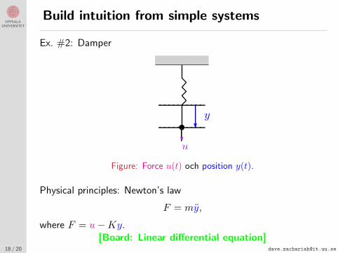
Build intuition from simple systems
Ex. #2: Damper
y
u
Figure: Force u(t) och position y(t).
Physical principles: Newton’s law
F = my,
where F = u−Ky.[Board: Linear differential equation]
18 / 20 [email protected]

Build intuition from simple systems
Ex. #3: Inverted pendulum
y
umg
L
Figure: Torque u(t) och angle y(t).
Physical principles: Torque equation
(mL2/3)y = u+ (mgL/2) sin(y).
Using Taylor series around y = 0:sin(y) ≈ sin(0) + cos(0)(y − 0) = y
[Board: Linear differential equation]18 / 20 [email protected]

Linear system models
Linear time-invariant models are useful and sufficiently accurate inmany control applications
y(t)u(t)G
20 / 20 [email protected]
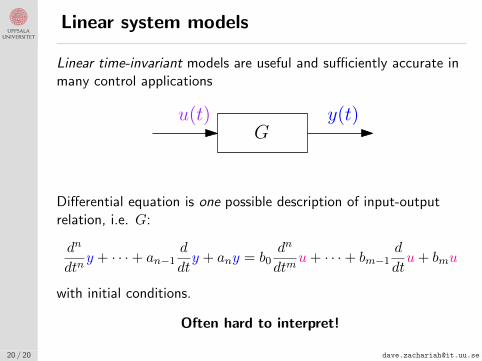
Linear system models
Linear time-invariant models are useful and sufficiently accurate inmany control applications
y(t)u(t)G
Differential equation is one possible description of input-outputrelation, i.e. G:
dn
dtny + · · ·+ an−1
d
dty + any = b0
dn
dtmu+ · · ·+ bm−1
d
dtu+ bmu
with initial conditions.
Often hard to interpret!
20 / 20 [email protected]

Linear system models
Linear time-invariant models are useful and sufficiently accurate inmany control applications
y(t)u(t)G
Different mathematical descriptions of the input-output relation,i.e. G:
1. Differential equations
2. Impulse response / weighting function
3. Transfer function / frequency response
4. State-space description
The latter descriptions are more manageable and practical!
20 / 20 [email protected]

Linear system models
Linear time-invariant models are useful and sufficiently accurate inmany control applications
y(t)u(t)G
Revise basics:
1. Complex numbers
2. Linear ordinary differential equations
3. Laplace transform
4. Linearization using Taylor series expansion
5. Vector/matrix operations and eigenvalues
See Math Tutorial on course webpage!
20 / 20 [email protected]