INTRA-INDUSTRY TRADE AND LABOUR MARKET

ADJUSTMENT IN TURKEY

GUZIN ERLAT AND HALUK ERLAT

Department of Economics

Middle East Technical University 06531 Ankara, Turkey Fax: 90-312-2101244

Email: gerlat@metu.edu.tr herlat@metu.edu.tr

Paper prepared for presentation at the International Conference on Policy Modelling (EcoMod2003) on July 3-5, 2003 at Istanbul.

1. Introduction

Turkey underwent important policy changes in 1980 involving trade

liberalization. As a result her trade, exports in particular, expanded considerably.

Together with this expansion, we also observed a significant increase in intra-industry

trade (IIT) but the dominant characteristic of Turkey’s trade was still inter-industry.

(Erlat and Erlat, 2003). Nevertheless, the question of whether this increase in IIT

contributed to reductions in adjustments costs due to trade expansion needed to be

investigated.

This reduction in costs, called the “smooth-adjustment hypothesis (SAH), is

due to the fact that, movements in the labour market caused by trade expansion will

take place within industries if the share of IIT is high. In fact, measures of IIT have

been used to assess the degree of structural adjustment required by trade expansion. In

a previous paper, (Erlat and Erlat, 2003), we made use of IIT measures in this sense.

The measures we utilized for this purpose evaluated the share or level of IIT in new

trade and are called Marginal IIT (MIIT) measures. This concept and a measure were

first introduced into the literature by Hamilton and Kniest (1991). Improved measures

were later developed by Brülhart (1994) and it was his C-index, which measures the

level of MIIT that we used in our paper. In doing so, we operated under the

simplifying assumption that changes in adjustment costs (measured as changes in

employment) were exactly matched by the changes in trade flows1.

In this paper, we undertake an econometric approach to testing SAH. Such

studies are rather limited in number. A number of them may be found in Brulhart and

Hine (1999) but the majority of these studies only investigate simple correlations

between employment changes and measures of IIT and MIIT. As to the econometric

studies; the problem is investigated for Belgium by Tharakan and Calfat (1999), for

Greece by Sarris, Papadimitriou and Mavrogiannis (1999), for Ireland by Brülhart

(2000), for Malaysia by Brulhart and Thorpe (2000), and for the U.K. by Brulhart and

Elliott (2002) and Greenaway, Hines and Milner (2002). Evidence in favour of the

SAH is found for Ireland and Greece, but none for Belgium and Malaysia. The

evidence for the U.K. is mixed. Brulhart and Elliott (2002) find evidence in favour of

1

the SAH and, also in favour of using MIIT indexes instead of an IIT index to

represent the contribution that intra-industry trade makes, while Greenaway et al.

(2002: 271) conclude that there is no evidence of “… a systematic relationship

between the type of trade expansion (inter- or intra-industry) and the type of

employment adjustment (within or between industry adjustment) or that there is less

labour market adjustment associated with intra- than inter-industry trade.”

All countries cited above are developed except Malaysia. Both because the

Turkish economy is closer, in this respect, to the Malaysian economy and because we

do not have access to the data on some of the variables (the proxies for the dependent

variable, in particular) used by Brülhart (2000), Brülhart and Elliot (2002) and

Greenaway et al. (2002) (which are the more sophisticated of the econometric

applications listed above), we have applied the model in Brülhart and Thorpe (2000)

to Turkish data. Thus, in the next section, we give some information about the intra-

industry structure of Turkish international trade and, in doing so, also introduce the

measures of IIT and MIIT that we shall utilize. In section 3, the model will be

specified. The data used in the econometric application will be described in Section 4

and the empirical results will be presented. Section 5 will contain our conclusions.

2. Intra-Industry Structure of Turkish Trade

In Erlat and Erlat (2003) we extensively investigated the IIT structure of

Turkish international trade, based on 3-digit SITC (Rev. 3) data. In the present case,

we needed to use an industrial classification; hence, the trade data that we shall base

our analysis upon will be for 3-digit ISIC (Rev. 2) industrial sectors. They cover the

period 1969-2001 and are measured in $US. They were obtained from the State

Institute of Statistics (SIS) database.

We first present the plots of total exports (X) and imports (M) in Figure 1a

and, of manufacturing industry exports (XMI) and imports (MMI) in Figure 1b. We

note that (a) imports always exceed exports in both cases, (b) even though imports

show a steady growth from the beginning of the period, the growth of exports pick-up

1 Brulhart (1999) contains a simplified model where this holds. The link between MIIT and adjustment costs is also discussed theoretically by Azhar, Elliot and Milner (1998) and Lovely and Nelson (2000, 2002).

2

after 1980, and (c) the post-1980 growth in exports appears to be dominated by the

growth in the exports of manufacturing industries.

Subsequently, we calculated the Grubel and Lloyd (GL) (1971) index for each

3-digit industry. Letting Xit and Mit stand for the exports and imports of industry i in

period t, respectively, the GL index for the ith industry at time t may be expressed as

0

10000

20000

30000

40000

50000

60000

70 75 80 85 90 95 00

X M

0

10000

20000

30000

40000

50000

70 75 80 85 90 95 00

XMI MMI

Figure 1aPlot of Total Exports (X) and Total Imports (M)

Figure 1bPlot of Manufacturing Industry Exports (XMI) and Imports (MMI)

(1) T,,1t;N,,1i,MXMX

1GLitit

ititit KK ==

+

−−=

GLit lies between 0 and 1, with values close to unity indicating a high rate of IIT for

the ith industry. We may aggregate the GLit across industries by obtaining its

weighted average, using the shares of each industry in total trade as the weights. The

resultant expression becomes,

3

(2) T,,1t,)MX(

MX1GL N

1iitit

N

1iitit

t

____K=

+

−−=

∑

∑

=

=

We calculated GL for both total trade and trade in manufactured products.

The plots of both indexes are given in Figure 2. We note that the rate of IIT was low

and declining prior top 1980, after which we observe a rapid increase, particularly in

the manufacturing industries, until 1986, after which it slightly declines to its pre-

1985 level, picking-up again after 1994. Again, the manufacturing sector appears to

be instrumental in the rise of IIT.

t

____

0.0

0.1

0.2

0.3

0.4

0.5

0.6

70 75 80 85 90 95 00

GL GLMI

Figure 2Plot of the Average GL Index for all 3-digit Sectors and the Average GL index for Manufacturing Industries

Finally, we used Brulhart (1994)’s A-index to measure MIIT for each

industry. Let Xit and Mit, again, denote the exports and imports of industry i at period

t, and let Xi,t-n and Mi,t-n be the exports and imports of i at period t-n where .

Denote X

1n ≥

it - Xi,t-n by ∆Xin and Mit - Mi,t-n by ∆Min2. Then, the A-index may be

expressed as,

2 The X and M’s are now measured in real terms since the MIIT indexes measure real changes in trade flows. We, thus, expressed all series in TL terms using period-average exchange rate series and, subsequently, adjusted them for inflation using the 1987 based Wholesale Price Index (WPI). The exchange rate and WPI series were obtained from the Central Bank database.

4

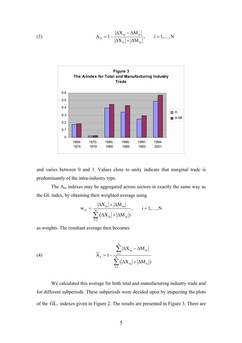
(3) N,,1i,MXMX

1Ainin

ininin K=

∆+∆

∆−∆−=

Figure 3 The A-Index for Total and Manufacturing Industry

Trade

0

0.1

0.2

0.3

0.4

0.5

0.6

1969-1974

1975-1979

1980-1985

1986-1989

1990-1993

1994-2001

A

A-MI

and varies between 0 and 1. Values close to unity indicate that marginal trade is

predominantly of the intra-industry type.

The Ain indexes may be aggregated across sectors in exactly the same way as

the GL index, by obtaining their weighted average using

N,,1i,)MX(

MXw N

1iinin

ininin K=

∆+∆

∆+∆=

∑=

as weights. The resultant average then becomes

(4) )MX(

MX1A N

1iinin

N

1iinin

n

∑

∑

=

=

∆+∆

∆−∆−=

We calculated this average for both total and manufacturing industry trade and

for different subperiods. These subperiods were decided upon by inspecting the plots

of the GL indexes given in Figure 2. The results are presented in Figure 3. There are t

____

5

two subperiods prior to 1980 and we note that MIIT is less than 20% in both of them;

in fact, it is even lower than 5% for the 1975-1979 period. Things improve

considerably after 1980. The largest jump is in the 1980-85 period. There is some

decline in the next two periods. This decline is more pronounced in the MIIT

component of total trade compared to that of manufacturing industry trade. However,

during the last period, 1994-2001, we observe a significant increase in MIIT,

particularly in manufacturing industry trade.

To sum up; the Turkish economy has exhibited considerable expansion in its

international trade after 1980 and both IIT and MIIT have shown appreciable increase

as a result of this expansion. The manufacturing sector appears to be the primary

mover in all these developments.

3. The Model

As mentioned in the Introduction, we follow Brulhart and Thorpe (2000) and

estimate the following two specifications of an equation designed to account for

changes in employment in 3-digit ISIC (Rev. 2) manufacturing industries:

(5) LDEMPLit = β0 + β1 LDCONSit + β2 LDPRODit + β3 LTREXit + β4 IITit + uit

and

(6) LDEMPLit = β0 + β1 LDCONSit + β2 LDPRODit + β3 LTREXit + β4 IITit

+ β5 (IITxLTREX)it + uit

where uit = µi + εit and εit ∼iid(0, σ2). We assume the cross-section component µi to be

fixed since the 3-digit industries that make-up the panel have not been chosen at

random. Hence, both specifications are estimated using a fixed effects estimator that

is, basically, OLS with cross-section dummies.

The variables used may be defined as follows:

LDEMPL = The natural log of the absolute value of the change in

employment (L) between t and t-n.

6

LDCONS = The natural log of the absolute value of the change in

apparent consumption (C = Q + X – M) between t and

t-n, Q being output.

LDPROD = The natural log of the absolute value of the change in

labour productivity, measured as output per worker,

between t and t-n.

LTREX = The natural log of trade exposure [(X+M)/Q].

IIT = May be GL, ∆GL or A.

IITxLTREX = The interaction between IIT and trade exposure.

LDEMPL is a proxy for the costs of adjustment in the labour market. The

assumption is that the costs of moving labour across industries is proportional to the

size of net changes in wage payments and, furthermore, that this proportion is the

same for all industries and over time. The expected sign for the coefficient of

LDCONS is positive. One would expect the coefficient of LDPROD to be negative

since increases in productivity would tend to reduce the labour requirement to

produce the same level of output. This expectation is supported by evidence from the

accounting measure of employment change found in, e.g., Tharakan and Calfat (1999)

for Belgium, Sarris et al. (1999) for Greece and Erlat (2000) for Turkey. The prior

expectation for the coefficient of LTREX is that it should be positive since trade

exposure is expected to increase inter-industry specialization pressures (Brulhart and

Thorpe, 2000: 730). Finally, the coefficients of both IIT and IITxLTREX are expected

to be negative given the smooth adjustment hypothesis. The reason for the

introduction of IITxLTREX in the second specification is the expectation that IIT

should matter more in sectors where the level of trade is high.

4. Empirical Results

The data used to measure the variables defined above were all obtained from

the SIS database. The non-trade data are based on their annual Census of Industrial

Production. This data was only available for the period 1974-1999; hence, we

considered it in the estimations. This, however, is not an important shortcoming since

the rate of IIT starts reaching meaningful levels after 1980. All data have been

deflated using the 1987-based WPI.

7

We used three proxies for the IIT variable. These are, the A-index for MIIT,

the change in the GL index, ∆GL, and the GL index itself. The A index and ∆GL have

been calculated as yearly changes and three-yearly changes. It has been shown by

Oliveras and Terra (1997) that A-indexes calculated for subintervals of a given

interval cannot be aggregated to the A index for the parent interval unless the net

balance of trade changes has the same sign in all subintervals. Since this situation may

be the exception rather than the rule, choice of interval in calculating the A index is

important. Brulhart (1999) has investigated this question within the context of testing

the SAH and has reached the conclusion that A indexes based on yearly changes give

the best results. But, A indexes based on yearly changes would show a lot of

volatility; so we also carried out our estimations using three-yearly changes which are

expected to show a smoother picture.

Of course, in the case of three-yearly changes, the variables that enter the

model as levels, namely, LTREX and GL, had to be calculated accordingly, and this

was done by computing their subperiod averages.

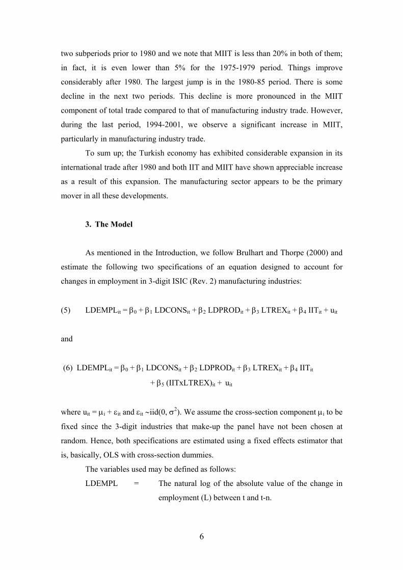
The estimates based on yearly changes are given in Table 1. We find that (a) the

coefficient of IIT is positive in all specifications and for all proxies except for the

coefficient of GLxLTREX; this estimate, however, is not statistically significant, (b)

the coefficient of the A-index, even though positive, is statistically significant in the

specification with the interaction term and so is the coefficient of the interaction term,

(c) the coefficients of ∆GL and ∆GLxLTREX are positive but statistically

insignificant, while the coefficient of GL in the model without an interaction term is

positive and significant, but becomes insignificant when GLxLTREX is introduced.

These results are the reverse of what is expected when testing the SAH and appear to

be closer to what Brulhart and Thorpe (2000) found for Malaysia. They call their

findings for Malaysia “puzzling” but, in view of Tharakan and Calfat (1999) and

Greenaway et al. (2002)’s empirical results and Lovely and Nelson (2000, 2002)’s

theoretical predictions, neither their findings, nor ours may be unexpected. In fact,

Lovely and Nelson (2000) construct a model where the change in total trade is all

intra-industry but labour adjustment is all inter-industry. Thus, our expectations

regarding the sign of the coefficient of A need not be so strong.

8

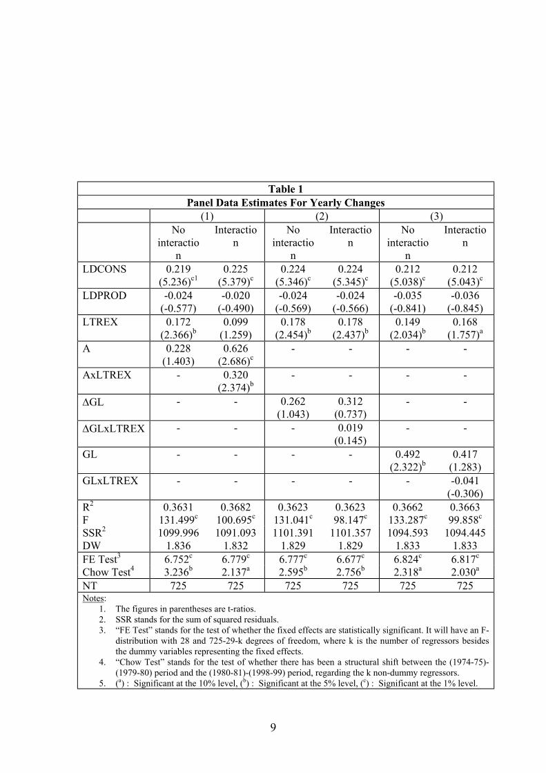
Table 1 Panel Data Estimates For Yearly Changes

(1) (2) (3) No

interaction

Interaction

No interactio

n

Interaction

No interactio

n

Interaction

LDCONS 0.219 (5.236)c1

0.225 (5.379)c

0.224 (5.346)c

0.224 (5.345)c

0.212 (5.038)c

0.212 (5.043)c

LDPROD -0.024 (-0.577)

-0.020 (-0.490)

-0.024 (-0.569)

-0.024 (-0.566)

-0.035 (-0.841)

-0.036 (-0.845)

LTREX 0.172 (2.366)b

0.099 (1.259)

0.178 (2.454)b

0.178 (2.437)b

0.149 (2.034)b

0.168 (1.757)a

A 0.228 (1.403)

0.626 (2.686)c

- - - -

AxLTREX - 0.320 (2.374)b

- - - -

∆GL - - 0.262 (1.043)

0.312 (0.737)

- -

∆GLxLTREX - - - 0.019 (0.145)

- -

GL - - - - 0.492 (2.322)b

0.417 (1.283)

GLxLTREX - - - - - -0.041 (-0.306)

R2 0.3631 0.3682 0.3623 0.3623 0.3662 0.3663 F 131.499c 100.695c 131.041c 98.147c 133.287c 99.858c

SSR2 1099.996 1091.093 1101.391 1101.357 1094.593 1094.445 DW 1.836 1.832 1.829 1.829 1.833 1.833 FE Test3 6.752c 6.779c 6.777c 6.677c 6.824c 6.817c

Chow Test4 3.236b 2.137a 2.595b 2.756b 2.318a 2.030a

NT 725 725 725 725 725 725 Notes:

1. The figures in parentheses are t-ratios. 2. SSR stands for the sum of squared residuals. 3. “FE Test” stands for the test of whether the fixed effects are statistically significant. It will have an F-

distribution with 28 and 725-29-k degrees of freedom, where k is the number of regressors besides the dummy variables representing the fixed effects.

4. “Chow Test” stands for the test of whether there has been a structural shift between the (1974-75)-(1979-80) period and the (1980-81)-(1998-99) period, regarding the k non-dummy regressors.

5. (a) : Significant at the 10% level, (b) : Significant at the 5% level, (c) : Significant at the 1% level.

9

The coefficient of LDCONs is positive in all cases and they are all statistically

significant. On the other hand, the coefficient of LDPROD is negative in all cases but

they are all statistically insignificant. Finally, the coefficient of the trade exposure

variable, LTREX, is positive in all cases and is statistically significant except in the

specification with an interactive term and the A-index used as a proxy for IIT.

We also performed two sets of tests for both specifications. The first is a test

of whether the fixed effects specification is valid. We find this specification to hold in

all cases. The second test, the Chow test, is used to test if the coefficients of the

regressors, LDCONS, LDPROD, LTREX, IIT and IITxLTREX, are the same for the

subperiods (1974-75)-(1979-80) and (1980-81)-(1998-99). The outcomes of the test,

in all cases, indicate that a statistically significant structural shift has occurred after

1980. This shift, apparently, is due to a significant shift in the coefficient of

LDPROD, turning it from a positive value to a negative one.3

The estimates based on three-yearly changes are presented in Table 2. The

coefficient of LDCONS is again positive and significant while the coefficient of

LDPROD is negative and insignificant, in all cases. The coefficient of LTREX is

again positive but, now, is statistically insignificant in all cases. As for the IIT

proxies, we find the coefficient of A to be, again, positive but, now, significant in both

specifications. The interactions term, however, is not significant. The coefficients

associated with ∆GL and GL are all insignificant and, all but the coefficient of ∆GL in

the first specification, are positive. The validity of the fixed effects is confirmed, once

again, by the appropriate test. We did not perform a test for structural change in this

case because the time-wise subsamples involved were rather small to provide us with

meaningful results.

We also considered subsets of the manufacturing industries that exhibited high

IIT and MIIT rates. To determine these subsets we first calculated the means of the

GLit and Ait over the period 1980-2001 and then took the average of these means

across industries. Industries with time-wise means greater than these averages were

chosen. The industries in question are given in Table 3. The first column has the

industries with high IIT rates, while the second column has the industries with high

3 The estimates of the model with structural shift dummies are available upon request. We also estimated the two models for the (1980-81)-(1998-99) subperiod. The results were similar to the ones obtained for the full period and are not repeated here. They, also, are available upon request.

10

MIIT rates. The final column contains the industries with both high IIT and MIIT

rates. We note that the intersection of the high IIT industry set and the high MIIT

Table 2 Panel Data Estimates For Three-Yearly Changes

(1) (2) (3) No

interaction

Interaction

No interactio

n

Interaction

No interactio

n

Interaction

LDCONS 0.193 (2.501)b1

0.176 (2.268)b

0.209 (2.693)c

0.210 (2.716)c

0.208 (2.636)c

0.205 (2.583)c

LDPROD -0.036 (-0.447)

-0.036 (-0.453)

-0.032 (-0.402)

-0.029 (-0.367)

-0.032 (-0.395)

-0.028 (-0.346)

LTREX 0.099 (0.737)

0.067 (0.492)

0.164 (1.237)

0.143 (1.077)

0.163 (1.197)

0.100 (0.528)

A 0.518 (2.117)b

0.900 (2.404)b

- - - -

AxLTREX - 0.312 (1.347)

- - - -

∆GL - - -0.141 (-.0455)

0.629 (1.049)

- -

∆GLxLTREX - - - 0.373 (1.498)

- -

GL - - - - 0.003 (0.008)

0.256 (0.388)

GLxLTREX - - - - - 0.177 (0.483)

R2 0.4872 0.4919 0.4762 0.4821 0.4757 0.4763 F 60.027c 47.915c 60.308c 46.075c 60.177c 45.017c

SSR2 234.291 232.164 239.317 236.635 239.564 239.282 DW 1.945 1.958 1.966 1.964 1.976 1.980 FE Test3 3.159c 3.236c 3.047c 3.073c 3.035c 3.003c

NT 232 232 232 232 232 232 Notes:

1. The figures in parentheses are t-ratios. 2. SSR stands for the sum of squared residuals. 3. “FE Test” stands for the test of whether the fixed effects are statistically significant. It will have an F-

distribution with 28 and 232-29-k degrees of freedom, where k is the number of regressors besides the dummy variables representing the fixed effects.

4. (a) : Significant at the 10% level, (b) : Significant at the 5% level, (c) : Significant at the 1% level.

industry set is not very large, implying that the correlation between the GL and A

indexes is relatively low.

We estimated the two specifications given in equations (5) and (6) for all three

subsets using yearly changes. The results are presented in Table 4 and contain only

11

the coefficient estimates of the three IIT proxies, A, ∆GL and GL. The coefficient of

LDCONS is positive and significant, while the coefficient of LDPROD is negative

and

Table 3 Industries with High IIT and/or MIIT Rates

(a) (b) (c) 311 Food manufacturing 311 Food manufacturing 311 Food manufacturing 314 Tobacco manufactures 313 Beverage industries 314 Tobacco manufactures 323 Manufacture of leather and products of leather, leather substitutes and fur, except footwear and wearing apparel

314 Tobacco manufactures 323 Manufacture of leather and products of leather, leather substitutes and fur, except footwear and wearing apparel

324 Manufacture of footwear, except vulcanized or molded rubber or plastic footwear

321 Manufacture of textiles 324 Manufacture of footwear, except vulcanized or molded rubber or plastic footwear

331 Manufacture of wood and wood and cork products, except furniture

323 Manufacture of leather and products of leather, leather substitutes and fur, except footwear and wearing apparel

356 Manufacture of plastic products not elsewhere classified

332 Manufacture of furniture and fixtures, except primarily of metal

324 Manufacture of footwear, except vulcanized or molded rubber or plastic footwear

371 Iron and steel basic industries

353 Petroleum refineries 341 Manufacture of paper and paper products

372 Non-ferrous metal basic industries

356 Manufacture of plastic products not elsewhere classified

342 Printing, publishing and allied industries

381 Manufacture of fabricated metal products, except machinery and equipment

361 Manufacture of pottery, china and earthenware

351 Manufacture of industrial chemicals

390 Other Manufacturing Industries

369 Manufacture of other non-metallic mineral products

352 Manufacture of other chemical products

371 Iron and steel basic industries 356 Manufacture of plastic products not elsewhere classified

372 Non-ferrous metal basic industries

362 Manufacture of glass and glass products

381 Manufacture of fabricated metal products, except machinery and equipment

371 Iron and steel basic industries

390 Other Manufacturing Industries 372 Non-ferrous metal basic industries

381 Manufacture of fabricated metal products, except machinery and equipment

382 Manufacture of machinery except electrical

383 Manufacture of electrical machinery apparatus, appliances and supplies

390 Other Manufacturing Industries

insignificant in all cases considered. The coefficient of LTREX is also positive

throughout but its statistical significance varies.4

4 The detailed estimation results are available upon request.

12

We note that we now have a few negative coefficient estimates but only one of

these, the coefficient of GLxLTREX for the subset with high MIIT rates, is

significantly different from zero, but only at the 10% level of significance. It is hard

to claim that this constitutes evidence in favour of the smooth adjustment hypothesis.

The

Table 4 Panel Data Estimates for Subgroups of Industries Based on Yearly Changes

(a) (b) (c) No

interaction

Interaction

No interactio

n

Interaction

No interactio

n

Interaction

A1 0.217 (1.015)2

0.667 (1.859)a

0.185 (0.954)

0.408 (1.392)

0.275 (1.018)

0.652 (1.295)

AxTREX - 0.344 (1.561)

- 0.192 (1.014)

- 0.368 (0.886)

∆GL -0.112 (-0.370)

0.679 (1.279)

0.917 (2.452)b

0.126 (0.201)

0.708 (1.457)

-0.108 (-0.106)

∆GLxTREX - 0.405 (1.815)a

- -0.436 (-1.566)

0.708 (1.457)

-0.671 (-0.910)

GL 0.306 (1.241)

0.811 (1.929)a

0.710 (2.421)b

-0.0003 (-0.0005)

0.591 (1.607)

0.865 (1.136)

GLxTREX - 0.338 (1.481)

- -0.469 (-1.890)a

- 0.214 (0.410)

N 15 15 18 18 9 9 T 25 25 25 25 25 25 NT 375 375 450 450 225 225 Notes:

1. The estimates are obtained from models that contain, in addition to the IIT proxies, LDCONS, LDPROD and LTREX as explanatory variables. The estimates pertaining to their coefficients are not presented in order to focus on the IIT proxies.

2. The figures in parentheses are t ratios. 3. (a) : Significant at the 10% level, (b) : Significant at the 5% level, (c) : Significant at the 1% level.

rest of the coefficient estimates are again positive and the strongest results are found

for the high MIIT subset but for the coefficients of ∆GL and GL, not, as one would

expect, for the coefficient of A.

5. Conclusions

In this paper, we sought to test the smooth adjustment hypothesis based on an

econometric model previously estimated by Brulhart and Thorpe (2000) for

13

Malaysia. We used panel data based on the ISIC (Rev.2) classification. We may list

our conclusions as follows:

1. We considered the period (1974-75)-(1998-99) and found, when all

manufacturing industries were considered, that the coefficients of the IIT proxies

were all positive except for one (GLxLTREX) which was, nevertheless, statistically

insignificant. Although this result appears to go against expectation, whether this

expectation is always warranted is open to question. All IIT proxies, A included, are

production based measures. But, as Lovely and Nelson (2002: 192) argue, “... changes

in trade patterns reflect changes in production and demand.” Hence, the expected sign

of the changes in employment due to IIT may not, necessarily, be negative.

2. Coefficients that were positive and statistically significant were obtained

using the A and GL indexes, but not ∆GL.

3. In the results based on three-yearly changes, there was again only one

negative but statistically insignificant coefficient (∆GL in the model with no

interaction). Of the positive coefficients, only those associated with the A-index were

significant.

4. We also repeated the estimations for subsets of the industries with high IIT

and/or MIIT rates. In this case, we were able to obtain more significant results but

only one of these was negative. We also noted that now both ∆GL and GL appeared

to indicate stronger relationships with changes in employment.

5. In sum, we were able to obtain some evidence of a significant relationship

between employment changes and IIT but, if we adhered to the strict expectation that

such a relationship should be negative, then we would have to agree with Brulhart and

Thorpe (2000) that this evidence is “puzzling”. But there are both empirical and

theoretical grounds for us to not entertain such a strict prior.

References

Azhar, A.K.M., R.J.R. Elliot and R.C. Milner (1998): “Static and Dynamic Measurement of Intra-Industry Trade and Adjustment: A Geometric Appraisal”, Weltwirtschaftliches Archiv, 134, 404-422.

Brulhart, M. (1994): “Marginal Intra-Industry Trade: Measurement and Relevance for

the Pattern of Industrial Adjustment”, Weltwirtschaftliches Archiv, 130, 600-613.

14

Brulhart, M. (1999): “Marginal Intra-Industry Trade and Trade-Induced Adjustment: A Survey” in M. Brulhart and R.C. Hine (eds.): Intra-Industry Trade and Adjustment: The European Experience. London: Macmillan Press, 36-69.

Brulhart, M. (2000): “Dynamics of Intra-Industry Trade and Labour Market

Adjustment”, Review of International Economics, 8, 420-435. Brulhart, M. and R.J.R. Elliott (2002): “Labour Market Effects of Intra-Industry

Trade: Evidence for the United Kingdom”, Weltwirtschaftliches Archiv, 138, 207-228.

Brulhart, M. and R.C. Hine (eds.) (1999): Intra-Industry Trade and Adjustment: The

European Experience. London: Macmillan Press. Brulhart, M. and M. Thorpe (2000): “Intra-Industry Trade and Adjustment in

Malaysia: Puzzling Evidence”, Applied Economics Letters, 7, 729-733. Erlat, G. (2000): “Measuring the Impact of Trade Flows on Employment in the

Turkish Manufacturing Industry”, Applied Economics, 32, 1169-1180. Erlat, G. and H. Erlat (2003): “Measuring Intra-Industry and Marginal Intra-Industry

Trade: The Case for Turkey”, forthcoming in the November-December 2003 issue of Emerging Markets Finance and Trade.

Greenaway, D., M. Haynes and C. Milner (2002): “Adjustment, Employment

Characteristics and Intra-Industry Trade”, Weltwirtschaftliches Archiv, 138, 254-276.

Grubel, H. and P.J. Lloyd (1971): “The Empirical Measurement of Intra-Industry

Trade”, Economic Record, 470, 494-517. Hamilton, C. and P. Kniest (1991): “Trade Liberalization, Structural Adjustment and

Intra-Industry Trade”, Weltwirtschaftliches Archiv, 127, 356-367. Lovely, M.E. and D.R. Nelson (2000): “Marginal Intra-Industry Trade and Labour

Adjustment”, Review of International Economics, 8, 436-477. Lovely, M.E. and D.R. Nelson (2002): “Intra-Industry Trade as an Indicator of

Labour Market Adjustment”, Weltwirtschaftliches Archiv, 138, 179-206. Oliveras, J. and I. Terra (1997): “Marginal Intra-Industry Trade Index: The Period and

Aggregation Choice”, Weltwirtschaftliches Archiv, 133, 170-179. Sarris, A.H., P. Papadimitriou and A. Mavrogiannis (1999): “Greece” in M. Brulhart

and R.C. Hine (eds.): Intra-Industry Trade and Adjustment: The European Experience. London: Macmillan Press, 168-187.

15

Tharakan, P.K.M., and G. Calfat (1999): “Belgium” in M. Brulhart and R.C. Hine (eds.): Intra-Industry Trade and Adjustment: The European Experience. London: Macmillan Press, 121-134.

16