interval estimation for parameters of a bivariate time ... papers/jst vol. 17 (2) jul....

ISSN: 0128-7680Pertanika J. Sci. & Technol. 17 (2): 313 – 323 (2009) © Universiti Putra Malaysia Press

Received: 7 May 2008Accepted: 14 October 2008

Interval Estimation for Parameters of a Bivariate Time Varying Covariate Model

Jayanthi ArasanDepartment of Mathematics, Faculty of Science,

Universiti Putra Malaysia, 43400 UPM, Serdang, Selangor, Malaysia

E-mail:[email protected]

ABSTRACTThis paper investigates several asymptotic confidence interval estimates, based on the Wald, likelihood ratio and the score statistics for the parameters of a parallel two-component system model, with dependent failure and a time varying covariate, when data is censored. This model is an extension of the bivariate exponential model. The procedures are investigated via a coverage probability study using the simulated data. The results clearly indicate that the interval estimates, based on the likelihood ratio method, work better than any of the other two methods when dealing with the censored data.

Keywords: Bivariate, time varying, censoring, covariates, asymptotic, Wald, parallel, score

INTRODUCTIONThe main limitation for most models, with censored data, is the fact that exact confidence intervals are impossible to compute. One alternative is to use large sample intervals, based on the asymptotic normality of the maximum likelihood estimates. However, there are some concerns over the use of the intervals which are based on asymptotic normality. Jeng and Meeker (2000) pointed out that its actual coverage probability could be significantly different from the nominal specification for a small to moderate number of failures, particularly for the one-sided confidence bounds. Cox and Hinkley (1979) mentioned that one of the disadvantages of using the Wald statistic is that it is not invariant under the transformation of the parameter of interest, unlike the methods which are based on the likelihood ratio and the score tests. This paper investigates the interval estimates based on the Wald, likelihood ratio and the score methods, when they are applied to the parameters of the bivariate exponential model with dependent failure, time varying covariate and censored data. This is an extension of the bivariate exponential model by Freund (1961). Most of the studies, with parametric models involving time varying covariates, are in the area of political science and sociology. Works involving time varying covariates and duration dependence were done and discussed by authors such as Petersen (1986), Beck (1999), Bennet (1999), Box-Steffensmeier and Jones (1997), Tuma and Hannan (1984), Blossfield et al. (1989), Yamaguchi (1991), Courgeau and Leli e vre (1992), as well as Kalbfleisch and Prentice (1980).

Jayanthi Arasan

314 Pertanika J. Sci. & Technol. Vol. 17 (2) 2009

MATERIALS AND METHODS

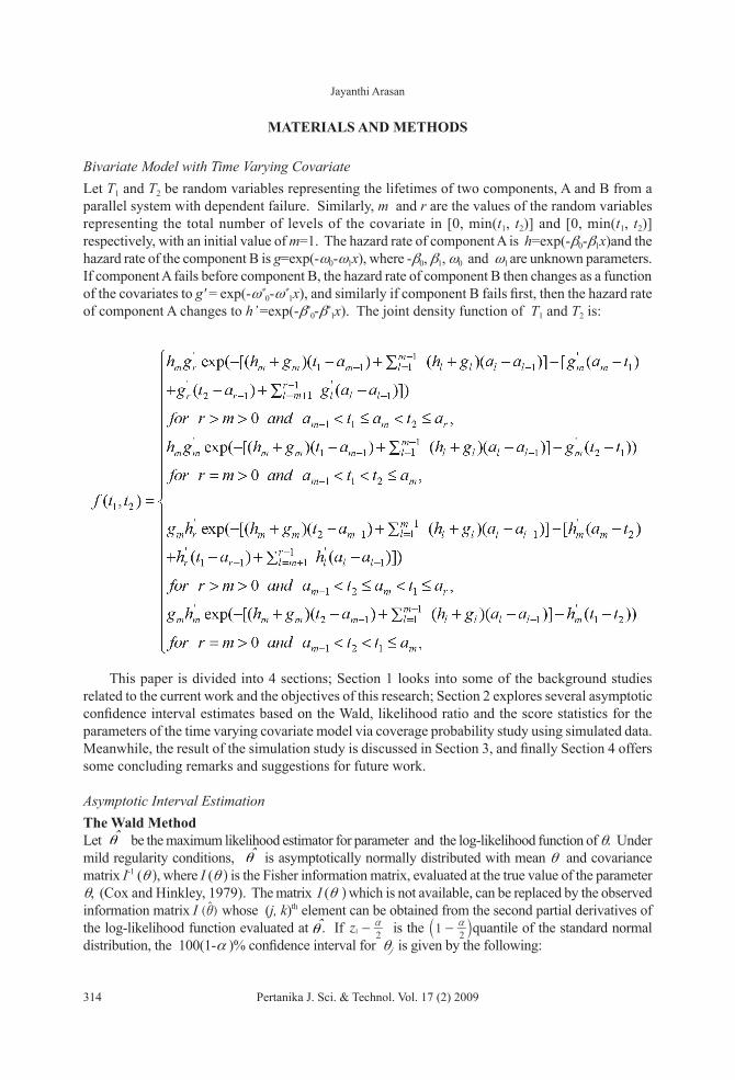
Bivariate Model with Time Varying CovariateLet T1 and T2 be random variables representing the lifetimes of two components, A and B from a parallel system with dependent failure. Similarly, m and r are the values of the random variables representing the total number of levels of the covariate in [0, min(t1, t2)] and [0, min(t1, t2)] respectively, with an initial value of m=1. The hazard rate of component A is h=exp(-b0-b1x)and the hazard rate of the component B is g=exp(-w0-w1x), where -b0, b1, w0 and w1 are unknown parameters. If component A fails before component B, the hazard rate of component B then changes as a function of the covariates to g' = exp(-w*

0-w*1x), and similarly if component B fails first, then the hazard rate

of component A changes to h’ =exp(-b*0-b*

1x). The joint density function of T1 and T2 is:

This paper is divided into 4 sections; Section 1 looks into some of the background studies related to the current work and the objectives of this research; Section 2 explores several asymptotic confidence interval estimates based on the Wald, likelihood ratio and the score statistics for the parameters of the time varying covariate model via coverage probability study using simulated data. Meanwhile, the result of the simulation study is discussed in Section 3, and finally Section 4 offers some concluding remarks and suggestions for future work.

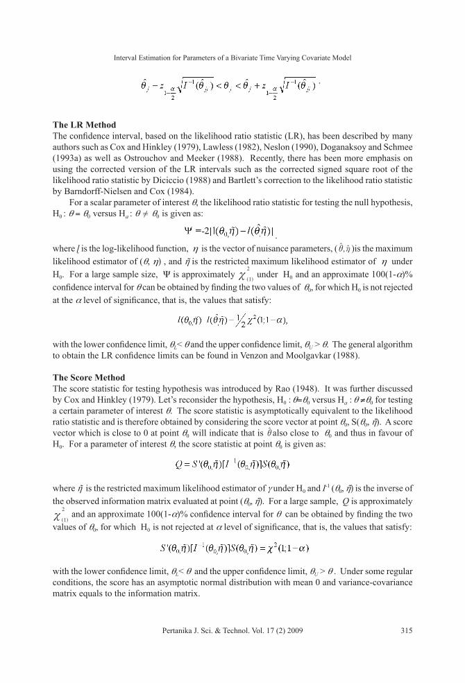
Asymptotic Interval EstimationThe Wald MethodLet θ be the maximum likelihood estimator for parameter and the log-likelihood function of θ. Under mild regularity conditions, θ is asymptotically normally distributed with mean θ and covariance matrix I-1 (θ ), where I (θ ) is the Fisher information matrix, evaluated at the true value of the parameter θ, (Cox and Hinkley, 1979). The matrix I (θ ) which is not available, can be replaced by the observed information matrix I ( )it whose (j, k)th element can be obtained from the second partial derivatives of the log-likelihood function evaluated at . If z

21

a- is the 1

2

a-a kquantile of the standard normal

distribution, the 100(1-α )% confidence interval for θj is given by the following:θ


Pertanika J. Sci. & Technol. Vol. 17 (2) 2009 315

.

The LR MethodThe confidence interval, based on the likelihood ratio statistic (LR), has been described by many authors such as Cox and Hinkley (1979), Lawless (1982), Neslon (1990), Doganaksoy and Schmee (1993a) as well as Ostrouchov and Meeker (1988). Recently, there has been more emphasis on using the corrected version of the LR intervals such as the corrected signed square root of the likelihood ratio statistic by Diciccio (1988) and Bartlett’s correction to the likelihood ratio statistic by Barndorff-Nielsen and Cox (1984). For a scalar parameter of interest θ, the likelihood ratio statistic for testing the null hypothesis, H0 : θ = θ0 versus Ha : θ ! θ0 is given as:

.where ɭ is the log-likelihood function, h is the vector of nuisance parameters, ( ,i ht t )is the maximum likelihood estimator of (θ, h) , and ῆ is the restricted maximum likelihood estimator of h under H0. For a large sample size, Y is approximately

( )1

2

| under H0 and an approximate 100(1-α)%

confidence interval for θ can be obtained by finding the two values of θ0, for which H0 is not rejected at the α level of significance, that is, the values that satisfy:

with the lower confidence limit, θL< θ and the upper confidence limit, θU > θ. The general algorithm to obtain the LR confidence limits can be found in Venzon and Moolgavkar (1988).

The Score MethodThe score statistic for testing hypothesis was introduced by Rao (1948). It was further discussed by Cox and Hinkley (1979). Let’s reconsider the hypothesis, H0 : θ=θ0 versus Ha : θ ≠θ0 for testing a certain parameter of interest θ. The score statistic is asymptotically equivalent to the likelihood ratio statistic and is therefore obtained by considering the score vector at point θ0, S(θ0, ῆ). A score vector which is close to 0 at point θ0 will indicate that is it also close to θ0 and thus in favour of H0. For a parameter of interest θ, the score statistic at point θ0 is given as:

where ῆ is the restricted maximum likelihood estimator of γ under H0 and I-1 (θ0, ῆ) is the inverse of the observed information matrix evaluated at point (θ0, ῆ). For a large sample, Q is approximately

( )1

2

| and an approximate 100(1-α)% confidence interval for θ can be obtained by finding the two values of θ0, for which H0 is not rejected at α level of significance, that is, the values that satisfy:

with the lower confidence limit, θL< θ and the upper confidence limit, θU > θ . Under some regular conditions, the score has an asymptotic normal distribution with mean 0 and variance-covariance matrix equals to the information matrix.

Jayanthi Arasan


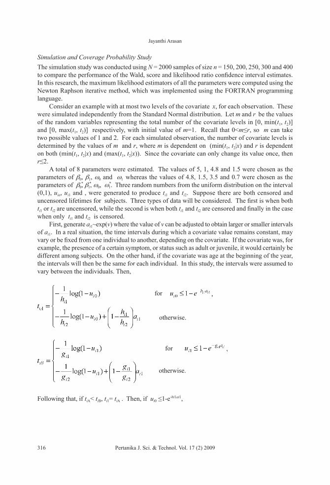
Simulation and Coverage Probability StudyThe simulation study was conducted using N = 2000 samples of size n = 150, 200, 250, 300 and 400 to compare the performance of the Wald, score and likelihood ratio confidence interval estimates. In this research, the maximum likelihood estimators of all the parameters were computed using the Newton Raphson iterative method, which was implemented using the FORTRAN programming language. Consider an example with at most two levels of the covariate x, for each observation. These were simulated independently from the Standard Normal distribution. Let m and r be the values of the random variables representing the total number of the covariate levels in [0, min(t1, t2)] and [0, max(t1, t2)] respectively, with initial value of m=1. Recall that 0<m≤r, so m can take two possible values of 1 and 2. For each simulated observation, the number of covariate levels is determined by the values of m and r, where m is dependent on (min(t1, t2|x) and r is dependent on both (min(t1, t2|x) and (max(t1, t2|x)). Since the covariate can only change its value once, then r≤2. A total of 8 parameters were estimated. The values of 5, 1, 4.8 and 1.5 were chosen as the parameters of b0, b1, w0 and w1 whereas the values of 4.8, 1.5, 3.5 and 0.7 were chosen as the parameters of b0, b1, w0, w1. Three random numbers from the uniform distribution on the interval (0,1), uio, ui1 and , were generated to produce ti1 and ti2. Suppose there are both censored and uncensored lifetimes for subjects. Three types of data will be considered. The first is when both ti1 or ti2 are uncensored, while the second is when both ti1 and ti2 are censored and finally in the case when only ti1 and ti2 is censored. First, generate ai1~exp(v) where the value of v can be adjusted to obtain larger or smaller intervals of ai1. In a real situation, the time intervals during which a covariate value remains constant, may vary or be fixed from one individual to another, depending on the covariate. If the covariate was, for example, the presence of a certain symptom, or status such as adult or juvenile, it would certainly be different among subjects. On the other hand, if the covariate was age at the beginning of the year, the intervals will then be the same for each individual. In this study, the intervals were assumed to vary between the individuals. Then,

Following that, if tiA< tiB, ti1= tiA . Then, if ui0 ≤1-e-hi1ai1,

* **

otherwise.

otherwise.

for

for



If ui0 >1-e-hi1ai1, . Otherwise if tiB < tiA, ti2 = tiB. Then, if ui1 ≤1-e-gi1ai1

If

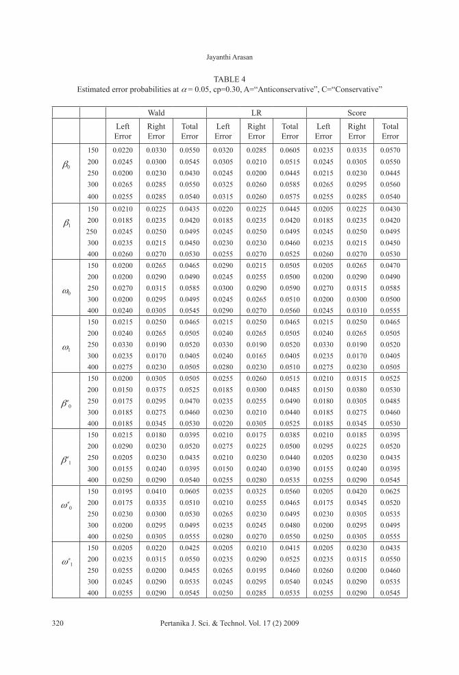
The censoring time, ci~exp(μ), where the value of μ would be adjusted to obtain the desired approximate censoring proportion in the data of the present study. In this research, the two levels of approximate censoring proportions, cp=0.10 and cp=0.30, were used to see how they affected the performance of the interval estimates. The values of cp=0.10 and cp=0.30 were chosen to represent both low and high levels of censoring proportions, respectively. The coverage probability is the probability that an interval contains the true parameter value. The study was conducted by calculating the left and right estimated error probabilities for each of the parameter estimates. The estimated left (right) error probability was calculated by adding the number of times the left (right) endpoint was more (less) than the true parameter value, divided by the total number of samples, N. Following Doganaksoy and Schmee (1993), if the total error probability is greater than α + 2.58 s.e (at ), the method is then termed as anticonservative, and if it is lower than α-2.58 s.e (at ), the method is termed as conservative. The estimated error probabilities are known as symmetric when the larger error probability is less than 1.5 times the smaller one.

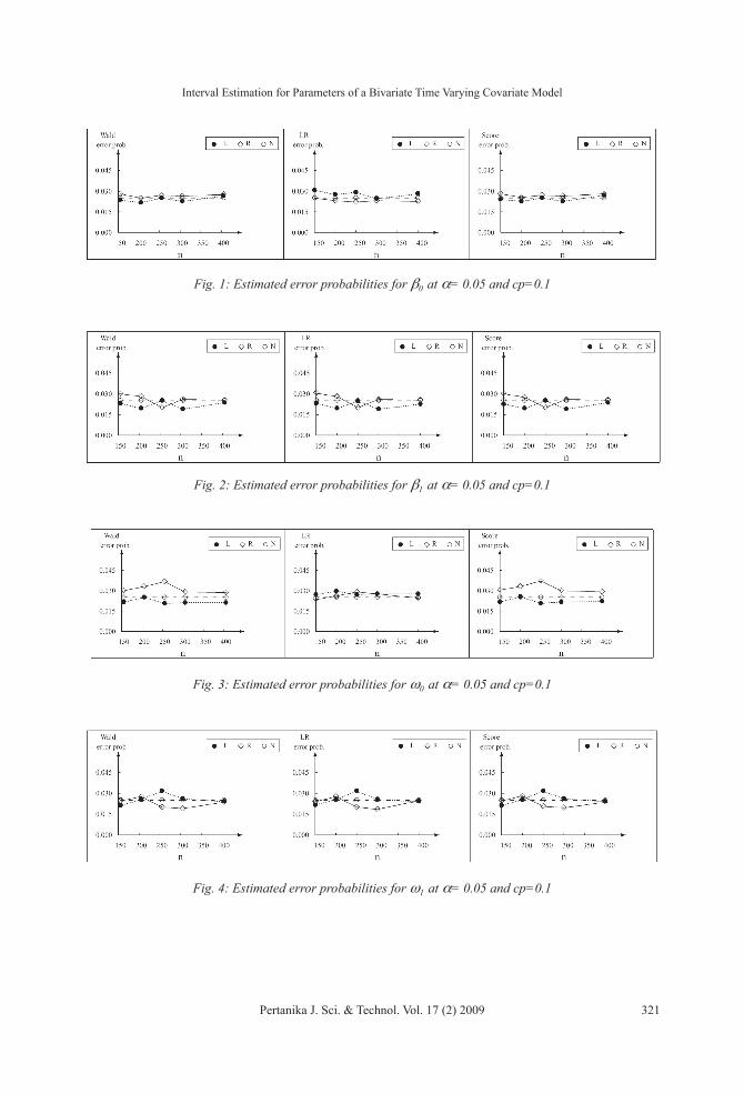
RESULTS AND DISCUSSIONThe summary of the simulation results, comparing the performances of the Wald, LR and score intervals, is given in Tables 1 and 2. These tables display the total number of anticonservative, conservative and asymmetrical intervals, generated by each of these methods at different nominal error probabilities, and censoring proportion. Tables 3 and 4 provide some of the more detailed results and show how the intervals performed at different sample sizes. Figs. 1 through 4 give a graphical view of some of the coverage probabilities for each of the methods when α= 0.05 and cp=10%. Tables 1 and 2 show that all the intervals produced 1 anticonservative and 2 conservative intervals, but only when the nominal level, α is high. The LR method clearly generates intervals which are more symmetrical than the other two methods. It only produced 1 asymmetrical interval when the censoring proportion in the data is low

for

otherwise.

otherwise.

for

Jayanthi Arasan


TABLE 1Summary of the number of interval estimates at α = 0.05

Cp=0.10 Cp=0.30Type of interval

Wald LR Score Wald LR Score

Anticonservative(A) 0 0 0 0 0 0Conservative(C) 0 0 0 0 0 0Asymetrical 9 1 9 9 3 9

TABLE 2Summary of the number of interval estimates at α = 0.10

Cp=0.10 Cp=0.30Type of interval

Wald LR Score Wald LR Score

Anticonservative(A) 1 1 1 0 0 0

Conservative(C) 1 1 1 1 1 1

Asymetrical 6 1 5 4 0 4

and α is 0.05, whereas the Wald and score generated 9 asymmetrical intervals. The high censoring level in the data seems to affect the LR more than the other methods, but only when α is low where it starts to produce more asymmetrical intervals. However, this number is still much lower than the number of asymmetrical intervals generated by the Wald and score intervals. Both Wald and score methods gave almost similar results, but the score method appears to be slightly more symmetrical than the Wald. However, the Wald has more intervals with the total error probability closer to the nominal level than the score intervals. The increase in the censoring proportion does not seem to affect the performances of the Wald and score intervals. When both α and censoring proportion is high, the performances of all the intervals seem to be slightly improved, where they produce fewer asymmetrical intervals, particularly the LR interval. The reason for this is probably the highly censored data that generates wider intervals because of the larger standard errors of the parameter estimates. This produces more intervals that include the true parameter value. All the methods seem to generate more conservative and anticonservative intervals, but fewer asymmetrical intervals when α is high. They also seem to converge to the nominal level at almost the same rate, but the LR intervals perform slightly better than the other two when the size of the sample is lower.

CONCLUSIONSOverall, the LR method appears to perform best since it has the least number of asymmetrical intervals. It should be the preferred method, specifically when the censoring level in the data is low. Although the high censoring level and low value of α seem to affect the LR in that it produces more asymmetrical intervals, the number of these asymmetrical intervals are still relatively low. Similarly, the LR intervals are still more symmetrical than the intervals produced by the other two methods.



\

Wald LR Score

Left Error

Right Error

Total Error

Left Error

Right Error

Total Error

Left Error

Right Error Total Error

150 0.0235 0.0280 0.0515 0.0305 0.0250 0.0555 0.0240 0.0280 0.0520

b0 200 0.0215 0.0250 0.0465 0.0275 0.0230 0.0505 0.0225 0.0255 0.0480

250 0.0250 0.0270 0.0520 0.0290 0.0220 0.0510 0.0250 0.0270 0.0520

300 0.0225 0.0265 0.0490 0.0245 0.0230 0.0475 0.0225 0.0265 0.0490

400 0.0265 0.0275 0.0540 0.0280 0.0225 0.0505 0.0270 0.0280 0.0550

150 0.0230 0.0300 0.0530 0.0230 0.0305 0.0535 0.0225 0.0300 0.0525

200 0.0195 0.0280 0.0475 0.0195 0.0280 0.0475 0.0195 0.0275 0.0470

b1 250 0.0250 0.0200 0.0450 0.0245 0.0200 0.0445 0.0250 0.0200 0.0450

300 0.0190 0.0260 0.0450 0.0190 0.0260 0.0450 0.0190 0.0260 0.0450

400 0.0235 0.0255 0.0490 0.0225 0.0255 0.0480 0.0235 0.0255 0.0490

150 0.0215 0.0300 0.0515 0.0270 0.0235 0.0505 0.0215 0.0305 0.0520

200 0.0250 0.0330 0.0580 0.0295 0.0260 0.0555 0.0255 0.0330 0.0585

w0250 0.0205 0.0365 0.0570 0.0270 0.0290 0.0560 0.0205 0.0370 0.0575

300 0.0210 0.0290 0.0500 0.0275 0.0275 0.0550 0.0215 0.0300 0.0515

400 0.0210 0.0285 0.0495 0.0275 0.0245 0.0520 0.0220 0.0290 0.0510

150 0.0210 0.0245 0.0455 0.0215 0.0240 0.0455 0.0210 0.0245 0.0455

200 0.0255 0.0275 0.0530 0.0255 0.0275 0.0530 0.0255 0.0280 0.0535

w1250 0.0315 0.0200 0.0515 0.0315 0.0200 0.0515 0.0315 0.0205 0.0520

300 0.0260 0.0190 0.0450 0.0255 0.0185 0.0440 0.0260 0.0195 0.0455

400 0.0240 0.0235 0.0475 0.0240 0.0245 0.0485 0.0240 0.0235 0.0475

150 0.0210 0.0335 0.0545 0.0295 0.0285 0.0580 0.0215 0.0340 0.0555

200 0.0170 0.0360 0.0530 0.0225 0.0300 0.0525 0.0170 0.0365 0.0535

b0* 250 0.0155 0.0295 0.0450 0.0180 0.0250 0.0430 0.0160 0.0305 0.0465

300 0.0190 0.0250 0.0440 0.0225 0.0240 0.0465 0.0190 0.0250 0.0440400 0.0180 0.0300 0.0480 0.0200 0.0255 0.0455 0.0190 0.0310 0.0500150 0.0225 0.0240 0.0465 0.0245 0.0255 0.0500 0.0235 0.0240 0.0475200 0.0305 0.0275 0.0580 0.0305 0.0265 0.0570 0.0305 0.0275 0.0580

b1* 250 0.0205 0.0225 0.0430 0.0210 0.0225 0.0435 0.0205 0.0225 0.0430

300 0.0170 0.0230 0.0400 0.0170 0.0235 0.0405 0.0170 0.0230 0.0400400 0.0205 0.0300 0.0505 0.0205 0.0300 0.0505 0.0205 0.0305 0.0510150 0.0195 0.0370 0.0565 0.0235 0.0310 0.0545 0.0195 0.0380 0.0575200 0.0185 0.0340 0.0525 0.0205 0.0265 0.0470 0.0185 0.0345 0.0530

w*0

250 0.0185 0.0345 0.0530 0.0215 0.0295 0.0510 0.0185 0.0350 0.0535300 0.0280 0.0305 0.0585 0.0310 0.0265 0.0575 0.0280 0.0315 0.0595

400 0.0255 0.0335 0.0590 0.0290 0.0285 0.0575 0.0255 0.0335 0.0590

150 0.0255 0.0315 0.0570 0.0245 0.0310 0.0555 0.0250 0.0315 0.0565

200 0.0235 0.0275 0.0510 0.0240 0.0280 0.0520 0.0240 0.0280 0.0520

w*0 250 0.0285 0.0215 0.0500 0.0280 0.0215 0.0495 0.0285 0.0215 0.0500

300 0.0290 0.0235 0.0525 0.0290 0.0240 0.0530 0.0290 0.0235 0.0525

400 0.0255 0.0325 0.0580 0.0255 0.0325 0.0580 0.0255 0.0325 0.0580

TABLE 3Estimated error probabilities at α = 0.05, cp=0.10, A=“Anticonservative”, C=“Conservative”

Jayanthi Arasan


TABLE 4Estimated error probabilities at α = 0.05, cp=0.30, A=“Anticonservative”, C=“Conservative”

Wald LR Score

Left Error

Right Error

Total Error

Left Error

Right Error

Total Error

Left Error

Right Error

Total Error

150 0.0220 0.0330 0.0550 0.0320 0.0285 0.0605 0.0235 0.0335 0.0570

b0 200 0.0245 0.0300 0.0545 0.0305 0.0210 0.0515 0.0245 0.0305 0.0550

250 0.0200 0.0230 0.0430 0.0245 0.0200 0.0445 0.0215 0.0230 0.0445

300 0.0265 0.0285 0.0550 0.0325 0.0260 0.0585 0.0265 0.0295 0.0560

400 0.0255 0.0285 0.0540 0.0315 0.0260 0.0575 0.0255 0.0285 0.0540

150 0.0210 0.0225 0.0435 0.0220 0.0225 0.0445 0.0205 0.0225 0.0430

b1200 0.0185 0.0235 0.0420 0.0185 0.0235 0.0420 0.0185 0.0235 0.0420

250 0.0245 0.0250 0.0495 0.0245 0.0250 0.0495 0.0245 0.0250 0.0495

300 0.0235 0.0215 0.0450 0.0230 0.0230 0.0460 0.0235 0.0215 0.0450

400 0.0260 0.0270 0.0530 0.0255 0.0270 0.0525 0.0260 0.0270 0.0530

150 0.0200 0.0265 0.0465 0.0290 0.0215 0.0505 0.0205 0.0265 0.0470

200 0.0200 0.0290 0.0490 0.0245 0.0255 0.0500 0.0200 0.0290 0.0490

w0 250 0.0270 0.0315 0.0585 0.0300 0.0290 0.0590 0.0270 0.0315 0.0585

300 0.0200 0.0295 0.0495 0.0245 0.0265 0.0510 0.0200 0.0300 0.0500

400 0.0240 0.0305 0.0545 0.0290 0.0270 0.0560 0.0245 0.0310 0.0555

150 0.0215 0.0250 0.0465 0.0215 0.0250 0.0465 0.0215 0.0250 0.0465

200 0.0240 0.0265 0.0505 0.0240 0.0265 0.0505 0.0240 0.0265 0.0505

w1 250 0.0330 0.0190 0.0520 0.0330 0.0190 0.0520 0.0330 0.0190 0.0520

300 0.0235 0.0170 0.0405 0.0240 0.0165 0.0405 0.0235 0.0170 0.0405

400 0.0275 0.0230 0.0505 0.0280 0.0230 0.0510 0.0275 0.0230 0.0505

150 0.0200 0.0305 0.0505 0.0255 0.0260 0.0515 0.0210 0.0315 0.0525

200 0.0150 0.0375 0.0525 0.0185 0.0300 0.0485 0.0150 0.0380 0.0530

b*0

250 0.0175 0.0295 0.0470 0.0235 0.0255 0.0490 0.0180 0.0305 0.0485300 0.0185 0.0275 0.0460 0.0230 0.0210 0.0440 0.0185 0.0275 0.0460400 0.0185 0.0345 0.0530 0.0220 0.0305 0.0525 0.0185 0.0345 0.0530150 0.0215 0.0180 0.0395 0.0210 0.0175 0.0385 0.0210 0.0185 0.0395200 0.0290 0.0230 0.0520 0.0275 0.0225 0.0500 0.0295 0.0225 0.0520

b*1

250 0.0205 0.0230 0.0435 0.0210 0.0230 0.0440 0.0205 0.0230 0.0435300 0.0155 0.0240 0.0395 0.0150 0.0240 0.0390 0.0155 0.0240 0.0395400 0.0250 0.0290 0.0540 0.0255 0.0280 0.0535 0.0255 0.0290 0.0545150 0.0195 0.0410 0.0605 0.0235 0.0325 0.0560 0.0205 0.0420 0.0625

w*0

200 0.0175 0.0335 0.0510 0.0210 0.0255 0.0465 0.0175 0.0345 0.0520250 0.0230 0.0300 0.0530 0.0265 0.0230 0.0495 0.0230 0.0305 0.0535300 0.0200 0.0295 0.0495 0.0235 0.0245 0.0480 0.0200 0.0295 0.0495

400 0.0250 0.0305 0.0555 0.0280 0.0270 0.0550 0.0250 0.0305 0.0555

150 0.0205 0.0220 0.0425 0.0205 0.0210 0.0415 0.0205 0.0230 0.0435

w*1

200 0.0235 0.0315 0.0550 0.0235 0.0290 0.0525 0.0235 0.0315 0.0550

250 0.0255 0.0200 0.0455 0.0265 0.0195 0.0460 0.0260 0.0200 0.0460

300 0.0245 0.0290 0.0535 0.0245 0.0295 0.0540 0.0245 0.0290 0.0535

400 0.0255 0.0290 0.0545 0.0250 0.0285 0.0535 0.0255 0.0290 0.0545



Fig. 1: Estimated error probabilities for b0 at α= 0.05 and cp=0.1

Fig. 2: Estimated error probabilities for b1 at α= 0.05 and cp=0.1

Fig. 3: Estimated error probabilities for w0 at α= 0.05 and cp=0.1

Fig. 4: Estimated error probabilities for w1 at α= 0.05 and cp=0.1

Jayanthi Arasan


Thus, the Wald method can be considered when both α and the censoring proportion are high, or when a simpler and faster method is required. It is probably not advisable to consider applying the Wald intervals in other settings because it generally generates the most number of asymmetrical intervals. The score method may perform as good as the Wald, but it involves a lot of computational effort. Thus, this method should not be considered, unless as a measure of comparison. These findings are consistent with the results of Doganaksoy and Schmee (1993) who found the Wald intervals to be highly asymmetrical as compared to the LR, when dealing with censored data. However, the LR method involves a great deal of computational effort, which may not actually justify its improved performance when compared to the much more straightforward Wald method. The discussion on the model involving time varying covariates has been restricted to two intervals, during which the covariates value remains constant. It would be possible to carry out further work to include models involving more intervals and this could be programmed relatively easily. The model can also be extended to consider the case, in which the components have the Weibull lifetime distribution.

REFERENCESBarndorff-Nielsen, O.E. and Cox, D.R. (1984). Bartlett adjustments to the likelihood ratio statistic and the

distribution of the maximum likelihood estimator. Journal of Royal Statistical Society, B(46), 483–495.

Beck, N. (1999). Modelling Space and Time: The Event History Approach. In S. Elinor and T. Eric (Eds.), Research Strategies in the Social Sciences: A Guide to New Approaches. Oxford: Oxford University Press.

Bennet, D.S. (1999). Parametric models, duration dependence and time-varying data revisited. American Journal of Political Science, 43, 256–270.

Blossfield, Hans-Peter, Hamerle, A. and Mayer, K.U. (1989). Event History Analysis. Hillsdale, New Jersey: Lawrence Erlbaum Associates.

Box-Steffensmeier, J.M. and Jones, B.S. (1997). Time is of the essence: Event history models in political science. American Journal of Political Science, 41, 1414–1461.

Courgeau, D. and Lelièvre, E. (1992). Event History Analysis in Demography. Oxford: Clarendon Press.

Cox, D.R. and Hinkley, D.V. (1979). Theoretical Statistics. New York: Chapman and Hall.

Diciccio, T.J. (1988). Approximate inference for generalised gamma distribution. Technometrics, 29, 33–40.

Doganaksoy, N. and Schmee, J. (1993a). Comparison of approximate confidence intervals for distributions used in life-data analysis. Technometrics, 35(2), 175–184.

Doganaksoy, N. and Schmee, J. (1993b). Comparison of approximate confidence intervals for smallest extreme value distribution simple linear regression model under time censoring. Communications in Statistics-Simulation and Computation, 2, 175–184.

Freund, J.E. (1961). A bivariate extension of the exponential distribution. Journal of American Statistical Association, 56, 971–977.

Jeng, S.L. and Meeker, W.Q. (2000). Comparison for approximate confidence interval procedure for type I censored data. Technometrics, 42(2), 135–148.

Kalbfleisch, J.D. and Prentice, R.L. (1980). The Statistical Analysis of Failure Time Data. New York: Wiley.

Lawless, J.F. (1982). Statistical Models and Methods for Lifetime Data. New York: Wiley.



Nelson, W. (1990). Accelerated Testing: Statistical Models, Test Plans, and Data Analysis. New York: Wiley.

Ostrouchov, G. and Meeker, W.Q. (1988). Accuracy of approximate confidence bounds computed from interval censored Weibull and lognormal data. Journal of Statistical Computation and Simulation, 29, 43–76.

Petersen, T. (1986). Fitting parametric survival models with time-dependent covariates. Journal of Applied Statistics, 35(3), 281–288.

Rao, C.R. (n.d.). Large sample tests of statistical hypotheses concerning several parameters with applications to problems of estimation. Proceedings of the Cambridge Philosophical Society, 44, 50-57, 1948.

Tuma, B.N. and Hannan, M.T. (1984). Social Dynamics: Models and Methods. Orlando, Florida: Academic Press.

Yamaguchi, K. (1991). Event History Analysis. New York: Sage Publications.

Venzon, D.J. and Moolgavkar, S.H. (1988). A method for computing profile-likelihood-based confidence intervals. Applied Statistics, 37, 87–94.

interval estimation for parameters of a bivariate time ... papers/jst vol. 17 (2) jul....

Documents