Interpreting Spectral Energy Distributions from Young Stellar

Objects. I. A grid of 200,000 YSO model SEDs.

Thomas P. Robitaille1

Barbara A. Whitney2

Remy Indebetouw3

Kenneth Wood1

Pia Denzmore4

ABSTRACT

We present a grid of radiation transfer models of axisymmetric young stellar

objects (YSOs), covering a wide range of stellar masses (from 0.1M� to 50M�)

and evolutionary stages (from the early envelope infall stage to the late disk-only

stage). The grid consists of 20,000 YSO models, with spectral energy distribu-

tions (SEDs) and polarization spectra computed at ten viewing angles for each

model, resulting in a total of 200,000 SEDs. We made a careful assessment of the

theoretical and observational constraints on the physical conditions of disks and

envelopes in YSOs, and have attempted to fully span the corresponding regions

in parameter space. These models are publicly available on a dedicated WWW

server 1. In this paper we summarize the main features of our models, as well as

the range of parameters explored. Having a large grid covering reasonable regions

of parameter space allows us to shed light on many trends in near- and mid-IR

observations of YSOs (such as changes in the spectral indices and colors of their

SEDs), linking them with physical parameters (such as disk and infalling envelope

parameters). In particular we examine the dependence of the spectral indices of

1SUPA, School of Physics and Astronomy, University of St Andrews, North Haugh, St Andrews, KY169SS, United Kingdom; tr9@st-andrews.ac.uk, kw25@st-andrews.ac.uk

2Space Science Institute, 4750 Walnut St. Suite 205, Boulder, CO 80301, USA; bwhitney@spacescience.org

3University of Virginia, Astronomy Dept., P.O. Box 3818, Charlottesville, VA, 22903-0818; re-my@virginia.edu

4Physics and Astronomy Department, Rice University, Houston, TX, USA; piadenz@rice.edu

1http://www.astro.wisc.edu/protostars

– 2 –

the model SEDs on envelope accretion rate and disk mass. In addition, we show

variations of spectral indices with stellar temperature, disk inner radius, and disk

flaring power for a subset of disk-only models. We also examine how changing the

wavelength range of data used to calculate spectral indices affects their values.

We show sample color-color plots of the entire grid as well as simulated clusters

at various distances with typical Spitzer Space Telescope sensitivities. We find

that young embedded sources generally occupy a large region of color-color space

due to inclination and stellar temperature effects. Disk sources occupy a smaller

region of color-color space, but overlap substantially with the region occupied

by embedded sources, especially in the near- and mid-IR. We identify regions in

color-color space where our models indicate that only sources at a given evolu-

tionary stage should lie. We find that while near-IR (such as JHK) and mid-IR

(such as IRAC) fluxes are useful in discriminating between stars and YSOs, and

are useful for identifying very young sources, the addition of longer wavelength

data such as MIPS 24µm is extremely valuable for determining the evolutionary

stage of YSOs.

Subject headings: astronomical data bases: miscellaneous — circumstellar matter

— infrared: stars — radiative transfer — stars: formation — stars: pre-main-

sequence — polarization

1. Introduction

An explosion of infrared data on star formation regions is being collected by the Spitzer

Space Telescope and will continue to be collected by future missions such as the Herschel

Space Observatory and the James Webb Space Telescope. Despite its modest size (0.85 m),

the Spitzer Space Telescope is much more sensitive and has higher spatial resolution than

previous infrared observatories (Werner et al. 2004). It is also very efficient, and has mapped

a substantial fraction of the star formation regions in the Galaxy using the IRAC (3.6,

4.5, 5.8, and 8µm; Fazio et al. 2004) and MIPS (24, 70, and 160µm; Rieke et al. 2004)

instruments. For example, the GLIMPSE (Benjamin et al. 2003) and MIPSGAL (PI Carey)

Legacy surveys are mapping over 150 square degrees of the inner Galactic plane; the Cores-

to-Disks (c2d) Legacy project has surveyed five nearby large molecular clouds (Evans et al.

2003); and several projects are surveying the Orion molecular cloud (Megeath et al. 2005a),

the Taurus molecular cloud (Hartmann et al. 2005), the LMC (Chu et al. 2005; Meixner et al.

2006) and SMC, and many other well-known star formation regions (e.g Gutermuth et al.

2004; Megeath et al. 2005b; Allen et al. 2006; Sicilia-Aguilar et al. 2006). These data can

– 3 –

be combined with other surveys, such as the 2MASS near-infrared all-sky survey (Skrutskie

et al. 2006), expanding the wavelength coverage of the observed YSOs.

Our particular goal is to characterize YSOs in the Galaxy using the GLIMPSE and

MIPSGAL surveys, as well as in the LMC using the SAGE survey, and to determine the

timescales of various evolutionary stages as a function of stellar mass and location in the

Galaxy. Ultimately, we hope to provide an independent estimate of the star formation rate

and efficiency in the Galaxy and the LMC.

To help analyze the SEDs of YSOs we developed radiation transfer models (Whitney

et al. 2003a,b, 2004). The well-known classification for low-mass YSOs uses the spectral

index α (the slope of log10 λFλ vs log10 λ longward of 2µm) to classify a source as embedded

(α > 0; Class I), a disk source (−2 < α < 0; Class II) or a source with an optically thin or

no disk (α < −2; Class III) (Lada 1987). However, our models indicate that the spectral

index and the colors of a YSO in certain wavelength ranges are not always directly related to

its evolutionary stage. For example, an edge-on embedded protostar can have a decreasing

slope in the narrow wavelength range of 2−10µm if the flux is dominated by scattered light

(edge-on disks exhibit similar behavior, Wood et al. 2002b, Grosso et al. 2003). In addition,

the temperature of the central source also affects the colors in this wavelength range, as does

the location of the inner radius of the disk: hot stellar sources and large inner disk holes can

produce red colors in a star+disk source (see Section 3.4).

In an attempt to improve our physical understanding gained from interpreting the SEDs

of the many sources found in these surveys, many of which only have JHK, IRAC, and MIPS

24µm data, we plan to fit observed SEDs using a large grid of pre-computed model SEDs.

This grid attempts to encompass a large range of stellar masses and YSO evolutionary stages.

We sampled the model parameters based on both theory and observations (see Section 2.2).

This paper describes our publicly available grid of models. A companion paper (Robitaille

et al. 2006, in preparation) describes the method used to fit observed SEDs using the

grid of models. The advantages of fitting pre-computed SEDs to data, even in the fairly

narrow wavelength range mentioned above, are that 1) one makes use of all available data

simultaneously without loss of information 2) the uniqueness or non-uniqueness of a fit is

immediately apparent from the range of model parameters that can fit a given SED, and 3)

it is an efficient technique when used with large datasets as the model SEDs do not have to

be computed for each source. In Section 2 we describe the grid of models. Section 3 shows

results from the grid, including sample SEDs, polarization spectra, and color-color plots, as

well as an analysis of spectral index and color-color plot classifications. Finally, in Section 4

we make concluding remarks.

– 4 –

2. The grid of models

2.1. The radiation transfer code

2.1.1. Brief description of the code

The Monte Carlo radiation transfer code used for this grid of models includes non-

isotropic scattering, polarization, and thermal emission from dust in a spherical-polar grid,

solving for the temperature using the method of Bjorkman & Wood (2001). This code is

publicly available 2. The circumstellar geometry consists of a rotationally-flattened infalling

envelope (Ulrich 1976; Terebey et al. 1984), bipolar cavities (Whitney & Hartmann 1993;

Whitney et al. 2003a) and a flared accretion disk (Shakura & Sunyaev 1973; Pringle 1981;

Kenyon & Hartmann 1987; Chiang & Goldreich 1997; D’Alessio et al. 1998; Dullemond et al.

2001). The luminosity sources include the central star and disk accretion. The code and the

model geometries are described in detail in Whitney et al. (2003a,b).

As discussed in Section 2.2, the various model parameters are sampled in order to

produce a range of evolutionary stages. For example, the envelope accretion rate decreases

over time, the bipolar cavities become wider, the dust in the cavities less dense, and the disk

radius increases during the early accretion from the envelope.

2.1.2. Dust grain models

Our grain models contain a mixture of astronomical silicates and graphite in solar abun-

dance, using the optical constants of Laor & Draine (1993). The optical properties are av-

eraged over the size distribution and composition. Thus we do not separate the heating and

emission properties of different grain sizes or composition. This could affect the thermal and

chemical properties in the inner regions of the disk (Wolf 2003) but its affect on the SED is

expected to be relatively minor (Wolf 2003; Carciofi et al. 2004).

The grain properties vary with location in the disk and envelope as follows: the densest

regions of the disk (nH2 > 1010 cm−3) use a grain model with a size distribution that decays

exponentially for sizes larger than 50µm and extends up to 1 mm; this grain model fits the

SED of the HH30 disk (Wood et al. 2002b). This is the same as the “Disk midplane” grain

model described in Table 3 of Whitney et al. (2003a). The rest of the circumstellar geometry

uses a grain size distribution with an average particle size slightly larger than the diffuse

2http://www.astro.wisc.edu/protostars

– 5 –

ISM, and a ratio of total-to-selective extinction RV = 3.6. This is the “KMH” model (Kim,

Martin, & Hendry 1994), referred to as the “Outflow” model in Table 3 of Whitney et al.

(2003a). Dust grains in embedded regions of Taurus show evidence for further grain growth,

with RV ∼ 4 in the densest regions (Whittet et al. 2001), but recent models of near-IR

images of Taurus protostars show that larger grain models are not well-distinguished from

ISM grains (Wolf & Hillenbrand 2003; Stark et al. 2006; Gramajo et al. 2006). Grains in

molecular clouds also show evidence for ice coatings (e.g. Boogert & Ehrenfreund 2004; Knez

et al. 2005), which are not included in our models.

2.1.3. Stellar photospheres

The spectrum of the central source for each model is dependent mainly on its tempera-

ture and to a lesser extent its surface gravity. For stellar temperatures below 10, 000 K, we

used model stellar photospheres from Brott & Hauschildt (2005), while for stellar tempera-

tures above 10, 000 K we used model stellar photospheres from Kurucz (1993). In both cases

we assumed solar metallicity. For each YSO model, we interpolated the stellar photospheres

to the relevant temperature and surface gravity.

2.1.4. Model parameters

Technically speaking the set of models we present in this paper does not form a ‘grid’,

since the parameters are randomly sampled within ranges. However, we will refer to the set

of models as a ‘model grid’, since this is a useful descriptive term.

The 14 model parameters are shown in Table 1. Fortunately, only a few parameters

are important at a given evolutionary stage. For example in the youngest stages, the disk

is hidden beneath the envelope: the disk inner radius, accretion rate, and to a lesser extent

disk mass are the main disk parameters that affect the 1-8µm fluxes. The presence of an

inner disk is required to produce mid-IR flux and to obscure the central source at edge-on

viewing angles, but the dust properties in the disk and the amount of flaring do not have an

important effect on the mid-IR SED. At these young stages, the most important parameters

are the envelope accretion rate, the opening angle of the bipolar cavities, the inclination

to the line of sight, the disk/envelope inner radius, the stellar temperature, and to a lesser

extent the disk mass. At later stages, when the envelope has mostly dispersed, the most

relevant parameters for the SED are the disk inner radius, accretion rate, mass, and flaring

(or dust settling) (Kenyon & Hartmann 1987; Lada & Adams 1992; Chiang & Goldreich

– 6 –

1997; D’Alessio et al. 1998; Furlan et al. 2005).

The details of the parameter sampling are given in Section 2.2. It is important to note

at this point that we are not suggesting our own model of evolution for YSOs. Instead, our

aim is to provide model SEDs for stages of evolution that have been suggested by theory or

observations. Furthermore, we do not follow several objects throughout their evolution, but

instead we sample possible evolutionary stages and stellar masses randomly.

2.1.5. Output of the radiation transfer code

The output from the code presented here consists of flux and polarization spectra for 250

wavelengths (from 0.01 to 5, 000µm), computed at 10 viewing angles (from pole-on to edge-

on in equal intervals of cosine of the inclination) and in 50 different circular apertures (with

radii from 100 to 100, 000 AU). Since each one of the 20,000 models produces an SED (flux

vs. wavelength) for each viewing angle and aperture, our grid of models contains 10 million

SEDs. The code can produce images at specific viewing angles, but we did not compute

these in the current grid as doing so would increase the CPU time required. However, the

50 apertures from 100 − 100, 000 AU amount to a spherically averaged intensity profile for

each viewing angle of each model.

We have convolved all our models with a large number of common filter bandpasses

ranging from optical to sub-mm wavelengths, including for example optical (e.g. UBVRI),

near-IR (e.g. 2MASS JHK), mid- and far-IR (e.g. IRAC, MSX, IRAS, MIPS), and sub-mm

(e.g. Scuba 450 and 850µm) filters. We will expand the range of filters used to convolve the

SEDs as requested by users. The polarization spectra have a lower signal-to-noise than the

SEDs, so we smooth them before convolving with broadband filter profiles.

For the grid of models presented here, we ran each model with 20,000,000 ‘photons’

(energy packets, Bjorkman & Wood 2001). This produces SEDs with good signal-to-noise

ratios for wavelengths spanning 1 − 100µm (however, we note that the signal-to noise may

also be good outside this range). The wavelength range at which a model SED has a

good signal-to-noise depends on the evolutionary stage of the YSO: SEDs may be noisy at

wavelengths shorter than 1µm , but with a good signal-to noise at sub-mm wavelengths for

young embedded sources, or be noisy and at wavelengths longer than about 100µm and with

a good signal-to-noise at optical and near-UV wavelengths for low mass disks. Figure 1 shows

the median noise levels as a function of wavelength (using the SEDs measured in the largest

aperture). We provide estimated uncertainties on our SEDs so that they are still usable

in most wavelength ranges. The SEDs can be re-binned to a lower wavelength resolution

– 7 –

to reduce these uncertainties. Future versions of the grid will include higher signal-to-noise

SEDs as well as images.

The time taken for each model to run varies with optical depth and covering factor of

circumstellar material as seen from the radiation source. A disk model typically takes an

hour to run on a 3 GHz Intel processor, and an embedded protostar can take 10 hours. The

total CPU time for the entire model grid, which was run on three different clusters, was

approximately 65,000 hours (or roughly three weeks using approximately 60 CPUs).

The grid of models is available on a dedicated web server 3. This includes SEDs and

polarization spectra for each inclination and aperture of each model. Various components of

the SED can be viewed separately, such as the flux emitted by the disk, star, or envelope, the

scattered flux, and the direct stellar flux, as described in Section 3.2. Fluxes and magnitudes

for common filter functions are also available.

2.2. Sampling of the model parameters

In the following section we present a detailed description of the parameter sampling. It

is not possible to explore parameter space in its entirety in a completely unbiased manner.

Therefore we have had to make arbitrary decisions concerning the ranges of parameter values.

The parameter ranges covered by the grid of models span those determined from observations

and theories, and can be divided into three categories: the central source parameters (stellar

mass, radius and temperature), the infalling envelope parameters (the envelope accretion

rate, outer radius, inner radius, cavity opening angle and cavity density), and the disk

parameters (disk mass, outer radius, inner radius, flaring power, and scaleheight). Also

included is a parameter describing the ambient density surrounding the YSO.

All the masses, mass accretion rates and densities for the disk and envelope parameters

assume a gas-to-dust ratio of 100. Note that the results can be scaled to different gas-to-dust

ratios since only the dust is taken into account in the radiation transfer. For example, a

disk with a total mass of 0.01M� in a region where the gas-to-dust ratio is 100 will produce

the same SED as a disk with a total mass of 0.1M� in a region where the gas-to-dust ratio

is 1000 (such as a low-metallicity galaxy or perhaps the outer Milky Way). In addition to

disk masses, the following parameter values should be rescaled accordingly in regions where

the gas-to-dust ratio is not 100: the envelope accretion rates, disk accretion rates, cavity

densities and ambient densities. Note that it is only necessary to re-scale the parameter

3http://www.astro.wisc.edu/protostars

– 8 –

values, and that it is not necessary to re-run the radiation transfer models

2.2.1. The Stellar Parameters

The parameters for the 20,000 YSO models were chosen using the following procedure.

First a stellar mass M� was randomly sampled from the following probability distribution

function:

f(M�)dM� =1

loge 10

1

log10 M2 − log10 M1

dM�

M�(1)

The masses were sampled between M1 = 0.1M� and M2 = 50M�. This produced a

constant density of models in log10 M� space. Following this, a random stellar age t� was

sampled from a similar probability distribution function:

f(t�)dt� =1

6

1

t1/6max − t

1/6min

dt�

t5/6�

(2)

The ages were sampled between tmin = 103 yr and tmax = 107 yr. This distribution

produced a density of models close to constant in log10 t� space, but with a slight bias towards

larger values of t�. This was done to avoid a deficit of disk-only models. In cases where the

resulting values of the stellar age were greater than the combined pre-main sequence and

main-sequence lifetime of the star (estimated from the sampled masses M�), the age was

resampled until it was within the adequate lifetime. The values of M� and t� for the 20,000

models are shown in Figure 2.

For each set of M� and t� the values of the stellar radius R� and temperature T� were

found by interpolating pre-main sequence evolutionary tracks (Bernasconi & Maeder 1996 for

M� ≥ 9M�; Siess et al. 2000 for M� ≤ 7M�; a combination of both for 7M� < M� < 9M�).

The values of T� and R� are shown in Figure 3. It is important to note that the evolutionary

age of the central sources is not a parameter in the radiation transfer code, and was only

used to get a coherent radius and temperature as well as approximate ranges of disk and

envelope parameters. Any errors in the evolutionary tracks can easily be accommodated by

the large range of parameter values allowed at a given age. Furthermore it is always possible

to reassign a stellar source age to a model if it is found that a different set of evolutionary

tracks is more appropriate for pre-main-sequence stars

Once the stellar parameters were determined, these were used to find the disk and

envelope parameters. Since there exists no exact relation between the parameters of the

– 9 –

central star and those of the circumstellar environment, we sampled values of the various

parameters from ranges that are functions of the evolutionary age of the central source, as

well as functions of the stellar masses in certain cases. These ranges were based on theoretical

predictions and observations.

2.2.2. The infalling envelope parameters

The (azimuthally symmetric) density structure ρ(r, θ) for the rotationally flattened in-

falling envelope is given in spherical polar coordinates by (Ulrich 1976; Terebey et al. 1984)

ρ(r, θ) =Menv

4π (GM�R3c)

1/2

(r

Rc

)−3/2 (1 +

µ

µ0

)−1/2 (µ

µ0+

2µ02Rc

r

)−1

, (3)

where Menv is the envelope accretion rate, Rc is the centrifugal radius, µ = cos θ (θ is the

polar angle), and µ0 is cosine of the angle of a streamline of infalling particles as r → ∞. The

centrifugal radius Rc determines the approximate disk radius and flattening in the envelope

structure. We solve for µ0 from the equation for the streamline:

µ30 + µ0(r/Rc − 1) − µ(r/Rc) = 0. (4)

The range of values sampled for each of the envelope parameters, as well as the final param-

eter values, are shown in Figure 4.

Envelope accretion rate We sampled values of Menv/M� from an envelope function that

is constant for t� < 104 yr (Shu 1977; Terebey, Shu, & Cassen 1984), decreases between 105 yr

and 106 yr (Foster & Chevalier 1993; Foster 1994; Hartmann 2001) and goes to zero around

106 yr (Young & Evans 2005). The range of accretion rate values Menv/M� at a given time

is two orders of magnitude wide, and the values were sampled uniformly in log Menv/M�.

The average values were chosen to match estimates of low-mass (Adams et al. 1987; Kenyon

et al. 1993a,b; Whitney et al. 1997) and high-mass YSOs (Wolfire & Cassinelli 1987; Osorio

et al. 1999; Omukai & Palla 2001; Churchwell 2002; Yorke & Sonnhalter 2002; McKee & Tan

2003; Bonnell et al. 2004). In cases where this value fell below 10−9 (M�/M�)1/2 yr−1, the

envelope was discarded, and the YSO model was considered as a disk-only model. Finally,

for stellar masses above 20M� the envelope accretion rate was sampled from the same range

of Menv as a 20M� model, so that the largest value of Menv/M� is 5 × 10−4 yr−1.

Envelope outer radius To find the envelope outer radius, we first calculated the ap-

proximate radius at which the optically thin radiative equilibrium temperature falls to 30 K

– 10 –

(Lamers & Cassinelli 1999):

R0 =1

2R�

(T�

30 K

)2.5

. (5)

We then sampled a random value for Rmaxenv uniformly in log R space between R0 × 4 and

R0/4 (the latter to account for truncation by tidal forces in clusters). The initial range of

values for a 1M� star is shown as an example in Figure 4. In cases where Rmaxenv > 105 AU,

Rmaxenv was set to 105 AU. In cases where Rmax

env < 103 AU and R0 × 4 > 103 AU, we re-sampled

Rmaxenv between 103 AU and R0 × 4. Finally, in cases where R0 × 4 < 103 AU, Rmax

env was set to

103 AU.

Envelope cavity opening angle In the current grid of models we use a cavity shape

described in cylindrical polar coordinates by z = c�d where � is the radial coordinate. For

all of our models, we fix d = 1.5, and taking the cavity opening angle θcavity to be that for

which z=Rmaxenv , c is given by Rmax

env /(Rmaxenv tan θcavity). The cavity opening angle was sampled

from a range of values increasing with evolutionary age, as indicated by observations of

cavities and outflows in Class 0 and Class I protostars (Zealey et al. 1993; Chandler et al.

1996; Tamura et al. 1996; Lucas & Roche 1997; Hogerheijde et al. 1998; Velusamy & Langer

1998; Bachiller & Tafalla 1999; Padgett et al. 1999; Beuther & Shepherd 2005; Shepherd

2005; Arce & Goodman 2001; Arce & Sargent 2004, 2006; Arce et al. 2006; Ybarra et al.

2006). In cases where the cavity angle was larger than 60◦, it was reset to 90◦, assuming

that the envelope is mostly dispersed at this stage of evolution.

Envelope cavity density The density of gas and dust in the envelope cavity was sampled

from a range of values following a decreasing function of time, one order of magnitude

wide, with values ranging between 10−22 and 8 × 10−20 g cm−3. These values correspond to

molecular number densities of nH2 = 3× 101 → 2× 104 cm−3 that are typical of observations

of molecular outflows (e.g. Moriarty-Schieven et al. 1995a,b). In cases where the cavity

density was lower than the ambient density of the surrounding medium (described in the

next paragraph) the cavity density was reset to the ambient density. The cavity density

is assumed to be constant with radius from the central source for simplicity (as one would

expect from a cylindrical outflow with a constant outflow rate).

The ambient density The infalling envelope is assumed to be embedded in a constant

density ISM. This surrounding ambient density can contribute to the extinction, scattering

and thermal emission of the circumstellar dust, especially in high-luminosity sources, which

can heat up large volumes of the surrounding molecular cloud. In disk-only sources and

– 11 –

low-mass YSOs, the contribution from the ambient density is small, though often non-

zero. This can be seen on our website in disk-only models by selecting the contribution

from the envelope (in this case, the ambient density) to the SED. We sampled this density

between 1.67 × 10−22(M�/M�) g cm−3 (or 10−22 g cm−3, whichever was largest) and 6.68 ×10−22(M�/M�) g cm−3, corresponding to values in the range nH2 ∼ 50− 200 (M�/M�) cm−3.

This is consistent with typical densities of nH2 ∼ 100 cm−3 observed in molecular clouds (e.g.

Blitz 1993).

2.2.3. The disk parameters

For the disk structure, we use a standard flared (azimuthally symmetric) accretion disk

density (Shakura & Sunyaev 1973; Lynden-Bell & Pringle 1974; Pringle 1981; Bjorkman

1997; Hartmann et al. 1998):

ρ(�, z) = ρ0

[1 −

√R�

�

](R�

�

)α

exp

{−1

2

[z

h

]2}

, (6)

where h is the disk scaleheight, which increases with radius as h ∝ �β, β is the flaring power,

and α = β + 1 is the radial density exponent. The disk scaleheight at the dust sublimation

radius is set to be that for hydrostatic equilibrium, multiplied by a factor zfactor. This factor

can be smaller than one if there is gas or other opacity inside the dust destruction radius,

decreasing the amount of stellar flux incident on the inner wall; or it can be used to mimic

dust settling, as described in the disk structure paragraph in this section. The normalization

constant ρ0 is defined such that the integral of the density ρ(�, z) over the whole disk is

equal to Mdisk. The values for all the disk parameters are shown in Figure 6.

Disk mass The disk mass was sampled from Mdisk/M� ∼ 0.001−0.1 at early evolutionary

stages, and a wider range of masses between 1 and 10 Myr. This allows for disk masses

of ∼ 0.001 − 0.1M� typically observed in low-mass YSOs, whether during the early infall

phase or during the T-Tauri phase (e.g. Beckwith et al. 1990; Terebey et al. 1993; Dutrey

et al. 1996; Kitamura et al. 2002; Looney et al. 2003; Andrews & Williams 2005), higher disk

masses around high-mass YSOs, and disk masses down to Mdisk/M� = 10−8 after 1 Myr to

allow for the disk dispersal stage.

Disk outer radius and envelope centrifugal radius In a rotating and infalling enve-

lope, material near the poles has little angular momentum, and will fall near to or onto the

– 12 –

central source. In contrast, infalling material close to or along the equatorial plane will have

the most angular momentum, and will fall to a radius Rc in the equatorial plane, where

Rc is the centrifugal radius (e.g. Cassen & Moosman 1981; Terebey et al. 1984). Therefore,

the centrifugal radius is usually associated with the outer radius of the circumstellar disk.

We sampled values of Rc between 1 AU and 10, 000 AU, following a time-dependent range of

values that allows for smaller radii in younger models. Theories indicate that the centrifugal

radius will grow with time, if the infalling envelope was initially rotating as a solid body (e.g.

Adams & Shu 1986). In Taurus, disk sizes can be imaged directly (Burrows et al. 1996; Pad-

gett et al. 1999) and are typically a few hundred AU for both Class I and II sources. Large

disks have been indicated around high-mass stars (see recent review article by Cesaroni et al.

2006 for an exhaustive list); however, some of these observations may have been detecting

the envelope toroid, which is typically twice as big as the centrifugal radius in our models.

Most observations of massive YSOs suggest typical disk sizes of roughly 500 to 2, 000 AU.

For disk-only models, the disk outer radii were sampled from the same time-dependent

range of values as that used for the centrifugal radius for models with infalling envelopes.

Subsequently, two thirds of disk-only models saw their outer radius truncated. To do this,

we reset the disk outer radius to be randomly sampled between 10 AU and the centrifugal

radius. This was done to account for the possible truncation of the outer regions of disks

in dense clusters due to stellar encounters or photoevaporation (see e.g. observations by

Vicente & Alves 2005 who find that only ∼ 50 % of disks in the Trapezium cluster are larger

than 50 AU; see also simulations of cluster formation by Bate et al. 2003). The disk masses

for these models were then recalculated by assuming the original density structure, and

removing the truncated mass (not recalculating the disk mass could lead to unrealistically

dense disks with small outer radii).

Disk (and envelope) inner radius For all models, the envelope inner radius was set to

the disk inner radius. For one third of all our models, the disk inner radius was set to the

dust destruction radius Rsub empirically determined to be (Whitney et al. 2004):

Rsub = R�(Tsub/T�)−2.1 (7)

where we adopt Tsub = 1, 600 K as the dust sublimation temperature. In the remaining

two thirds of models, the inner disk/envelope radii were increased. This was done in order

to account for binary stars clearing cavities in envelopes in young sources (e.g. Jørgensen

et al. 2005), and binary stars or planets clearing out the inner disk in disk models (Lin &

Papaloizou 1979a,b; Artymowicz & Lubow 1994; Calvet et al. 2002; Rice et al. 2003). For

these models, the disk and envelope inner radius were sampled between the dust destruction

– 13 –

radius and 100 AU (or the disk outer radius in cases where this was less than 100 AU). The

disk masses for these models were then recalculated (as for the disk outer radius).

Disk structure The disk flaring parameter β and the scaleheight factor zfactor were sam-

pled from a range that depends on the disk outer radius. For large disks, the average β

decreases to prevent geometries that resemble envelopes with curved cavities (which would

confuse the interpretation of the SEDs). Both parameters β and zfactor together can be used

to mimic the effects of dust settling (i.e. low values of β and zfactor can be an indication

that dust has settled towards the disk midplane), and β can also be used to describe various

degrees of disk flaring (Kenyon & Hartmann 1987; Miyake & Nakagawa 1995; Chiang &

Goldreich 1997; D’Alessio et al. 1998; Furlan et al. 2005; D’Alessio et al. 2006).

Disk accretion rate In order to sample different disk accretion rates, we sampled values

of the disk αdisk parameter (Shakura & Sunyaev 1973; Pringle 1981) logarithmically between

10−3 and 10−1. The disk accretion rate is calculated in the radiation transfer code using

(Pringle 1981; Bjorkman 1997):

Mdisk =√

18π3 αdisk Vc ρ0 h30/R� , (8)

with the critical velocity Vc =√

GM�/R�. Accretion shock luminosity on the stellar surface

is included following the method of Calvet & Gullbring (1998). Average disk accretion values

are based on the literature (e.g. Valenti et al. 1993; Hartigan et al. 1995; Hartmann et al.

1998; Calvet et al. 2004).

2.2.4. Caveats for the current set of models

We now point out approximations of our model grid that will be addressed in future

versions.

• Accretion from the envelope is not accounted for as a luminosity source (as distinct

from disk accretion luminosity, which is included). This is likely only important in the

very youngest sources, which may not be detected at IRAC wavelengths (our primary

modeling goal at present). In the inside-out collapse model (Shu et al. 1987), infall

occurs from further out in the envelope as time proceeds. In a rotating envelope,

this material has more angular momentum and thus impacts further out in the disk,

liberating smaller amounts of accretion energy. Once enough mass builds up in the disk

to cause it to be gravitationally unstable, large accretion events may occur through the

– 14 –

disk (Kenyon et al. 1990; Hartmann et al. 1993; Hartmann & Kenyon 1996; Vorobyov

& Basu 2005; Green et al. 2006). Therefore, if this scenario applies in most sources,

the stellar and disk accretion luminosity included in our models should be adequate.

• The models in this grid do not include multiple source emission (although the radiation

transfer code has this capability). We partially account for this by allowing for large

inner envelope and disk holes at all evolutionary stages, which is probably the main

effect of a binary system. Whether one or two sources illuminates an envelope from

the inside likely has little effect on the emergent SED, but the size of the inner hole

created by a binary star system has a large effect on the SED (Jørgensen et al. 2005).

Currently, our inner holes are completely evacuated. Future versions of the grid will

have partially evacuated inner holes that could affect the mid-IR SED.

• The envelope geometry is assumed to be dominated by free-fall rotational collapse.

This is a good approximation in the inner regions because rotation and free-fall likely

dominate over magnetic effects (Galli & Shu 1993; Desch & Mouschovias 2001; Naka-

mura et al. 1999) (though see Allen et al. (2003) for a discussion of magnetic braking),

and observations of radial intensity profiles are consistent with free-fall collapse (Chan-

dler & Richer 2000; van der Tak et al. 2000; Beuther et al. 2002; Mueller et al. 2002;

Young et al. 2003; Hatchell & van der Tak 2003). In the outer regions, magnetic fields,

turbulence, and other non-ideal initial conditions could affect the density distributions

(Foster & Chevalier 1993; Bacmann et al. 2000; Whitworth & Ward-Thompson 2001;

Allen et al. 2003; Goodwin et al. 2004; Galli 2005). However, the mid-IR fluxes are

most sensitive to the inner envelope, bipolar cavities, and disk geometries.

• The shape of the outflow cavities, and density distributions are uncertain. We are

working with theorists and observers to improve our understanding of these.

• The current grid of models does not include heating by the external interstellar radia-

tion field. This is an important heating source for very low-luminosity sources (Young

et al. 2004), and was recently shown to be important for the temperature structure

and chemistry of high-mass protostellar envelopes (Jørgensen et al. 2006).

• The current grid of models does not include brown dwarfs or brown dwarf precursors.

• Our dust models do not include ice coatings. In addition, our debris disk dust models

are probably not appropriate. These will be improved in the next grid of models,

in collaboration with experts in these areas (e.g. Ossenkopf & Henning 1994; Wolf &

Hillenbrand 2003; Wolf & Voshchinnikov 2004; Carpenter et al. 2005).

– 15 –

• The code does not account for PAH or small-grain continuum emission, which can

contribute to mid-IR emission in YSOs with hot central stellar sources (Habart, Natta,

& Krugel 2004; Ressler & Barsony 2003).

• The flared disk geometries used here may not be appropriate for the very high-mass

sources where photoionization can drive a wind and essentially puff up the disk (Hol-

lenbach et al. 1994; Lugo et al. 2004).

• The stellar evolutionary tracks that we use are for canonical non-accreting pre-main-

sequence stars (Bernasconi & Maeder 1996; Siess et al. 2000). As mentioned in Sec-

tion 2.2, the evolutionary tracks are not crucial in the sense that they are only used

to get approximate values of consistent stellar radius and temperature for a star of a

given mass and approximate evolutionary ‘age’.

• Massive, luminous stars with large inner dust holes (due to the large dust destruction

radius) may have optically thick gas inside the dust hole, which we do not account for.

This would add more near-IR flux from the hotter gas.

• A different geometry may be necessary for very massive dense stellar clusters; that

is, we should include a cluster of stars embedded in an envelope rather than one star

(Zinnecker et al. 1993; Hillenbrand 1997; Clarke et al. 2000; Sollins et al. 2005; Allen

et al. 2006).

• Examination of our grid of models shows a jump in AV in high-mass sources between

those without envelopes and those with even low-density envelopes. This is due to

the fact that we set a floor to the envelope density at the ambient density, and the

outer radii of envelopes around high-luminosity sources are large. This was intentional

to account for the fact that high-luminosity sources heat up large volumes of the

surrounding molecular cloud. However, we did not consider the fact that high-mass

sources can also disperse material with their stellar winds. Our future grids will allow

the ambient density to go lower to account for effects such as wind-blown cavities and

dispersed interstellar medium.

• Since the emergent flux from the Monte Carlo code is binned into direction (in equal

intervals of cos θ), it is effectively averaged over a finite range in angle. If the SED

changes rapidly with angle, for example, in a geometrically thin edge-on disk source

viewed near edge-on, these effects will be washed out. Even though the edge-on angle

bin has a fairly narrow range (from 87-93◦), more flux emerges from 87◦ and 93◦ than

from 90◦, and the “edge-on” SED, centered on θ = 90◦, will reflect that of a slightly

less edge-on source. In future grids, we will calculate SEDs at specific outgoing angles,

removing this averaging effect.

– 16 –

We plan to address all of these issues in future versions of the grid of models. We also

hope to get suggestions for other improvements from theorists and observers alike. However,

we believe the current model grid should be adequate to model a large range of stellar masses

and evolutionary stages, with the exception of very low-luminosity sources (L < 0.2L�) and

sources in very dense clusters (n > 1, 000 stars pc−3).

3. Results and Analysis

3.1. Evolutionary stages

As mentioned in Section 1, YSOs are traditionally grouped into three ‘Classes’ according

to the spectral index α of their SED, typically measured in the range ∼ 2.0 − 25µm (Lada

1987). Additionally, Class 0 objects are taken to refer to sources that display an SED similar

to a 30K graybody at sub-mm wavelengths, with little or no near- and mid-IR flux (Andre,

Ward-Thompson, & Barsony 1993).

The spectral index classification (‘Class’) can sometimes lead to confusion in terminolo-

gy, as it has in many cases become synonymous with evolutionary stage; yet, the same object

can be classified in different ways depending on viewing angle. For example, an edge-on disk

can have a positive spectral index that would make it a Class I object; and a pole-on “em-

bedded” source might have a flat spectrum, rather than a rising one (Calvet et al. 1994).

Other effects, such as increased stellar temperature (above the canonical Taurus value of

4, 000 K) can lead to positive spectral indices in disk sources (Whitney et al. 2004).

In discussing the evolutionary stages of our models, we adopt a ‘Stage’ classification

analogous to the ‘Class’ scheme, but referring to the actual evolutionary stage of the object,

based on its physical properties (e.g. disk mass or envelope accretion rate) rather than

properties of its SED (e.g. slope). Stage 0 and I objects have significant infalling envelopes

and possibly disks, Stage II objects have optically thick disks (and possible remains of a

tenuous infalling envelope), and Stage III objects have optically thin disks.

Using this classification alongside the spectral index classification can help avoid any

confusion between observable and physical properties: for example, we would refer to an

edge-on disk as a Stage II object that may display a Class I SED (rather than an ‘edge-on

Class II’ object).

The exact boundaries between the different Stages are of course arbitrary in the same

way as the Class scheme. In the following sections, we choose to define Stage 0/I objects as

those that have Menv/M� > 10−6 yr−1, Stage II objects as those that have Menv/M� <

– 17 –

10−6 yr−1 and Mdisk/M� > 10−6, and Stage III objects as those that have Menv/M� <

10−6 yr−1 and Mdisk/M� < 10−6. Note that we have grouped Stage 0 and I objects together,

and refer to them throughout this paper as Stage I objects.

3.2. SEDs and Polarizations of Selected Models

Figure 7 shows example SEDs from our grid of models. We show SEDs of low, interme-

diate, and high mass stars at three stages of evolution. Each panel shows SEDs for the ten

viewing angles, with the top spectrum corresponding to the pole-on viewing angle, and the

bottom spectrum corresponding to the edge-on viewing angle. Also shown for each SED is

the input stellar photosphere. Longward of 10µm, the flux is due mainly to reprocessing of

absorbed stellar flux by the circumstellar dust. Shortward of 10µm the flux is dominated

by stellar light (e.g. in Stage III or pole-on Stage I & II models), scattered stellar light (e.g.

edge-on Stage I & II models), and warm dust from the inner disk and the bipolar cavities

(Whitney et al. 2004).

Since we are using a Monte-Carlo radiation transfer code, it is possible to track various

properties as photons propagate through the grid, and for instance to flag each one by its

last point of origin. For example, an energy packet absorbed and re-emitted by the disk

is considered to have a point of origin in the disk. Scattering is not considered a point of

origin; thus, a photon re-emitted by the disk that scatters in the envelope is considered a disk

photon. Figure 8 shows SEDs for the same models as before, making use of this information.

We show three separate SEDs for each model and inclination: the blue SED shows the energy

packets whose last point of origin is in the stellar photosphere, the green SED shows the

energy packets whose last point of origin is in the disk, and the red SED shows the energy

packets whose last point of origin is in the envelope. Energy packets originating directly

from the star contribute a significant amount of emission in pole-on Stage I objects as well

as in Stage II and III objects. Energy packets last emitted by the envelope clearly dominate

the SEDs of Stage I models longwards of 10µm. Finally, energy packets last emitted by the

disk dominate the SEDs of Stage II objects longward of near-IR wavelengths. Note that

the envelope emission in disk-only Stage II and III sources is due to the ambient density.

Other photon properties tracked in the radiation transfer include whether a given photon was

last scattered before escaping, or whether a photon escaped directly from the stellar surface

without interacting with the circumstellar dust. All these SED components are available for

each model on our web server.

Figure 9 shows polarization results for the same models as Figures 7 and 8. The current

grid of models does not have sufficient signal-to-noise to produce high-resolution polarization

– 18 –

spectra. However, the polarization can be smoothed and convolved with broadband filter

profiles. Because these models are axisymmetric and include scattering from spherical grains

(no dichroism from aligned grains), the polarization can be fully described by the Q stokes

parameter, Q = P cos χ, where P is the degree of linear polarization, and χ is the orientation

of the polarization with respect to the axis of symmetry (in these models, this is perpendicular

to the disk plane, or parallel to the presumed outflow axis). Negative Q polarization indicates

that the polarization is aligned parallel to the disk plane, and positive Q polarization is

aligned perpendicular to the disk plane. The first thing to note about the results in Figure 9

is that the polarization sign varies with wavelength and Stage. This is shown more clearly in

Figure 10, which shows K-band polarization from the entire grid of models as a function of

evolutionary stage for four selected inclinations. The highly embedded Stage I sources have

negative polarization (that is, aligned parallel to the disk plane); and the less embedded

Stage I and Stage II sources have the opposite sign. This is an optical depth effect, as

discussed in Bastien (1987), Kenyon et al. (1993b) and Whitney et al. (1997). As an optical

depth effect, it is also a wavelength effect, since the dust opacity decreases with increasing

wavelength. As shown in Figure 9, the high-mass Stage I source exhibits a sign change with

wavelength. This is a clear indication of a Stage I source, since a Stage II source always

has polarization oriented perpendicular to the disk plane. A Stage I source has polarization

aligned parallel to the disk at short wavelengths, where scattering in the outflow cavities

is the main source of polarization, and the disk is too deeply embedded to be visible. At

longer wavelengths the envelope becomes more optically thin, and scattering in the disk

plane dominates the polarization, causing it to become aligned perpendicular to the disk. If

a sign change in the polarization is observed, this information can be used to distinguish a

Stage I source from an edge-on Stage II source, which could have a similar SED. However, we

note that the reverse is not necessarily true: the absence of a sign change in the polarization

does not necessarily rule out that the source is a Stage I object, since a sign change can

occur outside the observed wavelength range.

3.3. Spectral index classification

3.3.1. The dependence of spectral index on evolutionary stage

In this section, we examine the spectral indices of our model SEDs. The traditional

definition of the spectral index of an SED (Lada 1987) is its slope in log10 λFλ vs log10 λ

space, longward of 2µm.

This can be taken as the slope in log10 λFλ versus log10 λ space of the line joining two

flux measurements at wavelengths λ1 and λ2, or as the slope of the least-squares fit line

– 19 –

to all the flux measurements between and including the two wavelengths λ1 and λ2. We

use the notation α[λ1 & λ2] to refer to the former, and α[λ1→λ2] to refer to the latter of these

two definitions. Both definitions have been used in the literature (e.g. Myers et al. 1987

and Kenyon & Hartmann 1995 use α[λ1 &λ2], while Haisch et al. 2001, Lada et al. 2006, and

Jørgensen et al. 2006 use α[λ1 →λ2]), and in some cases it is not explicitely stated which choice

has been made. In this section, we choose to use the α[λ1 &λ2] definition of spectral index, as

it is unique for each SED for a given λ1 and λ2, whereas α[λ1 →λ2] depends on which points

are included inside the range.

As noted previously (Section 2.1.5), each SED is computed in 50 different apertures.

The main effect of varying the aperture is a bluing of the colors of Stage I sources with larger

aperture, as discussed in Whitney et al. (2003b). To match typical point-source photometry

observations, we use our 2760 AU aperture, which corresponds to ∼ 3” at a distance of 1 kpc.

Figure 11 shows the dependence of three different spectral indices on the envelope ac-

cretion rate and the disk mass. The following spectral indices were computed for all the

model SEDs in the grid: α[IRAC3.6& 8.0], α[J &IRAC 8.0], and α[K &MIPS 24] . In this section and

following sections we refer to α[K & MIPS 24] as our ‘reference’ spectral index since it is close to

the commonly used 2.0 − 25µm range.

In order to calculate a spectral index using either method from a given set of fluxes,

we require these fluxes to have a signal-to-noise of at least 2. The hashed box in Figure 11

shows the values of Menv/M� for which at least 10 % of SEDs had insufficient signal-to-noise

for the spectral index calculation.

We first look at how the reference spectral index (shown in the bottom panel of Fig-

ure 11) depends on the disk mass and the envelope accretion rate:

• The tendency is for the spectral index to increase as the disk mass and the envelope

accretion rate increase. Therefore, on average, younger sources tend to have a larger

spectral index. However, for a given disk mass or envelope accretion rate, the spread

in the values of the spectral index is important. This suggests that although in large

samples of sources larger spectral indices are likely to indicate youth, the spectral index

of an individual source is not a reliable indicator of its evolutionary stage. For example,

a source with a reference spectral index of −0.5 could have virtually any disk mass or

envelope accretion rate.

• For disk masses Mdisk/M� < 10−5, the spectral index increases proportionally to

log10 Mdisk/M�, whereas above this limit the spectral index is independent of disk

mass. This is because for low disk masses the disk is optically thin, and near- and

mid-IR radiation is seen from the whole disk, whereas for larger disk masses the disk is

– 20 –

optically thick, and the near- and mid-IR radiation is only seen from the surface layers

of the disk. This is in agreement with the results from Wood et al. (2002a).

• For envelope accretion rates Menv/M� < 10−6 yr−1, the spectral index does not vary

with Menv/M�. This indicates that the envelope is optically thin and does not con-

tribute significantly to the SED, i.e. the SED is dominated by disk or stellar emission.

• For envelope accretion rates Menv/M� > 10−6 yr−1 the range of possible spectral indices

widens and the upper limit of this range increases roughly linearly with log10 Menv/M�.

The widening of the range is likely due to the high dependence of Stage I colors on

viewing angle (Whitney et al. 2003b) and stellar temperature (Whitney et al. 2004).

The increase of the upper limit is expected: as the accretion rate increases the envelope

becomes more optically thick, and progressively obscures the central source and the

regions of high-temperature dust, reddening the SED.

• The decrease in the upper range of spectral indices for Menv/M� > 5 × 10−5 yr−1 is

an artifact due to the signal-to-noise requirements for computing a spectral index:

models with heavily embedded sources have very few or no energy packets emerging

at near-IR wavelengths, leading to a poor signal-to-noise at these wavelengths. The

majority of models with high accretion rates for which the reference spectral index can

be calculated are pole-on or close to pole-on. For these SEDs the star is not heavily

obscured by the envelope since one is looking down the cavity, and the spectral index

is bluer. For models with Menv/M� > 10−4 yr−1, 98 % of SEDs for the pole-on viewing

angle have sufficient signal-to-noise at near- and mid-IR, as opposed to only 23 % of

SEDs for the edge-on viewing angle (this should improve in future grids of models, as

we plan to produce higher signal-to-noise models).

• Our choice of boundary values for the ‘Stage’ classification seems to be appropriate,

since most Stage I models have α > 0, most Stage II models have −2 < α < 0, and a

large fraction of Stage III models have α < −2. This means that for the majority of

models, the ‘Stage’ is equivalent to the ‘Class’.

The two top panels of Figure 11 show the spectral indices computed over a narrower

wavelength range (α[IRAC 3.6&8.0] and α[J & IRAC 8.0]). These show a similar pattern, albeit the

spread in spectral indices is much larger for a given disk mass or envelope accretion rate.

This shows that including a longer wavelength flux measurement (∼ 20µm) in the spectral

index calculation provides a better indicator of evolutionary stage.

– 21 –

3.3.2. The dependence of the spectral index of disk-only sources on stellar temperature,

disk inner radius, and disk flaring power

As mentioned above, the spectral indices of the SEDs for disk-only models with Mdisk/M� >

10−5 are independent of Mdisk/M�. For these models, the spread in spectral indices for a

given Mdisk/M� is due mainly to the spread in stellar temperatures, disk inner radii, and disk

flaring powers; this is illustrated in Figure 12, which shows the dependence of the spectral

index of these SEDs on the stellar temperature T�, the disk inner radius Rmindisk, and the disk

flaring power β.

The left-hand panels shows all disk-only models with Mdisk/M� > 10−5. For low tem-

peratures (∼ 3, 000 − 5, 000 K), the α[IRAC3.6& 8.0] and the α[J & IRAC 8.0] spectral indices are

separated into two distinct groups. The largest group, centered between spectral index val-

ues of −2 and −1 is the bulk of the disk models with no large inner holes. The smaller group,

centered at lower spectral index values, represent the models which include inner holes large

enough that the JHK and IRAC fluxes are purely photospheric. We note that in the case

of the α[J & IRAC 8.0] spectral index, and to a lesser extent the α[IRAC 3.6& 8.0] spectral index,

the average value of these two groups decreases as the temperature increases from 3, 000 K

to 5, 000 K. This is expected, as the colors of stellar photospheres at near-IR wavelengths

for these temperatures are still dependent on the stellar temperature, and become bluer for

larger temperatures.

Beyond 5, 000 K, the spectral indices increase with stellar temperature, at least in the

case of the α[IRAC3.6& 8.0] and the α[J & IRAC 8.0] spectral indices. This is due to a lower con-

tribution of the stellar flux compared to the infrared dust spectrum at these wavelengths

(Whitney et al. 2004). For models with a 5, 000 K central source, this central source con-

tributes significantly to the emergent spectrum, making the emission less red. For a 10, 000 K

stellar source, the relative fraction of stellar flux to emission from the disk at near- and mid-

IR wavelengths is much lower, leading to a more pure dust spectrum that is red at near-

and mid-IR wavelengths. This can be seen in the SEDs for the Stage II and III models in

Figures 7 and 8: although the general shape of the contribution to the SED from the disk

does not change significantly between the low-, intermediate-, and high-mass models, the

change in the stellar spectrum leads to redder colors at near- and mid-IR wavelengths for

the high-mass (and therefore higher temperature) model.

The apparent gap in the models between 6, 000 K and 10, 000 K is due to the sampling

of the model parameters using evolutionary tracks. For α[IRAC 3.6& 8.0] and the α[J & IRAC 8.0],

the average spectral index values are different on either side of this gap. This leads to the

bimodal distribution seen in Figure 11 for these spectral indices.

– 22 –

The central panels in Figure 12 show the detailed variations of the spectral index with

disk inner radius for all the disk-only models with Mdisk/M� > 10−5, and with stellar tem-

peratures below 6, 000 K. To avoid overcrowding of the plot, we do not show models with

Rmindisk = 1 Rsub. In all three cases, the spectral index first increases, then decreases to reach

photospheric levels. The initial increase is due to removal of the hottest dust from the in-

ner disk and redistribution of the SED to slightly longer wavelengths. As the inner radius

increases further, the amount of circumstellar material emitting in mid-IR wavelengths is

reduced, and the mid-IR emission decreases.

Finally, in the right-hand panels of Figure 12, we show all the disk-only models with

Mdisk/M� > 10−5, with stellar temperatures below 6, 000 K and with Rmindisk = 1 Rsub, versus

the disk flaring power. A larger flaring power in a disk leads to an increasing surface in-

tercepting the starlight, and therefore an increase in reprocessed radiation. This has only

a slight effect on the α[IRAC 3.6& 8.0] and the α[J & IRAC 8.0] spectral indices, but has a more

pronounced effect on the reference spectral index α[K &MIPS 24].

3.3.3. The dependence of spectral index on wavelength range and distribution

The wavelength range of the fluxes used to calculate the spectral index of a source is

dependent on the observations available for that given source. In most cases, the choice of

this range is likely to affect the value of the spectral index itself. For example, as seen in

Section 3.3.1, a spectral index calculated using K and MIPS 24µm fluxes will in most cases

differ from a spectral index calculated using IRAC 3.6µm and IRAC 8.0µm fluxes.

Figure 13 shows the correlation between six different α[λ1 &λ2] spectral indices (calculated

using various combinations of JHK, IRAC, and MIPS broadband fluxes) and the reference

spectral index α[K &MIPS 24]. As can be seen, the value of the spectral index is highly depen-

dent on the range of data used. In some cases the difference can be larger than 1.0, which

could lead to a different ‘Class’ being assigned to a source depending on what spectral index

is used.

The spectral index of a source may also be sensitive to whether it is calculated using

only fluxes at two wavelengths (i.e. α[λ1 &λ2]), or whether it is calculated using all fluxes in

a given wavelength range (α[λ1 →λ2]). Figure 14 shows the correlation between four different

α[λ1 & λ2] spectral indices (using various combinations of JHK, IRAC, and MIPS 24µm broad-

band fluxes) versus the equivalent α[λ1 → λ2] spectral indices.

The difference between α[IRAC3.6→ 8.0] and α[IRAC 3.6&8.0] is small, typically of the order

of 0.1 or less, which is expected, as the wavelength range is fairly narrow and the SED should

– 23 –

be close to a straight line. The other three spectral indices, α[K &MIPS 24], α[J &IRAC8.0], and

α[J & MIPS 24], show a larger difference: in some cases, the spectral index calculated using the

two methods differs by up to 0.5.

3.4. Color-color classification

3.4.1. Virtual Clusters

The parameters of our grid of models were sampled in order to cover many stages of

evolution and stellar masses. However, the distribution of models in parameter space is not

meant to be representative of a typical star formation region, since it is meant to encompass

outliers as well as typical objects, and since the models are sampled uniformly or close to

uniformly in log10 M� and log10 t�.

Therefore, in the current section, as well as presenting color-color diagrams for the whole

grid of models, we also present results using a subset of models. This subset, which we will

refer to as our virtual cluster was constructed by re-sampling models from the original grid

in order to produce a standard IMF for the stellar masses (Kroupa 2001), and to produce

a distribution of ages distributed linearly in time, rather than logarithmically. We decided

to sample the stellar masses between 0.1 and 30M�, and ages between 103 and 2 × 106 yr.

In this way we aim to reproduce the distribution of stellar masses and ages that might be

expected from a cluster with the chosen IMF and a continuous star formation rate having

switched on 2 × 106 yr ago. The distribution of masses and ages for the original grid of

models and the virtual cluster are shown in Figure 15.

We assumed two distances to this cluster: 250 pc to mimic a relatively nearby star

formation region (e.g. the Perseus molecular cloud), and 2.5 kpc to mimic a distant star

formation region such as those seen in the GLIMPSE survey (e.g. the Eagle Nebula). We

used the fluxes integrated in the aperture closest to a 3” radius aperture at these distances

(i.e. 770 AU and 7130 AU). We then applied sensitivity limits, using the bright and faint

limits listed in Table 2. The JHK limits are typical 2MASS values. The IRAC and MIPS

24µm limits are similar to those quoted for several large-scale surveys, such as the c2d

(Harvey et al. 2006; Jørgensen et al. 2006) and SAGE (Meixner et al. 2006) surveys.

These limits will vary with exposure time and background levels, and the limits given

here are just an example of a plausible range. The distribution of masses and ages remaining

after applying these limits to the IRAC bands are shown in Figure 16: observations of the

distant star-forming cluster with these sensitivity and saturation limits would be less sensitive

to low-mass YSOs and more sensitive to high-mass YSOs than observations of the nearby

– 24 –

cluster. In addition, observations of the distant star-forming cluster would be slightly biased

towards earlier stages of evolution, as the luminosity of pre-main sequence stars decreases

with age.

3.4.2. Color-color plots

Color-color plots have been widely used to classify YSOs, including for example JHK

and IRAC color-color plots. In a recent study of this color-color space, Allen et al. (2004)

proposed that disk-only sources should fall mostly in a box defined by 0.4 < ([5.8]− [8.0]) <

1.1 and 0.0 < ([3.6] − [4.5]) < 0.8, whereas younger sources with infalling envelopes should

fall redwards of this location. Although the grid of models that was used covered a range

of temperatures and evolutionary states, the interpretation of the color-color diagram was

made using only models with a temperature of 4, 000 K, an age of 1 Myr, and using only one

inclination. As shown by Hartmann et al. (2005), this analysis is appropriate for the Taurus

star formation region where most sources have stellar temperatures ranging from 3, 000 K

to 5, 000 K (Kenyon & Hartmann 1995). However, as mentioned by Hartmann et al., some

of the very young sources, such as IRAS 04368+2557, have bluer colors than predicted by

Allen et al.. Further study of this color-color space is needed to investigate whether such

a classification can apply to more distant and massive star formation regions where the

sources seen are likely to have a much wider range of ages and temperatures. In this section

we re-examine IRAC color-color space for nearby and distant clusters, and present results

for other color-color spaces.

In Figure 17 we show the distribution of the entire grid of radiation transfer models in

JHK (J-H vs H-K), IRAC ([3.6]-[4.5] vs [5.8]-[8.0]), and IRAC+MIPS 24 µm ([3.6]-[5.8] vs

[8.0]-[24.0]) color-color plots. The plots show the number of models in a logarithmic grayscale

for all models in the grid, as well as for each individual Stage (I/II/III). Figure 18 shows

the fraction of models at each Stage relative to the total, for the same color-color spaces

as Figure 17. Dark areas show where most of the models correspond to a given Stage: for

example a dark area in a ‘Stage I/All’ ratio plot indicates a region where most models are

Stage I models. To ensure that these results are not biased by unrealistic models, we show

the same plots for our simulated clusters with sensitivity and saturation limits applied, at

250 pc (Figures 19 and 20) and 2.5 kpc (Figures 21 and 22). The main difference between

color-color plots for the entire grid and for the virtual clusters is that there are many fewer

Stage I models in the virtual cluster plots than in the entire grid. This is expected as the ages

are distributed logarithmically in the entire grid, and linearly in the cluster. In addition,

faint Stage I models will be removed due to the applied sensitivity limits.

– 25 –

JHK color-color plots The models in our grid tend to lie along and redward in (H-K)

of the locus for reddened stellar photospheres. For the whole grid and for the two virtual

clusters, a number of Stage I models occupy a small region where no Stage II and III models

lie. However the region where only Stage I models are found is different in each case. Stage II

models also lie along and redward in (H-K) of the locus for stellar photospheres, while the

colors of Stage III models are in most cases identical to stellar photospheres.

Observations of distant star formation regions are likely to be affected by high levels

of extinction that would make most YSOs along the locus of reddened stellar photospheres

indistinguishable from highly reddened stars. This suggests that there are in fact no regions

in (J-H) vs. (H-K) color-color space where only sources at a specific stage of evolution always

lie, and therefore that (J-H) vs. (H-K) colors are not a reliable indicator of the evolutionary

stage of a source.

YSOs displaying colors with a redder (H-K) color than reddened stellar photospheres

can still be classified as such, but their evolutionary stage cannot be determined, while many

YSOs will be simply be indistinguishable from reddened stellar photospheres.

IRAC color-color plots The models in our grid lie mostly redward in [3.6]-[4.5] and

[5.8]-[8.0] compared to stellar photospheres, which fall mostly at (0,0). The Stage I models

in our grid occupy a large region of IRAC color-color space, which includes a substantial

region unoccupied by Stage II and III models. Many Stage I models are fairly red at [3.6]-

[4.5], but are not always as red at [5.8]-[8.0] as the predictions by Allen et al. (2004). The

main difference in our models is that we include bipolar cavities that allow more scattered

light to emerge, which tends to make the sources bluer in this color. Furthermore, pole-

on Stage I models tend to have bluer colors, as one can view the star unobscured by the

envelope, by looking down the cavity. The region where only Stage I models fall is similar

for the whole grid of models and for the virtual clusters. Most of our Stage II models lie

in the same region indicated by Allen et al. as the “disk domain”. However, many also lie

outside this region, due to variations in disk mass, stellar temperature, and inner hole size,

as discussed below. Most regions occupied by Stage II and III models are also occupied by

Stage I models. This suggests that although many Stage I sources can be identified uniquely

as so, the evolutionary stage of the remaining Stage I sources as well as of most Stage II and

Stage III sources cannot be reliably found from the IRAC colors alone. This can be seen in

Figures 18, 20, and 22, which shows that the ‘Stage I/All’ fraction is close to 100 % (black

areas) in a large region of IRAC color-color space, while the ‘Stage II/All’ and ‘Stage III/All’

fractions never reach 100 % (grey areas). We note that most sources that fall in the Allen

et al. “disk domain” are most likely to be Stage II sources, but can in some cases be Stage I

– 26 –

sources.

In Figure 23 (and overplotted on the IRAC color-color plots in Figures 18 through 22)

we show the approximate regions corresponding to the different evolutionary stages. These

should of course be seen only as general trends. For example, one complication for Stage I

identification is that the Stage I region lies along the reddening line from the Stage II region.

However, as shown by the reddening vector, substantial amounts of extinction (AV > 20)

are required to change the colors of a source significantly.

This suggests that unlike JHK color-color plots, IRAC color-color plots appears to be

effective in separating stars with no circumstellar material from most Stage I and II sources

(the colors of many Stage III sources are very similar to those of stars in the IRAC bands).

Furthermore, very young (Stage I) sources can be distinguised in many cases from Stage II/III

sources.

IRAC+MIPS 24 µm color-color plots As for IRAC color-color plots, the models in

our grid lie mostly redward in [3.6]-[5.8] and [8.0]-[24.0] compared to stellar photospheres,

which fall mostly at (0,0). Stage I models cover a very wide range of colors, and a large

number fall in regions that are not occupied by Stage II and III models. Furthermore,

Stage II and III models also seem to separate into well-defined regions, suggesting that

IRAC+MIPS 24µm color-color plots may be effective in discriminating between various

evolutionary stages.

As before, the approximate regions corresponding to Stage I, II, and III models are

shown in Figure 23, and are overplotted on the IRAC+MIPS 24µm color-color plots. We

note that even if a source is not detected in MIPS 24µm, an upper limit on its flux can still

provide constraints on its evolutionary stage: for example, if a source has [8.0]-[24.0]< 2, it

is not likely to be a Stage I source.

As in Section 3.3.1, we find once again that that including data at wavelengths longward

of 20 µm is valuable in assessing the evolutionary stage of YSOs.

3.4.3. Colors and physical parameters

In Figures 24 to 28, we explore how various physical parameters affect the colors of our

models.

– 27 –

Envelope accretion rate Figure 24 shows how the colors of our models depend on

Menv/M�. Interestingly, the models with very high envelope accretion rates are relatively

blue in JHK, IRAC and IRAC+MIPS color space compared to models with lower accretion

rates. This is due to the complete extinction of the stellar and inner disk/envelope radia-

tion, leaving only scattered light that is relatively blue (Whitney et al. 2003a,b). These may

however be very faint and thus below detection limits at large distances. For example the

bluest models in [5.8]-[8.0] in the IRAC color-color diagram for the whole grid (Figure 17) do

not appear in the same diagram for the virtual cluster at 2.5 kpc after sensitivity limits have

been applied (Figure 21). However, even in this case the youngest models still display colors

bluer than would be expected if bipolar cavities had not been included. In the same way as

with spectral indices (c.f. Section 3.3.1), models with accretion rates Menv/M� < 10−6 yr−1

have colors similar to disk-only models; i.e. the envelope does not dominate the near- and

mid-IR colors.

Disk mass Figure 25 shows the effect of disk mass on the colors of Stage II models. The

effect on the JHK, IRAC, and MIPS 24 µm colors is negligible. This is not surprising, since

the disk is opaque at these wavelengths, and the near- and mid-IR radiation originates only

from the surface of the disk (as previously found in Section 3.3.1).

Stellar Temperature Figures 26 and 27 show the effect of stellar temperature on the

colors of Stage I and Stage II models respectively. Whitney et al. (2004) showed that the

IRAC colors of YSOs become redder for hotter stellar sources. These figures show that this

applies more generally to near- and mid-IR colors. This echoes the result found in Section

3.3.2 that the spectral index of our models calculated using near-IR and mid-IR wavelengths

increases with stellar temperature.

Disk and envelope inner radius Figure 28 shows the effect of increasing the inner

radius of the disk and envelope on the colors of all the models in the grid. Since the inner

holes are completely evacuated, this means that as the inner radius of the disk is increased,

the temperature of the warmest dust decreases, progressively removing flux from shorter to

longer wavelengths; thus only photospheric fluxes remain at shorter wavelengths, where the

disk contribution has been removed.

The colors of the models in the JHK color-color plot tend to the photospheric colors for

10Rsub < Rmindisk < 100Rsub (note that photospheric colors are not necessarily (J-H)=0 and

(H-K)=0 except for high photospheric temperatures). For these values of the inner radius,

the [3.6]-[4.5] colors and the [3.6]-[5.8] colors also tend to the photospheric colors (close to

– 28 –

or equal to zero), while the [8.0]-[24.0] colors are not significantly affected. For inner radii

Rmindisk > 100Rsub, most models have [3.6]-[4.5] and [3.6]-[5.8] equal to zero, and the [5.8]-[8.0]

colors also tend to zero (as can be seen from the high concentration of models at (0,0) in

the IRAC color-color plot). The models with [3.6] − [4.5] > 0 or [3.6] − [5.8] > 0 and with

Rmindisk > 100Rsub are typically embedded sources for which the extinction to the central source

produces colors that are redder than stellar photospheres. We note that the only regions of

color-color space where models with holes can be unambiguously identified as such are the

regions for which [3.6]-[4.5]=0 (e.g. in the IRAC color-color plot) and [3.6]-[5.8]=0 (e.g. in

the IRAC+MIPS color-color plots). These regions are shown in Figure 23.

4. Discussion and Conclusion

We have computed a large grid of SEDs from axisymmetric YSO models using a Monte-

Carlo radiation transfer code. These models span a large range of evolutionary stages, from

the deeply embedded protostars to stars surrounded only by optically thin disks.

We have made the 20,000 models publicly available on a dedicated web server4. For

each model, the following output are available for download:

• The SEDs for 10 inclinations (from pole-on to edge-on) and integrated in 50 different

circular apertures (with radii between 100 to 100, 000 AU).

• Three separate SEDs, constructed from the energy packets whose last point of origin is

the star, the disk, and the envelope respectively (see Section 3.2), for each inclination

and aperture. In addition, an SED constructed for each inclination and aperture

from photons who last scattered before escaping, and an SED constructed for each

inclination from photons which escaped directly from the stellar surface are available.

• A polarization spectrum for each inclination and aperture.

• Convolved fluxes and magnitudes for each inclination and aperture for a wide range of

filters.

Users have the option of downloading the convolved fluxes and the model parameters for

all models as single files. These files can be used for example to carry out the analysis of

color-color spaces or spectral indices not covered in this paper, or to compare the models to

data directly.

4http://www.astro.wisc.edu/protostars

– 29 –

We request feedback from the community, observers and theorists alike, on how to

improve our grid of models, as we plan to run new grids of models over the next few years.

For example, we plan to produce higher signal to noise SEDs in the next grid of models, as

well as produce resolved images, in addition to the planned model improvements described

in Section 2.2.4.

We have presented typical model SEDs from our grid (Figure 7), including separate

SEDs constructed from the energy packets whose last point of origin are the star, the disk

and the envelope (Figure 8). We have also presented polarization spectra for these mod-

els in UBVRI and JHKL bands (Figure 9). In addition, we have shown the variation of

the K-band polarization for all of our models with disk mass and envelope accretion rate

(Figure 10). Stage I sources show a high polarization (> 5 %) for envelope accretion rates

above Menv/M� ∼ 2× 10−6 yr−1, over a large range of viewing angles (45− 90◦) and a broad

wavelength range (0.5−10 µm). Stage I sources can show a 90◦ position angle rotation with

wavelength, as discussed by previous authors (Bastien 1987; Kenyon et al. 1993b; Whitney

et al. 1997) due to the dominance of scattering in either the cavity or the disk. Stage I-

I sources show high polarization (> 3 %) only when viewed edge-on, but show significant

polarization (> 0.5 %) over a range of viewing angles.

We have carried out an analysis of JHK, IRAC and MIPS spectral indices and color-color

plots using our model SEDs, and have constructed ‘virtual clusters’ in order to understand

how a cluster of young stars might look in these color-color spaces. Our results indicate that:

• How well a given spectral index indicates the evolutionary stage of a source is depen-

dent on the range of wavelengths of the fluxes used to calculate the spectral index

(Figure 11). Our results suggest that the use of fluxes beyond ∼ 20µm (e.g. MIPS

24µm), in addition to 1 − 10µm fluxes, in calculations of the spectral index of YSOs

is valuable for deriving information about the evolutionary stage of these sources.

• For optically thin disks, the traditional 2.0 → 25.0 spectral index increases with disk

mass, while for optically thick disks, the same spectral index is insensitive to disk mass,

as the emergent flux at these wavelengths originates only in the outer layers of the disk

(Figure 11).

• The near- and mid-IR colors of a disk-only source are sensitive to stellar temperature,

disk inner radius, and disk flaring power (Figure 12). In particular, we find that for

temperatures above 5, 000 K, these colors become redder as the temperature increases,

while the presence of an inner hole decreases the flux at near- and mid-IR wavelengths.

For large enough holes, the near- and mid-IR colors are the same as those of a stellar

photosphere. The effect of a larger disk flaring power is to increase the amount of flux

– 30 –

intercepted by the disk, and thus to increase the amount of reprocessed flux at mid-

and far-IR wavelengths.

• For a given source, the spectral index is sensitive to the wavelength range of the

broadband fluxes used to calculate the spectral index (Figure 13), and to a lesser

extent is also dependent on whether the spectral index is calculated from the slope of

a line joining two points, or as the slope of a least-squares fit line to a larger number

of fluxes (Figure 14).

• (J-H) vs. (H-K) color-color plots can be used to identify sources as YSOs if they

lie redward in (H-K) of the locus for reddened stellar photospheres, although their

evolutionary stage cannot be reliably found simply from the JHK colors. In addition,

many YSOs are likely to be indistinguishable from reddened stellar photospheres in

regions of high extinction.

• Stage I models tend to occupy large regions in IRAC and IRAC+MIPS 24µm color-

color plots, due to inclination effects, scattering in the bipolar cavities (which makes

some edge-on sources blue), and variations in stellar temperature.

• [3.6]− [4.5] vs. [5.8]− [8.0] IRAC color-color plots contain a large region that is likely to

be occupied only by Stage I sources. The region corresponding to Allen et al. (2004)’s

“disk domain” is likely to contain mostly Stage II sources, but also a number of Stage I

sources. The remaining regions in this color-color space can be occupied by sources at

any evolutionary stage.

• [3.6] − [5.8] vs. [8.0] − [24.0] IRAC+MIPS 24µm color-color plots provide a good

separation of YSOs at different evolutionary stages. We note that even if a given

source is not visible in MIPS 24µm, an upper limit on the flux can still constrain its

evolutionary stage.

In Figure 23 we show approximate regions in IRAC and IRAC+MIPS 24µm color-color

space where models of a given evolutionary stage lie, irrespective of whether we are using

the whole grid of models or the virtual clusters. In summary we find that near-IR fluxes

(such as JHK fluxes) can be used to discriminate between reddened stars and many (but not

necessarily all) YSOs, but cannot reliably determine the evolutionary stage of a YSO. Mid-IR

fluxes (such as IRAC fluxes) should be efficient in separating YSOs from stellar photospheres,

and allow some of the youngest sources to be unambiguously classified as such, although the

evolutionary stage of the remaining YSOs is likely to be ambiguous. Finally, including fluxes

at wavelengths beyond ∼ 20µm (such as MIPS 24µm) in addition to near- and mid-IR fluxes

– 31 –

substantially improves the ability to distinguish between the various evolutionary stages of

YSOs.

We wish to thank Alexander Lazarian, Mike Wolff, and the GLIMPSE team for allow-

ing us to use their respective computer clusters. We benefited from discussions with Ed

Churchwell and Ian Bonnell. The referee, Klaus Pontoppidan, provided useful suggestions

that improved the paper. Support for this work was provided by NASA’s Long Term Space

Astrophysics Research Program (NAG5-8412) (BW, TR), the Spitzer Space Telescope Lega-

cy Science Program through contract 1224988 (BW, TR), NASA’s Spitzer Space Telescope

Fellowship Program (RI), a Scottish Universities Physics Alliance Studentship (TR), and a

PPARC advanced fellowship (KW), and the NSF REU Site grant 0139563 to the University

of Wisconsin - Madison (PD).

REFERENCES

Adams, F. C., Lada, C. J., & Shu, F. H. 1987, ApJ, 312, 788

Adams, F. C., & Shu, F. H. 1986, ApJ, 308, 836

Allen, A., Li, Z.-Y., & Shu, F. H. 2003, ApJ, 599, 363

Allen, L. et al. 2006, in Protostars and Planets V, in press

Allen, L. E. et al. 2004, ApJS, 154, 363

Andre, P., Ward-Thompson, D., & Barsony, M. 1993, ApJ, 406, 122

Andrews, S. M., & Williams, J. P. 2005, ApJ, 631, 1134

Arce, H. G., & Goodman, A. A. 2001, ApJ, 554, 132

Arce, H. G., & Sargent, A. I. 2004, ApJ, 612, 342

—. 2006, in preparation

Arce, H. G., Shepherd, D., Gueth, F., Lee, C.-F., Bachiller, R., Rosen, A., & Beuther, H.

2006, in Protostars and Planets V, in press

Artymowicz, P., & Lubow, S. H. 1994, ApJ, 421, 651

Bachiller, R., & Tafalla, M. 1999, in NATO ASIC Proc. 540: The Origin of Stars and

Planetary Systems, ed. C. J. Lada & N. D. Kylafis, 227–+

– 32 –

Bacmann, A., Andre, P., Puget, J.-L., Abergel, A., Bontemps, S., & Ward-Thompson, D.

2000, A&A, 361, 555

Bastien, P. 1987, ApJ, 317, 231

Bate, M. R., Bonnell, I. A., & Bromm, V. 2003, MNRAS, 339, 577

Beckwith, S. V. W., Sargent, A. I., Chini, R. S., & Guesten, R. 1990, AJ, 99, 924

Benjamin, R. A. et al. 2003, PASP, 115, 953

Bernasconi, P. A., & Maeder, A. 1996, A&A, 307, 829

Beuther, H., Schilke, P., Menten, K. M., Motte, F., Sridharan, T. K., & Wyrowski, F. 2002,

ApJ, 566, 945

Beuther, H., & Shepherd, D. 2005, in Cores to Clusters: Star Formation with Next Genera-

tion Telescopes. Edited by M.S. Nanda Kumar, CAUP, Porto, Portugal; M. Tafalla,

Observatorio Astronomico Nacional, Madrid, Spain; P. Caselli, INAF-Osservatorio

Astrofisico di Arcetri, Firenze, Italy Reprinted from Astrophysics and Space Science

Library, Vol. 324, pp. 105-119, 2005 Springer New York, 105–119

Bjorkman, J. E. 1997, LNP Vol. 497: Stellar Atmospheres: Theory and Observations, 497,

239

Bjorkman, J. E., & Wood, K. 2001, ApJ, 554, 615

Blitz, L. 1993, in Protostars and Planets III, ed. E. H. Levy & J. I. Lunine, 125–161

Bonnell, I. A., Vine, S. G., & Bate, M. R. 2004, MNRAS, 349, 735

Boogert, A. C. A., & Ehrenfreund, P. 2004, in ASP Conf. Ser. 309: Astrophysics of Dust,

ed. A. N. Witt, G. C. Clayton, & B. T. Draine, 547–+

Brott, I., & Hauschildt, P. H. 2005, in ESA SP-576: The Three-Dimensional Universe with

Gaia, ed. C. Turon, K. S. O’Flaherty, & M. A. C. Perryman, 565–+

Burrows, C. J. et al. 1996, ApJ, 473, 437

Calvet, N., D’Alessio, P., Hartmann, L., Wilner, D., Walsh, A., & Sitko, M. 2002, ApJ, 568,

1008

Calvet, N., & Gullbring, E. 1998, ApJ, 509, 802

Calvet, N., Hartmann, L., Kenyon, S. J., & Whitney, B. A. 1994, ApJ, 434, 330

– 33 –

Calvet, N., Muzerolle, J., Briceno, C., Hernandez, J., Hartmann, L., Saucedo, J. L., &

Gordon, K. D. 2004, AJ, 128, 1294

Carciofi, A. C., Bjorkman, J. E., & Magalhaes, A. M. 2004, ApJ, 604, 238

Carpenter, J. M., Wolf, S., Schreyer, K., Launhardt, R., & Henning, T. 2005, AJ, 129, 1049

Cassen, P., & Moosman, A. 1981, Icarus, 48, 353

Cesaroni, R., Galli, D., Lodato, G., Walmsley, C. M., & Zhang, Q. 2006, preprint (astro-

ph/0603093)

Chandler, C. J., & Richer, J. S. 2000, ApJ, 530, 851

Chandler, C. J., Terebey, S., Barsony, M., Moore, T. J. T., & Gautier, T. N. 1996, ApJ,

471, 308

Chiang, E. I., & Goldreich, P. 1997, ApJ, 490, 368

Chu, Y.-H. et al. 2005, ApJ, 634, L189

Churchwell, E. 2002, ARA&A, 40, 27

Clarke, C. J., Bonnell, I. A., & Hillenbrand, L. A. 2000, Protostars and Planets IV, 151

D’Alessio, P., Calvet, N., Hartmann, L., Franco-Hernandez, R., & Servın, H. 2006, ApJ, 638,

314

D’Alessio, P., Canto, J., Calvet, N., & Lizano, S. 1998, ApJ, 500, 411

Desch, S. J., & Mouschovias, T. C. 2001, ApJ, 550, 314

Dullemond, C. P., Dominik, C., & Natta, A. 2001, ApJ, 560, 957

Dutrey, A., Guilloteau, S., Duvert, G., Prato, L., Simon, M., Schuster, K., & Menard, F.

1996, A&A, 309, 493

Evans, N. J. et al. 2003, PASP, 115, 965

Fazio, G. G. et al. 2004, ApJS, 154, 10

Foster, P. 1994, in ASP Conf. Ser. 65: Clouds, Cores, and Low Mass Stars, ed. D. P. Clemens

& R. Barvainis, 105–+

Foster, P. N., & Chevalier, R. A. 1993, ApJ, 416, 303

– 34 –

Furlan, E. et al. 2005, ApJ, 628, L65

Galli, D. 2005, Ap&SS, 295, 43

Galli, D., & Shu, F. H. 1993, ApJ, 417, 220

Goodwin, S. P., Whitworth, A. P., & Ward-Thompson, D. 2004, A&A, 423, 169

Gramajo, L., V., Whitney, B. A., Kenyon, S. J., Gomez, M., & Merrill, K., M. 2006, AJ,

submitted

Green, J. D., Hartmann, L., Calvet, N., Watson, D. M., Ibrahimov, M., Furlan, E., Sargent,

B., & Forrest, W. J. 2006, ApJ, accepted (astro-ph/0605365)

Grosso, N., Alves, J., Wood, K., Neuhauser, R., Montmerle, T., & Bjorkman, J. E. 2003,

ApJ, 586, 296

Gutermuth, R. A., Megeath, S. T., Muzerolle, J., Allen, L. E., Pipher, J. L., Myers, P. C.,

& Fazio, G. G. 2004, ApJS, 154, 374

Habart, E., Natta, A., & Krugel, E. 2004, A&A, 427, 179

Haisch, Jr., K. E., Lada, E. A., Pina, R. K., Telesco, C. M., & Lada, C. J. 2001, AJ, 121,

1512

Hartigan, P., Edwards, S., & Ghandour, L. 1995, ApJ, 452, 736

Hartmann, L. 2001, Accretion Processes in Star Formation (Accretion Processes in Star

Formation, by Lee Hartmann, pp. 237. ISBN 0521785200. Cambridge, UK: Cambridge

University Press, January 2001.)

Hartmann, L., Calvet, N., Gullbring, E., & D’Alessio, P. 1998, ApJ, 495, 385

Hartmann, L., Kenyon, S., & Hartigan, P. 1993, in Protostars and Planets III, ed. E. H.

Levy & J. I. Lunine, 497–518

Hartmann, L., & Kenyon, S. J. 1996, ARA&A, 34, 207

Hartmann, L., Megeath, S. T., Allen, L., Luhman, K., Calvet, N., D’Alessio, P., Franco-

Hernandez, R., & Fazio, G. 2005, ApJ, 629, 881

Harvey, P. M. et al. 2006, ApJ, 644, 307

Hatchell, J., & van der Tak, F. F. S. 2003, A&A, 409, 589

– 35 –

Hillenbrand, L. A. 1997, AJ, 113, 1733

Hogerheijde, M. R., van Dishoeck, E. F., Blake, G. A., & van Langevelde, H. J. 1998, ApJ,

502, 315

Hollenbach, D., Johnstone, D., Lizano, S., & Shu, F. 1994, ApJ, 428, 654

Indebetouw, R. et al. 2005, ApJ, 619, 931

Jørgensen, J. K., Johnstone, D., van Dishoeck, E. F., & Doty, S. D. 2006, A&A, 449, 609

Jørgensen, J. K. et al. 2005, ApJ, 631, L77

Kenyon, S. J., Calvet, N., & Hartmann, L. 1993a, ApJ, 414, 676

Kenyon, S. J., & Hartmann, L. 1987, ApJ, 323, 714

—. 1995, ApJS, 101, 117

Kenyon, S. J., Hartmann, L. W., Strom, K. M., & Strom, S. E. 1990, AJ, 99, 869

Kenyon, S. J., Whitney, B. A., Gomez, M., & Hartmann, L. 1993b, ApJ, 414, 773

Kim, S.-H., Martin, P. G., & Hendry, P. D. 1994, ApJ, 422, 164

Kitamura, Y., Momose, M., Yokogawa, S., Kawabe, R., Tamura, M., & Ida, S. 2002, ApJ,

581, 357

Knez, C. et al. 2005, ApJ, 635, L145

Kroupa, P. 2001, MNRAS, 322, 231

Kurucz, R. 1993, ATLAS9 Stellar Atmosphere Programs and 2 km/s grid. Kurucz CD-ROM

No. 13. Cambridge, Mass.: Smithsonian Astrophysical Observatory, 1993., 13

Lada, C. J. 1987, in IAU Symp. 115: Star Forming Regions, ed. M. Peimbert & J. Jugaku,

1–17

Lada, C. J., & Adams, F. C. 1992, ApJ, 393, 278

Lada, C. J. et al. 2006, AJ, 131, 1574

Lamers, H. J. G. L. M., & Cassinelli, J. P. 1999, Introduction to Stellar Winds (Introduction

to Stellar Winds, by Henny J. G. L. M. Lamers and Joseph P. Cassinelli, pp. 452. ISBN

0521593980. Cambridge, UK: Cambridge University Press, June 1999.)

– 36 –

Laor, A., & Draine, B. T. 1993, ApJ, 402, 441

Lin, D. N. C., & Papaloizou, J. 1979a, MNRAS, 188, 191

—. 1979b, MNRAS, 186, 799

Looney, L. W., Mundy, L. G., & Welch, W. J. 2003, ApJ, 592, 255

Lucas, P. W., & Roche, P. F. 1997, MNRAS, 286, 895

Lugo, J., Lizano, S., & Garay, G. 2004, ApJ, 614, 807

Lynden-Bell, D., & Pringle, J. E. 1974, MNRAS, 168, 603

McKee, C. F., & Tan, J. C. 2003, ApJ, 585, 850

Megeath, S. T. et al. 2004, ApJS, 154, 367

Megeath, S. T. et al. 2005a, in IAU Symposium, ed. R. Cesaroni, M. Felli, E. Churchwell, &

M. Walmsley, 383–388

Megeath, S. T., Hartmann, L., Luhman, K. L., & Fazio, G. G. 2005b, ApJ, 634, L113

Meixner, M. et al. 2006, AJ, accepted (astro-ph/0606356)

Miyake, K., & Nakagawa, Y. 1995, ApJ, 441, 361

Moriarty-Schieven, G. H., Butner, H. M., & Wannier, P. G. 1995a, ApJ, 445, L55

Moriarty-Schieven, G. H., Wannier, P. G., Mangum, J. G., Tamura, M., & Olmsted, V. K.

1995b, ApJ, 455, 190

Mueller, K. E., Shirley, Y. L., Evans, N. J., & Jacobson, H. R. 2002, ApJS, 143, 469

Myers, P. C., Fuller, G. A., Mathieu, R. D., Beichman, C. A., Benson, P. J., Schild, R. E.,

& Emerson, J. P. 1987, ApJ, 319, 340

Nakamura, F., Matsumoto, T., Hanawa, T., & Tomisaka, K. 1999, ApJ, 510, 274

Omukai, K., & Palla, F. 2001, ApJ, 561, L55

Osorio, M., Lizano, S., & D’Alessio, P. 1999, ApJ, 525, 808

Ossenkopf, V., & Henning, T. 1994, A&A, 291, 943

– 37 –

Padgett, D. L., Brandner, W., Stapelfeldt, K. R., Strom, S. E., Terebey, S., & Koerner, D.

1999, AJ, 117, 1490

Pringle, J. E. 1981, ARA&A, 19, 137

Ressler, M. E., & Barsony, M. 2003, ApJ, 584, 832

Rice, W. K. M., Wood, K., Armitage, P. J., Whitney, B. A., & Bjorkman, J. E. 2003,

MNRAS, 342, 79

Rieke, G. H. et al. 2004, ApJS, 154, 25

Shakura, N. I., & Sunyaev, R. A. 1973, A&A, 24, 337

Shepherd, D. 2005, in IAU Symposium, ed. R. Cesaroni, M. Felli, E. Churchwell, & M. Walm-

sley, 237–246

Shu, F. H. 1977, ApJ, 214, 488

Shu, F. H., Adams, F. C., & Lizano, S. 1987, ARA&A, 25, 23

Sicilia-Aguilar, A. et al. 2006, ApJ, 638, 897

Siess, L., Dufour, E., & Forestini, M. 2000, A&A, 358, 593

Skrutskie, M. F. et al. 2006, AJ, 131, 1163

Sollins, P. K., Zhang, Q., Keto, E., & Ho, P. T. P. 2005, ApJ, 624, L49

Stark, D, P., Whitney, B. A., Stassun, K., & Wood, K. 2006, ApJ, accepted

Tamura, M., Ohashi, N., Hirano, N., Itoh, Y., & Moriarty-Schieven, G. H. 1996, AJ, 112,

2076

Terebey, S., Chandler, C. J., & Andre, P. 1993, ApJ, 414, 759

Terebey, S., Shu, F. H., & Cassen, P. 1984, ApJ, 286, 529

Ulrich, R. K. 1976, ApJ, 210, 377

Valenti, J. A., Basri, G., & Johns, C. M. 1993, AJ, 106, 2024

van der Tak, F. F. S., van Dishoeck, E. F., Evans, N. J., & Blake, G. A. 2000, ApJ, 537, 283

Velusamy, T., & Langer, W. D. 1998, Nature, 392, 685

– 38 –

Vicente, S. M., & Alves, J. 2005, A&A, 441, 195

Vorobyov, E. I., & Basu, S. 2005, ApJ, 633, L137

Werner, M. W. et al. 2004, ApJS, 154, 1

Whitney, B. A., & Hartmann, L. 1993, ApJ, 402, 605

Whitney, B. A., Indebetouw, R., Bjorkman, J. E., & Wood, K. 2004, ApJ, 617, 1177

Whitney, B. A., Kenyon, S. J., & Gomez, M. 1997, ApJ, 485, 703

Whitney, B. A., Wood, K., Bjorkman, J. E., & Cohen, M. 2003a, ApJ, 598, 1079

Whitney, B. A., Wood, K., Bjorkman, J. E., & Wolff, M. J. 2003b, ApJ, 591, 1049

Whittet, D. C. B., Gerakines, P. A., Hough, J. H., & Shenoy, S. S. 2001, ApJ, 547, 872

Whitworth, A. P., & Ward-Thompson, D. 2001, ApJ, 547, 317

Wolf, S. 2003, ApJ, 582, 859

Wolf, S., & Hillenbrand, L. A. 2003, ApJ, 596, 603

Wolf, S., & Voshchinnikov, N. V. 2004, Computer Physics Communications, 162, 113

Wolfire, M. G., & Cassinelli, J. P. 1987, ApJ, 319, 850

Wood, K., Lada, C. J., Bjorkman, J. E., Kenyon, S. J., Whitney, B., & Wolff, M. J. 2002a,

ApJ, 567, 1183

Wood, K., Wolff, M. J., Bjorkman, J. E., & Whitney, B. 2002b, ApJ, 564, 887

Ybarra, J., Barsony, M., Haisch, K. J., Jarrett, T., Sahai, R., & Weinberger, A. 2006, apJL,

submitted

Yorke, H. W., & Sonnhalter, C. 2002, ApJ, 569, 846

Young, C. H., & Evans, II, N. J. 2005, ApJ, 627, 293

Young, C. H. et al. 2004, ApJS, 154, 396

Young, C. H., Shirley, Y. L., Evans, N. J., & Rawlings, J. M. C. 2003, ApJS, 145, 111

Zealey, W. J., Suters, M. G., & Randall, P. R. 1993, Proceedings of the Astronomical Society

of Australia, 10, 203

– 39 –

Zinnecker, H., McCaughrean, M. J., & Wilking, B. A. 1993, in Protostars and Planets III,

ed. E. H. Levy & J. I. Lunine, 429–495

This preprint was prepared with the AAS LATEX macros v5.2.

– 40 –

Table 1. The 14 parameters varied for the 20,000 YSO models

Symbol Description

M� Stellar Mass

R� Stellar Radius

T� Stellar Temperature

Menv Envelope accretion rate

Rmaxenv Envelope outer radius

ρcavity Cavity density

θcavity Cavity opening angle

Mdisk Disk mass (gas+dust)

Rmaxdisk Disk outer radius

Rmindisk Disk inner radius

Mdisk Disk accretion rate

zfactor Disk scaleheight factor

β Disk flaring angle

ρambient Ambient density

– 41 –

Table 2. The bright and faint limits used to create the virtual cluster

Band Bright limit Faint limit

J 8.0 16.5

H 7.0 15.5

K 6.5 15.0

[3.6] 6.0 18.0

[4.5] 5.5 17.0

[5.8] 3.0 15.0

[8.0] 3.0 14.0

[24.0] 0.6 10.0

– 42 –

Fig. 1.— The median fractional (one-sigma) error of the flux values for all 200,000 SEDs.

For zero fluxes, a fractional error of 100% was used. The dashed line indicates the level of

2% uncertainty, and shows that the median error of our models is less than this in the range

1 − 100µm.

– 43 –

Fig. 2.— The values of the central source mass M� and evolutionary age t� for the 20,000

models. Each point represents one model.

– 44 –

Fig. 3.— The values of the central source radius R� (left) and temperature T� (right) as

a function of evolutionary age for the 20,000 models. These values were derived from the

central source mass and evolutionary age using evolutionary tracks.

– 45 –

Fig. 4.— The envelope parameters as a function of the evolutionary age for the 20,000

models. For the envelope accretion rate (top left), the solid lines show the range that was

sampled from, for models with M� < 20M�. For models with M� > 20M�, we sampled from

the same range of Menv as a 20M� model, leading to lower values of Menv/M�. The dashed

line shows the lower limit of Menv/M� values for models with M� > 20M�. For the envelope

radius (top right), the dashed lines represent the original range that was sampled from, for

a 1M� central source. For the opening angle of the bipolar cavities (bottom left), values

above 60◦ were reset to 90◦. For the cavity density (bottom right), the values were sampled

between the two solid lines; subsequently, any value of the cavity density that was smaller

than the ambient density was reset to the ambient density.

– 46 –

Fig. 5.— The ambient density as a function of the central source mass M�. A lower limit of

10−22 g cm−3 was used.

– 47 –

Fig. 6.— The disk parameters as a function of evolutionary age or disk outer radius for the

20,000 models. The disk masses (top left) were initially sampled between the two solid lines,

and the points that lie below the lower limit are models for which an inner hole has been

cleared in the disk. The disk outer radius (top right) was initially sampled between the two

solid lines, and the points that lie below the lower limit for t� > 106 yr are models for which

the outer radius was truncated (this was done only for disk-only models). The disk inner

radius (center left) was sampled between Rmindisk = 1Rsub and Rmin

disk = 100 AU for two thirds

of models, and set to Rmindisk = 1Rsub for the remaining models. The flaring power β (center

right) was sampled as a function of Rmaxdisk between the two solid lines. The disk scaleheight

factor zfactor (bottom left) was sampled as a function of Rmaxdisk before outer disk truncation

from between the two solid lines, and the points below the line are models for which the

outer disk radius was truncated, shifting these models to lower values of Rmaxdisk . The disk

accretion rate (bottom right) was not sampled directly, as instead we randomly sampled the

values of αdisk between 10−3 and 10−1. This plot shows the values of Mdisk/M� calculated by

the code (using equation 8).

– 48 –

Fig. 7.— Example SEDs from the grid. Plots (a), (b) and (c) show SEDs for three different

∼ 0.2M� objects at Stages I, II and III of evolution respectively. Plots (d), (e) and (f) show

SEDs for three different ∼ 2M� objects at Stages I, II and III of evolution respectively.

Finally plots (g), (h) and (i) show seds for three different ∼ 20M� objects at Stages I, II and

III of evolution respectively. Each plot shows 10 SEDs, one for each inclination computed.

As the stellar masses and evolutionary ages of the models are randomly sampled, the top,

center, and bottom panels only show examples of possible evolutionary sequences.

– 49 –

Fig. 8.— The same SEDs as in Figure 7, showing the contribution to the SEDs from the

energy packets whose last point of origin is the star (blue), the disk (green), and the envelope

(red).

– 50 –

Fig. 9.— The degree of polarization (Q/I) for the same models as in Figure 7. Fluxes

convolved with the UBVRI and JHKL passband filters are shown. Blue to red colors indicate

pole-on to edge-on viewing angles. Values were not always available for all inclinations due

to low signal-to-noise. Note that the y-axis scale changes from left to right.

– 51 –

Fig. 10.— The K-band degree of polarization (Q/I) for all models in the grid, shown for

four different inclinations, versus the disk mass Mdisk/M� for disk-only models (left) and the

envelope accretion rate Menv/M� for the remaining models (right). The vertical dotted lines

show the separation between Stage I (right), II (center) and III (left) models (as defined in

Section 3.1) on the basis of the physical parameters. Note that the y-axis scale is expanded

in the top panel.

– 52 –

Fig. 11.— Left: spectral indices versus the disk mass Mdisk/M� for all disk-only model-

s. Right: spectral indices versus the envelope accretion rate Menv/M� for all models with

Menv/M� > 10−9 yr−1. The spectral indices were calculated using IRAC 3.6 & 8.0µm flux-

es (top), J & IRAC 8.0µm fluxes (center), and K & MIPS 24µm fluxes (bottom). The

grayscale shows the number of models on a linear scale. The dashed horizontal lines show

the separation between Class I, II, and III models on the basis of the spectral indices. The

vertical dotted lines are as in Figure 10: the left and right panel together show the evolution

of the spectral index from Stage III to Stage I models. The hashed region shows the values

of Mdisk/M� for which at least 10 % of SEDs have insufficient signal-to-noise in order to

compute a spectral index; the trend of decreasing spectral index inside these regions is due

to signal-to-noise limitations.

– 53 –

Fig. 12.— Left: spectral indices versus the stellar temperature T� for all disk-only models

with Mdisk/M� > 10−5. Center: spectral indices versus the disk inner radius Rmindisk for all disk

only models with Mdisk/M� > 10−5 and with T� < 6, 000 K. Right: spectral indices versus

the disk flaring power for all disk only models with Mdisk/M� > 10−5, with T� < 6, 000 K,

and with Rmindisk = 1 Rsub. The spectral indices were calculated as for Figure 11. The dashed

horizontal lines are identical to those shown in Figure 11.

– 54 –

Fig. 13.— The spectral indices for all our models calculated using a α[λ1 &λ2] spectral index

(where the values of λ1 and λ2 are shown in the panels) versus the reference spectral index

α[K &MIPS 24]. The grayscale shows the number of models on a linear scale. The solid diag-

onal line represents the line along which the spectral indices are equal. The dashed lines

encompass the region within which the difference between the spectral indices in less than

1. The boxes represent regions where the ‘Class’ assigned to a model is the same for the

two spectral indices (in each panel, the boxes are from left to right: Class III, Class II, and

Class I models).

– 55 –

Fig. 14.— The difference between the spectral indices for all our models calculated using only

two photometric points (α[λ1 & λ2] ) and the spectral indices for the same models calculated

by fitting a line to more than two datapoints in the same range (α[λ1 →λ2] ), versus the

spectral indices calculated using only two photometric points. The broadband fluxes used

to calculate the α[λ1 →λ2] spectral indices are: K+IRAC+MIPS 24µm (α[K →MIPS 24]), all

IRAC fluxes (α[IRAC 3.6→ 8.0]), JHK+IRAC fluxes (α[J → IRAC8.0]), and JHK+IRAC+MIPS

24µm (α[J →MIPS 24]). The grayscale shows the number of models on a linear scale. The solid

line shows the line along which the spectral indices are equal. The dashed lines show the

line along which the two spectral indices differ by ±0.5.

– 56 –

Fig. 15.— The distribution of stellar masses (left) and ages (right) for the entire grid of

models (filled gray area) and the virtual cluster before sensitivity cutoffs (hashed area). The

stellar masses are sampled logarithmically in the original grid of models, and from a Kroupa

IMF in the virtual cluster. The ages are sampled close to logarithmically in the original grid

of models, and linearly in the virtual cluster (with a cutoff at 2 × 106 yr).

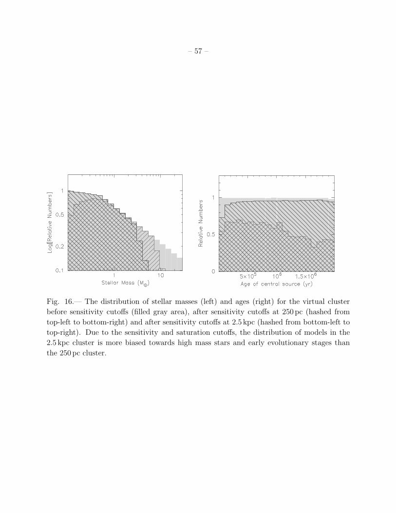
– 57 –

Fig. 16.— The distribution of stellar masses (left) and ages (right) for the virtual cluster

before sensitivity cutoffs (filled gray area), after sensitivity cutoffs at 250 pc (hashed from

top-left to bottom-right) and after sensitivity cutoffs at 2.5 kpc (hashed from bottom-left to

top-right). Due to the sensitivity and saturation cutoffs, the distribution of models in the

2.5 kpc cluster is more biased towards high mass stars and early evolutionary stages than

the 250 pc cluster.

– 58 –

Fig. 17.— JHK, IRAC, and IRAC+MIPS 24µm color-color plots for all the model SEDs

in the grid, showing the number of models on a logarithmic grayscale. The grayscale is

shown down to 0.01 % of the peak value. The reddening vector shows an extinction of

AV = 20, assuming the Indebetouw et al. (2005) extinction law. The dashed lines in the

JHK color-color plots show the locus of the reddened stellar photospheres. The solid lines

in the IRAC color-color plots show the “disk domain” and the domain of embedded young

objects (redward of the “disk domain”) from Allen et al. (2004) and Megeath et al. (2004).

– 59 –

Fig. 18.— Color plots for all the model SEDs showing from left to right: the ratio of the

number of Stage I models to all models, the ratio of the number of Stage II models to

all models, and the ratio of the number of Stage III models to all models. From top to

bottom: JHK color-color plots, IRAC color-color plots, and IRAC+MIPS 24µm color-color

plots. The reddening vector shows an extinction of AV = 20, assuming the Indebetouw

et al. (2005) extinction law. The red lines in the JHK color-color plots show the locus of the

reddened stellar photospheres. The blue lines outline the regions shown in Figure 23.

– 60 –

Fig. 19.— As for Figure 17 for the virtual cluster at 250 pc including sensitivity and satura-

tion cutoffs.

– 61 –

Fig. 20.— As for Figure 18 for the virtual cluster at 250 pc including sensitivity and satura-

tion cutoffs.

– 62 –

Fig. 21.— As for Figure 17 for the virtual cluster at 2.5 kpc including sensitivity and satu-

ration cutoffs.

– 63 –

Fig. 22.— As for Figure 18 for the virtual cluster at 2.5 kpc including sensitivity and satu-

ration cutoffs.

– 64 –

Fig. 23.— Approximate regions of JHK (left), IRAC (center) and IRAC+MIPS 24µm (right)

color-color space where the different evolutionary stages lie. From dark to light gray: the

regions where most models are Stage I, II, and III respectively. The hashed region in the

JHK and IRAC color-color plots are regions where models of all evolutionary stages can be

present. The dark gray region in the JHK color-color plot is also hashed to indicate that this

region, although never occupied by Stage II and III models in the absence of extinction, would

easily be contaminated by Stage II and III models for high values of extinction. The Stage II

area in the IRAC color-color plot is hashed to show that although most models in this region

are Stage II models, Stage I models can also be found with these colors. The orange region

in the JHK color-color plot represents the location of reddened stellar photospheres. The

yellow disk in the IRAC and IRAC+MIPS 24µm color-color plots represents the approximate

location of stellar photospheres in the absence of extinction. The blue rectangles show the

approximate regions where only disks with large inner holes lie. The reddening vectors show

an extinction of AV = 20, assuming the Indebetouw et al. (2005) extinction law.

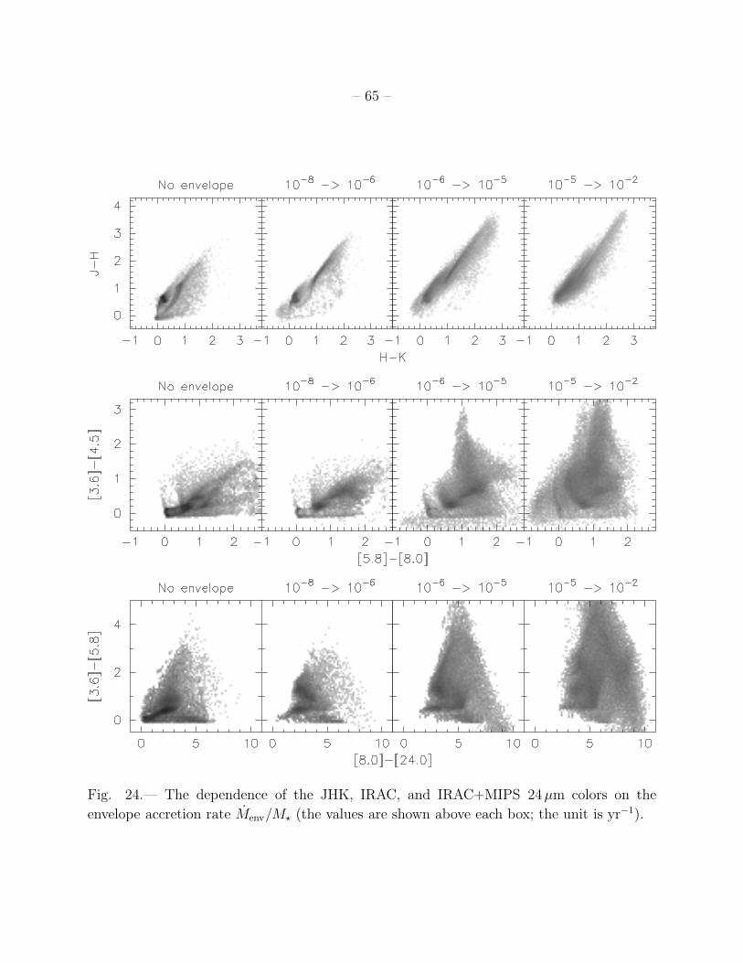
– 65 –

Fig. 24.— The dependence of the JHK, IRAC, and IRAC+MIPS 24µm colors on the

envelope accretion rate Menv/M� (the values are shown above each box; the unit is yr−1).

– 66 –

Fig. 25.— The dependence of the JHK, IRAC, and IRAC+MIPS 24µm colors on the disk

mass Mdisk/M� (the values are shown above each box). All Stage II models in the model

grid are shown.

– 67 –

Fig. 26.— The dependence of the JHK, IRAC, and IRAC+MIPS 24µm colors on the stellar

temperature T� (the values are shown above each box). All Stage I models in the model grid

are shown.

– 68 –

Fig. 27.— The dependence of the JHK, IRAC, and IRAC+MIPS 24µm colors on the stellar

temperature T� (the values are shown above each box). All Stage II models in the model

grid are shown.

– 69 –

Fig. 28.— The dependence of the JHK, IRAC, and IRAC+MIPS 24µm colors on the disk

and envelope inner radii Rmindisk (= Rmin

env ) (the values are shown above each box - the unit is

the dust sublimation radius Rsub). All the models from the grid are shown.