Interpreting sound signal formulae

Matias Dahl, Ville Turunen

19.3.2004

In our examples, a sound signal is represented as a function

g : R → [−1, 1],

where the real variable is time (measured in seconds), and the value g(t0) refers toa non-scaled deviance from the surrounding air pressure at time t0.

The standard air pressure is 1013 mBar (millibars). For human beings, the thresholdof pain at audible frequencies corresponds to the air pressure variation of less than1 mBar. Consequently, we may think that g(t) corresponds to the air pressure

(1013 + g(t)) mBar.

The threshold of hearing at audible frequencies is roughly 10−6 mBar (i.e. 0.000001mBar, a millionth of 1 mBar), so that a vibration g with the amplitude lower than10−6 is inaudible as far as we can tell.

The frequency of a sound signal within a time period is the momentary number ofoscillations per second, measured in Hertz, abbreviated Hz. This is readily under-stood for sinusoidal vibrations like

g(t) = sin(kt) :

here the frequency is k/(2π) Hz, where π ≈ 3.14159. For humans, audible fre-quencies range from 20 to 20000 Hz. Now let the signal g have the form

g(t) = sin(w(t))

for some smooth-enough function w : R → R. If w is increasing or decreasingwithin the time period [t0, t0 + h], then there are about |w(t0 + h) − w(t0)|/(2π)vibrations during this time interval of h seconds. Thus, within this time interval theaverage frequency is

|w(t0 + h) − w(t0)|2πh

,

1

and if we let the variable h tend to 0, we get the frequency of the signal g at the timeinstant t0:

limh→0

|w(t0 + h) − w(t0)|2πh

=|w′(t0)|

2π;

the instantaneous frequency is the absolute value of the derivative of w divided by2π.

Sound signals

The sampling rate is 1/δ = 44100 Hz and the unit for the variable t is seconds.

White noise (4a)

The characteristic for the white noise is that the samples of the signal are uncor-related random numbers distributed uniformly over [−1, 1]. Thus this noise doesnot vary in time, and all the possible frequencies are present with equal magnitude;the closest everyday instance is the sound of an untuned TV or radio channel. Thenoises encountered in nature are typically coloured, i.e. some frequency ranges areprevalent: for instance, a hum of a wind, sizzling of boiling water, etc.

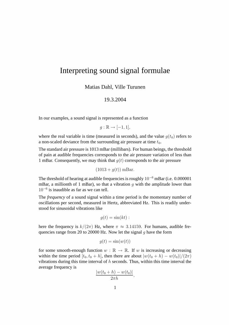
S1 (2c) and S

1000000 (1d)

Of the nine sounds, only two were instrumental-like. These are the sounds of S1

and S1000000 ringing. To distinguish these two from each other, a first observation

is that one signal sounded like a plucked string and the other like a bell. We knowthat plucked string instruments have harmonic overtones. It also holds that bells(together with gongs) do not have harmonic overtones. Suppose ∆ is the Laplaceoperator on S

n with respect of the metric induced from Rn+1. We assume known

that the eigenvalues of −∆ on S1 are 1, 2, 3, . . .. This implies that the sound of S

1

has harmonic overtones. From this it follows that S1 has the sound of a plucked

string. Therefore, by exclusion, S1000000 must sound like a bell.

Generally, the eigenvalues of −∆ on Sn are λk =

√

k(k + n − 1) for k = 0, 1, 2, . . .,and the sound of S

n was defined as

g(t) = e−t

∞∑

k=1

2−k sin(

2π220λk

λ1

t)

.

Here, we have normalized the eigenvalues, such that the fundamental frequency ofthe signal is always 220 Hz. For n = 1, we obtain λk

λ1

= 1, 2, 3, . . .. On the other

2

0 1 2 3 4 5 6 7−1

−0.8

−0.6

−0.4

−0.2

0

0.2

0.4

0.6

0.8

1

Time [s]

Am

plitu

de

0 1 2 3 4 5 6 7 8 9 10−1

−0.8

−0.6

−0.4

−0.2

0

0.2

0.4

0.6

0.8

1

Time [ms]

Am

plitu

de

Figure 1: Exponential decay of the S1 signal(2c) and the first 10 ms of the signal.

3

0 10 20 30 40 50 60 70 80 90 100−1

−0.8

−0.6

−0.4

−0.2

0

0.2

0.4

0.6

0.8

1

Time [ms]

Am

plitu

de

Figure 2: First 100 ms of the S1000000 vibrations (1d). In this signal, there is no

period.

hand, when n is very large, we have

λk

λ1

=

√

k(k + n − 1)

n

=

√

k2 − k

n+ k

≈√

k,

so S1000000 does not have harmonic overtones.

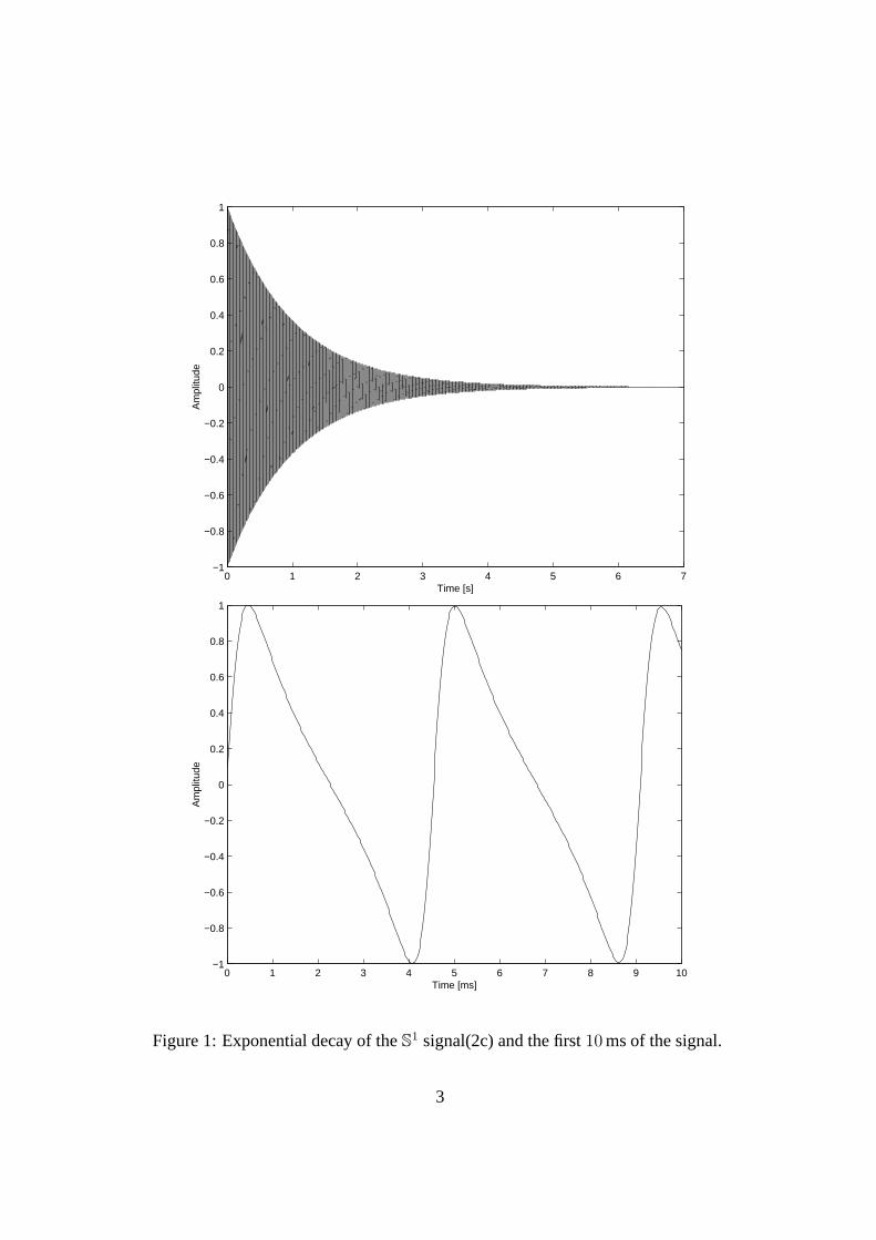
Amplitude modulation (6e)

g(t) =sin

(

40 sin(2π10t))

1 + sin sin t.

This signal was the only signal with a clear variation in volume. This can be seenfrom the relatively slowly oscillating denumerator, which varies between 1−sin 1 ≈0.16 and 1 + sin 1 ≈ 1.84. See Figure 3.

4

0 5 10 15 20 25 30−1

−0.8

−0.6

−0.4

−0.2

0

0.2

0.4

0.6

0.8

1

Time [s]

Am

plitu

de

0 0.05 0.1 0.15−1

−0.8

−0.6

−0.4

−0.2

0

0.2

0.4

0.6

0.8

1

Am

plitu

de

Time [s]

0 0.05 0.1 0.150

50

100

150

200

250

300

350

400

Inst

anta

neou

s fr

eque

ncy

[Hz]

Time [s]

Figure 3: The first figure shows the amplitude modulation (6e), the second showsthe signal for the first 100 ms, and the last shows the instantaneous frequency overthe first 0.15 s.

5

Topologist’s sinusoid (7b)

g(t) = sin(

2π 501

t

)

.

At t = 0, the signal has infinite instantaneous frequency, which smoothly dropsbelow the audible range in less than 2 seconds. This results into a familiar sci-fisound effect. See Figure 4.

Karplus–Strong (5i)

g(t) =

{

sin 9πt

2∆, when t < ∆,

1

2

(

g(t − ∆) + g(t + δ − ∆) · (S ◦ g)(t − ∆))

, when t ≥ ∆.

Here ∆ = 10 ms and S(t) = sign sin sinh(100 t).

This function is an implementation of the Karplus-Strong algorithm, which is astandard algorithm for producing plucked string and drum sounds. The algorithmstarts with an initial signal (here sin 9πt

2∆for t ∈ (0, ∆)), which is inductively mutated

using the lower branch in the definition. With good accuracy, S randomly takesvalues +1 and −1. Thus in the copy process, the signal is randomly passed througha lowpass filter (when S = 1), or a highpass filter (when S = −1). In effect, thesound becomes noisier over time while its amplitude decays. See Figure 5.

Recurring pulse with increasing frequency (3f)

g(t) = sin

(

2π100 sin50

(

2 sinht

4

) )

.

Since sin50 is almost zero for most of the time, this signal contains pulses, and sincesinh grows exponentially, these pulses become more frequent over time. Also, fromthe expression for the instantaneous frequency, one can see that the frequency of thesignal grows exponentially. This effect can be seen in Figure 6.

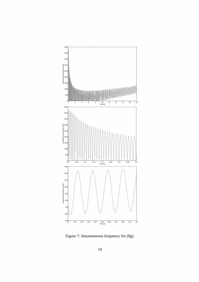
Frequency modulation (8g)

g(t) = sin(

150t2 + 70 sin(2π 40√

t))

.

For this sound, the instantaneous frequency is∣

∣

∣

∣

1

2π

(

300t + 2800πcos(2π40

√t)√

t

)∣

∣

∣

∣

.

6

0 1 2 3 4 5 6 7 8 9 10−1

−0.8

−0.6

−0.4

−0.2

0

0.2

0.4

0.6

0.8

1

Time [s]

Am

plitu

de

0.05 0.1 0.15 0.2 0.25 0.3 0.35 0.4 0.45 0.50

2000

4000

6000

8000

10000

12000

14000

16000

18000

Time [s]

Inst

anta

neou

s fr

eque

ncy

[Hz]

Figure 4: Topologist’s sinusoid (7b): entire signal and a plot of the instantaneousfrequency.

7

0 0.05 0.1 0.15−1

−0.8

−0.6

−0.4

−0.2

0

0.2

0.4

0.6

0.8

1

Time [s]

Am

plitu

de

0 0.005 0.01 0.015 0.02 0.025 0.03 0.035 0.04−1

−0.8

−0.6

−0.4

−0.2

0

0.2

0.4

0.6

0.8

1

Time [s]

Am

plitu

de

Figure 5: Karplus-Strong (drum sound) (5i).

8

0 2 4 6 8 10 12 14 160

1000

2000

3000

4000

5000

6000

Time [s]

Inst

anta

neou

s fr

eque

ncy

[Hz]

Figure 6: Instantaneous frequency for (3f).

Due to the 1√t-term, the signal starts with infinite frequency which rapidly drops.

For large t, the 300t-term dominates. The overall effect is that the instantaneousfrequency is oscillating and the longterm average frequency is slowly rising. Thiscan be seen in Figure 7.

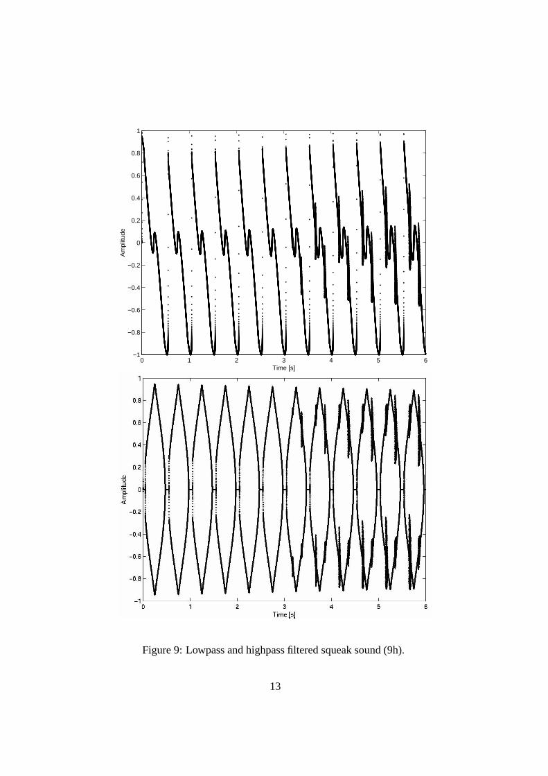
Squeak sound (9h)

g(t) =

{

0, when t < 0,sin

(

4πt + g(t − 3δ) − t

20g(t − 2δ) + g(t − δ)

)

, when t ≥ 0.

Using induction, one may show that g is continuous. Moreover, g is infinitelysmooth except for t = 0,±δ,±2δ, . . ..

Here, we have sampled the function at t = 0, δ, 2δ, . . ., that is, at the points whereg is continuous, but not necessarily smooth. This sound contains periodic clicksoccurring twice a second. It can therefore be recognized from the 4πt term.

To analyze this sound, let us define highpass and lowpass filters Hδ and Lδ, respec-

9

0 2 4 6 8 10 12 14 16 18 200

500

1000

1500

2000

2500

3000

3500

4000

4500

Time [s]

Inst

anta

neou

s fr

eque

ncy

[Hz]

0.1 0.15 0.2 0.25 0.3 0.35 0.4 0.45 0.50

500

1000

1500

2000

2500

3000

3500

4000

4500

Time [s]

Inst

anta

neou

s fr

eque

ncy

[Hz]

19 19.1 19.2 19.3 19.4 19.5 19.6 19.7 19.8 19.9 20500

600

700

800

900

1000

1100

1200

1300

Time [s]

Inst

anta

neou

s fr

eque

ncy

[Hz]

Figure 7: Instantaneous frequency for (8g).

10

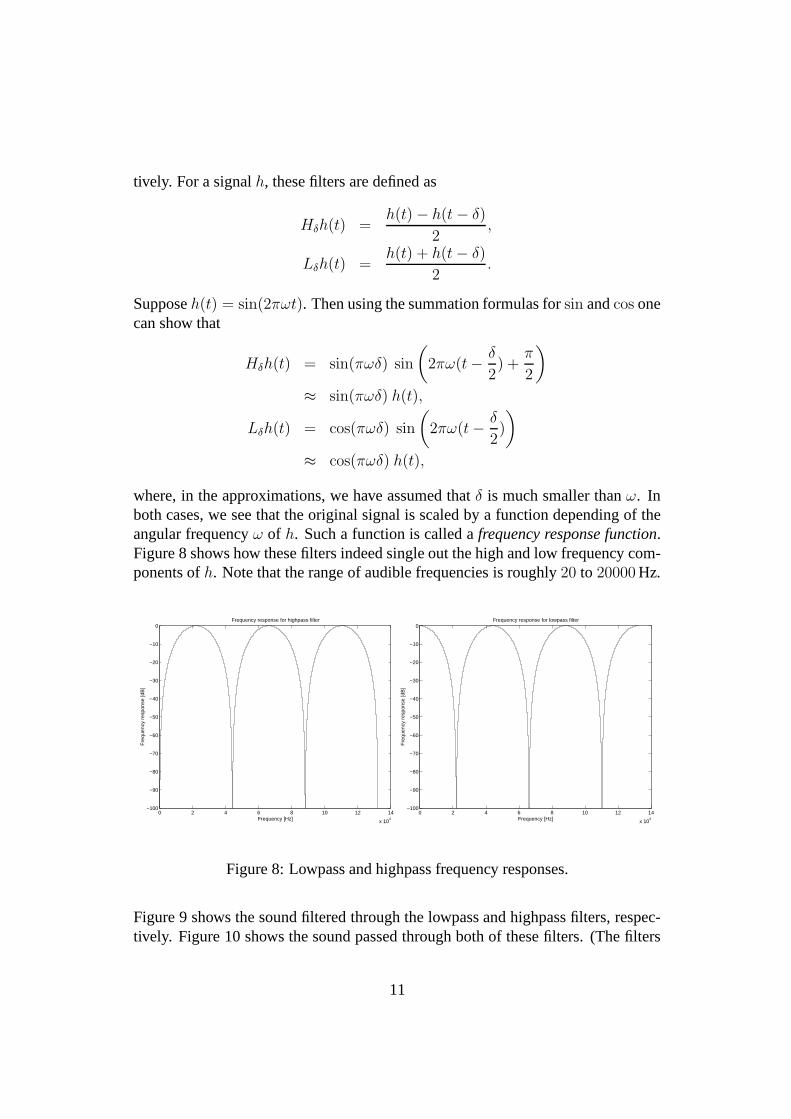
tively. For a signal h, these filters are defined as

Hδh(t) =h(t) − h(t − δ)

2,

Lδh(t) =h(t) + h(t − δ)

2.

Suppose h(t) = sin(2πωt). Then using the summation formulas for sin and cos onecan show that

Hδh(t) = sin(πωδ) sin

(

2πω(t − δ

2) +

π

2

)

≈ sin(πωδ) h(t),

Lδh(t) = cos(πωδ) sin

(

2πω(t − δ

2)

)

≈ cos(πωδ) h(t),

where, in the approximations, we have assumed that δ is much smaller than ω. Inboth cases, we see that the original signal is scaled by a function depending of theangular frequency ω of h. Such a function is called a frequency response function.Figure 8 shows how these filters indeed single out the high and low frequency com-ponents of h. Note that the range of audible frequencies is roughly 20 to 20000 Hz.

0 2 4 6 8 10 12 14

x 104

−100

−90

−80

−70

−60

−50

−40

−30

−20

−10

0

Frequency [Hz]

Fre

quen

cy r

espo

nse

[dB

]

Frequency response for highpass filter

0 2 4 6 8 10 12 14

x 104

−100

−90

−80

−70

−60

−50

−40

−30

−20

−10

0

Frequency [Hz]

Fre

quen

cy r

espo

nse

[dB

]

Frequency response for lowpass filter

Figure 8: Lowpass and highpass frequency responses.

Figure 9 shows the sound filtered through the lowpass and highpass filters, respec-tively. Figure 10 shows the sound passed through both of these filters. (The filters

11

commute, LδHδ = HδLδ = 1

2H2δ, so the order is irrelevant.) In Figure 10, the

clicks and squeaks are clearly seen.

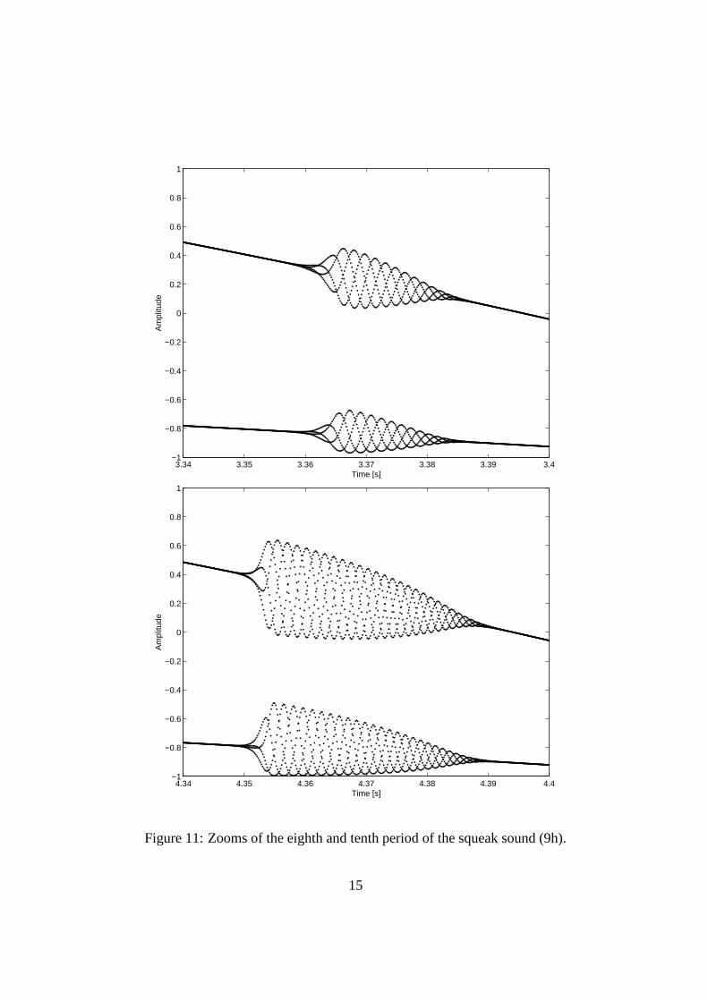
Figure 11 shows zooms of some squeaks in the original signal.

12

0 1 2 3 4 5 6−1

−0.8

−0.6

−0.4

−0.2

0

0.2

0.4

0.6

0.8

1

Time [s]

Am

plitu

de

Figure 9: Lowpass and highpass filtered squeak sound (9h).

13

0 1 2 3 4 5 6−0.3

−0.2

−0.1

0

0.1

0.2

0.3

0.4

Time [s]

Am

plitu

de

Figure 10: Squeak sound (9h), both lowpass and highpass filtered.

14

3.34 3.35 3.36 3.37 3.38 3.39 3.4−1

−0.8

−0.6

−0.4

−0.2

0

0.2

0.4

0.6

0.8

1

Time [s]

Am

plitu

de

4.34 4.35 4.36 4.37 4.38 4.39 4.4−1

−0.8

−0.6

−0.4

−0.2

0

0.2

0.4

0.6

0.8

1

Time [s]

Am

plitu

de

Figure 11: Zooms of the eighth and tenth period of the squeak sound (9h).

15