interpretable classiﬁcation of bacterial raman spectra

1

Interpretable Classification of Bacterial RamanSpectra with Knockoff Wavelets

Charmaine Chia∗, Matteo Sesia∗, Chi-Sing Ho, Stefanie S. Jeffrey, Jennifer Dionne,Emmanuel J. Candes, and Roger T. Howe

Abstract—Deep neural networks and other sophisticated ma-chine learning models are widely applied to biomedical signaldata because they can detect complex patterns and computeaccurate predictions. However, the difficulty of interpreting suchmodels is a limitation, especially for applications involving high-stakes decision, including the identification of bacterial infections.In this paper, we consider fast Raman spectroscopy data anddemonstrate that a logistic regression model with carefullyselected features achieves accuracy comparable to that of neuralnetworks, while being much simpler and more transparent.Our analysis leverages wavelet features with intuitive chemi-cal interpretations, and performs controlled variable selectionwith knockoffs to ensure the predictors are relevant and non-redundant. Although we focus on a particular data set, theproposed approach is broadly applicable to other types of signaldata for which interpretability may be important.

Index Terms—Machine learning, Interpretability, Knockoffs,False discovery rate, Raman spectroscopy.

I. INTRODUCTION

NEW sensor technologies have contributed to the adventof “big data” in biomedicine, of which signal data are

an important modality. From one-dimensional electrocardiog-raphy and electroencephalography signals from the heart andbrain, to two-dimensional tissue images of tumor histology, tothree-dimensional magnetic resonance images, these consistof sequential measures of an observable along one or moreindependent axes such as time, distance, or frequency. Signaldata differ from structured forms of data in that the meaning ofeach independent variable is not as distinctively and intuitivelydefinable. Informative features must be extracted using signalprocessing and machine learning (ML) techniques before use-ful patterns can be detected and leveraged to make predictions.

∗Equal contribution.This work was partly supported by NSF grants DMS 1712800 and

1934578, a Math+X grant (Simons Foundation), and by the Stanford Schoolof Engineering’s Catalyst for Collaborative Solutions. The authors thankthe Research Computing Center at Stanford University and the Center forAdvanced Research Computing at the University of Southern California forproviding computing resources.

C. Chia (email: [email protected]) was in the Department ofElectrical Engineering at Stanford University, Stanford, CA 94305, coadvisedby R. T. Howe and S. S. Jeffrey. She is now with Aether Biomachines, MenloPark, CA 94025 USA.

M. Sesia (email: [email protected]) was in the Department of Statis-tics at Stanford University, advised by E. Candes. He is now in the Departmentof Data Sciences and Operations at the University of Southern California, LosAngeles, CA 90089 USA.

C-S. Ho was in the Department of Applied Physics at Stanford University,advised by J. Dionne. She is now with Tempus Labs, Redwood City, CA94065, USA.

While predictive accuracy is usually prioritized in ML,model interpretability is gaining more attention. Interpretabil-ity is crucial when models inform the decisions of expertsand can have serious consequences, such as in applicationsinvolving healthcare. Furthermore, when the signal sourceitself is not well-understood, interpretable models can yielddeeper insights and facilitate inferences. Along these lines,the ML framework discussed in [1] proposes three metrics forevaluating models: 1) predictive accuracy (the goodness-of-fitto the underlying data), 2) descriptive accuracy (the fidelity ofthe interpretation in describing relations learned by the model),and 3) relevancy (the usefulness and comprehensibility of theinterpretation to the target audience).

Simpler models (e.g., linear regression, trees, naive Bayes)are easier to interpret, though often at the expense of pre-dictive accuracy due to their limited flexibility. By contrast,sophisticated models such as deep neural networks [2–4] canautomatically extract predictive features and capture complexrelations in the data, but their “black-box” nature makes itdifficult to understand their decisions. Various techniques havebeen proposed to improve the descriptive accuracy of MLmodels; for example, saliency methods help visualize theactivation of individual input features [5], while attributionmethods like LIME [6] and SHAP [7] quantify the impact ofeach feature on the output predictions. However, these post hoctechniques are not designed for developing simpler models.

With regard to relevancy, studies report that people favorexplanations that are short, contrast instances with differentoutcomes, and highlight abnormal causes [8]. In other words,we seek to understand which features are important, andhow these affect the outcome. Data scientists often pursuethese goals through feature selection, in addition to featureextraction, to ensure that their conclusions are based onrelevant and non-redundant predictors. For example, one maywant to identify a smaller set of genetic variants linked todisease susceptibility among thousands of possibilities [9], orto identify which specific morphological features from brainelectroencephalogram signals can diagnose epilepsy [10].

There exists a broad literature on variable selection methodsdesigned to identify a subset of important and non-redundantpredictors from a large set of features; see [11–14] for anoverview. However, most existing techniques are either heuris-tic, in the sense that they lack clear statistical guarantees,or require asymptotic approximations and strong modelingassumptions, which may not be justified when working withcomplex biomedical data. Consequently, tuning these modelsthrough variable selection may be difficult and their output

arX

iv:2

006.

0493

7v3

[ee

ss.S

P] 2

May

202

1

2

may include unexpected numbers of false discoveries: unim-portant features that are either irrelevant or redundant (seeAppendix A for a more precise definition of this concept).For example, the lasso is a very successful variable selectionmethod for high-dimensional linear models [15] and it isknown to be asymptotically consistent under certain assump-tions [16, 17]; it tends to select all relevant non-redundantfeatures as the sample size grows. In practice, however, it oftenutilizes more predictors than necessary. Feature selection be-comes even more challenging when it involves non-parametricmodels, although some theoretical results have been obtainedfor random forests [18], and several proposals have beenadvanced for sparse neural networks [19–21].

A general approach to variable selection with a clear statis-tical interpretation is offered by the knockoff filter; this wasfirst proposed in the context of linear regression [22] and laterextended to general machine learning algorithms [23], includ-ing the classification ones considered in this paper. The mainidea of this solution is to augment the available features withan equal number of synthetic negative controls (the knockoffs).Knockoffs are constructed to be statistically indistinguishablefrom those variables among the original ones that are unimpor-tant [23]; however, the identities of the knockoffs are knownexactly, unlike those of the latter. Therefore, the importantfeatures can be selected by looking for those that significantlystand out from the knockoffs [22]. See Appendix A for areview of this method. Under relatively mild assumptions, theknockoff filter is guaranteed to control the false discovery rate(FDR) [24]: the expected proportion of irrelevant or redundantfeatures among the selected ones. Knockoffs can be appliedwith any machine learning algorithm and require no modellingassumptions about the unknown relation between the availablefeatures and the true bacterial classes. This flexibility makesknockoffs particularly well-suited to our problem becausebacterial classification is an inherently complex task withimplications for patient treatment, making robustness andinterpretability important considerations. Furthermore, control-ling the FDR is a reasonable objective in our context becausewe seek to construct predictive models that are both accurate,leveraging all relevant information, and simple to explain,avoiding unnecessary features.

Previous applications of knockoffs have focused on struc-tured data, in which the features are well-defined a priori:single-nucleotide polymorphisms [9, 25–28], virus mutations[29], or demographic/behavioral cancer biomarkers [30], toname some examples. Only few extensions to unstructureddata have been reported, namely involving computed tomog-raphy (CT) [31], functional magnetic resonance images [32],and economic time series [33]. Thus, the relatively unexploredarea of unstructured data provides an interesting use case.

In this paper, we combine feature extraction and selectionto obtain a powerful and interpretable signal analysis method,and demonstrate its utility by applying it to a data set offast Raman spectroscopy measurements of common bacteriacollected at the Stanford Hospital [34]. Raman spectroscopymeasures the interaction of laser light with a sample, produc-ing a spectrum where peaks indicate wavelengths at whichthe light is strongly absorbed by the chemical bonds present

therein. This technique thus yields an optical fingerprint of thesample. Fast Raman measurements follow the same principle,but their spectra are noisier and more difficult to recognizedue to shorter measurement times. Therefore, reliable MLalgorithms are useful to automate the recognition of suchoptical fingerprints. Recently, a convolutional neural network(CNN) was found to be successful at using these data to predictoutcomes such as bacterial strain and antibiotic susceptibility[34]. These results are promising because rapid and culture-free pathogen identification could advance the treatment ofbacterial infections and sepsis. At the same time, such high-stakes medical decisions call for more interpretable modelsthat can be easily examined and understood by humans who,for instance, may wish to know the presence of which chemicalbonds drives the machine decision.

Our approach begins with a feature extraction step thattransforms the signal data into a more intuitive representationsummarizing the presence of localized peaks in the spectra.Then, we apply the knockoff filter to select a subset of featuresthat are likely to be predictive and non-redundant, and finallywe use these to fit a simple multinomial logistic regressionmodel that predicts the outcome of interest. Our analysis showsthat the proposed method performs similarly to the CNN of[34] in terms of predictive accuracy, and sometimes evenbetter, while creating a more compact and interpretable model.

II. DATA SETWe analyze data consisting of 60,000 Raman spectra of

dried monolayer bacteria and yeast samples taken with fast(one-second) scans, from [34]. Thirty distinct isolates weremeasured, including multiple isolates of Gram-negative andGram-positive bacteria, as well as Candida species; 2000spectra were measured for each isolate, most of which weretaken over single cells. The spectra consist of 992 mea-surement points evenly distributed in the spectral range of381.98 to 1792.4 cm−1. The measured Raman intensities werenormalized to lie between 0 and 1. Further details aboutthese measurements can be found in [34]. The data can bedownloaded from https://github.com/csho33/bacteria-ID.

In addition to the Raman spectra (X), three sets of associ-ated outcome labels (Y ) are available from this data set:

1) Isolate labels → 30 classes;2) Empiric antibiotic treatment → 8 classes;3) Methicillin resistance of Staphylococcus aureus strains→ 2 classes

To summarize, the sizes of the data matrices are:• Raw signal data (X): 60, 000× 992;• Outcome labels (Y ): 60, 000×1, except for the 3rd set of

labels, which apply only to Staphylococcus aureus strains,giving a 10, 000× 1 outcome matrix.

The code to reproduce our analysis is available from https://github.com/chicanagram/raman-knockoffs.

III. METHODSA. Feature extraction

Feature extraction is the transformation of raw data intoa more discriminatory representation for the prediction task.

https://github.com/csho33/bacteria-ID

https://github.com/chicanagram/raman-knockoffs

https://github.com/chicanagram/raman-knockoffs

3

There exist a variety of feature extraction methods for signaldata, which can be categorized into four broad families [2].

1) Time/position methods extract characteristic propertiesfrom specific windows of measurement points.

2) Frequency methods break signals into their spectralcomponents, giving information complementary to theabove; e.g., the Fourier transform [35].

3) Time/position-frequency methods capture both fre-quency and time/position information in non-linear andnon-stationary signals; e.g., the wavelet transform [36].

4) Sparse signal decomposition methods seek sparse datarepresentations in terms of basis sets that are definedempirically; e.g., convolutional dictionary learning [37].

In general, different feature extraction methods may be bet-ter suited for different kinds of data, and they should be chosenbased on their natural interpretability given the dynamics ofthe signal source or other relevant prior knowledge [2]. In ourapplication, we opt for a discrete wavelet transform (DWT),which projects the signal X onto a compact orthogonal basisset of wave-like oscillations at different frequencies, beginningand ending with zero amplitude. The ability of wavelets tocapture both frequency and location information is critical tothe analysis of Raman spectral data. In fact, the features ofnatural interest there are the localized peaks indicating thepresence of chemical bonds which may distinguish differenttypes of bacteria. Moreover, the DWT provides a compactrepresentation of the signal which can be computed efficiently,unlike the continuous wavelet transform. The basis waveletwe adopt is a 24-point Coiflet with five DWT levels [38].This choice is motivated by the symmetry of coiflets, whichfacilitates their comparison with the resonance peaks in thespectra clearly visible to the naked eye [39]. The filter length(24 points) and number of decomposition levels were chosen tomatch as well as possible the visible peaks in our spectra. Thistuning was carried out manually, visualizing the basis waveletsalongside de-noised signals obtained by averaging fast Ramanspectra from multiple bacterial samples from within the sameclass. The result of the transform, X ′, is a set of 1105features for each of the 60,000 samples, which represent theconcatenated approximation and detail coefficients from thefive-level wavelet filtering procedure. Starting from the waveletrepresentation, the original signal can be reconstructed usingan Inverse Discrete Wavelet Transform (IDWT).

B. Knockoff generation

We generate knockoffs for both the raw data (X) and thewavelet features (X ′) following the model-X method in [23],as implemented by the second-order knockoff machines in[29]; see Appendix A for relevant technical background. Weapply this algorithm to generate knockoffs that are approxi-mately pairwise exchangeable with the data in terms of theirsecond moments. More precisely, we generate the knockofffeatures X ∈ Rn×p given the original features X ∈ Rn×p (or,analogously, X ′) such that the mean vector and the covariancematrix of [X, X] ∈ Rn×2p match those of [X, X]swap(j), forany j ∈ {1, . . . , p}. Above, swap(j) is the operator that swapsXj with Xj . Simultaneously, we try to make each element of

X as different as possible from the corresponding element ofX [23, 29], to maximize the statistical power of the knockofffilter [22]. By such construction, the covariance matrices of[X, X] and [X, X]swap(j), for any j, are approximately

G =

[Σ Σ− diag(s)

Σ− diag(s) Σ

], (1)

where Σ is the covariance matrix of X and the vector s ismaximized subject to the constraint that the matrix G bepositive semi-definite [22, 23]. We refer to [23] and [29]for further details on knockoff generation. It is worth men-tioning the method in [29] can accommodate a more generalconstruction that also matches higher moments of [X, X] tothose of [X, X]swap(j), which leads to a more robust variableselection procedure in some situations, but seems to make littledifference with our data. Therefore, we focus on second-orderknockoffs for simplicity.

C. Feature selection with the knockoff filter

Following the generation of knockoffs, 80% of the datapoints are randomly assigned to a training set, and the re-maining 20% are assigned to a test set, which will be utilizedonly later to evaluate predictive performance, similarly to [40].The augmented raw and wavelet representation training data,[X, X] and [X ′, X ′], are standardized to make their columnshave unit variance, and then they are separately provided asinput to a classifier, which is trained on each of the threesets of the corresponding Y labels. The number of featuresavailable to each model is thus twice that of the original data.The classification model is based on logistic regression with`1 (lasso) regularization [15], which results in sparse modelswith several coefficients equal to zero, thus already performingfeature selection to some degree. For the 30-class isolateidentification and 8-class antibiotic treatment classificationtasks, we use a multinomial logistic regression model [41],which outputs a probability distribution across all the classes;the class with the largest estimated probability is taken asthe final prediction. For the 2-class methicillin resistanceclassification, standard (binomial) logistic regression is used.

The logistic regression models are fitted using the glmnetR package [42]. We denote the estimated coefficients foreach task as β1(λ), . . . , β2p(λ); the parameter λ controls thestrength of the `1 penalty and is tuned by 10-fold cross-validation. Note that, for the multinomial models, we use an“ungrouped” `1 penalty, so that all individual regression taskswithin the multinomial model are penalized independently.This leads to the selection of more features overall, althoughit turns out to yield significantly more accurate predictionsfor these data compared to the alternative “grouped” penalty.See [42] for more details on how these models are estimated.The βj(λ) and βj+p(λ) coefficients are used to define a score,namely Wj = |βj(λ)| − |βj+p(λ)|, for each of the p originalfeatures, as explained further in Appendix A. Feature selectionis then performed by selecting variables with Wj ≥ T , whereT is a data-adaptive threshold computed by the knockofffilter [22] to control the FDR below 10%, so that we canexpect about 90% of the selected features to be important or

4

redundant [23]. We denote by S ⊆ {1, . . . , p}, or S′, the subsetof features thus selected from X , or X ′, respectively.

D. Classification

We compare the predictive performance of the featuresselected by the knockoff filter, {Xj}j∈S , {X ′j}j∈S′ , to thatof the full sets of raw and wavelet features, X,X ′. For thispurpose, we fit classification models based on `1-regularized(multinomial) logistic regression on the training data, as be-fore, for all 12 prediction tasks arising from combination ofthese four input data sets and the three sets of output labels:

X{Xj}j∈SX ′

{X ′j}j∈S′

×Y30−classY8−classY2−class

. (2)

Figure 1 summarizes the main steps of our analysis. The out-of-sample predictive performance is evaluated on the 20% ofobservations assigned to the test set. The entire analysis isrepeated five times, starting from the feature selection step,so that each sample in the full data set is assigned to the testset exactly once. This approach reduces the variability of ourfindings and facilitates the comparison with the benchmarksfrom [40]. Looking at the results from these 12 predictiontasks, we can evaluate both (A) the effect of applying featureextraction, and (B) the effect of feature selection via theknockoff filter. Finally, we compare the performance of ourmodels to previous results in [40], which were obtained using aCNN, a support vector machine (SVM), and logistic regressionmodels based on different features.

Fig. 1. Analysis framework for the interpretable classification of bacterialRaman spectra. First, wavelet features are extracted from the raw data; then,knockoffs are used to select a predictive and non-redundant subset of them;finally, a logistic regression model is fitted on the selected features.

IV. RESULTS AND DISCUSSION

Table I summarizes the prediction errors obtained by ourmethod for the three prediction tasks (30, 8, and 2 classes),using each of the four input data sets: X , {Xj}j∈S , X ′,{X ′j}j∈S′ . The prediction errors are defined as the misclassifi-cation rates, i.e., the proportions of data points with incorrectlypredicted labels. These results are averaged over the fivedisjoint test sets that we consider. The rows correspondingto results involving the knockoff filter are shaded and ar-ranged below those corresponding to results obtained without

TABLE IPERFORMANCES OF LOGISTIC REGRESSION MODELS BASED ON RAW AND

WAVELET FEATURES, BEFORE AND AFTER FEATURE SELECTION. THESERESULTS ARE AVERAGED OVER FIVE RANDOM TEST SETS (WITH

STANDARD DEVIATIONS IN PARENTHESIS).

Input Input features Nonzero coefficients Test error (%)

30 classesX 992 (0) 992 (0) 7.4 (0.2)

{Xj}j∈S 980 (2) 980 (2) 7.4 (0.2)X′ 1105 (0) 1018 (8) 6.8 (0.2)

{X′j}j∈S′ 136 (3) 136 (3) 5.1 (0.2)

8 classesX 992 (0) 991 (1) 5.6 (0.1)

{Xj}j∈S 949 (4) 949 (4) 5.5 (0.2)X′ 1105 (0) 1008 (4) 5.3 (0.2)

{X′j}j∈S′ 111 (8) 111 (8) 4.7 (0.3)

2 classesX 992 (0) 668 (36) 7.3 (0.6)

{Xj}j∈S 478 (38) 477 (37) 7.5 (0.6)X′ 1105 (0) 254 (107) 6.1 (0.4)

{X′j}j∈S′ 66 (8) 66 (8) 6.2 (0.3)

controlled variable selection. The third column counts thenumber of non-zero coefficients in the final regularized logisticregression model, which is fitted on the input features aftertuning the parameter λ by 10-fold cross-validation.

A. Effect of feature extraction

To examine the effect of feature extraction, we compare theclassification errors in Table I corresponding to the input datasets X and X ′ (in the white rows), for each of the three tasks.In each case, we observe a decrease in test error, from 7.4% to6.8% for the 30-class task, from 5.6% to 5.3% for the 8-classtask, and from 7.3% to 6.1% for the 2-class task.

As an additional comparison, Table II reports the predictiveperformance (within a regularized logistic regression model)of our wavelet features next to that of features obtained by per-forming a component analysis (PCA) on the raw signal data.(Recall that PCA extracts directions with maximal variance inthe data matrix.) To facilitate the comparison, the number ofprincipal components is fixed to match the number of waveletfeatures selected by the knockoff filter for each classificationtask. Again, the wavelet features yield lower classificationerrors, which should not be very surprising given that theyhave a much more intuitive interpretation for our kind of data.

B. Effect of feature selection

To examine the effect of feature selection with the knockofffilter, we compare the classification errors in adjacent pairsof rows in Table I, for each of the three tasks. In general,we observe that controlled feature selection with the knockofffilter can simultaneously improve interpretability, since modelsbased on fewer features are easier to explain, as well aspredictive accuracy. In particular, we see some improvementsin classification accuracy between X ′ and {X ′j}j∈S′ , as theknockoff filter selects a subset of the wavelet features beforethe final classifier is trained. The misclassification rate de-creases from 6.8% to 5.1% for the 30-class task, from 5.3% to

5

TABLE IIPERFORMANCES OF LOGISTIC REGRESSION MODELS BASED ON RAW-PCAAND KNOCKOFF-FILTERED WAVELET FEATURES. OTHER DETAILS ARE AS

IN TABLE I.

Input Input features Nonzero coefficients Test error (%)

30 classesXPCA136 136 (3) 132 (3) 5.4 (0.2){X′j}j∈S′ 136 (3) 136 (3) 5.1 (0.2)



4.7% for the 8-class task, and remains approximately constant(it increases slightly from 6.1% to 6.2%) for the 2-class task.These results are notable given that the numbers of features in-put into the classifier are reduced significantly: of the original1105 wavelet features, we are left with only 136, 111, and 66features for the respective tasks, on average. By contrast, thelasso model estimated without knockoff filtering assigns non-zero coefficients to as many as 1018 features (for the 30-classproblem), which will clearly make the interpretations morechallenging. We have also observed that a grouped `1 penalty,instead of the ungrouped one we adopted here, would resultin a lasso model with fewer variables, but at the cost of loweraccuracy. The benefits of controlled feature selection are lessobvious when this is applied to the raw signal data, X . In thiscase, the knockoff filter does not reduce the number of featuressignificantly, and the resulting changes in classification errorsare minimal. This suggests the wavelet features are muchmore informative, as fewer of them can achieve equivalent orpossibly higher accuracy compared to the raw signal variables.

C. Comparisons with other classifiers

Table III compares the performance of our method to thatof other classifiers applied to the same data. These bench-marks are a convolutional neural network (CNN), a supportvector machine (SVM), and logistic regression (LR) withoutregularization [40]. The CNN is applied directly to the rawsignals, while the SVM and LR take the top 20 principalcomponents as input features [40]. We denote our method asKWLR (knockoff-filtered wavelet logistic regression). Again,we report the average performance over five disjoint test sets,each containing 20% of the data points.

Our proposed method (KWLR) uses far fewer featurescompared to the benchmarks; such parsimony, combined withthe intuitive nature of the logistic regression model, makes ourapproach much more easily interpretable. Furthermore, KWLRleads to more accurate predictions for the 30-class task, whichis the most difficult one, yielding a misclassification ratethat is almost half that of the SVM and LR. The KWLRpredictions for the 8-class and 2-class prediction tasks are lessaccurate than those obtained with the CNN. This result maybe explained by noting that the signal-to-noise ratio is highercompared to the 30-class classification problem, as there are

TABLE IIICOMPARISON OF AVERAGE TEST ERRORS OBTAINED WITH OUR METHOD

TO THOSE CORRESPONDING TO OTHER MODELS. THE RESULTS IN THEWHITE ROWS ARE QUOTED FROM [40].

Input Classifier# ofinput

features

# ofnonzero

coefficients

Testerror(%)

Errors. d.(%)

30 classesX CNN 992 992 6.2 0.1

XPCA20 SVM 20 20 11.3 0.2XPCA20 LR 20 20 10.7 0.2{X′}j∈S′ KWLR 136 136 5.1 0.2

8 classesX CNN 992 992 1.0 0.1

{X′}j∈S KWLR 111 111 4.7 0.3

2 classesX CNN 992 992 4.6 0.5

{X′}j∈S′ KWLR 66 66 6.2 0.3

now more examples per class and clearer distinctions betweenthem. In this low-noise setting, the higher flexibility of theCNN provides the latter with an advantage, without necessarilyalso involving higher risk of overfitting. In any case, ourmethod achieves the primary goal set by this paper: weimprove interpretability, as our model is simpler and utilizesfar fewer features compared to the CNN, while achievingsatisfactory predictive accuracy.

Table IV in Appendix B compares the performances ofNaive Bayes and Nearest-Neighbor classification models basedon our wavelet features, before and after feature selection withknockoffs. These alternatives are simple and easy to interpret,but not as accurate as logistic regression. Nonetheless, featureselection with knockoffs still tends to relatively improve thepredictive accuracy of the Naive Bayes and Nearest-Neighbormodels, while also greatly reducing the number of featuresupon which their output depends. In conclusion, our resultssuggest logistic regression with the wavelet features selectedby the knockoff filter achieves the best trade-off betweeninterpretability and predictive accuracy for this data set.

D. Visualization of the wavelet features

Figure 2(a) shows an example of a raw Raman signal, whichwe denote as X(1). From this, we extract wavelet featuresX ′(1) and generate corresponding knockoffs X ′(1). Figure 2(b)shows the IDWT projection of X ′(1) back into the signaldomain. We observe that the knockoff signal preserves somecharacteristics of the original signal, such as its general shapeand noise pattern, but it is clearly distinct.

Figure 3 plots the correlations between the original fea-tures (a) and the cross-correlations between the original andknockoff wavelet features (b). The first 100 features or so,corresponding to the lower level DWT coefficients, show thestrongest local (among adjacent features) cross-correlations(see insets), while most other features are approximatelyuncorrelated. The property in (1), which follows from theconstruction of the knockoffs, implies that Figure 3(b) shouldlook very similar to Figure 3(a), except for the values on the

6

Fig. 2. (a) Raman signal, and (b) knockoff copy of its wavelet representation,projected back into the signal domain.

Fig. 3. Correlation map for (a) original wavelet features; (b) original andknockoff wavelet features. The inset highlights the first 100 features.

diagonal, which can be lower in (b). This suppression of thediagonal values reflects our attempt to make the knockoffs asdifferent as possible from the real features [23] (this can onlybe partly achieved for the first 100 wavelets because they havestronger correlations among themselves).

This second-order construction of knockoffs assumes a mul-tivariate Gaussian approximation for the feature distribution,which may not necessarily be very accurate. In any case, ourclassification results indicate that the second-order knockoffsare effective in performing controlled feature selection, whileretaining power in the selected features. The alternative knock-off construction described in [29] can model the underlyingfeature distribution more flexibly, which can make the FDRcontrol more robust if the features are non-Gaussian but didnot make a significant difference in this case.

Figure 4 visualizes a set of knockoff-filtered features in the

wavelet and signal domains, with the latter obtained throughan IDWT. Most of these wavelets are at lower frequency, asthe higher frequency one tend to be filtered out. Thus, mostnoise in the signal domain is removed, while certain peaks areaccentuated. Such peaks reveal interpretable structures that areimportant for bacterial classification, in a way that the noisyraw signal cannot directly capture. In particular, we expectpeaks in our Raman spectra to indicate distinguishing chemicalbonds found in different classes of bacteria.

Fig. 4. Visualization in the wavelet and signal domain of features selectedby the knockoff filter.

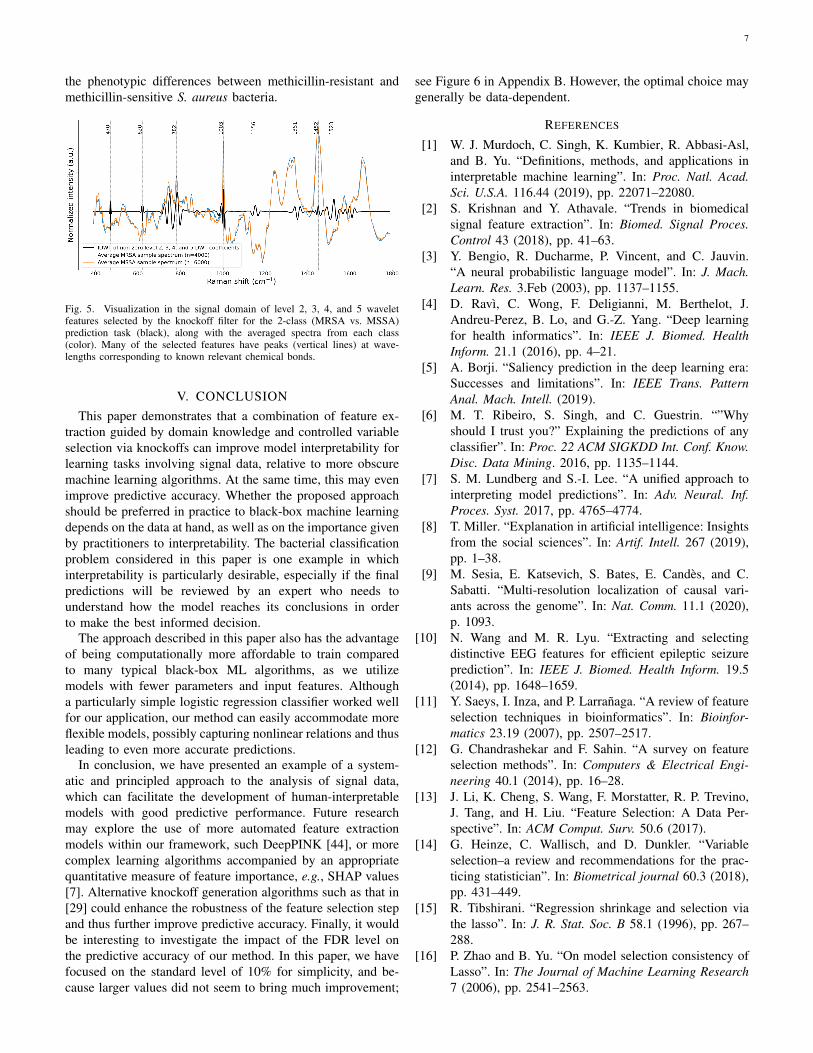
Examining the higher order (i.e., more spatially localized)wavelet features selected by our method for the 2-class task,we indeed observe these are consistent with peaks previ-ously identified as being relevant to discriminating betweenmethicillin-resistant (MRSA) and methicillin-sensitive strains(MSSA) of the Staphylococcus aureus bacteria [43]. Recallthat we say a feature is “selected” if its fitted coefficient isnon-zero after performing knockoff filtering and sparse logisticregression modeling. The non-zero detail coefficients fromlevels 2, 3, 4, and 5 of the wavelet transform for a singleMRSA sample are represented in Figure 4 by spikes in theblue, green, yellow, and red plots, respectively. Figure 5 showsthe IDWT of these features alongside the averaged spectrafrom each class. Specifically, it appears that level 2 waveletswith peaks close to 781 cm−1, 1004 cm−1, 1159 cm−1, and1523 cm−1 were selected. These correspond to the breathingmodes for the pyrimidine ring and phenylalanine, as well asthe C-C and C=C stretching modes for staphyloxanthin, acarotenoid pigment produced by S. aureus that gives it itscharacteristic golden color. Further, level 3 and 4 wavelets withpeaks around 1456 cm−1 and 1004 cm−1 were also selected,pointing to the CH2/CH3 bending mode and phenylalaninebreathing mode. These findings agree with the considerablyless noisy Raman microspectroscopy data in [43], which foundthat the ratios of the 1159 cm−1, 1523 cm−1, and 1456cm−1 peaks to the 1004 cm−1 peak were highly predictiveof methicillin resistance, and potentially also indicate differ-ences in pigmentation and lipid concentration in S. aureusstrains. In addition to these known peaks, we also observedthat level 5, 4, and 2 wavelets corresponding respectively topeaks around 470 cm−1, 620 cm−1, and 1351 cm−1 wereimportant. It is possible that future research will shed light ontheir chemical origins and allow us to more fully understand

7

the phenotypic differences between methicillin-resistant andmethicillin-sensitive S. aureus bacteria.

Fig. 5. Visualization in the signal domain of level 2, 3, 4, and 5 waveletfeatures selected by the knockoff filter for the 2-class (MRSA vs. MSSA)prediction task (black), along with the averaged spectra from each class(color). Many of the selected features have peaks (vertical lines) at wave-lengths corresponding to known relevant chemical bonds.

V. CONCLUSIONThis paper demonstrates that a combination of feature ex-

traction guided by domain knowledge and controlled variableselection via knockoffs can improve model interpretability forlearning tasks involving signal data, relative to more obscuremachine learning algorithms. At the same time, this may evenimprove predictive accuracy. Whether the proposed approachshould be preferred in practice to black-box machine learningdepends on the data at hand, as well as on the importance givenby practitioners to interpretability. The bacterial classificationproblem considered in this paper is one example in whichinterpretability is particularly desirable, especially if the finalpredictions will be reviewed by an expert who needs tounderstand how the model reaches its conclusions in orderto make the best informed decision.

The approach described in this paper also has the advantageof being computationally more affordable to train comparedto many typical black-box ML algorithms, as we utilizemodels with fewer parameters and input features. Althougha particularly simple logistic regression classifier worked wellfor our application, our method can easily accommodate moreflexible models, possibly capturing nonlinear relations and thusleading to even more accurate predictions.

In conclusion, we have presented an example of a system-atic and principled approach to the analysis of signal data,which can facilitate the development of human-interpretablemodels with good predictive performance. Future researchmay explore the use of more automated feature extractionmodels within our framework, such DeepPINK [44], or morecomplex learning algorithms accompanied by an appropriatequantitative measure of feature importance, e.g., SHAP values[7]. Alternative knockoff generation algorithms such as that in[29] could enhance the robustness of the feature selection stepand thus further improve predictive accuracy. Finally, it wouldbe interesting to investigate the impact of the FDR level onthe predictive accuracy of our method. In this paper, we havefocused on the standard level of 10% for simplicity, and be-cause larger values did not seem to bring much improvement;

see Figure 6 in Appendix B. However, the optimal choice maygenerally be data-dependent.

REFERENCES

[1] W. J. Murdoch, C. Singh, K. Kumbier, R. Abbasi-Asl,and B. Yu. “Definitions, methods, and applications ininterpretable machine learning”. In: Proc. Natl. Acad.Sci. U.S.A. 116.44 (2019), pp. 22071–22080.

[2] S. Krishnan and Y. Athavale. “Trends in biomedicalsignal feature extraction”. In: Biomed. Signal Proces.Control 43 (2018), pp. 41–63.

[3] Y. Bengio, R. Ducharme, P. Vincent, and C. Jauvin.“A neural probabilistic language model”. In: J. Mach.Learn. Res. 3.Feb (2003), pp. 1137–1155.

[4] D. Ravı, C. Wong, F. Deligianni, M. Berthelot, J.Andreu-Perez, B. Lo, and G.-Z. Yang. “Deep learningfor health informatics”. In: IEEE J. Biomed. HealthInform. 21.1 (2016), pp. 4–21.

[5] A. Borji. “Saliency prediction in the deep learning era:Successes and limitations”. In: IEEE Trans. PatternAnal. Mach. Intell. (2019).

[6] M. T. Ribeiro, S. Singh, and C. Guestrin. “”Whyshould I trust you?” Explaining the predictions of anyclassifier”. In: Proc. 22 ACM SIGKDD Int. Conf. Know.Disc. Data Mining. 2016, pp. 1135–1144.

[7] S. M. Lundberg and S.-I. Lee. “A unified approach tointerpreting model predictions”. In: Adv. Neural. Inf.Proces. Syst. 2017, pp. 4765–4774.

[8] T. Miller. “Explanation in artificial intelligence: Insightsfrom the social sciences”. In: Artif. Intell. 267 (2019),pp. 1–38.

[9] M. Sesia, E. Katsevich, S. Bates, E. Candes, and C.Sabatti. “Multi-resolution localization of causal vari-ants across the genome”. In: Nat. Comm. 11.1 (2020),p. 1093.

[10] N. Wang and M. R. Lyu. “Extracting and selectingdistinctive EEG features for efficient epileptic seizureprediction”. In: IEEE J. Biomed. Health Inform. 19.5(2014), pp. 1648–1659.

[11] Y. Saeys, I. Inza, and P. Larranaga. “A review of featureselection techniques in bioinformatics”. In: Bioinfor-matics 23.19 (2007), pp. 2507–2517.

[12] G. Chandrashekar and F. Sahin. “A survey on featureselection methods”. In: Computers & Electrical Engi-neering 40.1 (2014), pp. 16–28.

[13] J. Li, K. Cheng, S. Wang, F. Morstatter, R. P. Trevino,J. Tang, and H. Liu. “Feature Selection: A Data Per-spective”. In: ACM Comput. Surv. 50.6 (2017).

[14] G. Heinze, C. Wallisch, and D. Dunkler. “Variableselection–a review and recommendations for the prac-ticing statistician”. In: Biometrical journal 60.3 (2018),pp. 431–449.

[15] R. Tibshirani. “Regression shrinkage and selection viathe lasso”. In: J. R. Stat. Soc. B 58.1 (1996), pp. 267–288.

[16] P. Zhao and B. Yu. “On model selection consistency ofLasso”. In: The Journal of Machine Learning Research7 (2006), pp. 2541–2563.

8

[17] E. J. Candes, Y. Plan, et al. “Near-ideal model selectionby `1 minimization”. In: The Annals of Statistics 37.5A(2009), pp. 2145–2177.

[18] E. Scornet, G. Biau, J.-P. Vert, et al. “Consistencyof random forests”. In: The Annals of Statistics 43.4(2015), pp. 1716–1741.

[19] P. Leray and P. Gallinari. “Feature selection with neuralnetworks”. In: Behaviormetrika 26.1 (1999), pp. 145–166.

[20] A. Verikas and M. Bacauskiene. “Feature selection withneural networks”. In: Pattern recognition letters 23.11(2002), pp. 1323–1335.

[21] S. Srinivas, A. Subramanya, and R. Venkatesh Babu.“Training sparse neural networks”. In: Proceedings ofthe IEEE conference on computer vision and patternrecognition workshops. 2017, pp. 138–145.

[22] R. F. Barber and E. J. Candes. “Controlling the falsediscovery rate via knockoffs”. In: Ann. Stat. 43.5 (2015),pp. 2055–2085.

[23] E. Candes, Y. Fan, L. Janson, and J. Lv. “Panningfor gold: model-X knockoffs for high-dimensional con-trolled variable selection”. In: J. R. Stat. Soc. B. 80(2018), pp. 551–577.

[24] Y. Benjamini and Y. Hochberg. “Controlling the falsediscovery rate: a practical and powerful approach tomultiple testing”. In: J. R. Stat. Soc. B. 57 (1995),pp. 289–300.

[25] E. Katsevich and C. Sabatti. “Multilayer knockoff filter:controlled variable selection at multiple resolutions”. In:Ann. Appl. Stat. 13 (2019), pp. 1–33.

[26] M. Sesia, C. Sabatti, and E. Candes. “Gene hunting withhidden Markov model knockoffs”. In: Biometrika 106(2019), pp. 1–18.

[27] A. Shen, H. Fu, K. He, and H. Jiang. “False discoveryrate control in cancer biomarker selection using knock-offs”. In: Cancers 11.6 (2019), p. 744.

[28] M. Sesia, S. Bates, E. Candes, J. Marchini, andC. Sabatti. “FDR control in GWAS with popu-lation structure”. In: bioRxiv preprint (2020). doi:10.1101/2020.08.04.236703.

[29] Y. Romano, M. Sesia, and E. J. Candes. “Deep knock-offs”. In: J. Am. Stat. Assoc. 0.ja (2019), pp. 1–27.

[30] J. R. Gimenez, A. Ghorbani, and J. Zou. “Knockoffs forthe mass: new feature importance statistics with falsediscovery guarantees”. In: 22nd Int. Conf. Artif. Intell.Stat. 2019, pp. 2125–2133.

[31] X. Li, X. Dong, J. Lian, Y. Zhang, and J. Yu. “Knockofffilter-based feature selection for discrimination of non-small cell lung cancer in CT image”. In: IET ImageProces. 13.3 (2018), pp. 543–548.

[32] T.-B. Nguyen, J. Chevalier, and B. Thirion. “ECKO:ensemble of clustered knockoffs for robust multivariateinference on fMRI data”. In: Intern. Conf. Inform.Proces. Medical Imag. Ed. by A. C. S. Chung, J. C. Gee,P. A. Yushkevich, and S. Bao. Cham: Springer, 2019,pp. 454–466.

[33] Y. Fan, J. Lv, M. Sharifvaghefi, and Y. Uematsu.“IPAD: stable interpretable forecasting with knockoffsinference”. In: J. Am. Stat. Assoc. (2019), pp. 1–13.

[34] C.-S. Ho, N. Jean, C. A. Hogan, L. Blackmon, S. S.Jeffrey, M. Holodniy, N. Banaei, A. A. Saleh, S. Er-mon, and J. Dionne. “Rapid identification of pathogenicbacteria using Raman spectroscopy and deep learning”.In: Nat. Commun. 10.1 (2019), pp. 1–8.

[35] R. N. Bracewell and R. N. Bracewell. The Fouriertransform and its applications. Vol. 31999. McGraw-Hill New York, 1986.

[36] S. Mallat. A wavelet tour of signal processing (2. ed.).Academic Press, 1999, pp. I–XXIV, 1–637.

[37] C. Garcia-Cardona and B. Wohlberg. “Convolutionaldictionary learning: A comparative review and newalgorithms”. In: IEEE Trans. Comput. Imag. 4.3 (2018),pp. 366–381.

[38] G. Beylkin, R. Coifman, and V. Rokhlin. “Fast wavelettransforms and numerical algorithms”. In: FundamentalPapers in Wavelet Theory. Princeton University Press,2009, pp. 741–783.

[39] R. L. McCreery. Raman spectroscopy for chemicalanalysis. Vol. 225. John Wiley & Sons, 2005.

[40] C.-S. Ho, N. Jean, C. A. Hogan, L. Blackmon, S. S.Jeffrey, M. Holodniy, N. Banaei, A. A. Saleh, S. Er-mon, and J. Dionne. “Rapid identification of pathogenicbacteria using Raman spectroscopy and deep learning”.In: arXiv preprint 1901.07666 (2019).

[41] G. Tutz, W. Poßnecker, and L. Uhlmann. “Variableselection in general multinomial logit models”. In:Comput. Stat. Data An. 82 (2015), pp. 207–222.

[42] J. Friedman, T. Hastie, and R. Tibshirani. “Regulariza-tion paths for generalized linear models via coordinatedescent”. In: J. Stat. Softw. 33.1 (2010), p. 1.

[43] O. D. Ayala, C. A. Wakeman, I. J. Pence, J. A. Gaddy,J. C. Slaughter, E. P. Skaar, and A. Mahadevan-Jansen.“Drug-resistant staphylococcus aureus strains revealdistinct biochemical features with Raman microspec-troscopy”. In: ACS Infect. Dis. 4.8 (2018), pp. 1197–1210.

[44] Y. Lu, Y. Fan, J. Lv, and W. S. Noble. “DeepPINK:reproducible feature selection in deep neural networks”.In: Adv. Neural. Inf. Proces. Syst. 2018, pp. 8676–8686.

APPENDIX

A. Review of the knockoff filter method

Here, we recall the knockoff framework [23]. We consider nindependent pairs of observations (X(i), Y (i)), such that Y (i)

depends on X(i) = (X(i)1 , . . . , X

(i)p ), with i ∈ {1, . . . , n},

through some unknown conditional distribution FY |X :

Y (i) | X(i)1 , . . . , X(i)

p ∼ FY |X .

We seek to find the smallest subset of important features,S ⊆ {1, . . . , p}, upon which FY |X depends; i.e., Y should beindependent of {Xj}j 6∈S conditional on {Xj}j∈S . We denoteby H0 = {1, . . . , p} \S the set of null (unimportant) features.

9

The FDR for some S ⊆ {1, . . . , p} is defined as theexpected fraction of null features among it:

FDR = E

[|S ∩H0|

max(1, |S|)

].

The goal is to discover as many important features aspossible while keeping the FDR below a specified level. Thiscan be achieved by generating, in silico, a knockoff copy Xof X , which should satisfy the following two properties:

1) Y is independent of X | X;2) [X, X] and [X, X]swap(j) have the same distribution, for

any j ∈ {1, . . . , p}, where [X, X]swap(j) is the vectorobtained by swapping Xj with Xj .

The first condition above simply states that knockoffs arenull; this is immediately guaranteed if X is generated beforelooking at Y . The second condition states that the featuresin X and X are pairwise exchangeable, which implies thatnull features have on average the same explanatory powerfor Y as their corresponding knockoffs. These two propertiesallow knockoffs to serve as negative controls [23], as explainedbelow. Note that the equality in distribution (second property)is generally difficult to enforce exactly, so we make some ap-proximation and only match the first two moments, followingin the footsteps of the previous literature [23, 29].

After augmenting the original feature matrix with the knock-offs, i.e., as [X, X] ∈ Rn×2p, a learning model is trainedto predict Y , from which feature importance measures Z =(Z1, . . . , Z2p) are then extracted for each of the augmentedfeatures. For example, if we adopt a simple regularized logisticregression model, we can define the scores Zj = |βj(λ)|,where β(λ) denotes the vector of estimated coefficients, andλ is the regularization parameter tuned by cross-validation.In the case of the 30-class and 8-class problems, we applya multinomial logistic regression model and define the scoresZj and Zj as the sum of the absolute regression coefficientsobtained for each regression task. Ideally, we would alwayslike null features to have Zj close to zero, although thismay not generally be the case in practice; hence the needto calibrate these measures through the knockoffs.

For each j ∈ {1, . . . , p}, an importance statistic Wj isdefined by contrasting Zj with Zj+p, i.e., Wj = Zj − Zj+p.Therefore, Wj > 0 indicates that Xj appears to be moreimportant than its knockoff copy, which provides evidenceagainst the null hypothesis j ∈ H0.

By construction, each Wj has equal probability of beingpositive or negative if j ∈ H0; more precisely, the signs ofnull Wj are independent and identically distributed flips ofa fair coin [22]. The knockoff filter leverages this propertyto select features with sufficiently large Wj , according to adata-adaptive threshold that depends on the desired FDR level.The intuition is that the proportion of false discoveries in {j :Wj ≥ t} can be estimated conservatively by:

FDP(t) =1 + |{j : Wj ≤ −t}||{j : Wj ≥ t}|

.

In particular, the FDR can be provably controlled [22] belowq ∈ (0, 1) by selecting S = {j : Wj ≥ T}, with T = min{t :

FDP(t) ≤ q}.

B. Comparison with other variable selection algorithms

TABLE IVPERFORMANCES OF ALTERNATIVE MODELS WITH WAVELET

FEATURES. OTHER DETAILS ARE AS IN TABLE I.

Method Input Input features Test error (%)

30 classesNearest Neighbor X′ 1105 (0) 62.8 (1.6)Nearest Neighbor {X′j}j∈S′ 16 (0) 27.7 (0.7)

Naive Bayes X′ 1105 (0) 27.0 (0.5)Naive Bayes {X′j}j∈S′ 29 (7) 35.6 (3.8)





Fig. 6. Model performance after selection of wavelet features with knockoffs,using different FDR levels. The horizontal dashed lines correspond to theresults obtained with the lasso tuned by cross-validation, without applyingthe knockoff filter. Other details are as in Table I.

interpretable classiﬁcation of bacterial raman spectra

Documents