interpolation of air quality measures in hedonic house … and spatial heterogeneity) using the...

Interpolation of Air Quality Measures in Hedonic House

Price Models: Spatial Aspects

LUC ANSELIN & JULIE LE GALLO

(Received January 2006; revised February 2006)

ABSTRACT This paper investigates the sensitivity of hedonic models of house prices to the spatial

interpolation of measures of air quality. We consider three aspects of this question: the interpolation

technique used, the inclusion of air quality as a continuous vs discrete variable in the model, and the

estimation method. Using a sample of 115,732 individual house sales for 1999 in the South Coast

Air Quality Management District of Southern California, we compare Thiessen polygons, inverse

distance weighting, Kriging and splines to carry out spatial interpolation of point measures of ozone

obtained at 27 air quality monitoring stations to the locations of the houses. We take a spatial

econometric perspective and employ both maximum-likelihood and general method of moments

techniques in the estimation of the hedonic. A high degree of residual spatial autocorrelation warrants

the inclusion of a spatially lagged dependent variable in the regression model. We find significant

differences across interpolators in the coefficients of ozone, as well as in the estimates of willingness to

pay. Overall, the Kriging technique provides the best results in terms of estimates (signs), model fit and

interpretation. There is some indication that the use of a categorical measure for ozone is superior to a

continuous one.

Interpolation des Mesures de la Qualite de l’Air dans les Modeles Hedoniste de

l’Estimation Immobiliere: Aspects Spatiaux

RESUME Cet article examine la sensibilite de l’evaluation hedoniste des prix de l’immobilier a

l’interpolation spatiale des mesures de la qualite de l’air. Nous avons envisage la question sous trois

aspects: la technique d’interpolation utilisee, l’introduction de la qualite de l’air comme variable

continue ou discrete dans le modele et la methode d’estimation. Nous avons utilise un echantillon de

Luc Anselin (to whom correspondence should be sent), Spatial Analysis Laboratory (SAL), University of Illinois,

Urbana-Champaign, Urbana, IL 61801, USA. Email: [email protected]. Julie Le Gallo, IERSO (IFReDE-

GRES), Universite Montesquieu-Bordeaux IV, 33608 Pessac Cedex, France. Email: [email protected]. This

paper is part of a joint research effort with James Murdoch (University of Texas, Dallas) and Mark Thayer (San

Diego State University). Their valuable input is gratefully acknowledged. The research was supported in part by

NSF Grant BCS-9978058 to the Center for Spatially Integrated Social Science (CSISS), and by NSF/EPA Grant

SES-0084213. Julie Le Gallo also gratefully acknowledges financial support from Programme APR S3E 2002,

directed by H. Jayet, entitled ‘The economic value of landscapes in periurban cities’ (Ministere de l’Ecologie et du

Developpement Durable, France). Earlier versions were presented at the 51st North American Meeting of the

Regional Science Association International, Seattle, WA, November 2004, the Spatial Econometrics Workshop,

Kiel, Germany, April 2005, and at departmental seminars at the University of Illinois, Ohio State University, the

University of California, Davis, and the University of Pennsylvania. Comments by participants are greatly

appreciated. The usual disclaimer holds.

ISSN 1742-1772 print; 1742-1780 online/06/010031-22

# 2006 Regional Studies Association

DOI: 10.1080/17421770600661337

Spatial Economic Analysis, Vol. 1, No. 1, June 2006

Downloaded By: [University of Pennsylvania] At: 16:04 8 March 2009

tesmith

Typewritten Text

Reference 19

tesmith

Rectangle

115 732 ventes de maisons individuelles, en 1999, dans le district Cote Sud de la gestion de la

Qualite de l’Air en Californie du Sud. Nous avons compare les polygones de Thiessen, la ponderation

inversement proportionnelle a la distance, le krigeage et les courbes splines pour mener l’interpolation

des mesures ponctuelles de l’ozone, obtenues dans 27 stations de suivi de la qualite de l’air en fonction

des lieux ou etaient situees les maisons. Nous avons pris une perspective spatiale econometrique et

employe aussi bien la probabilite maximale que la methode generale des moments techniques dans

l’evaluation de l’hedonique. Un degre eleve d’auto correlation spatiale residuelle garantie l’inclusion

d’une variable dependante spatialement decalee dans le modele de regression. Nous avons trouve des

differences importantes parmi les interpolateurs dans les coefficients d’ozone, ainsi que parmi les

indicateurs de la volonte de payer. Surtout, la technique de krigeage donne les meilleurs resultats pour

les estimations (signes), l’ajustement du modele et l’interpretation. L’utilisation d’une mesure

nominale pour l’ozone est superieure a une mesure continue, semble-t-il.

Interpolacion de las medidas de la calidad del aire en los modelos de los precios

hedonicos de la vivienda: aspectos espaciales

RESUMEN En este ensayo investigamos la sensibilidad de los modelos de lo precios hedonicos de la

vivienda para la interpolacion espacial de medidas de la calidad del aire. Tenemos en cuenta tres aspectos

al respecto: la tecnica de interpolacion utilizada, la inclusion de la calidad del aire como variable continua,

en vez de discreta, en el modelo, y el metodo de calculo. Con una muestra de 115.732 ventas de

viviendas individuales durante 1999 en el Distrito de Gestion de Calidad del Aire de la Costa Sur en

California, comparamos los polıgonos de Thiessen, la ponderacion de la distancia inversa, metodos

geoestadısticos o Kriging y metodos basados en splines para llevar a cabo la interpolacion espacial de las

mediciones puntuales de ozono obtenidas en 27 estaciones de control de calidad del aire en los lugares

donde estan situadas las viviendas. Desde la perspectiva econometrica espacial empleamos las tecnicas de

la probabilidad maxima del metodo general de momentos en el calculo de precios hedonicos. Debido a un

alto grado de autocorrelacion espacial residual debemos incluir una variable dependiente espacialmente

rezagada en el modelo de regresion. Se observan diferencias importantes entre los interpoladores en los

coeficientes del ozono y en los calculos de la disposicion a pagar. En general, la tecnica Kriging da los

mejores resultados en cuanto a los calculos (senales), la idoneidad del modelo y la interpretacion. Hay

indicios de que es mejor usar una medida categorica para el ozono en vez de una continua.

KEYWORDS: Spatial econometrics; hedonics; spatial interpolation; air quality valuation; real estate

JEL CLASSSIFICATION: C21, QS1, QS3, R31

1. Introduction

The valuation of the economic benefits of improvements in environmental qualityis a well-studied topic in economics and policy analysis (e.g. Freeman III, 2003). Inthis context, the estimation of a hedonic model of house prices that includes ameasure of ambient air quality has become an established methodology (e.g.Palmquist, 1991). The rationale behind this approach is that, ceteris paribus , housesin areas with less pollution will have this benefit capitalized into their value, whichshould be reflected in a higher sales price.

The theoretical, methodological and empirical literature dealing with this topicis extensive, going back to the classic studies of Ridker & Henning (1967) andHarrison & Rubinfeld (1978). Extensive recent reviews are provided in Smith &Huang (1993, 1995), Boyle & Kiel (2001), and Chay & Greenstone (2005), amongothers. In the empirical literature, an explicit accounting for spatial effects (spatial

32 L. Anselin & J. Le Gallo


autocorrelation and spatial heterogeneity) using the methodology of spatialeconometrics has only recently become evident, e.g. in Kim et al . (2003), Beronet al . (2004), and Brasington & Hite (2005). This coincides with a greateracceptance of spatial econometrics in empirical studies of housing and real estate ingeneral, e.g. as reviewed in Anselin (1998), Basu & Thibodeau (1998), Pace et al .(1998), Dubin et al . (1999), Gillen et al . (2001), and Pace & LeSage (2004), amongothers.

In this paper, we focus on a methodological aspect pertaining to the inclusion ofan ambient air quality variable in hedonic house price models that has received littleattention to date: the interpolation of pollution values to the location of the housesales transaction. Since measurement of pollution is based on regular sampling at afew monitoring stations, but house sales transactions are spatially distributedthroughout the region, there is a mismatch between the spatial ‘support’ of theexplanatory variable (e.g. ozone) and the support for the dependent variable (salesprice). This change of support problem (Gotway & Young, 2002), or misalignedregression problem (Banerjee et al ., 2004, Ch. 6), has been considered extensivelyin the spatial statistical literature. In hedonic house price models that include airquality, however, this is typically treated in a rather ad hoc manner, and one ofseveral procedures is used that are readily available in commercial GIS softwarepackages.

We consider the extent to which the selection of a particular interpolationmethod affects the parameter estimates in the hedonic function and the derivedeconomic valuation of willingness to pay for improved air quality. Specifically, wecompare Thiessen polygons, inverse distance weighting (IDW), Kriging andsplines* techniques that are easy to implement and that have seen application inhedonic house price studies to varying degrees. For example, Thiessen polygonswere used by Chattopadhyay (1999), Palmquist & Israngkura (1999), and Zabel &Kiel (2000), Kriging in Beron et al . (1999, 2001, 2004), and spline interpolation inKim et al . (2003).1

We are also interested in the sensitivity of the results to the way in which thepollution variable is quantified, either as a continuous measure of ambient airquality or as a set of discrete categories. It is often argued that the latter conformsmore closely to the perception of the buyers and sellers in a sales transaction, whomay not be aware of subtle continuous changes in the concentration of a givenpollutant.

We pursue this assessment by means of an empirical investigation of a sample of115,732 house sales in the South Coast Air Quality Management District ofSouthern California, for which we have detailed characteristics, as well asneighbourhood measures and observations on ozone.2 We take an explicit spatialeconometric approach to this problem, and, in the process, apply specializedmethods for the estimation of spatial regression specifications by means ofmaximum likelihood (ML) that can be implemented for very large data sets. Toour knowledge, ours is the largest actual house sales data set to date for which bothML estimation of the parameters in a spatial regression and inference by means ofasymptotic t-values have been obtained.

In the remainder of the paper, we first provide a brief discussion of data sourcesand methods and give some methodological background on the four interpolatorswe consider. We next review three aspects of the empirical results: the spatialdistribution of the interpolated ozone measures and their conversion to spatialregimes; the parameter estimates in the hedonic house price model; and the

Interpolation in Spatial Hedonic Models 33


valuation of air quality in the form of marginal willingness to pay. We close withsome concluding remarks.

2. Data and Estimation Methods

2.1. Data Sources

The data used in this paper come from three different sources: Experian Company(formerly TRW) for the individual house sales prices and characteristics, the 2000US Census of Population and Housing for the neighbourhood characteristics (at thecensus tract level), and the South Coast Air Quality Management District for theozone measures. The house prices and characteristics are from 115,732 salestransactions of owner-occupied single family homes that occurred during 1999 inthe region, which covers four counties, namely Los Angeles, Riverside, SanBernardino and Orange. The data were geocoded, which allows for the assignmentof each house to any spatially aggregate administrative district (such as a census tractor zip code zone). Geocoding is also needed for the computation of an interpolatedozone value at the location of each transaction. These ozone values are taken forthe year preceding the transaction, rather than simultaneous with the transaction. Inorder to obtain sufficient variability (ozone measures are highly seasonal as well asspatially heterogeneous), we chose the average of the daily maximum for the worstquarter in 1998, derived from the hourly readings for 27 stations.3

Apart from the interpolated ozone values, the variables used in the hedonicspecification are essentially the same as in the earlier work of Beron et al . For adetailed discussion of sources and measurement issues we therefore refer the readerto Beron et al . (2004, pp. 279�281). A list and brief description of the socio-economic explanatory variables used in the analysis (house characteristics andcensus variables) are given in Table 1.

Table 1. Variable names and description

Variable name Description

Elevation Elevation of the house

Livarea Interior living space

Baths Indicator variable for more than two bathrooms

Fireplace Number of fireplaces

Pool Indicator variable for pool

Age Age of the house

Beach Indicator variable for home less than 5 miles from beach

AC Indicator variable for central air conditioning

Heat Indicator variable for central heating

Landarea Lot size

Traveltime Average time to work in census tract

Poverty Percentage of population with income below the poverty level

White Percentage of the population that is white

Over65 Percentage of the population older than 65 years

College Percentage of population with 4 or more years of college education

Income Median household income

Riverside Indicator variable for Riverside County

San Bern. Indicator variable for San Bernardino County

Orange Indicator variable for Orange County



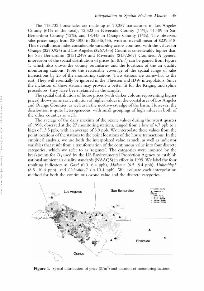
The 115,732 house sales are made up of 70,357 transactions in Los AngelesCounty (61% of the total), 12,523 in Riverside County (11%), 14,409 in SanBernardino County (12%), and 18,443 in Orange County (16%). The observedsales prices range from $20,000 to $5,345,455, with an overall mean of $239,518.This overall mean hides considerable variability across counties, with the values forOrange ($270,924) and Los Angeles ($267,455) Counties considerably higher thanfor San Bernardino ($151,249) and Riverside ($137,867) Counties. A generalimpression of the spatial distribution of prices (in $/m2) can be gained from Figure1, which also shows the county boundaries and the locations of the air qualitymonitoring stations. Note the reasonable coverage of the spatial range of salestransactions by 25 of the monitoring stations. Two stations are somewhat to theeast. They will essentially be ignored in the Thiessen and IDW interpolators. Sincethe inclusion of these stations may provide a better fit for the Kriging and splineprocedures, they have been retained in the sample.

The spatial distribution of house prices (with darker colours representing higherprices) shows some concentration of higher values in the coastal area of Los Angelesand Orange Counties, as well as in the north-west edge of the basin. However, thedistribution is quite heterogeneous, with small groupings of high values in both ofthe other counties as well.

The average of the daily maxima of the ozone values during the worst quarterof 1998, observed at the 27 monitoring stations, ranged from a low of 4.7 ppb to ahigh of 13.5 ppb, with an average of 8.9 ppb. We interpolate these values from thepoint locations of the stations to the point locations of the house transactions. In theempirical analysis, we use both the interpolated value as such, as well as indicatorvariables that result from a transformation of the continuous value into four discretecategories, which we refer to as ‘regimes’. The categories were inspired by thebreakpoints for O3 used by the US Environmental Protection Agency to establishnational ambient air quality standards (NAAQS) in effect in 1999. We label the fourresulting indicators as Good (0.0�6.4 ppb), Moderate (6.5�8.4 ppb), Unhealthy1(8.5�10.4 ppb), and Unhealthy2 (�/10.4 ppb). We evaluate each interpolationmethod for both the continuous ozone value and the discrete categories.

Figure 1. Spatial distribution of price ($/m2) and location of monitoring stations.



2.2. Econometric Issues

We estimate a hedonic function in log-linear form, with three types of explanatoryvariables: house-specific characteristics, neighbourhood characteristics (measured atthe census tract level), and air quality in the form of ozone (O3). We take anexplicit spatial econometric approach, which includes testing for the presence ofspatial autocorrelation and estimating specifications that incorporate spatialdependence. For a general overview of methodological issues involved in thespecification, estimation and diagnostic testing of spatial econometric models, werefer the reader to Anselin (1988), Anselin & Bera (1998), and, more recently,Anselin (2006). In this section, we limit our remarks to the specific test statistics andestimation methods employed in the empirical exercise. We refer the reader to theliterature for detailed technical treatments.4

We follow Anselin (1988) and distinguish between spatial dependence in aspecification that incorporates a spatially lagged dependent variable, and a modelwith a spatial autoregressive error term. We refer to these as spatial lag and spatialerror models. Formally, a spatial lag model is expressed as:

y�rWy�Xb�u; (1)

where y is an n�/1 vector of observations on the dependent variable, X is an n�/kmatrix of observations on explanatory variables, W is an n�/n spatial weightsmatrix, u an n�/1 vector of i.i.d. error terms, r is the spatial autoregressivecoefficient, and b a k�/1 vector of regression coefficients. A spatial error model is:

y�Xb�o (2)

o�lW o�u; (3)

where o is an n�/1 vector of spatial autoregressive error terms, with l as theautoregressive parameter, and the other notation is as in equation (1).

By means of the spatial weights matrix W , a neighbour set is specified for eachlocation. The positive elements wij of W are non-zero when observations i and jare neighbours , and zero otherwise. By convention, self-neighbours are excluded,such that the diagonal elements of W are zero. In addition, in practice, the weightsmatrix is typically row-standardized, such that ajwij �1: Many different definitionsof the neighbour relation are possible, and there is little formal guidance in thechoice of the ‘correct’ spatial weights.5 The term Wy in equation (1) is referred toas a spatially lagged dependent variable, or spatial lag. For a row-standardizedweights matrix, it consists of a weighted average of the values of y in neighbouringlocations, with weights wij .

In our application, we obtain the spatial weights matrix by first constructing aThiessen polygon tessellation for the house locations, which turns the spatialrepresentation of the sample from points into polygons. We next use simplecontiguity (common boundaries) as the criterion to define neighbours. Theresulting weights matrix is extremely sparse (0.005% non-zero weights) andcontains on average six neighbours for each location (ranging from a minimum of3 neighbours to a maximum of 35 neighbours for one observation). The weightsare used in row-standardized form.

For each model specification, we first obtain ordinary least squares (OLS)estimates and assess the presence of spatial autocorrelation using the LagrangeMultiplier test statistics for error and lag dependence (Anselin, 1988), as well as their



robust forms (Anselin et al ., 1996).6 The results consistently show very strongevidence of positive residual spatial autocorrelation, with a slight edge in favour ofthe spatial lag alternative (see Section 5). In addition to considering the estimates forthis specification, we also estimated the spatial error model, to further assess thesensitivity of the results to the way spatial effects are incorporated in the regression.

We use two types of estimation approaches. First, we apply the classical MLmethod (Ord, 1975; Anselin, 1988), but use the characteristic polynomial techniqueto allow the estimation in very large data sets (Smirnov & Anselin, 2001). We alsoexploit a sparse conjugate gradient method to obtain the inverse of the asymptoticinformation matrix (Smirnov, 2005). These estimation techniques and the regressiondiagnostics are carried out using GeoDa statistical software (Anselin et al ., 2006). Forthe spatial lag model, to avoid reliance on the assumption of Gaussian errors, we alsouse a robust estimation technique in the form of instrumental variables (IV)estimation, or spatial two-stage least squares (Anselin, 1988; Kelejian & Robinson,1993; Kelejian & Prucha, 1998). In addition, to account for the considerableremaining heteroskedasticity, we implement a heteroskedastically robust form ofspatial 2SLS, which is a special case of the recently suggested HAC estimator ofKelejian & Prucha (2005). Finally, for the spatial error model, we apply thegeneralized moments (GM) estimator of Kelejian and Prucha (1999), which does notrequire an assumption of Gaussian error terms. The robust estimation methods wereprogrammed as custom functions in R statistical software.

One final methodological note pertains to the assessment of model fit. In spatialmodels, the use of the standard R2 measure is no longer appropriate (see Anselin,1988, Ch. 14). When ML is used as the estimation method, a useful alternativemeasure is the value of the maximized log-likelihood, possibly adjusted for thenumber of parameters in the model in an Akaike Information Criterion (AIC) orother information criterion. However, for the models estimated by IV or GM,there is no corresponding measure. In order to provide for an informal comparisonof the fit of the various specifications, we also report a pseudo-R2, in the form ofthe squared correlation between observed and predicted values of the dependentvariable. In the classical linear regression model, this is equivalent to the R2, but inthe spatial models the use of this measure is purely informal and should beinterpreted with caution.

For the spatial error model, the pseudo-R2 is simply the squared correlationbetween y and y�Xb; where b is the estimated coefficient vector. However, inthe spatial lag model the situation is slightly more complex. Since the spatiallylagged dependent variable Wy is endogenous to the model, we obtain the predictedvalue from the expression for the conditional expectation of the reduced form:

y�E[yjX]� (I� rW )�1Xb: (4)

This operation requires the inverse of a matrix of dimension n�/n , which is clearlyimpractical in the current situation. We therefore approximate the inverse bymeans of a power method, which is accurate up to 6 decimals of precision.7

2.3. Remaining Issues

Our main focus is on the sensitivity of estimation results to the spatial interpolationmethod for the ozone measure. In order to keep this investigation tractable, thereare several methodological aspects that we control for and do not pursue at this



stage. These include a range of issues traditionally raised in the context of hedonicmodel estimation, such as the sensitivity of the results to functional form, variableselection, measurement error, identification, distributional assumptions, etc.

We include ozone as a single pollutant, given its visibility (as a major cause ofsmog) and extensive reporting in the popular media. We do not consider otherpotentially relevant criteria pollutants, such as particulate matter (PM2.5 and PM10).We use the same functional specification in all analyses, taking the dependentvariable in log-linear form and including the site-specific and neighbourhoodvariables used in the studies by Beron et al . (2001, 2004). We droppedneighbourhood variables that were consistently not significant (such as a crimeindicator). Arguably, more refined specifications could be considered, but this isrelevant in the current context only to the extent that these would affect theestimates of the spatially interpolated ozone values differentially, which is doubtful.

We also consider only one spatial weights matrix, which implies that anyinteraction effect between the properties of the spatial interpolation methods andthe specification of spatial weights has been ruled out. Since these are two verydifferent approaches to dealing with spatial effects (one based on discrete locationsand the other on a continuous surface), this seems a reasonable assumption.

More important is the potential effect of spatial heterogeneity, in the form ofcoefficient instability and the presence of spatial market segmentation. We leavethis as a topic for further investigation.8 Other potentially important methodolo-gical aspects that we do not consider at this time are the possible jointdetermination of location choice, house purchases and environmental quality.Apart from this source of endogeneity, there is also a potential errors in variablesproblem in the interpolated values. Since these values are treated as ‘observations’,any error associated with them is ignored. To the extent that such error patternsmay be correlated with the regression error, this may result in biased estimates(Anselin, 2001b).

We maintain that while these issues are important in and of themselves, they areless relevant in the current context, where the sensitivity to the differentinterpolation methods is our main concern. Our implicit assumption is thereforethat the relative performance of the interpolation methods will not be affected byignoring these other methodological aspects. We intend to investigate this furtherin future work.

3. Spatial Interpolation of Point Measures of Air Quality

In our empirical analysis, we need to allocate ozone measures obtained at thelocation of 27 monitoring stations to the locations of 115,732 sales transactions.This ‘point-to-point interpolation’ is the simplest among the change-of-supportproblems, and is well understood. The four techniques that we consider are readilyavailable in commercial GIS software, such as ESRI’s ArcGIS and its Spatial Analystand Geostatistical Analyst extensions.

Thiessen polygons or proximity polygons (also known as Delaunay triangulationor Voronoi diagrams) are obtained by assigning to each house the value measured atthe nearest monitoring station. This results in the partitioning of space into atessellation, which corresponds to the simple notion of a spatial market area in thesituation where only transportation costs matter.9 Consequently, the value forozone follows a step function, taking on only as many different values as observed atthe monitoring stations.



tesmith

Rectangle

Inverse distance weighting is a weighted average of the values observed at thedifferent monitors in the sample, with greater weight assigned to closer stations. Inpractice, due to the distance decay effect, the average only includes values observedfor a few nearest neighbours. Formally, the interpolated value at j is obtained as:

zj�P

i wiziP

i wi

; (5)

where the weights wi�1=f (dji) and f (dji) is a power of the distance between j andi . In our study, we set f (dji)�1=d2

ji :10

Kriging is an optimal linear predictor based on a variogram model of spatialautocorrelation. This is grounded in geostatistical theory and has an establishedtradition in natural resource modelling. A detailed discussion of the statisticalprinciples behind Kriging is beyond the scope of this paper, and we refer the readerto extensive treatments in Cressie (1993, Ch. 3), Burrough & McDonnell (1998,Ch. 6), and Schabenberger & Gotway (2005, Ch. 5), among others. In our study,we used ordinary Kriging (i.e. the interpolation was based on the ozone value itself,without additional explanatory variables in the model) and allowed for directionaleffects in a spherical model.11

Spline interpolators are based on fitting a surface through a set of points whileminimizing a smoothness functional, i.e. a function of the coordinates thatrepresents a continuous measure of fit subject to constraints on the curvature of thesurface. Parameters can be set to specify the ‘stiffness’ of the surface through atension parameter, which can be interpreted as a measure of the extent to whichany given point influences the fitted surface.12 We applied a regularized spline withthe weight set at 0.1.

4. Spatial Interpolation and Air Quality Regimes

We begin with a comparison of descriptive statistics for the ozone values assigned tothe house locations using each of the four interpolation procedures. Table 2summarizes the main results. While the overall averages for the four methods arevery similar, the large number of observations means that standard tests on equalityof means or medians strongly reject these null hypotheses.13

It is important to note the difference in variance between the interpolatedmeasures, as well as the different range. By design, both Thiessen and IDWmethods respect the range of the original observations (for the 27 monitoringstations), whereas the Kriging and spline methods do not. While the results forKriging stay within the observed range, the spline method yields interpolated values

Table 2. Descriptive statistics: interpolated ozone values

Thiessen IDW Kriging Spline

Mean 8.280 8.276 8.233 8.246

SD 2.033 1.906 1.912 1.967

Range 4.707� 13.467 4.707� 13.467 4.718� 13.464 4.543� 15.307

Correlation

Thiessen 1.0 0.980 0.933 0.939

IDW 1.0 0.965 0.960

Kriging 1.0 0.967



both below as well as above the observed range. Of the four methods, Thiessen hasthe highest overall average (8.28) and Kriging the lowest (8.23), while Thiessen alsohas the highest standard deviation (2.03), due to its being a step function rather thana continuous smoother. The non-spatial correlations between the four interpolatedvalues are extremely high, with the lowest observed between Thiessen and Kriging(0.933) and the highest between Thiessen and IDW (0.980).

The allocation of the interpolated values to the four categories of Good,Moderate, Unhealthy1 and Unhealthy2 is shown in Table 3. Interesting differencesoccur both at the low end and at the high end. In the best category, the largest shareis obtained for the Kriging method, with 23.6%, compared to values below 20% forthe others. The Thiessen method yields the largest share of houses in the worstgroup (20.5%), but when the two worst categories are taken together, the greatestshare is for Kriging (48.6%).

The resulting spatial distributions are quite distinct as well, as illustrated inFigures 2�5. Note in particular the qualitative difference between the edges ofregimes for the Thiessen and IDW interpolations, which are centred on themonitoring stations, and the much smoother patterns for Kriging and spline. Bothof these show roughly parallel zones of decreasing air quality moving away from thecoast. Also note the peculiar elliptical shape of the Good zone for the spline

Table 3. Observations by air quality regime

Thiessen IDW Kriging Spline

Good 20,191 19,363 27,368 19,649

17.5% 16.7% 23.6% 17.0%

Moderate 41,761 43,825 32,094 44,410

36.1% 37.9% 27.7% 38.4%

Unhealthy1 30,070 30,926 37,242 31,149

26.0% 26.7% 32.2% 26.9%

Unhealthy2 23,710 21,618 19,028 20,524

20.5% 18.7% 16.4% 17.7%

Figure 2. Spatial regimes for Thiessen interpolation.



interpolator, in contrast to a region that includes most of the coastal properties inLos Angeles County and north-west Orange County for Kriging.

5. Spatial Interpolation and Parameter Estimates in Hedonic Models

We start first with a broad overview of the results before focusing more specificallyon the estimates of the spatial coefficients and the parameters of the ozone variable.We estimated the hedonic model using six different methods with both acontinuous and discrete (regimes) ozone variable, and for each of the fourinterpolators, for a total of 48 specifications. The detailed results are not listed here,and only the salient characteristics are summarized.14

Figure 3. Spatial regimes for IDW interpolation.

Figure 4. Spatial regimes for Kriging interpolation.



tesmith

Line

The point of departure is the OLS estimation of the familiar log-linear hedonicmodel, which achieves a reasonable fit, ranging from an adjusted R2 of 0.769(Thiessen, continuous) to 0.774 (Kriging, regimes). For example, this fit iscomparable to the results reported in Beron et al . (2001), where the R2 valuesare around 0.70 but ours is a considerably larger dataset.

There is also strong evidence of very significant positive residual spatialautocorrelation, supported by both LM-Error and LM-Lag test statistics, with aslight edge in favour of the latter alternative.15 This is not surprising, given the finespatial grain at which we have observations on the sales transactions and the lack ofsuch spatial detail for the neighbourhood characteristics. If we maintain the spatiallag model as the proper alternative, the OLS estimates are biased and should beinterpreted with caution.

For each interpolator, and in both the continuous and discrete instances, thespatial lag specification obtains the best fit, and all spatial models fit the dataconsiderably better than the non-spatial OLS. This is a further indication that thelatter may yield biased estimates. To illustrate the improvement in fit, consider thebest interpolator, Kriging, for which the log-likelihood improves in the continuouscase from �/16,927 in the standard regression model to �/7,119 in the spatial lagmodel (the R2 value goes from 0.772 to a pseudo-R2 of 0.814). Similarimprovements are obtained for the other specifications.

Interestingly, the relative fit of the four interpolators is consistent across allestimation methods and for both the continuous and regimes ozone variable. Ineach case, Kriging is best, followed by spline and IDW, with Thiessen as worst.Also, in all but one instance (Thiessen, Lag-ML), the regimes model fits the databetter than the continuous one.

For OLS, the coefficient estimates for the house and neighbourhoodcharacteristics are significant and with the expected sign, except for Elevationand AC, which were both found to be negative. The Elevation coefficient may inpart capture an interaction effect with air quality, but the negative value forAC does not have an obvious explanation. The base case for the counties is

Figure 5. Spatial regimes for spline interpolation.



Los Angeles, with negative dummies in increasing order of absolute value forOrange, San Bernardino and Riverside.

The main difference between OLS and the spatial lag models lies in the absolutemagnitude of the estimates, with consistently much smaller values in the spatial lagspecification, as is to be expected. However, note that the OLS estimates may besuspect, given the strong indication in favour of the lag specification.16 The signsand significance are maintained for all but the coefficient of Income, whichbecomes negative in Lag-ML. However, this is only significant for Thiessen andIDW under ML estimation, but not for the other two methods. Also, thesignificance disappears for the IV and IV-Robust estimates (in the latter thecoefficient is positive, but not significant).

A closer look at the estimates for the spatial autoregressive parameter is providedin Table 4. All estimated coefficients are highly significant, with slightly highermagnitudes for the spatial autoregressive error parameter (but note that the spatialerror model is inferior in terms of fit relative to the spatial lag model). The spatialautoregressive lag coefficient ranges from 0.376 (Kriging, Lag-IV) to 0.446(Thiessen, Lag-ML). The largest estimates are consistently for the Thiesseninterpolator, and the smallest for Kriging. The ranking between estimationmethods is consistent as well, with the estimate for Lag-IVR between the higherLag-ML and the lower Lag-IV. As is to be expected, the estimated standard error islargest for the robust estimator. Relative to the continuous results, the Lag-MLestimates are smaller for the regimes models, but slightly larger for both IVestimators. However, when taking into account the standard errors of the estimates,there is little indication of a significant effect of the interpolator on the estimate ofthe spatial parameter. For example, consider the two estimates for the lag parameterusing IVR for Kriging�/2 standard errors, or, 0.3988�/0.0148�/0.4136 for

Table 4. Estimates for spatial autoregressive parametera

Model Thiessen IDW Kriging Spline

Continuous model

Lag-ML 0.4457 0.4438 0.4399 0.4428

(0.0030) (0.0030) (0.0030) (0.0030)

Lag-IV 0.3804 0.3791 0.3758 0.3786

(0.0052) (0.0052) (0.0052) (0.0052)

Lag-IVR 0.4054 0.4028 0.3988 0.4028

(0.0074) (0.0074) (0.0074) (0.0074)

Err-ML 0.5165 0.5139 0.5090 0.5130

(0.0036) (0.0036) (0.0036) (0.0036)

Err-GM 0.4653 0.4634 0.4599 0.4626

Regimes model

Lag-ML 0.4440 0.4404 0.4329 0.4348

(0.0031) (0.0031) (0.0031) (0.0031)

Lag-IV 0.3831 0.3808 0.3756 0.3786

(0.0052) (0.0052) (0.0052) (0.0052)

Lag-IVR 0.4142 0.4112 0.4039 0.4058

(0.0074) (0.0074) (0.0074) (0.0074)

Err-ML 0.5147 0.5102 0.4999 0.5035

(0.0036) (0.0036) (0.0037) (0.0037)

Err-GM 0.4632 0.4595 0.4524 0.4540

a Asymptotic standard errors are given in parentheses, except for the generalized moments method (l is a nuisance

parameter).



continuous ozone, and 0.4039�/0.0148�/0.4187 for the regimes. In each case, thepoint estimates for the other interpolators are included in this interval, suggestingthey do not differ significantly.

The situation is quite different for the ozone parameters, where we find adistinct and significant effect of the interpolator. The details are summarized inTable 5 for the continuous measure, and Table 6 for the regimes.

As shown in Table 5, all the estimates for the continuous ozone variable arehighly significant and have the expected negative sign. Relative to OLS andthe spatial error models, the absolute values are considerably smaller in the spatiallag model, for example, going from �/0.0270 for OLS Kriging to �/0.0179 forLag-ML Kriging. Interestingly, this is less the case for the Thiessen interpolator.The Kriging value is consistently the largest in absolute value, and exceeds theothers by more than 2 standard errors. The Thiessen value is consistently thesmallest in absolute value. IDW and spline are not significantly different from eachother and are in between these two extremes.

The differences between the interpolators are accentuated in the regimes results(Table 6). For OLS, the estimates for the Moderate category are counterintuitive,being positive and significant. This is also the case for the Unhealthy1 category usingthe Thiessen and IDW interpolators. In contrast, the corresponding estimates forKriging and spline are significant and negative. Only for the worst category(Unhealthy2) are the estimates negative across all interpolators, with the value forKriging significantly larger in absolute value than the others (again, with Thiessenyielding the smallest value). These results are essentially the same in the spatial errormodels, only with larger standard errors.

The main difference occurs for the spatial lag specifications. Here, the Kriginginterpolator yields results consistent with expectations. Even though the estimatefor Moderate is positive, it is not significant, and both Unhealthy categories arehighly significant and negative, with a larger absolute value for the worst category.The three other interpolators maintain a positive and significant value for Moderate .For Thiessen and IDW, Unhealthy1 is positive as well, although no longersignificant for the latter. Spline has negative and significant values for Unhealthy1 .

Overall, these results would suggest that the Kriging interpolator in a spatial lagspecification is the only one that yields estimates for a categorical air quality variable

Table 5. Estimates for ozone parameter (continuous model)a


OLS �/0.0126 �/0.0204 �/0.0270 �/0.0206

(0.0007) (0.0008) (0.0007) (0.0007)

Lag-ML �/0.0101 �/0.0148 �/0.0179 �/0.0139

(0.0006) (0.0007) (0.0006) (0.0006)

Lag-IV �/0.0105 �/0.0156 �/0.0192 �/0.0149

(0.0006) (0.0007) (0.0007) (0.0006)

Lag-IVR �/0.0101 �/0.0150 �/0.0187 �/0.0147

(0.0006) (0.0007) (0.0007) (0.0006)

Err-ML �/0.0120 �/0.0207 �/0.0277 �/0.0206

(0.0012) (0.0014) (0.0013) (0.0013)

Err-GM �/0.0121 �/0.0207 �/0.0276 �/0.0206

(0.0011) (0.0013) (0.0012) (0.0011)

a Asymptotic standard errors are given in parentheses.



consistent with expectations. This confirms earlier indications that this model alsoobtained the best fit.

6. The Valuation of Air Quality

We conclude this empirical exercise by comparing the valuation of air quality ascomputed from the parameter estimates for the different interpolators. Theorysuggests that the partial derivative of the hedonic price equation with respect to eachexplanatory variable yields its implicit price. Assuming that the housing market is inequilibrium, this can be interpreted as the marginal willingness to pay (MWTP) for anon-traded good such as air quality.17 Since our specification is log-linear, this yields:

MWTPz�@elnP

@z� bzP: (6)

Table 6. Estimates for ozone regime parametersa

Variable Thiessen IDW Kriging Spline

OLS Moderate 0.0528 0.0540 0.0310 0.0449

(0.0030) (0.0029) (0.0027) (0.0030)

Unhealthy1 0.0357 0.0230 �/0.0309 �/0.0051

(0.0029) (0.0029) (0.0026) (0.0029)

Unhealthy2 �/0.0365 �/0.0945 �/0.1761 �/0.1397

(0.0048) (0.0048) (0.0042) (0.0043)

Lag-ML Moderate 0.0140 0.0148 0.0006 0.0096

(0.0027) (0.0026) (0.0024) (0.0027)

Unhealthy1 0.0081 0.0007 �/0.0300 �/0.0152

(0.0026) (0.0026) (0.0024) (0.0026)

Unhealthy2 �/0.0432 �/0.0691 �/0.1161 �/0.0969

(0.0043) (0.0043) (0.0038) (0.0039)

Lag-IV Moderate 0.0194 0.0201 0.0046 0.0141

(0.0027) (0.0027) (0.0025) (0.0027)

Unhealthy1 0.0119 0.0037 �/0.0301 �/0.0139

(0.0026) (0.0027) (0.0024) (0.0026)

Unhealthy2 �/0.0423 �/0.0725 �/0.1241 �/0.1024

(0.0043) (0.0043) (0.0039) (0.0040)

Lag-IVR Moderate 0.0127 0.0142 0.0011 0.0094

(0.0030) (0.0030) (0.0026) (0.0028)

Unhealthy1 0.0096 0.0016 �/0.0292 �/0.0155

(0.0026) (0.0027) (0.0024) (0.0026)

Unhealthy2 �/0.0432 �/0.0727 �/0.1183 �/0.0995

(0.0039) (0.0040) (0.0037) (0.0037)

Err-ML Moderate 0.0544 0.0558 0.0342 0.0499

(0.0053) (0.0052) (0.0047) (0.0052)

Unhealthy1 0.0365 0.0229 �/0.0313 �/0.0044

(0.0052) (0.0053) (0.0047) (0.0051)

Unhealthy2 �/0.0251 �/0.0900 �/0.1764 �/0.1322

(0.0086) (0.0085) (0.0073) (0.0076)

Err-GM Moderate 0.0541 0.0556 0.0339 0.0488

(0.0048) (0.0048) (0.0044) (0.0048)

Unhealthy1 0.0363 0.0228 �/0.0314 �/0.0047

(0.0047) (0.0048) (0.0043) (0.0047)

Unhealthy2 �/0.0268 �/0.0907 �/0.1768 �/0.1339

(0.0079) (0.0078) (0.0068) (0.0070)

a Standard errors are given in parentheses.



In practice, this can be computed by using the average price for P . As shown in Kimet al . (2003, p. 35), the effect of the spatial multiplier in a spatial lag specification is tochange the MWTP to

MWTPz�@elnP

@z�

1

1 � rbzP; (7)

assuming a spatially uniform unit change, and with r as the estimate for the spatialautoregressive parameter.

We begin by comparing the ‘analytical’ MWTP estimates for each of theinterpolators between OLS and the spatial lag model that result from a 1 ppbdecrease in the value of the ozone variable. This change is assumed to applyuniformly throughout the sample and amounts, on average, to a 12% decrease. Forthe standard case (OLS), we apply equation (6), with a value of $239,518 for theaverage house price in the sample. The results are reported in Table 7, where boththe dollar amounts and the corresponding percentage of the house price are listed.Also, an approximate measure of the precision of the point estimate is given,obtained by computing the value for the parameter estimate 9/2 standard errors.For the spatial lag model we use equation (7), with the estimates for r; b and thecorresponding standard errors from the IVR method. Note that our reported‘standard errors’ in the spatial lag case are an underestimate of uncertainty, since thespatial parameter is assumed fixed (only the parameter values for ozone arechanged). This provides a reasonable approximation of the relative precision, butdoes not correspond to an analytical estimate of the overall standard error (e.g. asyielded by the delta method).

Before comparing the MWTP estimates between the non-spatial OLS resultsand the spatial lag model, note that the absolute value of the parameter estimate forozone in the latter is considerably smaller than for OLS. As illustrated in Table 7,this is more than compensated for by the spatial multiplier effect. In all instances,the estimated MWTP for the spatial lag model is considerably larger than for thematching OLS case.

There are also considerable differences between interpolators. The largestMWTP estimate is for Kriging in the spatial lag model. This value of $7,444exceeds that of all the other interpolators by some $1,500. In the OLS case also, theKriging estimate of $6,468 is much higher than the others. The smallest estimate isfor Thiessen, as low as $3,028 for OLS and $4,087 for the spatial lag model. In

Table 7. Analytical marginal willingness to pay, by interpolatora


OLS $3,028 $4,889 $6,468 $4,925

($2,699� 3,357) ($4,519� 5,241) ($6,127� 6,808) ($4,592� 5,258)

1.26% 2.04% 2.70% 2.06%

(1.13� 1.40%) (1.89� 2.19%) (2.56� 2.84%) (1.92� 2.20%)

Lag-IVR $4,087 $6,031 $7,444 $5,899

($3,609� 4,566) ($5,496� 6,567) ($6,920� 7,969) ($5,394� 6,404)

1.71% 2.52% 3.11% 2.46%

(1.51� 1.91%) (2.29� 2.74%) (2.89� 3.33%) (2.25� 2.67%)

a Uniform 1 ppb O3 improvement, assuming average house price. Two standard error bounds are given in

parentheses.



percentage terms, this ranges from 1.26% for Thiessen OLS to 3.11% for Krigingspatial lag.

The analytical approach breaks down for the categorical measures of air quality.Also, the uniform decrease of the ozone value throughout the sample does not fullyaccount for a possible differential effect of the interpolation methods. To assess thismore closely we introduce a simulation approach, based on re-interpolating valuesfrom the locations of the monitoring stations to the house locations. We lower thevalue observed at each station by 1 ppb and obtain new measures for each houselocation by interpolating. Note that, except for the Thiessen method, this does notresult in a uniform decrease for each house, since the interpolators are non-linear.Finally, we compute the predicted price for each house using the new ozone value(holding the other parameters and observed characteristics constant) and comparethis to the original sales price. In this process, we need to take account of the spatialmultiplier to obtain the predicted value in the spatial lag model. Since the change inthe variable is not uniform across space, the simplifying result used in equation (7)no longer holds. Instead, we must use the reduced form explicitly, as in equation(4). As before, we obtain an approximate measure of precision by carrying out thecalculation for the parameter value 9/2 standard errors.

In contrast to the analytical approach, this method can be used for both thecontinuous and categorical ozone models, since the newly interpolated ozone valuecan be reallocated to one of the four regimes. Also, since the predicted price iscomputed for each individual house, the results can be presented for any degree ofspatial aggregation.

The new relative distribution of observations that results from the allocation ofthe interpolated values to the four regimes is given in Table 8. This should becompared to the percentages in Table 3. The new interpolation results in a drasticshift of observations out of the Unhealthy2 category.

The simulated MWTP values for the continuous ozone model are reported inTable 9 as an average for the full sample. Relative to the analytical results (Table 7),the estimates are similar in magnitude, although uniformly somewhat smaller,ranging from a low of $2,895 for Thiessen OLS to a high of $6,961 for Krigingspatial lag. As before, the values differ greatly across interpolators, with Krigingyielding the highest estimates and Thiessen the lowest. Also, again the values aregreater for the spatial lag model relative to OLS, although to a lesser extent than inthe analytical approach.

A final assessment is presented in Table 10, where the estimated MWTP isgiven for both continuous and regimes models, and reported for the completesample as well as for each county. Two major features stand out. First, consideringthe totals only, the values for the regime models are clearly deficient in the OLScase, a direct result of the wrong signs obtained for the parameter estimates. Onlyfor the Kriging interpolator are they comparable to previous results.

Table 8. Reallocation of observations by air quality regime

Thiessen (%) IDW (%) Kriging (%) Spline (%)

Good 32.8 33.3 35.5 37.7

Moderate 41.3 40.7 38.6 37.2

Unhealthy1 22.0 23.9 23.6 22.6

Unhealthy2 3.9 2.0 2.3 2.4



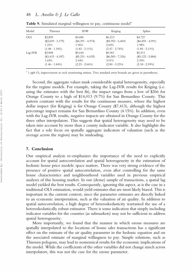
Second, the aggregate values mask considerable spatial heterogeneity, especiallyfor the regime models. For example, taking the Lag-IVR results for Kriging (i.e.using the estimates with the best fit), the impact ranges from a low of $266 forOrange County to a high of $14,013 (9.7%) for San Bernardino County. Thispattern contrasts with the results for the continuous measure, where the highestdollar impact (for Kriging) is for Orange County ($7,413), although the highestpercentage impact remains for San Bernardino County (4.15%). In addition, evenwith the Lag-IVR results, negative impacts are obtained in Orange County for thethree other interpolators. This suggests that spatial heterogeneity may need to betaken into account by more than a county indicator variable. It also highlights thefact that a sole focus on spatially aggregate indicators of valuation (such as theaverage across the region) may be misleading.

7. Conclusion

Our empirical analysis re-emphasizes the importance of the need to explicitlyaccount for spatial autocorrelation and spatial heterogeneity in the estimation ofhedonic house price models: space matters. There was very strong evidence of thepresence of positive spatial autocorrelation, even after controlling for the samehouse characteristics and neighbourhood variables used in previous empiricalanalyses of this housing market. In our (dense) sample of transactions, a spatial lagmodel yielded the best results. Consequently, ignoring this aspect, as is the case in atraditional OLS estimation, would yield estimates that are most likely biased. This isimportant in the current context, since the parameter estimates are directly linkedto an economic interpretation, such as the valuation of air quality. In addition tospatial autocorrelation, a high degree of heteroskedasticity warranted the use of aheteroskedastically robust estimator. There is some indication that simply includingindicator variables for the counties (as submarkets) may not be sufficient to addressspatial heterogeneity.

More importantly, we found that the manner in which ozone measures arespatially interpolated to the locations of house sales transactions has a significanteffect on the estimate of the air quality parameter in the hedonic equation and onthe associated estimate of marginal willingness to pay. Simple solutions, such asThiessen polygons, may lead to nonsensical results for the economic implications ofthe model. While the coefficients of the other variables did not change much acrossinterpolators, this was not the case for the ozone parameter.

Table 9. Simulated marginal willingness to pay, continuous modela


OLS $2,895 $4,686 $6,213 $4,727

($2,609� 3,175) ($4,391� 4,974) ($5,952� 6,469) ($4,455� 4,991)

1.21% 1.96% 2.60% 1.98%

(1.08� 1.34%) (1.82� 2.11%) (2.47� 2.74%) (1.85� 2.11%)

Lag-IVR $3,808 $5,640 $6,961 $5,511

($3,415� 4,187) ($5,231� 6,035) ($6,583� 7,326) ($5,122� 5,884)

1.65% 2.44% 3.01% 2.39%

(1.46� 1.84%) (2.23� 2.66%) (2.80� 3.23%) (2.18� 2.59%)

a 1 ppb O3 improvement at each monitoring station. Two standard error bounds are given in parentheses.



Of the four methods, the Kriging interpolator consistently yielded the best fit,as well as the most reasonable parameter signs and magnitudes, and related measuresof marginal willingness to pay. In addition, there was some indication that the useof categorical variables rather than a continuous ozone measure was superior. Inorder to deal with the lack of continuity of such variables, we employed asimulation method to estimate the change in house value associated with a decreasein ozone levels. This revealed the importance of spatial scale, and results at thecounty level that were vastly different from the regional aggregate.

Table 10. Simulated marginal willingness to pay, by countya

Model Region Thiessen IDW Kriging Spline

Continuous model

OLS All $2,895 $4,686 $6,213 $4,727

1.21% 1.96% 2.60% 1.98%

LA $2,980 $4,826 $6,422 $4,903

1.17% 1.89% 2.51% 1.92%

RI $2,211 $3,468 $4,401 $3,445

1.69% 2.65% 3.35% 2.63%

SB $2,399 $3,892 $5,178 $3,884

1.67% 2.71% 3.60% 2.70%

OR $3,429 $5,599 $7,457 $5,580

1.06% 1.74% 2.32% 1.73%

Lag-IVR All $3,808 $5,640 $6,961 $5,511

1.65% 2.44% 3.01% 2.39%

LA $4,012 $5,952 $7,375 $5,858

1.58% 2.34% 2.90% 2.30%

RI $3,018 $4,332 $5,112 $4,166

2.29% 3.28% 3.87% 3.16%

SB $3,246 $4,823 $5,972 $4,660

2.26% 3.36% 4.15% 3.25%

OR $4,000 $5,977 $7,413 $5,761

1.45% 2.16% 2.69% 2.08%

Regimes model

OLS All �/$311 $1,215 $5,103 $2,011

�/0.12% 0.51% 2.14% 0.84%

LA $18 $676 $4,604 $1,987

0.01% 0.26% 1.80% 0.78%

RI $7,669 $11,577 $11,129 $13,322

5.26% 8.83% 8.47% 10.16%

SB $8,335 $11,711 $13,879 $10,519

5.20% 8.15% 9.65% 7.31%

OR �/$13,735 �/$11,964 �/$3,943 �/$12,222

�/3.80% �/3.71% �/1.23% �/3.78%

Lag-IVR All $1,532 $2,858 $5,972 $4,010

0.66% 1.24% 2.59% 1.74%

LA $260 $1,074 $4,910 $2,822

0.10% 0.42% 1.93% 1.11%

RI $8,354 $12,382 $11,089 $13,861

6.34% 9.36% 8.37% 10.49%

SB $9,032 $12,465 $14,013 $10,997

6.28% 8.66% 9.74% 7.65%

OR �/$4,110 �/$4,314 $266 �/$3,610

�/1.49% �/1.57% 0.10% �/1.31%

a 1 ppb O3 improvement at each monitoring station, point estimates. Percentages are relative to the average house

price in each region.



While several methodological issues remain to be addressed, our findingssuggest that the quality of the spatial interpolation deserves the same type ofattention in the specification and estimation of hedonic house price models as moretraditional concerns. In future work, we intend to further investigate the role ofspatial heterogeneity and the potential endogeneity of the air quality measure.

Notes

1. For an extensive empirical assessment of spatial interpolation methods applied to ozone mapping, see, for

example, Phillips et al . (1997) and Diem (2003).

2. Other studies of the relation between house prices and air quality in this region can be found in Graves et al .

(1988) and Beron et al . (1999, 2001, 2004), although only Beron et al . (2004) takes an explicitly spatial

econometric approach. Also of interest is a general equilibrium analysis of ozone abatement in the same region,

using a hierarchical locational equilibrium model, outlined in Smith et al . (2004).

3. Owing to missing values, some stations had to be dropped from the complete set of stations available in the

region during that time period.

4. For recent collections reviewing the state of the art, see also Florax & van der Vlist (2003), Anselin et al .

(2004), Getis et al . (2004), LeSage et al . (2004), LeSage & Pace (2004) and Pace & LeSage (2004).

5. For a more extensive discussion, see Anselin (2002, pp. 256� 260), and Anselin (2006, pp. 909� 910).

6. See Anselin (2001a), for an extensive review of statistical issues.

7. This is implemented in the Python language-based PySAL library of spatial analytical routines; see http://

sal.uiuc.edu/projects_pysal.php

8. This is in addition to potential problems caused by the use of aggregate (census-tract level) variables in the

explanation of individual house prices (see Moulton, 1990).

9. For an extensive technical treatment of tessellations, see Okabe et al . (1992).

10. For further discussion of IDW, see, for example, Longley et al . (2001, pp. 296� 297).

11. The estimated parameter values were 302 and 7 for the direction (angle), 6 and 192 for the partial sill, 199,490

for the major range and 67,334 for the minor range. All Kriging interpolations were carried out with the ESRI

ArcGIS Geostatistical Analyst extension.

12. For a technical discussion, see, for example, Mitasova & Mitas (1993) and Mitas & Mitasova (1999).

13. The detailed results are not reported here, but available from the authors.

14. The detailed results are available from the authors and are included in an earlier Working Paper version.

15. The detailed test statistics are not reported, but are available from the authors. All test statistics are significant

with a p -value of less than 0.0000001 (the greatest precision reported by the software).

16. Since the spatial error model is consistently inferior in fit relative to the lag specification, we will not discuss it

in detail here. The main distinguishing characteristic of the findings is the difference in estimated standard

errors between OLS and the spatial error model. As a result, the coefficient of AC and of Poverty is no longer

significant in the spatial error model.

17. In addition to the equilibrium assumption, this interpretation is further complicated by the fact that the

estimated marginal benefits represent the capitalized rather than the annual value of the benefits of air quality

improvement. Therefore, other considerations, such as the length of time the buyer expects to reside in the

house, the discount rate and projected time path for air quality should all be taken into account (see also Kim

et al ., 2003, pp. 34� 37, for further discussion).

References

Anselin, L. (1988) Spatial Econometrics: Methods and Models, Dordrecht, Kluwer.

Anselin, L. (1998) GIS research infrastructure for spatial analysis of real estate markets, Journal of Housing Research ,

9(1), 113� 133.

Anselin, L. (2001a) Rao’s score test in spatial econometrics, Journal of Statistical Planning and Inference , 97, 113� 139.

Anselin, L. (2001b) Spatial effects in econometric practice in environmental and resource economics, American

Journal of Agricultural Economics , 83(3), 705� 710.

Anselin, L. (2002) Under the hood. Issues in the specification and interpretation of spatial regression models,

Agricultural Economics , 27(3), 247� 267.

Anselin, L. (2006) Spatial econometrics, in: T. Mills & K. Patterson (eds) Palgrave Handbook of Econometrics. Vol. 1:

Econometric Theory, pp. 901� 969, Basingstoke, Palgrave Macmillan.



Anselin, L. & Bera, A. (1998) Spatial dependence in linear regression models with an introduction to spatial

econometrics, in: A. Ullah & D. E. Giles (eds) Handbook of Applied Economic Statistics, pp. 237� 289, New York,

Marcel Dekker.

Anselin, L., Bera, A., Florax, R. J. & Yoon, M. (1996) Simple diagnostic tests for spatial dependence, Regional

Science and Urban Economics , 26, 77� 104.

Anselin, L., Florax, R. J. & Rey, S. J. (2004) Advances in Spatial Econometrics. Methodology, Tools and Applications,

Berlin, Springer.

Anselin, L., Syabri, I. & Kho, Y. (2006) GeoDa, an introduction to spatial data analysis, Geographical Analysis , 38,

5� 22.

Banerjee, S., Carlin, B. P. & Gelfand, A. E. (2004) Hierarchical Modeling and Analysis for Spatial Data, Boca Raton,

FL, Chapman & Hall/CRC.

Basu, S. & Thibodeau, T. G. (1998) Analysis of spatial autocorrelation in housing prices, Journal of Real Estate

Finance and Economics , 17, 61� 85.

Beron, K. J., Hanson, Y., Murdoch, J. C. & Thayer, M. A. (2004) Hedonic price functions and spatial dependence:

implications for the demand for urban air quality, in: L. Anselin, R. J. Florax & S. J. Rey (eds) Advances in Spatial

Econometrics: Methodology, Tools and Applications, pp. 267� 281, Berlin, Springer.

Beron, K. J., Murdoch, J. C. & Thayer, M. A. (1999) Hierarchical linear models with application to air pollution in

the South Coast Air Basin, American Journal of Agricultural Economics , 81, 1123� 1127.

Beron, K., Murdoch, J. & Thayer, M. (2001) The benefits of visibility improvement: new evidence from the Los

Angeles metropolitan area, Journal of Real Estate Finance and Economics , 22(2� 3), 319� 337.

Boyle, M. A. & Kiel, K. A. (2001) A survey of house price hedonic studies of the impact of environmental

externalities, Journal of Real Estate Literature , 9, 117� 144.

Brasington, D. M. & Hite, D. (2005) Demand for environmental quality: a spatial hedonic analysis, Regional Science

and Urban Economics , 35, 57� 82.

Burrough, P. A. & McDonnell, R. A. (1998) Principles of Geographical Information Systems, Oxford, Oxford

University Press.

Chattopadhyay, S. (1999) Estimating the demand for air quality: new evidence based on the Chicago housing

market, Land Economics , 75, 22� 38.

Chay, K. Y. & Greenstone, M. (2005) Does air quality matter? Evidence from the housing market, Journal of

Political Economy , 113(2), 376� 424.

Cressie, N. (1993) Statistics for Spatial Data, New York, John Wiley.

Diem, J. E. (2003) A critical examination of ozone mapping from a spatial-scale perspective, Environmental

Pollution , 125, 369� 383.

Dubin, R., Pace, R. K. & Thibodeau, T. G. (1999) Spatial autoregression techniques for real estate data, Journal of

Real Estate Literature , 7, 79� 95.

Florax, R. J. G. M. & van der Vlist, A. (2003) Spatial econometric data analysis: moving beyond traditional models,

International Regional Science Review , 26(3), 223� 243.

Freeman III, A. M. (2003) The Measurement of Environmental and Resource Values, Theory and Methods, 2nd edn,

Washington, DC, Resources for the Future Press.

Getis, A., Mur, J. & Zoller, H. G. (2004) Spatial Econometrics and Spatial Statistics, London, Palgrave Macmillan.

Gillen, K., Thibodeau, T. G. & Wachter, S. (2001) Anisotropic autocorrelation in house prices, Journal of Real

Estate Finance and Economics , 23(1), 5� 30.

Gotway, C. A. & Young, L. J. (2002) Combining incompatible spatial data, Journal of the American Statistical

Association , 97, 632� 648.

Graves, P., Murdoch, J. C., Thayer, M. A. & Waldman, D. (1988) The robustness of hedonic price estimation:

urban air quality, Land Economics , 64, 220� 233.

Harrison, D. & Rubinfeld, D. L. (1978) Hedonic housing prices and the demand for clean air, Journal of

Environmental Economics and Management , 5, 81� 102.

Kelejian, H. H. & Prucha, I. (1998) A generalized spatial two stage least squares procedures for estimating a spatial

autoregressive model with autoregressive disturbances, Journal of Real Estate Finance and Economics , 17, 99� 121.

Kelejian, H. H. & Prucha, I. (1999) A generalized moments estimator for the autoregressive parameter in a spatial

model, International Economic Review , 40, 509� 533.

Kelejian, H. H. & Prucha, I. R. (2005) HAC Estimation in a Spatial Framework , Working paper, Department of

Economics, University of Maryland, College Park, MD.

Kelejian, H. H. & Robinson, D. P. (1993) A suggested method of estimation for spatial interdependent models

with autocorrelated errors, and an application to a county expenditure model, Papers in Regional Science , 72,

297� 312.

Kim, C.-W., Phipps, T. T. & Anselin, L. (2003) Measuring the benefits of air quality improvement: a spatial

hedonic approach, Journal of Environmental Economics and Management , 45, 24� 39.



LeSage, J. P. & Pace, R. K. (2004) Advances in Econometrics: Spatial and Spatiotemporal Econometrics, Oxford, Elsevier

Science.

LeSage, J. P., Pace, R. K. & Tiefelsdorf, M. (2004) Methodological developments in spatial econometrics and

statistics, Geographical Analysis , 36, 87� 89.

Longley, P. A., Goodchild, M. F., Maguire, D. J. & Rhind, D. W. (2001) Geographic Information Systems and Science,

Chichester, John Wiley.

Mitas, L. & Mitasova, H. (1999) Spatial interpolation, in: P. A. Longley, M. F. Goodchild, D. J. Maguire & D. W.

Rhind (eds) Geographical Information Systems: Principles, Techniques, Management and Applications, pp. 481� 492,

New York, Wiley.

Mitasova, H. & Mitas, L. (1993) Interpolation by regularized spline with tension: I, theory and implementation,

Mathematical Geology , 25, 641� 655.

Moulton, B. R. (1990) An illustration of a pitfall in estimating the effects of aggregate variables on micro units,

Review of Economics and Statistics , 72, 334� 338.

Okabe, A., Boots, B. & Sugihara, K. (1992) Spatial Tessellations: Concepts and Applications of Voronoi Diagrams,

Chichester, John Wiley.

Ord, J. K. (1975) Estimation methods for models of spatial interaction, Journal of the American Statistical Association ,

70, 120� 126.

Pace, R. K., Barry, R. & Sirmans, C. (1998) Spatial statistics and real estate, Journal of Real Estate Finance and

Economics , 17, 5� 13.

Pace, R. K. & LeSage, J. P. (2004) Spatial statistics and real estate, Journal of Real Estate Finance and Economics , 29,

147� 148.

Palmquist, R. B. (1991) Hedonic methods, in: J. B. Braden & C. D. Kolstad (eds) Measuring the Demand for

Environmental Quality, pp. 77� 120, Amsterdam, North-Holland.

Palmquist, R. B. & Israngkura, A. (1999) Valuing air quality with hedonic and discrete choice models, American

Journal of Agricultural Economics , 81, 1128� 1133.

Phillips, D. L., Lee, E. H., Herstrom, A. A., Hogsett, W. E. & Tingey, D. T. (1997) Use of auxiliary data for spatial

interpolation of ozone exposure in southeastern forests, Environmetrics , 8, 43� 61.

Ridker, R. & Henning, J. (1967) The determinants of residential property values with special reference to air

pollution, Review of Economics and Statistics , 49, 246� 257.

Schabenberger, O. & Gotway, C. A. (2005) Statistical Methods for Spatial Data Analysis, Boca Raton, FL, Chapman

& Hall/CRC.

Smirnov, O. (2005) Computation of the information matrix for models with spatial interaction on a lattice, Journal

of Computational and Graphical Statistics , 14, 910� 927.

Smirnov, O. & Anselin, L. (2001) Fast maximum likelihood estimation of very large spatial autoregressive models:

a characteristic polynomial approach, Computational Statistics and Data Analysis , 35, 301� 319.

Smith, V. K. & Huang, J.-C. (1993) Hedonic models and air pollution: 25 years and counting, Environmental and

Resource Economics , 3, 381� 394.

Smith, V. K. & Huang, J.-C. (1995) Can markets value air quality? A meta-analysis of hedonic property value

models, Journal of Political Economy , 103, 209� 227.

Smith, V. K., Sieg, H., Banzhaf, H. S. & Walsh, R. P. (2004) General equilibrium benefits for environmental

improvements: projected ozone reductions under EPA’s Prospective Analysis for the Los Angeles air basin,

Journal of Environmental Economics and Management , 47, 559� 584.

Zabel, J. & Kiel, K. (2000) Estimating the demand for air quality in four U.S. cities, Land Economics , 76, 174� 194.



interpolation of air quality measures in hedonic house … and spatial heterogeneity) using the...

Documents