interplay of porous media and fracture stimulation in

$: Interplay of porous media and fracture stimulation in$
University of North DakotaUND Scholarly Commons

Theses and Dissertations Theses, Dissertations, and Senior Projects

2015

Interplay of porous media and fracture stimulationin sedimentary enhanced geothermal systems : RedRiver Formation, Williston Basin, North DakotaCaitlyn M. HartigUniversity of North Dakota

Follow this and additional works at: https://commons.und.edu/theses

Part of the Geology Commons

This Thesis is brought to you for free and open access by the Theses, Dissertations, and Senior Projects at UND Scholarly Commons. It has beenaccepted for inclusion in Theses and Dissertations by an authorized administrator of UND Scholarly Commons. For more information, please [email protected].

Recommended CitationHartig, Caitlyn M., "Interplay of porous media and fracture stimulation in sedimentary enhanced geothermal systems : Red RiverFormation, Williston Basin, North Dakota" (2015). Theses and Dissertations. 128.https://commons.und.edu/theses/128

https://commons.und.edu?utm_source=commons.und.edu%2Ftheses%2F128&utm_medium=PDF&utm_campaign=PDFCoverPages

https://commons.und.edu/theses?utm_source=commons.und.edu%2Ftheses%2F128&utm_medium=PDF&utm_campaign=PDFCoverPages

https://commons.und.edu/etds?utm_source=commons.und.edu%2Ftheses%2F128&utm_medium=PDF&utm_campaign=PDFCoverPages

https://commons.und.edu/theses?utm_source=commons.und.edu%2Ftheses%2F128&utm_medium=PDF&utm_campaign=PDFCoverPages

http://network.bepress.com/hgg/discipline/156?utm_source=commons.und.edu%2Ftheses%2F128&utm_medium=PDF&utm_campaign=PDFCoverPages

https://commons.und.edu/theses/128?utm_source=commons.und.edu%2Ftheses%2F128&utm_medium=PDF&utm_campaign=PDFCoverPages

mailto:[email protected]

INTERPLAY OF POROUS MEDIA AND FRACTURE STIMULATION IN

SEDIMENTARY ENHANCED GEOTHERMAL SYSTEMS: RED RIVER FORMATION,

WILLISTON BASIN, NORTH DAKOTA

by

Caitlin M. Hartig

Bachelor of Science, Pennsylvania State University, 2013

Bachelor of Musical Arts, Pennsylvania State University, 2013

Geographic Information Systems (GIS) Certificate, University of North Dakota, 2014

A Thesis

Submitted to the Graduate Faculty

of the

University of North Dakota

in partial fulfillment of the requirements

for the degree of

Master of Science

Grand Forks, North Dakota

May

2015

ii

iii

PERMISSION

Title Interplay of Porous Media and Fracture Stimulation in Sedimentary Enhanced

Geothermal Systems: Red River Formation, Williston Basin, North Dakota

Department Geology

Degree Master of Science

In presenting this thesis in partial fulfillment of the requirements for a graduate

degree from the University of North Dakota, I agree that the library of this University shall

make it freely available for inspection. I further agree that permission for extensive copying

for scholarly purposes may be granted by the professor who supervised my thesis work or, in

his absence, by the Chairperson of the department or the dean of the School of Graduate

Studies. It is understood that any copying or publication or other use of this thesis or part

thereof for financial gain shall not be allowed without my written permission. It is also

understood that due recognition shall be given to me and to the University of North Dakota in

any scholarly use which may be made of any material in my thesis.

Caitlin M. Hartig

4 May 2015

iv

TABLE OF CONTENTS

LIST OF FIGURES ....................................................................................................... vi

LIST OF TABLES ......................................................................................................... viii

ACKNOWLEDGEMENTS ........................................................................................... ix

ABSTRACT ................................................................................................................... x

CHAPTER

I. INTRODUCTION TO THE RESEARCH PROBLEM 1

Executive Summary .......................................................................... 1

Background to Geothermal and SEGS ............................................. 1

Research Area ................................................................................... 3

Research Site ..................................................................................... 5

Economics ......................................................................................... 9

Hypothesis ........................................................................................ 10

Research Objectives .......................................................................... 11

Deliverables ...................................................................................... 11

II. RED RIVER FORMATION INTRINSIC PROPERTIES 12

Research Question ............................................................................ 12

GIS Interpolations ............................................................................. 13

Discussion ......................................................................................... 26

Conclusion ........................................................................................ 27

v

III. RED RIVER FORMATION NATURAL FRACTURE ANALYSIS 29

Natural Fracture Data ....................................................................... 29

Stress Regime and Natural Fracture Orientation .............................. 29

Surface Lineament Orientation ......................................................... 33

Research Question ............................................................................ 34

GIS and Geostatistical Analysis ....................................................... 35

Discussion ......................................................................................... 40

Conclusion ........................................................................................ 40

DFN For Reservoir Simulation Modeling ........................................ 43

IV. FUTURE RESEARCH 47

Reservoir Simulation Modeling Objectives ...................................... 47

Location of SEGS ............................................................................. 47

Modeling Deliverable ....................................................................... 48

V. CONCLUSION 49

Potential Obstacles ............................................................................ 49

Revisiting the Hypothesis ................................................................. 51

Overall Project Benefits .................................................................... 51

APPENDIX .....................................................................................................................

REFERENCES ................................................................................................................

52

60

vi

LIST OF FIGURES

Figure Page

1. Nesson Anticline Area, Williston Basin .................................................................... 4

2. TSTRAT Plot for NDGS 5086 .................................................................................. 6



5. Red River Formation of the Williston Basin ............................................................. 12

6. Depth to Red River Formation Top ........................................................................... 14

7. Depth to Red River Formation Bottom ...................................................................... 14

8. Permeability of the Red River Formation .................................................................. 17

9. Porosity of the Red River Formation ......................................................................... 17

10. Surface Heat Flow of North Dakota .......................................................................... 19

11. Temperature of the Red River Formation (BHT) ...................................................... 19

12. Geothermal Gradient of the Red River Formation .................................................... 21

13. Heat Flow of the Red River Formation ..................................................................... 21

14. Temperature of the Red River Formation (Ordinary Kriging) .................................. 22

15. Moran’s I Analysis of the Calculated Temperatures ................................................. 23

16. Depth to the Top of the Formation on Temperature (OLS) ....................................... 24

17. The Effect of Heat Flow on Temperature (OLS) ....................................................... 24

18. Temperature of the Red River Formation (Co-Kriging) ............................................ 25

vii

Figure Page

19. Basement Faults and Surface Lineaments ................................................................. 36

20. Moran’s I Analysis of the Basement Faults ............................................................... 37

21. Moran’s I Analysis of the Surface Lineaments .......................................................... 37

22. Compass Plot of Basement Fault Trends ................................................................... 38

23. Compass Plot of Surface Lineament Trends .............................................................. 38

24. Compass Plot of the Basement Fault Trends and the Surface Lineament Trends ..... 39

25. Figure 24, Zoomed In ................................................................................................ 39

26. Lineaments as Fault Traces ........................................................................................ 42

27. Basement Faults ......................................................................................................... 44

28. Surface Lineaments .................................................................................................... 44

29. Basement Faults and Surface Lineaments ................................................................. 45

30. Areas of SEGS Interest .............................................................................................. 46

31. Hydrostratigraphy of the Williston Basin .................................................................. 49

viii

LIST OF TABLES

Table Page

1. North Dakota Stratigraphic Column Maximum Thicknesses and NDGS Well

5086 TSTRAT ...........................................................................................................

53

2. Red River Formation Depth, Thickness, Permeability, and Porosity ........................

54

3. NDGS Well 6840: Temperature, Thermal Conductivity, Depth, Thickness, and

HMC ..........................................................................................................................

56

4. Red River Formation BHTs, Geothermal Gradient, Heat Flow, and Predicted

Temperatures ............................................................................................................. 57

ix

ACKNOWLEDGEMENTS

First and foremost, I would like to sincerely thank all members of my advisory

committee for their instruction and guidance with this project. I express my heartfelt

gratitude to Dr. William Gosnold, Dr. Hadi Jabbari, and Dr. Richard LeFever for all of their

assistance.

I am indebted to Fred Anderson and Elroy Kadrmas for their GIS shapefile of

digitized surface lineaments over the Williston 250k in North Dakota. Without this file, my

geostatistical analysis of the natural fracture orientation would have been infeasible.

Furthermore, I would like to express my gratitude to my GIS professors for all of

their invaluable advice. I am grateful to Dr. Gregory Vandeberg, Dr. Michael Niedzielski,

and Dr. Enru Wang for all of their assistance.

I would like to sincerely thank Anna Crowell, Faye Ricker, Josh Crowell, Bailey

Bubach, and Dylan Young-- my colleagues on the UND geothermal team-- for assisting me

with various aspects of this project. Furthermore, I am grateful to Grant Ferguson, Jacek

Scibek, Jamie Russell, and Earl Klug for their ideas and source material.

Moreover, I would like to extend a huge thank you to my friends for all of their moral

support. Charis Dalessio, Haijing Chen, Amber Sharkawy, and Lisa Huber, I could not have

done it without you.

Last but not least, thank you to my favorite Starbucks crew on 32nd Avenue South.

You guys are seriously the best.

x

ABSTRACT

Fracture stimulated enhanced geothermal systems (EGS) can be installed in both

crystalline rocks and sedimentary basins. The Red River Formation (Ordovician), which lies

between 3.6 and 4.2 km depth in the Williston Basin, is a viable site for installation of

sedimentary EGS (SEGS). SEGS is possible there because temperatures in the formation

surpass 140° Celsius and the permeability is 0.1-38 mD; fracture stimulation can be utilized

to improve performance. The main objectives of this project were 1) to determine the spatial

variation of the intrinsic properties of the Red River Formation across the study area, and 2)

to understand the natural fracture orientation/location in the subsurface of the study area.

Maps of the intrinsic properties of the Red River Formation-- including depth to the top of

the formation, depth to the bottom of the formation, porosity, heat flow, geothermal gradient,

and temperature-- were produced by the Kriging interpolation method in ArcGIS. A GIS and

geostatistical analysis was completed to show that there is a satisfactory correlative

relationship between the surface lineaments and the basement faults in the study area.

Consequently, the orientations and locations of the surface lineaments and basement faults

were combined in a shapefile to represent the area’s discrete fracture network. In the future,

the results of these two analyses can be utilized to create a reservoir simulation model of an

SEGS in the Red River Formation; the purpose of this model would be to ascertain the

thermal response of the reservoir to fracture stimulation.

1

CHAPTER I

INTRODUCTION TO THE RESEARCH PROBLEM

Executive Summary

Fracture stimulated enhanced geothermal systems (EGS) can be installed in both

crystalline rocks and sedimentary basins. The Red River Formation (Ordovician), which lies

between 3.6 and 4.2 km depth in the Williston Basin, is a viable site for installation of

sedimentary EGS (SEGS). SEGS is possible there because temperatures in the formation

surpass 140° Celsius and the permeability is 0.1-38 mD; fracture stimulation can be utilized

to improve performance. The main objectives of this project were 1) to determine the spatial

variation the Red River Formation intrinsic properties across the study area, and 2) to

understand the natural fracture orientation/location in the subsurface of the study area.

Background to Geothermal and SEGS

The geothermal industry is currently struggling due to the high upfront financial cost

of geothermal systems, which limits market viability. The high upfront cost comes from the

high risk that is associated with exploration, production, and well drilling of geothermal

systems. The high risk comes from a paucity of subsurface information. Consequently,

geothermal industry leaders disagree on which techniques are the most economically viable,

and therefore where to distribute funds.

While some organizations-- for instance the U.S. Department of Energy-- advocate

for fracture stimulated Enhanced Geothermal Systems (EGS) installation in crystalline rocks,

other geothermal experts, such as David Blackwell, Paul Morgan, and Tom Anderson,

2

advocate for EGS in sedimentary basins (Blackwell et al., 2006; Morgan, 2013; Anderson,

2013). Sedimentary reservoirs have an edge over crystalline reservoirs when it comes to EGS

because even a small amount of the sedimentary basin's higher intrinsic permeability will

increase the efficiency of heat extraction (Tester et al., 2006). Furthermore, SEGS is

attractive because it utilizes existing oil field data; because of this, general knowledge of the

formation properties is improved and the cost of drilling is accordingly lowered.

In addition to having an edge over crystalline EGS, SEGS has an edge over

conventional sedimentary geothermal systems in the deeper formations of the basin. This

advantage is due to the fact that the rocks at the base of sedimentary basins (at depths greater

than 3 km) are similar in permeability and porosity to those in the basement (Tester et al.,

2006), with porosity about 20% and permeability about 25 mD. Therefore, it is actually

necessary to hydroshear the lower formations of sedimentary basins in order to improve the

permeability there, such that geothermal heat extraction would be feasible.

Moreover, many of the drawbacks that are associated with heat extraction from both

crystalline EGS and conventional sedimentary geothermal systems are reduced in an SEGS.

The main drawbacks of crystalline EGS include: 1) low permeability between the injection

and production wells, 2) difficulty in extracting sufficiently hot temperatures near the Earth’s

surface, i.e. requires deep drilling, and 3) limited lifespan of the system (Anderson, 2013).

The main drawback of sedimentary geothermal systems is that only low temperatures can be

extracted from the potential reservoirs (Anderson, 2013). In an SEGS, on the other hand, the

rock units have a higher permeability between the injection and production wells, moderate

temperatures (~150° C) can be extracted in the upper 4-5 km of the crust, and the system can

potentially be sustainable.

3

There are few SEGS currently on-line. A successful low-to-intermediate-temperature

binary unit project was previously successful in Maguarichic, Mexico (Blodgett, 2010) but is

no longer functional. In Germany, there are three main SEGS installed: Unterhaching,

Landau, and Horstberg. Unterhaching and Landau currently produce electricity with

cascaded heat, and Landau and Horstberg have demonstrated success with use of hydraulic

fracturing on low permeability sedimentary rocks (Morgan, 2013).

In the United States, an SEGS went on-line in Desert Peak, Nevada, in 2013. The

SEGS has already proven to be successful with its 175-fold increase in injectivity in the

target formation, use of cost-effective techniques and technologies, and effective approach to

multi-phase stimulation (Chabora and Zemach, 2013). The addition of fracture stimulation to

the Desert Peak reservoir resulted in a 38% increase in productivity (“Geothermal energy Hot

rocks,” 2014).

Several other SEGS projects have been considered for development in the United

States, but so far only Desert Peak has been implemented. Some of the sedimentary basins

that are candidates for SEGS installation include the Anadarko, Bighorn, Denver, East Texas,

Ft. Worth, Green River, Great Bain, Hannah, Delaware, Northern Louisiana, Powder River,

Raton, Sacramento, San Joaquin, Uinta, Williston, and Wind River basins (Porro and

Augustine, 2014; Blackwell et al., 2006). Because existing binary plants for moderate

temperature (150° C) SEGS have already proven to be successful, SEGS in the Williston

Basin within the Red River Formation, where temperatures are comparable, should be viable.

Research Area

As a result of its prominent geothermal potential and interconnectedness in a discrete

fracture network, the Williston Basin was selected as a potential candidate for SEGS

4

installation. A 60.0 km by 14.7 km (882 km2) section of the basin beneath the Nesson

Anticline in western North Dakota-- surrounding the junction of Divide, Burke, Williams,

and Mountrail counties-- was designated as the specific study area for this project (Figure 1).

In addition to having a large amount of thermal energy in place, the Williston Basin

has good reservoir productivity. There is an estimated 3.4*1019 KJ of thermal energy in place

in the Williston Basin, including both the rock and the pore fluids (Porro and Augustine,

2014). In order for a reservoir to be classified as having “great” reservoir productivity, there

should be high flow

volumes, vertical

permeability, strong

hydrothermal

recharge, and a well-

known thermal

profile (Porro and

Augustine, 2014).

Because it meets

most of these

standards, the

Williston Basin has

been classified as

ranging from “great to good” reservoir productivity (Porro and Augustine, 2014).

The reservoir productivity is greatly improved by the presence of a discrete fracture

network in the subsurface. The existing stress field in the Williston Basin is such that natural

Figure 1: Nesson Anticline Area, Williston Basin (William Gosnold, Pers. Comm., 2013).

5

stress fractures form from overpressure and interconnect as a result of tight spacing (Freisatz,

1995). This interconnectivity in the subsurface facilitates geothermal heat extraction because

there is a medium of travel available for the injected SEGS fluids.

Research Site

The Red River Formation (Ordovician) has been identified as a potential target for

installation of SEGS in the Williston Basin as a result of its oil production history, intrinsic

rock properties, and temperature. Because Red River Units B and C have been tapped for oil

production, there is sufficient data and information available about the formation on the

North Dakota Oil and Gas Division website (https://www.dmr.nd.gov/oilgas/) that can be

utilized for analysis.

Furthermore, the Red River Formation has porosity and permeability that are

conducive for SEGS installation because the lithology consists mostly of limestones and

dolostones (Tanguay and Friedman, 2001). The limestones are mainly composed of calcite

and contain minor amounts of dolostone, anhydrite, quartz, and halite (Tanguay and

Friedman, 2001). The dolostones are mainly composed of dolomite and calcite and contain

traces of quartz, anhydrite, and halite (Tanguay and Friedman, 2001). While the porosity and

permeability are “very low to low” in the limestones, porosity and permeability are “low to

moderate” in the dolostones (porosity of 10-24% and permeability of <1-62.8 mD,

respectively) (Tanguay and Friedman, 2001). Because the porosity and permeability are low

to moderate, the Red River Formation is a candidate for SEGS installation.

The temperature of the Red River Formation was initially determined from bottom-

hole temperature (BHT) data from the North Dakota Oil and Gas Division Website. These

BHT were measured from an instrument that recorded the temperature directly at the bottom

6

of the wellbore (Richard LeFever, Pers. Comm., 2015). Because BHTs are seldom measured

when the wellbore is at thermal equilibrium with the surrounding rock mass, it is necessary to

correct the temperatures to improve the accuracy of the measurements (Blackwell and

Richards, 2004a; Crowell and Gosnold, 2011; Crowell et al., 2011).

In spite of this, BHT measurements are still fairly unreliable predictors of subsurface

temperature after correction, Figures 2-4 (William Gosnold, Pers. Comm., 2015) show that

even corrected BHTs do not follow the standard temperature/depth profile for the earth’s

crust as predicted from the constant heat flow and depth of the stratigraphy for the NDGS

wellbores (obtained from the North Dakota Oil and Gas Division website). Corrected

temperatures still tend to underestimate the temperatures, particularly for depths greater than

2.5 km.

Because of the erratic nature of BHT measurements, a second method was

subsequently utilized to refine the corrected BHTs of the Red River Formation to improve

Figure 2: TSTRAT Plot for NDGS 5086 (William Gosnold, Pers. Comm., 2015).

7



8

the accuracy of the measurements. This method for obtaining formation temperatures has

been applied in previous regional and detailed assessments of geothermal resources in

sedimentary basins (Gosnold, 1984; Gosnold, 1991; Gosnold, 1999; Gosnold et al., 2010;

Crowell and Gosnold, 2011; Crowell et al., 2011; Gosnold et al., 2012) and in the

Geothermal Map of North America (Blackwell and Richards, 2004b). The assumptions of

this method are that 1) heat flow is conductive and constant, and 2) the geothermal gradient

varies inversely with thermal conductivity according to Fourier’s Law:

𝑞 = 𝑑𝑇

𝑑𝑧𝜆 (1)

where q is heat flow (mW/m2), 𝑑𝑇

𝑑𝑧 is the geothermal gradient (°C/m), and λ is thermal

conductivity (W/mK). Using this method, Red River Formation BHTs were input as

geothermal gradients into Equation 1 in order to obtain the heat flow. Once the heat flow had

been obtained for each well, the results were then input into Equation 2 in order to calculate

the subsurface temperature at each location:

𝑇(𝑧) = 𝑇0 + ∑𝑞𝑧𝑖

𝜆𝑖

𝑛

𝑖=1 (2)

where T(z) is temperature at depth z (°C), T0 is surface temperature (°C), q is heat flow

(mW/m2), zi is formation thickness (m) and λi is the formation thermal conductivity (W/mK).

Upon examining the Root Mean Square Error (RMSE) of the maps generated for both

the corrected temperatures and the calculated temperatures, the RMSE is lower for the map

of the calculated temperatures. Consequently, calculation is a more accurate method of

temperature prediction than is BHT correction alone. As a result of this analysis,

temperatures in the Red River Formation were found to surpass 140° C; therefore, the

reservoir temperature is sufficiently high for heat extraction using SEGS.

9

Economics

It is currently difficult to compare the cost of geothermal heat extraction to the cost

oil and gas extraction. Currently, few wells exist that are deeper than 2750 m (Tester et al.,

2006). To ameliorate this problem, the MIT Depth Dependent drilling index was developed

and used to normalize the predicted and actual completed geothermal well costs prior to

2004, such that they can be compared to oil and gas well costs (Tester et al., 2006).

There are a few differences in well design between geothermal wells and oil and gas

wells. Oil and gas wells typically use 6 3/4” or 6 1/4” bits; furthermore, they are lined with 4

1/2” or 5” casing that is almost always cemented in place and then shot perforated. On the

other hand, (vertical) geothermal wells are usually completed with 10 3/4” or 8 1/2” bits;

they are lined with 9 5/8” or 7” casing that is generally slotted or perforated instead of

cemented (Tester et al., 2006). Therefore, most (vertical) geothermal wells are two to five

times more expensive than oil and gas wells due to the higher cost of larger completion

diameters (Tester et al., 2006). According to Continental Resources, horizontal geothermal

wells are typically cheaper than vertical geothermal wells because they are generally smaller,

around 4 1/2” (www.contres.com); as a result of this, horizontal geothermal wells may have

pricing that is comparable to oil and gas wells.

While oil and gas drilling is generally cheaper than geothermal drilling, the

economics within geothermal drilling are significantly better for EGS in sedimentary rocks

than for EGS in crystalline rocks due to the differences in rock type and required drilling

depth. The hard, abrasive crystalline rocks reduce the rate of drilling penetration as well as

bit life, thereby increasing both the need for trips and the nonrotating drilling costs for the

project (Tester et al., 2006). On the other hand, these problems are alleviated in softer

10

sedimentary rocks. Moreover, the depth to the heat source is less in sedimentary basins than

it is in crystalline rocks, with the exceptions of the Basin and Range province, the Cascade

Range, and the Pacific-North American plate boundary. Therefore, fewer resources are

needed to reach the heat source in sedimentary rocks; thus the project completion time will

be faster. Given this information, sedimentary EGS is considerably less expensive than

crystalline EGS, with an estimated 20% cost savings (Tester et al., 2006)

Furthermore, the drilling cost is influenced by the number of required casing

intervals, which increases with depth. For a geothermal well at 5 km depth, a 4-casing well

costs $7.0 million to drill, whereas a 5-casing well costs $8.3 million to drill (Tester et al.,

2006). For a geothermal well at 4-5 km depth, four or five casing intervals are needed (Tester

et al., 2006). Because the Red River Formation is relatively shallow, at 4.0 km depth, it is

likely that four casing intervals would be sufficient, thereby reducing the cost.

To sum up, the cost of vertical geothermal drilling is two to five times more

expensive than the cost of oil and gas drilling as a result of the larger completion diameters.

On the other hand, horizontal geothermal drilling may be more cost comparable. Within

geothermal drilling, heat extraction in sedimentary basins has significantly lower costs than

heat extraction in crystalline EGS because 1) the softer rocks facilitate drilling, 2) the depth

to the heat source is less, and 3) fewer casings are needed to complete the drilling.

Hypothesis

The hypothesis for this research project was that SEGS is feasible in the Red River

Formation of the Williston Basin. To test this hypothesis, subsurface temperatures were

examined, as well as the mechanism for fluid flow in the subsurface.

11

Research Objectives

The main objectives of this research project were 1) to determine the spatial variation

of the intrinsic properties of the Red River Formation across the study area, and 2) to

understand the natural fracture orientation and location in the subsurface of the study area.

By completing these two objectives, a reservoir simulation model of the study area can be

completed in order to investigate the potential of the Red River Formation as a site for SEGS

installation.

Research was completed in the University of North Dakota Geothermal Laboratory in

Grand Forks, North Dakota. The advisory committee consisted of Dr. William Gosnold

(geothermics, geophysics, and structural geology), Dr. Hadi Jabbari (reservoir engineering

and hydraulic fracturing), and Dr. Richard LeFever (sedimentology and stratigraphy).

Deliverables

Maps of the intrinsic properties of the Red River Formation-- including depth to the

top of the formation, depth to the bottom of the formation, porosity, heat flow, geothermal

gradient, and temperature-- were produced by the Kriging interpolation method in ArcGIS.

Furthermore, a GIS and geostatistical analysis was completed to show that there is a

satisfactory correlative relationship between the surface lineaments and the basement faults

in the study area. Consequently, the orientations and locations of the surface lineaments and

basement faults were combined in a shapefile to represent the area’s discrete fracture

network. In the future, the results of these two analyses can be utilized to create a reservoir

simulation model of an SEGS in the Red River Formation; the purpose of this model would

be to ascertain the thermal response of the reservoir to fracture stimulation.

12

CHAPTER II

RED RIVER FORMATION INTRINSIC PROPERTIES

Research Question

In order to determine the spatial variation of the intrinsic properties of the Red River

Formation over the study area (Figure 5), interpolations were completed in ArcGIS using

well data from the North Dakota Oil and Gas Division website. The following parameters

were interpolated: depth to the top of the formation, depth to the bottom of the formation,

permeability, porosity, heat flow, geothermal gradient, and temperature.

Figure 5: Red River Formation of the Williston Basin. Nesson Anticline Area is shown in green in western North Dakota.

13

GIS Interpolations

The majority of the interpolations for the Red River Formation were completed using

the Kriging method, with the exception of the permeability; the Inverse Distance Weighted

(IDW) method was used instead to interpolate the permeability because the data were scarce.

The Kriging method of interpolation uses a semivariogram to determine the spatial

autocorrelation between points. On the other hand, the IDW method of interpolation uses the

inverse of the distance from the sample point to the target location to calculate the

interpolated value at the sample point. Regardless of the method used, the interpolations with

the lowest Root Mean Square Error (RMSE) were selected as the best models.

For complete accuracy to be obtained using the Kriging method, there need to be 150

or more data points. While there were only 81 total wells in this study area, the Kriging

method was utilized anyway-- instead of the IDW method-- because the interpolations had

much lower RMSE than they did with the IDW method. While the general error was reduced

using the Kriging method, it should be noted that some artifacts were added incorrectly to the

Kriging interpolations where there were no wells.

Data for the depth to the top of the formation (81 wells) and depth to the bottom of

the formation (36 wells) were obtained from the North Dakota Oil and Gas Division website.

The interpolation for the depth to the top of the formation is shown in Figure 6. Initially, the

36 wells were interpolated for the depth to the bottom of the formation with the goal of

obtaining the depths for the remaining 45 wells from that map. However, this method failed

due to lack of data coverage on the top of the study area. Therefore, to calculate the depth to

the bottom of the formation for the remaining 45 wells, the average unit thickness for the Red

River Formation was calculated and added to the depth to the top of the formation.

14

Figure 7: Depth to Red River Formation Bottom. Interpolation was completed using the Ordinary Kriging method; RMSE = 0.03770293.

Figure 6: Depth to Red River Formation Top. Interpolation was completed using the Ordinary Kriging method; RMSE = 0.03387275.

15

To obtain the average unit thickness for the Red River Formation, the maximum

thickness of the Red River Formation (213 m) was acquired from the North Dakota

Geological Survey (NDGS) North Dakota Stratigraphic Column (Murphy et al., 2009). Next,

TSTRAT (Temperature based on Stratigraphy) for NDGS Well 5086 (similar to that in

Gosnold et al., 2012) was utilized to calculate a correction factor for the NDGS maximum

thickness of the Red River Formation because the sum of the maximum thicknesses for the

Williston Basin formations (6545 m) (Murphy et al., 2009) was greater than the TSTRAT

depth to the bottom of the basin (4740 m) (Table 1, Appendix A). NDGS Well 5086 was

used for this correction because 1) the well had similar formation depth and thickness to the

study area, and 2) the well extended to the bottom of the basin.

It should be noted that all TSTRAT wells contain depth information from the North

Dakota Oil and Gas Division website that has been extrapolated to reach the depth of the

Precambrian Basement rocks based on the average unit thicknesses for each formation. For

instance, NDGS Well 5086 only reaches the Red River Formation, but the depth of the

stratigraphic column was projected to reach the Precambrian Basement by adding the

maximum thicknesses of the Red River Formation and the Deadwood Formation (Murphy et

al., 2009) to the depth to the top of the Red River Formation.

The correction factor was calculated in Equation 3:

Correction =𝑧𝑏

∑ 𝑧𝑚𝑎𝑥 (3)

where zb is depth to the bottom of the basin (NDGS Well 5086 TSTRAT) and ∑ 𝑧𝑚𝑎𝑥 is the

sum of the maximum thicknesses for the Williston Basin formations (Murphy et al., 2009).

Correction =4740 𝑚

6545 𝑚

Correction = 0.72

16

Subsequently, the maximum thickness of the Red River Formation (213 m) (Murphy et al.,

2009) was multiplied by the correction factor of 0.72, which resulted in an average unit

thickness of 0.154 km for the Red River Formation in the study area.

Consequently, 0.154 km was added to the depth to the top of the formation for each

well in the study area to obtain an approximate depth to the bottom of the formation for the

remaining 45 wells in the study area. The interpolation for depth to the bottom of the

formation is shown in Figure 7. Along with the data for the depth to the top of the formation,

the data for the depth to the bottom of the formation are listed in Table 2 in Appendix A.

Permeability was obtained from core analyses in the well log files on the North

Dakota Oil and Gas Division website. Out of 81 total Red River Formation wells in the study

area, only three wells-- 4379, 6915, and 1385—contained permeability data for the Red River

Formation as a whole. In addition to permeability for the formation as a whole, wells 6915

and 4379 also contained permeability data specifically for Red River Formation Unit C. For

the rest of the wells in the study area, only 8 had permeability data; those 8 measurements

were all specifically for Red River Formation Unit C. Consequently, permeability of only

Red River Unit C was interpolated (Figure 8); there were only 10 total measurements.

Because the permeability was interpolated specifically for Unit C, porosity was also

interpolated specifically for Unit C for consistency. Porosity data of Unit C were ascertained

from the Compensated Neutron Density (CND) logs when available (North Dakota Oil and

Gas Division). When there was no CND log, the Borehole Compensated Sonic (BCS) log

was utilized (North Dakota Oil and Gas Division) to obtain ∆tlog, which was then input into

Equation 4 to calculate the porosity:

𝜑𝑠𝑜𝑛𝑖𝑐 = ∆𝑡𝑙𝑜𝑔− ∆𝑡𝑚𝑎

∆𝑡𝑓− ∆𝑡𝑚𝑎 (4)

17

Figure 9: Porosity of the Red River Formation. Interpolation for Unit C was completed using the Ordinary Kriging method; RMSE = 0.05687078.

Figure 8: Permeability of the Red River Formation. Interpolation for Unit C was completed using the Inverse Distance Weighted (IDW) method; RMSE = 13.71893.

18

where 𝜑𝑠𝑜𝑛𝑖𝑐 is porosity, ∆𝑡𝑓 is 185 (typical value for salt), ∆𝑡𝑚𝑎 is 43.5 (typical value for a

limestone/dolostone lithology), and ∆𝑡𝑙𝑜𝑔 is the result from the BCS log (Wyllie et al., 1958).

There were 66 porosity measurements in total. It was assumed that 1) the reservoir

had a normal porosity distribution and 2) the porosity measurements included porosity of

both the natural fractures and rock pores. The interpolation for porosity is shown in Figure 9.

Along with the permeability data, the porosity data are listed in Table 2 in Appendix A.

Initially, heat flow was obtained from the National Geothermal Data System (NGDS)

global heat flow spreadsheet. However, this dataset only provided 8 heat flow points that fell

within the study area, which was not conducive to accurate interpolation. Furthermore, after

the interpolation of surface heat flow was completed (Figure 10), a mistake in the data

became apparent. Thus the NGDS dataset was not utilized for the remainder of the project.

Instead, the heat flow was calculated as follows. Bottom hole temperatures (BHT) for

50 of the 81 wells from the North Dakota Oil and Gas Division website were adjusted using

the Harrison Correction (interpolation shown in Figure 11). Subsequently, the geothermal

gradient was calculated for those 50 wells assuming a surface temperature of 6° C

(interpolation shown in Figure 12). BHTs are listed in Table 4 in Appendix A.

Once the geothermal gradient was calculated, the heat flow of each well (50 wells

total) was calculated using Fourier’s Law (Equation 1). To use Fourier’s Law, the thermal

conductivity of the basin first needed to be ascertained. To calculate the thermal conductivity

of the basin, Equations 5 and 6 were applied to the TSTRAT for NDGS Well 6840 (similar

method to Gosnold et al., 2012), using the data from Table 3 in Appendix A. NDGS Well

6840 was used for this purpose because 1) the well had similar formation depth and thickness

in comparison to the study area, and 2) the data was available for all formations in the basin.

19

Figure 11: Temperature of the Red River Formation (BHT). Bottom hole temperatures were adjusted using the Harrison Correction. Interpolation was completed using the Ordinary Kriging method; RMSE = 10.13062.

Figure 10: Surface Heat Flow of North Dakota. Data points were obtained for the Nesson Anticline Area from the NGDS global heat flow spreadsheet. Interpolation was completed using the Ordinary Kriging method; RMSE = 0.908885.

20

First, the Harmonic Mean Conductivity (HMC) of each formation was obtained using

Equation 5:

𝐻𝑀𝐶 =𝑧

𝜆 (5)

where HMC is Harmonic Mean Conductivity of each formation (K/m), z is formation

thickness (m), and λ is formation thermal conductivity (W/mK). Thermal conductivities of

each formation were measured from core samples provided by the North Dakota Geological

Survey (NDGS) with a divided bar apparatus, and the stratigraphic section was constructed

from the North Dakota Oil and Gas Division website (William Gosnold, Pers. Comm., 2015).

Subsequently, Equation 6 was utilized to calculate the thermal conductivity of the

Williston Basin as a whole (λbasin):

𝜆𝑏𝑎𝑠𝑖𝑛 =∑ 𝑧

∑ 𝐻𝑀𝐶 (6)

λ𝑏𝑎𝑠𝑖𝑛 = 1.667 W/mK

where λbasin is thermal conductivity of the basin (W/mK), ∑ 𝑧 is the sum of all formation

thicknesses (m), and ∑ 𝐻𝑀𝐶 is the sum of all formation HMC. Once the thermal

conductivity of the basin had been computed, heat flow was then calculated using Equation

1. The geothermal gradients used for this calculation are listed in Table 4 in Appendix A.

Subsequently, the heat flow results were interpolated in Figure 13 (circles). 32 Red

River Formation wells did not have bottom hole temperatures available; because of this, heat

flow could not be calculated for those wells. To ameliorate this problem, heat flow for these

32 wells was predicted from the well placement on Figure 13 (triangles). The heat flow

measurements for all wells are listed in Table 4 in Appendix A.

Once the heat flow had been ascertained for all 81 wells in the study area, the results

were input into an Excel model of NDGS Well 2894 TSTRAT (method similar to Gosnold et

21

Figure 13: Heat Flow of the Red River Formation. Interpolation was completed using the Ordinary Kriging method; RMSE = 2.719738.

Figure 12: Geothermal Gradient of the Red River Formation. A surface temperature of 6° C was used. Interpolation was completed using the Ordinary Kriging method; RMSE = 1.622047.

22

Figure 14: Temperature of the Red River Formation (Ordinary Kriging). Temperatures were calculated using thermal properties of rocks in the basin and heat flow. Interpolation was completed with the Ordinary Kriging method; RMSE = 4.987412.

23

al., 2012) to calculate the temperature of the Red River Formation for all wells using

Equation 2. NDGS Well 2894 was used for this purpose because 1) the well had similar

formation depth and thickness in comparison to the study area, and 2) the data was available

for all formations in the basin. Before the depths to the Red River Formation in the study area

were input into the Excel model, they were divided by 3989 m-- the depth to the top of the

Red River Formation listed in NDGS Well 2894 TSTRAT-- to correct for the difference in

depth between the model and the wells in the study area. The resulting temperatures are listed

in Table 4 in Appendix A and the interpolation is shown in Figure 14.

Once temperature had been calculated for all Red River Formation wells, a Moran’s I

analysis was completed in order to confirm that the temperature data were clustered (Figure

15). A Moran’s I analysis is a geostatistical method used in ArcGIS to calculate the spatial

autocorrelation of a dataset in order to determine whether that dataset is random, dispersed,

or clustered. It was predicted

that the temperature data

would show clustering

because the depth to the top

of the formation and the heat

flow are both input

parameters that influence the

temperature in the subsurface,

as shown by Equation 2. The

fact that the temperature data

showed clustering in the Figure 15: Moran's I Analysis of the Calculated Temperatures shows that the data are clustered and are thus not likely to be the result of random chance.

24

Figure 16: Depth to the Top of the Formation on Temperature (OLS). Temperature is 4% dependent on depth to the top of the formation.

Figure 17: The Effect of Heat Flow on Temperature (OLS). Temperature is 75% dependent on heat flow.

25

Figure 18: Temperature of the Red River Formation (Co-Kriging). Temperatures were calculated using thermal properties of rocks in the basin and heat flow. Interpolation was completed with the Co-Kriging method utilizing heat flow; RMSE = 1.925584.

26

Moran’s I confirmed that the model was working correctly and that there were sufficient data

points to complete the analysis.

Subsequently, Ordinary Least Squares (OLS) regressions showed that the influence of

heat flow on the formation temperatures was more than 18 times stronger than the influence

of depth to the top of the formation on the formation temperatures. Figure 16 shows that

depth to the top of the formation only influences the formation temperature by 4%, while

Figure 17 shows that heat flow influences the formation temperatures by 75%. Consequently,

heat flow is a far more significant control on the formation temperatures than depth.

Based on these results, a Co-Kriging interpolation of temperature was completed with

heat flow and is shown in Figure 18. A Co-Kriging interpolation differs from an Ordinary

Kriging interpolation in that the Co-Kriging method calculates the semivariance of two

variables (one independent and one dependent), while the Ordinary Kriging interpolation

only calculates the semivariance of one variable. In this case, temperature was the dependent

variable and heat flow was the independent variable. The model calculated the formation

temperatures by considering the effects of heat flow at each well location.

Discussion

Upon examining the surface heat flow interpolation in Figure 10, it is apparent that

there is a faulty data point in the NGDS spreadsheet. A surface heat flow value of 72 mW/m2

cannot logically be found so close to a surface heat flow value of 47 mW/m2. Because the

surrounding heat flow values are much lower, the faulty point must be that with 72 mW/m2.

Additionally, the presence of bull’s-eyes in Figure 10 indicates that 8 data points are

too few to produce an accurate interpolation. The bull’s-eye problem is also apparent in the

27

permeability interpolation (Figure 8) (10 data points) and the corrected BHT interpolation

(Figure 11) (50 data points). Consequently, these three interpolations should not be utilized.

Furthermore, there is a hint of distortion (jagged edges) on the southeast and northeast

corners of the Co-Kriging interpolation of the temperature with heat flow (Figure 18). In

spite of this, there is not so much distortion present that the interpolation should be discarded.

Because the Co-Kriging result (Figure 18) has the lowest RMSE out of the three

temperature interpolations, it is a viable temperature prediction. The Ordinary Kriging of

calculated temperatures (Figure 14) has no distortion and is therefore also a viable

temperature prediction, despite having a higher RMSE by a factor of more than 2.5.

Because the interpolation of the bottom hole temperatures (Figure 11) has an RMSE

twice as high as the Ordinary Kriging interpolation, it is evident that calculation of

subsurface temperatures based on heat flow and thermal properties is a more effective

method than just simply correcting and interpolating BHTs.

Conclusion

GIS analysis has been completed to produce interpolations of depth to the top of the

formation, depth to the bottom of the formation, permeability, porosity, geothermal gradient,

heat flow, and temperature. The interpolations for depth to the top of the formation (Figure

6), depth to the bottom of the formation (Figure 7), porosity (Figure 9), geothermal gradient

(Figure 12), and heat flow (Figure 13) are all acceptable results for input into a reservoir

simulation model. All that can be said for permeability is that it varies from 0.1-38 mD in the

limestones; the interpolation was inadequate due to a scarcity of data. Both the interpolation

of the calculated temperatures (Figure 14) and the interpolation of calculated temperatures

28

with the influence of heat flow (Figure 18) are acceptable predictions for the subsurface

temperatures that can be utilized in a reservoir simulation model.

Upon examining both Figures 14 and 18, it is apparent that the hottest section of the

region is in the south-central part of the study area. According to Figure 14, temperatures of

150-156° C are found in the southeastern corner of the study area (extending from the eastern

edge of Williams County into western Mountrail County). This hot section extends 9.8 km

horizontally and 8.0 km vertically. According to Figure 18, temperatures of 150-156° C are

found in the southwestern and south-central part of the study area (contained within Williams

County). This hot section extends 13.6 km horizontally and 9.9 km vertically. Regardless of

which temperature map is utilized, the southeastern section of Williams County has the

hottest temperatures, and is therefore the best place to install an SEGS in the study area.

It should be noted that there may be some interference from glacial isostasy in the

region; therefore, all temperatures shown in Figures 14 and 18 may be up to 15° too warm.

Consequently, it can only be said with certainty that the hottest temperatures surpass 140° C.

29

CHAPTER III

RED RIVER FORMATION NATURAL FRACTURE ANALYSIS

Natural Fracture Data

To understand the natural fracture orientation and location in the Red River

Formation, existing data was first examined. Unfortunately, seismic data were unavailable

for this study and therefore could not be utilized. Additionally, core images only existed for a

mere four wells in the study area (North Dakota Oil and Gas Division). While the cores

showed where the natural fractures intersected the wells, they were unoriented; as a result of

this, it was impossible to ascertain the natural fracture orientation from the core images.

As a result of this paucity of data, it was necessary to utilize literary analyses of the

Williston Basin’s stress field orientation, known natural fracture orientations, and surface

lineament orientations to deduce the natural fracture orientation of the study area.

Stress Regime and Natural Fracture Orientation

Natural fracture orientation can be inferred from the regional stress field. The stable

interior of North America—including the central and eastern United States, most of Canada,

and most of the western Atlantic—has been classified into the Midplate stress province

(M.D. Zoback and M.L. Zoback, 1991). The Midplate stress province is characterized by a

compressive stress regime of strike-slip and reverse faulting in which SHmax > SV > SHmin in

the United States (primarily-strike slip faulting) and SHmax > SHmin > SV in Canada (primarily

reverse faulting) (M.D. Zoback and M.L. Zoback, 1991; M.L. Zoback and M.D. Zoback,

1989). The cause of this stress regime has been attributed the absolute plate motion of the

30

North American plate to the Southwest, as well as to the ridge-push motions from the Mid-

Atlantic ridge (Bell and Grasby, 2012; M.L. Zoback and M.D. Zoback, 1989).

M.D. Zoback and M.L. Zoback, 1991 and Bell and Grasby, 2012 came to the above

conclusions from analyzing well bore breakouts. Well bore breakouts are anisotropic cavities

that occur on opposite sides of a borehole wall when the well is distorted as a result of stress

(Bell and Grasby, 2012). The breakouts are oriented in the direction of SHmin, where the

elastic compressive stress concentration is the greatest (Zoback et al., 1985).

M.D. Zoback and M.L. Zoback, 1991 analyzed the well bore breakouts with an

ultrasonic borehole televiewer. A televiewer is a well-logging tool that contains a

magnetically orientated rotating piezoelectric transducer that emits and receives an ultrasonic

(~1 MHz) acoustic pulse that is reflected from the borehole wall at 600 times per revolution

(Zoback et al., 1985). The televiewer shows the fractures that intersect the well bores as a

function of azimuth and depth, based on the reflectivity of the well bore; the reflected pulse

is shown as brightness on a three-axis oscilloscope and yields an “unwrapped” image of the

well bore surface (Zoback et al., 1985). One well was analyzed near Auburn, New York and

showed a 6.5-m long zone of breakouts in the well bore centered at a depth of 1476.3 m in a

Paleozoic sandstone (Zoback et al., 1985). Another well was analyzed near Monticello, South

Carolina and showed a 7.5-m long zone of breakouts in the well bore centered at a depth of

794.5 m in a granite (Zoback et al., 1985). Other break outs were similarly analyzed in the

southeastern corner of Saskatchewan (M.L. Zoback and M.D. Zoback, 1989), which is ~100

kilometers away from the current study area in western North Dakota.

Bell and Grasby, 2012 analyzed the well bore breakouts with a 4-arm dipmeter

imagery log for Mesozoic and Paleozoic shales, limestones, and dolostones. A dipmeter is an

31

instrument that documents the cavities on opposite sides of the well bore in order to ensure

that the lateral elongation of the borehole was caused by stress caving (Bell and Grasby,

2012). A dipmeter works by recording the extensions of opposing pairs of pads, in addition

to the compass orientation of one of the pads (Bell and Grasby, 2012). One well analyzed

was in northern Alberta and showed twenty-three ~254.8-m thick breakout intervals in the

well bore that were centered at a depth of 3496.35 m (Bell and Grasby, 2012). Only ten

measurements total were available in western Canada (Bell and Grasby, 2012).

The results of both of the above well bore breakout analyses showed a maximum

horizontal stress (compression) (SHmax) oriented in the east/northeast direction and a

minimum horizontal stress (compression) (SHmin) oriented in the north/northwest direction

(M.D. Zoback and M.L. Zoback, 1991; Bell and Grasby, 2012). Because SHmax is oriented

northeast/southwest, the natural fracture orientation can be inferred to also be oriented

northeast/southwest.

In other studies, there is an opposing viewpoint that local stresses, rather than tectonic

movements, are responsible for the stress regime in the Williston Basin. These studies

propose that the Nesson Anticline was formed along reactivated basement block boundaries

in response to varying tectonic stresses and crustal flexure that occurred intermittently

throughout the Phanerozoic (LeFever et al., 1987; Freisatz, 1995; Laird and Folsom, 1956).

In essence, these studies suggest that the stress regime of the Williston Basin is extensional,

rather than compressional.

LeFever et al., 1987 examined structural relief plots and split the area of the Nesson

Anticline into nine distinct areas, each of which having its own independent structural

history. Episodes of alternating uplift and subsidence occurred in each of these blocks in

32

different intervals over the Phanerozoic (LeFever et al., 1987). Most of these areas

experienced the largest amount of uplift in the Devonian or in the Early Mississippian, while

a few of these areas did not experience the largest amount of uplift until the Pennsylvanian

(LeFever et al., 1987). These results agree with the ideas of Laird and Folsom, 1956, who

believe that the Nesson Anticline formed sometime in the late Ordovician and became more

active at the end of the Paleozoic.

Other studies have been completed in the Canadian Williston Basin in Saskatchewan

and Manitoba to determine the natural fracture orientation in the subsurface of the Williston

Basin. In the Torquay-Rocanville trend near the Weyburn oil field in southeast

Saskatchewan, the flow of oil has been determined to be in a preferential northeast-southwest

orientation (Chen et al., 2009). As a result, it is suggested that natural fractures in the area

have a dominant northeast-southwest orientation (Chen et al., 2009). Furthermore, a

carbonate aquifer in southern Manitoba (middle Ordovician to Devonian) shows two

dominant fracture orientations observed in bedrock exposures: northeast-southwest (020°-

040°), and northwest-southeast (110°-130°) (Chen et al., 2011) or the equivalent (290°-310°).

The northwest trending group (perpendicular to SHmax and parallel to SHmin) has a higher

fracture density, but consists of mostly healed or closed fractures (Chen et al., 2011). The

northeast trending group (parallel to SHmax) has a significantly higher permeability and is the

preferential fluid-flow pathway (Chen et al., 2011; Wegelin, 1987).

Fluid in the subsurface should theoretically flow preferentially in the direction of

maximum stress, regardless of whether that stress is horizontal or vertical. Because Chen et

al., 2011 and Wegelin, 1987 observed the subsurface fluid to flow in a preferential northeast

direction, it can be assumed that the direction of maximum stress in the subsurface is oriented

33

to the Northeast (a horizontal stress). As a result of this information, it can be deduced that

the direction of maximum horizontal stress (SHmax) is oriented to the Northeast and that SHmax

is greater than the vertical overburden stress (SV). These findings suggests that the stress of

the region is SHmax > SHmin > SV, a compressive regime, which is consistent with the results of

Bell and Grasby, 2012 and M.D. Zoback and M.L. Zoback, 1991. If the stress regime were

extensional, on the other hand, then SV > SHmax > SHmin (Zoback, 1989). Thus the stress field

of the United States craton is a compressive regime that is caused by the northeastern

movements of the North American plate and the spreading of the Mid-Atlantic ridge.

To sum up, the consistent findings of Chen et al. 2011, Wegelin, 1987, Bell and

Grasby, 2012, and M.D. Zoback and M.L. Zoback, 1991 show that the natural fractures in the

subsurface of the Williston Basin are oriented northeast and northwest and that the northeast

trending group is the conduit for fluid flow. This information is applicable to the natural

fracture orientation in the Nesson Anticline area of the basin in North Dakota.

Surface Lineament Orientation

In addition to the two directions of natural fractures obtained from the Canadian

studies, there are also two distinct surface lineament (joint) zones in the area that are

coincidentally also trending northeast and northwest. Northeast and northwest trending

lineaments have been observed across Winnipeg (Chen et al., 2011) as well as in the Nesson

Anticline area and Mountrail County, North Dakota (Anderson, 2011; Gerhard et al., 1987).

It has been argued that surface lineament orientation can reflect the orientation of the

basement faults in the subsurface, and therefore by extension can reflect the specific

orientations and locations of the natural fractures in the formation (Bell and Grasby, 2012;

Anderson, 2011; Penner, 2006; Freisatz, 1995; Freisatz, 1991; Gerhard et al., 1987). The

34

assumptions are 1) that the basement faults cut through the subsurface formation in question,

2) that the trends of the natural fractures in the subsurface are parallel to the trends of the

basement faults, and 3) that the surface lineaments are formed either a) by the motion of the

basement faults, or b) by the same source that formed the basement faults. It has also been

proposed that the surface lineaments are vertically connected to the basement faults as fault

traces (Anderson, 2011; Chen et al., 2011; Freisatz, 1995).

In spite of the similarities in trend between the basement faults and the surface

lineaments, advances and retreats of Pleistocene glacial till show “ridge and swale”

topography that is also nearly coincident with the inferred direction of preferred fracture

orientations (Chen et al., 2011; Gerhard et al., 1990). Furthermore, Cenozoic detrital

sedimentary rocks can mask the geologic expression of the basin (Gerhard et al., 1990).

Because of this, lineaments may not be able to adequately predict the orientations of the

subsurface features (Chen et al., 2011; Gerhard et al., 1990; Gerhard et al., 1987).

Research Question

A paucity of natural fracture orientation data in the subsurface impedes immediate

understanding of the natural fracture orientation of the study area in western North Dakota.

While there are many known surface lineaments in the area and some known basement

faults, it is disputed that the surface lineaments are, in actuality, caused by the basement

faults. Thus it is uncertain whether or not it can be said with confidence that the surface

lineaments reflect the orientations and locations of the natural fractures in the subsurface.

As a result of this uncertainty, it was necessary to conduct a GIS and geostatistical

analysis comparing the trends of the surface lineaments to the trends of the basement faults in

order to determine whether or not they are sufficiently correlated. In the event that a strong

35

spatial autocorrelation were found to exist between the trends of the surface lineaments and

the trends of the basement faults, the approximation of the specific natural fracture

orientations and locations in the Red River Formation would be greatly facilitated.

GIS and Geostatistical Analysis

To begin the GIS and geostatistical analysis, two distinct shapefiles were needed: one

containing the spatial distribution of the surface lineaments and the other containing the

spatial distribution of the subsurface basement faults. The first shapefile was spatially

referenced and digitized by Fred Anderson and Elroy Kadrmas, 2011; it contained the spatial

distributions of all historic surface lineaments in the Williston 250k from Cooley, 1983 and

other sources. Lineaments in this file were derived from four distinct sources: 1) previous

studies, 2) digital shaded relief data, 3) aerial imagery, and 4) LANDSAT data/imagery

(Anderson, 2008). The second shapefile was a diagram of basement faults in Mountrail

County, North Dakota (Anderson, 2011) that was georeferenced to a shapefile of Mountrail

County (United States Census, 2014) and digitized into a separate layer. The basement faults

have been identified from seismic data (Anderson, 2011).

Once the two distinct shapefiles were obtained and created, respectively, the linear

directional mean tool and the directional distribution tool were run on both layers in ArcGIS

(Figure 19). The surface lineaments trend in two distinct directions (northwest and

northeast); therefore, the results of the linear directional mean and the directional distribution

were not included on the map because they did not reflect both directional trends.

Subsequently, Moran’s I analyses (Figures 20-21) were run on the lineaments and the

faults. From the clustered results, it is unlikely that either the lineaments or the faults were

formed by random chance.

36

Next, the trends for each distinct surface lineament and each distinct basement fault

were obtained for the geostatistical analysis with the linear directional mean tool. Compass

plots were created in MATLAB to analyze the relationships between the basement fault

trends and the surface lineament trends (Figures 22-25). Finally, the results were compared to

determine whether the spatial autocorrelation was strong enough to argue common causality.

Figure 19: Basement Faults and Surface Lineaments. Shows features for Mountrail County, North Dakota, 2011.

37

Figure 20: Moran's I Analysis of the Basement Faults shows that the data are clustered; therefore it is unlikely that they are the result of random chance.

Figure 21: Moran's I Analysis of the Surface Lineaments shows that the data are clustered; therefore it is unlikely that they are the result of random chance.

38

Figure 23: Compass Plot of the Surface Lineament Trends shows two distinctive trends: 320° (NW) and 043° (NE). Lineament density is greater in the northwest direction.

Figure 22: Compass Plot of the Basement Fault Trends shows an average ENE trend. The fault density is greatest at 042°, which is coincident with the directional distribution calculated in Figure 19. The linear directional mean calculated in Figure 19 (green stars) is pictured at 073°.

042°

320° 043°

073°

39

Figure 24: Compass Plot of the Basement Fault Trends and the Surface Lineament Trends. The large magnitude of lineaments and the small magnitude of faults makes comparison difficult.

Figure 25: Figure 24, Zoomed In. The closer view facilitates comparison.

40

Discussion

The average azimuthal direction of all subsurface faults, 073° (Figures 19 and 22), is

exactly coincident with the direction parallel to the regional stress field, SHmax, which is

oriented ENE in this area. The clustering shown in the Moran’s I analysis for the faults

(Figure 20) is thus explained because the regional stress field likely caused the faults to form.

The compass plot of the surface lineaments in Figure 23 shows two distinct directions

of trend: 320° (NW) and 043° (NE). The lineaments thus formed in the directions parallel

both to SHmin and SHmax of the regional stress field, respectively. Furthermore, the azimuthal

direction of lineaments trending northeast (043°) (Figure 23) is almost exactly coincident

with the azimuthal direction of most subsurface faults (042°) (Figure 22). Therefore, the

clustering shown in the Moran’s I analysis for the lineaments (Figure 21) is thus explained

because the regional stress field likely caused the faults to form, and then the faults likely

caused the lineaments to form.

Conclusion

A dearth of available seismic data in western North Dakota and a lack of oriented

cores hindered the immediate understanding of the natural fracture network present in the

Red River Formation. As a result of this, studies in the Williston Basin of the regional stress

field, natural fracture orientation, and surface lineament trends provided guidance in

deducing the orientation and location of the natural fractures in the subsurface of the Red

River Formation. The GIS and geostatistical analysis of the surface lineaments and the

basement faults in Mountrail County, North Dakota, showed that there is sufficient spatial

autocorrelation between the surface lineaments and the basement faults. It can thus be argued

that the regional stress field caused the faults to form, and that the fault movements

subsequently caused both the natural fractures and the surface lineaments to form. Because

41

the stress field is consistent over the study area, it can be assumed that the same relationships

apply to the lineaments and faults in the adjacent Burke, Divide, and Williams counties.

As a result of this correlative relationship between the surface lineaments, basement

faults, and natural fractures, it can be assumed that the surface lineaments mimic the

underlying orientations and locations of both the basement faults and the natural fractures in

the subsurface. According to Anderson, 2011, there are four different types of relationships

between surface lineaments and basement faults: coincident, adjacent, bridging, and

extending; furthermore, the basement faults are assumed to be subvertical (+/- 6 degrees from

vertical) (William Gosnold, Richard LeFever, Fred Anderson, and Stephan Nordeng, Pers.

Comm., 2014). The geometry of these relationships is summarized in Figure 26.

In all four relationships shown in Figure 26, the lineament trends are coincident with

the fault trends. Therefore, due to lack of more exact information regarding the specific

natural fracture orientation and location in the subsurface, it can be assumed that the surface

lineaments and natural fractures are coincident in terms of orientation and location.

Consequently, the natural fractures in the study area will be assumed to trend in the same

directions as the surface lineaments: 320° (NW) and 043° (NE), on average.

In agreement with the ideas of Chen et al., 2011 and Wegelin, 1987, the natural

fracture density is significantly greater in the northwest direction (SHmin) than in the northeast

direction (Figure 23). On the other hand, the natural fractures trending to the Northeast

(SHmax) are fewer in number but will be the conduits for flow. Because of this, it was

suggested that the northeast trending fractures are more likely to remain open with the

addition of fracture stimulation (Chen et al., 2011). Therefore, the hydroshearing dilation axis

would be parallel to SHmax in the northeast direction (Bell and Grasby, 2012). Furthermore,

42

Figure 26: Lineaments as Fault Traces. Shows a coincident relationship, an adjacent relationship, a bridging relationship, and an extending relationship.

43

production wells for the SEGS should be placed northeast of the injection wells in order to

maximize fluid flow.

DFN for Reservoir Simulation Modeling

More maps were made to show the locations of the basement faults and surface

lineaments in the whole research area. Figure 27 shows the locations of known basement

faults in the study area. Faults labeled “certain” have been identified based on both

stratigraphic and seismic data, while faults labeled “probable” have only been identified from

seismic data. Figure 28 shows the locations of all known surface lineaments in the study area

and can be utilized, due to lack of better knowledge, as a proxy for the natural fractures in the

subsurface. Figure 29 combines Figures 27 and 28 to show all known basement faults and all

known surface lineaments in the study area; consequently, the shapefile displayed in Figure

29 can be utilized to represent the discrete fracture network (DFN) of the study area in a

reservoir simulation model.

Furthermore, it has been shown that higher overall production rates correlate to areas

of greater lineament density (Anderson, 2011). The greatest lineament density occurs in the

northeastern corner of Williams County, which has 25 lineaments per 84.9 km2 (0.94

lineaments/km2) (Figure 30). Because the lineament density is greatest in the northeastern

corner of Williams County, this part of the study area would be an ideal spot to test in a

reservoir simulation model for placement of the SEGS.

44

Figure 27: Basement Faults showcases known faults in or around the study area. “Certain” faults have been identified based on both stratigraphic and seismic data. “Probable” faults have only been identified based on seismic data.

Figure 28: Surface Lineaments showcases known lineaments in the study area.

45

Figure 29: Basement Faults and Surface Lineaments in the study area. Because the surface lineaments and basement faults are spatially autocorrelated, it can be assumed that the surface lineaments mimic the trends of the natural fracture network in the subsurface. Therefore, the shapefile shown in this map can be utilized in reservoir simulation modeling to represent the discrete fracture network of the study area.

46

Figure 30: Areas of SEGS Interest are shown based on lineament density. Blue rectangles that are 9.016 km by 9.417 km (84.9 km2) highlight a section of northeastern Williams County with 25 lineaments and a section of southeastern Williams County with 22 lineaments.

47

CHAPTER IV

FUTURE RESEARCH

Reservoir Simulation Modeling Objectives

A reservoir simulation model will be completed in the future to continue this

research. Chad Augustine and his team at NREL have begun the process of modeling the

reservoir using Computer Modelling Group (CMG) STARS Advanced Processes Thermal

Reservoir Simulator. The objectives of the reservoir simulation modeling will be 1) to

describe the process of hydroshearing design, 2) to emphasize critical design factors that

determine design effectiveness, and 3) to investigate the optimal treatment selection for an

SEGS in the Red River Formation. Moreover, an economic analysis of the SEGS system will

be conducted in order to evaluate the financial performance of different treatment scenarios.

Location of SEGS

The results of the GIS analyses can be input into a reservoir simulation model in

order to ascertain the response of the Red River Formation to SEGS and fracture stimulation.

The ideal location for an SEGS would be 1) where the temperature in the subsurface is the

hottest, and 2) where there is high natural fracture density. Ideally, the hottest temperatures in

the formation would need a medium of transport (natural fractures) to be conducive to good

fluid flow and system mechanics. One location to test for the SEGS placement should be the

south-central part of the study area (the southeastern part of Williams County) in order to tap

the hottest temperatures in the Red River Formation within the research area (Figures 14 and

18). A second location to test for the SEGS placement would be the central part of the study

48

area (the northeastern corner of Williams County) in order to obtain the best production

results from the greatest amount of lineaments (natural fractures) (Figure 30). While the

southeastern part of Williams County has 22 lineaments (natural fractures) per 84.9 km2

(0.259 lineaments/km2), the northeastern corner of Williams County has 25 lineaments

(natural fractures) per 84.9 km2 (0.294 lineaments/km2) (Figure 30). On the other hand, the

northeastern corner of Williams County has temperatures ten degrees colder than the

southeastern part of Williams County (Figures 14 and 18). Because the southeastern part of

Williams County has the hottest temperatures in the study area in addition to a high natural

fracture density, and because the northeastern corner of Williams County has the highest

natural fracture density in addition to the second hottest temperatures in the study area, both

areas should be investigated in the reservoir simulation model as potential sites for SEGS

installation.

Modeling Deliverable

Ultimately, the reservoir simulation modeling will have the deliverables of a thermal

recovery assessment of the sedimentary geothermal reservoir to be installed in the Red River

Formation utilizing hydroshearing. The thermal recovery assessment will be complete with

analysis of the fluid injection rate, amount, and pressure. Furthermore, the amount of spacing

between the injection and production wells will be determined. A financial analysis of the

thermal recovery assessment will be completed in order to determine whether an SEGS

would be beneficial to install in the Red River Formation. It is predicted that the cost of the

SEGS installation will be offset by high productivity from the reservoir.

49

CHAPTER V

CONCLUSION

Potential Obstacles

There are three potential obstacles to the realization of this project: 1) contamination

of potable drinking water, 2) formation of gypsum scale, and 3) accumulation of sufficient

water for SEGS operation. These problems are

addressed below.

Whenever fluids are injected into the

ground, a question is presented as to whether

or not the project will result in the

contamination of potable water. Currently,

potable drinking water in the Williston Basin is

pumped from the Fox Hills Formation in the

Upper Aquifer (Whitehead, 1996). The Red

River Formation, on the other hand, is located

much deeper, in the basal aquifer (Figure 31).

As a result of this, the Red River Formation is

too deep to be utilized for drinking water.

Furthermore, the Red River Formation water

consists of saline brine with a total dissolved

solid (TDS) concentration greater than 100,000 Figure 31: Hydrostratigraphy of the Williston Basin (Faye Ricker, Pers. Comm., 2015).

50

milligrams per liter (Whitehead, 1996). Therefore, even if water were to be extracted from

Red River Formation, the water extracted from it would not be potable. Finally, SEGS fluids

that would be injected into the Red River Formation could not contaminate the overlying

aquifers because the Red River Formation is directly overlain by the basal aquitard (Figure

31).

The next potential problem of this project is that anhydrite (CaSO₄) traces are found

in the Red River Formation limestones and dolostones. As a result of this, gypsum

(CaSO*2H2O) scale will accumulate and clog the formation when water is injected into the

reservoir in the SEGS. Because there are only traces of anhydrite in the formation, it is

unlikely that gypsum formation would be ubiquitous. Moreover, the gypsum formation

process could be impeded by periodically diluting the reservoir with fresh water (Crabtree,

1999). In the event that gypsum scale were to accumulate in spite of periodic dilution, the

scale could be removed with an acid treatment that contains a chelating agent, for instance

ethylenediamenetetra-acetic acid (EDTA). The chelating agent is necessary because the

sulfate scale is difficult to remove as a result of its low solubility in acid (Crabtree, 1999).

The final potential problem of this project is that many gallons of water are needed to

continuously operate an SEGS. The reason for this is that 1) water needs to be injected

continuously into the reservoir to extract heat, and 2) water needs to be injected periodically

into the reservoir to complete the hydroshearing process. Consequently, the SEGS would

need to be located near an abundant source of water. One possible water source is the

Missouri River, which flows along the southern boundaries of Williams and Mountrail

counties. Fortuitously, the southeastern part of Williams County, where temperatures in the

study area are hottest, is only 1.3 miles away from the Missouri River. Given this

51

information, the SEGS site should be located in the southeastern part of Williams County,

rather than in the northeastern corner of Williams County.

Revisiting the Hypothesis

Thus far, SEGS is feasible in the Red River Formation of the Williston Basin in

western North Dakota. In the proposed SEGS site in the southeastern part of Williams

County, temperature is sufficiently high (140° C) and porosity and permeability are high

enough (17% and 0.1-38 mD, respectively) to yield a large volume of fluid. The presence of

a DFN in the subsurface further facilitates flow.

Currently, there are no major problems that would impede the completion of a

successful project. However, once the results of the reservoir simulation modeling are

obtained, the hypothesis can either be fully supported or fully refuted with certainty.

Overall Project Benefits

This project will result in an overall improved knowledge of SEGS and of the existing

geothermal potential in the Red River Formation of the Williston Basin in western North

Dakota. This improved knowledge will consequently lower the drilling risk for the area. As a

result of the reduced drilling risk, there will be lower drilling and completions costs. As a

result of the lowered costs, the geothermal industry will flourish.

APPENDIX

53

APPENDIX A

List of Tables

Table 1. North Dakota Stratigraphic Column Maximum Thicknesses and NDGS Well 5086 TSTRAT

Formation Maximum Thickness* (m) Well 5086 Depth to Formation Top** (m)

Brule 61 382.5

Chadron 43

Golden Valley 122 438.75

Tongue R. 396

487.5 Slope Fm. 82

Cannonball Fm. 78

Ludlow 91

Hell Creek 101 937.5

Fox Hills 122 1087.5

Pierre 701 1177.5

Niobrara 76 1702.5

Carlisle 122 1758.75

Greenhorn 46 1848.75

Belle Fourche 107 1882.5

Mowry 91 1961.25

Newcastle 46 2002.5

Skull Creek 43 2036.25

Inyan Kara 191 2066.25

Swift 221 2227.5

Rierdon 30 2340

Piper 191 2362.5

Spearfish 229 2505

Minnekahta 21 2673.75

Opeche 152 2682.5

Broom Creek 114 2772.75

Amsden 137 2847.75

Tyler 82 2874

Otter 61 2934

Kibbey 76 2979

Charles 225

3035.25 Mission Canyon 303

Lodgepole 225

Bakken 49 3845.25

Three Forks 82 3511.5

Bird Bear 46 3567.75

Duperow 163 3597.75

Souris R. 114 3702.75

54

Table 1. cont.

Dawson Bay 58 3781.5

Prairie 198 3822.75

Winnepegosis 67 3972.75

Interlake 390 4062.75

Stonewall 37 4314

Stony Mountain 76 4340.25

Red River 213 4385.25

Winnipeg 161 4546.5

Deadwood 305 4640.25

PreCambrian -- 4740

Sum of Maximum

Thicknesses: 6545 --

*Murphy et al., 2009

**NDGS Well 5086 TSTRAT

Table 2. Red River Formation Depth, Thickness, Permeability, and Porosity

Well Depth to the

Top of the

Formation

(km)

Depth to the

Bottom of the

Formation

(km)

Thickness*

(km)

Permeability**

(mD)

∆tlog** Porosity**

(%)

32 3.91 4.09 0.180

235 3.84 4.00 0.154 11

355 3.83 4.01 0.184

1231 3.86 4.04 0.176

1385 4.00 4.20 0.197 6.2

1636 3.96 4.15 0.191

2009 3.84 3.99 0.154

3844 3.94 4.14 0.198 55 5

4321 3.88 4.06 0.184 4

4323 3.84 4.02 0.182 10

4340 4.07 4.22 0.154 50 2

4379 3.85 3.92 0.067 9.3 54 5

4390 3.85 4.00 0.154 25

4420 3.88 4.03 0.154 58 10

4434 3.88 4.03 0.154 55 5

4514 3.90 4.05 0.154

4665 3.81 3.97 0.154 53 7

4716 3.88 4.07 0.189 54 5

5069 3.92 4.12 0.192 5

5192 3.64 3.79 0.154 8

5197 3.87 4.02 0.154 9

5545 3.86 4.02 0.154

55

Table 2. cont.

5577 3.83 4.02 0.182 18

5612 3.86 4.02 0.154 19

5648 3.85 4.00 0.154 15

5656 3.87 4.02 0.154 0.5 15

5658 3.86 4.01 0.154

5725 3.87 4.06 0.189 19

5726 3.85 4.00 0.154 18

5912 3.90 4.09 0.192 25

5937 3.87 4.06 0.188 20

6029 3.89 4.04 0.154 21

6087 3.91 4.06 0.154 18

6098 4.05 4.26 0.208 18

6108 3.86 4.01 0.154 18

6111 3.88 4.04 0.154 21

6362 3.92 4.08 0.154 17

6545 3.81 3.91 0.101

6569 4.02 4.17 0.154 19

6915 4.12 4.21 0.090 0.1 11

7005 3.94 4.15 0.204 12

7557 3.87 4.03 0.154 20

7595 3.87 4.02 0.154 20

7856 3.80 3.96 0.154

8645 3.98 4.02 0.046 20

8689 3.95 4.05 0.104 11

8722 3.83 3.91 0.076 13

9207 3.82 3.97 0.154 13

9361 3.85 4.00 0.154 14

9642 3.85 3.99 0.142 19

9801 3.86 4.01 0.154 15

10073 3.84 4.00 0.154 22

10328 3.84 4.00 0.154 13

11089 3.89 4.04 0.154 0.535 13

11126 3.86 4.01 0.154 11

11164 3.85 4.00 0.154 10

11405 3.84 4.00 0.154 15

11760 4.13 4.18 0.054

12024 3.88 4.07 0.190 17

12035 3.76 3.92 0.154 16

12109 3.77 3.92 0.154 27

12119 3.83 4.00 0.173 1.08 10

56

Table 2. cont.

12261 3.74 3.90 0.154 14

12270 3.83 4.00 0.175 3 9

12290 3.80 3.95 0.154 14

12305 3.97 4.15 0.183 17

12329 3.75 3.90 0.154 15

12363 3.87 4.06 0.186 14

12366 3.78 3.93 0.154 14

12432 3.87 4.05 0.181 9

12556 3.93 4.08 0.154 22

12592 3.94 4.12 0.181 15

12597 3.91 4.10 0.191 14

12790 3.87 4.02 0.154 38

12906 3.65 3.80 0.154

12917 3.89 4.04 0.154 8

12971 4.00 4.20 0.197 19.9 23

13395 3.87 4.06 0.186 22.8 24

13682 3.91 4.09 0.184 12

15089 3.90 4.05 0.154 15

18680 3.93 4.14 0.204

*Thickness of 0.154 km refers to the average unit thickness value for the Red River Formation as calculated

from the maximum thickness of the Red River Formation from the NDGS North Dakota Stratigraphic Column

(Murphy et al., 2009) correlated to NDGS Well 5086 (in essence, the value from Murphy et al., 2009 corrected

by a factor of 0.72). The thickness of 0.154 km was utilized to calculate the depth to the bottom of the formation

for wells in which that depth was unavailable from the North Dakota Oil and Gas Division website.

**Measurements were obtained only for Red River Unit C.

Table 3. NDGS Well 6840: Temperature, Thermal Conductivity, Depth, Thickness, and HMC

Formation Temperature

(°C)

λ (W/mK) Depth (m) Thickness

(m)

Harmonic Mean

Conductivity (K/W)

Brule 6 1.2 49 49.41 41.18

Chadron 6 1 84 34.83 34.83

Golden Valley 6 1.4 183 98.82 70.59

Tongue R. 14.8 1.3 433 250 192.3

Slope 17.3 1.3 499 66.42 51.09

Hell Creek 20.3 1.3 581 81.81 62.93

Fox Hills 24.1 1.2 680 98.82 82.35

Pierre 47.2 1.2 1248 567.81 473.2

Niobrara 49.8 1.1 1309 61.56 55.96

Carlisle 54.2 1.2 1408 98.82 82.35

Greenhorn 54.8 1.1 1423 14.7 13.36

Belle Fourche 57.5 1.1 1484 61 55.45

Mowry 60.6 1.1 1555 71 64.55

Newcastle 62.6 1.5 1599 44 29.33

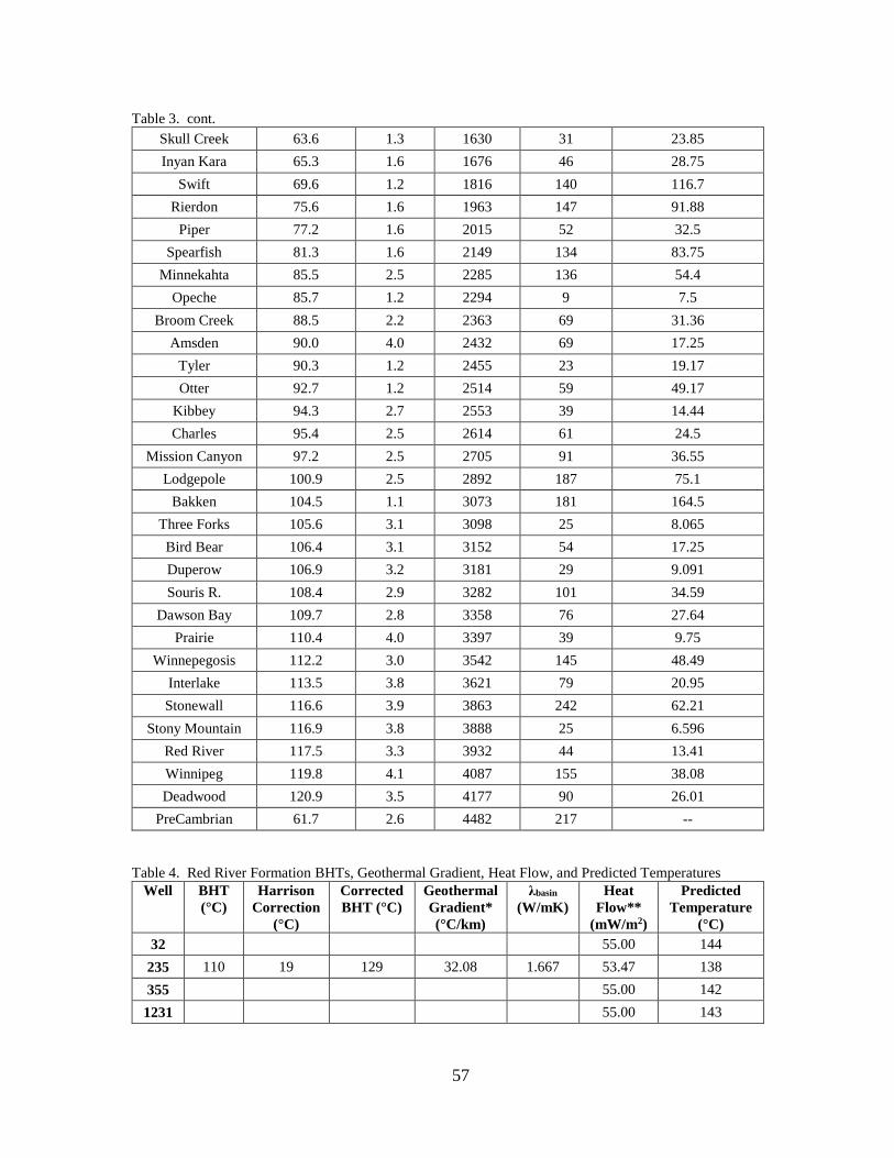
57

Table 3. cont.

Table 4. Red River Formation BHTs, Geothermal Gradient, Heat Flow, and Predicted Temperatures

Well BHT

(°C)

Harrison

Correction

(°C)

Corrected

BHT (°C)

Geothermal

Gradient*

(°C/km)

λbasin

(W/mK)

Heat

Flow**

(mW/m2)

Predicted

Temperature

(°C)

32 55.00 144

235 110 19 129 32.08 1.667 53.47 138

355 55.00 142

1231 55.00 143

Skull Creek 63.6 1.3 1630 31 23.85

Inyan Kara 65.3 1.6 1676 46 28.75

Swift 69.6 1.2 1816 140 116.7

Rierdon 75.6 1.6 1963 147 91.88

Piper 77.2 1.6 2015 52 32.5

Spearfish 81.3 1.6 2149 134 83.75

Minnekahta 85.5 2.5 2285 136 54.4

Opeche 85.7 1.2 2294 9 7.5

Broom Creek 88.5 2.2 2363 69 31.36

Amsden 90.0 4.0 2432 69 17.25

Tyler 90.3 1.2 2455 23 19.17

Otter 92.7 1.2 2514 59 49.17

Kibbey 94.3 2.7 2553 39 14.44

Charles 95.4 2.5 2614 61 24.5

Mission Canyon 97.2 2.5 2705 91 36.55

Lodgepole 100.9 2.5 2892 187 75.1

Bakken 104.5 1.1 3073 181 164.5

Three Forks 105.6 3.1 3098 25 8.065

Bird Bear 106.4 3.1 3152 54 17.25

Duperow 106.9 3.2 3181 29 9.091

Souris R. 108.4 2.9 3282 101 34.59

Dawson Bay 109.7 2.8 3358 76 27.64

Prairie 110.4 4.0 3397 39 9.75

Winnepegosis 112.2 3.0 3542 145 48.49

Interlake 113.5 3.8 3621 79 20.95

Stonewall 116.6 3.9 3863 242 62.21

Stony Mountain 116.9 3.8 3888 25 6.596

Red River 117.5 3.3 3932 44 13.41

Winnipeg 119.8 4.1 4087 155 38.08

Deadwood 120.9 3.5 4177 90 26.01

PreCambrian 61.7 2.6 4482 217 --

58

Table 4. cont.

1385 55.00 148

1636 55.00 146

2009 57.00 147

3844 55.00 145

4321 55.00 143

4323 55.00 142

4340 130 19 149 35.19 1.667 58.67 149

4379 55.00 142

4390 113 19 132 32.74 1.667 54.58 141

4420 118 19 137 33.81 1.667 56.36 146

4434 117 19 136 33.50 1.667 55.85 145

4514 116 19 135 33.19 1.667 55.32 145

4665 122 19 141 35.54 1.667 59.25 151

4716 55.00 143

5069 55.00 145

5192 110 19 129 33.81 1.667 56.37 138

5197 110 19 129 31.88 1.667 53.14 138

5545 55.00 143

5577 55.00 142

5612 126 19 145 35.95 1.667 59.92 155

5648 113 19 132 32.76 1.667 54.61 141

5656 113 19 133 32.74 1.667 54.58 142

5658 55.00 143

5725 55.00 143

5726 112 19 131 32.61 1.667 54.35 141

5912 55.00 144

5937 55.00 143

6029 110 19 129 31.72 1.667 52.88 138

6087 109 19 128 31.27 1.667 52.13 137

6098 57.00 154

6108 113 19 133 32.80 1.667 54.68 142

6111 119 19 139 34.17 1.667 56.96 148

6362 119 19 139 33.81 1.667 56.37 148

6545 57.00 146

6569 104 19 124 29.30 1.667 48.85 133

6915 118 19 137 31.90 1.667 53.18 147

7005 57.00 150

7557 121 19 140 34.56 1.667 57.61 149

7595 113 19 132 32.57 1.667 54.29 141

7856 57.00 145

59

Table 4. cont.

8645 106 19 125 29.87 1.667 49.79 134

8689 111 19 130 31.50 1.667 52.51 140

8722 121 19 140 35.08 1.667 58.48 150

9207 117 19 136 34.03 1.667 56.73 145

9361 112 19 131 32.45 1.667 54.10 140

9642 124 19 144 35.76 1.667 59.61 153

9801 112 19 131 32.51 1.667 54.19 141

10073 124 19 144 35.83 1.667 59.73 153

10328 109 19 128 31.78 1.667 52.98 137

11089 127 19 146 36.14 1.667 60.24 156

11126 109 19 128 31.64 1.667 52.74 137

11164 105 19 124 30.76 1.667 51.27 133

11405 128 19 147 36.69 1.667 61.15 157

11760 132 19 151 35.24 1.667 58.74 161

12024 55.00 144

12035 118 19 138 34.97 1.667 58.29 147

12109 118 19 137 34.78 1.667 57.98 146

12119 57.00 146

12261 114 19 134 34.12 1.667 56.87 143

12270 125 19 144 36.11 1.667 60.20 154

12290 118 19 137 34.49 1.667 57.49 146

12305 121 19 140 33.88 1.667 56.47 143

12329 112 19 131 33.47 1.667 55.79 141

12363 55.00 143

12366 114 19 134 33.81 1.667 56.36 143

12432 55.00 143

12556 116 19 135 32.80 1.667 54.68 144

12592 55.00 145

12597 127 19 146 35.77 1.667 59.62 156

12790 117 19 136 33.59 1.667 56.00 145

12906 114 19 133 34.80 1.667 58.02 142

12917 118 19 137 33.72 1.667 56.21 146

12971 55.00 148

13395 55.00 143

13682 55.00 144

15089 118 19 138 33.74 1.667 56.25 147

18680 55.00 145

*Geothermal gradient was calculated by subtracting a surface temperature of 6° C from the corrected BHT

and dividing that value by the depth to the top of the formation in km listed in Table 1.

**Heat flow for wells without BHT measurements was predicted from well placement in Figure 13.

60

REFERENCES

Anderson, Fred J., 2008, Lineament mapping and analysis in the northeastern Williston Basin

of North Dakota: North Dakota Geological Survey, Geological Investigations No. 70, p. 26.

Anderson, Fred J., 2011, Structural Relationships between Surface Lineaments and Basement

Faulting in the Northeastern Williston Basin: The Rocky Mountain Association of Geologists

(RMAG), p. 376-392.

Anderson, Fred J., and Kadrmas, Elroy, compilers, 2011, Shapefile of historic surface

lineaments in the Williston 250k.

Anderson, Tom C., 2013, Geothermal Potential of Deep Sedimentary Basins in the United

States, in GRC Transactions, A Global Resource, from Larderello to Las Vegas, Volume 37:

Davis, CA, Geothermal Resources Council, p. 223-229.

Bell, J.S., and Grasby, S.E., 2012, The stress regime of the Western Canadian Sedimentary

Basin, in Geofluids, Volume 12: p. 150-165.

Blackwell, David D., et al., 2006, Geothermal Resources in Sedimentary Basins: Southern

Methodist University.

Blackwell, D.D., and Richards, M., 2004a, Geothermal Map of North America Explanation

of Resources and Applications: Southern Methodist University.

Blackwell, D.D., and Richards, M., 2004b, Geothermal Map of North America: AAPG, scale

1:6,500,000, Product Code 423.

Blodgett, Leslie, 2010, Developing Geothermal Energy at Low Temps:

http://www.renewableenergyworld.com/rea/news/article/2010/09/low-t (accessed February

2014).

Chabora, Ethan, and Zemach, Ezra, 2013, Desert Peak EGS Project: U.S. Department of

Energy.

Chen, Zhuoheng, et al., 2009, Spatial variation of Bakken or Lodgepole oils in the Canadian

Williston Basin, in AAPG Bulletin, Volume 93, number 6: p. 829-851.

Chen, Zhuoheng, et al., 2011, Geologic controls on regional transmissivity anisotropy, in

Geofluids, Volume 11: p. 228-241.

61

Cooley, M. E., 1983, Linear features determined from LANDSAT imagery in North Dakota:

USGS Open File Report 83-937.

Crabtree, Mike, et al., 1999, Fighting Scale—Removal and Prevention: Oilfield Review, p.

30-45.

Crowell, Anna M., et al., 2011, GIS Analysis for the Volumes, and Available Energy of

Selected Reservoirs: Williston Basin, North Dakota., in GRC Transactions, A Global

Resource, from Larderello to Las Vegas, Volume 35: Davis, CA, Geothermal Resources

Council, p. 1581-1585.

Crowell, Anna M., and Gosnold, W.D., Jr., 2011, Correcting Bottom-Hole Temperatures: A

Look at the Permian Basin (Texas), Anadarko and Arkoma Basins (Oklahoma), and

Williston Basin (North Dakota), in GRC Transactions, A Global Resource, from Larderello

to Las Vegas, Volume 35: Davis, CA, Geothermal Resources Council, p. 735-738.

Freisatz, Wayne B., 1991, Fracture-enhanced Porosity and Permeability Trends in the

Bakken Formation, Williston Basin, Western North Dakota [Master’s thesis]: University of

North Dakota.

Freisatz, Wayne B., 1995, Fracture-enhanced Porosity and Permeability Trends in the

Bakken Formation, Williston Basin, Western North Dakota: Proceedings of Seventh

International Williston Basin Symposium.

Geothermal energy Hot rocks, 2014, in The Economist, p. 54-55.

Gerhard, L.C., et al., 1987, Structural History of the Nesson Anticline, North Dakota, in

Williston Basin: Anatomy of a Cratonic Oil Province, p. 337-354.

Gerhard, L.C., et al., 1990, Petroleum geology of the Williston Basin, in M.W. Leighton,

D.R. Kolata, D.F. Oltz, and J.J. Eidel, eds., Interior cratonic basins: AAPG Memoir, Volume

51: p. 509-559.

Gosnold, W.D., Jr., 1984, Geothermal Resources in the Williston Basin: North Dakota, in

GRC Transactions, A Global Resource, from Larderello to Las Vegas, Volume 8: p. 431-436.

Gosnold, W.D., Jr., 1991, Subsurface temperatures in the northern Great Plains, in

Slemmons, D.B., Engdahl, E. R., Zoback, M.D., and Blackwell, D.D., eds., Neotectonics of

North America: Boulder, Colorado, Geological Society of America, Decade Map Volume I:

p. 467-472.

Gosnold, W.D., Jr., 1999, Basin-Scale groundwater flow and advective heat flow: An

example from the northern Great Plains, in Forster and Merriam, eds., Geothermics in Basin

Analysis: Kluwer Academic/Plenum, p. 99-116.

62

Gosnold, W.D., Jr., et al., 2010, EGS Potential in the Northern Midcontinent of North

America, in GRC Transactions, A Global Resource, from Larderello to Las Vegas, Volume

34: Davis, CA, Geothermal Resources Council.

Gosnold, W.D., Jr., et al., 2012, Thermostratigraphy of the Williston Basin, in GRC

Transactions, A Global Resource, from Larderello to Las Vegas, Volume 36: Davis, CA,

Geothermal Resources Council.

Laird, W. M., and Folsom, C. B., Jr., 1956, North Dakota's Nesson anticline: North Dakota

Geological Survey Report of Investigation 22, 12 p.

LeFever, Julie A., et al., 1987, Structural evolution of the central and southern portions of the

Nesson Anticline, North Dakota: Proceedings of Fifth International Williston Basin

Symposium, p. 147-156.

LeFever, Richard, 2014, Shapefile of basement faults in the Williston Basin, Nesson

Anticline Area.

Morgan, Paul, 2013, Advantages of Choosing a Sedimentary Basin as the Site for an EGS

Field Laboratory, in GRC Transactions, A Global Resource, from Larderello to Las Vegas,

Volume 37: Davis, CA, Geothermal Resources Council, p. 179-183.

Murphy et al., 2009, North Dakota Stratigraphic Column: North Dakota Geological Survey: https://www.dmr.nd.gov/ndgs/documents/Publication_List/pdf/Strat-column-NDGS-

%282009%29.pdf (accessed December 2014).

Penner, Lynden, 2006, Evidence Linking Surface Lineaments, Deep-Seated Faults, and

Fracture-Controlled Fluid Movement in the Williston Basin: Proceedings of 14th Williston

Basin Petroleum Conference & Prospect Expo.

Porro, Colleen, and Augustine, Chad, 2014, Estimate of Geothermal Energy Resource in

Major U.S. Sedimentary Basins, Golden, Colorado, NREL.

Tanguay, Lillian Hess, and Friedman, Gerald M., 2001, Petrophysical Facies of the

Ordovician Red River Formation, Williston Basin, USA: Carbonates and Evaporites, v. 16,

no. 1, p. 71-92.

Tester, J.W., et al., 2006, The future of geothermal energy: Impact of enhanced geothermal

systems (EGS) on the United States in the 21st century: Massachusetts Institute of

Technology: http://mitei.mit.edu/publications/reports-studies/future-geothermal-energy

(Accessed February 2014).

United States Census, 2014, TIGER/Line Shapefiles: http://www.census.gov/cgi-

bin/geo/shapefiles2010/file-download (accessed September 2014).

63

Wegelin, A., 1987, Reservoir characteristics of the Weyburn field, southeastern

Saskatchewan: Journal of Canadian Petroleum Technology, Volume 26: p. 60-66.

Whitehead, R.L., 1996, Ground Water Atlas of the United States, Segment 8: Montana,

North Dakota, South Dakota, Wyoming: U.S. Geological Survey, p. I-2-I-24.

Wyllie, M.R.J., et al., 1958, An experimental investigation of the factors affecting elastic

wave velocities in porous media: Geophysics, Volume 23: p. 459-493.

Zoback, Mark D, and Zoback, Mary Lou, 1991, Tectonic stress field of North America and

relative plate motions, in Slemmons, D.B., Engdahl, E.R., Zoback, M.D., and Blackwell,

D.D., eds., Neotectonics of North America: Boulder, Colorado, Geological Society of

America, Decade Map Volume I: p. 339-366.

Zoback, Mary Lou, and Zoback, Mark D, 1989, Tectonic stress field of the continental

United States, in Pakiser, L.C., and Mooney, W.D., Geophysical framework of the

continental United States: Boulder, Colorado, Geological Society of America, Memoir 172,

p. 523-539.

Zoback, M.L., 1989, State of Stress and Modern Deformation of the Northern Basin and

Range Province: Journal of Geophysical Research, Volume 94, number B6: p. 7105-7128.

Zoback, M.D., et al., 1985, Well Bore Breakouts and in Situ Stress: Journal of Geophysical

Research, Volume 90, number B7: p. 5523-5530.

interplay of porous media and fracture stimulation in

Documents