i

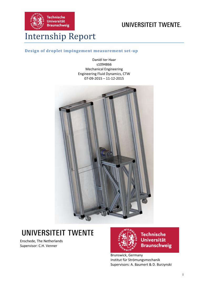
Internship Report

Design of droplet impingement measurement set-up

Daniël ter Haar s1094866

Mechanical Engineering Engineering Fluid Dynamics, CTW

07-09-2015 – 11-12-2015

Enschede, The Netherlands Supervisor: C.H. Venner

Brunswick, Germany Institut für Strömungsmechanik Supervisors: A. Baumert & D. Burzynski

ii

Preface From the beginning of September until halfway December I did my internship at the University of

Brunswick in Brunswick. I was stated at the Multiphase and Icing Flow research group located at the

Institute for Fluid Mechanics. In this time I helped several PhD students with their research.

Calibration of the icing wind tunnel, building and designing measurement set ups were few of the

many tasks. Since describing everything is unnecessary I chose to discuss the design of the new

droplet impingement wheel in this report in detail.

I would like to thank Arne Baumert and David Burzynski in particular for their guidance through this

internship. Arne for letting me help calibrate the multiphase wind tunnel and David for helping me

design parts of the droplet impingement wheel. I have learned in these few weeks a lot about how it

is to work at a research institute and which things I can expect when I would apply at a research

facility. I would like to ask David to send me a video of the system when it has actually been build. I

am very excited to see it in action and hear if everything works as it is supposed to.

iii

Summary This report covers the design of parts of the droplet impingement wheel. The goal is to design the

shaft, frame and safety screens and all the steps taken in this process are covered in this report.

Design criteria of the shaft, static strength analysis, dynamic strength analysis, final CAD design and

mounting order are presented.

Design criteria The flowing media should be methanol, ethanol and water in this watertight system. The wheel

should rotate at velocities between 250 rpm and 1000 rpm with a maximum deviation of ±0.01 at

1000 rpm. A confocal chromatic sensor should be used in combination with an optic rotary joint in

order to measure the film thickness during the rotation. Steady film requirement during the whole

rotation should be achieved by making sure that eigenfrequencies of the system are at least five

times higher than the actuating frequency.

Static strength analysis In the static strength analysis minimum shaft diameter as well as reaction forces on the bearings are

calculated. The shear force and moment are determined as function of the position in the parts are

presented and used to calculate the maximum shear force and maximum internal moment. Also the

endurance life of the bearings is estimated.

Dynamic strength analysis The eigenfrequencies of the shaft and medium and optical signal supply system are estimated using

the theory of the dynamics of continuous systems. Bending, torsional and longitudinal vibration

eigenfrequencies are estimated for the shaft. For the medium and optical signal supply system only

bending vibrations can occur and eigenfrequencies for this case are estimated.

Final CAD design and mounting order The final design is presented with a rendered photograph and all the features covered discussed.

Mounting order of all the parts is shown with guiding pictures and comments.

Frame and safety screens The design of the complete frame including safety screens is presented with rendered pictures. Since

the frame is built out of standard components the components as well as their functionality is

explained.

iv

Table of Contents Preface ......................................................................................................................................................ii

Summary ................................................................................................................................................. iii

Actual experiment ................................................................................................................................... 1

Improving the design ............................................................................................................................... 2

Subsystems of the design ........................................................................................................................ 3

Designed parts ......................................................................................................................................... 5

Power system ...................................................................................................................................... 5

Medium and optical signal supply system .......................................................................................... 5

Supporting frame ................................................................................................................................ 6

Designing the power system and medium and optical signal supply system ......................................... 6

Design specifications ........................................................................................................................... 7

Static strength analysis ........................................................................................................................ 7

Dynamical strength analysis .............................................................................................................. 10

Power system keys analysis............................................................................................................... 14

Seal design ......................................................................................................................................... 14

CAD Designs ....................................................................................................................................... 16

Mounting order and rendered photo ................................................................................................ 17

Designing the frame .............................................................................................................................. 18

Frame ................................................................................................................................................. 18

Building blocks ................................................................................................................................... 18

Designing the safety screens ................................................................................................................. 20

Used screens...................................................................................................................................... 20

Glass thickness .................................................................................................................................. 20

Appendix A: Measurement equipment configuration ............................................................................. I

Appendix B: Results from static strength analysis .................................................................................. II

Appendix B: Results from static strength analysis (continued) .............................................................. III

Appendix C: Dynamic strength analysis results ...................................................................................... IV

Appendix D: Power system keys analysis results .................................................................................... V

Appendix E: O-ring and groove dimensions ........................................................................................... VI

1 | P a g e

Actual experiment Since David Burzynski has to continue the research done by its predecessor B.W. Faẞmann first the

abstract of part of his research will be given:

“The vertical impact of single, mono dispersed water droplets on a dry smooth surface was studied experimentally by means of shadowgraphy. A glass substrate was mounted on a rotating wheel to obtain high impact velocities. The droplets were generated on demand. While the Ohnesorge number was kept constant, Weber number and Reynolds number were varied by adjusting the impact velocity. In all performed experiments, splashing was observed. The distinction of the different measurement series was done by the use of the Weber number. The different Weber numbers were, 3,500, 5,000 and 10,000. Phase-locked images were taken and the temporal evolution of the impact was reconstructed by means of the nondimensional impingement time. The outcome of the measurement was analyzed by digital image processing to quantify the distribution of the diameter of the resulting secondary droplets in size and time as well as their velocity, and the total deposited mass fraction remaining on the surface after the impingement. In all cases, the greater part of the impinging primary droplet remained on the substrate.” 1

If one then would take a look at the set-up (Figure 1) one could see the functions this design had:

- To create the high velocity impact of the droplets the wheel was rotated at high rotational velocities.

- The droplet generator made the droplets and released them with a trigger. This meant that the diameter of the droplets could be chosen as well as the moment the droplet would hit the surface.

- The syringe pump transports the medium to the droplet generator and controls the droplet volume.

- The trigger light barrier sends a signal to the system and triggers the camera and light source making sure that every picture that is taken contains a droplet.

1 W.B. Faẞmann (2013) High velocity impingement of single droplets on a dry smooth surface Exp Fluids (2013)

54:1516

Figure 1: Experimental set-up by W.B. Faẞmann (2013)

2 | P a g e

Improving the design In order to improve and extend the research of Faẞmann David Burzynski has the following

requirements:

- The experiments should also be done on wet surfaces so a steady film should be introduced

on the rotating surface.

- The range of the Weber number should be increased. Since the Weber number is

proportional to the density the media used for the droplets should be varied between water

ethanol and methanol. These properties give the opportunity to change the Reynolds

number while keeping the Weber number constant. Also the Weber number is quadratically

proportional to the velocity so the maximum rotation velocity of the wheel should be

increased.

- The accuracy of the wheel’s rotation should be improved. Especially when the system runs at

low velocities the actual velocity of the wheel deviates too much from the set velocity. This

leads to difficulties in synchronizing the system.

- The impact angle should be varied. The previous experiments were all done with a 90 degree

angle between the surface and droplet. Change in this angle could be very interesting and

should be examined.

- An optic sensor should be used in combination with an optic rotary joint to measure the film

thickness during the whole rotation of the system.

- It should be possible to implement a heating element in the future at the position of the film.

Heating the film could be interesting as an extension of the research. In order to be able to

implement this heating system power should be supplied to the rotating surface. This means

that either the optic rotary joint should also include a power connection or two separate slip

rings should be implemented.

- Because of the high rotational velocities of the wheel in the future a breaking system and

also a safety screen frame should be added to the system. If there are some problems with

the measurement or the system David wants to be able to break the system in order to make

it as safe as possible. Also the breaking system should possibly be triggered with an external

acceleration sensor on the wheel. This means that if some vibrations occur that are not

visible the system should detect these and break the wheel. The safety screens make sure

that if for instance the rotating surface releases nobody gets injured. Medium that drips

down the surface can be collected at the bottom and reused.

Since these are the new requirements the measurement system should have it is also very important

to learn from the first experiments made by Faẞmann. Since he was the first one to address the

problem several problems occurred during the experiments which should be solved in the new

design. Faẞmann tried to introduce the water film but has not succeeded because he was not able to

create a steady film at high velocities. The problems that need to be solved are:

- Close attention should be payed to making the system watertight. Because of the many leaks

the system had the created water film was never steady. Since this is the requirement to

publish the results all the measurements were not published.

- All the vibrations in the rotating system should be as low as possible. Due to these vibrations

the water film was disturbed with waves.

3 | P a g e

Subsystems of the design In order to efficiently develop the new design the choice was made to divide the whole design into

subsystems. Every subsystem had its specifications and problems and was solved separately. If one

would look at the complete design the following parts could be recognized (see Figure 2):

- The rotating surface (“Paddle”): This surface would convert the medium supply into a steady

film and has a collection device to suck away the medium and air mixture. Also the optical

sensor is used to measure the film thickness during the rotation of the Paddle.

- Rotating wheel: Should rotate at a fixed velocity without vibrations in any way so that the

film of the Paddle is uniform and the experiments can be made as consistently as possible to

make the experiments reproducible. One way to do this there should be a system included in

the wheel that enables the change of the moment of inertia. Also there should be a

possibility to connect the necessary tubings that provides the Paddle with medium and

extracts the medium and air mixture. The system trigger is on a fixed position on the wheel

making sure that every component needed for a good picture is activated at the right time.

- Medium and optic signal supply system: Inserts the medium and extracts the medium and air

mixture. The optical cable should enter the system here since at the motor no room is

available due to the direct contact between the shaft and the motor. Since this is the

connection of the static part to the rotating part a rotational joint must be implemented. The

optical cable is connected to a control box.

- Power system: Is the connection of the rotating shaft of the wheel to the motor, the breaking

system and the motor itself. This system is connected to the supporting frame and controlled

with the measurement equipment.

- Medium pump and mixture suction pump: inserts the medium into the system and extracts

the medium and air mixture.

- Supporting Frame: All the important parts are connected to a very sturdy frame. This to make

sure that there are as few vibrations as possible. Once the set-up is mounted all the distances

to all the components are fixed and aligned.

- Droplet generator: contains the droplet trigger as well as the syringe pump. This system

makes sure that all the droplets that hit the Paddle are as uniform as possible and hit the

Paddle at the moment when the photo is taken.

- Measurement equipment: Contains all the equipment that is needed to make the pictures at

the right moment and as consistent as possible. These components contain the camera(s),

laser, computer, Programmable Timing Unit (PTU), sensor control box and all the

connections between these components. The measurement set-up of the old experiment can

be found in Appendix A.

4 | P a g e

Figure 2: Complete design divided into subsystems

5 | P a g e

Designed parts In this chapter I would like to discuss the

parts of the design that I designed. The

total design consists also out of parts that

I consulted in but not designed myself

and thus will not be presented here. The

parts that I actually designed myself are

the power system, medium and optical

signal supply system, the supporting

frame and the safety screens. Since the

designs were supposed to be

improvements of the old design I first

discuss the old designed parts and state

the problems with these components.

When all the improvements that are

needed are known a model is made of the future design and several calculations are made to proof

that the future design will not fail during its use.

Power system Looking at the old power system (Figure 3) one can see that the wrong bearings are chosen. Simple

ball bearings constrain axial movement and since this is done twice the system is overdetermined.

Extra care needs to be taken into choosing the right bearings for the future design. Mounting the

tubes to the shaft was very difficult due to the limited space and needs to be made easier in the new

design.

Medium and optical signal supply

system Even though the old design (Figure 4) did

not contain the optical signal support taking

a close look at the old medium supply

system was very useful to exactly find where

the problems were and how they could be

solved.

The first problem is that the flows are not

separated at the location highlighted in

green. This means that the inflow to the

Paddle can also contain air which disturbs

the steady flow. Secondly the seals highlighted in light blue were not properly designed and caused

leakage. Third problem was the choice of bearings. The bearing that is shown in red is a simple ball

bearing that constrains axial displacement and in combination with the two ball bearings on the

power system meant that the system was overdetermined. This caused unnecessary stresses on the

bearings. Final and most important problem was the poor combination of materials. Some steel

parts were connected to aluminum parts and caused corrosion.

Figure 3: Schematic representation of the old power system. Bearings (red) ,supporting frame (gray), mix of in- and outflow (green) and closing rings (blue).

Figure 4: Schematic representation of old water supply system. inflow (dark blue), mix of in- and outflow (green) and outflow (yellow)

6 | P a g e

Supporting frame As can be seen in (Figure 5) the old supporting

frame consists out of two equal parts that are

connected with the floor connection flanges. Due to

the welded connections the tolerances of the frame

were too high making the connections to the floor

very difficult. Also the space between the bars was

too small causing mounting difficulties. Mounting

the motor was done externally using X-95 profiles

and created alignment issues. The overall problem

was that the old frame took too much space

compared to the functions it had. The new frame

should be smaller and have more functions besides

holding the wheel.

Designing the power system and medium and optical signal supply

system At the shaft medium supply, optical signal supply and also the rotational velocity of the wheel are

achieved. Since there are two positions on the shaft where these features can be inserted a

combination of two components was needed. The choice to combine the medium and optical signal

at one side and the power supply on the other side was made. Due to the rigid connection of the

shaft and engine there was not enough space to fit in another feature. The other option was to use a

belt between the shaft and the engine but this could introduce alignment problems and thus

unnecessary vibrations. Since I was responsible for the design of these components I would like to

describe here in detail the steps I took to make the original ideas into the final design. Since this

process can be described in chronological order I present these as the following phases:

- As in every design I started listing the design specifications that we made.

- Static strength analysis and dynamical strength analysis: A full static strength analysis is

made and determines the reaction forces and important stresses so that the right bearings

can be chosen as well as the right geometry. Also a dynamical strength analysis is done to

estimate the eigenfrequencies of the two systems. This chapter gives only the derivation of

the formulas and the formulas itself. For the static strength analysis results see Appendix B

and for the dynamical strength analysis results see Appendix C.

- Power system keys analysis: The torque of the motor needs to be converted into rotational

velocity of the wheel. The connection of the motor to the shaft and wheel is by the usage of

keys. In order to make sure that the keys are strong enough the maximum stress as function

of the applied torque needs to be determined. This chapter gives only the derivation of the

formulas and the formulas itself. For the power system keys analysis results see Appendix D.

- Seal design: Making the system watertight had proven to be difficult in the past so extra time

and effort was spent on the design of the O-rings and also choosing the right material for this

Figure 5: Schematic representation of the old frame. Frame (gray) and connection to the ground (red)

7 | P a g e

application. This chapter gives only the derivation of the formulas and the formulas itself. For

the O-ring and groove dimensions see Appendix E.

- CAD Design: Since at this stage all the requirements of the system are known the design is

made and presented.

- Mounting order and rendered photo: Special care was taken to make the system simple to

mount and the way to do is explained here. In the last step the complete system is visualized

with a rendered photograph.

Design specifications In order to make sure that all the requirements can be achieved and checked at the end of the design

some quantifiable numbers need to be addressed to the system requirements (Table 1):

System requirement Specified range

Rotational velocity of the wheel 250 rpm – 1000 rpm

Maximum deviation of the rotational velocity ±0.01 rpm at 1000 rpm

Media useable in system Water, ethanol and methanol

Optic sensor to measure the film thickness during the whole rotation of the wheel

Confocal Chromatic Sensor

Optic rotary joint + electrical slip ring Single channel-multimode optic fiber

Breaking system (should be triggered by accelerator sensor on the wheel)

Implemented in electric motor or separate system

System watertight No leakage of medium anywhere

No disturbing vibrations Eigen frequencies of rotating system 5 times higher than actuating frequency (>100 Hz)

Film quality Steady film over the whole rotation with uniform thickness and no disturbance waves.

Table 1: Design specifications

Static strength analysis

Reaction forces and maximum

stresses on the power system

The bearings that support the shaft are

chosen such that the system is simply

supported and thus statically determined.

This means that there is one bearing that

can be represented by a roll support and

one bearing that can be represented by a

normal not moving support. If one then

would take a look at the Free Body

Diagram (see Figure 6) the reaction forces

on the bearings can be easily calculated and are:

∑𝐹𝑥 = 0 ⇒ 𝐹𝑥1 = 0

∑𝐹𝑦 = 0 𝑎𝑛𝑑 ∑𝑀𝑧 = 0 ⇒

Figure 6: Free Body Diagram shaft

8 | P a g e

𝐹𝐴 = 𝐹𝑙𝑜𝑎𝑑 ∗ (𝐿1−𝑥1

𝐿1) , 𝐹𝐵 = 𝐹𝑙𝑜𝑎𝑑 ∗

𝑥1

𝐿1 𝒘𝒊𝒕𝒉

𝒙𝟏

𝑳𝟏>

𝟏

𝟐

Now the forces on the bearings are known thus an estimate can be made of the lifespan of the

bearings2:

𝐿10 = (𝐶

𝐹)𝑝

, {𝐶: 𝑑𝑦𝑛𝑎𝑚𝑖𝑐 𝑙𝑜𝑎𝑑 𝑓𝑎𝑐𝑡𝑜𝑟 [𝑁]𝐹: 𝑓𝑜𝑟𝑐𝑒 𝑜𝑛 𝑏𝑒𝑎𝑟𝑖𝑛𝑔 [𝑁]

𝑝: 𝑙𝑖𝑣𝑒𝑙𝑖𝑓𝑒 𝑒𝑥𝑝𝑜𝑛𝑒𝑛𝑡 [−]

𝐿10: 𝐿𝑖𝑓𝑒 𝑒𝑥𝑝𝑒𝑐𝑡𝑎𝑛𝑐𝑦 [𝑛𝑜. 𝑟𝑜𝑡𝑎𝑡𝑖𝑜𝑛𝑠]

The internal shear force and internal moment as function of the position are:

𝑉1(𝑥) = {𝐹𝐴

𝐹𝐴 − 𝐹𝑙𝑜𝑎𝑑𝑓𝑜𝑟

0 ≤ 𝑥 < 𝑥1𝑥1 < 𝑥 ≤ 𝐿1

𝑎𝑛𝑑 𝑀1(𝑥) = {𝐹𝐴𝑥

𝐹𝐴𝑥 − 𝐹𝑙𝑜𝑎𝑑(𝑥 − 𝑥1) 𝑓𝑜𝑟

0 ≤ 𝑥 < 𝑥1𝑥1 < 𝑥 ≤ 𝐿1

The maximum internal shear stress of the shaft and also the maximum bending stress can then be

determined:

𝜏𝑠ℎ𝑒𝑎𝑟,𝑚𝑎𝑥 =𝑉1,𝑚𝑎𝑥

𝐴𝑠𝑜𝑙𝑖𝑑 𝑠ℎ𝑎𝑓𝑡=|𝐹𝐴 − 𝐹𝑙𝑜𝑎𝑑|

𝜋𝑟𝑠ℎ𝑎𝑓𝑡2, 𝜎𝑏𝑒𝑛𝑑𝑖𝑛𝑔,𝑚𝑎𝑥 =

𝑀1(𝑥1) ∗ 𝑟𝑠ℎ𝑎𝑓𝑡

𝐼𝑠𝑜𝑙𝑖𝑑 𝑠ℎ𝑎𝑓𝑡=𝐹𝐴 ∗ 𝑥1 ∗ 𝑟𝑠ℎ𝑎𝑓𝑡𝜋4 𝑟𝑠ℎ𝑎𝑓𝑡

4

Now these two formulas can be used to calculate the minimum solid shaft diameter for the shear

stress and bending stress. The larger of the two is the minimum solid shaft diameter that is needed

so that the shaft will not fail due to static forces.

𝑑𝑚𝑖𝑛,𝑠ℎ𝑒𝑎𝑟 = 2√|𝐹𝐴−𝐹𝑙𝑜𝑎𝑑|

𝜋∗𝜏𝑚𝑎𝑥

𝑑𝑚𝑖𝑛,𝑏𝑒𝑛𝑑𝑖𝑛𝑔 = 2 ∗ √4∗𝐹𝐴∗𝑥1

𝜋∗𝜎𝑚𝑎𝑥

3

Reaction forces and maximum stresses

on the medium and optical signal

supply system

The same procedure can be done to

calculate the important values for the water

and optical signal system (for Free Body

Diagram see Figure 7):

∑𝐹𝑥 = 0 ⇒ 𝐹𝑥2 = 0

∑𝐹𝑦 = 0 𝑎𝑛𝑑 ∑𝑀𝑧 = 0 ⇒

𝐹𝐶 = 𝐹𝐴 ∗ (𝐿2−𝑥2

𝐿2) , 𝐹𝐷 = 𝐹𝐴 ∗

𝑥2

𝐿2, 𝒘𝒊𝒕𝒉

𝒙𝟐

𝑳𝟐<

𝟏

𝟐

2 Catalogue Schaeffler KG, (2008) “Wälzlager”

Figure 7: Free Body Diagram water and optical signal system

9 | P a g e

Now the forces on the bearings are known thus an estimate can be made of the lifespan of the

bearings3:

𝐿10 = (𝐶

𝐹)𝑝

, {𝐶: 𝑑𝑦𝑛𝑎𝑚𝑖𝑐 𝑙𝑜𝑎𝑑 𝑓𝑎𝑐𝑡𝑜𝑟 [𝑁]𝐹: 𝑓𝑜𝑟𝑐𝑒 𝑜𝑛 𝑏𝑒𝑎𝑟𝑖𝑛𝑔 [𝑁]

𝑝: 𝑙𝑖𝑣𝑒𝑙𝑖𝑓𝑒 𝑒𝑥𝑝𝑜𝑛𝑒𝑛𝑡 [−]

𝐿10: 𝐿𝑖𝑓𝑒 𝑒𝑥𝑝𝑒𝑐𝑡𝑎𝑛𝑐𝑦 [𝑛𝑜. 𝑟𝑜𝑡𝑎𝑡𝑖𝑜𝑛𝑠]

The internal shear force and internal moment as function of the position are:

𝑉2(𝑥) = {𝐹𝐶

𝐹𝐶 − 𝐹𝐴𝑓𝑜𝑟

0 ≤ 𝑥 < 𝑥2𝑥2 < 𝑥 ≤ 𝐿2

𝑎𝑛𝑑 𝑀2(𝑥) = {𝐹𝐶𝑥

𝐹𝐶𝑥 − 𝐹𝐴(𝑥 − 𝑥2) 𝑓𝑜𝑟

0 ≤ 𝑥 ≤ 𝑥2𝑥2 < 𝑥 ≤ 𝐿2

The maximum internal shear stress of the medium system and also the maximum bending stress can

then be determined:

𝜏𝑠ℎ𝑒𝑎𝑟,𝑚𝑎𝑥 =𝑉2,𝑚𝑎𝑥

𝐴𝑠𝑜𝑙𝑖𝑑 𝑠ℎ𝑎𝑓𝑡=

𝐹𝐶𝜋𝑟𝑠ℎ𝑎𝑓𝑡

2, 𝜎𝑏𝑒𝑛𝑑𝑖𝑛𝑔,𝑚𝑎𝑥 =

𝑀2(𝑥2) ∗ 𝑟𝑠ℎ𝑎𝑓𝑡

𝐼𝑠𝑜𝑙𝑖𝑑 𝑠ℎ𝑎𝑓𝑡=𝐹𝐶 ∗ 𝑥2 ∗ 𝑟𝑠ℎ𝑎𝑓𝑡𝜋4𝑟𝑠ℎ𝑎𝑓𝑡

4

Now these two formulas can be used to calculate the minimum solid shaft diameter for the shear

stress and bending stress. The larger of the two is the minimum solid shaft diameter that is needed

so that the shaft will not fail due to static forces.

𝑑𝑚𝑖𝑛,𝑠ℎ𝑒𝑎𝑟 = 2𝑟𝑚𝑖𝑛,𝑠ℎ𝑒𝑎𝑟 = 2√𝐹𝐶

𝜋∗𝜏𝑚𝑎𝑥, 𝑑𝑚𝑖𝑛,𝑏𝑒𝑛𝑑𝑖𝑛𝑔 = 2𝑟𝑚𝑖𝑛,𝑏𝑒𝑛𝑑𝑖𝑛𝑔 = 2 ∗ √

4∗𝐹𝐶∗𝑥2

𝜋∗𝜎𝑚𝑎𝑥

3

3 Catalogue Schaeffler KG, (2008) “Wälzlager”

10 | P a g e

Dynamical strength

analysis

Eigenfrequencies of the

power system

In order to calculate the

estimated eigenfrequencies of

the power system one has to

look first at the theory of the

dynamics of continuous systems.

In this case three load cases can

be found and also vibrations in

these directions are very

important. In order to be able to

calculate analytic solutions to

these equations a simplified

model of the system is

introduced (see Figure 8). The

mass and inertia are introduced

as representation of the wheel and due to this

discontinuity the domain needs to be split into two pieces. Also the distinction is made between the

different load cases. As one can see the boundary conditions slightly differ for the different

configurations.

Bending vibrations

The equation of motion that needs to be solved for bending vibrations of continuous systems

(homogenous and prismatic shaft):

𝜌𝐴𝜕2𝑣(𝑥,𝑡)

𝜕𝑡2+ 𝐸𝐼

𝜕4𝑣(𝑥,𝑡)

𝜕𝑥4= 𝐹(𝑥, 𝑡)

In order to calculate the eigenfrequencies of the unforced system the solution is found by the

separation of variables method (only for standing waves):

𝑣(𝑥, 𝑡) = 𝑋(𝑥)𝑇(𝑡), ⇒𝑇′′

𝑇= −

𝐸𝐼

𝜌𝐴∗𝑋′′′′

𝑋= −𝜔2

So the equations that need to be solved are:

𝑇′′(𝑡) + 𝜔2𝑇(𝑡) = 0, 𝑋′′′′(𝑥) − 𝛽4𝑋(𝑥) = 0, 𝛽4 =𝜌𝐴

𝐸𝐼𝜔2

And the solutions to these differential equations are:

𝑇(𝑡) = 𝐴𝑡𝑐𝑜𝑠(𝜔𝑡) + 𝐵𝑡𝑠𝑖𝑛(𝜔𝑡)

𝑋(𝑥) = 𝐴𝑥 cos(𝛽𝑥) + 𝐵𝑥 sin(𝛽𝑥) + 𝐶𝑥 cosh(𝛽𝑥) + 𝐷𝑥sinh (𝛽𝑥)

Figure 8: Vibrational model for the power system

11 | P a g e

Now the general solution of the differential equation is known. In order to make the solution realistic

for the chosen model the constants and frequencies need to be determined. Due to the

concentrated mass one equation to describe the whole system is not enough. In this case two

functions are used that are valid in the two parts of the domain.

𝑣1(𝑥1, 𝑡) = 𝑋1(𝑥1)𝑇1(𝑡) 𝑓𝑜𝑟 0 ≤ 𝑥1 ≤ 𝑎 𝑣2(𝑥2, 𝑡) = 𝑋2(𝑥2)𝑇2(𝑡) 𝑓𝑜𝑟 0 ≤ 𝑥2 ≤ 𝐿 − 𝑎

The easy boundary conditions that come with this configuration are:

𝑣1(0, 𝑡) = 0, 𝐸𝐼𝜕2𝑣1

𝜕𝑥12 |𝑥1=0

= 0, ⇒ 𝐴𝑥1 = 𝐶𝑥1 = 0

𝑣2(𝐿 − 𝑎, 𝑡) = 0, 𝐸𝐼 𝜕2𝑣2

𝜕𝑥22 |𝑥2=𝐿−𝑎

= 0

𝜕𝑣1

𝜕𝑥1|𝑥1=𝑎

= 𝜕𝑣2

𝜕𝑥2|𝑥2=0

, 𝑣1(𝑎) = 𝑣2(0)

At the position of the mass the equations need to be connected to satisfy continuity conditions and

also the acceleration of the mass needs to be accounted for. To determine odd and even functions

the boundary conditions slightly differ:

∑𝐹𝑦 = 𝐹2 ∓ 𝐹1 = 𝑚0𝑎0 = 𝑚0𝑣1̈ ⇒ 𝐸𝐼 (𝜕3𝑣2

𝜕𝑥23 |𝑥2=0

∓𝜕3𝑣1

𝜕𝑥13 |𝑥1=𝑎

) =𝑚0𝜕

2𝑣2

𝜕𝑡2|𝑥2=0

∑𝑀 = 𝑀2 ∓𝑀1 = 𝐽0𝛼 ⇒ 𝐸𝐼 (𝜕2𝑣2

𝜕𝑥22 |𝑥2=0

∓ 𝜕2𝑣1

𝜕𝑥12 |𝑥1=𝑎

) = 𝐽0𝜕3𝑣2

𝜕𝑥𝜕𝑡2|𝑥2=0

Where the minus sign determine the odd functions and the plus sign the even functions. All these

conditions can be written in matrix vector form. Since this multiplication is equal to zero the trivial

solution can be found which means a static system or if the determinant is zero the eigenfrequencies

are found (b=L-a).

[

0 00 0

𝑐𝑜𝑠 (𝛽𝑏) 𝑠𝑖𝑛 (𝛽𝑏)

−𝛽2𝑐𝑜𝑠 (𝛽𝑏) −𝛽2𝑠𝑖𝑛 (𝛽𝑏)

𝑐𝑜𝑠ℎ (𝛽𝑏) 𝑠𝑖𝑛ℎ (𝛽𝑏)

𝛽2𝑐𝑜𝑠ℎ (𝛽𝑏) 𝛽2𝑠𝑖𝑛ℎ (𝛽𝑏)

𝛽𝑐𝑜𝑠 (𝛽𝑎) 𝛽𝑐𝑜𝑠ℎ (𝛽𝑎)𝑠𝑖𝑛 (𝛽𝑎) 𝑠𝑖𝑛ℎ (𝛽𝑎)

0 −𝛽1 0

0 −𝛽1 0

𝛽3𝑐𝑜𝑠 (𝛽𝑎) −𝛽3𝑐𝑜𝑠ℎ (𝛽𝑎)

𝛽2𝑠𝑖𝑛(𝛽𝑎) −𝛽2𝑠𝑖𝑛ℎ (𝛽𝑎)

𝑚0𝜔2

𝐸𝐼∓𝛽3

∓𝛽2𝐽0𝜔

2

𝐸𝐼𝛽

𝑚0𝜔2

𝐸𝐼±𝛽3

±𝛽2𝐽0𝜔

2

𝐸𝐼𝛽 ]

{

𝐵𝑥1𝐷𝑥1𝐴𝑥2𝐵𝑥2𝐶𝑥2𝐷𝑥2}

=

{

000000}

So now the eigenfrequencies of the system can be calculated simply by substituting all values for the

system and finding for which 𝜔 the determinant of the matrix is equal to zero. To check if the

solution is valid one can check a special case which is known. Since for a simply supported beam

without mass the eigenfrequencies are known:

𝜔𝑛 = 𝑛2𝜋2√

𝐸𝐼

𝜌𝐴𝐿4 𝑓𝑜𝑟 𝑛 = 1,2,…∞

This is validated and the eigenfrequencies of the system are equal to the theoretical values.

12 | P a g e

Torsional vibrations

The equation of motion that needs to be solved for torsional vibrations of continuous systems

(homogenous and prismatic shaft):

𝜌𝐽𝜕2Θ(𝑥,𝑡)

𝜕𝑡2− 𝐺𝐽

𝜕2Θ(𝑥,𝑡)

𝜕𝑥2= 𝑇(𝑥, 𝑡)

The same process as shown in bending vibrations can be used to determine the solutions to the

unforced equation:

𝑇(𝑡) = 𝐴𝑡𝑐𝑜𝑠(𝜔𝑡) + 𝐵𝑡𝑠𝑖𝑛(𝜔𝑡)

𝑋(𝑥) = 𝐴𝑥 cos(𝛽𝑥) + 𝐵𝑥 sin(𝛽𝑥)

𝑤𝑖𝑡ℎ 𝛽2 =𝜌

𝐺𝜔2

The simple boundary conditions for the clamped-free shaft and the connection of the functions:

Θ1(𝑥1 = 0) = 0, 𝐺𝐽𝜕Θ2

𝜕𝑥2|𝑥2=𝐿−𝑎

= 0, Θ1(𝑥1 = 𝑎) = Θ2(𝑥2 = 0)

Due to the concentrated mass in the middle and thus polar moment of inertia (note that due to the

unsymmetrical boundary conditions even functions are not possible):

𝐺𝐽 (𝜕Θ2

𝜕𝑥2|𝑥2=0

−𝜕Θ1

𝜕𝑥1|𝑥1=𝑎

) = 𝐼0𝜕2Θ2

𝜕𝑡2|𝑥2=0

= −𝜔2𝐼0Θ2(𝑥2 = 0)

The system of equations that needs to be solved is (b=L-a):

[

1 00 0

0 0−𝛽𝑠𝑖𝑛 (𝛽𝑏) 𝛽𝑐𝑜𝑠 (𝛽𝑏)

𝑐𝑜𝑠 (𝛽𝑎) 𝑠𝑖𝑛 (𝛽𝑎)𝛽𝑠𝑖𝑛 (𝛽𝑎) −𝛽𝑐𝑜𝑠 (𝛽𝑎)

−1 0𝜔2𝐼0

𝐺𝐽𝛽 ]

{

𝐴𝑥1𝐵𝑥1𝐴𝑥2𝐵𝑥2

} = {

0000

}

If one then would check the special case when the polar moment is equal to zero and a=L/2 one can

validate the model to the theoretical eigenvalues the system should have:

𝜔𝑛 =𝑛𝜋

2𝐿√𝐺

𝜌, 𝑓𝑜𝑟 𝑛 = 1,3,5,… ,∞

This is validated and the eigenfrequencies of the system are equal to the theoretical values.

Longitudinal vibrations

The equation of motion that needs to be solved for longitudinal vibrations of continuous systems

(homogenous and prismatic shaft):

𝜌𝐴𝜕2𝑢(𝑥,𝑡)

𝜕𝑡2− 𝐸𝐴

𝜕2𝑢(𝑥,𝑡)

𝜕𝑥2= 𝑁(𝑥, 𝑡)

The same process as shown in bending vibrations can be used to determine the solutions to the

unforced equation:

13 | P a g e

𝑇(𝑡) = 𝐴𝑡𝑐𝑜𝑠(𝜔𝑡) + 𝐵𝑡𝑠𝑖𝑛(𝜔𝑡), 𝑋(𝑥) = 𝐴𝑥 cos(𝛽𝑥) + 𝐵𝑥 sin(𝛽𝑥) , 𝛽2 =

𝜌

𝐸𝜔2

The simple boundary conditions are:

𝑢1(𝑥1 = 0) = 0,𝜕𝑢2

𝜕𝑥2|𝑥2=𝐿−𝑎

= 0, 𝑢1(𝑥1 = 𝑎) = 𝑢2(𝑥2 = 0)

Force equilibrium at the concentrated mass gives:

𝐸𝐴(𝜕𝑢2

𝜕𝑥2|𝑥2=0

−𝜕𝑢1

𝜕𝑥1|𝑥1=𝑎

) = 𝑚0𝜕2𝑢2

𝜕𝑡2|𝑥2=0

The matrix vector equation will then be:

[

1 00 0

0 0−𝛽𝑠𝑖𝑛 (𝛽𝑏) 𝛽𝑐𝑜𝑠 (𝛽𝑏)

𝑐𝑜𝑠 (𝛽𝑎) 𝑠𝑖𝑛 (𝛽𝑎)𝛽𝑠𝑖𝑛 (𝛽𝑎) −𝛽𝑐𝑜𝑠 (𝛽𝑎)

−1 0𝜔2𝑚0

𝐸𝐴𝛽 ]

{

𝐴𝑥1𝐵𝑥1𝐴𝑥2𝐵𝑥2

} = {

0000

}

If one then would check the special case when the polar moment is equal to zero and a=L/2 one can

validate the model to the theoretical eigenvalues the system should have:

𝜔𝑛 =(2𝑛−1)𝜋

2𝐿∗ √

𝐸

𝜌 𝑓𝑜𝑟 𝑛 = 1,2,3,… ,∞

This is validated and the eigenfrequencies of the system are equal to the theoretical values.

Eigenfrequencies of the water and optical signal supply system

For the water and optical signal supply system only bending vibrations are important since torsion

and longitudinal directions are not exited.

The theory of solving the equations is equal

as presented for the power system only the

boundary conditions are different.

The boundary conditions that come with this

configuration are:

𝑣(0, 𝑡) = 0,𝜕𝑣

𝜕𝑥|𝑥=0

= 0

𝑣(𝐿, 𝑡) = 0, 𝐸𝐼 𝜕2𝑣

𝜕𝑥2|𝑥=𝐿

= 0

The system of equations that needs to be solved is:

[

1 00 𝛽

1 00 𝛽

𝑐𝑜𝑠 (𝛽𝐿) 𝑠𝑖𝑛 (𝛽𝐿)

−𝛽2𝑐𝑜𝑠 (𝛽𝐿) −𝛽2𝑠𝑖𝑛(𝛽𝐿)

𝑐𝑜𝑠ℎ (𝛽𝐿) 𝑠𝑖𝑛ℎ (𝛽𝐿)

𝛽2𝑐𝑜𝑠ℎ (𝛽𝐿) 𝛽2𝑠𝑖𝑛ℎ (𝛽𝐿)

] {

𝐴𝑥𝐵𝑥𝐶𝑥𝐷𝑥

} = {

0000

} 𝑤𝑖𝑡ℎ 𝛽4 =𝜌𝐴

𝐸𝐼𝜔2

And the eigenfrequencies are found when the determinant is equal to zero.

Figure 9: Vibrational model medium and optical signal supply system

14 | P a g e

Power system keys analysis In order to guide the power delivered by the motor

to the shaft and onto the wheel keys are used. Since

these keys should sustain shear stress and

compression stress to guide the torsional moment

formulas for these are derived (for free body diagram

see Figure 10):

𝑇 = 𝐹 ∗𝐷

2⇒ 𝜏𝑠ℎ𝑒𝑎𝑟 =

𝐹

𝐴𝑠ℎ𝑒𝑎𝑟 𝑝𝑙𝑎𝑛𝑒=

2𝑇

𝐷𝑊𝐿

𝜎𝑐𝑜𝑚𝑝𝑟𝑒𝑠𝑠𝑖𝑜𝑛 =𝐹

0.5∗𝐴𝑐𝑜𝑚𝑝𝑟𝑒𝑠𝑠𝑖𝑜𝑛 𝑝𝑙𝑎𝑛𝑒=

4𝑇

𝐷𝐻𝐿

Since the two load cases appear at the same time the

maximum stresses that appear in the key are the

principal stresses according to:

𝜎1 =𝜎𝑐𝑜𝑚𝑝𝑟𝑒𝑠𝑠𝑖𝑜𝑛

2+√(

𝜎𝑐𝑜𝑚𝑝𝑟𝑒𝑠𝑠𝑖𝑜𝑛

2)2+ 𝜏𝑠ℎ𝑒𝑎𝑟

2 , 𝜎2 =𝜎𝑐𝑜𝑚𝑝𝑟𝑒𝑠𝑠𝑖𝑜𝑛

2−√(

𝜎𝑐𝑜𝑚𝑝𝑟𝑒𝑠𝑠𝑖𝑜𝑛

2)2+ 𝜏𝑠ℎ𝑒𝑎𝑟

2

To ensure that the key not fails during use the maximum principal stress should not exceed the

maximum allowed stress of the key. For a simple case the maximum allowed stress can be the yield

stress of the material but in order to account for fatigue and other failure mechanisms it is common

to use a safety factor. This means that the maximum allowed stress of the key is the yield stress

multiplied with a safety factor.

𝑖𝑓 {𝜎1 ≥ 𝜎2 𝜎2 ≥ 𝜎1

𝑡ℎ𝑒𝑛 {𝜎1 ≤ 𝜎𝑚𝑎𝑥𝜎2 ≤ 𝜎𝑚𝑎𝑥

, 𝑤ℎ𝑒𝑟𝑒 𝜎𝑚𝑎𝑥 = 𝑁𝑠𝑎𝑓𝑒𝑡𝑦 ∗ 𝜎𝑦𝑖𝑒𝑙𝑑 𝑤ℎ𝑒𝑟𝑒 [1 ≤ 𝑁𝑠𝑎𝑓𝑒𝑡𝑦 ≤ 4]

Seal design

Dimensions

To ensure a watertight system as well as

to make sure that the in- and outflow

cannot mix O-rings need to be designed.

To fix the O-ring in the groove the initial

O-ring diameter should be smaller than

the groove diameter so that the O-ring is

slightly stretched and snugly fitting.

𝑂𝐷 =𝐺𝐷

1+%𝑠𝑡𝑟𝑒𝑡𝑐ℎ 𝑤ℎ𝑒𝑟𝑒 1 ≤ %𝑠𝑡𝑟𝑒𝑡𝑐ℎ ≤ 5

The cross section diameter of the O-ring

should be such that for every possible

tolerance combination the hole is

completely closed. Since the system is

rotating a percentage of compression is

Figure 10: Free body diagram of keys

Figure 11: O-ring sketch

15 | P a g e

introduced to make sure that the O-ring is exerting force onto the surface and seals perfectly:

The maximum cross section diameter of the O-ring is:

𝑚𝑎𝑥(𝑅𝑖𝑛𝑔𝐶.𝑆.𝐷) =(𝑚𝑖𝑛𝐵𝑜𝑟𝑒𝐷−𝑚𝑎𝑥𝐺𝑟𝑜𝑜𝑣𝑒𝐷

2)

1−𝑚𝑎𝑥(%𝑐𝑜𝑚𝑝𝑟𝑒𝑠𝑠𝑖𝑜𝑛)− 𝑅𝑖𝑛𝑔𝐶.𝑆.𝐷 𝑡𝑜𝑙𝑒𝑟𝑎𝑛𝑐𝑒 , 𝐶. 𝑆. 𝐷. = 𝐶𝑟𝑜𝑠𝑠 𝑆𝑒𝑐𝑡𝑖𝑜𝑛 𝐷𝑖𝑎𝑚𝑒𝑡𝑒𝑟

In the same way the minimum cross section diameter can be determined:

𝑚𝑖𝑛(𝑅𝑖𝑛𝑔𝐶.𝑆.𝐷)) =(𝑚𝑎𝑥𝐵𝑜𝑟𝑒𝐷−𝑚𝑖𝑛𝐺𝑟𝑜𝑜𝑣𝑒𝐷

2)

1−𝑚𝑖𝑛(%𝑐𝑜𝑚𝑝𝑟𝑒𝑠𝑠𝑖𝑜𝑛)+ 𝑅𝑖𝑛𝑔𝐶.𝑆.𝐷 𝑡𝑜𝑙𝑒𝑟𝑎𝑛𝑐𝑒

Due to the rotational velocity the percentage of compression influences the amount of friction

generated by the O-rings. For dynamical purposes a compression percentage between 10% and 30%

is commonly used.

Used material

Since the O-ring should endure water, ethanol and methanol not all materials can be used. Also low

friction should be introduced so a hard material should be selected. Combining these requirements

with the fact that the medium is used at room temperature gives the best material for this purpose

to be ethylene propylene diene terpolymer (commonly called EPDM).

Surface roughness

To reduce friction and wear the rotating surface should be as smooth as possible. Also the groove

should have some surface roughness to keep the O-ring from rotating. The recommended4 surfaces

roughness’s are:

For {𝐶𝑜𝑛𝑡𝑎𝑐𝑡 𝑠𝑢𝑟𝑓𝑎𝑐𝑒:

𝐺𝑟𝑜𝑜𝑣𝑒:

𝑅𝑚𝑒𝑎𝑛 = 1.6𝜇𝑚𝑅𝑚𝑒𝑎𝑛 = 3.2 𝜇𝑚

and 𝑅𝑚𝑎𝑥 = 6.3𝜇𝑚𝑅𝑚𝑎𝑥 = 12.5𝜇𝑚

and should be implemented.

4 https://www.parker.com/literature/ORD%205700%20Parker_O-Ring_Handbook.pdf

16 | P a g e

CAD Designs

Here the final CAD-designs (see Figure 12) of the power, medium and optical signal supply systems

are presented. The subsystems that can be recognized are:

- In- and outflow: From the static part on the left the medium flows through the top channel

to the rotating chamber. This chamber is always filled with medium and secured from

leakage with O-rings. From the rotating chamber it flows through the shaft and into a tube

that is connected to the paddle. On the way back it enters another rotating chamber which is

secured with O-rings and leaves the static part on the lower channel.

- Bearings: The shaft is simply supported using one simple ball bearing (on the right) and one

needle bearing without inner ring (on the left). The simple ball bearing constrains movement

in x- and y-direction whereas the needle bearing enables x-direction movement. The medium

and optical signal supply system has two needle cage bearings and these are used to direct

the forces from the shaft to the frame and relieve possible forces on the O-rings. X-direction

movement is enabled and is used to insert the system into the shaft.

- Closing rings: All the closing rings are used to make sure that after mounting the bearings

and wheel are only able to move in the directions they are supposed to. On the other side of

the bearings solid edges are used to center the bearings.

- Hybrid slip contact: The hybrid slip contact consists out of two slip rings that are combined

to one product. The optical signal slip ring is placed inside an electrical slip contact and fixed

there. The total product can be bought and is fixed on the static part using M4 screws. The

optical cable leaves the slip contact and is directed to the wheel at a big radius to prevent

signal loss.

- Housings: The bearing housings are used to fix the whole shaft system to the frame. On the

left there can be seen that the medium and optical supply system is fixed to the housing

using M8 screws.

- Keys: As mentioned in “Power system keys analysis” keys are used to guide the torque of the

motor to the wheel.

Figure 12: CAD designs of the power, medium and optical signal supply systems

17 | P a g e

Mounting order and rendered photo The right way to mount the whole shaft system is

presented here. Several subsystem mounting orders

are explained and the rendered photograph of the

total system will be given.

1. Medium and optical signal supply system

Every part that should be fixed on the system should

be inserted from the right and slide into negative x-

direction (see Figure 13). First the bigger needle cage

should be pressed onto the solid surface and secured

with the closing ring. Then the six O-rings can be fixed

in their grooves. After the O-rings the second needle

cage plus closing ring can be fixed. Last step is securing

the hybrid slip contact with four M4 screws making

sure that the cables are fitted through the gaps.

2. Fixed bearing and wheel

First the simple ball bearing should be fixed on the

shaft and secured with its closing ring. Second the

bearing should be fixed in the casing and closed with

its corresponding closing ring. Final step is sliding the

wheel on the shaft from the left (see Figure 14) and

fixed by its closing ring and key.

3. Floating bearing

Fixing the needle bearing (see Figure 15) in its casing is

the same process as done with the simple ball bearing.

After the bearing is fixed the shaft can be mounted in

the bearing. NOTE: no closing ring necessary here due

to axial freedom of the shaft at this position.

4. Securing the medium and optical signal

supply system (rendered photograph)

The final step for the whole assembly is sliding the

whole medium and optical signal supply system in the

shaft and fixing it with three M8 screws. In Figure 16

the result of the last step can be seen. The whole

assembly including the wheel can now be mounted on

the frame.

Figure 13: Mounting medium and optical signal supply system

Figure 14: Mounting the simple ball bearing and wheel (wheel not displayed)

Figure 15: Mounting needle bearing in its casing and shaft in bearing

Figure 16: Rendered photo of cut of final assembly shaft system

18 | P a g e

Designing the frame In this chapter I would like to present the new

frame which I designed. After taking a close

look at the old frame the choice has been

made to make the frame out of standard

elements provided by a well-known company

in Germany5. The aluminum profiles that are

used can be easily connected to make a light

and stiff construction. Also the possibility to

change things in the future or adding new

features can be easily achieved. This was very

difficult with the old frame due to the welded

connections. All the connections in the new

frame will be made by using standard building

blocks which use M8 screws.

Frame As can be seen in Figure 17 the frame consists

out of standard aluminum profiles which are

connected in a way to create trusses. The two

parts that can be recognized are the motor

support and the medium supply support which

are connected with four profiles. On the right the part that supports the motor can be seen. The

plate on which the motor is mounted is connected to the frame and separated with rubber foam to

reduce vibrations. The two bearing cases

are also protected from vibrations using

rubber foam.

Building blocks

Profiles

The profiles6 that are used have a particular

shape (see Figure 19). Indicated in grey is

the actual geometry whereas the other

colors are to indicate other functions. The

blue parts are cavities where the so called

“Nutenstein7” can fit (see Figure 18). These

are parts that can slide over the whole length of the profile and can be used to fix other parts to

these profiles. The big hole in the middle which is indicated in green can be used once there is a

threading tapped in there to connect parts on the ends of the profiles. The orange cavities are weight

reductions.

5 http://www.item24.de/produkte/item-baukastensysteme/mbsystembaukasten.html

6 http://product.item24.de/produkte/produktkatalog/products/profile-und-zubehoer-1.html

7 http://product.item24.de/produkte/produktkatalog/products/nutensteine.html

Figure 17: Rendered photo of frame

Figure 19: Cross section of aluminum profile “Profil 8 40x40 leicht natur”

Figure 18: "Nutenstein" and screw

19 | P a g e

Corner connections

In the design four types of corner

connections are used. These are:

Verbindungssatz 8 40x40x40 8

This connection can be used once

in the middle of the profile a

threading is tapped and connects

up to three profiles. In the design

these connectors are used to

create the cube that supports the

motor and create the frame for the

medium support. In Figure 17 these

connections can be seen as black

cubes.

Winkelelement 8 T1-40 9

This connector block is used to fix a

45 degree angled profile in a corner

(see Figure 21). The T1 connector as

well as the T2 connector are used

for creating the trusses and can be found in Figure 17 as black triangles.

Winkelelement 8 T2-40 10

This connector block is used to fix two 45 degree angled profiles to each other and to a 90 degree

profile as can be seen in Figure 22. The T2 connector as well as the T1 connector are used for

creating the trusses and can be found in Figure 17 as black triangles.

Gehrungs-Verbindungssatz 8 11

The last connector (see Figure 23) is used for fixing parts that are at strange angles. Since the frames

are not twice as high as wide the angle of the profile is not 45 degrees and another connector is

needed. In Figure 17 these connectors are not explicitly drawn since they are fixed inside the profiles.

Six of these are used to connect the three angled profiles.

8 http://product.item24.de/produkte/produktkatalog/produktdetails/products/eck-

verbindungssaetze/verbindungssatz-8-40x40x40-schwarz-41608.html 9

http://product.item24.de/produkte/produktkatalog/produktdetails/products/winkelelemente/winkelelement-8-t1-40-natur-38800.html 10

http://product.item24.de/produkte/produktkatalog/produktdetails/products/winkelelemente/winkelelement-8-t2-40-natur-38802.html 11

http://product.item24.de/produkte/produktkatalog/produktdetails/products/gehrungs-verbindungssaetze/gehrungs-verbindungssatz-8-49230.html

Figure 20: "Verbindungssatz 8 40x40x40" Figure 21: "Winkelelement 8 T1-40"

Figure 22: "Winkelelement 8 T2-40" Figure 23: "Gehrungs-Verbindungssatz 8"

20 | P a g e

Designing the safety screens The safety screens that have been

designed are presented in Figure 24. Also

these screens are made out of the

standard profiles and assembled using M8

screws. Two parts can be distinguished

and are both supported by wheels to

make the system mobile. At the left the

more complex safety screen can be seen

which features a hole for the droplets (on

the top) and holes in the other parts for

cameras and lasers. Since the screens are

made out of safety glass images can be

distorted and holes are necessary. One

can see that at the very left the hole in the

screen is as small as possible. In order to

protect the camera from a possible

breaking paddle the slit is smaller than the

paddle.

Used screens Since the material of the screens endures

water, ethanol and methanol not all

materials will suffice. In fact all possible

clear plastics were not resistant to the

three combinations of materials. Since normal glass is resistant to all these media the choice has

been made to make the safety screens out of safety glass. Safety glass is stronger than normal glass

and can endure the high impact of the paddle. To make sure that the glass does not break at impact

the minimum thickness needs to be calculated.

Glass thickness The impact energy of the paddle needs to be calculated in order to choose the right glass thickness:

𝐸𝑖𝑚𝑝𝑎𝑐𝑡 =1

2𝑚𝑝𝑎𝑑𝑑𝑙𝑒 ∗ 𝑣𝑝𝑎𝑑𝑑𝑙𝑒

2 =1

2∗1

2∗ (30)2 = 225 𝐽𝑜𝑢𝑙𝑒𝑠

So with making the choice for the glass one must take care that the glass can endure 225 Joules. The

glass that is chosen12 has a thickness of 6 mm thick and meets the specifications necessary.

12

http://www.glas-behrens.de/catalog/sicherheitsglaeser/7ab17f67-a039-4dad-9ca9-49f8dfddf64c.aspx

Figure 24: Rendered photograph of safety screens

I | P a g e

Appendix A: Measurement equipment configuration

II | P a g e

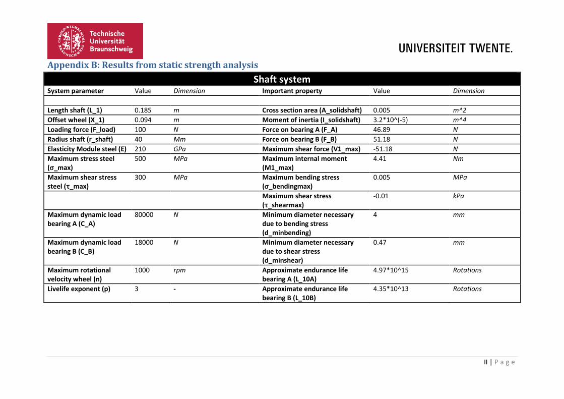
Appendix B: Results from static strength analysis

Shaft system System parameter Value Dimension Important property Value Dimension

Length shaft (L_1) 0.185 m Cross section area (A_solidshaft) 0.005 m^2

Offset wheel (X_1) 0.094 m Moment of inertia (I_solidshaft) 3.2*10^(-5) m^4

Loading force (F_load) 100 N Force on bearing A (F_A) 46.89 N

Radius shaft (r_shaft) 40 Mm Force on bearing B (F_B) 51.18 N

Elasticity Module steel (E) 210 GPa Maximum shear force (V1_max) -51.18 N

Maximum stress steel (σ_max)

500 MPa Maximum internal moment (M1_max)

4.41 Nm

Maximum shear stress steel (τ_max)

300 MPa Maximum bending stress (σ_bendingmax)

0.005 MPa

Maximum shear stress (τ_shearmax)

-0.01 kPa

Maximum dynamic load bearing A (C_A)

80000 N Minimum diameter necessary due to bending stress (d_minbending)

4 mm

Maximum dynamic load bearing B (C_B)

18000 N Minimum diameter necessary due to shear stress (d_minshear)

0.47 mm

Maximum rotational velocity wheel (n)

1000 rpm Approximate endurance life bearing A (L_10A)

4.97*10^15 Rotations

Livelife exponent (p) 3 - Approximate endurance life bearing B (L_10B)

4.35*10^13 Rotations

III | P a g e

Appendix B: Results from static strength analysis (continued)

Medium and optical signal supply system System parameter Value Dimension Important property Value Dimension

Length shaft (L_2) 0.087 m Cross section area (A_solidshaft) 0.002 m^2

Offset wheel (X_2) 0.0073 m Moment of inertia (I_solidshaft) 3.2*10^(-6) m^4

Loading force (F_A) 46.89 N Force on bearing C (F_C) 42.98 N

Radius shaft (r_shaft) 22.5 Mm Force on bearing D (F_D) 3.9 N

Elasticity Module steel (E)

210 GPa Maximum shear force (V2_max) 42.98 N

Maximum stress steel (σ_max)

500 MPa Maximum internal moment (M2_max)

0.312 Nm

Maximum shear stress steel (τ_max)

300 MPa Maximum bending stress (σ_bendingmax)

0.002 MPa

Maximum shear stress (τ_shearmax)

27.02 kPa

Maximum dynamic load bearing C (C_C)

29500 N Minimum diameter necessary due to bending stress (d_minbending)

2 mm

Maximum dynamic load bearing D (C_D)

22500 N Minimum diameter necessary due to shear stress (d_minshear)

0.43 mm

Maximum rotational velocity wheel (n)

1000 rpm Approximate endurance life bearing C (L_10C)

3.23*10^14 Rotations

Livelife exponent (p) 3 - Approximate endurance life bearing D (L_10D)

1.92*10^17 Rotations

IV | P a g e

Appendix C: Dynamic strength analysis results

Shaft system System parameter Value Dimension Important property Value Dimension

Length shaft (L_1) 0.185 m Cross section area (A_hollowshaft) 0.0017 m^2

Offset wheel (X_1) 0.094 m Moment of inertia (I_hollowshaft) 1.82*10^(-5) m^4

Mass wheel (m_0) 10 kg

Polar moment of inertia wheel for bending (J_0) 0.42 kg*m^2 First bending eigenfrequency 6333 Rad/s

Polar moment of inertia wheel for torsion (I_0) 0.84 kg*m^2 Second bending eigenfrequency 26250 Rad/s

Outer radius shaft (r_out) 40 mm

Inner radius shaft (r_in) 32.5 mm First torsional eigenfrequency 6013 Rad/s

Elasticity Module steel (E) 210 GPa Second torsional eigenfrequency 54300 Rad/s

Shear Module steel (G) 79.3 GPa

Density steel (𝛒) 7700 kg/m^3 First longitudinal eigenfrequency 18370 Rad/s

Maximum rotational velocity 1000 Rpm Second longitudinal eigenfrequency 91430 Rad/s

Maximum rotational velocity 104.7 Rad/s

Medium and optical signal supply system System parameter Value Dimension Important property Value Dimension

Length shaft (L_2) 0.125 m Cross section area (A_hollow) 0.0015 m^2

Outer radius shaft (r_out) 25 mm Moment of inertia (I_hollow) 4.60*10^(-6) m^4

Inner radius shaft (r_in) 12.5 mm

Elasticity Module steel (E) 210 GPa First bending eigenfrequency 288100 Rad/s

Density steel (𝛒) 7700 kg/m^3 Second bending eigenfrequency 933600 Rad/s

Maximum rotational velocity 1000 Rpm

Maximum rotational velocity 104.7 Rad/s

V | P a g e

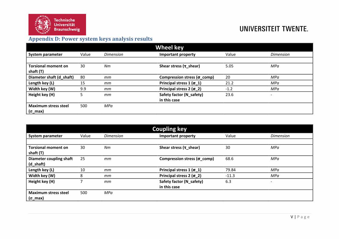
Appendix D: Power system keys analysis results

Wheel key System parameter Value Dimension Important property Value Dimension

Torsional moment on shaft (T)

30 Nm Shear stress (𝛕_shear) 5.05 MPa

Diameter shaft (d_shaft) 80 mm Compression stress (𝛔_comp) 20 MPa

Length key (L) 15 mm Principal stress 1 (𝛔_1) 21.2 MPa

Width key (W) 9.9 mm Principal stress 2 (𝛔_2) -1.2 MPa

Height key (H) 5 mm Safety factor (N_safety) in this case

23.6 -

Maximum stress steel (σ_max)

500 MPa

Coupling key System parameter Value Dimension Important property Value Dimension

Torsional moment on shaft (T)

30 Nm Shear stress (𝛕_shear) 30 MPa

Diameter coupling shaft (d_shaft)

25 mm Compression stress (𝛔_comp) 68.6 MPa

Length key (L) 10 mm Principal stress 1 (𝛔_1) 79.84 MPa

Width key (W) 8 mm Principal stress 2 (𝛔_2) -11.3 MPa

Height key (H) 7 mm Safety factor (N_safety) in this case

6.3 -

Maximum stress steel (σ_max)

500 MPa

VI | P a g e

Appendix E: O-ring and groove dimensions O-ring and Groove dimensions (see Figure 11)

Important property Value Dimension

O-ring diameter 56.88 mm

O-ring cross section diameter 1.78 mm

O-ring cross section diameter tolerances ±0.08 mm

O-ring material EPDM

Groove diameter 57.4 mm

Groove width 2.4 mm

Bore diameter 60 mm

Maximum diametrical clearance 0.068 mm

Minimum diametrical clearance 0.030 mm

Groove and surface material Stainless steel 1.4571

Mean contact surface roughness 1.6 𝜇m

Maximum contact surface roughness 6.3 𝜇m

Mean groove surface roughness 3.2 𝜇m

Maximum contact surface roughness 12.5 𝜇m