1

Internet Futures: Unlocking user bottlenecks

Barr, T., Knowles, A. & Moore, S.

Swinburne University of Technology, School of Social and Behavioural Sciences (Mail 24)

PO Box 218, Hawthorn, Vic Australia, 3122.

Email of presenter: smoore@swin.edu.au Abstract The notion of ‘bottlenecks’ for Internet users emerged as a useful umbrella concept to categorise a range of impediments to the uptake of Internet based transaction services in Australia. This paper reports the results of a study of barriers influencing Internet consumers, Internet providers views of what consumers want/need, and factors associated with potential up-take of new forms of mobile phone commercial transactions. The methodology was focus groups and in-depth interviews. Trust emerged as an important predictor of consumer behaviour, for both Internet and potential m-commerce users. The perception that users have of the (lack of) security of their transactions on the Internet is a major inhibiting factor to the growth of on-line services. While trust was also an issue for mobile phone users who might consider m-commerce, a mitigating factor against risk perception was the perception of the mobile phone as an extension of self (and therefore somehow more trustworthy). Interestingly, providers did not see the complex issues of trust in the same light as users. They drew a distinction between the consumer sense of trusting the Internet as a medium of communications as opposed to the ‘trusted’ brand reputation of the merchants. Implications for Internet futures are discussed. Introduction The primary focus of this research, entitled ‘Internet futures: Unlocking user bottlenecks’ was to understand how consumers and providers perceive the risks associated with Internet transactions, and what factors inhibit on- line consumers. There were three principal strands of research within this project, managed across three Australian Universities - Swinburne University, RMIT (Network Insight) and CTIN (Adelaide University). Each of these groups employed different but complementary methodologies. In the case of the work undertaken at Swinburne and Adelaide Universities focus groups were the prime methodology employed to elicit the views of users about their interaction with the Internet. Adelaide based research focused on user responses to possible new mobile commerce services. In the

case of RMIT (Network Insight) the investigation was conducted from the viewpoint of some of the providers (strategists) through in-depth interviews. This paper integrates the findings of these three segments. In summary, this research project examined the complex social and behavioural issues relating to the way Australian men and women interact with the Internet in transactional contexts. The investigation was conducted from both the viewpoint of end users and the providers of transactional services. Background literature

Past research on the uptake of e-commerce is mostly US based and concerns Internet shopping, rather than encompassing the broader range of Internet transactions such as share purchasing, banking and negotiating home loans. Nevertheless the role of trust has been identified in many of these earlier studies.

Jarvenpaa, Tractinsky and Saarinen (1999) showed that across three different countries, perceived merchant reputation and to a lesser extent perceived merchant size were important predictors of consumer trust, while more general personal factors like shopping enjoyment, attitudes toward computers and web-shopping risk beliefs (for example about security) had little effect on intentions to buy on the Internet. Swaminathan, Lepkowska-White and Roa (1999) found personal characteristics of the shopper more influential than consumer confidence or trust in the medium. In their American study using a non-random e-mail survey to approximately 400 participants, they found that convenience as a shopping motive was a more important predictor of on-line shopping than vendor characteristics, although vendor reputation, and perceived security, were also predictors. Using an on-line survey of US Internet users, Hairong, Kuo and Russell (1999) tested the role of a comprehensive range of factors in predicting on-line buying. Significant predictors were distribution utility, accessibility, channel knowledge, experiential orientation, convenience

2

orientation, and higher levels of education. These factors together accounted for 27% of the variance in Internet users’ on-line buying behaviour. Smith and Swinyard (2001) analysed the factors which online shopping households disliked about Internet shopping by distributing 4,000 questionnaires to on line shoppers in 50 US states. They concluded that key factors were shipping charges, reluctance to use credit cards on the Internet, problems with the quality of the merchandise and difficulties associated with returning merchandise. The four survey studies reported above showed somewhat different patterns of results, with Jarvenpaa et al. emphasising merchant trust, Swaminathan et al. emphasising consumer characteristics, Hairong et al. emphasising channel knowledge, or web experience, and Smith and Swinyaard emphasising the fears of Internet shoppers as the most important factors predicting on-line buying. The variables used the studies were overlapping but different, as were analyses used, so the studies are not directly comparable. The most significant Australian work in this area began with Singh’s Connecting Customers and Providers: A focus on Electronic Money (1997). This concluded that ‘recognition of trust as an important factor of use came only during a late stage of analysis… trust had not been central to the questions asked in the interviews…once the question was redefined, it became clear there was a big hole in the collection and initial analysis of data…. The issues of trust lay wholly in the background.’ (Singh, 1997: 10) Subsequent related work, based on a qualitative study of 47 people, came to the principal conclusion that ‘people are more likely to use a form of payment they trust.’ (Singh & Slegers 1997: 3) This work also drew upon US research in suggesting that ‘hard trust' deals with issues of authenticity, encryption and security of transactions and ‘soft trust’ clusters around control, comfort and caring. We need to re-think this framework since it implies that the complex issues concerning consumers’ sense of trust in Internet trading may be easier to resolve than the technology security issues. For the purpose of this study we explored, within an Australian context, the perceived reliability and integrity of the Internet as a communications medium by consumers in the context of commercial transactions. We focussed on trust, or lack of perceived trust, as an overarching ‘bottleneck’ in Internet transactions but we also explored a range of other possible barriers to commercial Internet transactions from several perspectives. While there has been much written about m-commerce, the literature summary report done for Telstra (Arnold and Associates 2001) showed there is very little about users and

prospective users related to m-commerce, so this aspect of Internet transactions was a special focus of one segment of the study.

Methodology Each segment of this project established

its own methodologies, as described below. Victorian research (Swinburne)

This section of the study was conducted by Barr, Knowles and Moore. A qualitative methodology was adopted, designed to increase understanding of the bottlenecks/barriers to Internet transactions and to explore the cognitive, emotional and behavioural consumer processes that surround them. The project was based around targeted focus groups with Internet users and non-users of both genders, from a range of age, geographic and socio-economic groups. A threshold qualification for inclusion was that people used the Internet; people who did not use the Internet were excluded. Those who used it less than once a week were rated low channel knowledge; those who used it for e-mail and occasionally for other purposes up to three times a week were rated medium channel knowledge, and those who used it for e-mail and other purposes on most days were rated high channel knowledge. Five focus groups each made up of eight respondents were interviewed in Melbourne (4) and Warrnambool (1) in March 2002. The groups recruited contained males and females, with no more than five of one gender in a group of eight. There were three groups of medium channel knowledge participants (two ‘white-collar’, one ‘blue collar’), one in which channel knowledge was low and one in which it was high. Two of the groups represented the ‘under 30s’ age group, two were 30-54, and one group was 55 years and above. Thus groups reflected different levels of channel knowledge, gender, age, education/socio-economic status and the rural/urban variable. Questions were asked about reasons they used the Internet, major usage areas, experiences (both good and bad), of buying goods and services on the Internet, concerns and issues about credit card usage, experiences using the Internet for banking, buying shares or negotiating home loans, beliefs about the security and convenience of the Internet, relative importance of trust in comparison with other potential barriers/facilitators in Internet transactions, and how the Internet could work better. Discussions were audio-taped. New South Wales research (RMIT)

This segment of the project (conducted by Armstrong) examined the views of on-line merchants and service providers about bottlenecks which can affect consumer use of the Internet. The

3

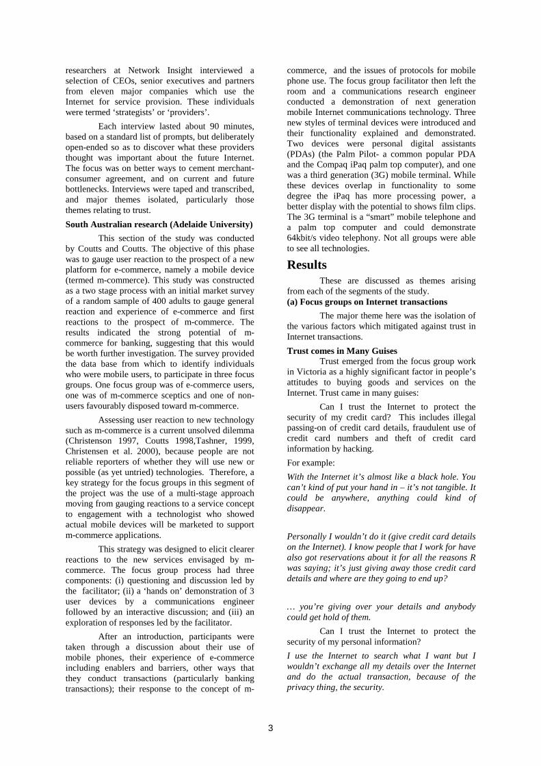
researchers at Network Insight interviewed a selection of CEOs, senior executives and partners from eleven major companies which use the Internet for service provision. These individuals were termed ‘strategists’ or ‘providers’. Each interview lasted about 90 minutes, based on a standard list of prompts, but deliberately open-ended so as to discover what these providers thought was important about the future Internet. The focus was on better ways to cement merchant-consumer agreement, and on current and future bottlenecks. Interviews were taped and transcribed, and major themes isolated, particularly those themes relating to trust. South Australian research (Adelaide University)

This section of the study was conducted by Coutts and Coutts. The objective of this phase was to gauge user reaction to the prospect of a new platform for e-commerce, namely a mobile device (termed m-commerce). This study was constructed as a two stage process with an initial market survey of a random sample of 400 adults to gauge general reaction and experience of e-commerce and first reactions to the prospect of m-commerce. The results indicated the strong potential of m-commerce for banking, suggesting that this would be worth further investigation. The survey provided the data base from which to identify individuals who were mobile users, to participate in three focus groups. One focus group was of e-commerce users, one was of m-commerce sceptics and one of non-users favourably disposed toward m-commerce. Assessing user reaction to new technology such as m-commerce is a current unsolved dilemma (Christenson 1997, Coutts 1998,Tashner, 1999, Christensen et al. 2000), because people are not reliable reporters of whether they will use new or possible (as yet untried) technologies. Therefore, a key strategy for the focus groups in this segment of the project was the use of a multi-stage approach moving from gauging reactions to a service concept to engagement with a technologist who showed actual mobile devices will be marketed to support m-commerce applications. This strategy was designed to elicit clearer reactions to the new services envisaged by m-commerce. The focus group process had three components: (i) questioning and discussion led by the facilitator; (ii) a ‘hands on’ demonstration of 3 user devices by a communications engineer followed by an interactive discussion; and (iii) an exploration of responses led by the facilitator. After an introduction, participants were taken through a discussion about their use of mobile phones, their experience of e-commerce including enablers and barriers, other ways that they conduct transactions (particularly banking transactions); their response to the concept of m-

commerce, and the issues of protocols for mobile phone use. The focus group facilitator then left the room and a communications research engineer conducted a demonstration of next generation mobile Internet communications technology. Three new styles of terminal devices were introduced and their functionality explained and demonstrated. Two devices were personal digital assistants (PDAs) (the Palm Pilot- a common popular PDA and the Compaq iPaq palm top computer), and one was a third generation (3G) mobile terminal. While these devices overlap in functionality to some degree the iPaq has more processing power, a better display with the potential to shows film clips. The 3G terminal is a “smart” mobile telephone and a palm top computer and could demonstrate 64kbit/s video telephony. Not all groups were able to see all technologies.

Results These are discussed as themes arising

from each of the segments of the study. (a) Focus groups on Internet transactions

The major theme here was the isolation of the various factors which mitigated against trust in Internet transactions. Trust comes in Many Guises

Trust emerged from the focus group work in Victoria as a highly significant factor in people’s attitudes to buying goods and services on the Internet. Trust came in many guises:

Can I trust the Internet to protect the security of my credit card? This includes illegal passing-on of credit card details, fraudulent use of credit card numbers and theft of credit card information by hacking. For example: With the Internet it’s almost like a black hole. You can’t kind of put your hand in – it’s not tangible. It could be anywhere, anything could kind of disappear. Personally I wouldn’t do it (give credit card details on the Internet). I know people that I work for have also got reservations about it for all the reasons R was saying; it’s just giving away those credit card details and where are they going to end up? … you’re giving over your details and anybody could get hold of them.

Can I trust the Internet to protect the security of my personal information? I use the Internet to search what I want but I wouldn’t exchange all my details over the Internet and do the actual transaction, because of the privacy thing, the security.

4

…you hear stories of people obtaining credit card numbers and buying other goods, and you get lumped with the bill.

Can I trust this merchant to deal fairly and reliably with me? Will he deliver the merchandise I have paid for and will it be in good condition? …you can’t see the product before you get it.

Who can I hold accountable? Yeah if it turns up damaged, what course do you take?

What about after-sales service? If you buy something over the Internet and the goods come but they’re not the quality they should be: what happens then?

How do I know this is not a fly-by-night operator? …it would depend on who it was. If it was someone who you knew you could trust like a major big organisation you’re going to, someone like Telstra, as opposed to a name that you’ve never heard of which could be, you know, some little garage in Thailand somewhere. If we’re going to purchase over the Internet, go for a well-known company because you trust that a company that’s large has adequate protection for what we’re doing. They know the risks and they know what the obligations they are under and they can’t really afford not to have what they need.

These concerns were compounded by widespread lack of knowledge about who is ultimately liable if a transaction goes wrong: is it the consumer, the merchant, the bank? This pilot study essentially unravelled a range of factors about consumers’ perceived lack of trust, but did not attempt to quantify the variables. In summary the main factors were fears of credit card fraud, hackers, and invasion of privacy (worries about security), concerns about the merchant's reliability, delivery of goods, after sales service and accountability if things went wrong. To a large extent, 'trust' was seen as a problem with the Internet as a vehicle for transactions, rather than conceptualised as a problem of merchant reputation (although this was referred to by some users). Channel knowledge and Internet banking

The focus groups indicated that people appear reluctant to go into Internet banking without first thoroughly educating themselves in the procedures and the safeguards, and they put this off as likely to be time-consuming. Trust in the security of the Internet against credit card fraud and unauthorised disclosure of personal information appeared to be less of an issue in relation to Internet banking than other commercial

transactions because most people seem to believe that banks are good at security. There appeared to be a connection between level of channel knowledge and sense of consumer confidence with Internet banking: the more people were generally used to the Internet, the more likely they were to use it for banking purposes. (b) Interviews with strategists

The major themes here were that trust is built on brands/merchant reputation; on-line transactions are based on user-merchant relationships; the transaction interface must be simple. Trust built on reputation

Providers offered a different perspective to that which emerged about trust in the user focus groups. For them, the user’s trust and confidence came from outside the on-line experience. Their perspective was that even if users do not have positive feelings about a particular corporation, at least they think it has a reputation to maintain; so if something goes wrong the perception is that the corporation will fix the problem. While this idea was reflected to some extent in users' comments, it was viewed as highly important by providers, more so than concerns about credit card security, privacy, hackers and the like. Strategists also discussed forms of third party reassurance for consumers - the logos and certifications of bodies such as VeriSign and TRUSTe. Potentially, they can assure consumers that they are dealing with a site which will protect their data, or adhere to a particular privacy regime. The strategists did not consider that the logos or certification of these systems had much value for building consumer trust, despite their potential as the Internet develops. This negative view about consumer reassurance was despite the actual functionality of VeriSign-type systems, which encrypt data to and from the consumer so that PINs, personal data etc cannot be intercepted. Consciously or not, the strategists argue that users base their strategies on predicting the behaviour of the merchant (what it has to lose), rather than on technology. They also argued that consumers rarely understand or even read these certifications. Strategists acknowledged that people had been frightened about using cards online, but thought that the tide was turning. Nearly all believed that Australian consumers were readily entering card details on-line and that ‘market research does not seem to reflect the reality of consumer behaviour’. They argued that 'users appear less conservative in practice than what they tell market researchers'. Strategists were not sure how to account for the difference. One reported on his on-line ticketing experience in the US:

5

Call centres set up to take credit card details to close a transaction simply do not get the traffic. It seems to me that users, once they have committed think: ‘yes I do really want that airline ticket and to get it I have to enter my credit card, so, OK I will’

Another said: Clients tell me that customer resistance to giving credit card details has decreased significantly over the past two years and they put that down to a better understanding of the protection that use of a credit card affords them through the credit company terms. I think a lot of consumers are aware now that if you use a credit card on the Internet you effectively have the credit company standing behind you. A 2000-2001 ACNielsen Australia survey of 1.5 million users across 12 Asia-Pacific countries, including Australia, found this also (Lugo, 2002). Financial security, or concerns about the safety of using credit cards online, dropped to sixth in the list of concerns about Internet use, down from third just a year earlier. Fears of viruses, the cost of access, slow response times and spam were all rated as more serious. On-line transactions are based on relationships

These were the strategists’ three most-used images of a how Internet transactions happen: (i) An online conversation with the user, with some exchange of information (ii) A sequence of permission-giving by the user, who provides more input as the merchant makes it clear why the user should move on to the next step (iii) A quid pro quo deal, in which the user is offered an incentive to take up merchant offers.

Behind each of these images is respect for the intelligence or ‘savvy’ of the user. None of the strategists suggested that users will just grab an offer because it is there, or because it looks attractive. There was a widespread view that the merchant has to justify to the user why he or she should click further into the site, or sign up, or provide more information. Even where the transaction is a small one, such as subscribing to an information service or agreeing to receive e-mails, it is rarely a single moment. Nearly all the strategists said that an effective site is designed around an interactive process, so that the user will take the next step, which might be only providing an e-mail address, postcode or telephone number, or disclosing the user’s income bracket. Users baulk as soon as they feel confronted by requests for personal information or commitment before some kind of relationship is built, based on familiarity, comfort or trust. The challenge for the merchant is increased because users are also intolerant of time-wasting. The relationship-building might take less than a minute,

but it still has the same character. Strategists pointed out that consumers are intelligent, both about how much time they invest in a site, and also in deciding about the value proposition. The more useful or sought-after the product, the less likely it is that users will lie or withhold their personal information. For example: How much they tell you depends on what you are giving them in return. If it is something they value they’ll hand over their details and they will make sure they’re accurate. With subscriptions – where people genuinely want the product arriving on their doorsteps – we have about 99-100 percent accuracy. So it’s not really about tricking them, it’s about giving them something in return. Strategists pointed out that in on-line transactions, 'consumers hold the cards'. That is one reason why ‘trust’ is so fragile on line. Somehow, the merchant must have a way to maintain trust from second to second, for fear that the consumer will disappear. That is why so many of the strategists had been refining their sites, to ensure that the consumer could see a reason for taking the next step towards completion. The slightest distraction or frustration can be terminal. …the more information they ask you for, the greater the chance that you will drop out. Simplicity of the interface

The need for simplicity was one of the dominant themes to come out of the interviews. Strategists recalled the glamorous and glossy pages with multiple links offered during the dotcom boom as expensive, slow and ineffective, with between a five and 10 per cent success rate at converting visits into transactions or information aggregation. Most agreed that if a site is not simple in layout it will perform badly as a business tool: The rule of thumb is that people don’t read on the Internet, they skim. Everything needs to be reasonably blocky and if you can’t get the message out in 200 words, don’t bother.

Strategists said that it is difficult to project from the current Web experience to the future, because most users are still learning to use the Internet. Some made the point that the Internet as a retail channel is only about three years old, and should be seen as in its experimental stage. Some had noticed that users had learned more about how to transact on the Internet in the last two years. For example, travellers had come to understand what sort of tickets they were buying, whereas initially they had been more confused. There was some speculation that users would become slightly better at reading the text on a site or device. But this did not detract from the overwhelming commercial experience that simplicity is still the key. (c) Focus groups discussing m-commerce

6

Mobile – the personal friend Mobile users constitute a larger

percentage of the Australian population than computer/ e-commerce users. It may be more realistic to postulate the migration of new m-commerce applications from present mobile telephony than the more often assumed evolution of m-commerce applications from the e-commerce market. It appears more likely that mobile users who are not currently e-commerce users see the transition to m-commerce as natural or inevitable, especially when presented with attractive new m-commerce applications. Mobile phone users become attached to their phones in ways that are not reflected by the comments of computer users. For example: I would prefer to use that (new mobile device) than a computer at home because it is like a little friend

The mobile phone (and the future m-commerce platform) was viewed by users in a very personal sense as an extension of themselves enabling them to control their communications in a unique way. This very personal relationship with a communications device which in a sense “augments” the person is unique. It impacts on how users adopt and use mobile services in a way which is distinctive from the computer or TV. This aspect of the perception of a mobile phone as an extension of the person has been a subject of social science research but has never been captured in any research into adoption and practice of such devices.

However, although the mobile devices were popular among the focus groups, and they expressed fewer barriers toward using them for transactions than the focus groups discussing computer-based Internet transactions, the strategists were somewhat sceptical about these devices as a platform for transactions. You have to ask, ‘Is the [mobile] telephone a serious business thing or is it this fun lifestyle device?’ My kids use it for SMS but is it really something you use to transact? The usability world is still struggling about how I can get an 800x600 right, with the right information in there, with the right level of detail; so the entertainment stuff might happen within the next decade but for the transaction stuff, I don’t think so.

Conclusions e-commerce has many advantages for both

the consumer and the merchant, but barriers to trust in this medium for transacting are many and complex. The perceptions of different groups, reflected through the qualitative methodologies of focus groups and in-depth interviews, help to shed light on the various dimensions of these complexities and how they differ according to the

groups targeted and the particular type of Internet transaction being discussed. Large scale surveys are now needed to explore the relative importance of the different kinds of barriers and the extent to which they play a causal role in limiting Internet transactions.

References Arnold and Associates (2001). Review of literature related to the uptake of mobile telecommunication services and a conceptual framework for future research. Research report for Telstra.

Christensen, & Clayton (1997). The Innovators Dilemma: When new technologies cause great firms to fail, HBS Press: Massachusetts

Christensen et al (2000). Meeting the challenge of disruptive change, in Christensen, C.M., & Overdorf, M. Harvard Business Review 78, 66-76.

Coutts (1998). A user methodology – Identifying telecommunications needs in, Coutts, P.J. Communications Research Forum (CRF), Canberra, September 24-25, 1998. Hairong, L., Kuo, C., & Russell, M. (1999). The impact of perceived channel utilities, shopping orientations, and demographics on the consumers’ on-line buying behavior. Journal of Computer-Mediated Communication, 5(2). www.usc.edu/dept/annenberg. Jarvenpaa, S. L., Tractinsky, N., & Saarinen, L. (1999). Consumer trust in an Internet store: A cross-cultural validation. Journal of Computer-Mediated Communication, 5(2). www.usc.edu/dept/annenberg.

Lugo, L. M. T. (2002). Local retailers can still tap wide opportunities in online shopping. BusinessWorld, May 7, p.19 Singh, S. (1997) Connecting customers and providers: A focus on electronic money. Policy Research Paper no. 16, CIRCIT, Melbourne.

Singh, S., & Slegers, C. (1997) Trust and electronic money. Policy Research Paper no. 42, CIRCIT, Melbourne.

Smith, S., & Swinyard, W. (2001). The Internet Usability Study. Marriot School of Management, Brigham Young University.

Swaminathan, V., Lepkowska-White, E., & Rao, B.P. (1999). Browsers or buyers in cyberspace? An investigation of factors influencing electronic exchange. Journal of Computer-Mediated Communication, 5(2). www.usc.edu/dept/annenberg.

Tashner, R. (1999) Forecasting new telecommunication services at a “pre-development” product stage, in Loomis, D.G., & Taylor, L.D. (1999). The Future of the Telecommunications Industry: Forecasting and Demand Analysis.

Acknowledgements: This paper reports on research conducted by T. Barr, M. Armstrong, P. Coutts, R. Coutts, A. Knowles, & S. Moore.

!!#"%$'&!(*)$'',+-$/.0'(1243*567$89

:<;>=@?BADCFEGIHKJL=MAKNADCMOBPQRATS@;IUTNVXWYNZHZ[>\K]^O>P`_a?#YZ\'bUdce\K]f;Igh]f[Vi

Ojlkmnko(prqsqtvuvw^oxzywnpruxDuM|uM~pDqsxzywnprukkxDo>|uvBywnytMykz uvwrkBwypD~lprmnm^pruMrpruvvd rrr@MtMByxDm^w^x

qsxDwnmflqsk(vxDuywnytvpZk(vtxDtv-@p@o>wetvpZk(vtxDti pDypDprm^xtv¡yxzm^w¢xkBk£xDBo>9¤¥k(uykz¦ §¨prBXy£R©¥pDyxDuTrR@ rDrdvªtvByxDmnw¢x` q xzw^mf B@RL«tMyw^k(wno¬£q'pDyprprm^xMoprq

­¯®-°@±³²¯­´a±µ¶·¹¸MºK»#ºD¼¡½ºK½¾¼¸¿¼BÀ(Á¸v»lÀ¼Bà ÄÅLÆIÇK»IÅZÈvÆ(¸¾·Áf·Æ(À·ÀKÉÊ£ËZ¸¿ÌÁf¼¡Í<Î^Ä`ÈÏÊÐeÌ^Çz»I¸¾¼Bѽ¾Æ(ÒZÁ¾·LÀɨº½fÆ#ÁfÆZÓÔÆIÅ^ÕBÓB»#ÅLżÑ`ÖÆZÓ¡»#Á¾·LÆIÀZÌÇK»(¸¿¼ÑFÈvÆ(·ÀÁ¿Ì^Á¾ÆIÌ^ºDÆI·LÀÁ×ØÑ»#ºZÁf·Ù(¼Ú¨ÆIÒZÁf·ÀKÉXÎnÖ@ÈT×lÚØÐÛ Æ(½ÜÍÆIÇ·LÅL¼Ø»IѶÆZÓÝÀ¼¡ÁÃÏÆ(½¾ÞZ¸BßMµ¶·¹¸Ïº½¾ÆIÁ¾ÆZÓÔÆ(ÅKÒZÁf·ÅL·¹¸¿¼¸»à>Ìe¸¿Áf»>Áf¼ª½fÆIÒÁ¾¼ÑZ·¹¸¾Ó¡Æ>ÙI¼B½¾Ë¸¿Á¾½Â»>Á¾¼BÉIË·LÀ»ºzÆ(·ÀÁ¿Ì^Á¾ÆI̺DÆI·LÀÁÍ-»IÀÀ¼¡½ÁfÆ ½f¼BÑÒKÓÔ¼½¾Æ(ÒZÁ¾·LÀÉ Æ>ÙI¼B½¾¶¼»IÑè¶K·ÅL¼Í-»>áZ·LÍ·L¸¾·ÀKÉÁf¶½¾Æ(ÒÉI¶KºÒZÁ-·ÀͼBÑ·ÒÍâÁ¾ÆŹ»#½fÉI¼¯ÍÆIÌÇ·LÅL¼»(Ñ1¶KÆ£ÓãÀ¼¡ÁÃÏÆ(½¾ÞZ¸BßäeÀÖ@ÈT×lÚ³ÕIÑ»>Á»ÝÁf½f»IÀK¸¾Í¥·¹¸f¸¿·LÆIÀ·¹¸-»IÑ»IºZÁf»IÇÅL¼ªÁfÆÁ¾¶¼Ó¶z»#ÀÉ(·ÀÉÀ¼¡ÁÃÏÆ(½¾ÞÓ¡ÆIÀKÑZ·Á¾·LÆIÀ@ßµ¶·¹¸·¹¸¯»(Ó¶·L¼¡ÙI¼Ñ ÇË ÒK¸¾·ÀKÉ'»º½f·Í-»I½¾Ë »#ÀKÑ»¸¾¼BÓÔÌÆ(ÀKÑ»#½fËÑ»>Á» Û ÆI½fû#½ÂÑZ·ÀKɯ¸Áf½f»#Á¾¼BÉIËÁ¾Æ¯Á¾½Â»#ÀK¸ Û ¼¡½`Ñ»>ÁÂ»Û ½fÆIÍXÁ¾¶K¼ã¸¾ÆIÒ½ÂÓÔ¼ÜÁ¾ÆØÁ¾¶¼ÑZ¼¸Áf·ÀK»#Á¾·LÆIÀa趼¡À1Á¾¶¼ÓÔÆ(ÀKÑZ·ÌÁf·Æ(À-Æ Û Á¾¶K¼l½fÆIÒZÁf¼Ý·L¸ÏÓ¶K»#ÀKÉI¼BÑ-ÑÒ½¾·LÀÉ1ÑK»>Áf»hÁ¾½Â»#ÀK¸¾Í·L¸¿Ì¸¾·Æ(Àßv×F¸¾·ÍaÒÅL»#Á¾·LÆIÀ¸¿Á¾ÒKÑË¥·¹¸Ïºz¼B½ Û Æ(½¾Í¼BÑ¥ÁfÆaÓ¡ÆIͺK»#½f¼Áf¶¼ºD¼¡½ Û ÆI½fÍ»IÀKÓÔ¼-Æ Û Ö@ÈT×lÚåè·Á¾¶s»À£ÒÍ1ÇD¼¡½aÆ Û ÑZ· Û ÌÛ ¼B½¾¼BÀ(Á½fÆIÒZÁf·ÀÉ»#ÅLÉIÆ(½¾·Á¾¶K͸¥º½fÆIºDÆ(¸¾¼BÑß æØÒ½½¾¼¸¿ÒKÅÁ¸·LÀKÑZ·¹Ó¡»#Á¾¼Á¾¶z»>Á1Ö@ÈT×ØÚº½¾ÆZÑZÒzÓÔ¼B¸`ÅL¼B¸f¸hÆ>Ù(¼¡½f¶¼B»(ÑÁ¾¶z»#ÀÁf¶¼RÆ#Áf¶¼¡½d¸¿·LÍ1ÒŹ»>Áf¼BÑ`½fÆIÒZÁf·ÀKÉl¸Áf½f»#Á¾¼BÉI·L¼B¸Bա趷LżÜÍ»I·ÀÌÁ»#·LÀ·ÀKÉa¶·LÉI¶ÅL¼¡ÙI¼BÅL¸ãÆ Û Á¾¶K½¾Æ(ÒÉI¶ºKÒZÁBßçÒK½¿Áf¶¼¡½fÍÆI½f¼IÕZ»À£ÒÍaÇz¼B½Æ Û ÆIºÁ¾·LÍ¥·LèB»#Á¾·LÆIÀK¸¶K»ÙI¼ÇD¼¡¼¡ÀºK½¾Æ(ºzƸ¿¼Ñ'ÁfÆÛ Ò½¾Á¾¶K¼¡½¨·LÍ¥ºK½¾Æ>Ù(¼ÖdÈT×lÚhé ¸¨ºD¼¡½ Û ÆI½fÍ»IÀKÓÔ¼(ß

êDëìÔí ±³²î-ïð´a± ì î í

æØÙ(¼¡½Á¾¶K¼³ºK»I¸¿ÁlÑZ¼Ó¡»IѼhÁ¾¶¼1ÉI½fÆ>è·ÀÉ¥·LÀ(Áf¼¡½f¼B¸¿Ál·LÀÍÆIÌÇ·LÅL¼ÓÔÆIÍÍaÒÀ·¹Ó¡»>Áf·Æ(À»IÀKÑ!Á¾¶¼-äeÀÁf¼¡½fÀ¼ÔÁ³¶K»(¸hÆIºD¼¡ÀK¼BÑÍ-»#À£ËÀ¼¡Ã*»Ù(¼¡À£Ò¼¸ÝÆ Û ½f¼B¸¾¼B»I½fÓ¶·LÀÁf¼¡ÅL¼BÓÔÆ(ÍÍ1ÒÀ·¹Ó¡»#ÌÁf·Æ(ÀK¸¡ßåæØÀ¼½f¼B¸¾¼B»I½fÓ¶»#½f¼B»·¹¸¯Á¾Æ'ºK½¾Æ>Ù£·¹ÑZ¼äeÀÁ¾¼B½¾À¼¡ÁÁË£ºD¼'»#ººKÅ·¹Ó¡»#Á¾·LÆIÀñÆ>ÙI¼B½òÆIÇK·ÅL¼'×lÑñ¶KÆ£Ó'óݼÔÁÃãÆI½fÞZ¸Înò×lóØôܵ¨¸ÂÐßõÝÀÅL·Þ(¼ªÓ¡¼¡ÅLÅÒŹ»#½aÀ¼ÔÁÃãÆI½fÞZ¸¡Õò×Øólôϵ¨¸»I½¾¼ãÍ-»IÑZ¼ÒºÆ Û »À£ÒÍ1ÇD¼¡½Æ Û ¼BÀKѣ̢ÒK¸¿¼B½ÀÆZÑZ¼B¸BÕ#趷¹Ó¶»I½¾¼Ó¡»IºK»#ÇKÅ¼Æ Û ÑZ¼¡Á¾¼B½¾Í·LÀ·ÀKÉݽ¾Æ(ÒZÁ¾¼¸rÁ¾ÆÝÑ·ör¼¡½f¼¡ÀÁ@ºK»I½¿ÁÂ¸Æ Û Á¾¶K¼¡·L½¨À¼ÔÁÃãÆI½fÞZ¸¡Õ£Ã¨·Á¾¶Æ(ÒZÁÝÒK¸¾·ÀÉ-»¥ÇK»(¸¿¼¡Ì¢¸¿Áf»#Á¾·LÆIÀ¯Æ(½

»'Ó¡¼¡ÀÁ¾½Â»#ÅL·¹¸¿¼Ñ»IÑZÍ·LÀ·L¸¿Á¾½Â»>ÁfÆI½ßµ¶K·L¸ÑZ¼B¸¾·L½f»IÇż Û ¼B»#ÌÁ¾ÒK½¾¼ÝÆ Û ¸¾ÒKÓ¶-À¼¡ÁÃÏÆ(½¾ÞZ¸BÕ#Í-»#Þ(¼B¸vÁf¶¼¡ÍÒK¸¾¼ Û ÒÅD·À-Í-»IÀËÑZ·öD¼B½¾¼BÀÁ»#ºKºÅ·¹Ó¡»#Á¾·LÆIÀK¸BÕKºz»#½¾Á¾·¹ÓÔÒŹ»#½fÅ˪·À!»#½f¼B»I¸Ý趼¡½f¼»#ÀF·À Û ½Â»I¸¿Á¾½fÒKÓÔÁ¾Ò½f¼·¹¸¯ÀÆIÁ»Ù>»I·Å¹»#ÇÅL¼Æ(½ªÓ¡»IÀÀÆIÁªÀÆIÁÇD¼a·LͺżBͼ¡ÀÁ¾¼ÑTßaµ¶¼¸¿¼»#½f¼B»(¸Ý·LÀKÓÔÅLÒKÑZ¼(ÕTÁ¾¶K¼a¶·LÉI¶KÅËÑZË£ÀK»IÍ¥·¹ÓØÇK»>Á¾Á¾ÅL¼Ô÷K¼BÅLѸã¼BÀÙ£·L½¾Æ(Àͼ¡ÀÁÏè¶K¼¡½f¼Ø½Â»#º·¹Ñ¼¡á£ÌÓ¶K»IÀÉI¼³Æ Û ÓÔ½fÒKÓ¡·L»IÅd·LÀ Û ÆI½fÍ-»>Áf·Æ(ÀÓ¡»IÀÉI·LÙI¼¥¸¿·LÉIÀ·÷zÓB»#ÀÁ»IÑÙ»IÀÁf»#É(¼Á¾Æ-ÆIÀK¼³¸¿·¹ÑZ¼hÆI½¨·LÀ¸¾¼B»#½ÂÓ¶ª»IÀKѽ¾¼¸¾Ó¡Ò¼hÆIºÌ¼¡½Â»>Áf·Æ(ÀK¸Ï趼¡½f¼lÁf¶¼½¾¼¸¾Ó¡Ò¼lÁf¼B»IÍøÓ¡»#ÀªÒK¸¾¼lÁf¶¼B¸¾¼ØÀK¼ÔÁ¿ÌÃãÆI½fÞ£¸1Á¾ÆÓ¡ÆÆ(½fÑ·ÀK»#Á¾¼ªÁ¾¶¼B·½¼¡öDÆ(½¿Á¸¥Á¾Æ¸¿¼»#½ÂÓ¶ÍÆI½f¼¼Ôör¼BÓÔÁ¾·LÙI¼BÅË(ßvælÁ¾¶K¼¡½v»#½f¼B»I¸@趼¡½f¼ò×lóØôܵ¨¸M»#½f¼ÜÒK¸¾¼ Û ÒÅ»#½f¼·À-¼¡áZ¶·ÇK·Áf·Æ(ÀK¸¡ÕÓÔÆ(À Û ¼¡½f¼¡ÀKÓ¡¼B¸vÆ(½ÜÓÔÆ(ÀKÓÔ¼B½¿Á¸v趼¡½f¼Ý»Á¾¼BͺzÆ(½f»I½¾ËÝÀK¼ÔÁÃãÆI½fÞl¸Áf½¾ÒzÓÁ¾ÒK½¾¼º½fÆ>Ù£·LѼBÑØÇËò×lóØôܵ¨¸Ó¡»IÀ½f¼BÑZÒKÓ¡¼·LͺżBͼ¡ÀÁf»#Á¾·LÆIÀFÓ¡Æ(¸¿Á»#ÀzÑÁ¾·Lͼ!趼BÀÓÔÆ(ͺK»#½f¼BÑÁ¾Æ-è·L½¾¼Ñ¯À¼¡ÁÃÏÆ(½¾ÞZ¸BßMùlÆ>ÃϼBÙI¼B½BÕZò×Øólôܵ¨¸¶K»Ù(¼¯»À£ÒÍaÇz¼B½aÆ Û Å·LÍ·Á»>Á¾·LÆIÀz¸1趼BÀ'ÓÔÆ(ͺK»#½f¼BÑÁfÆè·L½¾¼ÑØÀK¼ÔÁÃãÆI½fÞ£¸Bßµ¶¼¸¿¼·LÀKÓÔÅLÒKÑZ¼(ÕÅ·LÍ·Á»>Á¾·LÆIÀz¸T·ÀhÇz»#ÀKÑ£Ì跹ѣÁ¾¶ÕÇK»#Á¿Áf¼¡½fË'ºDÆ>ÃϼB½»#ÀKѸ¿Á¾ÆI½Â»#É(¼¸¾ºK»(ÓÔ¼IßñælÁ¾¶¼B½ÓÔÆ(ÀK¸¿Á¾½Â»#·LÀ(Á¸r·ÀzÓÔÅLÒKÑZ¼Ü»(Ó¶·¼BÙ£·ÀɨÑZ·ör¼¡½f¼¡ÀÁżBÙI¼BÅL¸TÆ Ûú Æ£ÊÒÀKѼ¡½»aÑZË£ÀK»IÍ·LÓlÀ¼ÔÁÃãÆI½fÞ¥Á¾ÆIºDÆIÅLÆIÉ(Ë¥»IÀKÑÍ-»I·ÀÁf»I·ÀÌ·LÀÉ»#À»IÓBÓÔ¼BºZÁf»IÇżhÅL¼¡Ù(¼¡ÅÆ Û Ñ»>Á»¥Á¾¶½fÆIÒÉ(¶ºÒZÁl»(¸Á¾¶K¼À£ÒÍ1ÇD¼¡½!Æ Û ÒK¸¾¼¡½Â¸»IÀKÑXÁ¾½Â»>ûÓ·LÀ9Á¾¶K¼'À¼¡ÁÃÏÆ(½¾Þ·ÀZÌÓÔ½f¼B»(¸¿¼(ßäeÀºK½¾¼BÙ·LÆIÒz¸ÅL·Áf¼¡½Â»>Á¾ÒK½¾¼(Õ»ÀÒKÍ1ÇD¼¡½¯Æ Û ÑZ· Û ÌÛ ¼¡½f¼¡ÀÁ¯½fÆIÒÁ¾·LÀɺ½fÆ#ÁfÆ£Ó¡ÆIŹ¸¶K»ÙI¼Çz¼B¼¡Àº½fÆIºDÆ(¸¾¼BÑ Û Æ(½ò×Øólôܵ¨¸Bßµ¶¼¸¿¼ªº½¾ÆIÁ¾ÆZÓÔÆ(ÅãÓB»#ÀsÇz¼ÓÔŹ»I¸f¸¿·÷K¼Ñ·ÀÁfÆÁ¾¶K½¾¼B¼É(½¾Æ(ÒºK¸Bß'µ¶¼¸¿¼»#½f¼º½¾Æ»IÓÔÁ¾·LÙI¼IÕܽ¾¼»IÓÁf·Ù(¼ª»IÀKѶ£Ë£Ç½¾·¹Ñ½fÆIÒÁ¾·LÀɺ½¾ÆIÁ¾ÆZÓÔÆ(ÅL¸Bßvµ¶¼`¼¡ÙIÆ(ÅÒÁ¾·LÆIÀ¯·LÀÑZ¼B¸¾·LÉIÀÆ Û ÍÆ(Ç·ÅL¼Ø»(Ñ-¶ÆZÓÝÀK¼ÔÁÃãÆI½fÞa½fÆIÒZÁf·ÀKÉ1º½fÆ#ÁfÆ£Ó¡ÆIŹ¸RÇD¼¡É»#ÀÛ ½fÆIÍüÁ¾¶¼¯Á¾½Â»IÑZ·Á¾·LÆIÀK»IÅÜÅL·ÀKÞ¸¿Áf»#Á¾¼»#ÀKÑÑ·L¸¿Áf»IÀKÓÔ¼Ù(¼BÓÔÌÁ¾Æ(½R»#ÅLÉIÆ(½¾·Á¾¶Í-¸BÕ>趷¹Ó¶»I½¾¼¨Ó¡ÆIÍÍÆIÀÅL˳ÒK¸¾¼BÑ¥·LÀ¥Ã¨·L½f¼BÑÀ¼¡ÁÃÏÆ(½¾ÞZ¸Bß*Ú¨ÆIÒZÁf·ÀKɺ½fÆ#Á¾ÆZÓ¡ÆIŹ¸¸¿ÒzÓ¶F»I¸ªýÊZýÝþaÿ»#ÀzÑÚÝÈØÿ@»#½f¼Ø»IÍ¥Æ(ÀÉa¸¾ÆIÍ¼Æ Û Á¾¶¼`¼B»I½¾ÅL˺½fÆ(»IÓÔÌÁ¾·LÙI¼Üº½¾ÆIÁ¾ÆZÓÔÆ(ÅL¸@ÑZ¼B¸¾·É(À¼BÑ Û Æ(½dò×Øólôϵ¨¸Üÿ à¢ßdùÝÆ>Ã㼡Ù(¼¡½ÕÑZÒ¼RÁ¾Æ¨Áf¶¼RºD¼¡½f·ÆZÑZ·¹ÓÒºrÑ»>Áf·ÀKÉl¸Áf½f»#Á¾¼BÉIËÝÒK¸¾¼BÑ`·LÀ`Á¾¶K¼B¸¾¼º½fÆ#ÁfÆ£Ó¡ÆIŹ¸¡Õ(Á¾¶K¼¡Ë-»#½f¼lÀÆIÁ¸fÓ¡»IÅL»IÇÅL¼Ý·ÀªÅL»I½¾É(¼lÀ¼¡ÁÃÏÆ(½¾ÞZ¸BÕ

»(¸hÁ¾¶K¼ªÓÔƸÁaÆ Û Í-»#·LÀÁf»#·LÀ·LÀÉ Û ÒÅLÅÀ¼ÔÁÃãÆI½fÞÁfÆIºDÆIÅLÆIÉ(Ëè·LÅÅaÓÔÆIÀz¸¿Òͼ»¸¿·LÉIÀK·÷zÓB»#ÀÁºK»#½¾ÁÆ Û Á¾¶¼»Ù>»I·Å¹»#ÇÅL¼ÇK»IÀKÑZ跹ѣÁ¾¶@Õ@ºDÆ>ÃϼB½`»IÀKѸÁfÆI½Â»#ÉI¼¥¸¿ºz»IÓÔ¼-»Ù>»#·LŹ»#ÇÅL¼¥»#Á¼»IÓ¶'ÀKƣѼIßÚ¨¼B»(ÓÁf·Ù(¼ªº½fÆ#ÁfÆZÓÔÆIŹ¸¥ÃϼB½¾¼ÑZ¼¸¿·LÉIÀ¼ÑÁfƽf¼BÑZÒzÓÔ¼Á¾¶K¼¯ÓÔƸÁ³Æ Û Í-»I·ÀÁf»I·ÀK·ÀÉÒKºZÌnÁfÆ#ÌeÑ»>Áf¼-½¾Æ(ÒZÁ¾¼¸·LÀ¯º½fÆ(»(ÓÁf·Ù(¼Øº½fÆ#ÁfÆZÓÔÆIŹ¸ã»>Á¨»¥Ó¡Æ(¸¿ÁãÆ Û ·LÀ(Áf½¾ÆZÑZÒzÓÔ·LÀÉa¼¡á£ÌÁf½f»aÑZ¼¡Å¹»ËZ¸ÜÑZÒ½f·LÀÉa½fÆIÒÁ¾¼ØÑ·L¸fÓÔÆ>Ù(¼¡½fËIßdµ¶K·L¸ã·¹¸ãÑÆIÀ¼ØÇËÑZ¼¡Á¾¼B½¾Í·LÀ·ÀKɽ¾Æ(ÒZÁ¾¼¸`趼¡ÀÁ¾¶K¼¡Ë!»I½¾¼-½f¼Ò·L½f¼BÑ!Ù·¹»»½fÆIÒZÁf¼1ÑZ·¹¸¾Ó¡Æ>ÙI¼B½¾Ë¸Áf½f»#Á¾¼BÉIËIÕD½Â»>Á¾¶K¼¡½ÝÁf¶K»#À!ºz¼B½¾·LÆZÑZ·¹Ó¡»#ÅLÅL˼¡áZÓ¶z»#ÀÉ(·ÀÉÁ¾ÆIºDÆIÅLÆIÉ(Ë·À Û Æ(½¾Í-»#Á¾·LÆIÀß³µ¶¼½fÆIÒZÁf¼aÑZ·¹¸¿ÌÓ¡Æ>ÙI¼¡½fË Û ÆI½ãͥƸÁÆIÀÌ¢ÑZ¼BÍ-»#ÀKѯº½¾ÆIÁ¾ÆZÓÔÆ(ÅL¸Ïº½fÆIºDÆ(¸¾¼BÑÁfÆÑ»#Á¾¼(Õ¸¿ÒKÓ¶!»I¸`ýÊÚ³ÿ ^Õ×læýÝþaÿ eÎ ½f¼BÓÔ¼BÀÁ¾ÅL˼ÔáZºK»#Àzѣ̷LÀɽf·ÀKɪ¸¾¼B»#½ÂÓ¶Ãã»(¸Ý·LÀÁ¾½fÆ£ÑÒKÓÔ¼ÑÁ¾ÆªÅ·LÍ·ÁÁ¾¶¼¥¸¾Ó¡ÆIºD¼Æ Û Á¾¶K¼¸¿¼»#½ÂÓ¶»#½f¼B»Ð»#½f¼!ÇK»(¸¿¼ÑFÆ(ÀñºÒ½f¼ÔÌKƣƣѷÀÉzßµ¶·¹¸-ͼB»IÀK¸Áf¶K»>Á¼BÙI¼¡½fËÁf·Í¼»¸¾ÆIÒ½ÂÓÔ¼½f¼Ò·L½¾¼¸-»½fÆIÒZÁf¼¨Á¾Æa»³ºK»I½¿Áf·LÓ¡ÒÅL»I½ÜÑZ¼¸Áf·ÀK»#Á¾·LÆIÀÕ·Áãè·LÅÅDǽfÆ(»(ÑÓ¡»(¸Á»sÚÝÚÝô ú ºK»IÓÂÞ(¼ÔÁ¯Áf¶½fÆIÒÉ(¶ÆIÒZÁªÁ¾¶¼À¼¡ÁÃÏÆ(½¾Þrß µ¶·¹¸¸¿Á¾½Â»>Áf¼¡ÉIËŹ»IÓÂÞZ¸¸¾ÓB»#Ź»#Ç·LÅL·ÁË(ÕÏ»I¸¥Áf¶¼¸¿·Lè¡¼Æ Û Á¾¶K¼À¼ÔÁ¾ÌÃãÆI½fÞ»IÀKÑÁf¶¼aÀ£ÒÍaÇz¼B½ØÆ Û ¸¿Æ(Ò½ÂÓÔ¼#ÑZ¼B¸¿Á¾·LÀK»#Á¾·LÆIÀºK»I·½Â¸·LÀKÓÔ½f¼B»(¸¿¼¯ÒÀKÑZ¼B½¥»ÑZË£ÀK»#Í·¹ÓÀ¼¡ÁÃÏÆ(½¾Þ!Á¾Æ(ºzÆ(ÅÆ(ÉIË(ß×ظ» ½f¼B¸¾ÒÅÁÕh»sÀ£ÒÍaÇz¼B½Æ Û ¶Ë£Ç½f·¹ÑFº½fÆ#ÁfÆZÓÔÆIŹ¸¸¿ÒzÓ¶ñ»(¸rÚlÈlÿ^ÕrùØÖdÊTÿ T»#ÀKÑÊÖ@õlÚlÈlÿ rÃϼB½¾¼l·ÀÁ¾½fÆZÑZÒKÓ¡¼BÑÁfÆa½f¼BÑZÒzÓÔ¼ØÁ¾¶¼`¼Ôör¼BÓÔÁ¨Æ Û zÆÆZÑZ·LÀÉ¥·ÀªÁ¾¶K¼ÀK¼ÔÁÃãÆI½fÞDßMäeÀrÚlÈvÕ#¼B»(Ó¶¥ÀKƣѼlÑZ¼Ô÷zÀ¼B¸R»³è¡ÆIÀK¼¨½f»(ÑZ·Òz¸·À-è¶K·LÓ¶Áf¶¼À¼¡ÁÃÏÆ(½¾Þ'Á¾Æ(ºzÆ(ÅÆ(ÉIË ·L¸ªÍ-»#·LÀ(Á»#·LÀ¼BѺ½¾Æ»IÓÔÁ¾·LÙI¼¡ÅLËs»IÀKѽfÆIÒZÁf¼B¸MÁfƳÑZ¼B¸¿Á¾·LÀK»>Áf·Æ(À-ÀÆZÑZ¼B¸RÆIÒZÁ¸¿·¹ÑZ¼¨Æ Û Á¾¶K¼Ýè¡Æ(À¼¨½f»#ÌÑZ·LÒK¸l·L¸ØÑZ¼ÔÁf¼¡½fÍ¥·LÀ¼Ñ½¾¼»IÓÁf·Ù(¼¡ÅL˯ǣËÇzÆ(½fÑZ¼B½fÓB»I¸¿Á¾·LÀÉzÿ¢ßäeÀrùlÖMÊ»IÀKÑÊÖ@õlÚlÈvÕ£Á¾¶¼`À¼¡ÁÃÏÆ(½¾Þ·¹¸¨ÑZ·Ù£·¹ÑZ¼BѪ·LÀ(ÁfÆ»À£ÒÍ1ÇD¼¡½¯Æ Û ÀÆIÀZÌ¢Æ>ÙI¼B½¾Å¹»#ºKº·ÀKÉè¡Æ(À¼B¸Bßµ¶¼ÁfÆIºDÆIÅÌÆ(ÉIËè·Á¾¶·LÀñ¼B»(Ó¶èBÆIÀ¼·¹¸Í-»#·LÀÁf»#·LÀ¼ÑºK½¾Æ»IÓÁf·Ù(¼¡ÅLË»IÀKÑ!Á¾¶¼½fÆIÒÁ¾¼B¸hÁ¾ÆÁf¶¼ÀÆZÑZ¼¸h·ÀÁf¶¼·LÀÁ¾¼¡½fè¡Æ(À¼»#½f¼ÑZ¼¡Á¾¼B½¾Í·LÀ¼Bѽf¼B»(ÓÁf·Ù(¼¡ÅLËIß`µ¶¼1Í-»#·LÀ!Ñ·L¸f»IÑZÙ>»IÀ(Á»#É(¼³Æ ÛrùØÖdÊs»#ÀKÑÊZÖdõlÚÝÈå·¹¸Áf¶K»>Á-Áf¶¼¡Ës½¾¼BÅËÆ(À»¸¿Áf»#Á¾·¹ÓèBÆIÀ¼¨Í-»#º@Õ(趷¹Ó¶-Í1Òz¸ÁÜÇD¼lÑZ¼¡÷KÀ¼Ñ Û ÆI½Ü¼»IÓ¶ÀÆZÑZ¼l»#ÁÁf¶¼³ÑZ¼B¸¾·LÉIÀ¸Á»#ÉI¼(ß

äeÀÁ¾¶K·L¸a¸ÁfÒKÑZËIÕMÃ㼺½fÆIºDÆ(¸¾¼»À£ÒÍaÇz¼B½1Æ Û ÑZ·ör¼¡½¾Ì¼BÀ(ÁM¸Áf½f»#Á¾¼¡É(·¼¸rÁ¾Æl½¾¼ÑZÒKÓÔ¼ÜÁ¾¶¼ÜÆ>ÙI¼¡½f¶¼»IѸTÑZÒK½¾·LÀÉݽfÆIÒZÁf¼ÑZ·¹¸fÓÔÆ>ÙI¼B½¾ËÒKÀKÑZ¼¡½a»ÑËÀz»#Í·LÓB»#ÅLÅËÓ¶K»#ÀKÉI·LÀɪÀK¼ÔÁÃãÆI½fÞÁfÆIºDÆIÅLÆIÉIË(Õl»#ÀzÑÍ·À·LÍ·L¸¾¼Á¾¶¼ºDÆ>ÃϼB½ªÓÔÆ(ÀK¸¾ÒͼBÑF»#Á¼»IÓ¶ÀÆZÑZ¼(ßµ¶¼½f¼B¸¿ÁªÆ Û Áf¶·¹¸ªºz»#ºD¼¡½·L¸ªÆI½fÉ(»IÀ·L¸¾¼BÑ»(¸ Û Æ(ÅÅLÆ>ÃݸBßaäeÀÊ£¼BÓÔÁ¾·LÆIÀ ZÕdÃϼÑZ¼B¸fÓÔ½f·LÇz¼ÆIÒK½h½¾Æ(ÒZÁ¾·LÀɸ¿Á¾½Â»>Áf¼¡ÉIË(ß Ê£¼ÓÁf·Æ(À àKÕRÁ¾¶K¼¸¾·LÍ1ÒŹ»>Áf·Æ(Às¼BÀÙ£·L½¾Æ(Àͼ¡ÀÁ»IÀKѺK»#½Â»#ͼ¡Á¾¼¡½Â¸¨ÒK¸¾¼BÑ»I½¾¼aÑZ¼B¸fÓÔ½f·ÇD¼BÑߨäeÀ!Ê£¼BÓÔÁ¾·LÆIÀ zÕÃ㼨º½f¼B¸¾¼¡ÀÁÜ»hÑZ·¹¸¾Ó¡ÒK¸¾¸¾·LÆIÀÆIÀ¥Á¾¶K¼Ý½¾¼¸¿ÒKÅÁ¸Ãϼ¨Æ(ÇZÁf»I·ÀK¼BÑÛ Æ(½ØÆ(ҽظ¾·ÍaÒŹ»>Á¾·LÆIÀz¸¡ßhÊ£¼BÓÔÁ¾·LÆIÀº½f¼B¸¾¼¡ÀÁf¸»À£ÒÍaÇz¼B½Æ Û ·Íº½fÆ>ÙI¼BÍ¥¼BÀÁf¸»#ÀKÑÆIºZÁf·Í·¹¸¾»#Á¾·LÆIÀK¸Ø趷¹Ó¶!Ó¡»IÀÇD¼·LͺżBͼ¡ÀÁ¾¼Ñ Û Æ(½RÖ@ÈT×ØÚ »IÀKÑ-Ê£¼BÓÔÁ¾·LÆIÀ `º½f¼B¸¾¼¡ÀÁf¸MÁf¶¼Ó¡ÆIÀKÓ¡ÅÒKÑ·Àɽf¼¡Í-»#½fÞZ¸ãÆ Û Æ(ҽݸ¿Á¾ÒKÑZË(ß

ë a­`± ì î í ®¥­°Øï î ìÔí ± ±aî î ìÔí ± ­¯ï-­ ± ì ²î-ð± ìÔí ²-î±aî¯´î ­¯²

çÒKÀKÑ»#ͼBÀ(Á»#ÅLÅË(ÕÍ¥Æ(Ç·Lż»(ѶÆZÓÀ¼ÔÁÃãÆI½fÞZ¸-»#½f¼ÑË(ÌÀK»IÍ¥·¹ÓÝ·LÀÀK»#Á¾Ò½f¼Ißvµ¶¼¸¿¼ØÀ¼ÔÁÃãÆI½fÞ1Í-»Ë-ÓÔÆ(ÀK¸¿·¹¸¿Áf¸RÆ Û »À£ÒÍ1ÇD¼¡½ØÆ Û ÀÆZÑZ¼¸lè·Á¾¶!ÑZ·ör¼¡½f¼¡ÀÁżBÙI¼¡Å¹¸ÝÆ Û ÍÆIÇ·LÅ·ÁËIÕ趷¹Ó¶1Í-»Ë³ÓÔÆ(ÀK¸¿Áf»#ÀÁfÅ˳ӡ½¾¼»>Á¾¼ãÑZ·öD¼B½¾¼BÀ(ÁÀÆZÑZ¼ÓÔÆ(ÀZ÷KÉIÌҽ»>Áf·Æ(ÀK¸Ø»IÀKÑÁfÆIºDÆIÅLÆIÉ(·¼¸¡ßhµ¶·¹¸Í¥¼»#ÀK¸ØÁf¶K»>Á³ÑZÒ½f·LÀÉÑ»#Áf»!Á¾½Â»#ÀK¸ Û ¼¡½Õϸ¾ÆIÒK½fÓ¡¼ªÀÆZÑZ¼¸-Í-»Ë½f¼Ò·L½¾¼»ÀÒKÍaÌÇD¼¡½`Æ Û ½fÆIÒÁ¾¼1½f¼BÓB»#ŹÓÔÒŹ»>Áf·Æ(ÀK¸!Á¾Æ¸¾ÒKÓ¡Ó¡¼B¸f¸ Û ÒÅLÅL˪Áf½f»IÀK¸¿ÌÍ·Á-Áf¶¼Ñ»#Áf»ß×ظÑZ·¹¸¾Ó¡ÒK¸f¸¿¼Ñ'¼»#½fÅ·L¼¡½ÕÏÑZ¼¡Á¾¼B½¾Í·LÀ·ÀKɽfÆIÒZÁf¼B¸º½fÆ(»(ÓÁf·Ù(¼¡ÅLËÆ>ÙI¼B½ªÁf¶¼¼BÀ(Áf·½f¼À¼¡ÁÃÏÆ(½¾ÞFÍ»ËÒK¸¾¼¸¾·LÉIÀ·÷zÓ¡»IÀÁ»IÍ¥Æ(ÒÀÁ-Æ Û Áf¶¼À¼ÔÁÃãÆI½fÞZ¸a»Ù>»#·LŹ»#ÇÅL¼ÇK»IÀKÑZ跹ѣÁ¾¶ßçKÒ½¿Áf¶¼¡½fÍÆI½f¼IÕ>½f¼B»(ÓÁ¾·LÙI¼ã½fÆIÒZÁf¼Ñ·L¸fÓÔÆ>Ù(¼¡½f˸¿Á¾½Â»>Á¾¼BÉI·L¼B¸Çz»I¸¾¼BÑÆIÀ"KƣƣѷÀÉ1ÅL»(ÓÂÞ¥¸fÓ¡»IÅL»IÇ·ÅL·ÁË¥»(¸Á¾¶K¼¸¾·èB¼aÆ Û Á¾¶¼¥À¼¡ÁÃÏÆ(½¾Þ·LÀKÓÔ½f¼B»(¸¿¼¸aÿBà¢ß³ÈR½f¼¡Ù£·LÆIÒK¸ØÃãÆI½fÞ¶K»(¸RÇD¼¡¼¡ÀªÑZÆIÀ¼l·Àÿ#¢ÿ vÿ zÁfƳ½¾¼ÑZÒKÓ¡¼¨Á¾¶¼Ø¼Ôör¼BÓÔÁf¸ÏÆ ÛKÆ£ÆZÑZ·LÀÉ·LÀ!¸¾ÆIÒ½ÂÓÔ¼h½fÆIÒZÁf·ÀKɯº½fÆ#ÁfÆ£Ó¡ÆIŹ¸³ÎÑ·L¸fÓÔÒK¸f¸¾¼BÑ·LÀÁ¾¶K¼ Û Æ(ÅÅLÆ>è·ÀKɪ¸¾¼BÓÁf·Æ(ÀzÐß1äeÀÁ¾¶K·L¸`¸¿Á¾ÒKÑZË(ÕÃã¼1ÒK¸¾¼aºK½¾ÆI̺DÆ(¸¾¼ÏÑZ·öD¼B½¾¼BÀÁM¸¿Á¾½Â»>Á¾¼BÉI·L¼B¸Á¾Æl½f¼BÑÒKÓÔ¼ÏÆ>ÙI¼¡½f¶¼»IѸTÒKÀKÑZ¼¡½ºDÆI·LÀ(Á¾ÌnÁfÆ#Ì¢ºzÆ(·ÀÁݽfÆIÒZÁf·ÀKÉKßÜäeÀÈvÆ(·ÀÁ¾ÌnÁfÆ#Ì¢ºzÆ(·ÀÁ¨½¾Æ(ÒZÁ¾·LÀÉzÕ¼B»(Ó¶-ÀÆZÑZ¼Ø»IÅÆ(ÀÉ`Á¾¶K¼lºK»#Á¾¶-ÁfÆaÑZ¼¸Áf·ÀK»#Á¾·LÆIÀ¯ÓB»#À-Í-»#Þ(¼½fÆIÒZÁf·ÀÉ¥ÑZ¼BÓ¡·L¸¾·LÆIÀգ趷¹Ó¶¯Í¼B»IÀK¸ÏÁ¾¶K»#ÁÏÁf¶¼¡Ëª»#½f¼lÍÆI½f¼»IÑK»#ºZÁ»#ÇÅL¼`Á¾Æ¯Ó¶z»#ÀÉ(·ÀÉ¥ÁfÆIºDÆIÅLÆIÉIË»#ÀKѽf¼BÑZÒzÓÔ¼³½fÆIÒZÁf¼½f¼BÓ¡»IÅLÓ¡ÒŹ»>Á¾·LÆIÀz¸¨»>ÁÝÁf¶¼1¸¾ÆIÒ½ÂÓÔ¼(ßÜäeÀÁ¾¶K¼ Û ÆIÅLÅÆ>è·LÀɸ¾¼BÓÔÌÁ¾·LÆIÀz¸¡ÕÃã¼hÑZ¼B¸fÓÔ½f·LÇz¼hº½f¼¡Ù£·LÆIÒK¸¨¸¿Á¾½Â»>Áf¼¡É(·¼¸ÏºK½¾Æ(ºzƸ¿¼Ñ¯·LÀÁ¾¶K¼lÅL·Áf¼¡½Â»>Á¾ÒK½¾¼ÁfÆ1½f¼BÑZÒKÓ¡¼Ý½fÆIÒZÁf·ÀÉ1Æ>ÙI¼¡½f¶¼»IѸv·LÀ½f¼B»IÓÔÌÁ¾·LÙI¼`½fÆIÒZÁf·ÀKÉ»IÀKѺ½fÆIºDÆ(¸¾¼`»¥À£ÒÍaÇz¼B½ÝÆ Û À¼¡Ãñ¸Áf½f»#Á¾¼¡ÌÉI·L¼B¸ÏÁfÆ¥·LÀKÓ¡½¾¼»I¸¾¼lÁf¶¼hºz¼B½ Û Æ(½¾Í-»IÀKÓÔ¼Æ Û ºzÆ(·ÀÁ¿Ì^Á¾ÆIÌ^ºDÆI·LÀÁ½fÆIÒZÁf·ÀÉ-¸¿Á¾½Â»>Áf¼¡ÉI·L¼B¸Bß

ëêDë ²%$'&(*)+-,.$²%/.01)$-ï+-23(4/5,6$'7+981:°;)7&<)$5:.+9$52µ¶¼ÍÆ(¸¿Á¯ÓÔÆ(ÍÍ¥Æ(À½¾Æ(ÒZÁ¾·LÀɸ¿Á¾½Â»>Á¾¼BÉIËÒz¸¿¼Ñs·LÀÆIÀÌÑZ¼BÍ»IÀKѽ¾Æ(ÒZÁ¾·LÀÉ º½¾ÆIÁ¾ÆZÓÔÆ(ÅØ·¹¸ºÒ½f¼KƣƣѷÀÉIÌ^Çz»I¸¾¼BѽfÆIÒZÁf¼³ÑZ·L¸fÓÔÆ>Ù(¼¡½fËIßRäeÀºKÒ½¾¼=KƣƣѷÀÉÁf¶¼a¸¾ÆIÒK½fÓ¡¼ÀKƣѼÉI¼BÀ¼¡½Â»>Áf¼B¸ã»1Ú¨Æ(ÒZÁ¾¼hÚ¨¼3Ò¼B¸¿Á`ÎnÚÝÚÝô ú ÐRºK»(ÓÂÞI¼¡ÁÏ趷¹Ó¶·¹¸Ç½¾Æ»IÑÓB»I¸¿Áã»IÀKѯºK½¾Æ(ºK»#É»>Á¾¼ÑÉ(ÅÆ(ÇK»#ÅLÅË¥Áf¶½¾Æ(ÒÉI¶ªÁ¾¶K¼À¼¡ÁÃÏÆ(½¾Þrß ¶¼¡À»ÚÝÚlô ú ºK»(ÓÂÞI¼ÔÁ¥½¾¼»IÓ¶¼¸³Áf¶¼½¾¼¡ÌÒ·L½¾¼ÑÑZ¼B¸¿Á¾·LÀK»#Á¾·LÆIÀ'Æ(½a»IÀ'·LÀ(Áf¼¡½fͼBÑZ·¹»>Áf¼¯ÀÆZÑZ¼Ã¨·Áf¶Þ£ÀÆ>èÅL¼BÑZÉ(¼»IÇzÆ(ÒZÁhÁ¾¶K¼ÑZ¼B¸¿Á¾·LÀK»>Áf·Æ(ÀÕv»Ú¨ÆIÒZÁf¼Ú¨¼¡ºKÅËÎÚlÚÝôÜÈãз¹¸ÏÉ(¼¡À¼B½f»#Á¾¼Ñ-»#ÀKѸ¾¼¡ÀÁãÇK»IÓÂÞ¥Á¾Æ1Á¾¶¼`¸¾ÆIÒ½ÂÓÔ¼(ßä Û Áf¶¼¥ÚlÚÝô ú ¶K»(¸ÝÁf½f»Ù(¼¡ÅLżÑÁ¾¶½fÆIÒÉ(¶Ç·Ì¢Ñ·½f¼BÓÔÁ¾·LÆIÀK»IÅÅL·ÀÞZ¸BÕÁ¾¶¼BÀ1ÅL·ÀKÞh½¾¼BÙI¼¡½Â¸f»#ÅIÓB»#À³ÇD¼ÏÒz¸¿¼ÑhÁ¾Æ¸¿¼BÀKÑhÁf¶¼ã½¾¼¡ÌºÅL˯ÇK»(ÓÂÞ-Á¾Æ¥Áf¶¼³¸¿Æ(Ò½ÂÓÔ¼IÕZÆIÁ¾¶¼B½¾Ã¨·¹¸¾¼IÕ£Á¾¶K¼³ÑZ¼B¸¿Á¾·LÀK»>Áf·Æ(ÀÍ-»Ë¯º·LÉIÉ(˯ÇK»(ÓÂÞ¯Áf¶¼³½fÆIÒZÁf¼¯Î · Û ¸¾ÆIÒ½ÂÓÔ¼h½fÆIÒZÁf·ÀKÉÐã·LÀ»½fÆIÒZÁf¼h½¾¼BºÅ˺K»(ÓÂÞI¼ÔÁÕK趷¹Ó¶·¹¸l»#Ź¸¾ÆKƣƣѼBÑÁ¾Æ¯½¾¼»IÓ¶Á¾¶K¼³¸¿Æ(Ò½fÓ¡¼Iß ÈR½fÆ#ÁfÆ£Ó¡ÆIŹ¸Ü¸¾ÒKÓ¶»I¸ýÊÚ9»#ÀKÑ×læý¨þ9»#½f¼ÇK»(¸¿¼ÑÆIÀ-Áf¶¼>zÆÆZÑZ·LÀÉ1»IÅÉ(ÆI½f·Áf¶ÍßMµ¶K¼lÍ-»#·LÀ¯ÑZ·öD¼B½¿Ì?@BADC4ADEF3GEHJILKNM9OAQPASRTADP6ILKNUVIWGPG MYX[ZLEF=OI\]ILK^MADE=MOA

M9IC4IPIHLX`_aObZLE3HAc

TTL = 2

TTL = 1

E

A

Q

J

D

HC

SY

BZ

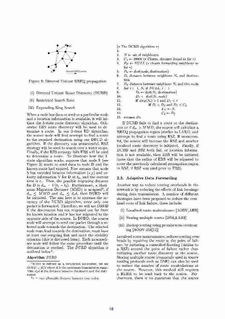
çM·LÉIÒ½f¼ ÏÆ(ÀÁ¾½fÆIÅLÅ¼Ñ KÆ£ÆZÑZ·LÀÉñÒK¸¿·LÀÉñ¼ÔáZºK»IÀKÑZ·LÀɽf·ÀKÉ¥¸¾¼B»I½fÓ¶

¼BÀKÓÔ¼ØÇz¼¡ÁÃϼB¼¡À-Áf¶¼lÁÃãƳ·¹¸Ü·LÀÁf¶¼lû˥½¾Æ(ÒZÁ¾¼¸Ï»I½¾¼lÓ¡½¾¼¡Ì»#Á¾¼BÑ»IÀKÑÒK¸¿¼ÑTßýÊZÚå·¹¸hÇK»(¸¿¼ÑÆIÀ¸¿Æ(Ò½ÂÓÔ¼-½fÆIÒZÁf·ÀÉzÕ趷¹Ó¶'ͼ»#ÀK¸BÕR¼B»(Ó¶'Ñ»#Áf»!ºK»IÓÂÞ(¼ÔÁ¥ÓB»#½f½¾·L¼B¸³Á¾¶¼Ó¡ÆI̺ͥÅL¼ÔÁf¼¸¾ÆIÒK½fÓ¡¼Á¾ÆÑZ¼¸Áf·ÀK»#Á¾·LÆIÀ »IÑÑZ½f¼B¸f¸Bß×læý¨þ ·¹¸»ºDÆI·LÀÁ¿Ì^Á¾Æ#Ì¢ºDÆI·LÀ(Á½fÆIÒZÁf·ÀKɺK½¾ÆIÁ¾ÆZÓÔÆ(ÅnÕ>趷¹Ó¶ͼB»#Àz¸vÁ¾¶K»#ÁÁf¶¼1Ñ»#Áf»-ºK»(ÓÂÞI¼¡Áf¸¨Æ(ÀÅËÓ¡»I½¾½fË-Áf¶¼1À¼¡á£Ál¶ÆIº»(ÑÑZ½f¼B¸f¸»IÀKÑØÁ¾¶¼ãÑZ¼B¸¿Á¾·LÀK»>Áf·Æ(À³»IÑѽ¾¼¸¾¸Bß@×À£ÒÍaÇz¼B½@Æ Û ÑZ·ör¼¡½f¼¡ÀÁ¸¿Á¾½Â»>Áf¼¡ÉI·L¼B¸Ï¶K»Ù(¼ØÇD¼¡¼BÀºK½¾Æ(ºzƸ¿¼Ñ-Á¾Æ½f¼BÑZÒzÓÔ¼ØÁ¾¶¼h½fÆIÒZÁ¾Ì·LÀɯÆ>Ù(¼¡½f¶¼B»(ѸÝÆ Û ºÒ½f¼ KƣƣѷÀÉzß³µÃÏƸ¿ÒzÓ¶!¸¿Á¾½Â»>Á¾¼¡ÌÉ(·¼¸³»#½f¼IÕMôáZºK»#ÀzÑZ·ÀKÉÚ¨·ÀKÉ!Ê£¼B»I½fÓ¶ÎôÏÚlÊÐh»IÀKÑÚ¨¼¡Ì¸¿Á¾½f·LÓÔÁ¾¼ÑÊ£¼»#½ÂÓ¶ DÆ(À¼B¸ÎnÚlÊTÐÔßäeÀôÏÚlÊrÕTÁf¶¼-¸¿Æ(Ò½ÂÓÔ¼ÀÆZÑZ¼Ø·ÀzÓÔ½f¼¡Í¼¡ÀÁf»IÅÅLË·ÀzÓÔ½f¼B»I¸¾¼B¸RÁ¾¶¼`¸¾¼B»#½ÂÓ¶-»#½f¼B»hÒKÀ(Áf·ÅÁf¶¼-¼¡ÀÁ¾·L½f¼-À¼ÔÁÃãÆI½fÞ·L¸1¸¿¼»#½ÂÓ¶¼BÑ!ÆI½`Áf¶¼ÑZ¼B¸¿Á¾·LÀK»#Á¾·LÆIÀ¶K»(¸ÝÇD¼¡¼BÀ Û ÆIÒÀzÑTßØçKÆI½l¼¡á»#ͺÅL¼IÕD· Û ÀKƣѼ¥ÊÎn¸¿¼B¼1çM·ÉIÌÒ½f¼ ÐRû#ÀÁf¸RÁ¾Æ1÷KÀKѯ»1½¾Æ(ÒZÁ¾¼ÝÁ¾Æ¥ÀÆZÑZ¼Ø×1Õ·ÁÏè·LÅLÅrÓ¡½¾¼¡Ì»#Á¾¼-»ªÚlÚÝô ú ºK»IÓÂÞ(¼ÔÁ`è·Áf¶»µ·LͼµdÆÖ·LÙI¼Îµ¨µ¨ÖMÐÆ Û ÆIÀ¼(Õ趷LÓ¶sͼB»#Àz¸³Áf¶K»>ÁÆIÀÅLËÁ¾¶¼À¼B·É(¶ÇDÆIÒK½¾·LÀÉÀÆZÑZ¼¸¥ÕØÕç9»IÀKÑè·LÅŨ¸¾¼¡¼¯Á¾¶¼ºK»IÓÂÞ(¼ÔÁßólÆ>ÃhÕ¸¾·ÀzÓÔ¼1ÀKƣѼB¸ç »IÀKÑX¶K»Ù(¼1»ÅL·LÀÞÁ¾ÆÀÆZÑZ¼a×1ÕzÁf¶¼¡ËÓB»#À¸¿¼BÀKÑÇK»IÓÂÞ»ÚÝÚÝôÏÈFÁfÆÀÆZÑZ¼¯ÊrßM×l¸³»½f¼B¸¾ÒÅÁ1»½fÆIÒZÁf¼Çz¼¡ÁÃϼB¼¡ÀÀÆZÑZ¼¯Ê»#ÀKÑÀÆZÑZ¼× Ó¡»#ÀÇD¼¼B¸¿Áf»IÇZÌÅL·L¸¾¶¼Ñhè·Áf¶ÆIÒÁKÆ£ÆZÑZ·LÀÉÝÁf¶¼Ü¼BÀ(Áf·½f¼ÜÀK¼ÔÁÃãÆI½fÞDßTä Û ÀÆZÑZ¼× Ãã»(¸lÍÆI½f¼hÁf¶K»>Á`ÆIÀ¼a¶ÆIº!»Ãã»Ë(ÕÁ¾¶K¼¡ÀÀKƣѼ¥Êè·LÅLÅÁf·Í¼¡Æ(ÒZÁÝ· Û ÀƽfÆIÒZÁf¼`½¾¼BºÅ˯·L¸½f¼BÓ¡¼¡·LÙI¼BÑ»#ÀzѯÉ(¼¡À¼B½f»#Á¾¼»IÀÆ#Áf¶¼¡½³ÚÝÚlô ú ºz»IÓÂÞI¼¡Áhè·Áf¶»¶K·É(¶¼¡½³µ¨µ¨ÖÙ>»#ÅLÒ¼(ßäeÀÚlÊMÕ£ÉI·LÙI¼BÀ-Á¾¶z»>ÁãÁ¾¶¼`¸¿Æ(Ò½ÂÓÔ¼lÀKƣѼضK»(¸Ï¸¾ÆIͼطLÑZ¼»Æ Û Á¾¶K¼lÓÔÒ½f½f¼¡ÀÁÅÆZÓ¡»#Á¾·LÆIÀ¥Æ Û Á¾¶¼ÝѼB¸¿Á¾·LÀK»>Áf·Æ(À¥Æ(½Þ£ÀÆ>Ãݸ»Iºº½fÆ᣷LÍ-»>Áf¼¡ÅL˶Æ>ÃåÍ»IÀ£Ë¶Æ(ºK¸³»Ã»Ë·Áa·L¸BÕd·ÁaÓB»#ÀÓB»#ŹÓÔÒŹ»>Áf¼¯»½f¼¡ÉI·LÆIÀ·LÀ趷¹Ó¶Áf¶¼ªÑZ¼¸Áf·Àz»>Á¾·LÆIÀ'ÀÆZÑZ¼ÓB»#ÀÓ¡Ò½¾½f¼¡ÀÁfÅ˽f¼B¸¾·LÑZ¼¥»#ÀKÑKÆ£ÆZÑè·Á¾¶·LÀÁf¶K»>Á`½¾¼BÉI·LÆIÀÆ(ÀÅË(ß@µÃãÆݸ¿ÒKÓ¶`º½fÆ#ÁfÆZÓÔÆIŹ¸r趷¹Ó¶hÒK¸¾¼RÚlÊ¥»#½f¼Ö@×ØÚ »IÀKÑÚÝýØò×lÚhßãäeÀÖ@×ØÚ IÕ¨· Û Á¾¶¼!¸¿Æ(Ò½fÓ¡¼ÀÆZÑZ¼¶K»(¸»ÅLÆ£ÓB»>Áf·Æ(À·LÀ Û Æ(½¾Í-»>Áf·Æ(À Î Á¾¶½fÆIÒKÉI¶»Ä`ÈÏÊÐ`»IÇzÆ(ÒZÁ1»ºK»I½¿Áf·LÓ¡ÒŹ»#½-ÀÆZÑZ¼(Õ¨·ÁªÓB»#ÀÓ¡»IÅLÓ¡ÒŹ»>Á¾¼»½¾¼BÉI·LÆIÀÓ¡»#ÅLÅL¼BÑÁf¶¼ØôR᣺D¼BÓÔÁ¾¼Ñ DÆIÀ¼(Õ(·LÀ趷¹Ó¶-Áf¶¼ØÑZ¼¸Áf·Àz»>Á¾·LÆIÀ¯ÀÆZÑZ¼ÓB»#À ½¾¼¸¿·¹ÑZ¼Ißä Û Áf¶¼¸¿Æ(Ò½ÂÓÔ¼ÀÆZÑZ¼·¹¸-ÆIÒZÁ¸¿·¹ÑZ¼Æ Û Áf¶¼ôR᣺D¼BÓÔÁ¾¼Ñ rÆIÀ¼(Õ(»hÚ¨¼3(ÒK¼B¸¿ÁQDÆIÀK¼³Î 趷¹Ó¶-·L¸Ï»`½¾¼BÉI·LÆIÀ¸¾Ò½f½¾Æ(ÒÀKÑZ·LÀÉ`Á¾¶K¼Ø¼¡á£ºD¼BÓÔÁ¾¼Ñ-è¡Æ(À¼ÐR·L¸ã»#Ź¸¿ÆaÓ¡»#ŹÓÔÒKÅL»#Á¾¼BÑß

Request ZoneExpected Zone

S

D

(a) Localized RREQ propagation in LAR1

RREQ packet

S D

(b) Localized RREQ propagation in RDMR

Relative Distance in hops H = 1

çM·É(Ò½f¼ ÏÆ(À(Áf½¾Æ(ÅÅL¼BÑ KÆ£ÆZÑZ·ÀKÉ<ÒK¸¾·LÀÉå½¾¼¸Áf½¾·¹ÓÁf¼BѸ¾¼B»#½ÂÓ¶¯èBÆIÀ¼

µ¶¼Ü¸¾ÆIÒK½fÓ¡¼ÀÆZÑZ¼Rè·LÅÅIÁ¾¶¼BÀ³½¾¼¸Áf½¾·¹ÓÁ@ÚlÚÝô ú ºK»IÓÂÞ(¼ÔÁTÁfÆÁ¾¶K¼-ÀÆZÑZ¼B¸hè·Á¾¶K·ÀÁf¶¼½f¼Ò¼B¸¿Áhè¡Æ(À¼-ÆIÀÅLËsÎn¸¿¼B¼çM·ÉIÌÒ½f¼ #»ÐßäeÀ'ÚlýØò×ØÚhÕMÁ¾¶¼¸¿Æ(Ò½ÂÓÔ¼-ÀÆZÑZ¼¸³¼B¸¿Á¾·LÍ-»>Áf¼Á¾¶K¼aÀ£ÒÍaÇz¼B½Æ Û ¶Æ(ºK¸lÁ¾¶¼-ÑZ¼¸Áf·ÀK»#Á¾·LÆIÀ!·L¸`»Ã»Ë Û ½fÆIÍ·Á¨În»I¸f¸¿ÒKÍ¥·LÀÉh»ÍƣѼ¡½Â»>Á¾¼ãÙI¼BÅÆZÓ¡·ÁËÐÕ#Á¾¶£ÒK¸v½f¼B¸¿Á¾½f·LÓÔÁ¾·LÀÉÁ¾¶K¼³½¾Æ(ÒZÁ¾¼³Ñ·L¸fÓÔÆ>Ù(¼¡½fËè·Áf¶·LÀÁ¾¶¼1ÓB»#ŹÓÔÒŹ»>Áf¼BÑÀ£ÒÍ1ÇD¼¡½Æ Û ¶ÆIºÎn¸¿¼B¼`çM·LÉIÒ½f¼ >ÇzÐÔß

ë ë < ° )& )3$² /60)3$ï+-23(4/5,.$'7b+-8B:°;)7b& )$5:×l¸@ÑZ·L¸fÓÔÒz¸¾¸¾¼BѼB»I½¾ÅL·L¼¡½ÕBÖ@ÈT×ØÚ·L¸d»ºzÆ(·ÀÁ¿Ì^Á¾ÆIÌ^ºDÆI·LÀÁTÇK»I¸¾¼BѽfÆIÒZÁf·ÀÉ!¸Áf½f»#Á¾¼¡É(ËIÕM趷¹Ó¶¶K»I¸1Çz¼B¼¡ÀÇÒK·ÅÁaÆ(ÀÁ¾Æ(ºÆ Û×læý¨þaßÝùÝÆ>Ã㼡ÙI¼B½BÕl·À9Ö@ÈT×ØÚhÕ¨¼B»(Ó¶FÀÆZÑZ¼»IÅL¸¾Æs¼¡á£ÌÓ¶K»IÀÉI¼¸ØÅLÆZÓ¡»#Á¾·LÆIÀ·À Û Æ(½¾Í-»#Á¾·LÆIÀÎ ÒK¸¾·ÀKÉÄ`ÈÏÊ!ÓÔÆ£ÆI½ÂÑZ·ÌÀK»#Á¾¼B¸ÂÐ@·À1Á¾¶¼B·½v¶¼BÅÅLÆØͼ¸¾¸f»#É(¼ÜÇD¼B»IÓ¡ÆIÀ·LÀÉzß@äeÀaÖdÈT×lÚhÕ· Û »ÀÆZÑZ¼-¶K»(¸`ÅÆZÓB»>Á¾·LÆIÀ·LÀ Û ÆI½fÍ-»>Á¾·LÆIÀ Û Æ(½³»ª½f¼Ò·L½f¼BÑÑZ¼¸Áf·ÀK»#Á¾·LÆIÀÕØ·Áè·LÅÅ`ÒK¸¾¼!ÑZ·ör¼¡½f¼¡ÀÁ½fÆIÒÁ¾¼!Ñ·L¸fÓÔÆ>Ù(¼¡½f˸¿Á¾½Â»>Á¾¼BÉI·L¼B¸ÏÁ¾Æ-ÑZ¼¡Á¾¼B½¾Í·LÀ¼h»a½fÆIÒÁ¾¼IÕZÑZ¼Bºz¼BÀKÑZ·LÀÉ-ÆIÀªÁ¾¶K¼½f¼BÓÔÆ(½¾¼ÑÅLÆ£ÓB»>Áf·Æ(À »IÀKÑ'Ù(¼¡ÅLÆZÓÔ·ÁËÆ Û Á¾¶¼ÑZ¼¸Áf·ÀK»#Á¾·LÆIÀßµ¶¼»I·Í0Æ Û ÆIÒK½à>Ìe¸Á»>Á¾¼½fÆIÒÁ¾¼ÑZ·¹¸¾Ó¡Æ>ÙI¼B½¾Ë'¸¿Á¾½Â»>Áf¼¡É(Ë·¹¸Á¾ÆÍ·LÀ·Í·¹¸¿¼½¾Æ(ÒZÁ¾·LÀÉÆ>ÙI¼B½¾¶¼»IÑ'·ÀÁ¾½fÆZÑZÒKÓ¡¼BÑ ·ÀÁfÆÁ¾¶K¼ØÀ¼¡ÁÃÏÆ(½¾Þ Û ÆI½ã¼B»(Ó¶-½¾Æ(ÒZÁ¾¼ÑZ·¹¸¾Ó¡Æ>ÙI¼¡½fËIÕ(趷Lż`¸¿¼BżÓÁ¾Ì·LÀɳ½f¼¡Å¹»>Á¾·LÙI¼BÅ˸¿Áf»#ÇKżݽfÆIÒÁ¾¼B¸Øε¶·¹¸Ïè·ÅLÅzÇD¼ØÑ·L¸fÓÔÒK¸f¸¾¼BÑŹ»>Á¾¼B½ÂÐÔß ¼Ý¶K»Ù(¼¨ÑZ¼Ô÷KÀK¼BÑ-àhÑZ·öD¼B½¾¼BÀÁܽ¾Æ(ÒZÁ¾·LÀɳ¸fÓÔ¼BÀK»#½¾Ì·LÆ(¸R»IÀKÑÑZ¼B¸fÓÔ½f·ÇD¼¨Ã¨¶K»#ÁϸÁf½f»#Á¾¼BÉI·L¼B¸»#½f¼¨ÒK¸¾¼BÑaÁ¾ÆaÑZ¼ÔÁf¼¡½¾ÌÍ·ÀK¼¥»ª½¾Æ(ÒZÁ¾¼ Û ÆI½¼B»(Ó¶!¸fÓÔ¼¡Àz»#½f·Æzßùl¼¡ÀKÓ¡¼IÕrÁ¾¶K¼aÀK»Iͼà>Ìe¸¿Áf»>Áf¼a½fÆIÒÁ¾·LÀÉKßµ¶¼½fÆIÒZÁf·ÀKÉÑ·L¸fÓÔÆ>Ù(¼¡½f˸Áf½f»#Á¾¼¡É(·¼¸ÒK¸¾¼BѪ·ÀÆ(Ò½Ýà>Ìe¸Á»>Áf¼`»IÅÉ(ÆI½f·Áf¶Íø»#½f¼h»I¸ Û Æ(ÅÅLÆ>Ãݸ

D

S Directed RREQ packet

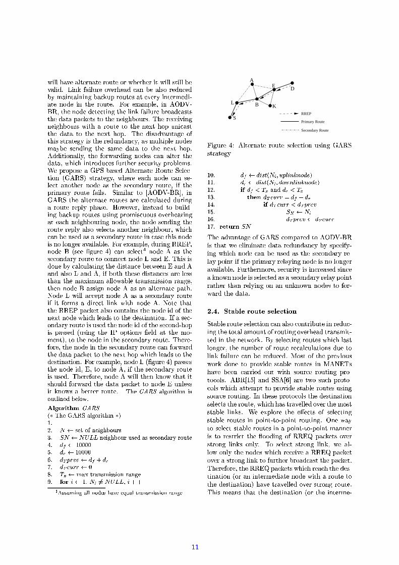
çM·É(Ò½f¼`à ýl·L½¾¼ÓÁf¼BÑõÝÀ·¹Ó¡»(¸ÁlÚlÚÝô ú º½¾Æ(ºK»#É»>Áf·Æ(À

Î · Ðýl·L½¾¼ÓÁf¼BÑõÝÀ·¹Ó¡»(¸ÁÝÚ¨Æ(ÒZÁ¾¼³ýØ·¹¸¾Ó¡Æ>ÙI¼¡½fËÎýõlÚlýÐη· ÐÚ¨¼B¸¿Á¾½f·LÓÔÁ¾¼ÑÊZ¼B»#½ÂÓ¶ rÆIÀ¼Î ·L·· ÐôáZºK»#ÀzÑZ·ÀKÉÚÝ·ÀÉÊ£¼»#½ÂÓ¶¶¼BÀa»lÀÆZÑZ¼Ü¶K»(¸dÑK»>Áf»ÝÁ¾Æ¸¿¼BÀKÑ`Á¾Æ`»Ýºz»#½¾Á¾·¹ÓÔÒŹ»#½dÀÆZÑZ¼»IÀKѯ»aÅÆZÓB»>Á¾·LÆIÀª·À Û ÆI½fÍ»#Á¾·LÆIÀª·L¸»Ù>»#·LÅL»IÇÅL¼IÕ·Á¨Ã¨·LÅÅT·LÀ·ÌÁf·L»#Á¾¼aÁ¾¶¼à>Ìe¸Á»>Áf¼1½fÆIÒZÁf¼aÑZ·¹¸¾Ó¡Æ>ÙI¼B½¾Ë»#ÅLÉIÆ(½¾·Á¾¶Íß1ælÁ¾¶Ì¼B½¾Ã¨·¹¸¿¼!ôÜÚlʽ¾Æ(ÒZÁ¾¼ÑZ·L¸fÓÔÆ>Ù(¼¡½fËsè·LÅLÅÇD¼ÒK¸¿¼ÑÁfÆsÑZ¼¡ÌÁf¼¡½fÍ¥·LÀ¼»½fÆIÒZÁf¼Iß äeÀXÆIÒ½à>Ìe¸¿Áf»>Áf¼!ÚÝý »IÅÉ(ÆI½f·Áf¶ÍÕÁf¶¼a¸¾ÆIÒ½ÂÓÔ¼1ÀÆZÑZ¼aè·LÅLÅ@÷K½Â¸¿Á`»#Á¿Á¾¼BͺZÁØÁfÆ÷KÀzÑ»-½fÆIÒZÁf¼ÁfÆÁf¶¼½¾¼3(ÒK·½f¼BÑsÑZ¼B¸¿Á¾·LÀK»>Áf·Æ(À'ÒK¸¾·LÀÉ!Æ(Ò½-ýØÚõØý »#ÅÌÉ(ÆI½f·Áf¶Íߪä Û Á¾¶K¼ªÑZ·¹¸¾Ó¡Æ>ÙI¼B½¾ËûI¸hÒKÀK¸¿ÒzÓ¡ÓÔ¼¸¾¸ Û ÒÅ^ÕÚlʸ¿Á¾½Â»>Áf¼¡ÉIË1è·ÅLÅzÇD¼ÝÒK¸¾¼BÑ¥ÁfÆ1¸¾¼B»#½ÂÓ¶Æ>ÙI¼B½R»hè·LѼ¡½Ü¸fÓÔÆ(ºz¼(ßçM·LÀK»#ÅLÅË(Õ(· Û Á¾¶K¼ØÚ`TʸÁf½f»#Á¾¼¡É(Ë Û »I·Å¹¸ÏôÏÚlʥè·LÅÅDÇz¼ØÒK¸¾¼BÑÁfÆsÑZ¼¡Á¾¼¡½fÍ·ÀK¼»'½¾Æ(ÒZÁ¾¼(ßµdÆ'·LÅÅLÒK¸¿Á¾½Â»>Áf¼¶Æ>à Áf¶¼à#̸¿Áf»#Á¾¼¯»IÅÉ(ÆI½f·Áf¶Í ÃãÆI½fÞZ¸¡ÕM¸¿ÒºKºzƸ¿¼-Áf¶K»>Á¥ÀÆZÑZ¼ªÊÎn¸¿¼B¼çM·LÉIÒ½f¼¥àÐØÃã»IÀ(Á¸Á¾Æ¸¾¼¡ÀKÑÑ»>Á»ÁfÆÀÆZÑZ¼-ý »#ÀKÑ!Áf¶¼Þ£ÀÆ>èÀª½¾Æ(ÒZÁ¾¼`¶K»(Ѫ¼¡áZº·½f¼BÑßvólÆ>û(¸¾¸¾ÒͼÁ¾¶K»#ÁÝÀÆZÑZ¼Ê¯¶K»I¸½f¼BÓ¡ÆI½ÂÑZ¼BѪÅLÆ£ÓB»>Áf·Æ(À¯·LÀ Û ÆI½fÍ-»>Á¾·LÆIÀÎ áTÕ Ëл#ÀKÑÙI¼¡ÌÅLÆZÓÔ·Á˪·LÀ Û ÆI½fÍ-»>Áf·Æ(Àþ Û Æ(½Øýå»>Á ÕT»#ÀzÑÁ¾¶¼ÓÔÒK½¾½f¼¡ÀÁÁf·Í¼¥·L¸ ! ßhµ¶¼BÀÕDÁ¾¶¼¥ºzƸ¾¸¾·LÇżaÍ·É(½f»#Á¾·LÀɯÑZ·¹¸Á»#ÀKÓ¡¼Û Æ(½³ý ·L¸Î ! ÐÔßçÒ½¾Á¾¶K¼¡½fÍ¥Æ(½¾¼(Õ@»ò»>áZ·ÌÍaÒÍ ò·LÉI½Â»>Áf·Æ(ÀýØ·L¸¿Áf»IÀKÓÔ¼Înòòý`Ð`·L¸1»I¸f¸¿·LÉIÀ¼ÑÕ@· Û »IÀKÑ KÕlÁ¾¶¼BÀýõlÚÝý è·LÅLÅÇD¼-·ÀK·Áf·L»#Á¾¼BÑ߯µ¶¼»#·LÍ ¶¼B½¾¼-·¹¸Á¾Æ·LÀKÓ¡½¾¼»I¸¾¼aÁf¶¼»IÓÔÌÓ¡Ò½f»(ÓÔËÆ Û Á¾¶¼ýõlÚÝýâ»#ÅLÉIÆI½f·Á¾¶ÍÕظ¾·LÀKÓÔ¼ÆIÀKÅËÆ(À¼ºK»(ÓÂÞI¼¡Ád·¹¸ Û Æ(½¾Ã»#½ÂÑZ¼ÑTß@µ¶¼B½¾¼ Û ÆI½f¼IÕÃϼãè·LÅÅZÒK¸¾¼ýØÚõlý· Û Á¾¶¼ÑZ¼B¸¿Á¾·LÀK»#Á¾·LÆIÀ¶K»(¸1ÀKÆ#ÁaÍ·LÉI½Â»>Áf¼BÑÁ¾Æ£Æ Û »#½ Û ½fÆIÍ·Áf¸Þ£ÀÆ>èÀªÅÆZÓ¡»#Á¾·LÆIÀ»#ÀKѯ·ÁݶK»(¸ãÀÆ#Á¨Í·É(½f»#Á¾¼Ñ-Á¾Æ¥Áf¶¼Æ(ººzƸ¿·Á¾¼h¸¾·LÑ¼Æ Û Áf¶¼³¸¾ÆIÒ½ÂÓÔ¼(ßdäeÀýõlÚÝýaÕÁf¶¼³¸¿Æ(Ò½ÂÓÔ¼ÀÆZÑZ¼Ïè·ÅLÅZ»>Á¾Á¾¼¡ÍºZÁMÁ¾Æ¸¿¼BÀKÑhÆ(À¼ÜºK»(ÓÂÞI¼¡Á@Á¾¶K½¾Æ(ÒÉI¶1»Ø¸¿¼¡ÌÅL¼BÓÔÁ¾¼BÑÀÆZÑZ¼lÁfÆ>Ãã»I½fÑK¸vÁ¾¶¼`ÑZ¼¸Áf·ÀK»#Á¾·LÆIÀßµ¶¼¸¿¼BżÓÁf¼BÑÀÆZÑZ¼ÍaÒK¸¿Á@ż»IÑØÁ¾Æ>û#½ÂѸDÁf¶¼ÜÑZ¼¸Áf·ÀK»#Á¾·LÆIÀÕÍ1Òz¸Á@¶z»ÙI¼»#Á`ÅL¼B»(¸ÁhÆ(À¼ÆIÒZÁfÉIÆI·LÀÉÅ·LÀÞ»#ÀKÑ!ͼ¡¼ÔÁhÁf¶¼¸¿Áf»#ÇK·ÅL·ÁËÓ¡½¾·Á¾¼B½¾·LÆIÀÎ Á¾¶·¹¸ã·L¸ãÑZ·¹¸¾Ó¡ÒK¸¾¸¾¼BÑÅL»#Á¾¼¡½ÐßvôÜ»(Ó¶-·ÀÁf¼¡½fÍ¥¼ÑZ·Ì»#Á¾¼hÀÆZÑZ¼³Ã¨·LÅLÅ Û Æ(ÅÅLÆ>ÃFÁf¶¼a¸f»#ͼhº½fÆZÓÔ¼ÑZÒ½f¼hÒÀÁ¾·LÅ@Áf¶¼ÑZ¼¸Áf·Àz»>Á¾·LÆIÀ·¹¸a½¾¼»IÓ¶¼ÑTßµ¶¼ !,»#ÅLÉIÆ(½¾·Á¾¶Í,·¹¸Æ(ÒZÁ¾ÅL·ÀK¼BѪÇz¼BÅÆ>Ã!"Iß#%$'&()+*-,. /0213405766[@ GcJFA8bEADF ZLc=Z"cGU:9P Z MGIE CZ7;aZLUVASMA<;>= \;A c9ADM

??@BADCFE i \OA<;AHG Gc4MO3A6U ZJIGUK9U"ML;ZLEcUVGc9cGIEM;ZLEHANO Pc9IP=RQTSUQ Gc6M9OA FGc-MaZLE3_ABW4ASMY\;ADADE`M9OA c9I9P;_DABZLEFVMOABFADc9M9G VEbZ M9GIEW7X A U ZJI ZLPPI\ ZLWPA FGc-MaZLE_DA W*ASMY\;ADAE MY\NIQEI FADc

Y[Z]\M^`_badcKefahg+ikjmlmn<oqp<^rsZ+tuRvwxvyz| _Jp4lm~`_7ojR^xlRn |vdzu7RRm Y[Zil | _ | pd`o | p>gm`7_d~lm | l~gTndZmt vzyK Y[Z U^`l | _7%~lmnMg+n>ok`j_7ojR^xlm`n | l

~g+nbZmtxv bz¡£¢L¤J¥ Y¦¨§ ¡x©Pª¡x©+¤J¥«¢ ¦¬ ¥L¢ §m¦Ht­v ]® `o | p>gm`7_¯_UpLM_J_7°_7ojR^xlm`n y!® g+°`_ | p<okg+±

p<olm²xv ³ `o | p>g+7_:_JpL_7_7´_7ojR^xlm`n y ® gmp<^o | lx_µv¶ () ¢z·uR¸y ®4¹º yKF»¸¢¼½¼¾v ]®z¡£¢L¤J¥ Y y ®ª¡x©+¤J¥«¢ ¦¬ ¥«¢ §m¦Htuxv ³ z¡£¢[¤7¥ Y y!®ª ¦¨§ ¡x© tuRumv * ¶K ©7¿ Y y ® t»À u g+ ³ÁÃÂuTw£v * ¶K ]® Á ] gm ³Á uxv BzÄy ®u v zÄ ³uT£v )TÅx,ÆÇ)+È Éä Û ýØõØÚÝý Û »I·Å¹¸`ÁfÆ÷KÀKÑ»½fÆIÒZÁf¼Á¾ÆÁ¾¶K¼¯ÑZ¼B¸¿Á¾·LÀK»#Ì

Á¾·LÆIÀªÆI½ã· Û ÊË ÕÁ¾¶K¼¸¾ÆIÒ½ÂÓÔ¼Øè·ÅLÅTÓ¡»IÅLÓ¡ÒÅL»#Á¾¼`»ÚÝÚÝô ú º½fÆIºz»#É(»#Á¾·LÆIÀa½¾¼BÉI·LÆIÀθ¾·Í·LÅL»I½vÁ¾Æ³Ö@×ØÚ ÐÔÕ(»IÀKÑ»>Á¾Á¾¼BÍ¥ºÁhÁ¾Æ÷KÀKÑ»½¾Æ(ÒZÁ¾¼ÒK¸¾·LÀÉÚlÊMßTä Û ÒÀK¸¾ÒKÓBÓÔ¼B¸f¸¿ÌÛ ÒÅ^ÕKÁf¶¼a¸¾ÆIÒK½fÓ¡¼hè·ÅLÅd·LÀKÓ¡½¾¼»I¸¾¼`Á¾¶¼¥ÚlÊ»#ÀzÑ»#ÀÆIÁ¾¶¼B½ÅLÆ£ÓB»#ÅL·L¸¾¼BÑs½fÆIÒZÁf¼ÑZ·L¸fÓÔÆ>Ù(¼¡½fË·L¸·À·Á¾·¹»>Áf¼BÑTßñçM·Àz»#ÅLÅË(Õã· ÛýõlÚÝý »#ÀzÑÚlÊÇDÆ#Á¾¶ Û »#·LÅnÕÝÆ(½ÅLÆ£ÓB»>Áf·Æ(À·À Û Æ(½¾Í-»#ÌÁ¾·LÆIÀs·L¸ÀKÆ#Á»Ù>»#·LÅL»IÇż(ÕvÁ¾¶¼BÀ ôÏÚlÊ'è·ÅLŨÇz¼·LÀ·Á¾·¹»>Á¾¼ÑÎ ÀKÆ#Á¾¼¥Áf¶K»>ÁhÁf¶¼½f»(ÑZ·Òz¸`Æ Û ôÏÚlÊè·ÅLÅÇz¼»(ÑPÌÒK¸¿Á¾¼ÑÁfÆÓÔÆ>Ù(¼¡½@Á¾¶¼ãº½f¼¡Ù£·Æ(ÒK¸¾ÅË`Ó¡»IÅLÓ¡ÒÅL»#Á¾¼Ñhº½fÆIºK»IÉ(»>Áf·Æ(À`½¾¼BÉI·LÆIÀ·LÀÚØÊMÕZ· Û ÚlÊ.ûI¸Òz¸¿¼Ñ¯º½f·LÆI½Á¾Æ-ôÏÚlÊÐß

ë @ë ­ÎÍ1&ÏB)+-,.$ï& )3&ÃÐ1/7PÑ &<7PÍB+-8B:×ÝÀKÆ#Á¾¶K¼¡½¥Ãã»Ë!Á¾Æ!½¾¼ÑZÒKÓÔ¼¯½¾Æ(ÒZÁ¾·LÀÉÆ>Ù(¼¡½f¶¼B»(Ѹ`·LÀÁ¾¶K¼À¼¡ÁÃÏÆ(½¾Þa·L¸ÜÇË¥½f¼BÑZÒKÓ¡·ÀKÉhÁ¾¶¼l¼Ôör¼BÓÁ¸ÜÆ Û Å·LÀÞǽf¼B»#Þ>»IÉI¼ÑZÒ½f·LÀÉÑ»>Á»Á¾½Â»#ÀK¸¾Í·L¸f¸¿·LÆIÀ@ß×øÀÒKÍ1ÇD¼¡½hÆ Û ÑZ·öD¼B½¾¼BÀÁ¸¿Á¾½Â»>Á¾¼BÉI·L¼B¸ã¶K»Ù(¼ØÇD¼¡¼BÀºK½¾Æ(ºzƸ¿¼Ñ-Á¾Æ-½f¼BÑÒKÓÔ¼ØÁ¾¶¼hÆ>Ù(¼¡½¾Ì¶¼»IÑÓÔÆ(¸¿Áf¸Æ Û ÅL·LÀÞ Û »#·LÅLÒ½¾¼(ÕZÁ¾¶K¼B¸¾¼·LÀKÓ¡ÅÒKѼ Î · ЪÖ@ÆZÓ¡»#ÅL·¹¸¿¼Ñ½fÆIÒZÁf¼Í-»I·ÀÁf»I·Àz»#ÀKÓ¡¼¥ÿ ×læý¨þ1Õ × Ú Î ·L· ÐÊ£Á¾ÆI½f·LÀÉÍ1ÒÅÁ¾·LºÅL¼h½¾Æ(ÒZÁ¾¼¸hÿ ý`ÊZÚhÕ Ö@×ØÚ Î··L· Ð »(ÓÂÞÒKºh½¾Æ(ÒZÁ¾·LÀÉlÒz¸¿·LÀÉlºK½¾Æ(Í¥·¹¸fÓÔÒÆ(ÒK¸TÆ>ÙI¼B½¾¶K¼B»#½¾Ì

·LÀÉÿ ×læý¨þÝÌ Ú³ÿ ÖÆZÓB»#ÅL·L¸¾¼BÑؽ¾Æ(ÒZÁ¾¼Í-»I·ÀÁf»I·Àz»#ÀKÓ¡¼IÕ¡½f¼BÑÒKÓÔ¼¸T½¾Æ(ÒZÁ¾·LÀɨÆ>Ù(¼¡½¾Ì¶¼»IѸǣ˽f¼¡ºK»I·½f·ÀKɯÁf¶¼-½¾Æ(ÒZÁ¾¼»>Á`Áf¶¼-ºzÆ(·ÀÁhÆ ÛÏÛ »#·LÅÌÒ½f¼IÕZǣ˯·LÀ·Á¾·¹»>Áf·ÀÉ»-Ó¡ÆIÀÁ¾½fÆIÅLÅL¼BÑ zÆÆZÑZ·LÀÉÎn¸¿·LͷŹ»#½ÁfÆ»'ÚØÊTлI½¾Æ(ÒÀKÑ Áf¶¼!ºDÆI·LÀÁªÆ ÛhÛ »#·LÅÒ½f¼½Â»>Áf¶¼¡½¯Á¾¶K»IÀ·LÀ·Áf·L»#Á¾·LÀÉ»#ÀÆIÁ¾¶¼B½-½¾Æ(ÒZÁ¾¼ÑZ·¹¸fÓÔÆ>ÙI¼B½¾Ë»#Á¥Áf¶¼¸¾ÆIÒ½ÂÓÔ¼(ßÊÁfÆI½f·ÀÉ1Í1ÒÅÁ¾·LºÅL¼Ø½fÆIÒZÁf¼B¸ØÎÓÔÆ(ÍÍ¥Æ(ÀÅLË¥Òz¸¿¼Ñ-·Àª¸¿Æ(Ò½fÓ¡¼½fÆIÒZÁf·Àɺ½fÆ#ÁfÆ£Ó¡ÆIŹ¸Ø¸¾ÒKÓ¶»I¸`ýÊÚlÐ`Ó¡»IÀ!»#Ź¸¾ÆªÇD¼ÒK¸¿¼ÑÁ¾Æ½f¼BÑÒKÓÔ¼Áf¶¼À£ÒÍaÇz¼B½Æ Û ½fÆIÒZÁf¼½¾¼Ó¡»#ŹÓÔÒKÅL»#Á¾·LÆIÀK¸-»#ÁÁ¾¶K¼!¸¾ÆIÒ½ÂÓÔ¼(ßñùlÆ>ÃϼBÙI¼B½BÕÏÁ¾¶·¹¸ªÍ¥¼¡Á¾¶ÆZѸ¿Á¾·LÅLÅl½f¼Ò·L½¾¼¸»ÚÝôÏÚÝÚ,Á¾ÆÇD¼'¸¾¼¡ÀKÑñÇK»(ÓÂÞÁ¾ÆÁ¾¶¼'¸¾ÆIÒK½fÓ¡¼Iß çKÒ½¿ÌÁ¾¶K¼¡½fÍ¥Æ(½¾¼(ÕRÁf¶¼¡½f¼·L¸ÀÆÉIÒK»I½f»IÀÁ¾¼¡¼ªÁ¾¶z»>Á-Á¾¶K¼¸¿Æ(Ò½fÓ¡¼

è·LÅÅz¶K»ÙI¼Ø»#ÅÁ¾¼¡½fÀK»#Á¾¼¨½fÆIÒZÁf¼ÝÆI½Ï趼ÔÁf¶¼¡½Ï·Áãè·ÅLÅD¸¿Á¾·LÅLÅKÇD¼Ù>»#ÅL·¹ÑTߪÖ@·ÀÞ Û »#·LÅÒK½¾¼-Æ>Ù(¼¡½f¶¼B»(ÑÓ¡»IÀÇz¼¯»IÅL¸¾Æ½¾¼ÑZÒKÓ¡¼BÑÇ£Ë-Í-»#·LÀÁf»#·LÀ·LÀÉ1Çz»IÓÂÞ£Òº¯½fÆIÒÁ¾¼B¸»#Áã¼BÙI¼¡½fË·ÀÁf¼¡½fÍ¥¼ÑZ·Ì»#Á¾¼ÀÆZÑZ¼·ÀsÁ¾¶K¼½fÆIÒÁ¾¼IßçÆ(½-¼Ôá»#ͺÅL¼IÕÏ·À×læý¨þlÌÚhÕIÁ¾¶¼ÝÀKƣѼlÑZ¼ÔÁf¼BÓÔÁ¾·LÀÉhÁ¾¶K¼ÝÅ·LÀÞ Û »#·LÅÒK½¾¼ÝÇK½¾Æ»IÑÓB»I¸¿Áf¸Áf¶¼ØÑ»#Áf»hºz»IÓÂÞI¼¡Áf¸vÁfƳÁf¶¼lÀ¼B·É(¶£ÇzÆ(Ò½f¸Bßdµ¶K¼l½f¼BÓÔ¼B·Ù£·LÀÉÀ¼B·É(¶£ÇzÆ(Ò½f¸`è·Á¾¶»½fÆIÒÁ¾¼Á¾ÆÁ¾¶¼ÀK¼Ôá£Á1¶Æ(ºÒKÀ·LÓB»I¸¿ÁÁf¶¼Ñ»>Á»Á¾ÆÁf¶¼À¼¡áÁ¶KÆIºßXµ¶¼ÑZ·¹¸¾»(ÑZÙ>»#ÀÁf»IÉI¼Æ ÛÁf¶·L¸ã¸¿Á¾½Â»>Á¾¼BÉIË·¹¸RÁf¶¼Ø½f¼BÑÒÀKÑ»IÀKÓÔË(Õ£»(¸ÜÍaÒÅÁ¾·LºÅ¼ÀÆZÑZ¼¸Í-»Ë£Çz¼!¸¿¼BÀKÑZ·LÀÉÁf¶¼¸f»#ͼѻ>Á»Á¾Æ'Á¾¶¼À¼¡áÁ¶ÆIº@ß×ØÑÑZ·Á¾·LÆIÀK»IÅÅLËIÕvÁf¶¼ Û Æ(½¾Ã»#½ÂÑZ·LÀÉÀÆZÑZ¼B¸¥Ó¡»IÀ»#ÅÁ¾¼B½1Áf¶¼Ñ»#Áf»KÕZ趷LÓ¶·LÀ(Áf½¾ÆZÑZÒzÓÔ¼B¸ Û ÒK½¿Áf¶¼¡½l¸¾¼BÓ¡Ò½f·ÁË-º½fÆIÇKżB͸Bß¼º½¾Æ(ºzƸ¿¼¥»Ä`ÈãÊÌ¢ÇK»I¸¾¼BÑ!×ÝÅÁ¾¼¡½fÀK»#Á¾¼-Ú¨ÆIÒÁ¾¼-Ê£¼¡ÅL¼BÓÔÌÁf·Æ(À*ÎnÄ`×lÚØÊи¿Á¾½Â»>Áf¼¡ÉIË(Õ趼¡½f¼¼B»(Ó¶ÀÆZÑZ¼Ó¡»IÀ¸¿¼¡ÌÅL¼BÓÔÁ»IÀÆ#Áf¶¼¡½¥ÀÆZÑZ¼»I¸aÁ¾¶¼¸¾¼BÓ¡ÆIÀKÑ»I½¾Ë½fÆIÒZÁf¼IÕR· Û Áf¶¼º½f·LÍ»I½¾Ë ½fÆIÒZÁf¼ Û »I·Å¹¸¡ß ÊZ·Í·LÅL»I½¯ÁfÆXÿ ×læý¨þÝÌ Ú ¢Õã·LÀÄ`×ØÚlÊÁf¶¼-»#ÅÁ¾¼B½¾ÀK»#Á¾¼a½¾Æ(ÒZÁ¾¼¸»I½¾¼¥Ó¡»IÅLÓ¡ÒÅL»#Á¾¼ÑÑZÒ½f·LÀÉ»½¾Æ(ÒZÁ¾¼½¾¼BºÅL˺K¶K»I¸¾¼IßùlÆ>ÃϼBÙI¼¡½Õv·Àz¸Áf¼B»IÑÁ¾ÆÇÒ·LÅLÑZÌ·LÀÉÇK»(ÓÂÞ£Òº½¾Æ(ÒZÁ¾¼¸ÝÒK¸¾·LÀɺ½fÆIÍ·¹¸¾Ó¡ÒÆIÒK¸ÝÆ>ÙI¼¡½f¶¼»#½f·ÀÉ»#Á¼»IÓ¶À¼B·É(¶£ÇzÆ(Ò½¾·LÀɪÀÆZÑZ¼IÕrÁf¶¼ÀÆZÑZ¼¥¸¾¼¡ÀzÑZ·ÀKɯÁf¶¼½fÆIÒZÁf¼³½f¼¡ºÅLË»#Ź¸¿Æ¯¸¾¼¡ÅL¼BÓÔÁf¸»#ÀÆIÁ¾¶¼B½ØÀK¼¡·LÉI¶£ÇzÆ(Ò½Õz趷¹Ó¶ÓB»#ÀÇz¼lÒK¸¿¼Ñ»I¸R»h¸¾¼BÓ¡ÆIÀKÑ»I½¾Ë1½¾Æ(ÒZÁ¾¼¨·LÀ-Ó¡»I¸¾¼Á¾¶K·L¸ÜÀÆZÑZ¼·¹¸MÀÆØÅLÆIÀKÉI¼¡½v»Ù>»#·LÅL»IÇÅL¼IßdçKÆI½M¼Ôá»#ͺÅL¼IÕ(ÑZÒ½f·ÀÉÚÝÚÝôÏÈvÕÀÆZÑZ¼ θ¾¼¡¼ª÷KÉ(Ò½¾¼ ÐaÓ¡»IÀs¸¾¼¡ÅL¼BÓÁªÀKÆ£Ñ¼× »I¸aÁf¶¼¸¾¼BÓ¡ÆIÀKÑ»I½¾Ë½fÆIÒZÁf¼lÁfÆ¥Ó¡ÆIÀÀK¼BÓÁ¨ÀÆZÑZ¼hÖ»#ÀKÑôÝßZµ¶·¹¸·¹¸ÑZÆ(À¼¨Ç£ËaÓB»#ŹÓÔÒŹ»>Áf·ÀÉ`Áf¶¼ÝÑZ·¹¸Á»#ÀKÓ¡¼ÝÇD¼ÔÁÃ㼡¼¡À-ô»IÀKÑ-×»IÀKÑ»#Ź¸¿Æ-Ö»IÀKÑ׳ÕK· Û ÇzÆIÁ¾¶Áf¶¼B¸¾¼³ÑZ·¹¸Á»#ÀKÓ¡¼B¸Ý»I½¾¼`ÅL¼B¸f¸Áf¶K»#ÀÁf¶¼1Í-»>áZ·LÍ1ÒÍ »#ÅLÅLÆ>Ãã»IÇżÁf½f»IÀK¸¿Í·¹¸¾¸¾·LÆIÀ½f»IÀÉI¼(ÕÁf¶¼¡À!ÀÆZÑZ¼ ñ»I¸f¸¾·É(ÀÀÆZÑZ¼a×»I¸»#À!»#ÅÁ¾¼¡½fÀK»#Á¾¼1ºz»>Á¾¶@ßólƣѼÖsè·LÅLÅÜ»IÓBÓÔ¼¡ºÁ³ÀÆZÑZ¼× »I¸h»¸¾¼BÓÔÆ(ÀKÑ»I½¾Ë½fÆIÒZÁf¼· Û ·Á Û Æ(½¾Í-¸»ÑZ·L½f¼BÓÁÅL·ÀÞè·Á¾¶sÀÆZÑZ¼×³ßRóÝÆIÁ¾¼ªÁ¾¶K»#ÁÁf¶¼ÚlÚÝôÜÈ'ºK»IÓÂÞ(¼ÔÁã»IÅL¸¾ÆaÓ¡ÆIÀÁf»I·Àz¸ÜÁf¶¼ÀÆZÑZ¼Ø·¹ÑÆ Û Áf¶¼À¼¡á£ÁÜÀÆZÑZ¼Ý趷¹Ó¶-ÅL¼B»IÑK¸vÁ¾ÆhÁf¶¼lÑZ¼¸Áf·Àz»>Á¾·LÆIÀ@ßMä Û »³¸¾¼BÓÔÌÆ(ÀKÑ»#½fË`½¾Æ(ÒZÁ¾¼ã·¹¸dÒz¸¿¼Ñ³Áf¶¼ÀÆZÑZ¼·LÑaÆ Û Áf¶¼¨¸¿¼ÓÔÆ(ÀKѣ̢¶ÆIº·¹¸ºK»I¸f¸¾¼BÑFÎÒK¸¾·ÀÉÁf¶¼äÈÆIºZÁf·Æ(ÀK¸¥÷K¼¡Å¹Ñ»>ÁÁ¾¶K¼ÍÆIÌͼ¡ÀÁÐÕ#ÁfÆhÁ¾¶K¼¨ÀÆZÑZ¼Ý·LÀaÁf¶¼l¸¾¼BÓ¡ÆIÀKÑ»I½¾Ë1½¾Æ(ÒZÁ¾¼(ßMµ¶¼B½¾¼¡ÌÛ Æ(½¾¼(Õ(Áf¶¼`ÀÆZÑZ¼`·À¯Á¾¶¼h¸¾¼BÓ¡ÆIÀKÑ»I½¾Ë½fÆIÒZÁf¼ÓB»#À Û ÆI½fÃã»I½fÑÁf¶¼¨Ñ»>Á»غz»IÓÂÞI¼¡ÁvÁ¾ÆÁ¾¶¼À¼¡á£ÁR¶ÆIº¥Ã¨¶·¹Ó¶¥ÅL¼B»(ѸdÁ¾Æ`Áf¶¼ÑZ¼¸Áf·Àz»>Á¾·LÆIÀ@ßMçKÆI½v¼Ôá»#ͺÅL¼IÕ(ÀÆZÑZ¼¨ÖÎ ÷KÉ(Ò½f¼ £ÐdºK»I¸f¸¿¼¸Áf¶¼³ÀÆZÑZ¼³·¹ÑTÕrôÝÕKÁ¾ÆÀÆZÑZ¼a׳ÕK· Û Á¾¶K¼1¸¿¼ÓÔÆ(ÀKÑ»#½f˽fÆIÒZÁf¼·¹¸ÒK¸¾¼BÑTßܵ¶K¼¡½f¼ Û ÆI½f¼IÕ£ÀÆZÑZ¼³×ñè·LÅLÅTÁ¾¶¼BÀÞÀKÆ>ÃÁ¾¶z»>ÁÝ·Á¸¾¶ÆIÒKÅLÑ Û ÆI½fÃã»I½fÑÁf¶¼-Ñ»>Á»¯ºK»(ÓÂÞI¼¡ÁlÁ¾ÆÀÆZÑZ¼ôÒÀÅL¼B¸f¸·ÁhÞÀKÆ>Ãݸ»ªÇD¼ÔÁ¿Áf¼¡½h½fÆIÒZÁf¼Iß \M^_ 3 gmijmlmn<oqp<^ro |lRp<iko`_%_7il v#%$'&()+*-,. / 3Y[Z \M^`_ :e%gmijmlmn<oqp<^rsZmtuRvwxvyz·| _Jpflm~_Jokjm^xlR`n |v yz yK _Jokjm^xlR`nF | _7g || _J7lRg+n]n<lRp<_ v¡ ³ zu7RmRxv¡fzu7RmR­v¡R© zÄ¡³f¼D¡ ²xv¡ bz µv"!$#!z rg %pn>gm | ro || oklm¯n>gm`jR_¾v¶ () ¢ z·uR¸y ®4¹º y KF»¸¢¼½¼

& O cc[9UVGEH ZLPP'EI FADc1OZRTA A('m9bZLP ML;ZLEcUVGc9cGIE!;aZLEHA

L

S

B

AE

K

D

RREP

Primary Route

Secondary Route

çM·É(Ò½f¼ -×lÅÁf¼¡½fÀK»>Áf¼ª½fÆIÒZÁf¼ª¸¾¼¡ÅL¼BÓÔÁ¾·LÆIÀÒK¸¾·ÀKÉÄ`×lÚØʸ¿Á¾½Â»>Á¾¼BÉIË

uxv ¡ ³ z¡£¢L¤J¥ Y y ®ª)*-¢ ¦,+x¦§ ¡x© tuRumv ¡fz¡£¢L¤J¥ Y y ®«ª<¡ § -:¦ *-¢ ¦$+x¦¨§ ¡x© tuTw£v * ¶:¡³ Á ! # gm ¡ Á ! #uxv ,.HÅ`È ¡ º ¡ ³ ¼D¡u v * ¶:¡ Á ¡ R©uT£v HÃz y!®u­xv ¡.m©]zÄ¡, uT²£v )TÅx,ÆÇ)+È yµ¶¼³»(ÑZÙ>»#ÀÁf»IÉI¼Æ Û Ä`×ØÚlÊÓÔÆ(ͺK»#½f¼BÑÁ¾Æ×læý¨þlÌ Ú·¹¸ÝÁf¶K»>Á`Ãϼa¼¡ÅL·Í·LÀK»>Áf¼¥ÑK»>Áf»¯½¾¼ÑZÒÀKÑK»#ÀKÓ¡Ëǣ˸¾ºz¼ÓÔ· Û Ë(Ì·LÀɪè¶K·LÓ¶ÀÆZÑZ¼Ó¡»#ÀÇD¼¥Òz¸¿¼Ñ»I¸ØÁf¶¼-¸¿¼ÓÔÆIÀzÑ»#½f˽¾¼¡ÌŹ»ËaºDÆI·LÀÁÏ· Û Á¾¶¼Øº½¾·LÍ-»#½fËa½f¼¡Å¹»Ë£·ÀKÉhÀÆZÑZ¼Ý·¹¸ÜÀÆ1ÅÆ(ÀÉI¼B½»Ù>»#·LÅL»IÇÅL¼IßdçKÒ½¾Á¾¶¼B½¾ÍÆI½f¼IÕ£¸¾¼BÓÔÒK½¾·ÁË1·¹¸Ü·LÀKÓ¡½¾¼»I¸¾¼BѸ¿·LÀKÓ¡¼»Þ£ÀÆ>èÀ`ÀÆZÑZ¼R·¹¸@¸¾¼¡ÅL¼BÓÔÁ¾¼BÑ`»(¸»Ý¸¾¼BÓÔÆ(ÀKÑ»I½¾Ëݽf¼¡Å¹»ËݺDÆI·LÀÁ½Â»>Á¾¶K¼¡½ØÁ¾¶K»IÀ½f¼¡ÅLË·LÀÉÆIÀ»#ÀÒKÀÞ£ÀÆ>èÀÀÆZÑZ¼¸ØÁ¾Æ Û ÆI½¾Ìû#½ÂÑ-Á¾¶K¼³Ñ»>Á»ß

ë0/dë ° )&2143-$ 7b/60)3$23$39$5(*)+9/.8

ÊÁ»#ÇÅL¼Ü½fÆIÒZÁf¼Ü¸¾¼¡ÅL¼BÓÁf·Æ(À1Ó¡»IÀ³»#Ź¸¿ÆØÓÔÆIÀÁf½¾·LÇÒZÁf¼Ü·LÀ³½¾¼ÑZÒKÓÔÌ·LÀɨÁ¾¶K¼RÁ¾ÆIÁf»IÅ(»#ÍÆ(ÒÀÁ@Æ Û ½fÆIÒZÁf·ÀɨÆ>Ù(¼¡½f¶¼B»(ÑØÁ¾½Â»#ÀK¸¾Í·Á¾ÌÁ¾¼Ñ-·LÀ-Á¾¶¼ØÀ¼ÔÁÃãÆI½fÞrß ã˸¿¼BżÓÁf·ÀÉa½¾Æ(ÒZÁ¾¼¸R趷¹Ó¶-Ź»I¸¿ÁÅLÆIÀÉ(¼¡½ÕZÁ¾¶¼aÀ£ÒÍ1ÇD¼¡½Æ Û ½fÆIÒZÁf¼³½¾¼Ó¡»IÅLÓ¡ÒÅL»#Á¾·LÆIÀK¸lÑZÒ¼hÁfÆÅL·ÀÞ Û »#·LÅLÒ½¾¼aÓ¡»#ÀÇD¼1½f¼BÑÒKÓÔ¼ÑTßÝòÆ(¸¿ÁlÆ Û Á¾¶¼³ºK½¾¼BÙ·LÆIÒz¸ÃãÆI½fÞÑÆIÀ¼¯Á¾Æº½fÆ>Ù·¹ÑZ¼¸Á»#ÇÅL¼¯½fÆIÒZÁf¼B¸¥·LÀsò×Øólôܵ¨¸¶K»Ù(¼!ÇD¼¡¼BÀXÓB»#½f½¾·L¼BÑFÆIÒZÁè·Á¾¶ñ¸¿Æ(Ò½fÓ¡¼!½fÆIÒÁ¾·LÀÉsºK½¾ÆIÌÁ¾ÆZÓ¡ÆIŹ¸¡ß¯× Ú³ÿã»IÀKÑÊÊZ×aÿ Ï»#½f¼¥ÁÃÏƸ¾ÒKÓ¶º½¾ÆIÁ¾ÆIÌÓÔÆ(ÅL¸Ã¨¶K·LÓ¶»>Á¾Á¾¼BÍ¥ºÁ¨Á¾Æ-º½fÆ>Ù£·LÑZ¼`¸¿Áf»#ÇKżh½fÆIÒZÁf¼B¸ÒK¸¾·LÀɸ¾ÆIÒ½ÂÓÔ¼½¾Æ(ÒZÁ¾·LÀÉzßMäeÀªÁ¾¶K¼B¸¾¼hº½¾ÆIÁ¾ÆZÓÔÆ(ÅL¸ÏÁf¶¼hÑZ¼B¸¿Á¾·LÀK»>Áf·Æ(À¸¾¼¡ÅL¼BÓÁ¸rÁ¾¶K¼R½¾Æ(ÒZÁ¾¼(Õ趷LÓ¶`¶K»(¸TÁf½f»Ù(¼¡ÅLżÑlÆ>Ù(¼¡½rÁ¾¶K¼RÍÆ(¸¿Á¸¿Áf»#ÇKżÅL·ÀKÞ£¸Bß ¼¼ÔáZºÅLÆI½f¼Á¾¶¼¼Ôör¼BÓÁ¸-Æ Û ¸¾¼¡ÅL¼BÓÔÁ¾·LÀɸ¿Áf»#ÇKż¥½¾Æ(ÒZÁ¾¼¸·ÀºDÆI·LÀ(Á¾ÌnÁfÆ#Ì¢ºzÆ(·ÀÁ`½¾Æ(ÒZÁ¾·LÀÉzßæØÀ¼¥Ãã»ËÁ¾Æ¸¾¼¡ÅL¼BÓÔÁl¸Á»#ÇÅL¼h½fÆIÒZÁf¼B¸·LÀ»ºDÆI·LÀÁ¿Ì^Á¾ÆIÌ^ºDÆI·LÀÁÝÍ»IÀÀ¼B½·¹¸hÁ¾Æ½¾¼¸Áf½¾·¹ÓÁ³Áf¶¼ KÆ£ÆZÑZ·LÀÉÆ Û ÚlÚÝô ú ºK»(ÓÂÞI¼ÔÁ¸hÆ>ÙI¼B½¸¿Á¾½fÆIÀÉÅL·LÀÞZ¸ªÆ(ÀÅLËIßåµ@Æ ¸¿¼BżÓÁ¸¿Á¾½fÆIÀKÉ'ÅL·ÀÞrÕØÃϼ»#ÅÌÅLÆ>ÃFÆIÀKÅ˯Á¾¶¼hÀÆZÑZ¼¸¨Ã¨¶·¹Ó¶½¾¼ÓÔ¼¡·LÙI¼h»-ÚÝÚlô ú ºz»IÓÂÞI¼¡ÁÆ>ÙI¼B½R»³¸¿Á¾½fÆIÀÉ`ÅL·ÀÞ¥ÁfÆ Û Ò½¿Áf¶¼¡½ÏǽfÆ(»IÑKÓ¡»I¸¿ÁÁ¾¶K¼ÝºK»IÓÂÞ(¼ÔÁßµ¶¼B½¾¼ Û ÆI½f¼IÕBÁ¾¶¼ãÚÝÚÝô ú ºK»(ÓÂÞI¼¡Áf¸T趷¹Ó¶h½f¼B»IÓ¶`Áf¶¼ÏѼB¸¿ÌÁ¾·LÀK»#Á¾·LÆIÀÎ ÆI½Ø»#À·ÀÁ¾¼B½¾Í¼ÑZ·L»#Á¾¼`ÀÆZÑZ¼hè·Á¾¶»¥½¾Æ(ÒZÁ¾¼ÁfÆÁ¾¶K¼aÑZ¼¸Áf·ÀK»#Á¾·LÆIÀzÐl¶K»Ù(¼hÁ¾½Â»ÙI¼BÅÅL¼BÑÆ>ÙI¼B½Ø¸¿Á¾½fÆIÀɯ½¾Æ(ÒZÁ¾¼(ßµ¶·¹¸lͼ»#ÀK¸lÁ¾¶K»#ÁØÁf¶¼ÑZ¼B¸¿Á¾·LÀK»>Áf·Æ(À'Î Æ(½lÁf¶¼¥·ÀÁ¾¼B½¾Í¼¡Ì

C

B

A

D

S310m 200m

170m

180m

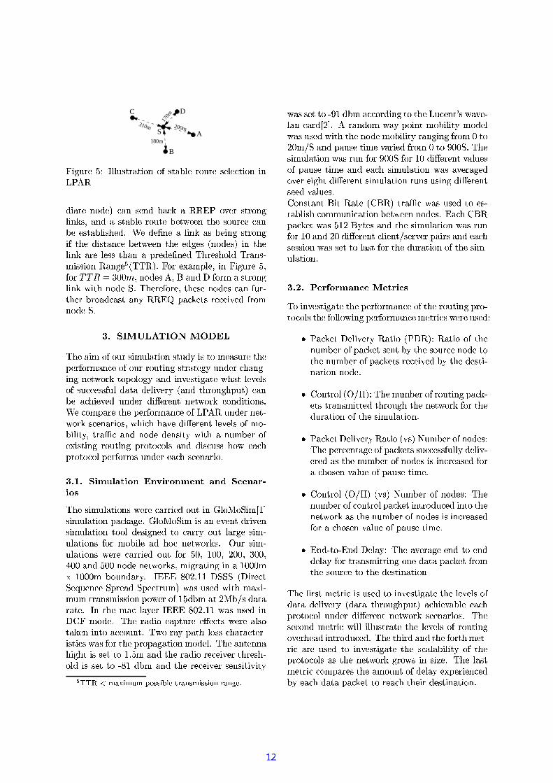
çM·LÉIÒ½f¼" häeÅLÅÒK¸¿Á¾½Â»>Áf·Æ(À!Æ Û ¸¿Áf»IÇÅL¼¥½fÆIÒÁ¾¼-¸¿¼BżÓÁf·Æ(À·LÀÖdÈT×lÚ

ÑZ·¹»>Áf¼ÀÆZÑZ¼Ð-ÓB»#À¸¿¼BÀKÑ ÇK»IÓÂÞs»ÚÝÚÝôÜÈÆ>Ù(¼¡½-¸Áf½¾Æ(ÀÉÅL·ÀKÞ£¸BÕd»IÀKÑ»¸Á»#ÇÅL¼½¾Æ(ÒZÁ¾¼-ÇD¼ÔÁÃ㼡¼BÀÁ¾¶¼¸¾ÆIÒ½ÂÓÔ¼-ÓB»#ÀÇD¼-¼B¸¿Áf»IÇÅ·¹¸¾¶¼BÑTß !¼Ñ¼Ô÷KÀ¼ª»Å·LÀÞ!»(¸hÇD¼¡·LÀɸÁf½¾Æ(ÀÉ· Û Á¾¶¼ÑZ·¹¸Á»#ÀKÓ¡¼Çz¼¡ÁÃϼB¼¡ÀÁf¶¼¯¼ÑZÉI¼¸¯ÎÀÆZÑZ¼B¸ÂÐh·LÀÁf¶¼ÅL·ÀKÞ»I½¾¼ÅL¼B¸f¸hÁf¶K»#Às»º½f¼BÑZ¼¡÷KÀ¼Bѵ¶K½¾¼¸¿¶Æ(ÅLѵd½Â»#ÀK¸¿ÌÍ·¹¸¾¸¾·Æ(ÀÚÝ»IÀÉI¼#娵¨ÚlÐÔßTçÆI½¼Ôá»IÍ¥ºKż(ÕD·LÀçM·LÉIÒ½f¼ ÕÛ Æ(½ à #4#Õ>ÀÆZÑZ¼¸M×1Õ »#ÀzÑ1ý Û ÆI½fÍ »¸Áf½¾Æ(ÀÉÅL·ÀKުè·Á¾¶ÀKƣѼ¥ÊrßDµ¶¼¡½f¼ Û Æ(½¾¼(ÕÁ¾¶K¼B¸¾¼1ÀÆZÑZ¼¸lÓ¡»IÀ Û Ò½¾ÌÁf¶¼¡½hǽfÆ(»(ÑÓ¡»(¸Á³»IÀË!ÚÝÚÝô ú ºK»(ÓÂÞI¼ÔÁ¸½¾¼ÓÔ¼¡·LÙI¼Ñ Û ½fÆIÍÀÆZÑZ¼³Êrß

@ë ° ì ð ­± ì î í î-ï µ¶¼Ý»I·ÍÆ Û ÆIÒK½Ü¸¿·LÍ1ÒKÅL»#Á¾·LÆIÀ-¸ÁfÒKÑZË¥·L¸Á¾Æ³Í¼B»(¸¿ÒK½¾¼Áf¶¼ºD¼¡½ Û ÆI½fÍ-»#ÀKÓ¡¼lÆ Û ÆIÒ½½fÆIÒZÁf·ÀÉ¥¸Áf½f»#Á¾¼BÉIËÒÀKÑZ¼B½¨Ó¶K»#ÀÉIÌ·LÀÉÀ¼ÔÁÃãÆI½fÞÁ¾ÆIºDÆIÅLÆIÉ(Ë»#ÀKÑ·À£ÙI¼¸Áf·É»>Áf¼1è¶K»#Á`ÅL¼¡Ù(¼¡Å¹¸Æ Û ¸¾ÒKÓ¡Ó¡¼B¸f¸ Û ÒKÅÜÑ»>Á»ÑZ¼¡ÅL·Ù(¼¡½fËsÎn»#ÀKÑ!Á¾¶K½¾Æ(ÒÉI¶ºKÒZÁÂÐ`ÓB»#ÀÇD¼»IÓ¶·L¼¡Ù(¼BÑFÒÀKÑZ¼B½ÑZ·öD¼B½¾¼BÀ(ÁÀK¼ÔÁÃãÆI½fÞÓÔÆIÀzÑZ·Áf·Æ(ÀK¸Bß¼lÓÔÆ(ͺK»#½f¼Á¾¶¼Øºz¼B½ Û Æ(½¾Í-»IÀKÓÔ¼¨Æ Û ÖdÈT×lÚÒÀzÑZ¼¡½ÏÀ¼ÔÁ¾ÌÃãÆI½fÞ¯¸fÓÔ¼¡Àz»#½f·Æ¸¡Õ£Ã¨¶·¹Ó¶¶K»ÙI¼hÑZ·ör¼¡½f¼¡ÀÁÝżBÙI¼BÅL¸¨Æ Û ÍÆIÌÇ·LÅL·ÁË(ÕÁ¾½Â»>ûÓ-»IÀKÑÀÆZÑZ¼ÑZ¼¡Àz¸¿·ÁËè·Á¾¶»À£ÒÍaÇz¼B½³Æ Û¼¡á£·¹¸¿Á¾·LÀɽ¾Æ(ÒZÁ¾·LÀɺ½fÆ#ÁfÆZÓÔÆIŹ¸-»#ÀzÑÑZ·L¸fÓÔÒz¸¾¸-¶KÆ>à ¼»IÓ¶º½fÆ#ÁfÆZÓÔÆIÅrºD¼¡½ Û ÆI½fÍ-¸ÒÀKÑZ¼B½¨¼B»IÓ¶¸fÓÔ¼¡Àz»#½f·Æzß

@ëêDë °+039& )+9/.8 J8N, + 7b/.8 $58N) &8FÍ °(4$58B& 7 +9/.2

µ¶¼h¸¾·ÍaÒŹ»>Á¾·LÆIÀz¸ÃϼB½¾¼hÓ¡»I½¾½f·L¼BѪÆIÒZÁ¨·LÀÄÅLÆ(òÆÊ£·LÍÿ¸¾·ÍaÒŹ»>Á¾·LÆIÀ¯ºK»IÓÂÞ>»#É(¼IßÄÅÆòÆÊZ·Í ·¹¸»#À¯¼BÙI¼BÀ(Á¨ÑZ½f·Ù(¼¡À¸¾·ÍaÒŹ»>Á¾·LÆIÀ'Á¾Æ£ÆIÅÝѼB¸¾·É(À¼BÑÁ¾ÆÓ¡»I½¾½fËÆIÒZÁ-Ź»#½fÉI¼¸¿·LÍ¥ÌÒŹ»>Áf·Æ(ÀK¸ Û Æ(½ªÍÆ(Ç·ÅL¼!»(ѶÆZÓÀ¼¡ÁÃÏÆ(½¾ÞZ¸BßæØÒ½¸¿·LÍ¥ÌÒŹ»>Áf·Æ(ÀK¸Ã㼡½f¼Ó¡»I½¾½f·L¼BÑÆIÒÁ Û ÆI½ *#KÕ 3#4#KÕ *#4#KÕ¨à4#4#KÕ'#4#h»#ÀzÑ"*#4#³ÀÆZÑZ¼ÝÀ¼¡ÁÃÏÆ(½¾ÞZ¸BÕIÍ·É(½f»#Á¾·LÀÉh·LÀ¯»3#4#4#IÍá #4# ##Í ÇDÆIÒKÀKÑ»#½fËIßXäôÜôÏô4# ß ýÊÊKÊñÎýØ·½f¼BÓÔÁÊ£¼3Ò¼¡ÀKÓ¡¼1Ê£º½f¼B»(ÑÊ£ºz¼ÓÁf½¾ÒÍÐÝÃã»(¸¨ÒK¸¾¼BÑè·Á¾¶Í-»>áZ·ÌÍaÒÍ*Áf½f»IÀK¸¿Í·¹¸¾¸¾·LÆIÀ1ºDÆ>Ã㼡½Æ Û 3IÑZÇÍ<»#Á #òÇN>¸vÑ»>Á»½Â»>Áf¼I߯äeÀÁf¶¼Í-»IÓŹ»ËI¼B½häôÜôÜô # Zß Ã»I¸`ÒK¸¾¼BÑ·LÀý ãçXÍ¥ÆZÑZ¼(ßµ¶K¼ª½Â»IÑZ·LÆÓB»#ºZÁfÒ½¾¼¯¼Ôör¼BÓÁ¸¥ÃϼB½¾¼¯»IÅL¸¾ÆÁ»#ÞI¼BÀ·ÀÁfƯ»IÓBÓÔÆIÒKÀ(ÁßlµÃãÆ#Ì¢½f»Ëºz»>Á¾¶ÅƸ¾¸ØÓ¶K»#½Â»IÓÔÁ¾¼¡½¾Ì·¹¸Áf·LÓB¸@ûI¸ Û ÆI½MÁf¶¼ÏºK½¾Æ(ºK»#É»>Á¾·LÆIÀhÍÆZÑZ¼BÅnßvµ¶¼»#ÀÁ¾¼BÀÀK»¶·LÉI¶Á·L¸¸¾¼ÔÁãÁ¾Æ Iß>Í »#ÀzÑ-Á¾¶K¼½Â»IÑ·Æa½¾¼ÓÔ¼¡·LÙI¼B½RÁf¶½¾¼¸¿¶ÌÆ(ÅLÑ·L¸h¸¾¼ÔÁ`Á¾ÆªÌS ÑZÇÍ »IÀKÑÁf¶¼½¾¼ÓÔ¼B·Ù(¼¡½`¸¿¼BÀK¸¿·Á¾·LÙ£·ÁË G U ZJIGUK93U C*Ic9cGWPABM[;aZLE3cUVGcc9GIE!;aZLEHAN

ûI¸¸¾¼ÔÁÁfƨÌS RÑZÇÍ9»(Ó¡ÓÔÆ(½fÑ·ÀÉãÁfÆÝÁ¾¶K¼ÜÖÒKÓ¡¼¡ÀÁBé ¸Ã»ÙI¼¡ÌŹ»#ÀÓB»#½ÂÑÿ ^ß³×<½f»IÀKÑZÆ(Í Ã»ËÌ^ºDÆI·LÀÁlÍÆIÇ·LÅL·ÁËÍÆZÑZ¼¡ÅûI¸dÒK¸¿¼Ñ1è·Á¾¶aÁ¾¶K¼ãÀKƣѼãÍÆ(Ç·ÅL·Á˳½f»IÀÉI·LÀÉ Û ½¾Æ(Í #ÝÁfÆ*#IÍ #Ê¥»#ÀKѺz»#ÒK¸¾¼Á¾·LͼlÙ>»#½f·¼Ñ Û ½¾Æ(Í #ÁfÆ 4# #(ÊrßIµ¶K¼¸¾·ÍaÒÅL»#Á¾·LÆIÀûI¸½fÒÀ Û ÆI½ #4#Ê Û Æ(½ #hÑ·ör¼¡½f¼¡ÀÁÜÙ>»#ÅLÒ¼¸Æ Û ºz»#ÒK¸¾¼-Á¾·Lͼ»IÀKѼ»IÓ¶¸¾·ÍaÒÅL»#Á¾·LÆIÀûI¸a»ÙI¼B½f»IÉI¼BÑÆ>ÙI¼B½¼¡·LÉI¶ÁÏÑZ·ör¼¡½f¼¡ÀÁϸ¾·ÍaÒÅL»#Á¾·LÆIÀ½fÒÀK¸ÒK¸¾·LÀÉ1ÑZ·öD¼B½¾¼BÀÁ¸¾¼¡¼BѪÙ>»#ÅLÒ¼B¸BßÏÆIÀz¸Á»#ÀÁ ã·Á1ÚÝ»>Áf¼Î ÚlÐØÁ¾½Â»>ûÓ¥Ãã»(¸ÒK¸¿¼ÑÁfƼB¸¿ÌÁf»IÇÅL·L¸¾¶aÓ¡ÆIÍÍ1ÒÀK·LÓB»>Á¾·LÆIÀ1Çz¼¡ÁÃϼB¼¡À1ÀKƣѼB¸BßdôÜ»(Ó¶ ÚºK»(ÓÂÞI¼ÔÁûI¸V ãËÁ¾¼¸¨»#ÀKѪÁ¾¶K¼`¸¾·LÍ1ÒŹ»>Áf·Æ(ÀªÃ»I¸ã½fÒÀÛ ÆI½ 3#Ø»IÀKÑ 4#ØÑ·ör¼¡½f¼¡ÀÁRÓÔÅL·¼BÀÁ>¸¾¼¡½fÙI¼B½dºz»#·L½f¸v»#ÀzÑ1¼»IÓ¶¸¾¼B¸f¸¿·LÆIÀ-ûI¸Ï¸¿¼¡ÁÜÁ¾Æ¥Å¹»I¸¿Á Û ÆI½ÜÁ¾¶¼`ÑZҽ»>Áf·Æ(ÀÆ Û Áf¶¼Ø¸¾·LÍaÌÒŹ»>Áf·Æ(Àß

@ë ë $ 7a/.7 &<81( $ $') 7b+9(42

µdÆ·LÀ£ÙI¼¸Áf·É»>Á¾¼ÏÁ¾¶K¼¨ºz¼B½ Û Æ(½¾Í-»#ÀzÓÔ¼Æ Û Á¾¶¼¨½fÆIÒZÁf·ÀKɺK½¾ÆIÌÁ¾ÆZÓ¡ÆIŹ¸rÁ¾¶¼ Û Æ(ÅÅLÆ>è·LÀɨºz¼B½ Û Æ(½¾Í-»IÀKÓÔ¼vͼÔÁf½¾·¹Ó¡¸TÃ㼡½f¼vÒK¸¾¼BÑ

È»(ÓÂÞI¼¡Á`ýؼ¡ÅL·Ù(¼¡½fËÚÝ»#Á¾·LÆÎnÈÜýÚlÐ dÚÝ»>Áf·ÆÆ Û Á¾¶K¼À£ÒÍaÇz¼B½ÜÆ Û ºz»IÓÂÞI¼¡ÁR¸¿¼BÀ(ÁÏÇËaÁ¾¶K¼l¸¿Æ(Ò½ÂÓÔ¼ÀÆZÑZ¼¨ÁfÆÁf¶¼lÀ£ÒÍaÇz¼B½ÏÆ Û ºK»IÓÂÞ(¼ÔÁf¸Ü½¾¼ÓÔ¼B·Ù(¼BѥǣË1Áf¶¼ØÑZ¼¸Áf·ÌÀz»>Á¾·LÆIÀÀÆZÑZ¼(ß

ÏÆ(ÀÁ¾½fÆIÅK΢æ[>ùØÐ µ¶K¼RÀ£ÒÍ1ÇD¼¡½dÆ Û ½¾Æ(ÒZÁ¾·LÀɨºK»(ÓÂÞ̼¡Áf¸ÏÁ¾½Â»#Àz¸¿Í·Á¿Á¾¼Ñ-Áf¶½¾Æ(ÒÉI¶¯Á¾¶¼À¼¡ÁÃÏÆ(½¾Þ Û ÆI½ãÁ¾¶K¼ÑÒ½f»#Á¾·LÆIÀÆ Û Á¾¶¼³¸¾·LÍ1ÒŹ»>Áf·Æ(Àß

È»(ÓÂÞI¼¡Á@ýl¼BÅ·LÙI¼B½¾ËÚÝ»>Áf·Æ1ÎÙZ¸fÐ@óÝÒÍaÇz¼B½@Æ Û ÀÆZÑZ¼¸µ¶K¼ãºD¼¡½ÂÓÔ¼BÀÁf»#É(¼ÜÆ Û ºK»IÓÂÞ(¼ÔÁ¸d¸¾ÒKÓ¡Ó¡¼B¸f¸ Û ÒKÅÅL˳ÑZ¼¡ÅL·LÙ(̼B½¾¼Ñ¯»(¸ÜÁf¶¼ÀÒKÍ1ÇD¼¡½Æ Û ÀKƣѼB¸ã·L¸·LÀKÓ¡½¾¼»I¸¾¼BÑ Û Æ(½»-Ó¶KÆ(¸¾¼¡À¯Ù>»IÅÒ¼hÆ Û ºK»IÒK¸¾¼ØÁf·Í¼(ß

ÏÆ(ÀÁ¾½fÆIŨÎ^æ[#ùØХΠÙZ¸ÂÐ`óÝÒÍaÇz¼B½hÆ Û ÀKƣѼB¸ `µ¶K¼À£ÒÍaÇz¼B½dÆ Û ÓÔÆIÀÁf½¾Æ(ÅIºK»(ÓÂÞI¼ÔÁ·LÀÁ¾½fÆZÑZÒKÓÔ¼Ñ`·ÀÁfÆÝÁ¾¶K¼ÀK¼ÔÁÃãÆI½fÞ¥»(¸Á¾¶K¼lÀ£ÒÍ1ÇD¼¡½ÏÆ Û ÀÆZÑZ¼¸Ü·¹¸R·LÀKÓ¡½¾¼»I¸¾¼BÑÛ Æ(½Ý»-Ó¶Æ(¸¾¼¡ÀªÙ>»#ÅLÒ¼hÆ Û ºK»#ÒK¸¾¼Á¾·LͼIß

ôÜÀKÑ£Ì^Á¾ÆIÌ¢ôÜÀKÑýl¼BÅL»Ë µ¶¼1»ÙI¼B½f»IÉI¼¼¡ÀKÑÁ¾Æ¼BÀKÑѼ¡Å¹»Ë Û ÆI½ãÁ¾½Â»#ÀK¸¾Í·Á¾Á¾·LÀÉ¥ÆIÀ¼`Ñ»>Á»1ºz»IÓÂÞI¼¡Á Û ½fÆIÍÁf¶¼³¸¾ÆIÒ½ÂÓÔ¼Á¾Æ¥Áf¶¼³ÑZ¼B¸¿Á¾·LÀK»#Á¾·LÆIÀ

µ¶¼l÷K½f¸¿ÁÜͼÔÁf½¾·¹ÓÝ·¹¸ÏÒK¸¿¼ÑÁ¾Æ1·À£ÙI¼¸Áf·É»>Áf¼¨Á¾¶¼ØżBÙI¼BÅL¸ÜÆ ÛÑ»#Áf»ÑZ¼¡ÅL·Ù(¼¡½fËÎÑ»#Áf»!Á¾¶K½¾Æ(ÒÉI¶ºKÒZÁÂÐ¥»IÓ¶K·¼BÙ»IÇÅL¼ª¼»IÓ¶º½fÆ#ÁfÆ£Ó¡ÆIÅãÒÀKÑZ¼B½ÑZ·öD¼B½¾¼BÀ(Á-À¼¡ÁÃÏÆ(½¾Þ¸fÓÔ¼BÀK»#½f·Æ¸¡ßµ¶K¼¸¾¼BÓÔÆ(ÀKÑ!Í¥¼¡Á¾½f·LÓè·LÅLÅR·ÅLÅLÒK¸Áf½f»#Á¾¼Áf¶¼ÅL¼¡ÙI¼BÅL¸`Æ Û ½fÆIÒÁ¾·LÀÉÆ>ÙI¼B½¾¶K¼B»IÑØ·LÀ(Áf½¾ÆZÑZÒzÓÔ¼BÑß@µ¶¼Áf¶·½ÂÑh»#ÀzÑÁ¾¶¼ Û Æ(½¿Áf¶hͼÔÁ¿Ì½f·LÓ»I½¾¼ÒK¸¾¼BÑ ÁfÆ·À£ÙI¼¸Áf·É»>Áf¼ªÁf¶¼¸fÓ¡»IÅL»IÇ·ÅL·ÁËÆ Û Á¾¶K¼º½fÆ#ÁfÆ£Ó¡ÆIŹ¸h»I¸Áf¶¼À¼¡ÁÃÏÆ(½¾ÞÉ(½¾Æ>Ãݸ`·LÀ¸¿·L衼(߯µ¶¼-Ź»I¸¿ÁͼÔÁf½¾·¹ÓØÓ¡ÆIͺK»I½¾¼¸Á¾¶K¼`»IÍÆIÒÀÁÏÆ Û ÑZ¼BÅL»Ë-¼¡á£ºD¼¡½f·L¼¡ÀKÓ¡¼BÑǣ˼B»(Ó¶ÑK»>Áf»¥ºK»(ÓÂÞI¼¡ÁãÁfƽ¾¼»IÓ¶Áf¶¼¡·L½lÑZ¼¸Áf·Àz»>Á¾·LÆIÀ@ß

/@ë ² h°ð ±a°

µ¶·¹¸¸¾¼BÓÔÁ¾·LÆIÀK¸ÉI·LÙI¼B¸»ÑZ·L¸fÓÔÒz¸¾¸¾·Æ(À9ÆIÀXÁ¾¶K¼s¸¾·ÍaÒÅL»#ÌÁf·Æ(ÀF½f¼B¸¾ÒÅÁ¸Ãϼ!ÆIÇZÁ»#·LÀ¼BÑ Û ÆI½ÆIÒ½½fÆIÒZÁf·Àɸ¿Á¾½Â»>Á¾¼¡ÌÉ(·¼¸¡ß,µ@Æ·LÀ£ÙI¼B¸¿Á¾·LÉ(»#Á¾¼Á¾¶K¼ºz¼B½ Û Æ(½¾Í-»IÀKÓÔ¼Æ Û ÖdÈT×lÚè·Á¾¶»#ÀKÑ!è·Á¾¶Æ(ÒZÁ1¸Á»#ÇÅL¼Å·LÀÞ¸¿Á¾½Â»>Áf¼¡É(ËÎ ·LÀ¸¾¼BÓÔÁ¾·LÆIÀß £ÐÕ>Ãã¼Ï½Â»#À1ÁÃÏÆ`ÑZ·öD¼B½¾¼BÀ(ÁÙ(¼¡½Â¸¿·LÆIÀK¸dÆ Û Ö@ÈT×ØÚhß>µ¶¼B¸¾¼»I½¾¼dÖ@ÈT×ØÚhÕIè¶K·LÓ¶¯Ó¡ÆIÀK¸¾·¹¸ÁÂ¸Æ Û ¸¾¼BÓÔÁ¾·LÆIÀK¸ Zß `»#ÀKÑ ß àKÕÖdÈT×lÚÌÊ趷¹Ó¶ª¸¾¼BÓÔÁ¾·LÆIÀK¸ Zß ZÕ Zß à1»IÀKÑ ß zßMµ¶¼ºD¼¡½¾ÌÛ Æ(½¾Í-»#ÀzÓÔ¼¨Æ Û Æ(Ò½ÜÖdÈT×lÚ¸¿Á¾½Â»>Áf¼¡ÉI·L¼B¸R趼¡½f¼lÓÔÆ(ͺK»#½f¼BÑè·Á¾¶Ö@×ØÚ h»#ÀKÑ×læý¨þaß

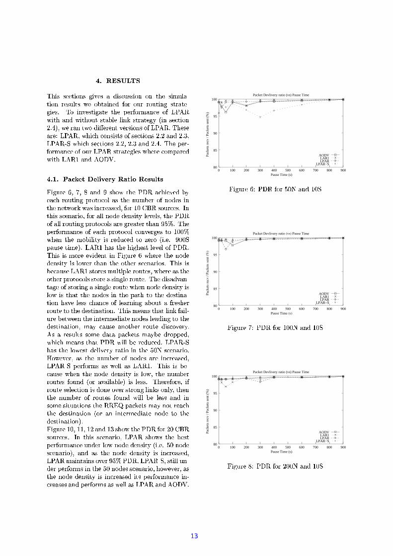
/dëêDë &<(.$')ªï$3-+ ,6$'7 ² & )3+-/² $52303-)2çM·LÉIÒ½f¼" Õ £Õ »IÀKÑ]¸¾¶Æ>à Áf¶¼ªÈÏýØÚ »(Ó¶·L¼¡ÙI¼ÑÇ˼»IÓ¶½¾Æ(ÒZÁ¾·LÀɺ½fÆ#ÁfÆ£Ó¡ÆIÅÜ»(¸Á¾¶¼¯ÀÒKÍ1ÇD¼¡½1Æ Û ÀKƣѼB¸³·LÀÁf¶¼ÏÀK¼ÔÁÃãÆI½fÞØûI¸d·ÀzÓÔ½f¼B»I¸¾¼BÑÕ Û Æ(½ # Ús¸¿Æ(Ò½fÓ¡¼B¸BßäeÀÁf¶·L¸¨¸fÓÔ¼BÀK»#½f·LÆKÕ Û ÆI½¨»#ÅLÅrÀÆZÑZ¼hÑZ¼¡ÀK¸¾·ÁËżBÙI¼BÅL¸BÕÁ¾¶¼hÈÜýÚÆ Û »IÅÅZ½fÆIÒZÁf·ÀKÉhº½¾ÆIÁ¾ÆZÓÔÆ(ÅL¸v»I½¾¼¨É(½¾¼»>Á¾¼B½MÁ¾¶K»IÀ'¯ßvµ¶¼ºD¼¡½ Û ÆI½fÍ-»#ÀKÓ¡¼Æ Û ¼»IÓ¶º½fÆ#ÁfÆ£Ó¡ÆIÅãÓÔÆIÀ£Ù(¼¡½fÉI¼B¸hÁ¾Æ 3#4#趼BÀ'Áf¶¼ÍÆIÇ·LÅ·ÁË·¹¸¥½¾¼ÑZÒKÓÔ¼ÑÁfÆ!èB¼¡½fÆ Î·nß ¼Iß 4# #(ʺK»IÒK¸¾¼ØÁf·Í¼ÐßÜÖd×lÚ `¶K»(¸ãÁ¾¶¼h¶·LÉI¶K¼B¸¿ÁÝżBÙI¼¡ÅTÆ Û ÈÏýØڳߵ¶·¹¸`·¹¸ØÍÆ(½¾¼¼¡Ù£·¹ÑZ¼¡ÀÁh·LÀçM·LÉIÒ½f¼ 趼B½¾¼aÁ¾¶K¼-ÀÆZÑZ¼ÑZ¼BÀK¸¾·ÁË·¹¸lÅLÆ>ÃϼB½¨Á¾¶z»#ÀÁf¶¼aÆIÁ¾¶¼B½Ø¸fÓÔ¼BÀK»#½f·Æ¸¡ßص¶·L¸Ø·¹¸ÇD¼BÓB»#ÒK¸¾¼ÏÖd×lÚ ã¸ÁfÆI½f¼B¸ÍaÒÅÁ¾·LºÅ¼ã½fÆIÒZÁf¼B¸BÕ>趼¡½f¼Ï»(¸Áf¶¼ÆIÁ¾¶¼B½@º½fÆ#ÁfÆ£Ó¡ÆIŹ¸@¸¿Á¾Æ(½¾¼Ü»l¸¿·LÀÉIÅL¼Ü½fÆIÒÁ¾¼IßMµ¶¼ÏÑ·L¸f»IÑZÙ>»IÀZÌÁ»#ÉI¼¨Æ Û ¸ÁfÆI½f·ÀÉh»³¸¾·LÀÉIÅL¼¨½¾Æ(ÒZÁ¾¼¨Ã¨¶K¼¡À-ÀÆZÑZ¼lѼ¡ÀK¸¾·ÁË¥·¹¸ÅLÆ>Ã*·¹¸lÁf¶K»>Á`Áf¶¼ÀÆZÑZ¼B¸`·LÀÁf¶¼ºK»>Áf¶ÁfƯÁf¶¼-ÑZ¼B¸¿Á¾·LÀK»#ÌÁf·Æ(À¶z»ÙI¼Å¼¸¾¸aÓ¶K»#ÀzÓÔ¼Æ Û ÅL¼B»#½fÀ·LÀÉ»#ÇDÆIÒZÁ¥» Û ½¾¼¸¿¶¼B½½fÆIÒZÁf¼Á¾ÆlÁ¾¶¼ãÑZ¼B¸¿Á¾·LÀK»#Á¾·LÆIÀßMµ¶·L¸dͼB»IÀK¸Áf¶K»>ÁMÅ·LÀÞ Û »#·LÅÌÒ½f¼¨ÇD¼ÔÁÃ㼡¼¡À¥Áf¶¼Ý·LÀ(Áf¼¡½fͼBÑZ·¹»>Áf¼ãÀKƣѼB¸RÅL¼B»(ÑZ·LÀÉÁ¾ÆhÁf¶¼ÑZ¼¸Áf·Àz»>Á¾·LÆIÀ@ÕlÍ-»ËÓ¡»#Òz¸¿¼»#ÀÆIÁ¾¶¼B½ª½fÆIÒZÁf¼Ñ·L¸fÓÔÆ>Ù(¼¡½fËIß×ظ¥»!½f¼B¸¾ÒÅÁ¸¸¿Æ(Í¥¼Ñ»#Áf»ºK»IÓÂÞ(¼ÔÁ¸1Í-»Ë£Çz¼ÑZ½fÆIººD¼BÑÕ趷¹Ó¶ͼB»#Àz¸ãÁ¾¶K»#ÁØÈÜýÚXè·ÅLÅÇD¼³½¾¼ÑZÒKÓ¡¼BÑTßÜÖdÈT×lÚÌʶK»(¸¨Áf¶¼1ÅLÆ>Ãϼ¸ÁÑZ¼¡ÅL·Ù(¼¡½f˯½Â»>Áf·Æ·LÀÁf¶¼ 4#Ió*¸fÓÔ¼BÀK»#½f·ÆzßùlÆ>ÃϼBÙI¼¡½ÕR»I¸aÁf¶¼À£ÒÍ1ÇD¼¡½Æ Û ÀÆZÑZ¼B¸-»I½¾¼·LÀKÓÔ½f¼B»(¸¿¼ÑTÕÖdÈT×lÚÌʺD¼¡½ Û ÆI½fÍ-¸a»(¸aÃ㼡ÅLŨ»I¸¥Ö@×ØÚ Iß'µ¶K·L¸·¹¸¥Çz¼¡ÌÓB»#ÒK¸¾¼-趼¡ÀÁf¶¼ÀÆZÑZ¼ªÑZ¼¡ÀK¸¾·ÁË!·¹¸³ÅLÆ>ÃhÕ@Áf¶¼À£ÒÍaÇz¼B½½fÆIÒZÁf¼B¸ Û ÆIÒKÀKÑÎÆI½»Ù>»#·LŹ»#ÇÅL¼Ð1·L¸ÅL¼B¸f¸Bß µ¶¼B½¾¼ Û ÆI½f¼IÕR· Û½fÆIÒZÁf¼Ý¸¿¼BżÓÁf·Æ(À¥·¹¸ÜÑÆIÀ¼ÝÆ>Ù(¼¡½R¸¿Á¾½fÆIÀÉ`ÅL·ÀKÞ£¸ÜÆIÀÅLËIÕIÁ¾¶¼BÀÁf¶¼!À£ÒÍaÇz¼B½ªÆ Û ½fÆIÒZÁf¼B¸ Û ÆIÒÀKÑFè·ÅLÅ`Çz¼ÅL¼B¸f¸ª»IÀKÑ·LÀ¸¾ÆIͼl¸¾·ÁfÒK»>Áf·Æ(ÀK¸Áf¶¼`ÚÝÚÝô ú ºK»(ÓÂÞI¼¡Áf¸RÍ-»Ë¥ÀÆ#Áã½¾¼»IÓ¶Áf¶¼ÑZ¼B¸¿Á¾·LÀK»#Á¾·LÆIÀ9Î Æ(½¯»#À ·ÀÁf¼¡½fÍ¥¼ÑZ·¹»>Á¾¼ÀKƣѼÁ¾ÆÁf¶¼ÑZ¼¸Áf·Àz»>Á¾·LÆIÀDÐßçM·LÉIÒ½f¼ #KÕ IÕ »#ÀKÑ à¨¸¿¶KÆ>ÃÁf¶¼ÏÈÏýØÚ Û Æ(½ *# Ú¸¾ÆIÒ½ÂÓÔ¼¸¡ßäeÀsÁ¾¶K·L¸-¸fÓÔ¼BÀK»#½f·ÆzÕRÖ@ÈT×ØÚ ¸¾¶Æ>Ãݸ1Á¾¶¼ÇD¼B¸¿ÁºD¼¡½ Û ÆI½fÍ-»#ÀKÓ¡¼ÝÒÀKÑZ¼B½ÅÆ>ÃÀÆZÑZ¼`ÑZ¼BÀK¸¿·ÁËÎ ·^ß ¼(ß *#1ÀÆZÑZ¼¸fÓÔ¼BÀK»#½f·Æ£ÐÕ¨»#ÀzÑ»I¸Á¾¶¼!ÀÆZÑZ¼!ÑZ¼BÀK¸¾·ÁË ·L¸ª·LÀKÓÔ½f¼B»(¸¿¼ÑTÕÖdÈT×lÚÍ-»#·LÀÁf»#·LÀK¸TÆ>Ù(¼¡½'ÈÜýÚhßBÖdÈT×lÚÌÊrÕB¸¿Á¾·LÅLÅ(ÒÀÌÑZ¼B½ºz¼B½ Û Æ(½¾Í-¸v·LÀ¥Á¾¶¼>4#ØÀKƣѼB¸R¸fÓÔ¼BÀK»#½f·ÆzÕ>¶Æ>Ã㼡ÙI¼B½BÕ#»(¸Áf¶¼ÀÆZÑZ¼ÑZ¼¡Àz¸¿·ÁË·¹¸`·ÀKÓ¡½¾¼»I¸¾¼BÑ·Á¸hºz¼B½ Û Æ(½¾Í-»IÀKÓÔ¼¥·ÀÌÓ¡½¾¼»I¸¾¼B¸@»IÀKÑaºz¼B½ Û Æ(½¾Í-¸v»I¸MÃ㼡ÅLÅ£»(¸vÖ@ÈT×lÚs»#ÀKÑ¥×læý¨þaß

80

85

90

95

100

0 100 200 300 400 500 600 700 800 900

Pack

ets

recv

/ Pa

cket

s se

nt (

%)

Pause Time (s)

Packet Devlivery ratio (vs) Pause Time

AODVLAR1LPAR

LPAR−S

çM·LÉIÒ½f¼[ RÈÜýÚ Û ÆI½>*#(óñ»#ÀKÑ #Ê

80

85

90

95

100

0 100 200 300 400 500 600 700 800 900

Pack

ets

recv

/ Pa

cket

s se

nt (%

)

Pause Time (s)

Packet Devlivery ratio (vs) Pause Time

AODVLAR1LPAR

LPAR−S

çM·É(Ò½f¼= RÈÜýÚ Û Æ(½ # #IóX»#ÀKÑ #Ê

80

85

90

95

100

0 100 200 300 400 500 600 700 800 900

Pack

ets

recv

/ Pa

cket

s se

nt (

%)

Pause Time (s)

Packet Devlivery ratio (vs) Pause Time

AODVLAR1LPAR

LPAR−S

çM·É(Ò½f¼ RÈÜýÚ Û Æ(½ *# #IóX»#ÀKÑ #Ê

80

85

90

95

100

0 100 200 300 400 500 600 700 800 900

Pack

ets

recv

/ Pa

cket

s se

nt (

%)

Pause Time (s)

Packet Devlivery ratio (vs) Pause Time

AODVLAR1LPAR

LPAR−S

çM·LÉIÒ½f¼[RÈÜýÚ Û ÆI½Ýà4# #Ióñ»#ÀzÑ 3#(Ê

80

85

90

95

100

0 100 200 300 400 500 600 700 800 900

Pack

ets

recv

/ Pa

cket

s se

nt (

%)

Pause Time (s)

Packet Devlivery ratio (vs) Pause Time

AODVLAR1LPAR

LPAR−S

çM·É(Ò½f¼ 3#ÈÜýÚ Û Æ(½>*#Ióñ»IÀKÑ 4#(Ê

çKÒ½¿Áf¶¼¡½fÍÆI½f¼IÕØ·ÀÁ¾¶¼¶·LÉI¶ÀÆZÑZ¼ÑZ¼¡Àz¸¿·ÁËF¸fÓÔ¼¡Àz»#½f·Æηnß ¼Iß BàзÁÇz¼BÉI·LÀK¸MÁ¾ÆÆIÒZÁºD¼¡½ Û ÆI½fÍñÁ¾¶¼¨ÆIÁ¾¶¼B½v½¾Æ(ÒZÁ¾·LÀɺ½fÆ#ÁfÆZÓÔÆIŹ¸Bß㵶·¹¸Ý·LÀKÓ¡½¾¼»I¸¾¼h·ÀºD¼¡½ Û ÆI½fÍ-»#ÀKÓ¡¼³·L¸ØÑZÒ¼hÁfÆÁf¶¼¯»Ù>»#·LÅL»IÇ·LÅ·ÁËÆ Û ÍÆI½f¼¸¿Áf»#ÇKż½fÆIÒÁ¾¼B¸³Ã¨¶¼¡ÀÓ¡ÆI̺ͥK»I½¾¼ÑsÁ¾ÆÁ¾¶K¼ÅL¼B»I¸¿Á¯ÑZ¼BÀK¸¿¼!¸¾Ó¡¼¡ÀK»I½¾·LÆ(¸BßF×læý¨þ »IÅL¸¾ÆºD¼¡½ Û ÆI½fÍ-¸Ã㼡ÅLÅ»(ÓÔ½fÆ(¸f¸¯»#ÅLŽf»IÀÉI¼¸Æ Û ÀKƣѼÑZ¼BÀK¸¾·ÁË(ßùlÆ>ÃϼBÙI¼¡½Õ`·Á¸Á»#½¾ÁÁ¾ÆÒÀzÑZ¼¡½!ºz¼B½ Û Æ(½¾Í Ö@ÈT×lÚ »IÀKÑÖdÈT×lÚÌÊ-·LÀÁf¶¼hà4#4#1ÀÆZÑZ¼À¼ÔÁÃãÆI½fÞ-¸¾Ó¡¼¡ÀK»I½¾·LÆKßvÖ@×ØÚ »(Ó¶·¼BÙI¼¸Á¾¶K¼lÅLÆ>Ãϼ¸ÁãżBÙI¼¡Å¹¸ÏÆ Û ÈÜýÚ·LÀÁf¶·¹¸Ï¸fÓÔ¼BÀK»#½f·Æzßµ¶·¹¸ª·L¸ÍÆI½f¼¼BÙ·¹ÑZ¼BÀ(ÁÒÀKÑZ¼B½Á¾¶¼¶·LÉI¶¼B½ªÍÆIÇK·ÅL·ÁËηnß ¼I߸¿Í-»#ÅLÅL¼¡½lºz»#ÒK¸¾¼hÁ¾·LͼB¸ÂÐÕT趼B½¾¼1Å·LÀÞ Û »#·LÅÒK½¾¼a½f»#Á¾¼·¹¸³¶·LÉI¶K¼¡½ßµ¶¼¡½f¼ Û Æ(½¾¼(Õd·LÀÁ¾¶K·L¸¥¸¾Ó¡¼¡ÀK»I½¾·LÆKÕ@Á¾¶¼ªºzÆ(·ÀÁ¾ÌÁfÆ#Ì¢ºzÆ(·ÀÁܽfÆIÒZÁf·ÀKÉ1º½fÆ#ÁfÆ£Ó¡ÆIŹ¸Üӡż»#½fÅË¥ÆIÒZÁãºz¼B½ Û Æ(½¾ÍÁf¶¼¸¾ÆIÒ½ÂÓÔ¼½fÆIÒZÁf·Àɺ½fÆ#ÁfÆZÓÔÆIÅηnß ¼IßRÖd×lÚ Ðß

/dë ë ´ /68N) 7b/,3Ýî ,.$'71$5&Ͳ%$520 3 )32çM·LÉIÒ½f¼ zÕ3Õ 3 »#ÀKÑ ¸¾¶Æ>Ã,Á¾¶¼sÀ£ÒÍ1ÇD¼¡½Æ ÛÓ¡ÆIÀÁ¾½fÆIÅ`ºK»(ÓÂÞI¼ÔÁ¸·ÀÁf½¾ÆZÑZÒKÓ¡¼BÑX·LÀ(ÁfÆ Á¾¶¼ÀK¼ÔÁÃãÆI½fÞÇ˼»IÓ¶½fÆIÒZÁf·ÀKÉsº½fÆ#ÁfÆZÓÔÆIÅ^Õ Û Æ(½ # Ú,¸¿Æ(Ò½ÂÓÔ¼B¸Bß äeÀ×læý¨þaÕ(ÍÆ(½¾¼ØÆ>ÙI¼¡½f¶¼»IÑ·¹¸Ï·LÀÁ¾½fÆZÑZÒKÓÔ¼Ñ-·LÀ(ÁfÆ1Áf¶¼À¼ÔÁ¾ÌÃãÆI½fÞÁ¾¶K»IÀ1Áf¶¼¨Æ#Áf¶¼¡½v½fÆIÒZÁf·ÀÉ`¸¿Á¾½Â»>Á¾¼BÉI·L¼B¸Bßdµ¶·¹¸v·¹¸vÇz¼¡ÌÓB»#ÒK¸¾¼IÕ£×læý¨þ9ÑZÆ£¼B¸ãÀÆIÁÏÁ»#ÞI¼»#À£Ë-ͼB»(¸¿Ò½f¼¡Í¼BÀ(Á¸RÁfƽf¼BÑZÒzÓÔ¼ÏÁ¾¶¼½fÆIÒZÁf¼Ñ·L¸fÓÔÆ>Ù(¼¡½f˽f¼¡É(·Æ(À³· Û Áf¶¼¨¸¿Æ(Ò½fÓ¡¼ã»IÀKÑ

80

85

90

95

100

0 100 200 300 400 500 600 700 800 900

Pack

ets

recv

/ Pa

cket

s se

nt (

%)

Pause Time (s)

Packet Devlivery ratio (vs) Pause Time

AODVLAR1LPAR

LPAR−S

çM·É(Ò½f¼ ÈÜýÚ Û ÆI½ # #Ióñ»#ÀzÑ 4#(Ê

80

85

90

95

100

0 100 200 300 400 500 600 700 800 900

Pack

ets

recv

/ Pa

cket

s se

nt (

%)

Pause Time (s)

Packet Devlivery ratio (vs) Pause Time

AODVLAR1LPAR

LPAR−S

çM·É(Ò½f¼ ÈÜýÚ Û ÆI½ *# #Ióñ»#ÀzÑ 4#(Ê

80

85

90

95

100

0 100 200 300 400 500 600 700 800 900

Pack

ets

recv

/ Pa

cket

s se

nt (

%)

Pause Time (s)

Packet Devlivery ratio (vs) Pause Time

AODVLAR1LPAR

LPAR−S

çM·É(Ò½f¼ àÈÜýÚ Û ÆI½Ýà4# #Ióñ»#ÀzÑ 4#(Ê

0

2000

4000

6000

8000

10000

12000

14000

16000

18000

0 100 200 300 400 500 600 700 800 900

Con

trol

pac

kets

(pa

cket

s)

Pause Time (s)

Control packets (vs) Pause Time

AODVLAR1LPAR

LPAR−S

çd·LÉIÒK½¾¼ 㵨ÚÝÖºK»IÓÂÞ(¼ÔÁ¸ Û Æ(½>*#(óX»IÀKÑ #Ê

Áf¶¼!ÑZ¼¸Áf·Àz»>Á¾·LÆIÀ¶z»ÙI¼½f¼BÓÔ¼BÀÁ¾ÅLË Ó¡ÆIÍÍ1ÒÀK·LÓB»>Á¾¼Ñ*Î Æ(½Áf¶¼¨¸¿Æ(Ò½fÓ¡¼Ü¶K»(¸vÅÆZÓB»>Á¾·LÆIÀa·À Û ÆI½fÍ»#Á¾·LÆIÀ¥»#ÇDÆIÒZÁvÁ¾¶K¼Ñ¼B¸¿ÌÁf·ÀK»#Á¾·LÆIÀzÐÔߪæØÀÁf¶¼ÓÔÆ(ÀÁ¾½Â»#½fËIÕT·LÀÖd×lÚ ¥ÁÃãÆ Û »IÓÁfÆI½Â¸Ó¡ÆIÀÁ¾½f·ÇKÒZÁ¾¼aÁ¾Æ½¾¼ÑZÒKÓ¡·ÀɽfÆIÒZÁf·ÀÉÆ>ÙI¼B½¾¶K¼B»IÑß³çd·L½Â¸ÁfÅË(ÕÀÆZÑZ¼¸RÓ¡»IÀ¶K»ÙI¼¨ÍaÒÅÁf·ºKżݽfÆIÒÁ¾¼B¸Á¾Æ1ÑZ¼¸Áf·Àz»>Á¾·LÆIÀz¸Ýλ(¸ÑZ·¹¸fÓÔÒK¸f¸¿¼Ñ¼»#½fÅ·L¼¡½ÐÕT趷¹Ó¶Í-»Ë½f¼BÑÒKÓÔ¼aÁ¾¶¼À£ÒÍaÇz¼B½Æ Û ½fÆIÒÁ¾¼ÜÑZ·¹¸fÓÔÆ>ÙI¼B½¾·L¼B¸r·LÀ·Á¾·¹»>Áf¼BÑ Û Æ(½@¼B»(Ó¶h¸¿½ÂÓ3#ÑZ¼B¸¿Á@ºK»I·½Õ趼B½¾¼»I¸·LÀ×læý¨þ1Õz¼B»IÓ¶ÀÆZÑZ¼hÆ(ÀÅL˪¸¿Á¾ÆI½f¼B¸¨»-¸¾·LÀÉIÅL¼½fÆIÒZÁf¼IßvÊ£¼BÓ¡ÆIÀKÑZÅLËIÕ(·ÀÖd×lÚ (ÕI· Û ¸¿Æ(Ò½fÓ¡¼ÀÆZÑZ¼B¸¶z»ÙI¼ÅÆIÌÓB»>Á¾·LÆIÀ1·À Û Æ(½¾Í-»#Á¾·LÆIÀ1»IÇzÆ(ÒZÁ@Áf¶¼Ï½f¼Ò·L½f¼BѳÑZ¼¸Áf·Àz»>Á¾·LÆIÀ@ÕÁf¶¼¡ËFÓB»#ÀXÒK¸¾¼ÚJTÊ În»I¸ÑZ¼¸¾Ó¡½¾·LÇD¼BѼB»#½fÅL·¼B½ÂÐÔÕØ趷¹Ó¶ͷLÀ·Í·¹¸¿¼¸Î ÆI½`ÅLÆZÓ¡»#ÅL·¹¸¿¼¸fШÁ¾¶¼-¸¾¼B»#½ÂÓ¶»I½¾¼»-Á¾Æ»ªºK»#½¾ÌÁf·LÓ¡ÒÅL»I½h½¾¼BÉI·LÆIÀß-µ¶¼»(ÑZÙ>»#ÀÁf»IÉI¼Æ Û Á¾¶·¹¸³·¹¸Á¾¶z»>Á³Áf¶¼À£ÒÍaÇz¼B½lÆ Û ÀÆZÑZ¼¸Ý·LÀ£ÙIÆIÅLÙI¼Ñ·ÀǽfÆ(»(ÑÓ¡»(¸Áf·ÀKÉÚÝÚÝô úºK»(ÓÂÞI¼¡Áf¸Ü»I½¾¼½f¼BÑZÒKÓ¡¼BÑTգ趷¹Ó¶¯Í¼»#ÀK¸ÏÁ¾¶z»>Á Û ¼¡Ã㼡½¨ÓÔÆ(ÀZÌÁf½¾Æ(Å1ºK»(ÓÂÞI¼ÔÁ¸»I½¾¼Áf½f»IÀK¸¾Í¥·Á¿Áf¼BÑTß0µ¶·¹¸!»IÅL¸¾ÆͼB»#Àz¸ÍÆI½f¼ãÇK»#ÀKÑè·LÑ£Áf¶Á¾Æ`ÇD¼Ý»Ù»I·Å¹»#ÇKż Û ÆI½vÁf¶¼¨ÀÆZÑZ¼¸vÁ¾¶K»#Á»I½¾¼ÀÆIÁv·LÀÁ¾¶K¼Ý¸¿¼»#½ÂÓ¶a»#½f¼B»`»IÀKÑ¥½¾¼ÑZÒKÓÔ¼¨Ó¶K»IÀÀ¼BÅKÓÔÆ(ÀZÌÁf¼¡ÀÁ¾·LÆIÀßMÖ@ÈT×ØÚ»#ÀKÑhÖdÈT×lÚÌÊrաè¶K·LÓ¶hÒK¸¾¼Áf¶¼Ïà#Ì¢¸¿Áf»#Á¾¼½fÆIÒZÁf¼-ÑZ·L¸fÓÔÆ>Ù(¼¡½fË»#ÅLÉIÆI½f·Á¾¶ÍÕº½fÆZÑZÒKÓ¡¼¥ÅL¼B¸f¸`Æ>ÙI¼B½¾¶K¼B»IÑÁf¶K»#ÀhÖ@×ØÚ IÕÑZ¼¸¿º·Á¾¼ÜÆIÀÅLËظ¿Á¾Æ(½¾·LÀɨ¸¿·LÀÉ(ż½fÆIÒZÁf¼B¸Bß@µ¶·¹¸·¹¸TÇD¼BÓ¡»IÒK¸¾¼·ÀhÆ(Ò½à>Ìe¸Á»>Áf¼½¾Æ(ÒZÁ¾¼RÑZ·¹¸fÓÔÆ>ÙI¼B½¾ËÝ»IÅÉ(ÆI½f·Áf¶ÍÕ· Û ÒKÀ¼ÔáZº·L½¾¼ÑÅÆZÓB»>Á¾·LÆIÀ·LÀ Û ÆI½fÍ-»>Á¾·LÆIÀ·¹¸Ý»Ù>»#·LÅL»IÇÅL¼IÕZÁf¶¼¸¾ÆIÒ½ÂÓÔ¼¨ÀKƣѼÝè·ÅLÅ÷z½f¸¿ÁÏ»>Á¾Á¾¼BÍ¥ºÁÜÁ¾Æ¥ÑZ·¹¸¾Ó¡Æ>ÙI¼¡½fË1»`½fÆIÒZÁf¼Ç£ËXÒÀ·¹Ó¡»I¸¿Á¾·LÀɽ»>Áf¶¼¡½!·À ǽ¾Æ»IÑÓB»I¸¿Á¾·LÀÉ9λ(¸º½f¼¡Ù£·ÌÆ(ÒK¸¿ÅLË1ÑZ¼¸¾Ó¡½¾·LÇD¼BÑ¥·ÀÁf¶¼lýõlÚÝý»#ÅLÉIÆ(½¾·Á¾¶Í<·À-¸¾¼BÓÔÁ¾·LÆIÀß (Ðßµ¶·L¸¥Í¼B»IÀK¸1Á¾¶K»#Á Û ¼BÃϼB½¥Ó¡ÆIÀÁ¾½fÆIÅϺK»IÓÂÞ(¼ÔÁf¸¥»#½f¼Áf½f»IÀK¸¿Í·Á¿Áf¼BÑ Á¾¶K½¾Æ(ÒÉI¶ Á¾¶K¼À¼ÔÁÃãÆI½fÞrßXÖdÈT×lÚÌÊ Û Ò½¾ÌÁf¶¼¡½h½f¼BÑZÒzÓÔ¼B¸ØÁf¶·L¸³Æ>ÙI¼¡½f¶¼»IÑÇ£Ë KÆ£ÆZÑZ·LÀÉÆ>ÙI¼B½ÅL·LÀÞZ¸Ã¨¶·¹Ó¶¶K»ÙI¼ÓÔ¼B½¿Á»#·LÀ!ÅL¼¡Ù(¼¡ÅÆ Û ¸¿Áf»#ÇK·ÅL·ÁË(ß-µ¶¼»IÑZÙ>»IÀZÌÁ»#ÉI¼-Æ Û Á¾¶·¹¸³·¹¸hÁf¶K»>Á1½fÆIÒÁ¾¼Í-»ËŹ»I¸¿Á1ÅLÆIÀÉ(¼¡½Õ@趷¹Ó¶ͼB»IÀK¸ Û ¼¡Ã㼡½½¾Æ(ÒZÁ¾¼³½f¼BÓB»#ŹÓÔÒŹ»>Áf·Æ(ÀK¸Ýè·LÅLÅMÇD¼¥½¾¼3(ÒK·½f¼BÑ»IÀKÑ Û ¼BÃϼB½ÝÑ»>Á»¥ºK»IÓÂÞ(¼ÔÁ¨Ã¨·ÅLÅÇD¼³ÑZ½fÆIººD¼BÑTßçM·LÉIÒ½f¼ KÕKÕ 4#»#ÀKÑ '¸¾¶Æ>Ã,Á¾¶¼sÀ£ÒÍ1ÇD¼¡½Æ ÛÓ¡ÆIÀÁ¾½fÆIÅ`ºK»(ÓÂÞI¼ÔÁ¸·ÀÁf½¾ÆZÑZÒKÓ¡¼BÑX·LÀ(ÁfÆ Á¾¶¼ÀK¼ÔÁÃãÆI½fÞÇ˼»IÓ¶-½fÆIÒZÁf·ÀÉ1º½¾ÆIÁ¾ÆZÓÔÆ(ÅnÕ Û ÆI½ *# Ú¸¾ÆIÒ½ÂÓÔ¼¸¡ßdä¢ÁÏÁf¶·¹¸¸fÓÔ¼BÀK»#½f·ÆzÕÏ·ÁªÓB»#ÀÇz¼!¸¿¼B¼¡ÀÁ¾¶z»>ÁªÖdÈT×lÚÌÊÓÔÆ(À(Áf·À£Ò¼¸

0

5000

10000

15000

20000

25000

30000

35000

0 100 200 300 400 500 600 700 800 900

Con

trol

pac

kets

(pa

cket

s)

Pause Time (s)

Control packets (vs) Pause Time

AODVLAR1LPAR

LPAR−S

çM·LÉIÒ½f¼ 3 㵨ÚlÖ!ºz»IÓÂÞI¼¡Áf¸ Û Æ(½ #4#(ó»IÀKÑ #Ê

0

10000

20000

30000

40000

50000

60000

70000

0 100 200 300 400 500 600 700 800 900

Con

trol

pac

kets

(pa

cket

s)

Pause Time (s)

Control packets (vs) Pause Time

AODVLAR1LPAR

LPAR−S

çM·LÉIÒ½f¼ 㵨ÚlÖ!ºz»IÓÂÞI¼¡Áf¸ Û Æ(½ *#4#(ó»IÀKÑ #Ê

0

10000

20000

30000

40000

50000

60000

70000

80000

90000

100000

0 100 200 300 400 500 600 700 800 900

Con

trol

pac

kets

(pa

cket

s)

Pause Time (s)

Control packets (vs) Pause Time

AODVLAR1LPAR

LPAR−S

çM·LÉIÒ½f¼ 㵨ÚlÖ!ºz»IÓÂÞI¼¡Áf¸ Û Æ(½Ýà4#4#(ó»IÀKÑ #Ê

0

5000

10000

15000

20000

25000

30000

35000

40000

45000

0 100 200 300 400 500 600 700 800 900

Con

trol

pac

kets

(pa

cket

s)

Pause Time (s)

Control packets (vs) Pause Time

AODVLAR1LPAR

LPAR−S

çd·LÉIÒK½¾¼ 㵨ÚÝÖºK»IÓÂÞ(¼ÔÁ¸ Û Æ(½>*#(óX»IÀKÑ *#Ê

0

10000

20000

30000

40000

50000

60000

70000

80000

90000

100000

0 100 200 300 400 500 600 700 800 900

Con

trol

pac

kets

(pa

cket

s)

Pause Time (s)

Control packets (vs) Pause Time

AODVLAR1LPAR

LPAR−S

çd·LÉIÒK½¾¼ 㵨ÚÝÖºK»IÓÂÞ(¼ÔÁf¸ Û Æ(½ # #IóX»#ÀKÑ *#Ê

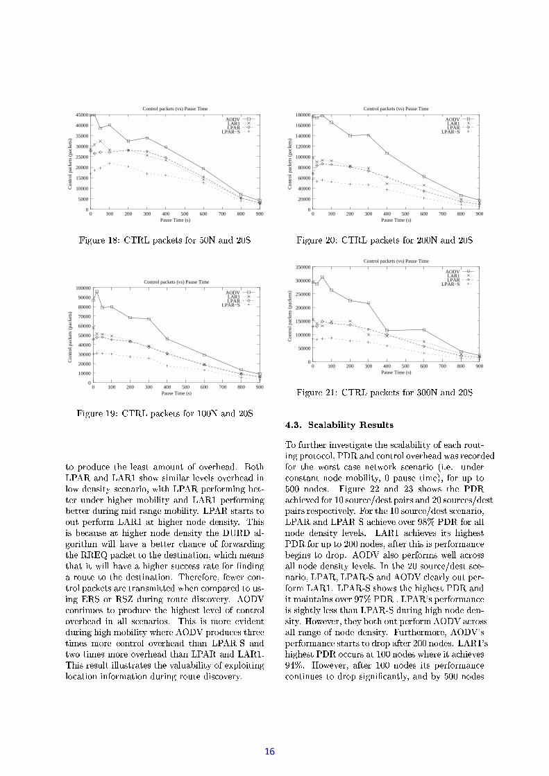
ÁfÆ!º½fÆZÑZÒKÓ¡¼ªÁf¶¼Å¼»I¸¿Á»#ÍÆIÒÀÁÆ Û Æ>ÙI¼¡½f¶¼»IÑTß ãÆIÁ¾¶ÖdÈT×lÚ*»IÀKÑÖ@×ØÚ a¸¾¶Æ>Ã9¸¾·Í·LÅL»I½ØÅL¼¡Ù(¼¡Å¹¸ÝÆ>ÙI¼B½¾¶K¼B»IÑ·LÀÅLÆ>ÃÑZ¼BÀK¸¾·Á˸¾Ó¡¼¡ÀK»I½¾·LÆKÕZè·Á¾¶ÖdÈT×lÚXºD¼¡½ Û ÆI½fÍ¥·LÀÉ-ÇD¼ÔÁ¾ÌÁf¼¡½¥ÒÀKÑZ¼B½a¶·LÉI¶K¼¡½1ÍÆ(Ç·ÅL·ÁË»IÀKÑ'Öd×lÚ ªºz¼B½ Û Æ(½¾Í·LÀÉÇD¼ÔÁ¾Á¾¼¡½ÑZÒ½f·LÀɳͷLѽf»IÀÉI¼ÝÍÆ(Ç·ÅL·ÁËIßvÖ@ÈT×lÚF¸Á»#½¾Áf¸ÁfÆÆ(ÒZÁ1ºD¼¡½ Û ÆI½fÍüÖ@×ØÚ ª»#Á1¶·LÉI¶¼B½³ÀÆZÑZ¼¯Ñ¼¡ÀK¸¾·ÁË(ßµ¶·¹¸·¹¸hÇD¼BÓ¡»IÒK¸¾¼»>Á1¶·LÉI¶K¼¡½³ÀÆZÑZ¼ªÑZ¼¡ÀK¸¾·ÁËÁ¾¶K¼ªýõlÚÝý »#ÅÌÉ(ÆI½f·Áf¶Í è·ÅLŨ¶K»Ù(¼ª»Çz¼¡Á¿Áf¼¡½Ó¶K»IÀKÓÔ¼Æ ÛØÛ ÆI½fÃã»I½fÑZ·LÀÉÁf¶¼¨ÚÝÚÝô ú ºK»IÓÂÞ(¼ÔÁ@ÁfÆÁ¾¶¼¨ÑZ¼¸Áf·ÀK»#Á¾·LÆIÀÕI趷LÓ¶aͼB»#Àz¸Áf¶K»>Á`·Á`è·LÅŶK»Ù(¼a»¯¶·É(¶¼¡½h¸¾ÒKÓ¡Ó¡¼B¸f¸l½Â»>Áf¼ Û Æ(½Ø÷zÀKÑZ·LÀÉ»¯½¾Æ(ÒZÁ¾¼aÁ¾ÆªÁ¾¶¼-ÑZ¼¸Áf·Àz»>Á¾·LÆIÀ@ß1µ¶¼¡½f¼ Û Æ(½¾¼(Õ Û ¼¡Ã㼡½hÓÔÆ(ÀZÌÁf½¾Æ(Å(ºK»(ÓÂÞI¼¡Áf¸@»I½¾¼RÁ¾½Â»#ÀK¸¾Í·Á¾Á¾¼BÑ1趼¡À¥ÓÔÆ(Í¥ºz»#½f¼BÑÁ¾ÆØÒK¸¿Ì·LÀÉôÏÚlÊÆI½aÚlÊÑZÒK½¾·LÀɽfÆIÒÁ¾¼¯ÑZ·¹¸fÓÔÆ>ÙI¼B½¾Ë(ß×læý¨þÓ¡ÆIÀÁ¾·LÀ£Ò¼B¸`Áfƺ½fÆZÑZÒKÓ¡¼-Á¾¶¼ª¶·LÉI¶¼¸Á1ÅL¼¡Ù(¼¡ÅÏÆ Û ÓÔÆ(À(Áf½¾Æ(ÅÆ>Ù(¼¡½f¶¼B»(Ñ'·LÀF»#ÅLÅظfÓÔ¼BÀK»#½f·LÆ(¸BßXµ¶·¹¸ª·L¸¯Í¥Æ(½¾¼¼¡Ù£·LѼ¡ÀÁÑZÒK½¾·LÀÉ`¶·LÉI¶¥Í¥Æ(Ç·LÅ·ÁË1趼B½¾¼¨×læý¨þºK½¾ÆZÑZÒKÓ¡¼B¸MÁf¶½¾¼B¼Áf·Í¼B¸ÍÆI½f¼ÓÔÆIÀÁf½¾Æ(ÅÆ>Ù(¼¡½f¶¼B»(Ñ Á¾¶K»IÀXÖdÈT×lÚÌÊ»IÀKÑÁÃãÆÁ¾·LͼB¸ØÍ¥Æ(½¾¼1Æ>ÙI¼¡½f¶¼»IѯÁ¾¶K»IÀÖ@ÈT×lÚ »#ÀKÑÖd×lÚ (ßµ¶·¹¸Ï½¾¼¸¿ÒÅÁÏ·LÅLÅÒK¸¿Á¾½Â»>Áf¼B¸ÜÁ¾¶¼Ù>»#ÅLÒK»#ÇK·ÅL·ÁËÆ Û ¼ÔáZºÅLÆI·Á¾·LÀÉÅLÆZÓ¡»>Áf·Æ(À¯·LÀ Û ÆI½fÍ-»>Áf·Æ(ÀÑZÒK½¾·LÀÉ-½fÆIÒZÁf¼`Ñ·L¸fÓÔÆ>Ù(¼¡½fËIß

0

20000

40000

60000

80000

100000

120000

140000

160000

180000

0 100 200 300 400 500 600 700 800 900

Con

trol

pac

kets

(pa

cket

s)

Pause Time (s)

Control packets (vs) Pause Time

AODVLAR1LPAR

LPAR−S

çM·LÉIÒ½f¼ *# 㵨ÚlÖ!ºz»IÓÂÞI¼¡Áf¸ Û Æ(½ *#4#(ó»IÀKÑ *#Ê

0

50000

100000

150000

200000

250000

300000

350000

0 100 200 300 400 500 600 700 800 900

Con

trol

pac

kets

(pa

cket

s)

Pause Time (s)

Control packets (vs) Pause Time

AODVLAR1LPAR

LPAR−S

çM·LÉIÒ½f¼ 㵨ÚlÖ!ºz»IÓÂÞI¼¡Áf¸ Û Æ(½Ýà4#4#(ó»IÀKÑ *#Ê

/dë @ë °(4& 39&21 + 3-+-) s² $52303-)2µdÆ Û Ò½¾Á¾¶¼B½Ï·LÀ£ÙI¼¸Áf·É»>Á¾¼ÝÁ¾¶¼¸¾ÓB»#Ź»#Ç·LÅ·ÁË¥Æ Û ¼»IÓ¶-½fÆIÒZÁ¾Ì·LÀɨº½fÆ#Á¾ÆZÓ¡ÆIÅ^ÕBÈÜýÚ»#ÀzÑÓ¡ÆIÀÁ¾½fÆIÅ>Æ>Ù(¼¡½f¶¼B»(ÑÝûI¸r½f¼BÓ¡ÆI½ÂÑZ¼BÑÛ ÆI½¯Á¾¶¼!ÃÏÆ(½f¸¿Á¯Ó¡»(¸¿¼ÀK¼ÔÁÃãÆI½fÞ ¸fÓÔ¼BÀK»#½f·Æηnß ¼Iß*ÒKÀKÑZ¼¡½ÓÔÆ(ÀK¸¿Áf»#ÀÁ³ÀÆZÑZ¼-ÍÆ(Ç·ÅL·ÁËIÕ #ºK»#ÒK¸¾¼Á¾·LͼÐÔÕ Û Æ(½³ÒºÁfÆ*# #ÀÆZÑZ¼B¸BßâçM·LÉIÒ½f¼ »IÀKÑ I฿¶KÆ>ÃݸÁ¾¶¼ ÈÜýÚ»IÓ¶K·¼BÙI¼BÑ Û ÆI½ #¸¿Æ(Ò½ÂÓÔ¼#ÑZ¼B¸¿ÁTºK»#·L½Â¸T»#ÀKÑ 4#㸾ÆIÒK½fÓ¡¼B¸>ÑZ¼¸ÁºK»I·½Â¸T½f¼B¸¾ºz¼ÓÁ¾·LÙI¼BÅË(ß@çÆ(½TÁ¾¶K¼ #¨¸¾ÆIÒ½ÂÓÔ¼b>ÑZ¼¸Á¸fÓÔ¼BÀK»#½f·ÆzÕÖ@ÈT×ØÚF»IÀKÑÖ@ÈT×ØÚÌÊ»IÓ¶K·¼BÙI¼ÝÆ>Ù(¼¡½ <ÈÜýÚ Û Æ(½ã»IÅÅÀÆZÑZ¼ÑZ¼BÀK¸¿·ÁËÅL¼¡ÙI¼BÅL¸Bß Öd×lÚ »(Ó¶·¼BÙI¼¸¯·Áf¸¶·LÉI¶K¼B¸¿ÁÈÜýÚ Û Æ(½dÒKº³Á¾Æ *# #¨ÀÆZÑZ¼¸¡Õ#» Û Á¾¼¡½dÁ¾¶K·L¸v·¹¸@ºD¼¡½ Û ÆI½fÍ-»#ÀKÓ¡¼ÇD¼¡ÉI·LÀK¸ØÁ¾ÆÑZ½fÆIº@ß1×læý¨þå»#Ź¸¿Æºz¼B½ Û Æ(½¾Í-¸Ã㼡ÅLÅv»(ÓÔ½fÆ(¸f¸»#ÅLÅTÀÆZÑZ¼³ÑZ¼BÀK¸¾·Á˪żBÙI¼¡Å¹¸BßäeÀªÁf¶¼ 4#¥¸¾ÆIÒK½fÓ¡¼>ѼB¸¿Á¸fÓÔ¼¡ÌÀK»I½¾·LÆKÕ#ÖdÈT×lÚhÕ#ÖdÈT×lÚÌÊ1»IÀKÑ¥×læý¨þÓÔÅL¼B»#½fÅLËhÆIÒZÁºD¼¡½¾ÌÛ ÆI½fÍ Ö@×ØÚ IßÖ@ÈT×ØÚÌÊ-¸¿¶KÆ>ÃݸÁ¾¶K¼Ø¶·LÉI¶K¼B¸¿ÁãÈÜýÚ»IÀKÑ·ÁvÍ-»I·ÀÁf»I·Àz¸dÆ>Ù(¼¡½ 'FÈÏýØÚß#Ö@ÈT×ØÚhé ¸dºD¼¡½ Û ÆI½fÍ-»#ÀKÓ¡¼·¹¸R¸¿·LÉI¶ÁfÅËaż¸¾¸MÁf¶K»#ÀÖdÈT×lÚÌÊ¥ÑZÒ½f·ÀÉh¶K·É(¶¥ÀKƣѼÝÑZ¼¡ÀZ̸¾·ÁË(ß@ùÝÆ>Ã㼡Ù(¼¡½ÕÔÁ¾¶K¼¡ËlÇDÆ#Áf¶hÆIÒZÁºD¼¡½ Û ÆI½fÍ×læýÝþ'»IÓ¡½¾Æ¸¾¸»#ÅLŽ»#ÀÉ(¼aÆ Û ÀÆZÑZ¼-ÑZ¼BÀK¸¿·ÁËIß-çKÒ½¿Áf¶¼¡½fÍÆI½f¼IÕ×læý¨þaé ¸ºD¼¡½ Û ÆI½fÍ»IÀKÓÔ¼¸¿Áf»I½¿Á¸rÁ¾ÆÝÑZ½fÆIºh» Û Á¾¼¡½ *#4#ãÀÆZÑZ¼¸¡ßdÖ@×lÚ Ié ¸¶·LÉI¶¼¸ÁvÈÜýÚÆZÓ¡Ó¡Ò½f¸d»>Á #4#ÝÀÆZÑZ¼B¸d趼¡½f¼R·Áv»(Ó¶·L¼¡ÙI¼¸ ¯ß ùlÆ>ÃϼBÙI¼¡½ÕÜ» Û Á¾¼¡½ 3#4#!ÀÆZÑZ¼B¸·Áf¸ºD¼¡½ Û ÆI½fÍ-»#ÀKÓ¡¼ÓÔÆ(ÀÁ¾·LÀÒK¼B¸lÁ¾ÆªÑ½¾Æ(º¸¿·LÉIÀK·÷zÓB»#ÀÁ¾ÅLËIÕT»IÀKÑÇ£Ë*# #-ÀÆZÑZ¼B¸

80

85

90

95

100

50 100 150 200 250 300 350 400 450 500

Pack

et D

eliv

ery

Rat

io (

%)

Number of Nodes

Packet Delivery Ratio (vs) Number of Nodes

LPARLPAR−S

LAR1AODV

çM·LÉIÒ½f¼ vÈÏýØÚ Û ÆI½¨ºz»#ÒK¸¾¼`Á¾·Lͼ% #»#ÀKÑ 3#(Ê

80

85

90

95

100

50 100 150 200 250 300 350 400 450 500

Pack

et D

eliv

ery

Rat

io (

%)

Number of Nodes

Packet Delivery Ratio (vs) Number of Nodes

LPARLPAR−S

LAR1AODV

çM·LÉIÒ½f¼ #àÈÏýØÚ Û ÆI½¨ºK»IÒK¸¾¼ØÁf·Í¼%J#»#ÀzÑ 4#(Ê

·Áݺz¼B½ Û Æ(½¾Í-»IÀKÓÔ¼¶K»I¸¨Ñ½¾Æ(ººz¼ÑªÁ¾Æ IàßçM·LÉIÒ½f¼ »#ÀKÑ 4 ¸¾¶Æ>ÃݸªÁ¾¶¼À£ÒÍaÇz¼B½Æ Û ÓÔÆ(À(Áf½¾Æ(źK»(ÓÂÞI¼¡Áf¸r·LÀ(Áf½¾ÆZÑZÒzÓÔ¼BÑ·LÀÁ¾ÆÁ¾¶K¼RÀ¼ÔÁÃãÆI½fÞ Û Æ(½ #¨¸¾½fÓ>ÑZ¼¸ÁºK»I·½Â¸v»#ÀKÑ *#¸¾ÆIÒ½ÂÓÔ¼¸L#ÑZ¼B¸¿ÁdºK»I·½Â¸M½¾¼¸¿ºD¼BÓÔÁ¾·LÙI¼BÅË(ßdç½fÆIÍÁf¶¼B¸¾¼`÷KÉIÒK½¾¼¸·ÁØÓB»#ÀÇD¼1¸¿¼B¼¡ÀÁ¾¶z»>ÁØ»(¸Á¾¶¼1ÀÆZÑZ¼³ÑZ¼¡À̸¾·ÁËF·L¸·LÀKÓ¡½¾¼»I¸¾¼BÑÁf¶¼ºD¼¡½ Û ÆI½fÍ»IÀKÓÔ¼ÑZ·ör¼¡½f¼¡ÀKÓ¡¼Çz¼¡ÌÁÃ㼡¼BÀª¼»IÓ¶½¾Æ(ÒZÁ¾·LÀÉ-¸¿Á¾½Â»>Á¾¼BÉIËÇD¼BÓ¡ÆIͼB¸ÝÍ¥Æ(½¾¼h¸¾·É(À· Û Ì·¹Ó¡»IÀ(ÁßF×læý¨þ ¶z»I¸-¶·LÉI¶K¼¡½ÓÔÆ(ÀÁ¾½fÆIÅÝÆ>Ù(¼¡½f¶¼B»(ÑÁ¾¶z»#ÀÖd×lÚ (ÕÖdÈT×lÚ»#ÀKÑ`ÖdÈT×lÚÌÊ Û ÆI½ÇDÆ#Áf¶`Á¾¶¼ 3#¸¿½ÂÓ3#ÑZ¼B¸¿Á¸fÓÔ¼BÀK»#½f·ÆØ»#ÀKÑ1Á¾¶¼ 4#ظ¾½fÓ>ÑZ¼¸Áv¸¾Ó¡¼¡ÀK»I½¾·LÆlè¶K¼¡½f¼Ï·Áº½¾ÆIÌÑZÒzÓÔ¼B¸ªÁf¶½¾¼B¼Á¾·LÍ¥¼¸ÍÆI½f¼!Æ>Ù(¼¡½f¶¼B»(ÑÁ¾¶K»IÀXÖdÈT×lÚÌÊ»IÀKÑhÆ>ÙI¼B½TÁÃãÆÝÁ¾·LͼB¸dÍÆI½f¼RÆ>ÙI¼B½¾¶¼»IÑÁf¶K»#À1ÖdÈT×lÚ»IÀKÑÖd×lÚ (ß<Ö@ÈT×ØÚÌÊÓÔÆ(À(Áf·À£Ò¼¸-ÁfÆ'º½fÆZÑZÒKÓÔ¼Á¾¶¼!ż»I¸¿Á»IÍ¥Æ(ÒÀÁÝÆ Û Æ>ÙI¼B½¾¶¼»IÑ Û ÆI½l»IÅÅdÀÆZÑZ¼³ÑZ¼¡Àz¸¿·Á˪¸fÓÔ¼BÀK»#½f·ÆzßÖdÈT×lÚ »#Ź¸¿Æh¸¾¶Æ>Ãݸ Û ¼¡Ã㼡½RÆ>Ù(¼¡½f¶¼B»(Ѹ@Á¾¶K»IÀÖd×lÚ Ý»IÀKÑ×læý¨þaßݵ¶¼¡½f¼ Û Æ(½¾¼(Õ Û ½fÆIÍ%Áf¶¼B¸¾¼½¾¼¸¿ÒÅÁf¸·ÁÓ¡»IÀFÇD¼¸¾¼¡¼BÀÁ¾¶z»>ÁÇzÆIÁ¾¶Ö@ÈT×lÚX»#ÀzѯÖ@ÈT×ØÚÌÊ»#½f¼lÍÆ(½¾¼`¸¾ÓB»#ÅÌ»IÇżÁf¶K»#À×læý¨þ*»IÀKÑÖ@×lÚ ³»I¸Áf¶¼hżBÙI¼BÅTÆ Û Á¾½Â»>ûÓ»IÀKѯÀKƣѼ³ÑZ¼¡ÀK¸¾·ÁË·ÀzÓÔ½f¼B»I¸¾¼B¸ã·LÀÁ¾¶¼hÀ¼¡ÁÃÏÆ(½¾Þrß

/dë0/dë ï$3-& ²%$'230 3 )2çM·LÉIÒ½f¼ 4 l»#ÀzÑ Ý¸¿¶Æ>Ãݸ@Á¾¶K¼ã»Ù(¼¡½Â»#ÉI¼¼BÀKÑ£Ì^Á¾ÆIÌ^¼BÀKѳÑZ¼¡ÌŹ»ËݼÔáZºD¼¡½f·¼BÀKÓÔ¼Ñ`Ç£Ël¼B»(Ó¶hÑ»>Á»ºK»IÓÂÞ(¼ÔÁ Û ÆI½ 3#¨¸¿½ÂÓ3#ÑZ¼B¸¿Á

0

20000

40000

60000

80000

100000

120000

140000

50 100 150 200 250 300 350 400 450 500

Num

ber

of C

ontr

ol p

acke

ts

Number of Nodes

CTRL packets (vs) Number of Nodes

LPARLPAR−S

LAR1AODV

çM·É(Ò½¾¼ 㵨ÚÝÖ Û ÆI½¨ºK»IÒK¸¾¼`Á¾·LÍ¥¼%J#¥»#ÀzÑ 3#(Ê

0

100000

200000

300000

400000

500000

600000

700000

50 100 150 200 250 300 350 400 450 500

Num

ber

of C

ontr

ol p

acke

ts

Number of Nodes

CTRL packets (vs) Number of Nodes

LPARLPAR−S

LAR1AODV

çM·É(Ò½¾¼ 㵨ÚÝÖ Û ÆI½¨ºK»IÒK¸¾¼`Á¾·LÍ¥¼%J#¥»#ÀzÑ 4#(Ê

ºK»I·½Â¸»#ÀKÑ *# ¸¾½fÓ>ÑZ¼¸ÁºK»I·½Â¸·À9» # #sÀKƣѼÀK¼ÔÁ¿ÌÃãÆI½fÞ½¾¼¸¿ºD¼BÓÔÁ¾·LÙI¼¡ÅLËIß-×ظ`¼ÔáZºz¼ÓÁf¼BÑTÕM»#ÅLÅRº½fÆ#Á¾ÆZÓ¡ÆIŹ¸Ø¼¡á£ÌºD¼¡½f·¼BÀKÓÔ¼Ñ1Ź»#½fÉI¼B½vѼ¡Å¹»Ë£¸ÑÒ½¾·LÀÉ`¶·LÉI¶ÍÆIÇ·LÅL·ÁË(ÕI¸¿·LÀKÓ¡¼ÍÆI½f¼ Û ½f¼Ò¼BÀ(Á`ÅL·ÀÞ Û »I·ÅLÒ½f¼aÍ-»ËÓB»#ÒK¸¾¼1½fÆIÒZÁf¼a½f¼BÓB»#ÅÌÓÔÒKÅL»#Á¾·LÆIÀßµ¶·¹¸Üͼ»#ÀK¸ÜÁ¾¶K»IÀ¯¼»IÓ¶-ºK»(ÓÂÞI¼ÔÁãÍ-»Ëa¼¡á£ºD¼Ô̽f·¼BÀKÓÔ¼`ÅLÆIÀÉ(¼¡½ÝÑZ¼BÅL»ËZ¸ÇD¼ Û ÆI½f¼`Á¾¶K¼¡Ë¯½f¼B»(Ó¶¯Áf¶¼¡·L½lÑZ¼¸Áf·ÌÀK»#Á¾·LÆIÀßh×læý¨þ<¶K»I¸ØÅÆ>Ãã¼B¸¿ÁؼBÀKÑ£Ì^Á¾ÆIÌ^¼BÀKÑÑZ¼BÅL»ËÓÔÆ(̺ͥK»I½¾¼ÑÁfÆÁ¾¶¼ÆIÁ¾¶¼B½º½¾ÆIÁ¾ÆZÓÔÆ(ÅL¸Bß µ¶·¹¸·L¸Çz¼Ó¡»#Òz¸¿¼(Õ×læý¨þ»#ÅLûˣ¸MÒK¸¾¼B¸MÁf¶¼Ý¸¾¶ÆI½¾Á¾¼¸Á½fÆIÒZÁf¼ÏÁfÆÁ¾¶¼ÝÑZ¼¸Áf·ÌÀK»#Á¾·LÆIÀh»#ÀKÑ·Á@ÆIÀKÅËØÍ»I·ÀÁ»#·LÀK¸»¨¸¾·ÀÉ(żv½fÆIÒZÁf¼IÕ趼¡½f¼B»(¸Ö@×ØÚ aÓB»#À¸¿Á¾Æ(½¾¼1Í1ÒÅÁ¾·LºÅL¼a½fÆIÒZÁf¼Iß`µ¶·¹¸lͼB»IÀK¸lÁ¾¶K»#Á· Û Æ(ºZÁ¾·LÍ-»#Ũ½fÆIÒZÁf¼ Û »I·Å¹¸Î Áf¶¼ÆIÀK¼ªÃ¨·Á¾¶ Á¾¶K¼¸¿¶Æ(½¿Áf¼B¸¿Á¸¾½fÓ>ÑZ¼¸ÁݺK»#Á¾¶zÐÔÕT»#À»#ÅÁ¾¼B½¾Àz»>Á¾¼1½¾Æ(ÒZÁ¾¼ Û ½fÆIÍ Áf¶¼1½fÆIÒZÁf¼Ó¡»(Ó¶¼1Í-»ËÇD¼ÒK¸¿¼(ß1µ¶·¹¸`ͼB»#Àz¸lÁf¶K»>Áh¸¾ÆIͼaºz»IÓÂÞI¼¡ÁÍ-»ËÁ¾½Â»ÙI¼BÅÆ>ÙI¼B½ÅLÆIÀKÉI¼¡½`½fÆIÒZÁf¼B¸Áfƽ¾¼»IÓ¶!Á¾¶¼ÑZ¼¸Áf·ÌÀK»#Á¾·LÆIÀßÊ£·LÍ¥·LŹ»#½fÅ˳·LÀÖ@ÈT×ØÚs»IÀKÑÖ@ÈT×ØÚÌeÊa· Û Áf¶¼Ýº½f·ÌÍ-»#½fË-½¾Æ(ÒZÁ¾¼ Û »#·LŹ¸¡ÕZ¸¾ÆIͼغz»IÓÂÞI¼¡ÁãÍ-»ËÁf½f»Ù(¼¡ÅDÆ>ÙI¼¡½ÏÁ¾¶K¼¸¾¼BÓÔÆ(ÀKÑ»I½¾Ë½fÆIÒÁ¾¼IÕd趷¹Ó¶ͻË!Çz¼¯ÅÆ(ÀÉI¼B½h·ÀÅL¼¡ÀÉIÁ¾¶ßµ¶¼B½¾¼ Û ÆI½f¼IÕÁ¾¶K¼¡Ë1Í-»Ë³¼¡áZºz¼B½¾·L¼¡ÀKÓ¡¼Ý¸¿ÅL·LÉI¶Á¾ÅL˳ÅLÆIÀÉ(¼¡½ÑZ¼ÔÌŹ»ËIßhç½fÆIÍ Á¾¶K¼a÷zÉIÒ½f¼B¸ØÃϼ¥Ó¡»IÀ!¸¾¼¡¼³Áf¶K»>ÁhÖ@ÈT×ØÚ »IÀKÑÖ@ÈT×ØÚÌʶK»Ù(¼ÆIÀ »ÙI¼¡½Â»#É(¼»#ÇDÆIÒZÁ">Í-¸¥ÍÆI½f¼ªÑZ¼BÅL»Ë»IÓ¡½¾Æ¸¾¸»IÅÅݽ»#ÀKÉI¼Æ Û ÍÆIÇ·LÅ·ÁËIßXùÝÆ>Ã㼡Ù(¼¡½ÕÜÇ£Ë'ÒK¸¾·LÀÉ»¸¿¼ÓÔÆ(ÀKÑ»#½f˽fÆIÒZÁf¼IÕÖ@ÈT×lÚ »IÀKÑsÖdÈT×lÚÌÊ »#½f¼»IÇÅL¼Á¾Æ¸¾ÒKÓBÓÔ¼B¸f¸ Û ÒÅÅLËÁf½f»IÀK¸¿Í·ÁÍÆI½f¼ÑK»>Áf»ºz»IÓÂÞI¼¡Áf¸BÕÏ»IÀKÑ

0.04

0.045

0.05

0.055

0.06

0.065

0 100 200 300 400 500 600 700 800 900

End

−to

−E

nd D

elay

(s)

Pause Time (s)

End−to−End Delay (vs) Pause Time

AODVLAR1LPAR

LPAR−S

çM·LÉIÒ½f¼ * ×lÙI¼¡½Â»#É(¼ôÜÀKÑ£Ì^Á¾ÆIÌ^¼BÀKѪѼ¡Å¹»Ë Û ÆI½ 3#(Ê

0.04

0.05

0.06

0.07

0.08

0.09

0.1

0.11

0.12

0 100 200 300 400 500 600 700 800 900

End

−to

−E

nd D

elay

(s)

Pause Time (s)

End−to−End Delay (vs) Pause Time

AODVLAR1LPAR

LPAR−S

çM·LÉIÒ½f¼ ×lÙI¼¡½Â»#É(¼ôÜÀKÑ£Ì^Á¾ÆIÌ^¼BÀKѪѼ¡Å¹»Ë Û ÆI½ 4#(Ê

½f¼BÑZÒzÓÔ¼³Áf¶¼¥ÀÒKÍ1ÇD¼¡½`Æ Û ½fÆIÒÁ¾¼1½f¼BÓB»#ŹÓÔÒŹ»>Áf·Æ(ÀK¸BÕz趷¹Ó¶ͼB»IÀK¸ Û ¼¡Ã㼡½ÝÓ¡ÆIÀÁ¾½fÆIÅrºK»(ÓÂÞI¼¡Áf¸Bß

Të î ± ì*ì °@­`± ì î í °­ í ïì ²î í ±a°

äeÀÁf¶·¹¸ªºz»#ºD¼¡½ÕÝÃϼ!¶K»ÙI¼!·ÀÁf½¾ÆZÑZÒKÓ¡¼BÑ»'À£ÒÍ1ÇD¼¡½Æ ÛÑZ·ör¼¡½f¼¡ÀÁv¸¿Á¾½Â»>Áf¼¡É(·¼¸TÁ¾Æ½f¼BÑZÒKÓ¡¼Ü½fÆIÒZÁf·ÀKÉlÆ>ÙI¼B½¾¶K¼B»IÑh»IÀKѺDÆ>ÃϼB½@ÒK¸¾¼BÑ¥ÑZÒ½f·LÀÉl½fÆIÒZÁf¼ãÑ·L¸fÓÔÆ>Ù(¼¡½fËIßTäeÀaÁ¾¶·¹¸v¸¿¼ÓÁ¾·LÆIÀ@ÕÃã¼ÜÑZ¼¸¾Ó¡½¾·LÇz¼Ï»¨À£ÒÍ1ÇD¼¡½MÆ Û ÑZ·öD¼B½¾¼BÀÁdÆIºÁ¾·LÍ¥·¹¸f»>Á¾·LÆIÀ³»IÀKÑ×lÅÁf¼¡½fÀK»>Áf·Ù(¼³¸Áf½f»#Á¾¼¡É(·¼¸¡ÕK趷LÓ¶ÓB»#À Û Ò½¾Á¾¶K¼¡½l·Lͺ½fÆ>ÙI¼Áf¶¼hºz¼B½ Û Æ(½¾Í-»IÀKÓÔ¼Æ Û Ö@ÈT×ØÚhß

ëêDë Ð1/7PÑ & 7£ÍB+ 1 + 39+ ) s­ 3-:6/7b+ ) /.7¯ï𪲪ïäeÀÁ¾¶K¼ÜýØõØÚÝý »#ÅLÉIÆI½f·Á¾¶Í În¸¿¼ÓÁf·Æ(À ß (ÐÕÚÝÚÝô ú ºK»(ÓÂÞ(̼¡Áf¸»I½¾¼ Û Æ(½¾Ã»#½ÂÑZ¼BÑ'Á¾Æ>û#½ÂѸ¥Áf¶¼!ÑZ¼¸Áf·Àz»>Á¾·LÆIÀÒK¸¾·LÀÉÁf¶¼¨·ÀÁf¼¡½fÍ¥¼ÑZ·¹»>Á¾¼¨ÀKƣѼB¸Ã¨¶·¹Ó¶-¶K»Ù(¼»`Í·LÀ·LÍ1Òͽ¾¼¡ÌÒ·L½¾¼Ñ!Ѽ¡ÉI½f¼¡¼Î ·^ß ¼IßÀÆZÑZ¼ÑZ¼BÀK¸¿·ÁËIÕ@ÃϼÒK¸¾¼ Ê ·LÀÁ¾¶·¹¸ÜÓB»I¸¾¼Ð»IÀKÑ¥Á¾¶K¼Ý·ÀÁf¼¡½fÍ¥¼ÑZ·¹»>Á¾¼ØÑZ·L¸¿Áf»IÀKÓÔ¼¨·¹¸RÅL¼B¸f¸Áf¶K»#ÀTßaµ@Æ Û Ò½¿Áf¶¼¡½`·LÀKÓÔ½f¼B»(¸¿¼³Á¾¶¼¥ºzƸ¾¸¾·LÇ·ÅL·ÁËÆ Û Áf¶¼ OA GETM9A>;9UVADFG Z MA F3Gc9MZLE_DA Gc;M9OA FGc-MaZLE_DA W*ASMY\;ADAE M9OA

K I;-\ Z7;F3GEH EI FA ZLEF>MO3A E3A<I M1EIF3A \1O3G_aOJGc _aOIc9ADE[ZLcM9OAEAIM K I;9\ Z7;9FGEH EIF3A

A(x,y)

(x,y+r)

(x−r,y) (x+r,y)

r

(x,y−r)

θ

B

N

S

EW

çM·É(Ò½f¼ * ãýطͼBÀK¸¿·LÆIÀz¸lÒK¸¾¼BÑÁ¾Æ ã»IÅLÓ¡ÒŹ»>Á¾¼³Á¾¶¼ Û ÆI½¾Ìû#½ÂÑ»#Ç·LÅL·ÁË Û »(ÓÁ¾Æ(½

ÚÝÚÝô ú ºK»(ÓÂÞI¼ÔÁ¸¯½f¼B»(Ó¶·LÀÉÁf¶¼ÑZ¼B¸¿Á¾·LÀK»>Áf·Æ(ÀηÀÁ¾¶K¼ýõlÚÝý »IÅÉ(ÆI½f·Áf¶ÍÐÕDÃϼa·ÀÁ¾½fÆZÑZÒKÓ¡¼a» Û Æ(½¾Ã»#½ÂÑ»IÇ·ÅL·ÁË»#ÅLÉIÆ(½¾·Á¾¶KÍÕDÁfÆ»IÅÅLÆ>Ã9Á¾¶K¼ Û Æ(½¾Ã»#½ÂÑZ·LÀÉÀÆZÑZ¼¥ÁfƪÍ-»#Þ(¼Û Ò½¾Á¾¶¼B½ÏÑZ¼ÓÔ·¹¸¿·LÆIÀz¸R»#ÇDÆIÒZÁÏ趼ÔÁf¶¼¡½ÜÁ¾¶¼ÝÀK¼Ôá£Á Û ÆI½fû#½Âѣ̷LÀÉ-ÀÆZÑZ¼1Ó¶Ƹ¿¼BÀ·L¸Ý»IÇÅL¼hÁ¾Æ Û Æ(½¾Ã»#½ÂÑÁf¶¼aÚlÚÝô ú Á¾ÆIÌû#½ÂѸãÁ¾¶¼¥ÑZ¼B¸¿Á¾·LÀK»#Á¾·LÆIÀßµ@ƪÑZÆÁ¾¶·¹¸BÕz¼»IÓ¶ÀÆZÑZ¼1ÓB»#ÅÌÓÔÒKÅL»#Á¾¼B¸1» Û Æ(½¾Ã»#½ÂÑZ·LÇ·LÅ·ÁË Û »IÓÔÁ¾Æ(½Î ·LÀK¸Áf¼B»(Ñ!Æ Û »ÀKƣѼÑZ¼BÉI½f¼¡¼Ð`»IÀKѼÔáÓ¶K»IÀÉI¼¸Á¾¶·¹¸a·À Û Æ(½¾Í-»#Á¾·LÆIÀè·Áf¶Á¾¶K¼À¼B·É(¶ÇDÆIÒK½¾·LÀÉÝÀÆZÑZ¼¸IßMµdÆØѼB¸fÓÔ½f·ÇD¼RÁf¶¼ Û Æ(½¾Ã»#½ÂÑ»#ÇK·ÅÌ·ÁËs»#ÅLÉIÆ(½¾·Á¾¶KÍÕÃã¼½¾¼ Û ¼¡½-ÁfÆ'çM·É(Ò½f¼ *ßñµdÆÓ¡»#ŹÓÔÒÌŹ»>Á¾¼ÝÁ¾¶¼ Û ÆI½fÃã»I½fÑZ·LÇ·LÅ·ÁËIÕI¼B»IÓ¶-ÀKƣѼlÑZ¼Ô÷zÀ¼B¸ã¸Á»#½¾Áf¸Ç£ËÑZ¼¡÷KÀ·LÀÉ Û ÆIÒK½lºDÆI·LÀ(Á`»>ÁØ»ªÑZ·¹¸Á»#ÀKÓ¡¼1Ú9»Ãã»Ë Û ½¾Æ(Í ·Áf¸ÓÔÒK½¾½f¼¡ÀÁÝÅLÆ£ÓB»>Áf·Æ(Àß㵶K¼B¸¾¼³ºzÆ(·ÀÁ¸l»#½f¼³»>ÁØÀÆI½¾Á¾¶Õz¼B»(¸ÁÕ¸¾ÆIÒZÁf¶a»#ÀzѳÃã¼B¸¿Áv»(¸d¸¾¶Æ>èÀ³·LÀ¥çM·LÉIÒ½f¼ 4ßMõl¸¾·ÀÉØÁ¾¶K¼B¸¾¼ºDÆI·LÀ(Á¸`Á¾¶K¼-ÀÆZÑZ¼B¸`è·LÅÅÏÑZ¼ÔÁf¼¡½fÍ¥·LÀ¼-· Û Áf¶¼¡Ë!¶K»ÙI¼-»IÀËÀ¼B·É(¶ÇDÆIÒK½-趷LÓ¶ÅL¼B»(ÑsÁ¾ÆÎ Æ(½¯»#ºKº½¾ÆáZ·LÍ-»>Á¾¼BÅËÅL¼B»(ÑÁ¾Æ£ÐØÁ¾¶Æ¸¿¼Ñ·½f¼BÓÔÁ¾·LÆIÀK¸BÕ@ÒK¸¾·LÀÉÁ¾¶¼B·½aÀ¼¡·LÉI¶£ÇDÆIÒ½`Á»#ÇÅL¼Ißµ¶·¹¸M·L¸ÑZÆ(À¼ãÇË1Í»Iºº·LÀɼB»IÓ¶aÀ¼¡·LÉI¶£ÇDÆIÒ½v·LÀ1Áf¶¼¨ÓÔÆIÌÆI½ÂÑZ·LÀK»>Áf¼ÜºÅ¹»#ÀK¼IÕI»IÀKÑ1ÑZ¼¡Á¾¼B½¾Í·LÀ·ÀKÉØ趷¹Ó¶1ÀK¼¡·LÉI¶£ÇzÆ(ҽ¸»#½f¼ÓÔÅLÆ(¸¾¼B¸¿ÁØÁfÆè¶K·LÓ¶!ÆIÀ¼Æ Û Á¾¶¼ Û Æ(Ò½`ºzÆ(·ÀÁf¸Bßµ¶·L¸Ó¡»IÀ¯ÇD¼³ÑZÆIÀK¼¼B·Áf¶¼¡½¨Ç£ËÓ¡ÆIͺK»#½f·LÀÉ1Áf¶¼hÑZ·¹¸Á»#ÀKÓ¡¼ÇD¼ÔÌÁÃ㼡¼¡À-¼»IÓ¶-À¼B·É(¶£ÇzÆ(Ò½Üè·Á¾¶¼»IÓ¶-Æ Û Á¾¶¼ Û ÆIҽϺzÆ(·ÀÁf¸ÆI½`Ó¡»IÅLÓ¡ÒŹ»>Á¾·LÀÉ-Áf¶¼»#ÀÉ(ż ¯ÇD¼ÔÁÃ㼡¼¡ÀÁ¾¶¼¥À¼B·É(¶ÇDÆIÒK½»#ÀzÑÆIÀ¼ÝÆ Û Á¾¶¼ Û ÆIҽϺzÆ(·ÀÁ¸¡ÕÀ¼¡·LÉI¶£ÇDÆIҽ¸Rè¶K·LÓ¶-¶K»Ù(¼ 5³ÑZ¼BÉI½f¼¡¼¸ÜÓ¡»IÀ¯ÇD¼»(¸¾¸¾·LÉIÀ¼Ñ Û ÆI½ÆIÀK¼lÆ Û Á¾¶¼ Û ÆIÒK½ÑZ·L½¾¼ÓÁf·Æ(ÀK¸#ßçKÆI½a¼Ôá»#ͺÅL¼IÕM· Û ÀÆZÑZ¼ ·¹¸1Ó¡ÅƸ¿¼¸ÁhÁfƺDÆI·LÀ(ÁÝôXÎ Æ(½ 5IÐÕ£Áf¶¼¡ÀÀÆZÑZ¼ è·LÅÅTÇD¼³» Û ÆI½¾Ìû#½ÂÑZ·ÀKɳÀÆZÑZ¼ Û ÆI½ãÁ¾¶¼`ÑZ¼¸Áf·ÀK»#Á¾·LÆIÀK¸Ï·LÀÁ¾¶K¼`Ñ·½f¼BÓÔÁ¾·LÆIÀÆ Û ôÝß@æØÀKÓÔ¼-»IÅÅMÁ¾¶K¼¥ÀK¼¡·LÉI¶£ÇzÆ(Ò½f·ÀɪÀÆZÑZ¼B¸¶K»Ù(¼aÇD¼¡¼BÀ¸¾ÆI½¾Á¾¼BÑ Û Æ(½a¼»IÓ¶ÑZ·L½f¼BÓÁf·Æ(ÀÕR» Û Æ(½¾Ã»#½ÂÑ»IÇ·ÅL·ÁË Û »IÓÔÁ¾Æ(½Ã¨·LÅÅDÇz¼`ÑZ¼¡Á¾¼¡½fÍ·ÀK¼BÑ Û Æ(½Ï¼»IÓ¶ÑZ·L½¾¼ÓÁf·Æ(ÀßÜæØÀ¼ÝûË1ÁfÆÑZÆÁ¾¶K·L¸`·¹¸Á¾ÆÓÔÆ(ÒÀÁ`Á¾¶¼À£ÒÍ1ÇD¼¡½hÆ Û ÀÆZÑZ¼¸ Û ÆI½h¼»IÓ¶ O3GcBGc FIE3AK9c9GEHVMOA AI3Gc-MGEH OADPPI W*AZL_IE=UVADccZLHADc

ZLEF>MOA4;9I93MGE3HQCbZL_ASM9c E EASMY\;I;c<\G MO OGHO E3IFA FADEc9G MYX1_ZLEQW*ANK-9R;9M9OA<;¨;9AV

FP9_DADF M9I1K'9P;-MOA<;<GE_<;AZLc9A6MO3A ZL__<9P;ZL_SX ILKbM9OANK I;9\ Z7;9FbZLWGPG MYXZLPHI;G M9OU

G

H

K

S

D

BE

Promiscuous Reply

RREP

RREQ

çM·LÉIÒ½f¼ * däeÅLÅLÒK¸Áf½f»#Á¾·LÆIÀÆ Û º½fÆIÍ·L¸fÓÔÒKÆIÒK¸Ï½¾Æ(ÒZÁ¾¼l½¾¼BºÅË

ÑZ·L½f¼BÓÁf·Æ(À»IÀKѪ¼ÔáÓ¶K»#ÀKÉI¼Á¾¶¼BÍ Ã¨·Á¾¶Á¾¶K¼hÀ¼¡·LÉI¶£ÇDÆIÒ½¾Ì·LÀÉÀÆZÑZ¼B¸Bß'µ¶¼B½¾¼ Û ÆI½f¼IÕRÒºDÆIÀ ½f¼BÓÔ¼B·Ù£·LÀÉ!»ÑZ·L½¾¼ÓÁf¼BÑÚÝÚlô ú ºz»IÓÂÞI¼¡ÁBÕ@Á¾¶¼½f¼BÓ¡¼¡·LÙ£·ÀÉÀÆZÑZ¼ªÓ¡»#ÀÑZ¼¡Á¾¼B½¾Í·LÀ¼· Û Á¾¶K¼ Û Æ(½¾Ã»#½ÂÑZ·LÀɳÀÆZÑZ¼¸Ï¶z»ÙI¼lÆ(ÒZÁ¾É(ÆI·LÀɳÅL·ÀKÞ£¸ã趷¹Ó¶ÅL¼B»(ÑÁfÆaÁf¶¼³ÑZ¼¸Áf·ÀK»#Á¾·LÆIÀß

ë ë 7b/ +-23(40B/.0B2¥² $Ï 3 a/7ªïªð²¯ï

äeÀÁf¶¼ØýõlÚÝýñ»IÅÉ(ÆI½f·Áf¶ÍÕIÆIÀKÅËaÁ¾¶¼ØÀÆZÑZ¼B¸Ü趷¹Ó¶½¾¼¡ÌÓ¡¼¡·LÙI¼ÏÁ¾¶¼¨ÚÝÚÝô ú ºK»(ÓÂÞI¼¡ÁãÎ ·LÀ¥Á¾¶¼ºK»#Á¾¶¥Å¼»IÑZ·LÀÉÁ¾ÆÁf¶¼ÑZ¼¸Áf·Àz»>Á¾·LÆIÀDÐÕKÓB»#À¸¿¼BÀKÑ»a½f¼¡ºKÅËÇz»IÓÂÞ-ÁfÆÁ¾¶¼³¸¾ÆIÒ½ÂÓÔ¼(ßµdÆ Û ÒK½¿Áf¶¼¡½R·LÀKÓ¡½¾¼»I¸¾¼ÜÁf¶¼ÀÒKÍ1ÇD¼¡½Æ Û ½¾¼BºÅLË£¸¸¾¼¡ÀÁÇK»(ÓÂÞ趷LÅL¼RÍ·À·LÍ·L¸¾·LÀÉØ»¨½fÆIÒÁ¾¼R½f¼¡ºÅLË`¸ÁfÆI½fÍÕÃã¼ÜÓ¡»IÀ³»#ÅLÅÆ>ÃÁf¶¼ÀÆZÑZ¼B¸v趷¹Ó¶¥Æ>ÙI¼¡½f¶¼»#½Â¸ÜÎ ºK½¾Æ(Í¥·¹¸fÓÔÒÆ(ÒK¸¿ÅLËÐTÁf¶¼¨ÑZ·Ì½f¼BÓÔÁ¾¼BѯÚÝÚÝô ú ºz»IÓÂÞI¼¡ÁRÁ¾Æ¥¸¿¼BÀKѯ»aÚÝÚÝôÏÈÇK»(ÓÂÞ1ÁfÆ1Áf¶¼¸¾ÆIÒ½ÂÓÔ¼(Õd· Û ·Áa¶K»(¸1»½¾Æ(ÒZÁ¾¼-ÁfÆÁf¶¼¯½f¼Ò·L½¾¼ÑÑZ¼B¸¿Á¾·LÀK»#ÌÁf·Æ(Às»#ÀzÑ'»#Ź¸¾ÆÁ¾Æ!Á¾¶K¼¸¾ÆIÒK½fÓ¡¼IÕR»#ÀzÑ'»#Ź¸¾Æ!· Û ·Á·¹¸¥ÒK¸¿Ì·LÀɯ»-ÑZ·ör¼¡½f¼¡ÀÁÑZÆ>èÀKÅ·LÀÞÁf¶K»#ÀÁ¾¶¼³Æ(À¼³ÒK¸¾¼BÑ·LÀÁf¶¼ÑZ·L½f¼BÓÁf¼BÑÚlÚÝô ú ßTµ¶¼¥»IÑZÙ>»IÀ(Á»#É(¼³Æ Û ¸¾¼¡ÅL¼BÓÔÁ¾·LÀÉÁf¶·¹¸ÁË£ºD¼lÆ Û ÀKƣѼ Û ÆI½»³ºK½¾Æ(Í¥·¹¸fÓÔÒÆ(ÒK¸½fÆIÒZÁf¼l½f¼¡ºÅLË·L¸ÜÁ¾¶K»#ÁÀÆIÁ¥Æ(ÀÅLË!Áf¶¼¡Ë·LÀKÓ¡½¾¼»I¸¾¼Á¾¶K¼Ó¶K»IÀKÓÔ¼Æ Û ½f¼BÓ¡¼¡·LÙ£·ÀÉ»½fÆIÒZÁf¼a½f¼¡ºKÅË»#ÁÁf¶¼¸¾ÆIÒ½ÂÓÔ¼(ÕTÇÒZÁ³»#Ź¸¿ÆªÁ¾¶K¼¡ËÓB»#Àº½¾ÆIÌÙ£·¹ÑZ¼Ï»IÀ1»#ÅÁ¾¼B½¾ÀK»#Á¾¼ÏºK»>Áf¶¯Î · Û »ÝÀ£ÒÍaÇz¼B½dÆ Û ½fÆIÒZÁf¼Ü½f¼¡ºÅL·¼¸»I½¾¼`½f¼BÓÔ¼B·Ù(¼BÑ»>Á¨Áf¶¼1¸¾ÆIÒ½ÂÓÔ¼ÐßRµ¶¼B½¾¼ Û ÆI½f¼IÕZÁf¶¼³¸¿Æ(Ò½ÂÓÔ¼ÓB»#Àª¸¾¼¡ÅL¼BÓÔÁÏÁf¶¼`Çz¼¸Á½fÆIÒZÁf¼ØÆ(½Ñ·L¸¿Á¾½f·ÇKÒZÁ¾¼`·Áf¸ãÅÆ»IѯÇz¼¡ÌÁÃ㼡¼BÀ'»À£ÒÍaÇz¼B½aÆ Û ÑZ·ör¼¡½f¼¡ÀÁºK»>Áf¶ßçÆI½¥¼Ôá»IÍ¥ºKż(Õ· Û ÀÆZÑZ¼¯Êθ¾¼¡¼çM·LÉIÒ½f¼ *Ð`¸¿¼BÀKÑ»ÑZ·½f¼BÓÔÁ¾¼ÑÚÝÚÝô úÁfÆ>Ãã»I½fѸÜÀÆZÑZ¼hý1ß×ظ¾¸¾ÒͼØÁ¾¶K»#ÁÀKƣѼ ¶z»I¸ã»1½fÆIÒZÁf¼ÁfÆÀÆZÑZ¼ý1Õd·Áaè·ÅLÅRÁf¶¼¯¸¾¼¡ÀKÑ»ÚÝÚÝôÏÈñÇK»IÓÂÞÁ¾ÆÁf¶¼¸¾ÆIÒ½ÂÓÔ¼(ßMólÆ>ÃF»I¸f¸¾ÒͼØÁf¶K»>Á¨ÀÆZÑZ¼hô»#Ź¸¾Æ1¶K»(¸¨»1½fÆIÒZÁf¼ÁfƪÀÆZÑZ¼ý »#ÀzÑ»#Ź¸¾ÆÁ¾ÆªÁ¾¶K¼¥¸¾ÆIÒ½ÂÓÔ¼aÀÆZÑZ¼ÊrßräeÀÁf¶·¹¸ÓB»I¸¾¼a趼BÀ!ÀKƣѼôFè·LÅÅϸ¿¼BÀKÑ!»º½fÆIÍ·¹¸¾Ó¡ÒÆIÒz¸l½fÆIÒZÁf¼½f¼¡ºÅLËÇK»(ÓÂÞÁ¾ÆÁf¶¼hÀÆZÑZ¼³Êrß

OA EI FA \OG_O IRTA<;OAZ7;c M9OA FGq;AD_SMADF´GG]CZL_ASM_ZLE _OAD_ MI>cADA \1O3G_aO=EIF3A ObZLc K I;9\ Z7;9FADF[MOAKGFG:N KMO3A.K I;9\ Z7;9FGEHEIF3ANGc'M9OANcaZLUVA.ZLc5M9OA;I9MANG M EI\c<ZLW4I9MMO3A cI9P;9_A=M9OADE;9AC3P X GcE3ILM1c9ADE M

ë @ë ­ 3 )$'7b8B& )$³²%/.01)$¥° $3-$5(4)+-/68 0B2+981:&° 0B: :6$'2)+9/.8 +92 )

äeÀ`Á¾¶K¼ãÄ`×lÚØÊ`»#ÅLÉIÆI½f·Á¾¶Íθ¾¼BÓÁf·Æ(À Zß à(ÐÔÕè¶K¼¡À³»¨½fÆIÒZÁf¼½f¼¡ºÅLË·L¸¸¾¼¡ÀÁãÇz»IÓÂÞrÕ£¼B»IÓ¶¯·ÀÁ¾¼B½¾Í¼ÑZ·L»#Á¾¼ØÀÆZÑZ¼`è·ÅLÅT¸¿¼¡ÌÅL¼BÓÁ¨Æ(À¼ØÆ Û ·Áf¸ãÀ¼B·É(¶ÇDÆIÒK½f¸ÏÁ¾Æ¥ÇD¼Òz¸¿¼Ñª»(¸ã¸¾¼BÓ¡ÆIÀKÑK»#½fËÅL·ÀÞ· Û Áf¶¼¥º½¾·LÍ-»#½fËÅ·LÀÞ Û »I·Å¹¸¡ß³µ¶K·L¸·¹¸ÑÆIÀ¼¥Ç£Ë¸¿¼¡ÌÅL¼BÓÁf·ÀKÉ'»À¼B·É(¶ÇDÆIÒK½Bը趷¹Ó¶·¹¸¼ÔáZºD¼BÓÔÁ¾¼BÑÁ¾ÆÇD¼·LÀÁ¾½Â»#Àz¸¿Í·¹¸¾¸¾·Æ(À½Â»#ÀÉ(¼1è·Á¾¶ÇzÆIÁ¾¶!Á¾¶¼ÒºÅL·LÀÞ»#ÀKÑÁ¾¶K¼ÑZÆ>èÀÅL·LÀÞÀÆZÑZ¼Iß µ¶¼!ÀÆZÑZ¼!·LÀÁf¶¼!ÑÆ>èÀÅ·LÀÞÓB»#À»IÓBÓÔ¼BºZÁÁ¾¶¼¸¾¼BÓ¡ÆIÀKÑ»I½¾Ë½fÆIÒÁ¾¼· Û Á¾¶K¼¡Ës»I½¾¼·LÀsÁf½f»IÀK¸¿ÌÍ·L¸f¸¾·Æ(À½Â»#ÀKÉI¼Î ¼(ß ÉzßÀÆZÑZ¼ªÖ»(Ó¡Ó¡¼¡ºZÁf·ÀÉÀKƣѼ¯× »(¸»¸¾¼BÓ¡ÆIÀKÑ»I½¾Ë¯½¾Æ(ÒZÁ¾¼³·LÀ÷KÉ(Ò½f¼ ÐߨäeÀÁ¾¶·¹¸Ø¸¿Á¾½Â»>Áf¼¡É(˯·Á·¹¸aºDÆ(¸f¸¾·ÇÅL¼ªÁ¾¶K»#Á·LÀ¸¿Æ(Í¥¼¸fÓÔ¼¡Àz»#½f·Æ¸hÁ¾¶K¼¸¾¼BÓ¡ÆIÀKÑK»#½f˽fÆIÒZÁf¼l·¹¸ÜÀÆIÁÏ·LÀÁf½f»IÀK¸¿Í·¹¸¾¸¾·LÆIÀ-½Â»#ÀÉ(¼Ýè·Áf¶Áf¶¼ØÒKºÅ·LÀÞÎ ¼(ß Ézß`ÀÆZÑZ¼ 9»(¸¾¸¾ÒͼB¸ÝÁ¾¶K»#ÁÀKƣѼB¸`×<»IÀKÑô»#½f¼1·LÀÁ¾½Â»#Àz¸¿Í·¹¸¾¸¾·Æ(À½Â»#ÀÉ(¼ Û ½fÆIÍ Áf¶¼¡·L½³ÑZ·¹¸Á»#ÀKÓ¡¼ÐÔÕTÁ¾¶·¹¸³ÓB»#ÀÇD¼aÑZÒ¼³Á¾Æ Û »(ÓÁ¾Æ(½f¸l¸¿ÒKÓ¶»(¸Ý·LÀÁ¾¼¡½ Û ¼¡½f¼¡ÀzÓÔ¼³Æ(½ÝÇK»#½f½f·¼B½f¸BßµdƯ·LÀKÓÔ½f¼B»(¸¿¼hÁf¶¼a»Ù>»I·Å¹»#Ç·LÅL·ÁËÆ Û Áf¶¼aÒKºÅ·LÀÞ»IÀKÑÁ¾¶K¼ÑZÆ>èÀÅL·LÀÞrÕ#¼B»(Ó¶1·LÀ(Áf¼¡½fͼBÑZ·¹»>Áf¼ÓB»#Àa·ÀKÓ¡ÅÒzÑZ¼Ý»ÊZÒÉIÉ(¼B¸¿ÌÁ¾·LÆIÀÖ@·L¸¿ÁÏ·LÀ-Áf¶¼ØÚÝÚlôÜȺK»(ÓÂÞI¼ÔÁßMµ¶K¼Ø¸¾ÒÉIÉ(¼B¸¿Á¾·LÆIÀÅ·¹¸¿Á·¹¸»ØÅL·¹¸ÁÆ Û ÀÆZÑZ¼B¸v·LÀ¥Á¾¶¼¨ÑZ·L½f¼BÓÁf·Æ(ÀaÆ Û Áf¶¼¨À¼Ôá£Á¶Æ(ºa·LÀÁ¾¶K¼ãÚÝÚlôÜÈvßBçKÆI½M¼Ôá»#ͺÅL¼IÕ>ÀKƣѼÏô'În¸¿¼B¼ÏçM·LÉIÒ½f¼ £Ð@ÓB»#À¸¾¼¡ÅL¼BÓÁÀÆZÑZ¼h×ñ»#ÀKÑ Û Æ(½ÏÁf¶¼h¸¿ÒKÉIÉI¼¸Áf·Æ(ÀÅL·L¸¿ÁBßRólƣѼ è·ÅLÅzÁ¾¶¼BÀ¯Ó¶ƣÆ(¸¾¼ÝÀÆZÑZ¼l× Û ½fÆIÍ<Á¾¶·¹¸ÜÅL·¹¸Á¸¿·LÀKÓԼطÁã·L¸¼ÔáZºD¼BÓÔÁ¾¼BѪÁfÆ-Çz¼hè·Á¾¶·LÀÁ¾½Â»#ÀK¸¾Í·L¸f¸¾·Æ(Àª½Â»#ÀÉ(¼ØÆ Û ÀKƣѼÖRÕ»IÀKÑ Û ÆI½fÃã»I½fÑ·ÁλIÅÆ(ÀÉè·Áf¶·Á¸`Æ>èÀ¸¾ÒÉIÉ(¼B¸¿Á¾·LÆIÀÅL·L¸¿ÁÂÐÜÁ¾ÆÀÆZÑZ¼hÖÜßµ¶¼¡½f¼ Û Æ(½¾¼(Õ· Û ÀÆZÑZ¼hÖÓ¶KÆƸ¿¼¸ÜÀKƣѼ×9ÁfÆÇD¼a»¸¾¼BÓ¡ÆIÀKÑ»I½¾Ëª½¾Æ(ÒZÁ¾¼(ÕKÁf¶¼1ºK½¾Æ(ÇK»#Ç·LÅL·ÁËªÆ Û Á¾¶K¼ÅL·ÀÞsÇz¼¡ÁÃϼB¼¡À ÀÆZÑZ¼× »#ÀzÑ ôÇD¼¡·LÀÉ»Ù>»#·LÅL»IÇÅL¼ªÃ¨·LÅÅÇD¼1¶·LÉI¶¼B½Bßµ¶¼a¸¾ÒÉ(ÉI¼B¸¿Á¾·LÆIÀÅL·L¸¿ÁhÓ¡»#ÀÇD¼ Û Ò½¿Áf¶¼¡½ÆIºÌÁ¾·LÍ·L¸¾¼BÑÕãÇ£Ë'¸¾¼¡ÅL¼BÓÔÁ¾·LÀÉÁ¾¶K¼À¼¡·LÉI¶£ÇDÆIҽ¸è¶·¹Ó¶s¶K»Ù(¼ÓÔ¼B½¿Á»#·LÀªÅL¼¡Ù(¼¡Å¹¸Æ Û Í¥Æ(Ç·LÅ·ÁËIÕK¸¿Áf»IÇ·LÅ·Á˯»#ÀzÑ.Æ(½ãÅLÆ(»(ÑTß

ë0/dë ï 81& +-( /Ñ $'7­3 39/ (4&<)+-/68

äeÀÓÔÒ½f½¾¼BÀÁ㺽fÆ#ÁfÆZÓÔÆIŹ¸¸¿ÒzÓ¶ª»I¸×læý¨þaÕýÊÚhÕKÖ@×ØÚ IÕÁ¾½Â»#Àz¸¿Í·¹¸¾¸¾·Æ(ÀK¸ Û Æ(½-»#ÅLÅÏÁË£ºD¼B¸¥Æ Û ºK»IÓÂÞ(¼ÔÁf¸Î ¼(ß ÉzßÑ»>Á»»#ÀzÑÓÔÆ(ÀÁ¾½fÆIŠШ·¹¸ÓB»#½f½¾·L¼BÑÆIÒZÁ`è·Áf¶Í-»>áZ·LÍ1ÒÍ Áf½f»IÀK¸¿ÌÍ·L¸f¸¾·Æ(À¥ºDÆ>Ã㼡½ßMµd½f»IÀK¸¾Í¥·¹¸f¸¿·LÆIÀÆ Û Ó¡ÆIÀÁ¾½fÆIÅZºK»(ÓÂÞI¼¡Áf¸R»#ÁÁ¾¶K¼ÏÍ-»>áZ·LÍ1ÒÍ9ºDÆ(¸f¸¾·ÇÅL¼ãºzÆ>Ã㼡½dÍ»Ëh¶z»ÙI¼RÁf¶¼»IÑZÙ>»#ÀÌÁf»IÉI¼hÆ Û »#ÅLÅÆ>è·LÀÉ¥Á¾¶¼aÀÆZÑZ¼B¸l·ÀÁ¾¶¼1ò×lólôϵ¨¸ÝÁfÆÇD¼»Ã»#½f¼aÆ Û Áf¶¼¡·L½1¸¾Ò½f½¾Æ(ÒÀKÑZ·LÀÉÀÆZÑZ¼ÁfÆIºDÆIÅLÆIÉIË(ߪùlÆ>Ã̼¡Ù(¼¡½ÕÁ¾½Â»#ÀK¸¾Í·L¸f¸¾·Æ(À Æ Û Ñ»>Á»ºK»(ÓÂÞI¼¡Áf¸»#ÁªÍ-»>áZ·LÍ1ÒͺDÆ>ÃϼB½Í-»ËsÀÆIÁª¶K»Ù(¼»#À£Ë»IÑZÙ>»IÀ(Á»#É(¼IÕÇÒZÁ½f»#Á¾¶¼B½ÌÒK¸¿ÁÓ¡ÆIÀK¸¾Òͼ¼Ôá£Á¾½Â»ÇK»#Á¿Áf¼¡½fË ºDÆ>Ã㼡½ß ¼Ó¡»#ÀF½¾¼¡ÌÑZÒKÓ¡¼lÁf¶¼h»#ÍÆIÒKÀ(ÁÆ Û ÇK»>Á¾Á¾¼¡½fË-ºDÆ>ÃϼB½ãÓ¡ÆIÀK¸¾ÒͼBѪÑZÒ½¾Ì·LÀÉ1Ñ»#Áf»Á¾½Â»#Àz¸¿Í·¹¸¾¸¾·Æ(ÀÇËa¼B¸¿Á¾·LÍ-»>Á¾·LÀÉhÁf¶¼ÝÍ·LÀ·ÍaÒÍ»#ÍÆ(ÒÀÁRÆ Û ºzÆ>Ã㼡½½f¼Ò·L½¾¼ÑaÁ¾Æ³¸¾ÒKÓ¡Ó¡¼B¸f¸ Û ÒÅLÅL˳Á¾½Â»#Àz¸¿Í·Á»ºz»IÓÂÞI¼¡ÁØÇD¼ÔÁÃ㼡¼BÀÁÃãƯ·LÀ(Áf¼¡½fͼBÑZ·¹»>Áf¼aÀÆZÑZ¼¸¡ß³µdƪÑÆÁ¾¶K·L¸BÕdÃã¼-Ó¡»IÅLÓ¡ÒÅL»#Á¾¼Áf¶¼-ºzÆ>Ã㼡½h½f¼Ò·L½f¼BÑ Û ÆI½³»É(·Ù(¼¡ÀÑZ·¹¸Á»#ÀKÓ¡¼Çz¼¡ÁÃϼB¼¡À ÁÃãÆÀÆZÑZ¼B¸ÎÒK¸¾·ÀÉ'Ä`ÈãÊ ÓÔÆ£ÆI½ÂÑZ·Ì

ÀK»#Á¾¼¸fл#ÀzÑ»(ÑÑÁf¶¼ºzÆ>Ã㼡½ÅLÆ(¸f¸¿¼¸Î ÇK»(¸¿¼ÑFÆ(ÀFÁf¶¼º½fÆIºz»#É(»#Á¾·LÆIÀsÍ¥ÆZÑZ¼BŹÐÔßFµ¶·¹¸-è·LÅÅlÁ¾¶¼BÀ É(·Ù(¼ÒK¸-Áf¶¼Í·LÀ·ÍaÒͺzÆ>Ã㼡½R½f¼Ò·L½f¼BÑaÁ¾ÆhÁf½f»IÀK¸¾Í¥·ÁÜ»hºK»(ÓÂÞI¼¡ÁRÇz¼¡ÌÁÃ㼡¼BÀ¯ÁÃãÆ-Ó¶Æ(¸¾¼¡ÀªÀÆZÑZ¼B¸Bß

@ë ´î í ´ ð° ì î í °

µ¶·¹¸ºK»Iºz¼B½Ñ¼B¸fÓÔ½f·ÇD¼B¸-»À¼Bà ½fÆIÒZÁf·Àɸ¿Á¾½Â»>Áf¼¡ÉIË Û Æ(½ÍÆIÇK·ÅL¼³»IѶÆZÓhÀK¼ÔÁÃãÆI½fÞ£¸Bß ¼1ºK½¾¼¸¿¼BÀ(ÁlÖdÈT×lÚñ½fÆIÒZÁ¾Ì·LÀÉ1ºK½¾ÆIÁ¾ÆZÓÔÆ(ÅnÕ趷¹Ó¶¯·LÀ(Áf½¾ÆZÑZÒzÓÔ¼B¸ã»aÀÒKÍ1ÇD¼¡½ãÆ Û ÑZ·ör¼¡½¾Ì¼BÀ(Áh¸¿Á¾½Â»>Á¾¼BÉI·L¼B¸lÁ¾Æ½¾¼ÑZÒKÓ¡¼1½fÆIÒZÁf¼¥ÑZ·¹¸fÓÔÆ>ÙI¼B½¾ËÆ>ÙI¼B½¾¶K¼B»IÑ»IÀKѪÁ¾¶¼³ºDÆ>Ã㼡½lÓ¡ÆIÀK¸¾ÒͼBÑǣ˪¼»IÓ¶ÀÆZÑZ¼(ß ¼aÓ¡ÆI̺ͥK»I½¾¼Ñ1ÖdÈT×lÚsè·Áf¶Öd×lÚ ¨»IÀKÑ×læý¨þÒK¸¿·LÀÉh¸¾·ÍaÒÅL»#ÌÁf·Æ(ÀK¸¡ß³æØÒ½½¾¼¸¿ÒKÅÁ¸ظ¾¶Æ>ÃñÁ¾¶z»>ÁÖdÈT×lÚ<»#ÀKÑÖdÈT×lÚÌʺ½fÆZÑZÒKÓ¡¼ Û ¼¡Ã㼡½aÆ>ÙI¼¡½f¶¼»IÑ!Á¾¶K»IÀ'Ö@×ØÚ ¯»IÀKÑ×læý¨þaÕ趷LÅL¼¸¿Á¾·LÅLŨͻI·ÀÁ»#·LÀ·ÀKɶK·É(¶sÅL¼¡Ù(¼¡Å¹¸aÆ Û ÑK»>Áf»ÑZ¼BÅ·LÙ̼B½¾Ë趼BÀÀÆZÑZ¼-ÑZ¼BÀK¸¿·ÁË·¹¸ØÅLÆ>Ãhß`äeÀ!¶K·É(¶ÀÆZÑZ¼ÑZ¼¡À̸¾·ÁË-ÇDÆ#Áf¶ªÖdÈT×lÚF»IÀKѯÖdÈT×lÚÌÊ-ºK½¾ÆZÑZÒKÓ¡¼ Û ¼BÃϼB½Æ>ÙI¼¡½¾Ì¶¼»IѸϻ#ÀKÑÍ»I·ÀÁ»#·LÀ-¶·É(¶¼¡½ÏżBÙI¼BÅL¸ÏÆ Û Ñ»#Áf»`Áf¶½fÆIÒÉ(¶Z̺ÒÁ¨Á¾¶K»IÀ×læý¨þ*»IÀKÑÖ@×lÚ Iß

² ÐVز% í ´ h° u Kiklmrl | or | g+ikgmi_ | or`i'gTp<olR _Jxoqn<lR`r_7£p ~-lmn

4on<_Jik_ || g+4oqn<_ `_JpLlmn | | p<_7r |7v ! #"$% '&)(+*, #-.%(/0($21/3 v

w,54 n<ok`l£7l76J± gTn>d^xpp68 9%9T»» v iJ_7£p v JlRr:9+l+n<ol£7l v $5;Îv :lmi^g | g+ ¸ \ v=< | l£2xo ¸ gm?> v ad`pxo_J4o@ v

ef_xok_U l+~:`nn<_7£p 4 ±[aK_7rgm eflRp<ok`jBA n<lm±p<l£7lRi |7v= DC EFG(&#H$1!I.0JLK$M CONPPQ,RTS 1!&E=K2IUV E&2IWJ1X(IWYMY(IZ[ E& EI'2 ¸ lRirg+n ¸U\ n>g+7_ ¸wmmumv

K_7lmn<jm_ :jmjR_7ilm g+ eKg+^or\g+~g@7lmiiko v efa ; :e]8½g+x4o'xp<^`± _^Jok_JxpÇn<lR`p<o`j36`n<l+p<l£7lRi~lmnrlmoi_gRD^l£´_UpLMl+n |7v_ Ma`bK2IV E&EI'1X(I'%dcD(&HJ#(E e(Ifcg1!&# Eh`_(%i1 j`k 1!/0 "$1Xml,cn(cDJ`_(,`:o ¸ 6gmjm_ |:wm­[pxRx¸u¾m¾R¾xv

, v abg |7¸ v A_Jnxok |7¸ g+q> v e:l£_Un v Ksr:l£ 4 ad_7rgmDado | p>gm`7_nt_7Jp<lmn2Y 4 autbtbeflR`p<o`j vq K2IUV E&2Iv E¨03&#)Z2 R "&))ZEXJX1- E ZJX/0IW EXJ+(["$w,J QQ yx ¸ lmnokg6`n<lmjmn<_ ||7¸wmRRwxv

­$ e v ad_ ¸ v e:gmo |7¸zv< gm`j ¸ gm v \¨n<o6g+p<^`o v xojm±gmi | p>g+oiop g | _7 gR`g6p<oR_n<lRp<ok`j Y || gRtd~-lmn]gR^l£4rlR`oki_»`_JpLlmn |7vW K)GYq| E&2E(IW%=MY($/~/~JIU1X1X($I R =Jy' S i, ¸¨u¾R¾R²xv

²,5 v `v rdg || gmeA_g+n<irgm vY lR_Ke:lm`p<ojAn<l+p<lm±7lRiR~-lmn :±-rKl£L:_JpLlmn |7v K2IV E&EIW E03&#)Z2 R "$&#)ZEXJ1- E ZJX/0IW EXJ!&- WJ P,N yx ¸ Ml+n%oD6n<lRj+n<_ ||7¸Çu7¾R¾R¾xv

µ$5; g+n<ol lPgT±-Kjgm ±[\H v OA_7_Jn± p<lm±VA_7_Un lR`_J±g | _7½\lm± i_P_7iHoU £p>g+p<_%e:lm`p<oj~l+n ; lmoi_K~r:l£u:_JpLlmn |7v K)YG(&2IW%v(I v #V #" &J $31!I?MY(//~IU1X1(IU ¸Çu² Y µ t ¸Hu7¾R¾R¾xv

¾, a v lR^` | lR ¸ a v]; gmiqp@ ¸ gm `v _Jp<U^`_mg v \M^`_ag+rok xlRn<7_ eflRp<ojhA n<lmp<l£7lmi2~lmn ; lRoi_KrKl£5K_Jp[Ml+n |7vg K2IUV E&2Iv E:03&#)ZE R "&#)Z2XJ-1- E ZEJ/0IW EXJ+"$2&EJ P yx ¸ Ml+n%og6`n<lRj+n<_ ||7¸w+RRwxv

u,d lmj+±+gm_ z l½gmKoqp<or v tg+ok xg v Hl£gTp<olR`±:ok`_7 eflRp<oj YX:eKt´o ; lR`oik_ :rKl£:_Jp±Ml+n |7v |&#([2 #"1!I.()ZU S ($&2 IIU% Ma`:K)YGK2IV E&EI'1X(I'%7MY(I[Z[ E&# EIW2 0(I`(i1 MY(/ U1I.sI'" C EFG(&#H$1!I.l!`_(i12($/s %o ¸ abgmiq±ikg |7¸ \ ¸Hu7¾R¾mµv

uRuE v H_J_gm ;Îv K_Jn<ikg v flx£± `n[8Mgm2xU6 n<lR`p<o`jo gm ^`l£_UpLMl+n |7v |&#([2 #"1!I.0()Z~U K)YGcg1& EDMY(//~IU12$1X(IU0IW" C EFG(&#H$1!I.qMY(IUJZ[ E& EI'2 :l,c_M C Mvo R Ma1X[.( R K) R v V E/di2 E&[ ¸wmmRv

uTw[ ^n<_7_ ; `np<^ g+ v=`v dgTn<7okg+±VH`g+± f7_P_ |7v n<lRp<ok`j?6`n<l+p<l£7lRif~lmnD6g+EP_Up´n>gm`ol_UpLMl+n |7vO `_(i1 ~MY(/ '1!I.:IW" C EFG(&H$1I. ¸ 6gmjm_ |fµR­,p£¾P£¸u¾m¾Pxv

u, x± v Ko ¸W ±« v \ | _7j ¸v ± v ^_7 ¸ gm ±VA v ^_J v\M^_n<lPgRg | p6`n<lmi_7rog¯rlmoi_gR ^`l£´`_Jp±Ml+n v S 1 ZE_IIU% Ma`:K)YYO1IUV E&2IW1X($IW%(I[Z[ E&# EIW2 ~(Ic:1!& E C EFG(&#H$ ¸wmRRwxv

u v > v A_Jnxo | gm \ v vW< g+p | lm v rKojR^`i 2ag+road_ | p<ogTp<olR x_[ £_7`7_ado | p>gmJ_0tF_7Up<lmn!eflR`p<o`jYa autbtb~l+n ; lmoi_ lRr06p<_Jn |7v Ma` K JM7¡G`n` OMY(I[Z[ E&# EIW2 s(I¢MY(/~/IU1X1X($IU &EJ21!V #& E ¸ HlmlR ¸ c z¸Hu7¾R¾ v

uT[ v \ÇlR^ v l,P_JiFo | pn<ok``p<_2n<lm`p<ojg6`n<lmp<l£JlRip<l| U66lmnp4gm± ^l£:rlRoi_KJlRr06p<oj vT K)YG Q IUIU7K2IV E&EI'1X(I'%7|GU #(IU1xMY(IZ[G £U P JV ¸u¾m¾R­v

u­, _7`j+±«^x`i < l£lËgm n<_ | ^ xojR^ v g+i'g+i_e:lm`p<ojA n<lmp<l£7lmi¨~-lmn :0rKl£:_JpLlmn |7v %22 V 'V #"Z(&] 'i 1X1X($I1!I£(&EI'%¤()Zqcg1!&# E C EFG(&#H$l,c5K C ]¥Wo v

ANALYSIS OF REACTIVE SHORTEST SINGLE-PATH ROUTING MECHANISMVERSUS MULTI-PATH ROUTING PROTOCOL WITH LOAD BALANCE POLICY

Peter P. Pham and Sylvie Perreau

Institute for Telecommunications ResearchUniversity of South Australia

Mawson Lakes SA 5095 AustraliaE-Mail: ppham,sylvie@spri.levels.unisa.edu.au

ABSTRACT

Research on multi-path routing to provide improvedthroughput and route resilience as compared with single-path routing has been explored in details in the con-text of wired networks. However, multi-path routinghas not been explored thoroughly in the domain of adhoc networks. In this paper, we analyze and comparereactive single-path and multi-path routing with loadbalance mechanisms in ad hoc networks, in terms ofoverhead, traffic distribution and capacity. The resultsshow that as compared with single-path routing, multi-path routing creates more overhead but provide betterperformance in congestion and capacity when the routelength is less than a certain upper bound which is de-rived.

1. INTRODUCTION

Mobile Ad Hoc Networks (MANETs) are collectionsof wireless mobile nodes, constructed dynamically with-out the use of any existing network infrastructure orcentralized administration. Due to the limited trans-mission range of wireless network interfaces, multiplehops may be needed for one node to exchange datawith another one across the network. MANETs arecharacterized by limited power resource, high mobil-ity and limited bandwidth. Routing in MANETs canbe accomplished through either single path or multiplepaths. When using single-path routing protocols, thetraffic is distributed through one route and is thereforeless flexible than in multi-path routing. The problem oftwo entities communicating using multiple paths hasbeen considered widely in various contexts for wirednetworks [1] [2, 3, 4, 5]. It was shown that multi-pathrouting provides better throughput than single-path [2,3]. It was also shown that per-packet granularity al-location for multi-path routing mechanism performedbetter than a per-connection allocation [2]. Althoughresearch on multi-path routing protocols has been cov-ered quite thoroughly in wired networks, similar re-search for wireless networks is still in its infancy. Somemulti-path routing protocols for MANETs have beenproposed in [6, 7, 8, 9]. However, the performance

of these protocols are only assessed by simulations.Although some papers provide analytical models formulti-path routing [10, 11], they are limited on a sin-gle aspect of multi-path routing such as route discoveryfrequency or error recovery. To the best of our knowl-edge, there has been no paper which provides an ana-lytical model which allows comparing the performanceof shortest single-path routing and multi-path routingwith load balance. In this paper, we propose modelsto analyze and compare reactive single-path and multi-path routing protocols in terms of overheads, traffic dis-tribution and connection throughput. Thereafter, theterms “single-path routing” and “multi-path routing”are equivalent to “shortest single-path routing” and “mu-lti-path routing with load balance” respectively. In ad-dition, we focus our analysis on reactive or “on-demand”routing mechanism. The remaining of this paper is or-ganized as follows. Section 2 provides general infor-mation on reactive routing mechanism. Section 3 givesa detailed analysis of overhead for both single-path andmulti-path routing techniques. In section 4, we analyzethe traffic distribution for both mechanisms and sec-tion 5 concentrates on the capacity analysis. We finallyconclude this study discuss future research directionsin section 6.

2. REACTIVE ROUTING MECHANISM

Reactive routing protocols in MANETs consist of thefollowing dominant candidates DSR [12], AODV [13]and TORA [14]. They all have two main phases incommon: Route Discovery and Route Maintenance.

2.1. Route Discovery

In this phase, the source node S broadcasts a route re-quest packet (RRQ) to locate the destination D in thenetwork. The first node receiving the RRQ that hasa valid route for node D initiates a route reply packet(RRP) back to node S containing a list of nodes a longthe path from node S to node D.

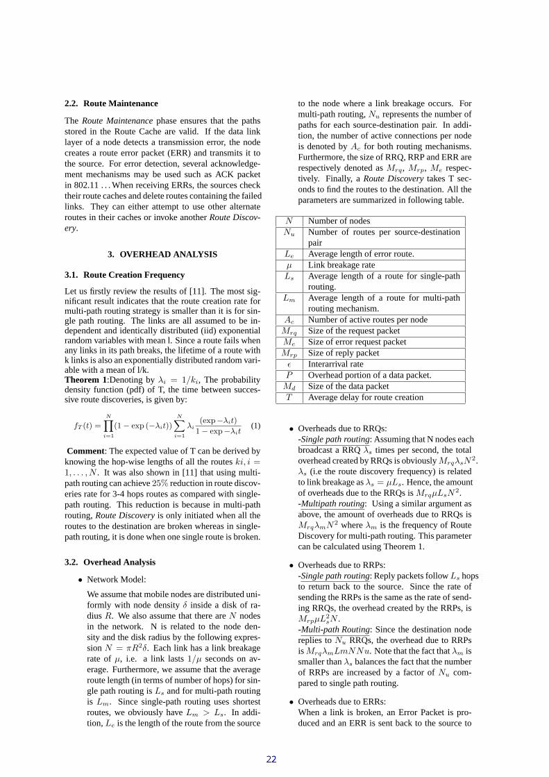
2.2. Route Maintenance

The Route Maintenance phase ensures that the pathsstored in the Route Cache are valid. If the data linklayer of a node detects a transmission error, the nodecreates a route error packet (ERR) and transmits it tothe source. For error detection, several acknowledge-ment mechanisms may be used such as ACK packetin 802.11 . . . When receiving ERRs, the sources checktheir route caches and delete routes containing the failedlinks. They can either attempt to use other alternateroutes in their caches or invoke another Route Discov-ery.

3. OVERHEAD ANALYSIS

3.1. Route Creation Frequency

Let us firstly review the results of [11]. The most sig-nificant result indicates that the route creation rate formulti-path routing strategy is smaller than it is for sin-gle path routing. The links are all assumed to be in-dependent and identically distributed (iid) exponentialrandom variables with mean l. Since a route fails whenany links in its path breaks, the lifetime of a route withk links is also an exponentially distributed random vari-able with a mean of l/k.Theorem 1:Denoting by λi = 1/ki, The probabilitydensity function (pdf) of T, the time between succes-sive route discoveries, is given by:

fT (t) =N∏

i=1

(1 − exp (−λit))N∑

i=1

λi(exp−λit)

1 − exp−λit(1)

Comment: The expected value of T can be derived byknowing the hop-wise lengths of all the routes ki, i =1, . . . , N . It was also shown in [11] that using multi-path routing can achieve 25% reduction in route discov-eries rate for 3-4 hops routes as compared with single-path routing. This reduction is because in multi-pathrouting, Route Discovery is only initiated when all theroutes to the destination are broken whereas in single-path routing, it is done when one single route is broken.

3.2. Overhead Analysis

• Network Model:

We assume that mobile nodes are distributed uni-formly with node density δ inside a disk of ra-dius R. We also assume that there are N nodesin the network. N is related to the node den-sity and the disk radius by the following expres-sion N = πR2δ. Each link has a link breakagerate of µ, i.e. a link lasts 1/µ seconds on av-erage. Furthermore, we assume that the averageroute length (in terms of number of hops) for sin-gle path routing is Ls and for multi-path routingis Lm. Since single-path routing uses shortestroutes, we obviously have Lm > Ls. In addi-tion, Le is the length of the route from the source

to the node where a link breakage occurs. Formulti-path routing, Nu represents the number ofpaths for each source-destination pair. In addi-tion, the number of active connections per nodeis denoted by Ac for both routing mechanisms.Furthermore, the size of RRQ, RRP and ERR arerespectively denoted as Mrq, Mrp, Me respec-tively. Finally, a Route Discovery takes T sec-onds to find the routes to the destination. All theparameters are summarized in following table.

N Number of nodesNu Number of routes per source-destination

pairLe Average length of error route.µ Link breakage rateLs Average length of a route for single-path

routing.Lm Average length of a route for multi-path

routing mechanism.Ac Number of active routes per nodeMrq Size of the request packetMe Size of error request packetMrp Size of reply packet

ε Interarrival rateP Overhead portion of a data packet.Md Size of the data packetT Average delay for route creation

• Overheads due to RRQs:-Single path routing: Assuming that N nodes eachbroadcast a RRQ λs times per second, the totaloverhead created by RRQs is obviously MrqλsN

2.λs (i.e the route discovery frequency) is relatedto link breakage as λs = µLs. Hence, the amountof overheads due to the RRQs is MrqµLsN

2.-Multipath routing: Using a similar argument asabove, the amount of overheads due to RRQs isMrqλmN2 where λm is the frequency of RouteDiscovery for multi-path routing. This parametercan be calculated using Theorem 1.

• Overheads due to RRPs:-Single path routing: Reply packets follow Ls hopsto return back to the source. Since the rate ofsending the RRPs is the same as the rate of send-ing RRQs, the overhead created by the RRPs, isMrpµL2

sN .-Multi-path Routing: Since the destination nodereplies to Nu RRQs, the overhead due to RRPsis MrqλmLmNNu. Note that the fact that λm issmaller than λs balances the fact that the numberof RRPs are increased by a factor of Nu com-pared to single path routing.

• Overheads due to ERRs:When a link is broken, an Error Packet is pro-duced and an ERR is sent back to the source to

signal the link breakage. Recall that Le is theaverage length of the path from the broken linkto the source (Le < Ls < Lm). Since the errorpacket has to travel Le links to the source, thiseffectively produces Le error packets per routebroken.-Single path routing: for each node, the breakagerate of the active routes is µAc . Therefore, ina N-node network, the average number of over-heads due to error packets is µLeAcNMe.-Multi-path Routing: In multi-path routing, sinceeach source-destination pair maintains Nu routes,the overheads due to error packets is NuµLeAcNMe.

• Overheads Due to Data Transmission:

The overheads created during data transmissionis due to the overhead portion of data packets.We assume that the each Route Discovery is ac-complished in T seconds on average. Further-more, each mobile node is a simple source withdata transmission rate of ε once the route discov-ery is completed.-Single-path Routing: Since the route discoveryrate is λs, the interval between each route dis-coveries is on average 1/λs. Each route discov-ery takes on average T seconds. Therefore, theactual time for data transmission is (1/λs − T )seconds. The number of data packets sent duringthat interval is (1/λs − T )ε. Thus, data packetsare sent with an average rate of λsε(1/λs − T )packets/sec. Since each data packet has to travelLs hops to the destination, the total amount ofoverhead is λsε(1/λs−T )PLs = µLsε(1/(µLs)−T )PLs-Multi-path Routing: Using a similar derivationas above, the total amount of overheads for mul-tipath routing is λmε(1/λm−T )PLm where λm

can be calculated using Theorem 1. (we do notinclude the derivation of this calculation in thispaper by lack of space).

• Summary:

The total amount of overheads due to RRQs, RRPs,ERRs and data packets for single path and mul-tipath respectively denoted by Ovs and Ovm canbe expressed as:

Ovs = MrqλsN2 + MrpλsLsN+ (2)

µLeAcNMe + µLsε(1/(λs − T )PLs

Ovm = MrqλmN2 + MrqλmNLmNu (3)

+ µLeAcNMeNu + µε(1/λm − T )PLm

In figure 1, we have plotted Ovs and Om asfunctions of the number of paths Nu. One cansee that there is no significant increase in over-heads for Nu up to 3. This confirms the fact thatin the literature, authors often mentioned that Nu =3 provides an optimum trade off. This claim isusually based on simulation results and the study

provided in this paper confirms this observation.In figure 2, Nu = 3 and Ovs and Ovm are com-pared as the link breakage is varied. It is interest-ing to note that the maximum increase in over-head ia approximately 20% (for a link breakagerate of 50%). Otherwise, for link breakages lessthan 10%, the increase in overhead is approxi-mately 10%. One might argue that the figure isnot insignificant. In fact, assessing whether thisincrease in overhead is acceptable or not reallydepends on the advantages brought out by multipath routing. This is why a theoretical study suchas the one proposed in the following is necessary.

4. TRAFFIC ANALYSIS OF SHORTEST PATHAND MULTI PATH LOAD BALANCING

ROUTING MECHANISMS

The following section compares the traffic distributionfor the shortest-path and load-balancing routing mech-anisms. We will be able to quantify the advantagesin terms of congestion avoidance of the load-balancingrouting mechanism over the shortest-path one. In par-ticular, we will be able to determine in which networksmulti-path routing really present interest. We will alsoderive an upper bound for a certain parameter whichwill guarantee that when multi-path routing is worthconsidering, it results in congestion decrease.

4.1. The Network Model

Nodes communicate with each other at a rate λ. Eachnode is assumed to have the same processing power ofη. There are two types of traffic going through eachnode, i.e. the common traffic which is defined as apoint-to-point communication traffic between nodes andthe relay traffic which is defined as the forwarding traf-fic caused by data packets travelling through multiplehops to the destination.

4.2. Analysis of The Shortest Path Routing Algo-rithm

It can be found in [15] that the total traffic going througha node located at a distance r from the center of thedisk, λ(r) can be expressed as follows:

λ(r) = (πR2δ − 1)λ +π(R2 − r2)2δ2λβ

2(4)

Therefore, according to Little theorem, the average num-ber of packets in the queue for a node located at a dis-tance r from the center of the disk is:

Npac(r) =λ(r)

η − λ(r)(5)

Further, the average number of packets in the queue forthe whole network can be evaluated as:

Npacs =∫ R

0

2πrδNpac(r)dr (6)

The exact calculation of Npacs presents little interestin this paper since we are only interested in a generaldiscussion on the congestion avoidance. However, itis important for the following to know that Npacs

canbe exactly evaluated. Its expression can be found in[15]. This parameter is a good indicator of the generalcongestion of the network.

4.3. Analysis of the Multi-path Load Balancing Rout-ing Mechanism

A perfect load balancing multi-path mechanism dis-tributes the traffic evenly among nodes in the network.As a consequence, “hot-spots” are eliminated. There-fore, packets are expected to experience lower averageend-to-end delay. Suppose that Lm, λm and η are re-spectively the average length of a route in a network,thenode to node traffic rate, and the processing rate. Let usevaluate the total traffic within the network. Since thenumber of nodes is πR2δ, it is easy to see that the to-tal number of possible connections within the networkis (πR2δ − 1)πR2δ. With an average route length be-tween two nodes of La the total traffic within the net-work is (πR2δ − 1)πR2δλmLm. Therefore, the in-coming traffic per node is (πR2δ − 1)λmLm and theaverage number of packets in the queue per node is:

Npacm=

(πR2δ − 1)λmLm

η − πR2δ − 1)λmLm(7)

In order to ensure that the load balancing policy de-creases the congestion level of the network, Npacm shouldbe smaller than Npacs . One can see in the above equa-tion that the key parameter which controls Npacm

isthe average length of a route. Indeed, in order to haveNpacm

< Npacs, Lm must satisfy:

Lm <Npacs

η

(Npacs + 1)(πR2δ − 1)λm= Lmax (8)

This result shows that if Lm > Lmax, using a loadbalancing routing mechanism is no longer beneficial ascompared with a shortest-path routing scheme. Thiscan be easily implemented in practice: given a networkcharacterized by its node density, its size and the trafficrate, one can evaluate Npacs . This value can then beused to calculate the theoretical value for Lmax whichis interesting for two reasons:

• First, if Lmax is smaller than the average routelength for single path routing Le, then obviously,this means that there is nothing to be gained byusing a load balancing policy.

• Second, assuming that Lmax > Le, the resultof this section can be used to select routes thatrespect Lm < Lmax.

In the next section, we will investigate another issueassociated with a load balancing routing mechanism,namely the connection throughput of the network.

5. CONNECTION THROUGHPUT ANALYSIS

In this section, we compare how the resources for trans-mission are used within the network for single path andmulti path routing.In order to conduct this study, we de-fine the concept of connection throughput as follows:The connection throughput of a network is the aver-age transmission rate of a connection in the network.Note that the connection throughput is a good indicatorof the average end to end delay in the network. Intu-itively, we can see that congestion restricts the full us-age of the available bandwidth. In other words, assum-ing that every route can support in theory a transmis-sion at W bits/seconds, the actual transmission rate of aroute is limited by the fact that the bandwidth has to beshared with other routes at the MAC layer of each node.Therefore, the transmission rate of a route will be lim-ited by the bandwidth available at the most congestednode of this route. A load balancing policy which re-lieves hot spot congestion should improve the connec-tion throughput of the network. However, one has to becautious since while the transmission rate in hot spotareas increases due to congestion avoidance, it also de-creases elsewhere in the network where more traffic isdistributed. There is therefore a trade off to considerwhen applying multi path routing. An interesting pa-rameter characterizing the performance of multi-pathrouting is the average route length (calculated in num-ber of hops); When this parameter increases, it resultsin more nodes in the network involved in connectionwhich means that more traffic is distributed across thenetwork. In the following, we propose an upper boundon the average length of a route in multi-path routing,which guarantees that the connection throughput is in-creased as compared to single path routing.

5.1. Single path routing

In this section, we use the same network model as insection 4. According to (4), when a single-path rout-ing mechanism is used, nodes closer to the disk centerare experiencing more traffic, i.e. are more congested.Therefore, in terms of capacity, the total capacity of thenetwork is limited by the capacity of the area close tothe disk center. Consider a node A with distance r fromthe disk center with radius R in Fig 3. Consider a con-nection between nodes A1 and A2. We will assume thatthe route between two nodes can be approximated by astraight line. We will later on discuss the limitation ofthis approximation. Let us denote by A, the orthogonalprojection of the disk center O on the line A1A2. As-sume that there is a node on the route between A1 andA2 very close to A. This is a valid assumption since wedeal here with congested networks for which the nodedensity is generally high. We will refer to this node asA for sake of simplicity. Since this particular node iscloser to the disk center than any other nodes on theroute, it experiences the highest traffic of route. There-fore the data transmission rate on this particular routeis limited by the congestion experienced by node A.It can be easily seen from (4) that the number of routes

going through node A can be expressed as:

n(r) = (πR2δ − 1) +π(R2 − r2)2δ2β

2(9)

Assuming that we have a fair MAC layer, each routeis allocated an equal bandwidth for data transmission.Therefore, each route going through node A will be al-located the bandwidth denoted by W (r) expressed as:

W (r) =W

(πR2δ − 1) + π(R2−r2)2δ2β2

(10)

where W is the total bandwidth allocated to the net-work. It can be recalled that πR2δ is equal to N , thetotal number of nodes in the network. Assuming thisnumber is large, then we will assume in the followingthat πR2δ = N .Let us now evaluate the number of routes which trans-mission rate is limited by node A. Note that theseroutes have to be perpendicular to OA and go throughA. One can see in figure 3 that these routes are suchas their source and destination nodes are respectivelyin the areas R1 and R2 and vice versa. The number ofnodes in each area can be expressed as:

NR1(r) = NR2(r) = (R2 − r2)βδ (11)

The derivation which leads to this results is very sim-ilar to the one leading to (4). We will therefore re-fer our reader to [15] for more details. From this, thenumber of routes which transmission rates are limitedby W (r) is simply 2NR1(r)NR2(r). Note that anynode in the ring delimited by r and r + dr with drsmall enough will have the same traffic characteristicsas A(r). Therefore, it can be shown that Csp, the totalbandwidth used by the network will be expressed as:

Wsp =

∫ R

0

W (r)2NR1(r)NR2(r)2πrδdr (12)

= 2Wδ

∫ R

0

(R2 − r2)2β2δ2

(πR2δ − 1) + π(R2−r2)2δ2β2

2πrdr

= 2W

√βN

2π(

√βN

2π− arctan

√Nβ

2π)

Note that we have used the fact t that πR2δ = N .The total number of possible connections being N2, theconnection throughput for this network using a singlerouting mechanism is λsp = Wsp/N

2

5.2. Multi-path Load Balancing Routing

Suppose that and Ac is the average number of activeroutes per node. Obviously, the number of active routesin the network is NAc. Lm being the average numberof nodes involved in a route, the total number of con-nections in the whole network is NAcLm which meansthat the number of connections per node is AcLm. As-suming that the bandwidth available at each node isuniformly split among these connections, the bandwidthper per connection is W/(AcLm). Therefore, the totalbandwidth used by this network is:

Wmp = Number of active routes × connection bandwidth

= NAcW/AcLm = NW/Lm (13)

The connection throughput is λmp = Wmp/N2.

This result shows that the capacity of the network isinversely proportional to the length of a route. Thisconfirms our initial comment that increasing the routelength means distributing more traffic across the net-work, therefore decreasing the average connection through-put. It is therefore useful to compute an upper boundon Lm which allows ensuring that

λmp > λsp (14)

This leads to:

Lm < L′max =

1

2( β2π

−√

β2πN

arctan (√

βN2π

(15)

It is worth noticing that Lmax is itself bounded as fol-lows:

Lmax >π

β(16)

Remember that β is a constant characterizing the factthat routes between source and destination nodes arenot perfect straight lines. This parameter which onlydepends on the network density can be evaluated bysimulations for instance. When the network density ishigh, β is typically small. Therefore, Lmax will bea large number. For instance, for a network consist-ing of 100 nodes in 1 kilometer square, β ≈ π/16.We therefore have Lmax > 16. However, on average,simulations show that the average path length in multi-path routing is around 6 or 7 hops. This means thatthere is in fact no constraint on Lm as far as connectionthroughput improvement guarantee is concerned. Inother words, using multi-path routing always improvethe connection throughput of the network as comparedto single path routing.

6. CONCLUSION

In this paper, we have analyzed and compared singlepath and multi-path routing algorithms. We have firstconcentrated this study on the issue of overheads, in-herent to multi-path routing. We have shown how theamount of overheads increases with the number of mul-tipaths and we have seen that when this number ex-ceeds three, the overheads increase dramatically. Thishas confirmed many simulations results presented inthe literature which state without any clear explanationthat using three paths provides the best trade off. Wehave also derived an upper bound on the average lengthof the multi-path routes which guarantees a decrease ofthe network congestion. This upper bound depends onthe traffic intensity, the processing power of each nodeand the number of nodes in the network, hence is easyto compute in practice. Not only this bound allows toselect routes that respect the upper bound constraint,but also, it can indicate in the first place whether fora particular network, using load balancing will bringany improvement at all. Finally, we have shown thatusing multi-path routing always results in connectionthroughput improvement for dense networks.

Fig. 1. Overhead comparison when Nu increases

Fig. 2. Overhead comparison as the link breakage rateincreases

Fig. 3. Network model for connection throughput

7. REFERENCES

[1] N.F. Maxemchuck, “Diversity routing,” in IEEEICC’75, San Francisco, CA, June 1975, IEEE,vol. 1, pp. 10–41.

[2] R. Krishan and J.A Silvester, “Choice of al-location granilarity in multi-path source routingschemes,” in IEEE INFOCOMM’93. IEEE, 1993,vol. 1, pp. 322–29.

[3] R.Rom I. Cidon and Y. Shavitt, “Analysis of

multi-path routing,” IEEE/ACM Transactions onNetworking, vol. 7(6), pp. 885–896, 1999.

[4] R.C. Ogier and V. Ruthenburg, “Minimum-expected-delay alternate routing,” in INFO-COMM, Florence, Italy, 6-May 1992, pp. 617–625.

[5] Nageswara S. V. Rao and S.G. Batsell, “Qos rout-ing via multiple paths using bandwidth reserva-tion,” in INFOCOM (1), 1998, pp. 11–18.

[6] S.J. Lee and M. Gerla, “Aodv-br: Backup routingin ad hoc network,” in IEEE WCNC 2000. IEEE,2000, pp. 1311–16.

[7] L. Wang et al, “Multipath source routing in wire-less ad hoc network,” in Canadian Conf. Elec.Comp. Eng., 2000, vol. 1, pp. 479–83.

[8] S.J. Lee and M. Gerla, “Split multi-path rout-ing with maximally disjoint paths in ad hoc net-works,” in ICC’01, 2001.

[9] M.R. Pearlman et al, “On the impact of alternatepath routing for load balancing in mobile ad hocnetwork,” in MobiHOC, 2000, p. 150.

[10] A. Tsirigos and Z. J. Haas, “Multi-pathrouting in the presence of frequent topologi-cal changes,” IEEE Communications Magazine,November 2001.

[11] A. Nasipuri and S.R. Das, “On-demand multi-path routing for mobile ad hoc networks,” in IEEEICCCN’99, 1999, pp. 64–70.

[12] D. Johnson and D. Maltz, “Dynamic souce rout-ing in ad hoc wireless networks,” in MobileComp..., T. Imielinkski and H. Korth, Eds. 1996,Kluwer.

[13] C. Perkins and E.M. Royer, “Ad-hoc on-demanddistance vector routing,” in IEEE Workshopon Mobile Computing Systems and Applications(WMCSA), 1999, pp. 90–100.

[14] V. D. Park and M. Scott Corson, “Temporally-ordered routing algorithm (tora) version 1: Func-tional specification.,” Internet-Draft draft-ietf-manet-tora-spec-00.txt, November 1997.

[15] P. Pham, “Proofs for witsp2002,”http://www.itr.unisa.edu.au/ ppham/witsp2002/proof.pdf,2002.

"!#$%&'()+*,$!*)( -.( /0),+1234!)5+

687:9<;>=@? AB=@C:DFE8?E8?:GHIE87:JLKNMO7:9<;>PQE8GRLPJ@PSMOD(D/7:?:=@SQET;>=@MO?:9&E8?:GUV?XWYMOZ[DFET;>=@MO?RLPS\:?:MOJ@MO]8^_`P9[PQE8Z[S\ UV?:9<;>=a;>7X;>P

bc?:=adOPZ[9[=a;V^)M8WLefMOJ@J@MO?:]OMO?:]:gXh$ijeglkm7:9<;>Z>E8J@=nEo[p 7:9<;>=@?g:ClE87:Jrq8sm;>=a;>Zt 7:Mvut PG:7t E87

68MO\:?w687:G:]OPxM8;>MOZ[MOJnE/km7:9<;>Z>E8J@=nE8?_`P9[PQE8Z[S\+yNP?z;>Z[P| ABMOZ[Gwij;>Z[PP;Qg~KNM8;E8?z^Og~h$ijeglkm7:9<;>Z>E8J@=nE

p MO\:?t p 7:G:]OPvs$D(M8;>MOZ[MOJnEXt SMOD

c&jc`#l` <mT< v& )vr<' T

c '8r mY'&T<'<[ QT¡v ¢T£¡vLv¤T¡ j¥z¦§B' ~£¨vYO O¨© v& /vr<' T ª«Qv[ª¨T < <$¥F¬¨'T8<' vv¡T['vY ¡v[T#­TQvv '[¨Tr®' vr& vr<' T / ' cª¨v&Yv¨Tm¯Q<T`#¡ 8 $<>°­TQvv T¥f±B Y°Tr[ª²¡ 8 #³B<>°­TQvv ´a±L²µ¶³L·I¡Tr[©¡v Y°nTr[c¨&'«QvIN<<¢'[¨vr.$v<' ¨/v[r Y°< ¨v8 $vv[ Q¡ m­TQvz¥$±L²µ¶³¸&>°8¡Tr[ 'L¨<<<¡T¹<Q«Q '<XB¨<¨v L¡v Y°lL¡TV '88¨N«°Q £v«QB¨TV<Y<´Tr<°8<[ T·V ¡Tr<~v¤T[/¨TV<Y<'´8<<« <T>·£Tª< ¨Q8rTr[¡v [<¥£¦§¨IT8<[ O#¯' ¨Nº[VB: ' &'v<«Q» Tr<°`8<c­TQvQ T¥½¼ª/r¨¾¨T$'T[F( T)­TQvv T'#¡ 8 <>°­TQvv T Q±L²µ¶³«Qv[~>«<B '«<'< c¨£Q¡#8<:' [<YXz¿ÀÁ «<~²µ¶³T [Âà Á «<: T­TQvv T¥

Ä8ÅÆÇ `È&ÉmÊ# Æ È ÇË ' $¨vcY´a² ËLÌ ¶¬¢·' [V 'OB < [:' Bvv[:' ©I<'8°Y`Q N¨#< Í<[mv' Y $YTr¡8r$r<«Q[&<¡ °F>«

Q«< T~Yv<¥ Ì vv[N F² ËLÌ ¶¬ÎVX¡v<< [v LT<¥X² ËLÌ ¶¬BX&>°©¡vv<[Ï¡<B¨T[¶ c¨< ¨Q°vr<T8 °¥² $vv['&>°'«¨T ¨< `Y v< (T Y¡T<¥ Ì <-vv[N&>°/¡¯Q8[V[v °cÐY ¨`Y¯vY vv[&>°¡¯v8[V[v °/ [>« ¹'«&¡vNB&#rB ¨Ñ:¥:µ:r TX8¨¢Y©&>°¯v8< <TBTr N'< T QB¨¨cv§v<' Y¥ ˲ ËLÌ ¶¬&>°N8<¢ `r &[V[NB¤¯v[Y&´¦§<V·j«QI¢TrY m´>°·V¥ Ë ² ËLÌ ¶¬Ò<8/¨TV< Í<[Q°) TTvBQ¨j T¨ ¨$<B[< v <' r<I[V «Q Y°f´Tr Q·V © ' [ Tr'r Tmv<«Q©8<BTY <¥

¦§'² ËLÌ ¶¬£ v¨£zX v& $vr<N T &~&¯v ' Í<B¨I>« Y°#¹² ËLÌ ¶¬< v& -´º8 <ªv<«QF¨TrV<Y<·N< ¨<c v< °(` T °¨¡¨¡v¨² ËLÌ ¶¬ÓB¨ T¡ ' &I'#¡ < TNT(v<«Qm«<¨[<¥ÔI «<¨$T¡I/² ËLÌ ¶¬£ X¨'8r['ª¨T < ª <$¥Ë Q°( v& vr<' T F'[¨Tr#¡TYTT#8¨¨'[Ï¡ <'<I~¨& < T¨TY `#8¨¨/v<«Q/T)¨² ËLÌ ¶¬£¥jÕ¶TY B¨TI<[$c8NTrv<[ÖO8<[ ['¡v ©T£'#¡< T<¥¹l¯Q[r «`'¡v v¡&' <[ª­TQvv '[¨Tr&< £¡[<[°)¡ #8<<Y< [<v T)v[r ¡[<[°(T

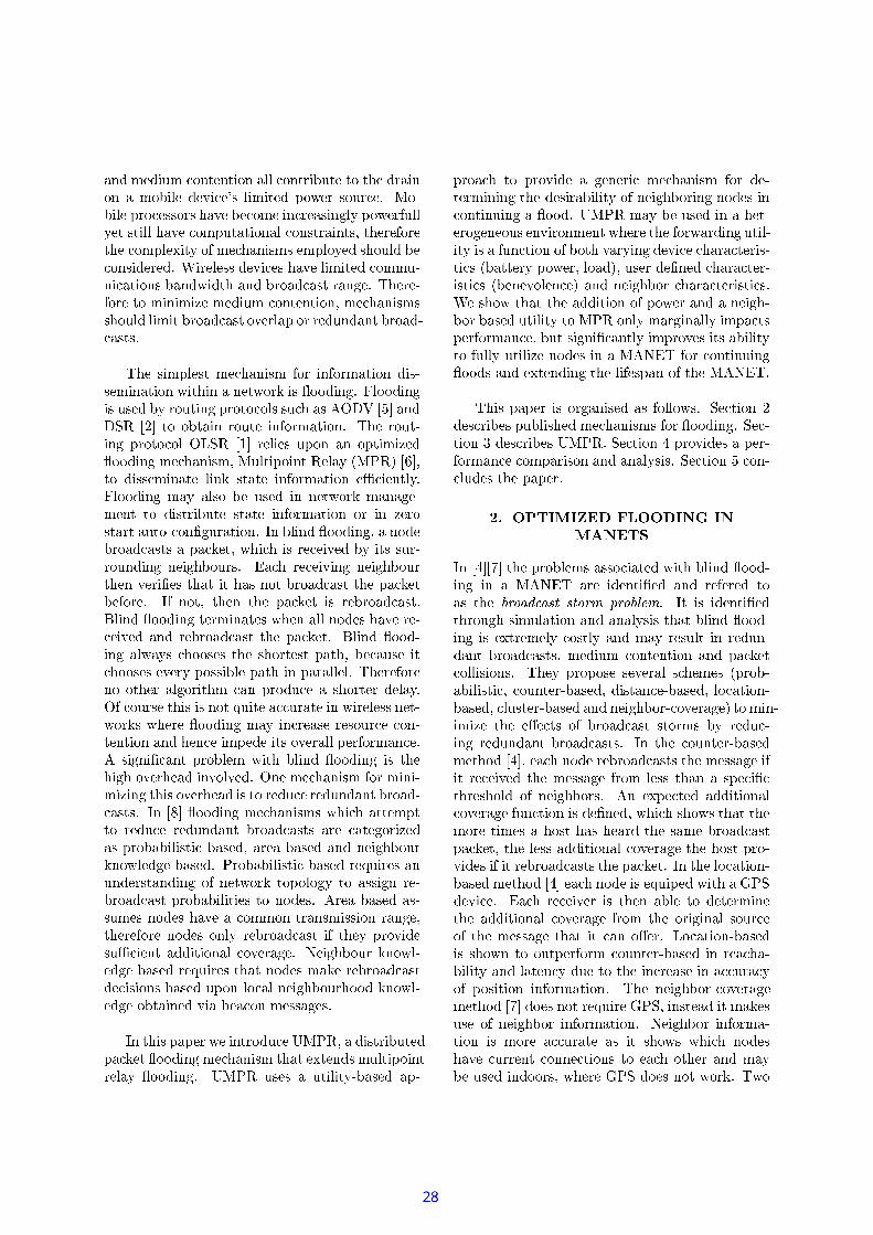
Ã

T'[v ¡f< ' v ¡vI¨Bv F' $v<«Q» N ' [F8<'r¡¥(² v[rz¨T>«¶8['¶ T[r °£8<r¡ °Y O¨T>«¢'¡v TOTY < ¨<¨' ¯v Y°£T'[¨Tr&X<' °[r¨¡©8Trv<[z¥¹¼) < [lv<«Q[l¨T>« ' [&'#¡v< T~TTvBQ¨mT&<Y¶¥:¬¨<LN' ' Í<£'[v ¡Ó< j v'[¨Tr&r¨¡I ' ¹<YO«<Iz[v¡TjQ<Y<¥¬¨$r ' [Y&'[¨Tr®' v& (vY

r<' T NB ¨ `£Y©:­TQvv T¥X Qvv X¡Tr[Q°©¡v IvXr¡T¨N Ë ÀT ³ à ªv ¡vc v& j¥/¬¨m¡vr /v ³ L< ['¡8)v ' Í<[­TQvv ©'[¨Tr$ ²¡ 8 ³B<>°m´a²µ¶³L· ¿n Fvr<' Tª Yª v& ` < °¥X Qvv &>°r/8¡Tr[ )Y&T'<$vY ¡vY/ v& wÍ<<Yrl¡v§v¤T¡ j¥j¦§N T#­TQvv T Ivv<Y¢`T[ TB¨¨I[< «[$Q°m £r¡r¡Tv < ¨Q8¡<¥f¶¨[< «Q < ¨Q8¡¨<«< ¤T[¨TI I¨T¢L<YB¨#T8¥ ¦n'[ I¨<w¨T$<<Y[¥ T&­TQvv <' T[¶B¨<m Ovv[¶¨T>«L< «[T<<Y¨mT[¥ T­TQvQ ª >°v#¨Qr[©¨$r¨r[YNT¨j l8[<¡Trc ¨Qr[<«<°&8r £T¨$ $T <@¥l¬¨<¨<& ¨ <vv¡T$ªr¨r<'v<>°¥ 8¡r~¨XX~Ï¡ <¡¶ NB < [¹rvIB¨<N­TQvv $&>° T[r'[r¡'v< `T'¨<T¢ '8[vL ~«< v8<r&T¥Ë r ¤8<& <B ¨ T(­TQvv /'¨¨ ¨&«<¨[N Q« «[z¥ L'[¨Tr½' ' Í< ¨j«<¨[¢OB[v¡Tl[v¡TjQ<Y<¥¦§ l­TQvv m'[¨Tr&IB¨¨/r<'v[v¡T/[v¡T<Y$<< Í<[IT YNTr[z ¹[cTr[ªTª< ¨Q8¡QB [v©Tr[z¥¢µ~T Y£Tr[$[Ï¡ [¢¡Tv<YTv ªLYª8 °//r (<YIT [Ivv[<¥ Ë [mTr[ªYr¡'[Lvv[I¨T>«Nm''Tr'r ¨<cvv[N °<<Y# L¨<°«Qvr¡v` <'v T«<¥ Ì < ¨Q8¡#QB [vTr[$[Ï¡ [¨TIvv[¢&<<Yv[r TTr[m¡8 v<j< ¨Q8¡¨QvcQB [v£v [c«QN8[m'[[<¥¦§£¨zT8<jl vv¡T~±L²µ¶³© [BvY ¡v[

TO­TQvv B'[¨Tr¨Tj¯Q<Tj#¡ 8 <>°F­TQvv T¥ ±L²µ¶³ ¡Tr[F¡v Y°nTr[ v

¨«Qv<</'[¨Tr v<' #¨v[r Y°'X< ¨Q8 #vv[ Q¡ &N­TQvz¥¶±L²µ¶³ &>°c8©¡Tr[m '¨r<<<¡T8<Q«Q '<zB¨<:¨lv ¡v Y°IX¡TV #v8¨#«°Q ¢v<«Q¨TV<Y<£´Tr<°&8<[ T·V Q¡Tr<Bv¤T[m¨TV<rY<`´8<<« <T>·£T< ¨Q8¨TV<Y<<¥¼ª#r¨¨T¢¨#v $:8<¢T'< ¨v8lTr[#¡v Y°²µ¶³( °& T °© 'TV8<r&T ¡vBr ¤8< °N '«[l Y°'¡ °m¡v Í<vv[B '² ËLÌ ¶¬L Q¡ ­TQvT`¯Q<Tv #¨I [rTcj¨©² ËLÌ ¶¬£¥¬¨T8<r[ª£ ¢<¥ [V Ã

v[ 8[l¡ r¨[''[¨Tr&Xl­TQvv T¥ [V  v[ 8[±L²µ¶³©¥ [V N«Qv[N8<r&T¢'Tr'T&T °vr<¥ [V cÀ©v ¡Tv[¨©T8<[¥

zÅ È© Æ Æ É !ÈcÈ&É ÆÇ#" ÆÇ Ç$ N

¦§ % 8¨I <&rv['B ¨c T`­TQvQ ½² ËLÌ ¶¬ v< ¤T[ Tw<[ &¨'&(*)+-,-./+02130214)(25768(*)-&9 :5N¥ ¦nmcv< ¤T[¨¡¨$r #¡ T$T °vr¨TL Tm­TQvQ ¯Q<'< °Y °ªT/&>°[r¡ [v¡v&<Y< ~'[v ¡.< FT(T r T<¥¬¨<°(8rr<«<B¨<'[´v Y ¹¡<rnTr[z jvYTnTr[z z v< vTr[z > ¡TY<rnTr[ITI< ¨Q8r§«<>·B' v ' Í<ª¨/ÑO[V$N<Y$Y&mQ°[v¡TV /[v¡T'<Y<¥¦§F¨¡<rnTr['¨v ;n [¨'vv¢<<YX¨¢'[B N[< «[ª¨c'[&® [¨T(r8[ ¤8¨[r¨©< ¨Q8<¥ Ë ¯v8[V[v T«<~¡TV &¶v¤T[z B¨¨`r¨¢X¨T~¨'# '[©m¨Y£¨T£¨[¨&''<YT[ T¨# [Lv T:«<I¨#¨YI«Qv[¹ T X<<YO¨T[¥j¦§©¨ v< vTr[©'¨v [¨vvX[Ï¡ 8[B ¨'IÔ£µ v<«Q¥¶¨([< «<''¨<) $v<' ¨v T¢«<& ¨ TBr¡¨`'[N¨T# '</ÑO<[¥ v< vnTr[#r¨Bª¡v8<r®¡<rnTr[ [¨T Y°mTc<T°cv¡£'¨© T[rI <¡°#8r v& j¥Ó¬¨/< ¨Q8r§«<'¨v % TvQ[Xl[Ï¡ BÔ£µ > TY[# l&[¡Tr$I< ¨Q8& v& j¥ Ì < ¨Q8' v& +'<¡ /r¨¢B¨¨+vv[¨T>«`¡<N[V T©[¨¨<NT/&>°8¡Tr[$ TvQ< B¨<#Ô£µ vQ[¢¢O¥¬

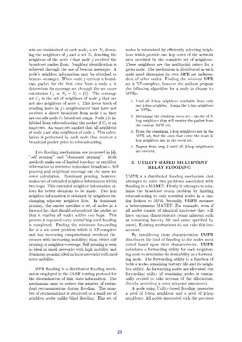
Â

rI& [cB[¨cvv Nr£v<r m¨`< ¨Q8I£T/rBv< $¨< ¨Q8©¨cvv:¨TNvv©[< «[ª¨<YBT¢$¥ Ì < ¨Q8Lv< ¤8< ¨ <«[$¨¡¨¨'¡Tr'8[ª'[[<¥ Ëvv» < ¨Q8 v& &>°ª8mr¨[ª8['[[<¥L¼)¨<vv¢[< «[L`Q<YmTcc¨¤TYm ' vvº L v<' [L £«<rL¨¡¨¨'r©«<<¡ ¥ ¬¨«<r m©¨$r#¢< ¨Q8¢vv©¨T'£rc< ¨Q8L~vvº¥¬¨I<<T¢$8<Tv ¨Y V» #< ¨Q8¨Qv¨TN¨T>«&[< «[(v [V&<Y'vv '¨<°B¡vrv¢vvº» ¶<Y~¥ Ì vv!l~ v¨ [&Î<<Y £¨IT I<'vY°vr[¥ Ë m<'vY°vr ' [¶¨TB O< ¨Q8¹vv¶Ir#< ¨Q8¶¹vvº¥~¬¨<¡v /8<r'[ªQ°ª[¨/vv&¨T#[< «[©<YTB &<<Y T¥¬'­TQvv &'[¨Tr&¢©8r[c  n

" r< &¡ " T " v' T¡ " ¥ ¨'¨vl&¡TrBO ' [#8 °l< ¨Q8 v& L¢' ' Í<l[v¡Tj<Y<¥ < ¡ `Tm< ¨Q8¡¢«<I¡Tr£¨#'r«<$<¡ j¥ ' T¡ T £¨<«<[ &[O¡TrlQ¯Q<Tv[£< ¨Q8z v& £B ¨ Y¨T<¥:¬¨¶¯Q<Tv[&< ¨Q8¶ v& c ¢N&8r<cv[r TN8&v¥¬/¨< ¨Q8~ v& &~v ['Q°N< ¨Q8l¯Q¨T >Ðr<ª< ¨Q8 Y<¥ ¦§½v' T¡ T :¨$r<Tv<'r8[ ¤T['rNLvv[# FN Y¶¨Tr¨¡&<<Yl¨ITr¨T& &[¨[N vv['B ¨ (Yª¨T<¥F¬¨v[j¹<8[[£<«<°£r[T©¨¡ ­TQvv &' [z¥ X Tv /¨' #¡ v YrN«<£ < B¨¨/ Ì µl§' T¨T$ T[r F'¡v T£«<¨[ ´ v[r[IB ¨ T[r m' Y°·I¨T/< ¨<#r< ¡ Il< ¨Q8r§«<¥ < O¡ £lr<<v[z r& OYvB ¨$¨ ¨m' Y°cTv' Tj¡ Bv[ £:YvOB ¨©'vQ<I' Y°¥²µ¶³+­TQvv m£cvY ¡v[­TQvv c'[¨v

rf<' °[' &¨ ³)¡v vv¨`vr<' T ª /Y' v& j¥c¬¨'[¨Tr &I$[v¡TN¨&Q¡#8<©[v¡v#Tr'r Tv¡ ­TQvv T¥¬¨cQ¡N8<¶jTr' r<~¶[YV[NNr& Or< ¨Q8Lvv[I¡ # T­TQvv T¥©¬¨Ir£

vv[£©' ' Í<[ªQ°` < °ªr< [V $< ¨v8LB¨¨«Qv##¨ª«<Ll¨'Y[«Qv[(Q°¨' r`I< ¨Q8<¥¬¨[r< ¨Q8c¨#¡ 8 $<>°v'$ «<'vv¥l¬¨¢'[¨Trf¶vY ¡v[&~[¨vvc#¡TYNv<' c #B²µ¶³-rN Tv<8<vv<NB¨<#vv[<¥#X Tv ¨c' &²µ¶³r£ Ì µl§' z¨<«<B¨&¡v¨¢8r¨m B / ¨®`vvm/¨Qrm ²µ¶³¢<Ö#$&%(' )+*-,/. .103254768 )79:' ;4=<>6/?A@?A93,/BC4+,/<7. 9ED ?A6FG6)7. H6)79&#2547681)79:' ;4=<>6/?3$JI!@K@K' ;)1LA479M#2547681)79:' ;4=<>6/?A@,/@MNOQP!@:$

0R$MSM9LA9?AFT' )79ULA479!?A9:@KV7. LC,/)RLB:6XWY9?@K9L2ZLA479!@K9L6/DQ0324768)79:' ;4=<>6/?A@LA4+,XL[U' . .\?A9:B:9:' WY9MLA479M8+,/BC]Y9LD ?A6FLA479&B:V^?K?A9:)RLNOQP@K9L3$

_=$&%^?A6F`LA479?A9:F,/' )7' )7;#254768)79:' ;4=<>6/?A@U)76/L!' )LA479NOQPa@K9L3b\c+)+*LA47916)79:@MLA4+,XLB:6XWY9?MLA4791FT6@dL0324768)79:' ;4=<>6/?A@U)76/LU' )LA479MB:6XWY9?!@K9L3$

e $MP!9:8>93,XL1D ?A6Ff@dLA9:8g0V7)RLA' .,/. .!03254768)79:' ;4=<>6V^?A@,X?A9B:6XWY9?A93*h$

ijÅ Êm Æ ! Æ TjlkN$ É Ê!O Æ #È ÆÇ !¶1j !ÈcÈ&É ÆÇ#"

±L²µ¶³¸vY ¡v[ª­TQvv '[¨TrÒ¨Tr<'v&Fr «$Y <&crv[FB ¨­TQvv `² ËLÌ ¶¬£¥ X Y °N r<'vl' v ' Í<¨(<YY" <"Q° ' <<Y / °[r<Bvv[' )/r N `ar¨ )(²µ¶³©¥ [Tv ° L±L²µ¶³Òr¡'[(¨<<<¡Tm² ËLÌ ¶¬£¥ $¯' L<«< Bvv['TrY&Iv<<B¨Tv`¨<°B ¨T>«`«°Q ª¨TV<Y<`´ar'c ¨<<'r¡T¨`<& Tr<°F ªT)r'ªr8[ ¤T[Q°¡Tr<·V¥ll¯vY #'[¨Tr&vN¢¨ <¡[¥°wTrv< ¨[rF¨TV<Y<< ©±L²µ¶³

vY ¡v[¨£ `¹­TQvv N#¨©vv['Yr¡ [Tr[F¡8)¨< m¨TV<Y<<¥±L²µ¶³<¡[£cv c¡v Y°£[¨ª< ¨Q8r Lvv¶£v<' :v[r Y°©XBQ $vv¥'¬¨Nv c¡v Y°©c¡TV ª8¨cvv[¶<& #Tr<°N £T& < ¨v8l¡v Y°¥ Ë Xv Ivv[lB v<[z ¨v ¡v Y°)#<& (vv[m$ v¡T °(<«Qr[(/<¡&£¨ v< T< ¨<<Q°`«Qv 'N'©<¡£r[r'<[¥Ë vv#¡Tr m±B Y°nTr[m­TQvv c<<[

(8Q© n¨< ¨Q8$T (8Q© Ã n¨< ¨Q8<¥ Ë Ovv[rv['B ¨`¨I<«Q ¡T

<Y&T(v ª Ym$<'«[¨ª8Q<¥ n¨< ¨Q8`B ¨ vY TV à n¨< ¨Q8Nm<'«[/ ¨ n¨8Q¢Tv[¨cv Y[¥(¬¨< '< ¨Q8 vv[£#<'«[$ ¨ à n¨8Q@¥#¬¨'& n¨(< ¨Q8NB ¨vn¡Ï¡ à n¨vv[:r [¢v L¡v Y°¥ Ë ' v< `¨<cv<¡< QB¨¨m¶¨ n¨`vvIB ¨¨c¨ ¨[YN¡v Y°ª¨cv Y'T'«[: à n¨'< ¨Q8:½¨¢8Q@¥l¬¨Brv £¡v Y°#l¨¢<& ©vv[~:¨<`«Qr[z v¨Q¡TQ &<¡BX¨# v< j¥~¬¨ Q¡[©¡ ¶¨`8Q#<'vY°/r[ X¨c& n¨©vv[¹lXv[IB¨~Q ( Ym¨< ¨ F¨< <Q<Y T¥l¬¨Iv N¡v Y°cBv¤T[$<Ö

B¨< T ! " $#%'&()* +,&(-)/.0 1 1" " $#%'&()* +,&(-)/.0

Nr8[ ¤T[¶¨£<& N <TO8<¡v Y°IBv<«Q¥ Ë r 'L¡TV #jr<<© ©¤T¡ L¡Tr[mcv<' ¨¡v Y°¢ L«Qv[¢Qv[Y &Nl¨'[Ï¡ [8<¨T>«Q N´ ¡v Y°/Tr ΨTcN ¸8<32~r¨T¨T ¡v Y°L'[v ¡ 8<32T¨ ¨¡v Y°Tr ¨TIB¨ ¨m8<V·V¥54 lr8[ ¤T[¨£<& <TT8<¶T&©« ¡¢76¥ 6£ 6¥ 6&´16¥ 68< ªv< [(T 6¥ 68< ¡ 8<V·©T 0£v¤T[I¨T ~¨N#~¨' <TX8<4 Y ~~ °¡Tr[Nr¨ º~¨¢r '#¡TV `Vv °¥¹¬¨8£¡v Y°©X[Ï¡TL¨Q¡#8<X¡T v<[< ¨Q8L n¨ªvv z¨T#`< ¨Q8NI¨<Y ªvvT ¨#8Q¹ à n¨< ¨Q8¢v «Qv[Q°c¨jQ¡#8<¢l v<z< ¨Q8¨ n¨$vv¥¬¨:[r¡ : 'Ivv» Xv I¡v Y°Nv[[Y IB¨<#<«Qr[T©[X<¡: à n¨vv[B¨¨&>°$¨T>«# [v°c8<<ª v<[z¥L²µ¶³+ 'Tr# °NTrv<X¨TvY TV à n¨< ¨Q8<¥¦§±L²µ¶³ª~r¡':¨: B TÖ Ì vv[z& v

' Y¢l< ¨Q8 'vv[< B¨¨mL'vv:¶v<[&Q°´ 9Q·V¥ [''[[lBQ<Y'8< vv< °/ª v< ¨Q8 vv['¨< j¯vYT¥ Ì < ¨Q8z v& ©r¡T¨©z8<T )r¨[8['[[<¥-¬¨m Y£¶vv[L[r8Tr £ Q¡ m

0

0.2

0.4

0.6

0.8

1

0 2 4 6 8 10

Util

ity

Power

Power Utility

power

X ¡ Ö~µ:<±B Y°:

Uf=0.095

E

D

Uf=0.73

Up=0.19Un=0.5

CP=3

A

I

H

G

F

P=5

BP=6

Up=0.73Un=1

X ¡ à Öl±L²µ¶³X Qvv &l¯'

­TQvc¢r¨[`N¨£­TQvv[mT[¥

;< =?>?@BA CDFEHGJILK?MBN O#$QPRTSg#254768)79:' ;4=<>6/?A@0R$QPFU8S03254768)79:' ;4=<>6/?A@_=$ '"S . ,/@dL)76=*^9LA6<^?A6Y,*^B3,/@dLe $QV'WXYS 8^?A9:W=' 6V7@U)76=*^9D 6/?K[,X?C*^' )7;. ' @dLZR$QPR5S[PR\^]`_bac"\da)ef=$QPFUS[PFU5\^]`_bac"\^]`_$V'WXc"\da)egR$QV'WihTS )76=*^9:@' )jPR[U' LA4*^' @dLA' )7BL)79:' ;4=<>6/?A@' )PFUk=$QPR5S[PR\^V'Wihl=$QPFUS[PFU5\^]`_$V'Wih3c#m=$##$`n D"Ao< p PFUrqsut#X0R$ v >?@ 93,/BC4)76=*^9M' )wPR#3_=$ x,/. B:V7. ,XLA9' LA@D 6/?K[,X?C*^' )7;TV^LA' . ' L H# e $#,ZR$ )yS 47' ;479:@dL!V^LA' . ' L H)76=*^9D ?A6FzPR#f=$ PFUS[PFU5\^]`_bic#,gR$ V'WihTS[V'Wih|:#k=$ PR5S[PR\`#l=$ @,pJCi@B~ V'WihX ¡ à r¨¢&¨v[`±L²µ¶³ ­TQvQ

T¥/¬¨c<Y vvÎ<¡[#8Q n¨T à n¨< ¨Q84 I ÕL ªT4YY>¢ ÔN ¦:¥ Ì vvu ¨TmFvY TV à n¨

À

< ¨Q8T&~¨<Iv['¨LQ F Y[ ¥Ó¬¨/vv[$ 4Y/rv[B ¨vv:Ó`<'«[/[r¡ 4YR( ¦:T 4 I ÕN ²µ¶³©¥ Ì vv Ψ<)<¡v[¢v c¡v [LI¨'<& cvv[ 4 Ir¨B ¤T¡ à ¥ Ì vv[I 4Y'# <[¨cvv` u4 B ¨/¨`¨ ¨[Y#¡v Y°¥Ì vv¨T¨¨ ¨<v '¡v Y°mTm¨<& £vv[~ y4Y¢¢ v<[#© ¶[r¡ I ¥L¦n²µ¶³ ¨T8<<¡Tr[z zvvw¡©¨T>« v<[©vv[`TjFjv vv[< v[r ¢vv:» l F <TvTr<~8<[¥²¡ I­TQv-vv¡c¨T>«Iv< [vv:¥

¹Å jÊ!ONX ¡[  T TÀv ¿'T % r¨¨£[r¡ v [¨¡¨Nr #¡ l T#­TQvv T ²µ¶³­TQvQ T+±L²µ¶³®­TQvv T¥¬¨Fr #¡ +<v<[&ª¡ °[V[Y$Tv 8 °B ¨ $ 666'<Q° 666'<B[¥ Ì vv[¨T>«c&¯v #¡ Tr'r ` 66'<<¥¬ '`v «Qv[F <8v¨T<¥¬¨<$&'[v ¡w< Ij¨v<vnvv~<T B ¨ ¨r #¡ wm r¡'[)¨Tv¡ <8v¨/ ~vv[©<' N¨< ©Tr'r j¥¬¨¢Tr'r &'[v ¡Î¶<~<¥ Ì vv[ Í<[#B ¨N«°Q ITr<°©8<:8Y<< 6¥ 6T 6¥ 6©¡ <¥~µl~Tr'r cTr¡'[T6¥ ¡ B:8<¢Tm[<v $Tr¡'[86¥ 6 % ¡ B8<[¥ Ë ' #¡ 8<¨[r¨/#r'T¥ 6$¡ < :8< ¸B¨¨v<«Q`B ¶ °ª[< «T< O¡v©©Tr' [¥ Ë v [V T: 8Y<<Ymvv[£©r¡'[¡8ª[<v ªc8[ª'[¥ Ë Tv vv' ª¨N8 °Nr< [V[cl¨I OvvLX©­TQvz¥l¶¨Tv¸8 °&B¡Tr[`&v<' £¨©8<rr&T¥X¬¹Lv #v¤8v<T¶ <«< [¨r #¡ m¯v[¡v[ 6 '[¢Yr NB ¨'v ÑO<< r<[l[¨#Q¡#8<l8vv[<¥X¦§'[¨Nr N¡ c¡c¨©r #¡ mv<' [B8 ° [jB<YjTI zz¨~<YO' ¥ Ë ' [<YI¢ <[$Q° :vv[I[< «Q $c<Y['[ O ¨<m '<¡vNv<¡º<#$&¯v #¡®Q¡#8<T<8v¨T<¥ Ë <8 °©¹¨<'v<' [NT$<¸<Y© [z¥¬¨&¤T¡[©r¨f¨8<r&T[¨­TQvv ('[¨Tr `¨T< c:vv[BB T[r[z¥l¼ª© <T$ ¡v¡L#N Q'¨IÑO[V¶X'¢[ Y£² Ë Õ)>°<BTc' Y°c¡8±L²µ¶³©¥

0

5

10

15

20

25

30

35

40

0 50 100 150 200 250 300 350 400

Com

plet

ed B

road

cast

s

Nodes

UMPRMPR

blind flood

X ¡ Â Ö)Õ¶' [ <Y`«v Ì ¡#8<$Ì vv[

0

5

10

15

20

25

30

35

40

0 50 100 150 200 250 300 350 400

Pow

er

Nodes

UMPRMPR

blind flood

X ¡TÖ:µ:<l±LB8<Õ¶' [<Y«v Ì ¡#8<¢ Ì vv[

¦n<8&r<< ¤T¡[T jÀv j¿cT % ¨T²µ¶³/T£±L²µ¶³/¨T>«:[Ï¡ « <j8<r&TlT8¨/«Qv'r ¤8<©[v¡TV /8<' [<Y: &8<~Tr¡'v j Q¡#8<~OTOTr' r[©T£v¡ <lTz[< «[L«< Tc­TQvv T¥¢<«< m¤T¡  L<m8r<<¨TL¨Nv l¨# <T¹8<L¡v Y° ¢Nc>«<c '«<'<`©¿ÀÁ ¨Q¡#8<©' [ª<Y¢±L²µ¶³f«<²µ¶³T [Âà Á½«< T`­TQvv T¥l¬¨I T[r#¨ <«[ ±L²µ¶³¸Q°/r ¨ ¨<¡v Y°$vv[©B ¨/¨ ¨<£Tr<°8<©£ ª¤T¡ à ¥ Ë L¨'8<L¶vv[IL[v¡T[¨¡¨­TQvv T j±L²µ¶³½r T¢¨' Q¡ $­TQv£vv[:B¨¨N&>°l8¨'Ylv &¨Bl `²µ¶³© ¡v¨¢[~v &T¨v¡'$¨< ¨ ¨<© <TlTr<°8<[¥&¬¨¨TL¨NÑO[V©vY ¡v m¨' ¶­TQvv ¨m² ËLÌ ¶¬f¨<<Q°ª&Q '`¡Tr`B¨Tr<°m8<L¶ Xvv[L¨<¢¨T&ÐY¡TYI¨rv &8vv[< B¨¨c&>°N8I¡ # `Tr<°`8<[¥

¿

0

5

10

15

20

0 50 100 150 200 250 300 350 400

Byt

es

Nodes

UMPRMPR

blind flood

X ¡ÀvÖ «<¨[`«v Ì ¡#8<¢ Ì vv[

0

50

100

150

200

250

300

350

400

450

500

0 50 100 150 200 250 300 350 400

Pack

ets

Tra

nsm

itted

Nodes

UMPRMPR

blind flood

X ¡¿Ö-µlª¬¹Tr' r[½8<Õ¶' [<Y¶«v Ì ¡#8<¢ Ì vv[

0

2000

4000

6000

8000

10000

12000

0 50 100 150 200 250 300 350 400

Dup

licat

e Pa

cket

s

Nodes

UMPRMPR

blind flood

X ¡ % Ö ¡ < µlf8< Õ¶' [<Y¶«v Ì ¡#8<¢ Ì vv[

zÅ 'È Ç !¶Ê Æ È Ç ¦§¨NT8<Nc¨T>«` vv¡T[±L²µ¶³© lvY ¡v[T¢­TQvv c'[¨TrÓ¨TI¯Q<T²µ¶³©¥<±L²µ¶³ª¡Tr[j¡v Y°nTr[£¨LB«Qv©N<<L'[¨Tr΢v<' N¨©vr Y°¢v< ¨Q8 vv[z © Q¡ ¢­TQvz¥±L²µ¶³½&>°8&¡Tr[ c¨<<<¡TI<Q«Q v'<BB¨<L¨Iv #¡v Y°`B¡TV m8¨©«°Q Bv<«Q~¨TV<Y<:´Tr<°L8<[ T·V L¡Tr<v¤T[ ¨TV<Y<´8<<« <T>·TF< ¨Q8rnTr[¡v [<¥¼ªr¨-¨T`¨v ¶8<©T< ¨Q8rnTr[$¡v [I²µ¶³-vQ[#'r ¤8< °ª T[r&¨cQ¡#8<vTr' r[©T< v¡ <¶Tj[< «[z 8<¡T`T/«<¨[8<N' [Q<Y[¥¦§Fr #¡ j ~±L²µ¶³Î«Qv[#(>«< '«<'<: '' [#<Y¹z¿ÀÁ«<²µ¶³ T [Âà Á½«< Tc­TQvv `T`¨<r ¤8< ° '«[£²µ¶³©» © Y°m¡ °¡v Í<£vv[ $'² ËLÌ ¶¬)¢ Q¡ #­TQvBT¯Q<Tv N¨© [rT$¹¨² ËLÌ ¶¬£¥

IÇ µ:¥<Ï¡[ µ:¥F²¡¨ ¨T <[ Ë ¥I>°Q°Q¡$ Ë ¥ ¡ $ wT ¥ <[¥ v ' Í<[ Y¡v T¥vvºrn rºn&rnrr6¿¥ r¯Q[ à 666¥

à >«Q I¥¨Trj >«Q Ë ¥j² Í zTr¨v¨j¥/ :y8+5 . ) (*./:) 1 (*)14)./)9)( 9 1 )*6"! (*:9 :20/0,$# ). % :1'&( )(*)0+-,,.# )./% :1 ( )(*)R ¨Tv<)Àv T[ [Â1032O % à ¥ Ë vrm¼ª[r <° à 66 ¥

 ¢°ÐY¡ ÒT/Õ¶¨Q4£ $¥²¡ <Y<$TY¡TV FT­TQvv ª FB < [N¨v£Yv<¥¶¦§ (*)./:/:/,R0 )5 16 :7;(*,w 8 14:(98+1 )8+9 ( )(*)0* )*6)'5),-:9 ,3+8+9 03 0+8, 03 5: 9 +1 )$)5 ( (*:9 :20/0+8, 5)-&X 9 : 090214:5 0V T[¿ 92 ¿ ¥ Ë Õ²®µ~[< à 666¥

; Í<';¶ Ì @ <;~¡vrÕ¶¨<¢¬Br<T ;~¡¨v ¨Q°`Õ¶¨<j T§µ~ ¨<¡j¥ ¬¨<YY < ª`' N¨vYO¥L¦§= (*)&./:/:/,R0 )5 16 :?>@/16$+@@ +9i 8BAC 14:(9&8+1 )8+9 ./)D:(*:E8./: )=#)-&X 9 :./)5 6 1 #+8,8:1 ( )(*)R T[ À 92O ¿ à ¥ Ë Õ² µ~[< D01010 ¥

ÀNÕ¶¨T [&¢¥µ:<Q T&T~ Í[8¨²¥³B°<[¥" ¸¨vv§v<&TÎvYT«[V ´avv«·¡v " ¥O¦§F (*)./:/:/,R0 )5 16 :G :/./)8,*H@@ +9

%

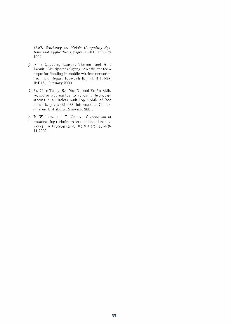
C !$)(*)0* )*6 ) #)-&X 9 : )5 6 1 09&14:5 0 +8, 6-689 ./+1 ) 0V T[ 0 6 2O 66 <¡T°D01010 ¥

¿ Ë ' I>°Q°Q¡$ ¡< <[ $T Ë ¡ @¥²¡ 8 :<>°Q TÖ Ë #` <¹[¨vÏ¡¢~­TQvv `' LB < [~Yv<¥¬¹[¨<L³B<8r$³B[r[¨)³B<8rm³¢³  0 ¦ Ì ³B¦ Ë <¡T° à 666¥

% ;~¡vrÕ¶¨<¬Br<T Í<';¶ Ì @ 8T~v';~¡ ¨ ¨j¥Ë v «w¨[/f< <«Q f<YY&# ªB < [##¡ ¨F' ¨vYO¥TT[ 92 - ¥[¦§<T TOÕ¶v<r<T£ Y ¡v[ °vY<&< à 66 ¥

I¥L¼) &Tw¬£¥©Õ'j¥ Õ¶'Tr <Y B[¨Ï¡[¹:' #¨v¶rv<¥¢¦§ (*)./:/:/,R0)5 ?C # : ¡ 0 ©Ã 66 à ¥

Adaptive Handover Control in IP-based Mobility Networks

Taeyeon Park and Arek DadejCooperative Research Centre for Satellite Systems

Institute for Telecommunications Research, University of South AustraliaMawson Lakes Boulevard, Mawson Lakes, SA 5095, Australia

Email: typark@spri.levels.unisa.edu.au, arek.dadej@unisa.edu.au

Abstract

In this paper, we propose framework for an AdaptiveHandover Control Architecture (AHCA), which aimsat enhancing overall handover performance while max-imising utilisation of scarce resources in wireless accessnetworks. The handover using the AHCA adapts dy-namically to network conditions, as well as a wide rangeof user profiles and application Quality of Service re-quirements. To confirm our expectation that AHCA willbring performance benefits in heterogeneous mobile IPnetworking environment, we have investigated basicperformance characteristics of different handover mech-anisms. The preliminary simulation results demonstratethat the AHCA will bring significant performance ben-efits against non adaptive ones.

1 Introduction

Mobile IP (Internet Protocol) [12, 13] provides net-work layer transparent mobility support to mobilenodes (MNs) roaming across different IP subnetworks.Among many deployment issues of Mobile IP, the sup-port for micro (local) mobility and seamless handoverhave been in focus of many research activities over anumber of recent years. While many different proposalssuch as in [8] have been published thus far to addressthese issues, it is generally accepted that one solutioncan not fit all situations and requirements, especially inenvironments where various mobility mechanisms andQuality of Service (QoS) models are mixed together [1]in heterogeneous wireless access networks [10, 14].

There are several reasons why a smart, adaptive han-dover control is needed:

With adaptive handover control, various handoverstrategies can be mixed to take advantage of whateach technique/strategy can offer, depending onthe availability of the technique in a given ac-cess network and the network, user and applicationpreferences.

Adaptive handover control would improve result-ing handover performance as the handover pro-cedures selected will best reflect the dynamicallyvarying network operating conditions.

A number of mobility mechanisms have been pro-posed to achieve effective global and local mobilitymanagement. As a consequence, there is a strongneed to harmonise the use of these different mech-anisms across the entire network.

Normally, some coupling between layer-3 andlayer-2 is required (layer-2 support) to achieve besthandover performance with the different accessnetwork technologies.

Heterogeneous wireless access technologies re-quire specific handover strategies suited for eachwireless access network, resulting in a need for acommon framework to make handover across thedifferent access technologies seamless.

To best adapt to the current operating conditions andthe access network environment where a MN has justmoved into, it would be preferable if a smart (adaptive)handover control mechanism [3] could provide flexibleservice depending on dynamically varying requirementsof each traffic flow and application session involved [2].For this purpose, we have designed the Adaptive Han-dover Control Architecture (AHCA). As a core part ofthe architecture, the Adaptive Handover Engine takesinputs from several input pre-processing modules, e.g.network resource information from the Network Re-source Prober, traffic QoS attributes from the TrafficClassifier, user preferences information from the UserInput Handler, and policy information from the PolicyInput Handler. Then, it selects the best combination ofhandover mechanisms using a handover adaptation al-gorithm, so that the chosen handover strategy producesthe best performance for the user, while minimising theuse of shared network resources. The architecture hasbeen inspired by the related research in the field of Mo-bile IP handoff control, such as Programmable Hand-offs [4], Policy-Enabled Handoffs [15], and many otheradaptive or feedback-based control approaches [5, 7, 6].

As an example, the AHCA can be applied to the envi-ronment where interoperation of terrestrial and satellitewireless mobile networks is required [11]. In a sim-ple scenario of a satellite-to-terrestrial handover case,the optimal handover control would force handover assoon as an available terrestrial mobile network can be

found, thus increasing user satisfaction in terms of bothperformance and cost. The details of our example sce-nario would change according to varying conditions sur-rounding MN, thus would require some form of adapta-tion which can be accomplished within the AHCA.

The design goals for the AHCA can be summarisedas follows:

Seamless (both low-loss and low-latency) han-dover, adaptive in respect to specific requirementsof traffic type and its explicit or implicit QoS at-tributes

Microflow based handover control, supportingboth user and terminal mobility

Fairness- or priority-based usage of resources (e.g.bandwidth, buffer memory, power consumptionetc.) while providing reasonable level of QoS

Graceful degradation of QoS in cases of shortagein resource or unavailability of required capability

Dynamic adaptation in pace with varying condi-tions of operating environments and MN itself - au-tomatic or interactive change of operating parame-ters

Backward compatibility with existing standard orde facto standard protocols

Extensibility to cover proposed and future han-dover algorithms and micro-mobility mechanisms

Deployability across a wide range of mobility net-works including 802.11 WLAN (Wireless LocalArea Network) and next generation IP-based cel-lular networks.

The organisation of this paper is as follows: In thenext section, we describe the details of the AHCA. InSec. 3 and 4, we explain the simulation setup andpresent the example network topology used in the sim-ulation study. We then follow with some preliminarysimulation results and their analysis. Finally, we givesome concluding remarks and comments on future di-rections in this research.

2 Adaptive Handover Control Ar-chitecture

Figure 1 shows the basic concept of adaptive handovercontrol (components and flows). The handover adapta-tion algorithm produces optimal set of handover strate-gies according to various inputs. Various inputs - probednetwork information, traffic type and QoS attributes ofa traffic flow, policy control information, and user pref-erence - are fed to the adaptation algorithm to reflect theenvironment within which the handover is to occur. Be-sides these regular inputs, there can be two other pos-sible inputs from the feedback loop and re-adaptation

Traffic

User

ControlPolicy

Prefer.

Type

Handover

AlgorithmAdaptation

Optimal Setof Handover

Strategies

Hashed CacheRe-utilization path

Adaptive Handover Mechanism

Re-adaptation Loop

Probed Network Information

Feedback Loop

HandoverExecution

Figure 1: Concept of Adaptive Handover Control

loop. Feedback loop provides performance measures tothe adaptation algorithm for the purpose of fine-tuningof future handovers. Re-adaptation loop could be usedas a calibration path due to short term changes of sur-rounding network conditions. To speed up the oper-ation, re-utilisation path can be used to save time andresources by utilising a hashed cache table, which is up-dated during a few previous iterations of the control al-gorithm. That could save repetitions of control compu-tations and reduce the time overhead added to the han-dover by the handover control procedures.

In accordance with the basics described in the pre-vious paragraph, we have constructed the AHCA asshown in Figure 2.

The basic operation of the AHCA is as follows. TheAHCA:

a. gathers input information,

b. processes inputs to choose the best set of handovermechanisms, and the best parameters for the mech-anisms selected,

c. controls the execution of the chosen handover byMN and mobility agents (MAs),

d. (optionally) feeds back some performance infor-mation into the handover adaptation engine.

The component processes of the AHCA residemainly in MAs and possibly co-operate with compo-nents of the AHCA residing within the MN. In mostcases, some form of communication needs to occur be-tween MA and MN (or between MAs) to control thehandover execution, and to exchange information thatwill aid handover process. This communication maytake the basic form of handshaking messages and is de-scribed in detail in Sec. 2.1 and 2.4.

The AHCA is designed to be an open architecture sothat the internal details of its component modules canbe substituted as long as the basic interfaces betweenmodules are maintained. In this way, new or more en-hanced mechanisms can be used to increase the per-formance benefits, or mechanisms not available in thegiven access network environment may be substituted

ResourceProber

Network

NetworkResource Info.

Traffic QoSRequirement

TrafficClassifier

Input of UserPreference

User InputHandler

InformationPolicy/Security

Policy InputHandler

Handover

Adaptation

Algorithm

Handover

Enforcer

Evaluation& Feedback

Adaptive Handover Engine Post-ProcessingPre-Processing

Figure 2: Adaptive Handover Control Architecture

with available ones at the expense of some performancedegradation.

Below, we give brief descriptions of the AHCA com-ponent modules, outlining the major inputs and outputsand the main functionality of each module.

Network Resource Prober (NRP): Probe availablenetwork resources, using the Dynamic NetworkResource Probing Protocol, in the neighbouringaccess network and the MN’s home network.

Traffic Classifier (TC): Get QoS attributes via signal-ing protocol related to specific microflow and/orsample data traffic to determine the type of trafficand associated QoS attributes.

User Input Handler (UIH): Process user preferencesinput interactively or via a built-in static interface.

Policy Input Handler (PIH): Query network policy/security/ AAA (Authentication, Authorisation andAccounting) control information and manage localpolicy information (in the form of configuration ta-ble or by dynamic gathering).

Handover Adaptation Algorithm (HAA):Determine the optimal set of handover strate-gies in respect to the obtained input criteria, andfeed them to the handover enforcer.

Handover Enforcer (HEnf): Enforce handover ac-cording to the given set of strategies.

Evaluation and Feedback Processor (EnF): Obtainperformance metrics, evaluate against predefinedthreshold, and feed back to the engine.

In the following subsections, the component modulesof the AHCA are explained in more detail.

2.1 Dynamic Network Resource ProbingProtocol

The Dynamic Network Resource Probing Protocol(DNRPP) can be considered a kind of network re-source discovery protocol used by the Network Re-source Prober module of the AHCA.

The objective of the DNRPP is to probe network re-source information dynamically and in co-operation be-tween MN and MA. Its operation mode can be passiveor active. In passive mode, some information is adver-tised periodically from MA to nearby MNs in an un-solicited manner. In active mode, MN solicits networkresource information from nearby MAs. The MAs re-ceiving the request should repond with requested re-source information unless security association betweenMA and MN has not been established or is broken.

The network resource information will be used as aninput to the HAA as well as to the re-adaptation loop ofthe AHCA. It may also be used in prediction and prepa-ration of future handovers. To effectively aid the varioususes of network resource information, it is important toselect the information items most useful to the AHCAand define efficient format of the information as to notconsume too much network bandwidth in the process ofprobing. A few candidates for the components of thenetwork resource information are delay-distance mea-sure between probe initiating node (e.g. MN, FA - For-eign Agent) and probe responding node (e.g. FA, HA -Home Agent, CN - Correspondent Node), and capabili-ties supported by the MN or the MA(s).

2.2 Traffic Classifier

The Traffic Classifier consists of four component mod-ules; three of them are input processor modules, andremaining one is QoS level classifier module. One ofthe input processor modules, the QoS Signal Handler,examines explicit QoS signaling information from vari-ous QoS signaling protocols (e.g. Resource ReservationProtocol Path/Resv, or Multi Protocol Label SwitchingLabel Distribution Protocol) for the specific microflowconcerned, and feeds QoS attributes specified for themicroflow to the Traffic QoS Level Classifier module.The other two input processors are the Header Exam-iner and the Payload Examiner, which respectively ex-amine some IP header fields and a few starting se-quences of payload traffic to get traffic type informa-tion and associated QoS attributes, and then feed thisinformation to the Traffic QoS Level Classifier module.Finally, according to traffic type and associated QoS re-quirements attributes, the Traffic QoS Level Classifier

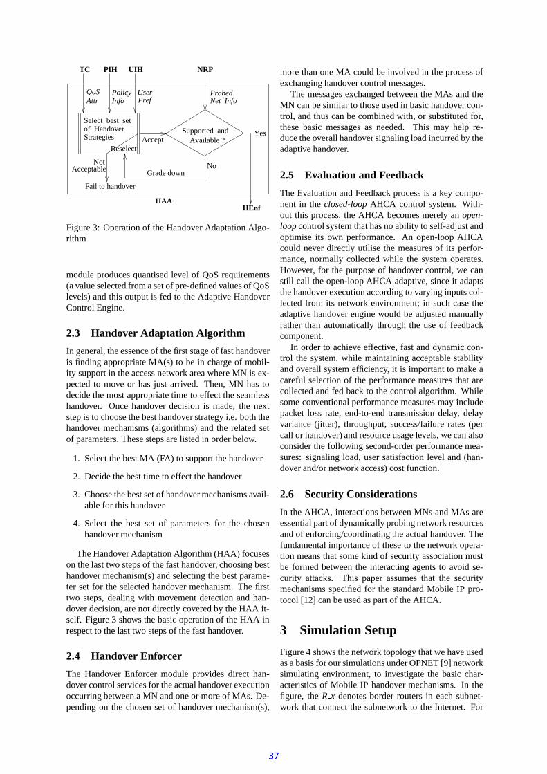
AcceptYes

Reselect

AcceptableNot

Fail to handover

NoGrade down

Probed

Available ?Strategies

QoSAttr Pref

UserPolicyInfo

PIH UIHTC

of HandoverSelect best set

Supported and

HAAHEnf

NRP

Net Info

Figure 3: Operation of the Handover Adaptation Algo-rithm

module produces quantised level of QoS requirements(a value selected from a set of pre-defined values of QoSlevels) and this output is fed to the Adaptive HandoverControl Engine.

2.3 Handover Adaptation Algorithm

In general, the essence of the first stage of fast handoveris finding appropriate MA(s) to be in charge of mobil-ity support in the access network area where MN is ex-pected to move or has just arrived. Then, MN has todecide the most appropriate time to effect the seamlesshandover. Once handover decision is made, the nextstep is to choose the best handover strategy i.e. both thehandover mechanisms (algorithms) and the related setof parameters. These steps are listed in order below.

1. Select the best MA (FA) to support the handover

2. Decide the best time to effect the handover

3. Choose the best set of handover mechanisms avail-able for this handover

4. Select the best set of parameters for the chosenhandover mechanism

The Handover Adaptation Algorithm (HAA) focuseson the last two steps of the fast handover, choosing besthandover mechanism(s) and selecting the best parame-ter set for the selected handover mechanism. The firsttwo steps, dealing with movement detection and han-dover decision, are not directly covered by the HAA it-self. Figure 3 shows the basic operation of the HAA inrespect to the last two steps of the fast handover.

2.4 Handover Enforcer

The Handover Enforcer module provides direct han-dover control services for the actual handover executionoccurring between a MN and one or more of MAs. De-pending on the chosen set of handover mechanism(s),

more than one MA could be involved in the process ofexchanging handover control messages.

The messages exchanged between the MAs and theMN can be similar to those used in basic handover con-trol, and thus can be combined with, or substituted for,these basic messages as needed. This may help re-duce the overall handover signaling load incurred by theadaptive handover.

2.5 Evaluation and Feedback

The Evaluation and Feedback process is a key compo-nent in the closed-loop AHCA control system. With-out this process, the AHCA becomes merely an open-loop control system that has no ability to self-adjust andoptimise its own performance. An open-loop AHCAcould never directly utilise the measures of its perfor-mance, normally collected while the system operates.However, for the purpose of handover control, we canstill call the open-loop AHCA adaptive, since it adaptsthe handover execution according to varying inputs col-lected from its network environment; in such case theadaptive handover engine would be adjusted manuallyrather than automatically through the use of feedbackcomponent.

In order to achieve effective, fast and dynamic con-trol the system, while maintaining acceptable stabilityand overall system efficiency, it is important to make acareful selection of the performance measures that arecollected and fed back to the control algorithm. Whilesome conventional performance measures may includepacket loss rate, end-to-end transmission delay, delayvariance (jitter), throughput, success/failure rates (percall or handover) and resource usage levels, we can alsoconsider the following second-order performance mea-sures: signaling load, user satisfaction level and (han-dover and/or network access) cost function.

2.6 Security Considerations

In the AHCA, interactions between MNs and MAs areessential part of dynamically probing network resourcesand of enforcing/coordinating the actual handover. Thefundamental importance of these to the network opera-tion means that some kind of security association mustbe formed between the interacting agents to avoid se-curity attacks. This paper assumes that the securitymechanisms specified for the standard Mobile IP pro-tocol [12] can be used as part of the AHCA.

3 Simulation Setup

Figure 4 shows the network topology that we have usedas a basis for our simulations under OPNET [9] networksimulating environment, to investigate the basic char-acteristics of Mobile IP handover mechanisms. In thefigure, the R x denotes border routers in each subnet-work that connect the subnetwork to the Internet. For

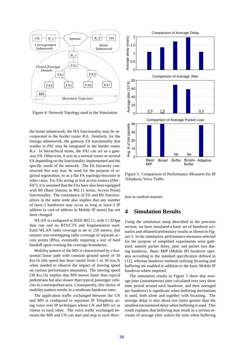
CN

FA4 FA5 FA6 FA7

FA3FA2

FA1

R_v

R_c R_h HAInternet

Visited (Foreign)

CorrespondentSubnetwork

HomeSubnetwork

MNMovement Trajectory

Domain

Figure 4: Network Topology used in the Simulation

the home subnetwork, the HA functionality may be in-corporated in the border router R h. Similarly, for theforeign subnetwork, the gateway FA functionality thatresides in FA1 may be integrated in the border routerR v. In hierarchical terms, the FA1 can act as a gate-way FA. Otherwise, it acts as a normal router or normalFA depending on the functionality implemented and thespecific needs of the network. The FA hierarchy con-structed this way may be used for the purpose of re-gional registration, or as a flat FA topology/structure inother cases. For FAs acting as leaf access routers (FA4 -FA7), it is assumed that the FAs have also been equippedwith BS (Base Station, in 802.11 terms, Access Point)functionality. The coexistence of FA and BS function-alities in the same node also implies that any numberof layer-2 handovers may occur as long as layer-3 IPaddress (a care-of address in Mobile IP sense) has notbeen changed.

WLAN is configured as IEEE 802.11, with 11

data rate and no RTS/CTS and fragmentation used.Each WLAN radio coverage is set to 250 metres; thatensures non-overlapping radio coverage of separate ac-cess points (BSs), eventually requiring a sort of hardhandoff upon crossing the coverage boundaries.

Mobility pattern of the MN is characterised by a hor-izontal linear path with constant ground speed of 30

(the speed has been varied from 1 to 30

when needed to observe the impact of moving speedon various performance measures). The moving speed(30

) implies that MN moves faster than typical

pedestrians but also slower than typical passenger vehi-cles in a metropolitan area. Consequently, this choice ofmobility pattern results in a moderate handover rates.

The application traffic exchanged between the CNand MN is configured to represent IP Telephony us-ing voice over IP techniques where CN and MN act asclients to each other. The voice traffic exchanged be-tween the MN and CN can start and stop in each direc-

0

0.5

1

1.5

2Comparison of Average Delay

Ave

rage

del

ay (

mse

c)

0

20

40

60

80Comparison of Average Jitter

Ave

rage

jitte

r (1

0− 6)

0

10

20

30

40Comparison of Average Packet Loss

Avg

. # o

f los

t pac

kets

Nil Nil

0.3 1.0 0.3

BasicMIP

Bicast Buffer Bicast+Buffer

Adaptive

Figure 5: Comparison of Performance Measures for IPTelephony Voice Traffic

tion in random manner.

4 Simulation Results

Using the simulation setup described in the previoussection, we have simulated a basic set of handover sce-narios and obtained preliminary results as shown in Fig-ure 5. In the simulation, performance measures selectedfor the purpose of simplified experiments were gath-ered, namely packet delay, jitter and packet loss dur-ing handover. Basic MIP (Mobile IP) handover oper-ates according to the standard specification defined in[12], whereas handover methods utilising bicasting andbuffering are enabled in addition to the basic Mobile IPhandover where required.

The simulation results in Figure 5 show that aver-age jitter (instantaneous jitter calculated over very shorttime period around each handover, and then averagedper handover) is significant when buffering mechanismis used, both alone and together with bicasting. Theaverage delay is also about two times greater than thesmallest encountered delay when buffering is used. Thisresult explains that buffering may result in a serious in-crease of average jitter unless the time when buffering

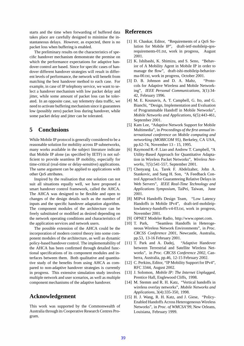
starts and the time when forwarding of buffered datatakes place are carefully designed to minimise the in-stantaneous delays. However, as expected, there is nopacket loss when buffering is enabled.

The preliminary results on the characteristics of spe-cific handover mechanism demonstrate the premise onwhich the performance expectations for adaptive han-dover control are based. Since for specific cases of han-dover different handover strategies will result in differ-ent levels of performance, the network will benefit frommatching the best handover method to each case. Forexample, in case of IP telephony service, we want to se-lect a handover mechanism with low packet delay andjitter, while some amount of packet loss can be toler-ated. In an opposite case, say telemetry data traffic, weneed to activate buffering mechanism since it guaranteeslow (possibly zero) packet loss during handover, whilesome packet delay and jitter can be tolerated.

5 Conclusions

While Mobile IP protocol is generally considered to be areasonable solution for mobility across IP subnetworks,many works available in the subject literature indicatethat Mobile IP alone (as specified by IETF) is not suf-ficient to provide seamless IP mobility, especially fortime-critical (real-time or delay-sensitive) applications.The same argument can be applied to applications withother QoS attributes.

Inspired by the realisation that one solution can notsuit all situations equally well, we have proposed asmart handover control framework, called the AHCA.The AHCA was designed to be flexible and open tochanges of the design details such as the number ofinputs and the specific handover adaptation algorithm.The component modules of the architecture can befreely substituted or modified as desired depending onthe network operating conditions and characteristics ofthe application services and network users.

The possible extension of the AHCA could be theincorporation of modern control theory into some com-ponent modules of the architecture, as well as dynamicpolicy-based handover control. The implementability ofthe AHCA has been confirmed through detailed func-tional specifications of its component modules and in-terfaces between them. Both qualitative and quantita-tive study of the benefits from using AHCA as com-pared to non-adaptive handover strategies is currentlyin progress. This extensive simulation study involvesmultiple network and user scenarios, as well as multiplecomponent mechanisms of the adaptive handover.

Acknowledgement

This work was supported by the Commonwealth ofAustralia through its Cooperative Research Centres Pro-gram.

References

[1] H. Chaskar, Editor, “Requirements of a QoS So-lution for Mobile IP”, draft-ietf-mobileip-qos-requirements-01.txt, work in progress, August2001.

[2] K. Ishibashi, K. Shimizu, and S. Seno, “Behav-ior of A Mobility Agent in Mobile IP in order tomanage the flow”, draft-ishi-mobileip-behavior-ma-00.txt, work in progress, October 2001.

[3] D. B. Johnson and D. A. Maltz, “Proto-cols for Adaptive Wireless and Mobile Network-ing”, IEEE Personal Communications, 3(1):34-42, February 1996.

[4] M. E. Kounavis, A. T. Campbell, G. Ito, and G.Bianchi, “Design, Implementation and Evaluationof Programmable Handoff in Mobile Networks”,Mobile Networks and Applications, 6(5):443-461,September 2001.

[5] Kam Lee, “Adaptive Network Support for MobileMultimedia”, in Proceedings of the first annual in-ternational conference on Mobile computing andnetworking (MOBICOM 95), Berkeley, CA USA,pp.62-74, November 13 - 15, 1995.

[6] Raymond R.-F. Liao and Andrew T. Campbell, “AUtility-Based Approach for Quantitative Adapta-tion in Wireless Packet Networks”, Wireless Net-works, 7(5):541-557, September 2001.

[7] Chenyang Lu, Tarek F. Abdelzaher, John A.Stankovic, and Sang H. Son, “A Feedback Con-trol Approach for Guaranteeing Relative Delays inWeb Servers”, IEEE Real-Time Technology andApplications Symposium, TaiPei, Taiwan, June2001.

[8] MIPv4 Handoffs Design Team, “Low LatencyHandoffs in Mobile IPv4”, draft-ietf-mobileip-lowlatency-handoffs-v4-03.txt, work in progress,November 2001.

[9] OPNET Modeler Radio, http://www.opnet.com.[10] T. Park, “Seamless Handoffs in Heteroge-

neous Wireless Network Environments”, in Proc.CRCSS Conference 2001, Newcastle, Australia,pp.53, 13-16 February 2001.

[11] T. Park and A. Dadej, “Adaptive Handoverbetween Terrestrial and Satellite Wireless Net-works”, in Proc. CRCSS Conference 2002, Can-berra, Australia, pp.46, 12-15 February 2002.

[12] C. Perkins, Editor, “IP Mobility Support for IPv4”,RFC 3344, August 2002.

[13] J. Solomon, Mobile IP: The Internet Unplugged,Prentice Hall, Englewood Cliffs, 1998.

[14] M. Stemm and R. H. Katz, “Vertical handoffs inwireless overlay networks”, Mobile Networks andApplications, 3(4):335-350, 1998.

[15] H. J. Wang, R. H. Katz, and J. Giese, “Policy-Enabled Handoffs Across Heterogeneous WirelessNetworks”, in Proc. of WMCSA’99, New Orleans,Louisiana, February 1999.

On Non-Integer Bits-per-Symbol Modulation in DMT Modems

DANIEL FRANKLIN and IAN BURNETTTelecommunications and IT Research Institute

University of WollongongNorthfields Ave, Wollongong, NSW, 2522

AUSTRALIAd.franklin@ieee.org http://ieee.uow.edu.au/˜daniel

September 16, 2002

Abstract

This paper presents a method for encoding data fortransmission in a discrete multi-tone modem using anon-integral number of bits per symbol. This allowsa more precise assignment of bits per subchannel thanis possible with existing techniques, and is achieved byspreading data over a series of constellations whose sizeis not a power of two. Advantages and disadvantages ofthe proposed technique are discussed.

1 Introduction

Discrete Multi-Tone (DMT) modems are increasinglybeing used in many telecommunications systems, fromADSL modems to the 802.11a and HIPERLAN/2 wire-less standards [1], [2]. They use an efficient form ofOrthogonal Frequency-Division Multiplexing (OFDM),which performs modulation and demodulation by In-verse and Forward Fast Fourier Transforms (FFTs) re-spectively [3], [4]. The block diagram of a conventionalDMT modulator is shown in Figure 1.

Conventional DMT modems use different symbol al-phabets in different subchannels, each with2N

i , N ∈ Zsymbols. The objective of the optimisation algorithmused in most existing DMT modems is to achieve thesame Bit Error Rate (BER) across all subchannels [5].In practice, because of the constraints on the size ofthe constellation, adjustments of the number of bits persymbol in each subchannel can only be performed in avery coarse manner. When a single bit is added or re-moved from a particular subchannel, this causes a dou-bling or halving, respectively, in the size (and, if trans-mission power is constrained, in the density) of the con-stellation. Thus, moving a single bit from one subchan-nel to another in an attempt to even out the BER may

cause a dramatic increase in the BER seen in the recip-ient subchannel. Therefore, it is desirable to be able tomore finely control the dimensions of the constellation.

Techniques exist for encoding data for QAM modemsusing constellations which are not restricted to2N

points. The simplest technique is to use a multidimen-sional generalised cross constellation, as described in[6]. This approach partitions the constellation into anumber of cosets - for example, in the simplest case,consider a constellation with2N + 2N−1 = 3 × 2N−1

points. In any given QAM symbol period, one data bitis used to select the coset, while another group of eitherN or N − 1 bits chooses a point within the coset. Inthis way an average ofN + 0.5 bits is transmitted ineach symbol period. To spread the coset choice evenlyamongst the two cosets, a convolutional code is typi-cally applied to selection bitstream. The concept maybe generalised to choose from amongst2M cosets.

The disadvantage of this technique, however, is thatit does not allow arbitrary constellation size. Accordingto [7], there are modest advantages in hexagonal codes.Further, shell mapping using spherical codes allows formany other constellation sizes in addition to2N [8]. Weattempt to address this disadvantage with a novel tech-nique based on non-binary representations of informa-tion.

2 Non-Integer Bits/Symbol Modu-lation

The Non-Integer Bits/Symbol (NIBS) scheme outlinedhere is based on the extension of the conventional DMTmodulation algorithm. Standard DMT modulation takesa group ofN bits (say, 1024) and breaks it into smallergroups ofMi bits (say, 2-16 bits at a time). Each groupof bits is then used to choose a symbol from an alpha-

1

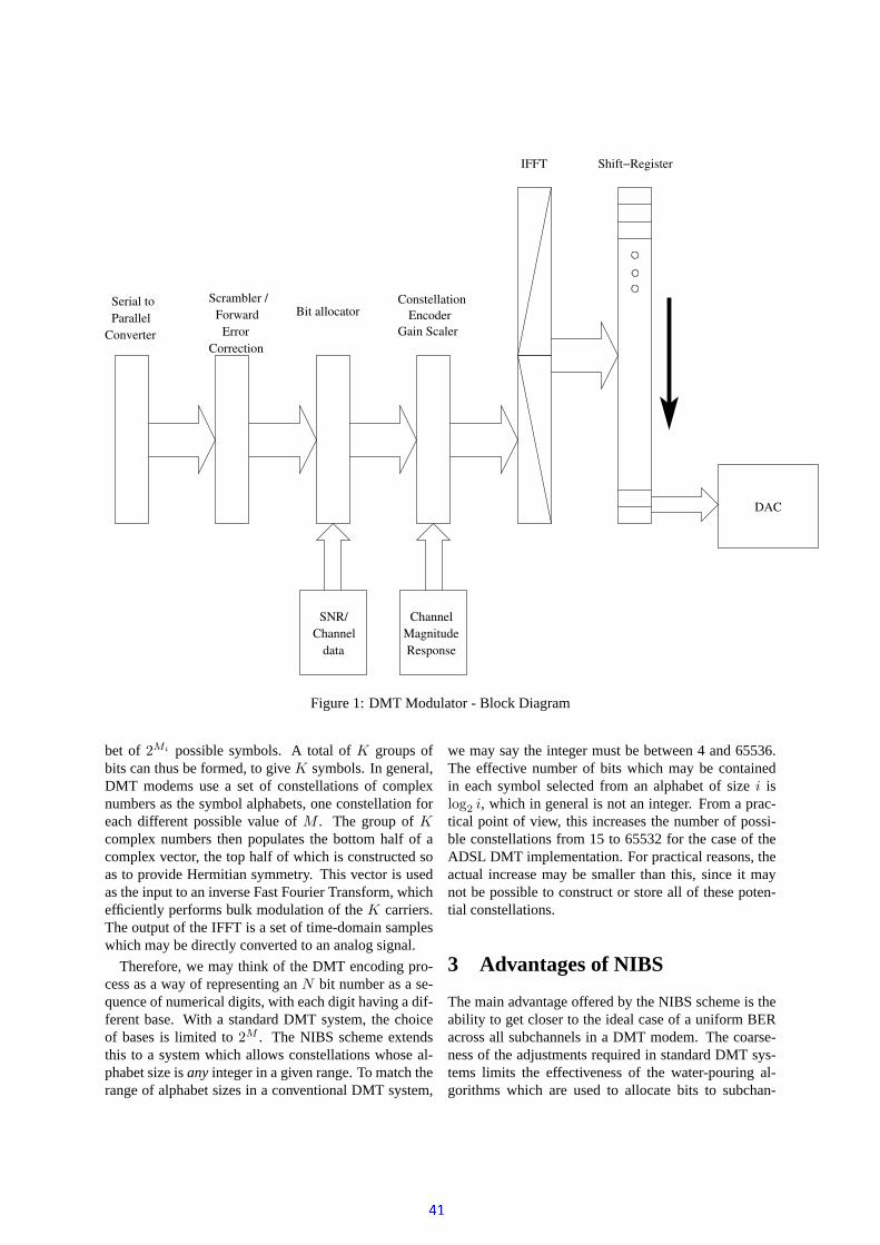
ConstellationEncoder

Shift−Register

Bit allocator

Correction

DAC

Scrambler /

Converter

Magnitude

IFFT

Gain ScalerErrorForward

Serial toParallel

SNR/Channel

data

Channel

Response

Figure 1: DMT Modulator - Block Diagram

bet of 2Mi possible symbols. A total ofK groups ofbits can thus be formed, to giveK symbols. In general,DMT modems use a set of constellations of complexnumbers as the symbol alphabets, one constellation foreach different possible value ofM . The group ofKcomplex numbers then populates the bottom half of acomplex vector, the top half of which is constructed soas to provide Hermitian symmetry. This vector is usedas the input to an inverse Fast Fourier Transform, whichefficiently performs bulk modulation of theK carriers.The output of the IFFT is a set of time-domain sampleswhich may be directly converted to an analog signal.

Therefore, we may think of the DMT encoding pro-cess as a way of representing anN bit number as a se-quence of numerical digits, with each digit having a dif-ferent base. With a standard DMT system, the choiceof bases is limited to2M . The NIBS scheme extendsthis to a system which allows constellations whose al-phabet size isanyinteger in a given range. To match therange of alphabet sizes in a conventional DMT system,

we may say the integer must be between 4 and 65536.The effective number of bits which may be containedin each symbol selected from an alphabet of sizei islog2 i, which in general is not an integer. From a prac-tical point of view, this increases the number of possi-ble constellations from 15 to 65532 for the case of theADSL DMT implementation. For practical reasons, theactual increase may be smaller than this, since it maynot be possible to construct or store all of these poten-tial constellations.

3 Advantages of NIBS

The main advantage offered by the NIBS scheme is theability to get closer to the ideal case of a uniform BERacross all subchannels in a DMT modem. The coarse-ness of the adjustments required in standard DMT sys-tems limits the effectiveness of the water-pouring al-gorithms which are used to allocate bits to subchan-

2

nels. Although NIBS is restricted to a finite numberof constellations, the flexibility it allows is considerablygreater than that available with conventional DMT mod-ulation.

4 Problems and Proposed Solu-tions

The NIBS encoder introduces a number of complica-tions in the encoding process. The first and most im-portant is that is is no longer possible to simply breakup the 1024 bit number into arbitrary groups of of bits.The approach used to encode the number is the samealgorithm as used for changing the digits of a numberfrom one base to another. However, for this to work,it is necessary to have the least-significant digit (LSD)encoded with the largest of our chosen bases (alphabetsizes), and use smaller and smaller bases as we progressto the most-significant digit (MSD). This would at firstseem to destroy the primary benefit to using such DMT,since it limits the choice of allocation of constellationsto subchannels. However, this is not really the case,since the actual order of storing the ‘digits’ (i.e. in theinput vector for the IFFT) is unimportant. Thus, for thepurpose of breaking up the 1024 bit number, the baseused for each digit in the mixed-base representation canbe ranked from largest to smallest (going from LSD toMSD), and the digits can be re-arranged arbitrarily tosuit the SNR per subchannel conditions of the channel.As long as the mapping is known, and can be commu-nicated to the receiver, the transmitted number can bereconstructed in full.

A second problem is that it is not possible to perfectlyrepresent a set of (say) 1024 bits using anything otherthan integer groups of bits without some ‘wasted’ ca-pacity. For example, suppose we wish to transmit a 16-bit number using constellations containing 2, 3, 4, 4,4, 5, 5 and 7 points respectively. The largest numberwhich can be represented in this way would be writtenin mixed-base form as 12333446, or6719910. Thus,our set of digits is sufficient to store 16 bits but not 17bits - and there are a number of possible symbol con-figurations which are not possible (in the range 65536to 67199). However, the system still enjoys the benefitsof being able to more finely tune the dimensions of theconstellation to the SNR conditions of the channel.

The following example illustrates the procedure -suppose we wish to represent the number4729610 us-ing digits with the bases 2, 3, 4, 4, 4, 5, 5 and 7 (call itbaseki):

47300 = 0× (1× 7× 5× 5× 4× 4× 4× 3× 2)++ 1× (1× 7× 5× 5× 4× 4× 4× 3)++ 1× (1× 7× 5× 5× 4× 4× 4)++ 0× (1× 7× 5× 5× 4× 4)++ 3× (1× 7× 5× 5× 4)++ 2× (1× 7× 5× 5)++ 1× (1× 7× 5)++ 1× (1× 7)++ 2× (1)= 11032112ki

The order of these symbols is unimportant, thus forsystems with good SNR at low frequencies and poorSNR at higher frequencies, we may assign the symbolsto subchannels such that the 7-symbol-alphabet digit isgiven the best subchannel, and the 2-symbol-alphabet(i.e. 1-bit) digit is given the worst.

While the two problems described above relate totheoretical aspects of the modulation scheme, the thirdproblem is related to the practicality of implementation.If we are to allow up to 65532 (216 − 4) possible con-stellations, then it is necessary to store these numbers atboth the transmitter end and receiver end. This wouldrequire enough storage to hold approximately231 con-stellation points, or232 single-precision floating-pointnumbers. If a single-precision floating-point number isused to store these values, this will require236 bytesof storage capacity - obviously an impractically largeamount of data. Also, this ignores the difficulties of ac-tually constructing all of these constellations.

Fortunately, many regular constellations can be con-structed algorithmically - therefore, once both transmit-ter and receiver have decided upon the size of eachconstellation, it should be possible for them to designconstellations of this size without the need to store allpossible constellations. These can then be stored in arelatively small lookup table as is done with conven-tional DMT modems. Alternatively, by restricting themaximum size of the constellation to a smaller dimen-sion (for example, 1024 symbols), a smaller capacityis required (the 16-bit constellation is only be rarelyused in practice) which should make storage of the fullset of available constellations possible. Also, it maybe possible to construct a compromise system whichonly includes some constellations which are easy toconstruct algorithmically, such as staggered-concentric-circle APSK, square/pseudo-square as used in conven-tional DMT (see Figure 2(a)), quincunx (see Figure2(b)), hexagonal lattice (see Figures 3(a) and 3(b)) andso on. One particularly interesting aproach, taken from

3

(a) Rectangular (b) Quincunx

Figure 2: 44-point rectangular lattices

(a) Hexagonal, showingfirst four shells (6, 12 and24 points)

(b) Hexagonal +R∠ π

6, showing first

5 shells (3, 9, 12, 18and 24 points)

Figure 3: Hexagonal lattices

the field of vector quantisation (as applied to speechcoding) is described in [9].

The final problem associated with NIBS encodingis the computational complexity of such a system -namely, the large number of multiplications required inthe base conversion process. Fortunately, this task iswell suited to vector processing, and hence implemen-tation on a fixed-point DSP chip should be feasible.

5 Conclusion

DMT modulation based on non-integer bits-per-symbolconstellations should permit a more accurate distribu-tion of data amongst noisy subchnnels. Although thereare a number of problems in the practical realisation ofsuch a scheme, these can be mitigated or eliminated bycareful design of the coder.

References

[1] T1E1.4 Working Group, ANSI T1413-1999 Net-work and Customer Installation Interfaces - Asym-metric Digital Subscriber Line (ADSL) Metallic In-terface, American National Standards Institute,1999.

[2] A. Doufexi, S. Armour, M. Butler, A. Nix, D. Bull,J. McGeehan, and P. Karlsson, “A comparison ofthe HIPERLAN/2 and IEEE 802.11a wireless LANstandards,”IEEE Communications Magazine, vol.40, no. 5, May 2002.

[3] S. B. Weinstein and P. M. Ebert, “Data Transmis-sion by Frequency Division Multiplexing Using theDiscrete Fourier Transform,” IEEE Transactionson Communications Technology, vol. COM-19, pp.628–634, Oct. 1971.

[4] B. Hirosaki, “An Orthogonally Multiplexed QAMSystem Using the Discrete Fourier Transform,”IEEE Transactions on Communications, vol. COM-29, pp. 982–989, July 1991.

[5] John A. Bingham, “Multicarrier Modulation forData Transmission: An Idea Whose Time HasCome,” IEEE Communications Magazine, May1990.

[6] Jr. G. David Forney and Lee-Fang Wei, “Multi-dimensional Constellations - Part I: Introduction,Figures of Merit, and Generalized Cross Constel-lations,” IEEE Journal on Selected Areas in Com-munications, vol. 7, no. 6, Aug. 1989.

[7] G. R. Lang, Jr G. D. Forney, S. Qureshi, F. M.Longstaff, and C. H. Lee, “Signal Structures withData Encoding/Decoding for QCM Modulations,”U.S. Pat. 4 538 284, Aug. 1985.

[8] N. J. A. Sloane, “Tables of Sphere Packings andSpherical Codes,”IEEE Transactions on Informa-tion Theory, vol. 27, pp. 327–338, 1981.

[9] M. A. Ireton and C. S. Xydeas, “On improvingvector excitation coders through the use of spheri-cal lattice codebooks (SLCs),” inICASSP-89, 1989,vol. 1, pp. 57–60.

4

Design of Filterbank Transceivers for Dispersive Channelswith Arbitrary-Length Impulse Response

Alfred Mertins

University of Wollongong

School of Electrical, Computer, and Telecommunications Engineering

Wollongong, NSW 2522, Australia

Abstract

This paper addresses the joint design of transmitter andreceiver for multichannel data transmission over disper-sive channels. The transmitter is assumed to consist ofFIR filters and the channel impulse response is allowedto have arbitrary length. The design criterion is themaximization of the information rate between transmit-ter input and receiver output under the constraint of afixed transmit power. A link to minimum mean squarederror designs for a similar setting is established. Theproposed algorithm allows a straightforward transmit-ter design and generally yields a near-optimum solu-tion for the transmit filters. Under certain conditions,the exact solution for the globally optimal transmitter isobtained.

1 Introduction

The joint design of transmitter and receiver for datatransmission over dispersive channels has attracted nu-merous researchers, as it has the potential to yield veryhigh throughput without the need of costly algorithmson the receiver side, such as maximum likelihood se-quence estimation with the Viterbi algorithm. The pro-cess of shaping the transmit signal and/or introducingredundancy based on the knowledge of the channel isalso known as precoding. Salz [1] provided a first solu-tion to the joint transmit/receive filter design problem,but it required the filters to have support within the firstNyquist zone [1=2T; 1=2T ]. Yang and Roy proposedan algorithm for the design of precoders that use excessbandwidth to introduce redundancy [2]. Their methodrequired an iteration to find the optimum solution. Xiastudied the existence of redundant precoders that allowa perfect inversion of FIR channels with FIR receivers[3]. The effects of noise were not considered in [3]. Di-rect solutions to the joint design problem for the caseof block transforms with a sufficiently long guard inter-val to avoid interblock interference (IBI) were providedin [4–6]. The optimality criteria considered in [4] were

the zero forcing (ZF) and minimum mean squared er-ror (MMSE) criteria. In [5] and [6] the maximizationof mutual information between transmitter and receiverwas studied, using results derived in [7]. A drawbackof the block transforms of [4–6] is that the length ofthe guard interval needs to be at least equal to the chan-nel order. This is the same problem as with the well-known DMT and OFDM techniques [8,9]. To cope withlonger channel impulse responses one can increase thelength of the guard interval, but this will decrease theefficiency, as less data symbols can be transmitted. In-creasing both the length of the guard interval and thenumber of subchannels allows one to maintain a de-sired bandwidth efficiency, but this strategy also has itslimits, because the delay between transmitter and re-ceiver may become unacceptably high. Li and Dingprovided a direct solution to the problem of minimiz-ing the mean squared error (MSE) between transmitterinput and receiver output under the power constraint forarbitrary channel lengths with overlapping blocks [10].However, their solution generally yields IIR transmitfilters, which restricts the practical use of their exact so-lution. An FIR approximation of the technique in [10]was provided in [11]. Finally, transmitter design meth-ods for the case where decision feedback receivers areemployed have been proposed in [7, 12, 13].

This paper addresses the design of FIR precodersfor the case where the channel impulse response hasarbitrary length. Note that this configuration is ofsignificant interest for practical applications, becausereal-world channel impulse responses may become ex-tremely long and the use of sufficiently long guard in-tervals, as required for DMT, OFDM, or the methods in[4–6], may be prohibitive due to delay constraints. Dur-ing transmitter optimization an approximation is usedthat allows us to simplify the objective function and ob-tain a straightforward solution. ForL NM , whereL is the channel order,M is the number of subchannels,and N is the upsampling factor in the transmitter, thealgorithm yields the exact optimum solutions of [5, 6],and forL > NM it leads to near optimum solutions.

h n1( )

h n0( ) NM

M

M

N

Nh nM-1( )

g n0( )

g n1( )

N

N

N

M

M

Mg nM-1( )

x m0 ( )x n( )

x m1 ( )

x mM-1 ( ) y mM-1 ( )

y m1( )

y m0 ( )

c n( )

( )n

z -1z -1

z -1z -1

z -1 y n( )

Figure 1: Redundant precoder.

The paper is organized as follows. Section 2 de-scribes the input-output relationships of the consideredtransmit/receive system. Section 3 then addresses themaximization of the information rate through the choiceof optimal transmit and receive filters. Also a link toMMSE designs for similar settings is established. Sec-tion 4 demonstrates the properties of the proposed algo-rithm in several examples, and finally Section 5 givessome conclusions.

Notation. Vectors and matrices are printed in bold-face. The superscripts fgT , fgH , fg+ denote transpo-sition, Hermitian transposition, and the pseudoinverse.The determinant and trace of a matrix are denoted as j jand tr fg, respectively. E fg is the expectation opera-tion.

2 System Description

A block diagram of the considered system is depictedin Figure 1. The input stream x(m) is split into M par-allel streams which are then upsampled by a factor ofN M and fed into the M transmit filters with im-pulse responses gk(n); k = 0; 1; : : : ;M1. The chan-nel is described by its impulse response c(n) and an ad-ditive, data independent, zero-mean, stationary, Gaus-sian noise process (n). The receive signal is filteredwith the analysis filters hk(n), k = 0; 1; : : : ;M 1and subsampled by N to yield the parallel output datayk(m). Finally, a parallel-to-serial conversion yieldsthe output sequence y(n).

For further analysis it is advantageous to de-compose the filters into their polyphase compo-nents and to describe the system as a multiple-input multiple-output (MIMO) system as depicted inFigure 2. The input vector at time m is givenby x(m) = [x0(m); x1(m); : : : ; xM1(m)]T withxk(m) = x(mMk). Accordingly, the output processy(m) is defined as y(m) = [y0(m); : : : ; yM1(m)]T .The transmit filter bank can be described via its NMpolyphase matrix [14]

G(z) =

264

G00(z) : : : GM1;0(z)...

...G0;N1(z) : : : GM1;N1(z)

375 (1)

where Gk;`(z) is the `th polyphase component of thekth transmit filter, given by

Gk;`(z) =X

ngk(nN + `) zn: (2)

Alternatively, G(z) may be expressed as G(z) =PnGnz

n with [Gn]`;k = gk(nN+`) where [Gn]`;kdenotes the element of [Gn] at position `; k.

The polyphase matrix of the receiver filter bank isgiven by

H(z) =X

nHnz

n

=

264

H 000(z) : : : H 0

0;N1(z)...

...H 0M1;0(z) : : : H 0

M1;N1(z)

375(3)

with

H 0k;`(z) =

Pn hk(nN +N 1 `) zn;

[Hn]k;` = hk(nN +N 1 `):(4)

The channel can be described via the pseudo-circulant N N matrix

C(z) =

26664

C0(z) z1CN1(z) : : : z1C1(z)C1(z) C0(z) : : : z1C2(z)

.... . .

...CN1(z) CN2(z) : : : C0(z)

37775(5)

with C`(z) =P

n c(nN + `) zn. Alternatively,C(z)can be written as a polynomial of matrices:

C(z) =X

kzk Ck: (6)

The often desired (zero forcing) property

y(n) = x(n n0) (7)

is obtained in the noise free case ifH(z) andG(z) arechosen such that the perfect reconstruction (PR) condi-tion

H(z)C(z)G(z) = zn0+1IMM (8)

holds. Conditions to satisfy (7) for a given channel c(n)are for example discussed in [3, 4].

G(

)z

H(

)z

zz

-1C

()

( )n

( )n

N-1( )n

x( )m v( )mN Nx M NxN Mx y( )m

x m0 ( )

y m1 ( )x m1 ( )

y mM-1 ( )x mM-1 ( )

y m0 ( )

Figure 2: Redundant precoder in polyphase (MIMO) representation.

3 Maximizing Information Rate

In this section we address the problem of maximizingthe information rate through the choice of the transmitand receive filters. We will first consider a straightfor-ward matrix model, similar to block transforms, andwill show for this model that the mutual informationcan be expressed via the error covariance matrix ofMMSE receive filters. Using this fact, an algorithm fordetermining optimal FIR transmit filters is presented.

3.1 A General Expression for MutualInformation

The mutual information between a block of input sym-bols, x, and a block of output symbols, y, of atransceiver is defined as I0(x;y) = H(x) H(xjy)where H(x) is the entropy of x and H(xjy) is the con-ditional entropy of x given y [15]. We define a normal-ized mutual information as

I(x;y) =1

N[H(x)H(xjy)] (9)

where N is the upsampling factor in Figure 1. Thelength of x is M with M N , and the length of y willbe defined as needed. It is known that I(x;y) becomesmaximal if x is Gaussian [15], and therefore we willassume Gaussian processes henceforth. For this case itwas shown in [7] that

I(x;y) =1

Nlog2

jRxxjjR?

xjyj

!(10)

withR?xjy = Rxx RxyR

1yyRyx (11)

and Rxx = ExxH

, Rxy = RH

yx = ExyH

,

Ryy = EyyH

.

We now consider the model

y =H[CGx+ n] (12)

where the matrices G;C;H describe the transmitter,channel, and receiver, respectively, and vector n de-scribes additive noise. At this point, no assumptions

are made about the size of vectors and matrices in (12)and the type of noise. With (12) one obtains forR?

xjy

R?xjy = Rxx RxxG

HCHHH[H(CGRxxG

HCH +Rnn)HH ]1

HCGRxx;

(13)

withRnn = EnnH

. By using the pseudoinverse of

R?xjy given by

(R?xjy)

+ = R+xx +

+ GHCHHH [HRnnHH ]1HCG

(14)the quantity I(x;y) can be alternatively expressed as

I(x;y) =1

Nlog2

Rxx (R?xjy)

+: (15)

Note that the expression (14) for (R?xjy)

+ includes theshaping of the transmit signal with matrix G and theinfluence of the receive filters in matrix H. A similarexpression for mutual information has been derived in[7], but for the simpler modely = Cx+nwithn beingwhite noise. Using the results of [7] and a model similarto (12), but without possible interblock interference, arelated expression has also been obtained in [5].

3.2 Incorporating the Filterbank Model

Now let the model (12) describe the filterbanktransceiver of Section 2 with x := x(m) and y :=y(m n0). The columns of matrixG are the transmitfilter impulse responses, and the channel matrix C hasthe structure

C =

26664c(0) 0 0 0 : : : 0c(1) c(0) 0 0 : : : 0c(2) c(1) c(0) 0 : : : 0

......

.... . .

...

37775 : (16)

The size ofC depends on the lengths of the transmit fil-ters and the channel. C may even be of infinite dimen-sion, and similarly, the vector v = CGx+n observedat the channel output may be of infinite length. How-ever, both x and y are of length M . The noise process

n contains the additive channel noise and the IBI fromother data blocks.

In the following we show that the optimal receivematrixH has the structure

H =XGHCHR1nn (17)

with an arbitrary, full-rankM M matrixX. Depend-ing on X one obtains, for example, the ZF or MMSEreceive filters. Inserting (17) into (14) and rearrangingthe obtained expression yields

(R?xjy)

+ = R+xx +GHCHR1

nnCG: (18)

Note that (18) is independent of X. Obviously,(R?

xjy)+ according to (18) is the same as the ma-

trix (R?xjv)

+, which relates to the conditional entropyH(xjv) based on the observation v. Because ofH(xjy) H(xjv), we can conclude that any matrixH of the form (17) maximizes the mutual information.Thus, due to the structure of H in (17) this means thatthe optimal receive filters are “matched filters”, givenby the termGHCHR1

nn , followed by an arbitrary, full-rank matrix operationX. Through the choice ofX onecan obtain, for example, the optimal zero forcing andMMSE solutions.

Interestingly, the matrix (R?xjy) is the same as the

error correlation matrix

R?xjy := Ree = E

(y x)(y x)H

for the case of linear MMSE estimation of x from thenoisy observation v.1 This observation has also beenmade in [7]. For the filterbank transceivers consideredin this papers it means that we can concentrate on min-imizing the determinant of the error correlation matrixin the presence of an MMSE receive filterbank. To sim-plify the notation we assume white channel noise withvariance 2 and white data x(n) with variance 2x. Theincorporation of nonwhite data and noise processes isstraightforward.

For further derivations, the expression (18) for(R?

xjy)+ is not very convenient, as it contains the in-

verse correlation matrix of the noise which is comprisedof channel noise and IBI. Knowing that we need theerror correlation matrix of MMSE estimation we canalternatively use the expression obtained in [11] forMMSE precoders:

Ree =1

2

Z

2x

hIMM+

+2x2GH(ej!)

hXkRcc(k)e

j!kiG(ej!)

i1d!

(19)where

Rcc(k) =X

`CH` C`+k: (20)

1Introductions to linear estimation theory can be found in [16].

3.3 Using FIR transmit filters

To minimize the transmitter complexity and system de-lay, we assume transmit filters of length N where N isthe upsampling factor in Figure 1. For this filter lengthwe haveG(z) =G0 and obtain

Ree =1

2

Z

2x

hIMM

+2x2GH0

hXkRcc(k)e

j!kiG0

i1d!:

(21)The next step is to approximate (21) by a simpler

expression. Because the summation terms for k 6= 0in (21) relate to IBI we choose G0 from a subspacesuch that the terms GH

0 Rcc(k)G0 for k 6= 0 becomeso small that they can be neglected in (21). To deter-mine a suitable subspace for the choice of G0 we em-ploy an iterative procedure based on the singular valuedecomposition (svd). We do not explicitly formulate abasis for the required subspace, and rather consider aprojection P that projects onto the required subspace.

The algorithm is as follows:Step 1: Let P = INN

Step 2: Compute the svd’s

AkkBHk = PH

Rcc(k)P

for all k 6= 0 for whichRcc(k) 6= 0.

Step 3: Determine the largest singular value for k 6= 0and denote it as max. Assuming that max is con-tained in matrixK denote the corresponding col-umn ofAK as a.

Step 4: If rank(P ) > M and max > 0 set

P := [INN aaH ]P

and go back to Step 2. Otherwise, end the algo-rithm.

When incorporating the projection matrix P , the er-ror correlation matrix can be approximated by

~Ree = 2x

hIMM +

2x2GH0 P

HRcc(0)PG0

i1;

(22)and the normalized mutual information can thus be ap-proximated as

I(x;y) =1

Nlog2(jM j) (23)

with

M =hIMM +

2x2GH0 P

HRcc(0)PG0

i: (24)

According to Hadamard’s inequality [15], M must bediagonal in order to maximize jM j under the transmitpower constraint

2x trG0G

H0

= N P0: (25)

This means that the columns of G0 have to be scaledeigenvectors of P H

Rcc(0)P . We now consider theeigendecompositions

PHRcc(0)P = UUH (26)

andG0G

H0 = UQUH (27)

with=diag [1; : : : ; N ] (28)

andQ=diag [q1; : : : ; N ] (29)

where the eigenvalues i are assumed to be sorted suchthat i i + 1. Note that some of the eigenvalues imay be zero and that only the first M values q1; : : : ; qMare non-zero. Using (26) and (27) the mutual informa-tion I(x;y) according to (23) and (24) can be rewrittenas

I(x;y) =1

N

MXi=1

log2(1 +2x2

iqi) (30)

A standard Lagrange optimization, similar to [5, 7],yields

qi = max(c 22xi

; 0) (31)

where c is to be determined from the power constraint(25). As one can see in (31), the optimal values q i obeythe waterpouring distribution. Assuming thatM is cho-sen such that qi, i = 1; : : : ;M are nonzero, the transmitfilters finally become

G0 = U diag [pq1; : : : ;

pqM ] (32)

where U contains theM eigenvectors that belong to thelargest eigenvalues 1; : : : ; M . A comparison with thesolution in [11] shows that maximizing the informationrate and minimizing the overall MSE leads to the sametransmit filters, but with different power loading factorsqi, i = 1; : : : ;M . Moreover, it is straightforward toshow that if the channel order L is smaller or equal toN M we have I(x;y) = I(x;y), and the proposedalgorithm yields the solutions of [5, 6].

4 A Design Example

We demonstrate the performance of the precoder designalgorithm using a simple example where significant IBIbetween adjacent data blocks occurs. The chosen pa-rameters are L = 6, N = 16, M = 14, and the Eb=N0

0 0.05 0.1 0.15 0.2 0.25 0.3 0.35 0.4 0.45 0.5−30

−20

−10

0

10

20

30

normalized frequency

dB

Channel frequency responseTransmit power spectrum (MMSE)Transmit power spectrum (max. Info.)

Figure 3: Channel frequency response and transmitpower spectra.

ratio at the receiver input is set to 20dB. The chan-nel impulse response is c(n) = [1; 1; 1; 1; 1; 1; 1].Note that all channel zeros lie on the unit circle of thez-plane. The frequency response of the channel is de-picted in Figure 3, together with the transmit powerspectra for the following two precoder design meth-ods: (i) the MMSE precoder of [11] and (ii) the pre-coder maximizing information rate proposed in this pa-per. The comparison between the two power spectrashows that the MMSE precoder tends to spend power infrequency bands where the channel gain is low, whereasthe precoder maximizing information rate reduces thetransmit power for such frequencies.

Figure 4 shows the obtained SNR’s at the receiveroutput for the two design methods. One can see thatmaximizing the information rate yields several sub-channels with very good SNR and a few with poorSNR. The MMSE design, on the other hand, tries to up-hold all SNR’s in order to minimize the MSE. The ob-tained normalized information rates are 3.49 bit/symbolfor the MMSE design and 3.84 bit/symbol when maxi-mizing I(x;y).

When reducing the number of subchannels to M =10, all IBI vanishes, and the design method becomesequivalent to the ones in [5,6]. However, the maximumnormalized mutual information is only 3.47 bit/symbolfor this case, which shows that allowing IBI has thepotential to improve performance compared to blocktransmission.

5 Conclusions

A method for the joint design of transmitter and re-ceiver for data transmission over dispersive channelshas been presented. The proposed method maximizesthe information rate and can treat the practically impor-tant case where the transmitter is FIR and the channel

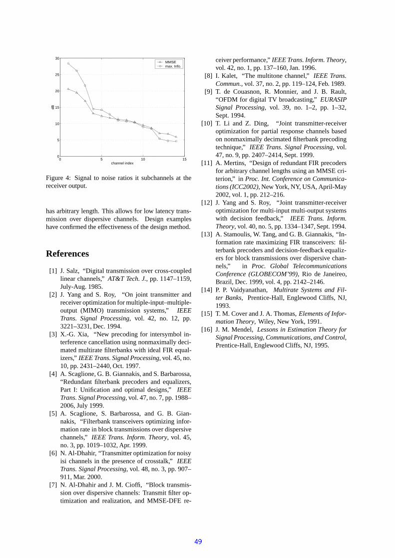
0 5 10 150

5

10

15

20

25

30

dB

channel index

MMSEmax. Info.

Figure 4: Signal to noise ratios it subchannels at thereceiver output.

has arbitrary length. This allows for low latency trans-mission over dispersive channels. Design exampleshave confirmed the effectiveness of the design method.

References

[1] J. Salz, “Digital transmission over cross-coupledlinear channels,” AT&T Tech. J., pp. 1147–1159,July-Aug. 1985.

[2] J. Yang and S. Roy, “On joint transmitter andreceiver optimization for multiple-input–multiple-output (MIMO) transmission systems,” IEEETrans. Signal Processing, vol. 42, no. 12, pp.3221–3231, Dec. 1994.

[3] X.-G. Xia, “New precoding for intersymbol in-terference cancellation using nonmaximally deci-mated multirate filterbanks with ideal FIR equal-izers,” IEEE Trans. Signal Processing, vol. 45, no.10, pp. 2431–2440, Oct. 1997.

[4] A. Scaglione, G. B. Giannakis, and S. Barbarossa,“Redundant filterbank precoders and equalizers,Part I: Unification and optimal designs,” IEEETrans. Signal Processing, vol. 47, no. 7, pp. 1988–2006, July 1999.

[5] A. Scaglione, S. Barbarossa, and G. B. Gian-nakis, “Filterbank transceivers optimizing infor-mation rate in block transmissions over dispersivechannels,” IEEE Trans. Inform. Theory, vol. 45,no. 3, pp. 1019–1032, Apr. 1999.

[6] N. Al-Dhahir, “Transmitter optimization for noisyisi channels in the presence of crosstalk,” IEEETrans. Signal Processing, vol. 48, no. 3, pp. 907–911, Mar. 2000.

[7] N. Al-Dhahir and J. M. Cioffi, “Block transmis-sion over dispersive channels: Transmit filter op-timization and realization, and MMSE-DFE re-

ceiver performance,” IEEE Trans. Inform. Theory,vol. 42, no. 1, pp. 137–160, Jan. 1996.

[8] I. Kalet, “The multitone channel,” IEEE Trans.Commun., vol. 37, no. 2, pp. 119–124, Feb. 1989.

[9] T. de Couasnon, R. Monnier, and J. B. Rault,“OFDM for digital TV broadcasting,” EURASIPSignal Processing, vol. 39, no. 1–2, pp. 1–32,Sept. 1994.

[10] T. Li and Z. Ding, “Joint transmitter-receiveroptimization for partial response channels basedon nonmaximally decimated filterbank precodingtechnique,” IEEE Trans. Signal Processing, vol.47, no. 9, pp. 2407–2414, Sept. 1999.

[11] A. Mertins, “Design of redundant FIR precodersfor arbitrary channel lengths using an MMSE cri-terion,” in Proc. Int. Conference on Communica-tions (ICC2002), New York, NY, USA, April-May2002, vol. 1, pp. 212–216.

[12] J. Yang and S. Roy, “Joint transmitter-receiveroptimization for multi-input multi-output systemswith decision feedback,” IEEE Trans. Inform.Theory, vol. 40, no. 5, pp. 1334–1347, Sept. 1994.

[13] A. Stamoulis, W. Tang, and G. B. Giannakis, “In-formation rate maximizing FIR transceivers: fil-terbank precoders and decision-feedback equaliz-ers for block transmissions over dispersive chan-nels,” in Proc. Global TelecommunicationsConference (GLOBECOM’99), Rio de Janeireo,Brazil, Dec. 1999, vol. 4, pp. 2142–2146.

[14] P. P. Vaidyanathan, Multirate Systems and Fil-ter Banks, Prentice-Hall, Englewood Cliffs, NJ,1993.

[15] T. M. Cover and J. A. Thomas, Elements of Infor-mation Theory, Wiley, New York, 1991.

[16] J. M. Mendel, Lessons in Estimation Theory forSignal Processing, Communications, and Control,Prentice-Hall, Englewood Cliffs, NJ, 1995.

Effects of Phase Noise on Performance of PCC-OFDM

Jinwen Shentu and Jean ArmstrongDepartment of Electronic Engineering, La Trobe University

Victoria 3086, AustraliaEmail: j.shentu@ee.latrobe.edu.au

j.armstrong@ee,latrobe.edu.au

Abstract

This paper investigates the effects of phase noise onthe performance of Polynomial Cancellation CodedOrthogonal Frequency Division Multiplexing (PCC-OFDM). Phase noise will cause two effects on PCC-OFDM, one is a Common Phase Error (CPE) and theother is Interchannel Interference (ICI). CPE isconstant for all subcarriers in a symbol so that it canbe corrected using existing techniques while the ICI isuntracked and contributes to the Bit Error Rate (BER)degradation. It is shown that the ICI cancellationproperties of PCC-OFDM can effectively reduce theICI caused by phase noise.

1. Introduction

In Orthogonal Frequency Division Multiplexing(OFDM) systems, the insertion of the up and downfrequency conversion between the modulator and thedemodulator will almost certainly introduce phasenoise even if zero frequency offset can be achieved[1]. Phase noise is a random perturbation of the phaseof the oscillator’s output signal. It can also beinterpreted as instability of an oscillator. In theliterature [2], phase noise is normally modeled as anideal phase modulation in the oscillator’s signal with aconstant amplitude and unique frequency. The effectsof phase noise on the performance of OFDM systemshave been investigated in the literature [3]. The effectsof the phase noise in an OFDM system result from thecombination of the phase noise in both oscillators ofthe transmitter and the receiver. Without loss ofgenerality, in this paper, the local oscillator in thereceiver will be considered as the phase noise source.

A frequently used model for phase noise in theliterature is where a free-running oscillator isemployed. In this case the phase noise is modeled as aWiener process with zero mean and a Lorentzianpower spectral density [4]. The variance of the phasenoise increases linearly with the time. However, in apractical OFDM system, the frequency of theoscillator is stabilized by means of a phase lockedloop (PLL). The PLL changes the statistics of theoscillator phase noise [5]. Therefore the overall phasenoise spectrum depends on both the properties of thefree-running oscillator and the components of thePLL. In this study we assume that a PLL is always

employed. We will model the phase noise in PCC-OFDM systems as a stationary process with zero meanand a finite variance, the bandwidth of the phase noiseis much smaller than the symbol rate T1 . Thisindicates a slowly varying phase error. In addition, thepower density spectrum is assumed known in thisstudy.

2. Background of PCC-OFDM Polynomial Cancellation Coded OFDM (PCC-OFDM)is a coding scheme for OFDM. PCC-OFDM mapseach data transmitted data onto weighted groups ofsubcarriers [6]. This technique was designed to cancelthe interchannel interference (ICI) caused byfrequency offset [7]. However, in this paper we willshow that PCC-OFDM can also substantially reducethe ICI caused by phase noise.

Figure 1 shows a simplified block diagram of a PCC-OFDM communication system. The high speed QAMdata stream enters a serial to parallel converter to beconverted into n lower speed parallel substreams. Thethi vector to be transmitted is represented by

ini dd ,1,0 ,, − . They are mapped onto the values

iNi aa ,1,0 − that modulate the N subcarriers in the

thi symbol period. For conventional OFDM, Nn =and ikik da ,, = , there is a simple one-to-one mappingof data values onto the subcarriers. In this paper, thecase where each data value to be transmitted ismapped onto pairs of subcarriers is considered, so that

2Nn = .

In the channel, the signal is filtered by the channelresponse ( )th , additive noise ( )tn is injected. At thereceiver the phase noise ( )tθ is introduced. The thioutput vector of the Discrete Fourier Transform (DFT)is iNi zz ,1,0 −

. The demodulated subcarriers are thenweighted and added to generate the data estimates

ini vv ,1,0 − . For a pair of PCC-OFDM subcarriers

iMz ,2 , iMz ,12 + an estimate is calculated using

( ) 2,12,2, iMiMiM zzv +−= .

"!#$%'&)(*+$-,/.0,01243657891:36;<%=?>A@#BC>'D6EGFIHC<<J>LK

3. Phase noise in PCC-OFDM

The thk sample in the thi output vector of theInverse Fast Fourier Transform (IFFT) is given by

∑−

=

=

1

0,,

2exp

1 N

lilik N

klja

Nb

π, 1,,1,0 −= Nk M (1)

where ila , is the thl subcarrier in the thi input vectorof the IFFT. Assuming the additive noise in thechannel is ( )tn with zero mean and finite variance,and the signal is sampled at Nyquist rate, then thereceived signal in the presence of phase noise is givenby

( )( ) ,exp ,,, ikikik nbkjy += θ 1,,1,0 −= Nk M (2)

where ( )kθ is the discrete phase noise of ( )tθ . ikn , is

the thk sample of the additive noise in the thmsymbol. Thus the thm demodulated subcarrier isgiven by

im

N

kikim W

N

kmjyz ,

1

0,,

2exp +

−

= ∑−

=

π(3)

where imW , is the Fast Fourier Transform (FFT) of thechannel noise, which is also Additive White GaussianNoise (AWGN) with zero mean and finite variance.Substituting equation (1) and (2) to (3) gives

( )( )( ) im

N

k

N

lilim Wkj

N

mlkja

Nz ,

1

0

1

0,, exp

2exp

1+

−

= ∑ ∑−

=

−

=θ

π

(4)

Using iMiMiM daa ,,12,2 =−= + for PCC-OFDM, we can

obtain the expression for the th2M PCC-OFDMsubcarrier,

( )

( )( ) ( )( )

iM

N

L

N

k

iLiM

W

kjN

MLkj

NMLkj

dN

z

,2

12/

0

1

0,,2

exp122

exp

4exp

1

+

+−−

−= ∑ ∑

−

=

−

=

θπ

π

(5)

Defining

( )( )∑−

=

−=

1

0exp

2exp

1 N

kn kj

N

knj

Nθ

πψ (6)

where ( ) ( )1,,0,,1 −−−= NNn MM , the thM2subcarrier can be represented by

( )

( ) ( )( ) iM

N

MLL

LMLMiL

iMiM

Wd

dz

,2

12/

0122,

10,,2

+−+

−=

∑−

≠=

−−−

−

ψψ

ψψ(7)

The quantity nψ is the discrete Fourier Transform of( )( )kjθexp , evaluated at the frequency Nn . nψ

depends on the frequency spectrum of the phase noise.The properties of each term in (7) will be analyzedlater after we have derived the expression of therelevant output of the weighting and adding block forthe subcarrier pair. If ( )kθ is a constant, then 0=nψ ,for 0≠n , there is no ICI. Furthermore, for ( ) 0=kθ ,we obtain ,10 =ψ the demodulated subcarrier is equalto its original data to be transmitted.

Under the condition of a small phase noise ( )kθ ,using the approximation ( )( ) ( )kjkj θθ +≈1exp , (7)can be written as

( )( )∑−

=+

−

≈1

01

2exp

1 N

kn kj

N

knj

Nθ

πψ (8)

For 0≠n , (8) is given by

( )∑−

=

−

≈1

0

2exp

N

kn k

N

knj

N

jθ

πψ (9)

nψ is now the FFT of the phase noise, which is thespectrum of the phase noise ( )kθ .

For 0=n , we get

( )∑−

=+≈

1

00 1

N

kk

N

jθψ (10)

)2exp( tfj cπ

P/SDAC

filtering

Highspeeddata

id ,0

ind ,1−

NDivide into low

bit ratestreams

N point IDFT

ib ,0

iNb ,1−

NMappingdata onto

sub-carriers

ia ,0

iNa ,1−

N

Transmitter

Receiver

FilteringADCS/P

NpointDFT

Weight and add

sub-carriers

iy ,0

iNy ,1−

Niz ,0

iNz ,1−

Niv ,0

inv ,1−

NBPF

×

Channel h(t)

n(t)

×

+

exp(j2π(fc+∆f)t+jθ(t))

Similarly we can get the ( )th12 +M demodulatedsubcarrier

( )

( ) ( )( ) iM

N

MLL

LMLMiL

iMiM

Wd

dz

,12

12/

0212,

01,,12

+

−

≠=

−+−

+

+−+

−=

∑ ψψ

ψψ(11)

The corresponding output of the subcarrier pair fromthe weighting and adding block is then given by

( )

( )

( ) ( ) ( )( )∑−

≠=

+−−−−

−

+

−+−+

−+−=

−=

12/

012212,

101,

,12,2,

22

1

22

1

2

N

MLL

LMLMLMiL

iM

iMiMiM

d

d

zzv

ψψψ

ψψψ

(12)

Substituting equation (10) into (12) gives

( )[ ]

( ) ( ) ( )( )

( )

2

221

1221

,12,2

12/

012212,

101,

,,

iMiM

N

MLL

LMLMLMiL

iM

iMiM

WW

d

d

dv

+

−

≠=

−−−+−

−

−+

−+−+

−−+−+

=

∑ ψψψ

ψψψ

(13)

where the first term at the right hand is the wantedsignal, the second term is the Common Phase Error(CPE), the third term is the ICI and the last one is theweighted AWGN noise. In OFDM, the CPE and ICIdepend on the individual frequency spectrum of thephase noise [5]. In PCC-OFDM, the CPE and ICIdepend on the combinations of phase noise spectrarather than individual spectra. This makes it possibleto reduce the effects of phase noise by using a PLLthat can fit the overall phase noise spectrum to aparticular pattern. For the special case where theindividual spectrum nψ has a linear relationship withfrequency, then the ICI caused by the phase noise canbe completely cancelled.

Substituting 1−ψ , 0ψ and 1ψ from (9) and (10) to theCPE term in (13), the CPE term can be obtained by

( )[ ]

( )

( )

0,

1

0

2,

1

0,

101,,

sin2

2cos1

122

1

Θ=

=

−=

−−+−=

∑

∑−

=

−

=

−

iM

N

kiM

N

kiM

iMiCM

jd

kN

kd

N

j

kN

kd

N

j

dY

θπ

θπ

ψψψ

(14)

where 0Θ is a constant, ( )∑−

=

=Θ

1

0

20 sin

2 N

k

kN

k

Nθ

π.

This result indicates that all PCC-OFDM subcarriersexperience a CPE. This rotation can be detected andtherefore compensated using techniques provided inthe literature [8]. One simple way to do this is to insertpilot tones in a symbol and estimate the rotation angle.Once the CPE is corrected in the pilot tones, theremaining phase noise in other subcarriers can becorrected.

Similarly, the ICI term in equation (13) can bepresented by

( ) ( ) ( )( )

( )( )k

N

MLkj

N

kd

N

j

dY

N

MLL

N

kiL

N

MLL

LMLMLMiLiIM

θππ

ψψψ

−

=

−+−=

∑ ∑

∑−

≠=

−

=

−

≠=

−−−+−

4expsin

2

22

1

12/

0

1

0

2,

12/

012212,,

(15)

This term is the contribution of the phase noise to allother subcarriers in a symbol. This result shows thatthe phase noise also causes loss of orthogonality andintroduces ICI. Defining

( )

( )∑−

=−

−

=Θ

1

0

24

expsin2 N

k

ML kN

MLkj

N

k

Nθ

ππ(16)

Equation (15) can be written as

∑−

≠=

−Θ=12

0,,

N

MLL

MLiLiIM djY (17)

We will now investigate the case where phase noise iswhite Gaussian. In this case, no correlation betweenthe samples of phase noise is assumed, the possibledifference between two consecutive samples ishighest. The variance of the CPE can be calculated by

[ ] ( )[ ]

N

kENk

NO N

k

23

sin4

var1

0

24

20

2

θσ

θπ

=

= ∑−

= (18)

where 2θσ is the variance of the phase noise,

( )[ ]22 kE θσ θ = . Note the summation in (18) is a

constant, ( )∑−

==

1

0

4 83sinN

kNNkπ . The variance of the

CPE is proportional to the variance of the phase noise.Thus the variance of the CPE is then given by

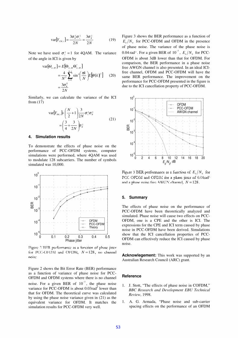
[ ]NN

Y s

iCM 2

3

2

3var

222

,

θθ σσσ== (19)

Note we have used 12 =sσ for 4QAM. The varianceof the angle in ICI is given by

[ ] [ ]

( )[ ]

2

N

kENk

N

EP

N

k

MLMLML

23

sin4

var1

0

24

2

*

θσ

θπ

=

=

ΘΘ=

∑−

=

−−−

(20)

Similarly, we can calculate the variance of the ICIfrom (17)

[ ]

2

3

4

3

2

31

2var

2

22s,

θ

θ

σ

σσ

+=

+=

N

N

NY iIM

(21)

4. Simulation results

To demonstrate the effects of phase noise on theperformance of PCC-OFDM systems, computersimulations were performed, where 4QAM was usedto modulate 128 subcarriers. The number of symbolssimulated was 10,000.

QRSTUVXWYZ\[^]0VLU`_"aUcbdGe0fAVgdAhidX_-Te0fLjkRla7emaC_]0n0d2hVpo R+j-j%VLUq"rsutvvwcxyz|~:6xyz|9

128=N g6'6'0'07-

Figure 2 shows the Bit Error Rate (BER) performanceas a function of variance of phase noise for PCC-OFDM and OFDM systems where there is no channelnoise. For a given BER of

310

−, the phase noise

variance for PCC-OFDM is about 0.03rad2 lower thanthat for OFDM. The theoretical curve was calculatedby using the phase noise variance given in (21) as theequivalent variance for OFDM. It matches thesimulation results for PCC-OFDM very well.

Figure 3 shows the BER performance as a function of0NEb for PCC-OFDM and OFDM in the presence

of phase noise. The variance of the phase noise is0.04 2rad . For a given BER of

310

−, 0NEb for PCC-

OFDM is about 3dB lower than that for OFDM. Forcomparison, the BER performance in a phase noisefree AWGN channel is also presented. In an ideal ICI-free channel, OFDM and PCC-OFDM will have thesame BER performance. The improvement on theperformance for PCC-OFDM presented in the figure isdue to the ICI cancellation property of PCC-OFDM.

C\0L`"c G¡0¢A 2£¤ %¥¡0¢L¦kl7¡9C0NEb

"¥§¨¨©ª«¬­¯®:°6±uª«¬­³²"´¥µp®¶0·0®2¸¹º »+¼-¼-¹Lµp´0²*½¥¾ ½¿#µ?®L± ÀÁGÂ0ÃÁÄÅ0Á2ÆÇ\Â6È7É8ÆÇ*Ê"ËÇAǤÌiÍÏÎXÐÒÑ'Å6Á'ÂÂ0Ç'Ó+Ô 128=N Õ

5. Summary

The effects of phase noise on the performance ofPCC-OFDM have been theoretically analyzed andsimulated. Phase noise will cause two effects on PCC-OFDM, one is a CPE and the other is ICI. Theexpressions for the CPE and ICI term caused by phasenoise in PCC-OFDM have been derived. Simulationsshow that the ICI cancellation properties of PCC-OFDM can effectively reduce the ICI caused by phasenoise.

Acknowlegement: This work was supported by anAustralian Research Council (ARC) grant.

Reference

1. J. Stott, “The effects of phase noise in COFDM,”BBC Research and Development EBU TechnicalReview, 1998.

1. A. G. Armada, “Phase noise and sub-carrierspacing effects on the performance of an OFDM

0 0.1 0.2 0.3 0.4 0.510

-5

10-4

10-3

10-2

10-1

100

Phase jitter

BER

OFDMPCC-OFDMTheory

0 2 4 6 8 10 12 14 16 18 2010-5

10-4

10-3

10-2

10-1

100

Eb/N

0, dB

BER

OFDMPCC-OFDMAWGN channel

communication systems,” IEEE CommunicationsLetters, VOL. 2 NO. 1, January 1998.

2. G. V. Klimovitch, “A nonlinear theory of near-carrier phase noise in free-running oscillators,”Proceedings of the 2000 Third IEEE InternationalCaracas Conference on Devices, Circuits andSystems, 2000, pp. T80/1-6, USA.

4. T. Pollet and M. Moeneclaey, “BER sensitivity ofOFDM systems to carrier frequency offset andWiener phase noise,” IEEE Transactions onCommunications, VOL. 43, Feb./Mar./Apr., 1995,pp.191-193.

2. A. Mehrotra, “Noise analysis of phase-lockedloops,” IEEE/ACM International Conference onComputer Aided Design (ICCAD'2000), pp.277-82, 2000, USA.

3. J. Armstrong, "Analysis of new and existingmethods of reducing intercarrier interference dueto carrier frequency offset in OFDM", IEEETransactions on Communication, March 1999,VOL 47, No.3, pp365-369.

4. J. Armstrong, P. M. Grant, and G. Povey,"Polynomial Cancellation Coding of OFDM toreduce Intercarrier interference due to Dopplerspread", IEEE Globecom, 8-12 November, 1998,pp. 2771-2776.

8. J. J. Ye, J. Chen, Y. Qian, Y. L. Tian, “A methodto eliminate effect of phase noise in OFDMsynchronization system,” Journal of ShanghaiUniversity, VOL.3, NO.3, September 1999,pp.214-17.

Capacity of MIMO Wireless Systems, withSpatially Correlated Receive Elements

Leif Hanlen† and Minyue Fu†

School of Electrical Engineering and Computer ScienceThe University of Newcastle, N.S.W. 2308 Australia

eemf,leif@ee.newcastle.edu.au

Abstract— We present a general channel capacitymodel for a random A.W.G.N. channel in the presenceof spatially correlated interference. We consider thecase where the channel is random, and full rank and thenumber of receive elements is allowed to increase indef-initely within a given volume. We show that capacityof the channel does not increase indefinitely for denselypacked elements. Moreover, the limit is governed by thecorrelation properties of the noise and the channel andas such, a power constraint on the receive elements isunnecessary. We examine two cases: the i.i.d. noisecase and the spatially correlated noise case and showthat bounds exist on the capacity in each case. MonteCarlo simulations are used to verify the results.

I. INTRODUCTION

The work of [1], [2] has lead to the concept ofa high capacity MIMO wireless channel, where ca-pacity increases linearly in proportion to the mini-mum number of transmit and receive elements. Theassumptions required for this remarkable capacitygrowth are that the MIMO channel is independent.

More recently, there has been some work suggest-ing that the linear growth is bounded. The work of[3] and [4] has shown that for specific scattering ge-ometries, the linear growth diminishes as the channelbecomes correlated. This has placed limits on point-to-point MIMO channel capacity when the channel isover a large distance.

Further work [5] has shown that an intuitive limiton the channel capacity growth must exist, even inthe presence of so-called “rich scattering” as depictedin [6]. The intuitive limit is developed from the con-cept that for a (small) fixed volume, the total powerreceived by an antenna array cannot increase beyondsome finite limit. This observation seems to contra-dict normal array signal processing theory where thereceived power for a linear array is allowed to in-crease proportionally with the number of receive el-ements, even for a finite transmit power [7]. Otherauthors [8], [9] have also addressed the problem of“dense” receiver elements, however the results sufferfrom an assumption that as receiver elements become

† A part of this work was carried out while the authors vis-ited Nanyang Technological University in Singapore. The authorswould like to thank Nanyang Technological University for theirsupport to this research.

PSfrag replacements

DtDr

Local Scatterers

Rx TxSR

SNinterferers

Fig. 1. Physical arrangement

close, the noise signals received will remain indepen-dent.

We present an antenna model which includes theeffective receive area of the antenna. Following clas-sic electromagnetic theory we show that the receivedpower is proportional to this effective area [10] Thearea model is piece-wise linear. We also conjecturethat as many receivers are added, interference sourceswill have a spatial arrangement. As such, a compo-nent of noise will be passed through a transfer func-tion dependent on the array.

This paper is organized as follows: Section IIpresents an antenna model based on the effective areaof the receiver. This provides a piecewise linearmodel of total power received. Section III developsthe capacity model of the channel, given the powerlimit and the correlation of the received signal andinterference. Section IV provides Monte-Carlo simu-lation results, and V summarizes our results.

II. SCATTERING MODEL

Consider the physical arrangement described infigure 1. A group of NR receivers, arranged in a lin-ear array receive signals from a group of NT transmit-ters, passed through a set of randomly arranged localscatterers SR.

Additionally, the receivers experience interferencefrom a set of distant white sources e. This model re-flects the case for densely packed receivers, where thecontinuous nature of the electromagnetic field meansthat noise sources will begin to exhibit a spatial cor-relation. The interference signals pass through a setof local scatterers SN , where SN may be differentfrom SR. Both sets of scatterers are assumed to be

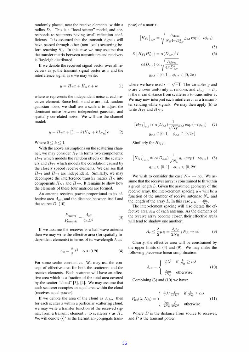
randomly placed, near the receive elements, within aradius Dr. This is a “local scatter” model, and cor-responds to scatterers having small reflection coef-ficients. It is assumed that the transmit signals willhave passed through other (non-local) scattering be-fore reaching SR. In this case we may assume thatthe transfer matrix between transmitters and receiversis Rayleigh distributed.

If we denote the received signal vector over all re-ceivers as y, the transmit signal vector as x and theinterference signal as e we may write:

y = HT x + HNe + w (1)

where w represents the independent noise at each re-ceiver element. Since both e and w are i.i.d. randomgaussian noise, we shall use a scale k to adjust thedominant noise between independent gaussian, andspatially correlated noise. We will use the channelmodel:

y = HT x + [(1 − k)HN + kINR] e (2)

Where 0 ≤ k ≤ 1.With the above assumptions on the scattering chan-

nel, we may consider HT in terms two components:HT1 which models the random effects of the scatter-ers and HT2 which models the correlation caused bythe closely spaced receive elements. We can see thatHT1 and HT2 are independent. Similarly, we maydecompose the interference transfer matrix HN intocomponents HN1 and HN2. It remains to show howthe elements of these four matrices are formed.

An antenna receives power proportional to its ef-fective area Aeff, and the distance between itself andthe source D. [10]

Preceive

Ptransmit=

Aeff

4πD2(3)

If we assume the receiver is a half-wave antennathen we may write the effective area (for spatially in-dependent elements) in terms of its wavelength λ as:

A0 =α

2λ2 α ≈ 0.26 (4)

For some scalar constant α. We may use the con-cept of effective area for both the scatterers and thereceive elements. Each scatterer will have an effec-tive area which is a fraction of the total area coveredby the scatter “cloud” [3], [4]. We may assume thateach scatterer occupies an equal area within the cloud(receives equal power).

If we denote the area of the cloud as Acloud thenfor each scatter s within a particular scattering cloud,we may write a transfer function of the received sig-nal, from a transmit element τ to scatterer s as Hs.We will denote (·)∗ as the Hermitian (conjugate trans-

pose) of a matrix.

[HS1

]s,τ

=

√Acloud

NS4πD2s,τ

gs,t exp (−ιφs,t)

(5)

E HS1H∗

S1 = α(Ds,τ )2I (6)

α(Ds,τ ) ∝√

Acloud

4πD2s,τ

gs,t ∈ [0, 1] , φs,τ ∈ [0, 2π)

where we have used ι =√−1. The variables g and

φ are chosen uniformly at random, and Ds,τ ≈ Ds

is the mean distance from scatterer s to transmitter τ .We may now interpret each interferer n as a transmit-ter sending white signals. We may then apply (6) towrite HT1 and HN1:

[HT1

]s,t

≈ α(Ds,t)1√NS

gs,t exp (−ιφs,t) (7)

gs,t ∈ [0, 1] φs,t ∈ [0, 2π]

Similarly for HN1:

[HN1

]s,n

≈ α(Ds,n)1√NS

gs,nexp (−ιφs,n) (8)

gs,n ∈ [0, 1] φs,n ∈ [0, 2π]

We wish to consider the case NR → ∞. We as-sume that the receiver array is constrained to fit withina given length L. Given the assumed geometry of thereceive array, the inter-element spacing µR will be afunction of the number of receive antennae NR andthe length of the array L. In this case µR = µ0

NR.

The inter-element spacing will also dictate the ef-fective area Aeff of each antenna. As the elements ofthe receive array become closer, their effective areaswill tend to shadow one another:

Ar ≤ λ

2µR =

λµ0

2NR

;NR → ∞ (9)

Clearly, the effective area will be constrained bythe upper limits of (4) and (9). We may make thefollowing piecewise linear simplification:

Aeff =

α2λ2 if L

NR≥ αλ

λµ0

2NRotherwise

(10)

Combining (3) and (10) we have:

Prec(λ,NR) =

α2λ2 P

4πD2 if LNR

≥ αλ

λµ0

2NR

P4πD2 otherwise

(11)

Where D is the distance from source to receiver,and P is the transmit power.

Consider the transfer from the each scatter sr in thescattering cloud SR to the each receiver element r.We can see that there are no multi-path componentsin this transfer, as such the signal at r will be givenby the power received, the phase of the signal at thefirst element in the array and a phase shift due to theposition of r in the array. We may therefore writeHT2, as :

[HT2

]r,sr

≈Prec(λ,NR)1

2 exp

(−ιDsr

2π

λ

)

· exp

(−ιµR

2π

λr sin φsr

) (12)

where Dsr is the mean distance from the local scat-terers to the first receiver in the array and φsr is thebroad-side angle from the array to the scatterer sr.The values of φsr are selected from [0, α] uniformlyat random. The value α < 2π denotes the angularspread of the scatterers as seen from the receive ar-ray. If we write

βsr = exp

(−ιµR

2π

λsinφsr

)(13)

we may write (12) as:[HT2

]r,sr

=Prec(λ,NR)1

2

· exp

(−ιDsr

2π

λ

)(βsr

)r(14)

Likewise for HN2 we may write:[HN2

]r,sn

=Prec(λ,NR)1

2

· exp

(−ιDsn

2π

λ

) (βsn

)r(15)

where the definitions in (15) have the same meaningas (14) with scatterer sr in SR replaced by scatterersn in SN .

Explicitly we now have:

y =HT2HT1x

+ [(1 − k)HN2HN1 + kINR] e

(16)

We may note that the definition of (14) suggests a de-composition of HT2 into two sub-components:

HT2 = VT ΛT (17)

where ΛT is a diagonal matrix, giving the signal gainfrom each scatterer sr and VT is a Vandermonde ma-trix accounting for the term (βsr)

r. We can see thatthe correlation of the signal will be entirely deter-mined by the properties of the matrix VT

[VT

]r,sr

= exp

(−ι

2π

λ

L

NR

r sin φsr

)(18)

which is valid for the approximation that 1

NR→ 0.

If we assume that the D2 losses due to distancefrom scatterer sr to receiver element r are approxi-mately constant for all scatterers in the cloud SR wemay write ΛT as:

[ΛT

]sr,sr

= Prec(λ,NR)1

2 exp

(−ιDsr

2π

λ

)(19)

By similar argument:

HN2 = VSΛS (20)

For completeness we write:

[VT

]r,sn

= exp

(−ι

2π

λ

L

NR

r sin φsn

)

[ΛT

]sn,sn

= Prec(λ,NR)1

2 exp

(−ιDsn

2π

λ

)

We may rewrite (2) using (16), (17) and (20):

y =VT ΛT HT1x

+ [(1 − k)VNΛNHN1 + kINR] e

(21)

Equation (21) provides a general formula for thereceived signal at antenna elements, given both spa-tially correlated and independent noise. The correla-tion of the signal and spatial correlation of the noiseis given by the matrices VT and VN respectively.

We may assume that the receiver applies automaticgain to the signal, such that the power received at eachelement in the array remains constant. In this case, wemay normalise the distance losses and set

ΛT = ΛN = I (22)

This allows us to simplify (21) to:

y = VT HT1x + [(1 − k)VNHN1 + kINR] e (23)

III. CAPACITY

We shall consider the case where the channel is un-known at the transmitter. We assume that the transmitsignal has constant power output independent of NT ,such that:

tr (E xx∗) = E x∗x = P (24)

We shall assume that NT ≥ NR so that any capacityloss will be entirely due to receiver elements. For theunknown channel case, a white transmit signal max-imises the capacity. We may write:

Qx = E xx∗ =P

NT

INT(25)

Let Ψ be the correlation matrix of the completetransfer function for the noise signals e. Then wewrite Ψ as:

Ψ = E[

(1 − k)HN + kI][

(1 − k)HN + kI]∗

(26)

From (8) we can see that in the limit of large NR:

HN1H∗

N1→ INR

(27)

We may use this result and the fact that HN1 and VN

are independent to simplify (26)

Ψ =(1 − k)2E VNV ∗

N + k2E INR

+ k(1 − k)E VNHN + H∗

NV ∗

N(28)

We may interpret the third term in (28) as a cross-correlation between the spatial transfer function andthe i.i.d. direct transfer function. We may view (28)as an interpolation between the two extremes of i.i.d.noise k = 1 and correlated noise k = 0.

Using Ψ we may “whiten” the signal y to give:

y = Ψ−1

2 y

= Ψ−1

2 HT x + HNe (29)

where HN is white:

E

HN HN

∗

= INR

If we define C as the capacity of the channel, then

C = EHN ,Ψ

−

1

2 HT

Ex,e [log det (yy∗)]

Since x and e are independent, we may use the stan-dard form of [1]:

C = E

log2 det

(P

NT

HT H∗

T Ψ−1 + INR

)

(30)We shall now consider the two extreme cases k = 0

and k = 1 for the noise sources. For other situationswhere 0 < k < 1 we may evaluate (30) numerically.

A. Independent Identically Distributed Noise: k = 1

From (28) we may see that Ψ = INRand we may

write (30) as:

C = E

log2 det

(P

NT

HT H∗

T + INR

)(31)

which is the standard result from [1]. However, thematrix HT is not i.i.d. However, from (7) and theweak law of large numbers, we can see that:

1

NT

HT H∗

T → EVT |ΛT |2V ∗

T

(32)

as NT becomes large (see appendix). Using the aboveassumptions (22) we may then write:

1

NT

HT H∗

T → E VT V ∗

T (33)

We now wish to evaluate the expression E VT V ∗T .

We may firstly note that by definition, any Vander-monde matrix VT may be written as:

VT =

1v

v ⊗ v...

v⊗NR−1

where v is a row vector of independent elements, ⊗denotes the element-wise product and (·)⊗k denotesrepeated application of ⊗. As the ordering of the scat-terers in (18) is not important, without loss of gener-ality we may assume that the values vi = βsr arearranged in ascending order. Further, as the valuesof φsr are uniformly distributed, we may assume thatas the NR becomes large, the element values will ex-actly match their distribution - and become uniformover the interval [0, 2π)

If we approximate the eigenvectors of the matrixVT by the vectors v⊗k then the eigenvalues ξk VT will be given by:

ξk VT ≤ Ev⊗kv∗⊗k

where the inequality becomes equality when the ap-proximation of the eigenvectors becomes exact.

We may now write a limit for the eigenvalues of thematrix VT V ∗

T :

ξk VT V ∗

T ≤[E

v⊗kv∗⊗k

]2(34)

From [4] we note that as NR becomes large we mayapproximate (34) by:

0 < ξk VT V ∗

T < 2−k (35)

With the above simplifications we may remove theexpectation of (31) and write:

C < 2K log2(NR) +

NR∑

k=1

log2

(1 + P2−k

)

< 2K log2(NR) + P

(1

2

)NR−2

for a constant K. We can see that as NR increases, thebenefit of additional receivers will diminish withoutrequiring an artificial scaling factor. Any shadowingeffects will be in addition to the roll-off in capacitydue to correlation of input signals.

B. Correlated Noise: k = 0

Referring to (28) we have Ψ = E VNV ∗N. For

the case of NS NR we may approximate both HT

and Ψ as follows:

1

NT

HT H∗

T → T [f(α)] (36)

Ψ → T [f(β)]

where T [f(·)] is a Toeplitz matrix. The values α andβ are the respective angular spread of the scattering ofthe transmit signal and the angular spread of the scat-tering of the correlated noise respectively. We maytherefore write the term

HT H∗

T Ψ−1 ≈ T [f(α)]

T [f(β)]= T [f(α) − f(β)] (37)

020

4060

80100

0

0.2

0.4

0.6

0.8

10

5

10

15

20

25

30

35

Number of Receive ElementsScale Factor k

Nor

mal

ised

Cap

acity

Fig. 2. Capacity of channel with increasing numbers of receiversand different values of k

where we have used a well known identity forToeplitz matrices [11]. For α = β we have equal scat-tering angles for both noise and signal and we maywrite:

HT H∗

T Ψ−1 = T [f(α) − f(β)] = T [0] = I

and so (30) simplifies to:

C = NR log2

(1 + K

P

σ2w

)(38)

for a constant K. This provides linear growth in termsof the number of receive elements. For the case wherethe angular spread of the scattering regions is differ-ent, we may bound the eigenvalues of (30) by theeigenvalues of the Toeplitz matrix (37).

However, as NR becomes large, the approximation(36) loses accuracy and so the inverse of Ψ becomeshighly dependent on the distribution of the scatteringplacement - we may note the eigenvalue distributionfrom (34). In this case the capacity growth will di-minish.

This may be interpreted as follows:When we have ‘densely” arranged receive ele-

ments the channel transmitters and receivers becomehighly correlated. If we assume that the MIMO chan-nel H was i.i.d. before we added additional receiveelements, then it is reasonable to expect that for inde-pendent transmitting elements, the channel correla-tion is entirely governed by the spacing of the receiveelements. Likewise, we may consider spatial corre-lation of the noise (interference) as a product of thecorrelation of receive elements.

It is well known [1] that the ideal MIMO chan-nel is one with i.i.d. entries, and due to the convex-ity of the capacity formula (30) any process whichmoves H toward H (an i.i.d. channel) will improvecapacity. Since the interference is correlated by thesame process as the signal, and we expect the originalinterference to be white, whitening the interferenceconsequently de-correlate the incoming signal. Thewhitening matrix Ψ therefore ensures that the entriesof H becomes i.i.d.

0 10 20 30 40 50 60 70 80 90 1000

2

4

6

8

10

12

14

16

18

Number of Receive Elements

Nor

mal

ised

Cap

acity

k = 1: iid noise k = 0: spatially correlated

Fig. 3. Capacity of channel with increasing numbers of receiversfor k = 0 and k = 1

As NR increases, however, small errors in the esti-mation of Ψ begin to have a significant impact on H .Eventually VT and hence Ψ becomes very badly con-ditioned, where the benefits of “whitening” are lost.

IV. SIMULATION

We have tested the channel capacity (30) usingMonte-Carlo simulations of a channel, for increas-ing numbers of receivers. The frequency chosen was3.0GHz, giving λ = 0.1m. We modelled the re-ceivers as being equally spaced along a line L = 5m- becoming progressively closer as the number NR

increased.Scattering was modelled as being placed uniformly

at random over the interval [0, 2π) with different in-stantiations used for the interference and signal paths.

Figure 2 shows the normalised capacity of thechannel plotted as NR is increased for various val-ues of k. Of particular interest are the edges of thesurface, where k = 0 and k = 1. We note that the ca-pacity of the correlated noise channel k ≈ 1 is muchlarger than the capacity of the i.i.d. channel. Thisagrees with intuition, as the noise for the correlatedchannel case may be selectively “cancelled” by Ψ. Sothat the noise power present in the correlated case iseffectively much lower than for the i.i.d. case.

In figure 3 we have plotted the extreme cases ofk = 0 and k = 1 for comparison. The i.i.d. caseis shown with asterisks. The predicted linear growthfor independent elements is shown dashed. We cansee that while the elements remain uncorrelated, thelinear growth of the channel continues proportional tothe number of elements. However, after the elementsbecome correlated, the capacity of the channel beginsto roll-off. This result is consistent with intuition andwith previous results [8].

V. CONCLUSION

We have presented a model for the MIMO channelwhich accommodates spatially correlated noise. Wehave shown that the capacity of the channel will roll-off as the receive elements become densely spaced,

even if the transmitters are independent. This reduc-tion is independent of the power model used for thereceive elements. As such, it is not necessary to con-sider “shadowing” of receive antenna elements to findan upper limit to capacity.

We have also shown that if the dominant noise isspatially arranged - as is the case with interference,then the capacity of the channel is significantly im-prove through the use of the whitening matrix Ψ.However, eventually the correlation effects of thechannel overcome the additional knowledge providedby spatially correlated noise.

APPENDIX

Here we prove the identity for E V DV ∗ whereV is a Vandermonde matrix of a random vector v, andD is a diagonal matrix of a random vector d. V hasNR rows and N columns. We may argue that N ≥NR as for increasing numbers of receivers, we canexpected to detect the presence of increasing numbersof scatterers. Therefore we may write

limNr→∞

N

Nr

= τ ≥ 1

Let v and d have N elements, denoted vk and(1

dk

)2

respectively. V is of the form:

[V

]m,k

= (vk)m

= e−ι 2πmδ

λNRsin φk

φk ∈ [0, α]

[D

]k,k

=

(1

dk

)2

dk ∈ [1, R]

1

N

[V DV ∗

]m,n

=1

N

N∑

k=1

(1

dk

)2

ei(

n−m

NR

)2πδ

λsin φk

(39)

It is clear that the random variables dk and vk areindependent. As such, the random variables Xk =(

1

dk

)2

ei(

m−n

NR

)φk are identically distributed. There-

fore each element Xk in the sum of (39) may be con-sidered to be the result of an independent experiment.From the weak law of large numbers [12], we have:

limN→∞

1

N

N∑

k=1

Xk−→pr

1

N

N∑

k=1

E Xk = E X

limN→∞

1

N

[V DV ∗

]m,n

= E(

1

dk

)2

ei(

n−m

NR

)2πδ

λsin φk

= E(

1

dk

)2E

ei(

n−m

NR

)2πδ

λsin φk

E(

1

x

)2

=1

R

∫ R

1

(1

x

)2

dx

≈ 1

RR 1

E

ei(

n−m

NR

)2πδ

λsin φk

=

1

α

∫ α

0

ei(

n−m

NR

)2πδ

λsin φk dφ

Using an integration of products form we have:

E

ei(

n−m

NR

)2πδ

λsin φk

≈ e

i(

n−m

NR

)2πδ

λsin α

= T [f(α)] (40)

REFERENCES[1] I. E. Telatar, “Capacity of multi-antenna gaussian channels,”

European Transactions on Telecommunications, vol. 10, no.6, pp. 585–595, Nov. 1999.

[2] G. J. Foschini and M. J. Gans, “On limits of wireless com-munications in a fading environment when using multiple an-tennas,” Wireless Personal Communications, vol. 6, pp. 311–335, 1998.

[3] D. Gesbert, H. Bolcskei, D. Gore, and A. Paulraj, “MIMOWireless channels: Capacity and performance prediction,” inIEEE Proc. Globecom00, 2000.

[4] L. Hanlen and M. Fu, “Multiple antenna wireless com-munication systems: Limits to capacity growth,” in IEEEProc. Wireless Communications and Networking Conference,2002, pp. 172–176.

[5] N. Chiurtu, B. Rimoldi, and I. E. Telatar, “Dense multipleantenna systems,” in ITW2001, Cairns, Sept. 2001.

[6] P. W. Wolniansky, G. D. Golden, G. J. Foschini, and R. A.Valenzuela, “V-BLAST: An architecture for realizing veryhigh data rates over the rich-scattering wireless channel,” inProc. ISSSE-98, 1998.

[7] H. Krim and M. Viberg, “Two decades of array signal pro-cessing,” IEEE Signal Processing Magazine, pp. 67–94, July1996.

[8] T. Abhayapala, R. Kennedy, and J. T. Y. Ho, “On capacity ofmulti-antenna wireless channels: Effects of antenna separa-tion and spatial correlation,” in Proc. 3rd AusCTW, 2002, pp.100–104.

[9] J. T. Y. Ho, R. Kennedy, and T. Abhayapala, “Analytic ex-pression for average snr of correlated dual selection diversitysystem,” in Proc. 3rd AusCTW, 2002, pp. 90–94.

[10] M. A. Headl and J. B. Marion, Classic Electromagnetic Radi-ation, Saunders College Publishing, 3rd edition, 1995, ISBN:0-03-097277-9.

[11] B. Ninness, H. Hjalmarsson, and Fredrik Gustafsson, “Gen-eralised fourier and toeplitz results for rational orthonormalbases,” SIAM Journal on Control and Optimization, vol. 37,no. 2, pp. 439–460, 1997.

[12] A. Papoulis, Probability, Random Variables, and StochasticProcesses, McGraw Hill, 1991.

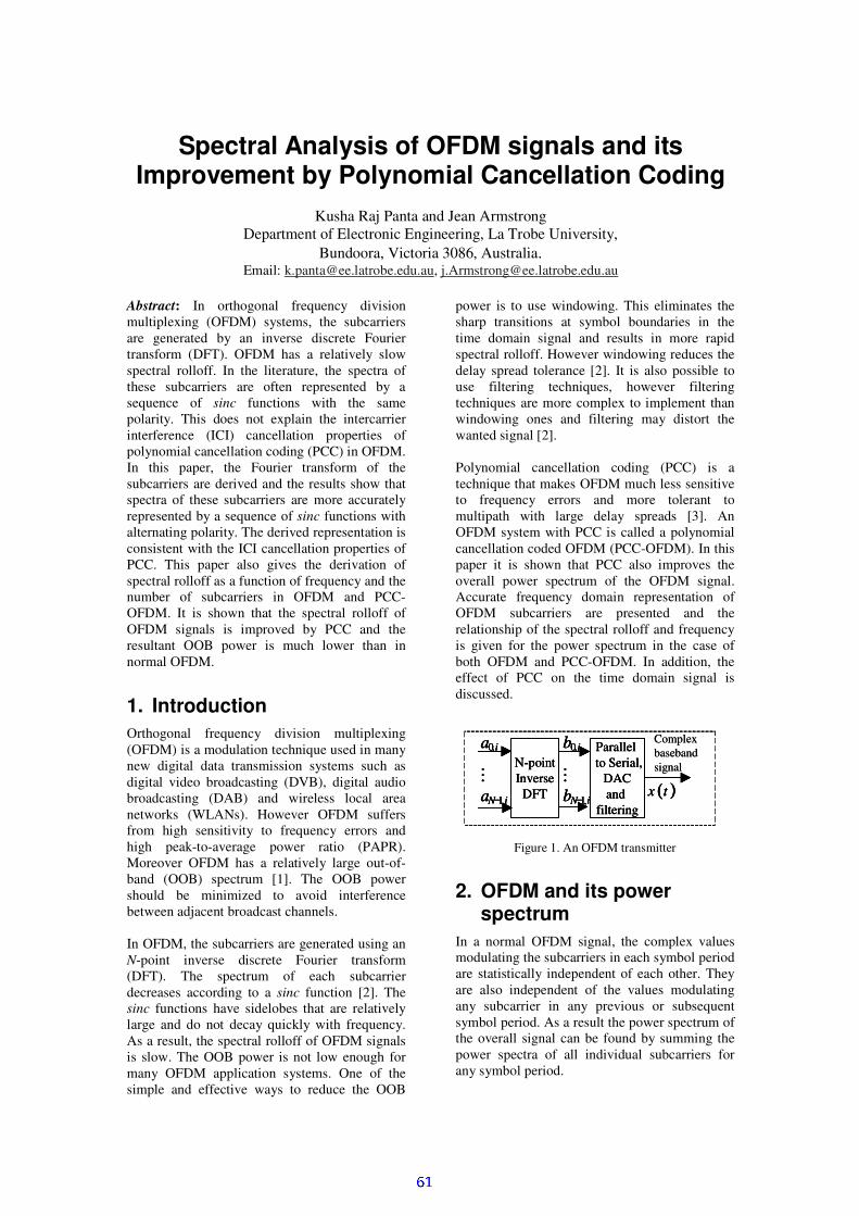
Spectral Analysis of OFDM signals and its Improvement by Polynomial Cancellation Coding

Kusha Raj Panta and Jean Armstrong

Department of Electronic Engineering, La Trobe University, Bundoora, Victoria 3086, Australia.

Email: k.panta@ee.latrobe.edu.au, j.Armstrong@ee.latrobe.edu.au

Abstract: In orthogonal frequency division multiplexing (OFDM) systems, the subcarriers are generated by an inverse discrete Fourier transform (DFT). OFDM has a relatively slow spectral rolloff. In the literature, the spectra of these subcarriers are often represented by a sequence of sinc functions with the same polarity. This does not explain the intercarrier interference (ICI) cancellation properties of polynomial cancellation coding (PCC) in OFDM. In this paper, the Fourier transform of the subcarriers are derived and the results show that spectra of these subcarriers are more accurately represented by a sequence of sinc functions with alternating polarity. The derived representation is consistent with the ICI cancellation properties of PCC. This paper also gives the derivation of spectral rolloff as a function of frequency and the number of subcarriers in OFDM and PCC-OFDM. It is shown that the spectral rolloff of OFDM signals is improved by PCC and the resultant OOB power is much lower than in normal OFDM.

1. Introduction Orthogonal frequency division multiplexing (OFDM) is a modulation technique used in many new digital data transmission systems such as digital video broadcasting (DVB), digital audio broadcasting (DAB) and wireless local area networks (WLANs). However OFDM suffers from high sensitivity to frequency errors and high peak-to-average power ratio (PAPR). Moreover OFDM has a relatively large out-of-band (OOB) spectrum [1]. The OOB power should be minimized to avoid interference between adjacent broadcast channels. In OFDM, the subcarriers are generated using an N-point inverse discrete Fourier transform (DFT). The spectrum of each subcarrier decreases according to a sinc function [2]. The sinc functions have sidelobes that are relatively large and do not decay quickly with frequency. As a result, the spectral rolloff of OFDM signals is slow. The OOB power is not low enough for many OFDM application systems. One of the simple and effective ways to reduce the OOB

power is to use windowing. This eliminates the sharp transitions at symbol boundaries in the time domain signal and results in more rapid spectral rolloff. However windowing reduces the delay spread tolerance [2]. It is also possible to use filtering techniques, however filtering techniques are more complex to implement than windowing ones and filtering may distort the wanted signal [2]. Polynomial cancellation coding (PCC) is a technique that makes OFDM much less sensitive to frequency errors and more tolerant to multipath with large delay spreads [3]. An OFDM system with PCC is called a polynomial cancellation coded OFDM (PCC-OFDM). In this paper it is shown that PCC also improves the overall power spectrum of the OFDM signal. Accurate frequency domain representation of OFDM subcarriers are presented and the relationship of the spectral rolloff and frequency is given for the power spectrum in the case of both OFDM and PCC-OFDM. In addition, the effect of PCC on the time domain signal is discussed.

Figure 1. An OFDM transmitter

2. OFDM and its power spectrum

In a normal OFDM signal, the complex values modulating the subcarriers in each symbol period are statistically independent of each other. They are also independent of the values modulating any subcarrier in any previous or subsequent symbol period. As a result the power spectrum of the overall signal can be found by summing the power spectra of all individual subcarriers for any symbol period.

N-pointInverse

DFT

Parallel to Serial,

DACand

filtering

b

b

i

N i

0

1

,

,

−

a

a

i

N i

0

1

,

,

− ( )x t

Complex baseband signalN-point

InverseDFT

Parallel to Serial,

DACand

filtering

b

b

i

N i

0

1

,

,

−

a

a

i

N i

0

1

,

,

− ( )x t

N-pointInverse

DFT

Parallel to Serial,

DACand

filtering

b

b

i

N i

0

1

,

,

−

b

b

i

N i

0

1

,

,

−

a

a

i

N i

0

1

,

,

−

a

a

i

N i

0

1

,

,

− ( )x t( )x t

Complex baseband signal

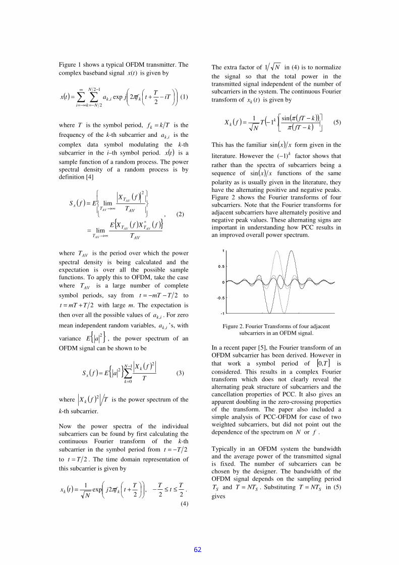
Figure 1 shows a typical OFDM transmitter. The complex baseband signal )(tx is given by

( ) ∞

−∞=

−

−=

−+=i

N

Nkkik iT

Ttfjatx

12

2, 2

2exp π (1)

where T is the symbol period, Tkfk = is the frequency of the k-th subcarrier and ika , is the complex data symbol modulating the k-th subcarrier in the i–th symbol period. ( )tx is a sample function of a random process. The power spectral density of a random process is by definition [4]

( )( )

( ) ( ) AV

TT

T

AV

T

Tx

T

fXfXE

T

fXEfS

AVAV

AV

AV

AV

*

2

lim

lim

∞→

∞→

=

=

, (2)

where AVT is the period over which the power spectral density is being calculated and the expectation is over all the possible sample functions. To apply this to OFDM, take the case where AVT is a large number of complete

symbol periods, say from 2TmTt −−= to

2TmTt += with large m. The expectation is then over all the possible values of ika , . For zero

mean independent random variables, ika , ’s, with

variance 2aE , the power spectrum of an OFDM signal can be shown to be

( ) ( )

−

=

=1

0

22

N

k

kx T

fXaEfS (3)

where ( ) TfX k2 is the power spectrum of the

k-th subcarrier. Now the power spectra of the individual subcarriers can be found by first calculating the continuous Fourier transform of the k-th subcarrier in the symbol period from 2Tt −=

to 2Tt = . The time domain representation of this subcarrier is given by

( )

+=2

2exp1 T

tfjN

tx kk π , 22T

tT ≤≤− .

(4)

The extra factor of N1 in (4) is to normalize the signal so that the total power in the transmitted signal independent of the number of subcarriers in the system. The continuous Fourier transform of )(txk is given by

( ) ( ) ( )( )( )

−−−=kfT

kfTT

NfX k

k ππsin

11

(5)

This has the familiar ( ) xxsin form given in the

literature. However the k)1(− factor shows that rather than the spectra of subcarriers being a sequence of ( ) xxsin functions of the same polarity as is usually given in the literature, they have the alternating positive and negative peaks. Figure 2 shows the Fourier transforms of four subcarriers. Note that the Fourier transforms for adjacent subcarriers have alternately positive and negative peak values. These alternating signs are important in understanding how PCC results in an improved overall power spectrum.

Figure 2. Fourier Transforms of four adjacent

subcarriers in an OFDM signal. In a recent paper [5], the Fourier transform of an OFDM subcarrier has been derived. However in that work a symbol period of [ ]T,0 is considered. This results in a complex Fourier transform which does not clearly reveal the alternating peak structure of subcarriers and the cancellation properties of PCC. It also gives an apparent doubling in the zero-crossing properties of the transform. The paper also included a simple analysis of PCC-OFDM for case of two weighted subcarriers, but did not point out the dependence of the spectrum on N or f . Typically in an OFDM system the bandwidth and the average power of the transmitted signal is fixed. The number of subcarriers can be chosen by the designer. The bandwidth of the OFDM signal depends on the sampling period

ST and SNTT = . Substituting SNTT = in (5) gives

-1

-0 .5

0

0 .5

1

-1

-0 .5

0

0 .5

1

( ) ( )( )( )

−−−=kNfT

kNfTTNfX

S

SkSk π

πsin)1( (6)

And finally, the power spectrum for the subcarrier is given by

( ) ( )( )( )

2sin

−−=kNfT

kNfTTfS

S

SSk π

π (7)

The spectrum of a subcarrier falls of as

( )221 Nf . The overall spectrum being the sum of spectrum of N subcarriers, the OOB spectrum of the complete OFDM signal falls off as ( )Nf 21 . Even for large N , the OOB power is high and a relatively large guard band must be left between different OFDM signals. However a large N results in high PAPR and increased sensitivity to frequency errors [2]. Figure 3 shows the overall power spectra for an OFDM signal for the cases of OFDM systems with 32 and 256 subcarriers. Note the relatively gradual decrease of the OOB power spectrum with frequency.

Figure 3(a). Power spectrum of an OFDM signal with

32 subcarriers

Figure 3(b). Power spectrum for OFDM signal with

256 subcarriers

3. Power Spectrum of PCC-OFDM

In PCC-OFDM, independent data to be transmitted are mapped onto the weighted groups of subcarriers rather than individual subcarriers [3]. For example applying PCC to pairs of adjacent subcarriers gives 10 aa −= , 32 aa −= , and so on. Adjacent pairs must have relative weightings 1+ and 1− . In the general case for groups of m subcarriers the relative weightings are given by the coefficients of the polynomial

1)1( −− mx . The overall power spectrum of the transmitted signal in PCC-OFDM is obtained by first finding the power spectra of all the groups of weighted subcarriers and then by adding the power spectra of these groups. Considering the case of pairs of weighted subcarriers in a group, the Fourier transform the pair of adjacent subcarriers, k -th and )1( +k th, is given by

( ) ( ) ( ) ( )( )( )

( )( ) ( )( )( )

−−−−

+−

−−

=− +

11sin

1cos

sincos1

kNfTkNfT

kTN

kNfTkNfT

kTNfXfX

S

SS

S

SSkk

πππ

πππ

(8) Taking the case of k even and after some manipulation this can be simplified to

( ) ( ) ( )( )( )( )

−−−−−

=− + 1sin

1 kNfTkNfTkNfTTN

fXfXSS

SSkk π

π (9)

And the power spectrum of the weighted subcarrier pair is given by

( )( )( )( )

2

1, 1sin

)(

−−−−=+ kNfTkNfT

kNfTTfS

ss

sskk π

π (10)

The Fourier transform of each weighted pair of subcarriers falls off with an envelope that depends on ( )221 Nf which is faster than the case of OFDM. The overall OOB spectrum of the complete PCC OFDM signal falls off as

( )341 Nf . By similar calculation it can be shown that if weighted groups of three subcarriers are used, the out-of-band spectrum falls off as ( )561 Nf . For the general case of groups of m weighted

0 0.5 1 1.5 2-70

-60

-50

-40

-30

-20

-10

0

10

Frequency

Pow

er S

pect

ral D

ensi

ty (d

B) Number of Subcarriers =

256

0 0.5 1 1.5 2-70

-60

-50

-40

-30

-20

-10

0

10

Number of Subcarriers = 32

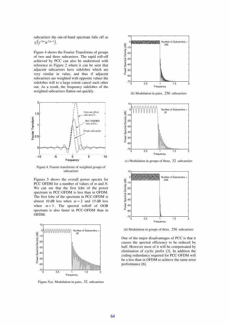
subcarriers the out-of-band spectrum falls off as ( )1221 −mm Nf .

Figure 4 shows the Fourier Transforms of groups of two and three subcarriers. The rapid roll-off achieved by PCC can also be understood with reference to Figure 2 where it can be seen that adjacent subcarriers have sidelobes which are very similar in value, and thus if adjacent subcarriers are weighted with opposite values the sidelobes will to a large extent cancel each other out. As a result, the frequency sidelobes of the weighted subcarriers flatten out quickly.

Figure 4. Fourier transforms of weighted groups of

subcarriers Figures 5 shows the overall power spectra for PCC OFDM for a number of values of m and N. We can see that the first lobe of the power spectrum in PCC-OFDM is less than in OFDM. The first lobe of the spectrum in PCC-OFDM is almost 10 dB less when 2=m and 15 dB less when 3=m . The spectral rolloff of OOB spectrum is also faster in PCC-OFDM than in OFDM.

Figure 5(a). Modulation in pairs, 32 subcarriers

(b) Modulation in pairs, 256 subcarriers

(c) Modulation in groups of three, 32 subcarriers

(d) Modulation in groups of three, 256 subcarriers

One of the major disadvantages of PCC is that it causes the spectral efficiency to be reduced by half. However most of it will be compensated by elimination of cyclic prefix [3]. In addition the coding redundancy required for PCC-OFDM will be a less than in OFDM to achieve the same error performance [6].

0 0.5 1 1.5 2-70

-60

-50

-40

-30

-20

-10

0

10

Frequency

Pow

er S

pect

ral D

ensi

ty (d

B) Number of Subcarriers =

32

0 0.5 1 1.5 2-70

-60

-50

-40

-30

-20

-10

0

10

Frequency

Pow

er S

pect

ral D

ensi

ty (d

B) Number of Subcarriers =

256

0 0.5 1 1.5 2-70

-60

-50

-40

-30

-20

-10

0

10

Frequency

Pow

er S

pect

ral D

ensi

ty (d

B) Number of Subcarriers =

32

0 0.5 1 1.5 2-70

-60

-50

-40

-30

-20

-10

0

10

Frequency

Pow

er S

pect

ral D

ensi

ty (d

B) Number of Subcarriers =

256

4. Windowing effect of PCC in the time domain

In the previous section it is shown that PCC improves the rolloff of OFDM power spectrum and reduces the OOB power. This can also be explained by the considering the effect of PCC in the time domain. For weighted groups of two subcarriers, we have kk aa 212 −=+ . The l-th output component of the transmitter inverse DFT due to the pair of inputs ka2 and 12 +ka is given by

−

=T

ljT

kljab kl

ππ 2exp1

2exp2 (11)

This shows that PCC with data mapped onto weighted subcarrier pairs is equivalent to the windowing of the outputs of the inverse DFT with nonzero inputs on the even numbered subcarriers. The windowing function is complex and is given by ( )( )Tlj π2exp1− . The plot of this window is shown in Figure 6. The plot shows that window is very smooth at the symbol boundaries. The real and imaginary part of this signals are also smooth. This will reduce the OOB power in PCC-OFDM that might otherwise have been caused by the sharp transitions at symbol boundaries. Thus an equivalent system can be built using time domain windowing as shown in Figure 7. In the case of PCC with three weighted subcarriers in a group, it can be easily shown that the windowing function is given by

( )( )Tlπ2cos1 − . This is real and is a Hanning window.

Figure 6. Variation in the power envelope across a symbol period for PCC OFDM. Solid line 2=m , dotted line 3=m .

5. Conclusion The Fourier transform of an OFDM subcarrier is derived and is shown to be of the form

xxk )sin()1(− , where k represents the subcarrier index. Therefore polarity of a particular subcarrier depends on k . The alternating sign on the adjacent subcarriers is consistent with the ICI cancellation properties of PCC in OFDM. The spectral analysis of OFDM is extended to PCC-OFDM. It is shown that PCC improves the spectral rolloff of OFDM signals. The improvement in the spectral rolloff of PCC-OFDM is discussed in the time domain. The effect of PCC in the time domain is windowing. This will result in most of the signal energy being concentrated at the middle of symbol period and smoothing of signals at the symbol boundaries. This will reduce the OOB power in PCC-OFDM.

Figure 7. Time domain equivalent to weighting pairs

of subcarriers Acknowledgement: This study was supported by an Australian Research Council (ARC) grant.

6. References: [1] D. Bhatoolaul and G. Wade, “Spectrum Shaping in N -channel QPSK-OFDM systems”, IEE proc.-Vis. ImageSignal Processing, Vol. 142, 1995, pp. 333-338. [2] R. Van Nee and R. Prasad. OFDM for Wireless Multimedia Communications. Artech House. 2000. [3] J. Armstrong, “Analysis of new and existing method of reducing intercarrier interference due to carrier frequency offset in OFDM,” IEEE Trans. Commun., vol 47, pp. 365-9, March 1999. [4] J. G. Proakis, and M. Salehi. Communication Systems Engineeing. Prentice Hall. 1994. [5] Yuping Z., “In-band and out-band spectrum analysis of OFDM communication systems using ICI cancellation methods,” WCC 2000 - ICCT 2000. 2000 ICCT Proc. IEEE. Part vol.1, 2000, pp.773-6 vol.1. Piscataway, NJ, USA. [6] K. Panta and J. Armstrong, “The performance of Overlap PCC-OFDM with error-correcting codes,” 6th International Symposium on DSP for Communication Systems, Sydney, January 2002, pp.118-122.

-0.5 0 0.50

0.5

1

1.5

2

2.5

3

3.5

4

t/T

Pow

er E

nvel

ope

Complex Window

0

0N-pointInverse

DFT

ioa ,

ia ,2

iNa ,2−

iob ,

iNb ,1−

Complex Window

0

0N-pointInverse

DFT

ioa ,

ia ,2

iNa ,2−

0

0N-pointInverse

DFT

ioa ,

ia ,2

iNa ,2−

iob ,

iNb ,1−

FREQUENCY OFFSET ESTIMATION FOR PCC-OFDM WITHSYMBOLS OVERLAPPED IN TIME DOMAIN

Jinwen Shentu and Jean ArmstrongDepartment of Electronic Engineering, La Trobe University

Victoria 3086, AustraliaEmail: j.shentu@ee.latrobe.edu.au, j.armstrong@ee.latrobe.edu.au

Abstract

This paper presents a new algorithm for frequencyoffset estimation for Polynomial Cancellation CodedOrthogonal Frequency Division Multiplexing withsymbols overlapped in the time domain (OverlapPCC-OFDM). The algorithm exploits the SubcarrierPair Imbalance (SPI) caused by frequency offset. Theestimation is performed in the frequency domain. Notraining symbols or pilot tones are required.Simulations show that this estimator is anapproximately linear function of frequency offset.There are three ways to reduce the variance of theestimation: increasing the number of subcarrier pairs,using a two-dimensional Minimum Mean SquareError (MMSE) equalizer before the estimation andusing PCC-OFDM pilot symbols with no overlapping.

1. Overlap PCC-OFDM Polynomial Cancellation Coded OrthogonalFrequency Division Multiplexing (PCC-OFDM) wasdesigned to reduce the Interchannel Interference (ICI)caused by frequency offset [1]. In PCC-OFDM, eachdata value to be transmitted is mapped onto a group ofsubcarriers. In this paper, the case where each datavalue to be transmitted is mapped onto pairs ofsubcarriers is considered. Despite its advantages,PCC-OFDM is not bandwidth efficient in its simplestform [2]. One way to overcome this drawback is tooverlap PCC-OFDM symbols in the time domain [3].

Figure 1 shows the procedure of symbol overlapping.With overlapping, each overlapped symbol consists ofthree parts, the current PCC-OFDM symbol, thesecond half of the preceding PCC-OFDM symbol andthe first half of the following PCC-OFDM symbol.

Fig. 1 PCC-OFDM symbols overlapped in the timedomain

Figure 2 shows a simplified block diagram of anOverlap PCC-OFDM communication system. The

high speed data stream is fed into a serial to parallelconverter and converted into n lower speed parallelsubstreams. The thi vector to be transmitted isrepresented by ini dd ,1,0 ,, −

. They are mapped onto

the values iNi aa ,1,0 − that modulate the N

subcarriers in the thi symbol period. For conventionalOFDM, which has Nn = and ikik da ,, = , there is a

simple one-to-one mapping of data values onto thesubcarriers. For PCC-OFDM, n and N are not equal.In this paper, we have 2Nn = .

In the channel, the signal is filtered by the channelresponse ( )th and additive noise ( )tn is injected. Atthe receiver the thi output vector of the DFT is

iNi zz ,1,0 − . The demodulated subcarriers are then

weighted and added to generate the data estimatesini vv ,1,0 −

. For the subcarrier pair iMz ,2 and iMz ,12 + ,

an estimate is calculated using( ) 2,12,2, iMiMiM zzv +−= . To recover the transmitted

data values from the overlapped symbols, a two-dimensional Minimum Mean Square Error (MMSE)frequency domain equalizer can be used [3].

Fig. 2. Block diagram of a PCC-OFDM system In [4], a blind frequency offset estimator has beenpresented for PCC-OFDM. As shown in [5], thefrequency offset estimator for PCC-OFDM can alsobe used for PCC-OFDM with symbols overlapped inthe time domain. Recently, a new MMSE frequency

2T

0 2T T 23T T2 Time

ToMMSEEqualizer

Transmitter

Receiver

Divideintolow

bit ratestreams

Parallelto Serial overlap

DAC andfiltering

NpointIDFT

Mappingdata onto

sub-carriers

Highspeeddata

ib ,0

iNb ,1−

ia ,0

iNa ,1−

id ,0

ind ,1−

FilteringADC

Serial toParallel

NpointDFT

iy ,0

iNy ,1−

Weightand add

sub-carriers

iz ,0

iNz ,1−

iv ,0

inv ,1−

h(t)Channel

)2exp( tfj cπ

BPF

))(2exp( tffj c∆+− π

n(t) +

×

×

offset estimator has been proposed for PCC-OFDM[6]. In this paper it will be shown that the same formof the estimator can also be used for Overlap PCC-OFDM.

2. Subcarrier imbalance in PCC-OFDM

In Overlap PCC-OFDM, each demodulated subcarriercontains overlapping components from adjacent PCC-OFDM symbols [4]. The subcarrier pair imbalance isstill defined as the amplitude or power differencebetween two subcarriers in a demodulated subcarrierpair. That is

( ) 2

,2

2

,12 iMiM zzfTF −=∆ + (1)

Each value of imbalance is a combination of theimbalance of the PCC-OFDM subcarrier pair and theimbalance of the overlapping components in thedemodulated subcarrier pair.

In the absence of frequency offset, two demodulatedsubcarriers in an Overlap PCC-OFDM subcarrier pairare balanced in a particular way. The subcarrier pairimbalance depends not only on the frequency offsetand transmitted data values in the current PCC-OFDMsymbol, but also on the overlapping components fromthe preceding and following PCC-OFDM symbols. Asfor PCC-OFDM, the data dependency in OverlapPCC-OFDM can be removed by averaging over anumber of subcarrier pairs. The average subcarrierpair imbalance depends on the frequency offset,therefore, we can use the average imbalance forfrequency offset estimation.

Fig. 3. Subcarrier pair imbalance as a function offrequency offset

Figure 3 shows the average SPI as a function offrequency offset for 32=N . The number ofsimulated subcarriers was 1,000 and all subcarrierpairs were used.

As for PCC-OFDM [6], The figure shows someinteresting features:

• Crossing zero at zero frequency offset.• For 5.0<∆fT , the imbalance increases

monotonically as the frequency offset increases.• Additive White Gaussian Noise (AWGN) does

not affect the zero crossing position.• The frequency estimation range can be extended

to one subcarrier spacing.

3. Expression for an Overlap PCC-OFDMsubcarrier

The thk sample in the thi time domain symbol inPCC-OFDM is given by [2]

∑−

=

=

1

0,,

2exp

1 N

lilik N

klja

Nb

π(2)

where ila , is the thl subcarrier in the thi frequency

domain symbol. The overlapping components in thecurrent symbol are introduced from the second half ofthe ( )th1−i PCC-OFDM symbol and the first half ofthe ( )th1+i PCC-OFDM symbol. The thkoverlapping component is given by [4]

( )

( )

−≤≤

−

−≤≤

−

=

∑

∑

−

=+

−

=−

12for

2exp1

112/0for

2

exp11

1

01,

1

01,

',

Nk N/

N

klja

N

Nk

N

klja

N

bN

lil

l

N

lil

l

ik π

π

(3)

At the receiver, the thk value of the thi input datablock to the FFT demodulator is given by

( ) ikikikik wbbN

kjy ,,

',,

2exp ++

=

επ(4)

where ε is the frequency offset, fT∆=ε . ikw , is the

Gaussian noise. The thm subcarrier in the thidemodulated symbol is then given by

∑∑

∑

−

=

−

=

−

=

−

+

−

=

−

=

1

2,

12

0,

1

0,,

2exp

2exp

2exp

N

Nkik

N

kik

N

kikim

N

kmjy

N

kmjy

N

kmjyz

ππ

π

(5)

The th2M demodulated subcarrier is given by

( ) ( )( )

( ) ( )( )

( ) ( )( )

,2

1

0,122

1

01,122

12

01,122,2

iM

N

LiLMLML

N

LiLMLML

N

LiLMLMLiM

Wdcc

dCSCS

dCFCFz

+−+

++

+=

∑

∑

∑

−

=+−−

−

=++−−

−

=−+−−

(6)

where iMW ,2 is the FFT of ikw , , mlc − are complex

coefficients given by [2]

( )( )NfTmlNj

NfTmlN

fTmlc ml

))(1(exp

)(sin

))(sin(

∆+−−×∆+−∆+−

=−

πππ

(7)

It is shown in [7], iMW ,2 is Gaussian. The coefficients

mlCF − and mlCS − are given by

( )∑

−

=−

+−

=12

0

2exp

1

N

kml N

mlkj

NCF

επ(8)

( )∑

−

=−

+−

=1

2

2exp

1

N

Nkml N

mlkj

NCS

επ(9)

Similarly, the ( )th12 +M demodulated subcarrier canbe obtained.

4. MMSE frequency offset estimator

It is shown in Appendix A that equation (1) forOverlap PCC-OFDM for 4QAM can be written as

( ) ( ) MefTKfTF +∆=∆ πsin (10)

where K is a constant given by [6]

( )

∏−

=

−

=

1log

1

12 2

coscosN

k

k

NNK

ππ(11)

Me is the error term. For small frequency offset, theerror term can be approximated as additive noise withzero mean and finite variance. Applying MMSEtechniques for equation (10) [8], we can obtain thefrequency offset estimator

( )

∆=∆ ∑

=

−lM

tt

l

fTFKM

Tf1

11

sin1ˆπ

(12)

where lM is number of subcarrier pairs to be used forthe frequency offset estimation. 5. Simulation results To evaluate the performance of the MMSE estimator,simulations were performed. In the followingsimulations, 4QAM is used for the modulation schemewith 512=lM and 128=N . Figure 4 shows theestimator as a function of the frequency offset for

dB100 =NEb . It is evident that the estimator has anapproximately linear relationship with frequencyoffset.

Fig. 4. Frequency offset estimator as a function offrequency offset

Fig. 5. Variance of the estimator as a frequency offset

Figure 5 shows the variance of the frequency offsetestimator as a function of the frequency offset for anideal channel. The variance does not changesignificantly as frequency offset increases. This meansthat the overlapping components in Overlap PCC-OFDM are the dominant factor for the variance.Lower variance can be obtained by increasing lM orusing a two-dimensional MMSE equalizer before thefrequency offset estimation. Another way to reducethe variance is to use PCC-OFDM pilot symbols withno overlapping.

Figure 6 shows the variance of frequency offsetestimator as a function of 0NEb . The frequencyoffset simulated was zero. The variance does notsignificantly change as the channel noise increases.The variance is dominated by the overlappingcomponents.∆

fT

-0.5 -0.25 0 0.25 0.5-0.5

-0.25

0

0.25

0.5

Normalized frequency offset

Estim

ator

∆fT

∆fT

^

∆

Fig. 6. Variance of the estimator as a function of0NEb

6. Conclusion

An MMSE frequency offset estimator for OverlapPCC-OFDM has been presented. A frequency offsetestimate is obtained by using the average SPI at theoutput of the receiver FFT. No training symbols orpilot tones are required. The MMSE estimator has anapproximately linear relationship with frequencyoffset. There are three measurements to reduce thevariance, one is to increase the number of subcarrierpairs, the second is to use a two-dimensional MMSEequalizer before the estimation and the third is to usePCC-OFDM pilot symbol with no overlappingcomponents.

Appendix A

From (6), the power of the th2M subcarrier is givenby

( )( )

( )( )

( )( ) iM

N

LiLMLML

N

LiLMLML

N

LiLMLMLiM

edcc

dCSCS

dCFCFz

,2

12/

0

2

,

2

1)(22

12/

0

2

1,

2

1)(22

12/

0

2

1,

2

1)(22

2

,2

+−+

++

+=

∑

∑

∑

−

=+−−

−

=++−−

−

=−+−−

(A.1)

Equation (A.1) indicates that the power of eachdemodulated subcarrier can be represented in terms ofthe individual power components from the preceding,current and following PCC-OFDM symbols. Note for4QAM with each subcarrier normalized to unity,

12

, =iLd . The error term of (A.1) is then given by

( )( ) ( )( )

( )( ) ( )( )

( )( ) ( )( )

( )( ) ( )( )

( )( ) ( )( )

( )( ) ( )( )

( )( ) ( )( )

( )( ) ( )( )

( )( ) Re2

Re2

Re2

2

,2

12/

0

*,

*

1)(22,2

12/

0

*1,

*

)(212,2

12/

0

*1,

*

1)(22,2

,*

1,1)(22

12/

0

12/

0

*

1)(22

1,*,1)(22

12/

0

12/

0

*

1)(22

*,1,

*

1)(22

12/

0

12/

01)(22

*1,,

*

1)(22

12/

0

12/

01)(22

*1,1,

*

1)(22

12/

0

12/

01)(22

*1,1,

*

1)(22

12/

0

12/

01)(22

*,,

*

1)(22

12/

0

12/

01)(22

,2

iM

N

KiKMKMKiM

N

KiKMKMKiM

N

KiKMKMKiM

iKiLMKMK

N

L

N

KMLML

iKiLMKMK

N

L

N

KMLML

iKiLMKMK

N

L

N

KMLML

iKiLMKMK

N

L

N

KMLML

iKiLMKMK

N

KLL

N

KMLML

iKiLMKMK

N

KLL

N

KMLML

iKiLMKMK

N

KLL

N

KMLML

iM

WdccW

dCSCSW

dCFCFW

ddccCFCF

ddCSCScc

ddccCFCF

ddCSCScc

ddCSCSCSCS

ddCFCFCFCF

ddcccc

e

+−+

++

++

+++

+−+

+++

+−+

+++

+++

−−

=

∑

∑

∑

∑ ∑

∑ ∑

∑ ∑

∑ ∑

∑ ∑

∑ ∑

∑ ∑

−

=+−−

−

=+−−−

−

=−+−−

−+−−

−

=

−

=+−−

++−−

−

=

−

=+−−

−+−−

−

=

−

=+−−

++−−

−

=

−

=+−−

+++−−

−

≠=

−

=+−−

−−+−−

−

≠=

−

=+−−

+−−

−

≠=

−

=+−−

(A.2)

Because the expected value of all cross terms is zero,the expected value of the error term is equal to thevariance of the noise. Similarly, we can obtain thepower for the ( )th12 +M subcarrier. Using 1

2

, =iLd

for 4QAM, the subcarrier pair imbalance is then givenby

( )( ) ( )( )

( )( ) ( )( )

( )( ) ( )( )

iMiM

N

LMLML

N

LMLML

N

LMLML

N

LMLML

N

LMLML

N

LMLML

iMiM

ee

cccc

CSCSCFCF

CSCSCFCF

zz

,2,12

12/

0

2

1)(22

12/

0

2

)(212

12/

0

2

1)(22

12/

0

2

1)(22

12/

0

2

)(212

12/

0

2

)(212

2

,2

2

,12

−+

−−−+

+−+−

+++

=−

+

−

=+−−

−

=−−−

−

=+−−

−

=+−−

−

=−−−

−

=−−−

+

∑∑

∑∑

∑∑

(A.3)

It is shown in Appendix B that the combination of thefirst four summations in (A.3) equals zero. Thus wecan obtain the subcarrier pair imbalance

( ) ( ) ',

2

,2

2

,12 iMiMiM efTSzzfTF +∆=−=∆ + (A.4)

where ( )fTS ∆ is given by [6]

( ) ( )fTKfTS ∆=∆ πsin (A.5)

K is a factor defined in (11). ',iMe is the thM total

error, iMiMiM eee ,2,12'

, −= + . In Overlap PCC-OFDM, the

error term is more complicated than in PCC-OFDM.However, the dominant distribution in the error termis still Gaussian. As for PCC-OFDM, '

,iMe can be

Eb/N0, dB

approximated as AWGN with zero mean. Thevariance is larger than that of PCC-OFDM because ofthe overlapping components. Appendix C shows thevariance of the coupling-crossing terms for '

,iMe .

Thus, under the condition of a small frequency offset,the overall approximate variance is given by

( )42', 288 ,0~ nniM Ne σσ ++ (A.6)

where "~" means distributed as. Note that we haveused 12 =sσ for 4QAM in (A.6). The SPI estimator istherefore given by

( )

∆=∆ ∑

=

−lM

ii

l

fTFKM

Tf1

11

sin1ˆπ

(A.7)

Appendix B

The element of the first summation of (A.3) is givenby

( ) ( )( )

( ) ( )

( )( ) ( )

+−

+

−

+−

+

+

=+ −−−

Nsin

12sin

2sin

sin

12

sin

2cos

2

sin

2sin

2

22

2

22

2

2

212

πεπεπ

πε

επ

πε

επ

πε

N

L

N

LN

N

LN

N

LN

CFCF MLML

(B.1)

The element of the second summation of (A.3) isgiven by

( ) ( )( )

( ) ( )

( )( ) ( )

+−

+

+

+−

+

+

=+ −−−

Nsin

12sin

2sin

sin

12

sin

2cos

2

sin

2sin

2

22

2

22

2

2

212

πεπεπ

πε

επ

πε

επ

πε

N

L

N

LN

N

LN

N

LN

CSCS MLML

(B.2)

Similarly the third and fourth terms can be derived.

Substituting the elements derived to the combinationof the first four summations of (A.3) gives

( )( ) ( )( )

( )( ) ( )( )

( ) ( )

0

12sin

2cos

12

sin

2cos

2

22

2

12

022

2

12/

0

2

1)(22

12/

0

2

1)(22

12/

0

2

)(212

12/

0

2

)(212

=

++

−

−+

=

+−+−

+++

∑

∑∑

∑∑

−

=

−

=+−−

−

=+−−

−

=−−−

−

=−−−

N

LN

N

LN

CSCSCFCF

CSCSCFCF

N

L

N

LMLML

N

LMLML

N

LMLML

N

LMLML

επ

πε

επ

πε

(B.3)

Appendix C

The coupling-cross terms iMCC ,2 in (A.2) is given by

( )( ) ( )( )

( )( ) ( )( )

( )( ) ( )( )

( )( ) ( )( ) iKiLMKMK

N

L

N

KMLML

iKiLMKMK

N

L

N

KMLML

iKiLMKMK

N

L

N

KMLML

iKiLMKMK

N

L

N

KMLML

iM

ddccCFCF

ddCSCScc

ddccCFCF

ddCSCScc

CC

,*

1,1)(22

12/

0

12/

0

*

1)(22

1,*

,1)(22

12/

0

12/

0

*

1)(22

*,1,

*

1)(22

12/

0

12/

01)(22

*1,,

*

1)(22

12/

0

12/

01)(22

,2

−+−−

−

=

−

=+−−

++−−

−

=

−

=+−−

−+−−

−

=

−

=+−−

++−−

−

=

−

=+−−

−++

+−+

−++

+−

=

∑ ∑

∑ ∑

∑ ∑

∑ ∑

(C.1)

Similarly, the coupling-cross terms iMCC ,12 + for the

( )th12 +M error term can also be obtained. Note thefirst term and the third term are mutually conjugated,the second term and the fourth term are mutuallyconjugated in (C.1). Thus, iMiM CCCC ,2,12 −+ can be

written as

( ) ( )( ) ( ) ( )( ) ∑

∑−

=−+−−−−

−

=++−−−−

+

++−

++−

=−

12

01,12)(212

*,

12

0

*1,

*

12)(212,

,2,12

2Re2

2Re2

N

LiLMLMLMLiM

N

KiKMKMKMKiM

iMiM

dCFCFCFd

dCSCSCSd

CCCC

(C.2)

where ( )•Re represents the real part of a complexnumber. For the first summation in (C.2), consideringthe most significant complex coefficients 0CS , we get

( ) ( )( )*

1,*0,

12/

0

*1,

*

12)(212,

2

2

+

−

=++−−−−

≈

++∑

iMiM

N

KiKMKMKMKiM

dCSd

dCSCSCSd

(C.3)

Similarly, we can also simplify the second summationin (C.2). In addition, in the absence of frequencyoffset, the value of the most significant complexcoefficient can be obtained from (7) and (8), that is

5.000 == CFCS . Thus (C.2) can be written as

1,*

,*

1,,

,2,12

Re2Re2 −+

+

−−≈−

iMiMiMiM

iMiM

dddd

CCCC(C.4)

The variance of the left side of (C.4) is given by

[ ]( )( ) ( )( )[

( )( ) ( )( )]4

1,*

,*

1,,

2

1,*

,

2*1,,

2

,2,12

8

ReRe4

Re4Re4

s

iMiMiMiM

iMiMiMiM

iMiM

dddd

ddddE

CCCCE

σ=+

+

≈−

−+

−+

+

(C.5)

When all complex coefficients are considered, thevariance will be slightly larger than above result.Please note that this result is obtained under theassumption of no frequency offset. In the presence ofa small frequency offset, the variance could be slightlylarger.

Reference

1. J. Armstrong, "Analysis of New and ExistingMethods of Reducing Intercarrier Interferencedue to Carrier Frequency Offset in OFDM", IEEETransactions on Communications, March 1999,VOL 47, No.3, pp365-369.

2. J. Armstrong, P. M. Grant, and G. Povey,"Polynomial Cancellation Coding of OFDM toreduce Intercarrier Interference due to Dopplerspread", IEEE Globecom, VOL. 5, pp. 2771-2776, 8-12 November, 1998.

3. J. Armstrong, J. Shentu and C. Tellambura,“Frequency Domain Equalization for OFDMSystems with Mapping Data onto Subcarrier Pairsand Overlapping Symbol Periods”. Proceedingsof the 5th International Symposium onCommunication Theory and Applications.England July 1999, pp102-104.

4. J. Shentu and J. Armstrong, "A New FrequencyOffset Estimator for OFDM", "Communicationsystems networks and digital signal processing",edited by A. C. Boucouvalas, pp.13-16, July2000, UK.

5. J. Shentu and J. Armstrong, "Blind FrequencyOffset Estimation for PCC-OFDM with SymbolsOverlapped in the Time Domain". Proceedings ofIEEE ISCAS2001, VOL. 4, pp.570-573, May 6-9,Sydney.

6. J. Shentu, J. Armstrong and G. Tobin, “MMSEFrequency Offset Estimator for PCC-OFDM”,accepted by IEEE MICC’01, 2001.

7. A. Papoulis, "Probability, Random Variables andStochastic Processes," McGraw-Hill InternationalBook Company, 1981.

8. A. Ronald Gallant, "Nonlinear StatisticalModels," John Wiley and sons, 1987.

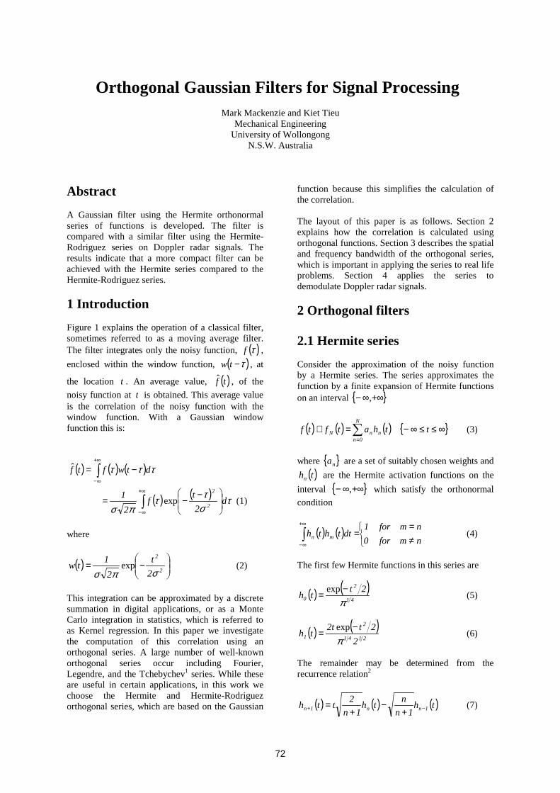
72

Orthogonal Gaussian Filters for Signal Processing

Mark Mackenzie and Kiet Tieu Mechanical Engineering

University of Wollongong N.S.W. Australia

Abstract A Gaussian filter using the Hermite orthonormal series of functions is developed. The filter is compared with a similar filter using the Hermite-Rodriguez series on Doppler radar signals. The results indicate that a more compact filter can be achieved with the Hermite series compared to the Hermite-Rodriguez series. 1 Introduction Figure 1 explains the operation of a classical filter, sometimes referred to as a moving average filter. The filter integrates only the noisy function, ( )τf , enclosed within the window function, ( )τ−tw , at

the location t . An average value, ( )tf , of the noisy function at t is obtained. This average value is the correlation of the noisy function with the window function. With a Gaussian window function this is:

( ) ( ) ( )∫+∞

∞−

−= τττ dtwftf

( ) ( )∫

+∞

∞−

−−= τσττ

πσd

2tf

21

2

2

exp (1)

where

( )

−= 2

2

2t

21tw

σπσexp (2)

This integration can be approximated by a discrete summation in digital applications, or as a Monte Carlo integration in statistics, which is referred to as Kernel regression. In this paper we investigate the computation of this correlation using an orthogonal series. A large number of well-known orthogonal series occur including Fourier, Legendre, and the Tchebychev1 series. While these are useful in certain applications, in this work we choose the Hermite and Hermite-Rodriguez orthogonal series, which are based on the Gaussian

function because this simplifies the calculation of the correlation. The layout of this paper is as follows. Section 2 explains how the correlation is calculated using orthogonal functions. Section 3 describes the spatial and frequency bandwidth of the orthogonal series, which is important in applying the series to real life problems. Section 4 applies the series to demodulate Doppler radar signals. 2 Orthogonal filters 2.1 Hermite series Consider the approximation of the noisy function by a Hermite series. The series approximates the function by a finite expansion of Hermite functions on an interval +∞∞− ,

( ) ( ) ( )thatftf n

N

0nnN ∑

==≅ ∞≤≤∞− t (3)

where na are a set of suitably chosen weights and

( )thn are the Hermite activation functions on the interval +∞∞− , which satisfy the orthonormal condition

( ) ( )

≠=

=∫+∞

∞− nmfor0nmfor1

dtthth mn (4)

The first few Hermite functions in this series are

( ) ( )41

2

02tth

π−

=exp

(5)

( ) ( )2141

2

1 22tt2

thπ

−=

exp (6)

The remainder may be determined from the recurrence relation2

( ) ( ) ( )th1n

nth1n

2tth 1nn1n −+ +−

+= (7)

73

Since the fundamental, ( )th0 , is the Gaussian function it can take the place of the filter function. The correlation integration of equation (1) is then approximately equal to the correlation of the Hermite series with the fundamental Hermite function.

( ) ( ) ( ) ( )∫ ∑+∞

∞− =−

=≅ τττ dthhatftf 0

N

0nnnN

ˆˆ (8)

In order to evaluate this expression, the correlation between the Hermite functions of different order, is required. This correlation is given by 3

( ) ( ) ( )∫+∞

∞−

−=− 2tl21dthh 2mn

mmn τττ ( )nm ≤ (9)

where ( )tl n

m is a normalized associated Laguerre function. Using this result in equation (8) we obtain

( ) ( )∑=

=N

0n

2n0nN 2tla

21tf (10)

Note that only those associated Laguerre functions of subscript 0m = contribute, thus greatly simplifying the result. The associated Laguerre functions of subscript are

( )!n

ettl2t2n

n0

−

= (11)

The usefulness of this expansion is that by fitting a Hermite series to the input function, one also immediately obtains the weights of the Laguerre series, na , which is the correlation of the input with a Gaussian function. 2.2 Hermite Rodriguez Functions Hermite-Rodriguez functions 4,5 are similar to the Hermite functions except that a Gaussian window modulates their amplitude. They are defined as

( ) ( ) ( ) 2tn

41n

2

eththr −= π (12) where ( )thn is an orthonormal Hermite function. The fundamental Hermite-Rodriguez function is also a Gaussian function but of different width to the fundamental Hermite function. The fundamental is

( ) ( )20 exp tthr −= (14)

The others may be determined using the recurrence relation (equation (7)) for the Hermite functions and multiplying by the Gaussian function. Like the Hermite series, a simple expression also occurs for the correlation of the Hermite-Rodriguez functions. The correlation of two Hermite-Rodriguez functions is given by5

( ) ( ) ( ) ( )2thrmn2

mnthrthr mnmnmn ++

+=∗!!

! (15)

Note that the scale is reduced and the order of the Hermite-Rodriguez function increased by the correlation operation. Using equation (15), the derivation of a Gaussian filter with the Hermite-Rodriguez functions is similar to the filter derived using the Hermite series. 3 Method 3.1 Signal duration and bandwidth Application requires the duration and bandwidth of the orthogonal series to be matched to the signal being modeled. The Hermite series behaves as a window in the time domain. Outside this window the Hermite functions decay exponentially, limiting the effective range over which a function may be approximated to within the window. The width of the Hermite series window is equal to the duration of the largest order Hermite function, ( )thN , occurring in the series. The useful range of application of the Hermite series interpolation is then

1N2t +≤ (16) Where the right hand side, equal to the duration of the Hermite function of order N , may be determined via the Quantum mechanic solution of the Harmonic oscillator as the location where the oscillator energy becomes negative6. The Fourier transform3 of a Hermite function is

( ) ( )ωnn

n hjthF → (17) In view of this isomorphic Fourier transform, a similar windowing effect occurs in the complex frequency domain. The useful bandwidth is

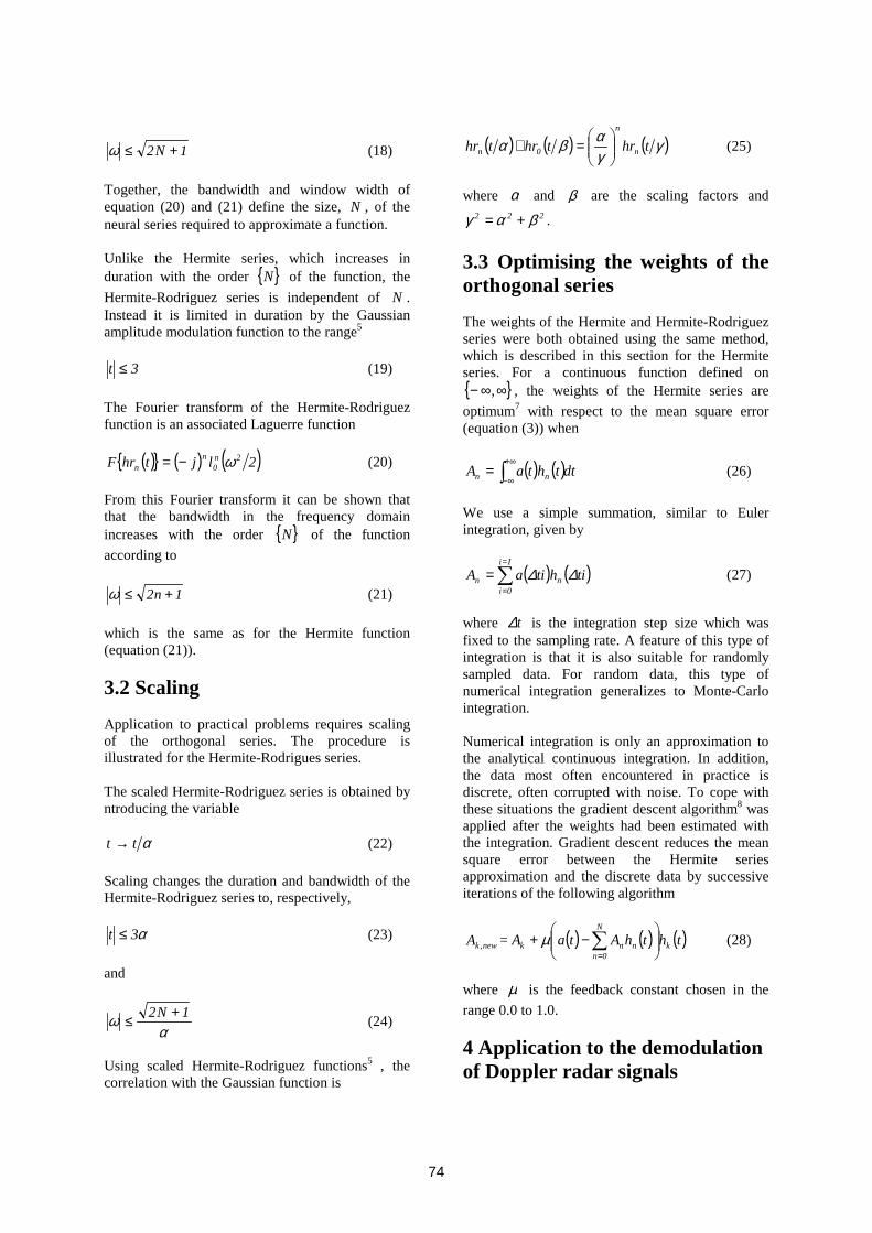
74

1N2 +≤ω (18)

Together, the bandwidth and window width of equation (20) and (21) define the size, N , of the neural series required to approximate a function. Unlike the Hermite series, which increases in duration with the order N of the function, the Hermite-Rodriguez series is independent of N . Instead it is limited in duration by the Gaussian amplitude modulation function to the range5

3t ≤ (19) The Fourier transform of the Hermite-Rodriguez function is an associated Laguerre function

( ) ( ) ( )2ljthrF 2n0

nn ω−= (20)

From this Fourier transform it can be shown that that the bandwidth in the frequency domain increases with the order N of the function according to

1n2 +≤ω (21) which is the same as for the Hermite function (equation (21)). 3.2 Scaling Application to practical problems requires scaling of the orthogonal series. The procedure is illustrated for the Hermite-Rodrigues series. The scaled Hermite-Rodriguez series is obtained by ntroducing the variable

αtt → (22) Scaling changes the duration and bandwidth of the Hermite-Rodriguez series to, respectively,

α3t ≤ (23) and

αω 1N2 +≤ (24)

Using scaled Hermite-Rodriguez functions5 , the correlation with the Gaussian function is

( ) ( ) ( )γγαβα thrthrthr n

n

0n

=∗ (25)

where α and β are the scaling factors and

222 βαγ += . 3.3 Optimising the weights of the orthogonal series The weights of the Hermite and Hermite-Rodriguez series were both obtained using the same method, which is described in this section for the Hermite series. For a continuous function defined on ∞∞− , , the weights of the Hermite series are optimum7 with respect to the mean square error (equation (3)) when

( ) ( )dtthtaA nn ∫+∞

∞−= (26)

We use a simple summation, similar to Euler integration, given by

( ) ( )∑=

==

Ii

0inn tihtiaA ∆∆ (27)

where t∆ is the integration step size which was fixed to the sampling rate. A feature of this type of integration is that it is also suitable for randomly sampled data. For random data, this type of numerical integration generalizes to Monte-Carlo integration. Numerical integration is only an approximation to the analytical continuous integration. In addition, the data most often encountered in practice is discrete, often corrupted with noise. To cope with these situations the gradient descent algorithm8 was applied after the weights had been estimated with the integration. Gradient descent reduces the mean square error between the Hermite series approximation and the discrete data by successive iterations of the following algorithm

newkA , = ( ) ( ) ( )ththAtaA k

N

0nnnk

−+ ∑

=

µ (28)

where µ is the feedback constant chosen in the range 0.0 to 1.0. 4 Application to the demodulation of Doppler radar signals

75

The objective of this section is to compare the performance of the Hermite with the Hermite-Rodriguez series on a practical signal processing problem. Figure 2(a) shows the signal received from the detector of a Doppler radar system. The carrier frequency, which is proportional to the velocity of the target, is removed by filtering to obtain the target range. The frequency spectrum of the Doppler signal, from which the velocity may be determined, is given by the new series formed by replacing the Hermite functions in the Hermite series interpolation of the Doppler signal by their Fourier transform (equation (9)). Removal of the carrier frequency to obtain the range of the target is achieved by taking the correlation of the Hermite series with the Gaussian function. The following mathematical model of a Doppler signal was investigated

( ) ( )( ) 22 2teft21ta σπ −+= cos (26) where the frequency, Hz1f = , and the Gaussian width, 03.=σ . Simulated random noise, with a uniform probability density, of varying strength was added. A Hermite series of 50 elements has a width of 010. seconds and a bandwidth of Hz51. , which is sufficient to accurately interpolate the Doppler signal. Figure 2(a), 2(b), and 2(c) show the signal, Gaussian filtered output and frequency spectrum respectively from the Hermite series interpolation containing 50 elements. The root mean square error (RMSE) of the Hermite series interpolation of the Doppler signal versus the number of Hermite functions in the series is shown in figure 3(a). For the purpose of comparison, the scaling parameters were chosen so that the Hermite-Rodriguez series matches the Hermite series. With

2=β , the order 0n = , Hermite-Rodriguez function is matched exactly to the order 0n = , Hermite function, that is ( ) ( )th2thr 00 = .

Similarly, with 2852.=α , the Hermite-Rodriguez series is matched in duration to the Hermite series. Figure 3(b), shows the root mean square error of the Hermite-Rodriguez interpolation as a function of the number of elements of the series. More than 400 Hermite-Rodriguez functions are needed before the error drops to a sufficiently small value. The reason for this is because the frequency response of the scaled Hermite-Rodriguez series is considerably smaller than a Hermite series of the same duration. Figure 4(a) and 4(b) shows the frequency response of the

Hermite series and Hermite-Rodriguez series on a unit amplitude cosine with 50 and 400 Hermite-Rodriguez functions respectively. The poor frequency response is unavoidable because a sufficiently large α must be chosen to ensure the series has sufficient duration to interpolate the Doppler signal. Figure 5 shows the output signal to noise ratio of the Hermite series, 50N = , and the Hermite-Rodriguez series, 400N = , versus the input signal to noise ratio. Nearly identical signal to noise ratios are achieved, which is to be expected since an identical Gaussian correlation function was used, but the Hermite series is considerably more efficient since it achieves the same result with much fewer terms in the series. In view of their Gaussian window, the Hermite-Rodriguez series may prove more suitable for correctly analyzing the frequency spectrum of signals subject to glitches. Conclusion A Gaussian filter using Hermite functions was developed. A comparison with a similar filter using the Hermite-Rodriguez series favours the Hermite series because it has a greater bandwidth for a series with the same number of elements. A comparison of the Hermite Gaussian filter with a Gaussian filter using Fourier functions is under investiagtion. References (1) G. Arfken, Mathematical methods for physicists, 2nd edition, Academic Press, New York, 1970. (2) G. G. Walter, Wavelets and other orthogonal systems with applications, CRC Press, USA, 1994. (3) M. R. Mackenzie and A. K. Tieu, Hermite Correlation and Application, submitted to IEEE Signal Processing, Sept 2002. (4) C. Konstantopoulos, L. Mittag, and G. Sandri, Deconvolution of Gaussian filters and antidiffusion, J. Appl. Phys., vol. 68, no. 4, pp 1415-1420, 1990. (5) L. R. Lo Conte, R. Merletti, and G. V. Sandri, Hermite expansions of compact support waveforms: applications to myoelectric signals, IEEE Trans. Biomed. Eng., vol. 41, no. 12, pp. 1147-1159, 1995. (6) P. A. Lindsay, Introduction to quantum mechanics for electrical engineers, McGraw-Hill, New York, 1967. (7) E. Kreyszig, Advanced engineering mathematics, 7th edition, John Wiley and Sons, United States, 1993.

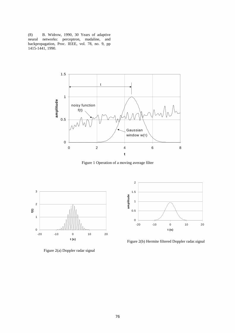
76

(8) B. Widrow, 1990, 30 Years of adaptive neural networks: perceptron, madaline, and backpropagation, Proc. IEEE, vol. 78, no. 9, pp 1415-1441, 1990.

0

0.5

1

1.5

0 2 4 6 8

t

ampl

itude

t

Gaussian window w(τ)

noisy function f(t)

Figure 1 Operation of a moving average filter

0

1

2

3

-20 -10 0 10 20

t (s)

f(t)

Figure 2(a) Doppler radar signal

0

0.5

1

1.5

2

-20 -10 0 10 20

t (s)

ampl

itude

Figure 2(b) Hermite filtered Doppler radar.signal

77

0

1

2

3

0 0.5 1 1.5

Frequency (Hz)

Pow

er

Figure 2(c) Power spectrum of Doppler radar signal by Hermite series.

0

1

2

3

4

5

6

7

0 10 20 30 40 50 60 70

number of Hermite functions

root

mea

n sq

uare

err

or

Figure 3(a) Root mean square error versus number of Hermite Functions.

0

1

2

3

4

5

6

7

0 100 200 300 400 500number of Hermite-Rodriguez functions

root

mea

n sq

uare

err

or

Figure 3(b) Root mean square error versus number of Hermite-Rodriguez functions.

-0.5

0

0.5

1

1.5

0 1 2 3Frequency

Am

plitu

de

Hermite (50)

Gaussian

Hermite-Rodriguez (50)

Figure 4(a) Frequency response of Hermite and Hermite-Rodriguez series with 50 elements.

-0.5

0

0.5

1

1.5

0 1 2 3Frequency

Am

plitu

deHermite (50)

Gaussian

Hermite-Rodriguez(400)

Figure 4(b) Frequency response of Hermite (50 elements) and Hermite-Rodriguez series (400

elements).

0.01

0.1

1

10

100

1000

0 1 2 3 4 5 6Input SNR

Out

put S

NR

Hermite

Hermite-Rodriguez

Figure 5 Comparative signal to noise ratios of Hermite and Hermite-Rodriguez Doppler radar

demodulator.

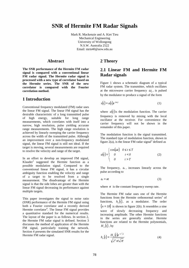
78

SNR of Hermite FM Radar Signals

Mark R. Mackenzie and A. Kiet Tieu Mechanical Engineering

University of Wollongong N.S.W. Australia 2522

Email: mrm40@uow.edu.au

Abstract The SNR performance of the Hermite FM radar signal is compared with a conventional linear FM radar signal. The Hermite radar signal is processed with a new type of correlator based on the Hermite series. The SNR of the new correlator is compared with the Fourier correlation method. 1 Introduction Conventional frequency modulated (FM) radar uses the linear FM signal. The linear FM signal has the desirable characteristic of a long transmitted pulse of high energy, suitable for long range measurements, which correlates with itself into a narrow, high resolution, pulse yielding accurate range measurements. The high range resolution is achieved by linearly sweeping the carrier frequency across the width of the transmitted pulse. Although an improvement over a non-frequency modulated signal, the linear FM signal is still not ideal. If the target is moving, several measurements are required to resolve the velocity and range of the target. In an effort to develop an improved FM signal, Klauder1 suggested the Hermite function as a possible modulation signal. Compared to the conventional linear FM signal, it has a circular ambiguity function enabling the velocity and range of a target to be resolved from a single measurement. The disadvantage of the Hermite signal is that the side lobes are greater than with the linear FM signal decreasing its performance against multiple targets. This paper investigates the signal to noise ratio (SNR) performance of the Hermite FM signal using both a Fourier correlator and a recently derived Hermite correlator4. The linear FM signal provides a quantitative standard for the numerical results. The layout of the paper is as follows. In section 2, the Hermite FM radar signal is defined. Section 3 discusses the method of application of the Hermite FM signal, particularly training the network. Section 4 presents the simulated SNR results for the Hermite FM radar signal.

2 Theory 2.1 Linear FM and Hermite FM Radar signals Figure 1 shows a schematic diagram of a typical FM radar system. The transmitter, which oscillates at the microwave carrier frequency oω , is pulsed by the modulator to produce a signal of the form

( ) ( ) tj oetats ω= (1) where ( )ta is the modulation function. The carrier frequency is removed by mixing with the local oscillator at the receiver. For convenience the carrier frequency will not be shown in the remainder of this paper. The modulation function is the signal transmitted. The standard type of modulation function, shown in figure 2(a), is the linear FM radar signal2 defined as

( )( )

><

≤≤=

Tt00t0

Tt0tta

ωcos (2)

The frequency, ω , increases linearly across the pulse according to

tκω = (3) where κ is the constant frequency sweep rate. The Hermite FM radar uses one of the Hermite functions from the Hermite orthonormal series3 of functions, ( )thn , as a modulator. The order 18n = is shown in figure 2(b). It resembles a sine wave of slowly decreasing frequency and increasing amplitude. The other Hermite functions in the series are generally similar. Hermite functions are related to the Hermite polynomials,

( )tH n , by

( ) ( )π!n2

etHth

n

2tn

n

2−

= (4)

79

where one of the many possible explicit forms of the Hermite polynomials is the derivative of the Gaussian function

( ) ( ) ( )22 tn

ntn

n edtde1tH −−= (5)

The optimum detector for the FM radar is the matched filter, which is equivalent to taking the cross-correlation between the transmitted and received signals. Defining ( )tb as the received signal then the output of the correlator detector is

( ) ( ) ( ) ( ) ( ) τττ dtbatbtatR +=∗= ∫+∞

∞− (6)

This integration may be evaluated digitally using a Fourier correlator. 2.2 Hermite FM detector In addition to the Fourier correlator, the Hermite FM radar signal can also be processed using a recently derived Hermite correlator4. The returned signal, ( )tb , is shifted in phase relative to the transmitted signal and corrupted with noise. It can be expanded in an orthogonal basis of Hermite functions defined to be

( ) ( )∑=

=N

0nnnh thBtb (7)

where the coefficients, nB , are a series of constants, often referred to as weights, which minimize the mean square error, mse, defined as

( ) ( )( )∫+∞

∞−−= dttbtbmse 2

h (8)

Using the Hermite orthogonal expansion for ( )tb , the correlation with the transmitted signal,

( ) ( )thta k= , is

( ) ( ) ( )∫+∞

∞−+= τττ dtbhtR hkh

( ) ( ) ∑ ∗=N

nnkn ththB (9)

where ( ) ( )thth nk ∗ is the correlation of two Hermite functions of different order, which is given by

( ) ( ) ( ) ( ) τττ dthhthth nknk ∫+∞

∞−+=∗ (10)

The solution to the Hermite correlation of equation (10) can be evaluated using Fourier transforms and shown to be an orthonormal associated Laguerre function4

( ) ( ) ( ) ( )( )

<≥−=∗

−

−+

0tfor2tl0tfor2tl1thth

2knk

2knk

kn

nk

and ( nk ≤ ) (11) where ( )tl n

k is the orthonormal associated Laguerre function5 , related to the associated Laguerre polynomials, ( )tLn

k , by

( ) ( )( ) !! kkn

tLettl

nk

2t2nnk

+=

−

(12)

Substituting into equation (9) we obtain the correlation as

( ) ( ) ( ) ( )∑∑=

−<

=

−+ +−=N

km

2kmkm

km

0m

2mkm

kmmh 2tlB2tl1BtR

for 0t ≥ (13) with a similar summation for 0t < . 2.3 Signal duration and bandwidth of Hermite functions The Hermite orthogonal expansion for ( )tb behaves as a window in the time domain. Outside this window it decays exponentially, limiting the effective range over which ( )tb may be approximated to within the window. The useful range of application of the Hermite expansion is then

1N2t +≤ (14) Where the right hand side, equal to the duration of the Hermite function of order N , may be determined via the Quantum mechanic solution of the Harmonic oscillator as the location where the oscillator energy becomes negative6. The Fourier transform operation on a Hermite function produces the same function (apart from a phase constant). Therefore a similar windowing effect occurs in the frequency domain and the useful bandwidth is

1N2 +≤ω (15) Together, the bandwidth and window width of equation (14) and (15) define the size, N , of the

80

Hermite expansion required to approximate a function. 3 Method 3.1 Recurrence relations for Hermite and Laguerre Functions Hermite and associated Laguerre functions are computed numerically by the following recurrence relations respectively5

( ) ( ) ( )1k

kth1k

2thtth 1kk1k +−

+⋅= −+ (16)

( ) =++

++ 1kn

1ktl n1k

( ) ( )tlk

kn1knktl

1kt1nk2 n

1knk −⋅+

++−⋅

+−++ (17)

with the initial values

( )

( )

=

=

−

−

2t1

2t40

2

2

e2

tth

e1th

π

π (18)

( )

( ) ( )( )

+⋅−+=

=

−

−

!

!

1nett1ntl

nettl

2t2nn1

2t2nn0

(19)

3.2 Hermite Expansion of the Received Signal For a continuous function defined on ∞−∞, , the weights of the Hermite expansion are optimum7 with respect to the mean square error (equation (3)) when

( ) ( )dtthtbB nn ∫+∞

∞−= (20)

This integration may be approximated numerically with Gauss-Jacobian integration8. Sometimes the scale and/or bias of the network are also optimized with back propagation or a similar algorithm9. The difficulty with the Gauss-Jacobian numerical integration is that the zeroes of the Hermite functions are required. For an order n Hermite function there are n zeroes. Consequently for a Hermite expansion consisting of a total of N

Hermite functions, the number of zeroes that must be found will be !N . In those applications, where only a few Hermite functions are required, this is acceptable but for large networks it places a heavy burden on computational speed and storage space. For this reason we use a simple summation, similar to Euler integration, given by

( ) ( )∑=

==

Ii

0inn tihtibB ∆∆ (21)

where t∆ is the integration step size which was fixed to the sampling rate. A feature of this type of integration is that it is also suitable for randomly sampled data. For random data, this type of numerical integration generalizes to Monte-Carlo integration. Although instability may occur in Euler integration, this has not been encountered in any of the applications so far investigated. Numerical integration is only an approximation to the analytical continuous integration. In addition, the data most often encountered in practice is discrete, often corrupted with noise. To cope with these situations the gradient descent algorithm was applied after the weights had been estimated with the integration. Gradient descent reduces the mean square error between the neural network approximation and the discrete data by successive iterations of the following algorithm

newkB , = ( ) ( ) ( )ththBtbB k

N

0nnnk

−+ ∑

=µ (22)

where µ is the feedback constant chosen in the range 0.0 to 1.0. In more elaborate training schemes, µ may be adaptively adjusted or adapted using directional minimization. 4 Results The Hermite function used for the transmitted/received signal was of order 18n = , as shown in figure 2(b). This signal has a duration

14t = seconds and the full width of the first peak of the correlated output is 80t .= seconds (figure 2(d)). Random noise, with a uniform probability density, of varying strength was added to the received Hermite signal. For the purpose of comparison, the linear FM radar signal power, frequency sweep rate and duration were carefully chosen to match the Hermite FM signal and also the width of the first peak of the correlated Hermite signal as closely as possible (figure 2(a) and 2(c)). The Fourier correlator consisted of two Fourier series expansions for the transmitted and received Hermite signals. Signal to noise ratios were evaluated on the correlated output of both radar

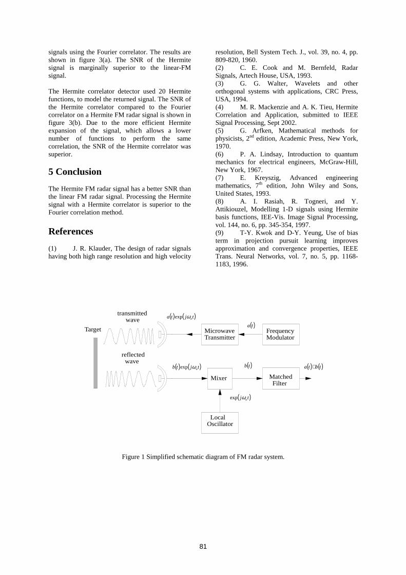
81

signals using the Fourier correlator. The results are shown in figure 3(a). The SNR of the Hermite signal is marginally superior to the linear-FM signal. The Hermite correlator detector used 20 Hermite functions, to model the returned signal. The SNR of the Hermite correlator compared to the Fourier correlator on a Hermite FM radar signal is shown in figure 3(b). Due to the more efficient Hermite expansion of the signal, which allows a lower number of functions to perform the same correlation, the SNR of the Hermite correlator was superior. 5 Conclusion The Hermite FM radar signal has a better SNR than the linear FM radar signal. Processing the Hermite signal with a Hermite correlator is superior to the Fourier correlation method. References (1) J. R. Klauder, The design of radar signals having both high range resolution and high velocity

resolution, Bell System Tech. J., vol. 39, no. 4, pp. 809-820, 1960. (2) C. E. Cook and M. Bernfeld, Radar Signals, Artech House, USA, 1993. (3) G. G. Walter, Wavelets and other orthogonal systems with applications, CRC Press, USA, 1994. (4) M. R. Mackenzie and A. K. Tieu, Hermite Correlation and Application, submitted to IEEE Signal Processing, Sept 2002. (5) G. Arfken, Mathematical methods for physicists, 2nd edition, Academic Press, New York, 1970. (6) P. A. Lindsay, Introduction to quantum mechanics for electrical engineers, McGraw-Hill, New York, 1967. (7) E. Kreyszig, Advanced engineering mathematics, 7th edition, John Wiley and Sons, United States, 1993. (8) A. I. Rasiah, R. Togneri, and Y. Attikiouzel, Modelling 1-D signals using Hermite basis functions, IEE-Vis. Image Signal Processing, vol. 144, no. 6, pp. 345-354, 1997. (9) T-Y. Kwok and D-Y. Yeung, Use of bias term in projection pursuit learning improves approximation and convergence properties, IEEE Trans. Neural Networks, vol. 7, no. 5, pp. 1168-1183, 1996.

transmitted wave

reflected wave

MicrowaveTransmitter

Mixer Matched Filter

( ) ( )tjta oωexp

FrequencyModulator

Target( )ta

( ) ( )tjtb oωexp ( ) ( )tbta ∗( )tb

LocalOscillator

( )tj oωexp

Figure 1 Simplified schematic diagram of FM radar system.

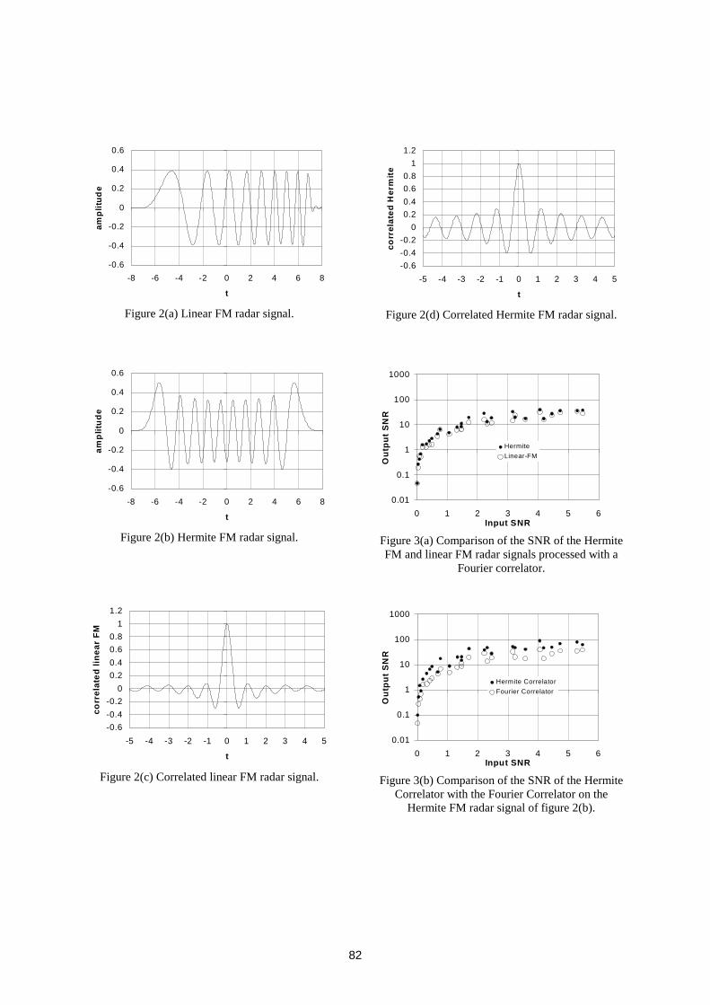
82

-0.6

-0.4

-0.2

0

0.2

0.4

0.6

-8 -6 -4 -2 0 2 4 6 8

t

ampl

itud

e

Figure 2(a) Linear FM radar signal.

-0.6

-0.4

-0.2

0

0.2

0.4

0.6

-8 -6 -4 -2 0 2 4 6 8

t

amp

litud

e

Figure 2(b) Hermite FM radar signal.

-0.6-0.4-0.2

00.20.40.60.8

11.2

-5 -4 -3 -2 -1 0 1 2 3 4 5

t

corr

elat

ed li

near

FM

Figure 2(c) Correlated linear FM radar signal.

-0.6-0.4-0.2

00.20.40.60.8

11.2

-5 -4 -3 -2 -1 0 1 2 3 4 5

t

corr

elat

ed H

erm

ite

Figure 2(d) Correlated Hermite FM radar signal.

0.01

0.1

1

10

100

1000

0 1 2 3 4 5 6Input SNR

Out

put S

NR

HermiteLinear-FM

Figure 3(a) Comparison of the SNR of the Hermite FM and linear FM radar signals processed with a

Fourier correlator.

0.01

0.1

1

10

100

1000

0 1 2 3 4 5 6Input SNR

Out

put S

NR

Hermite CorrelatorFourier Correlator

Figure 3(b) Comparison of the SNR of the Hermite

Correlator with the Fourier Correlator on the Hermite FM radar signal of figure 2(b).

! "# $%

&')(+* ',')(-/. 021 345'763*8 9 : ; < ; = ; >? @+A+B >+C > D @+EFEF= 9 < D G ; < @+9 :FH7> : > G+A D I

J)@ @+K >+A G ; < L >2H7> : > G+A D IJ)>+9 ; A >? @+AM7G ; >+C C < ; >FMON : P; >+E:

Q9 < L >+A : < ; N@ ?M7@+= ; IR/= : ; A G+C < GSTUG V/: @+9XW G+Y > : S MRZ [ \ Z

RQ7MOBHRW 8 R; G+9 ] G^ G+A >+Y _ `: K A < a C > L >+C : a = 9 < : Ga > b+=+a G+=

5')(7c 3de)d f)1 3O')(7c

J/< : D @FMON : ; >+E: SR)b >+C G+< b >S MRZ [ [RQ7MOBHRW 8 Rb G+9 < >+C ? `D < : D @a D @+E

gh i j k l m j n oOp q q r s t u p qOv w t x y zOu t x7w x u xO| w q zOu t xO r ~ w v p s t+w r| r s p /u q )p rOw q /p rOs p /p qu qUt x r q t r q r t rt p7t x ru q s r w y rp x u x| w q zOu t x/t w q y w t ~ w q t u s~ u q y p x u xO r ~ w y w t r ~ ~ u t r x p v y t x w y | r r q7 r s p q u y r t x w t p /ot pF r w s x!p v t u w ~Ov r p w q s rp r t x r y r/x u x| w q zOu t x r ~ w /v p s t+v w t x y t x r7 u ~ rt p)| rt w q y r r q r r y t px w r wOs r t w u qy u r q7t x u y v w v r z7r u q r y t u w t r t x rs p q q r s t u p q/| r t z7r r qt x r| w q zOu t xU r ~ w v p s t+w q )t x r u ~ ry u r p p v t u w ~ ot x p x v t w q u r p / ~ w y t pp | t w u q/t x r/u q u w ~ u ~ ry u rq r s r y y w / p w q ) u r q/| w q zOu t x r ~ w v p s t v w t x Xr y x p zUt x w t t x r r y u p qp o y r x w y w qOu /v p t w q t u /v w s t p qOt x u y /u q u w ~ u ~ r y u r zOx r qt x r+| w q zOu t x/ r ~ w 7v p s t u y r 7x u x/p + r 7~ p z w q t x w t t x r p y t s p /p q7o) r y u p q7 y r Ou qt p w y q t r q r tq r r yw) r /~ w rO u ~ rOt p)w s x u r r7w s s r v t w | ~ rv r p w q s rp r +x u x)| w q zOu t x/ r ~ w 7v p s t ~ u q y

O+O7++ ¡ ¢/ £ ¡ ¤ ¥ O

¦ §¨ ¨ ©7 ¤ ª ¥ ¤ « ¦O©Oª ¬+­ ® §­ ¤ £ ¡ O ¯ °­ O¯¨ F/ ¨ ± ¢ ¯¨ ¢ F¢ ¤ £­ ²¢ ³ ¥ ´ ¤ ¨ ° ­ 7¨ ¥ ¤ ³ ¢ ¨ ±U/ ¤ ¤ ¨ ­ µ ¦O©Oª¶ ¢ ²¯¨ ¢ U­ ¨ ±§ ¥ ¨ §·¨ ¢ ­ ¢ /¸7 ³ ¢¦ ¨ ­/¦¨ §)« ¸+¦¦¬ ® ¥ ¥ ¨ U ¢) ¨ ± + ¨ ³ ¢7 ¨ ­ ¨ § ´ ¤ ± ® ¨ ¤ ¨ ¹ ¨ ¢ ¢O® ¦O©OªU ) ¤ )® ³ ¤ ¤ £³ ¨ ¤ ¨ 7 ) ¡ ¨ ¤ ¤ 7 ¢ ¯¨ ¢ « º » ¼ ´ º ½ ¼ ¬ µ ¾/ ¯ ¡ ´ ³ ° ¯/¤ ¢ ± ´ ¡ ­ ¥ ¨ ® ¨ ¢¯/ ¿ ³ ® ® ¨ ¥ ¨ ¤ £7¤ ± À® ¨ ¤ ¨ ¹ ® +± ¨ ¡ ¢ ¯¨ ¢ ¢ ¤ £7­ ¢ ³ ¥ ¨ µ ¦ ¯ O ¨ Á ³ ¨ ¨ O ¥ £U U ¤ ¨ ¯/ ­ ® § ¥ //³ O¥  ­ ¥ ¨ ®O à / O ¥ §U­ ¤ ) ¢ ¯¨ ¢ ® ¨ §Ã ¤ ® ´ ¨ ¨ +¡ £/ ® ) 7¥ 7¨ ¯¨ ¤ + ¯ ° ¯/ / ÄFÅ©Æ­ ¥ ¤ ¨ ± )¥ ¨ X § ³ ® ¢ ¯¨ ¢ / / ¥ ¥ ¨ ¡ 7³ µ ¦ )¨ §U­ Á ³ ¨ ¯2 ¯ ¢Æ¨ ÇOÈ! ³ ¤ ¢Æ ƨ ¥ !¨ Æ¥ ¤ ¢ ¯¨ ¢ ³ § ¨ ¥ ¤ ¤ £/ ³ ¤ ¨ ¨ ¥ ¨ / ²­ +¤ £ ³ ± ­ ³ µ È!/ ¯%¨ U ¨ O­ ­ O + ¨ ¨ )¥ µÈ!O¯¨ ¤ ¤ ¢ ) ¨ £/® ¨ ¢ ¨ ¡ ¨ ±U ¤ £ ¨ ¥ ¤ ® §U³ ¤

® + ³ ± ­ ³ ® ¢ ¨ ® ® ¦O©Oª)¡ ¨ ´  ­ ² ¨ ±F ³ ± ­ ³ O¨ F §) ®7 ¢ ¯¨ ¢ 2¢ ¤ £F­ ¢ ³ ¥ ¢7® ¨ ¤ O ¨ ¹ O ¢7 )¥ ¤ ¥ ³ ¤ ¨ ± ¥ £® ¨ ¤ ¨ ¹ ) ¥ ¨ ¡ O 7 ­ ¨ § ¤ ³ ± ­ ³ ® 7¥ ¥ ¨ £³ ¨ ±2 U® §U³ ¤ µÉ+ U¯ °X­ ¢2¨ X ¨ ­ ­ ¯ ³ § U ¢ ¯¨ ¢ !¢ ¤ £X­ ¢ ³ ¥ 7 F ¥ ¯/ ¨ ¥ F§ F¥ ¥ ¨ X¥ Ê ¨ F

¤ ¡ F F­ ®/ 2 ¥ ¨ ¡ X¥ ¥ ¨ µO¦ F ³ ¤ ® ­ ¡ ¨ ³ ®/ ¨ ± ¤ )¥ ¥ ¨ £ ¨ ± U³ ¨ ¤ ¨ / ¨ / ¢ ¯¨ ¢ ¡ ¨ ¤ ¤ U ­ µ Ë¡ ³ ± ¨ ¨ O ) ¤ ¨ ¨ ¥ ³ §U­ ¨ ¨ ­ O7¯ +¥ ³ ­ ­ ³ ¢ §¨ ¨ § ¤ ® ¨ ¤ ¨ ¹ O® ¦O©Oª­ ® § ¥ 7 ¡ + ¨ ± ) ¢ ¯¨ ¢ )¢ ¤ £­ ¢ ³ ¥ ¤ ¨ ° µ¦ / / ¡ ¤+­ ­ 7¨ ¯/ ¨ ¥ ¤ £ ¨ ¥ ¤  ²

­ ¨ /® + ³ ± ­ ³ ®¢ ¨ ® ® ¦O©Oª+O¨ ± ¨ ¡ ´® ¥ ³ ¨ ±) )¢ ¨ ® ® ¯ °)¥ ¢ ¨ ¨ µ ¦ § Ê ¨ £ ® ­ ­ +® ¥ ³ + )¦O©Oª/ ³ ± ­ ³ ¯/ ¢ §¤ F¨ ­ « º Ì ¼ ´ º Í ¼ ´ º Î ¼ ´ º Ï ¼ ¬ µ ¦O©Oª ³ ± ­ ³ ¡ £ §U§ ¨ ¥¤ ¨ ° O¨ O¢ ¨ ¥ ³ ¢¨ ·º Ð ¼ ´ º Ñ ¼ ¢º Ò ¼ µ Ó ¤ £ / ³ 7 ®º Í ¼¥ ¨ ¢ /¨ §U­ ¥ ®O) ¨ ± ¢ ²¯¨ ¢ 2¢ ¤ £X­ ¢ ³ ¥ 7 X¦O©Oª2­ ® § ¥ µ+¦ § ¨ ¢ ¨ ® ® ¥ + ¯ ³ ¤ £ ¨ ¥ ¤ ­ ­ ¥ 7 ¢O +­ ²¡ ¨ ³ ¨ ´ ¯ ­ ¥ ¨ ¤ ¤ £¨ ¢O¨ 7 ¨ §²­ ¥ ¨ ¡ ¨ ³ ± ¨ ¨ ±/ ® ® O /¦O©Oª ³ ± ­ ³ µ ¦ ­ ¡ ¨ ³ ¤ £ ¨ ²¥ ¤ § ¢ ¤ +¢ ¨ ¢ ¤ £)¥ ¨ ¢ O ¢ £) ¡ ¨ ³ ®¦O©OªX¥ ¥ ¨ 7¨ ± ¨ ±U )¨ ¨ ¨ ¤+­ µ ¦ ¤ £7­ ­ ¨ ¥ ¤ ³ ¢ + § ³ ¢ £) ® O¨ ¨ ¨ ¤ ¨ ² ­ +¨ º » Ô ¼ µ ¾/ ¯ ¡ £) ¤ £7§ ¢ ¤ ¦O©Oª/¸7 ¢7 ³ § ¤ ¥ ¡ £7­ ® Õ ¤ ¯!Õ ¨ §7® + ¯ +¦O©OªU¡ ¨ µ È!  ­ ¤ ¨ ¥ ¨ ¤ £)§ ²¢ ¤ ¤ ¢ + ¨ ­ +® ¢ ¨ ® ® ¦O©Oª)¡ ¨ ¢ ¯ ¢/ ¨ O ³ §U­ ¨ U¨ + ¥ ¥ ³ µ¦ ¨ ­ ­ ¨ ± ¨ ¢7 ® ¤ ¤ ¯ Ç O  ¥ ¨

¯)¢ ¨ ¥ ³ ­ O ®¦O©OªF ® µ Õ ¥ ¨ 7 ¯ U¢ ¨ ¡ ¨ X ®O U ¤ £ ¨ ¥ ¤  ­ ¨ ® ¥ 7­ £7 O  §U­ ¤ ® ¦O©Oª)¦+ ´ ¤ ¢ ¢2 ¨ §U­ ¤ ®/ ¤ ¤7¦O©Oª¡ ¨ µ+¦ ¥ £X® ¨ ¤ ¨ ¹ ) ¥ ¨ ¡ ­ ¨ § ¤ ³ ± ­ ³ ¢ 7 ³ ¤ ² ¨ ¢ £/ ³ ® §U³ ¤ O­ ¢)¨ / ¥ ¨ / ÖOµ ¦ ¤ + ¥ ¨ U¥ ¥ ¤ ³ ¢ ­ ­ µ

× ØÙÚ Û+Ú)ÜÙ2++×)+ Ù77Ú Ü Û+Å Â §U­ ¤ 7® 7¦O©Oª¥ ¥ ¨ )¯¥ 7¦O©Oª

¦+ ¥ ³ ® §U³ ¤ 7  ­ ¨ ¡ ¨ ³ 7§ + ¨ §U­ ¤ µ É+¨ ± µ » µ ¯ )¥ ± ¨ )¯¨ ¢ ¯¢ ¡ ¤ ­ § ®O)¦O©OªF¦+ /¥ ¥ ¨ ¢ )¥ ² ­ ¢ ¨ ±7 ³ ® ® ¨ ¹ O )¨ § ¢ ¨ ³ µ Å!¦O©Oª¥ ¥ ¨ U O¨ )¨ ¨ ¨ ¤Õ ¤ ¯ÝÕ +­ 7¯/ ¨ ¥ ¨ U §U® ¡ £X¦O©Oª2¡ ¨ µ+¦ °2 ®Õ ¤ ¯Õ O¨ FÁ ³ ¨ ¥ ° ¤ £F­ U® ¡ ¨ ¤ ¤ U ¯ °F ¢ ²¯¨ ¢ / £  ­ ¨ ¤ ¤ £¨ ¥ ¨ ±/ ¥ ± ¨ )¯¨ ²

¢ ¯)µ ¦ ¨ ­ 7 ¢ ¯¨ /¥ ¨ ¢ ¤ ­ ¥ ° ¤ ²¥ ³ ¨ ¡ ¤ ¢ Æ ¡ ¨ ¤ ¤ Ý ³ ¥ ¢·¨ ® !® ¤ ¤ ¯ ¢Æ £ 2¦ ¨ UÞ F¸7 ¥ ¡ £­ ¯/ ¨ ¥ )¨ +¢ ¨ ® ® ® ¢ ¨ ® ® ¦O©Oª/¡ ¨ µ ¦ ¤ ­ )¨ O )Õ ¨ £Ó) ¥ ¨ ¤ ¤ £­ ¯/ ¨ ¥ U¨ §U® ) ¤ ¤7¸7 F ¢X¥ ± ¨ !¥ ¤7 ² ± ¨ + ¢¢ ¨ ® ® ® ¦O©Oª/¦+ µ É+ § ¢ ¨ ¤ ¢¢ ¥ ¨ ­ ¨ U ®¦O©OªF¥ ± ¨ U¥ ¤+ º » » ¼ µ

ß à á â ã â äå æ å ç è é êOå ë ì è í î ï ð ñï î ò è å ó è ë ë å ó ì à è ë

ô ô ô õ+ö7÷ö7ø ùOú+ô û ö7øUüUýþOÿ ø ! " ! # $ % % & ' & #

() * + , - , . / 0 / 1 20 - . 3 - 4 5 . 6 78 9 :9 ! ' # $ ; < =" >$$< ã " < ? # 9 % ì ò >$$@ A < ë B B ã #C A % ' " ! ' D " E 9 F9 GH ' G I F

JKL M N O P Q N RS T O ! % " # 9 A DU M"V OXWZY [ \ ] % ' " D ^ _ D >$$ " 9 `9 Q T a Y b JKL M N O P Q N RS T OcdZefWZg h iT P j j N g k lP >$$ #$ % ! m % I n o I p q ì ò >$$r Y sdmY ] dmY t u u udmY [ \ ] f Y [vZe # $ % ! % m

" >$$D 9 `9 Y w x y t z | ~ w x ] vZe # A D D ! D @ n JKL M N O P Q N RS T O " ' % $ $% %>" A # $ & % % ! % & 9 9 Y w x y t z t | ~ w x ] vZe@WEg h iT P j j N R #

%) 3 . + 6 , 7 + - 1 6 6 %7 1 7 3 %5 . 6 7 D: A ` $E$ ` f ` "$A # " & & 9 9 A m ;` ! _ @ @ E #$$ % % % " X ! % 9 9 % % ! & A # 8 9 X9

m E H ` YKL M N O P Q N RS T O A # A D D "9 Z9 ! ¡ n YKL M N O P Q N RS T O ! A Y w x y t z t | ~ w x ] vZe@WEg h iT P ¢ S h V N R Q T a Y b YKL M N O P Q N RS T OcdZefWZg h iT P ¢ S h V N g k lP>$$£ A H #¤$ Y w x y t z t | ~ w x ] vZe ! ' " % ! A 9 X9 # $ " X $ #

¥) 0 - . - , 1 + . 3 ¦6 , / / . - 1 3 %5 . 6 7$ $ A & & §¨ # 9 m9 &

; ' L M N O P Q N RS T O< # " A & @ n L M N O P Q N RS T O YKL M N O P Q N RS T O`dZe #©: ª « ¬ ­

YKL M N O P Q N RS T O`dZe ! " A X ' #8 : @9 G9 @ f$ f

Y w x y t z ~ w x ] vZe ! X : n Q T a Y b L M N O P Q N RS T OcdZe >$$ #:8 p" A ` " A % ! % & A # ! ¤ A qp £ ® YKL M N O P Q N RS T O`dZe #Z$ f ! X

L M N O P Q N RS T O:dEb L M N O P Q N RS T O`dZe cdEu u u ¯u u udEb YKL M N O P Q N RS T O:dZe c

' §°t | ~ w x ]± ² ]

k"v ° ~ w x \ ]± ² ]

k$ A ' A

° [± ² ]kW VDK b V;dZe c

Y$ % % ! " " A §

³KL M N O P Q N RS T O t dE´KL M N O P Q N RS T O:dEYY #

$ " " ! " g h iT P µ ¶ U Q P N R @WZY w x y t z ~ w x ] vZe_dZ¯ ¯

u u u ¯d ³KL M N O P Q N RS T O t dm´KL M N O P Q N RS T O:dmYY

$ " " " A " % § % L M N O P Q N RS T O ! ' >$$ # 9 " ! %>$$ & " ! % " A · ¸ ¹ U M"V OXWmL M N O P Q N RS T O% # º p ! e_d eL M N O P Q N RS T O >$$ e_d YL M N O P Q N RS T O >$$ % & % ! # $ % YKL M N O P Q N RS T O ! ! <>$$p o #Z I q YKL M N O P Q N RS T O`dZe ! " % ! %" ; # 9 %" & A e_dZeDd eL M N O P Q N RS T O dZeDd YL M N O P Q N RS T O dE¯ ¯

u u udZeDd L M N O P Q N RS T OL M N O P Q N RS T O dZeDd L M N O P Q N RS T O:dZeL M N O P Q N RS T O

& & L M N O P Q N RS T O:dmY@d ° ~ w x ]

± ² ]kL M N O P Q N RS T O

A b L M N O P Q N RS T O t dm³KL M N O P Q N RS T O:dmY

YKL M N O P Q N RS T O cd # ## # # L M N O P Q N RS T O:dmY

< >$$ " % $ % YKL M N O P Q N RS T O ! A _ _ #$ " " % " " A

g h iT P µ ¶ U Q P N g k lPWmQ T a Y b L M N O P Q N RS T OcdZu u u ¯# # # # dEb L M N O P Q N RS T O t dm³KL M N O P Q N RS T O:dmY

YKL M N O P Q N RS T O cdEu u u# # # d;L M N O P Q N RS T O:dm»

¼ ) ¥ _ 5 3 1 ½ ¾ 5 4½ - A " A $$ A &

# $ A U ¶ U Q P % A " " $ " g h iT P N g R¤W b g h iT P j j N R _dmg h iT P ¢ S h V N R _d

b g h iT P j j N g k lPDdmg h iT P ¢ S h V N g k lPDdu u u U ¶ U Q P Kg h iT P µ ¶ U Q P N R c"K¿:j jU ¶ U Q P Kg h iT P µ ¶ U Q P N g k lP c"KÀ¢¢

>$$ >" $% $ Áf9 9 Áf ' ;9 9 $ ! #

ô Â+õ Ã ô ø ÿÄ ô Å ÿÄ©@" " &A ! " § ©: % & % $ " " A ! A " Æ $ & § X " % Æ % & # $ ' $ E m A ` f E : A

lh Ç N g h iT P N g R¤W g h iT P µ ¶ U Q P N R K%¿:j jg h iT P µ ¶ U Q P N g k lPK%À¢¢ #

©@ " " " È ÉÊm ' E A #$ "A _ % % %$ #$ " A g h iT P N g R¤WZË ¯ ÌKlh Ç N g h iT P N g R #9 % @! @ % & f f _ % " " " A " & A ! & §Í k Q P j k Î PWb g h iT P j j N R _dmg h iT P ¢ S h V N R _dEu u u

u u ud U ¶ U Q P Kg h iT P µ ¶ U Q P N R cK¿:j j©@ $@>" $Ï >" $9 ! " " " $$ # 8 A % #

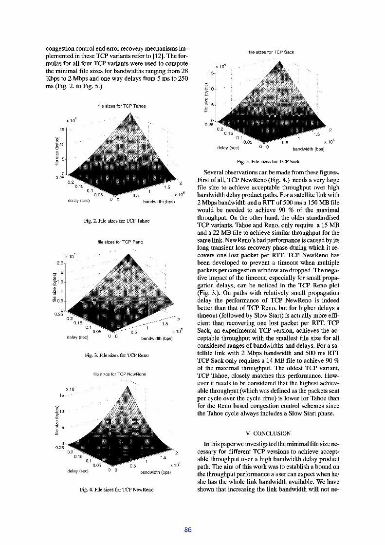
A & $A Ð ¨ < Ñ # $ & $A % % m< ÒÓ <ÁD " mÔ < Ô É # < # # Ô #

Õ Ö × Ø Ù Ø Õ Ö Ú Û Ü Ö Ý Û Ü Þ ß à á â ãá ä å ß Û

æ ç è é ê é æ ç ë ì í ç î ì í ï ð ñ ò ó ôõ ì ö ð

÷ ø ù ú û ú ÷ ø ü ý þ ø ÿ ý þ %ý ý

! " # $ % & ' " ! # ( ) % * ' + # *& -,.# / 10 " % ,2( 3 ' 10 ) 4 5 " ' 67 ) " ' ( % 01# $ $ 8 9:;=<> ?=@A * %CB 7 ) 4 6 D 6 EF* / '-#A! " GC$ # " 4 0 ) $ H' ) I .( %J# + 3 ) ! K# + + L ( # & $ .( 3 " % 5 4 3 L 5 (C% ! "C3 ) 4 3& # * / ?=) / ( 3C/ $ # GML " % / 5 + ( L # ( 3 ' 6 7 % " #' # ( $ $ ) ( $ ) * NA?=) ( 3OCPK& L '1& # * / ?=) / ( 3=# * /C#M@199K% 01Q R RM,.'#CS Q R>PJTK0 ) $ ?=% 5 $ /U& J* / /U( %V# + 3 ) ! XW RZY[% 0.( 3 J,.# \ ) ,.# $( 3 " % 5 4 3 L 5 ( 6 ]M*F( 3 >% ( 3 "3 # * / 8 ( 3 =% $ / "' ( # * / # " / ) ' /9:;.! # " ) # * ( ' 8 91# 3 % C# * /=@A * % 8 % * $ G=" ^ 5 ) " 2#=S Q=PJT# * />#MO O=PJTJ0 ) $ M( %># + 3 ) ! C' ) ,.) $ # "1( 3 " % 5 4 3 L 5 ( 0 % "1( 3 ' # ,. -$ ) * N 6 <> ?=@A * % _ ' & # /L " 0 % " ,.# * + ) ' + # 5 ' /& GA) ( '$ % * 4.( " # * ' ) * (-$ % ' 'A" + % ! " GFL 3 # ' =/ 5 " ) * 4=?>3 ) + 3H) (1" `+ % ! " 'F% * .$ % ' (ML # + N (AL "=@199-6-9:;2<> ?=@A * %K3 # '& *U/ ! $ % L /J( %JL " ! * (C#H( ) ,. % 5 (A?>3 *X,F5 $ ( ) L $ L # + N ( ' L " + % * 4 ' ( ) % *A?=) * / % ?2# " / " % L L / 6 93 -* 4 # `( ) ! C) ,FL # + (1% 0-( 3 M( ) ,. % 5 ( 8 ' L + ) # $ $ G>0 % "' ,.# $ $ L " % L # `4 # ( ) % *U/ $ # G ' 8A+ # *J& H* % ( ) + /J) *X( 3 .9:;V@A * %KL $ % (B 7 ) 4 6 a 6 E 6]M*JL # ( 3 'C?=) ( 3J" $ # ( ) ! $ GX' ,.# $ $AL " % L # 4 # ( ) % */ $ # G2( 3 XL " 0 % " ,.# * + X% 0.9:;Z<> ?=@A * %V) 'H) * / /& ( ( "( 3 # *.( 3 # (% 09:;J@A * % 8 & 5 (-0 % "3 ) 4 3 "M/ $ # G 'M#( ) ,. % 5 ( B 0 % $ $ % ?= /C& G= $ % ?V ( # " ( E-) '-# + ( 5 # $ $ G>,.% " A 0 0 ) `+ ) * (A( 3 # *J" + % ! " ) * 4X% * .$ % ' (AL # + N (AL "=@199-6-9:; # + N 8-# *K \ L " ) ,. * ( # $9:;J! " ' ) % * 8-# + 3 ) ! 'M( 3 F# + `+ L ( # & $ >( 3 " % 5 4 3 L 5 (1?=) ( 3H( 3 =' ,.# $ $ ' (0 ) $ =' ) I =0 % "A# $ $+ % * ' ) / " />" # * 4 '% 0-& # * / ?=) / ( 3 '# * /=/ $ # G ' 6 7 % "#M' # `( $ $ ) ( F$ ) * NH?=) ( 3JOKPK& L 'M& # * / ?=) / ( 3J# * /.Q R RH,.'C@1999:;H # + NF% * $ G=" ^ 5 ) " '#=S D=PJTX0 ) $ M( %=# + 3 ) ! >W RFY% 0C( 3 .,.# \ ) ,.# $A( 3 " % 5 4 3 L 5 ( 6-93 .% $ / ' (A9:;X! # " ) # * ( 89:;J91# 3 % 8-+ $ % ' $ GH,.# ( + 3 'M( 3 ) 'ML " 0 % " ,.# * + 6 b>% ?=` ! ") (1* / '( %=& C+ % * ' ) / " /=( 3 # ( ( 3 C3 ) 4 3 ' (1# + 3 ) ! `# & $ ( 3 " % 5 4 3 L 5 ( B ?>3 ) + 3M?=# '1/ 0 ) * /C# ' ( 3 L # + N ( '1' * (L "+ G + $ C% ! "( 3 C+ G + $ C( ) ,. E) '$ % ?= "-0 % "91# 3 % M( 3 # *0 % "A( 3 F@A * %.& # ' /H+ % * 4 ' ( ) % *H+ % * ( " % $' + 3 ,. 'M' ) * + ( 3 M91# 3 % C+ G + $ C# $ ?=# G ') * + $ 5 / '#C $ % ?c ( # " ( L 3 # ' 6

d1ef-ghAf1i jAk l ghm *( 3 ) ' L # L " ?= ) * ! ' ( ) 4 # ( /( 3 -,.) * ) ,.# $ 0 ) $ ' ) I 1* `+ ' ' # " G.0 % "M/ ) 0 0 " * (-9:;J! " ' ) % * 'A( %H# + 3 ) ! =# + + L ( `# & $ >( 3 " % 5 4 3 L 5 (% ! "A#>3 ) 4 3.& # * / ?=) / ( 3H/ $ # G.L " % / 5 + (L # ( 3 6 93 M# ) ,n% 01( 3 ) '1?=% " NC?=# '1( %> ' ( # & $ ) ' 3>#A& % 5 * /C% *( 3 ( 3 " % 5 4 3 L 5 ( L " 0 % " ,.# * + #5 ' " + # *M \ L + ( ?>3 *A3 o' 3 >3 # 'A( 3 C?>3 % $ >$ ) * N.& # * / ?=) / ( 3H# ! # ) $ # & $ 6 pX C3 # ! ' 3 % ?>*F( 3 # (-) * + " # ' ) * 4F( 3 C$ ) * N.& # * / ?=) / ( 3=?=) $ $-* % (1* `

+ ' ' # " ) $ G>" ' 5 $ ( ) *=# *=) * + " # ' M) *>( 3 M% & ' " ! /M( 3 " % 5 4 3 `L 5 ( 693 F) * ! ' ( ) 4 # ( ) % *H3 # 'M& *K+ # " " ) /H% 5 (& GH/ " ) ! ) * 4# * # $ G ( ) + # $ \ L " ' ' ) % * '-0 % "- # + 3=% 01( 3 A( 3 " L 3 # ' '% 01#9:;=( " # * ' 0 "1# * /M( 3 *C5 ' ) * 4C( 3 ' ( 3 " % 5 4 3 L 5 ( 0 % " ,F5 $ # '( %M+ % ,FL 5 ( ( 3 0 ) $ ' ) I * + ' ' # " GM( %M# + 3 ) ! # *M# + + L ( `# & $ C( 3 " % 5 4 3 L 5 ( 6 ]M5 "" ' 5 $ ( '3 # ! =' 3 % ?>*F( 3 # (-( 3 M?=# G( 3 U/ ) 0 0 " * (=9:;c! # " ) # * ( 'H" + % ! "F0 " % ,[( 3 X' ! " L # + N (1$ % ' ' 'A# ( ( 3 C& 4 ) * * ) * 4F% 0( 3 C+ % * * + ( ) % *F3 # '#' ) 4 * ) 0 ) + # * () ,FL # + (% *H( 3 =,.) * ) ,.# $0 ) $ F' ) I >* + ' ' # " G0 % "# + + L ( # & $ M( 3 " % 5 4 3 L 5 ( 69:;V<> ?=@A * % 8M% * J% 0=( 3 H* ?= ' (C9:;2! " ' ) % * ' 8?>3 ) + 3F?=# 'M/ ! $ % L /F( %FL " ! * (19:;J@A * % _ '( ) ,. % 5 (0 % "K,F5 $ ( ) L $ 2L # + N (.$ % ' ' 'JL "X+ % * 4 ' ( ) % *Z?=) * / % ?M8* / 'M& GH0 # "A( 3 =$ # " 4 ' (0 ) $ F' ) I >( %H% & ( # ) *H# + + L ( # & $ ( 3 " % 5 4 3 L 5 (-% ! "#C3 ) 4 3F& # * / ?=) / ( 3./ $ # G.L " % / 5 + (1$ ) * N 6]M$ / " 9:;C! " ' ) % * ' 8 $ ) N -91# 3 % % " @A * % 8 L " 0 % " ,2,F5 + 3& ( ( "K) *Z3 ) 4 3Z& # * / ?=) / ( 3Z/ $ # Gc * ! ) " % * ,. * ( ' 6M93 ) '' 3 % ?='( 3 # ( " ` ` * ( " ) * 4F $ % ?c ( # " (1+ # *=& M& * 0 ) + ) # $1) *' % ,. + # ' ' 6 ]M* $ GM0 % " $ % ?U& # * / ?=) / ( 3C/ $ # GML " % / 5 + ( ' ( 3 * 4 # ( ) ! J 0 0 + (>% 0F@A * % _ 'F( ) ,. % 5 (M?=# '.! ) ' ) & $ 69:; # + N 8 # '' L + ) 0 ) /C) *.q S O r 8 ) '# *> \ L " ) ,. * ( # $ 9:;=! " `' ) % *C( 3 # ( ) '1# & $ ( %A" # + 3># *C# + + L ( # & $ ( 3 " % 5 4 3 L 5 ( ?=) ( 3( 3 C' ,.# $ $ ' ( 0 ) $ C' ) I C% 0# $ $1) * ! ' ( ) 4 # ( />9:;.! " ' ) % * ' 6m (* / 'C( %H& .+ % * ' ) / " /H( 3 # (?= F% * $ GKL " ' * (( 3 + # ' .?>3 " K% * H9:;V+ % * * + ( ) % *U3 # '=( 3 H?>3 % $ H$ ) * N# ! # ) $ # & $ C# * />( " ) '( %>5 ( ) $ ) ' M( 3 C& # * / ?=) / ( 3F 0 0 ) + ) * ( $ G 6m *A" # $ ) ( GM) ( ) ' ,.% " -$ ) N $ GA( 3 # ( ,F5 $ ( ) L $ + % * * + ( ) % * ' ?=) $ $' 3 # " =#>$ ) * NF?>3 ) + 3F?=) $ $/ + " # ' >( 3 >& # * / ?=) / ( 3H/ $ # GL " % / 5 + ( 6 ]ML * ) * 4C# * /M+ $ % ' ) * 4C% 0 % ( 3 "1+ % * * + ( ) % * ' ?=) $ $# $ ' %A,.# N ( 3 & # * / ?=) / ( 3C/ $ # GML " % / 5 + ( ! # " ) # & $ / 5 " ) * 4( 3 M$ ) 0 ( ) ,. C% 0-( 3 C+ % * * + ( ) % *>?>3 ) $ A?= C3 # ! C# ' ' 5 ,. /) ( ( %C& M+ % * ' ( # * ( ) *=% 5 "1# * # $ G ' ' 6 m *>#?=# GC( 3 A" ' 5 $ ( '-) *% 5 "L # L "" L " ' * (-( 3 " 0 % " >( 3 M?=% " ' (+ # ' CL " 0 % " ,.`# * + C% 0-( 3 C/ ) ' + 5 ' ' />9:;.! # " ) # * ( ' 6

sMf-thAguHi v wAxy=v hz1k93 ) '=?=% " NX?=# '.+ # " " ) /U% 5 (M?=) ( 3U0 ) * # * + ) # $C' 5 L L % " (0 " % ,n( 3 C:A% ,F,.% * ?= # $ ( 3F% 01>5 ' ( " # $ ) #A( 3 " % 5 4 3=( 3 M:A% `% L " # ( ) ! C@A ' # " + 3F:A * ( " '; " % 4 " # ,H6

|1v v1|1v hAf1v1kq S r~PX6>$ $ ,.# * 8C:M6b># G ' 8Mb=6AM" 5 ' 8C16A]C' ( " `

,.# * * 8V 9:;[;1 " 0 % " ,.# * + ]M! " # ( $ $ ) ( ) * N ' 81; " % + / ) * 4 'C% 0A( 3 FQ ( 3 m * ( " * # ( ) % * # $:A% * 0 " * + >% *F91 $ + % ,F,F5 * ) + # ( ) % *. G ' ( ,.' 8PJ# " + 3 8~S W W 83 ( ( L1 o o ( + L ' # ( 6 $ " + 6 * # ' # 6 4 % ! o( + L ' # ( o L # L " ' 6 3 ( ,F$

q O r~:M6 ;1# " ( " ) / 4 8 9-6 6 3 L # " / 8 9:; o m ;>L " 0 % " ,.`# * + % ! "' # ( $ $ ) ( $ ) * N ' 8 m ` ` <> ( ?=% `" N 6 ! % $ 6 S S 8 * % 6 Q L ( 6 ` ` ]C+ ( 6 S W W L 6 D D ` ` W 6

q a rF6 M5 ,.# " 8 :A% ,FL # " # ( ) ! L " 0 % " ,.# * + A# * # $ G `' ) '-% 0 ! " ' ) % * '-% 0 9:;F) *>#$ % + # $ * ( ?=% " NM?=) ( 3#M$ % ' ' G>$ ) * N 8 m o =+ ,c9-" # * ' # + ( ) % * '% *><> ( `?=% " N ) * 4 8 ! % $ 6 8 * % 6 D 8 >5 4 6 S W W 8 L L 6 D Q ` ` W

q D r9-6 6 # N ' 3 ,.# * 81=61PJ# / 3 % ?M8 93 =L " 0 % " ,.`# * + M% 0-9:; o m ;F0 % "-* ( ?=% " N '1?=) ( 3=3 ) 4 3>& # * / `?=) / ( 3 ` ` / $ # GML " % / 5 + ( '1# * /A" # * / % ,V$ % ' ' 8 m o=+ ,9-" # * ' # + ( ) % * 'n% *<> ( ?=% " N ) * 4 8X! % $ 6 Q 8* % 6 a 8 5 * =S W W 8 L L 6 a a ` ` Q R

q Q r 6 ;1# / 3 G 816 7 ) " % ) 5 81=6 91% ?=' $ G 8- 61M5 " % ' 8 PJ% / $ ) * 4.9:;K( 3 " % 5 4 3 L 5 ( #F' ) ,FL $ >,.% / $# * /J) ( '= ,FL ) " ) + # $A! # $ ) / # ( ) % * 8Z=:APX6:A% ,.`L 5 ( "C:A% ,F,F5 * ) + # ( ) % *J@A ! ) ?M8! % $ 6 O 8-* % 6 D 8]C+ ( 6 S W W 8 L L 6 a R a ` ` S D

q r 7 6 PX6=>* 5 ,.8 6 91# ' ' ) 5 $ # ' 8H 7 5 * + ( ) % * ) * 4% 09:;>$ 4 % " ) ( 3 ,.'% ! "c#pU) " $ ' ' ) * N 8:A b>:<9@W W ` ` S RX:A * ( "C0 % "= # ( $ $ ) ( H# * /bCG & " ) /H:A% ,F,F5 * ) + # ( ) % *H<> ( ?=% " N 'A91 + 3 * ) + # $@A L % " ( 83 ( ( L1 o o ?C?C?C6 ) ' " 6 5 ,./ 6 / 5 o 91 + 3 @A `L % " ( ' o :A b>:<Mo 81S W W W

q r9-6 6 # N ' 3 ,.# * 8 =6 PJ# / 3 % ?M81TM6 5 ( " 8 9:; om ;U;1 " 0 % " ,.# * + F?=) ( 3X@A# * / % , % ' '=# * /JTA) `/ ) " + ( ) % * # $ :A% * 4 ' ( ) % * ' 8 m o =+ ,29-" # * ' # + `( ) % * 'J% *c<> ( ?=% " N ) * 4 8>! % $ 6 8=* % 6 Q 8=]C+ ( % & "O R R R 8 L L 6 Q D S ` ` Q Q D

q r9-6 6 # N ' 3 ,.# * 8 =6 PJ# / 3 % ?M81TM6 5 ( " 81 pU) * `/ % ?F` ` & # ' /X " " % ">" + % ! " GU# * /J0 $ % ?+ % * ( " % $?=) ( 3#c' $ % ?# + N * % ?>$ / 4 ,. * (J+ 3 # * * $ F#' ( 5 / G2% 0=9:; o m ;ZL " 0 % " ,.# * + 8 m < 7 ]C:A]CP_ W 6 93 :A% * 0 " * + % *C:A% ,FL 5 ( " :A% ,F,F5 * ) `+ # ( ) % * ' 8=! % $ 6 a 81S W W 8 L L 6 S S W W ` ` O R W

q W r~>6 b># ' 4 # ?=# 8 PX6 PK5 " # ( # 8 b=6 PJ) G # 3 # " # 8 ;1 " `0 % " ,.# * + M ! # $ 5 # ( ) % *=% 01bC99; o 9:;.% *=# ' G ,.`,. ( " ) +V* ( ?=% " N ' 8 m * ( " * # ( ) % * # $H % 5 " * # $K% 0:A% ,F,F5 * ) + # ( ) % *F G ' ( ,.' 8 ! % $ 6 S O 8 * % 6 D 8 5 $ G ` `>5 4 6 S W W W 8 L L 6 O S ` ` W 6

q S R r<=6-:A# " / ?= $ $ 816- # ! # 4 819-6 >* / " ' % * 8- PJ% `/ $ ) * 4H9:;J$ # ( * + G 81; " % + / ) * 4 ' m 2m <>`7 ]C:A]CPO R R R 8U:A% * 0 " * + % *:A% ,FL 5 ( ":A% ,F,F5 * ) + # ( ) % * ' 8 m 6F;1# " (J! % $ 6 a 8HO R R R 8L L 6 S D O ` ` Q1S

q S S r6K # + % & ' % * 8X :A% * 4 ' ( ) % *A! % ) / # * + # * /:A% * ( " % $ 8 :A% ,FL 5 ( " :A% ,F,F5 * ) + # ( ) % *M@A ! ) ?M8! % $ 6KS 8.* % 6.D 8.L L 6.a S D ` ` a O W 8.>5 4 6KS W 60 ( L1 o o 0 ( L 6 6 $ & $ 6 4 % ! o L # L " ' o + % * 4 # ! % ) / 6 L ' 6 A6

q S O r~16 7 $ % G / 8->6 7 # $ $ 8- ) ,F5 $ # ( ) % * ` ` & # ' /H:A% ,FL # `" ) ' % * 'X% 0K91# 3 % 8F@A * % 8F# * /n =:A9:;1 8:A% ,FL 5 ( "A:A% ,F,F5 * ) + # ( ) % *H@A ! ) ?M8 6 O =<=6a 8 5 $ GHS W W 8 L L 6 Q ` ` O S I

!" # %$&"'(

)+* , - */.0* , 12 , 3 4 5 4 6 4 7"8 9 :;)+7 < 7 = 9 >!>!6 , 5 = * 4 5 9 , 3? 9 9 @ 7 : * 4 5 A 7/BC7 3 7 * : = D ? 7 , 4 : 7"8 9 :0E * 4 7 < < 5 4 7/E F 3 4 7 >(3G/, 5 A 7 : 3 5 4 F!9 80E 9 6 4 DIHI6 3 4 : * < 5 *JK* LM3 9 ,!.0* N 7 3 ? * >!@ 6 3JK* LM3 9 ,!.0* N 7 3 O E HP Q R PHIGIE )%B0HM.02 H7 S S >(* 5 < T 4 * , - * UV5 7 7 7 W 9 : 1

XI* , 5 7 < Y < 9 : 7 * , 5? 5 3 = 9ME F 3 4 7 >(3Z [ \ ] .07 A 7 <+E * , 4 9 3%^%6 5 < _ 5 , 1HM_ 7 < * 5 _ 7 O E HP Q Q QHIGIE )%B0HM.02 H7 S S >(* 5 < T _ * , 5 7 < 8 UV= 5 3 = 9 W = 9 >

`acbMd e fMgMd2 ,!4 D 5 3%@ * @ 7 :;LM7I5 , A 7 3 4 5 1 * 4 7/4 D 7"@ 7 : 8 9 : >(* , = 7I9 8;) ?%hiI7 LMBC7 , 9!9 A 7 :0D 5 1 D(_ 7 < * F(* 3 F >!>(7 4 : 5 =/, 7 4 LM9 : N 3 W HI,7 j * >!@ < 7/8 9 :%3 6 = D(*/, 7 4 LM9 : N(= * ,!k 7I*I3 * 4 7 < < 5 4 7"k : 9 * _ S= * 3 4 8 9 : LM* : _C= D * , , 7 < * , _C*;>(9 _ 7 >l: 7 4 6 : ,/= D * , , 7 < W m73 4 6 _ 5 7 _%4 LM9%>(7 = D * , 5 3 >(3 4 9C= 9 @ 7+LM5 4 D"* 3 F >!>(7 4 : 5 =;, 7 4 SLM9 : N 3 T D 5 1 D < F!_ 7 < * F 7 _M* = N , 9 LI< 7 _ 1 >(7 , 4 30* , _M*C>(5 , 5 S>(* < : 7 4 6 : ,"k 6 8 8 7 : 3 5 n 7%9 8 9 , 7%* = N , 9 LI< 7 _ 1 >(7 , 4 @ * = N 7 4 W^C9 4 Do>(7 = D * , 5 3 >(3M* : 7(5 , A 7 3 4 5 1 * 4 7 _cLM5 4 Do6 , >(9 _ 5 8 5 7 _* , _I@ * = 7 _I) ?%h iI7 LMBC7 , 9 W p"6 :%5 , A 7 3 4 5 1 * 4 5 9 ,!3 D 9 LM7 _4 D * 4 @ * = 7 _I) ?%h LM5 4 D!*C>(5 , 5 >(* < : 7 4 6 : ,Ik 6 8 8 7 :03 5 n 7"9 k S4 * 5 , 3/4 D 7!D 5 1 D 7 3 4%4 D : 9 6 1 D @ 6 4C5 ,o4 D 7c3 4 6 _ 5 7 _o7 , A 5 : 9 , S>(7 , 4 W

qMrMs t d e ucvcwcgMd x u t);: * _ 5 4 5 9 , * < < FV= 9 , , 7 = 4 5 9 ,@ * 4 D 3!5 ,4 D 7o2 , 4 7 : , 7 4"D * A 7k 7 7 ,I8 * 5 : < FM3 F >!>(7 4 : 5 = * < O >(7 * , 5 , 1I4 D * 4 4 D 7Ck * , _ LM5 _ 4 D= * @ * = 5 4 FI8 9 :+4 D 7C8 9 : LM* : _I* , _I4 D 7C: 7 4 6 : ,M@ * 4 DM9 80*"= 9 , S, 7 = 4 5 9 ,CD * 3 k 7 7 ,C: 9 6 1 D < FC4 D 703 * >(7 W BC7 = 7 , 4 < F"*+, 6 >!k 7 :9 8C, 7 Ly, 7 4 LM9 : No* = = 7 3 3/4 7 = D , 9 < 9 1 5 7 3"D * A 7!k 7 7 ,c@ : 9 S@ 9 3 7 _I8 9 :;LID 5 = DM4 D 5 3C5 30, 9M< 9 , 1 7 :;4 D 7I= * 3 7 W z0j * >!@ < 7 39 8"4 D 7 3 7!4 7 = D , 9 < 9 1 5 7 3M* : 7 T;_ 5 : 7 = 4Ck : 9 * _ = * 3 4C3 * 4 7 < < 5 4 7 O* 3 F >!>(7 4 : 5 =c_ 5 1 5 4 * <"3 6 k 3 = : 5 k 7 :/< 9 9 @ 3 O0* , _K= * k < 7!>(9 S_ 7 >(3 | ~ O | Z ~ O | ~ O | [ ~ W )0D 7;>(* 5 ,C= D * : * = 4 7 : 5 3 4 5 =09 8 4 D 7 3 7, 7 Ly* = = 7 3 3C>(7 4 D 9 _ 3"5 3%4 D * 4;4 D 7/: 7 4 6 : ,c= D * , , 7 <+k * , _ SLM5 _ 4 DM= * ,Ik 7C>(* 1 , 5 4 6 _ 7 3%3 >(* < < 7 :+4 D * ,M4 D 7"9 , 7"8 9 :+4 D 78 9 : LM* : _M= D * , , 7 < W)0D 7;@ : 9 k < 7 >VLM5 4 DCk * , _ LM5 _ 4 D"* 3 F >!>(7 4 : F"5 3 4 D * 4 4 D 7;: 7 S4 6 : ,I= D * , , 7 < 5 3+, 9 4 * k < 7%4 9"D * , _ < 7%4 D 7%: * 4 7C9 8 : 7 4 6 : , 5 , 1* = N , 9 LI< 7 _ 1 >(7 , 4 3 W)0D 7 : 7 8 9 : 7 4 D 7 : 7 4 6 : ,= D * , , 7 <k 6 8 8 7 :+LM5 < <+3 4 * : 4 4 9Mk 6 5 < _I6 @(* , _I8 5 , * < < F(9 A 7 : 8 < 9 LLM5 < <9 = = 6 : O+: 7 3 6 < 4 5 , 1K5 ,o*!< 9 3 3/9 8/* = N , 9 LI< 7 _ 1 >(7 , 4 3 W )0D 5 3= : 7 * 4 7 3;4 LM9/@ : 9 k < 7 >(3;8 9 :;) ?%h @ 7 : 8 9 : >(* , = 7 W )0D 7C8 5 : 3 45 3 *;k 6 5 < _%6 @"5 ," 6 7 6 5 , 1/_ 7 < * F%LID 5 = D": 7 3 6 < 4 3 5 ,/* ,"5 , 8 < * S4 5 9 ,I9 8 4 D 7CBC9 6 , _");: 5 @/)05 >(7C B+)0)0+9 8 4 D 7%= 9 , , 7 = 4 5 9 , W)0D 5 3+5 , 8 < * 4 5 9 ,"9 8 B+)0)(= * 6 3 7 3+*0_ 7 = : 7 * 3 7%5 ,C4 D : 9 6 1 D @ 6 4 W)0D 7"3 7 = 9 , _/@ : 9 k < 7 >5 30*C: 7 _ 6 = 7 _/, 6 >!k 7 :09 8;* = N , 9 LMS< 7 _ 1 >(7 , 4l: 7 4 6 : , 5 , 14 94 D 73 7 , _ 7 : W)0D 5 3: 7 _ 6 = 7 _, 6 >!k 7 :09 80* = N , 9 LI< 7 _ 1 >(7 , 4 30@ 9 3 7 3C3 7 A 7 : * < @ : 9 k < 7 >(3

8 9 :;*C4 : * _ 5 4 5 9 , * < ) ?%h 3 7 , _ 7 : W )0D 7"5 , = : 7 * 3 7"9 8+4 D 7C= 9 , S1 7 3 4 5 9 ,oLM5 , _ 9 L5 3M_ 7 @ 7 , _ 7 , 4"9 ,K4 D 7!, 6 >!k 7 :I9 8/* = SN , 9 LI< 7 _ 1 >(7 , 4 3: 7 = 7 5 A 7 _ OK4 D 7y8 7 LM7 :* = N , 9 LI< 7 _ 1 S>(7 , 4 3C* : : 5 A 7 O 4 D 7I3 < 9 LM7 :04 D 7I= 9 , 1 7 3 4 5 9 ,MLM5 , _ 9 LLM5 < <1 : 9 Ly | ~ O | Z ~ O | P ~ W )0D 7M_ * 4 *M4 : * , 3 >(5 3 3 5 9 ,c5 3", 9 409 , < F3 < 9 LM7 _"_ 9 LI,"k F"4 D 70< 9 3 3 3+9 8 * = N , 9 LI< 7 _ 1 >(7 , 4 3 O 5 4 * < 3 9k 7 = 9 >(7 3 >(9 : 7;k 6 : 3 4 F W )0D 703 7 , _ 7 : 5 3 * < < 9 LM7 _%4 9"3 7 , _C* 3>(* , F/, 7 L_ * 4 *%@ * = N 7 4 3;* 3;9 < _/9 , 7 3;* : 7%* = N , 9 LI< 7 _ 1 7 _5 ,9 , 7Kk 6 : 3 4M5 , 4 9V4 D 7K, 7 4 LM9 : N W/2 , 4 7 : >(7 _ 5 * 4 7K: 9 6 4 7 : 6 7 6 7 3%>(5 1 D 4+, 9 4+k 7I* k < 7/4 9ID * , _ < 7/4 D 5 30k 6 : 3 4;9 80_ * 4 * | Z ~ O | ~ O | ~ W? 9 , 1 7 3 4 5 9 ,K= 9 , 4 : 9 <C5 3/, 9 4%4 D 7(9 , < Fo) ?%h >(7 = D * , 5 3 >5 >!@ * = 4 7 _!k F(k * , _ LM5 _ 4 Dc* 3 F >!>(7 4 : F W() ?%h0 3"7 : : 9 :0: 7 S= 9 A 7 : FI>(7 = D * , 5 3 >* < 3 9I_ 7 @ 7 , _ 3;9 ,I4 D 7%, 6 >!k 7 :;9 8 : 7 S4 6 : , 5 , 1I* = N , 9 LI< 7 _ 1 >(7 , 4 3 W Y+* 3 4 BC7 = 9 A 7 : F/: 7 4 : * , 3 >(5 4 3*!@ * = N 7 4%9 , = 7!4 D : 7 7!_ 6 @ < 5 = * 4 7(* = N , 9 LI< 7 _ 1 >(7 , 4 3/* : 7: 7 = 7 5 A 7 _ W 2 8 Y+* 3 4 BC7 = 9 A 7 : F"8 * 5 < 3;*04 5 >(7 9 6 4 5 3 , 7 = 7 3 3 * : F4 9I: 7 = 9 A 7 :;4 D 7"< 9 3 4 @ * = N 7 4+ | Z ~ O | [ ~ W2 ,"4 D 5 3 @ * @ 7 : LM7%5 , A 7 3 4 5 1 * 4 704 D 705 >!@ * = 4 4 D * 4 k * , _ LM5 _ 4 D* 3 F >!>(7 4 : F/D * 3;9 ,/4 D 7%@ 7 : 8 9 : >(* , = 7C9 8 ) ?%h iI7 LMBC7 , 9 | ~ O 4 D 7C, 7 LM7 3 4 ) ?%h A * : 5 * , 4 6 3 7 _I5 ,I4 9 _ * F 302 , 4 7 : , 7 4 Wm7V= 9 >!@ * : 74 D 7@ 7 : 8 9 : >(* , = 7V9 8(6 , >(9 _ 5 8 5 7 _l) ?%hiI7 LMBC7 , 9oLM5 4 DK) ?%h iI7 LMBC7 , 9K7 , D * , = 7 _oLM5 4 DKk F 4 7= 9 6 , 4 5 , 1* , _V@ * = 5 , 1 WC)0D 7 3 77 , D * , = 7 >(7 , 4 3o* : 7_ 7 S3 5 1 , 7 _K4 95 >!@ : 9 A 7() ?%h @ 7 : 8 9 : >(* , = 7!LID 7 ,4 D 7(8 : 7 S 6 7 , = F!9 80* = N , 9 LI< 7 _ 1 >(7 , 4 3%5 30: 7 _ 6 = 7 _ W)0D 7C, 7 j 4 3 7 = 4 5 9 ,M7 j @ < * 5 , 3+D 9 Lk * , _ LM5 _ 4 DI* 3 F >!>(7 4 : F5 >!@ * = 4 3() ?%h 4 D : 9 6 1 D @ 6 4 W"E 7 = 4 5 9 ,ll_ 7 3 = : 5 k 7 3!k F 4 7= 9 6 , 4 5 , 1C* , _%@ * = 5 , 1 W E 7 = 4 5 9 , [ @ : 7 3 7 , 4 3 4 D 7;3 5 >!6 < * 4 5 9 ,3 7 4 S S 6 @c* , _!@ * : * >(7 4 7 : 3C6 3 7 _!8 9 :%4 D 7!7 j @ 7 : 5 >(7 , 4 3"* , __ 5 3 = 6 3 3 7 3 4 D 709 k 4 * 5 , 7 _%: 7 3 6 < 4 3 W E 7 = 4 5 9 ,CP/= 9 , = < 6 _ 7 3 4 D 7@ * @ 7 : W

MrM f t vcyx vcd `bMMMd e Y+5 1 6 : 7M!3 D 9 LM3"4 D 7M, 7 4 LM9 : Nc>(9 _ 7 <%4 D * 4;LM* 3/6 3 7 _c5 ,4 D 5 3 LM9 : N W k LI 5 3+4 D 7%8 9 : LM* : _/ : 7 4 6 : , += D * , , 7 < k * , _ SLM5 _ 4 DC5 ,Ck 5 4 3 @ 7 : 3 7 = 9 , _ O JKE E"4 D 7+) ?%h JK* j 5 >!6 >lE 7 1 S>(7 , 4;E 5 n 7I5 ,!k F 4 7 3C* , _!* = N(5 3%4 D 7I3 5 n 7I9 8%* ,() ?%h * = SN , 9 LI< 7 _ 1 >(7 , 4+5 ,Mk F 4 7 3 W

forward buffer

bwf

bwr

mss

ack

ReceiverSender

return buffer

+ M "¡ ¢ £M¤ ¥M¦(¤ § ¨© ª ¤ «0 « ¬ ­ ®!¤ ¡M¯%°%©c¤ ª 0¬ « ± ¦!¦( ¢ ­"¨ ¡ ¥ «0® ¬ «« ® ¤ £I¡c¢ ® ¬ ¢0¯%°%©K¢ ® ¤ ® ² ¢%§ ¤ «"¡ ¤ ¢%§ ² ¡ §o¤ ¡c¢ ® ¬ £l³ ¬ ¡ § £M § ¢ ®I¬ « ± ¦!¦( ¢ ±(´ µ%¶

´ µ/· ¸³ ¢ ¬ ¢ ® +¤ ¡I¢ ® %¡ ¤ ¹

¦(¬ ¨ « §M¬ « ± ¦!¦( ¢ ±Mº ¬ ­ ¢ ¤ ;¥!» ¼ ½ ¾¸¼ ¿ ¾ À Á

¥! «%§ º ¡ §M¬ «  ÃÄÅ Æ ¶Ç+È È É ÊÅ Æ ·Ë Ì Í É ÊÎ º;¥(Ï+Ðo "¯%°%©!£M ¨ ¨ ³ ® ¬ ª /¬ «%¤ ª 0¬I« ± ¦!¦( ¢ ­"² ¬ ¢ ®

¸ « ² ­ ¢ ª ;¤ º ¢ ® ; ¬ £K³ ¬ ¡ § £M § ¢ ®"¬ « ± ¦!¦( ¢ ± Á ÑKª ¬ ¨ ¤ º+¥!Ï+Ðc " ¡ § ­ ¬ ¢ «;¢ ® ¬ ¢ ¢ ® C ¢ ¡I­ ® ¬ ¡ ¡ ¨ ­ ¬ ¡/® ¬ ¡ § ¨ ¢ ® c« ¢ ¬ ¦ ¤ º/ ¢ ¡ ¡ ¬ ­ ¥ ¡ ¤ £I¨ § ¦( ¡ ¢ « Á%Î º/¥lÒ ¯%°%©0Ó «M² º ¤ ¦(¬ ¡ ­ (£M ¨ ¨"³ o ¦!² ¬ ­ ¢ §K³ ±¢ ® c ¢ ¡­ ® ¬ ¡ ¡ ¨ ³ ¬ ¡ § £M § ¢ ®/¬ ¡ §C¢ ® ; ¢ ¡"³ º º « Ô %« ® ¤ £I¡" ¡¢ ® "º ¤ ¨ ¨ ¤ £M ¡ ! Õ ¬ ¦!² ¨ ÁÑM« « ¦((¬! ¢ ¡o³ º º "« Ô ( Ö ¬ ¨0¢ ¤c¢ ® M³ ¬ ¡ § £M § ¢ ®§ ¨ ¬ ±"² ¤ § ­ ¢ ¤ º ¢ ® %­ ¤ ¡ ¡ ­ ¢ ¤ ¡ Á ¯0® 0³ ¬ ¡ § £M § ¢ ®"§ ¨ ¬ ±² ¤ § ­ ¢ ¡I² ¬ ­ ¥ ¢ «0 «0§ º ¡ §I¬ «C´ µ%¶ ×+Ø!Ù0ÙÚlÛ Û ×CÜ

Á"+¤ 0¬C ¹¢ ¡"³ ¬ ¡ § £M § ¢ ®/¤ º ´ µ · ³ ¢ « ² « ­ ¤ ¡ §"¬ ¡ §"¬ ¡/¬ ­ ¥ ¡ ¤ £M¹¨ § ¦( ¡ ¢ « Ô %¤ º;Ý Þ Ã"³ ± ¢ «M ¢ ¢ ¬ ¥ « Ý Þ Ã ×CÜ´ µ/·

« ­ ¤ ¡ § « ¢ ¤¢ ¬ ¡ « ¦( ¢ ¤ ¡ C¬ ­ ¥ ¡ ¤ £I¨ § ¦( ¡ ¢ ÁCÎ º ¢ ® C¬ « ± ¦!¦( ¢ ±"º ¬ ­ ¹¢ ¤ ;¥! «0 ¬ ¢ 0¤ ¡

¸¢ ® " ¢ ¡!­ ® ¬ ¡ ¡ ¨+­ ¬ ¡ ¡ ¤ ¢ ® ¬ ¡ § ¨ ¢ ® %¬ ª ¬ ¨ ¬ ¢ %¤ º ¢ ® %¬ ­ ¥ ¡ ¤ £I¨ § ¦( ¡ ¢ « ¬ ¡ §C¢ ® ; ¢ ¡³ º º %£M ¨ ¨%³ !­ ¤ ¡ « ¢ ¬ ¡ ¢ ¨ ±oº ¨ ¨%¬ ¡ §o¤ ª º ¨ ¤ £M ¡ Á ¯0® «

¨ ¬ § «"¢ ¤c¬!Ö ¡ K§ ¨ ¬ ±o¤ ºM´ µ%¶ ×+Ø!Ù0ÙÚlÛ Û ×CÜ ×Ý Þ Ã ×CÜ´ µ/·

« ¹­ ¤ ¡ § «

¸£I® ­ ®K «I Ö ¬ ¨%¢ ¤c¥+ß à+¯0¯« ¡ ­ !¥K­ ¬ ¡o³ ( Õ ¹

² « « §M¬ « Âc´ µ%¶ × Ý Þ Ã ×CÜ´ µ/· × ÚlÛ Û ×"Ü

Á+¤ /¬(§ º º ¡ ¢% ¢ ¡o³ º º /« Ô !¢ ® (à+¯0¯l£M¤ ¨ §o¤ º­ ¤ « 0¡ ¤ ¢ ³ % ¡ ­ ¬ « §C³ ±"¢ ® 0º ¬ ­ ¢ ¤ ¥ Á áI¤ £M ª

¸ ¹« ² ­ ¢ ª I¤ º0¢ ® I¬ ­ ¢ ¬ ¨+ ¢ ¡!³ º º 0« Ô

¸¬ «%« ¤ ¤ ¡(¬ «0¥

Ò! 0¢ ® « ³ º º £M¤ ¨ §Cº ¨ ¨ ²/¬ ¡ §" ¦!² ¬ ­ ¢ ¢ ® %à+¯0¯o¤ º ¢ ® ­ ¤ ¡ ¡ ­ ¢ ¤ ¡!¤ ¡M¢ ® /« ¬ ¦("² ¡ ­ ² ¨ Á¯0® " ¡ ­ ¬ « C¤ º;à+¯0¯o¬ ¡ §/¢ ® %¨ ¤ « «0¤ º+¬ ­ ¥ ¡ ¤ £I¨ § ¦( ¡ ¢³ ¤ ¢ ®M­ ¬ « "¬"§ ­ ¬ « " ¡I¯%°%©(¢ ® ¤ ® ² ¢ ¬ ¡ §I¡ §/¢ ¤³ %² ª ¡ ¢ §"º ¤ ¯%°%©I¢ ¤C£M¤ ¥/ ¡I¬ « ± ¦!¦( ¢ ­% ¡ ª ¤ ¡ ¹¦( ¡ ¢ « Á+¯0® (¡ Õ ¢C« ­ ¢ ¤ ¡§ « ­ « « «I« ¤ ¨ ¢ ¤ ¡Kº ¤ "³ ¤ ¢ ®² ¤ ³ ¨ ¦(«âMãMäVåcæ çcè é åcêcë

ì/í îCíCï ð"ñ/ò óCôCõCóCöy÷!ø"ó/øIù ð"úyöIó/û ô%ü"õ¯0® %¬ 0¢ £M¤%£M¬ ± « ¢ ¤C § ­ 0¢ ® CÖ ¡ /§ ¨ ¬ ±I¤ º ¬ ­ ¹¥ ¡ ¤ £I¨ § ¦( ¡ ¢ « Á+ « ¢ «+¢ ¤" § ­ %¢ ® %¡ ¦!³ +¤ º+¬ ­ ¥ ¡ ¤ £I¨ § ¦( ¡ ¢ « ¡ ¢¬ «%² ¤ ² ¤ « §! ¡o¼ ý ¾0¬ ¡ §c¼ þ ¾ Á ÿ"¡ I¬ ­ ¥ ¡ ¤ £I¨ § ¦( ¡ ¢+ «« ¡ ¢ º ¤ ¬%­ ¢ ¬ ¡/¬ ¦(¤ ¡ ¢ ¤ º § ¬ ¢ ¬;² ¬ ­ ¥ ¢ ­ ª § Á ¯0® «¬ ¦(¤ ¡ ¢+¤ º0§ ¬ ¢ ¬"² ¬ ­ ¥ ¢+ «%§ ¡ ¤ ¢ §M¬ «0¢ ® Ý Ý Þ Ã µ Ý Þ ¢ ® ¤ ® ² ¢ ¢ ® «0² ¬ ² Á «0¢ £M¤Iº ¤ 0« ¢ ¬ ¡ § ¬ § « §I¯%°%©

¸³ ¢; ¢;­ ¬ ¡!³ ±M¦! ­ ®!® ® ;º ¤ % Õ ² ¦( ¡ ¢ ¬ ¨ ¢ ¬ ¡ « ² ¤ ¢² ¤ ¢ ¤ ­ ¤ ¨ « Á ¡ § ¡ !º £M %¬ ­ ¥ ¡ ¤ £I¨ § ¦( ¡ ¢ «C «C Ö ª ¬ ¨ ¡ ¢+¢ ¤I ¹§ ­ ¡ M¢ ® /« Ô /¤ º;¢ ® /¬ ­ ¥ ¡ ¤ £I¨ § ¦( ¡ ¢ «0¢ ¤ Ý Þ Ã ¬ ¡ §¢ ® º ¤ " § ­ «0¥!¬ ¡ §MÖ ¡ M¢ ¦( Á¯0® C« ­ ¤ ¡ §/« ¤ ¨ ¢ ¤ ¡I «+¢ ¤" § ­ %¢ ® % ¢ ¡/³ º º +« Ô ¢ ¤M¬"¦( ¡ ¦! ¦y¤ ºC "² ¬ ­ ¥ ¢ Á ¡ ­ "¢ ® " «0ª ¢ ¬ ¨ ¨ ±I¡ ¤ ¢ ¡(³ º º

¸¡ ¤(Ö ¡ c§ ¨ ¬ ±c¤ ­ ­ « Á ¯0® M º º ­ ¢; «¢ ® ¬ ¢; /¤ ¢ ¤ º;¥M¬ ­ ¥ ¡ ¤ £I¨ § ¦( ¡ ¢ «%¬ ª "¬ ¢ ¢ ® "« ¡ §

¸ º;¢ ® " ­ ª 0¬ ­ ¥ ¡ ¤ £I¨ § «% ª ±!§ ¬ ¢ ¬"² ¬ ­ ¥ ¢ Áì/í IíKñCðû óCöIúó/ðIõCõ%± ¢ I­ ¤ ¡ ¢ ¡ (» ¼ ¾

¸¼ ¾ À%¬ ¡ §M² ¬ ­ ¡ !» ¼ ¾

¸¼ ½ ¾ À%¬ /¬ ¨ ¹¢ ¬ ¢ ¤ ¡ «/¢ ¤c¢ ® !¯%°%©V« ¡ § "¢ ¤o­ ¤ ² M£M ¢ ®¬! § ­ §¡ ¦!³ ¤ º ¬ ­ ¥ ¡ ¤ £I¨ § ¦( ¡ ¢ « Á %± ¢ 0­ ¤ ¡ ¢ ¡ /¬ ¨ ¢ « ¢ ® £M¬ ±M¢ ® /­ ¤ ¡ « ¢ ¤ ¡I£M ¡ § ¤ £ «0 ¡ ­ ¬ « § Á Î ¢ ¡ ­ ¬ « «¢ ® I­ ¤ ¡ « ¢ ¤ ¡M£M ¡ § ¤ £³ ±!¢ ® I¬ ­ ¢ ¬ ¨;¬ ¦(¤ ¡ ¢;¤ º%§ ¬ ¢ ¬­ ¤ ª §³ ± ¬ ­ ®¬ ­ ¥ ¡ ¤ £I¨ § ¦( ¡ ¢K ¡ « ¢ ¬ §¤ º¢ ® ¡ ¦!³ 0¤ º0¬ ­ ¥ ¡ ¤ £I¨ § ¦( ¡ ¢ «; ­ ª § Á ¯0® «;² ª ¡ ¢ «¬"« ¨ ¤ £§ ¤ £I¡M¤ º;¢ ® "§ ¬ ¢ ¬"¢ ¬ ¡ « ¦( « « ¤ ¡/£I® ¡Mº £M ;¬ ­ ¹¥ ¡ ¤ £I¨ § ¦( ¡ ¢ «C¬ / ­ ª § Á ¯0® /¦(¬ ¡(§ ¬ £I³ ¬ ­ ¥!¤ º¢ ® «;« ­ ® ¦(C «;¬ ¡I ¡ ­ ¬ « C ¡/¢ ® %³ « ¢ ¡ « «;¤ º ¢ ® %§ ¬ ¢ ¬¢ ¬ ¡ « ¦( « « ¤ ¡

¸¬ ³ ¤ ª ¢ ® ³ « ¢ ¡ « « ¡ ­ §³ ±§ ¨ ¬ ± §K¬ ­ ¥ ¡ ¤ £I¨ § ¦( ¡ ¢ «M ¡K ¡ ¦(¤ § º §K¯%°%© Á;¯0® ³ « ¢ ¡ « «C «C­ ¬ « §M³ ±!¢ ® I ¡ ­ ¬ « §!¬ ¦(¤ ¡ ¢0¤ º%§ ¬ ¢ ¬² ¬ ­ ¥ ¢ «C¢ ® ¬ ¢;¢ ® M­ ¤ ¡ ¡ ­ ¢ ¤ ¡( «"¬ ¨ ¨ ¤ £M §M¢ ¤!¢ ¬ ¡ « ¦( ¢;¬ ¢¢ ® " ­ ² ¢+¤ º0¤ ¡ /¬ ­ ¥ ¡ ¤ £I¨ § ¦( ¡ ¢ Á

¯0® %ª ¬ ¬ ³ ¨ «;¬ % « §/¢ ¤/§ ­ § C¢ ® %¡ ¦!³ ;¤ º ¡ £§ ¬ ¢ ¬0² ¬ ­ ¥ ¢ « ¢ ¤"« ¡ §  ¯0® %­ ¤ ¡ « ¢ ¤ ¡C£M ¡ § ¤ £l» Þ µ À ¸£I® ­ ®( ª «C¢ ® M¬ ¦(¤ ¡ ¢0¤ º%¡ £² ¬ ­ ¥ ¢ «C¢ ® /¡ ¢ £M¤ ¥­ ¬ ¡V® ¬ ¡ § ¨ ¸¢ ® o¨ ¬ « ¢/² ¬ ­ ¥ ¢/¢ ¬ ¡ « ¦( ¢ ¢ §V» Ý ! " ! À

¸£I® ­ ®"« ² ­ º « º ¤ ¦£I® ;¢ ¤%« ¢ ¬ ¢¸¬ ¡ §0¢ ® ;¨ ¬ « ¢ ² ¬ ­ ¥ ¢¬ ­ ¥ ¡ ¤ £I¨ § § » #$ # ! " Ý Þ Ã À¸£I® ­ ®y ª «V¢ ® ¬ ¦(¤ ¡ ¢ ¤ º+² ¬ ­ ¥ ¢ «;¢ ® ¬ ¢ ® ¬ ª "¬ ¨ ¬ § ±I¨ º ¢ ¢ ® %¡ ¢ £M¤ ¥ Á

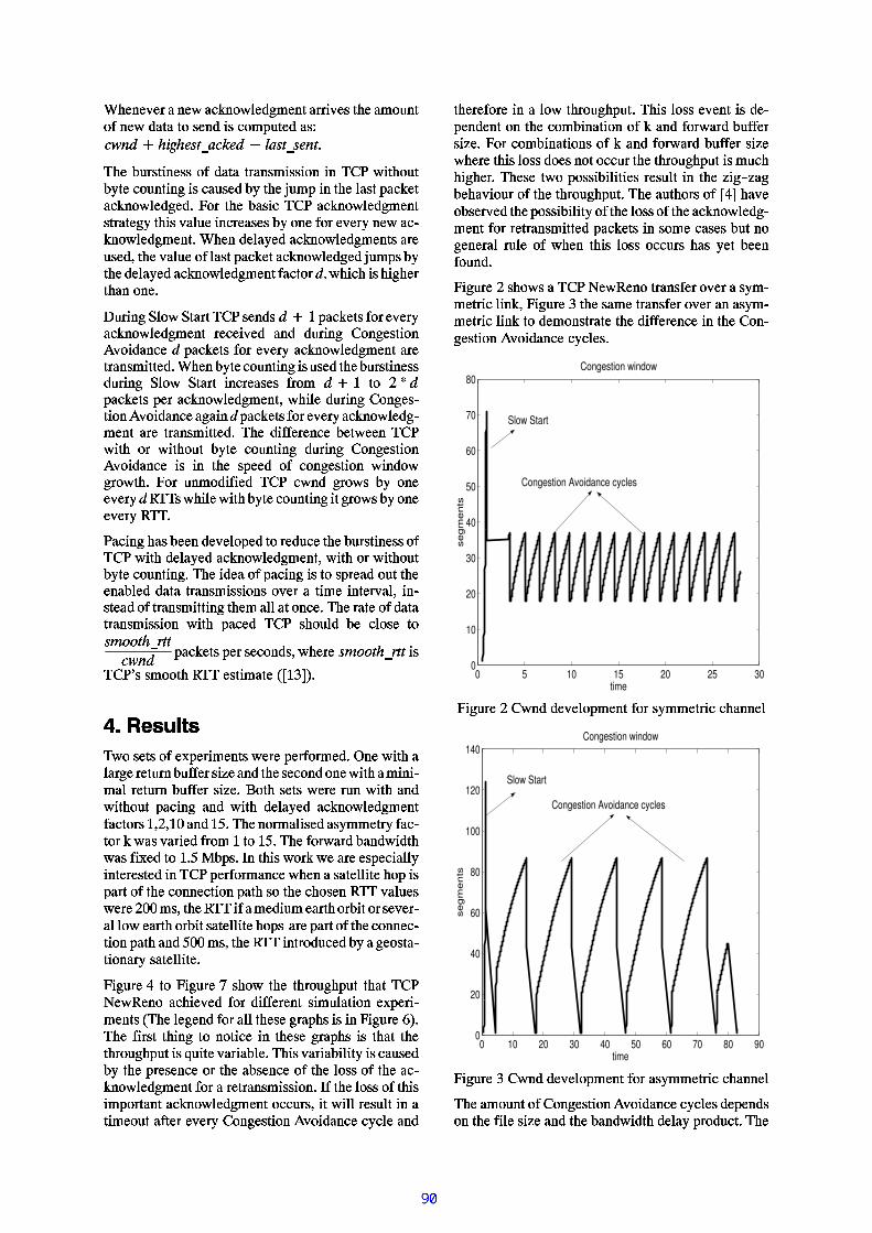
%l® ¡ ª ¬0¡ £l¬ ­ ¥ ¡ ¤ £I¨ § ¦( ¡ ¢ ¬ ª «+¢ ® %¬ ¦(¤ ¡ ¢¤ º;¡ £§ ¬ ¢ ¬"¢ ¤M« ¡ §M «%­ ¤ ¦!² ¢ §M¬ « ÂÞ µ '& #$ # ! " Ý Þ Ã )(* Ý ! " ! Á¯0® !³ « ¢ ¡ « «I¤ º/§ ¬ ¢ ¬!¢ ¬ ¡ « ¦( « « ¤ ¡o ¡o¯%°%©o£M ¢ ® ¤ ¢³ ± ¢ "­ ¤ ¡ ¢ ¡ I «0­ ¬ « §"³ ±I¢ ® + ¦!²M ¡/¢ ® C¨ ¬ « ¢ ² ¬ ­ ¥ ¢¬ ­ ¥ ¡ ¤ £I¨ § § Á++¤ /¢ ® !³ ¬ « ­(¯%°%©V¬ ­ ¥ ¡ ¤ £I¨ § ¦( ¡ ¢« ¢ ¬ ¢ ±/¢ ® «;ª ¬ ¨ C ¡ ­ ¬ « «;³ ±I¤ ¡ Cº ¤ + ª ±I¡ £¬ ­ ¹¥ ¡ ¤ £I¨ § ¦( ¡ ¢ Á %l® ¡!§ ¨ ¬ ± §M¬ ­ ¥ ¡ ¤ £I¨ § ¦( ¡ ¢ «0¬ « §¸¢ ® %ª ¬ ¨ C¤ º ¨ ¬ « ¢ ² ¬ ­ ¥ ¢ ¬ ­ ¥ ¡ ¤ £I¨ § §,+ ¦!² « ³ ±¢ ® 0§ ¨ ¬ ± §"¬ ­ ¥ ¡ ¤ £I¨ § ¦( ¡ ¢ º ¬ ­ ¢ ¤ -

¸£I® ­ ®/ « ® ® ¢ ® ¬ ¡!¤ ¡ Á

./ ¡ ¨ ¤ £ ¢ ¬ ¢ ¯%°%©M« ¡ § « '&0/ ² ¬ ­ ¥ ¢ « º ¤ ª ±¬ ­ ¥ ¡ ¤ £I¨ § ¦( ¡ ¢K ­ ª §¬ ¡ §§ ¡ °C¤ ¡ « ¢ ¤ ¡ÑCª ¤ § ¬ ¡ ­ 1-c² ¬ ­ ¥ ¢ «"º ¤ " ª ±o¬ ­ ¥ ¡ ¤ £I¨ § ¦( ¡ ¢0¬ ¢ ¬ ¡ « ¦( ¢ ¢ § Á %l® ¡C³ ± ¢ ;­ ¤ ¡ ¢ ¡ " « « §%¢ ® +³ « ¢ ¡ « «§ ¡ ¨ ¤ £ ¢ ¬ ¢c ¡ ­ ¬ « «Kº ¤ ¦ '&0/ ¢ ¤02 × ² ¬ ­ ¥ ¢ «"² "¬ ­ ¥ ¡ ¤ £I¨ § ¦( ¡ ¢¸£I® ¨ !§ ¡ o°C¤ ¡ « ¹¢ ¤ ¡%ÑCª ¤ § ¬ ¡ ­ 0¬ ¬ ¡-C² ¬ ­ ¥ ¢ « º ¤ ª ±C¬ ­ ¥ ¡ ¤ £I¨ § ¹¦( ¡ ¢/¬ c¢ ¬ ¡ « ¦( ¢ ¢ § Á0¯0® o§ º º ¡ ­ c³ ¢ £M ¡K¯%°%©£M ¢ ®¤ c£M ¢ ® ¤ ¢(³ ± ¢ ­ ¤ ¡ ¢ ¡ y§ ¡ °C¤ ¡ « ¢ ¤ ¡ÑCª ¤ § ¬ ¡ ­ « ¡¢ ® « ² §¤ ºK­ ¤ ¡ « ¢ ¤ ¡£M ¡ § ¤ £ ¤ £I¢ ® Á"+¤ ( ¡ ¦(¤ § º §l¯%°%©­ £I¡ §l ¤ £M«c³ ±¤ ¡ ª ±-"à+¯0¯+« £I® ¨ +£M ¢ ®C³ ± ¢ 0­ ¤ ¡ ¢ ¡ " ¢ ¤ £M« ³ ±"¤ ¡ ª ±!à+¯0¯;Á

©+¬ ­ ¡ /® ¬ «+³ ¡I§ ª ¨ ¤ ² §C¢ ¤" § ­ 0¢ ® %³ « ¢ ¡ « «+¤ º¯%°%©(£M ¢ ®(§ ¨ ¬ ± §!¬ ­ ¥ ¡ ¤ £I¨ § ¦( ¡ ¢¸£M ¢ ®(¤ ;£M ¢ ® ¤ ¢³ ± ¢ "­ ¤ ¡ ¢ ¡ Á ¯0® " § ¬"¤ º+² ¬ ­ ¡ M «;¢ ¤I« ² ¬ §M¤ ¢ ¢ ® ¡ ¬ ³ ¨ §o§ ¬ ¢ ¬!¢ ¬ ¡ « ¦( « « ¤ ¡ «I¤ ª /¬!¢ ¦(( ¡ ¢ ª ¬ ¨

¸ ¡ ¹« ¢ ¬ §"¤ º ¢ ¬ ¡ « ¦( ¢ ¢ ¡ "¢ ® ¦¬ ¨ ¨ ¬ ¢ ¤ ¡ ­ Á ¯0® 0 ¬ ¢ C¤ º § ¬ ¢ ¬¢ ¬ ¡ « ¦( « « ¤ ¡£M ¢ ®² ¬ ­ §¯%°%©« ® ¤ ¨ §³ ­ ¨ ¤ « l¢ ¤

! #" Þ µ

² ¬ ­ ¥ ¢ «+² +« ­ ¤ ¡ § «¸£I® ! #" «

¯%°%©0Ó «%« ¦(¤ ¤ ¢ ®!à+¯0¯ « ¢ ¦(¬ ¢ /» ¼ 3 ¾ À Á

4 ã15*6MëMçcæ è ë¯ £M¤I« ¢ «0¤ º0 Õ ² ¦( ¡ ¢ «+£M "² º ¤ ¦( § Á ÿ"¡ C£M ¢ ®M¬¨ ¬ ; ¢ ¡%³ º º « Ô ;¬ ¡ §%¢ ® ;« ­ ¤ ¡ §C¤ ¡ £M ¢ ®"¬+¦( ¡ ¹¦(¬ ¨% ¢ ¡o³ º º /« Ô ÁC¤ ¢ ®o« ¢ «"£M M ¡c£M ¢ ®o¬ ¡ §£M ¢ ® ¤ ¢I² ¬ ­ ¡ ¬ ¡ §£M ¢ ®§ ¨ ¬ ± §l¬ ­ ¥ ¡ ¤ £I¨ § ¦( ¡ ¢º ¬ ­ ¢ ¤ «;

¸½¸ þ"¬ ¡ §/ Á ¯0® ;¡ ¤ ¦(¬ ¨ « §"¬ « ± ¦!¦( ¢ ±Cº ¬ ­ ¹¢ ¤ ¥"£M¬ «+ª ¬ §"º ¤ ¦y %¢ ¤M Á ¯0® %º ¤ £M¬ §"³ ¬ ¡ § £M § ¢ ®£M¬ «;º Õ §/¢ ¤! Á 17o³ ² « Á Î ¡I¢ ® «+£M¤ ¥"£M"¬ C « ² ­ ¬ ¨ ¨ ± ¡ ¢ « ¢ §/ ¡/¯%°%©M² º ¤ ¦(¬ ¡ ­ 0£I® ¡I¬C« ¬ ¢ ¨ ¨ ¢ %® ¤ ²I «² ¬ ¢ ¤ º+¢ ® "­ ¤ ¡ ¡ ­ ¢ ¤ ¡I² ¬ ¢ ®M« ¤I¢ ® "­ ® ¤ « ¡!à+¯0¯oª ¬ ¨ «£M 0½ þ þ%¦(«¸¢ ® 0à+¯0¯( º ¬+¦( § ¦ ¬ ¢ ®C¤ ³ ¢ ¤ « ª ¹¬ ¨ ¨ ¤ £l ¬ ¢ ®/¤ ³ ¢ « ¬ ¢ ¨ ¨ ¢ 0® ¤ ² «I¬ 0² ¬ ¢ ¤ º ¢ ® 0­ ¤ ¡ ¡ ­ ¹¢ ¤ ¡"² ¬ ¢ ®/¬ ¡ § þ þC¦(«

¸¢ ® %à+¯0¯c ¡ ¢ ¤ § ­ §C³ ±/¬; ¤ « ¢ ¬ ¹¢ ¤ ¡ ¬ ±!« ¬ ¢ ¨ ¨ ¢ Á

+ /¿o¢ ¤o+ 8K« ® ¤ £¢ ® (¢ ® ¤ ® ² ¢C¢ ® ¬ ¢C¯%°%©9I £MàC ¡ ¤¬ ­ ® ª §Kº ¤ I§ º º ¡ ¢/« ¦! ¨ ¬ ¢ ¤ ¡ Õ ² ¹¦( ¡ ¢ «;» ¯0® %¨ ¡ §"º ¤ +¬ ¨ ¨ ¢ ® « % ¬ ² ® «; «0 ¡/+ À Á¯0® (º « ¢C¢ ® ¡ K¢ ¤o¡ ¤ ¢ ­ c ¡K¢ ® « ( ¬ ² ® «M «M¢ ® ¬ ¢C¢ ® ¢ ® ¤ ® ² ¢ «+Ö ¢ 0ª ¬ ¬ ³ ¨ Á ¯0® « ª ¬ ¬ ³ ¨ ¢ ±/ «+­ ¬ « §³ ±(¢ ® I² « ¡ ­ M¤ %¢ ® M¬ ³ « ¡ ­ M¤ º%¢ ® I¨ ¤ « «C¤ º%¢ ® I¬ ­ ¹¥ ¡ ¤ £I¨ § ¦( ¡ ¢ º ¤ ;¬C ¢ ¬ ¡ « ¦( « « ¤ ¡ Á Î º+¢ ® %¨ ¤ « «0¤ º ¢ ® « ¦!² ¤ ¢ ¬ ¡ ¢;¬ ­ ¥ ¡ ¤ £I¨ § ¦( ¡ ¢;¤ ­ ­ «

¸ ¢ £M ¨ ¨+ « ¨ ¢; ¡(¬¢ ¦( ¤ ¢;¬ º ¢ % ª ±(°C¤ ¡ « ¢ ¤ ¡IÑCª ¤ § ¬ ¡ ­ I­ ± ­ ¨ /¬ ¡ §

¢ ® º ¤ M ¡c¬I¨ ¤ £¢ ® ¤ ® ² ¢ Á ¯0® «C¨ ¤ « «" ª ¡ ¢0 «"§ ¹² ¡ § ¡ ¢0¤ ¡(¢ ® M­ ¤ ¦!³ ¡ ¬ ¢ ¤ ¡c¤ º%¥c¬ ¡ §!º ¤ £M¬ §M³ º º « Ô Á +¤ "­ ¤ ¦!³ ¡ ¬ ¢ ¤ ¡ «/¤ ºC¥K¬ ¡ §(º ¤ £M¬ §c³ º º "« Ô £I® %¢ ® «+¨ ¤ « «;§ ¤ «+¡ ¤ ¢ ¤ ­ ­ ¢ ® %¢ ® ¤ ® ² ¢ «+¦! ­ ®® ® Á ¯0® « !¢ £M¤(² ¤ « « ³ ¨ ¢ «/ « ¨ ¢% ¡o¢ ® MÔ ¹ ¹ Ô ¬ ³ ® ¬ ª ¤ 0¤ º;¢ ® "¢ ® ¤ ® ² ¢ Á ¯0® /¬ ¢ ® ¤ «%¤ º"¼ ¿ ¾+® ¬ ª ¤ ³ « ª §%¢ ® ;² ¤ « « ³ ¨ ¢ ±"¤ º ¢ ® 0¨ ¤ « « ¤ º ¢ ® 0¬ ­ ¥ ¡ ¤ £I¨ § ¹¦( ¡ ¢;º ¤ % ¢ ¬ ¡ « ¦( ¢ ¢ §!² ¬ ­ ¥ ¢ «" ¡c« ¤ ¦(M­ ¬ « «C³ ¢+¡ ¤ ¡ ¬ ¨" ¨ o¤ º/£I® ¡¢ ® «M¨ ¤ « «!¤ ­ ­ «M® ¬ «!± ¢"³ ¡º ¤ ¡ § Á+ /½I« ® ¤ £M«0¬C¯%°%©9I £MàC ¡ ¤/¢ ¬ ¡ « º +¤ ª ;¬C« ± ¦(¹¦( ¢ ­C¨ ¡ ¥

¸+ 3/¢ ® "« ¬ ¦(C¢ ¬ ¡ « º ;¤ ª 0¬ ¡M¬ « ± ¦(¹¦( ¢ ­"¨ ¡ ¥M¢ ¤M§ ¦(¤ ¡ « ¢ ¬ ¢ "¢ ® /§ º º ¡ ­ / ¡M¢ ® /°C¤ ¡ ¹ « ¢ ¤ ¡IÑCª ¤ § ¬ ¡ ­ /­ ± ­ ¨ « Á

0 5 10 15 20 25 300

10

20

30

40

50

60

70

80Congestion window

time

segm

ents

Slow Start

Congestion Avoidance cycles

:; < = > ?@1A,BDC E1E ? F ? G H I J? C K L H >,M N JJ? K > ; OO P Q C C ? G

0 10 20 30 40 50 60 70 80 900

20

40

60

80

100

120

140Congestion window

time

segm

ents

Slow Start

Congestion Avoidance cycles

RS T U V WX1Y,ZD[ \1\ W ] W ^ _ ` aW [ b c _ V,d e f aaW b V S gg h d [ [ W ^i,h Wd a_ U [ b _ cY_ [ T W e b S _ [j] _ S \ d [ g Wg f g ^ W e\ W ` W [ \ e_ [Db h Wc S ^ We S k Wd [ \b h Wl d [ \ Z1S \ b h1\ W ^ d fD` V _ \ U g b m i,h W

^ d V T W Vb h Wc S ^ We S k W_ Vb h We ad ^ ^ W V b h Wl d [ \ Z1S \ b hD\ W ^ d f` V _ \ U g b nb h W1a_ V WY_ [ T W e b S _ [j] _ S \ d [ g Wg f g ^ W ed V W[ W W \ W \ob _pb V d [ e c W VDb h WZDh _ ^ Wc S ^ W m,q cDb h Wl d [ \ Z1S \ b h\ W ^ d f*` V _ \ U g bS eph S T hrW [ _ U T h*b h d b[ _*Y_ [ T W e b S _ [j] _ S \ d [ g Wrg f g ^ WrS e)g _ a` ^ W b W \ nb h Ws] d V S d l S ^ S b f0S [b h V _ U T h ` U b,S eg d U e W \l fb h WD^ _ e e_ ctb h WDc S V e b,[ W Zud g vw [ _ ZD^ W \ T aW [ bd c b W V,S [ S b S d ^x ^ _ Zsx b d V b m

yDz z|~ Drt D~ uD ~q cb h WDV W b U V [l U c c W Ve S k WS e^ d V T W n_ ` b S ad ^b h V _ U T h ` U bg d [_ [ ^ fl W,d g h S W ] W \S c d g w [ _ ZD^ W \ T aW [ b e d V Wte W [ b e W ^ v\ _ a*W [ _ U T hb _` V W ] W [ b dt U W U Wtl U S ^ b U `Dd [ \_ ] W V c ^ _ Zmx W ^ \ _ auW [ _ U T h1aW d [ etb h d b b h WD\ W ^ d f W \1d g w [ _ ZD^ W \ T vaW [ b c d g b _ V \h d e b _l WT V W d b W V b h d [_ V W U d ^ b _ w n e S [ g Wb h W[ _ V ad ^ S e W \d e f aaW b V fc d g b _ V w T S ] W etb h Wh S T h W e bc V W U W [ g f_ ctd g w [ _ ZD^ W \ T aW [ b eb h d bb h WDV W b U V [g h d [ v[ W ^g d [e U ` ` _ V b mj1e ^ _ [ Td e \ w b h W V W,S e _ [ ^ fde ^ S T h b b h V _ U T h ` U b \ W T V d v\ d b S _ [l U b d ee _ _ [Dd e,d g w [ _ ZD^ W \ T aW [ b ed V We W [ b a_ V W_ c b W [b h d [_ [ W,c _ VW ] W V f w ` d g w W b e V W g W S ] W \ n b h Wt U W U We b d V b eb _l U S ^ \U `d [ \b h W,` W V c _ V ad [ g W\ W g V W d e W e m i,h S el W h d ] S _ U V S e a_ e b _ l ] S _ U e c _ V ` d g W \titYtDDW Z1W [ _S [RS T U V Wd [ \RS T U V W m i,h Wtad S [\ V d ZDl d g w _ c e W [ \ S [ Th S T h ^ f\ W ^ d f W \d g w [ _ ZD^ W \ T aW [ b eS eDb h W,[ W W \b _ w [ _ Zw S [_ V \ W V b _tl W,d l ^ Wb _g h _ e Wtd [S \ W d ^ \ W ^ d f W \d g w [ _ Z1v^ W \ T aW [ b c d g b _ V m

0 5 10 150

2

4

6

8

10

12

14

16

18x 10

4 TCP NewReno bwdel 70, rb70

k

Bp

s

D, ¡ ¢ £ ¤1 £ £ ¥ 1 £ ¦ §¨ © ¢1¡ ª ª t§¨ ©

«¢ £ ª £t¬t­®D ¤1¯ ¢ ª ,° ¤1 ¥ ¥ ¤1 ¥ s£ ¥ £* ¦ ± ¢ ¤D¥ £ ¢ pª p¡ ¢ £ ¤1 £ £ ¥ £ ¦ ª¨ © ¥ £D ¦ ¢ , ¦ £¡ D ª ¦ ¦ ¢ 1 ª ª , ¢ £ ª ² ¥ ¤'² ¤D ¥ , ¢ £ ª £tt¬t­D®D ¤1¯ ¢ ¡ ¥ t ¦ ª * ¥ ¥ ¥ ¤1 , t±D ª,³ © , t ¥ ª ±1§³ © ¦ ª ¦tª ª ´1D ¥ £ o £¢ ¢ ¥, ¥

¡ ¢tª ¢ £t t ¤D ¢¥ ª ¦ ± ¢ ¤D¥ £ ¢ ª , ¢ ¢D ¦ ¦ ,¡ ¢ £ ¤1 £ D£ ¥ µ£ ¦ ªt³ ¨ ¶1 ¢ £ ª £t¬t­®D ¤1¯ ¢ D ¤1 ¢ ¦ £t¬t­o®D ¤1¯ ¢ ¡ ¦ 1¡ ª ª D ª ² ¥ ¤·² «¢ £ ª £¸t¬t­s®D ¤1¯ ¢ ¤1 ¥ £ ¥ £o ¦ ± ¢ ¤D¥ £ ¢ D ± D p¥ ¢ D ¦ ª u

0 5 10 150

5

10

15x 10

4 TCP NewReno bwdel 175, rb 175

k

Bp

s

¹º » ¼ ½ ¾¿1À,Á ½  ¼ » Á à ¼ Ä Å ÆtÇ Æ È Éɾ Ä ½ È Ê Ë Ç Ì Í Î1º Í Ä ÁÍ ¾ Ï Ç È1à ½ Â Í ¼ Ð ÄÑpÒ Ó ¿ Ê ½ ¾ Ä ¼ ½ Ì1Ë ¼ Ô Ô ¾ ½tÑpÒ Ó ¿

Õ ÌÐ Â Ì Ð Ï ¼ Æ º  ̺ ÄÐ Ç Ì1Ë ¾DÆ Ç º ÍDÄ Á Ç ÄÇÏ Ç ½ » ¾½ ¾ Ä ¼ ½ Ì1Ë ¼ Ô Ô ¾ ½½ ¾ Æ ¼ Ï Ä Æ º ÌÅ ¾ ½ ȼ Ì Ã ½ ¾ Í º Ð Ä Ç Ë Ï ¾Ã ¾ ½ Ô Â ½ ÉÇ Ì Ð ¾Ô  ½ ¼ Ì ÉÂ Í º ÖÔ º ¾ Í ½ Ã Ç Ð ¾ ÍtÀt×tØÙD¾ Î1Ú¾ Ì Â,Î1º Ä ÁÇ Ï Ï Í ¾ Ï Ç È ¾ ÍtÇ Ð Û Ì Â Î1ÖÏ ¾ Í » ɾ Ì Ä Ô ½ ¾ Ü ¼ ¾ Ì Ð º ¾ Æ Ý

ÞDß àDßá*â ãDâ ä*åæçèté êDë ãuìDêí í èëÀ,Á ¾tÆ ¾ Ð Â Ì ÍtÎ1Ç ÈÄ Âà ½ ¾ Å ¾ Ì Ä Ü ¼ ¾ ¼ º Ì »Í ¾ Ï Ç Èº ÌÄ Á ¾½ ¾ Ä ¼ ½ ÌË ¼ Ô Ô ¾ ½º ÆÄ ÂpÐ Á Â Æ ¾Çɺ Ì º ÉÇ Ït½ ¾ Ä ¼ ½ ÌpË ¼ Ô Ô ¾ ½Æ º î ¾Â Ô1ÒÃ Ç Ð Û ¾ Ä Ý À,Á ¾1Ç Í Å Ç Ì Ä Ç » ¾1 ÔÇDɺ Ì º ÉÇ ÏË ¼ Ô Ô ¾ ½tÆ º î ¾1 ÔÒÃ Ç Ð Û ¾ Ä Ð Â ÉÃ Ç ½ ¾ Í,Ä ÂtÁ º » Á Ï ÈÍ ¾ Ï Ç È ¾ ÍÇ Ð Û Ì Â ÎDÏ ¾ Í » ɾ Ì Ä Æº Æ Ä Á Ç Ä Î1º Ä ÁÇË ¼ Ô Ô ¾ ½ Â Ô ÒÄ Á ¾Û Ö Ö Ò,Ç Ð Û Ì Â ÎDÏ ¾ Í » ɾ Ì Ä Æ Ä Á Ç ÄÐ Ç Ì Ì Â Ä Ë ¾,Æ ¼ à à  ½ Ä ¾ ÍË ÈÄ Á ¾,½ ¾ Ä ¼ ½ ÌÐ Á Ç Ì Ì ¾ Ï Ç ½ ¾,Í ½  à à ¾ ÍÇ ¼ Ä Â ÉÇ Ä º Ð Ç Ï Ï ÈÎ1º Ä Á  ¼ ľ ï Ã Ï º Ð º ÄtÛ Ì Â ÎDÏ ¾ Í » ¾Â ÔÛ Ý À,Á ¾Ë ¾ Ì ¾ Ô º Ä Æ ÔÇÆ ÉÇ Ï Ï ½ ¾ Ä ¼ ½ ÌË ¼ Ô Ô ¾ ½Æ º î ¾Â ÌDÀt×tØ1Ä Á ½  ¼ » Á Öà ¼ Ä Š¾ ½,Ç Æ È Éɾ Ä ½ º ÐÏ º Ì Û ÆÎ1¾ ½ ¾º Ì Å ¾ Æ Ä º » Ç Ä ¾ ÍDº Ìuð Ò ñ ò ÝóD Î1¾ Å ¾ ½Â Ì Ï ÈpÀt×tظھ Ì ÂÎ1º Ä ÁoÄ Á ¾Ç Ð Û Ö Ö ¾ Å ¾ ½ È Ö Ö Â Ä Á ¾ ½Ç Ð Û Ì Â ÎDÏ ¾ Í » ɾ Ì Ä Æ Ä ½ Ç Ä ¾ » ÈtÎ1Ç ÆÐ Â Ì Æ º Í ¾ ½ ¾ ͺ ÌÄ Á º Æ Î1 ½ ÛÇ Ì ÍÌ Âp¾ ï à ¾ ½ º ɾ Ì Ä ÆÎ1¾ ½ ¾Ã ¾ ½ Ô Â ½ ɾ ÍÄ ÂpÅ Ç Ï º Í Ç Ä ¾Ä Á ¾Ç Ì Ç Ï È Ä º Ð Ç Ï,½ ¾ Æ ¼ Ï Ä Æ ÝÀ,Á ¾Æ º ɼ Ï Ç Ä º  Ìo¾ ï à ¾ ½ º ɾ Ì Ä Æà ½ ¾ Æ Ö¾ Ì Ä ¾ ͺ ÌÄ Á º Æ Ã Ç Ã ¾ ½ Ð Â Ì Ô º ½ É)Ä Á Ç Ä Ç,Æ ÉÇ Ï Ï ¾ ½ ½ ¾ Ä ¼ ½ ÌË ¼ Ô Ô ¾ ½Æ º î ¾1½ ¾ Æ ¼ Ï Ä Æº ÌÁ º » Á ¾ ½Ä Á ½  ¼ » Á à ¼ Ä,Ô Â ½Àt×tØoÙD¾ Î1Ú¾ Ì ÂÎ1º Ä ÁÇ Ì ÍÎ1º Ä Á  ¼ ÄÃ Ç Ð º Ì »1À,Á ¾½ ¾ Æ ¼ Ï Ä Æt Ô,Ä Á ¾ Æ ¾Æ º ɼ Ï Ç ÖÄ º  Ì1¾ ï à ¾ ½ º ɾ Ì Ä Æ,Ç ½ ¾Æ Á  ÎD̺ ÌD¹º » ¼ ½ ¾ô1Ç Ì Í¹º » ¼ ½ ¾Ó ÝÀ,Á ¾Ç Í Å Ç Ì Ä Ç » ¾Â ÔÇɺ Ì º ÉÇ Ï Ë ¼ Ô Ô ¾ ½Æ º î ¾º Æ,Ð Ï ¾ Ç ½ Ï ÈÅ º Æ Öº Ë Ï ¾Ô  ½Ã Ç Ð ¾ ÍÀt×tظÙD¾ Î1Ú¾ Ì Â ÝÀ,Á ¾Ä Á ½  ¼ » Á à ¼ Ätà ¾ ½ ÖÔ Â ½ ÉÇ Ì Ð ¾º ÆtÇ Ï ÉÂ Æ Äº Ì Í ¾ à ¾ Ì Í ¾ Ì Ä Ô ½  ÉrÄ Á ¾Ç Æ È Éɾ Ä ½ ÈÔ Ç Ð Ä Â ½ Û Ê Ô Â ½ Ç Ï Ï Í ¾ Ï Ç È ¾ ÍÇ Ð Û Ì Â ÎDÏ ¾ Í » ɾ Ì Ä Ô ½ ¾ Ü ¼ ¾ Ì Ð º ¾ Æ Ýõ¸º Ä Á  ¼ Ä Ã Ç Ð º Ì »DÇtɺ Ì º ÉÇ Ï Ë ¼ Ô Ô ¾ ½Æ º î ¾º ÆË ¾ Ì ¾ Ô º Ð º Ç Ï Ô Â ½

Æ ÉÇ Ï Ï Í ¾ Ï Ç È ¾ ÍDÇ Ð Û Ì Â ÎDÏ ¾ Í » ɾ Ì Ä Ô ½ ¾ Ü ¼ ¾ Ì Ð º ¾ Ætö Í1ÑpÒ ½÷ ø Ý

0 5 10 150.8

0.9

1

1.1

1.2

1.3

1.4

1.5

1.6

1.7

1.8x 105 TCP NewReno, bwdel 70, rb 2

k

Bps

d=1,unmodd=2, unmodd=10, unmodd=15, unmodd=1, pacedd=2, pacedd=10, pacedd=15, paced

ùú û ü ý þÿ ý ü û ü þ ý 1ú þ ý ü ý þ ü ý ü þ ý

0 5 10 150.5

1

1.5x 10

5 TCP NewReno bwdel 175, rb2

k

Bp

s

! " # $&%'( # ) " ! ( * " + , -. - / 0 0$ + # / 1 2 . 3 4 5 4 + (4 $ 6 . /* # ) 4 " 7 +89 % : 1 # $ + " # 32 " ; ; $ #89

<&3 0) 4 ; $ 4'=>?4 ) $ -3 ) + * $ # ; ) # 0@5$ 6 6 5 + ( .&- 0. 6 62 " ; ; $ #- A $. 3 4 .&( ! (4 $ 6 . / $ 4. 7 B 3 ) 56 $ 4 ! 0$ 3 + ; . 7 C+ ) # D '( -E -E7 . " - $ 4 2 / + ( $ 3 7 # $ . - $ 46 ) - -F) ;4 " * 6 7 . + $. 7 B 3 ) 56 $ 4 ! 0$ 3 + -5 + ( .F0 3 0. 6 2 " ; ; $ #- A $ D G&" * 6 C7 . + $. 7 B 3 ) 56 $ 4 ! 0$ 3 + -H 4 " * . 7 B - I&. # $3 $ , $ #&4 $ 6 . / $ 42 " + - $ 3 + 0 0$ 4 . + $ 6 / D J ; + ( $# $ + " # 3F2 " ; ; $ # - 6 . # ! $+ ( $ - $4 " * . 7 B -E. # # , $$ , $ 3 + " . 6 6 /. + + ( $- $ 3 4 $ # 1 5 + (.F0 3 C0. 6 2 " ; ; $ # - A $0. 3 /&) ; + ( $ 0K. # $4 # ) * * $ 4 D > . 7 $ 4'=>L$ 5ME$ 3 )0) - + 6 /( . -0) # $F* . 7 B $ + - 3; 6 ! ( + + ( . 3" 3 C0) 4 ; $ 4'=>&L$ 5ME$ 3 )EH 2 $ 7 . " - $) ; + ( $( ! ( $ # 7 53 4 I. 3 4E+ ( $ # $ ; ) # $( . - 0) # $7 ( . 3 7 $E) ; # $ 7 $ , 3 !&+ ( $3 $ 7 $ - C- . # /N4 " * 6 7 . + $F. 7 B 3 ) 56 $ 4 ! 0$ 3 + - D <&3 0) 4 ; $ 4&'=>

L$ 5ME$ 3 )E5 6 6 , $ # /) ; + $ 3- " ; ; $ # .+ 0$ ) " + + )F# $ 7 ) , $ # /; # ) 0O+ ( $&6 ) - - $ -E. ; + $ # 3 + . 6P 6 ) 5QP + . # + 2 $ 7 . " - $) ;. 3 3 - " ; ; 7 $ 3 + 3 " 0 2 $ #) ;4 " * . 7 B - D

RSTKU?V?WX Y?Z[ U?V?Z'( -F* . * $ #E* # $ - $ 3 + $ 4?. - + " 4 /) ;E'=>\L$ 5ME$ 3 ) 1 + ( $3 $ 5$ - + '=>?, $ # - ) 3 " - $ 4 3 + ( $&J 3 + $ # 3 $ + 1 ) , $ #. - / 0C0$ + # 7]3 $ + 5) # B^5 + (_( ! (_* # ) * . ! . + ) 3@4 $ 6 . / DF'( -- + " 4 /F5. - 0) + , . + $ 4F2 /&+ ( $E 3 7 # $ . - 3 ! 3 + $ # $ - + 3&* # ) C, 4 3 !]J 3 + $ # 3 $ +F. 7 7 $ - -+ )( ) 0$?" - $ # -, ..?- . + $ 6 6 + $2 # ) . 4 7 . - + ; ) # 5. # 46 3 B. 3 4 .&0) 4 $ 0O# $ + " # 3 7 ( . 3 3 $ 6 D'( - - $ + C C " *E# $ - " 6 + - 3E.( ! (2 . 3 4 5 4 + (F. - / 0 0$ + # /2 $ C+ 5$ $ 3; ) # 5. # 4. 3 4# $ + " # 3 7 ( . 3 3 $ 6 D`E. 3 4 5 4 + (. - / 0 0$ + # /F* ) - - $ -- $ , $ # . 6 * # ) 2 6 $ 0- + )E+ ( $'=>* # ) + ) 7 ) 6 D '=>a -E* $ # ; ) # 0. 3 7 $ -E( ! ( 6 /4 $ * $ 3 4 C$ 3 + ) 3.E- + $ . 4 /- + # $ . 0@) ; # $ + " # 3 3 !. 7 B 3 ) 56 $ 4 ! 0$ 3 + -; ) #2 ) + (# $ 6 . 2 6 + /?. 3 47 ) 3 ! $ - + ) 3?7 ) 3 + # ) 6 D J ;+ ( $&# $ C+ " # 37 ( . 3 3 $ 6 2 . 3 4 5 4 + ( -+ ) )F6 ) 5_+ ( $ - $E. 7 B 3 ) 56 $ 4 ! C0$ 3 + - b " $ " $. + + ( $# $ + " # 3F7 ( . 3 3 $ 6 2 " ; ; $ # . 3 4E7 ) 3 - 4 $ # C. 2 6 / 3 7 # $ . - $+ ( $# ) " 3 4+ # *+ 0$ ) ;F+ ( $ 7 ) 3 3 $ 7 + ) 3 D'( -. # + ; 7 . 6E 3 7 # $ . - $ 3\M ''K7 . " - $ -&.4 $ 7 # $ . - $ 3+ ( # ) " ! ( * " + D' 5)?0$ 7 ( . 3 - 0-F( . , $ 2 $ $ 3 3 , $ - + ! . + $ 4?+ )* # $ , $ 3 ++ ( - + ( # ) " ! ( * " + 4 $ 7 # $ . - $ c ( ! ( 6 /F4 $ 6 . / $ 4. 7 B 3 ) 56 $ 4 ! C0$ 3 + -&. 3 4?.0 3 0. 6# $ + " # 3?2 " ; ; $ #F- A $ ) ;9* . 7 B $ + D`E) + (&0$ 7 ( . 3 - 0- ( . , $2 $ $ 3&- + " 4 $ 4E5 + (F" 3 0) 4 ; $ 4'=>_L$ 5ME$ 3 )d. 3 4]'=>_L$ 5ME$ 3 )^$ 3 ( . 3 7 $ 4\5 + (2 / + $7 ) " 3 + 3 !?. 3 4* . 7 3 ! D `/ + $7 ) " 3 + 3 !?. 3 4* . 7 3 !( . , $E2 $ $ 3 4 $ , $ 6 ) * $ 4&+ )( $ 6 *.F'=>- $ 3 4 $ #7 ) * $5 + (.F# $ 4 " 7 $ 43 " 0 2 $ #) ;# $ + " # 3 3 ! . 7 B 3 ) 56 $ 4 ! 0$ 3 + - D'( $\) 2 + . 3 $ 4d# $ - " 6 + -- ( ) 5e+ ( . +&( ! ( 6 /_4 $ 6 . / $ 4d. 7 CB 3 ) 56 $ 4 ! 0$ 3 + -5 + ( .F6 . # ! $E# $ + " # 32 " ; ; $ #- A $&4 )&3 ) +5) # B?5$ 6 63 $ + ( $ #E5 + (e" 3 0) 4 ; $ 4?'=>\L$ 5ME$ 3 )3 ) #5 + (?+ ( $* . 7 $ 4, $ # - ) 3 D `E$ - 4 $ -F+ ( $0. 34 # . 5C2 . 7 B]) ;4 $ 6 . / $ 4\. 7 B 3 ) 56 $ 4 ! 0$ 3 + -+ ( . +E+ ( $4 $ 6 . / $ 4. 7 B 3 ) 56 $ 4 ! 0$ 3 + ; . 7 + ) #( . -+ )&2 $F6 . # ! $ # + ( . 3+ ( $E3 ) # C0. 6 - $ 4E. - / 0 0$ + # /E; . 7 + ) # ) ; + ( $3 $ + 5) # B 1 6 ) - - $ - ) ; . 7 CB 3 ) 56 $ 4 ! 0$ 3 + -; ) #&# $ + # . 3 - 0 + + $ 4\* . 7 B $ +E# $ - " 6 +& 3]., $ # /, . # . 2 6 $F+ ( # ) " ! ( * " + Df 0 3 0. 6 # $ + " # 3E2 " ; ; $ # - A $) ; ) 3 $* . 7 B $ + 7 ) 0 * 6 $ + $ 6 /* # $ , $ 3 + -&. 3 3 ; 6 . + ) 3) ;E+ ( $ M ''_. 3 4 5) # B -E5 + ( ) " +. 3 /B 3 ) 56 $ 4 ! $) ;+ ( $&" 3 4 $ # 6 / 3 !3 $ + 5) # B D g) 5$ , $ #+ ( -. * * # ) . 7 (d4 ) $ -3 ) +E5) # B5 + (]" 3 0) 4 ; $ 4'=>L$ 5ME$ 3 ) D '( $0 3 0. 6# $ + " # 3?2 " ; ; $ #E- A $# $ - " 6 + -F 36 ) - - $ -) ; 4 " * 6 7 . + $E. 7 B 3 ) 56 $ 4 ! 0$ 3 + - . 3 4F+ ( $ # $ ; ) # $ 3. 3O 3 7 # $ . - $ 4Q7 ( . 3 7 $K) ;\._# $ + # . 3 - 0 - - ) 3@+ 0$ ) " + D> . 7 $ 4'=>&L$ 5ME$ 3 )( . - 0) # $* . 7 B $ + - 3E; 6 ! ( + . + . 3 /! , $ 3&+ 0$E. 3 4F+ ( $ # $ ; ) # $E.( ! ( $ # 7 ( . 3 7 $F) ; # $ 7 $ , 3 !+ ( # $ $4 " * 6 7 . + $. 7 B 3 ) 56 $ 4 ! 0$ 3 + -E3 $ 7 $ - - . # /?; ) # . - +ME$ + # . 3 - 0 + . 3 4&+ ( $ # $ ; ) # $E.E* # $ , $ 3 + ) 3) ; + ( $+ 0$ ) " + Dh, $ 3 3+ ( $F7 . - $ - 3&5( 7 (* . 7 $ 4&'=>- " ; ; $ # -.E+ 0$ C) " + 1 + - 0 " 7 (E; . - + $ # + )E 3 7 # $ . - $ + - 7 ) 3 ! $ - + ) 35 3 4 ) 5. 3 4! $ + " *E+ )F- * $ $ 4E. ! . 3F+ ( . 3E" 3 0) 4 ; $ 4E'=> D > . 7 $ 4'=>^5 + (^.?0 3 0. 6&# $ + " # 3]2 " ; ; $ ## $ - " 6 +& 3^.?( ! (+ ( # ) " ! ( * " + . 6 0) - + 3 4 $ * $ 3 4 $ 3 + ) ; + ( $" 3 4 $ # 6 / 3 !&3 $ + C5) # B . - / 0 0$ + # / D

iKjk jl j V?W j Z

m 9 no=FDE`E. # . B . + 1EhED f 6 + 0. 3 1Ep]DG. 2 2 ) " - 1Eq rF3'=>\> $ # ; ) # 0. 3 7 $ 3?.g$ + $ # ) ! $ 3 $ ) " -EL$ + C5) # B c f P " # , $ / s 1J hhht=E) 0 0 " 3 7 . + ) 3 -u\. ! . A 3 $ 1 v . 3 w x x x 1 * * y x C C y z

m w ngD`E. 6 . B # - ( 3 . 3 1?|D?> . 4 0. 3 . 2 ( . 3 1MFD gD&. + A 1q '( $ h; ; $ 7 + -) ; f - / 0 0$ + # /]) 3'=>> $ # ; ) # 0. 3 7 $ s 1 > # ) 7 D '( # 4 f =Eu?~ J hhh\u\) C2 7 ) 0O=E) 3 ; $ # $ 3 7 $ 1 `" 4 . * $ - + 1 g&" 3 ! . # / 1 P $ *9 %

m N noD g. - $ ! . 5. 1 u]D u" # . + . 1 gD u\ / . ( . # . 1 q > $ # C; ) # 0. 3 7 $$ , . 6 " . + ) 3) ;g&''> ~ '=>) 3. - / 0 0$ + # 7\3 $ + 5) # B - s 1&J 3 + $ # 3 . + ) 3 . 6&v ) " # C3 . 6_) ;@=E) 0 0 " 3 7 . + ) 3eP / - + $ 0- 1], ) 6 D 9 w 13 ) D y 1 v " 6 / C C f " ! D 9 1 * * D w 9 C C z D

m y n'D |D . B - ( 0. 3 1 <D u\. 4 ( ) 5F1 `FD P " + $ # 1 q '=> ~J >> $ # ; ) # 0. 3 7 $&5 + (?ME. 3 4 ) 0) - -F. 3 4 `E C4 # $ 7 + ) 3 . 6=E) 3 ! $ - + ) 3 -Es 1 J $ $ $ ~ f 7 0Q'# . 3 - C. 7 + ) 3 -) 3L$ + 5) # B 3 ! 1 , ) 6 D 1 3 ) D : 1 r&7 + ) 2 $ #w x x x 1 * * D : y 9 C C : : y

m : nou]D f 6 6 0. 3 1q rF3?+ ( $ ! $ 3 $ # . + ) 3. 3 4?" - $ ) ;'=>O. 7 B 3 ) 56 $ 4 ! 0$ 3 + - s 1 =E) 0 * " + $ #=E) 0C0 " 3 7 . + ) 3ME$ , $ 5F1 , ) 6 D w 1 3 ) D : 1 r&7 + D 9 1* * D y C C w 9

m z nou]D f 6 6 0. 3 1q '=>2 / + $Q7 ) " 3 + 3 !# $ ; 3 $ C0$ 3 + - s 1 =E) 0 * " + $ #=E) 0 0 " 3 7 . + ) 3ME$ , $ 5F1, ) 6 D w 1 3 ) D N 1 v " 6 /?9 1 * * D 9 y C C w w

m % ngD`E. 6 . B # - ( 3 . 3 1&|D&> . 4 0. 3 . 2 ( . 3 1q g) 53 $ + 5) # B. - / 0 0$ + # /. ; ; $ 7 + -_'=> q 1\J hhh

=E) 0 0 " 3 7 . + ) 3 -^u\. ! . A 3 $ 1, ) 6 D N 1 3 ) D y 1f * # 6 w x x 9 1 * * D z x C C %

m noP D 6 ) / 4 1 'D g$ 3 4 $ # - ) 3 1 s '( $L$ 5ME$ 3 )Eu\) C4 ; 7 . + ) 3^+ )d'=>a - . - + ME$ 7 ) , $ # / f 6 ! ) # C + ( 01 M =w : w q 1 J 3 + $ # 3 $ + ME$ b " $ - + ; ) # =E) 0C0$ 3 + -w : w 1 f * # 69 D

1 m noMFD =FD G&" # - + 1 D v D u\ 6 6 $ # 1 hED v D '# . , - 1 q '=>&$ C+ $ 3 - ) 3 -E; ) #E- * . 7 $ 7 ) 0 0 " 3 7 . + ) 3 - s 1 pd # $ C6 $ - - C C L$ + 5) # B - D , ) 6 D N 1 3 ) D : 9 % * D N C C y x N

m 9 x n'D MFD g$ 3 4 $ # - ) 3 1 MFD gD &. + A 1 q P . + $ 6 6 + $'# . 3 - C* ) # +> # ) + ) 7 ) 6 c f 3\P P =ErF>C C 2 . - $ 4?'# . 3 - * ) # +> # ) + ) 7 ) 6 ; ) #G. + . ! # . 0tP . + $ 6 6 + $&L$ + 5) # B - s 1> # ) 7 $ $ 4 3 ! -E) ;w 3 4 J 3 + $ # 3 . + ) 3 . 6 p]) # B - ( ) *) 3P . + $ 6 6 + $ C C 2 . - $ 4J 3 ; ) # 0. + ) 3P / - + $ 0-H p_r&P `EJ Pa % I 1 `" 4 . * $ - + 1 g&" 3 ! . # / 1 r&7 + ) 2 $ #9 %

m 9 9 n f D f ! ! . # 5. 6 1 P D P . , . ! $ 1 'D f 3 4 $ # - ) 3 1 q <&3 C4 $ # - + . 3 4 3 !^+ ( $\* $ # ; ) # 0. 3 7 $\) ; '=>_* . 7 C 3 ! s 1E> # ) 7 $ $ 4 3 ! -J hhhOJ L& r&=Er&uw x x x 1* * D 9 9 : % C C z :, ) 6 D N D

m 9 w nv DF" 6 B 1 MFD=E) " 6 + $ # 1GDME) 7 B 5$ 6 6 1 =FD > . # C+ # 4 ! $ 1 q f P 0 " 6 . + ) 3P + " 4 /) ; > . 7 $ 4F'=> s 1' $ 7 ( 3 7 . 6Eu\$ 0) # . 3 4 " 0L) D9 w 9 1 f " ! " - +9 w 1t9 D( + + * c ~ ~ 5&5&5&D # D 2 2 3 D 7 ) 0~ 4 ) 7 " C0$ 3 + . + ) 3 ~ + $ 7 ( 0$ 0) - ~ 3 4 $ D ( + 0 6

m 9 N n f D P DE' . 3 3 $ 3 2 . " 01&q =E) 0 * " + $ #L$ + 5) # B - s 1> # $ 3 + 7 $Fg. 6 6 1 N E$ 4 + ) 3 1 9 z

m 9 y noP D|. # 0. 1Fq > $ # ; ) # 0. 3 7 $. 3 4]2 " ; ; $ # 3 !]# $ Cb " # $ 0$ 3 + - ) ; '=>. * * 6 7 . + ) 3 - 3F. - / 0 0$ + C# 7Q3 $ + 5) # B - s 1> # ) 7 $ $ 4 3 ! -KJ hhhJ L& r&C=Er&ue9 1 * * D 9 : y C C : :, ) 6 D N D

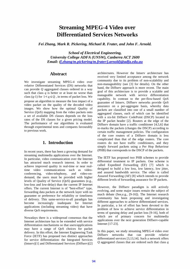
Streaming MPEG-4 Video over Differentiated Services Networks

Fei Zhang, Mark R. Pickering, Michael R. Frater, and John F. Arnold.

School of Electrical Engineering,

University College ADFA (UNSW), Canberra ACT 2600 Email: (f.zhang/m.pickering/m.frater/j.arnold)@adfa.edu.au

Abstract We investigate streaming MPEG-4 video over relative Differentiated Services (DS) networks that can provide Q aggregated classes ordered in a way such that class q is better or at least no worse than class (q-1) for 1 q Q< ≤ , in terms of packet loss. We propose an algorithm to measure the loss impact of a video packet on the quality of the decoded video images. We show how the optimal Quality of Service (QoS) mapping from the video packets onto a set of available DS classes depends on the loss rates of the DS classes for a given pricing model. The performance of our algorithms is evaluated through experimental tests and compares favourably to previous work.

1. Introduction In recent years, there has been a growing demand for streaming multimedia applications over the Internet. In particular, video communication over the Internet has attracted much research interest. In order to achieve improved quality in real-time or near real-time video communications such as video-conferencing, video-telephony, and video-on-demand, the users must be provided with higher levels of Quality of Service (QoS) guarantees (e.g., low-loss and low-delay) than the current IP Internet offers. The current Internet is of “best-effort” type, forwarding data packets at the network layer with no guarantee or preference for reliability or timeliness of delivery. This same-service-to-all paradigm has become increasingly inadequate for Internet applications (including streaming video) that have diverse QoS requirements. Nowadays there is a widespread consensus that the Internet architecture has to be extended with service differentiation mechanisms so that users/applications may have a range of QoS choices for packet delivery. In this effort, the Internet Engineering Task Force (IETF) has proposed two distinct approaches for service differentiation: the Integrated Services (Intserv)[1] and Differentiated Services (Diffserv)[2]

architectures. However the Intserv architecture has received very limited acceptance among the network community due to its problem of non-scalability and non-manageability (see [3] for details). On the other hand, the Diffserv approach is more recent. The main goal of this architecture is to provide a scalable and manageable network with service differentiation capability. In contrast to the per-flow-based QoS guarantee of Intserv, Diffserv networks provide QoS assurance on a per-aggregate basis, whereby data packets are classified into one of a small number of aggregated classes, each of which can be identified with a six-bit Diffserv CodePoint (DSCP) located in the IP packet header [2]. Routers at the edge of the Diffserv domain have a traffic conditioner [4,5,6] that re-marks the packets (changes the DSCP) according to certain traffic management policies. The configuration of the core routers of a Diffserv domain is less complicated than that of the edge routers. The core routers do not have traffic conditioners, and they simply forward packets using a Per Hop Behaviour (PHB) that corresponds to the DSCP of the packets. The IETF has proposed two PHB schemes to provide differential treatment to IP packets. One scheme is called Expedited Forwarding (EF) [7] which is designed to build a low loss, low latency, low jitter, and assured bandwidth service. The other is called Assured Forwarding (AF) [8] which intends to provide different levels of forwarding assurance for IP packets. However, the Diffserv paradigm is still actively evolving, and some major issues remain the subject of much debate (See,e.g., [9-16]). The Internet research community has been proposing and investigating different approaches to achieve differentiated services. In particular, a lot of effort has been devoted to the problem of how to achieve service differentiation in terms of queuing delay and packet loss [9-16], both of which are of primary concern for multimedia applications over the next generation Diffserv-capable Internet [17-23]. In this paper, we study streaming MPEG-4 video over Diffserv networks that can provide relative differentiated services [3,13,14]. Such a network offers Q aggregated classes that are ordered such that class q

is better or at least no worse than class (q-1) for 1 q Q< ≤ , in terms of local (per-hop) metrics for the queuing delay and/or packet dropping. We first examine the impact of a lost video packet on the quality of the decoded video images. Then we investigate the optimal mapping from the data packets onto the Diffserv classes to achieve maximal video quality subject to a given price constraint. We show how the optimal mapping depends on the loss rates and unit prices of the DS classes. We demonstrate that the new algorithms perform better than those proposed in Refs [17,18,19].

2. Packet Loss Impact on Video Quality

The MPEG-4 video coding standard specifies that the encoder have an error-resilient mode that enables it to compress a video sequence into a stream of video packets with approximately the same pre-set size. These video packets are coded independently and separated by a byte-aligned synchronisation marker, so that the decoder can correctly decode received packets even if some previous packets are lost or corrupted. We observe that the loss of some packets would result in greater quality degradation than the loss of some others because the quality will depend on how well the error can be concealed in the decoder. For example, if a video packet contains many scene change-induced Intra macroblocks, it would be difficult to conceal the loss of such a packet with either temporal or spatial concealment method. Another very important type of packet includes those with a Video Object Plane (VOP) header, which contains information such as coding type (I, P, or B-frame) and time stamp. The loss of a VOP header would result in an entire VOP being un-decodable. In order to use a Diffserv network effectively, it is important to know the loss impact of every packet, so that those packets with higher loss impact may be sent via an appropriate higher priority traffic class that suffers lower loss probability. (Here we only consider the loss effect. We assume delay and jitter effects can be absorbed by using a large play buffer in the decoder). To measure the loss impact of a video packet quantitatively, we assume that the decoder is using a normative error concealment algorithm: For the first I-frame we use the usual interpolation method to perform error concealment. For all subsequent frames we employ a temporal concealment scheme by using a neighbouring MB’s motion vectors, if available, or zero motion vector if no neighbour macroblock (MB) is available. Under such an error concealment scheme, if a packet is lost in the k-th frame, then the initial error will be

∑=i

ik fD 2||δ , (2.1)

where the sum is over all the errored pixels, and ifδ is the difference between the decoded signals with and without the error due to the packet loss. Such an initial error will propagate into the next frame (k+1) when the errored pixels are referenced

∑=+i

ik finD 21 ||)( δ (2.2)

where n(i) is the number of times the pixel i is referenced by the (k+1)-th frame. This temporal error propagation may only be stopped by Intra-refresh or I-frames. We consider an MPEG-4 compressed video sequence with periodic I-frames (I-frames can provide error-refresh, and they can be used to create trick modes such as fast-forward and fast rewind in applications like video-on-demand). If we assume that

≈+1kD kD , then the total squared error distortion due to the packet loss in the frame, which is k frames away from the immediately previous I-frame, would be

kI DkND )( −≈ , where IN is the period of the I-frame (i.e., an I-frame appears regularly once every

IN frames). Therefore, we define the loss impact of a

given packet in the k-th frame as ( )I kN k D− . This loss impact correctly reflects the fact that a packet loss in an I-frame will generally result in a greater impact on the video quality because the errors have a longer effect.

The present method is simpler than that proposed by Shin et al [17], where three factors were taken into account in determining the relative priority index of a video packet. The three factors are the initial error, the average motion vector size and the number of Intra macroblocks contained in a packet, with weights of 0.7,0.15, and 0.15 respectively. In section 4 we will compare the performance of these two methods.

3. Optimal QoS Mapping We consider N consecutive video packets, each of which has a loss impact denoted as iD . We assume that there is a set of available DS classes ,1q q Q≤ ≤ , each of which experiences an average

loss rate ql and attracts a unit price qP . Without loss of generality, we assume that the DS classes are ordered such that the loss rate is decreasing and the unit price increasing: 1 2 Ql l l> > > and

1 2 QP < P < < P .

To send a video packet stream over the Diffserv network, we must first assign each packet i with an appropriate DS class ( )q i . Similar to Ref. [17] we call such a mapping (from the packet to the DS classes) QoS mapping. The problem is to find an optimal QoS mapping that satisfies the given price

constraint, ( )1

N

q ii

P P=

≤∑ , where P is the budget for

the N packets, and minimize the loss impact

expressed as ( )1

N

i q ii

D l=∑ . Such an optimal QoS

mapping would also maximize the receiving video quality. To solve this optimisation problem, we first sort the N packets into ascending order according to the loss impact. Then it can be shown that the optimal mapping must be an ordered mapping such that the first 1K packets are mapped to the lowest priority DS class, the next 2 1K K− packets to the second lowest level DS class, and so on. Therefore, the total loss impact can be expressed as

(3.1) And the price constraint becomes

1 2 1

1 1 2 1 2 1

( , , , )( ) ( ) ,

Q

Q Q

K K KK P K K P N K P Pπ −

−

=

+ − + + − ≤

(3.2) This is an optimisation problem with (Q-1) integer decision variables 1 2 11 , QK K K N−≤ ≤ ≤ ≤ . The feasible solution region is defined by the price constraint (3.2) and the bandwidth constraints of each DS level based on traffic conditioning agreement. If only two DS classes are available, the optimisation problem can be solved analytically.

21

2 1

NP PKP P

−≈−

(3.3)

This equation clearly indicates that when the user is paying the base price 1P NP= , then 1K N= , meaning that all packets have to be sent via the low DS class (best-effort class). When P is increased the number of low priority packets 1K will be decreased, and the number of high priority packets will be

increased. In the extreme case where the user can pay the top price 2P NP= , then 1 0,K = which means that all the packets could be sent via the high priority class provided there was no bandwidth limit in the high class. When there are more than two DS levels to choose from, the optimal solution can be analysed with the method of Lagrange Multipliers. We consider the Lagrangian function,

1 2 1

1 2 1

( , , , )[ ( , , , ) ]

Q

Q

L J K K KK K K Pλ π

−

−

= −

−

(3.4)

Let the first-order derivatives of this function with respect to the variables qK and λ be zero, we obtain the following equation set:

1 1

1 2 1

( ) ( ) 0,

( , , , ) 0.qq q K q q

Q

l l D P P

K K K P

λ

π+ +

−

− − − =

− =

(3.5)

Eliminating the parameter λ we obtain the following recursive relation.

1

1 1

1 1

(P P )( )(P P )( )q q

q q q qK K

q q q q

l lD D

l l −

+ −

− +

− −=

− −, (3.6)

where q=2,3,….Q-1. This equation defines the relationship between the variables qK and 1qK − . In particular, a guidance analytical solution can be obtained if KD could be expressed as a simple

function of K, say KD K= . In general, however, we have to use a numerical algorithm to find the optimal solution We note that our algorithm solves the optimisation problem directly. This is in contrast to the simplified method used in [17,18,19], where the packets are classified into a number of categories, each was assigned with an average relative priority index (loss impact), and the optimal mapping from the categories to DS classes was searched for. Our optimisation algorithm can be ideally applied to segments of a relatively small number of data packets, which represent a video bit stream of a short duration, say a few seconds. Here the requirement of “small number of packets” is based on the consideration that sorting may be done quickly enough (near real-time). If the sorting and optimisation is done off-line, our algorithm can also be applied to a large number of packets. According to the works of Dovrolis et al [3,13,14], for relative differentiated networks the normalised loss

1 2

1 1

1 2 1

1 21 1 1

( , , , )

Q

Q

K K N

k k Q kk k K k K

J K K K

l D l D l D−

−

= = + = +

=

+ + +∑ ∑ ∑

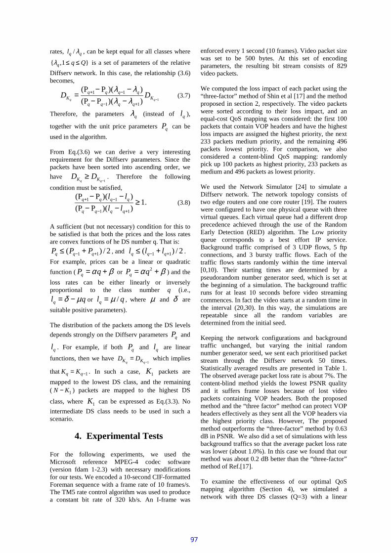
rates, /q ql λ , can be kept equal for all classes where

,1 q q Qλ ≤ ≤ is a set of parameters of the relative Diffserv network. In this case, the relationship (3.6) becomes,

1

1 1

1 1

(P P )( )(P P )( )q q

q q q qK K

q q q q

D Dλ λλ λ −

+ −

− +

− −=

− − (3.7)

Therefore, the parameters qλ (instead of ql ),

together with the unit price parameters qP can be used in the algorithm. From Eq.(3.6) we can derive a very interesting requirement for the Diffserv parameters. Since the packets have been sorted into ascending order, we have

1q qK KD D−

≥ . Therefore the following

condition must be satisfied,

1 1

1 1

(P P )( )1.

(P P )( )q q q q

q q q q

l ll l

+ −

− +

− −≥

− − (3.8)

A sufficient (but not necessary) condition for this to be satisfied is that both the prices and the loss rates are convex functions of he DS number q. That is:

1 1( ) / 2q q qP P P− +≤ + , and 1 1( ) / 2q q ql l l− +≤ + . For example, prices can be a linear or quadratic function ( qP qα β= + or 2

qP qα β= + ) and the loss rates can be either linearly or inversely proportional to the class number q (i.e.,

ql qδ µ= − or /ql qµ= , where µ and δ are suitable positive parameters). The distribution of the packets among the DS levels depends strongly on the Diffserv parameters qP and

ql . For example, if both qP and ql are linear

functions, then we have 1q qK KD D

−= which implies

that 1q qK K −= . In such a case, 1K packets are mapped to the lowest DS class, and the remaining ( 1N K− ) packets are mapped to the highest DS

class, where 1K can be expressed as Eq.(3.3). No intermediate DS class needs to be used in such a scenario.

4. Experimental Tests For the following experiments, we used the Microsoft reference MPEG-4 codec software (version fdam 1-2.3) with necessary modifications for our tests. We encoded a 10-second CIF-formatted Foreman sequence with a frame rate of 10 frames/s. The TM5 rate control algorithm was used to produce a constant bit rate of 320 kb/s. An I-frame was

enforced every 1 second (10 frames). Video packet size was set to be 500 bytes. At this set of encoding parameters, the resulting bit stream consists of 829 video packets. We computed the loss impact of each packet using the “three-factor” method of Shin et al [17] and the method proposed in section 2, respectively. The video packets were sorted according to their loss impact, and an equal-cost QoS mapping was considered: the first 100 packets that contain VOP headers and have the highest loss impacts are assigned the highest priority, the next 233 packets medium priority, and the remaining 496 packets lowest priority. For comparison, we also considered a content-blind QoS mapping: randomly pick up 100 packets as highest priority, 233 packets as medium and 496 packets as lowest priority. We used the Network Simulator [24] to simulate a Diffserv network. The network topology consists of two edge routers and one core router [19]. The routers were configured to have one physical queue with three virtual queues. Each virtual queue had a different drop precedence achieved through the use of the Random Early Detection (RED) algorithm. The Low priority queue corresponds to a best effort IP service. Background traffic comprised of 3 UDP flows, 5 ftp connections, and 3 bursty traffic flows. Each of the traffic flows starts randomly within the time interval [0,10). Their starting times are determined by a pseudorandom number generator seed, which is set at the beginning of a simulation. The background traffic runs for at least 10 seconds before video streaming commences. In fact the video starts at a random time in the interval (20,30). In this way, the simulations are repeatable since all the random variables are determined from the initial seed. Keeping the network configurations and background traffic unchanged, but varying the initial random number generator seed, we sent each prioritised packet stream through the Diffserv network 50 times. Statistically averaged results are presented in Table 1. The observed average packet loss rate is about 7%. The content-blind method yields the lowest PSNR quality and it suffers frame losses because of lost video packets containing VOP headers. Both the proposed method and the “three factor” method can protect VOP headers effectively as they sent all the VOP headers via the highest priority class. However, The proposed method outperforms the “three-factor” method by 0.63 dB in PSNR. We also did a set of simulations with less background traffics so that the average packet loss rate was lower (about 1.0%). In this case we found that our method was about 0.2 dB better than the “three-factor” method of Ref.[17].

To examine the effectiveness of our optimal QoS mapping algorithm (Section 4), we simulated a network with three DS classes (Q=3) with a linear

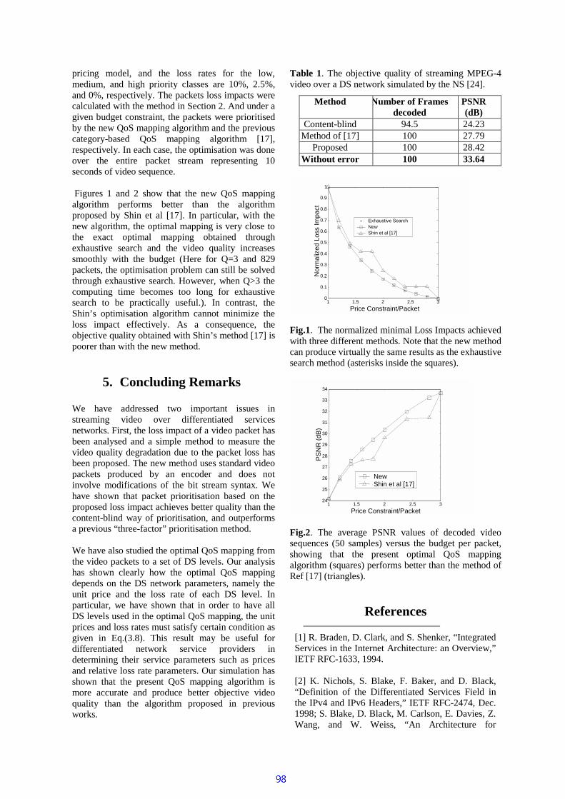
pricing model, and the loss rates for the low, medium, and high priority classes are 10%, 2.5%, and 0%, respectively. The packets loss impacts were calculated with the method in Section 2. And under a given budget constraint, the packets were prioritised by the new QoS mapping algorithm and the previous category-based QoS mapping algorithm [17], respectively. In each case, the optimisation was done over the entire packet stream representing 10 seconds of video sequence. Figures 1 and 2 show that the new QoS mapping algorithm performs better than the algorithm proposed by Shin et al [17]. In particular, with the new algorithm, the optimal mapping is very close to the exact optimal mapping obtained through exhaustive search and the video quality increases smoothly with the budget (Here for Q=3 and 829 packets, the optimisation problem can still be solved through exhaustive search. However, when Q>3 the computing time becomes too long for exhaustive search to be practically useful.). In contrast, the Shin’s optimisation algorithm cannot minimize the loss impact effectively. As a consequence, the objective quality obtained with Shin’s method [17] is poorer than with the new method.

5. Concluding Remarks We have addressed two important issues in streaming video over differentiated services networks. First, the loss impact of a video packet has been analysed and a simple method to measure the video quality degradation due to the packet loss has been proposed. The new method uses standard video packets produced by an encoder and does not involve modifications of the bit stream syntax. We have shown that packet prioritisation based on the proposed loss impact achieves better quality than the content-blind way of prioritisation, and outperforms a previous “three-factor” prioritisation method. We have also studied the optimal QoS mapping from the video packets to a set of DS levels. Our analysis has shown clearly how the optimal QoS mapping depends on the DS network parameters, namely the unit price and the loss rate of each DS level. In particular, we have shown that in order to have all DS levels used in the optimal QoS mapping, the unit prices and loss rates must satisfy certain condition as given in Eq.(3.8). This result may be useful for differentiated network service providers in determining their service parameters such as prices and relative loss rate parameters. Our simulation has shown that the present QoS mapping algorithm is more accurate and produce better objective video quality than the algorithm proposed in previous works.

Table 1. The objective quality of streaming MPEG-4 video over a DS network simulated by the NS [24].

1 1.5 2 2.5 3 0

0.1

0.2

0.3

0.4

0.5

0.6

0.7

0.8

0.9

1

Price Constraint/Packet N

orm

aliz

ed L

oss

Impa

ct

Exhaustive Search NewShin et al [17]

Fig.1. The normalized minimal Loss Impacts achieved with three different methods. Note that the new method can produce virtually the same results as the exhaustive search method (asterisks inside the squares).

1 1.5 2 2.5 3 24

25

26

27

28

29

30

31

32

33

34

Price Constraint/Packet

PSN

R (d

B)

NewShin et al [17]

Fig.2. The average PSNR values of decoded video sequences (50 samples) versus the budget per packet, showing that the present optimal QoS mapping algorithm (squares) performs better than the method of Ref [17] (triangles).

References

[1] R. Braden, D. Clark, and S. Shenker, “Integrated Services in the Internet Architecture: an Overview,” IETF RFC-1633, 1994. [2] K. Nichols, S. Blake, F. Baker, and D. Black, “Definition of the Differentiated Services Field in the IPv4 and IPv6 Headers,” IETF RFC-2474, Dec. 1998; S. Blake, D. Black, M. Carlson, E. Davies, Z. Wang, and W. Weiss, “An Architecture for

Method Number of Frames decoded

PSNR (dB)

Content-blind 94.5 24.23 Method of [17] 100 27.79

Proposed 100 28.42 Without error 100 33.64

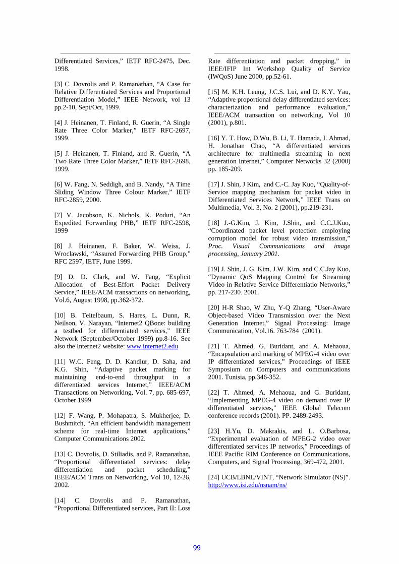
Differentiated Services,” IETF RFC-2475, Dec. 1998. [3] C. Dovrolis and P. Ramanathan, “A Case for Relative Differentiated Services and Proportional Differentiation Model,” IEEE Network, vol 13 pp.2-10, Sept/Oct, 1999. [4] J. Heinanen, T. Finland, R. Guerin, “A Single Rate Three Color Marker,” IETF RFC-2697, 1999. [5] J. Heinanen, T. Finland, and R. Guerin, “A Two Rate Three Color Marker,” IETF RFC-2698, 1999. [6] W. Fang, N. Seddigh, and B. Nandy, “A Time Sliding Window Three Colour Marker,” IETF RFC-2859, 2000. [7] V. Jacobson, K. Nichols, K. Poduri, “An Expedited Forwarding PHB,” IETF RFC-2598, 1999 [8] J. Heinanen, F. Baker, W. Weiss, J. Wroclawski, “Assured Forwarding PHB Group,” RFC 2597, IETF, June 1999. [9] D. D. Clark, and W. Fang, “Explicit Allocation of Best-Effort Packet Delivery Service,” IEEE/ACM transactions on networking, Vol.6, August 1998, pp.362-372. [10] B. Teitelbaum, S. Hares, L. Dunn, R. Neilson, V. Narayan, “Internet2 QBone: building a testbed for differentiated services,” IEEE Network (September/October 1999) pp.8-16. See also the Internet2 website: www.internet2.edu [11] W.C. Feng, D. D. Kandlur, D. Saha, and K.G. Shin, “Adaptive packet marking for maintaining end-to-end throughput in a differentiated services Internet,” IEEE/ACM Transactions on Networking, Vol. 7, pp. 685-697, October 1999 [12] F. Wang, P. Mohapatra, S. Mukherjee, D. Bushmitch, “An efficient bandwidth management scheme for real-time Internet applications,” Computer Communications 2002. [13] C. Dovrolis, D. Stiliadis, and P. Ramanathan, “Proportional differentiated services: delay differentiation and packet scheduling,” IEEE/ACM Trans on Networking, Vol 10, 12-26, 2002. [14] C. Dovrolis and P. Ramanathan, “Proportional Differentiated services, Part II: Loss

Rate differentiation and packet dropping,” in IEEE/IFIP Int Workshop Quality of Service (IWQoS) June 2000, pp.52-61. [15] M. K.H. Leung, J.C.S. Lui, and D. K.Y. Yau, “Adaptive proportional delay differentiated services: characterization and performance evaluation,” IEEE/ACM transaction on networking, Vol 10 (2001), p.801. [16] Y. T. How, D.Wu, B. Li, T. Hamada, I. Ahmad, H. Jonathan Chao, “A differentiated services architecture for multimedia streaming in next generation Internet,” Computer Networks 32 (2000) pp. 185-209. [17] J. Shin, J Kim, and C.-C. Jay Kuo, “Quality-of-Service mapping mechanism for packet video in Differentiated Services Network,” IEEE Trans on Multimedia, Vol. 3, No. 2 (2001), pp.219-231. [18] J.-G.Kim, J. Kim, J.Shin, and C.C.J.Kuo, “Coordinated packet level protection employing corruption model for robust video transmission,” Proc. Visual Communications and image processing, January 2001. [19] J. Shin, J. G. Kim, J.W. Kim, and C.C.Jay Kuo, “Dynamic QoS Mapping Control for Streaming Video in Relative Service Differentiatio Networks,” pp. 217-230. 2001. [20] H-R Shao, W Zhu, Y-Q Zhang, “User-Aware Object-based Video Transmission over the Next Generation Internet,” Signal Processing: Image Communication, Vol.16. 763-784 (2001). [21] T. Ahmed, G. Buridant, and A. Mehaoua, “Encapsulation and marking of MPEG-4 video over IP differentiated services,” Proceedings of IEEE Symposium on Computers and communications 2001. Tunisia, pp.346-352. [22] T. Ahmed, A. Mehaoua, and G. Buridant, “Implementing MPEG-4 video on demand over IP differentiated services,” IEEE Global Telecom conference records (2001). PP. 2489-2493. [23] H.Yu, D. Makrakis, and L. O.Barbosa, “Experimental evaluation of MPEG-2 video over differentiated services IP networks,” Proceedings of IEEE Pacific RIM Conference on Communications, Computers, and Signal Processing, 369-472, 2001. [24] UCB/LBNL/VINT, “Network Simulator (NS)”. http://www.isi.edu/nsnam/ns/

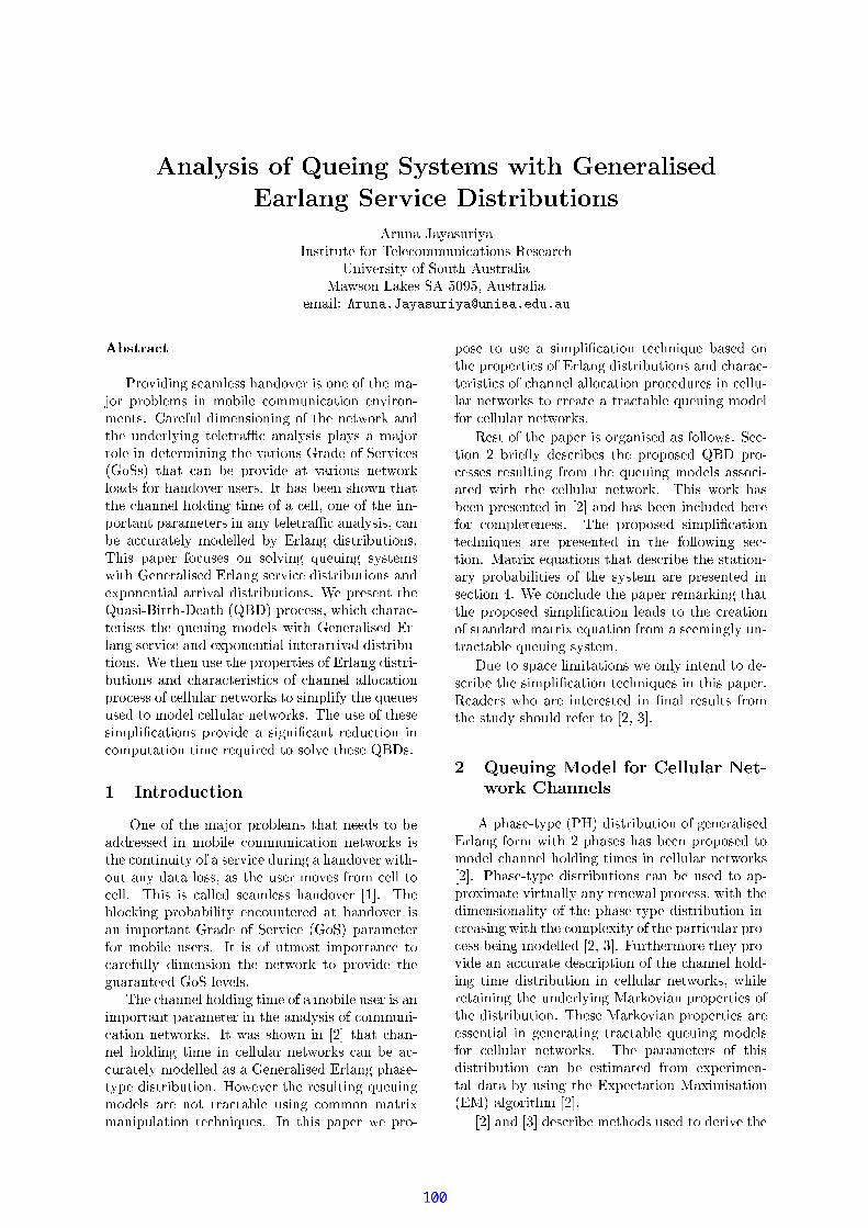
! "$#&%'$ ()* '+,-.'/ 01324 $'+ 567$,86

9;:=<?>A@CB,@ED,@FG<?:=H D,@I >AFKJ=H J=<LJ=MNPO:;QRMTS MVUWOXYXZ<?>?H[UT@\J=H O>AF^]^MVFGMV@_:`U`a

b >?H cMT:`FGH JKD1O_Ned O<LJ=a9;<AFKJ=:`@_S H[@f @Eg;FGO>ihR@_jMVF;dL9lk_mn,kLo 9;<AFKJ=:`@_S H[@

MTXC@_H Sqper s,t uAvxw=y,vz?v?EtLs|EzLv ~_t,u|vewG,_twKv_t

1TT\?_ :=O\c H[LH >?+FGMV@_XYS MVF=FxaA@_>ALO\cMT:H[FO>?M;O_NJ=a?MXC@\

O:?:=O?S MTXCFH >XYO?H S MUWOXYXZ<?>?H[UT@\J=H O>.MT> c H :=O>LXYMT>,J`FTZ@_:=MWNP<?SLH XYMT>AFGH O>?H >?iO_NeJ=a?M>?MWJKgO:=j@_>AJ=a?Mi<?>ALMT:=S D H >?J=MTS MWJ=:`@\1U@_>A@_S DLFGH[F+?S[@EDLF@XC@ O::=OS MH >LMWJ=MT:=XYH >?H >?YJ=a?M+c\@_:=H O<AF^(:`@LM$O_Nxd MT:=c H[UWMVF (O dLF`CJ=aA@\JUT@_> M?:=O\c H[LM@\J¡c\@_:=H O<AF1>?MWJKgO:=jS O,@?FNPO:;aA@_>ALO\cMT:<AFGMT:`FT I J;aA@F^ MTMT>¢FGa?O\g^>J=aA@\JJ=a?MZU`aA@_>?>?MTSa?OS[LH >?YJ=H XYM+O_Nx@CUWMTS SqoAO>?M$O_NJ=a?M+H X O:GJ`@_>,JeA@_:`@_XYMWJ=MT:`F£H >C@_> DJ=MTS MWJ=:`@\1U^@_>A@_S DLFGH[FTo_UT@_> M@UTUW<?:`@\J=MTS DXYOLLMTS S MV¤ D¤¥x:=S[@_>?¦LH[FKJ=:=H ?<LJ=H O>AFTQa?H[FA@_ MT:¡NPOLUW<AFGMVFO>6FGOS c H >?§,<?MT<?H >?FGDLFKJ=MTXCFg^H J=a¡(MT>?MT:`@_S H[FGMVC¥x:=S[@_>?+FGMT:=c H[UWMLH[FKJ=:=H ?<LJ=H O>AF@_>AMW¨L O>?MT>,J=H[@_S£@_:=:=H c\@_SRLH[FKJ=:=H ?<LJ=H O>AFT^©M+?:=MVFGMT>,J;J=a?Mª <A@FGH ¬«H :GJ=aL¬­MV@\J=a ª «­x?:=OLUWMVF=FTog^a?H[U`aU`aA@_:`@U®J=MT:=H[FGMVF$J=a?M§,<?MT<?H >?¢XYOLLMTS[FZg^H J=a8(MT>?MT:`@_S H[FGMV¦¥x:GS[@_>?ZFGMT:=c H[UWM@_>ACMW¨L O>?MT>,J=H[@_S H >,J=MT:`@_:=:=H c\@_SALH[FKJ=:=H ?<LJ=H O>AFT£©MJ=a?MT><AFGMJ=a?M?:=O MT:GJ=H MVF£O_N¥x:=S[@_>?(LH[FKJ=:=H ?<LJ=H O>AFZ@_>AU`aA@_:`@U®J=MT:=H[FKJ=H[UTFO_N;U`aA@_>?>?MTS@_S S OLUT@\J=H O>?:=OLUWMVF=F£O_N UWMTS S <?S[@_:>?MWJKgO:=jLFJ=O$FGH XY?S H NPD$J=a?M^§,<?MT<?MVF<AFGMVYJ=OZXYOLLMTSUWMTS S <?S[@_:>?MWJKgO:=jLFT£Qa?M<AFGMO_NJ=a?MVFGMFGH XY?S H ¯ UT@\J=H O>AFZ?:=O\c H[LMi@FGH >?H ¯ UT@_>,J:=MVL<AU®J=H O>H >UWOXY?<LJ`@\J=H O>J=H XYM$:=MV§,<?H :=MV1J=O1FGOS cMJ=a?MVFGM ª «­(FT

° ±,²³L´?µ^¶·¸ ³?¹Kµ²º >?MYO_NJ=a?MYXC@ O:$?:=O?S MTXCF(J=aA@\J$>?MTMV?FJ=O¡ M

@?L:=MVF=FGMV¤H >.XYO?H S M¢UWOXYXZ<?>?H[UT@\J=H O>.>?MWJKgO:=jLFYH[FJ=a?MUWO>,J=H > <?H JKD(O_N?@;FGMT:=c H[UWML<?:=H >?@^aA@_>ALO\cMT:g^H J=aLO<LJ@_> D¡?@\J`@CS O,F=FTo@F^J=a?M<AFGMT:XYO\cMVFNP:=OX»UWMTS SRJ=OUWMTS SqQa?H[FCH[F1UT@_S S MV¤FGMV@_XYS MVF=FYaA@_>ALO\cMT:¼ ½®¾¿Qa?M?S OLU`j H >??:=OA@_?H S H JKD¦MT>AUWO<?>,J=MT:=MV¤@\J1aA@_>ALO\cMT:YH[F@_>H XY O:GJ`@_>,J(:`@LMYO_N;d MT:=c H[UWM (O d?A@_:`@_XYMWJ=MT:NPO:YXYO?H S Mi<AFGMT:`FT I JYH[FYO_N<LJ=XYO,FKJCH XY O:GJ`@_>AUWMJ=OUT@_:=MWNP<?S S DLH XYMT>AFGH O>J=a?M>?MWJKgO:=j¤J=O¤?:=O\c H[LM¢J=a?M<A@_:`@_>,J=MTMVi(O d1S MTcMTS[FTQa?MU`aA@_>?>?MTSa?OS[LH >?;J=H XYMO_NA@^XYO?H S M<AFGMT:RH[F£@_>

H XY O:GJ`@_>,JA@_:`@_XYMWJ=MT:H >1J=a?M$@_>A@_S DLFGH[FxO_N£UWOXYXZ<?>?H UT@\J=H O>>?MWJKgO:=jLFT I JZg@F+FGa?O\g^>H >¼ ÀE¾J=aA@\JU`aA@_>L>?MTSa?OS[LH >?J=H XYMiH >8UWMTS S <?S[@_:Z>?MWJKgO:=jLF+UT@_>¦ Mi@U®UW<?:`@\J=MTS DYXYOLLMTS S MV@F@(MT>?MT:`@_S H[FGMV1¥x:=S[@_>?+?aA@FGMWJKD MZLH[FKJ=:=H ?<LJ=H O>^Á;O\gMTcMT:J=a?MZ:=MVFG<?S J=H >?1§,<?MT<?H >?XYOLLMTS[Fi@_:=M¢>?O_JJ=:`@U®J`@_?S M<AFGH >?8UWOXYXYO>XC@\J=:=H ¨XC@_>?H ?<?S[@\J=H O>J=MVU`a?>?H[§,<?MVFT I >8J=a?H[FA@_ MT:YgMi?:=O_

O,FGM¡J=O<AFGM¢@FGH XY?S H ¯ UT@\J=H O>¤J=MVU`a?>?H[§,<?M¢A@FGMV¤O>J=a?M;?:=O MT:GJ=H MVFxO_N¥x:=S[@_>?$LH[FKJ=:=H ?<LJ=H O>AF@_>ACU`aA@_:`@U®J=MT:=H[FKJ=H[UTFO_N£U`aA@_>?>?MTS @_S S OLUT@\J=H O>1?:=OLUWMVL<?:=MVFxH >iUWMTS S <LS[@_:>?MWJKgO:=jLFJ=OUW:=MV@\J=M+@CJ=:`@U®J`@_?S M+§,<?MT<?H >?1XYOLLMTSNPO:;UWMTS S <?S[@_:^>?MWJKgO:=jLFT]^MVFKJ^O_NRJ=a?M$A@_ MT:^H[FO:=,@_>?H[FGMV1@FNPOS S O\g;FTxd MVU®

J=H O>À?:=H MWÂAD¤LMVF=UW:=H MVFYJ=a?M?:=O O,FGMV ª «­»?:=O_UWMVF=FGMVF$:=MVFG<?S J=H >?¡NP:=OXÃJ=a?M§,<?MT<?H >?¢XYOLLMTS[F+@F=FGOLUWH @\J=MV.g^H J=aJ=a?MUWMTS S <?S[@_:>?MWJKgO:=jÄQa?H[FgO:=j¤aA@F MTMT>¢?:=MVFGMT>,J=MViH >8¼ ÀV¾e@_>A¡aA@F; MTMT>H >AUWS <ALMVa?MT:=MNPO:¦UWOXY?S MWJ=MT>?MVF=FT!Qa?M?:=O O,FGMVÅFGH XY?S H ¯ UT@\J=H O>J=MVU`a?>?H[§,<?MVF@_:=M?:=MVFGMT>,J=MVÆH >ÆJ=a?M7NPOS S O\g^H >?ÄFGMVU®J=H O> f @\J=:=H ¨iMV§,<A@\J=H O>AFJ=aA@\J(LMVF=UW:=H M$J=a?MZFKJ`@\J=H O>L@_:=D?:=OA@_?H S H J=H MVFO_N(J=a?M¢FGDLFKJ=MTXÇ@_:=Mi?:=MVFGMT>,J=MV8H >FGMVU®J=H O>iÈA©M+UWO>AUWS <ALM(J=a?MA@_ MT:^:=MTXC@_:=j H >?+J=aA@\JJ=a?MC?:=O O,FGMVFGH XY?S H ¯ UT@\J=H O>S MV@?F(J=O¡J=a?M1UW:=MV@\J=H O>O_NFKJ`@_>A?@_:`ZXC@\J=:=H ¨ZMV§,<A@\J=H O>ZNP:=OXÄ@FGMTMTXYH >?S DZ<?>LJ=:`@U®J`@_?S M$§,<?MT<?H >?CFGDLFKJ=MTX¡­<?MJ=OFGA@UWM;S H XYH J`@\J=H O>AFgMO>?S DH >,J=MT>ACJ=OLMW

F=UW:=H M(J=a?M$FGH XY?S H ¯ UT@\J=H O>J=MVU`a?>?H[§,<?MVFH >J=a?H[FA@_ MT:V]^MV@LMT:`FZg^a?O@_:=MH >,J=MT:=MVFKJ=MV¦H >8¯A>A@_S:=MVFG<?S J`FZNP:=OXJ=a?M+FKJ=<ALDiFGa?O<?S[:=MWNPMT:J=O¢¼ À oAÉE¾¿

Ê Ë8·;ÌR·¹G²;ÍÆÎϵ^¶;ÌRÐYÑ`µx´ÒÌRÐGÐG·ÐKÓ´¤Ô̳,ÕÖ µx´?×ØÒÙ;Óe²²;ÌRÐGÚ9?aA@FGMWqJKD M Á(LH[FKJ=:=H ?<LJ=H O>1O_NMT>?MT:`@_S H[FGMV

¥x:=S[@_>?CNPO:=XØg^H J=a¦ÀC?aA@FGMVFaA@F MTMT>?:=O O,FGMV¡J=OXYOLLMTS£U`aA@_>?>?MTSRa?OS[LH >?YJ=H XYMVFH >¢UWMTS S <?S[@_:;>?MWJKgO:=jLF¼ ÀE¾¿ aA@FGMWqJKD MYLH[FKJ=:=H ?<LJ=H O>AF+UT@_> M1<AFGMVJ=O¢@_L?:=OE¨LH XC@\J=M^c H :GJ=<A@_S S D@_> DZ:=MT>?MTg@_SL?:=OLUWMVF=FTog^H J=aYJ=a?MLH XYMT>AFGH O>A@_S H JKD¢O_NJ=a?MC?aA@FGMWqJKD MCLH[FKJ=:=H ?<LJ=H O>H >LUW:=MV@FGH >?^g^H J=aJ=a?MUWOXY?S MW¨LH JKD(O_N J=a?MA@_:GJ=H[UW<?S[@_:?:=O_UWMVF=Fx MTH >?XYOLLMTS S MV¢¼ ÀLo ÉE¾¿eÛ?<?:GJ=a?MT:=XYO:=M^J=a?MTDC?:=O_c H[LMZ@_>¢@UTUW<?:`@\J=M$LMVF=UW:=H LJ=H O>¡O_NJ=a?MU`aA@_>?>?MTSa?OS[ H >?J=H XYMLH[FKJ=:=H ?<LJ=H O>8H >UWMTS S <?S[@_:Y>?MWJKgO:=jLFTog^a?H S M:=MWJ`@_H >?H >?YJ=a?M+<?>ALMT:=S D H >? f @_:=jO\c H[@_>?:=O MT:GJ=H MVF^O_NJ=a?M+LH[FKJ=:=H ?<LJ=H O>xQa?MVFGM f @_:=jO\c H[@_>1?:=O MT:GJ=H MVF^@_:=MMVF=FGMT>,J=H[@_SH >MT>?MT:`@\J=H >?¡J=:`@U®J`@_?S M§,<?MT<?H >?XYOLLMTS[FNPO:UWMTS S <?S[@_:>?MWJKgO:=jLFTÜQa?MA@_:`@_XYMWJ=MT:`FO_NJ=a?H[FLH[FKJ=:=H ?<LJ=H O>ÄUT@_>l M8MVFKJ=H XC@\J=MV6NP:=OX!MW¨L MT:=H XYMT>LJ`@_S?@\J`@¡ D<AFGH >?iJ=a?M¥e¨L MVU®J`@\J=H O> f @\¨LH XYH[F=@\J=H O> ¥ f @_S O:=H J=a?Xü ÀE¾¿¼ ÀE¾ @_>A¡¼ É\¾LMVF=UW:=H M^XYMWJ=a?OL?Fe<AFGMVJ=O+LMT:=H cMJ=a?M

U`aA@_>?>?MTSAa?OS[LH >?+J=H XYM(LH[FKJ=:=H ?<LJ=H O>CNPO:UWMTS S <?S[@_:>?MWJGgO:=jLFRJ=a?:=O<?a>?MWJKgO:=jZFGH XZ<?S[@\J=H O>XYOLLMTS[FT b FGM^O_N¥ f @_S O:=H J=a?X7J=O@_??:=OE¨LH XC@\J=MeJ=a?M^@U®J=<A@_SLLH[FKJ=:=H ?<LJ=H O>Cg^H J=a@$MT>?MT:`@_S H[FGMVY¥x:=S[@_>?+LH[FKJ=:=H ?<LJ=H O>Cg^H J=aiÀ?aA@FGMVFH[F?:=MVFGMT>,J=MV1H >¼ ÉE¾R@_>A¼ È_¾¿x9;:=:=H c\@_S[FO_NR>?MTg@_>A$aA@_>ALO\cMT:R<AFGMT:`F£@_:=MxXYOLLMTS S MV+g^H J=aZMW¨L O>?MT>,J=H[@_SLH[FKJ=:=H ?<LJ=H O>AFg^H J=a¢@_??:=O?:=H[@\J=MA@_:`@_XYMWJ=MT:`FT9F=FG<?XYH >?Z@_>YMW¨L O>?MT>,J=H[@_S?H >,J=MT:`@_:=:=H c\@_S?LH[FKJ=:=H ?<L

J=H O>@_>AZ@;?aA@FGMWqJKD MFGMT:=c H[UWMLH[FKJ=:=H ?<LJ=H O>o_@(UWMTS S <LS[@_:>?MWJKgO:=jCg^H J=aU`aA@_>?>?MTS[F MT:;UWMTS SUT@_>i M$XYOL MTS S MV@Fi@_>6§,<?MT<?M¤¼ kV¾¿ Qa?M:=MVFG<?S JGH >?§,<?MT<?H >?ZFGDLFKJ=MTX XC@ED>?O_J MJ=:`@U®J`@_?S M;MTcMT>YNPO:XYOLLMT:`@\J=Mc\@_S <?MVFRO_N e¥§,<A@\J=H O> ½ERFGa?O\g;FJ=a?M:`@\J=MJ=:`@_>AFGH J=H O>CXC@\J=:=H ¨CO: ª XC@\J=:=H ¨YNPO:@_>§,<?MT<?Moeg^a?H[U`a8XYOLLMTS[F@UWMTS Sg^H J=aU`aA@_>?>?MTS[FT I >MV§,<A@\J=H O> ½EeH JUT@_>1 MOAFGMT:=cMVZJ=aA@\J H[FxO_N?S OLU`jJ=:=H ¬LH[@_O>A@_S NPO:=X ¼ kV¾¿

! #"$%&"'( )"* % "$+ #", -... . . . . . . . . .... ... "* 0/"$1/2"%/. . . . . . . . .3"* 54 6879:"$%4 6879;"'4 6879 "* 06 "$16

< ==============>?0@BA9F=FG<?XYH >?;MW¨L O>?MT>,J=H[@_S@_:=:=H c\@_S\?:=OLUWMVF=Fg^H J=a$:`@\J=MC oVJ=a?MxXC@\J=:=H[UWMVF:DEGF'D$H@_>A!D*Ix@_:=MeLMW¯A>?MV$@Fx¼ k oEÀV¾¿o

DEKJ C L ÀD$HMJ C É,D*INJ F È ©.a?MT:=MPOH[FYJ=a?MH >?H J=H[@_S;?:=OA@_?H S H JKDcMVU®J=O:CO_N(J=a?M ÁÅFGMT:=c H[UWMLH[FKJ=:=H ?<LJ=H O>@_>A H[F(@UWOS <?XY>cMVU®J=O:A@_:GJ=H J=H O>O_NAJ=a?M:`@\J=MJ=:`@_>AFGH J=H O>ZXC@\J=:=H ¨$$Q&RO_NAJ=a?M ÁLH[FKJ=:=H ?<LJ=H O>o?H cMT>iH >¡MV§,<A@\J=H O> k®

$Q&RJTS*UVUXW2Y kQa?M^UWO>AFKJ=:=<AU®J=H O>ZO_NXC@\J=:=H[UWMVF EZ5F H,Z@_>A I'Z

NPO:@MT>?MT:`@_SZ?aA@FGMJKD MLH[FKJ=:=H ?<LJ=H O>lH[F:`@\J=a?MT:UWOXY?S MW¨Y@_>A:=MV§,<?H :=MVFS MT>?_J=a D@_>AZJ=MVLH O<AFxUWOXY?<LJ`@\J=H O>AFT£Á;O\gMTcMT:VoEgMaA@EcMH[LMT>,J=H ¯AMVZFGOXYM?:=O MT:GJ=H MVFO_N MT>?MT:`@_S H[FGMVZ¥x:=S[@_>?(LH[FKJ=:=H ?<LJ=H O>AFg^a?H[U`aYFGH X?S H NPDJ=a?MVFGMUT@_S[UW<?S[@\J=H O>AFCJ=O@:=MV@\JMW¨ J=MT>,JV Qa?M>?MW¨ J(FGMVU®J=H O>¡O_NJ=a?H[F^A@_ MT:(LMVF=UW:=H MVFJ=a?M+?:=O O,FGMVFGH XY?S H ¯ UT@\J=H O>AF@_>A1@_S O:=H J=a?XCFeS MV@LH >?$J=O+J=a?M(UWO>LFKJ=:=<AU®J=H O>8O_NJ=:`@U®J`@_?S M[ÏXC@\J=:=H ¨NPO:J=a?M§,<?MT<?H >??:=OLUWMVF=FTR©M@F=FG<?XYMJ=a?MFGMT:=c H[UWM^LH[FKJ=:=H ?<LJ=H O>YH cMT> DCMV§,<A@\J=H O> 1\ eJ=a?:=O<?a?O<LJJ=a?M:=MVFKJO_NJ=a?MA@_ MT:V

W J S^]`_ H _ Im ]`_ I Y 1\

]^O\gFG<?XCFNPO:@_> DY:`@\J=M;J=:`@_>AFGH J=H O>XC@\J=:=H ¨1@_:=MbaTMT:=O¼ kE¾¿oL:=MVFG<?S J=H >?YH >o

J S m_ I Y F 0c g^a?MT:=M W @_>A @_:=MJ=a?MA@_:GJ=H J=H O>CXC@\J=:=H[UWMVFeO_Nd$Q&R@F^LMVF=UW:=H MVFH >¡MV§,<A@\J=H O> k®

e fhg9ikjlgnmognmqpÌ´srÌ´(t¹¬³?ÙÓ2u.ÌR²ÕÌ´?ÓeÐG¹GÚ,ÌR¶wv¡´AÐKÓe²;ÍxpÌ´sr;¹G¸Ì(y¹GÚ³L´A¹,z(·Õ³?¹Kµ²I >"J=a?M ?:=MTc H O<AFÏFGMVU®J=H O>"gM FGMTS MVU®J=MVJ=a?M¤§,<?MT<?MYJ=OXYOLLMTS@UWMTS Sg^H J=a.U`aA@_>L

>?MTS[FT9ÃL:`@Eg^A@U`j¦H >.<AFGH >?¦J=a?M@_ O\cM¡XYOLLMTS;J=O:=MT?:=MVFGMT>,J(XYO?H S MY>?MWJKgO:=jUWMTS S[F(H[FJ=aA@\JJ=a?MCFGH aTMO_NJ=a?Mi:`@\J=M1J=:`@_>AFGH J=H O>¦XC@\J=:=H ¨LMT MT>A?FO>¦J=a?Mi> <?X MT:(O_NU`aA@_>?>?MTS[F(@Ec\@_H S[@_?S M+H >@UWMTS Sq9F;J=a?MYFGH aTMZO_NJ=a?Mi?S OLU`jXC@\J=:=H ¨¦@\JS MTcMTS|H[FZO>O:`LMT:~ ZIZ¼ \ ¾NPO:C@FGMT:=c H[UWMiLH[FKJ=:=H ?<LJ=H O>¤O_NÀ?aA@FGMVFToeJ=a?MkXC@\J=:=H ¨ MVUWOXYMVF^<?>?XC@_>A@_MV@_?S M(NPO:^>?MWJKgO:=jLFg^H J=aS[@_:=MC> <?XZ MT:ZO_N;U`aA@_>?>?MTS[FZ@Ec\@_H S[@_?S MC MT:UWMTS Sq¢Û?<LJ=<?:=MXYO?H S M>?MWJKgO:=jLF1H >,J=MT>AJ=O¤?:=O\c H[LM@8S[@_:=M> <?XZ MT:ZO_N^U`aA@_>?>?MTS[F+ MT:ZUWMTS SxJ=OFG<?? O:GJ$J=a?Ma?H a?@\J`@¡:`@\J=MFGMT:=c H[UWMVF(J=aA@\JZg^H S S M@Ec\@_H S[@_?S MiQa?MT:=MWNPO:=MJ=a?MCXYMWJ=a?OL?F+@Ec\@_H S[@_?S MYH >.¼ kV¾UT@_>?>?O_J$ M1<AFGMVJ=Oi¯A>AJ=a?MY?S OLU`j H >?¡?:=OA@_?H S H J=H MVF(MW¨L MT:=H MT>AUWMV D>?MTgÃ@_>AaA@_>ALO\cMT:1<AFGMT:`F1H >J=a?MXYO?H S M>?MWJKgO:=jMT> c H :=O>?XYMT>,JV9FGH XY?S H ¯ UT@\J=H O>iUT@_> MXC@LMJ=OZJ=a?M XC@\J=:=H ¨

D¦OAFGMT:=c H >?FGOXYMi?:=O MT:GJ=H MVFZO_N;J=a?M¥x:=S[@_>?LH[FKJ=:=H ?<LJ=H O>¦@_>A¢J=a?MC MTaA@Ec H O<?:O_NFGMT:=cMT:`F(@\J+XYO?H S MUWMTS S[FT I >FGMT:=cMT:`F1g^H J=a7¥x:=S[@_>?¤LH[FKJ=:=H ?<LJ=H O>AFTo;J=a?M<AFGMT:`FC@_S g@EDLFYFKJ`@_:GJYJ=a?M¢FGMT:=c H[UWM¡H >¤J=a?M¯A:`FKJC?aA@FGM@_>AXYO\cMYO>J=O¡J=a?MC>?MW¨ J+?aA@FGMCg^H J=a¦?:=OA@_?H S H JKD½O>AUWM1J=a?M¡FGO O<?:=>¦H >¦J=aA@\JY?aA@FGMH[FZO\cMT:V b FGMT:`Fg^a?O¯A>?H[FGa¤J=a?M¢FGO O<?:=>8H >¤J=a?MS[@FKJ1?aA@FGMLMTA@_:GJJ=a?M1FGDLFKJ=MTX¡Y©.a?MT>J=a?MT:=MC@_:=MÏ<AFGMT:`FH >J=a?M1FGDLFKJ=MTX H J¡H[FH :=:=MTS MTc\@_>,Jig^a?H[U`aO_N+J=a?MVFGMk!<AFGMT:`Fi@_:=M@\J^g^a?H[U`aiFGMT:=cMT:@_>AFGH XYH S[@_:=S DCg^a?OZ¯A>?H[FGa?MVF^FGMT:=c H[UWM¯A:`FKJVQa?H[FCS MV@?FC<AFJ=OUWOXZ?H >?M¢@_S SJ=a?M<AFGMT:`FYH >J=a?MF=@_XYM(FGMT:=c H[UWM?aA@FGMJ=O@FGH >?S M(FGMT:=cMT:g^H J=a1J=a?MFGMT:=c H[UWM;:`@\J=M;MV§,<?H c\@_S MT>,JJ=O+J=a?M(UWOXZ?H >?MVC:`@\J=M;O_NR@_S SJ=a?MFGMT:=cMT:`FT b FGH >?;J=a?H[FFGH XY?S H ¯ UT@\J=H O>Z@_>A+@FGMT:=c H[UWMLH[FKJ=:=H ?<LJ=H O>O_NJKgO¡?aA@FGMVFToJ=a?MC> <?XZ MT:+O_N^LH MT:GMT>,JZFKJ`@\J=MVF O,F=FGH ?S MYH >J=a?MCFGDLFKJ=MTX g^a?MT>J=a?MT:=M1@_:=MÃ<AFGMT:`FH >iJ=a?M+FGDLFKJ=MTX @_:=M(H cMT>iH >Q£@_?S MY½Qa?MVFGMFGH XY?S H ¯ UT@\J=H O>AF@_S S O\g;FJ=O:=MT?:=MVFGMT>,JCJ=a?M

FGDLFKJ=MTXÅg^H J=aC@:=MVL<AUWMVFKJ`@\J=M;FGA@UWMQa?M^>?MTgFKJ`@\J=MFGA@UWM$UT@_>i M+LMW¯A>?MV¡@FNPOS S O\g;FTp > <?XZ MT:^O_N<AFGMT:`FH[F?aA@FGMY½ HT®o?> <?XZ MT:^O_N

<AFGMT:`FH >¡?aA@FGM+À &IEbQa?H[F:=MVL<AUWMVF;J=a?MFGH aTMZO_NeJ=a?MZXC@\J=:=H ¨¢@\J(S MTcMTS J=O ½E®Qa?M+g^a?OS M+FGDLFKJ=MTX UT@_> MZ@_:=:`@_>?MV1H >,J=OJKgO_¬LH XYMT>AFGH O>A@_SUWO>,J=H > <?O<AFJ=H XYM f @_:=jO\c7U`aA@_H >g^H J=aiJ=a?MNPOS S O\g^H >?CFKJ`@\J=M$FGA@UWMp

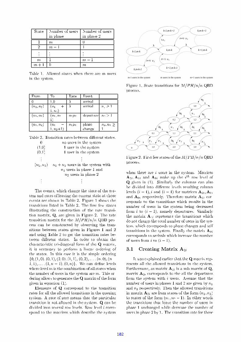
d,J`@\J=M ;<?XZ MT:O_N<AFGMT:`FH >¡?aA@FGM

;<?XZ MT:O_N<AFGMT:`FH >¡?aA@FGM+À

½ mÀ ] ½ ½ ½ ] ½(.½ m

Q£@_?S M½19;S S O\gMVFKJ`@\J=MVFg^a?MT>J=a?MT:=M1@_:=MÏ<AFGMT:`FH >iJ=a?M+FGDLFKJ=MTX¡

@ ? ! A ? #"@ A %$ @? ! A ? ! &@BA (' )*+ , - @? ! A ? .&@ " @BA '& *0/+1

2 /+03 4$@

Q£@_?S M;ÀL£QR:`@_>AFGH J=H O>:`@\J=MVF£ MWJKgMTMT>YLH MT:=MT>,JxFKJ`@\J=MVFTm >?OY<AFGMT:`FH >J=a?M+FGDLFKJ=MTX ½o m, ½<AFGMT:^H >iJ=a?M+FGDLFKJ=MTX m?o ½E ½<AFGMT:^H >iJ=a?M+FGDLFKJ=MTX HF5&IV H &I(<AFGMT:`FH >iJ=a?M+FGDLFKJ=MTXÆg^H J=aH<AFGMT:`FH >¡?aA@FGMY½$@_>A&I<AFGMT:`FH >¡?aA@FGM+À Qa?M(MTcMT>,J`FTo g^a?H[U`aiU`aA@_>?M^J=a?M$FKJ`@\J=MO_NJ=a?MFGDLFK

J=MTXÄ@_>A+:`@\J=MVFO_N S MV@Ec H >?;J=a?M;UW<?:=:=MT>,JeFKJ`@\J=M^@\JJ=a?O,FGMMTcMT>,J`F(@_:=MZFGa?O\g^>H >Q£@_?S MYÀL(Û£H <?:=M½FGa?O\g;F^J=a?MJ=:`@_>AFGH J=H O>AF;S H[FKJ=MVH >Q£@_?S MYÀLQa?M+¯A:`FKJNPMTglFKJ`@\J=MVFH S S <AFKJ=:`@\J=H >?J=a?M8UWO>AFKJ=:=<AU®J=H O>7O_NYJ=a?M:`@\J=MJ=:`@_>AFGH J=H O>¦XC@\J=:=H ¨o ¡o@_:=MYH cMT>H >Û£H <?:=MÀLiQa?MC:`@\J=MJ=:`@_>AFGH J=H O>XC@\J=:=H ¨¢NPO:J=a?M ª «­ ?:=O_UWMVF=FiUT@_> MUWO>AFKJ=:=<AU®J=MV. D.OAFGMT:=c H >?¦J=a?MJ=:`@_>LFGH J=H O>AFC MWJKgMTMT>FKJ`@\J=MVFCH cMT>¤H >Û£H <?:=MVF½¢@_>A.À@_>A¢<AFGH >?iQ£@_?S MCÀYJ=OiMWJJ=a?MZJ=:`@_>AFGH J=H O>:`@\J=MVF; MWJKgMTMT>ÅLH MT:=MT>,JFKJ`@\J=MVFT I >lO:`LMT:¢J=OOLJ`@_H >J=a?MU`aA@_:`@U®J=MT:=H[FKJ=H[U$J=:=H ¬LH[@_O>A@_SRNPO:=XÃO_NJ=a?M ÃXC@\J=:=H ¨oH JH[F>?MVUWMVF=F=@_:=DJ=O MT:GNPO:=X @.S H >?MV@_:O:`LMT:=H >?O_NJ=a?MFKJ`@\J=MVFT I >J=a?H[FZUT@FGMYH JZH[FJ=a?MFGH XY?S MCO:`LMT:=H >? m F ½GF=m, F m FT½E F ÀsF=m, F ½GFT½E F m F`À F555BF F=m, F ]½GFT½E F555BF ½GF5 ] ½E F m F5R,©MUT@_>8LMW¯A>?M1S MTcMTS[Fg^a?MT:=MeS MTcMTS8ÅH[FJ=a?MUWOXZ?H >A@\J=H O>O_N?@_S SFKJ`@\J=MVFg^a?MT>J=a?M^> <?XZ MT:xO_N<AFGMT:`FH >J=a?MFGDLFKJ=MTXÄ@_:=MeQa?H[FeO:GLMT:=H >?@_S S O\g;FJ=O;MT>?MT:`@\J=MeJ=a?M`XC@\J=:=H ¨O_NLJ=a?MxNPO:=XH cMT>iH >¡MV§,<A@\J=H O> ½E®¥xS MTXYMT>,J`FO_N UWO:=:=MVFG O>AJ=OJ=a?MJ=:`@_>AFGH J=H O>

:`@\J=MVF£NPO:@_S SLJ=a?M;@_S S O\gMV+J=:`@_>AFGH J=H O>AFH >J=a?M§,<?MT<?H >?FGDLFKJ=MTX¡9l:`@\J=M$O_NdaTMT:=OCXYMV@_>AF^J=aA@\J;J=a?M+A@_:GJ=H[UW<?S[@_:J=:`@_>AFGH J=H O>H[F>?O_J;@_S S O\gMVCH >J=a?M+FGDLFKJ=MTX¡ UT@_> MLH c H[LMVH >,J=OCFGMTcMT:`@_S :=O\g.S MTcMTS[FTe]^O\gS MTcMTS |xUWO:=:=MWFG O>A¡J=OCJ=a?MZXC@\J=:=H[UWMVF;g^a?H[U`aLMVF=UW:=H M$J=a?MFGDLFKJ=MTX

(m-k) 2µ

(m-k) 2µ

k,m-k+1

k+1,m-k

k+1,m-k-1k,m-k-1

λ λ

k-1,m-k+1

(k+1) 1µ

k µ 1

k-1,m-kk,m-k

m+1 users in the systemm-1 users in the system m users in the system

Û£H <?:=MC½d,J`@\J=MJ=:`@_>AFGH J=H O>AFNPO:b ª «­?:=OLUWMVF=FT

λ

λ

λ

λ

λ

0

2,1

2µ1

2,0

1,1

µ 1

1,0

1,2

µ 1

3,0

3,0

2µ1 3µ1

0,2

µ 11

0,1

22µ

23µ

22µ

2µ2µλλ

λ

2µ

24µ

23µ

22µ

2µ

λ

λ

Û£H <?:=MÀL£Û£H :`FKJNPMTg¦FKJ`@\J=MVFO_N J=a?M ª «­?:=OLUWMVF=FTg^a?MT>8J=a?MT:=M¡@_:=M|+<AFGMT:`FZH >8J=a?M¢FGDLFKJ=MTX¡ f @\J=:=H[UWMVF I'Z5F H,Z@_>A EZZXC@_jM¢<?.J=a?M |7698¦:=O\gØS MTcMTS(O_N H cMT>8H > ½E®d H XYH S[@_:=S DJ=a?MUWOS <?XY>AFCUT@_>@_S[FGO MLH c H[LMV8H >,J=O¦LH MT:=MT>,JCS MTcMTS[FZ:=MVFG<?S J=H >?¦UWOS <?XY>S MTcMTS[F | ] ½E F5|@_>A |d7½ENPO:$XC@\J=:=H[UWMVF I'Z5F H,Z@_>A EZ^:=MVFG MVU®J=H cMTS DYQa?MT:=MWNPO:=MXC@\J=:=H ¨ I'Z^UWO:G:=MVFG O>A?FJ=OJ=a?M¡J=:`@_>AFGH J=H O>AFg^a?H[U`a:=MVFG<?S J`FYH >8J=a?M> <?XZ MT:¡O_N+<AFGMT:`FH >J=a?MFGDLFKJ=MTX MTH >?LMVUW:=MV@FGMVNP:=OX |J=O | ] ½E®o>A@_XYMTS DLMTA@_:GJ=<?:=MVFT8d H XYH S[@_:=S DJ=a?M¡XC@\J=:=H ¨ H,Z:=MT?:=MVFGMT>,J`F+J=a?MiJ=:`@_>AFGH J=H O>AFg^a?H[U`aLO>?O_J£U`aA@_>?MeJ=a?MxJ=O_J`@_S,> <?XZ MT:RO_N?<AFGMT:`FH >$J=a?MFGDLFKJ=MTX¡o g^a?H[U`aUWO:=:=MVFG O>A?FJ=OZ?aA@FGMU`aA@_>?MVF@_>ACFGMTS NJ=:`@_>AFGH J=H O>AFH >J=a?M+FGDLFKJ=MTX¡eÛ£H >A@_S S DCJ=a?MXC@\J=:=H ¨ EZUWO:=:=MVFG O>A?FJ=O@_:=:=H c\@_S[FRg^a?H[U`aZH >AUW:=MV@FGMxJ=a?M> <?XZ MT:O_N<AFGMT:`FNP:=OX |eJ=O |&.½E®e;:G° Ò´?ÌÓ£³?¹G²;Í ÎÏÓ£³L´A¹<>=@?A

I JRg@FMW¨L?S[@_H >?MV(MV@_:=S H MT:J=aA@\JJ=a?M`XC@\J=:=H ¨(:=MTL:=MVFGMT>,J`F@_S SJ=a?M1@_S S O\gMVJ=:`@_>AFGH J=H O>AF(H >J=a?M1FGDLFKJ=MTX¡Û?<?:GJ=a?MT:=XYO:=Mo @FXC@\J=:=H ¨ I'ZRH[F@ZFG<?1XC@\J=:=H ¨CO_N ¡oXC@\J=:=H ¨ I'ZUWO:=:=MVFG O>A?FJ=OCJ=a?MZ@_S SJ=a?MLMTA@_:GJ=<?:=MVFNP:=OX J=a?M¡FGDLFKJ=MTXÏg^H J=a|<AFGMT:`FT9F=FG<?XYM1J=aA@\JJ=a?M> <?XZ MT:O_N<AFGMT:`FeH >C?aA@FGMVF^½@_>ACÀ$@_:=M^H cMT>Y DH@_>A^&I:=MVFG MVU®J=H cMTS DQa?MT>1J=a?M@_S S O\gMVYJ=:`@_>AFGH J=H O>AFH >1XC@\J=:=H ¨ I'ZR@_:=M^NP:=OX FKJ`@\J=MVFxO_NJ=a?M;NPO:=X HF5&IVJ=O1FKJ`@\J=MVFO_N£J=a?MNPO:=X HF5&I ] ½E® I >¡O_J=a?MT:^gO:`?FJ=a?MZJ=:`@_>AFGH J=H O>AF;J=aA@\JS MV@EcM+J=a?M> <?XZ MT:O_Nx<AFGMT:`FH >?aA@FGM1½+<?>AU`aA@_>?MV¡g^a?H S MZLMVUW:=MV@FGM$J=a?M+> <?XZ MT:(O_N<AFGMT:`FH >+?aA@FGMÀ DY½£Qa?MxJ=:`@_>AFGH J=H O>$:`@\J=MeNPO:RJ=a?MVFGM

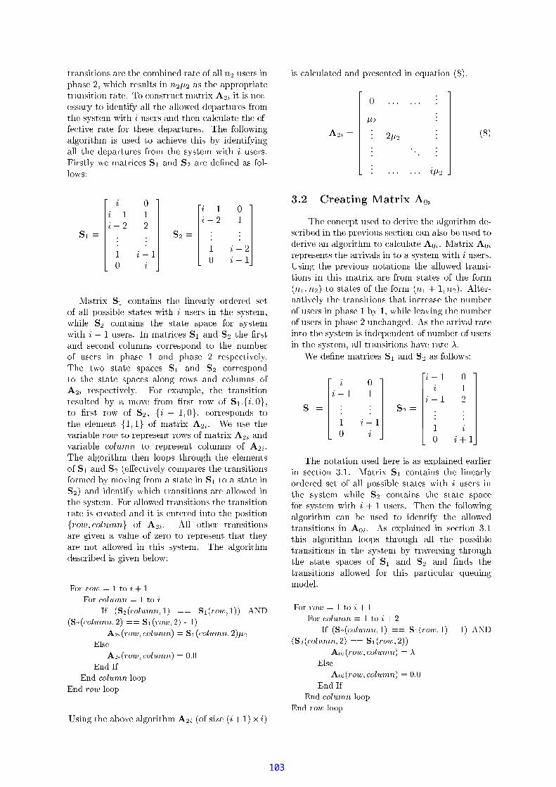
J=:`@_>AFGH J=H O>AF@_:=MxJ=a?M^UWOXZ?H >?MV+:`@\J=MO_N@_S S &I<AFGMT:`FRH >?aA@FGM$ÀLoLg^a?H[U`ai:=MVFG<?S J`FH >&I _ I@FJ=a?M$@_??:=O?:=H[@\J=MJ=:`@_>AFGH J=H O>Y:`@\J=MQRO+UWO>AFKJ=:=<AU®JeXC@\J=:=H ¨ I'ZH JH[Fe>?MVU®MVF=F=@_:=DYJ=OYH[LMT>,J=H NPDi@_S SJ=a?M+@_S S O\gMVLMTA@_:GJ=<?:=MVFNP:=OXJ=a?MFGDLFKJ=MTX g^H J=a |e<AFGMT:`F@_>ACJ=a?MT>iUT@_S[UW<?S[@\J=M;J=a?M(MWN NPMVU®J=H cM¡:`@\J=MNPO:YJ=a?MVFGMLMTA@_:GJ=<?:=MVFT¤Qa?MiNPOS S O\g^H >?@_S O:=H J=a?XÇH[F1<AFGMV¤J=O8@U`a?H MTcMiJ=a?H[F D8H[LMT>,J=H NPD H >?@_S SxJ=a?MLMTA@_:GJ=<?:=MVF(NP:=OX J=a?MFGDLFKJ=MTX g^H J=a |<AFGMT:`FTÛ£H :`FKJ=S DigMZXC@\J=:=H[UWMVFH$@_>A&I+@_:=MZLMW¯A>?MV¢@F^NPOS S O\g;FTp

HJ

| m| ] ½ ½| ] À À ½ | ] ½m |

&IJ

| ] ½ m| ] À ½ ½ | ] Àm | ] ½

f @\J=:=H ¨H8UWO>,J`@_H >AF¢J=a?MS H >?MV@_:=S DO:`LMT:=MVÅFGMWJO_N;@_S S O,F=FGH ?S MFKJ`@\J=MVF+g^H J=ao|(<AFGMT:`F$H >¦J=a?MiFGDLFKJ=MTX¡og^a?H S M&I6UWO>,J`@_H >AFJ=a?MlFKJ`@\J=MlFGA@UWMNPO:FGDLFKJ=MTXg^H J=ak| ] ½+<AFGMT:`FT I >¢XC@\J=:=H[UWMVFH$@_>A&I+J=a?MZ¯A:`FKJ@_>A7FGMVUWO>A7UWOS <?XY>AFUWO:=:=MVFG O>A.J=O¤J=a?M¦> <?XZ MT:O_N¢<AFGMT:`FH > ?aA@FGMl½7@_>A ?aA@FGMÀ:=MVFG MVU®J=H cMTS DQa?MÄJKgOØFKJ`@\J=M FGA@UWMVFHÅ@_>A&I UWO:=:=MVFG O>AJ=O¤J=a?M¦FKJ`@\J=M¦FGA@UWMVF¡@_S O>?¤:=O\g;F¡@_>A7UWOS <?XY>AF¡O_N I'Z¢:=MVFG MVU®J=H cMTS DÛ?O:MW¨?@_XY?S Mo1J=a?M.J=:`@_>AFGH J=H O>:=MVFG<?S J=MV7 D@XYO\cMNP:=OX ¯A:`FKJ¢:=O\gÃO_N HEo |F=ms,oJ=Ol¯A:`FKJ:=O\g O_N&Io | ] ½GF=ms,o¡UWO:=:=MVFG O>A?F¦J=OJ=a?MMTS MTXYMT>,J ½GFT½8O_NXC@\J=:=H ¨ I'ZG ©M<AFGMJ=a?Mc\@_:=H[@_?S M7J=O:=MT?:=MVFGMT>,J:=O\g;FO_NRXC@\J=:=H ¨ I'Ze@_>Ac\@_:=H[@_?S M9 J=OÅ:=MT?:=MVFGMT>,JUWOS <?XY>AF8O_N I'ZGQa?M¢@_S O:=H J=a?XÏJ=a?MT>S O OAFJ=a?:=O<?a8J=a?M¢MTS MTXYMT>,J`FO_NH^@_>A &I MBMVU®J=H cMTS DCUWOXYA@_:=MVFJ=a?M;J=:`@_>AFGH J=H O>AFNPO:=XYMVC DXYO\c H >?$NP:=OX @ZFKJ`@\J=M;H >HJ=O@+FKJ`@\J=MH >&IV@_>AH[LMT>,J=H NPD¡g^a?H[U`aJ=:`@_>AFGH J=H O>AF@_:=M@_S S O\gMViH >J=a?M(FGDLFKJ=MTX¡Û?O:@_S S O\gMVZJ=:`@_>AFGH J=H O>AFJ=a?M;J=:`@_>AFGH J=H O>:`@\J=M+H[FUW:=MV@\J=MV@_>A¡H J(H[FMT>,J=MT:=MV¡H >,J=OCJ=a?MZ O,FGH J=H O> F9dÄO_N I'ZG9;S SO_J=a?MT:J=:`@_>AFGH J=H O>AF@_:=MH cMT>8@c\@_S <?MiO_NbaTMT:=OJ=O:=MT?:=MVFGMT>,JZJ=aA@\JJ=a?MTD@_:=M¢>?O_J@_S S O\gMV¤H >J=a?H[F¡FGDLFKJ=MTX¡ÄQa?M@_S O:=H J=a?XLMVF=UW:=H MVH[F^H cMT>i MTS O\g$p

0 ! @ #" " @0$&% ')( @ #"*,+ ?.- ? $&% ')( @BA ` - ? ! @BA%A0/2143?.- ? $&% ')( 65 A ` - ? ! 65 A87 @BA"* 0/ ? ! 9$&% ')( 9A - ? $&% ')( 65 A ' 1 "* 0/ ? ! 9$&% ')( 9A +):*,+

+):$&% ')( *+): ! *

b FGH >?J=a?M@_ O\cM^@_S O:=H J=a?X I'Z O_NFGH aTM |G½E<;|K

H[F;UT@_S[UW<?S[@\J=MVi@_>A?:=MVFGMT>,J=MVH >¡MV§,<A@\J=H O> ,= ®

I'ZJ

m 555 555_ I À _ I 555 555 | _ I

,=

e;:qÊ Ò´?ÌÓ£³?¹G²;Í ÎÏÓ£³L´A¹<>=?>AQa?MUWO>AUWMTLJ<AFGMVCJ=OYLMT:=H cM;J=a?M$@_S O:=H J=a?X LMW

F=UW:=H MVH >J=a?M^?:=MTc H O<AFFGMVU®J=H O>CUT@_>Y@_S[FGO M^<AFGMVZJ=OLMT:=H cM@_>i@_S O:=H J=a?X J=OCUT@_S[UW<?S[@\J=M EZG f @\J=:=H ¨ EZ:=MT?:=MVFGMT>,J`F£J=a?M@_:=:=H c\@_S[FH >J=OZ@$FGDLFKJ=MTXÅg^H J=a$|R<AFGMT:`FTb FGH >?J=a?M1?:=MTc H O<AF$>?O_J`@\J=H O>AFJ=a?M@_S S O\gMVJ=:`@_>AFGH J=H O>AFH >J=a?H[FXC@\J=:=H ¨@_:=M1NP:=OX FKJ`@\J=MVFZO_N;J=a?MNPO:=X HF5&IVJ=OFKJ`@\J=MVF^O_NeJ=a?M$NPO:=X H ½GF5&IT®;9;S J=MT:G>A@\J=H cMTS DCJ=a?MJ=:`@_>AFGH J=H O>AFJ=aA@\J;H >AUW:=MV@FGM(J=a?M$> <?XZ MT:O_N<AFGMT:`FH >C?aA@FGM$½^ D½og^a?H S M;S MV@Ec H >?(J=a?M;> <?XZ MT:O_N<AFGMT:`FeH >C?aA@FGMÀ(<?>AU`aA@_>?MV9FeJ=a?M@_:=:=H c\@_SL:`@\J=MH >,J=O$J=a?MFGDLFKJ=MTXÄH[FeH >ALMT MT>ALMT>,JO_N> <?XZ MT:O_N<AFGMT:`FH >iJ=a?M+FGDLFKJ=MTX¡o?@_S SJ=:`@_>AFGH J=H O>AFaA@EcM:`@\J=M C ©M+LMW¯A>?M$XC@\J=:=H[UWMVF@H(@_>A&I$@FNPOS S O\g;FTpHJ

| m| ] ½ ½ ½ | ] ½m |

&IJ

|:.½ m| ½| ] ½ À ½ |m |:.½

Qa?M+>?O_J`@\J=H O><AFGMV¡a?MT:=M$H[F@F^MW¨L?S[@_H >?MV¡MV@_:=S H MT:H >FGMVU®J=H O>É? ½ f @\J=:=H ¨AHUWO>,J`@_H >AFCJ=a?MS H >?MV@_:=S DO:`LMT:=MV¦FGMWJYO_N(@_S S O,F=FGH ?S MiFKJ`@\J=MVFZg^H J=a|$<AFGMT:`F+H >J=a?M6FGDLFKJ=MTX"g^a?H S MB&I7UWO>,J`@_H >AFJ=a?MFKJ`@\J=MFGA@UWMNPO:FGDLFKJ=MTX g^H J=ao|d6½C<AFGMT:`FT¢Qa?MT>J=a?M1NPOS S O\g^H >?@_S O:=H J=a?X UT@_>Ä M<AFGMVlJ=OH[LMT>,J=H NPDlJ=a?M.@_S S O\gMVJ=:`@_>AFGH J=H O>AF1H > EZKÅ9FMW¨L?S[@_H >?MVH >FGMVU®J=H O>É? ½J=a?H[F6@_S O:=H J=a?X S O OAFJ=a?:=O<?a @_S SJ=a?M O,F=FGH ?S MJ=:`@_>AFGH J=H O>AFCH >.J=a?MFGDLFKJ=MTX D8J=:`@EcMT:`FGH >?J=a?:=O<?aJ=a?M6FKJ`@\J=MFGA@UWMVF¤O_NCH@_>AD&I@_>AƯA>A?F8J=a?MJ=:`@_>AFGH J=H O>AF@_S S O\gMV NPO:¤J=a?H[FA@_:GJ=H[UW<?S[@_:.§,<?MT<?H >?XYOLLMTSq0 ! @ #" " @

02$&% ')( @ #" "E5*,+ ?.- ? $&% ')( @BA ` - ? ! @BA " @BAF/2143?.- ? $&% ')( 65 A ` - ? ! 65 A%A"%/ ? ! 9$&% ')( 9A 1 "%/ ? ! 9$&% ')( 9A +):*,+

+):$&% ')( *+): ! *

b FGH >?+J=a?H[F@_S O:=H J=a?XÄXC@\J=:=H ¨ EZ O_NRFGH aTM |s¦½E8; |:8ÀGUT@_>i M$H cMT>¡@FNPOS S O\g;FTp

EZJ C 555 555

555 C m

n,

e;:+e Ò´?ÌÓ£³?¹G²;Í ÎÏÓ£³L´A¹<>=A H,ZC:=MT?:=MVFGMT>,J`Fi@_S SJ=a?MJ=:`@_>AFGH J=H O>AFig^a?H[U`aLO

>?O_J$U`aA@_>?M+J=a?M> <?XZ MT:O_N<AFGMT:`FTo |`o H >¢J=a?MCFGDLFKJ=MTX¡o>A@_XYMTS D(J=a?M?aA@FGMU`aA@_>?MVFR@_>AJ=a?MFGMTS N qJ=:`@_>AFGH J=H O>AFTb FGH >?1J=a?MZ?:=MTc H O<AF;>?O_J`@\J=H O>AFToAJ=a?M@_S S O\gMViJ=:`@_>AFGH J=H O>AFH >J=a?H[FiXC@\J=:=H ¨@_:=MNP:=OX FKJ`@\J=MVF HF5&IVCJ=O H ] ½GF5&I:½Ee@_>ANP:=OX HF5&IV£J=O HF5&IV®eQa?M:`@\J=MNPO:iJ=a?M¦?aA@FGMJ=:`@_>AFGH J=H O>AF¡@_:=MH cMT> DJ=a?MUWOXZ?H >?MV¦:`@\J=M1O_NHC<AFGMT:`F+H >¦J=a?M¯A:`FKJ?aA@FGM1 MWNPO:=MJ=a?M$J=:`@_>AFGH J=H O>AFTQa?M+FGMTS N qJ=:`@_>AFGH J=H O>¡:`@\J=MVF;UT@_> MNPO<?>A+MV@FGH S D$ D$OAFGMT:=c H >?^J=aA@\Jx@_S S,J=a?M:=O\gFG<?XCF@_:=M!aTMT:=OZNPO:;@_> DÆXC@\J=:=H ¨¼ kE¾¿Qa?MNPOS S O\g^H >?¦@_S O:=H J=a?XÇUT@_> M¢<AFGMV8J=OUW:=MW

@\J=M$@_S SJ=a?M$MTS MTXYMT>,J`FMW¨?UWMTLJ^J=a?M+LH[@_O>A@_SMTS MTXYMT>,J`FO_N H,ZGQa?MLH[@_O>A@_SMTS MTXYMT>,J`F(@_:=M$H >?H J=H[@_S S D¡H cMT>aTMT:=OH >J=a?H[F;@_S O:=H J=a?X¡Qa?MT>iJ=a?M$UWO:=:=MVU®J^LH[@_O>A@_SMTS MTXYMT>,J`F^ MVUWOXYMJ=a?M$>?MT,@\J=H cMO_N:=O\g7FG<?XCF^O_N£J=a?M XC@\J=:=H ¨@FJ=a?M1:=O\g FG<?XCF+@_:=M$aTMT:=OiNPO:Z@_> D:`@\J=MJ=:`@_>AFGH J=H O>XC@\J=:=H ¨^©MLMW¯A>?M+XC@\J=:=H[UWMVF#H$@_>AE&I@FZNPOS S O\g;FZJ=OOLJ`@_H >@_S SJ=a?M¡MTS MTXYMT>,J`FYMW¨?UWMTLJYJ=a?MLH[@_O>A@_SMTS MTXYMT>,J`F^O_N H,ZG

HJA&IJ

| m| ] ½ ½ ½ | ] ½m |

f @\J=:=H ¨ H@_>A &IUWO>,J`@_H >YJ=a?M;S H >?MV@_:=S DO:`LMT:=MVYFGMWJO_N;@_S S O,F=FGH ?S MFKJ`@\J=MVF+g^H J=ao|(<AFGMT:`F$H >¦J=a?MiFGDLFKJ=MTX¡Qa?MT>o0 ! @ #" " @

0$&% ')( @ #" " @*,+ ?.- ? $&% ')( @BA ` - ? ! @BA & @BAF/2143?.- ? $&% ')( 65 A ` - ? ! 65 A " @BA"$1/ ? ! 9$&% ')( 9A - ? ! @BA '& 1 "$1/ ? ! 9$&% ')( 9A +):*,+

+):$&% ')( *+): ! *

Qa?M+LH[@_O>A@_SMTS MTXYMT>,J`F^@_:=MH cMT> Dp

] EZ9 H,Z9 I'Z¿ Fg^a?MT:=M :=MT?:=MVFGMT>,J`F(J=a?MC:=O\gÄFG<?X O_NJ=a?M1A@_:GJ=H[UW<?S[@_:ZXC@\J=:=H ¨ H,Z O_NFGH aTM | 6½E; | 6½EG$H[F

H cMT>iH >¡MV§,<A@\J=H O> ½Vm,®

"$1/

&@"'& & ? " & @BA '&P... . . . . . .& ? " & A '&. . . . . .&/ 79 '&... &/

< ============>?0@ Ag^a?MT:=M(NPO:$Jm FT½GF F5| J C | ] ? _ H _ I ½½E

Á;O\gMTcMT:VoL<?M;J=O$J=a?MMW¨ J=:`@ O<?>A?@_:=DYUWO>ALH J=H O>?:=MVFGMT>,J$g^a?MT>J=a?MC> <?XZ MT:+O_N<AFGMT:`FH >J=a?M1FGDLFKJ=MTXH[F1MV§,<A@_S^J=O¦J=a?M¢> <?XZ MT:1O_N+FGMT:=cMT:`FTo FYNPO:)Jm FT½GF555BF5H >J=a?MXC@\J=:=H ¨ HaA@EcMJ=OY MXYOLLH ¯AMV@FNPOS S O\g;FTp

J | ] ? _ H _ I ½EÀ

p³LÓ£³?¹Kµ²;Ó´! ´?µ zÓdz(¹GÐG¹¬³?¹KÌRÚµxÑܳ?Ù;Ìp";Ú³LÌ$#d MVU®J=H O>AF(É? ½$^É? É1MW¨L?S[@_H >?MVa?O\g7J=O¡UW:=MV@\J=MZ@_S S

J=a?M8FG<?XC@\J=:=H[UWMVF¡:=MV§,<?H :=MVJ=O.MT>?MT:`@\J=MJ=a?M¦:`@\J=MJ=:`@_>AFGH J=H O>ÅXC@\J=:=H ¨Å:=MT?:=MVFGMT>,J=H >?J=a?Mª «­?:=OLUWMVF=Fg^H J=aiMT>?MT:`@_S H[FGMV¥x:=S[@_>?FGMT:=c H[UWMLH[FKJ=:=H ?<LJ=H O>Qa?MO MVU®J=H cM+O_NeJ=a?H[FFKJ=<ALD¡H[F;J=O¡@_>A@_S DLFGM+J=a?MZ MT:GNPO:=XC@_>AUWM+O_N@1UWMTS S <?S[@_:(>?MWJKgO:=jo?NPOLUW<AFKH >?O>ZJ=a?M^?S OLU`j H >?(?:=OA@_?H S H J=H MVF£NPO:aA@_>ALO\cMT:e@_>A>?MTg <AFGMT:`F+@F$J=a?MXC@_H > MT:GNPO:=XC@_>AUWM1@_>A@_S DLFGH[F$A@\:`@_XYMWJ=MT:VQRO¡UT@_S[UW<?S[@\J=MZJ=a?MY?S OLU`j H >?i?:=OA@_?H S H J=H MVFToH J^H[F>?MVUWMVF=F=@_:=DJ=O¯A>AJ=a?M$FKJ`@\J=H O>A@_:=DY?:=OA@_?H S H J=H MVFO_NJ=a?M1FGDLFKJ=MTX¡ I >O_J=a?MT:gO:`?FJ=a?MC?:=OA@_?H S H JKDO_NaA@Ec H >?*|<AFGMT:`FH >iJ=a?M+FGDLFKJ=MTX¡oLg^H J=a|x:`@_>?H >?ZNP:=OXmJ=O$eo?>?MTMViJ=OC M$NPO<?>AQa?M$?aA@FGMWqJKD M+FGMT:=c H[UWMLH[FKJ=:=H ?<LJ=H O>CH >,J=:=OLL<AUWMVF |G½&%')(%*,+-*,.%£g^H J=a?H >CMV@U`aO_NJ=a?MVFGM^|(FKJ`@\J=MVFT I >J=a?H[FZFGMVU®J=H O>¦gMCg^H S S?:=MVFGMT>,JXYMWJ=a?OL?FJ=OiUT@_S[UW<?S[@\J=M+J=a?MYFKJ`@\J=H O>A@_:=Di?:=OA@_?H S H J=H MVFUWO:=:=MVFG O>ALH >?(J=OZ@_S S?J=a?M(FG<?1FKJ`@\J=MVF@_>AJ=a?MT>1FGa?O\ga?O\g gM¢UT@_>.UWOXZ?H >?MiJ=a?MVFGMFG<?.FKJ`@\J=M¢FKJ`@\J=H O>A@_:=D?:=OA@_?H S H J=H MVF(J=O¢UT@_S[UW<?S[@\J=MJ=a?M1?:=OA@_?H S H JKD¢O_N¯A>A H >?|<AFGMT:`FH >iJ=a?M+FGDLFKJ=MTX @\J;@_> D1H >AFKJ`@_>AUWMQa?M:=MTS[@\J=H O>AFGa?H MWJKgMTMT> J=a?M7FKJ`@\J=H O>A@_:=DlO:

MV§,<?H S H ?:=H <?XÏ?:=OA@_?H S H J=H MVF@_>AJ=a?Mi:`@\J=M1J=:`@_>AFGH J=H O>XC@\J=:=H ¨CNPO:@+J=H XYMW¿a?OXYOMT>?MTO<AFO>,J=H > <?O<AFQH XYMf @_:=jO\cZaA@_H > Q f £H[FeH cMT>Z D+MV§,<A@\J=H O> ½VÉ,®I JaA@F£ MTMT>YFGa?O\g^>+H >i¼ kE¾ J=aA@\JMV§,<A@\J=H O> ½VÉ,H[F£c\@_S H[NPO:(@1g^H[LMZc\@_:=H MWJKDO_NFGDLFKJ=MTXCF;H > cOS c H >?CJKD MWqJKD MLH[FKJ=:=H ?<LJ=H O>AFTQa?M FKJ`@\J=H O>A@_:=D LH[FKJ=:=H ?<LJ=H O>!cMVU®J=O:Vo0/ J1 2 HF 2 IGF:F 243-57698: o;NPO:¡@_>)6§,<?MT<?H >?

FGDLFKJ=MTX F=@\J=H[FK¯AMVFTo

/J U F 2 Z<;¤m F 3-57698 Z =H 2 ZJ6½ ½VÉ,

¥§,<A@\J=H O> ½VÉ,£FKJ`@\J=MVF£J=aA@\JeJ=a?M^?:=OA@_?H S H JKDÂAO\g;FH >,J=O+@_> DZFKJ`@\J=M^H[FeA@_S[@_>AUWMV D+J=a?M^?:=OA@_?H S H JKD$ÂAO\g;FO<LJO_NxJ=aA@\J$FKJ`@\J=M$Û?O:@iFGDLFKJ=MTXØg^H J=ak8U`aA@_>?>?MTS[FToJ=a?MFGH aTM(O_NJ=a?MJ=:`@_>AFGH J=H O>:`@\J=MXC@\J=:=H ¨ H[F 8H ; 8Hg^a?MT:=Mo

J Z =H | J .½EÀ 5 ½TÈ

Qa?MZUWOXY?<LJ`@\J=H O>A@_SRUWOXY?S MW¨LH JKDCNPO:^¯A>ALH >?CJ=a?MFKJ`@\J=H O>A@_:=DLH[FKJ=:=H ?<LJ=H O>cMVU®J=O:O_N+J=a?MFGDLFKJ=MTX H >LUW:=MV@FGMVFg^H J=aZJ=a?M^FGH aTMO_N:¡d,J=OLU`aA@FKJ=H[UUWOXY?S MTXYMT>LJ`@\J=H O>?:=O\c H[LMVF^@1UWOXY?<LJ`@\J=H O>A@_S S DiU`a?MV@_ MT:;XYMVU`aL@_>?H[FGXJ=O8FGOS cM¥§,<A@\J=H O> ½VÉ,C DLMVUWO<??S H >?¤@_>H :=:=MVL<AUWH ?S MS[@_:=M f @_:=jO\c+U`aA@_H >o_:=MT?:=MVFGMT>,J=MVZ D$¡oH >,J=OCFGXC@_S S MT:^H :=:=MVL<AUWH ?S M f @_:=jO\cCU`aA@_H >AF$¼ c ¾¿º >AUWM¡J=a?MFKJ`@\J=H O>A@_:=D?:=OA@_?H S H J=H MVFYO_NJ=a?M¢FGDLFK

J=MTX¡o"/eoaA@EcM¡ MTMT>¤OLJ`@_H >?MV¤FG<AU`a8J=aA@\J / 5 J ½og^a?MT:=MYH[F@ZUWOS <?XY>cMVU®J=O:O_Nx½ FTo gM(UT@_>1¯A>ACJ=a?M?:=OA@_?H S H JKDO_NRaA@Ec H >?|<AFGMT:`FxH >1J=a?MFGDLFKJ=MTX |Kx@FNPOS S O\g;FTp

m, J 2 ½E |K J 3 H,&Z

= 3 H 2 NPO: | ;7½ ½Ek

@_>A:ZeH[F^@F^LMW¯A>?MVi MWNPO:=MH >¡MV§,<A@\J=H O> ½TÈ ®I NLJ=a?MFGDLFKJ=MTX6LO MVF>?O_JLH[FKJ=H >?<?H[FGa+ MWJKgMTMT>$>?MTg

@_>AaA@_>ALO\cMT:<AFGMT:`F>?O;?:=H O:=H JKDg^H S S, MH cMT>J=O;O>?MUWS[@F=FO\cMT:J=a?MO_J=a?MT:V I >ZFG<AU`aZ@FGDLFKJ=MTX7J=a?M?S OLU`j H >??:=OA@_?H S H JKDCNPO:;@_> DC<AFGMT:Vo oLg^H S S M$H cMT>i Do J R ½ \ @_>A¤J=a?M@EcMT:`@_MiS O,@O_NJ=a?MFGDLFKJ=MTX¡o;o;@\J1J=a?H[F?S OLU`j H >?Y?:=OA@_?H S H JKDCH[F^H cMT>i D

J Z =H | |K ½ c Òµ²¸ÐG·Ú ¹Kµ²Ú9UTUW<?:`@\J=MXYMWJ=a?OL?FxaA@EcM MTMT>1LMT:=H cMV+J=OXYOLLMTS

UWMTS S <?S[@_:(>?MWJKgO:=jLFH >:=MVUWMT>,JJ=H XYMVFC¼ = onE¾¿ZÁ;O\gMTcMT:L<?MJ=OJ=a?MTH :xUWOXY?S MW¨LH JKDo_J=a?MVFGM^XYOLLMTSALO>?O_Jx:=MVFG<?S JH >J=:`@U®J`@_?S M+§,<?MT<?H >?iFGDLFKJ=MTXCFT I >¼ ÀE¾£gMZ?:=O O,FGMVJ=O+XYOLLMTSAJ=a?M(U`aA@_>?>?MTSAa?OS[LH >?$J=H XYMH >UWMTS S <?S[@_:x>?MWJGgO:=jLFxg^H J=ai@À$?aA@FGMMT>?MT:`@_S H[FGMVC¥x:=S[@_>?ZLH[FKJ=:=H ?<LJ=H O>©M(FGa?O\gMVJ=aA@\JJ=a?H[FLH[FKJ=:=H ?<LJ=H O>@UTUW<?:`@\J=MTS D@_??:=OE¨LH XC@\J=MVFJ=a?MLH[FKJ=:=H ?<LJ=H O>¢O_NU`aA@_>?>?MTSRa?OS[LH >?J=H XYM+H >@CUWMTS S <?S[@_:^>?MWJKgO:=j I >¡J=a?H[F^A@_ MT:;gM$<AFGMVFGOXYMC?:=O MT:GJ=H MVF$O_NJ=a?M1MT>?MT:`@_S H[FGMV¥x:=S[@_>?LH[FKJ=:=H ?<LJ=H O>¤J=OLMT:=H cM¡@¦FGH XY?S H ¯AMV§,<?MT<?H >?¦FGDLFKJ=MTX J=OXYOLLMTS£J=a?MCUWOS S MVU®J=H cMU`aA@_>?>?MTS[FO_N@iUWMTS SH >UWMTS S <?S[@_:>?MWJKgO:=jLFTQa?MVFGMFGH XY?S H ¯ UT@\J=H O>AFMT>A@_?S MV1<AFJ=OCLMW:=H cM@1J=:`@U®J`@_?S M§,<?MT<?H >?iXYOLLMTSNP:=OX»@iFGMTMTXYH >?S D<?>,J=:`@U®J`@_?S M ª «­Z©M1J=a?MT>8?:=MVFGMT>,J=MVJ=a?MXYMWJ=aLOL?F<AFGMVJ=O¤UT@_S[UW<?S[@\J=M¢J=a?M?S OLU`j H >??:=OA@_?H S H J=H MVF

NPO:aA@_>ALO\cMT:@_>AC>?MTg<AFGMT:`FT­<?M(J=OFGA@UWM(S H XYH J`@\J=H O>AFO_NeJ=a?MA@_ MT:VogM+O>?S D¡?:=MVFGMT>,J=MV¡J=a?MYFGH XY?S H ¯ UT@\J=H O>CJ=MVU`a?>?H[§,<?MVFxgM<AFGMVYH >1J=a?H[FFKJ=<ALDJ=aA@\JUT@_> M^@_??S H MV+J=O$FGH XYH S[@_:e?:=O?S MTXCFT I >,J=MT:=MVFKJ=MV+:=MV@LMT:`FFGa?O<?S[:=MWNPMT:J=O¢¼ ÀV¾£@_>A¼ ÉE¾NPO:¯A>A@_S:=MVFG<?S J`FT ÌÑ`Ì´?ÌR²¸ÌRÚ¼ ½W¾+¥;;­Z]^Mo$]$;ÛA@_>,J`@UTUWHqo@_>A((H[@_XC@_ MT>?Mo

Á@_>ALO\cMT:+@_>A­D >A@_XYH[UiaA@_>?>?MTS9;S S OLUT@\J=H O>QRMVU`a?>?H[§,<?MVF H > f O?H S M MTS S <?S[@_: ;MWJKgO:=jLFTo + %"!$# .&%'! .&(&%) +*, ! ocOSqÈÈAo+>?OAÀLo?AÉn c"- È,m,kLo ½Vnn,kL

¼ ÀE¾+9+£B,@ED,@FG<?:=H D,@?oBAR9FGMT>AFKJ=O:GNPMT:VoR@_>A­Z(:=MTMT>o f OLLMTS S H >?Zd MT:=c H[UWM^QH XYM;­H[FKJ=:=H ?<LJ=H O>AFxH >MTS S <?S[@_:;;MWJKgO:=jLF b FGH >? aA@FGMW¬QD M;FGMT:=c H[UWM(­H[FKJ=:=H ?<LJ=H O>AFTo H >/. *0(0! )*1!32* 045!* 62*787 ' :9<;(+-*=9* %®o Á;MTS[FGH >?j HqoAÛ£H >?S[@_>AA®o B<?>?M+À_mm?½

¼ É\¾+9+ B,@ED,@FG<?:=H D,@?o 7> *?-.&@ A + +@B*?-. . . 45* 7 + +(. % *-'BCD% EF* (59<, 9 *=G . .5;@9(*=9* %® aA­ J=a?MVFGH[FTo b >?H cMT:`FGH JKDO_Nd O<LJ=a-9;<AFKJ=:`@_S H[@?o À_mm?½ b ];h H5II=JLK MNMPOQOQOR S I=TPR UDVDS WYX0R Z\[DULR X&U]MQX&T=UDVX5MJX&J]Z\T=W1MPI=HDZ\W=S WPR J][0^ ¼ È_¾ZdY9FGXZ<AF=FGMT>o º ;MT:=XC@_>o¡@_>A f º S[F=FGO>o Û£H JGJ=H >? aA@FGMWqJKD M­H[FKJ=:=H ?<LJ=H O>AFc H[@$J=a?M¥ f9;S O:=H J=a?X¡o `_a(+ +@9< 4+?09 + b*-' 4+,*\4_ *,+-*=9 %N;*=9(%®o?cOSqAÀ_É?oL??ÈA½Vn - ÈÈA½oA½Vnn \

¼ kE¾ f ;MT<LJ`FTocE +-* 9 dB;Ne .&*7 .* 9(f_a*, '*=9* %g9< _ *1*0(&% + %*=9(hEF*0@ .5, %®BOa?>Á;O?j H >AF <??S H[FGa?MT:`FTo½Vn = ½

¼ \ ¾jiZ @_O<?XYO\co b 8k:=H MTMT:Vo@_>A ­ZZ©@_>?MT:Vo 9;>A@_S DLFGH[FO_N£@ f <?S J=H[FGMT:=cMT:­MTS[@ED,¬hO,F=Fd DLFKJ=MTXg^H J=a@((MT>?MT:`@_S f @_:=jO\c H >A@^9;:=:=H c\@_S :=OLUWMVF=FTo ^H >½Dl76 )*,. 4+-*=9* 4+,j2* 045!m* nE +-* 9 dB;=op 4+, G-*=9(+,E .*q%'*0@ %sr=EtoEvuh9< /_ *1*0(&% + %*=9(mEF*0@ .5, %®

¼ c ¾+9+eB,@ED,@FG<?:=H D,@i@_>AwkY­Oyx,@_>zUT@EDo d,J=OLU`aA@FKJ=H[UOXY?S MTXYMT>,J`@\J=H O>¦9;??S H MVJ=O¡J=a?M19;>A@_S DLFGH[F$O_N«S OLU`j H >? :=OA@_?H S H J=H MVF;H >¦MTS S <?S[@_: ;MWJKgO:=jLFTo H >|. *0(0! o_ +~ )*,. 4+-*=9* 4+,s2* 04. .5 +(.N 9 .5, .%% + +@>4*=9(+,2*787 ' :9(+-*=9* Ao «@_>so9;S MT:GJ`@?o@_>A@?@,®o?B<?S DiÀ_mm,ÀL

¼ = ¾ º :=S H jÄ@_>AÆd];@_?A@_ O:GJVo 9 f OLLMTS1NPO:QRMTS MWJ=:`@\1U MT:GNPO:=XC@_>AUWM@_>AØaA@_>?>?MTSÁ;OS[ H >?QH XYMaA@_:`@U®J=MT:=H aV@\J=H O>¢H >©.H :=MTS MVF=FZMTS S <LS[@_:$OXYXZ<?>?H[UT@\J=H O>¡g^H J=a(MT>?MT:`@_S£d MVF=FGH O>¢@_>A­gMTS SQH XYM1­H[FKJ=:=H ?<LJ=H O>AFTo b!_ .5, .&(*,.&@o .+ %2*787 ' +! ocOSq;½ \ o? c= =D- = mÉ?oB<?>?M½Vnn =

¼ n\¾ÛA@_>?¡@_>A I Ra?S[@_X+J`@U_o QRMTS MWJ=:`@\1UZ9;>A@_S D,FGH[Fe@_>A f O?H S H JKD f OLLMTS S H >?O_N d ;MWJKgO:=jLFTo + %"!2*787 ' +! oYcOSq(È c o?Y½Vm \ À -½Vm c ÀLoLB<?S D¢½Vnnn?

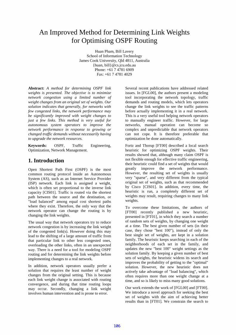
An Improved Method for Determining Link Weightsfor Optimising OSPF Routing

Huan Pham, Bill LaverySchool of Information Technology

James Cook University, Qld 4811, Australiahuan, bill@cs.jcu.edu.auPhone: +61 7 4781 6909

Fax: +61 7 4781 4029

Abstract: A method for determining OSPF linkweights is presented. The objective is to minimizenetwork congestion using a limited number ofweight changes from an original set of weights. Oursolution indicates that generally, for networks withfew congested links, the network performance maybe significantly improved with weight changes tojust a few links. This method is very useful forautonomous system operators to improve thenetwork performance in response to growing orchanged traffic demands without necessarily havingto upgrade the network resources.

Keywords: OSPF, Traffic Engineering,Optimization, Network Management.

1. Introduction

Open Shortest Path First (OSPF) is the mostcommon routing protocol inside an AutonomousSystem (AS), such as an Internet Service Provider(ISP) network. Each link is assigned a weight,which is often set proportional to the inverse linkcapacity [CIS01]. Traffic is routed via the shortestpath between the source and the destination, or"load balanced" among equal cost shortest pathswhere they exist. Therefore, the only way that thenetwork operator can change the routing is bychanging the link weights.

The usual way that network operators try to reducenetwork congestion is by increasing the link weightof the congested link(s). However doing this maylead to the shifting of a large amount of traffic fromthat particular link to other less congested ones,overloading the other links, often in an unexpectedway. There is a need for a tool for modeling OSPFrouting and for determining the link weights beforeimplementing changes to a real network.

In addition, network operators usually prefer asolution that requires the least number of weightchanges from the original setting. This is becauseeach link weight change is associated with routingconvergence, and during that time routing loopsmay occur. Secondly, changing a link weightinvolves human intervention and is prone to error.

Several recent publications have addressed relatedissues. In [FGL00], the authors present a modelingtool incorporating the network topology, trafficdemands and routing models, which lets operatorschange the link weights to see the traffic patternsbefore actually implementing it in a real network.This is a very useful tool helping network operatorsto manually engineer traffic. However, for largenetworks, manual operation can become socomplex and unpredictable that network operatorscan not cope. It is therefore preferable thatoptimization be done automatically.

Fortz and Thorup [FT00] described a local searchheuristic for optimizing OSPF weights. Theirresults showed that, although many claim OSPF isnot flexible enough for effective traffic engineering,their heuristic could find a set of weights that wouldgreatly improve the network performance.However, the resulting set of weights is usuallyvery "sparse", and very different from the typicaloriginal set of weights, such as that recommendedby Cisco [CIS01]. In addition, every time, theheuristic is run, a completely different set ofweights may result, requiring changes to many linkweights.

To overcome these limitations, the authors of[FT00] recently published a new heuristic,presented in [FT01], in which they search a numberof random sets of weights, by changing one weightat a time. The best given number of sets (in theircase, they chose "best 100"), instead of only thebest single set of weights, are kept in a solutionfamily. The heuristic keeps searching in each of theneighborhoods of each set in the family, andupdates the new "best 100" weight settings as thesolution family. By keeping a given number of bestsets of weights, the heuristic widens its search andimproves the probability of getting to the "optimal"solution. However, the new heuristic does notactively take advantage of "load balancing", whichoften requires more than one weight change at atime, and so is likely to miss many good solutions.

Our work extends the work of [FGL00] and [FT00].We introduce a novel approach for seeking the bestset of weights with the aim of achieving betterresults than in [FT01]. We constrain the search to

allow just a small number of changes from anoriginal set of link weights. We allow more thanone link weight to change at a time to actively takeadvantage of "load balancing".

In section 2 we introduce an appropriate objectivefunction for the optimization process, then in thefollowing section, derive methods for solving forthe desired sets of weights. Section 4 presentsresults for an arbitrary network and section 5discusses their significance.

2. Optimization Objective Function

When attempting to optimise routing, it is verycommon to turn to maximum link utilization as theperformance measure, such as proposed in[WWZ01] and [FGL00]. The justification is thatthis will reduce the likelihood of the highestutilisation link becoming congested. However, theoptimization process may get stuck once themaximum utilization can not be further decreased,although other less congested parts can still befurther optimized. Even if the average linkutilization is used as a secondary optimizingobjective, this may not help because, in some cases,we have to increase the average link utilization tohelp reduce network congestion. For example, seethe Figure 1, where all the links have the capacityof 10Mbit/s and there is a demand of 6Mbit/sbetween Router1 and Router5. The load balancedsituation shown has average utilisation of 26.2%,and is "less congested" than would be the casewhere all traffic were routed R1-R4-R5, whereaverage utilisation would be 20% but R1-R4 wouldbe operating at undesirably high utilisation.

To overcome the limitation of using the maximumlink utilisation, we use a convex "cost" function ofthe link utilisation as the objective function, after[FT00] as in Figure 2. This cost function can beinterpreted as the penalty cost of sending anadditional unit of traffic via a link; the heavier thelink utilisation, the higher the cost to send a unit oftraffic via that link. The use of such a function

helps to deter routing traffic via those links that arealready heavily loaded, and encourage routingtraffic via lightly loaded links. The intention is thatthe resulting optimal routing will therefore result inmore even load distribution across the network.

To be able to compare the performance of ourweight setting search heuristic with that achievedby the search heuristic of [FT00], we reuse theirpiecewise linear cost function Φa (Figure 2). Theoptimal routing problem can be formalized asfollows, for the network cost function, Φ:

Minimize ∑∈

Φ=ΦAa

a al ))((

subject to:

=− =

=−

∑∑∈∈

otherwise

tyiftsD

syiftsD

Azyz

tszy

Ayxx

tsyx ff

0

),(

),(

),(:

),(),(

),(:

),(),(

∑×∈

=NNts

tsafal

),(

),()(

<−

≤<−

≤<−

≤<−

≤<−

≤≤

=Φ

)(/)(10/11)(3

16318)(5000

10/11)(/)(1)(3

1468)(500

1)(/)(10/9)(3

178)(70

10/9)(/)(3/2)(3

16)(10

3/2)(/)(3/1)(3

2)(3

3/1)(/)(0)(

acalforacal

acalforacal

acalforacal

acalforacal

acalforacal

acalforal

a

where ),(),(

tsyxf is traffic flow from source s to

destination t over link x-y.D(s,t) is traffic demand from s to t.l(a), and c(a) are traffic load and capacity of link a

Router1

Router2

Router3

2M/ 10M

2M/ 10M

2M/ 10M2M/ 10M

2M/ 10M

Router5Router4

6M/ 10M

Figure 1: Load balancing reduces congestion whileincreasing average utilisation.

NtsAaf tsa ∈∈≥ ,;0),(

Figure 2: Cost versus Load, assuming Capacity=1

0

1

2

3

4

5

0 0.2 0.4 0.6 0.8 1 1.2

Load

Co

st

In order to have a cost function that is independentof network topology and traffic demand, the abovecost function is further normalized by dividing by afactor of total cost of a lightly loaded network, Φo,

where ∑∑∈∈

== ΦΦAaAa

a alalo

)())(( and traffic

follows the minimum hop count paths.

Next we solve the network cost minimization forthree scenarios

• We calculate the minimum cost function,assuming traffic can be routed arbitrarily. Thisyields the "theoretical optimal routing" solution

• Assuming OSPF routing operation (and evenload splitting over equal cost paths), wedetermine the minimum cost function allowingfor an unlimited number of changes in the setof link weights. This yields the "OSPFoptimal" solution.

• As for the second scenario but restricting thenumber of changes to link weights, wedetermine the OSPF-m solution, where m is themaximum number of changes permitted in theset of link weights.

3. Solution Methods

The theoretical optimal routing solution

First we need the solution for the optimal routingproblem, stated above. Here "optimal generalrouting" is the idealised case where traffic streamscan be routed at will; this is of course not practicalfor OSPF routing, but it gives a lower bound bywhich we can judge just how good is a solution.

In [FT00], the authors solved the general routingproblem using linear programming. Morespecifically, the problem is solved by callingCPLEX via AMPL. However, linear programming[ROT79] requires that the cost function must beapproximated to piecewise linear functions. Thismakes it difficult to use an arbitrary gradual convexfunction as the objective function.

Instead, we use the flow-deviation algorithm of[KER93] to solve this theoretical optimal routingproblem. By doing this, we can define any costfunction we want, including that of Figure 2.

Solving for an unlimited number of weightchanges

It has been shown in [FT00] that, finding theoptimal OSPF weight setting is a NP hard problem.There is no algorithm that can guarantee thesolution to such problems can be found in areasonable time limit. We will reuse the localsearch heuristic (using a hashing table as a guide) tosolve this problem, as in [FT00].

Solving with limited number of weight changes.

To solve this problem, we propose a novel "loadbalancing limited change local search heuristic",which is an extension of that proposed in [FT00].Since we want the solution that requires no morethan a limited number of changes from the originaldefault setting, unlike [FT00], our search is onlydone within those settings not too far from theoriginal. More specifically, the search space onlyincludes weight settings that are less than m-weightchanges from the original one, where m is themaximum allowed number of weight changes. Thisis important in practice, for it minimises the taskdemanded of the AS operator, in responding toscenarios such as growth in network trafficdemand.

Typically we start with preset values for linkweights, often set according to Ciscorecommendation. We then search both solutionswith one weight change at a time, and solutionsinvolving "load balancing" (Figure 3), which mayrequire more than one weight change. We searchfor load balancing solutions across allsource/destination pairs, S-D, selected randomly.

Let w1, w2, … wn be the weights of the linksoriginating from the source S, and d1, d2, … dn bethe distance (sum of weights) from thecorresponding neighbor routers to the destinationD. To load balance between all paths between S-D,the new weights for those links originating from Sare determined as follows:

w’i = 1 + max d1, …, dn - di

This load balancing solution requires a maximumof n-weight changes. We keep track of the currentsolution distance, d, from the original weightsettings. When we search for load-balancingsolutions, we often need to change more than oneweight; here we only evaluate the solutions with thenumber of weight changes less than or equal to m -d, i.e. the remaining available number of changes.

Figure 3: Load balancing solution

S

w1 d2

w2

wn

d1

dn

D

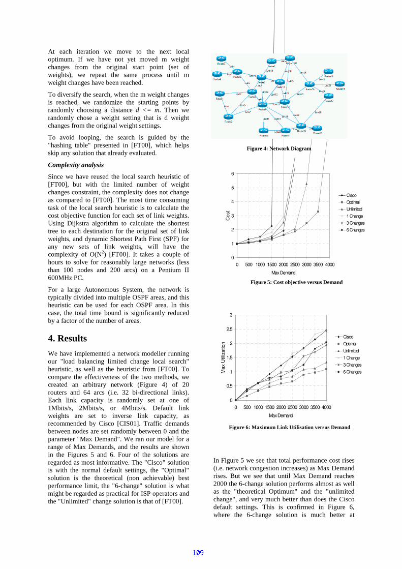
At each iteration we move to the next localoptimum. If we have not yet moved m weightchanges from the original start point (set ofweights), we repeat the same process until mweight changes have been reached.

To diversify the search, when the m weight changesis reached, we randomize the starting points byrandomly choosing a distance d <= m. Then werandomly chose a weight setting that is d weightchanges from the original weight settings.

To avoid looping, the search is guided by the"hashing table" presented in [FT00], which helpsskip any solution that already evaluated.

Complexity analysis

Since we have reused the local search heuristic of[FT00], but with the limited number of weightchanges constraint, the complexity does not changeas compared to [FT00]. The most time consumingtask of the local search heuristic is to calculate thecost objective function for each set of link weights.Using Dijkstra algorithm to calculate the shortesttree to each destination for the original set of linkweights, and dynamic Shortest Path First (SPF) forany new sets of link weights, will have thecomplexity of O(N2) [FT00]. It takes a couple ofhours to solve for reasonably large networks (lessthan 100 nodes and 200 arcs) on a Pentium II600MHz PC.

For a large Autonomous System, the network istypically divided into multiple OSPF areas, and thisheuristic can be used for each OSPF area. In thiscase, the total time bound is significantly reducedby a factor of the number of areas.

4. Results

We have implemented a network modeller runningour "load balancing limited change local search"heuristic, as well as the heuristic from [FT00]. Tocompare the effectiveness of the two methods, wecreated an arbitrary network (Figure 4) of 20routers and 64 arcs (i.e. 32 bi-directional links).Each link capacity is randomly set at one of1Mbits/s, 2Mbits/s, or 4Mbits/s. Default linkweights are set to inverse link capacity, asrecommended by Cisco [CIS01]. Traffic demandsbetween nodes are set randomly between 0 and theparameter "Max Demand". We ran our model for arange of Max Demands, and the results are shownin the Figures 5 and 6. Four of the solutions areregarded as most informative. The "Cisco" solutionis with the normal default settings, the "Optimal"solution is the theoretical (non achievable) bestperformance limit, the "6-change" solution is whatmight be regarded as practical for ISP operators andthe "Unlimited" change solution is that of [FT00].

In Figure 5 we see that total performance cost rises(i.e. network congestion increases) as Max Demandrises. But we see that until Max Demand reaches2000 the 6-change solution performs almost as wellas the "theoretical Optimum" and the "unlimitedchange", and very much better than does the Ciscodefault settings. This is confirmed in Figure 6,where the 6-change solution is much better at

0

0.5

1

1.5

2

2.5

3

0 500 1000 1500 2000 2500 3000 3500 4000

Max Demand

Max

Util

izat

ion

CiscoOptimalUnlimited1 Change3 Changes6 Changes

Figure 6: Maximum Link Utilisation versus Demand

0

1

2

3

4

5

6

0 500 1000 1500 2000 2500 3000 3500 4000

Max Demand

Cos

t

CiscoOptimalUnlimited1 Change3 Changes6 Changes

Figure 5: Cost objective versus Demand

Figure 4: Network Diagram

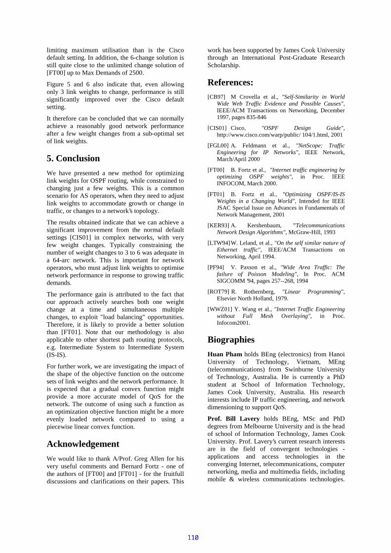
limiting maximum utilisation than is the Ciscodefault setting. In addition, the 6-change solution isstill quite close to the unlimited change solution of[FT00] up to Max Demands of 2500.

Figure 5 and 6 also indicate that, even allowingonly 3 link weights to change, performance is stillsignificantly improved over the Cisco defaultsetting.

It therefore can be concluded that we can normallyachieve a reasonably good network performanceafter a few weight changes from a sub-optimal setof link weights.

5. Conclusion

We have presented a new method for optimizinglink weights for OSPF routing, while constrained tochanging just a few weights. This is a commonscenario for AS operators, when they need to adjustlink weights to accommodate growth or change intraffic, or changes to a network’s topology.

The results obtained indicate that we can achieve asignificant improvement from the normal defaultsettings [CIS01] in complex networks, with veryfew weight changes. Typically constraining thenumber of weight changes to 3 to 6 was adequate ina 64-arc network. This is important for networkoperators, who must adjust link weights to optimisenetwork performance in response to growing trafficdemands.

The performance gain is attributed to the fact thatour approach actively searches both one weightchange at a time and simultaneous multiplechanges, to exploit "load balancing" opportunities.Therefore, it is likely to provide a better solutionthan [FT01]. Note that our methodology is alsoapplicable to other shortest path routing protocols,e.g. Intermediate System to Intermediate System(IS-IS).

For further work, we are investigating the impact ofthe shape of the objective function on the outcomesets of link weights and the network performance. Itis expected that a gradual convex function mightprovide a more accurate model of QoS for thenetwork. The outcome of using such a function asan optimization objective function might be a moreevenly loaded network compared to using apiecewise linear convex function.

Acknowledgement

We would like to thank A/Prof. Greg Allen for hisvery useful comments and Bernard Fortz - one ofthe authors of [FT00] and [FT01] - for the fruitfulldiscussions and clarifications on their papers. This

work has been supported by James Cook Universitythrough an International Post-Graduate ResearchScholarship.

References:

[CB97] M Crovella et al., "Self-Similarity in WorldWide Web Traffic Evidence and Possible Causes",IEEE/ACM Transactions on Networking, December1997, pages 835-846

[CIS01] Cisco, "OSPF Design Guide",http://www.cisco.com/warp/public/ 104/1.html, 2001

[FGL00] A. Feldmann et al., "NetScope: TrafficEngineering for IP Networks", IEEE Network,March/April 2000

[FT00] B. Fortz et al., "Internet traffic engineering byoptimizing OSPF weights", in Proc. IEEEINFOCOM, March 2000.

[FT01] B. Fortz et al., "Optimizing OSPF/IS-ISWeights in a Changing World", Intended for IEEEJSAC Special Issue on Advances in Fundamentals ofNetwork Management, 2001

[KER93] A. Kershenbaum, ”TelecommunicationsNetwork Design Algorithms", McGraw-Hill, 1993

[LTW94]W. Leland, et al., "On the self similar nature ofEthernet traffic", IEEE/ACM Transactions onNetworking, April 1994.

[PF94] V. Paxson et al., "Wide Area Traffic: Thefailure of Poisson Modeling", In Proc. ACMSIGCOMM ’94, pages 257--268, 1994

[ROT79] R. Rothernberg, "Linear Programming",Elsevier North Holland, 1979.

[WWZ01] Y. Wang et al., "Internet Traffic Engineeringwithout Full Mesh Overlaying", in Proc.Infocom2001.

Biographies

Huan Pham holds BEng (electronics) from HanoiUniversity of Technology, Vietnam, MEng(telecommunications) from Swinburne Universityof Technology, Australia. He is currently a PhDstudent at School of Information Technology,James Cook University, Australia. His researchinterests include IP traffic engineering, and networkdimensioning to support QoS.

Prof. Bill Lavery holds BEng, MSc and PhDdegrees from Melbourne University and is the headof school of Information Technology, James CookUniversity. Prof. Lavery’s current research interestsare in the field of convergent technologies -applications and access technologies in theconverging Internet, telecommunications, computernetworking, media and multimedia fields, includingmobile & wireless communications technologies.

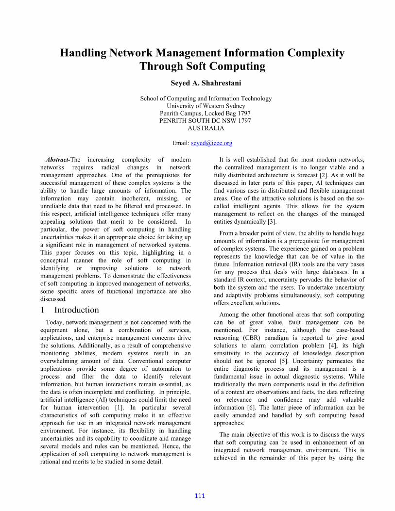
Handling Network Management Information ComplexityThrough Soft Computing

Seyed A. Shahrestani

School of Computing and Information TechnologyUniversity of Western Sydney

Penrith Campus, Locked Bag 1797 PENRITH SOUTH DC NSW 1797

AUSTRALIA

Email: seyed@ieee.org

Abstract-The increasing complexity of modernnetworks requires radical changes in networkmanagement approaches. One of the prerequisites forsuccessful management of these complex systems is theability to handle large amounts of information. Theinformation may contain incoherent, missing, orunreliable data that need to be filtered and processed. Inthis respect, artificial intelligence techniques offer manyappealing solutions that merit to be considered. Inparticular, the power of soft computing in handlinguncertainties makes it an appropriate choice for taking upa significant role in management of networked systems.This paper focuses on this topic, highlighting in aconceptual manner the role of soft computing inidentifying or improving solutions to networkmanagement problems. To demonstrate the effectivenessof soft computing in improved management of networks,some specific areas of functional importance are alsodiscussed.

1 IntroductionToday, network management is not concerned with the

equipment alone, but a combination of services,applications, and enterprise management concerns drivethe solutions. Additionally, as a result of comprehensivemonitoring abilities, modern systems result in anoverwhelming amount of data. Conventional computerapplications provide some degree of automation toprocess and filter the data to identify relevantinformation, but human interactions remain essential, asthe data is often incomplete and conflicting. In principle,artificial intelligence (AI) techniques could limit the needfor human intervention [1]. In particular severalcharacteristics of soft computing make it an effectiveapproach for use in an integrated network managementenvironment. For instance, its flexibility in handlinguncertainties and its capability to coordinate and manageseveral models and rules can be mentioned. Hence, theapplication of soft computing to network management isrational and merits to be studied in some detail.

It is well established that for most modern networks,the centralized management is no longer viable and afully distributed architecture is forecast [2]. As it will bediscussed in later parts of this paper, AI techniques canfind various uses in distributed and flexible managementareas. One of the attractive solutions is based on the so-called intelligent agents. This allows for the systemmanagement to reflect on the changes of the managedentities dynamically [3].

From a broader point of view, the ability to handle hugeamounts of information is a prerequisite for managementof complex systems. The experience gained on a problemrepresents the knowledge that can be of value in thefuture. Information retrieval (IR) tools are the very basesfor any process that deals with large databases. In astandard IR context, uncertainty pervades the behavior ofboth the system and the users. To undertake uncertaintyand adaptivity problems simultaneously, soft computingoffers excellent solutions.

Among the other functional areas that soft computingcan be of great value, fault management can bementioned. For instance, although the case-basedreasoning (CBR) paradigm is reported to give goodsolutions to alarm correlation problem [4], its highsensitivity to the accuracy of knowledge descriptionshould not be ignored [5]. Uncertainty permeates theentire diagnostic process and its management is afundamental issue in actual diagnostic systems. Whiletraditionally the main components used in the definitionof a context are observations and facts, the data reflectingon relevance and confidence may add valuableinformation [6]. The latter piece of information can beeasily amended and handled by soft computing basedapproaches.

The main objective of this work is to discuss the waysthat soft computing can be used in enhancement of anintegrated network management environment. This isachieved in the remainder of this paper by using the

following structure. Section 2 presents the integratednetwork management environment, highlighting why AIand in particular fuzzy logic should be considered.Section 3 gives a brief review of soft computing. Notingthat soft computing can also be used to improve mostother AI approaches applied to network managementproblems, a very brief overview of some other AItechniques is also given. Section 4, focuses on specificapplications of soft computing in network management.The concluding remarks are given in Section 5.

2 Integrated Network ManagementThe need for distribution of network management is

already well established. This is evident by theapproaches such as definitions of remote monitoring(RMON) management information base (MIB) or mid-level manager MIB, for example. In general, theintegrated network management is concerned with acombination of issues relating to equipment, services,applications, and enterprise management. In this contextvarious new requirements need to be met by networkmanagement solutions. Some of these requirements arementioned in this section, while some possible enablingapproaches for complying with them are discussed inlater parts.

Help desk systems are designed to provide customersupport through a range of different technology andInformation Retrieval (IR) tools play a fundamental rolein this activity. Efficiency and effectiveness in dataretrieval being crucial for the overall problem solutionprocess heavily depend on the abstraction models. Theabstraction associated with an object should capture all itspeculiarities in an easily manageable representation.Identification of relevant features of achieving an objectabstraction is a complex task and presence ofuncertainties makes this task even harder [7].

For diagnosis purposes, focusing on case-basedreasoning (CBR) paradigm, models that capture therelevance and uncertainty of information in a dynamicmanner are essential. This is a requirement for modelsused in both diagnostic knowledge and processes. Basedon such models a conversational CBR shell implementingnearest-neighbor (NN) retrieval mechanisms for examplecan then be utilized to achieve high precision case-retrieval [6].

Distributed applications are evolving towardscompositions of modular software components with userinterfaces based on web browsers. Each of thesecomponents provides well-defined services that interactwith other components via network. The increase in thecomplexity of distribution makes it more difficult to

manage the end-to-end Quality-of-Service (QoS). Amanagement system deployed to diagnose QoS de-gradation should address two major issues. First, tomeasure the performance of applications, it needs a low-overhead, scalable system for measuring softwarecomponents. Second, the performance managementsystem must monitor selected measurements, diagnoseQoS degradation, adapt to the environment and integratewith network management systems [8].

3 Soft Computing and ArtificialIntelligence

Although the focus of this work is on applications ofsoft computing in network management, it can be notedthat soft computing can be used to improve most other AIapproaches, e.g. knowledge presentation in expertsystems. Therefore, this section gives a very briefoverview of soft computing and some other AIapproaches that are found to be of value in networkmanagement.

3.1 Soft ComputingThe subject of fuzzy logic is the representation of

imprecise descriptions and uncertainties in a logicalmanner. Many artificial intelligence based systems aremainly dependent on knowledge bases or input/outputdescriptions of the operation, rather than on deterministicmodels. Inadequacies in the knowledge base,insufficiency or unreliability of data on the particularobject under consideration, or stochastic relationsbetween propositions may lead to uncertainty. In expertsystems, lack of consensus among experts can also beconsidered as uncertainty. Also, humans (operators,experts…) prefer to think and reason qualitatively, whichleads to imprecise descriptions, models, and requiredactions. Zadeh introduced the calculus of fuzzy logic as ameans for representing imprecise propositions (in anatural language) as non-crisp, fuzzy constraints on avariable [9].

A fuzzy system must accept crisp inputs (e.g.measurements) and produce crisp outputs (e.g. controlactions), while fuzzy logical operations are used(internally) to reach fuzzy inferences. The representationof real valued (crisp) inputs as fuzzy sets is referred to asfuzzification and is closely related to the concept ofMembership Function (MF). A membership function is anumerical representation of the belief about the degreethat a fuzzy variable belongs to a fuzzy set A.

After applying the logical operations, the antecedentof each rule can be considered to have been satisfied to

some degree, referred to as the firing strength (see nextsection). The firing strength is a single number that willalso be used to shape the consequent of the rule, theoutput fuzzy set. This is done by considering theconsequent of a rule being true to the same degree ofmembership as its antecedent. The above implicationprocess is applied to all rules, and all the fuzzy sets thatrepresent the output of each rule are aggregated to form asingle fuzzy set. The defuzzification process maps theresulting (output) fuzzy set into a crisp output.

3.2 Knowledge Based and Expert SystemKnowledge Based Systems (KBS) are modular

structures in which the knowledge is separate from theinference procedure. Knowledge may be utilized in manyforms, e.g. collection of facts, heuristics, common sense,etc. In many cases, knowledge is represented byproduction rules or specification of the conditions thatmust be satisfied for the rule to become applicable. Alsoincluded are the provisions of what should be done incase a rule is activated. Production rules are IF--THENstatements; a ‘conclusion’ is arrived at, upon theestablishment of validity of a ‘premise’ or a number ofpremises [10]. Rule-based systems are popular in AIbecause rules are easy to understand and readily testable.

3.3 Artificial Neural NetworksArtificial Neural Networks (ANNs) are dense parallel

layers of simple computational nodes. The strengths ofthe links between the nodes are defined as connectionweights. In most cases, one input layer, one output layer,and two internal (hidden) layers will be consideredadequate to solve most problems [11]. This is consideredas a Multi-Layer Perceptron (MLP) and is widelypopular. The connection weights are usually adaptedduring the training period by back-propagation of errors,which results in a feed-forward network.

3.4 Pattern RecognitionPattern recognition is the ability to perceive structure in

some data; it is one of the aspects common to all AImethods. The raw input data is pre-processed to form apattern. A pattern is an extract of information regardingvarious characteristics or features of an object, state of asystem, etc. Patterns either implicitly or explicitly containnames and values of features, and if they exist,relationships among features. The entire act ofrecognition can be carried out in two steps. In the firststep a particular manifestation of an object is described in

terms of suitably selected features. The second step,which is much easier than the first one, is to define andimplement an unambiguous mapping of these featuresinto class--membership space [11].

Patterns whose feature values are real numbers can beviewed as vectors in n-dimensional space, where n is thenumber of features in each pattern. With thisrepresentation, each pattern corresponds to a point in then-dimensional metric feature space. In such a space,distance between two points indicates similarities (ordifferences) of the corresponding two patterns.Partitioning the feature space by any of the manyavailable methods then achieves the actual act ofclassification.

3.5 Case-based ReasoningCase-based reasoning (CBR) paradigm [12] starts from

the assumption that cognitive process is structured as acycle. The first step is to gather some knowledge, then theknowledge is used to solve a problem and, depending onthe result, one may decide to keep track of the newexperience. Experience is accumulated either by addingnew information or by adapting the existing knowledge.The idea is to solve a problem with the existing skills and,at the same time, improving these skills for future use.From the actual implementation point of view, the focusis on how to aggregate and store the information (cases)and how to retrieve them. The solution of a problemdepends on the ability of the system to retrieve similarcases for which a solution is already known. The morecommon retrieval techniques are inductive retrieval andnearest neighbor [6].

4 Network Management and SoftComputing

Several characteristics of soft computing make it aneffective approach for use in an integrated networkmanagement environment. In particular its flexibility inhandling uncertainties and its capability to manageseveral models and rules are of great value. We start thissection by giving a broad view of integrated networkmanagement tasks that soft computing is suitable for. Wethen proceed to discussing some specific applicationareas.

4.1 Classification of Tasks in ManagementLayers

Consider the hierarchical model for networkmanagement shown in Table 1 [1]. At the highest layer

the problems can be associated with an overwhelmingamount of data. The AI techniques should process thedata and present only the relevant information by actingas a decision-support tool. At this layer, the response timeis important but not critical. This type of task is wellsuited for techniques that implement search techniques,e.g. genetic algorithm. Also, model-based expert systemscan be used to hide the network complexity behindseveral abstraction levels. In this context soft computingcan be used to handle model/data uncertainties andambiguities while interpolating between (possibly)several emerging models. The resultant aggregate modelwill also have some degree of confidence attached to itthat will assist the operators in dealing with the presentedinformation.

LayerTasks/

RequirementsInformationFlow

ControlFlow

Business Decision

Support ↑ ↓

Service Information

Retrieval (IR) ↑ ↓

Network Resource

Management ↑ ↓

Element Fast Control(ConnectionAdmission) ↑ ↓

Table 1, Management layers (adapted from [1])

While in the next section we take a closer look at someof the tasks in the service layer, it can be noted that theabove discussion holds for both service and networkmanagement layers. For example, AI based networkmanagement systems that deal with the problems atnetwork layer, are mostly based upon expert systemtechniques [13]. At the elements management layerthough, the time response becomes the critical factor. Itmust be noted that fuzzy logic (and ANN)implementations can be hardware-based to achieve fastresponse (while most other AI approaches are software-based). At this layer, the environment changes rapidlyand a slow solution will become irrelevant. The availableinformation is often incomplete and incoherent [1]. Thefuzzy logic character in dealing with uncertainties alongwith its capabilities in handling several sources of

information (via interpolations and taking a supervisoryrole), make it an excellent choice for management supportat this layer.

4.2 Advanced Help Desk In a competitive business environment, customer

satisfaction is a vital objective for many companies: high-quality products and high-quality customer service aretwo strategic aspects. In this context, help desk systemsplay an important role providing customer support andfunctions like change, configuration and assetmanagement. The two main components of a help desksystem are the front-end and the back-end ones: theformer manages the interaction with customers while thelatter deals with information retrieval (IR) issues.

The IR process is based on matching of the objectdescriptions (system knowledge) with an ideal descriptionderived from the user query, while allowing for theexpression of different views on the same component. Itcan be noted that various elements may affect thecomputation of the relevance of a keyword for thedescription of an object [5]. Using soft computingenforces the possibility to express such elements througha complete relevance distribution (through membershipfunctions) that can be employed in the retrieval process.

The core functionality is the retrieval of data from adatabase whose abstraction matches the description of anideal object, inferred from a query. Implementation issuesare critical both for the overall performance of the systemand the accuracy of the retrieved information. Customersusually provide data with different degrees of confidencedepending on how that information has been collected.Current IR tools do not explicitly model the uncertaintyassociated with information but they mix the measure ofrelevance associated to information with the relativemeasure of confidence. They don’t even manage thefeedback provided by users about the accuracy andusefulness of the retrieved solutions. An effective use ofthat information is the key to enable a process of systemadaptation. The explicit management of relevance andconfidence on information, integrated with an adaptivityprocess is the key factor for improving the retrievalprecision of a help desk system [7].

Soft computing can be used to form an integratedapproach to both uncertainty and adaptivity problems.Keywords are still at the base of the abstraction model,but together with relevance information, they will beenriched with information on confidence degreeimplemented through the use of membership functions.

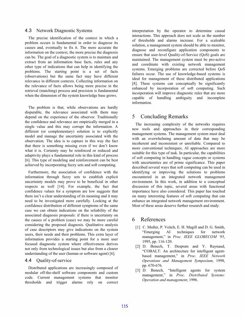
4.3 Network Diagnostic SystemsThe precise identification of the context in which a

problem occurs is fundamental in order to diagnose itscauses and, eventually to fix it. The more accurate theinformation on the context, the more precise the diagnosiscan be. The goal of a diagnostic system is to maintain andextract from an information base facts, rules and anyother type of indications that can help in identifying theproblems. The starting point is a set of facts(observations) but the same fact may have differentrelevance in different contexts. Collecting information onthe relevance of facts allows being more precise in theretrieval (matching) process and precision is fundamentalwhen the dimension of the system knowledge base grows.

The problem is that, while observations are hardlydisputable, the relevance associated with them maydepend on the experience of the observer. Traditionallythe confidence and relevance are empirically merged in asingle value and this may corrupt the information. Adifferent (or complementary) solution is to explicitlymodel and manage the uncertainty associated with theobservation. The idea is to capture in this way the factthat there is something missing even if we don’t knowwhat it is. Certainty may be reinforced or reduced andadaptivity plays a fundamental role in this kind of process[6]. This type of modeling and reinforcement can be bestachieved by incorporating fuzzy sets and soft computing.

Furthermore, the association of confidence with theinformation through fuzzy sets to establish explicituncertainty models may prove to be beneficial in otherrespects as well [14]. For example, the fact thatconfidence values for a symptom are low suggests thatthere isn’t a clear understanding of its meaning and it mayneed to be investigated more carefully. Looking at theconfidence distribution of different symptoms of the samecase we can obtain indications on the reliability of theassociated diagnosis proposals: if there is uncertainty onthe causes of a problem (case) we may be more carefulconsidering the proposed diagnosis. Qualitative analysisof case descriptors may give indications on the systemusers, their needs and their problems. This extra layer ofinformation provides a starting point for a more userfocused diagnostic system where effectiveness derivesnot only from technological issues but also from a clearerunderstanding of the user (human or software agent) [6].

4.4 Quality-of-serviceDistributed applications are increasingly composed of

modular off-the-shelf software components and customcode. Current management systems that monitorthresholds and trigger alarms rely on correct

interpretation by the operator to determine causalinteractions. This approach does not scale as the numberof thresholds and alarms increase. For a scaleablesolution, a management system should be able to monitor,diagnose and reconfigure application components toensure that user-level Quality-of-Service (QoS) goals aremaintained. The management system must be pro-activeand coordinate with existing network managementsystems. Emerging problems are corrected before QoSfailures occur. The use of knowledge-based systems isideal for management of these distributed applications[8]. These systems can conceptually be significantlyenhanced by incorporation of soft computing. Suchincorporation will improve diagnostic rules that are morecapable of handling ambiguity and incompleteinformation.

5 Concluding RemarksThe increasing complexity of the networks requires

new tools and approaches in their correspondingmanagement systems. The management system must dealwith an overwhelming amount of data that may beincoherent and inconsistent or unreliable. Compared tomore conventional techniques, AI approaches are moresuitable for this type of task. In particular, the capabilitiesof soft computing in handling vague concepts or systemswith uncertainties are of prime significance. This paperdescribed several ways that soft computing can be used inidentifying or improving the solutions to problemsencountered in an integrated network managementenvironment. In this work, in addition to a conceptualdiscussion of this topic, several areas with functionalimportance have also considered. This paper has touchedon many interesting features of soft computing that canenhance an integrated network management environment.Most of these areas deserve further research and study.

6 References[1] C. Muller, P. Veitch, E. H. Magill and D. G. Smith,

“Emerging AI techniques for networkmanagement,” in Proc. IEEE GLOBECOM ’95,1995, pp. 116-120.

[2] D. Benech, T. Desprats and Y. Raynaud,“COBALT: An architecture for intelligent agent-based management,” in Proc. IEEE NetworkOperations and Management Symposium, 1998,pp. 670-676.

[3] D. Benech, “Intelligent agents for systemmanagement,” in Proc. Distributed Systems:Operation and management, 1996.

[4] L. Lewis and P. Kaikini, “An approach to thealarm correlation problem using inductivemodeling technology,” Technical Note ctron-lml-93-03, Cabletron Systems R&D Center,Merrimack, 1993.

[5] G. Piccinelli and M. C. Mont, “Uncertaintymodelling for adaptive information management,”Technical Report HPL-98-86, HP Laboratories,Bristol, 1998. Available athttp://www.hpl.hp.com/techreports/98/HPL-98-86.html

[6] G. Piccinelli, “Uncertainty modelling in diagnosticsystems: An adaptive solution,” Technical ReportHPL-98-37, HP Laboratories, Bristol, 1998.Available athttp://www.hpl.hp.com/techreports/98/HPL-98-37.html

[7] G. Piccinelli and M. C. Mont, “Fuzzy-set basedinformation retrieval for advanced help desk,”Technical Report HPL-98-65, HP Laboratories,Bristol, 1998. Available athttp://www.hpl.hp.com/techreports/98/HPL-98-65.html

[8] J. Martinka, J. Pruyne and M. Jain “Quality-of-service measurements with model-basedmanagement for networked applications,”Technical Report HPL-97-167, HP Laboratories,Palo Alto, 1998. Available athttp://www.hpl.hp.com/techreports/97/HPL-97-167R1.html

[9] L. A. Zadeh, “Fuzzy sets,” Information andControl, vol. 8, pp. 338-353, 1965.

[10] S. A. Shahrestani, H. Yee, and J. Ypsilantis,“Adaptive recognition by specialized grouping ofclasses,” in Proc. 4th IEEE Conference on ControlApplications, Albany, New York, 1995, pp. 637-642.

[11] Y. H. Pao, Adaptive Pattern Recognition andNeural Networks. Addison Wesley, USA, 1989.

[12] K.D. Althoff and S. Wess, “Case-based reasoningand expert system development,” in ContemporaryKnowledge Engineering and Cognition, Springer-Verlag, USA, 1991.

[13] N. Nuansri, T. S. Dillon and S. Singh, “Anapplication of neural network and rule-basedsystem for network management,” in Proc. 30th

Hawaii International Conference on SystemSciences, 1997, pp. 474-483.

[14] L. A. Zadeh, “The role of fuzzy logic in themanagement of uncertainty in expert systems,'”Fuzzy Sets and Systems, vol. 11, pp. 199-228, 1983.

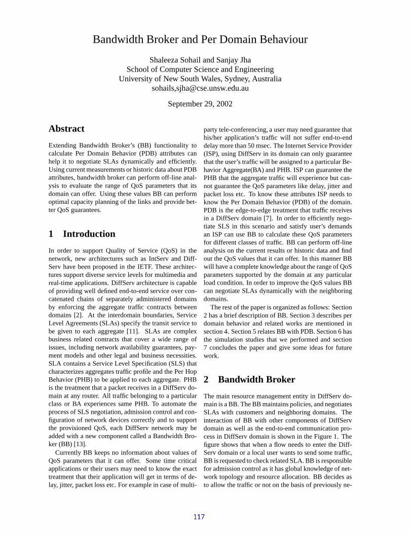
Bandwidth Broker and Per Domain Behaviour

Shaleeza Sohail and Sanjay JhaSchool of Computer Science and Engineering

University of New South Wales, Sydney, Australiasohails,sjha@cse.unsw.edu.au

September 29, 2002

Abstract

Extending Bandwidth Broker’s (BB) functionality tocalculate Per Domain Behavior (PDB) attributes canhelp it to negotiate SLAs dynamically and efficiently.Using current measurements or historic data about PDBattributes, bandwidth broker can perform off-line anal-ysis to evaluate the range of QoS parameters that itsdomain can offer. Using these values BB can performoptimal capacity planning of the links and provide bet-ter QoS guarantees.

1 Introduction

In order to support Quality of Service (QoS) in thenetwork, new architectures such as IntServ and Diff-Serv have been proposed in the IETF. These architec-tures support diverse service levels for multimedia andreal-time applications. DiffServ architecture is capableof providing well defined end-to-end service over con-catenated chains of separately administered domainsby enforcing the aggregate traffic contracts betweendomains [2]. At the interdomain boundaries, ServiceLevel Agreements (SLAs) specify the transit service tobe given to each aggregate [11]. SLAs are complexbusiness related contracts that cover a wide range ofissues, including network availability guarantees, pay-ment models and other legal and business necessities.SLA contains a Service Level Specification (SLS) thatcharacterizes aggregates traffic profile and the Per HopBehavior (PHB) to be applied to each aggregate. PHBis the treatment that a packet receives in a DiffServ do-main at any router. All traffic belonging to a particularclass or BA experiences same PHB. To automate theprocess of SLS negotiation, admission control and con-figuration of network devices correctly and to supportthe provisioned QoS, each DiffServ network may beadded with a new component called a Bandwidth Bro-ker (BB) [13].

Currently BB keeps no information about values ofQoS parameters that it can offer. Some time criticalapplications or their users may need to know the exacttreatment that their application will get in terms of de-lay, jitter, packet loss etc. For example in case of multi-

party tele-conferencing, a user may need guarantee thathis/her application’s traffic will not suffer end-to-enddelay more than 50 msec. The Internet Service Provider(ISP), using DiffServ in its domain can only guaranteethat the user’s traffic will be assigned to a particular Be-havior Aggregate(BA) and PHB. ISP can guarantee thePHB that the aggregate traffic will experience but can-not guarantee the QoS parameters like delay, jitter andpacket loss etc. To know these attributes ISP needs toknow the Per Domain Behavior (PDB) of the domain.PDB is the edge-to-edge treatment that traffic receivesin a DiffServ domain [7]. In order to efficiently nego-tiate SLS in this scenario and satisfy user’s demandsan ISP can use BB to calculate these QoS parametersfor different classes of traffic. BB can perform off-lineanalysis on the current results or historic data and findout the QoS values that it can offer. In this manner BBwill have a complete knowledge about the range of QoSparameters supported by the domain at any particularload condition. In order to improve the QoS values BBcan negotiate SLAs dynamically with the neighboringdomains.

The rest of the paper is organized as follows: Section2 has a brief description of BB. Section 3 describes perdomain behavior and related works are mentioned insection 4. Section 5 relates BB with PDB. Section 6 hasthe simulation studies that we performed and section7 concludes the paper and give some ideas for futurework.

2 Bandwidth Broker

The main resource management entity in DiffServ do-main is a BB. The BB maintains policies, and negotiatesSLAs with customers and neighboring domains. Theinteraction of BB with other components of DiffServdomain as well as the end-to-end communication pro-cess in DiffServ domain is shown in the Figure 1. Thefigure shows that when a flow needs to enter the Diff-Serv domain or a local user wants to send some traffic,BB is requested to check related SLA. BB is responsiblefor admission control as it has global knowledge of net-work topology and resource allocation. BB decides asto allow the traffic or not on the basis of previously ne-

1

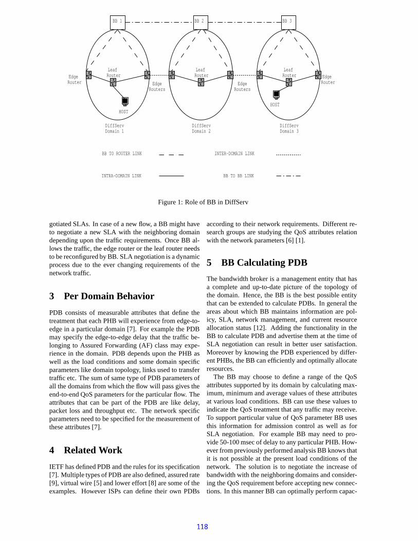
BB 2 BB 1 BB 3

DiffServ Domain 1

DiffServDomain 2

DiffServ Domain 3

Edge Router Edge

Routers

Leaf Router

Host

Edge Router Edge

Routers

Leaf Router

Leaf Router

BB TO ROUTER LINK INTER-DOMAIN LINK

INTRA-DOMAIN LINK BB TO BB LINK

HOSTHOST

Figure 1: Role of BB in DiffServ

gotiated SLAs. In case of a new flow, a BB might haveto negotiate a new SLA with the neighboring domaindepending upon the traffic requirements. Once BB al-lows the traffic, the edge router or the leaf router needsto be reconfigured by BB. SLA negotiation is a dynamicprocess due to the ever changing requirements of thenetwork traffic.

3 Per Domain Behavior

PDB consists of measurable attributes that define thetreatment that each PHB will experience from edge-to-edge in a particular domain [7]. For example the PDBmay specify the edge-to-edge delay that the traffic be-longing to Assured Forwarding (AF) class may expe-rience in the domain. PDB depends upon the PHB aswell as the load conditions and some domain specificparameters like domain topology, links used to transfertraffic etc. The sum of same type of PDB parameters ofall the domains from which the flow will pass gives theend-to-end QoS parameters for the particular flow. Theattributes that can be part of the PDB are like delay,packet loss and throughput etc. The network specificparameters need to be specified for the measurement ofthese attributes [7].

4 Related Work

IETF has defined PDB and the rules for its specification[7]. Multiple types of PDB are also defined, assured rate[9], virtual wire [5] and lower effort [8] are some of theexamples. However ISPs can define their own PDBs

according to their network requirements. Different re-search groups are studying the QoS attributes relationwith the network parameters [6] [1].

5 BB Calculating PDB

The bandwidth broker is a management entity that hasa complete and up-to-date picture of the topology ofthe domain. Hence, the BB is the best possible entitythat can be extended to calculate PDBs. In general theareas about which BB maintains information are pol-icy, SLA, network management, and current resourceallocation status [12]. Adding the functionality in theBB to calculate PDB and advertise them at the time ofSLA negotiation can result in better user satisfaction.Moreover by knowing the PDB experienced by differ-ent PHBs, the BB can efficiently and optimally allocateresources.

The BB may choose to define a range of the QoSattributes supported by its domain by calculating max-imum, minimum and average values of these attributesat various load conditions. BB can use these values toindicate the QoS treatment that any traffic may receive.To support particular value of QoS parameter BB usesthis information for admission control as well as forSLA negotiation. For example BB may need to pro-vide 50-100 msec of delay to any particular PHB. How-ever from previously performed analysis BB knows thatit is not possible at the present load conditions of thenetwork. The solution is to negotiate the increase ofbandwidth with the neighboring domains and consider-ing the QoS requirement before accepting new connec-tions. In this manner BB can optimally perform capac-

50 VoIP Soources & Sinks Pair

BE Source & Sink pair

50 WebClients

Bottleneck LinkVariable Bandwidth

10 ms Delay2.0---3.0 Mbps

Router1 Router2

Web Server 1

Web Server 2

Web Server 3Web Server 4Web Server 5BE Source & Sink Pair

50 VoIP Sources & Sinks pairs

All Access Links have 10 Mbps bandwidth and 0.1 ms delay

Figure 2: Topology

ity planning of the links of the domain.The simulation study in the next section calculates

different values for some QoS attributes by changingfew parameters. This simulation study shows that byusing simple mechanism a BB can be extended to mon-itor different attributes of PDB.

6 Simulations

The simulations are performed using the Network Sim-ulator (NS) [10]. Some of the simulation parameters aretaken from the simulation study of DiffServ [1], how-ever the scheduler used is weighted fair queuing [14]. Inthe simulation, the sources are generating traffic at con-stant rate and the bandwidth of the link changes for eachsimulation run. The values of QoS parameters changewith the change of link capacity and the minimum linkcapacity can be found in this way that can support someparticular QoS value. The impact of capacity on the at-tributes can help BB to decide what link capacity to useto transfer traffic, if certain QoS requirements like de-lay, packet loss etc; at a particular load condition, are tobe fulfilled.

6.1 Simulation Topology and Parameters

The network is a simple dumb bell shape as shown inFigure 2. There is one bottle-neck link which has vary-ing bandwidth with 10 msec delay. On one side ofbottle-neck link there are 50 web clients and 50 voicesources/sinks. On the other side there are 5 web serversand 50 voice sources/sinks. There are two best effortsources and sinks to produce congestion on the bottle-neck link. There is minimum bandwidth reserved for

the BE sources but these sources always send at the ratehigher than the rate allocated to them.

Following three types of traffic are used in the net-work:

1. Voice traffic: The voice traffic is modeled as VoIPand there is no compression and silence suppres-sion [1]. There are 50 voice source/sink pairs ateach side of bottleneck link. The VoIP sources areactually UDP ON/OFF sources. The inter call gapis 15 minutes and the mean rate of traffic is 86.4Kbps. The 80% of the calls are short calls andrest are long calls. The On time for short callsis 3 minutes and that for long calls is 8 minutes.The VoIP traffic is assigned Expedited Forwarding(EF) PHB. EF PHB provides low latency, low loss,low jitter, assured bandwidth service through Diff-Serv domains [4].

2. Data Traffic: The data traffic is web traffic gen-erated by the request and reply interaction ofHTTP/1.1 between web servers and clients. Thereare 50 clients requesting to 5 web servers [1]. Thenumber of objects requested are random. Thistraffic is assigned to Assured Forwarding (AF)PHB. AF PHB provides forwarding assurance tothe packets belonging to this PHB [3].

3. Best Effort: The Best Effort (BE) traffic is a sim-ple UDP source generating at the rate higher thanthe rate it is allowed. The traffic assigned to BEPHB has no assurance from DiffServ domain.

6.2 Simulation Results

The end-to-end delay and packet loss for differentclasses are measured. These values vary with the

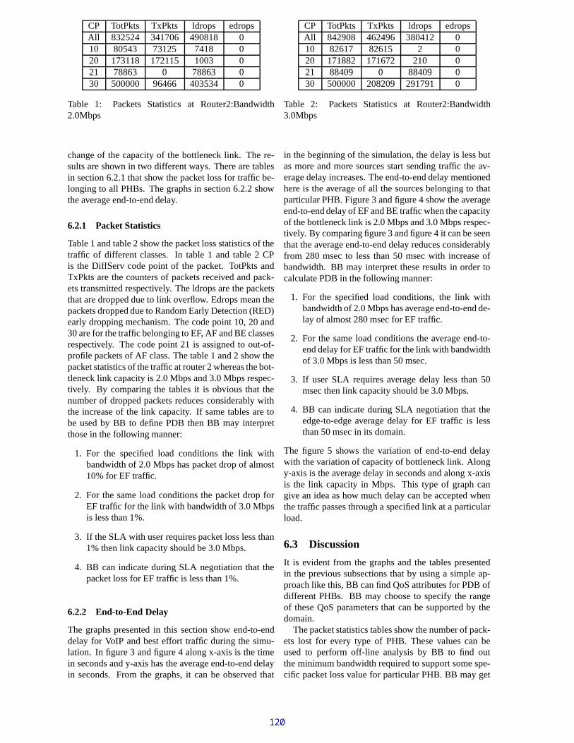
CP TotPkts TxPkts ldrops edropsAll 832524 341706 490818 010 80543 73125 7418 020 173118 172115 1003 021 78863 0 78863 030 500000 96466 403534 0

Table 1: Packets Statistics at Router2:Bandwidth2.0Mbps

change of the capacity of the bottleneck link. The re-sults are shown in two different ways. There are tablesin section 6.2.1 that show the packet loss for traffic be-longing to all PHBs. The graphs in section 6.2.2 showthe average end-to-end delay.

6.2.1 Packet Statistics

Table 1 and table 2 show the packet loss statistics of thetraffic of different classes. In table 1 and table 2 CPis the DiffServ code point of the packet. TotPkts andTxPkts are the counters of packets received and pack-ets transmitted respectively. The ldrops are the packetsthat are dropped due to link overflow. Edrops mean thepackets dropped due to Random Early Detection (RED)early dropping mechanism. The code point 10, 20 and30 are for the traffic belonging to EF, AF and BE classesrespectively. The code point 21 is assigned to out-of-profile packets of AF class. The table 1 and 2 show thepacket statistics of the traffic at router 2 whereas the bot-tleneck link capacity is 2.0 Mbps and 3.0 Mbps respec-tively. By comparing the tables it is obvious that thenumber of dropped packets reduces considerably withthe increase of the link capacity. If same tables are tobe used by BB to define PDB then BB may interpretthose in the following manner:

1. For the specified load conditions the link withbandwidth of 2.0 Mbps has packet drop of almost10% for EF traffic.

2. For the same load conditions the packet drop forEF traffic for the link with bandwidth of 3.0 Mbpsis less than 1%.

3. If the SLA with user requires packet loss less than1% then link capacity should be 3.0 Mbps.

4. BB can indicate during SLA negotiation that thepacket loss for EF traffic is less than 1%.

6.2.2 End-to-End Delay

The graphs presented in this section show end-to-enddelay for VoIP and best effort traffic during the simu-lation. In figure 3 and figure 4 along x-axis is the timein seconds and y-axis has the average end-to-end delayin seconds. From the graphs, it can be observed that

CP TotPkts TxPkts ldrops edropsAll 842908 462496 380412 010 82617 82615 2 020 171882 171672 210 021 88409 0 88409 030 500000 208209 291791 0

Table 2: Packets Statistics at Router2:Bandwidth3.0Mbps

in the beginning of the simulation, the delay is less butas more and more sources start sending traffic the av-erage delay increases. The end-to-end delay mentionedhere is the average of all the sources belonging to thatparticular PHB. Figure 3 and figure 4 show the averageend-to-end delay of EF and BE traffic when the capacityof the bottleneck link is 2.0 Mbps and 3.0 Mbps respec-tively. By comparing figure 3 and figure 4 it can be seenthat the average end-to-end delay reduces considerablyfrom 280 msec to less than 50 msec with increase ofbandwidth. BB may interpret these results in order tocalculate PDB in the following manner:

1. For the specified load conditions, the link withbandwidth of 2.0 Mbps has average end-to-end de-lay of almost 280 msec for EF traffic.

2. For the same load conditions the average end-to-end delay for EF traffic for the link with bandwidthof 3.0 Mbps is less than 50 msec.

3. If user SLA requires average delay less than 50msec then link capacity should be 3.0 Mbps.

4. BB can indicate during SLA negotiation that theedge-to-edge average delay for EF traffic is lessthan 50 msec in its domain.

The figure 5 shows the variation of end-to-end delaywith the variation of capacity of bottleneck link. Alongy-axis is the average delay in seconds and along x-axisis the link capacity in Mbps. This type of graph cangive an idea as how much delay can be accepted whenthe traffic passes through a specified link at a particularload.

6.3 Discussion

It is evident from the graphs and the tables presentedin the previous subsections that by using a simple ap-proach like this, BB can find QoS attributes for PDB ofdifferent PHBs. BB may choose to specify the rangeof these QoS parameters that can be supported by thedomain.

The packet statistics tables show the number of pack-ets lost for every type of PHB. These values can beused to perform off-line analysis by BB to find outthe minimum bandwidth required to support some spe-cific packet loss value for particular PHB. BB may get

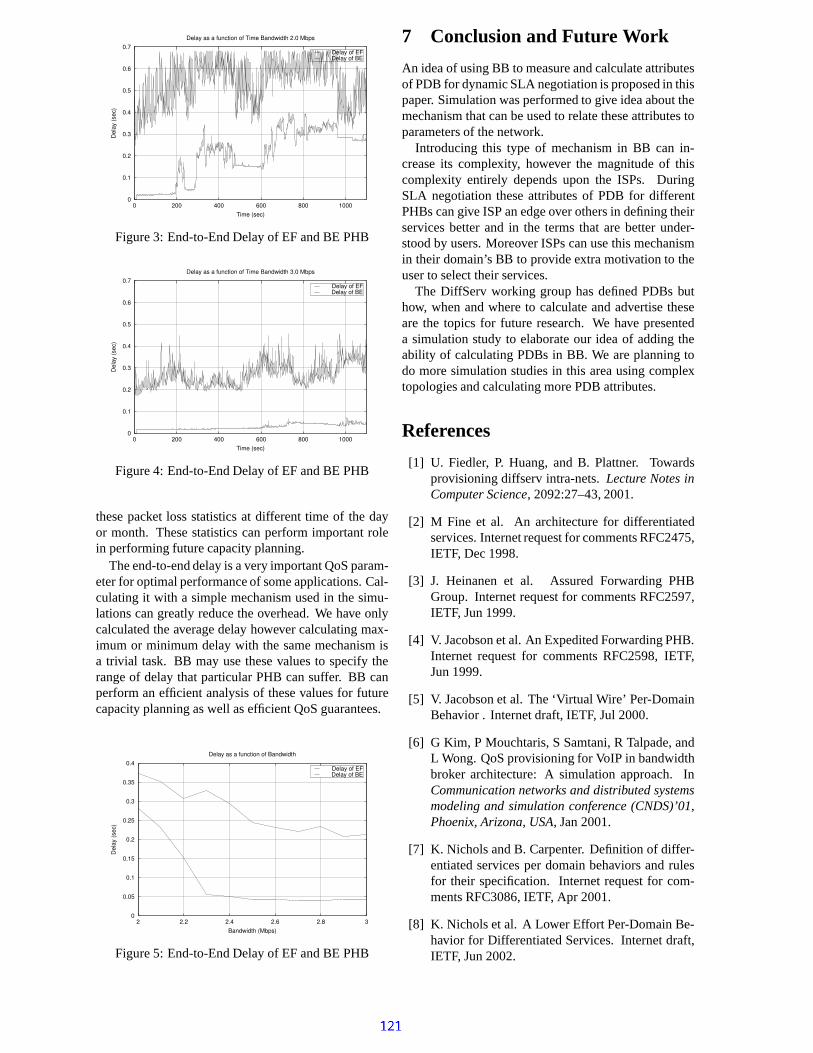
0

0.1

0.2

0.3

0.4

0.5

0.6

0.7

0 200 400 600 800 1000

Del

ay (s

ec)

Time (sec)

Delay as a function of Time Bandwidth 2.0 Mbps

Delay of EFDelay of BE

Figure 3: End-to-End Delay of EF and BE PHB

0

0.1

0.2

0.3

0.4

0.5

0.6

0.7

0 200 400 600 800 1000

Del

ay (s

ec)

Time (sec)

Delay as a function of Time Bandwidth 3.0 Mbps

Delay of EFDelay of BE

Figure 4: End-to-End Delay of EF and BE PHB

these packet loss statistics at different time of the dayor month. These statistics can perform important rolein performing future capacity planning.

The end-to-end delay is a very important QoS param-eter for optimal performance of some applications. Cal-culating it with a simple mechanism used in the simu-lations can greatly reduce the overhead. We have onlycalculated the average delay however calculating max-imum or minimum delay with the same mechanism isa trivial task. BB may use these values to specify therange of delay that particular PHB can suffer. BB canperform an efficient analysis of these values for futurecapacity planning as well as efficient QoS guarantees.

0

0.05

0.1

0.15

0.2

0.25

0.3

0.35

0.4

2 2.2 2.4 2.6 2.8 3

Del

ay (s

ec)

Bandwidth (Mbps)

Delay as a function of Bandwidth

Delay of EFDelay of BE

Figure 5: End-to-End Delay of EF and BE PHB

7 Conclusion and Future Work

An idea of using BB to measure and calculate attributesof PDB for dynamic SLA negotiation is proposed in thispaper. Simulation was performed to give idea about themechanism that can be used to relate these attributes toparameters of the network.

Introducing this type of mechanism in BB can in-crease its complexity, however the magnitude of thiscomplexity entirely depends upon the ISPs. DuringSLA negotiation these attributes of PDB for differentPHBs can give ISP an edge over others in defining theirservices better and in the terms that are better under-stood by users. Moreover ISPs can use this mechanismin their domain’s BB to provide extra motivation to theuser to select their services.

The DiffServ working group has defined PDBs buthow, when and where to calculate and advertise theseare the topics for future research. We have presenteda simulation study to elaborate our idea of adding theability of calculating PDBs in BB. We are planning todo more simulation studies in this area using complextopologies and calculating more PDB attributes.

References

[1] U. Fiedler, P. Huang, and B. Plattner. Towardsprovisioning diffserv intra-nets. Lecture Notes inComputer Science, 2092:27–43, 2001.

[2] M Fine et al. An architecture for differentiatedservices. Internet request for comments RFC2475,IETF, Dec 1998.

[3] J. Heinanen et al. Assured Forwarding PHBGroup. Internet request for comments RFC2597,IETF, Jun 1999.

[4] V. Jacobson et al. An Expedited Forwarding PHB.Internet request for comments RFC2598, IETF,Jun 1999.

[5] V. Jacobson et al. The ‘Virtual Wire’ Per-DomainBehavior . Internet draft, IETF, Jul 2000.

[6] G Kim, P Mouchtaris, S Samtani, R Talpade, andL Wong. QoS provisioning for VoIP in bandwidthbroker architecture: A simulation approach. InCommunication networks and distributed systemsmodeling and simulation conference (CNDS)’01,Phoenix, Arizona, USA, Jan 2001.

[7] K. Nichols and B. Carpenter. Definition of differ-entiated services per domain behaviors and rulesfor their specification. Internet request for com-ments RFC3086, IETF, Apr 2001.

[8] K. Nichols et al. A Lower Effort Per-Domain Be-havior for Differentiated Services. Internet draft,IETF, Jun 2002.

[9] N. Seddigh et al. An assured rate per-domain be-viour for differentiated services. Internet draft,IETF, Feb 2001.

[10] Network Simulator. NS-2. http://www.isi.edu/nsnam/ns/.

[11] S Sohail and S Jha. The survey of bandwidthbroker. Technical Report UNSW CSE TR 0206,School of Computer Science and Engineering,University of New South Wales, Sydney 2052Australia, May 2002.

[12] B. Teitelbaum and P. Chimento. Qbonebandwidth broker architecture. Work inProgress. at http://qbone.ctit.utwente.nl /de-liverables/1999/d2/bboutline2.htm, 1999.

[13] B. Teitelbaum and R. Geib. Internet2 QBone: ATest Bed for differentiated service. In INET’99,The Internet Global Summit, San Jose, CA, USA,Jun 1999.

[14] WFQ scheduler for. NS-2. http://www.tik.ee.ethz.ch/ fiedler/provisioning.html.

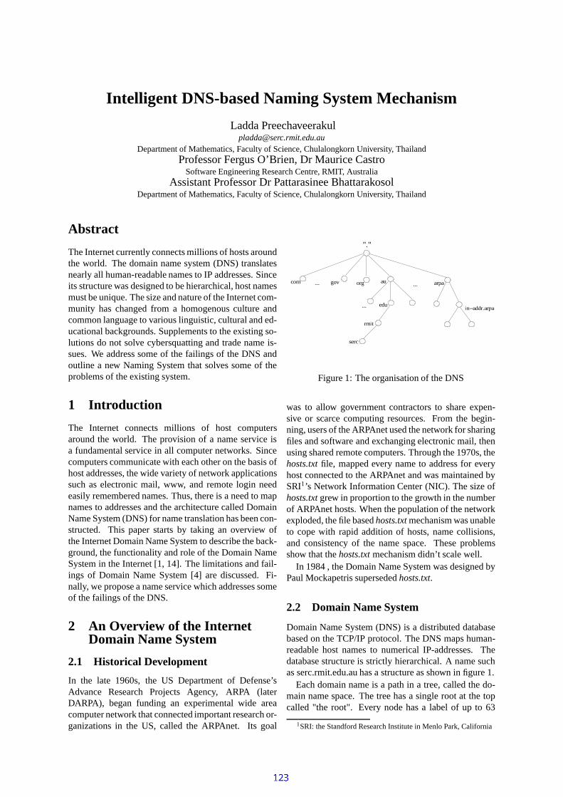
Intelligent DNS-based Naming System Mechanism

Ladda Preechaveerakulpladda@serc.rmit.edu.au

Department of Mathematics, Faculty of Science, Chulalongkorn University, ThailandProfessor Fergus O’Brien, Dr Maurice Castro

Software Engineering Research Centre, RMIT, AustraliaAssistant Professor Dr Pattarasinee Bhattarakosol

Department of Mathematics, Faculty of Science, Chulalongkorn University, Thailand

Abstract

The Internet currently connects millions of hosts aroundthe world. The domain name system (DNS) translatesnearly all human-readable names to IP addresses. Sinceits structure was designed to be hierarchical, host namesmust be unique. The size and nature of the Internet com-munity has changed from a homogenous culture andcommon language to various linguistic, cultural and ed-ucational backgrounds. Supplements to the existing so-lutions do not solve cybersquatting and trade name is-sues. We address some of the failings of the DNS andoutline a new Naming System that solves some of theproblems of the existing system.

1 Introduction

The Internet connects millions of host computersaround the world. The provision of a name service isa fundamental service in all computer networks. Sincecomputers communicate with each other on the basis ofhost addresses, the wide variety of network applicationssuch as electronic mail, www, and remote login needeasily remembered names. Thus, there is a need to mapnames to addresses and the architecture called DomainName System (DNS) for name translation has been con-structed. This paper starts by taking an overview ofthe Internet Domain Name System to describe the back-ground, the functionality and role of the Domain NameSystem in the Internet [1, 14]. The limitations and fail-ings of Domain Name System [4] are discussed. Fi-nally, we propose a name service which addresses someof the failings of the DNS.

2 An Overview of the InternetDomain Name System

2.1 Historical Development

In the late 1960s, the US Department of Defense’sAdvance Research Projects Agency, ARPA (laterDARPA), began funding an experimental wide areacomputer network that connected important research or-ganizations in the US, called the ARPAnet. Its goal

com

"."

gov org au

... edu com

rmit

serc

arpa ... ...

in−addr.arpa

Figure 1: The organisation of the DNS

was to allow government contractors to share expen-sive or scarce computing resources. From the begin-ning, users of the ARPAnet used the network for sharingfiles and software and exchanging electronic mail, thenusing shared remote computers. Through the 1970s, thehosts.txt file, mapped every name to address for everyhost connected to the ARPAnet and was maintained bySRI1’s Network Information Center (NIC). The size ofhosts.txt grew in proportion to the growth in the numberof ARPAnet hosts. When the population of the networkexploded, the file based hosts.txt mechanism was unableto cope with rapid addition of hosts, name collisions,and consistency of the name space. These problemsshow that the hosts.txt mechanism didn’t scale well.

In 1984 , the Domain Name System was designed byPaul Mockapetris superseded hosts.txt.

2.2 Domain Name System

Domain Name System (DNS) is a distributed databasebased on the TCP/IP protocol. The DNS maps human-readable host names to numerical IP-addresses. Thedatabase structure is strictly hierarchical. A name suchas serc.rmit.edu.au has a structure as shown in figure 1.

Each domain name is a path in a tree, called the do-main name space. The tree has a single root at the topcalled "the root". Every node has a label of up to 63

1SRI: the Standford Research Institute in Menlo Park, California

AA DD

CC

BB

resolver

query

query

query

query

answer answer

referral

referral

1

2

3

4

5

6

7 8

Figure 2: The Resolution Process

characters except the root and must have a unique do-main name. A domain name that ends with a periodis called an absolute domain name or a fully qualifieddomain name (FQDN) for example: serc.rmit.edu.au.

The existing domain name space is categorized into2 types of top-level domain (TLD): generic (gTLD) andgeographic or country-code (ccTLD). The informationabout the domain name space is stored in programscalled name servers.

Resolvers are library routines called by programs tolook up names. A resolver performs name resolution orasks a name server to do it by querying name serversto determine a mapping from a name to an address.Queries may be recursive, in which case the servermust return the resolution response into a result, or non-recursive, in which case the server returns only the in-formation it knows.

A generic resolution example is shown in figure 2with a brief explanation

1. Name server A receives a query from the resolver.

2. Name server A queries Name server B.

3. Name server B refers name server A to other nameservers, including C.

4. Name server A queries name server C.

5. Name server C refers name server A to other nameservers, including D.

6. Name server A queries name server D.

7. Name server D answers.

8. Name server A returns answer to resolver

3 Limitations and Failings of theDomain Name System

Since the DNS structure is hierarchical, each host map-ping to each IP address needs to be unique in the tree.

There are 3 groups of limitations and failings in theDNS: uniqueness, scalability and anonymity.

Uniqueness

Legal and social problems have occurred. Intellectualproperty has been disputed. In this case, if the domainnames chosen by a person seem related to the tradenames or a company, the person may not be able touse them at all. The bad faith registration of a domainname, called cybersquatting, also occurred. The pop-ular address space has been exhausted in a very shorttime. There are many products and companies that le-gitimately use the same name. There is no systematicway to guess the required domain name and there isno practical way for them to share a name. Althoughsearch engines can sometimes assist, they cannot solveevery query. The search engines do not cover the en-tire web. New, poorly referenced sites might as well notexist and not all search engines find all web pages.

Scalability

The size and nature of the Internet community haschanged. Originally, it consisted of people from similarcultural backgrounds and a single language (English)and has expanded to encompass various linguistic, cul-tural and educational backgrounds [6].

Anonymity

It is sometimes necessary to say things anonymously.Domain names are easily traced back to someone higherin the tree. Thus, it is essentially impossible to protecta domain name from retribution while simultaneouslyadvertising its existence to potential correspondents.

4 A Variety of Proposed ExistingSolutions

We can divide the existing solutions into 2 groups.Those that supplement the existing DNS service and al-ternate name services.

4.1 Supplementing the Existing DNSService

Several approaches have been made to supplement-ing DNS. First, the Internet Corporation for AssignedNames and Numbers (ICANN) had an agreement to in-troduce new gTLDs for supporting a wide variety ofuser groups [11]. Second, some companies such asName Space or Image Online Design have tried to re-configure either DNS servers or individual PCs to easilyaccess more TLDs [2]. A new approach called Real-Names has been proposed to help novice users avoidboth the DNS and search engines altogether. How-ever, none of these approaches resolve the underlyingof uniqueness and postpone scalability issue.

Methods such as the single-proxy method, OnionRouting Protocol [8], Crowds [10] and Hordes has beenconsidered to support the anonymity issue [12].

4.2 Alternate Name Services

Several other name servers have been developed. In1986, Lampson and his colleaques at the DEC SystemsResearch Center have designed a global name service(GNS) [7] for use in an internetwork which supports anaming database that may extend to include millions ofhost computers and eventually e-mail addressing for bil-lions of users. A naming database in GNS compose ofa tree of directories holding names and values. Each di-rectory is assigned an integer, which serves as a uniquedirectory identifier(DI). GNS successfully addresses theneed for scalability and reconfigurability with the ex-ception of the solution adopted for merging and movingdirectory trees [5]. For example, 2 previously seperateGNS services may be integrated with the introductionof a new root above the two existing roots. The well-known directory tables are used to store the previousdirectory identifiers and remap to the current real rootdirectory of the naming database. Whenever the realroot of the naming database changes, all GNS serversare informed of the new location of the real root. In alarge-scale network, reconfiguration may occur at anylevel. This makes this table grow rapidly, conflicts withthe scalability goal.

The Handle System was developed to be a persistentname service and allow secured name resolution and ad-ministration over the Internet [13]. Persistent name ser-vice means that the system allows name to persist overchanges of location, ownership, and other network stateconditions.

The Network Information Service Plus (NIS+) fromthe Sunsoft engineering team [9] and Novell DirectoryService (NDS) from Novell, Inc. [3] are being devel-oped their service not only to support in local area net-work but also supplement and compatability on the In-ternet. These systems are actively persuing the scalabil-ity, but are typically targeted within organisations.

Table 1 summarizes various naming system features.Furthermore, we conclude each name service and its

role and functionality in Table 2.With these proposed solutions, we found that it

couldn’t solve the failings of the existing DNS. Table3 summarize the features of the existing solutions

5 The New Proposal

We are proposing a name service which addresses someof the failing of DNS. We required that the server has:

1. Sharing names: the ability to share unique nameequitably among multiple valid claimants.

2. Scalability: it will remain effective when there is asignificant increase in the number of resources andthe number of users.

3. Decentralize administration via delegation: a do-main can divide into subdomain. Each subdomain

Figure 3: The organization of proposed DNS

or delegation is responsible for maintaining all thedata.

4. Efficiency: it is a distributed database with hier-archical structure that allows different parts of thenaming database to be maintain by different en-tities. Additionally, caching obviates the querywhich can’t answer locally and need to query otherservers.

5. Opacity: the use of a name conceals from the userlocation in IP-address components in a distributedsystem. Location opacity enables resources to beaccessed without requiring knowledge of their lo-cation.

6. Local customisation: partially specified names canuse sensible defaults based on user preferences andnetwork setup.

The new service employs both the concepts of sets andtrees to provide name to address translation. Each treecontains nodes which may refer to other servers or re-solve to a set of host IP addresses. A path through thetree terminates at a node. The set of host IP addressescontained in the node is returned as the result of thepath. The intersection of the sets from multiple pathsyields the name to address translation. For example, thepath marketA.vic.au.loc has a structure similar to theoriginal DNS structure. A resolvable domain name isa set of paths such as coke.tm:vic.au.loc:softdrink.prod.Its structure is shown in figure 3.

The dashed line represents the combination of do-main names to form a translation. To find the exactIP address, a new resolution mechanism has been con-structed. When a client queries name at a local nameserver, as shown in figure 4, and the local name serverdoes not know the answer, a process to divide the queryinto subqueries is invoked. Other name servers arequeried to determine a mapping from each subqueryname to a set of IP addresses. When each subquery re-turns, the process to intersect all subqueries is invokedand an answer is provided to the client. Figure 4 illus-trates the full resolution process with a brief explana-tion.

1. A client need to know the IP address of

Feature DNS GNS Handle System NIS+ NDS

Human-readable Yes Yes Yes Yes YesUnique Object Identifier (OID) No Yes Yes No No

Hierarchical name space Yes Yes Yes Yes YesLocation Transparent Yes Yes Yes Yes Yes

Support to Internet Yes Yes Yes No NoSupport to small network Yes Yes Yes Yes Yes

Support to large-scale network Yes Yes Yes Yes YesScalability Yes Yes/No2 Yes Yes YesSecurity Originally - No

Since 1987 - YesYes Yes Yes Yes

High Availability Yes Yes Yes Yes Yes

Table 1: Features of various naming system

Name Service Role and Functionality

Global Name Service (GNS) Support a large naming database distributed in an internetwork.Handle System A persistent name service for large number of entities and allow each

existing local name space join the global handle name space.NIS+ and NDS Services in each organization, stored information of any resources where

all workstations on network can access it.

Table 2: Name services and their role and functionality

Figure 4: The new resolution process

q :q :q :...:q , then it contacts the local nameserver A

2. Name server A takes each subquery (q , q , q , ...,q ) to name server B (root name server)

3. Name server B returns the root name server of eachsubquery to A

4. Name server A queries q to name server C

5. Each name server(C ) resolves its subquery byeither returning data held on the name server orquerying the set of name servers a delegation hasbeen made to. The server returns the union of thesets of IP-addresses found

6. Name server A intersects ans , ans , ..., ans

7. Name server A returns answer to resolver

6 Discussion

A hierarchical structure with a simple parent-child rela-tionships of the existing DNS provides a unique domainname. This restriction guarantees that a domain nameuniquely identifies a single leaf in the tree as shown infigure 1. Domain names at the leaves of the tree repre-sent individual hosts. An interior node of the tree canname both a host and point to information about the do-main. This structure limits the growth of the Internetcommunity.

The new structure, on the other hand, employs boththe concepts of sets and trees. Thus, domain namesat the leaves of the tree may not represent individualhosts but a set of host IP addresses. The flexibility ofthis structure reduces the problems of cybersquattingand trade names issues and still scales. The mechanismreduces cybersquatting and trademark problems by al-lowing many organisations to share a name - as is thecase with trademarks - which are distinguished by con-text. Cybersquatting is impractical when the monopolyenjoyed by a domain owner under the existing DNSis replaced by a system where names can be shared.

2not scalable in large-scale network when merging and movingdirectory tree

Sharing unique name Scalability Anonymity

Add new gTLD No No NoReconfigure DNS server or PCs No No No

RealNames Yes No NoProxy server or anonymous protocol No No Yes

Global Name Service (GNS) No Yes/No3 NoHandle System Yes No No

Network Information Service plus (NIS+) No No NoNovell Directory Service (NDS) No No No

Table 3: Features of the Existing Solutions

However, the intensiveness of the resolution process in-creases traffic. Caches maintained in the name serverswill be used to reduce the traffic.

7 Future Work

We are currently working on simulating the new system.Following that we will examine some problems with thesystem such as merging the huge sets associated withgeographical names and the handling of languages otherthan English.

Conclusion

The increasing demand for an Internet is affecting thepresent DNS used to map host names to IP addresses.The popular names are being exhausted by trademarkholders and cybersquatters. Different methods havebeen developed to supplement the existing DNS butthey do not solve the problems of intellectual property,cybersquatting, and name collisions. We propose a newname service that addresses some of the failings of DNSby remaining the uniqueness of name to address map-pings.

References

[1] P. Albitz and C. Liu. DNS and BIND. O’Reilly &Associates, third edition, 1998.

[2] A. Dornan. Can the internet move beyond dot-com? http://www.networkmagazine.com/article/nmg20010226s0008. March 2001.

[3] C. Andrew et al. E. Shropshire. Novell NDS De-veloper’s Guide. Novell Press, CA, 1999.

[4] L. Fonner. Fixing a flawed domain name system.Communications of the ACM, Volume 44, Num-ber 1, pages 19–21, January 2001.

3not scalable in large-scale network when merging and movingdirectory tree

[5] J. Dollimore G. Coulouris and T. Kindberg. Dis-tributed Systems Concepts and Design. Addison-Wesley Publishers Ltd., third edition, 2001.

[6] J. Horvath. What’s in a name?http://www.heise.de/tp/english/inhalt/te/5557.1.html.December 1999.

[7] B.W. Lampson and DEC Systems Research Cen-ter. Designing a global name service. In Proceed-ings 5th ACM Symposium on Principles of Dis-tributed Computing, pages 1–10, Calgary, Alberta,Canada, November 1986.

[8] P. Syverson M. Reed and D. Goldschlag. Proxiesfor anonymous routing. 12th Annual ComputerSecurity Applications Conference, IEEE, pages95–104, December 1995.

[9] R. Ramsey. All about administering NIS+. Moun-tain View, California : Sunsoft, second edition,1994.

[10] M.K. Reiter and A.D. Rubin. Crowds. ACMtransactions on Information and System Secu-rity(TISSEC), Volume 1, Number 1, pages 66–92,November 1998.

[11] Search Engine Report. Goodbye domain names,hello realnames? http://searchenginewatch.com/sereport/00/05-realnames.html. May 2000.

[12] C. Shields and B.N. Levine. A protocol for anony-mous communication over the internet. In Pro-ceeding 7th ACM conference on Computer andCommunication Security, pages 33–42, November2000.

[13] S.X. Sun and L. Lannon. Handle system overviewhttp://www.handle.net/overview-current.html.August 2001.

[14] W.R.Stevens. TCP/IP Illustrated, Volume 1 : TheProtocols. Addison-Wesley, 1994.

128

A NOVEL APPROACH TO REDUCE LATENCY FOR FR-ATM INTERWORKING

* H. Achi ** A. Rizk, ***A. Hellany

University of Western Sydney, School of Electrical Engineering & Industrial Design

Locked Bag 1797, Penrith South DC, NSW, Australia Phone: ** +61-2-47362-148, ***+61-2-47-360-126, Fax: +61-2-47-360-833

Email: *h.achi@uws.edu.au, **a.rizk@uws.edu.au, ***a.hellany@uws.edu.au,

ABSTRACT Asynchronous Transfer Mode (ATM) core networks constitute the backbone of many geographically spread Virtual Private Networks (VPN). The ever-increasing implementation of Frame Relay (FR) based VPNs over ATM backbone is leading to a considerable latency in customer services running over the network. This paper describes the process of build-up delay in FR ATM interworking. In addition, this paper proposes a new approach to reduce the latency by increasing the PIR/SIR ratio. Furthermore, A case study is introduced in order to validate the proposed method. Finally, the burstiness, virtual bandwidth and buffer overflow affecting the network performance are discussed. KEY WORDS Frame Relay (FR), Asynchronous Transfer Mode (ATM), Multi-Protocol Label Switching (MPLS), Partial Packet Discard (PPD), and Virtual Bandwidth. (VBW), Virtual Private Network (VPN).

1. INTRODUCTION Carriers and FR customers are generally concerned with several issues in implementing a FR service over ATM backbone. Customers generally connect to the ATM based VPN network using Frame Relay access. The switch interface terminating the customer access link performs a translation from Frame to ATM as per Frame Relay interworking Function standard FRF.8. This data is then delivered to the particular customer Core router ATM interface as shown in Figure 1. Frame Relay and ATM inherent certain characteristics, some of which tend to be problematic in FR-ATM interworking: • At the FR interface customers are able to burst

above the Frame Relay CIR and up to the Access Rate for extended periods. Frame Relay nodes use BECNs to signal the upstream device to throttle traffic when congestion occurs.

Figure 1: FR Service over ATM core based VPN network

ATM PIR/SIR/MBS= 143/116/210

ATM PIR/SIR/MBS=284/180/210

ATM Network

ATM S/W

ATM CoreRouter

CE1 CE2 ATM S/W

ATM S/W Circuit C1 FR CIR/BC/BE = 64/128/128 ATM PIR/SIR/MBS= 143/72/210

Circuit C2FR CIR/BC/BE =

128/256/256ATM PIR/SIR/MBS=

284/143/210

FR InterfaceNo Traffic Shaping

Access-rate = 256Kbps

FR Interface No Traffic Shaping Access-rate = 128Kbps

129

• ATM has no equivalence for BECNs [1] and thus cannot notify upstream devices to throttle back and enforces compliance to PCR, SCR and MBS parameters.

• Frame Relay and ATM specific terminology to describe the rate of user traffic: Access Rate (AR) and Committed Information Rate (CIR) are Frame Relay parameters, which describe the maximum allowed data rate, and the rate, which the network commits to deliver, respectively. Similarly the terms Peak Information Rate (PIR) and Sustained Information Rate (SIR) are the corresponding ATM parameters describing the maximum allowed data rate and the average data rate, which the network commits to deliver, respectively [2].

• The customer Frame Relay CIR is mapped to the equivalent ATM SIR (allowing for ATM overhead) and the Frame Access Rate is also mapped to the ATM PIR.

SLAs have been drafted to provide FR equivalent behavior when carrying it over ATM. However this expected behavior might not be totally met under this scenario for some inherent interworking limitations: • Inability to measure bursts above the Frame

CIR bandwidth. [3] This results from carriers using ATM interfaces in the ATM core routers. When ATM PVCs are loaded, the transfer rate will average to the ATM SCR bandwidth and consequently to the Frame CIR (not the access speed like Frame Relay).[5,6,7,8]

• Latency is increased to values higher than what the customer believes they should experience for their link size and traffic profile. [4] This is due to the longer than expected serialisation delay from the core router ATM interface. Under load data is clocked out of the interface at the SCR rate rather than the PCR rate (Frame Relay sends data at the access rate unless BECNs are received). [5,6,7,8]

In this paper we present a parameter configuration for FR-ATM interworking to reduce latency and obtain a FR network like behavior over ATM. This solution can be implemented in Virtual Private Networks using Frame relay. It may also be extended to include Multi-Protocol Label Switching (MPLS) VPN networks running over an ATM backbone when the impairing total roundtrip delay is reduced for packets sent across the various network hops. 2. DELAY CALCULATIONS. The End-to-End delay can be calculated as follows:

Let D (ab) be the delay experienced by the traffic sent from the branch FR Router to the Core ATM router, D (ab)= FR serialisation delay + ATM network delay + ATM switching delay (1) Let D (ba) be the delay experienced by the traffic sent from the ATM core router to the FR branch router, D (ba)= core router serialisation delay + network delay + switching delay + FR serialisation + FR queuing delay + FR buffer delay (2) Roundtrip delay = D (ab) + D (ba) (3) The roundtrip delay experienced by the data sent from a branch router to another branch router or back to itself.

Where FR serialisation delay = AR

FrameSize 8* (4)

Core router to ATM serialisation =

→

→

SIRat sent packetsfor 8*

PIRat sent packetsfor 8*

CIRFrameSize

ARFrameSize

(5)

• Switching delay =250 µ s/cell for CDVT of

250us. • Network delay = 5ms, it usually depends on the

number of hops and distances between the nodes.

• FR queuing delay = 5 ms, this depends on the switch fabric and packet processing.

• FR buffer delay depends on the amount of data held in the FR egress buffer when congestion occurs. The total delay of this buffer is equal the buffer threshold setting in ms. Under no congestion the buffer delay is nil.

The existing parameter settings, as shown in Figure 1, are: Access link = 128K, CIR=64K, PIR/SIR = 144/72 Kbps. It is assumed that the router can transmit at either AR or PIR. Hence,

D (ab)=128

8*1500 +5+0.25=99 ms

D (ba)= 128

8*1500 +5+.25+128

8*1500 +5+0=197.75ms

Worst case

D (ba)= 64

8*1500 +5+. 25+128

8*1500 +5+0=291.5 ms

130

Roundtrip delay is then 296.75 ms or at worst case = 390.5 ms. this round trip delay is large for certain applications and services which are delay sensitive. 3. PROPOSED SOLUTION To reduce the latency, we propose to increase the PIR to a larger value in order to decrease the serialisation from the core router to ATM interface. It is also possible to increase SIR to a value equivalent to the AR plus overheads as shown in Figure 2. However, there are several effects on the network, which need to be addressed and guarded against such as network burstiness, virtual bandwidth and buffer overflow. The proposed settings are provided in Table 1. The PVC specifications are listed below:

• FR service category: Low Delay • ATM service category: nrt-VBR • Interworking: service FRF.8 • ATM Traffic Policing: Tagging

• Frame Discard: Enabled Partial Packet Discard PPD

Under the proposed solution, the new delay becomes:

D (ab)=128

8*1500 +5+0.25=99 ms

D (ba)= 1024

8*1500 +5+.25+128

8*1500 +5+0=115.72ms

Worst case

D (ba)= 128

8*1500 +5+.25+128

8*1500 +5+0=197.75ms

Roundtrip delay is 214.72 ms or at worst case = 296.75 ms. this leads to a delay improvement of 24% to 41% in ATM-FR direction, whereas the Roundtrip delay improvement is 24% to27%.

Table 1. Summary table of parameter settings of the proposed solution.

ATM switch settings ATM Core Router settings

PIR =1145 kbps

( fixed to match 1024 Kbps FR access)

PIR=1145 kbps

SIR = 1.12625 * CIR kbps

(eg. for CIR = 64kbps, SIR= 72kbps)

SIR = 1.12625*FR Access Rate kbps

(eg. for AR=128kbps, SIR=143kbps)

MBS = 210 cells MBS=48 to144 cells

Figure 2: FR service over ATM core-based VPN network

ATM PIR/SIR/MBS= 1145/140/84

ATM PIR/SIR/MBS=1145/140/84

ATM Network

ATM S/W

ATM Core Router

CE1 CE2 ATM S/W

ATM S/W Circuit C1 FR CIR/BC/BE = 64/128/128 ATM PIR/SIR/MBS= 1145/72/210

Circuit C2FR CIR/BC/BE =

128/256/256ATM PIR/SIR/MBS=

1145/72/210

FR InterfaceNo Traffic Shaping

Access-rate = 256Kbps

FR Interface No Traffic Shaping Access-rate = 128Kbps

131

4. DISCUSSION The latency improvement in this proposed solution is attained with a tradeoff on network:

• The large PIR/SIR ratio (increased by 7 times) will increase the network burstiness allowing high bursts of traffic into the network and thus affecting the existing customer services. This effect can be countered by ensuring that the customer core ATM router is sending conforming traffic with low MBS and tagging any excess bursts.

• The network virtual bandwidth (VBW) will increase as a result of increasing PIR and SIR, thus reducing the number of possible connections to the network. This increase may be reflected as an additional cost to the customer’s PVC. However Maintaining the MBS at its default setting will factor for the increased bandwidth resources, so that no further bandwidth allocation is required.

• There is the possibility of overflowing the egress buffer at the FR interface, when the core ATM router sends non-conforming traffic ie flat lining at PIR or for large MBS. This will result in increasing the delays in the egress buffer. To guard against long buffer delays, the buffer threshold should be made small or at an optimised level depending on the frame size, PIR and MBS. The optimisation of the buffer setting requires further investigation.

• In order to guard against any adverse network congestion or service impact. Traffic policing should be ensured. Cells sent at PIR for longer than the recommended MBS will be tagged and dropped at the first sign of congestion. This option maximises the potential for concentrating tagged traffic – especially when employed in MPLS architecture. It relies on ATM switches policing and congestion control to tag and discard cells in the event of network congestion. It is expected that these surviving tagged cells will result in tagged Frames at the FR egress buffer, which will also be discarded upon this congesting (greater than Sever Congestion Threshold SCT setting).

• Early Packet Discard (EPD) or Partial Packet Discard (PPD) may also be implemented. EPD and PPD are congestion control mechanisms that are applied to AAL5 traffic, i.e. packet based traffic generated by data applications. These packets are often segmented into more than one ATM cell. Should congestion occur, one (or more) cell(s) pertaining to a packet may get discarded by the switch, resulting in a partially discarded packet that is carried to the destination but is indecipherable to the end application. PPD reduces this inefficiency by discarding all remaining cells in a partially

discarded packet. EPD takes this one step further by allowing all cells belonging to the packet that is being currently serviced to pass through, but discarding subsequent cells comprising one or more complete packets until the congestion is cleared. In the case of PPD, in order to maintain data flow between end-applications, cells containing the ‘End Of Packet’ indicator are not discarded.

5. CONCLUSION This paper identified the FR-ATM network latency, and proposed a solution to reduce the delays by increasing the PIR/SIR ratio. The impact of the novel approach on the network performance: burstiness, virtual bandwidth and buffer overflow is analysed and discussed. Series of strategies are proposed in order to guard against the stated impacts.

REFERENCES

[1] Sudhir Dixit and Stuart Elby “Frame Relay and ATM internetworking”, IEEE Communications Magazine, June 1996.

[2] Sudhir s. Dixit, Senior Member, IEEE, and Sharad Kumar “Traffic Descriptor Mapping and Traffic Control for Frame Relay Over ATM Network”, IEEE/ACM Transaction on Networking, VOL. 6, NO. 1, February 1998

[3] Jae-II Jung, “Translation of QoS parameters into ATM performance parameters in B-ISDN”, IEEE Communications Magazine, August 1996.

[4] J.W. Paek, S.W. Lee, C.H Oh and K.S Kim “A Study on traffic Parameters Estimation of call Admission Control in ATM Networks”, 1999 IEEE TELCON pages 836-839.

[5] “af-tm-0056.000, Traffic Management Specification”, The ATM Forum Technical Committee, version 4.0, April 1996

[6] “af-bici-0013.003, B-ICI Specification”, The ATM Forum Technical Committee, version 2.0, December 1995.

[7] “FRF.5, Frame Relay/ATM PVC Network Interworking Implementation Agreement”, The Frame Relay Forum, December 1994.

[8] “FRF.8, Frame Relay/ATM PVC Service Interworking Implementation Agreement”, The Frame Relay Forum, April 1995.

Web-Enabled Wireless Sensing

F. Naghdyi, Stephen Davisi, Gordon Wallaceii, Peter Innisii, iSchool of Electrical, Computer and Telecommunication Engineering

iiIntelligent Polymer Reseach Centre University of Wollongong, NSW, 2522, Australia

Abstract

A low cost framework is developed for a wireless web-enabled sensing device. The wireless communication is established through Bluetooth standards. A TINI (Tiny InterNet Interface) board developed by Dallas SemiConductors provides an optimal and very low cost but universal interface to the Internet. This represents the first stage of the work in developing a wireless embedded Internet control system. A review of the previous related work is carried out. An overview of the proposed system is provided and the design and development of each element of the system is explained. The results of the validation carried out on the system performance is presented and a critical analysis of the results is provided.

1. Introduction Distributed control has always been a superior method to centralised control. Design, implementation, troubleshooting and maintenance of a distributed system require much less effort and cost than when all the sensory information and control loops are processed by one central processor. The synchronization and integration of a distributed control requires the centralised collection of data. In addition, the operator interfaces to the distributed control system through a supervisory system to issue commands or vary the set points of the system. In such systems, sensors have traditionally been interfaced to the supervisory computer or the data-logging system through wires. The recent trends have been to interface the sensors and actuator through a network. There are also applications where expensive proprietary wireless communication protocols have been employed to transfer data or receive commands. This work explores how the latest advances in the Web-enabled devices and wireless communication can be employed to make sensing and control in distributed systems more flexible, efficient and cost effective. Web has traditionally been used to provide structured information and data as either static hypertext pages

or dynamic pages driven by a database. The concept of embedded Internet systems or web-enabled devices explores the possibility of providing real time data on Web, or driving a device via the Internet. In the study conducted in this project a low cost framework is developed for a wireless web-enabled sensing device. The wireless communication is established through Bluetooth standards. A TINI (Tiny InterNet Interface) board developed by Dallas SemiConductors provides an optimal and very low cost but universal interface to the Internet. This represents the first stage of the work in developing a wireless embedded Internet control system. While the methodology is kept as generic as possible, the work is focused on developing a device which is mounted on the knee sleeve of an Australian Football League player. The device provides information on whether the player has landed correctly after jumping. This helps to keep the player off the sidelines and to reduce the injuries. The motion of the knee is sensed by an intelligent polymer developed at Intelligent Polymer Research Centre, University of Wollongong. The knee motion is measured by a microcontroller and sent to a Bluetooth device for transmission to a second Bluetooth device. The signal is then passed to TINI and provided in real-time on the Web. In the course of the paper initially a review of the previous related work will be carried out. The focus will be on web-enabled devices and remote sensing using wireless radio. An overview of the proposed system will be then provided and the design and development of each element of the system will be explained. In the next part of the paper the results of the validation carried out on the system performance will be presented and a critical analysis of the results will be carried out.

2. Background The work reported in this project exploits two advances in computer technology and communication to produce a system that is highly flexible in its operation and function. They are short-range wireless radio and web-enabled devices. In this section a review of the previous work related to these two

fields will be studied as a background to highlight the significance and contribution of the work presented. Wireless sensing and actuation are far more attractive options to wired connections in an industrial or office environment. For example, wireless communication with a rotating or moving machine part is less challenging to implement than when wired. Wireless communication can also create new opportunities for more flexible manufacturing processes by establishing communication between a manufactured component and the production machine to activate the assembly or machining process needed by that component. The reliability and real-time performance of Bluetooth as a short-range radio system in an industrial environment, where electrical noise is prevalent has been an area of study and research. According to the study conducted by Blisrup and Wiberg [1] Bluetooth has potential to provide a wireless communication even in a very harsh industrial environment. There is, however, room to improve the applicability of the technology if additional error correction schemes and more adaptive error correction protocols are introduced. There are two different methods to accommodate a wireless radio in a control system. In the first approach the wireless radio is located in the feedback loop. Hence the sensory information and reference point are transferred wirelessly between the plant and controller. In the work conducted by Naman [2] et al such a system is implemented to control the water level in a tank. The FM modulation is used to read the water level at 418 MHz and provide the pump reference speed at 433 MHZ. The results produced for the wireless controller is not much different from the wired connected control system. In the second approach, the system has a more distributed structure and the control is conducted locally. Wireless Integrated Network Sensors (WINS) [3] is a proposal that combines both types of approach for an autonomous, self-organised, wireless sensing and control networks for mission and flight systems. WINS nodes include microsensors, signal processing, computation and low power wireless networking. Crossbow Technology has developed an architecture called CrossNet that provides wireless sensor access via Bluetooth standards [4]. Up to four sensors can be connected to node that provides a Bluetooth radio for wireless communication with another device with Bluetooth radio interface. The other device can be a computer or a hub sitting on a network. The company provides its own sensors that plug directly into the node. This is the closest work to this project available currently.

The research and development in the area of web-enabled devices is very active. There are new systems and products announced regularly. For examples Philip Research laboratories have recently implemented HAVi (Home Audio/Vidoe interoperability) on the Internet. HAVi is a home networking standard allowing entertainment devices to communicate, cooperate and control [5]. It is developed based on IEEE1394 standard. An HAVi network operates like distributed computing environment. In this prototype application, the entire HAVi Java API can be executed remotely. The client application is connected to HAVi via the Internet. The entire HAVi API is translated by XML [6] and SOAP [7] for transport over the Internet. µVNC is an embedded module that provides low cost Internet connectivity and interconnectivity of home appliances [8]. This is simply a remote display system that enables an operator to operate another programmable system through network. In the current implementation, a PC is used as the home gateway. Through µVNC a user can choose the code of a favourite TV program from a remote browser viewed on a TV and to request the VCR to record the program.

3. Overview of the System An overview of the developed system is illustrated in Figure 1. The intelligent polymer sensing the motion of the knee is interfaced to a micro-controller. The data produced by the micro-controller is transferred via a Bluetooth device to another Bluetooth device interfaced to Tini. Tini provides the acquired data on the Web via the Internet. The greatest challenge of the project has been the interfacing of different elements of the system. In the following sections each component of the system will be described and the work carried out to integrate the component in the system will be highlighted.

3.1 Knee Sleeve Sensor The knee sleeve is made out of nylon Lycra, coated with the intelligent polymer through reactive/oxidative dying process. The electrical resistance of the polymer increases when it is extended and is decreased when it is shrunk. The resistance of the textile can very from about 1 kΩ to 1 MΩ, although typically it is produce in the 10 kΩ - 100kΩ. In order to measure variation in the resistance of the polymer Rp, it is interfaced in series to a digital potentiometer with a set resistor of R1. Ideally, R1 is set to the resistance of the polymer when unstretched. Now if a constant voltage Vcc is applied, the voltage at V1 would be half of Vcc. When the polymer

stretched, the voltage read across the polymer can be determined from:

1

11 )(V

VVRR CC

p−

=

3.2 Micro-controller The analogue signal produced by the digital potentiometer should be digitised, converted to packets and sent to the Bluetooth device. The PIC16c773 microcontroller is chosen for this purpose as it provides all the facilities required. The microcontroller: • runs at 20 MHs; • incorporates a 12 bit 6-channel analogue to

digital converted; • provides 21 digital I/O ports; • offers one UART • has 4k x 14 words of program memory; • and 256 x 8 bytes of data memory. The interface between the PIC micro-controller, and intelligent polymer is illustrated in Figure 2. Since, the Bluetooth kit used in this work has a serial port on it, an RS232 chip is used to convert the voltage for the UART on the PIC micro-controller.

3.3 Bluetooth Device The Bluetooth device operates based on a protocol stack, similar to a TCP/IP of UDP/IP layered architecture. In this work the Bluetooth device provided in Ericsson evaluation kit has been used.

In this system the Bluetooth device communicates through the Host Controller Interface (HCI). This is achieved by sending appropriate packets to the HCI, as described below. At this stage the Stack software is implemented for the necessary HCI commands for basic functionality. This also happens to be an advantage as it keeps the size of the microcontroller program down to a minimum and saves memory on the controller. The main packet types used in this software are Event Packets, Command Packets and Asynchronous Connectionless Link (ACL) Packets. The opcode commands and event codes are determined from the specifications PDF file [9]. The opcode in the command packet determines the function to be performed, such as reset, inquiry and create connection. The event code determines which Bluetooth event has occurred such as enquiry complete, connection complete and connection request. These events often contain important information such as connecting Bluetooth’s address and clock offset. The ACL packets are used for transmitting and receiving data and can be as large as 65535 bytes long. The Bluetooth software consists of five main modules: (a) HCI Module – It implements the basic HCI

functions. (b) Serial Module - It implements RS232 serial

routines. (c) Bluetooth List Module – It contains a list of

found Bluetooth devices from an inquiry.

Figure 1 – Overview of the System

µ-controller

Knee Sleeve

Microcontroller

RS232 Bluetooth

Alarm

Status LED’s

PolymerInterfaceCircuit

n

n

Figure 2 – Block diagram of microcontroller interface

Digital Potentiometer

(d) Bluetooth Device Module – It contains information about the Bluetooth devices itself.

(e) Application Module – It is the main program loop.

The HCI module can only communicate with the serial and applications modules. This prevents the application passing incomplete or invalid packets to the Bluetooth device. With this set up, the application module does not need to know anything about the packet layout. This is all handled by the HCI module by adding the appropriate header to outbound data and stripping headers from inbound data. The Bluetooth device must first be initialized before any data is sent. This is achieved through the application module calling the appropriate sequence of command from the HCI module. Once initialized, the Bluetooth device can then enter into inquiry mode to search for other Bluetooth devices within range. It then uses the Bluetooth List Module to retain the information retrieved from the enquiry. Once the Bluetooth has a list of nearby devices, it can then proceed to create a connection. The Application Module may send and receive data to the other Bluetooth devices when a connection is established. At this stage, the stack software implements up to the Link Layer Control and Adaptation Layer Protocol (L2CAP) layer since the other layers in the model are not required. The L2CAP layer is required to transmit data between the Bluetooth devices.

3.4 TINI TINI is a low cost embedded platform, designed to be interfaced to a wide variety of devices including both home and corporate networks. The first implementation of it was in 1998 as a Java programmable device capable of controlling household electrical goods. TINI has been further developed by Dallas SemiConductors and the TINI SIG (Special Interest Group) and the result is a broad platform including software and hardware that can be used to create intelligent network devices. Targeted devices have a small footprint, low power consumption and are cost sensitive. The main components of TINI are: • 10 Base-T Ethernet; • I/O capabilities; • Dual Serial Ports; • Dual 1-Wire net interfaces; • Dual Controller Area Network (CAN); • 2-wire synchronous serial bus; and • The DS80C390 micorcontroller running a Java

Virtual Machine (JVM).

The TINI board is very small and compact, the same size as a 72-pin SIMM module. A TINI module is illustrated in Figure 3.

Figure 3 – TINI Rev D, 1 MB RAM, 72 pin SIMM,

top and bottom A TINI should be interfaced to a host PC and the network before any development can be carried on it. The board will be visible on the network after it has seen an IP address. It supports both manually entered IP address and Dynamic Host Configuration Protocol (DHCP). The TINI is interfaced to Bluetooth through its serial port. The Bluetooth Ericsson evaluation kit comes with an interface software to a host PC written in visual C++. A Java equivalent was initially written for PC. After full commissioning after software, it was implemented on TINI platform just by changing the name of the serial port from COM1 to serial0. The HTTP server software chosen to run on TINI was TINI HTTP server from Smart Software Consulting. It serves HTML pages, supports multi-threading as well Java servlets. A Java servlet is similar to running an applet on the server side, which is ideal for this project. The servlet allows commands to be received on port 80 from a web browser and allow certain functions to be executed utilizing the TINI hardware and /or other devices attached to it. Java JDK 1.3.1 has been used to compile the servlet, Bluetooth program and TiniHTTPServer 0.16. Before the program is able to run on TINI, it must be converted to a special format. This format is created from TINIConverter which converts all the java class filed into a single TINI file. After the conversion, the program can be uploaded to the board using the File Transfer Protocol (FTP). A program called ANT has been used in this work to automate the whole process. When the program is uploaded, it can be executed in TINI using TELNET. After execution, the server software listens on port 80 for HTTP request and Bluetooth program starts. When a web browser connects to TINI, a HTML page containing a Java applet is loaded. The applet uses standard HTTP requests to call the servlet and it passes the function it wishes to be executed as a parameter. The servlet

receives the parameter and compares the function name with its own list of known functions to determine whether the function name is valid and then executes it.

3.5 Applet The Java applet is received on the browser from the TINI and provides a Graphical User Interface (GUI) to it. The applet allows the user to initialize the Bluetooth device connected to the TINI board and to create a connection to the knee sleeve. The user is also able to choose the desired resistance values for the digital potentiometer from a set of drop down lists. The applet uses an unused TCP port to receive data directly from the servlet. It uses a header line to indicate the type of data sent and can then display it in the appropriate window. For the sampled data, the first indicates which channels need to be updated. Then it reads the number of lines as indicated by the update status and converts each line into an integer. It then calculates the voltage and displays it in the corresponding box. A screen-shot of the applet is illustrated in Figure 4.

4.0 System Performance The validation and testing of the system were carried out in two stages. In the first step, each element was fully commissioned and tested to ensure that performed as was expected. In the second stage, the overall performance of the integrated system was examined. At first the data flow rate was checked. In order to increase the throughput of the system, the data is transmitted from the micro-controller Bluetooth to the TINI Bluetooth when there is a change. Hence, in the first instance the voltage at each channel was fixed. The meant that the values were sent in the first packet and the following packets only contained the ACL packet information plus one byte status flag indicating that no channels were required to be updated. The test was run for 30 seconds and then again for 60 seconds. The aim was to determine how close to real-time the display was. The buffer on the TINI was used to observe how many samples did not make it to the screen within the measured time. The test was then repeated by setting the channel one to a signal that was constantly changing. This meant that the data received contained the status bit as well as two bytes of digital data for channel one. The test was repeated by increasing the number of channels with dynamic data one at a time. This meant that the received data was nine bytes in length plus the ACL packet information.

The results are illustrated in Table 1 for a PIC (microcontoller) delay of 3500 in the DO_A2D function, equivalent to a sampling rate of 10 Hz per channel. According to these result, as the number of channels held constant was decreased (which meant increased packet sizes), the number of samples displayed to the screen was also decreased. However, the number of samples in the buffer was increased. This meant that the program could not process the packets in adequate time before new packets had arrived. When the PIC delay was set to 1000, and after about ten seconds, the serial buffer on the TINI board overflowed and generated many exception errors. The TINI application was then ported to the PC such that the Bluetooth was now directly connected to the PC. The results were similar. After thirty seconds, the buffer would overflow and generate errors. Hence, on a much faster processor and with the PIC sampling at a much higher rate (approximately 50 Hz per channel) the packets still could not be processed in adequate time.

Figure 4 – Screen-shot of the Applet interface

It should be also pointed out that the packets are fetched by an interrupt service routine (ISR) when the data is available at the serial port. This means that no more data is serviced until ISR is complete. Hence, at high throughput rates, the samples are left unprocessed in the buffer. Adopting a different strategy to decode the packets can remove the bottleneck. The following factors could be also contributing to the observed bottleneck in the decoding of the received data:

(a) The Java code decoding the packets may not be efficient.

(b) Java in general does not execute as fast as C programming language.

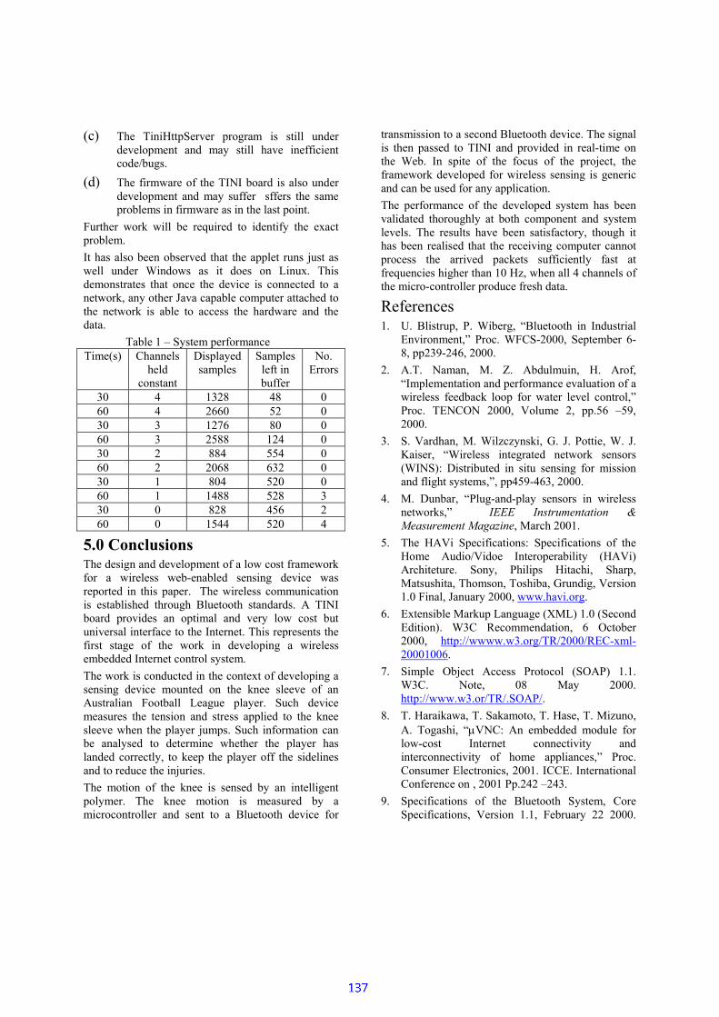
(c) The TiniHttpServer program is still under development and may still have inefficient code/bugs.

(d) The firmware of the TINI board is also under development and may suffer sffers the same problems in firmware as in the last point.

Further work will be required to identify the exact problem. It has also been observed that the applet runs just as well under Windows as it does on Linux. This demonstrates that once the device is connected to a network, any other Java capable computer attached to the network is able to access the hardware and the data.

Table 1 – System performance Time(s) Channels

held constant

Displayed samples

Samples left in buffer

No. Errors

30 4 1328 48 0 60 4 2660 52 0 30 3 1276 80 0 60 3 2588 124 0 30 2 884 554 0 60 2 2068 632 0 30 1 804 520 0 60 1 1488 528 3 30 0 828 456 2 60 0 1544 520 4

5.0 Conclusions The design and development of a low cost framework for a wireless web-enabled sensing device was reported in this paper. The wireless communication is established through Bluetooth standards. A TINI board provides an optimal and very low cost but universal interface to the Internet. This represents the first stage of the work in developing a wireless embedded Internet control system. The work is conducted in the context of developing a sensing device mounted on the knee sleeve of an Australian Football League player. Such device measures the tension and stress applied to the knee sleeve when the player jumps. Such information can be analysed to determine whether the player has landed correctly, to keep the player off the sidelines and to reduce the injuries. The motion of the knee is sensed by an intelligent polymer. The knee motion is measured by a microcontroller and sent to a Bluetooth device for

transmission to a second Bluetooth device. The signal is then passed to TINI and provided in real-time on the Web. In spite of the focus of the project, the framework developed for wireless sensing is generic and can be used for any application. The performance of the developed system has been validated thoroughly at both component and system levels. The results have been satisfactory, though it has been realised that the receiving computer cannot process the arrived packets sufficiently fast at frequencies higher than 10 Hz, when all 4 channels of the micro-controller produce fresh data.

References 1. U. Blistrup, P. Wiberg, “Bluetooth in Industrial

Environment,” Proc. WFCS-2000, September 6-8, pp239-246, 2000.

2. A.T. Naman, M. Z. Abdulmuin, H. Arof, “Implementation and performance evaluation of a wireless feedback loop for water level control,” Proc. TENCON 2000, Volume 2, pp.56 –59, 2000.

3. S. Vardhan, M. Wilzczynski, G. J. Pottie, W. J. Kaiser, “Wireless integrated network sensors (WINS): Distributed in situ sensing for mission and flight systems,”, pp459-463, 2000.

4. M. Dunbar, “Plug-and-play sensors in wireless networks,” IEEE Instrumentation & Measurement Magazine, March 2001.

5. The HAVi Specifications: Specifications of the Home Audio/Vidoe Interoperability (HAVi) Architeture. Sony, Philips Hitachi, Sharp, Matsushita, Thomson, Toshiba, Grundig, Version 1.0 Final, January 2000, www.havi.org.

6. Extensible Markup Language (XML) 1.0 (Second Edition). W3C Recommendation, 6 October 2000, http://wwww.w3.org/TR/2000/REC-xml-20001006.

7. Simple Object Access Protocol (SOAP) 1.1. W3C. Note, 08 May 2000. http://www.w3.or/TR/.SOAP/.

8. T. Haraikawa, T. Sakamoto, T. Hase, T. Mizuno, A. Togashi, “µVNC: An embedded module for low-cost Internet connectivity and interconnectivity of home appliances,” Proc. Consumer Electronics, 2001. ICCE. International Conference on , 2001 Pp.242 –243.

9. Specifications of the Bluetooth System, Core Specifications, Version 1.1, February 22 2000.

138

Experimenting with Jini Technology in Management of Small Networked Devices

Peter J Vial, Parviz Doulai and Rueben Bardak

School of Electrical, Computer & Telecommunications Engineering University of Wollongong

Wollongong, Australia

Abstract: The Internet will be facing an explosion in the number of small network enabled devices providing different services to Internet users in the near future. Many of these devices will have unique network layer and hence network administrators will have greater challenges in management of local networks. Sun Microsystems have proposed and implemented Jini services, which use Java to allow the interconnection of many devices and services on the Internet. This paper explores the feasibility of Jini Technology on a local Ethernet network, and demonstrates an experimental setup in which Jini simple services are used on a TINI (Tiny InterNet Interface) board. TINI technology allows connection of a wide variety of hardware devices to networks. The idea of “Jini over TINI” is explained in the context of smart Internet environment where the connectivity is incorporated into a wide range of devices. “Jini over TINI” has a huge potential to actively participate in the future smart Internet technologies.

1 Introduction: Networked Devices and Systems Part of the future smart Internet technology will be the explosion in the number of small Internet connected programmable devices providing different services to Internet users. These services may range from providing access to local or remote printers, scanners and photocopiers to remote data loggers, small Java based Web servers or small remote network monitors. Many of these devices will have unique network layer and network managers/administrators will have greater problems configuring the local networks. This is due to the large number of such devices that will be eventually connected to the network, as users demand the services they can provide. The smart technologies of the future Internet will surely include facilities which provide plug and play capabilities. Small intelligent, Internet aware devices will continuously be connected to the Internet, especially in Local Area Networks and Storage Area Networks. As users connect these devices to the network there will be a need for more network layer addresses which are most likely to be provided by IPv6 technology. This also requires more time from network administrators to account for, maintain and remove redundant devices from the network. In addition, these intelligent Internet aware devices will be capable of having their software updated, in a similar way that workstations need to have the latest patches applied

for security and enhanced service attributes. As the network grows in size, more administration tasks will be required to maintain and enhance the services provided by the local and remote network via these attached devices. This will add even more to the burden experienced by the network administrators and hence increase the maintenance costs of the network. One solution to this dilemma is for the device to recognise that an update for its services is available, and automatically fetch this update without the need for an administrator to intervene. Sun Microsystems have proposed and implemented Jini services, which use Java to allow the interconnection of many devices and services on the Internet [1]. Another relatively new product that allows the connection of any devices to the Internet is TINI (Tiny InterNet Interface) [2]. The idea of Jini over TINI suggests the connection of TINI, and hence a wide range of electronic systems, to the network using Jini services. With the leasing mechanism built into Jini the network manager no longer needs to worry about such devices, as they will be forgotten by Jini and not used if leases are not renewed.

139

This paper outlines the experiences in setting up and testing Jini services on a TINI board that is connected to a local Ethernet network. The paper also outlines the successes and problems encountered in getting the TINI to access its local hardware.

2 Jini and TINI Technologies

Jini is a network architecture of distributed systems. The Jini project started in 1995. The first vision of Jini project was the Jini technology will enable “plug and play” network just like the telephone network, and every device that is connected to the network can use the service provided. The Jini project was not announced to the public until January 1999 [3]. Jini is based on Java technology, and it uses its object-oriented features and also the mechanism referred to as Java “Remote Method Invocation (RMI)” to move objects around the network [4]. The objects like the service interface are travelling on the network using RMI. In fact RMI is a Java programming language-enabled extension to traditional remote procedure call mechanism. RMI provides an infrastructure for delivering services in a network. This particular infrastructure is very flexible [5]. It specifies a way for clients and services to find each other on the network and to accomplish a task together. It allows sharing services and resources over a network and provides access to these resources anywhere on the network [6]. The aim of Jini technology is to infuse flexibility into systems so that they are very scalable and adaptive to changes on the network [5]. These changes can be the addition of a new service (it will be automatically recognised by the network) or the failure of a network component which thus becomes unable to provide the service. In the later case, the distributed system should eventually forget about the failed device and no longer offer it as a possible service to Jini clients. As we shall see such mechanisms are built into Jini. TINI is an Internet aware programmable device with a cut-down Java Virtual Machine (JVM). It is capable of performing as a simple Web server, even though it has a maximum of 1 MEG in RAM. In fact a TINI board is simply a 1 MEG SIMM with a microcontroller and an Ethernet interface. Even so, it is a powerful device and a forerunner of devices that will supersede it in power and performance while remaining relatively an inexpensive system. Jini itself requires two facilities to operate which are currently only available in beta versions of the

TINI operating system. These are serialisation and Remote Methods Invocation. These facilities are not expected to be available until at the earliest early 2003. An organisation dedicated to providing Jini type services to resource constrained devices has produced a package called JMatos [7] which will execute on the TINI as a Web server providing Jini services, both lookup and client services are provided by this package which requires version 1.02d of the TINI operating system. It has a low memory footprint, requiring a maximum of 150kBytes of RAM. The software development kit is freely available for educational and research purposes on TINI as well as on Windows and Linux platforms [7].

2.1 Components of a Jini System The main components of a Jini system are the client, the service and the look-up service. Figure 1 shows a schematic representation of a Jini system. To make a service available for a client, the client has to ask the look-up service if such a service is available and where to find it. This implies that all services are registered in the look-up service.

Figure 1: Schematic Representation of Lookup, Service and Client in Jini technology [4]

The main advantage of a Jini architecture is that it is what we could call plug-and-play and configures itself automatically. When a new service arrives on a network, it is not registered anywhere. So the service has to find a look-up service in which it is going to register itself. The service doesn’t know the location of the look-up service. Therefore it has to find it through a process called discovery (step 1). Once the service has found the look-up service, the service registers itself in the look-up service by sending a service proxy, which actually is the interface of the service class (step 2). When a client needs a service, the client has to discover the look-up service as well (step 3). This is done through the same discovery process as the service) and then asks this look-up service if the

LookupService

ServiceProxy

NetworkService

ServiceProxy

NetworkClient 3

4

1 2

5

6

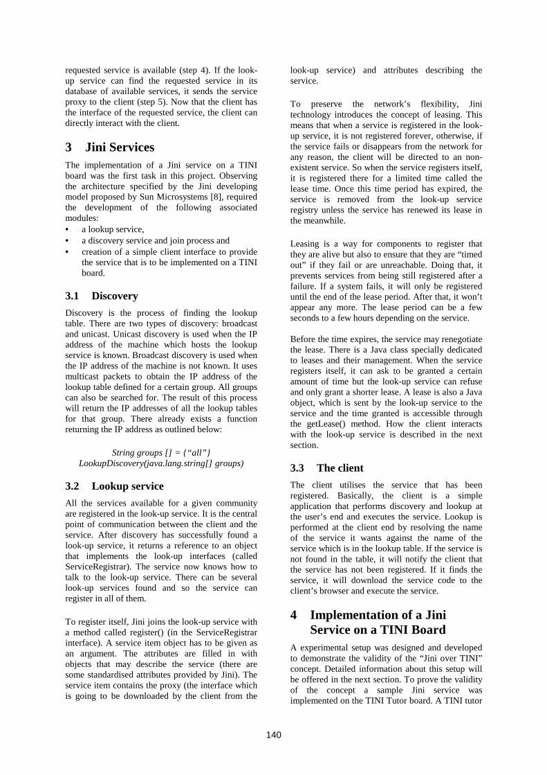
140

requested service is available (step 4). If the look-up service can find the requested service in its database of available services, it sends the service proxy to the client (step 5). Now that the client has the interface of the requested service, the client can directly interact with the client.

3 Jini Services The implementation of a Jini service on a TINI board was the first task in this project. Observing the architecture specified by the Jini developing model proposed by Sun Microsystems [8], required the development of the following associated modules: • a lookup service, • a discovery service and join process and • creation of a simple client interface to provide

the service that is to be implemented on a TINI board.

3.1 Discovery Discovery is the process of finding the lookup table. There are two types of discovery: broadcast and unicast. Unicast discovery is used when the IP address of the machine which hosts the lookup service is known. Broadcast discovery is used when the IP address of the machine is not known. It uses multicast packets to obtain the IP address of the lookup table defined for a certain group. All groups can also be searched for. The result of this process will return the IP addresses of all the lookup tables for that group. There already exists a function returning the IP address as outlined below:

String groups [] = “all” LookupDiscovery(java.lang.string[] groups)

3.2 Lookup service All the services available for a given community are registered in the look-up service. It is the central point of communication between the client and the service. After discovery has successfully found a look-up service, it returns a reference to an object that implements the look-up interfaces (called ServiceRegistrar). The service now knows how to talk to the look-up service. There can be several look-up services found and so the service can register in all of them. To register itself, Jini joins the look-up service with a method called register() (in the ServiceRegistrar interface). A service item object has to be given as an argument. The attributes are filled in with objects that may describe the service (there are some standardised attributes provided by Jini). The service item contains the proxy (the interface which is going to be downloaded by the client from the

look-up service) and attributes describing the service. To preserve the network’s flexibility, Jini technology introduces the concept of leasing. This means that when a service is registered in the look-up service, it is not registered forever, otherwise, if the service fails or disappears from the network for any reason, the client will be directed to an non-existent service. So when the service registers itself, it is registered there for a limited time called the lease time. Once this time period has expired, the service is removed from the look-up service registry unless the service has renewed its lease in the meanwhile. Leasing is a way for components to register that they are alive but also to ensure that they are “timed out” if they fail or are unreachable. Doing that, it prevents services from being still registered after a failure. If a system fails, it will only be registered until the end of the lease period. After that, it won’t appear any more. The lease period can be a few seconds to a few hours depending on the service. Before the time expires, the service may renegotiate the lease. There is a Java class specially dedicated to leases and their management. When the service registers itself, it can ask to be granted a certain amount of time but the look-up service can refuse and only grant a shorter lease. A lease is also a Java object, which is sent by the look-up service to the service and the time granted is accessible through the getLease() method. How the client interacts with the look-up service is described in the next section.

3.3 The client The client utilises the service that has been registered. Basically, the client is a simple application that performs discovery and lookup at the user’s end and executes the service. Lookup is performed at the client end by resolving the name of the service it wants against the name of the service which is in the lookup table. If the service is not found in the table, it will notify the client that the service has not been registered. If it finds the service, it will download the service code to the client’s browser and execute the service.

4 Implementation of a Jini Service on a TINI Board

A experimental setup was designed and developed to demonstrate the validity of the “Jini over TINI” concept. Detailed information about this setup will be offered in the next section. To prove the validity of the concept a sample Jini service was implemented on the TINI Tutor board. A TINI tutor

141

board is a special socket that holds the TINI and provides more elaborate Input/Output interfaces. Also available is most of the Java code for the program [8,9]. Other relevant projects include the implementation of Jini technology in devices such as disk drives, printers, scanner, etc as outlined in [3,8].

To modify and put associated programs into one program the software provided by the TINI and TINI Tutor board manufacturer was used [2,11]. Other software used included JMatos from PsiNaptic [7]. This software allows full Jini technology compatibility in small files (less than 150 KB). This is important as TINI has limited resources. Initially a 512 KB SIMM TINI board was used, but because of memory problems it was upgraded to a 1 MB SIMM.

4.1 The Service Provider and TINI Environment

Similar to Jini, the TINI is based on Java technology. In order to run the service, it was necessary to use the Java language. First, before this can be used, the TINI board needs to have the TINI firmware installed. After the firmware has been installed, then communication with the TINI through the network interface by setting the IP address for the TINI board is possible. After that the software for JMatos needs to be installed. As indicated earlier, the JMatos software provides fullJini technology on small embedded processors with limited resources. JMatos software enables a HTTP Server on the TINI board, so the client can transmit the service proxy through the HTTP Server. Jmatos also provides a Lookup Service, and a simple sample service that was modified to a simple service on TINI.

5 Experimental Testbed The experimental test-bed is shown in Figure 2. The following components are found in the experimental test-bed: 1. The TINI Tutor Board that is a special purpose

socket, provided with Input/Output such as an LCD display, serial ports, digital to analog converter (DAC), analog to digital converter (ADC), DIP switch/digital input, and digital outputs with LED indicators. The main purpose of TINI Tutor Board is to provide a useful real world outputs that could be connected to sensors, printers, cameras etc. In this experimental setup, it is used to toggle the LEDs ON and OFF [7]. The TINI Tutor Board has eight LEDs: 2 reds, 4 yellow, and 2 green. as shown in the top left hand corner of Figure 2. The software provided by [7] includes special Java classes which allow the status of these LEDs to be changed. The code which turns ON the second red LED looks like the following::

LEDManip manip = new LEDManip(); manip.add(LEDManip.R2);

2. JMatos, provided by the vendor for Jini services [7], allows the setup of client and lookup services. These were installed on the TINI.

3. Jini services were installed on a PC workstation running Windows 2000. The code for these services were downloaded from [8]. This was setup on the PC and used in the Jini experimental setup.

In order for services to be run on the TINI board, the following needs to be installed: • Jmatos • FileServer used to download the service proxy • The service class files

Figure 2: Experimental Setup

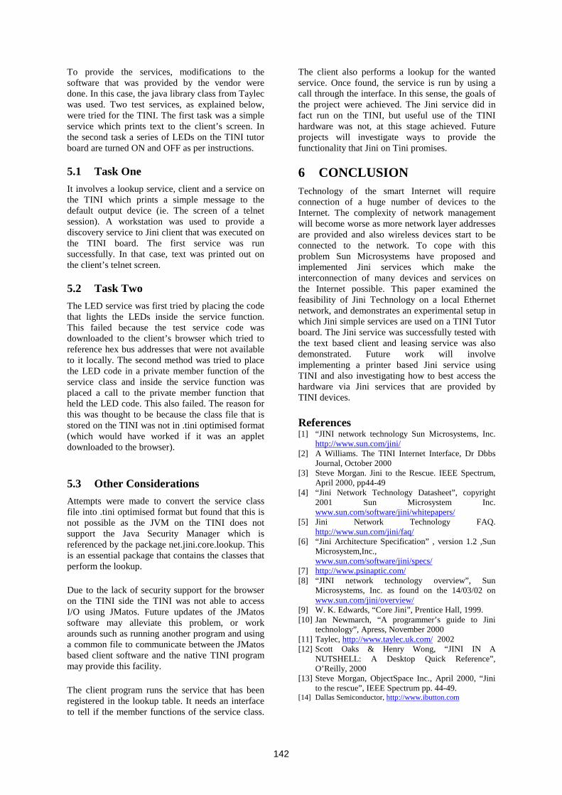
142

To provide the services, modifications to the software that was provided by the vendor were done. In this case, the java library class from Taylec was used. Two test services, as explained below, were tried for the TINI. The first task was a simple service which prints text to the client’s screen. In the second task a series of LEDs on the TINI tutor board are turned ON and OFF as per instructions.

5.1 Task One It involves a lookup service, client and a service on the TINI which prints a simple message to the default output device (ie. The screen of a telnet session). A workstation was used to provide a discovery service to Jini client that was executed on the TINI board. The first service was run successfully. In that case, text was printed out on the client’s telnet screen.

5.2 Task Two The LED service was first tried by placing the code that lights the LEDs inside the service function. This failed because the test service code was downloaded to the client’s browser which tried to reference hex bus addresses that were not available to it locally. The second method was tried to place the LED code in a private member function of the service class and inside the service function was placed a call to the private member function that held the LED code. This also failed. The reason for this was thought to be because the class file that is stored on the TINI was not in .tini optimised format (which would have worked if it was an applet downloaded to the browser).

5.3 Other Considerations Attempts were made to convert the service class file into .tini optimised format but found that this is not possible as the JVM on the TINI does not support the Java Security Manager which is referenced by the package net.jini.core.lookup. This is an essential package that contains the classes that perform the lookup. Due to the lack of security support for the browser on the TINI side the TINI was not able to access I/O using JMatos. Future updates of the JMatos software may alleviate this problem, or work arounds such as running another program and using a common file to communicate between the JMatos based client software and the native TINI program may provide this facility. The client program runs the service that has been registered in the lookup table. It needs an interface to tell if the member functions of the service class.

The client also performs a lookup for the wanted service. Once found, the service is run by using a call through the interface. In this sense, the goals of the project were achieved. The Jini service did in fact run on the TINI, but useful use of the TINI hardware was not, at this stage achieved. Future projects will investigate ways to provide the functionality that Jini on Tini promises.

6 CONCLUSION Technology of the smart Internet will require connection of a huge number of devices to the Internet. The complexity of network management will become worse as more network layer addresses are provided and also wireless devices start to be connected to the network. To cope with this problem Sun Microsystems have proposed and implemented Jini services which make the interconnection of many devices and services on the Internet possible. This paper examined the feasibility of Jini Technology on a local Ethernet network, and demonstrates an experimental setup in which Jini simple services are used on a TINI Tutor board. The Jini service was successfully tested with the text based client and leasing service was also demonstrated. Future work will involve implementing a printer based Jini service using TINI and also investigating how to best access the hardware via Jini services that are provided by TINI devices. References [1] “JINI network technology Sun Microsystems, Inc.

http://www.sun.com/jini/ [2] A Williams. The TINI Internet Interface, Dr Dbbs

Journal, October 2000 [3] Steve Morgan. Jini to the Rescue. IEEE Spectrum,

April 2000, pp44-49 [4] “Jini Network Technology Datasheet”, copyright

2001 Sun Microsystem Inc. www.sun.com/software/jini/whitepapers/

[5] Jini Network Technology FAQ. http://www.sun.com/jini/faq/

[6] “Jini Architecture Specification” , version 1.2 ,Sun Microsystem,Inc., www.sun.com/software/jini/specs/

[7] http://www.psinaptic.com/ [8] “JINI network technology overview”, Sun

Microsystems, Inc. as found on the 14/03/02 on www.sun.com/jini/overview/

[9] W. K. Edwards, “Core Jini”, Prentice Hall, 1999. [10] Jan Newmarch, “A programmer’s guide to Jini

technology”, Apress, November 2000 [11] Taylec, http://www.taylec.uk.com/ 2002 [12] Scott Oaks & Henry Wong, “JINI IN A

NUTSHELL: A Desktop Quick Reference”, O’Reilly, 2000

[13] Steve Morgan, ObjectSpace Inc., April 2000, “Jini to the rescue”, IEEE Spectrum pp. 44-49.

[14] Dallas Semiconductor, http://www.ibutton.com

!"#$ %'&%($)%

*,+.-0/21436587:9;=<43?>A@BC;EDGF'HI5KJL+M3NO3?>?>03P1CQ

RTSVUXWAYZWA[=WP\^]`_bac(\Lde\If?_bgg[=S2Y.f?hWAYZ_bSiUGjk\IUX\lha6f6mn^S2YeoC\LapUXYeWrq_I]tsC_u[=WAmwv^[iUrWAa6hIdeYxhyzhLOUX_bSw|(hC\IU^sEv~ubu~v^[iUrWAa6hIdeYxh

yzhIYedgYeC\IhUrq4dKoYe\IUr=aAYdK\Lou\Ld.U?[2S=Y.UPh4\l4[(hI[

1C;bXBC>P</2+er3

^\L=W_]dZ\IfWAaPY.fLhId'hSidZ\IfWPaA_bS2Y.fS= 2v\Ld.hIY.4\n^S=YZoC\La6UrYeWrq

v4\LdxhY.\¡sv ~ubb¢v^[iUXWPa6hIdeY.hyzhIYedG|(hIS= =¤£¥m=YeWP\bhb4\d.hYx4\C¤\I4[(¦h[

§^¨k©ªG«^§^¬ª­.®¯M°I±²O³u´0³uµr¶A·¸8µ³I¶Mµr²`µX®¯´¶`¹?º»I²`¯¼LµP½Tµr®L¯`¶´0¾±¦²MµP¼¿ µX¯`°I¹I¼^ÀZ¹¶iÁ¹?±®L¯`¾Â³uµX¶.ÀZ¹¶ ¿ ±®IýM°u´6®I®µr¾iµr²M¯`± ¿ ´0¯`±¹?®´6®b¼½¾¹?²MµP¼¾¹L¹?³¡³u¹6¸8µr¶G½¹?®L¯M¶`¹?¾4ÀZ¹¶¯M°Iµ¶MµrÄ?µX¶`²`µk¾±®IŹ6À'Æ(ÇÈÉz®IµX¯.¸'¹¶`ÅL²PÊ(ËÌ»I¶ ¿ µr¯`°¹l¼E·Lºu´6²MµP¼¹?®¾±®IµP´0¶Í »u´?¼l¶´6¯M±K½½¹®L¯`¶`¹¾i²`ÂL²M¯`µ ¿ ²Î¯M°Iµr¹¶`´6®u¼Ï´6¾ ¿ ´0®OÐb¾¤Ñ¯`µX¶`±®IÃu·i¼l¹µX²k®I¹?¯G¶Mµ Í »I±¶`µ´6®L¯`¶´6±®I±®IòM ¿ ºb¹?¾²ÌÀZ¹¶½M°u´6®®Iµr¾¹¶ÒL±Ã?®u´0¾C¯`¹t­.®L¯`µr¶ÓÀZµr¶`µX®u½µOÔ´0¯`±¹kÕ.ÒL­`ÔÖ8µr²M¯`±Ñ¿ ´0¯`±¹?®4Ê×(°µ ¿ ´0±®±®L¯`µX¶`µr²M¯k¹6À(¯`°I±²G®IµX¸Ø²½M°Iµ ¿ µ^±²¯`°b´6¯k±¯± ¿ ³I¶`¹6ĵr²G¯`°µ³uµX¶.ÀZ¹¶ ¿ ´0®u½µ^¹6À½»I¶M¶`µr®L¯Òl­`Ôºu´0²`µP¼^³b¹6¸'µr¶½T¹?®L¯`¶M¹?¾¯MµP½M°I®I± Í »Iµr²Ì¸(°I±¾¦µ´AÄ?¹±Ù¼l±¦®ÃG¯`°Iµ³I¶M¹?ºI¾µ ¿ ¹6À³b¹6¸'µX¶µr²½X´6¾K´6¯M±¦¹®·Ì¸(°I±K½`°±²¹6Àe¯`µr®¹?ºLѲ`µX¶`Ä?µA¼±®Ú½T»I¶`¶Mµr®L¯²`ÂL²M¯`µ ¿ ²PÊ

ÛbÜÝPÞ ªG«^ß!àᡬGª Ý ß Þâ(³lÑx¾±®IÅã¹6¸8µr¶OÆ8¹®¯M¶`¹¾Õ.ãiÆ(Öt±²!´½¶`»b½±K´6¾(µr¾µ ¿ µr®L¯±® ¿ »I¾¯M±i»I²`µX¶Æ(ÇÈÉä²`ÂL²`¯Mµ ¿ ²AÊ­.®¹?¶¼Lµr¶k¯M¹ ¿ ´AåLѱ ¿ ±²`µ½r´6³b´?½±¯.´6®u¼çæ»b´6¾±¯.¹6ÀÒLµX¶`ÄL±K½µÕ.æ̹ÒIÖX·è´0¾¾È¹ºI±¾¦µÒL¯´0¯`±¹?®Õ.ÈÒIÖt¯M¶´6®² ¿ ±²M²`±¹?®I²²`°I¹»I¾K¼ºbµ¶MµÑ½µr±ÄµP¼´0¯(¯`°Iµké8´6²`µkÒL¯´6¯`±¹®Õ.é'ÒÖ¸(±¯M°µ Í »b´6¾=³u¹6¸8µr¶êë ·ìXí`ÊÒL±®u½Tµ!Æ(ÇÈÉî²`ÂL²M¯`µ ¿ ²´0¶`µt±®¯Mµr¶.Àeµr¶`µr®b½µO¾± ¿ ѱ¯`µP¼E· ¿ »b½`°^¸'¹¶`Ž¹®u½µr®L¯`¶´6¯Mµr²G¹?®¯M°Iµ!Òl±¦Ã®u´6¾C¯M¹O­.®Lѯ`µX¶.ÀZµr¶Mµr®u½µtÔ´6¯M±¹kÕxÒL­`ÔÌÖ'´0²è´ ¿ µP´0²`»I¶Mµ¯`¹k½¹®¯M¶`¹¾ïÈÒ³b¹6¸'µr¶M² êñð ·Lòu·Ió·IôAí`Ê­.®¯`°Iµr¹¶`ÂL·(´6²`²M» ¿ ±®Ióbµr¶.ÀZµA½¯Å®¹6¸(¾¦µA¼LÃ?µ^¹6ÀG¯`°IµÒL­`Ô·èÒl­`Ôõºb´6²`µA¼zãiÆ¥¹»I¯`³bµr¶.Àe¹?¶ ¿ ²²`±Ã?®u´0¾²`¯`¶Mµr®Iï`°ºu´0²`µP¼ãiÆÊ(×(°I±²^±¦²^ºuµA½r´6»I²Mµ¯M°Iµ³b¹6¸8µr¶¹6À¯M°Iµ¶MµÑ

½µr±ÄµP¼²M±Ã?®u´0¾±²O±®Àx´?½T¯¯M°Iµ²M» ¿ ¹6À¯M°Iµ³u¹6¸8µr¶O¹0À¯`°µ¼Lµr²`±¶MµP¼k´6®u¼¯`°µ'±®L¯`µr¶ÓÀZµr¶Mµr®u½µÌ²`±Ã?®u´0¾²PÊ4×(°Iµr¶`µTÀZ¹?¶Mµ?·±®¢´¡²`±¯`»b´6¯`±¹®¸(°Iµr¶Mµ¯`°Iµ¶`µA½µr±Ä?µP¼²`±Ã?®u´0¾'³b¹6¸8µr¶k±²²`¯M¶`¹®IÃGºbµP½r´6»²`µ¯`°Iµ(±®L¯`µX¶.ÀZµr¶Mµr®u½µ±²=²`±Ã?®±¤ÐC½r´6®L¯P·´²`±Ã6Ñ®u´0¾²`¯M¶`µr®Ã?¯`°¡ºu´6²MµP¼³b¹6¸'µr¶½¹?®L¯M¶`¹?¾=´6¾Ã?¹¶`±¯`° ¿ ¸'¹»I¾K¼¸(¶`¹®IÃ?¾Â±®I²M¯`¶M»u½¯t¯`°IµÈÒ¯`¹¼lµP½¶`µA´6²`µ±¯`²t¯`¶´6®I² ¿ ±¯³b¹6¸'µr¶AÊO×(°µr¶`µÀe¹?¶`µ·iÒL­`Ôö²`µrµ ¿ ²G¯`¹¡ºuµO´ ¿ ¹?¶Mµ®u´0¯`»LѶ´0¾(³u´6¶´ ¿ µr¯`µr¶¯`¹½¹?®L¯`¶M¹?¾(±®L¯`µr¶ÓÀZµr¶Mµr®u½µ¾± ¿ ±¯MµP¼²MÂL².ѯ`µ ¿ ²PÊ^÷(¹6¸8µrÄ?µr¶A·2Òl­`Ôøºb´6²`µA¼ãiÆö±¦²G´0²`²`¹I½±K´0¯`µP¼"¸(±¦¯M°ì ¿ ´rÁ¹¶¼L¶´A¸(ºu´½MŲAÊGù4±¦¶M²`¯M¾¦ÂL·CÒL­`Ôz±²G¼L±ú½»I¾¯(¯M¹µX².ѯ`± ¿ ´6¯`µO´½r½»I¶´6¯Mµr¾Â êñû í`ÊâÈÚ×Ò êñü í²`³bµP½±Ðuµr²²`± ¿ »I¾Ñ¯´0®Iµr¹»I²(¯`¶´6®I² ¿ ±²`²M±¦¹®¹0À2¯M°IµGÇÎãýÆ(Æ(÷½¹®L¯`¶`¹¾ï½M°u´0®LÑ®Iµr¾ý¸(±¦¯M°ÇãiÇÆ(÷î¼I´0¯´O½M°u´0®I®Iµr¾.ÊkÒL­`Ôö±²µr²`¯M± ¿ ´6¯MµP¼»I²M±¦®Ã³I±¾¦¹¯º±¦¯M²k¯`¶´6®I² ¿ ±¯`¯MµP¼¹?®ÇãiÆ(Æ(÷GÊ8ÒLÂL²`¯`µ ¿½r´0³u´?½±¯.±²^¹?ºLÄL±¦¹»I²`¾Â¶`µP¼L»b½µP¼ø´½r½¹¶¼L±®Iþ¦ÂLÊîÆ8µr®Lѯ`¶´6¾±²`µP¼²½M°Iµ ¿ µX²P·¸(°Iµr¶Mµ¯M°Iµé'Ò,°u´6²±®LÀZ¹¶ ¿ ´6¯`±¹®þbÿ eÿ ÿ ÿ

! ÿ#"$%&'(*)+ eÿ,"-. /!021$(-331$45-67

ÀZ¹¶´6¾¾kÈÒC·½r´6®ø¼LµX¯`µr¶ ¿ ±®Iµ¢Òl­`Ô ¿ ¹¶`µ´?½r½»¶´6¯Mµr¾Â¯`°b´6®¼L±²`¯M¶`±ºI»I¯MµP¼²`ÂL²M¯`µ ¿ ² ê óXí`Êi÷ ¹6¸'µrĵr¶P·b½µr®L¯`¶´6¾±²`µP¼¿ µX¯`°I¹I¼L²´6¶Mµ¼L±ú½»I¾¯O¯M¹± ¿ ³I¾µ ¿ µX®¯O¼l»Iµ¯M¹¯`°Iµr±¶°I±Ã?°½¹ ¿ ³I»¯´6¯M±¹?®u´0¾u½¹ ¿ ³I¾µåI±¯.ÂÊ×(°Iµk¹¯`°IµX¶ ¿ ´rÁT¹?¶¼L¹6¸(®LÀ.´6¾¾=¹6ÀÒL­`Ôöºu´6²MµP¼ãiÆö±²

¯`°µ³I¶M¹?ºI¾µ ¿ ¹6ÀC³b¹6¸'µr¶8µr²½r´6¾K´6¯M±¹?®Ê=ÒL­`ÔG·´6²i¯M°Iµ®u´ ¿ µ²`»Ã?Ã?µX²`¯`²A·L±²2´Ì¶´0¯`±¹ºbµr¯.¸8µrµr®O²M±Ã?®u´0¾´6®b¼G±®L¯`µr¶ÓÀZµr¶Mµr®u½µ?Êɲ¹?®IµkÈÒ±®u½¶MµP´6²Mµr²±¯M²Î³b¹6¸8µr¶G¯`¹½¹ ¿ ³bµr®I²´6¯`µÀZ¹¶±®L¯`µr¶ÓÀZµr¶`µX®u½µÀZ¶M¹ ¿ ¹¯`°Iµr¶ÈÒL²A·(±¯`²k²`±Ã®u´6¾(±®L¯`µr¶ÓÀZµr¶Mµr²¿ ¹¶`µ¹?®´6¾¾¹¯`°Iµr¶ÈÒL²Ì¸(°I±K½`°¡¸(±¦¾¾4±¦®¯M»I¶`®±®u½T¶`µP´0²`µ¯`°µr±¶Î¯M¶´0®I² ¿ ±¦¯Ì³u¹6¸8µr¶AÊG­.®I²M¯´6º±¦¾±¯.´0®u¼¡³u¹6¸8µr¶µr²½X´AѾK´6¯M±¦¹®kÕx´0¾²`¹G¼LµÐu®µP¼k´6²i³b¹?²M±¯`±Ä?µýÀZµrµP¼lºu´?½MÅIÖi½r´0®¶Mµr²`»I¾¯¸(°I±¾µ(¯`°IµÒL­`ÔÀZ¹¶iµP´½`°ÈÒk¶Mµ ¿ ´0±®I²=¯`°IµÌ²´ ¿ µ?Ê4×(°I±²±²³u´0¶`¯M±Ù½T»I¾K´6¶`¾Â³I¶MµrÄ?´6¾µr®L¯¸(°µr®¯M°Iµt²`ÂL²`¯Mµ ¿ ±²¹³uµX¶.Ñ´6¯M±®Iô0¯¹?¶Ì®IµP´0¶Î¯M°Iµk½r´6³u´½±¯.¾± ¿ ±¯PÊý×(°Iµr¶`µTÀZ¹?¶Mµ?·2´0®ÒL­`Ô,ºu´6²MµP¼ãýÆz²½M°Iµ ¿ µt²`°I¹»I¾K¼ºuµt»I²MµP¼±®½T¹?®PÁ»®u½Mѯ`±¹®¸(±¦¯M°´Ú³uµr¶ÓÀZµP½¯k½r´0¾¦¾8´?¼ ¿ ±¦²M²`±¹?®½¹?®L¯`¶M¹?¾ ¿ µP½M°u´pÑ®I±² ¿ ·=¸(°I±K½M°±²kÄ?µr¶M¢¼L±ú½»¾¦¯¯`¹Ã?»b´6¶´0®L¯`µrµ±®¶MµP´6¾²`ÂL²M¯`µ ¿ ²PÊ

8b°u´0®IÃ:9;=<>? ê @ í´?¼¼L¶`µr²M²k¯`°Iµ^³u¹6¸8µr¶tµr²½X´6¾K´6¯M±¦¹®³I¶M¹?ºI¾µ ¿ ¸(±¦¯M°´=Á¹?±®L¯C²`±Ã®u´6¾L²`¯M¶`µr®Ã?¯`°O´0®u¼tÒL­`Ôºu´0²`µP¼ãiƲ½`°µ ¿ µ=¯`°b´6¯2½T¹ ¿ ³b´6¶`µX²uºb¹?¯M° Í »u´6®L¯`±¯M±¦µX²C¯`¹(¯`°¶`µr²M°Lѹ?¾K¼L²k´6®b¼¢´¼rÁ»I²M¯`²t³u¹6¸8µr¶k±®¯M°IµÈÒ¸(±¯M°¢´¡²`± ¿ ³I¾µ´?¼´6³I¯M±¦Äµ²`¯`µX³²`±BArµ´6¾Ã?¹¶`±¯`° ¿ Ê×(°Iµ¡³u¹²`±¯`±Ä?µ^ÀZµXµP¼Ñºu´½`Åk³b¹?¯Mµr®L¯`±K´6¾C±²8¹6Ài½¹?»I¶M²`µµr¾± ¿ ±®u´0¯`µP¼¸(±¯`°O¯M°Iµ»I²`µ¹6À¯`°Iµ²M±¦Ã®u´6¾(²M¯`¶Mµr®IÃ?¯M°½¹®I²`¯M¶´6±®L¯PÊ×(°I±²O´6³³I¶`¹L´?½M°¿ ´A¡²`¯`¹³¯`°Iµ^µr²½X´6¾K´6¯M±¦¹®³I¶`¹ºI¾µ ¿ ºI»I¯G±¯G²M¯`±¾¾'¼L¹Lµr²®I¹¯ ¿ ±®I± ¿ ±²`µ(¯M°IµkÈÒ^¯`¶´0®I² ¿ ±¯(³u¹6¸8µr¶PÊÌÔ´6¯´6®u´ ¿ ´pÑ°u´0¯´6®b´C9;D<>? êë$E í³¶`¹?³b¹?²Mµ´"²`± ¿ ³¾¦µ ¿ µr¯`°I¹I¼"ÀZ¹¶µåI¯`¶´?½¯M±®IÃÌÀZ¶`¹ ¿ ¯M°Iµ'¶MµP½µr±ÄµP¼G²M±Ã?®u´0¾x·A¯M°Iµè¼lµr²`±¶`µA¼´0®u¼±®L¯`µr¶ÓÀZµr¶`±®IÃ̲`±Ã?®b´6¾6²`¯M¶`µr®Ã?¯`°²2»²`±®IÃ(³I±¾¹?¯b²` ¿ ºb¹?¾²PÊb×(°I±²¿ µX¯`°I¹I¼C·6°¹6¸'µrĵr¶P·¶`µA¼L»u½µr²8²`ÂL²M¯`µ ¿ ½r´0³u´?½±¯.´0®u¼t°u´0²³b¹?¯`µX®¯M±K´6¾?³¶`¹?º¾¦µ ¿ ²C¸(°Iµr®tãiƺ±¦¯M²2´0¶`µi±®µr¶`¶M¹?¶4¹?®¯`°IµÀZ¹¶`¸(´6¶¼½M°u´0®I®Iµr¾.Êæ´6±®´0®u¼GFG´rÁ±K½ êë?ë íi¯´6Å?µt¯`°µk³u¹6¸8µr¶µr²½X´6¾K´6¯M±¦¹®

³I¶M¹?ºI¾µ ¿ ÀZ»I¶`¯M°Iµr¶=ºL´6³³I¾Â±®IÃ(²M¯`¹I½M°u´6²M¯`±K½(½¹®¯M¶`¹¾²MÂL².ѯ`µ ¿ ²O¯M°Iµr¹¶`¯`¹ÒL­`Ôäµr²`¯M± ¿ ´6¯M±¹?®¢´0®u¼ãiÆÊ(ÒL­`ÔäµX¶.Ѷ`¹¶G´6®u¼ÈÒ¯M¶´6®² ¿ ±¯Ì³u¹6¸8µr¶G´6¶MµèÁ¹±®¯M¾Â ¿ ±®I± ¿ ±²`µA¼´6®b¼¢´0®÷7H Ðb¾¦¯Mµr¶JI0µr²`¯M± ¿ ´6¯M¹?¶t±²k»I²`µP¼ç¯`¹¯M¶´½`ů`°Iµ½M°u´6®®Iµr¾CÄ?´6¶M±K´6¯`±¹®I²PÊ4×(°IµrÂkµåI¯Mµr®u¼^¯`°IµX±¦¶8¸8¹?¶`ÅkºLÂk´6³LѳI¾ÂL±®Iý¹®I²`¯M¶´6±®IµA¼¹³I¯`± ¿ ±¦²´6¯M±¦¹®¯`µA½`°®I± Í »µr²k¯`¹±®Lѽ¾»u¼Lµ ¿ ´AåI± ¿ » ¿ ´0®u¼ ¿ ±®I± ¿ » ¿ ´6¾¾¹6¸'µA¼È¡Ò¯M¶´6®².Ñ¿ ±¯8³u¹6¸8µr¶AÊi×(°I±²¸8¹?¶MÅO±²8ÀZ¹¾¦¾¹6¸8µP¼k»³±® êë ìXí=¸(°Iµr¶`µ¯`°µÒL­`Ô¥µr¶M¶`¹¶Ä?´6¶M±Ù´0®u½µ´0®u¼ç²`» ¿ ¹0À!¯M°IµÄ?´0¶`±K´6®b½µ¹6ÀOÈÒ¯M¶´6®² ¿ ±¯M±¦¹®³b¹6¸'µr¶´6¶`µOÁT¹?±®L¯`¾Â ¿ ±®I± ¿ ±¤²MµP¼CÊKC±®IµA´6¶GæÌ»u´?¼L¶´6¯M±Ù½t½¹®¯M¶`¹¾i¯`°IµX¹?¶`¡±¦²G´0³I³I¾±µP¼CÊG÷(¹6¸8ѵrĵr¶P·L¯M°I±² ¿ µr¯M°I¹I¼G±²i®¹?¯i²M»I±¯´6º¾¦µ8Àe¹?¶=¯`¶´?½MÅL±¦®Ã½M°u´6®LÑ

®Iµr¾ÌÄ?´6¶M±Ù´0¯`±¹?®²!¼L»µ¯`¹¯M°Iµ ¿ ¹ºI±¾µk²`³bµrµP¼CÊ×(°I±²k±²P·°I¹6¸8µrÄ?µX¶P·u´t½¶M»u½±K´6¾4±¦²M²`»Iµ¯M¹kºuµG´?¼¼L¶`µr²M²`µP¼ÀZ¹?¶8Àx´¼L±®IýM°u´6®®Iµr¾²PÊ­.®k¯`°I±²=³u´0³uµr¶A·?¸8µ8³I¶`µr²Mµr®L¯è´Ì¶M¹?ºI»I²M¯'¼LµP½Tµr®L¯`¶´0¾±¦²MµP¼

¿ µX¯`°I¹I¼^ÀZ¹¶iÁ¹?±®L¯`¾Â³uµX¶.ÀZ¹¶ ¿ ±®IýM°u´6®I®µr¾iµr²M¯`± ¿ ´0¯`±¹?®´6®b¼½¾¹?²Mµ¾¦¹L¹³³b¹6¸'µr¶k½¹®¯M¶`¹¾8ÀZ¹?¶t¯`°Iµ¶MµrÄ?µr¶M²`µ¾±®IŹ6ÀiÆ(ÇÈÉ®µr¯.¸'¹¶`ÅL²Pʵ̺u´6²Mµ¹?»I¶(´6³I³¶`¹´½M°O¹?®^¹?³Lѯ`± ¿ ´6¾2½T¹?®L¯`¶M¹?¾8²`ÂL²`¯Mµ ¿ ²G¯M°Iµr¹¶`ÂLÊO×(°Iµ^®I¹6Ä?µX¾¦¯.¡¹6À(¹?»I¶´6³³I¶`¹L´?½M°±²Ì¯`°u´0¯Î¸(°±¦¾µG±¯´6± ¿ ²´0¯ ¿ ´6±®L¯´0±¦®±¤®IÃt¯`°IµÒL­`Ô¹0ÀµP´?½M°ÈÒk½¾¹?²Mµ¯`¹t¯`°µÎÒL­`Ô¯´6¶MÃ?µr¯M²P·L±¯`²i± ¿ ³I¾µÑ¿ µX®¯´6¯M±¦¹®¼L¹Lµr²G®I¹¯¶`µX¾¦Â¡¹?®¯`°Iµk´?½¯M»u´6¾i½r´0¾K½»I¾K´6¯M±¦¹®¹6À¯M°IµÒL­`ÔÊ?­.®k¹¯`°Iµr¶8¸8¹?¶¼l²P·¹?»I¶'´0³I³I¶M¹´?½M°k¯´6Å?µX² >B; > 8±¦®L¯M¹!´½r½¹?»®¯8¯`°µÎ±®L¯`µX¶.ÀZµr¶Mµr®u½µt½¹ ¿ ³u¹®Iµr®L¯'¹0ÀµP´½`°t²`±Ã®u´6¾LºI»I¯=±²®¹?¯i´CµP½¯MµP¼tºLÂG³u¹²`±¯`±Äµ=ÀZµrµP¼lºu´?½MÅCÊÉ®¹?¯`°µr¶=± ¿ ³u¹¶`¯´6®L¯IÀeµP´6¯M»I¶`µi¹0Àu¹?»¶C³I¶`¹³u¹²`µP¼ ¿ µr¯M°I¹I¼±²(¯`°u´0¯'±¯¼L¹Lµr²(®¹?¯8¶`µr¾ÂO¹®´6®LÂk³I±¾¹?¯i¹¶(¯`¶´0±®I±®IòMµÑÍ »Iµr®u½Tµ¯M°L»I²±®u½T¶`µP´0²`±®Iï`°Iµ^²`ÂL²`¯Mµ ¿ ½r´0³u´?½±¯.ÂLÊ×(°IµÃ?µX®Iµr¶´0¾u²M¯`¶M»u½¯`»¶`µ¹6À¯M°I±²'´6¾Ã?¹¶`±¯`° ¿ ±¦²ý²`± ¿ ±¾K´6¶C¯M¹G¯`°Iµ¹?®µ´0¾¶`µP´¼LÂO± ¿ ³¾¦µ ¿ µr®L¯`µA¼t±¦®^¯`°Iµ­`Ò @ ó²`ÂL²`¯Mµ ¿ Ê=­.¯Ì±²¯`°µr¶`µÀe¹?¶`µkĵr¶`µP´0²`¯M¹O± ¿ ³¾¦µ ¿ µr®L¯8±¦®¡³I¶´½¯`±K½r´0¾2²MÂL².ѯ`µ ¿ ²PÊ=ù4±®u´6¾¾Â·0ºuµr±®IÃt´6®´¼I´6³¯`±Ä?µ ¿ µr¯`°I¹I¼C·0±¦¯(´6¾¾¹6¸(²¯´0ÅL±¦®ÃO±®L¯`¹O´?½X½¹?»I®L¯ÌÀx´¼L±®IÃO½M°u´6¶´?½¯Mµr¶`±²`¯M±K½²¹0Ài¸(±¦¶MµÑ¾µr²`²½M°u´6®I®µr¾²PÊ(×(°I±²´¼I´6³I¯M±Ä±¯.Âk¯M¹O¯`°µ½M°u´6®I®µr¾2½¹®LѼL±¯`±¹®I²i±²=ÀZ»I¶M¯`°IµX¶'± ¿ ³¶`¹6Ä?µA¼ºLÂ!´ ¿ »¾¦¯M±L²`¯`µX³O²`±BArµ´6³LѳI¶M¹´?½M°·L¸(°±Ù½M°´6¾¾¹6¸(²'½¹ ¿ ³uµX®I²´0¯`±®IÃÀZ¹¶è¼lµrµr³^Àx´?¼lµr²PÊ­.®k¹?¶¼Lµr¶i¯M¹´?½M°I±µrĵ(¯`°I±²A·´ Í »u´6®L¯M±¦²MµP¼ ð Ñ.ºI±¯iãiƽ¹ ¿ Ñ¿ ´0®u¼¹?®¯M°IµÀZµXµP¼Lºu´½`Å,ÕKÀZ¹¶`¸(´6¶¼ÖO½M°u´6®®Iµr¾G±²O³¶`¹6ѳb¹?²`µA¼CÊk¯`°µk³u´6³bµr¶G±²¹?¶Mô6®±¦²MµP¼´6²ÌÀZ¹?¾¾¹6¸(² ¸'µtÐu¶M²`¯³I¶Mµr²`µr®L¯^¯`°Iµ³I¶M¹?ºI¾µ ¿ Àe¹?¶ ¿ »¾Ù´0¯`±¹?®´6®u¼"¯`°IµÃ?µX®Iµr¶´0¾¾±®IµP´6¶ Í »u´¼L¶´0¯`±K½iÃL´6±®k½¹?®L¯`¶M¹?¾¾µr¶PÊ4×(°Iµr®4·?¯M°Iµ½M°u´6®I®µr¾µr²M¯`± ¿ ´0¯`±¹?®^±¦²´¼I¼L¶Mµr²`²MµP¼»I²`±®IÃO´^Ï´6¾ ¿ ´0®tÐu¾¯`µr¶AÊù4±¤Ñ®u´0¾¦¾ÂL·b²`± ¿ »I¾K´6¯M±¦¹®I²½¹ ¿ ³u´0¶`±®IÃO¯M°IµO½¹®Äµr®L¯`±¹?®b´6¾i­`ÒÑ@ ó³b¹6¸'µr¶(½¹®¯M¶`¹¾¼LµrÄL±K½µ¸(±¦¯M°k¹?»I¶8³I¶M¹?³b¹?²`µA¼O²½M°Iµ ¿ µ´6¶Mµ³I¶`µr²Mµr®L¯`µP¼EÊ

CÜ «^ßk¨ ß!«zá8§ª Ý ß Þ­.®¯`°I±²G³u´0³uµX¶P·4¸'µt»I²`µk¯M°IµtÀZ¹¾¦¾¹6¸(±®IÃk®I¹¯´0¯`±¹?®I²G´0®u¼´6²M²`» ¿ ³I¯`±¹®I²

! #" Õ$Ö ±²¯`°µ¯M¶´6®² ¿ ±¯8³u¹6¸8µr¶Ì¹6À ¿ ¹?ºI±¾µ»I²Mµr¶&%¼L»I¶`±®IÃt¯`°µÀZ¶´ ¿ µ$PÊ

(')" Õ$Öý±²=¯`°IµÌ² Í »u´6¶MµP¼O´0ºI²`¹¾»I¯`µ(Ä?´0¾¦»µ(¹6ÀC¯`°Iµ´AÄ?ѵr¶´0Ã?µÕZ¹6ĵr¶tÀZ¶´ ¿ µ*$Öt¹0Àί`°µ»³LÑx¾±®IŽM°u´6®I®µr¾Ã´6±®¡ÕKÀZ¹¶'»I²Mµr¶%ÖrÊ

×(°Iµ=²`³I¶MµP´?¼L±®Iý¹I¼Lµr²=´6¶`µý¾¦¹®IÃ(¶´0®u¼L¹ ¿ ²`µ Í »IµX®u½µr²²`»u½M°G¯M°u´6¯4¯`°Iµ'½T¶`¹?²M²2½¹¶`¶Mµr¾K´6¯`±¹®I²ºbµr¯.¸8µrµr®t»I²`µr¶M²´AÄ?µr¶´6Ã?µA¼¹6ĵr¶´ýÀZ¶´ ¿ µ=´6¶Mµ'´6³I³¶`¹AåI± ¿ ´6¯Mµr¾Â ë+, ·¸(°Iµr¶`µ , ±²8¯`°Iµ²`³I¶MµP´?¼L±®IÃkÃL´6±®Ê

(-/. ±²C¯`°IµiÄ?´0¶`±K´6®b½µ=¹6ÀI¯`°Iµý¯`°Iµr¶ ¿ ´0¾6®I¹?±²`µý³I¶`¹I½µr²M²Õ ¿ ¹I¼LµX¾¦¾µP¼´0²´ ArµX¶`¹ ¿ µP´6® F´6»I²M²`±K´6®¶´6®u¼l¹ ¿Ä?´6¶`±K´0ºI¾µPÖrÊ

(01" Õ2$Ö43 5" Õ$Ö ')" Õ2$Öi±²i¯M°Iµ³b¹6¸'µX¶'¹0À¯`°IµÌ²`±Ã?®u´0¾.·¶`µP½µX±¦ÄµP¼´6¯Ì¯`°Iµtºu´0²`µt²`¯´0¯`±¹?®4·ï´pÀZ¯`µX¶¼lµr²`³I¶MµP´?¼Ñ±¦®ÃGÀZ¹¶'»²`µr¶6%CÊ7EÜ8 Ì«9:¬Gª ß&;<«¬tß Þ ªG«^ß=

â(²M±®IÃG¯`°µ´6ºb¹6Ä?µ(®I¹¯´6¯M±¹?®I²A·6¸'µ½X´6®k¸(¶`±¯Mµ(¯`°IµÒL±Ã?®u´0¾¯`¹k­.®L¯Mµr¶.ÀZµX¶`µr®u½TµÕZ³I¾»I²Ì®I¹?±²`µAÖÔ´0¯`±¹^ÕxÒL­`ÔÌÖ8ÀZ¹¶(»I²`µr¶Å

¹6Ä?µX¶8ÀZ¶´ ¿ µ:$>?A@ " Õ$Ö43 0 " Õ$ÖBCEDGF#HI " 0 F Õ$ÖKJ - .

Õ ë Ö

ɲM²`» ¿ ±®IïM°u´6¯i³bµr¶ÓÀZµP½¯8³u¹6¸8µr¶i½¹®¯M¶`¹¾I±²ÀeµP´6²M±¦º¾¦µ·6¸'µ¸(´6®L¯¯`¹^Ðu®u¼ 0" Õ$Ö ÀZ¹¶µrÄ?µr¶M»I²`µX¶%±®¯`°Iµk²MÂL²`¯`µ ¿¸(°I±K½M°²´6¯M±².Ðuµr²>?L@ " Õ$Ö3GM ÕxìÖ

¸(°Iµr¶Mµ&M±²8¯`°IµGÒL­`Ô篴0¶`Ã?µX¯P·I´6²M²`» ¿ µP¼k¯M¹ºbµ±K¼LµX®¯M±K½r´6¾ÀZ¹¶´6¾¾i»I²Mµr¶`²t±®¯`°Iµk²MÂL²`¯`µ ¿ ÕZ¯M°I±²!½¹®u¼L±¯`±¹®½r´0®ºuµ¶`µX¾Ù´påIµP¼IÖrÊ×(°I±²8¸(±¾¦¾bºbµ´½M°I±µrÄ?µP¼^¸(°IµX®Ú´0¾¾C»I²`µr¶(²M±Ã?®u´0¾¦²8¸(±¾¾

ºbµ¶MµP½µr±ÄµP¼¸(±¯`°¯`°Iµ²´ ¿ µ^³u¹6¸8µr¶O¼Lµr®¹?¯`µA¼ºL 0&NµåI³I¶Mµr²`²MµP¼´6²0 N 3 M - .

ëOQPLRTS6U BWVCÕ ð Ö

¸(°Iµr¶MµX ±²4¯`°Iµ8¯`¹¯´6¾L®L» ¿ ºbµr¶¹0Àu»I²Mµr¶`²i±®G¯M°Iµ8²`ÂL²`¯Mµ ¿ Ê­.®t¯`°I±²=³u´6³bµr¶A·6¸'µ8³bµr¶.ÀZ¹¶ ¿ ³u¹6¸8µr¶2½T¹?®L¯`¶M¹?¾I²M¹¯`°b´6¯=¯`°Iµ¶`µA½µr±Ä?µP¼^³b¹6¸'µX¶`²ýÀZ¹?¶'´0¾¾I»I²`µX¶`²´6³³I¶`¹L´?½M°k¯`°I±²i¹³I¯`± ¿ ´6¾Ä?´6¾»Iµ 0N Ê!Y(¹?¯Mµ¯`°u´0¯G±®¹?¶¼Lµr¶t¯`¹¹?ºI¯´6±® 0&N ·=±¯t±²®IµP½Tµr²`²´6¶`¯`°b´6¯ ëOQPLRTS6U BZVC ºbµG³u¹²`±¯`±Äµ¸(°I±K½M°¾µP´?¼l²¯`¹k¯M°Iµ½¾K´0²`²`±K½r´0¾½¹?®b¼L±¯`±¹?®^¹?®¯`°IµG½r´0³u´?½T±¦¯.Â/

X*[:\^]`_ ë J ,M

ɲ ¿ µr®L¯`±¹?®µP¼G±®^¯`°IµÌ±¦®L¯M¶`¹I¼L»u½¯M±¹?®·L±¯i±²8¸'µr¾¾bÅL®I¹6¸(®¯`°b´6¯O¯M°I±²O½r´6³b´?½±¯.¾± ¿ ±¯ ¿ »I²M¯kºuµµr®I²M»I¶`µA¼ÀZ¹¶k¯`°Iµ³b¹6¸'µr¶k½¹®¯M¶`¹¾'²½`°µ ¿ µ^± ¿ ³I¾µ ¿ µX®¯MµP¼¡±¦®­`Ò @ ó¯M¹ºuµ²`¯´6ºI¾µ?ÊËÌ»I¶t³I¶`¹³u¹²`µP¼ ¿ µr¯`°I¹I¼½r´0®ºbµ ¿ ¹?¶`µ*abµåI±¤ÑºI¾µL(¸(°µr®¯M°Iµk½r´6¾¾i´?¼ ¿ ±²`²`±¹®½¹®¯M¶`¹¾ ¿ ¹ ¿ µr®L¯´6¶M±¾¦Â´6¾¾¹6¸(² ¿ ¹?¶`µk»²`µr¶M²O¯`°b´6®EX [:\^] ±®¯`°µO²`ÂL²M¯`µ ¿ ·i¹?»¶´6¾Ã¹?¶`±¯M° ¿ ´6²`²M» ¿ µX²G¯`°u´0¯¯M°Iµ½r´6³b´?½±¯.°u´6²t¶`µP´½M°IµP¼±¯`²Ì¾¦± ¿ ±¦¯ ÕbXc3QX*[d\e]lÖÌ´6®u¼^¯M°I±²Î¼L¹Lµr²®I¹¯´CµP½¯¯`°Iµ²`¯´6ºI±¾±¯.Âk¹6À=¯`°IµG²MÂL²`¯`µ ¿ Ê

fÜ «^ß!¨tá¡©ª ß&;gÌ« ¬tß Þ ªG«^ß` ß!«zá8§ª Ý ß Þ ß Þ ª&hi ß9j§^« Ý ªh Ý ¬õ©=¬§kKCµX¯k»I²!¼lµr®I¹?¯MµºÂl " Õ$Ö¯`°Iµ´Aĵr¶´0Ã?µO¹6ĵr¶ÀZ¶´ ¿ µ*$¹6Ài¯M°Iµ³u¹6¸8µr¶(¹6À=¯`°IµtÆ(ÇÎÈÚɲM±¦Ã®u´6¾¼lµr²`³I¶MµP´?¼¡ºLÂk¯`°Iµ²`³¶`µP´¼L±®IÃk²`µ Í »IµX®u½µk¹6À=»I²`µX¶%CÊ4l " Õ2$Ö8±¦²(¸(¶M±¯`¯`µX®Ú´0²l " Õ$Ö43 0" Õ$Ö/J ë,cmF#HI " 0 F

Õ$Ö/J - . Jon " Õ2$Ö ÕZòLÖ÷(µX¶`µ?·n " Õ$Öt±²k¯`°µ ¿ µP´6²M»I¶`µ ¿ µr®L¯t®I¹?±²`µ¼L»µ¯M¹¯`°Iµ¾± ¿ ±¯`µP¼t®L» ¿ ºbµr¶8¹6À=²´ ¿ ³I¾µr²i±®LÄ?¹¾¦ÄµP¼t±®¯`°IµG´AÄ?µX¶´6õ¹?³bµr¶´6¯`±¹®Ê­.®t¯`°Iµ¼lµP½µr®L¯`¶´6¾±²`µP¼k½X´6²`µ·?¸8µ¼L¹®I¹?¯=°u´Aĵ贽r½µr²M²

¯`¹¯M°Iµ¶MµP½µr±ÄµP¼³b¹6¸8µr¶`² 0 F Õ$ÖèÀZ¹?¶6prq3s%CÊG÷(¹6¸8µrĵr¶P·±¯'±²i¶MµP´6²M¹?®u´0ºI¾µ¯M¹!´0²`²`» ¿ µ(¯`°b´6¯ýÀZ¹?¶8µP´?½M°ipO¸8µ°b´AÄ?µL

0 F Õ2$Ö13 0 N Jot F Õ$Ö ÕxóÖ­.®¹¯`°IµX¶¸8¹?¶¼L²P·4µrÄ?µX®¯`°¹?»IðµP´?½M°»²`µr¶u ²k²M±Ã?®u´0¾i±²³b¹6¸'µr¶k½¹®¯M¶`¹¾¦¾µP¼"²`¹¯`°u´0¯µ Í »b´6¯`±¹® ð ±²G¶Mµr²`³bµP½¯MµP¼C·¯`°µ³b¹6¸'µX¶½¹®¯M¶`¹¾±²O®I¹¯O³bµr¶.ÀeµP½¯´6®u¼µP´½M°»I²Mµr¶u ²

²`±Ã®u´6¾=±²¶MµP½µr±Ä?µA¼¸(±¦¯M°´k³b¹6¸8µr¶¸(°I±K½`°¼L±Cµr¶`²ÌÀZ¶M¹ ¿0&N ºL´tÄ?´0¾¦»µt F Õ$ÖXÊ×(°Iµr¶MµÀZ¹¶`µGµ Í »u´0¯`±¹?®òk½r´6®ºbµG¶`µX¸(¶`±¯`¯Mµr®´6²l " Õ$Ö3 0 " Õ$Ö)J X, 0 N J - . Jon" Õ2$Ö Õ.ô?Ö

¸(°Iµr¶Mµ n " Õ2$Ö93cn " Õ2$Ö4J BC D F#HI " t F Õ2$ÖrÊrY ¹?¯`µ¯M°u´6¯SC 0&N J -/. 3 BP 0N Ê=É̾¦²M¹u·L²M±¦®b½µ 01" Õ2$Ö43 0&N Jt " Õ2$Ör·¸8µ½X´6®¸(¶`±¯`µAl " Õ2$Ö 3 0 " Õ$ÖKJ ëM 0 N Jn " Õ$Ö Õ û Ö

3 Õ ëM J ë Ö 0" Õ$Ö OëM t " Õ2$Ö)Jn" Õ$ÖÕ ü Ö

3 Õ ëM J ë Ö 0" Õ$Ö/J(n" Õ2$Ö Õ @ Ö

¸(°Iµr¶Mµn " Õ2$Ö43rn " Õ2$Ö O BP t " Õ$ÖrÊKCµr¯»I²^¶`µP½X´6¾¾¯`°u´0¯O¯`°µ»I²`»b´6¾­`Ò @ ó³b¹6¸8µr¶½¹®Lѯ`¶M¹?¾´0¾¦Ã¹?¶M±¦¯M° ¿ ±²i³bµr¶ÓÀZ¹?¶ ¿ µP¼ ¹?®´¾¦¹Ã´0¶`±¯`° ¿ ±K½=²½r´0¾µ?Ê­.¯t¸'¹»I¾K¼ºuµ¯`°L»I²t»I²MµÀZ»I¾(¯M¹¸(¶M±¦¯MµO¯M°I±²¹ºI²`µr¶MÄ?´6¯M±¦¹®µ Í »u´0¯`±¹?®¹?®´t¾¦¹Ã´0¶`±¯`° ¿ ±K½8²½r´0¾¦µÊ7KCµr¯Ì»I²Î¼lµr®I¹?¯MµºLÂlÕ$ÖE¯`°IµiÄ?´0¾»Iµ¹0À " Õ2$ÖC¹®Î¯M°Iµi¾¹?ÃL´6¶M±¦¯M° ¿ ±K½²½r´0¾µ?·±.Ê µ?Ê ! #"$&%')(ʵ¯`°Iµr®°u´AĵLl*Õ$Ö 3 ë5E ¾¹Ã B,+ Õ ëM J ë Ö

J ë5E ¾¹?à B+ Õ 0" Õ$ÖÕ ë J n " Õ$Ö01" Õ2$Ö Ö`ÖÕ ë5E Ö3 ë5E ¾¹Ã B,+ Õ ëM J ë Ö/J ë5E ¾¹?à B+ Õ 0" Õ$Ö`Ö

J ë5E ¾¹?Ã B+ Õ ë J n " Õ$Ö01" Õ2$Ö Ö Õ ë?ë Ö3 0 Õ2$Ö/J.- . Jop " Õ2$Ö Õ ë ìÖ

°IµX¶`µ/- . 3 ë5E ¾¹Ã B,+ Õ BP J ë Ö(´0®u¼^¯`°Iµ ¿ µA´6²`»¶`µ ¿ µr®L¯®I¹±¦²Mµ&p " Õ$Ö43 ë5E ¾¹Ã B,+ Õ ë J10#2 2 R43 V5 R63 V ÖrʵO¯M°»²°u´Aĵk¯`°Iµ^ÀZ¹¾¾¦¹6¸(±®IÃ^¹?ºI²Mµr¶`Ä?´0¯`±¹?®µ Í »b´Aѯ`±¹®O¹?®¯M°Iµ¾¦¹Ã´0¶`±¯`° ¿ ±K½8²½r´0¾¦µA

l Õ2$Ö43 0 LÕ$Ö/J.- . Jp " Õ$Ö Õ ëPð ÖÔ(µA½r´6¾¾8¯`°u´0¯k¯`°Iµ^¶`µP½µX±¦ÄµP¼³b¹6¸'µX¶ 0 Õ$Öt±²t±¦®À.´?½¯¸(¶`±¯M¯`µr®´6²

0 Õ$Ö43 ' LÕ2$Ö/J Õ$Ö¸(°Iµr¶Mµ ' lÕ$Ö8±²(¯`°Iµt½`°b´6®I®IµX¾2ÃL´6±®´0®u¼ Õ$Ö ¯`°Iµ¯`¶´6®I² ¿ ±¯8³u¹6¸8µr¶´6¯(¯M± ¿ µ$PÊ×(°Iµ¢´0± ¿ ¹6Àk¯`°±¦²¡³u´6³bµr¶±¦²¡¯`¹³I¶M¹?³bµr¶`¾Âz´?¼rÁT»I²`¯ Õ2$ÖO²M¹¯M°u´6¯^¯`°IµÒL­`Ô¥¹0ÀµP´½`°ç»I²`µr¶¡±¦²½¾¹?²Mµ¯M¹

±¯`²G¯´6¶MÃ?µr¯GÄ?´0¾»IµOÕe±.Ê µÊk²`¹¯M°u´6¯¯`°Iµk¶MµP½µr±Ä?µ^³u¹6¸8µr¶G¹0ÀµP´½`°ç»I²`µr¶±²O½¾¹?²Mµ¯`¹ 0&N ÖXÊ µ³I¶M¹?³b¹?²Mµ¯M¹¼L¹²`¹ºL¼lµr¶`±ÄL±®Iï`°µk±¦®lÐu®I±¯`µk°I¹¶`±BAr¹® KC±®IµP´0¶æÌ»u´?¼L¶´6¯M±Ù½FG´0±¦®ÕKæ FGÖ(½¹®L¯`¶`¹¾¾¦µX¶è´0²¼Lµr¯´0±¾¦µA¼k±®O¯M°Iµ®IµåI¯(²`µP½Ñ¯`±¹®Êȹ¶`µ³¶`µP½±²Mµr¾Â·(¹»I¶O´6± ¿ ±²k¯`¹¼Lµr²M±Ã?®87 " Õ$Ö²`»b½`°¡¯`°u´0¯

LÕ2$ J ë Ö3 LÕ2$Ö/J.7 " Õ2$Ö Õ ë òLÖ

9CÜ ª&hi ÝPÞ §^«;:!á§Oà«O§ª Ý ¬¬ß Þ ªG«^ß=kÌ«

ù¶`¹ ¿ ®I¹6¸z¹?®4·bÀZ¹?¶²M± ¿ ³I¾±Ðï½r´6¯M±¹?®·¸'µt¸(±¾¦¾=¹ ¿ ±¯(¯`°Iµ²`»ºI²½¶M±³I¯`²k%´0®u¼<=k·AºuµA´6¶`±®IÃ̱® ¿ ±®u¼(¯M°u´6¯=´6¾¾ Í »u´6®Lѯ`±¯M±¦µX²è´0¶`µµTål³¶`µr²M²`µP¼±®><=?´6®b¼k¯`°b´6¯iµP´½M°O»I²Mµr¶(³uµX¶.ÑÀZ¹¶ ¿ ²8¯`°µÎ²´ ¿ µ¹?³bµr¶´6¯`±¹®I²(±®Ú´t¼LµP½Tµr®L¯`¶´0¾±¦²MµP¼¡¸è´AÂLÊ­.®G¯M°I±²²MµP½¯`±¹®·6¸8µè´0²`²`» ¿ µ=¯`°u´0¯=¯`°Iµ'½M°u´0®I®Iµr¾Ã´6±®' Õ2$Ö±²µåu´?½¯M¾¦ÂÅL®I¹6¸(®¯M¹¯`°Iµkºb´6²`µk²M¯´0¯`±¹?®Êt­.®¯`°Iµ®IµåI¯8²`µP½T¯`±¹?®·L¸8µ(¸(±¾¾IµåI³I¾K´6±®t°I¹6¸¯`¹Gµr²M¯`± ¿ ´0¯`µ8¯`°IµX²`µ

Í »u´6®L¯M±¦¯M±µr²(»I²`±®IÃk¯M°IµGÏ´6¾ ¿ ´0®tÐu¾¯`µr¶AÊ×(°IµG´0± ¿ ¹0À2¯`°±¦²(²MµP½¯M±¦¹®±¦²(¯M¹!¼lµr²`±Ã?®¯M°IµG½¹?®L¯`¶M¹?¾½¹ ¿O¿ ´0®u¼@7EÕ$Ö±®´0® Kæ FäÀZ¶´ ¿ µr¸'¹¶`ÅC·C±.Ê µ?ʸ(°I±K½M°¿ ±®I± ¿ ±¤²`µX²2¯M°Iµ(Àe¹?¾¾¹6¸(±¦®Ã¾±®IµP´6¶ Í »u´?¼l¶´6¯M±K½(½¹?²M¯8ÀZ»I®u½Mѯ`±¹®)A 3CBED¾± ¿CGFIH

Cm 3 I +KJ#L

M 0 Õ2$Ö O 0 N M . JEN LM 7CÕ2$Ö M .PO Õ ë óÖ

¸(°Iµr¶MµJ'L´6®u¼EN

L´6¶`µ Í »u´0®L¯`±¯`±µr²=¯`¹ºbµè¼lµr¯`µr¶ ¿ ±®IµP¼EÊ=ɼL±²½T»I²`²M±¦¹®O¹®k¯`°Iµ½`°¹?±K½µ¹0À¯`°IµX²`µ¯.¸'¹³u´0¶´ ¿ µr¯Mµr¶`²8±²³I¶M¹6ıK¼LµA¼±®¯`°Iµt®IµåI¯²`µA½¯`±¹?®4Ê­.¯±²¸8µr¾¾=Å®¹6¸z¯`°u´0¯

´¡²`¯´0¯`±K½tÀeµrµP¼Lºu´½MžK´A¸ ¼Lµr¯`µX¶ ¿ ±®IµA¼ºÂ¯M°Iµ²`¹¾¦»¯`±¹?®¯`¹O´0®É¾Ã?µrº¶´6±K½Ô(±K½r´0¯`¯M±Q Í »u´6¯M±¦¹®ÕZÉÎÔRQiÖ8Ã?±Äµr²(¯`°Iµ²`¹¾»I¯`±¹?®^¯`¹k¯M°I±²(³I¶`¹ºI¾µ ¿ Ê­.®G¹¯`°IµX¶2¸8¹?¶¼L²P·A¯M°Iµ'¹³I¯`± ¿ ´6¾?½¹®¯M¶`¹¾7EÕ$ÖE±²Ã?±Äµr®ºLÂ/ 7EÕ$Ö43GXS 0 Õ$Ö/JoXUT 0 NV Õ ë ôÖ

°IµX¶`µXS 3 O Õ 0 R BZV J.N

LÖeU B 0 R BZV Õ ëPû Ö

X T 3 O Õ 0 R BZV J.NLÖ U B 0 R . V Õ ëPü Ö

¸(±¯`° 0 R BZV ñÄ?µr®^ºÂ^¯`°Iµ²M¹?¾»I¯`±¹®O¯`¹k¯M°IµGÉÔWQ:0 R BWV 3 0 R BZV O 0 R BWV Õ 0 R BZV J.N

LÖ U B 0 R BZV J J'L

Õ ë5@ Ö´6®b¼ 0 R . V ¹?ºI¯´6±®IµP¼^ºLÂ/

0 R . V 3 J'LX S Õ.ì E Ö

3 O J#L Õ 0 RBWV JXN

LÖ

0 R BZV Õ.ì ë Ö×(°Iµr¶MµÀZ¹¶`µL XUT3 J L0 R BZV 3 O XS Õ.ì?ìÖ´6®b¼O¯M°Iµ½¹ ¿O¿ ´6®u¼E7CÕ2$Ö8±²è½¹ ¿ ³I»¯`µP¼´6²

7CÕ2$Ö 3 XSbÕ 0 Õ$Ö O 0 N Ö Õ.ì ð Ö3 O XUTÕ Õ2$Ö)J ' Õ$Ö O 0 N Ö Õ.ì6òLÖ

É̲ ¿ µr®L¯M±¦¹®IµP¼³I¶`µXı¹»I²`¾ÂL·6¯`°Iµ½¹?®L¯M¶`¹?¾b½¹ ¿^¿ ´6®b¼7EÕ$Ö=¼Lµr³bµr®u¼L²ý¹?®G¯M°Iµ½M°u´6®I®µr¾Lô6±® ' Õ$Ö4¸(°I±K½M°G±²»I²M»LÑ´6¾¾Â®I¹?¯=ÅL®I¹6¸(®´0¯=¯`°Iµ8ºu´6²Mµ'²M¯´0¯`±¹?®Ê4­.®t¯`°Iµ8®IµåI¯i²MµP½Mѯ`±¹®·I¸8µ²`°I¹6¸°I¹6¸¯`¹kµr²M¯`± ¿ ´0¯`µ¯`°I±² Í »b´6®L¯`±¯.Âk»I²M±¦®Ã¯`°µÏ´6¾ ¿ ´0®Où±¾¯`µX¶PÊ

YCÜXZ §9z§ Þ Ý Cª&Ì« ÝPÞ j ©ª Ý z§ª Ý ß Þß`øª&hiä¬&h§ ÞÞ j§ ÝPÞ

Ô(µA½r´6¾¾L¯`°u´0¯¯M°Iµ'¹ºI²`µX¶`Ä?´6¯M±¹?®³I¶`¹I½µX²`²i¹®G¯`°Iµ8¾¹?ÃL´6¶`±¯M°LÑ¿ ±K½ ²½r´0¾¦µ±²(¸(¶`±¯M¯`µr®´6²

lÕ$Ö 3 Õ2$Ö)J ' Õ$ÖKJX- . J(p4Õ$Ö Õ.ì?óÖ

¸(°Iµr¶MµG¯`°µG¯`¶´6®I² ¿ ±¯i³b¹6¸'µr¶ Õ$Ö8ñ¦Äµr®ºL Õ2$Ö3 Õ$ Oë Ö O XUT6Õ Õ$ Oë Ö/J ' Õ2$ Oë Ö O 0 N Ö±²(ÅL®I¹6¸(®O¯M¹k¯`°Iµ¶`µA½µr±Ä?µr¶AÊ­.®G¯`°±¦²C²MµP½¯M±¦¹®·A¸'µ8´6²`²M» ¿ µ=¯M°u´6¯¼L»µi¯`¹(¯M°Iµ'Ç̹?³I³¾¦µX¶µ^CµP½¯M²P·G¯M°Iµ½`°b´6®I®IµX¾½¹Lµú½±µr®L¯`²´0¶`µ½¹?¶M¶`µr¾K´6¯MµP¼±®

¯`± ¿ µ?Ê:µG¯M°Iµr¶`µTÀZ¹?¶Mµ ¿ ¹l¼lµr¾¯M°IµOÕe»I®IÅL®I¹6¸(®uÖ̽M°u´6®I®µr¾Ã´0±®Î¹®G¯`°µ'¾¹?ÃL´6¶M±¦¯M° ¿ ±K½b²½r´6¾µ(´6²2´0®GÉ»¯`¹ÎÔ µrÃ?¶Mµr²`²M±Ä?µÕZÉÔÖ8³I¶M¹I½µr²`²G´0² # ¸(°µr¶`µ 3 ê B . í 3 ±²O²M»I³I³b¹?²`µA¼¯`¹ºuµÅL®I¹6¸(®z´6¯¯`°Iµºu´0²`µ²`¯´6¯M±¦¹®ÊäÉ ¿ µr¯M°I¹I¼ÀZ¹?¶µr²M¯`±Ñ¿ ´0¯`±®Iï`°µr²`µ½T¹µTú½±µr®L¯`²O±®½¹®PÁ»I®b½¯`±¹?®¸(±¯`°¯`°Iµ¿ µX¯`°I¹I¼³¶`µr²Mµr®L¯`µP¼±®¯`°I±²k³u´0³uµX¶½r´0®¢ºbµÀZ¹»I®u¼±®êëPð í`Êâ(²M±¦®ÃίM°I±²¯M± ¿ µi¼Lµr³bµr®u¼Lµr®b½Â·L¸8µ'½r´0®µA´6²`±¾Â¸(¶`±¯`µ´²M¯´6¯Mµµ Í »u´0¯`±¹?®Àe¹?¶ÄµP½¯`¹¶ Õ$Öo3 ê ' Õ2$Ö ' Õ2$ Oë Ö ' Õ$ O! J ë Ö(´0²8ÀZ¹?¾¾¹6¸(² Õ2$Ö13#"$ Õ$ Oë Ö/J ê % Õ$Ö E E í3 Õ.ì û Ö

¸(°Iµr¶Mµ

"r3&''( B . ë E EE Ê Ê Ê Ê Ê Ê ÊÊÊE ë E

)+**, Õ.ì ü Ö

×(°Iµ¹?º²`µr¶MÄ?´6¯`±¹®Oµ Í »u´0¯`±¹?®¡Õxì?óÖ'½X´6®ºuµ¸(¶M±¦¯M¯`µr®´0²´ÀZ»I®b½¯`±¹?®¹0À2¯`°µ ¿ ¹I¼Lµr¾C²`¯´6¯Mµ- Õ$Ö(´0²lÕ$Ö43#./ Õ2$Ö/J Õ$Ö/J.- . Jp4Õ2$Ö Õ.ì @ Ö¸(±¯`°. 3 êë E E í`Êâ(²M±¦®ÃGµ Í »u´6¯M±¹?®I²iì û ´0®u¼ì @ ·6¸8µ½r´0®kµP´6²M±¦¾Â¼lµr¶`±Ä?µ

¯`°µÏδ0¾ ¿ ´6®ÌÐu¾¯Mµr¶=µr²`¯M± ¿ ´6¯Mµi¹6ÀC²`¯´6¯`µ0 Õ$Ör·±.Ê µ?Ê/1 Õ$32 $Ö 1 Õ$32 $Ö3#4" 1 Õ2$ Oë 2 $ Oë Ö/J!5öÕblÕ$Ö O Õ2$Ö O - . ÖÕ ðE Ö¸(°Iµr¶Mµ04 3 ? O 56.kÊ4×(°Iµ Ðu¾¯`µr¶8ô0±¦®75 ±²iÃ?±Ä?µX®kºÂ/5 398:. 3Õ;.8:. 3#J @ + Ö^U B Õ ðIë Ö´6®b¼78±²8¹?ºI¯´6±®IµP¼tºLÂt²`¹¾¦ÄL±®Iï`°µÎÔ(±K½r´0¯`¯M± Q Í »u´6¯M±¹?®)8o39"Õ;8 O 8:.)3`Õ<./8:. 3 J @ + ÖeU B ./8(Ö<"R3 J>= + Õ ð ìÖ¸(°Iµr¶Mµ @ + 3@?BA nLÕ % Õ$Ö`Ö(´0®u¼C= + 3D?EA nLÕ p4Õ$Ö`ÖF Ü ª&hi «^ß ßO©)à ¬ §9 jßk« Ý ª&hi

KCµX¯Î»²Î¶MµP½r´0¾¦¾ý¯`°Iµ ¿ ´rÁT¹?¶(²`¯Mµr³I²G±®LÄ?¹¾Ä?µP¼^±®¹?»¶Î³¶`¹6ѳb¹?²`µA¼ ¿ µr¯M°I¹I¼CÊ4É(¯8ÀZ¶´ ¿ µ(¯G0HJIK+LMKBN<O/P*RQ N<STO ! #"UKEVXW+N<STY BZ[N<S\O$K]IOV^K "O EIOVN<S\O_Z`V^KEYaO* BZbN<STO0LTc<OdV<cefcXW!"gMK[h BijOVGkG0lK YahTL\N<O[N<STOjm:K+Y/KEganoW+N<OdVXW+g ":Oc<NXW+Y-KBNXW! gW BZMp^SfKEgkqg\O"UK]W+g7c<N^KEN<O0r [LTcXW+g "/OsULfKENXW! gt'UGtkG:L\cXW+g "uN<S\Om:K+Y/KEgvOdc<NXW+Y/KBN<O/ BZwN<S\O/pRSMKBg\gTO "3K]W+gZ6 VxZyV^KBYaO ^Qp Y$hTL\N<O/z b RQN<S\Oap gUN<V [p Y0qY-KBg\|Z6 V0gTOUN0Z`V^KBYaO/L\cXW+g "N<STO~:6p gUN<V +OV`OdsULfKENXW! gBRGTG0_LMKBgUNXW+c<OKEgTOg\p UTO/N<S\Oap gUN<V jp YaY-KBg\KBg\N<V^KEgTc<Y0W+NN<S\Oap gUN<V [UW+N<cR guN<S\OZ`OOdTMKBp^up^SMKBgUqg\O`G G:wNN<STOwY kW+Oc<N^KBNXW! gQUL\h g$V<OpOh\NXW! g BZN<STOp gUqN<V p YaY-KBg\UW+N<cQfp YahTL\N<O:N<S\O_N<V^KBg\c<YW+Nwh EiOV LTcXW+g "/OsULfKENXW! g@\G

CÜÞ áiQ« Ý ¬§ Ý ©=©ái©µ8°u´AÄ?µ(²Mµrµr®k¯`°b´6¯i¯M°Iµ(²½M°Iµ ¿ µ¼Lµr¶M±¦ÄµP¼t±®¯M°Iµ(³I¶MµrÄL±¤Ñ¹?»²i²`µP½T¯`±¹?®I²(¼Lµr³bµr®u¼ ¹?®t¯`°IµÌòÌÀZ¹?¾¾¹6¸(±®IÃ(³u´6¶´ ¿ µr¯`µr¶M²NL´0®u¼

J'LÀZ¹¶¯`°Iµ Kæ F ½T¹?®L¯`¶M¹?¾¾µr¶´6®b¼ @ + ´6®b¼>= +ÀZ¹¶Î¯M°IµOÏ´6¾ ¿ ´0®^Ðu¾¯`µr¶AÊk­.®¯M°I±²²`µP½¯M±¹?®·4¸'µk³¶`¹6ÄL±K¼Lµ´³I¶`µr¾± ¿ ±®u´0¶`¼l±¦²½»I²M²`±¹?®¹?®^¯`°Iµ½M°I¹?±K½µ¹6À=¯`°IµX²`µ³u´AÑ

¶´ ¿ µr¯Mµr¶`²AÊÉ ¿ ¹¶`µµTål°b´6»I²M¯`±Ä?µi²M¯`»u¼lÂα²C¾µÀZ¯bÀe¹?¶bÀZ»I¯M»I¶`µ¸8¹?¶`ÅCÊ Æ8°I¹?±K½µ¹6À J L Ê­.®¯`°Iµt³u´0¶`¯`±K½»¾Ù´0¶(ÀZ¶´ ¿ µr¸'¹¶`Åk¸8µ!¼lµP´6¾4¸(±¦¯M°±®¯`°I±²8³u´6³bµr¶P·¯`°IµX¶`µ±²'®I¹t¹?¯M°Iµr¶½¹®I²`¯M¶´0±¦®L¯8¹?®

J L¯`°u´0®J'La E Ê­.®¡Àx´½¯P·C¸(°b´6¯¶MµP´6¾¾Â ¿ ´0¯`¯`µX¶`²±²

¯`°Iµ^¶´6¯M±¹ºuµX¯.¸'µrµX®J L´0®u¼ N

LÊ×(°IµX¶`µÀZ¹¶`µ?·ý¸'µ

¸(±¦¾¾´0²`²`» ¿ µO¯M°u´6¯ J'L3 ë ´6®u¼"µ ¿ ³I°b´6²`±²Mµ¹®¯`°Iµ½M°I¹±K½µ¹6À N

LÊ

Æ8°I¹?±K½µ¹6À N L Ê­.¯k±¦²t¸8µr¾¾(Å®¹6¸(®¯`°b´6¯kºL¯´0ű®Ià NL½¾¹?²`µ¯M¹

Arµr¶`¹b·L¯`°Iµ K4æ,F³bµr¶ÓÀZ¹?¶ ¿ ²'´ ! <Uf`59 : 9edk.9 6Ê4­.®k¯`°I±²'½X´6²`µ·?±¯'½r´0®ºbµ²M°I¹6¸(®t¯`°u´0¯i¯`°IµKæ FºuµX°u´AÄ?µr²8¾±Å?µ(´ÎÏ´0¾ ¿ ´6®ù4±¾¯`µr¶ý³I¶`µP¼l±Ù½T¯`¹?¶AÊ×(°Iµ´?¼lÄ?´6®L¯´0Ã?µ¹0À#KE¹¹³×2¶´6®I²ÓÀZµr¶Ô µP½¹6Ä?µX¶`±²¯`°u´0¯¸8µ¼L¹ÅL®I¹6¸î±¯`²tÃ?¹L¹I¼¶`¹ºI»I²M¯`®Iµr²M²O³I¶M¹?³Lѵr¶`¯.¯M¹ ¿ ¹I¼Lµr¾±²´0¯`±¹?®^µr¶`¶M¹?¶`²AÊ*°I±¾µG±¯±²±¦®´¸è´A¼Lµr²M±¶´6º¾¦µ·C¯`°IµO¼l¶´A¸(ºu´½`ű²¯`°u´0¯¯`°Iµr¶Mµk±²®I¹G½¹?®I²M¯`¶´6±®L¯i¹?®t¯`°Iµ´ ¿ ³I¾±¯`»b¼Lµi¹6ÀC¯`°µ½¹?®L¯`¶M¹?¾½¹ ¿^¿ ´6®b¼ 7EÕ$ÖèÕZ¯`°µ½¹?®L¯`¶M¹?¾¾µr¶i¹®I¾Â ¿ ±®I± ¿ ±²`µr²¯`°IµÄ?´6¶M±Ù´0®u½µ¹6ÀG¯M°Iµ¶MµP½µr±Äµ³b¹6¸'µX¶ÖrÊ,­.®¯`°Iµ½r´6²Mµ¹6À³b¹6¸8µr¶è½T¹?®L¯`¶M¹?¾.·6±¯i±²i± ¿ ³b¹?¶M¯´6®L¯=¯`¹Å?µrµr³7CÕ2$Ö´6²Ì² ¿ ´6¾¾´6²Ì³u¹²`²`±ºI¾µ?ÊÌ­.®u¼LµXµP¼C·Cµr¶M¶`¹¶`²G½r´6®¹l½X½»I¶G¼L»I¶M±¦®Ãk¯`°Iµt¯`¶´6®I² ¿ ±²`²M±¦¹®O¹0À'¯`°Iµt½¹?®L¯`¶M¹?¾ºI±¯`²¹?®¯`°IµtÀeµrµP¼Lºu´½MŽM°u´0®I®Iµr¾(Õe¯`°IµX²`µOº±¦¯M²G´6¶`µ®I¹?¯³I¶M¹?¯`µA½¯`µP¼"ºL´6®Lµr¶M¶`¹¶½¹?®L¯M¶`¹?¾ý²½M°Iµ ¿ µPÖrÊ×(°Iµr¶`µTÀZ¹?¶Mµ?·bºÂkŵrµr³I±®IÃ>7EÕ$Ö(´0²(² ¿ ´6¾¾ï´0²(³u¹²`²M±¤ÑºI¾µ?·C¯`°±¦²G´0¾¦²M¹Oµr®²`»I¶Mµr²G¯`°b´6¯±Àè´6®µr¶`¶M¹?¶¹I½r½»I¶M²¹?®¯M°Iµ½¹®¯M¶`¹¾V½T¹ ¿O¿ ´6®u¼tº±¦¯M²P·b¯`°±¦²Ìµr¶`¶M¹?¶¸(±¾¾´6¾²`¹ºbµ² ¿ ´0¾¦¾.ÊçÉ®I¹¯`°Iµr¶¼LµX¯`µr¶ ¿ ±®I±®IÃÀx´½¯`¹¶±¦®¡¯`°Iµ½M°I¹±K½µ¹0À N

L±²¯M°IµGÄ?µX¾¦¹I½±¯.¹6Ài¯M°Iµ ¿ ¹6Ñ

ºI±¾¦µA(±®u¼LµrµP¼E·IÀe¹?¶°±¦Ã°²`³bµrµP¼l²P·=¼Lµrµr³Àx´¼Lµr²´6¶`µ¾¦±Åµr¾Â¯M¹¹I½r½»I¶AÊ×(°Iµr¶MµÀZ¹?¶Mµ?· 7EÕ$ÖÌ®IµrµP¼l²k¯`¹ºuµºI±Ãµr®¹?»Ið¯M¹k³I¶`¹³uµX¶`¾ÂO¯M¶´?½MÅ^¯`°I¹²`µÀx´¼Lµr²AÊ×2¹²M» ¿O¿ ´6¶M±¦²Mµ?· N L ¿

»I²M¯ºbµ½M°I¹?²Mµr®z´6²k² ¿ ´6¾¾´6²³u¹²`²M±¦º¾¦µt½¹?®I²M±²`¯`µX®¯¸(±¦¯M°¾± ¿ ±¯`±®IÃG¯M°Iµk½¹?®Lѯ`¶`¹¾´?½¯M±¹?®Ê=É̮ڴ0®u´6¾ÂL¯`±K½r´0¾u²M¯`»u¼lÂO±²(®IµrµP¼lµP¼±®¹?¶¼lµr¶¯M¹³I¶M¹?³bµr¶`¾Â¼Lµr¯Mµr¶ ¿ ±®Iµ¯`°I±²(³u´0¶´ ¿ µr¯`µX¶PÊ

Æ8°I¹?±K½µ¹6Àw= + ÊéiÂø¼LµTÐu®I±¯`±¹?®4·/= + 3 n\NÕbp4Õ2$Ö`Ö¡¸(°Iµr¶`µrp4Õ2$Ö±¦²¯`°Iµ ¿ µP´0²`»I¶Mµ ¿ µr®L¯®I¹±¦²Mµ?ÊÆ8¾¦µA´6¶`¾ÂL·)p4Õ$Ö¼LµÑ³uµr®b¼L²¹®¯M°Iµ®L» ¿ ºuµX¶'¹0À2»I²Mµr¶`²±®O¯M°Iµ²`ÂL²`¯Mµ ¿ Ê

Æ8°I¹?±K½µ¹6À @ + Ê@ + ±¦²ÌºL¼LµÐb®I±¯`±¹?®¯M°IµGÄ?´0¶`±K´6®u½TµG¹6Ài¯`°µ±®I³I»¯®I¹?±²`µ¯`¹O¯M°Iµt²`¯´0¯`µ ¿ ¹I¼Lµr¾.Ê8×(°I±²(³u´0¶´ ¿ µr¯`µX¶±®Àx´?½¯k¼Lµr³bµr®u¼l²O¹?®¯`°IµÄµr¾¹l½T±¦¯.¹0À¯`°Iµ ¿ ¹?ºI±¾µLÀZ¹?¶¾K´6¶MÃ?µk²`³bµrµP¼l²P· @ + ±²Î¾K´0¶`Ã?µk´6®b¼Ä±K½µkĵr¶`²´IÊ×(°Iµ½M°I¹?±K½µ¹6À @ + ±²± ¿ ³b¹?¶M¯´6®L¯ýÀZ¹?¶(¯M°Iµt¯`¶´½MÅ?ѱ¦®Ã³bµr¶.ÀZ¹¶ ¿ ´6®u½µ8¹6Àb¯`°Iµ(Ï´6¾ ¿ ´0®ù4±¾¯`µr¶C±Àï½M°I¹6Ѳ`µr®¯`¹L¹² ¿ ´0¾¦¾.·ý¯`°IµÏ´0¾ ¿ ´6®µr²`¯M± ¿ ´6¯Mµ±²O®I¹¯´6ºI¾µO¯M¹¯M¶´½`ů`°IµÄ?´0¶`±K´6¯M±¦¹®I²G¹0Àί`°µÚ½M°u´0®I®Iµr¾.ÊË®ç¯`°Iµ¹¯`°IµX¶O°u´0®u¼C·(±À½M°I¹?²Mµr®¯`¹¾K´6¶`õ?·8¯`°IµÏδ0¾ ¿ ´6®µr²`¯M± ¿ ´6¯Mµ'¸(±¾¾Iºbµ(¯`¹L¹G®I¹±¦²MÂÊ=÷(¹6¸8µrĵr¶P·

@ + ¼LµX³uµr®b¼L±®IÃk¹?®I¾Âk¹®O¯`°µ ¿ ¹ºI±¾¦µ8Ä?µX¾¦¹I½±¯.ÂL·L±¯±¦²(³b¹?²M²`±ºI¾µG¯M¹O¼Lµr¶`±ÄµG±¯ÕZ¯`°±¦²Ì±²(®I¹?¯´?¼I¼L¶Mµr²`²MµP¼±¦®^¯`°Iµ³u´0³uµX¶Î´6®b¼k±²(¾µÀZ¯8ÀZ¹¶iÀZ»¯`»I¶MµÎ¸8¹?¶MÅIÖrÊ=É®±¦®L¯Mµr¶`µr²M¯`±®Iób¹?±®L¯±²G¯`°u´0¯G¯`°±¦²³u´0¶´ ¿ µr¯Mµr¶G¸(±¾¾°Iµr¾³¢¼LµX¯`µr¶ ¿ ±®I±®Iô6®u´0¾¦ÂL¯M±Ù½X´6¾¾Â N L

¸(°I±K½M°¢´6¾²M¹¼Lµr³bµr®u¼L²Ì¹?®¯`°Iµ ¿ ¹?ºI±¾µ(²`³bµrµP¼CÊ

EÜ © Ý zái8§ª Ý ß Þ «9©áiCªt©µ'¼LµXÄ?µr¾¹?³t´(²`± ¿ »I¾K´0¯`±¹?®(µr®LÄL±¶`¹® ¿ µr®L¯A·r¸(°I±K½M°½¹¶`¶`µTѲ`³b¹?®b¼L²=¯`¹¯`°Iµ8³I¶M¹?³b¹?²`µA¼â ×ÈÒÃ?»±Ù¼lµr¾±¦®µr²PÊ=ùI¹¶²M± ¿ ѳI¾±K½±¯.ÂG¸8µ(¹?³bµr¶´0¯`µ´²M±¦®Ã?¾µ'»³LÑx¾±®IŽM°u´0®I®Iµr¾b³bµr¶i»I²Mµr¶´6¯=´½¹®L¯`±®L»I¹?»I²¼´6¯´ ¶´0¯`µ8¹6Àuô E Ϻ³I²iÕe»I®u½¹I¼LµP¼ÖrÊ=ɾ¾»I²Mµr¶`²u²M±¦Ã®u´6¾²Ì³u´6²M²G¯`°I¶M¹?»Ið´!Àx´6²M¯ÌÀx´?¼L±®IÃÔ´AÂL¾µr±Ã?°½M°u´6®®Iµr¾.Ê=×(°IµÔ´AÂL¾µr±Ã?°Àx´?¼L±®IÃG½M°u´0®I®Iµr¾b±²'½¹ ¿ ³I»I¯MµP¼»I²M±¦®Ã¯M°Iµ´6ŵr² ¿ µr¯`°¹l¼ êë òAíÓÊ×i´6ºI¾µ ë ²M°I¹6¸(²k¯`°Iµ²`± ¿ »I¾K´0¯`±¹?®³u´0¶´ ¿ µr¯`µX¶`²PÊKµ(»I²Mµ ð Ñ.ºI±¯ Í »u´0®L¯`±²`µP¼kãýƽ¹ ¿O¿ ´0®u¼L²G´6®b¼¹?³¯`± ¿ ±²`µA¼²M¯`µr³²`±BArµX²tÀZ¹?¶tºu¹¯`°¹?»I¶³I¶M¹?³b¹?²`µA¼ ¿ µr¯`°I¹I¼´6®b¼O¯M°IµG­`ÒÑ @ ó ³u¹6¸8µr¶½¹?®L¯`¶M¹?¾=¼LµÑÄL±K½µ?Ê

l lK Y$Y/KBg\wKBN<O 'nTV^KEYaO0~oOg "N<S BYac ! N<c_hMOVnTV^KBYaO lSfKEgTg\O[MKBg\TiW+\N<S lSkW+h wKEN<O tUG"!E ph\c V UpOc<cXW+g "7:K]W+g #E$ KEN^K%xKEN<O `LTg\p U\O ##m_\hTcnoW+N<OV ~oOg "N<S

&('*),+.-/ G W+Y0LKBNXW! g KEV^KBYaON<OdV<c­.®ÐuûI¶`µ ë ·i¸8µO²`°¹6¸ °I¹6¸ ¯M°Iµ¯`¶´0®I² ¿ ±¯G³u¹6¸8µr¶¼Lµr¶M±Ä?µP¼ ¸(±¦¯M°¹»I¶i³I¶M¹?³b¹?²MµP¼k²½`°µ ¿ µ8ÀZ¹¾¾¦¹6¸(²=¯M°Iµ(Ä?´6¶M±¤Ñ´6¯M±¹?®I²8¹6Ài¯`°µ½M°u´0®I®Iµr¾.Êù4±¦Ã»I¶`µkìk°±¦Ã°I¾±Ã?°L¯`²Ì¯`°Iµ ¿ ´0±¦®´¼LÄ?´6®L¯´0Ã?µ¹6À8¹?»I¶³I¶M¹?³b¹?²`µA¼²½M°Iµ ¿ µ!´0²½T¹ ¿ ³b´6¶`µA¼¯`¹^¯`°Iµk­`ÒÑ @ ó ³u¹6¸8µr¶½¹®¯M¶`¹¾2¼LµrÄL±K½µL ¹?»I¶Ì³I¶`¹³u¹²`µP¼´0³I³I¶M¹´?½M°±²(®I¹¯²M»IºLÑ

ÁµP½T¯¯M¹³u¹²`±¯`±ÄµÀZµXµP¼Lºu´½`Åz¸(°±Ù½M°z¹I½r½»¶`²¸(°Iµr®Ø´0¾¾»I²Mµr¶`²±®z¯`°µ²`ÂL²M¯`µ ¿ »®I®IµP½µX²`²´0¶`±¾Âø±®u½¶MµP´6²Mµ¯`°Iµr±¶¯`¶´6®I² ¿ ±¯t³u¹6¸8µr¶PÊ F±¦Äµr®¯`°Iµ²M³I¶`µP´¼L±®IÃÃL´6±®¹0Àô0ò´6®b¼k¯`°µÒl­`Ô¯´6¶`õr¯(¹6À û <=k·L¹?®IµG½r´0®OµP´0²`±¾Âk²`µrµ¯M°u´6¯¯`°µ ¿ ´pål± ¿ » ¿ ®L» ¿ ºuµX¶'¹0ÀV»²`µr¶M²´0¾¾¦¹6¸8µP¼^±®¯`°IµG²MÂL².ѯ`µ ¿ ±¦² ë òbÊ(­.®¹?»¶²`± ¿ »I¾K´0¯`±¹?®·¯`°µ®L» ¿ ºbµr¶(¹6À8»I²`µr¶M²±®¯`°I±²²M± ¿ »I¾K´6¯`±¹®±²²Mµr¯¯M¹X<3 ëAð Ê8×(°Iµr¶MµÀZ¹?¶Mµ?·b¸'µ¹?³bµr¶´6¯`µiÁ»²`¯8»I®u¼Lµr¶(¯M°IµÎ½X´6³u´½±¯.Âk¾¦± ¿ ±¦¯AÊCË®µ½X´6®O²Mµrµ¯`°b´6¯¯M°Iµ(­`ÒÑ @ ó8³b¹6¸'µX¶V½T¹?®L¯`¶M¹?¾I¼LµrÄL±K½µ(±²²M»Iº?ÁµP½¯ý¯`¹±®LѲ`¯´6ºI±¾±¯.ÂtÀZ¶`¹ ¿ ÀZ¶´ ¿ µÌ®L» ¿ ºuµX¶ó E ÊiËÌ®Iµt½r´6®²MµrµG¯M°u´6¯µrĵr®k¯`°I¹»IÃ?°t¯`°µ½r´6³u´½±¯.¾± ¿ ±¯b±²i®I¹?¯=µåu½µXµP¼LµP¼C·¯`°Iµ¯`¶´6®I² ¿ ±¯i³b¹6¸'µX¶'±²8»I®I®IµP½Tµr²`²´6¶`±¾ÂO°±¦Ã°·L½¹ ¿ ³u´6¶MµP¼k¯M¹¹?»¶(²½M°Iµ ¿ µ?Ê­.®ÐuÃ?»I¶Mµ ð ·=¸8µ²M°I¹6¸ ¯M°u´6¯k¯M°Iµ³uµr¶ÓÀZ¹?¶ ¿ ´0®u½µO¹0À¹?»¶O²½M°Iµ ¿ µ±¦®¯Mµr¶ ¿ ²O¹6ÀtºI±¯Oµr¶M¶`¹?¶¶´6¯`µ±²O²M¾¦±Ã°¯M¾Âºbµr¯`¯Mµr¶(¯`°u´0®O¯M°Iµ­`ÒÑ @ ó³bµr¶.ÀZ¹¶ ¿ ´6®u½µÊ­.®^¯`°I±²8²`± ¿ »I¾K´AÑ

¯`±¹®·C¯`°µO®L» ¿ ºbµr¶¹6À(»I²`µr¶M²±² ë$E ÕZ¸(°I±K½M°µr¾± ¿ ±®u´6¯Mµr²¯`°µ'³b¹6¸'µX¶2µX²½r´0¾Ù´0¯`±¹?®t±²`²M»Iµ'¹0Àu¯`°µ(­`ÒÑ @ ó(²½`°µ ¿ µPÖ=´0®u¼¸8µ´6²M²`» ¿ µ¯M°u´6¯^¯`°IµÒL­`Ôä°u´6²^ºuµXµr®µX²`¯`± ¿ ´6¯`µA¼»².ѱ®Iï`°Iµk¯MµP½M°I®I± Í »Iµk±® êñû íÓÊt­.¯G±²± ¿ ³b¹?¶M¯´6®L¯Ì¯`¹¶`µP½X´6¾¾¯`°µtÀx´?½¯¯`°u´0¯Òl­`Ôøºb´6²`µA¼³u¹6¸8µr¶½¹®L¯`¶`¹¾i¯`µA½`°®I± Í »µr²¹?»¯`³bµr¶.ÀZ¹¶ ¿ ²`±Ã?®u´0¾²`¯`¶Mµr®Iï`°zºu´0²`µP¼ç²½M°Iµ ¿ µr²PÊ¥ËÌ»I¶

²½M°Iµ ¿ µ?·Lµrĵr®¯`°I¹»IÃ?°^ºu´6²MµP¼k¹®O²M±¦Ã®u´6¾b²`¯M¶`µr®Ã?¯`°4·I± ¿ ѳI¾±K½±¯`¾Âk¯´0Å?µr²(±®L¯`¹t´?½r½¹»I®L¯(¯`°Iµ±¦®L¯Mµr¶.ÀZµX¶`µr®u½Tµ½¹ ¿ ³u¹0Ñ®Iµr®L¯AÊ=×(°I±²2µTål³¾Ù´0±®I²¸(°LÂL·PµXÄ?µr®k¯M°I¹?»IðGºu´0²`µP¼t¹®G²`±Ã6Ñ®u´0¾2²M¯`¶Mµr®IÃ?¯M°·C±¯Î¼l¹µX²Î®¹?¯³bµr¶ÓÀZ¹?¶ ¿ ºu´?¼L¾Â½¹ ¿ ³u´6¶MµP¼¯`¹ÒL­`Ôîºu´0²`µP¼ ¿ µr¯M°I¹I¼L²PÊ×(°Iµ Àx´?½T¯G¯`°u´0¯±¯´½¯`»b´6¾¾Â³bµr¶.ÀZ¹¶ ¿ ²ºbµr¯`¯Mµr¶¯`°u´0®­`ÒÑ @ ót±²Î¼L»µG¯`¹^¯`°IµÀ.´?½¯Ì¯`°u´0¯¯`°µÒL­`Ô¥µX²`¯`± ¿ ´6¯`µ»I²MµP¼±®¯`°Iµ¡­`ÒÑ @ ó²½M°Iµ ¿ µ¼L¹Lµr²®I¹¯ ¿ ´6¯½`°µåu´½¯`¾Â¯`°Iµk´?½T¯`»u´0¾VÒl­`ÔGÊbɾ²`¹b·b²`±®u½µt¯`°IµÏ´6¾ ¿ ´0®(Ðu¾¯Mµr¶=µr²`¯M± ¿ ´6¯Mµ2¯´6ŵr²=µåI³I¾±Ù½T±¦¯M¾Â±®L¯`¹´?½X½¹?»I®L¯¯`°µ½M°u´6®I®µr¾ÃL´6±®O¼LÂL®u´ ¿ ±K½²P·¯`°Iµt½¹?®L¯`¶M¹?¾½¹ ¿O¿ ´6®u¼L²²`°¹6¸ºuµr¯M¯`µr¶4¯`¶´?½MÅL±¦®Ã(³uµr¶ÓÀZ¹?¶ ¿ ´0®u½µ?·Aµr²M³uµP½T±Ù´0¾¾¦Â̱®¼lµrµr³Àx´¼Lµ²`±¯`»u´0¯`±¹?®²PÊ

50 100 150 200 250 300 350

−10

−5

0

5

10

15LQG Power Control

Slot Number

Gai

n (d

B)

Fading Channel

SIR

Power Gain

0213546/ G67JV^KBg\c<YW+Nh EiOVKBg\7pRSMKBg\g\O"3K]W+g7IKBVXWKENXW! g\c

50 100 150 200 250

−10

0

10

20

30

40

50

Power Escalation in SIR Based Power Control

PC Slot

dB

MS Power(SIR based PC)

MS Power(Proposed Algorithm)

Fading Channel

SIR

081354,9 GHJ\KBY$h+OW BZ EiOVHJc<pEKKENXW! g

Û;:EÜ ¬ß Þ ¬ 8á¡© Ý ß Þ­.®¯M°I±²(³u´6³bµr¶P·¸'µ°u´AÄ?µ³I¶M¹?³b¹?²`µA¼´t®Iµr¸z²½`°µ ¿ µÌÀZ¹¶³b¹6¸'µr¶½¹?®L¯M¶`¹?¾4±®Ú´kÆ(ÇÈÉz²MÂL²`¯`µ ¿ ·Iºb´6²`µA¼¹?®´t¾±®LѵP´0¶ Í »u´?¼L¶´6¯M±Ù½8ÃL´6±®½¹®L¯`¶`¹¾¾¦µX¶'´6®u¼»I²M±¦®ÃÏ´6¾ ¿ ´0®Ðb¾¤Ñ¯`µX¶`±®IÃkÀe¹?¶Î½M°u´0®I®Iµr¾=µr²M¯`± ¿ ´0¯`±¹?®^³I»I¶M³u¹²`µr²AÊ×(°Iµ ¿ ´0±®ÀZµP´0¯`»I¶MµO¹0Àè¯M°I±² ¿ µr¯`°¹l¼¡±²¯`°u´0¯G±¯ÎµX®I²`»I¶Mµr²k¯`°b´6¯¯`°IµÒL­`Ô ¯´0¶`õr¯`²Àe¹?¶OµA´?½M°z»I²`µX¶´6¶Mµ¶Mµr²`³bµP½¯MµP¼ö¸(±¦¯M°I¹?»¯

10 15 20 25 30

10−2

10−1BER Vs Users

Users

BE

R

LQGIS95

081.3 4 GH6¯`°µ»I²`»u´0¾¼L¶´A¸(ºu´?½MŹ0À!ÒL­`Ô ºu´6²MµP¼³b¹6¸'µr¶½¹?®L¯`¶M¹?¾¯`µA½`°®I± Í »µr²P·±.Ê µ?Êö³u¹²`±¯`±Ä?µ¡ÀZµrµA¼Lºu´?½MÅCÊ ËÌ»I¶ ¿ µr¯M°I¹I¼¼L¹Lµr²8®I¹?¯8¶`µ Í »±¦¶MµÎ´0®ÂkÒL­`Ôçµr²`¯M± ¿ ´6¯M±¹?®·A¸(°I±K½M°O±²i»I²M»LÑ´6¾¾Â¼L±ú½»I¾¯¯`¹´?½X½»I¶´0¯`µr¾Â³uµX¶.ÀZ¹¶ ¿ ¸(±¯M°I¹?»I¯¯M¶´6±®Lѱ®Iù¶G³I±¾¹?¯G²M ¿ ºb¹?¾²AÊ Q=²M²`µr®L¯M±Ù´0¾¾¦Âºu´0²`µP¼"¹?®²`±Ã®u´6¾²`¯M¶`µr®Ã?¯`°4·±¯k± ¿ ³I¾±K½±¯`¾Â¯´0Å?µr²^±¦®L¯M¹´?½r½¹»I®L¯¯`°Iµ±®Lѯ`µX¶.ÀZµr¶Mµr®u½µ½¹ ¿ ³u¹®Iµr®L¯k¹6Àt¯`°Iµ²`±Ã?®b´6¾.·8¸(±¦¯M°I¹?»¯´6®LÂÅL®I¹6¸(¾µP¼Lõ¹0Àè¯M°Iµk¹?¯M°Iµr¶G»I²Mµr¶`²u²M±Ã?®u´0¾2²M¯`¶Mµr®IÃ?¯M°¢´0®u¼¸(±¯`°I¹»I¯´6®LÂ^¯`¶´0±®I±®IÃk²`µ Í »IµX®u½µtÀZ¹¶(µr²`¯M± ¿ ´6¯M±¦¹®O³I»¶.ѳb¹?²`µX²PÊiÒL± ¿ »I¾K´6¯M±¹?®I²b²`°I¹6¸¯`°u´0¯=¯`°I±² ¿ µr¯`°¹l¼³I¶`¹6ÄL±K¼Lµr²´ºbµr¯`¯Mµr¶t³uµr¶ÓÀZ¹?¶ ¿ ´0®u½µk¯`°b´6®ÒL­`Ôöºu´0²`µP¼"¯`µP½M°I®I± Í »Iµr²A·¸(±¯`°I¹»I¯8¯`°Iµ¶`±²MÅk¹6À³b¹6¸'µr¶(µX²½r´0¾Ù´0¯`±¹?®^¸(°I±K½M°½r´0®O¹I½Mѽ»I¶k±®­`ÒÑ @ óºb´6²`µA¼²MÂL²`¯`µ ¿ ²k¸(°Iµr®¯M°Iµ²`ÂL²`¯Mµ ¿ ´6³LѳI¶M¹´?½M°IµX²i¯`°Iµ½X´6³u´½±¯.ÂG¾± ¿ ±¯PÊ µ8°u´Aĵ'²M°I¹6¸(®k±®G¯`°I±²³u´0³uµr¶=¯M°u´6¯4¹?»I¶ ¿ µr¯M°I¹I¼¶Mµr¾±µr²=¹?®´ ²`µr¯=¹6ÀI³u´0¶´ ¿ µr¯Mµr¶`²¯`°b´6¯i´6¶Mµ½¶`»u½T±Ù´0¾LÀZ¹¶¯`°µ(¶`¹?º»I²`¯M®Iµr²`²(´6®b¼G¯M°Iµ(¯`¶´?½MÅL±¦®Ã´6º±¦¾±¯`±µr²C¹0ÀI¯`°Iµ(Ï´6¾ ¿ ´0®Îù4±¾¦¯Mµr¶µX²`¯`± ¿ ´6¯`µ8´6®u¼¯M°Iµ'½¹®Lѯ`¶M¹?¾¾µr¶Pʵ̰u´AÄ?µ Í »u´0¾¦±¯´6¯`±Äµr¾Â!¼L±²½»I²`²MµP¼¯M°Iµ½M°I¹?±K½µ¹6Ài¯M°Iµr²`µÅ?µr³u´0¶´ ¿ µr¯`µX¶`²PÊ8÷(¹6¸8µrÄ?µX¶P·LÀe»I¶`¯M°Iµr¶Î´0®u´6¾ÂL¯.ѱK½r´6¾Ì¸'¹¶`ű¦²k®µrµP¼LµP¼ç±®¹?¶¼lµr¶¯`¹½¾K´6¶M±ÀZ°I¹6¸ä¯`°µr²`°¹?»I¾K¼ºbµµåI³I¶Mµr²`²MµP¼z´6²´ÀZ»I®b½¯`±¹?®ç¹6ÀG¯`°Iµ ¿ ¹ºI±¾µÄ?µX¾¦¹I½±¯.ÂLÊ

ÛuÛbÜ «9 :«9 Þ ¬ ©êë í ?¹°I® F ã=¶M¹´0ű²A· B;<> *M <$; Ufr·È½F¶´A¸8Ñ`÷(±¾¾x·¯`°±¦¶¼^µP¼L±¯`±¹?®4· ë5@@ óIÊ

ê ìpíÎÉ ±¯`µX¶`ºI±.· # >09]| 9< 9^; f <$; UT·ÉμI¼l±¦²M¹?®Ñ/µr²M¾¦µX·ë5@ @ óÊ

êñð íÒ`Y(¹»I¶`±BAP´¼Lµr°·Lã¡×V´´6ðI¹?¾.·6´6®u¼tÔ×i´AÀx´ Ar¹?¾¾±.·MÉ®I¹6ĵr¾2½¾¹²`µP¼¾¹L¹?³³b¹6¸'µX¶½¹?®L¯`¶M¹?¾EÀZ¹?¶Ì» ¿ ¯`²A· ±®4 ;! E ;-9 <.;b k <>"kE59 9B#97U$#&%'v)( >09 *M <$; U 9^+*M >+ 9r·=ì EE E ·C³³Êó?ô-,ó @ Ê

ê ò0íù/.'µ?·8æä× 8b°u´0®IÃu·i´0®u¼Æ ÆîÏ̹u·'`Éä²`± ¿ ³I¾µ´?¼´6³I¯M±¦Äµk»I³LÑ.¾±¦®Å³b¹6¸8µr¶½¹®¯M¶`¹¾è´0¾¦Ã¹?¶M±¦¯M° ¿ ÀZ¹¶¼L²I?½r¼ ¿ ´k²M²M¯`µ ¿ · ø±®0 213141567!181:9 <; ; >=6??)??@ BE <.;b kA# ;9 7 1 * <k#92B!&(> < 59;b <kCB 9^D B;b 6·=ì E EE ·C³I³Êë ôE, ë5@ Ê

ê ópíùÆÈ K´6»O´0®u¼` È ×i´ ¿ ·3 Y ¹6Ä?µr¾b³I¶`µA¼L±K½¯`±Ä?µ³b¹6¸8µr¶2½¹®L¯`¶`¹¾L±¦®t´(½r¼ ¿ ´ ¿ ¹?ºI±¾µ¶´?¼L±¹Ì²`ÂL²`¯Mµ ¿ · ±®A 214131GFHU;JI 92* D >B< 9 +*M>+ KkE59 9B#93 992 `Lr·6ì EE E ·XÄ?¹?¾.Ê ð ·r³I³Ê ë5@ ó E , ë5@ ó6òbÊ

ê ôpíÒ F»I®u´0¶´0¯`®Iµ?·kÒsY(¹?»¶`±BAP´?¼lµr°·k× µP´6®²P·O´0®u¼Ô,×i´AÀx´ Ar¹?¾±.·MãµX¶.ÀZ¹¶ ¿ ´0®u½µt¹6À'²M±¶.Ñ.ºu´6²MµP¼³u¹6¸8µr¶½T¹?®L¯`¶M¹?¾ÀZ¹¶» ¿ ¯M²P· ±®N 9^UCJ B;-9 <.;bXU < >kE59 9B#9 kO#&%>(&>B9 f <$; U 9^+*M >+ 9]r·Iì E EIë ·³I³Ê ë ô7,ì E Ê

êñû íɼL±¯ÏÌ»I¶`®I±K´A¸(´6®· Òl±¦¶ÓÑxµX²`¯`± ¿ ´6¯`±¹®z±¦® ½r¼ ¿ ´²MÂL²`¯`µ ¿ ²»I²`±®Iô6»LåI±¾±Ù´0¶`Â^²`³I¶MµP´?¼L±®Iá²`µ Í »Iµr®b½µ?· <P <PQe 9a<R1 >09^; < >1_L 99 Lp·0Ä?¹?¾.Ê6óI·0®I¹uÊì·L³I³Ê @ , ëPü ·LÉ»IûI²`¯ ë5@@ @ Ê

êñü í÷Ì´6¶M¶`± ÷(¹¾ ¿ ´´0®u¼ÉÌ®¯M¯`± ×=¹?²MÅ?´6¾K´I· Qi¼L²PÊ·SBTU 9 -b· ¹?°I® ±¾µr´0®u¼ÒL¹®I²P·KE¯¼CÊ·L¶MµrÄL±¦²MµP¼µP¼l±¦¯M±¹?®·Lì E EIë Ê

ê3@ íÇ 8b°b´6®IÃb·uæz× 8b°u´0®IÃu·I´0®u¼ÆÆÏ̹u·@MÉ®¹6Ä?µr¾ÁT¹?±®L¯2²M¯`¶Mµr®IÃ?¯M°´6®u¼ ²`±¶iºu´0²`µP¼½r¼ ¿ ´Ì¶`µrĵr¶`²MµG¾±¦®Å³b¹6¸8µr¶½¹?®L¯`¶M¹?¾G¸(±¯M°Ä?´0¶`±K´6ºI¾µ¯´0¶`Ã?µX¯²M±¶P· ±® +14141$ E;9 <$; U<>VkE59 9B#9$kM f T<.;b kfr·Iì E EE ·LĹ?¾.Ê ð ·L³I³Ê ë ó E ì7, ë ó E óÊ

êë5E íÒÔ´6¯´6®u´ ¿ ´0°u´6¯´6®u´8´6®u¼÷¢È ϸ8¹?®4·Æ8°u´0®I®Iµr¾µX²`¯`± ¿ ´6¯`±¹®kÀZ¹¶(³u¹6¸8µr¶Î½T¹?®L¯`¶M¹?¾¾µP¼ ð ÃO½r¼ ¿ ´I· ±® +14141FHkJ;$I 9+* D>0< ! 9 +*M>+ WUB59 9E5J9 J992 Lr·Iì EEE ·?Ĺ?¾.Ê ð ·L³³ÊIì6òLì @ ,ì6ò ðð Ê

êë?ë í KE± Á»I®æ̱ٴ0®´6®b¼ 8 FG´rÁ±K½6· ?¹±®¯(¹³I¯`± ¿ ±0AA´6¯`±¹®¹0À ¿ ¹?º±¦¾µ(¯M¶´6®² ¿ ±²M²`±¹?®³b¹6¸'µr¶´6®u¼Ú²`±¶(µr¶`¶M¹?¶±®½X¼ ¿ ´²M²M¯`µ ¿ ²P· ±¦®X 992 `Y ;Z* 9[=6?)?\H6 9 <UNU; >UE59 9B#9X·Gì EEë ·ÌÄ?¹¾xÊ8óI·³³Ê ð?û ô û , ð?û?û ìIÊ

êë ìpí KE± Á»I® æ̱ٴ0® ´6®u¼ 8 F´rÁ±K½6· ]'´0¶`±K´6®u½Tµ ¿ ±®Lѱ ¿ ±0AA´6¯`±¹®²`¯M¹l½M°u´0²`¯M±Ù½"³u¹6¸8µr¶½¹?®L¯M¶`¹?¾k±®ø½r¼ ¿ ´²MÂL²`¯`µ ¿ ²P· ±®$ 214131^ E ;-9 <.;b k <>UB59 9E5J9kJ *:f J<.;bXUfr·ì EE ì·IĹ?¾.Ê ð ·b³I³Ê ëPû ô ð ,ëAû ô û Ê

êëPð íÒtã4µr¶`¶MµP´6»4·È É®u¼lµr¶`²M¹?®·I´0®u¼=K°±¦¯Mµ?·4Æ(¼ ¿ ´³b¹6¸8µr¶Î½¹®L¯`¶`¹¾i»I²M±¦®ÃO¯`°µ¾ Í Ã½¹®L¯`¶`¹¾¾¦µX¶P· wãV¶`¹6ѽTµrµP¼L±®Iò¹6À=¯`°IµÉ²`±¾¹ ¿ ´6¶'Æ8¹®LÀZµr¶Mµr®u½µ· Y ¹6Ä?µ ¿ Ѻbµr¶ì EE ìÊ

êë ò0í 籦¾¾±K´ ¿ Æ L´6ŵr²P· Qý¼CÊ·V \_ <U9 )( &>B9 f <$; kfr·=­Q Q Qã=¶Mµr²`²A·b±¦µXµrµµP¼L±¯`±¹?®4· ë5@@ òuÊ

149

Characteristics of load balancing and channel assignments in mobile communication systems

Nallasamy Mani and Tze H Lai

Department of Electrical & Computer Systems Engineering

Monash University, Victoria 3800, Australia

Abstract We have seen a remarkable growth of the mobile communication users in recent times. Radio frequency channels are a scarce resource and have to be reused as much as possible. Many channel assignment schemes such as fixed channel assignment (FCA), dynamic channel assignment (DCA) and hybrid channel assignment (HCA) have been proposed to assign frequencies to cells with a goal to maximise the frequency reuse. In this paper, we make a review of the characteristics of various channel assignment schemes. 1. Introduction We have seen a remarkable growth of the mobile communication users in recent times. The fact that a very limited radio frequency spectrum allocated to this service means that the frequency channels have to be reused as much as possible in order to support the many thousands of simultaneous calls that may arise in a typical mobile communication environment. A cellular mobile network consists of a collection of geometric areas, called cells (typically hexagonal-shaped), each serviced by a base station (BS) located at its centre. A number of cells (or BS's) are again connected to a mobile switching centre (MSC) which acts as a gateway of the cellular network to the existing wire-line networks like Public Switched Telephone Network (PSTN), Integrated Services Digital Network (ISDN) or even the Internet. In cellular mobile communications field, frequency channels are a scarce resource. To use the frequency channels efficiently, many channel assignment schemes such as fixed channel assignment (FCA), dynamic channel assignment (DCA) and hybrid channel assignment (HCA) have been proposed to

assign frequencies to cells with a goal to maximize the frequency reuse [1]. Channel assignment must satisfy some constraints to avoid interference between channels. The following constraints have usually considered in channel assignment problem: (a) The cochannel constraint: The same radio

frequency cannot be reused in the cells within a certain distance from each other.

(b) Adjacent channel constraint: Any pair of channels in adjacent cells must have a specified distance.

(c) The cosite constraint: Any pair of channels in the same cell must have a specified distance.

In the FCA strategy a set of nominal channels is permanently allocated to each cell for its exclusive use. Users in a cell can be served only by the channels belonging to that cell. In order to maximize reuse efficiency, the same set of channels is reused in cells exactly a minimum reuse distance apart. FCA schemes are simple, however, they do not adapt to changing traffic conditions and user distribution. In the DCA scheme, all channels are kept in a central pool and are assigned dynamically to cells as new calls arrive in the system. After a call is completed, its channel is returned to the central pool. However, DCA strategies are less efficient than FCA under high load conditions. To overcome this drawback, HCA techniques were designed combining FCA and DCA schemes. More recently, a channel borrowing scheme called channel borrowing without locking (CBWL) is proposed where channels of each base station are divided into seven distinct group to eliminate channel locking for co-channel cells [2]. The conventional approach to this problem relied on sequential heuristic techniques, but parallel distributed methods may also be used [3]. In this paper, we discuss the performance analysis of various channel assignment schemes including

150

FCA, DCA, HCA and CBWL under changing tele-traffic load conditions and QoS measures. 2. Fixed Channel Allocation In a fixed channel allocation scheme, a set of channels is permanently allocated to each cell. In a simple uniform channel distribution scheme, the overall average blocking probability of the mobile system is the same as the call blocking probability in a cell. In a non-uniform channel allocation, the number of channels allocated to each cell depends on the expected traffic profile on the cell. Heavily loaded cells are allocated more channels than lighted loaded cells. Given the traffic load in each cell and the compact pattern allocation of channels, non-uniform pattern allocation algorithms attempts to find a compact pattern that minimise the average blocking probability in the entire mobile system. Simulation results shows that the blocking probability in a non-uniform compact pattern allocation is always lower than the uniform channel allocation [10]. 2.1 Channel Borrowing Scheme In a channel borrowing scheme, a cell that has used all its nominal channels can borrow free channels from its neighbouring cells to accommodate new calls, provided these channels do not interfere with existing call. When a channel is borrowed, several other cells are not allowed to use that channel. This is known as channel locking [6]. Channel borrowing schemes can be classified into simple and hybrid. In a simple borrowing scheme [6], channels in a cell can be borrowed by a neighbouring cell for temporary use. In hybrid channel borrowing strategies, the set of channels assigned to each cell is grouped into two subsets. One set is used only for the nominally assigned cell while the other set is allowed to be lent to neighbouring cells. The objective of the borrowing schemes is to reduce the number of locked channels caused by channel borrowing. The following are the several variation of the simple borrowing strategies that have been proposed [6]. Borrow from the Richest (SBR) Basic Algorithm (BA) Basic Algorithm with Reassignment (BAR) Borrow First Available (BFA) The performance comparison for SBR, BA and BFA schemes were evaluated by simulation in [6]

with two-dimensional hexagonal layout with 360 service channels. The offered load was adjusted for an average blocking probability of 0.02. A summary of the comparison results were shown below [6] 3. Dynamic Channel Allocation Fixed channel assignment schemes are not able to provide high channel efficiency due to the non-uniform nature of traffic in a cellular system. In a dynamic channel assignment (DCA) scheme, all channels are kept in a central pool of channels and are assigned dynamically as new calls arrive in a system. After a call is completed, the channel is returned to the central pool [6]. In DCA, a channel can be used in any cell provided that signal interference constrains are satisfied. The main idea of DCA schemes is to use different cost functions to evaluate the cost of using a channel and select the one with minimum cost [10]. The cost function might depend on the blocking probability of the cell, how frequently the channel is used, the reuse distance and channel occupancy distribution [9]. Based on the type of control they employ, DCA schemes can be classified into the following categories [6]: Centralised DCA Distributed DCA CIR measurement DCA One dimension system 3.1 Centralised DCA Schemes: In a centralised DCA schemes, a channel from the central pool is assigned to a cell based on a cost function. To evaluate the cost function, the following strategies are used [6]: First Available channel (FA) Mean Square (MSQ) Nearest Neighbour (NN) Nearest Neighbour plus One (NN+1)

Scheme Complexity Flexibility Borrow from the richest (SBR)

moderate moderate

Basic Algorithm (BA)

high moderate

BA with reassignment

high moderate

Borrow First Available (BFA)

low low

151

Computer simulation of FA, MSQ, NN and NN+1 strategies show that NN is superior with low blocking probability followed by MSQ and FA under light traffic condition [6] 3.2 Distributed DCA Schemes Due the simplicity and ease of design algorithms, the distributed DCA schemes are more suitable for implementation in micro-cellular system. These algorithms use local information about the availability of channel in the cell (cell-based) or signal strength measurements. The cell-based distributed DCA scheme provides close to optimal channel allocation, but at the expense of exchange of status information between base stations large number of times [6]. In the signal strength measurement based scheme, a base station uses only local information, without a need to interact with other base stations in the system. 3.3 Comparison of FCA and DCA We need to make a trade-off between the quality of service, complexity of algorithm implementation and spectrum utilisation efficiency. DCA strategies perform better than FCA under non-uniform traffic and light to moderate traffic intensity. However, FCA schemes perform better at high traffic loads with uniform traffic. The implementation complexity of DCA is higher than FCA. DCA schemes require heavy processing power. FCA is more suitable for centralised control system while DCA is applicable to decentralised control system. FCA is more suitable for large cell environment while DCA is suitable for micro-cellular environment. Also, FCA requires low signalling load whereas DCA requires moderate to heavy signalling load.

4. Hybrid Channel Allocation Hybrid channel assignment (HCA) schemes are achieved by combining FCA and DCA techniques. In HCA scheme, the total available channels are divided into two sets as fixed and dynamic sets. The fixed set contains channels that are assigned to cells as in FCA schemes while any of the DCA schemes could be used for the dynamic set of channels. Many HCA schemes include channel re-ordering and call-queuing instead of call-blocking [6]. The ratio of fixed to dynamic channel is an important parameter that defines the performance of the system. This ratio is a function of traffic load and would vary over time. Performance evaluation of different HCA schemes measured the probability of blocking as the load increases for different ratios of fixed to dynamic cells. For a given system with fixed to dynamic ratio of 3:1, the HCA gives a better grade of service that FCA for load increases up to 50 percent [6]. Simulation studies showed that system with most dynamic channels gives the lowest probability of queuing for load increased up to 15 percent of the base load where as loads over 40 percent, systems with no dynamic load gives the best performance [6]. From load of 32 to 40 percent, systems with low dynamic channel gives best performance. 5 Load Balancing scheme An extension to the dynamic load balancing with selective borrowing scheme (LBSB) in discussed in [11]. In this scheme, a cell tries to borrow channels from adjacent cells before its nominal channel set is used up. Channels are borrowed and reassigned internally via intra-cellular handoffs. In this scheme, cells are classified as either hot or cold based on demands from adjacent cells, a threshold parameter h and its own channel demand. For example, a cell is labelled hot when its channel availability falls below h. This is an early indicator that the cell will fail to cope with the increasing volume of traffic in the future, resulting in exponentially increasing blocking probabilities. The channel availability of each cell is measured by its degree of coldness, which is the ratio of channels available to the total number of allocated channels in the cell. Let C = Number of allocated channels to the cell.

category low medium high Blocking probability

NN MSQ NN +

Forced termination

NN + 1 MSQ FA

Channel changing

NN + 1 MSQ FA

Carried trafic

NN MSQ FA

152

Degree of coldness, dc = Channels available (1)

C A cell is hot if dc < h where h is the threshold parameter. Typical values of h are 0.2, 0.25 etc. indicating that about 75% to 80% of the nominal channels are in use. For a network with N cells, the average network channel availability is given by, N dc

avg = 1 ∑∑∑∑ dc(i) (2) N i=1 Fig 1. Cell network structure A hotspot region can then be defined to consist of tessellated hot cells as in Fig 1. A ring is a group of cells that contain at least one hot cell. An arbitrary center cell is chosen and ring i ( i = 0,1,2 ,3… ) is i number of rings away from the center cell. Ring 0 is unique since it contains the center cell and therefore the center cell by definition must be a hot. All other rings contain 6i cells as can be seen from hexagonal geometry. Cells can be either corner or non-corner cells. The First Peripheral Ring is defined as the first ring encountered which contains all cold cells. For the generic case of a hot cell surrounded by hot cells, the individual cell demand is labelled X and is given by, X = C ( dc

avg – h ) (3) This is the channel demand for a hot cell, and demands of other cell states would be modifications of X. The demand of X for the hot cell is satisfied via channel borrowing. For a cell in ring i, the number of channels which cells in ring i+1 can lend is denoted by li+1, where li+1 = 3i(i+1) + 1 X (4) 6(i+1)

The demand of each cell in the entire network is computed beforehand and a channel demand graph is constructed. Having accomplished that, the channel migration process begins with ring i handing off some calls to the borrowed channels from ring i+1. The handoffs free ring i’s nominal channel set allowing channels to be lent to cells in ring i-1. This is then repeated for each ring in the network until the center cell is reached. The end result would be a balanced network with all cells having almost equal traffic loads and hence a reduced blocking probability. 5.1 Enhancements to this scheme We have made some enhancement to load balancing scheme in [11] as follows:

• Channel demand, X Assuming the initial network had an average degree of coldness, which was above the threshold parameter. If a particular cell i started off as being heavily loaded or having a huge difference between its channel availability and the average network channel availability, then the computed demand X would be insufficient to alleviate the traffic load. For example; For a network consisting of 36 cells, let us assume that cells 1 to 36 had 18 channels available on average and the total channels allocated to each cell was 100. Now, if the threshold parameter h is 0.16, let us compute the demand X.

dc

avg = 18 / 100 = 0.18 From (3)

X = 100 x ( 0.18- 0.16 ) = 2 channels.

Now if, the center cell, cell 0 had only 2 channels available ( other cells may have more than 20 channels available resulting in an average of 18 channels available) to begin with, the load balancing algorithm will try to lend X=2 channels. This gives cell 0 a total of 4 channels after balancing. However, it results in cell 0 having a degree of coldness of 0.04, which is still much less than h! The algorithm has failed to bring the cell to the cold safe state after load balancing.

First Peripheral Ring

Center Cell

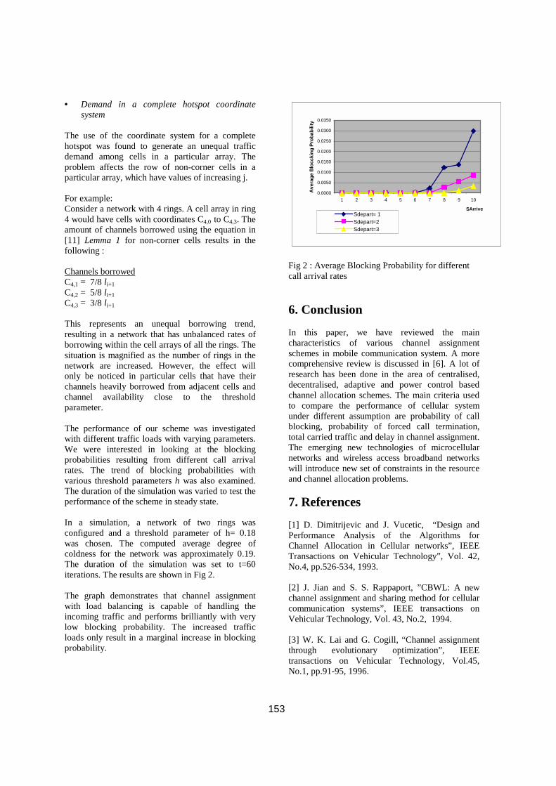
153

• Demand in a complete hotspot coordinate system

The use of the coordinate system for a complete hotspot was found to generate an unequal traffic demand among cells in a particular array. The problem affects the row of non-corner cells in a particular array, which have values of increasing j. For example: Consider a network with 4 rings. A cell array in ring 4 would have cells with coordinates C4,0 to C4,3. The amount of channels borrowed using the equation in [11] Lemma 1 for non-corner cells results in the following :

Channels borrowed C4,1 = 7/8 li+1 C4,2 = 5/8 li+1 C4,3 = 3/8 li+1

This represents an unequal borrowing trend, resulting in a network that has unbalanced rates of borrowing within the cell arrays of all the rings. The situation is magnified as the number of rings in the network are increased. However, the effect will only be noticed in particular cells that have their channels heavily borrowed from adjacent cells and channel availability close to the threshold parameter. The performance of our scheme was investigated with different traffic loads with varying parameters. We were interested in looking at the blocking probabilities resulting from different call arrival rates. The trend of blocking probabilities with various threshold parameters h was also examined. The duration of the simulation was varied to test the performance of the scheme in steady state. In a simulation, a network of two rings was configured and a threshold parameter of h= 0.18 was chosen. The computed average degree of coldness for the network was approximately 0.19. The duration of the simulation was set to t=60 iterations. The results are shown in Fig 2. The graph demonstrates that channel assignment with load balancing is capable of handling the incoming traffic and performs brilliantly with very low blocking probability. The increased traffic loads only result in a marginal increase in blocking probability.

0.0000

0.0050

0.0100

0.0150

0.0200

0.0250

0.0300

0.0350

1 2 3 4 5 6 7 8 9 10

SArrive

Ave

rage

Blo

ccki

ng P

roba

bilit

y

Sdepart= 1Sdepart=2Sdepart=3

Fig 2 : Average Blocking Probability for different call arrival rates 6. Conclusion In this paper, we have reviewed the main characteristics of various channel assignment schemes in mobile communication system. A more comprehensive review is discussed in [6]. A lot of research has been done in the area of centralised, decentralised, adaptive and power control based channel allocation schemes. The main criteria used to compare the performance of cellular system under different assumption are probability of call blocking, probability of forced call termination, total carried traffic and delay in channel assignment. The emerging new technologies of microcellular networks and wireless access broadband networks will introduce new set of constraints in the resource and channel allocation problems. 7. References [1] D. Dimitrijevic and J. Vucetic, “Design and Performance Analysis of the Algorithms for Channel Allocation in Cellular networks”, IEEE Transactions on Vehicular Technology”, Vol. 42, No.4, pp.526-534, 1993. [2] J. Jian and S. S. Rappaport, ”CBWL: A new channel assignment and sharing method for cellular communication systems”, IEEE transactions on Vehicular Technology, Vol. 43, No.2, 1994. [3] W. K. Lai and G. Cogill, “Channel assignment through evolutionary optimization”, IEEE transactions on Vehicular Technology, Vol.45, No.1, pp.91-95, 1996.

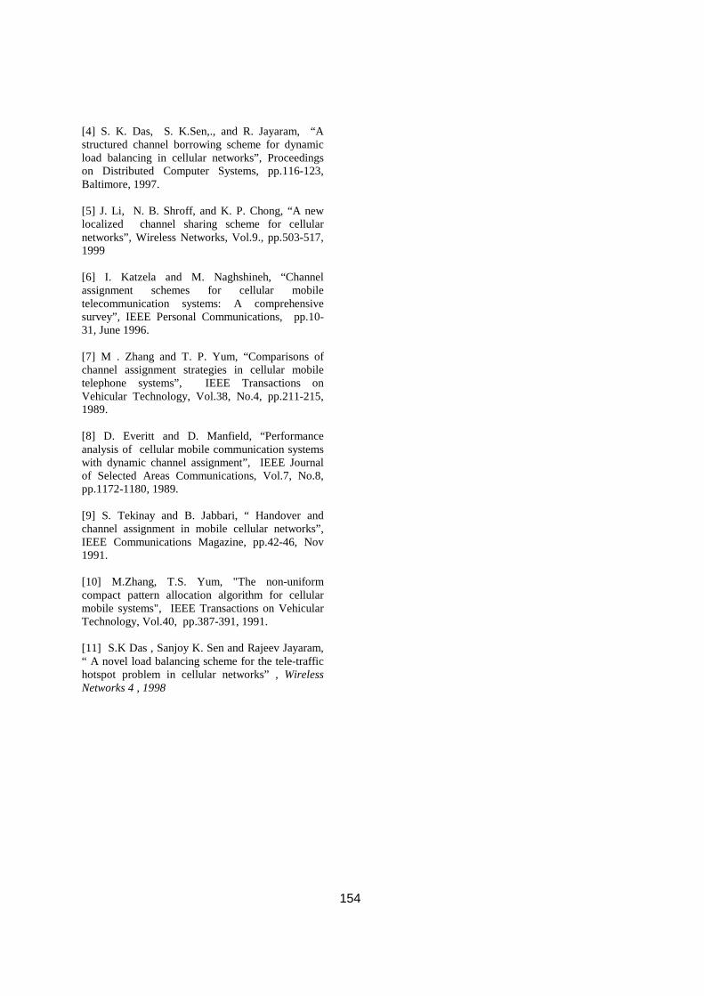
154

[4] S. K. Das, S. K.Sen,., and R. Jayaram, “A structured channel borrowing scheme for dynamic load balancing in cellular networks”, Proceedings on Distributed Computer Systems, pp.116-123, Baltimore, 1997. [5] J. Li, N. B. Shroff, and K. P. Chong, “A new localized channel sharing scheme for cellular networks”, Wireless Networks, Vol.9., pp.503-517, 1999 [6] I. Katzela and M. Naghshineh, “Channel assignment schemes for cellular mobile telecommunication systems: A comprehensive survey”, IEEE Personal Communications, pp.10-31, June 1996. [7] M . Zhang and T. P. Yum, “Comparisons of channel assignment strategies in cellular mobile telephone systems”, IEEE Transactions on Vehicular Technology, Vol.38, No.4, pp.211-215, 1989. [8] D. Everitt and D. Manfield, “Performance analysis of cellular mobile communication systems with dynamic channel assignment”, IEEE Journal of Selected Areas Communications, Vol.7, No.8, pp.1172-1180, 1989. [9] S. Tekinay and B. Jabbari, “ Handover and channel assignment in mobile cellular networks”, IEEE Communications Magazine, pp.42-46, Nov 1991. [10] M.Zhang, T.S. Yum, "The non-uniform compact pattern allocation algorithm for cellular mobile systems", IEEE Transactions on Vehicular Technology, Vol.40, pp.387-391, 1991. [11] S.K Das , Sanjoy K. Sen and Rajeev Jayaram, “ A novel load balancing scheme for the tele-traffic hotspot problem in cellular networks” , Wireless Networks 4 , 1998

155

A Concept of Differentiated Services Architecture Supporting Military Oriented Quality of Service

Marek Kwiatkowski

Defence Science and Technology Organisation (DSTO) PO Box 1500, Edinburgh, SA 5108, Australia

marek.kwiatkowski@dsto.defence.gov.au

Abstract This paper presents a concept of IP Differentiated Services (DiffServ) architecture in conjunction with bandwidth brokerage and policy based network management, all aimed at efficient and flexible provision of the Military oriented Quality of Service (M-QoS) features in the Australian Defence (strategic) Wide Area Network and its satellite trunk interconnections with the tactical domain. Typical DiffServ functions are analysed in the paper in regard to their roles in offering M-QoS. The paper proposes the use of bandwidth brokerage in each DiffServ domain to facilitate automatic Service Level Specification arrangements with end-user applications, and policy based network management to support the flexible implementation of bandwidth brokerage.

1. Introduction The term Military oriented Quality of Service (M-QoS), introduced in [5], represents commercial QoS in conjunction with the following features. Firstly, in military packet networks, when not enough network resources are available to support QoS for all traffic flows, the flows carrying mission critical information should get preference (i.e., higher priority) over less important flows. Secondly, in overloaded networks, it is preferable to gracefully "step down" the hard QoS1 of less important military flows instead of automatically tearing down these flows. Finally, higher flow priorities should be given for a restricted time defined by an enterprise policy.

IP Differentiated Services (DiffServ) is a promising new technology that could facilitate implementation of M-QoS in the Australian Defence strategic and tactical packet communication environment [6]. This is mainly because this technology is scalable, can provide both hard2 and soft QoS as well as graceful degradation in hard QoS to IP flows. However, DiffServ does not specify a standardised

1 Hard QoS offers an absolute reservation of resources for specific traffic, while soft QoS provides to some traffic a statistical preference over other traffic. 2 DiffServ can offer hard QoS through the use of an appropriate flow admission control and queueing mechanisms in routers.

User Network Interface to negotiate Service Level Specification in an automated fashion.

This paper presents a novel concept of IP DiffServ architecture in conjunction with bandwidth brokerage and policy based network management3, all aimed at efficient and flexible provision of the M-QoS features in an IP-oriented subset of the long-distance Australian Defence Core communication environment (further called Defence Core for short). This subset is composed of: (1) packet oriented strategic (terrestrial) networking infrastructure composed of the IP-based routing backbone network and the ATM-based Defence Corporate Backbone Network (DCBN); and (2) geo-synchronous earth orbit (GEO) satellite infrastructure used to: (a) interconnect the strategic network with tactical trunk networks; and (b) provide back-up connectivity for the strategic network.

It is stressed that currently the considered environment only offers best effort service. On the other hand, it is expected that the same environment will soon carry bulk Defence multimedia (i.e., voice, video and data) traffic of different importance. It is vital to provide the M-QoS features not only in bandwidth-impoverished parts of the Defence Core (such as satellite links), but also as broadly as possible. The reason for the latter is the need to maintain the ability to transmit mission critical information even if the environment is partially destroyed.

The paper is structured as follows. Section 2 presents a general concept of the proposed architecture. DiffServ functions, bandwidth brokerage and policy based network management supporting bandwidth brokerage are described in more detail in Sections 3, 4 and 5, respectively. Conclusions and future work are given in Section 6.

2. General Concept Following the analysis provided in [6], Figure 1 presents a combination of transmission technologies proposed to support M-QoS in the Defence Core. IPv4/IPv6 will generally be used for end-to-end

3 The term management refers here to longer time frame (e.g., hours, days) operations.

156

communication across the (terrestrial/satellite) Defence Core between end-user applications to transfer multimedia information. An open question is whether voice over IP (VoIP) can be carried over relatively slow satellite links. Note that DSTO is currently investigating this problem.

DiffServ will provide both hard and soft QoS as well as graceful degradation in hard QoS to IP flows. Both the strategic and tactical trunk networks will be divided into DiffServ domains. DiffServ will be augmented by the use of bandwidth brokerage. The latter will mainly be responsible for communication with end-user applications and flow admission control.

MPLS will be used to provide traffic engineering, mainly in the terrestrial part of the Defence Core. It seems to be desirable to use MPLS over a satellite to provide back-up links to the terrestrial Defence Core (see (a) in Figure 1), thus increasing its survivability. The use of MPLS between the strategic and tactical trunk domains (see (b) in Figure 1) requires further study.

ATM will still be used in DCBN, firstly to support MPLS switching, and secondly to continue carrying voice traffic until VoIP is implemented on a large scale. ATM may be required to transport voice over slow satellite links if IPv4/IPv6 and DiffServ do not satisfy the low jitter requirements.

Figure 2 presents the proposed DiffServ architecture in more detail. The Defence Core routing environment will be divided into a number of DiffServ domains. Routers in each domain

implement a number of Per-hop Behaviours (PHBs), each characterising the externally observable forwarding treatment applied at a DiffServ-compliant router to a collection of packets each having a distinct DiffServ Code Point (DSCP) value [2]. A maximum number of 64 PHBs can be created this way. Although, the parameters such as the number of PHBs, their characteristics and groupings will be decided in a relatively static fashion through an enterprise policy, we strongly suggest that packets representing different traffic types (e.g., file transfer, interactive, voice, video) and different military precedence levels (e.g., routine, flash) should belong to separate PHBs. This approach should facilitate dimensioning of network resources (e.g., buffers in routers) and flow admission control.

Each domain will be equipped with a single Bandwidth Broker (BB) entity. It will be responsible for automatic admitting to particular PHBs flows requiring (soft/hard) QoS and traversing the domain. To achieve this goal, the BB will communicate with:

• Local end-user applications (or their proxies) via a standard interface - to obtain information about parameters specifying the flows;

• Other BBs - to coordinate admission of flows that need to traverse a number of domains.

Note that BBs will not be involved in admitting best effort flows. In order to implement BB functions in a flexible and coordinated way amongst a number of BBs, Policy Administration will impose a single policy or a set of coherent policies onto BBs. It is assumed that these policies can often change, thus reflecting the dynamics of the battle space.

The next sections will present DiffServ functions, bandwidth brokerage and supporting it policy framework in more detail.

3. DiffServ Functions To implement a PHB, Defence Core routers will use typical DiffServ functions such as packet classification, marking, metering, policing (dropping), shaping and queueing [2]. Below, we present how these functions can support M-QoS features in a generic way. Since primarily Cisco routers are used in the considered Defence Core environment, we will also discuss how these functions can be implememented using Cisco routers. It is noted that DSTO is currently conducting experiments with various configuration arrangements of DiffServ functions in Cisco routers.

M-QoS oriented Network Control and Mgnt

Bandwidth Brokerage

Tactical DiffServ domain Strategic

DiffServ domain IPv4/IPv6 DiffServ

MPLS ATM ATM (?)

MPLS (?)

Figure 1. General concept data network cntrl & mgnt

host host

(a)

157

3.1 Packet Classification Packets entering a router will be classified to one of the specified PHBs using filters. Our concept assumes that packets sent from end-user applications to ingress routers (IRs) will be classified based on the 5-tuple (source IP address, source port number, destination IP address, destination port number, and the transport protocol). The rules for classifying a flow in IRs will be delivered by the domain’s Bandwidth Broker after deciding to admit the flow. All other (transit/egress/boundary) routers will have statically configured filters, which will classify packets based on their DSCP value set during packet marking (see below) in IRs. We propose the use of Access Lists [3] to implement packet classification in Cisco routers.

3.2 Packet Metering Packet metering is used to measure temporal properties of a flow (flow aggregates) selected by the classifier against a traffic profile specified in a Service Level Specification (SLS) and/or against any relevant policy requirements. In our concept, packet metering will be required when implementing policing, shaping and queueing functions.

As for Cisco routers, packet metering is in-built in the latter functions.

3.3 Packet Marking Packet marking is the process of setting the DSCP value in a packet based on defined rules. In our approach, packets are marked by IRs based on results of packet classification and metering. The rules for marking are specified by BBs at the time of admitting flows.

As for Cisco routers, marking will be implemented as a part of the policing mechanism (see below).

3.4 Packet Policing This process aims at discarding packets based on information provided by meters, and according to the rules specified by BBs.

In our concept, policing in IRs will be applied to all (military-essential) flows admitted by BBs. BBs will be responsible for sending to the routers a specification of dropping rules. This policing will be crucial to assure conformance of end-user application traffic to the previously negotiated SLS. It is stressed that individual best-effort flows will not be policed.

We propose the use of Two Rate Three Color Marker [4] to carry out packet dropping. In Cisco routers it can be implemented by Two-Rate Policer, which, as indicated above, also covers packet metering and packet marking.

Host

Milsatcom Strategic Environment Tactical Environment

Host

BB

M-QoS interface

Strat. DiffServ Domain

Policy Administration

Tactical DiffServ Domain

Strat. DiffServDomain

BB

M-QoS interface

BB

QoS mgnt Inter-BB sign.

User data

Router

QoS control

Figure 2. Proposed concept of DiffServ architecture

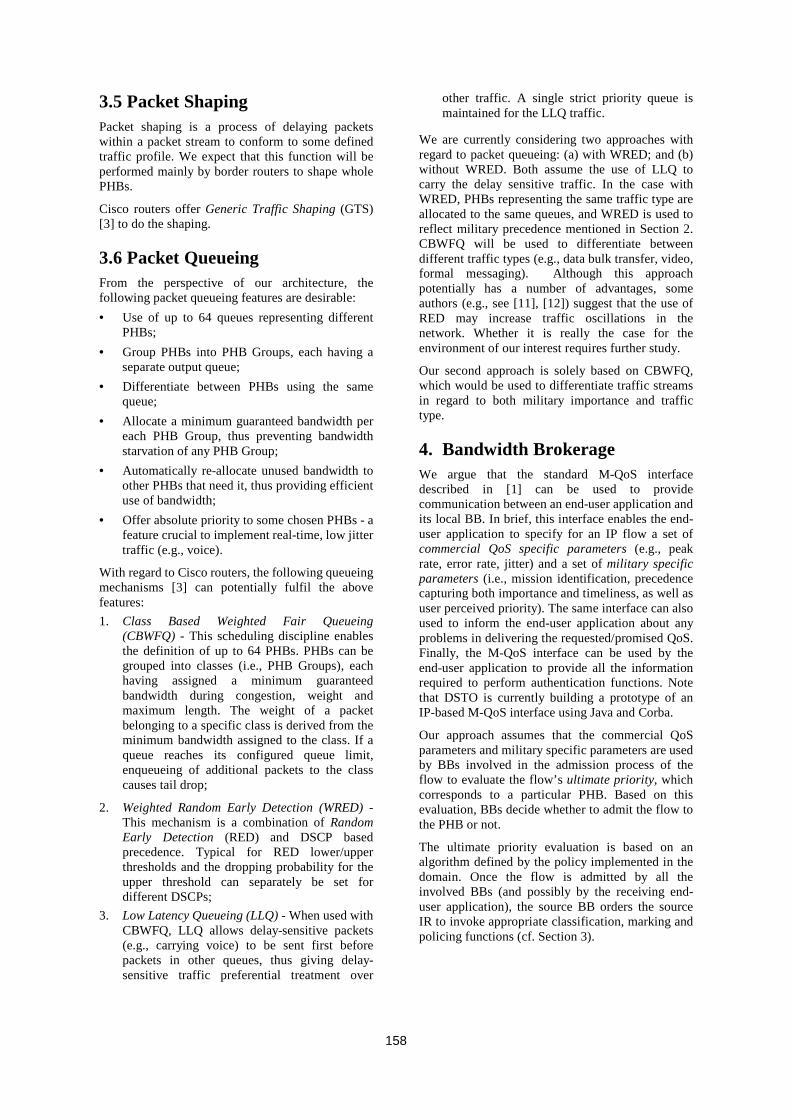
158

3.5 Packet Shaping Packet shaping is a process of delaying packets within a packet stream to conform to some defined traffic profile. We expect that this function will be performed mainly by border routers to shape whole PHBs.

Cisco routers offer Generic Traffic Shaping (GTS) [3] to do the shaping.

3.6 Packet Queueing From the perspective of our architecture, the following packet queueing features are desirable: • Use of up to 64 queues representing different

PHBs; • Group PHBs into PHB Groups, each having a

separate output queue; • Differentiate between PHBs using the same

queue; • Allocate a minimum guaranteed bandwidth per

each PHB Group, thus preventing bandwidth starvation of any PHB Group;

• Automatically re-allocate unused bandwidth to other PHBs that need it, thus providing efficient use of bandwidth;

• Offer absolute priority to some chosen PHBs - a feature crucial to implement real-time, low jitter traffic (e.g., voice).

With regard to Cisco routers, the following queueing mechanisms [3] can potentially fulfil the above features: 1. Class Based Weighted Fair Queueing

(CBWFQ) - This scheduling discipline enables the definition of up to 64 PHBs. PHBs can be grouped into classes (i.e., PHB Groups), each having assigned a minimum guaranteed bandwidth during congestion, weight and maximum length. The weight of a packet belonging to a specific class is derived from the minimum bandwidth assigned to the class. If a queue reaches its configured queue limit, enqueueing of additional packets to the class causes tail drop;

2. Weighted Random Early Detection (WRED) - This mechanism is a combination of Random Early Detection (RED) and DSCP based precedence. Typical for RED lower/upper thresholds and the dropping probability for the upper threshold can separately be set for different DSCPs;

3. Low Latency Queueing (LLQ) - When used with CBWFQ, LLQ allows delay-sensitive packets (e.g., carrying voice) to be sent first before packets in other queues, thus giving delay-sensitive traffic preferential treatment over

other traffic. A single strict priority queue is maintained for the LLQ traffic.

We are currently considering two approaches with regard to packet queueing: (a) with WRED; and (b) without WRED. Both assume the use of LLQ to carry the delay sensitive traffic. In the case with WRED, PHBs representing the same traffic type are allocated to the same queues, and WRED is used to reflect military precedence mentioned in Section 2. CBWFQ will be used to differentiate between different traffic types (e.g., data bulk transfer, video, formal messaging). Although this approach potentially has a number of advantages, some authors (e.g., see [11], [12]) suggest that the use of RED may increase traffic oscillations in the network. Whether it is really the case for the environment of our interest requires further study.

Our second approach is solely based on CBWFQ, which would be used to differentiate traffic streams in regard to both military importance and traffic type.

4. Bandwidth Brokerage We argue that the standard M-QoS interface described in [1] can be used to provide communication between an end-user application and its local BB. In brief, this interface enables the end-user application to specify for an IP flow a set of commercial QoS specific parameters (e.g., peak rate, error rate, jitter) and a set of military specific parameters (i.e., mission identification, precedence capturing both importance and timeliness, as well as user perceived priority). The same interface can also used to inform the end-user application about any problems in delivering the requested/promised QoS. Finally, the M-QoS interface can be used by the end-user application to provide all the information required to perform authentication functions. Note that DSTO is currently building a prototype of an IP-based M-QoS interface using Java and Corba.

Our approach assumes that the commercial QoS parameters and military specific parameters are used by BBs involved in the admission process of the flow to evaluate the flow’s ultimate priority, which corresponds to a particular PHB. Based on this evaluation, BBs decide whether to admit the flow to the PHB or not.

The ultimate priority evaluation is based on an algorithm defined by the policy implemented in the domain. Once the flow is admitted by all the involved BBs (and possibly by the receiving end-user application), the source BB orders the source IR to invoke appropriate classification, marking and policing functions (cf. Section 3).

159

It is stressed that in our approach, admission of a flow may result in degradation of other, less important flows, thus reflecting the idea of graceful degradation of QoS. This may also apply to hard QoS flows. For example, a flow carrying voice with precedence level flash can partially or completely preempt another voice flow having precedence level routine.

Other expected BB functions include: • Evaluation of time restrictions related to the

military precedence level of a flow. Such restrictions may trigger a change in the flow’s classification (e.g., from flash to routine) at the flow’s IR;

• Modification (if required) of reservations for pending flows;

• Organising monitoring of domain’s resources and tracking SLSs of active flows.

Some form of inter BB communication is necessary to perform the above functions for cross-domain flows (cf. Figure 2). We propose to base this communication on the Simple Interdomain Bandwidth Broker Signalling (SIBBS) protocol being finalised within the QBone Project [8,10]. Note that DSTO is currently investigating the ability of this protocol to fully support the M-QoS requirements.

5. Policy Framework The proposed approach to policy-based M-QoS management is based on the IETF policy framework [7], and comprises the following generic components: a. Policy Administration (PA) – responsible for

consistent DiffServ offerings across all Defence Core domains. It controls multiple BBs, automatically distributes changes to the policy, and correlates feedback from BBs regarding the

health of their domains. Policy Administration retrieves policies from a policy repository(ies);

b. Bandwidth Broker/Policy Decision Point (BB/PDP) – plays a dual role, firstly acting as a PDP in relation to Policy Administration, and secondly performing typical Bandwidth Broker functionality;

c. Other Policy Servers – examples of such servers include an authentication server(s) and an accounting server(s);

d. Policy Enforcement Points – these are mainly DiffServ-enabled routers capable of enforcing QoS policy rules.

As depicted in Figure 2, policy administration needs to cover both strategic and tactical DiffServ domains to provide end-to-end M-QoS. A complete centralisation of this administration in the strategic environment may not be desirable since a substantial amount of policy information may refer to these BB functions, which are strictly related to tactical domains operating in isolation. In such a case, sending to these domains all the policy details from a single strategic repository via relatively low bandwidth and unreliable satellite links may create performance and reliability issues. Therefore, it seems to be beneficial to distribute policy management. There are a number of possible approaches to such distribution. A plausible one is presented in Figure 3, where a single strategic policy administrator (S-PA) controls all fixed DiffServ domains using a policy stored on its strategic policy repository (S-PR). In addition, each tactical DiffServ domain has its own PA (depicted as T-PA in Figure 3) responsible for M-QoS delivery within the domain according to a policy stored on the tactical policy repository (T-PR). To achieve consistent M-QoS across strategic/tactical domains, all policies have to be coordinated using communication between S-PA and T-PAs across satellite links (see Figure 3).

MilsatcomStrategic Environment Tactical Environment

BB/PDP

S-PA S-PR

T-PR

T-PA

BB/PDP BB/PDP BB/PDP

T-PR

T-PA

BB/PDP

Policy coordination

Policy distribution DiffServ domain

Figure 3. Considered approach to policy distribution/coordination supporting bandwidth brokerage

160

6. Conclusions and Further Work In this paper we have proposed a flexible and scalable solution to implement M-QoS within the Australian Defence terrestrial/satellite Defence Core using Differentiated Services (DiffServ) in conjunction with bandwidth brokerage and supporting it policy-based network management.

A number of issues require further investigation, including: • Design of viable flow admission control

algorithm(s) and performance monitoring; • Setting of CBWFQ and WRED parameters to

achieve a particular PHB differentiation; • Performance aspects (e.g., consumed

bandwidth) related to inter-domain brokerage signalling over slow satellite trunks;

• Efficient and reliable distribution of policy administration for dispersed strategic/tactical trunk communications involving satellite communication.

Note that DSTO is currently investigating the first two groups of issues. It is also noted that DSTO is conducting research under the aegis of The Technical Cooperation Program (TTCP) [9] on the applicability of the proposed DiffServ architecture to a coalition environment.

References [1] P. Blackmore, P. George, M. Kwiatkowski “A

Quality of Service Interface for Military Applications”, IEEE MILCOM’00 Conference, Los Angeles, Oct. 2000.

[2] S. Blake et al, “An Architecture for Differentiated Services”, IETF RFC 2475, Dec. 1998.

[3] Cisco IOS Release 12.2, 2001.

[4] Heinanen et al, “A Two Rate Three Color Marker”, RFC 2968, Sept. 98.

[5] M. Kwiatkowski, P. George, “A Network Control and Management Framework Supporting Military Quality of Service”, IEEE MILCOM’99 Conference, Atlantic City, USA, Oct. 1999.

[6] M. Kwiatkowski, “An Assessment of Commercial Transmission Technologies to Support Military Oriented Quality of Service”, (unclassified) DSTO Technical Report, Oct. 2001.

[7] IETF, Policy Charter, http://www.ietf.org/html.charters/policy-charter.html

[8] B. Teitelbaum et al, “Internet2 Qbone: Building a Testbed for Differentiated Services”, IEEE Communications Magazine, Sept./Oct. 1999.

[9] The Technical Cooperation Program (TTCP), http://www.dtic.mil/ttcp/

[10] QBone Signaling Design Team http://qbone.internet2.edu/bb/index.shtml

[11] Th. Bonald, M. May, J. Bolot, “Analytic Evaluation of RED Performance”, IEEE INFOCOM’00 Conference.

[12] S.H. Low et al, “Dynamics of TCP/RED and a Scalable Control”, IEEE INFOCOM’02 Conference, New York, June 2002.

A SCALABLE TO LOSSLESS AUDIO COMPRESSION SCHEME

Mohammed Raad, Alfred Mertins and Ian Burnett

School of Electrical, Computer and Telecommunications Engineering

University Of Wollongong

Northelds Ave Wollongong NSW 2522 Australia

email: mr10@uow.edu.au

ABSTRACT

This paper outlines a scalable to lossless coder, that is the coderpresented is a scalable coder that scales from lossy quality tolossless quality. Lossless compression is achieved by concate-nating a lossy, scalable transform coder with a scalable schemefor the compression of the synthesis error signal. The losslesscompression results obtained are comparable with the state ofthe art in lossless compression (that is a compression ratio rang-ing from 1.74 to 5.27). The added advantage of the compres-sion scheme presented is the scalability, which is obtained bybasing the lossy coder on the Set Partitioning In HierarchicalTrees (SPIHT) algorithm.

1. INTRODUCTION

With the introduction of third generation cellular phone sys-tems and the possible expansion of those systems, digital cellu-lar phone users may in the near future have access to data ratesabove 144 kbps [1]. This is a considerable increase on whatthe second generation of mobile telephony presented, knownas GSM [1, 2], which in most implementations only providesusers access to 9.6 kbps of data [1]. Such an explosion inthe possible bit rate and the nature of the proposed bit streamsmeans that multimedia compression schemes may be adjustedto allow for increased quality of the delivered product to theuser. The other well known medium of multimedia delivery,the internet, is also experiencing an increase in possibilitieswith the introduction of broadband technology.

The increase in bit rates means that audio compression al-gorithms with higher bit rates than currently used, such as MPEG’smp3 [3], can be used to obtain higher quality. However, thenew increased data rates are not necessarily constant. This isespecially the case when considering the internet. As such,scalable and lossless schemes have become rather interestingfrom an application point of view.

Currently, lossless audio coding has been approached froma signal model perspective [4],[5],[6]. The signal is typicallymodelled using a linear predictor, which may either be FIR oras in the case of [5] IIR. The compression ratio of such coders

typically depends on the nature of the audio signal being codedand may range between 1.4 and 5.3 [4].

Similarly, scalable audio compression has been approachedfrom a signal model point of view. Recent scalable codingschemes, such as the scheme described in [7], use a compositesignal model. The model is built through the combination ofSinusoids, Transients and Noise (STN). The STN model of anaudio signal is described in detail in [7] and [8]. The scalabilityobtained in [7] is mainly large step scalability, with more gran-ular scalability made possible through the use of an adequatelydesigned entropy code. The system in [7] is scalable between 6kbps and 80 kbps, however as different frame lengths are usedto model the different signal components more adequately thescheme is presented more as an ‘off-line’ tool in [7].

With the aim of standardizing a scalable compression scheme,MPEG proposed different audio coders for different rates [3].A scalable parametric coder has been adopted by MPEG as de-scribed in [9], which is built around a sinusoidal model of theaudio signal.

Having described the advances in the bandwidth availabil-ity for cellular telephones, and that for internet users, it is clearthat a compression scheme that combines both scalability andlossless compression is of interest and potential use. MPEGhave started a process of standardization for such a scheme[10].

In this paper we present an implementation of a scalableaudio coder that allows very fine granular scalability as wellas compression at the lossless stage. The compression schemeis built around transform coding of audio. Particularly, the SetPartitioning In Hierarchical Trees (SPIHT) algorithm [11] isused to allow scalability as well as perfect reconstruction. Theresults presented show that significant lossless compression isobtained.

2. LOSSLESS AUDIO COMPRESSION

Lossless compression of audio aims to reduce the bandwidth ormemory required to transmit or store the original audio signal.That is, the error between the original Pulse Code Modulated(PCM) signal and the compressed version is zero. The major-

Input Audio (PCM)

Predictor

(Quantized)

Entropy Coder-

Figure 1: Lossless Compression using Linear Prediction

Input Audio

T Q -1T PCMQ

-

Transform Coefficients

Error (entropy coded)

Figure 2: Lossless Compression Using Transform Cod-ing

ity of digital audio material in use today is quantized using 16bits per sample and obtained at a sampling frequency of 44.1kHz. That is the CD standard of a digital audio signal, howeverother sampling rates may be used and a different quantizationscheme utilized.

A lossless compression scheme achieves the stated aim bythe removal of redundancy in the original signal. This redun-dancy is typically removed by the use of a linear predictor [4].The output of the linear predictor is treated as the approxima-tion of the audio signal. The error between the original signaland the approximate signal is typically coded through the useof an entropy code, such as Huffman or Rice, which are loss-less. Figure 1 illustrates a typical lossless scheme.

Lossless audio compression may be viewed as an adapta-tion of more general lossless coding schemes such as ‘LempelZiv’ [12] which attempt to reduce the storage capacity requiredfor a given set of samples. However, it has been found that suchalgorithms only produce a small amount of compression whenapplied to PCM audio signals [6], and hence the use of algo-rithms that take advantage of the nature of the audio signal. Thelinear prediction algorithms tend to use frame lengths of ap-proximately 25 ms to take advantage of the pseudo-stationarynature of the audio signal of that length.

It has been argued in [13] that transform coding would bemore suitable for lossless compression as it models the audiosignal more accurately. Lossy audio compression is fundamen-tally based on transform coding [14] as that allows the har-monic nature of the audio signal to be captured. Based on thismodel, the work in [13] proposes approximating the audio sig-nal by the use of a transform coder and coding the error signalby the use of an entropy code. Figure 2 shows the structure ofthe lossless coder proposed in [13]. This approach is actuallyvery similar in nature to the linear prediction approach as theuse of the transform coder decorrelates the audio samples andhence the transform coder operates on the same basic princi-

ples of decorrelation and entropy coding as the linear predic-tion based lossless coders [4]. The compression ratios reportedin [13] again varied with the nature of the input audio signaland ranged between 2.2 and 3.2 for the test set that was used,which had some similarity with that presented in [4] but wasnot exactly the same.

The vast majority of lossless compression algorithms canbe grouped under the two groups of prediction based codersand transform based coders as described previously [4], [13],[10]. However, such coders have been optimized to obtainthe greatest possible compression at lossless operation. Also,all the coders reviewed here are variable rate coders. Hav-ing an optimized lossless scheme limits the ability to use sucha scheme in a scalable system. Similarly, a scalable systemshould be theoretically scalable to lossless with a preferablylinear increase in perceptual quality. In the next section wepresent a scalable to lossless scheme that allows bit rates to becontrolled bitwise. That is, each bit received adds to the qualityof the synthesized signal, in terms of signal to noise ratio.

3. A SCALABLE TO LOSSLESS SCHEME

USING SPIHT

To achieve lossless compression, that is to obtain zero error be-tween the original signal and the synthesized signal, a numberof approaches may be taken. Section 2 discussed the currentapproaches taken by researchers. Building on the approach of[13], a lossy transform compression scheme may be combinedwith a lossless compression scheme for the error signal. In ourcase, the lossy transform scheme is actually a scalable scheme.In a previous work involving SPIHT [15] we presented resultsthat indicated the developed coder produced very good syn-thesized audio (that is, near perceptually insignificant error) atrates around and above 56 kbps. That coder used the MLT, aswell as a perceptual model that removed perceptually insignif-icant signal components.

The solution proposed here is also built on that system of[15] but without the perceptual model. Figure 3 shows the pro-posed coder The input signal is transformed using the MLT,here floating point calculations are used, the signal is coded us-ing SPIHT and the bit-stream transmitted to the decoder. Wewill refer to the first bit stream as bit stream one. Bit streamone is decoded at the encoder and the synthesized audio is sub-tracted from the original audio to obtain the output error. Hereinteger operations are used so that the error output is integer,and typically has a dynamic range that is equal to or less thanthat of the original integer signal (otherwise the lossy compres-sion scheme would not have done a good job of mimickingthe original signal). An Example of the difference in dynamicrange between the original audio signal and the synthesizedsignal is shown in Figure 4 where the original signal is codedat 64 kbps. The smaller dynamic range is important when cod-ing a signal with losslessly (see the discussion in [16]). In the

present case, the given coefficients are in the time domain. Al-though SPIHT was originally aimed at frequency domain sig-nals [11], the error signal has an important property in commonwith a frequency domain signal (that is one transformed fromthe time domain) in that its individual samples are much lesscorrelated with each other than the original samples. In factthe more bits that are spent on the compression of the originalsignal the more white-noise like is the error signal. To illustratethis, Figure 5 shows the PSD of two versions of the error signalfor a coded frame of audio at rates of 64 kbps and 128 kbps.

Hence, the shrinking of the dynamic range improves thecoding performance of SPIHT for the error signal, and the un-correlated nature of the time domain error signal means thatvery little will be gained if the signal is transformed, and so inthis case it is not.

Having developed the idea to this stage, it is now impor-tant to decide the rate to which the lossy side of the coderoperates. The accuracy of the synthesized signal to the orig-inal is dictated by the quantization resolution that is chosen inSPIHT. Quantization resolution in this context refers to the res-olution chosen to quantize the frequency domain transform co-efficients, and should not be confused with the resolution usedfor the quantization of the time domain signal, which is 16 bitsPCM. Figure 6 shows the relationship between the SegSNRand the quantization resolution used in SPIHT (here completereconstruction of the quantized transform coefficients is used).The 13 SQAM files (Cd quality, monotone) used in obtainingthe results discussed in this paper are listed in Table 1. Thecurves in the figure are quite linear indicating a linear trade-offbetween synthesized signal quality and quantization resolution(remember that in this case no perceptual model is being used).As a matter of experience, a SegSNR of 50 dB produces verygood quality and so the quantization resolution that is used inthe first section of the coder has been set to 18 bits, as all of thecoded files show a SegSNR well above 50 dB at that quantiza-tion resolution.

The combination of bit stream one and bit stream two givesthe complete bit stream which determines the rate of the coder.The base rate which produces the least overall rate may be de-termined experimentally, Table 2 shows the results of an exper-iment with a voiced section of signal x1. The table includes thefirst order entropy of the error signal, obtained with the equa-tion:

H(x) = X

x2X

p(x) log2p(x) (1)

The first order entropy indicates the expected limit to loss-lessly code the error bit stream. Using this expected limit, theexpected lowest rate is calculated. Table 2 shows that the low-est expected rate is obtained when a base rate of 192 kbps isused. This does not match the actual rate results exactly (thefinal column in the table), yet it is close. The difference be-tween the expected overall rate and the actual is due to the sort-ing carried out by SPIHT. The entropy describes the minimum

Normalize

(Floating Point)

MLT

SPIHT Encode

Bit Stream OneBit Stream Two

SPIHT Encode

SPIHT Decode

SPIHT Decode SPIHT Decode

PCMQ

Input Audio (PCM)

Output Audio (PCM)

-

PCMQ

Inv MLT

Figure 3: The Scalable to Lossless scheme based onSPIHT

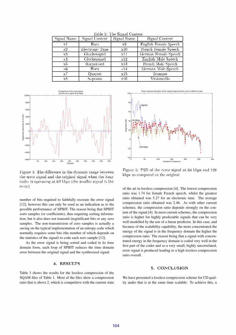
Table 1: The Signal ContentSignal Name Signal Content Signal Name Signal Content

x1 Bass x9 English Female Speech

x2 Electronic Tune x10 French Female Speech

x3 Glockenspiel x11 German Female Speech

x4 Glockenspiel x12 English Male Speech

x5 Harpsicord x13 French Male Speechx6 Horn x14 German Male Speech

x7 Quartet x15 Trumpet

x8 Soprano x16 Violoncello

50 100 150 200 250 300 350 400 450 500−8000

−6000

−4000

−2000

0

2000

4000

6000

8000

10000

Samples

Mag

nitu

de (

quan

tized

at 1

6 bi

ts)

Comparison of the input signal and the error signal at 64 kbps

Figure 4: The dierence in the dynamic range betweenthe error signal and the original signal when the lossycoder is operating at 64 kbps (the smaller signal is theerror)

number of bits required to faithfully recreate the error signal[12], however this can only be used as an indication as to thepossible performance of SPIHT. The reason being that SPIHTsorts samples (or coefficients), thus requiring sorting informa-tion, but it also does not transmit insginificant bits or any zerosamples. The non-transmission of zero samples is actually asaving on the typical implementation of an entropy code whichnormally requires some bits (the number of which depends onthe statistics of the signal) to code each zero sample [12].

As the error signal is being sorted and coded in its timedomain form, each loop of SPIHT reduces the time domainerror between the original signal and the synthesized signal.

4. RESULTS

Table 3 shows the results for the lossless compression of theSQAM files of Table 1. Most of the files show a compressionratio that is above 2, which is competitive with the current state

0 50 100 150 200 250 300−40

−20

0

20

40

60

80

100

Samples in frequency

Mag

nitu

de (

dB)

Power Spectral densities of the original signal and the error at different rates

64 kbps

original

128 kbps

Figure 5: PSD of the error signal at 64 kbps and 128kbps as compared to the original

of the art in lossless compression [4]. The lowest compressionratio was 1.74 for female French speech, whilst the greatestratio obtained was 5.27 for an electronic tune. The averagecompression ratio obtained was 2.46. As with other currentschemes, the compression ratio depends strongly on the con-tent of the signal [4]. In most current schemes, the compressionratio is higher for highly predictable signals that can be verywell modelled by the use of a linear predictor. In this case, andbecause of the scalability capability, the more concentrated theenergy of the signal is in the frequency domain the higher thecompression ratio. The reason being that a signal with concen-trated energy in the frequency domain is coded very well in thefirst part of the coder and so a very small, highly uncorrelated,error signal is produced leading to a high lossless compressionratio overall.

5. CONCLUSION

We have presented a lossless compression scheme for CD qual-ity audio that is at the same time scalable. To achieve this, a

Table 2: Experimental Results for The Overall Rate Given Various Base RatesBase Rate First Order Entropy Total Rate Expected Actual Error Rate Actual Total Rate(kbps) (bits per sample) (kbps) (kbps) (kbps)

64 7.02 374 344 40880 6.48 366 329 40996 6.01 362 305 401128 5.24 359 273 401192 3.72 356 213 405256 2.56 369 170 426

10 12 14 16 18 20 22 2410

20

30

40

50

60

70

80

90

100

110

Quantization level (n)

Seg

SN

R (

dB)

SegSNR vs quantization level for 13 of the SQAM files

x1 x2 x3 x4 x5 x6 x7 x9 x11x13x14x15x16

Figure 6: The SegSNR vs the quantization resolutionfor the lossy side of the coder

scalable lossy scheme has been combined with a scalable timedomain scheme. Both schemes are built around SPIHT, andthe combination of these two schemes has produced losslesscompression results that are comparable with the current stateof the art. The results presented are mean bit rates, howeverthe coder does have the added advantage of having its bit ratecontrolled to a resolution of one bit.

6. ACKNOWLEDGEMENT

Mohammed Raad is in receipt of an Australian PostgraduateAward (industry) and a Motorola (Australia) Partnerships inResearch Grant.

7. REFERENCES

[1] K.W. Richardson, “UMTS overview,” Electronics andcommunication engineering journal, vol. 12, no. 3,pp. 93–100, June 2000.

[2] Jorg Eberspacher and Hans-Jorg Vogel, GSM Switch-

Table 3: Results for The Lossless SPIHT CoderSignal Rate Compression Ratio Bits/Sample

(kbps)

x1 318 2.22 7.20x2 134 5.27 3.03x3 206 3.43 4.65x4 266 2.65 6.01x5 346 2.04 7.84x6 232 3.04 5.23x7 354 1.99 8.01x8 317 2.23 7.18x9 366 1.93 8.28x10 405 1.74 9.17x11 362 1.95 8.19x12 368 1.92 8.33x13 360 1.96 8.15x14 360 1.96 8.15x15 255 2.77 5.75x16 306 2.31 6.93

ing, Services and Protocols, John Wiley and Sons,Chichester, 1999.

[3] K Brandenburg, O Kunz, and A Sugiyama, “MPEG-4 natural audio coding,” Signal Processing: Image

Communication, vol. 15, no. 4, pp. 423–444, Jan. 2000.

[4] M. Hans and R.W. Schafer, “Lossless compression ofdigital audio,” IEEE Signal Processing magazine,vol. 18, no. 4, pp. 21–32, July 2001.

[5] P.G. Craven and M.J. Law, “Lossless compression us-ing IIR prediction filters,” AES 102nd convention, AESpreprint 4415, March 1997.

[6] A.A.M.L. Bruekers, W.J. Oomen, and R.J. van derVleuten, “Lossless coding for DVD audio,” AES 101stconvention, AES preprint 4358, November 1996.

[7] T.S. Verma, A perceptually based audio signal model

with application to scalable audio compression,Ph.D. thesis, Department of Electrical Engineering, Stan-ford university, October 1999.

[8] S.N. Levine, Audio representations for data com-

pression and compressed domain processing, Ph.D.thesis, Department of electrical engineering, Stanforduniversity, December 1998.

[9] H. Purnhagen and N. Miene, “HILN - the MPEG-4parametric audio coding tools,” in Proceedings of IS-

CAS 2000, 2000, vol. 3, pp. 201–204.

[10] T. Moriya, “Report of AHG on issues in lossless au-dio coding,” ISO/IEC JTC1/SC29/WG11 M7955, March2002.

[11] Amir Said and William A. Pearlman, “A new, fast, andefficient image codec based on set partitioning in hier-archical trees,” IEEE Transactions on Circuits and

Systems For Video Technology, vol. 6, no. 3, pp. 243–250, June 1996.

[12] S.W. Golomb, R.E. Peile, and R.A. Scholtz, Basic Con-

cepts in Information Theory and Coding, Plenumpress, NY, 1994.

[13] T. Liebchen, M. Purat, and P. Noll, “Lossless transformcoding of audio signals,” Proceedings of the 102nd

AES convention, AES preprint 4414, March 1997.

[14] Peter Noll, “MPEG digital audio coding,” IEEE Sig-

nal Processing Magazine, vol. 14, no. 5, pp. 59–81,Sept. 1997.

[15] M. Raad, A. Mertins, and I. Burnett, “Audio compres-sion using the MLT and SPIHT,” Proceedings of

DSPCS' 02, pp. 128–132, 2002.

[16] C.D. Giurcaneanu, I. Tabus, and J. Astola, “Adap-tive context-based sequential prediction for lossless au-dio compression,” Signal Processing, vol. 80, no. 11,pp. 2283–2294, November 2000.

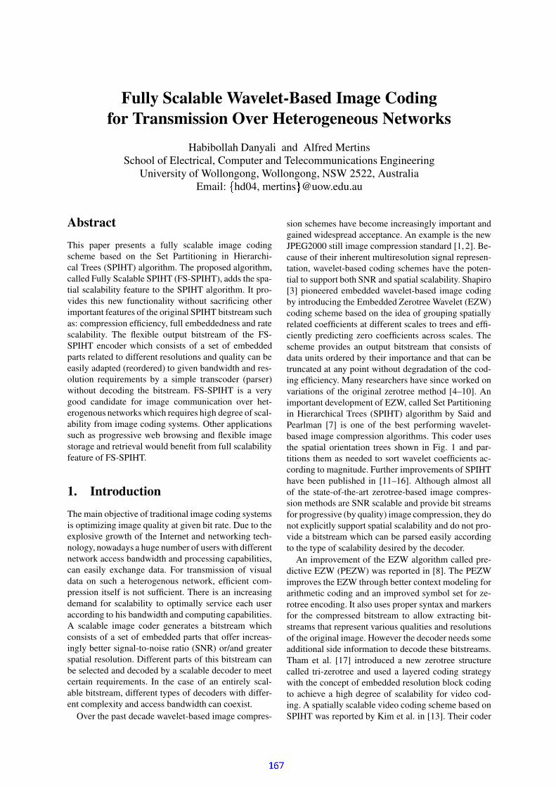
Fully Scalable Wavelet-Based Image Codingfor Transmission Over Heterogeneous Networks

Habibollah Danyali and Alfred MertinsSchool of Electrical, Computer and Telecommunications Engineering

University of Wollongong, Wollongong, NSW 2522, AustraliaEmail:

hd04, mertins @uow.edu.au

Abstract

This paper presents a fully scalable image codingscheme based on the Set Partitioning in Hierarchi-cal Trees (SPIHT) algorithm. The proposed algorithm,called Fully Scalable SPIHT (FS-SPIHT), adds the spa-tial scalability feature to the SPIHT algorithm. It pro-vides this new functionality without sacrificing otherimportant features of the original SPIHT bitstream suchas: compression efficiency, full embeddedness and ratescalability. The flexible output bitstream of the FS-SPIHT encoder which consists of a set of embeddedparts related to different resolutions and quality can beeasily adapted (reordered) to given bandwidth and res-olution requirements by a simple transcoder (parser)without decoding the bitstream. FS-SPIHT is a verygood candidate for image communication over het-erogenous networks which requires high degree of scal-ability from image coding systems. Other applicationssuch as progressive web browsing and flexible imagestorage and retrieval would benefit from full scalabilityfeature of FS-SPIHT.

1. Introduction

The main objective of traditional image coding systemsis optimizing image quality at given bit rate. Due to theexplosive growth of the Internet and networking tech-nology, nowadays a huge number of users with differentnetwork access bandwidth and processing capabilities,can easily exchange data. For transmission of visualdata on such a heterogenous network, efficient com-pression itself is not sufficient. There is an increasingdemand for scalability to optimally service each useraccording to his bandwidth and computing capabilities.A scalable image coder generates a bitstream whichconsists of a set of embedded parts that offer increas-ingly better signal-to-noise ratio (SNR) or/and greaterspatial resolution. Different parts of this bitstream canbe selected and decoded by a scalable decoder to meetcertain requirements. In the case of an entirely scal-able bitstream, different types of decoders with differ-ent complexity and access bandwidth can coexist.

Over the past decade wavelet-based image compres-

sion schemes have become increasingly important andgained widespread acceptance. An example is the newJPEG2000 still image compression standard [1, 2]. Be-cause of their inherent multiresolution signal represen-tation, wavelet-based coding schemes have the poten-tial to support both SNR and spatial scalability. Shapiro[3] pioneered embedded wavelet-based image codingby introducing the Embedded Zerotree Wavelet (EZW)coding scheme based on the idea of grouping spatiallyrelated coefficients at different scales to trees and effi-ciently predicting zero coefficients across scales. Thescheme provides an output bitstream that consists ofdata units ordered by their importance and that can betruncated at any point without degradation of the cod-ing efficiency. Many researchers have since worked onvariations of the original zerotree method [4–10]. Animportant development of EZW, called Set Partitioningin Hierarchical Trees (SPIHT) algorithm by Said andPearlman [7] is one of the best performing wavelet-based image compression algorithms. This coder usesthe spatial orientation trees shown in Fig. 1 and par-titions them as needed to sort wavelet coefficients ac-cording to magnitude. Further improvements of SPIHThave been published in [11–16]. Although almost allof the state-of-the-art zerotree-based image compres-sion methods are SNR scalable and provide bit streamsfor progressive (by quality) image compression, they donot explicitly support spatial scalability and do not pro-vide a bitstream which can be parsed easily accordingto the type of scalability desired by the decoder.

An improvement of the EZW algorithm called pre-dictive EZW (PEZW) was reported in [8]. The PEZWimproves the EZW through better context modeling forarithmetic coding and an improved symbol set for ze-rotree encoding. It also uses proper syntax and markersfor the compressed bitstream to allow extracting bit-streams that represent various qualities and resolutionsof the original image. However the decoder needs someadditional side information to decode these bitstreams.Tham et al. [17] introduced a new zerotree structurecalled tri-zerotree and used a layered coding strategywith the concept of embedded resolution block codingto achieve a high degree of scalability for video cod-ing. A spatially scalable video coding scheme based onSPIHT was reported by Kim et al. in [13]. Their coder

produces a two-layer bitstream; the first layer is usedfor low resolution, and the second one adds the extrainformation required for high resolution. Although thefirst layer of this method is rate scalable, the bitstreamis not fully embedded for high resolution. Moreover, itis not possible to easily transcode the encoded bitstreamto arbitrary spatial resolutions and SNR’s. However, theability to transcode the bitstream is an important re-quirement for access to images through heterogeneousnetworks with a large variation in bandwidth and user-device capabilities.

In this paper, a fully scalable image coding schemebased on the SPIHT algorithm is presented. We modifythe SPIHT algorithm to support both spatial and SNRscalability features. The encoder creates a bitstreamthat can be easily parsed to achieve different levelsof resolution or/and quality requested by the decoder.A distinct feature of the presented coder is that thereordered bitstreams for different spatial resolutions,which are obtained after parsing the main bitstream, arefully embedded (SNR scalable) and can be truncated atany point to obtain the best reconstructed image at thedesired spatial resolution and bit rate. In other words,our modified SPIHT algorithm provides spatial scala-bility without sacrificing SNR scalability in any way.

The rest of this paper is organized as follow. The nextsection, Section 2, describes the FS-SPIHT algorithm.The bitstream formation and parsing are explained inSection 3. Section 4 shows some results on the rate-distortion performance for our codec and provides com-parisons with the SPIHT coder. Finally some conclu-sions are presented in Section 5.

2. Fully Scalable SPIHT(FS-SPIHT)

In this section we first give a brief description of theSPIHT algorithm, then explain our modification ofSPIHT (FS-SPIHT) for fully supporting SNR and spa-tial scalabilities. The SPIHT algorithm consists of threestages: initialization, sorting and refinement. It sortsthe wavelet coefficients in three ordered lists: the listof insignificant sets (LIS), the list of insignificant pix-els (LIP), and the list of significant pixels (LSP). Atthe initialization stage the SPIHT algorithm first de-fines a start threshold due to the maximum value in thewavelet coefficients pyramid, then sets the LSP as anempty list and puts the coordinates of all coefficients inthe coarsest level of the wavelet pyramid (i.e. the low-est frequency band; LL band) into the LIP and thosewhich have descendants also into the LIS. Fig. 1 showsthe parent-child relationships used within the wavelettree. The pixels in the coarsest level of the pyramidare grouped into blocks of adjacent pixels, andin each block one of them has no descendants. In thesorting pass, the algorithm first sorts the elements ofthe LIP and then the sets with roots in the LIS. For

Figure 1: Orientation of trees across wavelet bands.

each pixel in the LIP it performs a significance testagainst the current threshold and outputs the test resultto the output bitstream. All test results are encoded aseither 0 or 1, depending on the test outcome, so that theSPIHT algorithm directly produces a binary bitstream.If a coefficient is significant, its sign is coded and thenits coordinate is moved to the LSP. During the sortingpass of LIS, the SPIHT encoder carries out the signif-icance test for each set in the LIS and outputs the sig-nificance information. If a set is significant, it is par-titioned into its offspring and leaves. Sorting and par-titioning are carried out until all significant coefficientshave been found and stored in the LSP. After the sortingpass for all elements in the LIP and LIS, SPIHT doesa refinement pass with the current threshold for all en-tries in the LSP, except those which have been movedto the LSP during the last sorting pass. Then the currentthreshold is divided by two and the sorting and refine-ment stages are continued until a predefined bit-budgetis exhausted.

In general, an level wavelet decomposition allowsat most levels of spatial resolution. To distinguishbetween different resolution levels, we denote the low-est spatial resolution level as level . The full imagethen becomes resolution level 1. The three subbandsthat need to be added to increase the resolution fromlevel to level are referred to as level reso-lution subbands (see Fig. 1). An algorithm that providesfull spatial scalability would encode the different reso-lution levels separately, allowing a transcoder or the de-coder to directly access the data needed to reconstructwith a desired spatial resolution. The original SPIHTalgorithm, however, encodes the entire wavelet tree ina bitplane by bitplane manner and produces a bitstreamthat contains the information about the different spatialresolutions in no particular order.

In [18] we modified SPIHT to support both spa-tial and SNR scalability by adding a new list to theSPIHT lists and modifying the SPIHT sorting pass.The FS-SPIHT algorithm proposed in this paper solves

the spatial scalability problem through the introductionof multiple resolution-dependent lists and a resolution-dependent sorting pass. For each spatial resolution levelwe define a set of LIP, LSP and LIS lists, therefore wehave LIP , LSP , and LIS for !#"$"#"$ where is the maximum number of spa-tial resolution levels supported by the encoder. In eachbitplane, the FS-SPIHT coder starts encoding fromthe maximum resolution level ( ) and proceeds tothe lowest level (level 1). For the resolution-dependentsorting pass of the lists that belong to level , the algo-rithm first does the sorting pass for the coefficients inthe LIP in the same way as SPIHT and then processesthe LIS list. During processing the LIS , sets that lieoutside the resolution level are moved to the LIS &%(' .After the algorithm has finished the sorting and refine-ment passes for level it will do the same procedure forthe lists related to level ) . According to the mag-nitude of the coefficients in the wavelet pyramid, cod-ing of higher resolution bands usually starts from lowerbitplanes. The total number of bits belonging to a par-ticular bitplane is the same for SPIHT and FS-SPIHT,but FS-SPIHT arranges them according to their spatialresolution dependency.

In the following we first define the sets and symbolsrequired by FS-SPIHT. These are the same as for theoriginal SPIHT algorithm. Then we list the entireFS-SPIHT coding algorithm.

Definitions:*,+-/. 0: wavelet transform coefficient at coordinate1/2 4365*7 1/2 4365 : set of coordinates of all offspring of node1/2 4365*,8 1/2 9365 : set of coordinates of all descendants of

node1/2 4365*,: 1;2 9365 : set of coordinates of all leaves of node1/2 4365 . : 1;2 9365< 8 1;2 9365= 7 1;2 9365 .*,>

: set of coordinates of all spatial orientation treeroots (i.e. the nodes in the coarsest level of waveletcoefficients pyramid)*?(@ 1/2 9365 : a function which indicates the sig-nificance of a set of coordinates A 2 43B . IfCEDGFIH -/. 0KJ AML + -;. 0 LNBPOQ

@then it returns one else

zero.*Type A sets: For sets of type A the significancetests are to be applied to all descendants

8 1;2 9365 .*Type B sets: For sets of type B the significancetests are to be applied only to the leaves

: 1;2 43R5 .FS-SPIHT coding algorithm:

1. InitializationSet STUWVYX!Z[ 1 CED\FH -/. 0KJ A6L + -;. 0 LNB]5_^ and output it.Set `T where is the maximum levelof spatial scalability to be supported by the bit-

stream ( bacdaceT ). Set the LSP-

and theLIS-

for fa 2 ag as empty lists. Put the coordi-nates of all roots in

>into the LIP . Put the roots

in>

which have descendants also into the LIS as type A entries.

2. Resolution-Dependent Sorting Pass

2.1 for each entry1;2 9365 in the LIP do:

2.1.1. output? @ 1;2 9365 ;

2.1.2. if? @ 1;2 9365 = 1 then move

1;2 9365 to theLSP , output the sign of

+$-;. 0;

2.2. for each entry1;2 9365 in the LIS do:

2.2.1 if the entry is of type A then*if all coordinates in the

8 1/2 4365 are locatedoutside of the spatial resolution level then move

1;2 9365 to LIS &%h' as type A; else:* output

?(@ 1 8 1;2 9365i5 ;* if

?h@ 1 8 1/2 9365j5 = 1 thenfor each

1Nk il\5m 7 1;2 9365 do:- output

?h@ 1Nk il\5 ;- if?h@ 1Nk l\5 = 1 then add

1Nk l\5 tothe LSP ,output the sign of

+Kn . oelse add

1pk l\5 to the end of theLIP ;

* if: 1;2 9365rqts then move

1;2 43R5 to theend of the LIS as an entry of type Band go to step 2.2.2; else, remove en-try1;2 9365 from the LIS ;

2.2.2. if the entry is of type B then*if all coordinates in the

: 1/2 9365 are locatedoutside of the spatial resolution level then move

1/2 9365 to the LIS &%(' as type B;else:

* output?(@ 1 : 1;2 43R5i5 ;

* if?h@ 1 : 1;2 9365j5 = 1 then

- add each1Nk il\5um 7 1;2 43R5 to the end

of the LIS as an entry of type A;- remove

1;2 43R5 from the LIS .3. Refinement Pass

for each entry1;2 9365 in the LSP , except those in-

cluded in the last sorting pass (i.e. the ones withthe same S ), output the Shv/w most significant bit ofL + -;. 0 L .

4. Resolution Scale Update*if xy then:

* decrement by 1* go to step 2.

else Ez .5. Quantization-Step Update*

decrement S by 1*if S is greater or equal to the minimum bit-plane then go to step 2 else, end of coding.

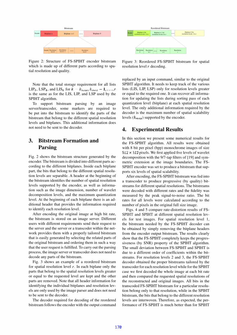
Figure 2: Structure of FS-SPIHT encoder bitstreamwhich is made up of different parts according to spa-tial resolution and quality.

Note that the total storage requirement for all listsLIP , LSP , and LIS for b K g!#"$"$"$j|is the same as for the LIS, LIP, and LSP used by theSPIHT algorithm.

To support bitstream parsing by an imageserver/transcoder, some markers are required tobe put into the bitstream to identify the parts of thebitstream that belong to the different spatial resolutionlevels and bitplanes. This additional information doesnot need to be sent to the decoder.

3. Bitstream Formation andParsing

Fig. 2 shows the bitstream structure generated by theencoder. The bitstream is divided into different parts ac-cording to the different bitplanes. Inside each bitplanepart, the bits that belong to the different spatial resolu-tion levels are separable. A header at the beginning ofthe bitstream identifies the number of spatial resolutionlevels supported by the encoder, as well as informa-tion such as the image dimension, number of waveletdecomposition levels, and the maximum quantizationlevel. At the beginning of each bitplane there is an ad-ditional header that provides the information requiredto identify each resolution level.

After encoding the original image at high bit rate,the bitstream is stored on an image server. Differentusers with different requirements send their request tothe server and the server or a transcoder within the net-work provides them with a properly tailored bitstreamthat is easily generated by selecting the related parts ofthe original bitstream and ordering them in such a waythat the user request is fulfilled. To carry out the parsingprocess, the image server or transcoder does not need todecode any parts of the bitstream.

Fig. 3 shows an example of a reordered bitstreamfor spatial resolution level | . In each biplane only theparts that belong to the spatial resolution levels greateror equal to the requested level are kept and the otherparts are removed. Note that all header information foridentifying the individual bitplanes and resolution lev-els are only used by the image parser and does not needto be sent to the decoder.

The decoder required for decoding of the reorderedbitstream follows the encoder with the output command

Figure 3: Reordered FS-SPIHT bitstream for spatialresolution level | decoding.

replaced by an input command, similar to the originalSPIHT algorithm. It needs to keep track of the variouslists (LIS, LIP, LSP) only for resolution levels greateror equal to the required one. It can recover all informa-tion for updating the lists during sorting pass of eachquantization level (bitplane) at each spatial resolutionlevel. The only additional information required by thedecoder is the maximum number of spatial scalabilitylevels ( ! ) supported by the encoder.

4. Experimental ResultsIn this section we present some numerical results forthe FS-SPIHT algorithm. All results were obtainedwith 8 bit per pixel (bpp) monochrome images of size ]~ ] pixels. We first applied five levels of waveletdecomposition with the 9/7-tap filters of [19] and sym-metric extension at the image boundaries. The FS-SPIHT encoder was set to produce a bitstream that sup-ports six levels of spatial scalability.

After encoding, the FS-SPIHT bitstream was fed intoa transcoder to produce progressive (by quality) bit-streams for different spatial resolutions. The bitstreamswere decoded with different rates and the fidelity wasmeasured by the peak signal-to-noise ratio. The bitrates for all levels were calculated according to thenumber of pixels in the original full size image.

Figs. 4 and 5 compare rate-distortion results of FS-SPIHT and SPIHT at different spatial resolution lev-els for test images. For spatial resolution level 1,the bitstream needed by the FS-SPIHT decoder canbe obtained by simply removing the bitplane headersfrom the encoder output bitstream. The results clearlyshow that the FS-SPIHT completely keeps the progres-siveness (by SNR) property of the SPIHT algorithm.The small deviation between FS-SPIHT and SPIHT isdue to a different order of coefficients within the bit-streams. For resolution levels 2 and 3, the FS-SPIHTdecoder obtained the proper bitstreams tailored by thetranscoder for each resolution level while for the SPIHTcase we first decoded the whole image at each bit rateand then compared the requested spatial resolutions ofthe reconstructed and original images. All bits in thetranscoded FS-SPIHT bitstream for a particular resolu-tion belong only to that resolution, while in the SPIHTbitstream, the bits that belong to the different resolutionlevels are interwoven. Therefore, as expected, the per-formance of FS-SPIHT is much better than for SPIHT

0 0.2 0.4 0.6 0.8 1 1.2 1.4 1.6 1.8 224

26

28

30

32

34

36

38

40

42

Rate (bpp)

PS

NR

(dB

)

SPIHTFS−SPIHT

0 0.1 0.2 0.3 0.4 0.5 0.6 0.7 0.8 0.9 120

25

30

35

40

45

50

Rate (bpp)

PS

NR

(dB

)

SPIHTFS−SPIHT

0 0.05 0.1 0.15 0.2 0.25 0.3 0.35 0.4 0.45 0.525

30

35

40

45

50

55

60

65

70

75

Rate (bpp)

PS

NR

(dB

)

SPIHTFS−SPIHT

Figure 4: Comparison of rate-distortion results for theGoldhill test image at different spatial resolution levels.Top: level 1 (original image size

&r ] ); middle:level 2 ( \ b \ ); bottom: level 3 ( &!&! ).for resolution levels greater than one. As the resolutionlevel increases, the difference between FS-SPIHT andSPIHT becomes more and more significant. All the re-sults are obtained without extra arithmetic coding ofthe output bits. As shown in [7], an improved codingperformance (about 0.3-0.6 dB) for SPIHT and conse-quently for FS-SPIHT can be achieved by further com-pressing the binary bitstreams with an arithmetic coder.

0 0.2 0.4 0.6 0.8 1 1.2 1.4 1.6 1.8 220

22

24

26

28

30

32

34

36

38

40

42

44

Rate (bpp)

PS

NR

(dB

)

SPIHTFS−SPIHT

0 0.1 0.2 0.3 0.4 0.5 0.6 0.7 0.8 0.9 120

25

30

35

40

45

50

Rate (bpp)

PS

NR

(dB

)

SPIHTFS−SPIHT

0 0.05 0.1 0.15 0.2 0.25 0.3 0.35 0.4 0.45 0.525

30

35

40

45

50

55

60

65

70

Rate (bpp)

PS

NR

(dB

)

SPIHTFS−SPIHT

Figure 5: Comparison of rate-distortion results for theBarbara test image at different spatial resolution levels.Top: level 1 (original image size

&r ] ); middle:level 2 ( \ \ ); bottom: level 3 ( &!&! ).5. Conclusions

We have presented a fully scalable SPIHT algorithmthat produces a bitstream which supports spatial scala-bility and can be used for multiresolution transcoding.This bitstream not only has spatial scalability featuresbut also keeps the full SNR embeddedness property forany required resolution level after a simple reordering

which can be done in a transcoder without decodingthe bitstream. The embeddedness is so fine granularthat almost each additional bit improves the quality, andthe bitstream can be stopped at any point to meet a bitbudget during the coding or decoding process. The pro-posed multiresolution image codec is a good candidatefor multimedia applications such as image storage andretrieval systems, progressive web browsing and mul-timedia information transmission, especially over het-erogenous networks where a wide variety of users needto be differently serviced according to their network ac-cess and data processing capabilities.

References

[1] D. S. Taubman and M. W. Marcellin, Jpeg2000:Image Compression Fundamentals, Standards,and Practice, Kluwer, Boston, MA, 2002.

[2] C. Christopoulos, A. Skordas, and T. Ebrahimi,“The jpeg2000 still image coding system: anoverview,” IEEE Trans. Consumer Electronics,vol. 46, no. 4, pp. 1103–1127, Nov. 2000.

[3] J. M. Shapiro, “Embedded image coding usingzerotree of wavelet coefficients,” IEEE Trans.Signal Processing, vol. 41, pp. 3445–3462, Dec.1993.

[4] A. Zandi, J. D. Allen, E. L. Schwartz, andM. Boliek, “CREW: Compression with revesibleembedded wavelet,” in Proc. IEEE Data Com-pression Conf., Mar. 1995, pp. 212–221.

[5] Y. Chen and W. A. Pearlman, “Three-dimentionalsubband coding of video using the zero-treemethod,” in Proc. SPIE 2727-VCIP’96, Mar.1996, pp. 1302–1309.

[6] S. A. Martucci and I. Sodagar, “Entropy codingof wavelet coefficientsfor very low bit rate video,”in Proc. IEEE Int. Conf. Image Processing, Sept1996, vol. 2, pp. 533–536.

[7] A. Said and W. A. Pearlman, “A new, fast andefficient image codec based on set partitioning inhierarchical trees,” IEEE Trans. Circ. and Syst.for Video Technology, vol. 6, pp. 243–250, June1996.

[8] J. Liang, “Highly scalable image coding for mul-timedia applicatioans,” in Proc. ACM Multimedia97, Nov. 1997, pp. 11–19.

[9] Q. Wang and M. Ghanbari, “Scalable coding ofvery high resolution video using the virtual ze-rotree,” IEEE Trans. Circ. and Syst. for VideoTechnology, vol. 7, no. 5, pp. 719–727, Oct. 1997.

[10] S. A. Martucci, I. Sodagar, T. Chiang, and Y.-Q.Zhang, “A zerotree wavelet video coder,” IEEETrans. Circ. and Syst. for Video Technology, vol.7, no. 1, pp. 109–118, Feb. 1997.

[11] B.-J.Kim and W. A. Pearlman, “An embeddedvideo coder using three-dimensional set partition-ing in hierarchical trees (SPIHT),” in proc. IEEE

Data Compression Conf., Mar. 1997, pp. 251–260.

[12] J. Karlenkar and U. B. Desai, “SPIHT videocoder,” in Proc. IEEE Region 10 InternationalConference on Glaobal Connectivity in Energy,Computer, Communication and Control, TEN-CON’98, 1998, vol. 1, pp. 45–48.

[13] B.-J. Kim, Z. Xiong, and W. A. Pearlman, “Lowbit-rate scalable video coding with 3-d set parti-tioning in hierarchical trees (3-D SPIHT),” IEEETrans. Circ. and Syst. for Video Technology, vol.10, no. 8, pp. 1374–1387, Dec. 2000.

[14] J. Zho and S. Lawson, “Improvements of theSPIHT for image coding by wavelet transform,”in Proc. IEE Seminar on Time-scale and Time-Frequency Analysis and Applications (Ref. No.2000/019), 2000, pp. 24/1 –24/5.

[15] E. Khan and M. Ghanbari, “Very low bit ratevideo coding using virtual spiht,” IEE Electron-ics Letters, vol. 37, no. 1, pp. 40–42, Jan. 2001.

[16] H. Cai and B. Zeng, “A new SPIHT algorithmbased on variable sorting thresholds,” in Proc.IEEE Int. Symp. Circuits and Systems, May 2001,vol. 5, pp. 231–234.

[17] J. Y. Tham, S. Ranganath, and A. A. Kassim,“Highly scalable wavelet-based video codec forvery low bit-rate environment,” IEEE J. Select.Areas Commun., vol. 16, no. 1, pp. 12–27, Jan.1998.

[18] H. Danyali and A. Mertins, “Highly scalable im-age compression based on SPIHT for network ap-plications,” in Proc. IEEE Int. Conf. Image Pro-cessing, Rochester, NY, USA, Sept. 2002, inpress.

[19] M. Antonini, M. Barlaud, P. Mathieu, andI. Daubechies, “Image coding using wavelettransform,” IEEE Trans. Image Processing, vol.1, pp. 205–220, Apr. 1992.

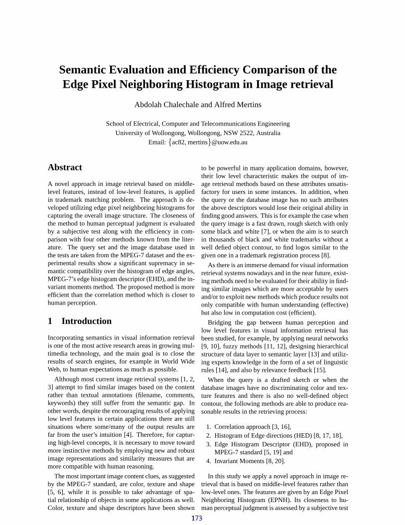
Semantic Evaluation and Efficiency Comparison of theEdge Pixel Neighboring Histogram in Image retrieval

Abdolah Chalechale and Alfred Mertins

School of Electrical, Computer and Telecommunications Engineering

University of Wollongong, Wollongong, NSW 2522, Australia

Email: ac82, mertins@uow.edu.au

Abstract

A novel approach in image retrieval based on middle-level features, instead of low-level features, is appliedin trademark matching problem. The approach is de-veloped utilizing edge pixel neighboring histograms forcapturing the overall image structure. The closeness ofthe method to human perceptual judgment is evaluatedby a subjective test along with the efficiency in com-parison with four other methods known from the liter-ature. The query set and the image database used inthe tests are taken from the MPEG-7 dataset and the ex-perimental results show a significant supremacy in se-mantic compatibility over the histogram of edge angles,MPEG-7’s edge histogram descriptor (EHD), and the in-variant moments method. The proposed method is moreefficient than the correlation method which is closer tohuman perception.

1 Introduction

Incorporating semantics in visual information retrievalis one of the most active research areas in growing mul-timedia technology, and the main goal is to close theresults of search engines, for example in World WideWeb, to human expectations as much as possible.

Although most current image retrieval systems [1, 2,3] attempt to find similar images based on the contentrather than textual annotations (filename, comments,keywords) they still suffer from the semantic gap. Inother words, despite the encouraging results of applyinglow level features in certain applications there are stillsituations where some/many of the output results arefar from the user’s intuition [4]. Therefore, for captur-ing high-level concepts, it is necessary to move towardmore instinctive methods by employing new and robustimage representations and similarity measures that aremore compatible with human reasoning.

The most important image content clues, as suggestedby the MPEG-7 standard, are color, texture and shape[5, 6], while it is possible to take advantage of spa-tial relationship of objects in some applications as well.Color, texture and shape descriptors have been shown

to be powerful in many application domains, however,their low level characteristic makes the output of im-age retrieval methods based on these attributes unsatis-factory for users in some instances. In addition, whenthe query or the database image has no such attributesthe above descriptors would lose their original ability infinding good answers. This is for example the case whenthe query image is a fast drawn, rough sketch with onlysome black and white [7], or when the aim is to searchin thousands of black and white trademarks without awell defied object contour, to find logos similar to thegiven one in a trademark registration process [8].

As there is an immerse demand for visual informationretrieval systems nowadays and in the near future, exist-ing methods need to be evaluated for their ability in find-ing similar images which are more acceptable by usersand/or to exploit new methods which produce results notonly compatible with human understanding (effective)but also low in computation cost (efficient).

Bridging the gap between human perception andlow level features in visual information retrieval hasbeen studied, for example, by applying neural networks[9, 10], fuzzy methods [11, 12], designing hierarchicalstructure of data layer to semantic layer [13] and utiliz-ing experts knowledge in the form of a set of linguisticrules [14], and also by relevance feedback [15].

When the query is a drafted sketch or when thedatabase images have no discriminating color and tex-ture features and there is also no well-defined objectcontour, the following methods are able to produce rea-sonable results in the retrieving process:

1. Correlation approach [3, 16],2. Histogram of Edge directions (HED) [8, 17, 18],3. Edge Histogram Descriptor (EHD), proposed in

MPEG-7 standard [5, 19] and4. Invariant Moments [8, 20].

In this study we apply a novel approach in image re-trieval that is based on middle-level features rather thanlow-level ones. The features are given by an Edge PixelNeighboring Histogram (EPNH). Its closeness to hu-man perceptual judgment is assessed by a subjective test

1

along with its efficiency in comparison with the abovefour methods. The evaluation, without losing generality,is made in solving the problem of trademark matching,where the query set and the image database are takenfrom the known and accessible MPEG-7 dataset.

The method utilizing EPNH for capturing the overallimage structure and its comprehensive details is given inthe next section. In Section 3 the description of the otherfour methods, used in our tests, is briefly provided. Sec-tion 4 shows the experimental results. An analysis anddiscussion of the results is given in Section 5. Section 6concludes the paper and suggests some further researchdirections in this area.

2 The Edge Pixel NeighboringHistogram (EPNH)

The main objective of the proposed method is to trans-form the image data into a new structure that supportsmeasurement of the similarity between images in a cor-rect, easy and fast way with emphasis on capturing moreconceptual meaning. Using histograms is recognized asa powerful tool in image retrieval. Several kinds of his-tograms and related similarity measuring techniques areproposed for comparing images based on color, textureand shape [5, 6]. Moreover, using an edge direction his-togram has been used as a discriminating cue especiallyin the absence of color information or in the presence ofimages with similar colors [17, 18].

EPNH is a novel approach that focuses on higher-level edge distribution rather than edge-based or pixel-distribution based methods. In this approach, the infor-mation about neighbors of edge pixels is obtained firstand then used to produce the neighboring histogram.

Initially, the images may have color attributes, andthey may be composed of single or multiple objects.Color images are converted to a gray intensity by elim-inating the hue and saturation while retaining the lumi-nance in a pre-processing stage. Gray scale, black &white and sketched images are not needed go throughthis process. Then, applying the Canny edge operator[21] on the image will result in an edge map,I, that isthe basic platform for obtaining the edge pixel neighbor-ing histogram. The histogram originally has 240 binsand the frequencies of edge pixels with similar neigh-boring code are stored in appropriate bins. The neigh-boring code is defined using the following edge pixel-neighboring diagram (see Fig. 1). In this diagram thecenter is an edge pixel inI. Considering 8-connectivity,each pixel has up to 4 neighbors in most cases, as thepixel and the neighbors are all edge points.

By numbering the directions as indicated in Fig. 1each pixel neighborhood is coded with a numbern with0 ≤ n ≤ 240; that is the sum of all direction numbersof its neighbors. For instance,n = 0 means a singularpoint (without any neighbor), a pixel point with two hor-izontal neighbors hasn = 17 (1+16) neighboring code

Figure 1: Edge Pixel-Neighboring Diagram.

andn = 240 means a point with 4 neighbors in the di-rections represented by 128, 64, 32 and 16. This codeindicates the structure of the neighbor pixels for eachpixel in the edge map. Figure 2 shows an example. Anedge pixel with one edge neighbor in the northern direc-tion (4), one neighbor in the western direction (16) andanother neighbor in the southeastern direction (128) hasthe unique number 148 (4+16+128) for its neighboringcode. The existence and the frequency of this structurein an edge map is an important feature and can be usedfor measuring the similarity between the correspondingimages.

Figure 2: An edge point with three neighbors.

The frequencies of the neighborhood codes(n 6= 0)form the EPNH bins. The singular points(n = 0) arescarce and not considered, and the sum of other edgepixels with the same neighboring code is stored in theappropriate bins.

The proposed numbering scheme simplifies the codefinding process since we only set a bit in the appropriateposition in the code byte indicated by the direction ofthe neighbor. Also, we can easily recognize the num-ber of neighbors by counting the number of ones in thecorresponding codes. The emphasis in this histogramis on the number of occurrences (frequencies) of eachcode and not on the code itself. Therefore, the overallstructure of the edge map image is captured in a his-togram representation which can be used for measuringthe similarity between images by any histogram inter-section techniques or simply by`1 or `2 distances.

The histogram entries depend on the size of the im-age and a normalization is required. Normalization ofEPNH is made by considering the size of the imagerather than the number of edge points. Brandt et al. usedthis type of normalization in their work and they arguedthat it is better than normalizing by the number of edge

2

points [22]. The normalized histogram is produced asfollows:

EPNHi =∑

i Pi

sizeI

1 ≤ i ≤ 240 andPi is any edge pixel inI with n = i.

The EPNH is translation and scale invariant, and be-cause of its middle-level feature, it captures more se-mantics in the image than the low-level methods. Be-cause the edge neighborhood feature is local, it is ro-bust to partial occlusion and local disturbance in the im-age. The rotation invariance property is achievable inthis method by grouping rotation-similar bins of the his-togram.

The histogram was recently used together with avicinity table and a specific similarity measure in sketchbased image retrieval [7]. It demonstrated a significantimprovement in retrieving images in a prototype imagedataset. In Section 4, it is shown that the EPNH can alsoproduce results that are much closer to human percep-tion than the results obtained from the edge directionhistogram, invariant moments and the MPEG-7’s edgehistogram descriptor.

3 Alternative Methods

In this section, the description of three edge-based meth-ods and the invariant moments method are addressed.In Section 4, they will be compared with the EPNHmethod.

3.1 Correlation Approach

The Query by Visual Example (QVE) system developedby Hirata and Kato [16] performs retrieval by computingthe correlation between the query sketch and databaseedge images. In this approach, the query and targetimages are resized to64 × 64 pixels and then the pro-posed gradient operator extracts their edges. The result-ing edge maps are called pictorial indexes and used forimage-to-image matching. After dividing each pictorialindex image into 64 blocks of equal size, the correla-tion between corresponding blocks in the query indexqand the database indexp is calculated by the followingbit-wise summation with shifting blocks ofq by δ andεover blocks ofp:

Cδε =∑s

∑r

(αprs · qr+δs+ε + βprs · qr+δs+ε

+ γprs ⊕ qr+δs+ε)(1)

The coefficientsα, β andγ are control parameters usedto estimate matching and mismatching patterns and takeup values 10, 1 and -3, respectively. The maximumvalue ofCδε for all δ andε for each block is called thelocal correlation factorC:

C = max(Cδε) for − 4 ≤ δ ≤ 4 and − 4 ≤ ε ≤ 4.

Finally, a global correlation factorCt that is the sumof all 64 C ’s, is calculated and used as the similaritymeasurement. A modified version of this method is usedin QBIC system by IBM [3].

Although the method has a good ability to find similarimages in small datasets [16] it does not allow indexing,and because of the expensive computational cost, usingthat method in a large image databases is time consum-ing. While the method can tolerate a small local rota-tion, it is not rotation invariant and does not allow forlarge global rotation.

3.2 Histogram of Edge Directions

Histogram of edge directions (HED) for representingimage information is one of the well-known methods inthe image retrieval literature. M. Abdel-Mottaleb [18]used this method by applying the Canny edge opera-tor to find strong edges in an image and then quantizedthem into only 4 directions (horizontal, vertical, and thetwo diagonals) to build histograms of edge directionsfor different image regions. The histograms are thenused as hash values in a hash table indexing mechanism.Jain and Vailaya [17] used edge directions as an imageattribute for shape description. They show that in theabsence of color information or in images with similarcolors this histogram is a significant tool in searchingfor similar images. They also exploited the histogramtogether with invariant moments in a case study usinga trademark image database [8]. The edge informationcontained in the database images is extracted off-line us-ing the Canny edge operator and then the correspondingedge directions are quantized into 72 bins of5 each. Toreduce the effect of rotation, they smooth the histogramas follows:

Is[i] =

∑i+kj=i−k I[j]2k + 1

whereIs is the smoothed histogram,I is the originalnormalized histogram, and the parameterk determinesthe degree of smoothing. In their experiments they usedk = 1.

3.3 MPEG-7 Edge Histogram Descriptor(EHD)

The MPEG-7 standard defines the edge histogram de-scriptor (EHD) in its texture part [5]. The distribution ofedges is not only a good texture signature it is also usefulfor image-to-image matching in the absence of any ho-mogeneous texture. A given image is first divided into16 sub-images (4 × 4), and local edge histograms arecomputed for each sub-image. Edges are grouped intofive classes: vertical, horizontal,45 diagonal,135 di-agonal, and isotropic (non-directional). The directionaledge strengths are obtained for each edge class using 5corresponding2 × 2 filter masks. If the maximum isgrater than a threshold value(Thedge) then the underly-ing block is designated to belong to the corresponding

3

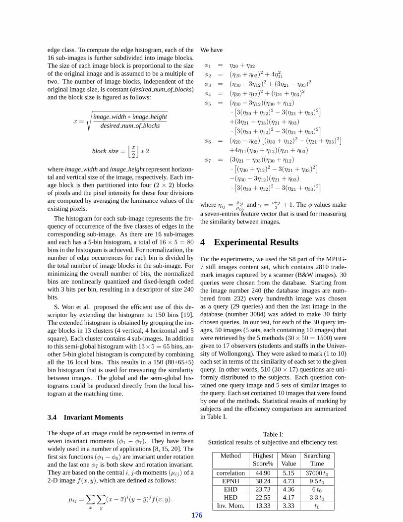
edge class. To compute the edge histogram, each of the16 sub-images is further subdivided into image blocks.The size of each image block is proportional to the sizeof the original image and is assumed to be a multiple oftwo. The number of image blocks, independent of theoriginal image size, is constant (desirednumof blocks)and the block size is figured as follows:

x =

√imagewidth∗ imageheight

desirednumof blocks

block size=⌊x

2

⌋∗ 2

whereimagewidthandimageheightrepresent horizon-tal and vertical size of the image, respectively. Each im-age block is then partitioned into four (2 × 2) blocksof pixels and the pixel intensity for these four divisionsare computed by averaging the luminance values of theexisting pixels.

The histogram for each sub-image represents the fre-quency of occurrence of the five classes of edges in thecorresponding sub-image. As there are 16 sub-imagesand each has a 5-bin histogram, a total of16 × 5 = 80bins in the histogram is achieved. For normalization, thenumber of edge occurrences for each bin is divided bythe total number of image blocks in the sub-image. Forminimizing the overall number of bits, the normalizedbins are nonlinearly quantized and fixed-length codedwith 3 bits per bin, resulting in a descriptor of size 240bits.

S. Won et al. proposed the efficient use of this de-scriptor by extending the histogram to 150 bins [19].The extended histogram is obtained by grouping the im-age blocks in 13 clusters (4 vertical, 4 horizontal and 5square). Each cluster contains 4 sub-images. In additionto this semi-global histogram with13×5 = 65 bins, an-other 5-bin global histogram is computed by combiningall the 16 local bins. This results in a 150 (80+65+5)bin histogram that is used for measuring the similaritybetween images. The global and the semi-global his-tograms could be produced directly from the local his-togram at the matching time.

3.4 Invariant Moments

The shape of an image could be represented in terms ofseven invariant moments(φ1 − φ7). They have beenwidely used in a number of applications [8, 15, 20]. Thefirst six functions(φ1 − φ6) are invariant under rotationand the last oneφ7 is both skew and rotation invariant.They are based on the centrali, j-th moments(µij) of a2-D imagef(x, y), which are defined as follows:

µij =∑

x

∑y

(x− x)i(y − y)jf(x, y).

We have

φ1 = η20 + η02

φ2 = (η20 + η02)2 + 4η211

φ3 = (η30 − 3η12)2 + (3η21 − η03)2

φ4 = (η30 + η12)2 + (η21 + η03)2

φ5 = (η30 − 3η12)(η30 + η12)· [3(η30 + η12)2 − 3(η21 + η03)2

]

+(3η21 − η03)(η21 + η03)· [3(η30 + η12)2 − 3(η21 + η03)2

]

φ6 = (η20 − η02)[(η30 + η12)2 − (η21 + η03)2

]

+4η11(η30 + η12)(η21 + η03)φ7 = (3η21 − η03)(η30 + η12)

· [(η30 + η12)2 − 3(η21 + η03)2]

−(η30 − 3η12)(η21 + η03)· [3(η30 + η12)2 − 3(η21 + η03)2

]

whereηij = µij

µγ00

andγ = i+j2 + 1. Theφ values make

a seven-entries feature vector that is used for measuringthe similarity between images.

4 Experimental Results

For the experiments, we used the S8 part of the MPEG-7 still images content set, which contains 2810 trade-mark images captured by a scanner (B&W images). 30queries were chosen from the database. Starting fromthe image number 240 (the database images are num-bered from 232) every hundredth image was chosenas a query (29 queries) and then the last image in thedatabase (number 3084) was added to make 30 fairlychosen queries. In our test, for each of the 30 query im-ages, 50 images (5 sets, each containing 10 images) thatwere retrieved by the 5 methods (30× 50 = 1500) weregiven to 17 observers (students and staffs in the Univer-sity of Wollongong). They were asked to mark (1 to 10)each set in terms of the similarity of each set to the givenquery. In other words, 510 (30× 17) questions are uni-formly distributed to the subjects. Each question con-tained one query image and 5 sets of similar images tothe query. Each set contained 10 images that were foundby one of the methods. Statistical results of marking bysubjects and the efficiency comparison are summarizedin Table I.

Table I:Statistical results of subjective and efficiency test.

Method Highest Mean SearchingScore% Value Time

correlation 44.90 5.15 37000 t0EPNH 38.24 4.73 9.5 t0EHD 23.73 4.36 6 t0HED 22.55 4.17 3.3 t0

Inv. Mom. 13.33 3.33 t0

4

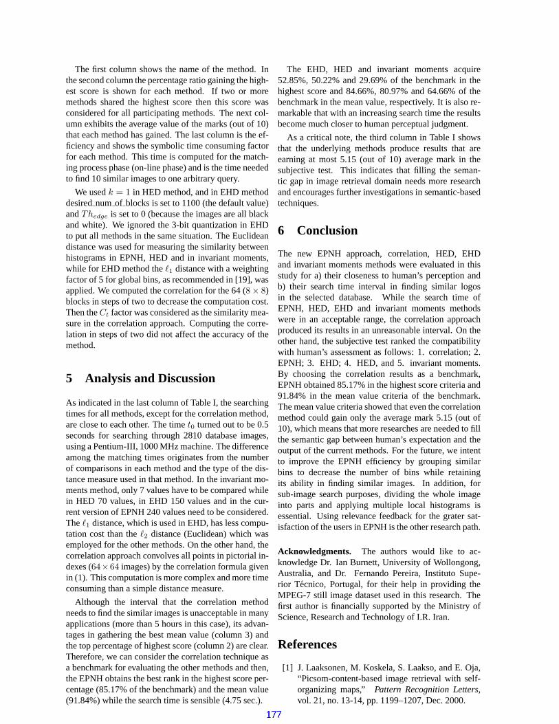
The first column shows the name of the method. Inthe second column the percentage ratio gaining the high-est score is shown for each method. If two or moremethods shared the highest score then this score wasconsidered for all participating methods. The next col-umn exhibits the average value of the marks (out of 10)that each method has gained. The last column is the ef-ficiency and shows the symbolic time consuming factorfor each method. This time is computed for the match-ing process phase (on-line phase) and is the time neededto find 10 similar images to one arbitrary query.

We usedk = 1 in HED method, and in EHD methoddesirednum of blocks is set to 1100 (the default value)andThedge is set to 0 (because the images are all blackand white). We ignored the 3-bit quantization in EHDto put all methods in the same situation. The Euclideandistance was used for measuring the similarity betweenhistograms in EPNH, HED and in invariant moments,while for EHD method the1 distance with a weightingfactor of 5 for global bins, as recommended in [19], wasapplied. We computed the correlation for the 64 (8× 8)blocks in steps of two to decrease the computation cost.Then theCt factor was considered as the similarity mea-sure in the correlation approach. Computing the corre-lation in steps of two did not affect the accuracy of themethod.

5 Analysis and Discussion

As indicated in the last column of Table I, the searchingtimes for all methods, except for the correlation method,are close to each other. The timet0 turned out to be 0.5seconds for searching through 2810 database images,using a Pentium-III, 1000 MHz machine. The differenceamong the matching times originates from the numberof comparisons in each method and the type of the dis-tance measure used in that method. In the invariant mo-ments method, only 7 values have to be compared whilein HED 70 values, in EHD 150 values and in the cur-rent version of EPNH 240 values need to be considered.The`1 distance, which is used in EHD, has less compu-tation cost than the2 distance (Euclidean) which wasemployed for the other methods. On the other hand, thecorrelation approach convolves all points in pictorial in-dexes (64×64 images) by the correlation formula givenin (1). This computation is more complex and more timeconsuming than a simple distance measure.

Although the interval that the correlation methodneeds to find the similar images is unacceptable in manyapplications (more than 5 hours in this case), its advan-tages in gathering the best mean value (column 3) andthe top percentage of highest score (column 2) are clear.Therefore, we can consider the correlation technique asa benchmark for evaluating the other methods and then,the EPNH obtains the best rank in the highest score per-centage (85.17% of the benchmark) and the mean value(91.84%) while the search time is sensible (4.75 sec.).

The EHD, HED and invariant moments acquire52.85%, 50.22% and 29.69% of the benchmark in thehighest score and 84.66%, 80.97% and 64.66% of thebenchmark in the mean value, respectively. It is also re-markable that with an increasing search time the resultsbecome much closer to human perceptual judgment.

As a critical note, the third column in Table I showsthat the underlying methods produce results that areearning at most 5.15 (out of 10) average mark in thesubjective test. This indicates that filling the seman-tic gap in image retrieval domain needs more researchand encourages further investigations in semantic-basedtechniques.

6 Conclusion

The new EPNH approach, correlation, HED, EHDand invariant moments methods were evaluated in thisstudy for a) their closeness to human’s perception andb) their search time interval in finding similar logosin the selected database. While the search time ofEPNH, HED, EHD and invariant moments methodswere in an acceptable range, the correlation approachproduced its results in an unreasonable interval. On theother hand, the subjective test ranked the compatibilitywith human’s assessment as follows: 1. correlation; 2.EPNH; 3. EHD; 4. HED, and 5. invariant moments.By choosing the correlation results as a benchmark,EPNH obtained 85.17% in the highest score criteria and91.84% in the mean value criteria of the benchmark.The mean value criteria showed that even the correlationmethod could gain only the average mark 5.15 (out of10), which means that more researches are needed to fillthe semantic gap between human’s expectation and theoutput of the current methods. For the future, we intentto improve the EPNH efficiency by grouping similarbins to decrease the number of bins while retainingits ability in finding similar images. In addition, forsub-image search purposes, dividing the whole imageinto parts and applying multiple local histograms isessential. Using relevance feedback for the grater sat-isfaction of the users in EPNH is the other research path.

Acknowledgments. The authors would like to ac-knowledge Dr. Ian Burnett, University of Wollongong,Australia, and Dr. Fernando Pereira, Instituto Supe-rior Tecnico, Portugal, for their help in providing theMPEG-7 still image dataset used in this research. Thefirst author is financially supported by the Ministry ofScience, Research and Technology of I.R. Iran.

References

[1] J. Laaksonen, M. Koskela, S. Laakso, and E. Oja,“Picsom-content-based image retrieval with self-organizing maps,” Pattern Recognition Letters,vol. 21, no. 13-14, pp. 1199–1207, Dec. 2000.

5

[2] M. Beigi, A. B Benitez, and S. Chang, “Metaseek:a content-based meta-search engine for images,”in Proceedings of Spie, USA, 1997, vol. 3312, pp.118–128.

[3] W. Niblack, R. Barber, W. Equitz, M. Flickner,E. Glasman, D. Petkovic, P. Yanker, C. Faloutsos,and G. Taubin, “The QBIC project: querying im-ages by content using color, texture, and shape,”in Proceedings of Spie, USA, 1993, vol. 1908, pp.173–187.

[4] H. W. Yoo, D. S. Jang, S. H. Jung, J. H. Park, andK. S. Song, “Visual information retrieval systemvia content-based approach,”Pattern Recognition,vol. 35, pp. 749–769, 2002.

[5] B. S. Manjunath, J.-R. Ohm, and V. V. Vasudevan,“Color and texture descriptors,”IEEE Transac-tions on Circuits and Systems for Video Technol-ogy, vol. 11, no. 6, pp. 703–715, June 2001.

[6] M. Bober, “Mpeg-7 visual shape descriptors,”IEEE Transactions on Circuits and Systems forVideo Technology, vol. 11, no. 6, pp. 716–719,June 2001.

[7] A. Chalechale and A. Mertins, “An abstract im-age representation based on edge pixel neighbor-hood information (EPNI),” infirst EurAsian con-ference on advances in information and communi-cation technology, 2002, In press.

[8] A. J. Jain and A. Vailaya, “Shape-based retrieval: acase study with trademark image databases,”Pat-tern Recognition, vol. 31, pp. 1369–1390, 1998.

[9] H. K. Lee and S. I. Yoo, “A neural network-based image retrieval using nonlinear combinationof heterogeneous features,” inIEEE proceedingsof the 2000 Congress on Evolutionary Computa-tion., 2000, vol. 1, pp. 667–674.

[10] Y. Kageyama and H. Saito, “Image retrieval sys-tem capable of learning the user’s sensibility usingneural networks,” inIEEE International Confer-ence on Neural Networks, 1997, vol. 3, pp. 1563–1567.

[11] Z. Wang, Z. Chi, and D. Feng, “Fuzzy integralfor leaf image retrieval,” inIEEE InternationalConference on Fuzzy Systems, Hong Kong, 2002,pp. 372–377.

[12] C. Vertan and N. Boujemaa, “Embedding fuzzylogic in content based image retrieval,” inIEEE19th International Conference of the North Amer-ican Fuzzy Information Processing Society, 2000,pp. 85–89.

[13] T. S. Chua, W.C Low, and T.M. Sim, “visual in-formation retrieval,” The Journal of the Institiute

of Image and Electronic Engineers of Japan, vol.27, pp. 10–19, 1998.

[14] C. Colombo, A. D. Bimbo, and P. Pala, “Semanticsin visual information retrieval,”IEEE Multimedia,vol. 6, no. 3, pp. 38–53, 1999.

[15] S. J. Yoon, D. K. Park, S. Park, and C. S. Won,“Image retrieval using a novel relevance feedbackfor edge histogram descriptor of Mpeg-7,” inpro-ceedings IEEE International Conference on Con-sumer Electronics, Piscataway, NJ, USA, 2001,pp. 354–355.

[16] K. Hirata and T. Kato, “Query by visual example-content based image retrieval,” inAdvances inDatabase Technology - EDBT ’92, Berlin, Ger-many, 1992, pp. 56–71.

[17] A. K. Jain and A. Vailaya, “Image retrieval usingcolor and shape,”Pattern Recognition, vol. 29, no.8, pp. 1233–1244, Aug. 1996.

[18] M. Abdel-Mottaleb, “Image retrieval based onedge representation,” inProceedings 2000 Inter-national Conference on Image Processing, Piscat-way, NJ, USA, 2000, vol. 3, pp. 734–737.

[19] C. S. Won, D. K. Park, and S Park, “Efficient useof Mpeg-7 edge histogram descriptor,”Etri Jour-nal, vol. 24, no. 1, pp. 23–30, Feb. 2002.

[20] D. Mohamad, G. Sulong, and S. S. Ipson, “Trade-mark matching using invariant moments,” inPro-ceedings second Asian Conference on ComputerVision, [ACVV’95]., Singapore, 1995, vol. 1, pp.439–444.

[21] J. Canny, “A computational approach to edge de-tection,” IEEE Transactions on Pattern Analysisand Machine Intelligence, vol. PAMI-8, no. 6, pp.679–698, Nov. 1986.

[22] S. Brandt, J. Laaksonen, and E. Oja, “Statisticalshape features in content-based image retrieval,”in Proceedings 15th International Conference onPattern Recognition. ICPR-2000, Los Almaitos,CA, USA, 2000, vol. 2, pp. 1062–1065.

6

STRUCTURED CODING FOR DISTRIBUTED HYPERAUDIO APPLICATIONS

Kathy Melih and Ruben Gonzalez K.Melih@gu.edu.au and R.Gonzalez@gu.edu.au

School of Information Technology, Griffith University, Gold Coast

PMB 50 Gold Coast Mail Centre, QLD 9726, Australia

Abstract Despite its promise, the WWW still falls far short of being a genuine hypermedia system. This situation is largely due to the continued dependence on non-structured representations of multimedia data. The audio domain in particular has received little attention in this area, perhaps because of the inherent difficulties posed by the medium. The authors have attempted to address this oversight by developing a structured audio representation designed specifically for audio retrieval. However, in today’s networked world, efficient transmission capabilities are also a priority. This paper addresses the issue of transmission efficiency by illustrating how the structure of the representation can be exploited for compression gain.

1. Introduction For all its ubiquity and promise to fulfil the now nearly 60 year old vision of Bush [1], the WWW continues to fall well short of delivering a genuine hypermedia experience. It is, instead, a sort of “multimedia enhanced” hypertext system. This situation is largely due to the continued dependence on non-structured representations of multimedia data, in general, and especially of audio data.

The reliance upon non-structured audio representations has arisen primarily from a desire to provide efficient storage and transmission mechanisms. However, this efficiency of storage and speedy delivery comes at a cost: ready access to vast volumes of information that are disorganised and difficult to access in a random fashion. Indeed, modern access mechanisms for audio have not progressed beyond the simple functions offered by even the earliest electronic audio recording and presentation devices: play, stop, pause, rewind, etc. Additionally, modern audio information management techniques are still either impractically complex to implement or too low level to be of general use.

In contrast to unstructured audio representations, the audio scene, as represented in the mind, is highly structured, with often complex mixtures, separated into individual acoustic ‘events’ or ‘objects’[7]. Further, when recalling a long audio ‘scenario’ (such as a speech or a piece of music) it is most natural to be able to recall individual events (such as a change of speaker or lead instrument) than precise, temporal locations relative to the beginning of the recording. However, the latter is essentially the only method available with unstructured audio representations.

Existing content-based access schemes do not provide a satisfactory solution to this situation as they are, in themselves, unstructured. Two general classes of content-based audio access exist: statistical and transcription mechanisms. Statistical methods provide very little information of relevance to the general user (a musician is not likely to be able to specify the centroid of the FFT of a cello tone, for example). Transcription methods, such as automatic speech/speaker recognition or MIDI/score based melody retrieval, can be useful in highly constrained environments. However, such methods cannot readily be used to generate the natural organisational structure that would be perceived in the audio signal. A transcription scheme is akin to a book containing only an index but no chapters, headings nor paragraphs. While the index can be useful, without any obvious organisation in the data, it is very difficult to gain a conceptual view of the information presented.

Clearly, there exists a duality between the need to provide efficient storage and transmission of audio data and the need for meaningful content-based access and retrieval mechanisms. With the present situation, attempts to resolve one of these problems simply exacerbates the other. The only feasible way of addressing both issues simultaneously is to provide a structured audio representation that provides useful information about the underlying data and allows the information to be structured to reflect either its original organisation or some user imposed organisation while at the same time providing for data compression.

The urgency of this requirement is most obvious in the light of the emerging MPEG-7 standard: “MPEG-7 shall support descriptors that can act as handles referring directly to the data, to allow manipulation of the multimedia material.” [2] That is, direct access to content information must be available in or along side the encoded data stream itself. Obviously, providing such access necessarily imposes a structure on the data.

The authors have previously described the low level aspects of a perceptually based, structured representation that was designed specifically to support the structured content-based access mechanisms mentioned above [3]. They further reported on the initial compression possibilities based on the lower levels of this representation [4]. They then went on to describe how a higher level of the structure can be derived from the representation [5] and outlined a framework for a hyperaudio model based on this structured representation [6]. It is thus timely that the issue of compression be

revisited in light of the higher level organisation that has been applied to the data.

2. Structured Audio 2 . 1 R e q u i r e d c h a r a c t e r i s t i c s .

A structured representation suitable for content-based retrieval must possess several key attributes. Firstly, the data must be divided into semantically relevant units. Secondly, these units should be individually decodable and randomly accessible. Further, it is desirable that these units be extracted automatically from a raw audio stream. Indeed, in the case of separating two simultaneously occurring units (speech over background music, for example) it is impossible to do so manually. Finally, useful information about the content of the unit should be co-located with the unit itself, since, as stated in the introduction, the current solution of including manually, or semi-automatically, generated transcriptions is far from ideal.

2 . 2 T h e A u d i o S t r u c t u r e

Figure 1 shows the structural decomposition of an audio stream facilitated by the developed representation.

AudioStreamAudio

Stream

AudioObjectAudioObject

AudioObjectAudioObject

AudioObjectAudioObject

TrackTrack TrackTrack NoiseburstNoiseburst

NoiseburstNoiseburst

TrackTrack TrackTrack

Harmonicgroup

Harmonicgroup

NoiseframeNoiseframe

Harmonicgroup

Harmonicgroup

Figure 1: Structuring audio using a perceptually based representation

The lowest level contains the perceptually relevant atomic features of an audio signal. These model the features extracted by the human auditory system at the lowest levels of auditory perception. Essentially two main classes of feature are extracted: a track and a noise burst. Tracks are further classified as either ‘tone’, ‘sweep’ or ‘formant’. Track formation is detailed in [3].

Harmonic groups and noise frames appear at the next highest level. The harmonic groups consist of tracks, co-located in time, that bear some resemblance to one another. In general, the frequencies of the tracks belonging to a single group will be harmonically related. Also, their frequency and amplitude contours will be scaled versions of a single ‘prototype’ contour. This property can be exploited to achieve compression gains for harmonic groups. This paper concerns itself with the compact representation of these groups. Noise frames consist of temporally adjacent noise bursts with similar characteristics (bandwidth, RMS power, spectral envelope, etc). The formation of mid-level groups was detailed in [5].

In order to provide for content-based random access, every element of the structure is randomly accessible and individually decodable. However, from a user’s

perspective, the lowest levels of the hierarchy are unlikely to have any relevance: a pure tone or sweep carries very little perceptually useful information. Hence, it is much more likely that a combination of at least two mid-level elements is required to create an inversion that is both intelligible and of acceptable quality. It follows that inverting an individual audio object should result in a signal that is both intelligible and of reasonable perceptual quality. It should also be apparent that, from both encoding and retrieval aspects, coding harmonic groups as individual objects is preferable to encoding individual tracks.

2 . 3 G e n e r a t i on a n d I n v e r s i o n

The structure described in the previous section is based on a representation that is modelled after that found in the early stages of human auditory perception. This representation consists of a series of time-frequency-amplitude trajectories that are non-uniformly sampled in each dimension. The trajectories are composed of amplitude peaks in the short-time spectra. These peaks are ‘tracked’ through time according to low-level psychoacoustic principles. An illustration of the basic elements is given in Figure 2.

Noise burst

Tone

Frequency

Time

Frequency sweep

Formant

Figure 2: Basic perceptual elements of auditory data

The basic process used to obtain the representation was detailed in [3] and is summarised in Figure 3. Incoming audio data is analysed to produce a TFD. The peaks in amplitude of this distribution are found and tracked through time and frequency. Each resultant track is then classified according to type (tone, noise or sweep). Finally, the tracks are grouped according to psychoacoustic principles and encoded in these groups.

Resynthesis

DHT analysis

Peak tracking

Peak picking

Acoustic masking

Σ Residual spectrum

Input signal

Frequency tracks

Track grouping

Structured representation

+ -

Figure 3 Coding algorithm

Having generated the representation, it may be inverted using the procedure illustrated in Figure 4. This inversion technique makes it possible to invert individual tracks or groups of tracks. This is consistent with the aim of maintaining access to individually decodeable, randomly accessible and semantically significant segments of audio.

Sinusoidal generator

Sinusoidal generator

Sinusoidal generator

ΣTrack

parameters

(frequency, phase, amplitude)

Output signal

Figure 4: Track inversion

3. Encoding the groups Having generated the tracks and formed them into harmonic groups it is then necessary to encode the groups to provide for efficient storage and retrieval. It is important to note however, that the structure revealed in both the individual tracks and the harmonic groups cannot be obfuscated. This is in contrast with traditional coding schemes that exploit statistical redundancies in the data at the expense of access to content or structural information. Hence the selection of coding techniques is somewhat limited and decisions must be made carefully.

3 . 1 F i l e s t r u c t u r e

In order for the basic aims of the representation to be achieved, it is imperative that the coded data be written to the file in a manner that explicitly maintains the structure of the underlying data. In addition, random access must be supported. These considerations ensure that the desire for compression does not override the fundamental aim of creating a structured representation suitable for higher level access mechanisms such as hyperaudio.

The proposed file structure consists of a 24 byte file identification and version code followed by a header that is a list of 32 bit values denoting the position of each harmonic group in the file. This list is terminated by a null code. Each harmonic group is preceded by its own header information as described in section 3.3.3. Since each harmonic group is effectively self contained, it is a simple matter for some higher level process to assign a new organisation to the groups by creating a list of pointers to individual groups of tracks. Further, if access to a single track is desired, the groups themselves are encoded in a structured manner ensuring that it is relatively straightforward to define a link to even a single track.

3 . 2 H a r m o n i c G r o u p D e s c r i p t i o n

It was stated in section 2.2 that the tracks comprising a harmonic group are essentially frequency- and amplitude- scaled versions of an individual ‘prototype’ or ‘model’ track. Thus the essential information that must be recorded for each harmonic group is:

(a) Number of tracks (harmonics) (b) Model Track class: TONE, SWEEP, FORMANT (c) Model Frequency v’s time contour (d) Harmonic number and freq offset of each track (e) Model Amplitude v’s time contour (f) Amplitude v’s harmonic scale factor for each track (g) Model Phase v’s time contour (h) Phase v’s harmonic phase offset for each track (i) Start and stop time of group model

(j) Start and stop time of each track within the group (relative to those of the group model).

The necessity to record items a), c)-e), g) and i) should be immediately apparent. The model track class (item c) provides inbuilt indexing since the shape of the tracks within a harmonic group provide information that can be used to determine the most likely audio source represented by the group. For example, ‘formant’ shaped tracks indicate speech. Given the tracks in a group are harmonically related, the harmonic number of each track relative to the model track is obviously required. A frequency offset from the exact harmonic frequency must also be recorded as harmonics of many natural sounds fall slightly ‘off centre’.

3 . 3 C o d i n g T e c h n i q u e s

Coding techniques for the individual tracks were suggested by the authors in [4]. Given the harmonic grouping now achieved it is possible to exploit the redundancy within a group to considerable advantage for coding gain. This is because we only have to store detailed information about a single track for each group with a small amount of overhead to accommodate the individual tracks within the group. To gain access to the details for an individual track, simple scaling or offset of the corresponding parameters for the group model track is all that is required. Hence, we can now achieve a much greater coding gain while maintaining direct access to the individual elements of the representation.

3.3.1 Amplitude and Frequency Contours

The amplitude and frequency contours for the tracks vary slowly in time. Hence, DPCM is an ideal way to encode them. To further increase the coding gain, variable length codewords can be used. This has particular advantages for tones and constant rate sweeps, where a very large proportion of transitions have a constant value (zero for tones, non-zero for sweeps).

Thus the first step in encoding the amplitude and frequency contour of each group model is to determine the numerical gradient of each of its contours:

( ) ( ) ( )iii tftftdf −= +1 and ( ) ( ) ( )iii tAtAtdA −= +1

where f(ti) and A(ti) represent the values of the frequency and amplitude contours respectively of the model track at time ti. Variable length codeword allocation is then performed by Huffman encoding these gradient functions.

Thus for each model contour the following quantities must be recorded: an initial value, the Huffman codebook and the Huffman encoded values themselves. The bit allocation required to encode the amplitude and frequency contours is summarised in Table 1.

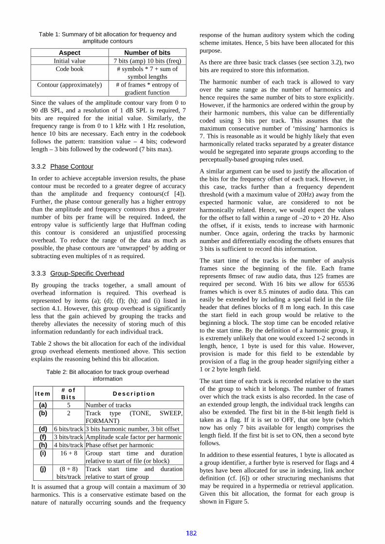
Table 1: Summary of bit allocation for frequency and amplitude contours

Aspect Number of bits Initial value 7 bits (amp) 10 bits (freq) Code book # symbols * 7 + sum of

symbol lengths Contour (approximately) # of frames * entropy of

gradient function Since the values of the amplitude contour vary from 0 to 90 dB SPL, and a resolution of 1 dB SPL is required, 7 bits are required for the initial value. Similarly, the frequency range is from 0 to 1 kHz with 1 Hz resolution, hence 10 bits are necessary. Each entry in the codebook follows the pattern: transition value – 4 bits; codeword length – 3 bits followed by the codeword (7 bits max).

3.3.2 Phase Contour

In order to achieve acceptable inversion results, the phase contour must be recorded to a greater degree of accuracy than the amplitude and frequency contours(cf [4]). Further, the phase contour generally has a higher entropy than the amplitude and frequency contours thus a greater number of bits per frame will be required. Indeed, the entropy value is sufficiently large that Huffman coding this contour is considered an unjustified processing overhead. To reduce the range of the data as much as possible, the phase contours are ‘unwrapped’ by adding or subtracting even multiples of π as required.

3.3.3 Group-Specific Overhead

By grouping the tracks together, a small amount of overhead information is required. This overhead is represented by items (a); (d); (f); (h); and (i) listed in section 4.1. However, this group overhead is significantly less that the gain achieved by grouping the tracks and thereby alleviates the necessity of storing much of this information redundantly for each individual track.

Table 2 shows the bit allocation for each of the individual group overhead elements mentioned above. This section explains the reasoning behind this bit allocation.

Table 2: Bit allocation for track group overhead information

I t e m # o f B i t s D e s c r i p t i o n

(a) 5 Number of tracks (b) 2 Track type (TONE, SWEEP,

FORMANT) (d) 6 bits/track 3 bits harmonic number, 3 bit offset (f) 3 bits/track Amplitude scale factor per harmonic (h) 4 bits/track Phase offset per harmonic (i) 16 + 8 Group start time and duration

relative to start of file (or block) (j) (8 + 8)

bits/track Track start time and duration relative to start of group

It is assumed that a group will contain a maximum of 30 harmonics. This is a conservative estimate based on the nature of naturally occurring sounds and the frequency

response of the human auditory system which the coding scheme imitates. Hence, 5 bits have been allocated for this purpose.

As there are three basic track classes (see section 3.2), two bits are required to store this information.

The harmonic number of each track is allowed to vary over the same range as the number of harmonics and hence requires the same number of bits to store explicitly. However, if the harmonics are ordered within the group by their harmonic numbers, this value can be differentially coded using 3 bits per track. This assumes that the maximum consecutive number of ‘missing’ harmonics is 7. This is reasonable as it would be highly likely that even harmonically related tracks separated by a greater distance would be segregated into separate groups according to the perceptually-based grouping rules used.

A similar argument can be used to justify the allocation of the bits for the frequency offset of each track. However, in this case, tracks further than a frequency dependent threshold (with a maximum value of 20Hz) away from the expected harmonic value, are considered to not be harmonically related. Hence, we would expect the values for the offset to fall within a range of –20 to + 20 Hz. Also the offset, if it exists, tends to increase with harmonic number. Once again, ordering the tracks by harmonic number and differentially encoding the offsets ensures that 3 bits is sufficient to record this information.

The start time of the tracks is the number of analysis frames since the beginning of the file. Each frame represents 8msec of raw audio data, thus 125 frames are required per second. With 16 bits we allow for 65536 frames which is over 8.5 minutes of audio data. This can easily be extended by including a special field in the file header that defines blocks of 8 m long each. In this case the start field in each group would be relative to the beginning a block. The stop time can be encoded relative to the start time. By the definition of a harmonic group, it is extremely unlikely that one would exceed 1-2 seconds in length, hence, 1 byte is used for this value. However, provision is made for this field to be extendable by provision of a flag in the group header signifying either a 1 or 2 byte length field.

The start time of each track is recorded relative to the start of the group to which it belongs. The number of frames over which the track exists is also recorded. In the case of an extended group length, the individual track lengths can also be extended. The first bit in the 8-bit length field is taken as a flag. If it is set to OFF, that one byte (which now has only 7 bits available for length) comprises the length field. If the first bit is set to ON, then a second byte follows.

In addition to these essential features, 1 byte is allocated as a group identifier, a further byte is reserved for flags and 4 bytes have been allocated for use in indexing, link anchor definition (cf. [6]) or other structuring mechanisms that may be required in a hypermedia or retrieval application. Given this bit allocation, the format for each group is shown in Figure 5.

•••

Group ID

8 bits

Rsvd flags 8 bits

User defined indexing/structure

32 bits

Type 2

bits Group start

time 16 bits

Group duration 8/16 bits

# (n) of tracks 5 bits

hn1 & fos1

6 bits hnn & fosn

6 bits

asf1 3

bits

asfn3

bits pos1

4 bits

posn 4

bits

•••

••• Group

duration 8/16 bits

Figure 5: Header format for each track group

4. Results To validate the technique, a simple yet representative test file is analysed. However, in terms of the grouping, even this simple data set poses a non trivial problem[5]. The file contains an artificially mixed combination of speech and music. The speech is a female speaker pronouncing the vowel ‘U’ while the music is the note b2 played on a piano. The two signals were artificially mixed such that the spoken utterance occurred simultaneously with the centre of the note. The input file is a windows PCM WAV file sampled at 32kHz with 16 bit resolution.

Figure 6 shows the results of the track formation and grouping algorithm illustrated in Figure 3. It may be surprising to note that the tonal tracks (corresponding to the solo piano tone) have been assigned to two separate harmonic groups. This is because the higher frequency harmonics of the piano tone do indeed correspond to a significantly different fundamental frequency. This can be seen in the illustration of the model tracks used to describe each of these groups found in Figure 7.

0 10 20 30 40 50 600

500

1000

1500

2000

2500

3000

3500

4000

4500

5000

freq

(Hz)

time (frames)

group 1group 2group 3

Figure 6: Tracks and groups generated for mixed source

data

To determine the amount of data required to encode each of these groups, the parameters mentioned in section 4 need to be derived. We must then perform a statistical analysis of each trajectory used to represent the model tracks and determine the remaining header information that pertains to each individual harmonic. The basic group duration and membership information is summarised in Table 3.

Table 3: Group duration and number of constituent tracks for each group in the mixed data set

G r o u p S t a r t f r a m e L e n g t h # o f

t r a c k s 1 0 59 16 2 0 49 8 3 7 37 18

The frequency contours of the model tracks are illustrated in Figure 7 and Figure 8 shows the frequency gradient functions of these. As is clearly evident, the data are highly correlated. Thus the motivation for using a statistically-based encoding scheme for these contours.

0 10 20 30 40 50 60140

160

180

200

220

240

260

280

freq

(Hz)

time (frames)

group 1group 2group 3

Figure 7: Frequency contours of models derived for track groups

0 10 20 30 40 50 60-8

-6

-4

-2

0

2

4

time (frames)

df (H

z)

group 1group 2group 3

Figure 8: Frequency gradient functions

Table 4 summarises the number of bits required to represent the frequency contours of each group. The codebook size and total number of bits required to code the gradient function were determined by generating the Huffman codes. The total figure appearing at the bottom of this table includes the 10 bits used to code the initial frequency value.

Table 4: Summary of bit allocation for the frequency contour of each group model

G r p 1 G r p 2 G r p 3 Number of symbols 6 4 11 Entropy 1.875 1.385 3.274 Codebook size in bits 62 38 120 Total bits for gradient function

92 82 113

Total bits for freq contour 164 130 243 Table 5 summarises the number of bits required to code the amplitude contours of the model tracks. The comments made for Table 4 similarly apply.

Legend Type ........ (b)# ...............(a)hn & fos .. (d)asf ............ (f)pos .......... (h)

Table 5: Summary of bit allocation for the amplitude contours of the group models

G r p 1 G r p 2 G r p 3 Number of symbols 6 6 8 Entropy 2.04 2.00 2.51 Codebook size in bits 62 64 85 Total bits for gradient function

121 95 92

Total bits for freq contour 190 166 184

0 10 20 30 40 50 60-4

-3.5

-3

-2.5

-2

-1.5

-1

-0.5

0

0.5

1

time (frames)

phas

e (ra

dian

s)

Figure 9: Phase 'contour' of each group model

Figure 9 shows the phase contours of the group models. It is clear that, unlike the frequency and amplitude data, the phase data are highly uncorrelated. Thus, performing Huffman coding would increase the coding complexity with little or no corresponding compression gain. Hence fixed length codewords are used. The codeword length is determined by the range of phase values for the track and the precision required, which is 3 significant figures. The first 4 bits of the phase description indicates this length.

Table 6: Summary of bit allocation for phase contours of group model

M i n V a l u e

M a x V a l u e

B i t s p e r

f r a m e

T o t a l b i t s f o r

t r a c k G r o u p 1 -1.95 0.85 9 535 G r o u p 2 -1.23 2.31 9 445 G r o u p 3 -0.49 0.57 7 263 Finally, Table 7 summarises the bit allocation for the mixed data file.

Table 7: Summary of bit allocation for all track elements in the mixed data file

I t e m G r o u p 1 G r o u p 2 G r o u p 3 (a) 5 5 5 (b) 2 2 2 (c) 164 130 243 (d) 96 48 108 (e) 190 166 184 (f) 48 24 54 (g) 535 445 263 (h) 64 32 72 (i) 24 24 24 (j) 16 16 16

head 50 50 50 Total 1194 944 1024

Table 7 shows that a total of 3215 bits is required to describe the track data. In addition to this the file contains a 24 byte general file header and an index header requiring of 32 bits/group plus an additional 32 bits to terminate the header. This gives a total file size of 3439 bits = 430 bytes. The original file size was 34,860 bytes hence a compression ratio of 81:1 has been achieved. However, this analysis has neglected one of the classes required in our structured data model: noise. It can be expected that the addition of the noise class will approximately half this value to give a compression ratio of approximately 40:1.

5. Discussion and conclusions The authors have presented a review of the development of a perceptually-based structured audio representation designed specifically to support audio information management and advanced applications such as hypermedia. This review was followed by an analysis of the representation’s suitability for compressed data storage by suggesting suitable coding techniques.

Having successfully extracted harmonic groups from the low-level track information, has facilitated the exploitation of redundancy in these harmonic groups. By doing so we have greatly improved upon the compression ratio of 9:1 achievable when each individual track is encoded separately. When reconstructed, subjective audio quality of each of the groups is sufficient to be recognised as the original source.

6. References [1] Bush, V., “As We May Think”, Atlantic Monthly, July

1945, 101-108. [2] ISO, “MPEG-7 Requirements Document V.9”, N2859,

Vancouver Canada, July 1999. [3] Melih, K. and Gonzalez, R., “Audio Retrieval Using

Perceptually Based Structures”, Proc. IEEE International Conf. On Multimedia Computing and Systems ’98, Austin, Texas, 28 June - 1 July 1998, 338-347.

[4] Melih, K. and Gonzalez, R., “Structured Coding for Content Based Interactive Audio”, Proc. IEEE International Conf. On Multimedia Computing and Systems ’99, Florence, Italy.

[5] Melih, K. and Gonzalez, R., “Source segmentation for Structured Audio”, Proceedings of the IEEE International Conference on Multimedia and Expo (ICME), New York, 2000.

[6] Melih, K. and Gonzalez, R., “Towards True Hyper-Audio”, ISPA 2001.

[7] Bregman, A.S., Auditory Scene Analysis: the Perceptual Organisation of Sound, MIT Press, 1990

185

AbstractThe view-based approach for representation ofhuman gestures and K -nearest neighbortechnique for classification is evaluated forper formance. The view based approach collapsestemporal component into gesture representationin a way that no explicit sequence matching ortemporal analysis is needed. This results in theconstruction of M otion History Image (M HI),which character izes the motion from a very highdimensional space to a low dimensional space.The seven Hu Image moments are computedfrom M HI, which are then modified to beinvar iant to translation, rotation and scale. Therecognition criter ion is established by a nearestneighbour techniqueusing M ahalanobisdistance.

Index Terms—Human gestures classification,motion based representation, spatio-temporal,M ahalanobis distance, computer vision, M otionHistory Image.

I . INTRODUCTION

Classification of human gestures is a verychallenging problem. The importance of humangesture classification is evident by the increasingrequirement of machines to be able to interactintelligently and effortlessly with a human inhabitedenvironment. However, to date, most of theinformation extracted by machines from humanmovement has been from static events such as a keypress. To improve machine capabilities in real timee.g. surveillance, human interaction with machinesand for helping disabled people, it is desirable torepresent motion from very high dimensional spaceto a low dimensional space without loss of truemotion characteristics.Past attempts reported in literature to recognizedynamic actions by machines require intrusivedevices that limit the scope of their applications tosituations where people specifically intend to

Arun Sharma, School of ECSE, RMIT University,Melbourne, Australia, e-mail: s9900960@student.rmit.edu.au

communicate with computers [1-9]. Other majorearly works involved the use of Moving LightDisplay (MLD) on subjects in a darkened room[10,11] and Structure from Motion (SFM) techniqueswhere a 3 dimensional model of the person isreconstructed to recognize the action [12-16]. WhileMLD was a useful experiment and demonstratedhuman perceptual abilities from motion informationalone, the MLD technique is very intrusive.Applications for the glove-based systems haveincluded remote computer-aided presentation [9] andfingertip tracking [8], but such systems lacknaturalness and robustness. Systems using SFM [9,17] techniques are more complex, computationallyexpensive, and also assume the hand to be a ‘ rigidobject’ , thereby greatly limiting theapplications.

This paper reports the research conducted toidentity simple pre-defined human gestures ofsubjects from video data using computationallysimple techniques that does not require the use ofintrusive devices and are not user dependent andlacking in naturalness. This is the first step towardsdeveloping applications where movement data maybe interpreted by machines in normal living andworking environments to identify the gestures or thesubject. Examples of such applications may includeidentification of messages, actions, status andidentity of individuals operating specific equipmentor inhabiting a specific environment. This will takethe capability of machines into the ‘understandingpeople’ domain.

This research has incorporated thetechniques proposed by Bobick and Davis [18, 19]Black and Yakoob [20] Romer Rosales & StanSclaroff [21] and is based on the use of view-basedrepresentation of gestures using Motion HistoryImage (MHI) (Figures 1-4). Our research has takenthe use of MHI and combined the same with imagemoment technique as proposed by Hu [22] to use itfor gross body movements. This paper reports theextension of the use of image moments [19, 23]with the use of statistical measures of similarity,Mahalanobis distance, applied to moment-basedfeatures extracted from MHI for the classification ofgestures.

Representation and Classification of HumanMovement Using Temporal Templates and Statistical

Measure of Similarity

Arun Sharma, Dinesh K Kumar, Sanjay Kumar, Neil McLachlan

186

I I .THEORY:AN OVERVIEW AND EXPLANATION OF THEAPPROACH

Based on research reported in literature, it can bestated that actions and messages can be recognizedby description of the appearance of motion [10, 11,19, 24-31] without reference to underlying staticimages, and without a full geometric reconstructionof the moving part [20]. It can also beargued that thestatic images produced using MHI based on theDifference of Frames (DOF) can represent featuresof temporally localized motion [32]. The advantageof this technique is the computational simplicity.Thispaper reports theefforts to verify this technique.

I I (a) REPRESENTATION OF M OTION:The DOF data from video recorded human

gestures are analysed by temporal integration of theframes covering the period of the distinct movement.The delimiters for the start and stop of the movementare added manually in the sequence. The temporalhistory of the movement in MHI is inserted into thedata by multiplication of the intensity of each framewith a linear ramp representing time. The MHI greyscale images are then generated by temporalintegration. This eliminates the need for timesequence coding. The process can be mathematicallyrepresented by thefollowing:

Let I(x, y, n) bean imagesequence& let

)1,,(),,(),,( −−= nyxInyxInyxD

where I(x, y, n) is the intensity of each pixel atlocation x, y at frame/time n and D(x, y, n), is thedifference of consecutive frames representingregions of motion. The difference is then thresholdedto a binary map that shows where there is highlikelihood of motion being present.

Γ>=

Otherwise0

),,(if1),,(

nyxDnyxB

whereΓ isselected threshold. Then theMHI isgiven

where N is total number of frames that capture themotion. The pixel intensity Hn is a function ofmotion history at that point and the result is a scalar-value image where more recently moving pixels arebrighter [19]. The Motion Energy Image (MEI),

which highlights the regions in the image where anyform of motion was present since the beginning ofthe action, can be generated by thresholding MHIabovezero.

I I (b) FEATURE EXTRACTION:

Figure. 1 Action: Lateral Arm Down Half-Way

The MHI images of human movementshave to be described in terms of suitable features forclassification. The grey levels are the temporaldescriptors and thus the analysis should be ‘globalinternal’ (region based) [33] instead of shapeboundary description and its features [34-36].

Given an arbitrary intensity function f(x,y),then the set of moments m pq (equation 1) have aproperty of fundamental importance: they uniquelydetermine, and are uniquely determined by, thefunction f(x,y). The moments m pq are sufficient toaccurately reconstruct the original function f(x,y)[37, 38]. For an appearance based, view sensitiveapproach, it is desirable to have matching techniquethat is as invariant as possible to the imagingsituation [18]. It needs to be invariant to translation(space in the image where object is represented),rotation and scaling. The moments defined byequation 1 are not ideal for MHI description sincethey are not invariant to translation, rotation andscale. To overcome this difficulty, modified sevenHu moments [22] (equation 3) areused

The calculation of the feature vectorsinvolves using normalized central moments(equation 2). These moments are reputed to beinvariant to affine transformations, such astranslation. Using these moments, the invariantnature of the feature vectors can be taken a stepfurther by applying a set of moment functions called,"Hu functions" which result in translation, rotationand scale invariant features. These invariants arebased on momentsup to third order.

The advantage of moment methods is thatthey are mathematically concise and for the intensityimage of MHI, reflect not only the shape but also thedensity distribution within it. Thus, the descriptors ofthe Motion templates of human gestures generated

×=−

=

nnyxByxH

N

n

n U1

1

),,(max),(

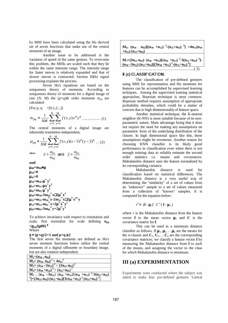
187

by MHI have been calculated using the Hu derivedset of seven functions that make use of the centralmomentsof an image.

Another issue to be addressed is thevariation of speed of the same gesture. To overcomethis problem, the MHIs are scaled such that they liewithin the same intensity range. The intensity rangefor faster moves is relatively expanded and that ofslower moves is contracted. Section III(b) signalprocessing-explains theprocess.

Seven Hu's equations are based on theuniqueness theory of moments. According touniqueness theory of moments for a digital image ofsize (N, M) the (p+q)th order moments mpq arecalculated

(For p, q =[0,1,2...])

= =

≡N

x

M

y

qppq yxyxf

NMm

1 1

),(1

……………. (1)

The central moments of a digital image areinherently translation independent,

= =

−−≡N

x

M

y

qppq yyxxyxf

NM1 1

)())(,(1µ (2)

where

00

10

m

mx =

00

01

m

my =

andµµµµ00=m00≡≡≡≡µµµµµµµµ10=0µµµµ01=0µµµµ20=m20-µµµµx2

µµµµ11=m11-µµµµxy2

µµµµ02=m02-µµµµy2

µµµµ30=m30-3m20x++++2µµµµx3

µµµµ21=m21-m20y-2m11x++++2µµµµx2yµµµµ12=m12-m02x+2µµµµxy2

µµµµ03=m03-3m02y+2µµµµy3

To achieve invariance with respect to orientation andscale, first normalize for scale defining npq

=µµµµpq/(µµµµ00) γγγγ

Whereγγγγ ==== (p+q)/2+1 and p+q ≥≥≥≥2The first seven Hu moments are defined as Hu'sseven moment functions below utilize the centralmoments of a digital silhouette or boundary image,but arealso rotation independent.M 1=(n20 + n02)M 2= (n20 - n02)

2+ 4n112

M 3= (n30 –3n12)2+ (3n21-n03)

2

M 4= (n30 +n12)2+ (n21+n03)

2

M 5 = (n30 –3n12) (n30 +n12)[(n30 +n12)2-3(n21+n03)

2]+(3n21-n03) (n21+n03)[3(n30 +n12)2-(n21+n03)

2]

M 6= (n20 - n02)[(n30 +n12)2-(n21+n03)

2] +4n11(n30

+n12) (n21+n03)

M 7=(3n21-n03) (n30 +n12)[(n30 +n12)2-3(n21+n03)

2]-(n30 –3n12) (n21+n03)[(3n30 +n12)

2-(n21+n03)2]

………………………………………..( 3) !The classification of pre-defined gestures

using MHI for representation and Hu moments forfeatures can be accomplished by supervised learningtechiques. Among the supervised training statisticalapproaches, Bayesian technique is most common.Bayesian method requires assumption of appropriateprobability densities, which could be a matter ofconcern dueto high dimensionality of featurespace.

Another statistical technique, the K-nearestneighbor (K-NN) is most suitable because of itsnon-parametric nature. Main advantage being that it doesnot require the need for making any assumptions onparametric form of the underlying distribution of theclasses. In high dimensional space like this, theseassumptions might be erroneous. Another reason forchoosing KNN classifier is its likely goodperformance in classification even when there is notenough training data to reliably estimate the secondorder statistics i.e. means and covariances.Mahalanobis distance uses the feature normalized byitscorresponding variance.

Mahalanobis distance is used forclassification based on statistical differences. TheMahalanobis distance is a very useful way ofdetermining the "similarity" of a set of values froman "unknown” sample to a set of values measuredfrom a collection of "known" samples. It iscomputed by theequation below:

r2 ≡ (f - µµµµx)′ C-1 ( f - µµµµx )

where r is the Mahalanobis distance from the featurevector f to the mean vector µµµµx and C is thecovariancematrix for f.

This can be used in a minimum distanceclassifier as follows. If µµµµ1, µµµµ2, …µµµµn are the means forthe n-classes and C1, C2, …Cn are the correspondingcovariance matrices; we classify a feature vector f bymeasuring the Mahalanobis distance from f to eachof the means, and assigning the vector to the classfor which Mahalanobisdistanceisminimum.

I I I (a) EXPERIMENTATION

Experiments were conducted where the subject wasasked to make four pre-defined gestures ‘Lateral

188

Arm Down Half; Lateral Arm Raise Full, ‘Standingto Sitting’ and ‘Lifting Tea Cup from Table to Lips’(Figures 1 -4). The movement was recorded using avideo camera in 2-D vision-space at 2 meters normalto subject and the window size was an area of 6 sqmeters. Each subject was asked to repeat theexperiment ten times and four volunteers were usedfor collecting thedata.For each of the experiments, the following constrainsweremaintained during motion capture:I. Related to Movements

• SCMO (Stationary CameraMoving Object)• Presenceof SingleSubject In Scene.• Constant Window Sizeand View Angle• TheSubject Remains Inside theWorkspace.• Movementsparallel to thecameraplane.• Duration is small and same pixels are not

revisited by motion.II. Related to Environment and Subject:

• Consistent background and illumination.• Static Background• Known Start pose• No restriction on colour and tightness of

clothes.• Subjects of different height, weight, age and

both genders.

I I I (b) M ETHOD

The steps of training and classification of gesturesareas follows:

1. Compute the Motion History images for 40gesturesof each of thefour classes.

2. Generate Seven Hu moments as the featuresfor thetraining and testing gestures.

3. Compute mean (µ) and covariance(C) foreach classof gestures.

4. Compute Mahanalobis distance for each testtest gesture.

5. Classify thetesting gestures.

I I I (c) SIGNAL ANALYSIS

The video data was stored on the PC and each framewas stored as an array of size 120 X 160 and therecordings were in true color (AVI files). All thecomputing was done using Image analysis packagein Matlab 6.1.

These AVI files were later transformed toeight-bit gray scale image (0-255 levels) for furtherprocessing. The duration of the movement wasdetermined from the manually located delimiters andthis determined the number of frames for eachgesture and thus the duration of integration of theDOF to generate the MHI. To take care of variation

in speed, the intensity image for MHI is normalizedbetween [0..1] before computing moments. For eachof the image representing motion so produced, theseven Hu imagemoments [22] werecomputed whichwere used for training and classification of thegestures.

IV. RESULTSAND DISCUSSION

MHI were generated for each of the four gestures(figure 1-figure 4). The results of the testing showedthat with the use of Mahanalobis distance asclassifier and Hu Moments as the feature space, itwas possible to classify the four gestures withreasonably good accuracy as shown below. Theinter-subject and intra subject accuracy ofclassification of the gestures is high. The followingtablesshow theresultsof classification.

Resultsof Classification among all gestures:

ActualGesture

No. ofGestures

Predicted Gesturesmembership

%

S D LRH LRF US 20 19 - - 1 - 95D 20 - 17 - 1 2 83LRH 20 - 1 17 - 2 85LRF 20 - 1 1 17 1 85

Table 1. Confusion Matrix for testing gestures. Rowsrepresent truedataand columnsrepresents test data

(S – Sit; D – Drink; LRH – Lateral Arm Down Half;LR F – Lateral Arm RaiseFull, U– Un-classified)

The overall accuracy of classification is87.5 percent. Reasons for inaccuracy indiscrimination can be attributed to the fact that theimage differencing technique is very sensitive tosecondary motion of the body part (e.g. Looseclothes), which may not essentially be a part of thegesture; and also constant intensity pixels inconsecutive frames do not capture the motion inspite of subject movement. The explanation for veryhigh accuracy in the gesture “Sitting on a chair” isdue to the fact that the whole body movement isincluded and the loose clothes do not add to noise. Inmy opinion, Background Subtraction should takecareof theseproblems.The results show that the method looks at theappearance of what motion looks like and isindependent of the person performing the gesture.Two persons performing the same gesture willgenerate very similar MHI and MEIs. Besides beingrotation, scale and translation invariant, it is person

189

invariant also. Insensitivity to subject makes thistechniquevery robust to classify gestures.

It should also be mentioned that eventhough the process of temporal integration greatlyreduces the data and the processing time is greatlyreduced, the computation of image moments andMahanalobis distance was found to be a relativelyslow process. The authors are currently attemptingthe classification of the results with the help of othertechniques.

The other issue of concern is the need fordelimiters. For practical applications of thistechnique, it would be necessary to overcome thatdifficulty.

Figure2. Action: Lateral Arm RaiseFull

Figure3. Action: Drinking Tea

Figure4. Action: Sitting on achair

CONCLUSIONS:

This method being rotation, scale translation andperson invariant, is highly reliable in classification ofgestures. One of the disadvantages is that it cannotdistinguish between two subjects performing the

same move. An addition of more vector componentscontaining additional information about the gesturemay be able to over come this drawback. Also,longer duration moves where the motion revisits thesame pixel again, is not picked up by MHI.Extension of the method to include discriminationamong subjects and to take care of longer movesneedsto beworked upon.

Another matter of concern is the highcomputational expense for computing Hu moments.But the authors are now attempting to use fasteralgorithms for thispurpose[39]

REFERENCES:

1. Granum, T.M.a.E., A Survey of ComputerVision-Based Human Motion Capture.Computer Vision and ImageUnderstanding., March, 2001. 81(3): p.231-268.

2. J. Aggarwal, Q.C., "Human MotionAnaslysis: A Review". Computer VisionAnd Image Understanding, 1999.Vol.73(No.3): p. 428 - 440.

3. M.Shaw, C.C., Motion Based Recognition.Image and Vision Computing, March 1995.Vol 13: p. 129 -155.

4. G.E.Hinton, S.S.F.a., Glove-Talk:aneuralnetwork interface between a data-gloveanda speech synthesiser. IEEE - Transaction onNeural Netwoks, Jan 1993. 4(2-8).

5. Quam, D.L. Gesture Recognition With aData-Glove. in Aerospace and ElectronicsConference. 1990.

6. Sturman, D.J.Z., D., A survey of Glovebased input. IEEE Computer graphics andApplications, Jan 1994. 14(1): p. 30-39.

7. Wang, C.C., D.J.;. A virtual end-effectorpointing system in point-and-direct roboticsfor inspection of surface flaws using aneural network based skeleton transform. inProceedings, IEEE InternationalConference on Robotics and Automation.1993.

8. Davis, J.S., M, "Visual gesturerecognition". Vision, Image and SignalProcessing, IEE Proceedings,, April 1994.Volume: 141(Issue: 2): p. Page(s): 101 -106.

9. Baudel, T., Beaudouin-Lafon, M.,Charade:Remote control of objects usingfreehand gestures. CACM, 1993: p. 28-35.

10. G.Johnsson, Visual Perception ofBiological Motion and a Model for Its

190

Analysis. Perception And Psychophysics,1973. Vol 14(No.2): p. 201-211.

11. G.Johnsson, Visual Motion Perception,.Scientific American, June1975: p. 76-88.

12. Akita, K., Image sequence analysis of realworld human motion. Pattern recognition,1984. Vol.17(No.1): p. 73-83.

13. Campbell, L., .A.Bobick. Recognition ofhuman body motionusing phase spacecontraints. in Internation conference onComputer vision. 1995.

14. Hogg, D., Model based vision: a paradigmto se a walking person. Image and visioncomputing, 1983. Vol1(No.1).

15. Rehg, J.a.T.K. Model based tracking of self-occluding articulated objects. inInternational Conference on ComputerVision. 1995.

16. Rohr, R., Towardsmodel based recognitionof human movements in image sequences.1994. Vol.59(No.1).

17. Cipolla, R.O., Y;, Robust Structure fromMotion Using Parallax. Computer Vision,1993 Proceedings Fourth InternationalConference, April 1993: p. 374-382.

18. Davis, J.W., Representing and recognizingHuman Motion: From Motion templates toMovement Categories. InternationalConference on Intelligent Robots andSystems, Maui, Hawaii,, October 29, 2001.

19. Aaron F. Bobick, J.W.D., The Recognitionof Human Movement using TemporalTemplates. IEEE - Pattern Analysis andMachine Intelligence, March 2001. Vol23(No.3): p. 257-267.

20. Y.Yacoob, M.B.a., "Tracking andRecognizing rigid and non-rigid FacialMotion Using local Parametric Models ofImageMotion". ICCV, 1995.

21. Rosales, R.S., S., "3D trajectory recoveryfor tracking multiple objects andtrajectory guided recognition of actions".Computer Vision and Pattern Recognition,1999. IEEE Computer Society Conference,1999. Vol. 2.

22. Hu, M.-K., Visual Pattern Recognition byMoment Invariants. IEEE Transaction onInformation Theory, 1962. 8(2): p. 179-187.

23. Sanjay Kumar, Arun Sharma., Dinesh K.Kumar, Neil McLachlan. Classification ofVisual Hand Gestures using Difference ofFrames. in CISST'02. June,2002. LasVegas, Nevada, USA: CSREA Press.

24. Bobick, A.D., J., "Real-time recognition ofactivity using temporal templates".Applications of Computer Vision, 1996.

WACV '96. Proceedings 3rd IEEEWorkshop, 1996: p. Page(s): 39 -42.

25. Bobick. A, J.W.D. . An appearnce basedrepresentation of action. in Internationalconferenceon Pattern Recognition. 1996.

26. Little J, a.J.B. Describing motion forrecognition. in International Symposium onComputer Vision. Nov.1995.

27. M.J. Black and Y. Yakkob. Tracking andrecognizing rigid and non-rigid facialmotion using local parameteric models ofimage motion. in Internation ConferenceofComputer Vision.

28. Yacoob, Y.a.L.D. Computing spatio-temporal representationsof human faces. inin proc.Computer Vision and PatternRecognition. 1994.

29. Shavit, E.a.A.J., Motion Understandingusing phase portraits. IJCAI:workshop:Looking at people, 1995.

30. R. Polana, R.N., Low Level Recognition ofHuman Motion. Proc.of IEEE Workshop onMotion of Non-Rigid and ArticulatedMotion Austin Texas., 1994: p. 77-82.

31. L.Weiss, Geometric Invariants and ObjectRecognition. International Journal ofComputer Vision, 1993. 10: p. 207-231.

32. Essa, I.a.A.P. Facial expression recognitionusing a dynamic model of motion energy. inInternation Conference on ComputerVision. June1995.

33. J.Segen, Controlling Computers withGloveless Gestures. Proceedings of virtualreality systems, April 1993.

34. S.M.Dunn, K.C.a., Learning ShapeClasses.IEEE Transaction on Pattern Analysis andMachine Intelligence, Sept.1994. 16: p.882-888.

35. J.Weng, Y.C.a., Learning Based hand Signrecognition. Proc. of IWAFGR'95, Zurich,June1995: p. 201-206.

36. A.Pentland, B.M.a., Maximum LikelihoodDetection of Faces And Hands. Proc. ofIWAFGR'95, Zurich, June 1995: p. 122-128.

37. Richard O. Duda, P.E.H., PatternClassification and scene Analysis. 1973: AWiley-IntersciencePublication. 364-367.

38. Loncaric, S., A survey of shape analysistechniques. Pattern recognition, 1988.31(8): p. 983-1001.

39. Suk, J.F.a.T., On the calculation of imagemoments. January 1999, Institute ofInformation Theory and Automation,Acadamic of Sciences of the CzechRepublic: Prague.