Working Paper/Document de travail 2014-43

International Transmission Channels of U.S. Quantitative Easing: Evidence from Canada

by Tatjana Dahlhaus, Kristina Hess and Abeer Reza

2

Bank of Canada Working Paper 2014-43

September 2014

International Transmission Channels of U.S. Quantitative Easing: Evidence from Canada

by

Tatjana Dahlhaus, Kristina Hess and Abeer Reza

International Economic Analysis Department Bank of Canada

Ottawa, Ontario, Canada K1A 0G9 Corresponding author: reza@bankofcanada.ca

Bank of Canada working papers are theoretical or empirical works-in-progress on subjects in economics and finance. The views expressed in this paper are those of the authors.

No responsibility for them should be attributed to the Bank of Canada.

ISSN 1701-9397 © 2014 Bank of Canada

ii

Acknowledgements

We thank Christiane Baumeister, Jean-Philippe Cayen, Michael Ehrmann, Robert Lavigne, Eric Santor, and seminar participants at the Bank of Canada, the 48th Annual Conference of the Canadian Economic Association, and the International Association for Applied Econometrics 2014 Annual Conference for helpful comments and suggestions. All errors and omissions are our own.

iii

Abstract

The U.S. Federal Reserve responded to the great recession by reducing policy rates to the effective lower bound. In order to provide further monetary stimulus, they subsequently conducted large-scale asset purchases, quadrupling their balance sheet in the process. We assess the international spillover effects of this quantitative easing program on the Canadian economy in a factor-augmented vector autoregression (FAVAR) framework, by considering a counterfactual scenario in which the Federal Reserve’s long-term asset holdings do not rise in response to the recession. We find that U.S. quantitative easing boosted Canadian output, mainly through the financial channel.

JEL classification: C32, E52, E58, F42, F44 Bank classification: Transmission of monetary policy; International topics; Monetary policy framework

Résumé

En réaction à la Grande Récession, la Réserve fédérale américaine a réduit son taux directeur à sa valeur plancher. Afin d’accentuer la détente monétaire, la banque centrale américaine a par la suite mis en œuvre des achats massifs d’actifs, ce qui a eu pour effet de quadrupler la taille de son bilan. Les auteurs évaluent les effets de débordement de ce programme d’assouplissement quantitatif à l’international par le prisme de l’économie canadienne, à l’aide d’un modèle vectoriel autorégressif enrichi de facteurs (FAVAR). Ils examinent ainsi un scénario hypothétique dans le cadre duquel les actifs à long terme détenus par la Réserve fédérale n’auraient pas augmenté en réponse à la récession. Les auteurs constatent que les mesures d’assouplissement quantitatif adoptées par les États-Unis ont stimulé la production canadienne, principalement par le canal de l’activité financière.

Classification JEL : C32, E52, E58, F42, F44 Classification de la Banque : Transmission de la politique monétaire; Questions internationales; Cadre de la politique monétaire

1 Introduction

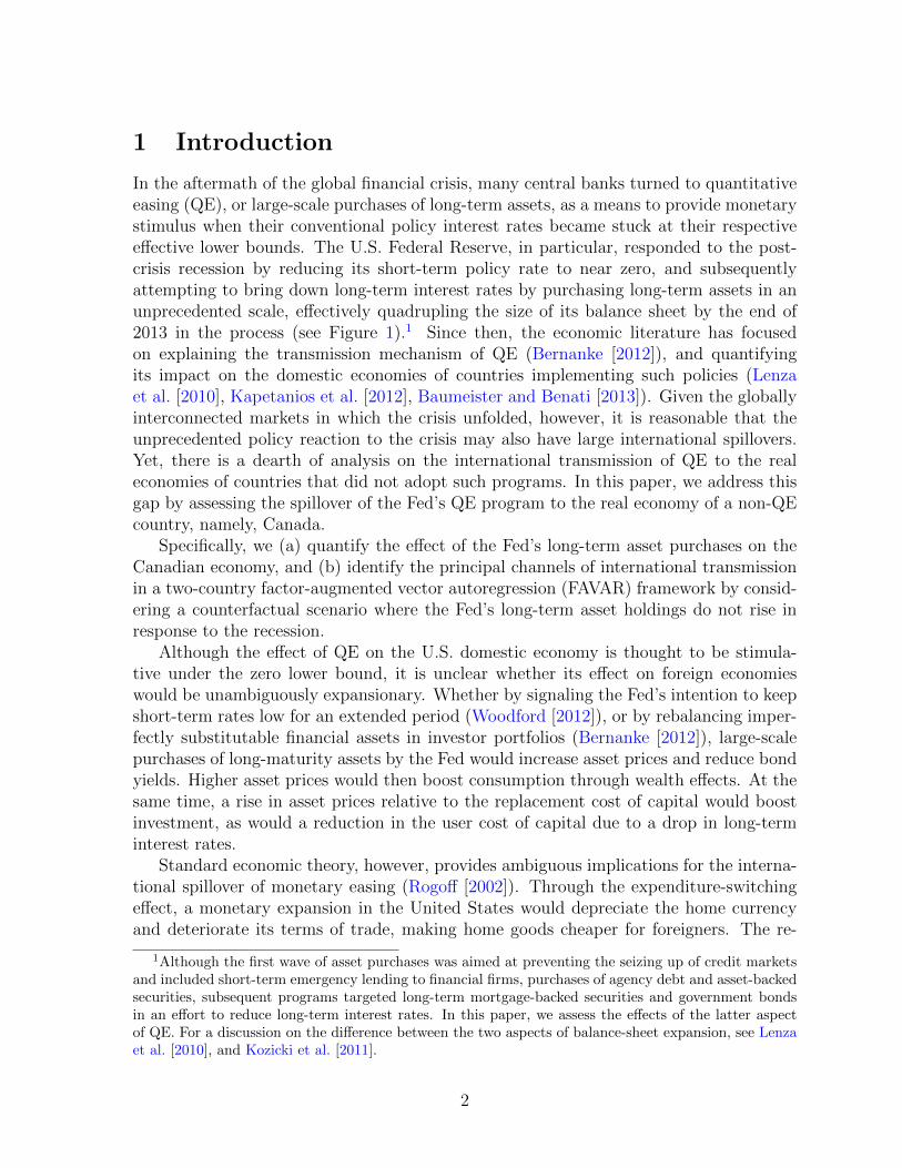
In the aftermath of the global financial crisis, many central banks turned to quantitativeeasing (QE), or large-scale purchases of long-term assets, as a means to provide monetarystimulus when their conventional policy interest rates became stuck at their respectiveeffective lower bounds. The U.S. Federal Reserve, in particular, responded to the post-crisis recession by reducing its short-term policy rate to near zero, and subsequentlyattempting to bring down long-term interest rates by purchasing long-term assets in anunprecedented scale, effectively quadrupling the size of its balance sheet by the end of2013 in the process (see Figure 1).1 Since then, the economic literature has focusedon explaining the transmission mechanism of QE (Bernanke [2012]), and quantifyingits impact on the domestic economies of countries implementing such policies (Lenzaet al. [2010], Kapetanios et al. [2012], Baumeister and Benati [2013]). Given the globallyinterconnected markets in which the crisis unfolded, however, it is reasonable that theunprecedented policy reaction to the crisis may also have large international spillovers.Yet, there is a dearth of analysis on the international transmission of QE to the realeconomies of countries that did not adopt such programs. In this paper, we address thisgap by assessing the spillover of the Fed’s QE program to the real economy of a non-QEcountry, namely, Canada.

Specifically, we (a) quantify the effect of the Fed’s long-term asset purchases on theCanadian economy, and (b) identify the principal channels of international transmissionin a two-country factor-augmented vector autoregression (FAVAR) framework by consid-ering a counterfactual scenario where the Fed’s long-term asset holdings do not rise inresponse to the recession.

Although the effect of QE on the U.S. domestic economy is thought to be stimula-tive under the zero lower bound, it is unclear whether its effect on foreign economieswould be unambiguously expansionary. Whether by signaling the Fed’s intention to keepshort-term rates low for an extended period (Woodford [2012]), or by rebalancing imper-fectly substitutable financial assets in investor portfolios (Bernanke [2012]), large-scalepurchases of long-maturity assets by the Fed would increase asset prices and reduce bondyields. Higher asset prices would then boost consumption through wealth effects. At thesame time, a rise in asset prices relative to the replacement cost of capital would boostinvestment, as would a reduction in the user cost of capital due to a drop in long-terminterest rates.

Standard economic theory, however, provides ambiguous implications for the interna-tional spillover of monetary easing (Rogoff [2002]). Through the expenditure-switchingeffect, a monetary expansion in the United States would depreciate the home currencyand deteriorate its terms of trade, making home goods cheaper for foreigners. The re-

1Although the first wave of asset purchases was aimed at preventing the seizing up of credit marketsand included short-term emergency lending to financial firms, purchases of agency debt and asset-backedsecurities, subsequent programs targeted long-term mortgage-backed securities and government bondsin an effort to reduce long-term interest rates. In this paper, we assess the effects of the latter aspectof QE. For a discussion on the difference between the two aspects of balance-sheet expansion, see Lenzaet al. [2010], and Kozicki et al. [2011].

2

sulting increase in home country net exports would then detract from the real output ofthe foreign economy. The income-absorption effect, on the other hand, implies that aslong as expansionary monetary policy in the home country drives up domestic income,home demand for imports would rise, boosting the economy of foreign exporters. Finally,in the presence of global financial market integration, any increase in asset prices andreductions in yields in the domestic financial market resulting from QE may be reflectedby similar movements in corresponding foreign financial market variables,2 which in turnwould boost foreign consumption and investment through the same mechanism as itdoes in the domestic case. Therefore, whether Canada benefits from the U.S. expansionthrough QE depends on which of these effects dominate, and is an empirical questionthat we attempt to answer here.

Our interest in identifying the international transmission channels of QE makesFAVAR (Bernanke et al. [2005], Boivin and Giannoni [2007], Charnavoki and Dolado[2014]) the appropriate framework to consider, since it allows us to simultaneously assessthe dynamic interactions between a large number of financial and real variables.

We choose Canada as an important case to highlight international transmission chan-nels for a number of reasons. First, its strong trade and financial ties with the UnitedStates makes it reasonable to expect spillovers to be strong and easily observable. Sec-ond, the Bank of Canada did not implement QE, since the pre-crisis resilience of theCanadian financial sector prevented severe financial contagion during the crisis.3 Figure1 shows, however, that despite virtually no change in the amount of long-term assets inthe Bank of Canada’s balance-sheet holdings,4 long-term spreads in Canada fell at thesame time as its U.S. counterpart. Third, Canada is a small open economy with a floatingexchange rate, with a long tradition of independent monetary policy, and availability ofquality data. The latter is of particular practical importance when considering a FAVARanalysis. Finally, Canada is also a commodity exporter, allowing for a richer explorationof possible spillover channels of QE. For example, even when the income-absorption effectdominates in the United States, higher import demand for Canadian energy products maydrive up the Canadian exchange rate, putting the non-energy sectors at a disadvantagefrom an export price point of view.5

2Indeed, Fratzscher et al. [2013] find that QE boosted equity prices worldwide, including in Canada,while Bauer and Neely [2012] show that long-term Canadian yields decreased following U.S. large-scaleasset purchase announcements.

3Note that Canada provided direct qualitative signals on the future path of short-term rates throughforward guidance statements, as did the United States (Fay and Gravelle [2008]). Moreover, the Bankof Canada provided term-liquidity facilities to financial market participants to stabilize the financialsystem and limit the repercussions of the crisis to the Canadian economy (Zorn et al. [2009]).

4The increase in the other-asset category seen from 2011 onwards reflects the Canadian federalgovernment’s debt management strategy. Specifically, in the 2011 federal budget, the governmentdecided to hold prudential assets in the form of cash and short-term treasuries that would allowit to operate for one month in case its regular access to financial markets were hindered. For de-tails, see the government’s prudential liquidity-management plan delineated in the budget document,http://www.budget.gc.ca/2011/plan/anx2-eng.html. Taking a purely monetarist approach, how-ever, one might interpret the rise in the total assets of the Bank of Canada’s balance sheet as a monetaryexpansion (Gambacorta et al. [2012]).

5Using a FAVAR approach, Charnavoki and Dolado [2014] find that a higher exchange due to high

3

Since the beginning of the foray into unconventional policy, a number of studies haveattempted to quantify the effects of QE on domestic financial markets (Gagnon et al.[2011], Krishnamurthy and Vissing-Jorgensen [2011]), and domestic real economies ofcountries conducting such policies (cf. Lenza et al. [2010] for an analysis on the euroarea, Kapetanios et al. [2012] for the United Kingdom, Baumeister and Benati [2013] forthe United States and United Kingdom, Schenkelberg and Watzka [2013] for Japan, andGambacorta et al. [2012] for an international comparison), as well as on the spillovers ofQE to international financial markets (Fratzscher et al. [2013], Bauer and Neely [2012]).To the best of our knowledge, this is the only paper that attempts to assess the effectsof international spillovers of QE on the real economy. In this sense, it complements theliterature on the real spillovers of conventional monetary policy (Kim [2001], Kazi et al.[2013]).

Our approach differs from existing studies on the effects of QE in two importantways. First, while earlier studies proxy U.S. policy through its intended, but unobserved,effects on long-term rates, we directly measure policy action through the observableexpansion of the Fed’s balance sheet. With limited information available at the onset ofthe implementation of QE, early papers on the topic take findings from event studies onfinancial market reactions to Fed announcements as given, and construct counterfactualscenarios where the absence of QE is proxied through higher long-term rates.6 We, onthe other hand, measure QE as the Fed’s balance-sheet holdings of long-term assets, andconstruct a counterfactual scenario where these holdings are not increased in reaction tothe great recession. Our measure takes advantage of 19 quarters of observable data, andis agnostic about the effect on long-term rates. Note, however, that we retain the focuson long-term asset purchases, rather than the increase in the monetary base or the totalsize of the Fed’s balance sheet as considered by Gambacorta et al. [2012].7

Second, we estimate a two-country FAVAR with coefficient restrictions which allowsus to study the transmission of U.S. policy through dynamic interactions between a largenumber of financial and real variables, while at the same time restricting U.S. policyfrom being influenced by movements in Canadian economic variables. We believe thisis the appropriate framework for studying relationships between a large country such asthe United States and a small open economy such as Canada (Charnavoki and Dolado

energy prices negatively impacts the non-energy sector output only after a negative energy supply shock,while it positively impacts non-energy sector output following a positive global demand shock. Thisfinding is mirrored by Dorich et al. [2013], who use an estimated dynamic stochastic general-equilibrium(DSGE) framework.

6Looking at financial market reaction within a short time-window of the Fed announcements regardingQE, Gagnon et al. [2011] and Krishnamurthy and Vissing-Jorgensen [2011] suggest that QE loweredlong-term treasury yields by between 30 and 100 basis points. Baumeister and Benati [2013] accordinglyconstruct their counterfactual scenario of a world without QE as one where long-term yields are 100basis points higher. In a similar event study, Joyce et al. [2011] find that QE announcements in theUnited Kingdom reduced long-term government bond rates by 100 basis points. This, in turn, serves asthe basis for the counterfactual scenario considered by Kapetanios et al. [2012].

7Interpreting QE as an increase in the total size of the Fed’s balance sheet or monetary base espousesa purely monetarist view that relies on the structural stability of the money multiplier and the velocityof money (Woodford [2012]).

4

[2014]).We find that the implementation of QE increases U.S. output by about 2.3 percent and

Canadian output by 2.2 percent on average between 2008Q4 and 2013Q3, when comparedwith the no-QE counterfactual scenario. Because of QE, U.S. long-term spreads decline,and asset prices rise, boosting both investment and consumption, though the latter is notstatistically significant. The transmission to Canada occurs mostly through the financialmarket. Although Canada did not implement QE, long-term spreads in Canada fall, andasset prices in the Canadian stock market rise. QE also leads to higher oil prices, animprovement in the Canadian terms of trade and an appreciation of the Canadian nominalexchange rate vis-a-vis the United States, consistent with the commodity currency effectdocumented by Charnavoki and Dolado [2014] and Dorich et al. [2013].

In other words, financial market integration results in Canadian interest rates andasset prices moving in the same direction as those in the United States following theimplementation of QE. Along with the effects of improved terms of trade, spillovers fromthe financial channel bolster the domestic Canadian economy, driving up Canadian de-mand for imports, while the appreciation of the Canadian dollar makes imports cheaper.As a consequence, net exports fall, despite the fact that Canadian exports increase inmost product categories, consistent with a stronger U.S. economy. Our finding that thefinancial channel dominates the trade channel in transmitting positive spillovers from aU.S. monetary expansion is consistent with the transmission of conventional monetarypolicy documented by Kim [2001] using a small structural vector autoregression.

The rest of the paper is organized as follows. Section 2 describes the two-countryFAVAR set-up, as well as the data and estimation process. Section 3 describes thecounterfactual set-up and the results of the exercise for both aggregate real and financialvariables, as well as some disaggregated variables. We provide some robustness analysisin section 4, including a qualitative look at the transmission mechanism for a conventionalmonetary policy shock to the U.S. policy rate. Section 5 concludes.

2 Empirical Framework

We choose a FAVAR approach (Bernanke et al. [2005] and Boivin and Giannoni [2007])to assess the different international transmission channels of QE. This is the appropriateframework to consider, since it allows us to simultaneously compare the effect of QE on abroad set of financial and real variables from Canada and the United States, while takinginto account the dynamic interactions between them. We explain our empirical set-up,describe the data and discuss the estimation method below.

2.1 Empirical model

Our FAVAR specification contains two country-specific blocks. Following Charnavokiand Dolado [2014], we impose two restrictions to reflect the small open-economy natureof Canada. First, by imposing block-zero restrictions on the VAR coefficients, we ensurethat movements in Canadian factors do not influence movements in U.S. factors. Second,

5

by specifying that Canadian time series load onto both U.S. and Canadian factors, weallow for a strong co-movement between real and financial variables of both countries,while keeping unobserved factors orthogonal to each other.

The one-directional nature of the relationship between these two countries inherent inour modeling choice is motivated by the following observations from international tradeand financial flow data. First, Canada is highly dependent on the United States forits international trade, while the reverse is not true. On average, 84 percent of totalCanadian exports between 2000 and 2007 were destined for the United States. However,this accounted for only 17 percent of total U.S. imports. Table 1 shows that this disparityis true for Canadian imports as well, and holds across all product categories. Internationalfinancial flows between the two countries show a similar pattern. Table 2 shows that 47percent of Canadian portfolio and direct investments abroad are in the United States,while almost 60 percent of foreign direct and portfolio investments in Canada come fromthe United States. In particular, about 80 percent of foreign investments in Canadianequity are held by U.S. investors. Finally, Table 3 shows that both financial markets andreal economies of the two countries are strongly and persistently correlated in businesscycle frequencies. This suggests that the Canadian economy is highly responsive tomovements in U.S. economic and policy variables, while the reverse may not be true.This is reflected in our empirical framework described below.

The first block in our FAVAR model contains a vector of unobservable factors, FUS,Ft ,

that summarizes information about the U.S. economy, and a vector of observable policyvariables, YUS

t , that summarizes the U.S. monetary policy stance. FUSt = (FUS,F

t , YUSt ).

In our case, the policy variables are the effective federal funds rate and our measure ofQE – total long-term asset holdings in the Fed’s balance sheet. The second block consistsof Canada-specific unobservable factors, FCA

t , that are orthogonal to the U.S. factors.The U.S. and Canadian data load onto the factors as follows:[

XUSt

XCAt

]=

[ΛUS

US 0ΛCA

US ΛCACA

] [FUS

t

FCAt

]+

[uUSt

uCAt

], (1)

where XUSt and XCA

t are data for the U.S. and Canadian economies, ΛjUS = (Λj

US,F ΛjUS,Y )

are the loading matrices corresponding to the unobservable and observable U.S. factors,and ΛCA

CA denotes the loading matrix for the Canadian factors that are orthogonal to theU.S. ones. As we can see, the Canadian data load onto both U.S. and Canada-specificfactors. uUS

t and uCAt are vectors of idiosyncratic disturbances.

We model the dynamics of the factors as a restricted VAR (see, e.g., Charnavoki andDolado [2014]): [

FUSt

FCAt

]=

[b11(L) 0b21(L) b22(L)

] [FUS

t−1

FCAt−1

]+ et, (2)

where bij(L) are lag polynomials of finite order p and et denotes the reduced-form residu-als. The block of zeros in the coefficient matrix prevents movements in Canadian factorsto influence those in the United States. As argued above, we believe that this restrictionadequately captures the small open-economy nature of Canada. Relaxing this restriction,however, does not alter our main findings presented below. Combining equations (1) and

6

(2), one-step-ahead forecasts for each series contained in the data set can be obtainedfrom the following equation:[

XUSt

XCAt

]=

[ΛUS

US 0ΛCA

US ΛCACA

] [b11(L) 0b21(L) b22(L)

] [FUS

t−1

FCAt−1

]+ εt. (3)

2.2 Data

We use quarterly data from 122 U.S. and 149 Canadian series ranging from 1983Q1through 2013Q3. The start date is restricted by the availability of Canadian disaggre-gated data. The U.S. series include real data from national income, industrial production,employment by industry, as well as data on housing starts and sales, manufacturers’ or-ders and inventory, and a number of different price indexes. Movements in the financialsector are captured through stock prices, nominal and real exchange rates, interest ratesof varying maturity, bond prices, monetary aggregates, and commercial bank balance-sheet and lending conditions. We also include confidence indexes from the ConferenceBoard and University of Michigan surveys on business sentiment. The QE variable rep-resents the Federal Reserve’s balance-sheet holdings of mortgage-backed securities andtreasury bonds with maturities of more than five years. A more detailed discussion onthe choice of this variable is provided in section 3 while describing the counterfactualset-up.

The Canadian series include real data on national accounts, Canadian exports andimports by product and by regional destination, flows from the balance of paymentsaccount, and industry-level GDP and employment. We also include Canadian houseprices and housing starts, and a number of relative price and oil price indexes. Movementin the financial sector is captured through the Toronto Stock Exchange (TSX) price index,nominal and trade-weighted real exchange rates, interest rates of various maturities, aswell as balance-sheet conditions from commercial banks and private industry. We captureCanadian business confidence by the Conference Board confidence index.

Most of our data series, both U.S. and Canadian, are downloaded via HAVER ana-lytics. We construct the industry-level GDP for Canada by combining information fromtables 379-0027 and 379-0031 from the Canadian Socioeconomic Information Manage-ment (CANSIM) database maintained by Statistics Canada.8 The series are transformedto induce stationarity, and standardized before estimation. For the benchmark case pre-sented in section 3.2, we transform our measure of QE by taking differences in levels, andconsider differences in logs in section 4. The appendix provides detailed descriptions,sources and transformation codes for all series considered.

8Statistics Canada discontinued table 379-0027 in 2012Q4, where real industry-level GDP is measuredin 2002 Canadian dollars, and replaced it with table 379-0031, where data were measured in 2007 dollarsand start in 1997Q1. We construct our GDP series by taking data from the latter table, and growingthem out backwards using the growth rate of corresponding variables from the former table.

7

2.3 Estimation

Following Bernanke et al. [2005], we estimate the FAVAR in two steps. First, the unob-served factors FUS,F

t and FCAt are estimated through principal components from our data

sets XUSt and XCA

t . Second, both unobserved and observed policy variables are then castinto a restricted VAR model.

The unobservable U.S. factors are rotated to be orthogonal to the observed policyvariables as follows. First, we start by extracting KUS factors from the U.S. data setXUS

t as the largest KUS principal components. We then extract the same number offactors from a subset of our data set that contain variables which do not respond topolicy changes contemporaneously, i.e., slow-moving variables. The full set of factorsare then regressed on the set of slow-moving factors and the set of fast-moving policyvariables, YUS

t . The final set of factors, FUS,Ft , are estimated as a rotation of the original

factors that are orthogonal to YUSt .9

We allow Canadian data, XCAt , to load onto both U.S. and Canadian factors, with

loading matrices ΛCAUS and ΛCA

CA, respectively. We estimate the Canadian factors followingthe iterative procedure employed by Charnavoki and Dolado [2014] in order to control forthe effect of the U.S. factors in the Canadian block. Again, we start by extracting KCA

factors from the Canadian data set as the largest KCA principal components. Given thisinitial estimate of the Canadian factors, F

CA(0)t , we iterate through the following steps

until convergence is achieved:

1. Regress XCAt on F

CA(j)t and the estimates of the U.S. factors, FUS

t =[FUS,F

t ,YUSt

],

to obtain ΛCA(j)US .

2. Calculate XCA(j)t = XCA

t − ΛCA(j)US FUS

t .

3. Obtain FCA(j+1)t as the first KCA principal components of X

CA(j)t .

4. Return to step 1. The algorithm stops when the difference between FCA(j+1)t and

FCA(j)t is sufficiently small.

Different versions of the Bai and Ng [2002] criteria suggest between six and ten factorsfor the U.S. block and four to eight factors for the Canadian block. We choose six factorsfor the U.S. block (including the policy variables) and four factors for the Canadian block.Our main message below, however, is robust to any combination of four to ten factors.Using these factors, we estimate equation (2) via restricted ordinary least squares toincorporate the block-zero restriction. We choose only one lag for the VAR to take intoaccount our relatively small sample size.

3 International Transmission of QE

Using the empirical set-up described above, we estimate the effect of QE as the differ-ence between two conditional forecasts: one corresponding to the policy scenario, where

9See Bernanke et al. [2005] for details.

8

the Fed’s long-term asset holdings follow the path observed in data, and the other, thecounterfactual no-policy scenario, where the Fed’s holding of long-term assets does notincrease in response to the great recession. In this section, we first describe our counter-factual set-up, and then discuss the results of our analysis.

3.1 Counterfactual set-up

Although the Federal Reserve announced purchases of mortgage-backed and long-termtreasury securities in a staggered manner since the beginning of the financial crisis,10

actual purchases occurred gradually. Figure 1 shows the rise in long-term asset holdings(holdings of mortgage-backed securities and treasury securities of maturity higher thanfive years) in the Fed balance sheet, along with the policy rate and the 10-year treasuryyield.

For our counterfactual, we construct a no-policy scenario where this increase in long-term asset holdings does not occur. We therefore espouse a view that anticipated in-creases in long-term asset holdings have an effect on the economy. We believe that thisview is somewhere between Gambacorta et al. [2012], who focus on an unanticipatedincrease in the Fed’s balance sheet, and Woodford [2012], who considers that the an-nouncements themselves contain all relevant information about the Fed’s policy actions.In our benchmark case, we generate an unconditional forecast of the Fed’s long-termasset holdings from equation (2) using pre-recession values of the factors. This givesus a path for the QE variable that is consistent with pre-recession dynamics, but onethat does not increase in response to the recession. Our no-policy counterfactual is thengenerated as the expected value of our variables of interest conditional upon this counter-factual path of the Fed’s asset holdings. This approach is similar to Lenza et al. [2010].11

We also consider an alternative scenario where the QE variable is projected using itspre-recession trend growth rate, and find similar results as our benchmark case. Thebenchmark conditional forecasts for the policy and the no-policy scenarios are calculatedas follows.

1. Policy scenario: Using a full-sample estimate of equations (1) and (2), producea forecast from 2008Q4 until 2013Q3, conditional on the actual path of both the

10In November 2008, the Federal Reserve announced purchases of $600 billion worth of mortgage-backed securities. By March 2009, the Fed’s holdings of bank debt, mortgage-backed securities andtreasury notes reached $1.75 trillion. Purchases of long-term treasury securities worth $600 billion wereannounced in November 2010, and a rebalancing of the Fed’s portfolio away from short-term and towardlong-term treasury securities worth $400 billion was announced in September 2011. In September 2012,the Fed announced purchases of mortgage-backed securities worth $40 billion per month, and renewalof the portfolio rebalancing scheme toward long-term securities. In December 2012, the Fed increasedpurchases of mortgage-backed securities from $40 to $85 billion per month. Finally, in June 2013, theFed announced a “tapering” of the Fed’s asset purchases.

11In contrast, Kapetanios et al. [2012] and Baumeister and Benati [2013] consider a counterfactual setof coincident structural shocks, identified through sign restrictions, that move spreads a certain amounthigher than observed, while keeping the federal funds rate at the zero lower bound. By conditioning ona particular path of a policy variable, we are spared from imposing a structural interpretation on the setof shocks that represent the Fed’s observed policy action.

9

QE variable x∗,QEt and the effective federal funds rate, x∗,FF

t :

XT+h = ET

(XT+h|B(L),F0...FT+h, x

∗,QET+h , x

∗,FFT+h

)for T + h = 2008Q4...2013Q3. This is the policy scenario.

2. No-policy scenario: To produce forecasts under the no-policy scenario, first gen-erate a counterfactual path of the QE variable. Second, obtain conditional forecastsusing this path and a full sample estimate of equations (1) and (2).

(a) We generate the counterfactual path of the QE variables in two alternativeways.

i. Estimate the restricted regression (Equation (2)) using estimated factorsthrough 2008Q3:

Ft = B1(L)Ft−1 + et

t = 1983Q1...2008Q3.

Produce an unconditional forecast for the remainder of the sample, andsave the path of the QE variable xQE

T+h ∈ XT+h = ET

(XT+h|B1(L),F0...FT+h

)for T + h = 2008Q4...2013Q3. This gives us the counterfactual path ofthe QE variable, which is used as our benchmark.

ii. Construct a counterfactual path for the QE variable where it grows accord-ing to a linear and quadratic pre-QE time trend. That is, to obtain a pathfor T + h = 2008Q4...2013Q3 apply the trend for t = 1983Q1...2008Q3.This gives us the counterfactual path of the QE variable, which is usedfor robustness.

(b) Construct a counterfactual forecast from 2008Q4 until 2013Q3, conditional onthe actual path of the effective federal funds rate, x∗,FF

T+h , and the counterfactual

path of the QE variable, xQET+h, constructed above:

XT+h = ET

(XT+h|B,F0...FT+h, x

QET+h, x

∗,FFT+h

)for T + h = 2008Q4...2013Q3. This is the no-policy counterfactual scenario.

3. The difference between XT+h and XT+h is then the effect of QE.

Note that, while we directly measure policy action through 19 quarters of observ-able expansion of the Fed’s balance sheet, we remain agnostic about the quantitativeeffect (or, even, the direction of change) of QE on long-term rates. In contrast, earlystudies estimating the effect of QE proxy central bank policy through its intended, butunobserved, effect on long-term rates. Gagnon et al. [2011] and Krishnamurthy andVissing-Jorgensen [2011] use event-study methods on financial markets to estimate thatearly Fed announcements related to QE reduced long-term yields by 30 to 107 basis points

10

(bps). With limited information available at the onset of the implementation of this novelpolicy paradigm, early studies on the effect of QE take these estimates of announcementeffects on long-term yields as given, and construct counterfactual scenarios where, in theabsence of QE, long-term spreads are higher by the same amount (Baumeister and Benati[2013], Kapetanios et al. [2012]).

3.2 Results

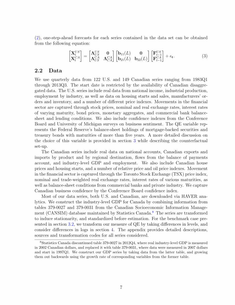
Figures 2 and 3 show the effect of QE for a key set of variables for the United States andCanada, respectively. The solid line represents the difference between the two conditionalpoint forecasts, and the dashed lines show the 68 percent residual bootstrap bands fromthe counterfactual exercise described above. Note that although these figures resembletraditional impulse responses, they are not so. Instead, they represent the differencebetween the policy scenario and the no-policy scenario at each quarter of the forecasthorizon. When noted, results are expressed in percentage difference from the no-policyscenario.

A number of key results emerge from our exercise. First, as Figure 2 suggests, QEboosts domestic U.S. GDP by lowering long-term spreads. Compared to the counterfac-tual scenario, on average between 2008Q4 and 2013Q3, the increase in long-term assetholdings in the Fed balance sheet reduces the 10-year treasury spread by 82 bps, andincreases GDP by 2.3 percent and the personal consumption expenditure price index by0.5 percent. Note that our result of a positive impact of QE on U.S. GDP is not derivedfrom an explicit assumption of a reduced long-term spread. Rather, the latter arises asan endogenous response to an increase in the Fed’s long-term asset holdings. The mag-nitude of decline in long-term spreads is comparable to Neely [2010], Krishnamurthy andVissing-Jorgensen [2011], and Bauer and Neely [2012], who find, using different empiricaltechniques, that long-term treasury yields fell by 88, 107, and 123 bps, respectively, dueto the Fed’s 2009 asset purchases, and to Gagnon et al. [2011], who find that the samepurchases resulted in a reduction in the 10-year term premium by 30 to 100 bps. Oureffect on GDP is also in the same order of magnitude as Chung et al. [2012], who findthat a cumulative 70 bps drop in the term premium due to QE resulted in real GDPbeing higher by 3 percentage points by early 2012. Moreover, the higher personal con-sumption price under the QE scenario than under the no-policy scenario suggests thatour counterfactual exercise does not generate a price puzzle for QE that is often foundin the literature on conventional monetary policy shocks.

The domestic transmission of QE occurs largely along the lines explained by Bernanke[2012]. Asset prices (the S&P 500 index), consumer confidence (Conference Board in-dicator), the banking sector’s willingness to lend (Federal Reserve’s senior loan officersurvey), and commercial and industrial loans all increase, while corporate spreads (BAA- AAA) decline. This raises U.S. investment, and, to a lesser extent, consumption.12

12To put our quantitative results into better perspective, consider the following two examples: in2013Q3, real investment and the S&P price index in our QE scenario are estimated to be 38 and 162percent higher than in our no-policy scenario, respectively. Data show that in 2013Q3, investment was

11

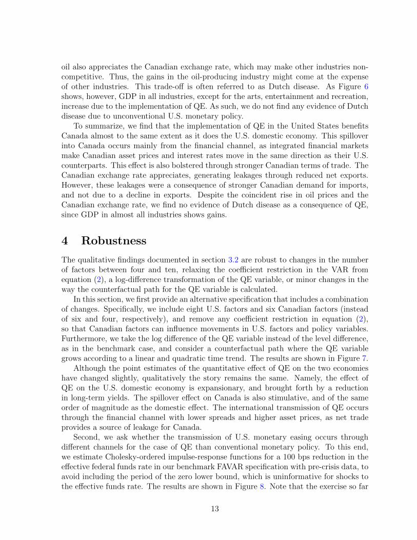
Second, Figure 3 shows that the spillover effect of QE on Canada is positive, and of thesame order of magnitude as in the United States. In the financial market, the increase inthe Fed’s long-term asset holdings reduces the 10-year Canadian government bond spreadby 30 bps on average between 2008Q4 and 2013Q3, compared to the counterfactual. Inthe goods market, Canadian GDP increases by 2.2 percent, and the consumer price indexby 0.5 percent, on average in the same period. In comparison, Bauer and Neely [2012]find that the 2009 asset purchases by the Fed reduced Canadian 10-year yields by 66 bps.

Third, the transmission of QE to Canada occurs mainly through financial channels.Due to strong financial integration, the Canadian corporate spread (Canadian 3-monthcorporate bond yield - Canadian 3-month government bond yield) falls, while both Cana-dian asset prices (TSX index), and consumer confidence (Conference Board index) risealongside their U.S. counterparts. Consequently, both Canadian consumption and in-vestment increase. Our finding that QE in the U.S. transmits to Canada through thefinancial rather than the trade channel complements a similar finding by Kim [2001] fora conventional monetary policy shock.

Importantly, compared with the no-policy scenario, QE leads to higher oil prices(Brent prices are shown in Figure 3), an improvement in the Canadian terms of tradeand an appreciation of the Canadian nominal exchange rate vis-a-vis the United States.This is consistent with the commodity currency effect documented by Charnavoki andDolado [2014] and Dorich et al. [2013]. Positive spillovers from improved terms of tradebolster Canadian income and wealth, and work in the same direction as the spilloversfrom the financial channel in raising Canadian consumption and investment.

Finally, net exports fall. However, this is due to higher imports from a comparativelystronger Canadian domestic demand, rather than lower exports to the United States.Looking closer at net exports, however, we find two important trends that contradicta purely expenditure-switching view. First, as we see in Figure 3, although Canadianglobal net exports decline compared to the counterfactual, net exports destined to theUnited States increase, or at least stay the same, during that period, suggesting that thedecline in net exports is due to trade with the rest of the world. Second, Figures 4 and 5show that the decline in Canadian net exports is due not to a fall in exports, but ratherto stronger imports in almost all product categories.

In other words, financial market integration results in Canadian interest rates andasset prices moving in the same direction as those in the United States following theimplementation of QE. Along with the effects of improved terms of trade, spillovers fromthe financial channel bolster the domestic Canadian economy, driving up Canadian de-mand for imports, while the appreciation of the Canadian dollar makes imports cheaper.As a consequence, net exports fall, despite the fact that Canadian exports increase inmost product categories, consistent with a stronger U.S. economy.

Finally, Figure 6 shows the impact of QE on Canadian GDP by industry. As acommodity-exporting country, Canada generally benefits from a rise in global oil prices.At the same time, the commodity currency effect implies that increased demand for

45.6 percent and the S&P index was 107 percent higher than their recessionary troughs, which occurredin 2009Q3 and 2009Q1, respectively.

12

oil also appreciates the Canadian exchange rate, which may make other industries non-competitive. Thus, the gains in the oil-producing industry might come at the expenseof other industries. This trade-off is often referred to as Dutch disease. As Figure 6shows, however, GDP in all industries, except for the arts, entertainment and recreation,increase due to the implementation of QE. As such, we do not find any evidence of Dutchdisease due to unconventional U.S. monetary policy.

To summarize, we find that the implementation of QE in the United States benefitsCanada almost to the same extent as it does the U.S. domestic economy. This spilloverinto Canada occurs mainly from the financial channel, as integrated financial marketsmake Canadian asset prices and interest rates move in the same direction as their U.S.counterparts. This effect is also bolstered through stronger Canadian terms of trade. TheCanadian exchange rate appreciates, generating leakages through reduced net exports.However, these leakages were a consequence of stronger Canadian demand for imports,and not due to a decline in exports. Despite the coincident rise in oil prices and theCanadian exchange rate, we find no evidence of Dutch disease as a consequence of QE,since GDP in almost all industries shows gains.

4 Robustness

The qualitative findings documented in section 3.2 are robust to changes in the numberof factors between four and ten, relaxing the coefficient restriction in the VAR fromequation (2), a log-difference transformation of the QE variable, or minor changes in theway the counterfactual path for the QE variable is calculated.

In this section, we first provide an alternative specification that includes a combinationof changes. Specifically, we include eight U.S. factors and six Canadian factors (insteadof six and four, respectively), and remove any coefficient restriction in equation (2),so that Canadian factors can influence movements in U.S. factors and policy variables.Furthermore, we take the log difference of the QE variable instead of the level difference,as in the benchmark case, and consider a counterfactual path where the QE variablegrows according to a linear and quadratic time trend. The results are shown in Figure 7.

Although the point estimates of the quantitative effect of QE on the two economieshave changed slightly, qualitatively the story remains the same. Namely, the effect ofQE on the U.S. domestic economy is expansionary, and brought forth by a reductionin long-term yields. The spillover effect on Canada is also stimulative, and of the sameorder of magnitude as the domestic effect. The international transmission of QE occursthrough the financial channel with lower spreads and higher asset prices, as net tradeprovides a source of leakage for Canada.

Second, we ask whether the transmission of U.S. monetary easing occurs throughdifferent channels for the case of QE than conventional monetary policy. To this end,we estimate Cholesky-ordered impulse-response functions for a 100 bps reduction in theeffective federal funds rate in our benchmark FAVAR specification with pre-crisis data, toavoid including the period of the zero lower bound, which is uninformative for shocks tothe effective funds rate. The results are shown in Figure 8. Note that the exercise so far

13

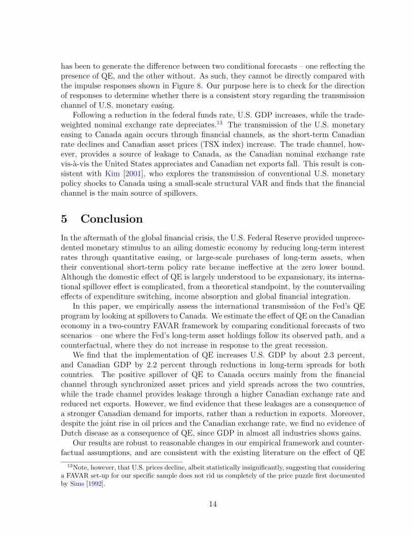
has been to generate the difference between two conditional forecasts – one reflecting thepresence of QE, and the other without. As such, they cannot be directly compared withthe impulse responses shown in Figure 8. Our purpose here is to check for the directionof responses to determine whether there is a consistent story regarding the transmissionchannel of U.S. monetary easing.

Following a reduction in the federal funds rate, U.S. GDP increases, while the trade-weighted nominal exchange rate depreciates.13 The transmission of the U.S. monetaryeasing to Canada again occurs through financial channels, as the short-term Canadianrate declines and Canadian asset prices (TSX index) increase. The trade channel, how-ever, provides a source of leakage to Canada, as the Canadian nominal exchange ratevis-a-vis the United States appreciates and Canadian net exports fall. This result is con-sistent with Kim [2001], who explores the transmission of conventional U.S. monetarypolicy shocks to Canada using a small-scale structural VAR and finds that the financialchannel is the main source of spillovers.

5 Conclusion

In the aftermath of the global financial crisis, the U.S. Federal Reserve provided unprece-dented monetary stimulus to an ailing domestic economy by reducing long-term interestrates through quantitative easing, or large-scale purchases of long-term assets, whentheir conventional short-term policy rate became ineffective at the zero lower bound.Although the domestic effect of QE is largely understood to be expansionary, its interna-tional spillover effect is complicated, from a theoretical standpoint, by the countervailingeffects of expenditure switching, income absorption and global financial integration.

In this paper, we empirically assess the international transmission of the Fed’s QEprogram by looking at spillovers to Canada. We estimate the effect of QE on the Canadianeconomy in a two-country FAVAR framework by comparing conditional forecasts of twoscenarios – one where the Fed’s long-term asset holdings follow its observed path, and acounterfactual, where they do not increase in response to the great recession.

We find that the implementation of QE increases U.S. GDP by about 2.3 percent,and Canadian GDP by 2.2 percent through reductions in long-term spreads for bothcountries. The positive spillover of QE to Canada occurs mainly from the financialchannel through synchronized asset prices and yield spreads across the two countries,while the trade channel provides leakage through a higher Canadian exchange rate andreduced net exports. However, we find evidence that these leakages are a consequence ofa stronger Canadian demand for imports, rather than a reduction in exports. Moreover,despite the joint rise in oil prices and the Canadian exchange rate, we find no evidence ofDutch disease as a consequence of QE, since GDP in almost all industries shows gains.

Our results are robust to reasonable changes in our empirical framework and counter-factual assumptions, and are consistent with the existing literature on the effect of QE

13Note, however, that U.S. prices decline, albeit statistically insignificantly, suggesting that consideringa FAVAR set-up for our specific sample does not rid us completely of the price puzzle first documentedby Sims [1992].

14

on the U.S. domestic economy and global financial markets, as well as the literature onthe international transmission of conventional U.S. monetary stimulus.

References

Jushan Bai and Serena Ng. Determining the number of factors in approximate factormodels. Econometrica, 70(1):191–221, 2002.

Michael D. Bauer and Christopher J. Neely. International channels of the Feds uncon-ventional monetary policy. Technical report, 2012.

Christiane Baumeister and Luca Benati. Unconventional monetary policy and the greatrecession: Estimating the macroeconomic effects of a spread compression at the zerolower bound. International Journal of Central Banking, 9(2):165–212, June 2013.

Ben Bernanke, Jean Boivin, and Piotr S. Eliasz. Measuring the effects of monetary policy:A factor-augmented vector autoregressive (FAVAR) approach. Quarterly Journal ofEconomics, 120(1):387–422, January 2005.

Ben S. Bernanke. Monetary Policy since the Onset of the Crisis: a speech at the FederalReserve Bank of Kansas City Economic Symposium, Jackson Hole, Wyoming, August31, 2012. (645), August 2012. URL http://ideas.repec.org/p/fip/fedgsq/645.

html.

Jean Boivin and Marc P. Giannoni. Global forces and monetary policy effectiveness.In International Dimensions of Monetary Policy, NBER Chapters, pages 429–478.National Bureau of Economic Research, Inc, July 2007. URL http://ideas.repec.

org/h/nbr/nberch/0515.html.

Valery Charnavoki and Juan J. Dolado. The Effects of Global Shocks on SmallCommodity-Exporting Economies: Lessons from Canada. American Economic Jour-nal: Macroeconomics, 6(2):207–37, April 2014. URL http://ideas.repec.org/a/

aea/aejmac/v6y2014i2p207-37.html.

Hess Chung, JeanPhilippe Laforte, David Reifschneider, and John C. Williams. Have WeUnderestimated the Likelihood and Severity of Zero Lower Bound Events? Journal ofMoney, Credit and Banking, 44:47–82, 02 2012. URL http://ideas.repec.org/a/

mcb/jmoncb/v44y2012ip47-82.html.

Jose Dorich, Michael K. Johnston, Rhys R. Mendes, Stephen Murchison, and Yang Zhang.ToTEM II: An Updated Version of the Bank of Canada’s Quarterly Projection Model.Technical report, 2013.

Christine Fay and Toni Gravelle. The Market Impact of Forward-LookingPolicy Statements: Transparency vs. Predictability. Bank of Canada Re-view, 2008(Winter):27–36, 2008. URL http://ideas.repec.org/a/bca/bcarev/

v2009y2009iwinter08-09p27-36.html.

15

Marcel Fratzscher, Marco Lo Duca, and Roland Straub. On the international spilloversof US quantitative easing. Working Paper Series 1557, European Central Bank, June2013. URL http://ideas.repec.org/p/ecb/ecbwps/20131557.html.

Joseph Gagnon, Matthew Raskin, Julie Remache, and Brian Sack. Large-scale assetpurchases by the Federal Reserve: did they work? Economic Policy Review, (May):41–59, 2011. URL http://ideas.repec.org/a/fip/fednep/y2011imayp41-59nv.

17no.1.html.

Leonardo Gambacorta, Boris Hofmann, and Gert Peersman. The Effectiveness of Un-conventional Monetary Policy at the Zero Lower Bound: A Cross-Country Analysis.BIS Working Papers 384, Bank for International Settlements, August 2012. URLhttp://ideas.repec.org/p/bis/biswps/384.html.

Michael A. S. Joyce, Ana Lasaosa, Ibrahim Stevens, and Matthew Tong. The FinancialMarket Impact of Quantitative Easing in the United Kingdom. International Journalof Central Banking, 7(3):113–161, September 2011. URL http://ideas.repec.org/

a/ijc/ijcjou/y2011q3a5.html.

George Kapetanios, Haroon Mumtaz, Ibrahim Stevens, and Konstantinos Theodoridis.Assessing the economywide effects of quantitative easing. Economic Journal, 122(564):F316–F347, November 2012.

Irfan Akbar Kazi, Hakimzadi Wagan, and Farhan Akbar. The changing internationaltransmission of U.S. monetary policy shocks: Is there evidence of contagion effecton OECD countries. Economic Modelling, 30(C):90–116, 2013. URL http://ideas.

repec.org/a/eee/ecmode/v30y2013icp90-116.html.

Soyoung Kim. International transmission of U.S. monetary policy shocks: Evidencefrom VAR’s. Journal of Monetary Economics, 48(2):339–372, October 2001. URLhttp://ideas.repec.org/a/eee/moneco/v48y2001i2p339-372.html.

Sharon Kozicki, Eric Santor, and Lena Suchanek. Unconventional Monetary Policy:The International Experience with Central Bank Asset Purchases. Bank of CanadaReview, 2011(Spring):13–25, 2011. URL http://ideas.repec.org/a/bca/bcarev/

v2011y2011ispring11p13-25.html.

Arvind Krishnamurthy and Annette Vissing-Jorgensen. The Effects of QuantitativeEasing on Interest Rates: Channels and Implications for Policy. NBER WorkingPapers 17555, National Bureau of Economic Research, Inc, October 2011. URLhttp://ideas.repec.org/p/nbr/nberwo/17555.html.

Michele Lenza, Huw Pill, and Lucrezia Reichlin. Monetary policy in exceptionaltimes. Economic Policy, 25:295–339, 04 2010. URL http://ideas.repec.org/a/

bla/ecpoli/v25y2010ip295-339.html.

16

Christopher J. Neely. The large scale asset purchases had large international effects.Technical report, 2010.

Kenneth Rogoff. Dornbusch’s Overshooting Model After Twenty-Five Years. IMFWorking Papers 02/39, International Monetary Fund, February 2002. URL http:

//ideas.repec.org/p/imf/imfwpa/02-39.html.

Heike Schenkelberg and Sebastian Watzka. Real effects of quantitative easing at the zerolower bound: Structural VAR-based evidence from Japan. Journal of InternationalMoney and Finance, 33(C):327–357, 2013. URL http://ideas.repec.org/a/eee/

jimfin/v33y2013icp327-357.html.

Christopher A. Sims. Interpreting the macroeconomic time series facts: The effectsof monetary policy. European Economic Review, 36(5):975–1000, June 1992. URLhttp://ideas.repec.org/a/eee/eecrev/v36y1992i5p975-1000.html.

Michael Woodford. Methods of policy accommodation at the interest-rate lower bound.Proceedings - Economic Policy Symposium - Jackson Hole, pages 185–288, 2012. URLhttp://ideas.repec.org/a/fip/fedkpr/y2012p185-288.html.

Lorie Zorn, Carolyn Wilkins, and Walter Engert. Bank of Canada LiquidityActions in Response to the Financial Market Turmoil. Bank of Canada Re-view, 2009(Autumn):7–26, 2009. URL http://ideas.repec.org/a/bca/bcarev/

v2009y2009iautumn09p7-26.html.

17

Table 1: Goods trade between Canada and the United States (2000-2007 averages)

% of country’s total exports or imports

Can exports U.S. imports Can imports U.S. exportsto U.S. from Can from U.S. to Can

All goods 83.9 17.3 58.9 22.7Agriculture 45.1 19.2 64.1 13.5Forestry 84.9 55.1 71.7 33.6Oil and gas 98.9 22.8 20.6 22.3Mining (ex. oil and gas) 35.4 25.6 53.4 29.5Consumer goods 77.7 14.7 50.0 25.0Chemicals 85.1 16.5 69.4 20.4Metals and minerals 80.6 20.3 61.0 32.2Machinery 77.7 11.9 61.8 22.5Electronics 76.4 5.0 46.2 15.7Autos 97.3 29.9 77.3 56.0Other transportation 71.9 23.1 56.9 8.7Other goods 82.6 2.5 44.2 15.0

Notes: Calculated based on nominal annual series in CAD (industry breakdown of Canadianexports and imports) and USD (all other values). Percentages of total goods exports may notsum to 100 due to some omitted categories.Sources: IMF Direction of Trade Statistics, WDI, U.S. Census Bureau and Industry Canada

18

Table 2: U.S. share of total Canadian international investment position

2000-2007 2008-2013

Total assets 47.4 46.3Canadian direct investment abroad 45.8 41.4Canadian portfolio investment 54.1 51.0

Foreign debt securities 63.8 68.0Foreign equity and investment fund shares 50.5 42.5

Total liabilities 58.9 57.7Foreign direct investment 63.4 52.6Foreign portfolio investment 60.8 62.1

Canadian debt securities 55.9 59.6Canadian equity and investment fund shares 80.8 71.2

Note: Calculated using quarterly nominal data in CAD.Source: Statistics Canada (table 376-0142).

Table 3: Cross-correlations of Canadian variables with U.S. counterparts (1983Q1-2007Q4)

Cross-correlations with (leads/lags of) US variables

leads

-4 -2 -1 0 1 2 4

Real economyGDP 0.352 0.640 0.721 0.737 0.641 0.481 0.095Consumption 0.339 0.451 0.498 0.532 0.466 0.354 0.108Investment 0.173 0.236 0.304 0.345 0.391 0.366 0.110

Financial marketsTSX/ S&P 500 0.184 0.440 0.549 0.724 0.621 0.405 0.1083-m Treasury yields 0.364 0.694 0.795 0.800 0.660 0.481 0.13510-y Spreads 0.058 0.457 0.639 0.773 0.697 0.484 0.051

Notes: All variables except yields and spreads are in logarithms. All variables are filtered withHP-filter (λ = 1600).Sources: Statistics Canada, Bank of Canada, U.S. Bureau of Economic Analysis, Wall StreetJournal and Federal Reserve Board

19

Figure 1: Central bank assets, policy rate and long-term spreads (2006Q1-2013Q4)

U.S.

 

-1

0

1

2

3

4

5

6

0

1

2

3

4

5

2006 2007 2008 2009 2010 2011 2012 2013

pptUSD tn

Short-term assets (≤ 5 years) (LHS) Long-term assets (> 5 years) + MBS (LHS)

Emergency lending (LHS) Other (LHS)

Fed Funds effective rate (RHS) Spread (10 year - 3 month) (RHS)

Canada

 

-1

0

1

2

3

4

5

0

50

100

2006 2007 2008 2009 2010 2011 2012 2013

pptCAD bn

Short-term assets (< 5 years) (LHS) Long-term assets (≥ 5 years) (LHS)

Emergency lending (LHS) Other (LHS)

Target rate (RHS) Spread (10 year - 3 month) (RHS)

Notes: The top (U.S.) chart reports quarterly averages. The bottom (Canada) chartreports end-of-period data or balance-sheet assets, and quarterly averages for remainingseries.Sources: U.S. Federal Reserve Board, U.S. Treasury and Bank of Canada

20

Figure 2: Impact of QE on the U.S. economy

08Q2 10Q1 11Q4 13Q3

0

5

10

US GDP (%)

08Q2 10Q1 11Q4 13Q3

0

1

2

3

PCE price (%)

08Q2 10Q1 11Q4 13Q3

−2

−1

0

10 Yr Spread

08Q2 10Q1 11Q4 13Q3

−4−2

024

Consumption (%)

08Q2 10Q1 11Q4 13Q30

5

10

Employment (%)

08Q2 10Q1 11Q4 13Q30

100

200

300

S&P 500 index (%)

08Q2 10Q1 11Q4 13Q30

50

100

Investment (%)

08Q2 10Q1 11Q4 13Q30

100

200

Confidence

08Q2 10Q1 11Q4 13Q30

20

40

60Bank Loans (%)

08Q2 10Q1 11Q4 13Q3−1

0

1

2

3Net Exports (% GDP)

08Q2 10Q1 11Q4 13Q3−10

0

10

20

Exchange Rate (%)

08Q2 10Q1 11Q4 13Q3

−15

−10

−5

0Terms of Trade (%)

08Q2 10Q1 11Q4 13Q30

200

400

600

800

QE (%)

08Q2 10Q1 11Q4 13Q3−10

0

10

20

Ease of Lending

08Q2 10Q1 11Q4 13Q3−0.8−0.6−0.4−0.2

00.20.4

Corporate Spread

Notes: Difference between the policy scenario and the counterfactual scenario withoutQE. Point estimate of counterfactual difference along with 68% confidence intervals. Re-sults in percentage difference from the no-QE scenario when noted, and in level differencesotherwise.

21

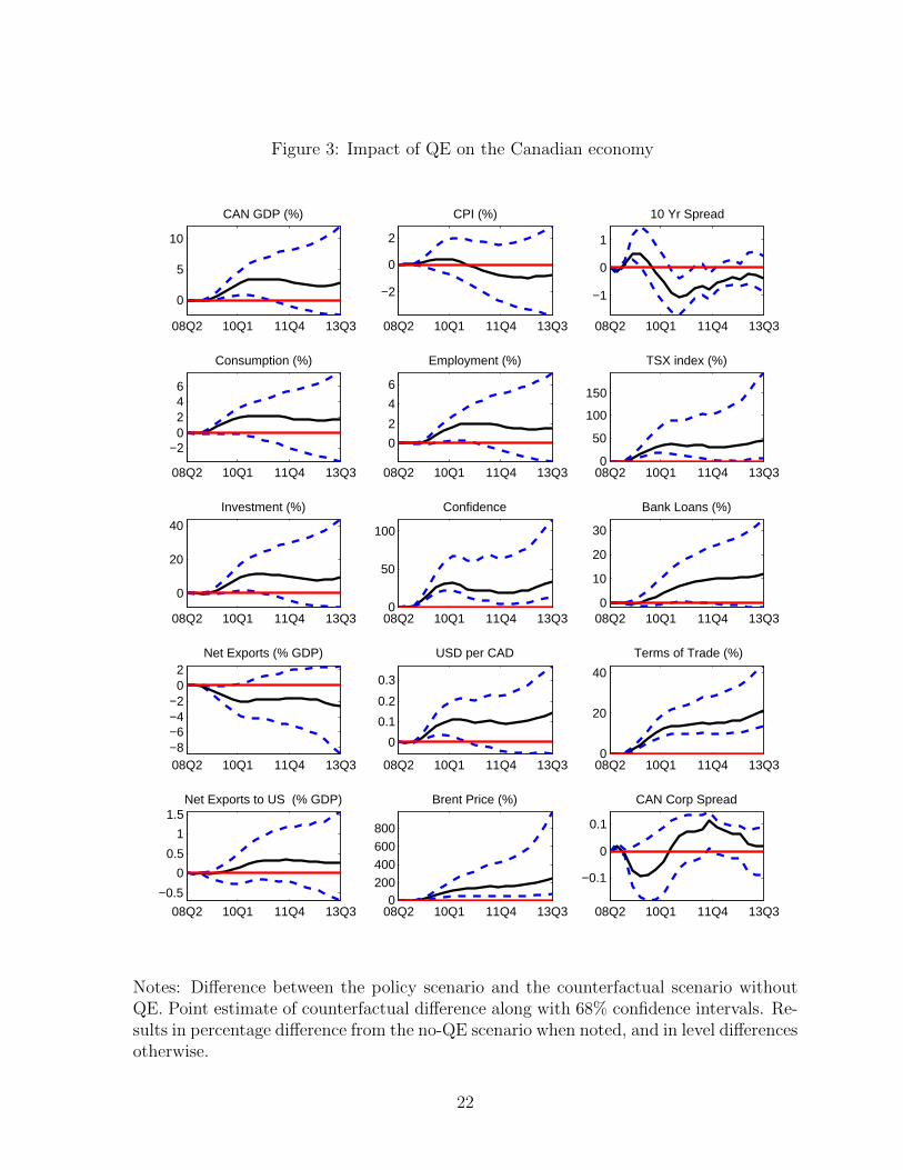
Figure 3: Impact of QE on the Canadian economy

08Q2 10Q1 11Q4 13Q3

0

5

10

CAN GDP (%)

08Q2 10Q1 11Q4 13Q3

−2

0

2

CPI (%)

08Q2 10Q1 11Q4 13Q3

−1

0

1

10 Yr Spread

08Q2 10Q1 11Q4 13Q3

−20246

Consumption (%)

08Q2 10Q1 11Q4 13Q3

0

2

4

6

Employment (%)

08Q2 10Q1 11Q4 13Q30

50

100

150

TSX index (%)

08Q2 10Q1 11Q4 13Q3

0

20

40

Investment (%)

08Q2 10Q1 11Q4 13Q30

50

100

Confidence

08Q2 10Q1 11Q4 13Q30

10

20

30

Bank Loans (%)

08Q2 10Q1 11Q4 13Q3−8−6−4−2

02

Net Exports (% GDP)

08Q2 10Q1 11Q4 13Q3

0

0.1

0.2

0.3

USD per CAD

08Q2 10Q1 11Q4 13Q30

20

40

Terms of Trade (%)

08Q2 10Q1 11Q4 13Q3

−0.5

0

0.5

1

1.5Net Exports to US (% GDP)

08Q2 10Q1 11Q4 13Q30

200400600800

Brent Price (%)

08Q2 10Q1 11Q4 13Q3

−0.1

0

0.1

CAN Corp Spread

Notes: Difference between the policy scenario and the counterfactual scenario withoutQE. Point estimate of counterfactual difference along with 68% confidence intervals. Re-sults in percentage difference from the no-QE scenario when noted, and in level differencesotherwise.

22

Figure 4: Impact of QE on Canadian global trade by product

08Q2 10Q1 11Q4 13Q30

20

40

60

Goo

ds

Exports

08Q2 10Q1 11Q4 13Q30

20

40

60

Imports

08Q2 10Q1 11Q4 13Q3

−6

−4

−2

0

2Net Exports

08Q2 10Q1 11Q4 13Q30

20

40

60

For

estr

y

08Q2 10Q1 11Q4 13Q30

20

40

60

08Q2 10Q1 11Q4 13Q3−0.2

0

0.2

0.4

08Q2 10Q1 11Q4 13Q3

−20

0

20

Ene

rgy

08Q2 10Q1 11Q4 13Q3

0

50

100

150

08Q2 10Q1 11Q4 13Q3−4

−2

0

08Q2 10Q1 11Q4 13Q30

20

40

60

80

Met

al P

rodu

cts

08Q2 10Q1 11Q4 13Q30

20

40

60

08Q2 10Q1 11Q4 13Q3

0

0.5

1

1.5

08Q2 10Q1 11Q4 13Q3

0

20

40

60

Che

mic

al

08Q2 10Q1 11Q4 13Q3

0

20

40

08Q2 10Q1 11Q4 13Q3−0.5

0

0.5

Notes: Difference between the policy scenario and the counterfactual scenario withoutQE. Point estimate of counterfactual difference along with 68% confidence intervals. Re-sults in percentage difference from the no-QE scenario when noted, and in level differencesotherwise.

23

Figure 5: Impact of QE on Canadian global trade by product

08Q2 10Q1 11Q4 13Q3−20

0

20

40

Indu

stria

l M&

E

Exports

08Q2 10Q1 11Q4 13Q3

0

20

40

60

Imports

08Q2 10Q1 11Q4 13Q3−1.5

−1

−0.5

0

0.5Net Exports

08Q2 10Q1 11Q4 13Q30

50

100

Ele

ctric

al

08Q2 10Q1 11Q4 13Q30

50

100

08Q2 10Q1 11Q4 13Q3

−2

−1

0

08Q2 10Q1 11Q4 13Q30

100

200

300

Aut

o

08Q2 10Q1 11Q4 13Q30

100

200

08Q2 10Q1 11Q4 13Q3

−1.5−1

−0.50

0.5

08Q2 10Q1 11Q4 13Q3

−100

102030

Con

s G

oods

08Q2 10Q1 11Q4 13Q3−10

0

10

20

08Q2 10Q1 11Q4 13Q3

−1

0

1

08Q2 10Q1 11Q4 13Q3

−20

−10

0

10

Ser

vice

s

08Q2 10Q1 11Q4 13Q3

0

10

20

30

08Q2 10Q1 11Q4 13Q3

−2

−1

0

Notes: Difference between the policy scenario and the counterfactual scenario withoutQE. Point estimate of counterfactual difference along with 68% confidence intervals. Re-sults in percentage difference from the no-QE scenario when noted, and in level differencesotherwise.

24

Figure 6: Impact of QE on the Canadian GDP by industry

08Q2 10Q1 11Q4 13Q30

10

20

30Goods

08Q2 10Q1 11Q4 13Q3−10

0

10

Mining

08Q2 10Q1 11Q4 13Q30

20

40

Manufactuing

08Q2 10Q1 11Q4 13Q3−4−2

024

Services

08Q2 10Q1 11Q4 13Q3

0

5

10

15

Utility

08Q2 10Q1 11Q4 13Q3

0

10

20

Construction

08Q2 10Q1 11Q4 13Q3

−505

1015

Retail trade

08Q2 10Q1 11Q4 13Q3−30

−20

−10

0

Arts

08Q2 10Q1 11Q4 13Q30

10

20

30

Accommodation

Notes: Difference between the policy scenario and the counterfactual scenario withoutQE. Point estimate of counterfactual difference along with 68% confidence intervals. Re-sults in percentage difference from the no-QE scenario when noted, and in level differencesotherwise.

25

Figure 7: Impact of QE on the U.S. and Canadian economy – alternative case

Panel A: U.S.

08Q2 10Q1 11Q4 13Q3

0

5

10

US GDP (%)

08Q2 10Q1 11Q4 13Q30

2

4

6

PCE price (%)

08Q2 10Q1 11Q4 13Q3−2

−1.5

−1

−0.5

0

0.510 Yr Spread

08Q2 10Q1 11Q4 13Q30

50

100

150

S&P 500 index (%)

08Q2 10Q1 11Q4 13Q3−1

0

1

2

3Net Exports (% GDP)

08Q2 10Q1 11Q4 13Q3

−10

0

10

Exchange Rate (%)

Panel B: Canada

08Q2 10Q1 11Q4 13Q3

0

5

10

CAN GDP (%)

08Q2 10Q1 11Q4 13Q3

0

2

4

6

CPI (%)

08Q2 10Q1 11Q4 13Q3

−2

−1

0

1

2

10 Yr Spread

08Q2 10Q1 11Q4 13Q3

0

50

100

150TSX index (%)

08Q2 10Q1 11Q4 13Q3−10

−8

−6

−4

−2

0Net Exports (% GDP)

08Q2 10Q1 11Q4 13Q30

20

40

60

80

USD per CAD

Notes: Difference between the policy scenario and the counterfactual scenario withoutQE. Point estimate of counterfactual difference along with 68% confidence intervals. Re-sults in percentage difference from the no-QE scenario when noted, and in level differencesotherwise.

26

Figure 8: Impulse responses of a 100 bps reduction in the effective federal funds rate

Panel A: U.S.

5 10 15 200

2

4

6

8

x 10−3 US GDP

5 10 15 20

−3

−2

−1

0

1x 10−3PCE price index

5 10 15 20−1

−0.5

0

Eff Funds Rate

5 10 15 20

−0.04

−0.02

0

0.02S&P 500 index

5 10 15 20

−10

−5

0

x 10−3Net Exports

5 10 15 20

−0.02

−0.01

0

Exchange Rate

Panel B: Canada

5 10 15 200

0.005

0.01

CAN GDP

5 10 15 20

−6

−4

−2

0x 10−3 CPI

5 10 15 20−1

−0.5

0

3m Treasury Yield

5 10 15 200

0.02

0.04

0.06

0.08TSX index

5 10 15 20

−20

−15

−10

−5

0

x 10−3Net Exports

5 10 15 20

0

0.01

0.02

USD per CAD

Notes: Impulse-response functions along with 68% confidence bands. Data span from1983Q1 through 2008Q2.

27

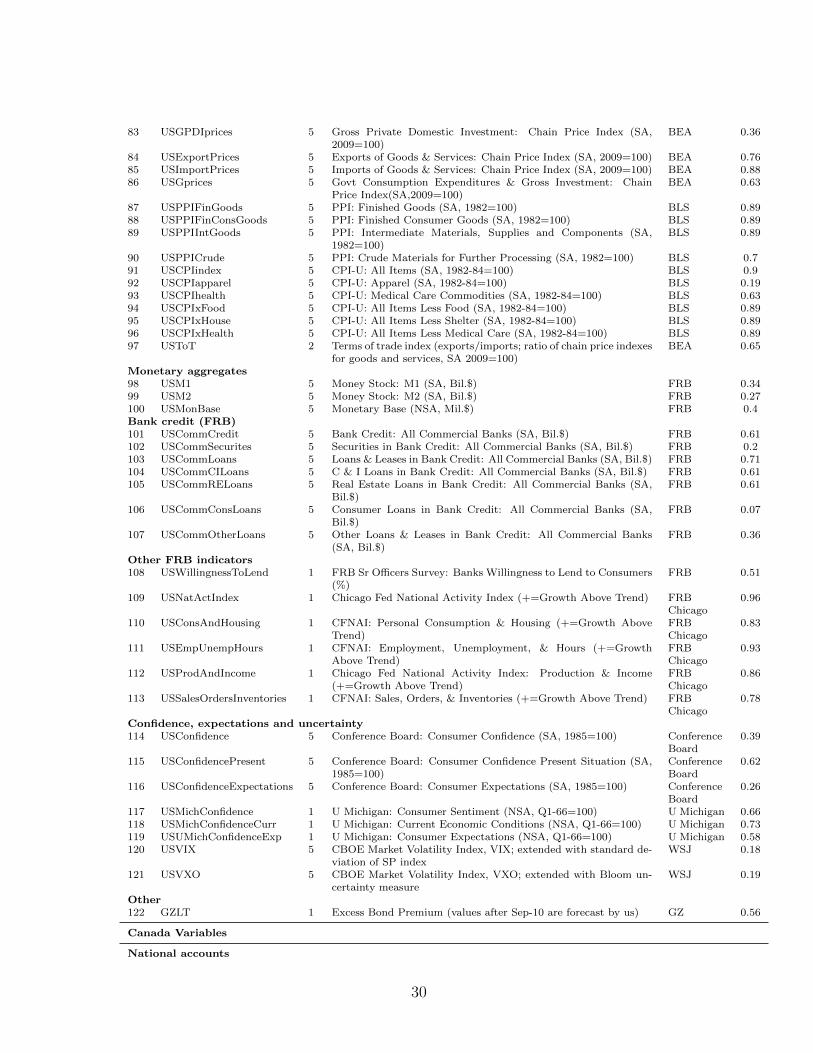
Appendix: Data Description

Format is: series number, series mnemonic, transformation code, series description,source, and the degree to which factors included in the baseline specification explainthe variation of the variable (R-squared). All data available from 1983Q1-2013Q3. Thetransformation codes are: 1 - no transformation; 2 - first difference; 4 - logarithm; 5 -first difference of logarithm. The majority of series were taken from Haver Analytics.

Sources: FRB - Federal Reserve Board, UST - U.S. Treasury, BEA - Bureau ofEconomic Analysis, JPM - JP Morgan, BLS - Bureau of Labor Statistics, ISM -Institute for Supply Management, CB - Census Bureau, S&P - Standard and Poor’s,FRB-C - Federal Reserve Bank of Chicago, GZ - Gilchrist and Zakrajsek 2012, BoC- Bank of Canada, Statcan - Statistics Canada, TSX - Toronto Stock Exchange, IMF- International Monetary Fund, CMHC - Canada Mortgage and Housing Corporation,BIS - Bank for International Settlements

US Variables

Monetary policy1 USEffFedFundsRate 1 Federal Funds [Effective] Rate (% p.a.) FRB 1.002 QE2 2 Fed Res Banks: UST Security Holdings: Over 5 Yrs + Mortgage-

Backed Securities Held Outright (EOP, Mil.$)FRB 1.00

National income and products accounts3 USrGDP 5 Real Gross Domestic Product (SAAR, Bil.Chn.2009$) BEA 0.694 USrC 5 Real Personal Consumption Expenditures (SAAR, Bil.Chn.2009$) BEA 0.535 USrI 5 Real Gross Private Domestic Investment (SAAR, Bil.Chn.2009$) BEA 0.626 USrExports 5 Real Exports of Goods & Services (SAAR, Bil.Chn.2009$) BEA 0.527 USrImports 5 Real Imports of Goods & Services (SAAR, Bil.Chn.2009$) BEA 0.668 USrG 5 Real Government Consumption Expenditures & Gross Invest-

ment(SAAR, Bil.Chn.2009$)BEA 0.34

9 USnExports 5 Exports of Goods and Services (SAAR, Bil.$) BEA 0.6910 USnExportsReceipts 5 Exports: Income Receipts from ROW (SAAR, Bil.$) BEA 0.6111 USnImports 5 Imports of Goods and Services (SAAR, Bil.$) BEA 0.812 USnImportsPayments 5 Imports: Income Payments to ROW (SAAR, Bil.$) BEA 0.4213 USnGDP 5 Gross Domestic Product (SAAR, Bil.$) BEA 0.75Real output and income14 USIPFinalNonind 5 Industrial Production: Final Products and Nonindustrial Supplies

(SA, 2007=100)FRB 0.88

15 USIPFinal 5 Industrial Production: Final Products (SA, 2007=100) FRB 0.8416 USIPCons 5 Industrial Production: Consumer Goods (SA, 2007=100) FRB 0.6217 USIPConsDur 5 Industrial Production: Durable Consumer Goods (SA, 2007=100) FRB 0.6318 USIPConsNonDur 5 Industrial Production: Nondurable Consumer Goods (SA,

2007=100)FRB 0.23

19 USIPBusi 5 Industrial Production: Business Equipment (SA, 2007=100) FRB 0.8120 USIPMat 5 Industrial Production: Materials (SA, 2007=100) FRB 0.8621 USIPMatDur 5 Industrial Production: Durable Goods Materials (SA, 2007=100) FRB 0.8822 USIPMatNonDur 5 Industrial Production: Nondurable Goods Materials (SA,

2007=100)FRB 0.61

23 USIPMan 5 Industrial Production: Manufacturing [NAICS] (SA, 2007=100) FRB 0.9124 USIPMin 5 Industrial Production: Mining (SA, 2007=100) FRB 0.2725 USIPUtl 5 Industrial Production: Electric and Gas Utilities (SA, 2007=100) FRB 0.0626 USIPindex 5 Industrial Production Index (SA, 2007=100) FRB 0.91Employment27 USLabourForce 5 Civilian Labor Force: 16 yr + (SA, Thous) BLS 0.3128 USUnempRate 5 Civilian Unemployment Rate: 16 yr + (SA, %) BLS 0.8329 USUnempLess5w 5 Civilians Unemployed for Less Than 5 Weeks (SA, Thous.) BLS 0.3530 USUnemp5to14w 5 Civilians Unemployed for 5-14 Weeks (SA, Thous.) BLS 0.61

28

31 USUnemp15to26w 5 Civilians Unemployed for 15-26 Weeks (SA, Thous.) BLS 0.5532 USEmpNonfarm 5 All Employees: Total Nonfarm (SA, Thous) BLS 0.8933 USEmpIndustry 5 All Employees: Total Private Industries (SA, Thous) BLS 0.8934 USEmpGoodsIndustry 5 All Employees: Goods-producing Industries (SA, Thous) BLS 0.8935 USEmpLog 5 All Employees: Logging (SA, Thous) BLS 0.3436 USEmpMin 5 All Employees: Mining (SA, Thous) BLS 0.5437 USEmpUtl 5 All Employees: Utilities (SA, Thous) BLS 0.238 USEmpCon 5 All Employees: Construction (SA, Thous) BLS 0.8239 USEmpMan 5 All Employees: Manufacturing (SA, Thous) BLS 0.8540 USEmpManDur 5 All Employees: Durable Goods Manufacturing (SA, Thous) BLS 0.8741 USEmpManNonDur 5 All Employees: Nondurable Goods Manufacturing (SA, Thous) BLS 0.6842 USEmpSvc 5 All Employees: Private Service-providing Industries (SA, Thous) BLS 0.8543 USEmpTrn 5 All Employees: Transportation & Warehousing (SA, Thous) BLS 0.6844 USEmpRet 5 All Employees: Retail Trade (SA, Thous) BLS 0.7445 USEmpWht 5 All Employees: Wholesale Trade (SA, Thous) BLS 0.7746 USEmpFin 5 All Employees: Financial Activities (SA, Thous) BLS 0.5547 USEmpInf 5 All Employees: Information Services (SA, Thous) BLS 0.2548 USEmpGov 5 All Employees: Government (SA, Thous) BLS 0.3349 USEmpIndex 1 ISM Mfg: Employment Index (SA, 50+ = Econ Expand) ISM 0.76Housing starts and sales50 USHousingStarts 4 Housing Starts (SAAR, Thous.Units) CB 0.8451 USHousingStartsNE 4 Housing Starts: Northeast (SAAR, Thous.Units) CB 0.8152 USHousingStartsMidwest 4 Housing Starts: Midwest (SAAR, Thous.Units) CB 0.6953 USHousingStartsSouth 4 Housing Starts: South (SAAR, Thous.Units) CB 0.7754 USHousingStartsWest 4 Housing Starts: West (SAAR, Thous.Units) CB 0.8455 USNewHousingPermits 4 New Pvt Housing Units Authorized by Building Permit (SAAR,

Thous.Units)CB 0.82

ISM (NAPM) manufacturing survey56 USInventories 1 ISM Mfg: Inventories Index (SA, 50+ = Econ Expand) ISM 0.4957 USNewOrders 1 ISM Mfg: New Orders Index (SA, 50+ = Econ Expand) ISM 0.858 USDeliveries 1 ISM Mfg: Supplier Deliveries Index (SA, 50+ = Slower) ISM 0.39Stock prices59 USSP500index 5 S&P 500 Stock Price Index (1941-43=10) WSJ 0.2660 USSP500IndusIndex 5 S&P 500 Industrial Stock Price Index (1941-43=10) S&P 0.24Exchange rates61 USNEER 5 JP Morgan Narrow Nominal Effective Exchange Rate Index: U.S.

(2000=100)JP Morgan 0.27

62 CHFzUSD 5 Foreign Exchange Rate: Switzerland (Swiss Franc/US$) FRB 0.1263 JPYzUSD 5 Foreign Exchange Rate: Japan (Yen/US$) FRB 0.0964 USDzGBP 5 Foreign Exchange Rate: United Kingdom (US$/Pound) FRB 0.21Interest rates65 US3mYield 1 3-Month Treasury Bills, Secondary Market (% p.a.) FRB 0.9966 US6mYield 1 6-Month Treasury Bills, Secondary Market (% p.a.) FRB 0.9967 US1yYield 1 1-Year Treasury Bill Yield at Constant Maturity (%) UST 0.9968 US5yYield 1 5-Year Treasury Note Yield at Constant Maturity (%) UST 0.9669 US10yYield 1 10-Year Treasury Bond Yield at Constant Maturity (%) UST 0.9370 USAAAyield 1 Moody’s Seasoned Aaa Corporate Bond Yield (% p.a.) FRB 0.9171 USBAAyield 1 Moody’s Seasoned Baa Corporate Bond Yield (% p.a.) FRB 0.8972 ShadowRate 1 Shadow rate Wu and

Xia 20130.99

73 US6mSpread 1 US6mYield - US3mYield FRB 0.1674 US1ySpread 1 US1yYield - US3mYield UST, FRB 0.5475 US5ySpread 1 US5yYield - US3mYield UST, FRB 0.6576 US10ySpread 1 US10yYield - US3mYield UST, FRB 0.6577 USCorporateSpread 1 USBAAyield - USAAAyield FRB 0.5Balance of payments78 USCurrAcctBal 2 BOP: Balance on Current Account (SA, Mil.$) BEA 0.3879 USKInflows 2 BOP: For Assets in the U.S., Net: Cap Inflow Ex Fin Derivatives

+ (SA, Mil.$)BEA 0.05

80 USKOutflows 2 BOP: U.S. Assets Abroad, Net: Outflow Excl Financial Deriva-tives (-) (SA, Mil.$)

BEA 0.03

Price indexes81 USGDPprices 5 Gross Domestic Product: Chain Price Index (SA, 2009=100) BEA 0.4882 USPCEprices 5 Personal Consumption Expenditures: Chain Price Index (SA,

2009=100)BEA 0.88

29

83 USGPDIprices 5 Gross Private Domestic Investment: Chain Price Index (SA,2009=100)

BEA 0.36

84 USExportPrices 5 Exports of Goods & Services: Chain Price Index (SA, 2009=100) BEA 0.7685 USImportPrices 5 Imports of Goods & Services: Chain Price Index (SA, 2009=100) BEA 0.8886 USGprices 5 Govt Consumption Expenditures & Gross Investment: Chain

Price Index(SA,2009=100)BEA 0.63

87 USPPIFinGoods 5 PPI: Finished Goods (SA, 1982=100) BLS 0.8988 USPPIFinConsGoods 5 PPI: Finished Consumer Goods (SA, 1982=100) BLS 0.8989 USPPIIntGoods 5 PPI: Intermediate Materials, Supplies and Components (SA,

1982=100)BLS 0.89

90 USPPICrude 5 PPI: Crude Materials for Further Processing (SA, 1982=100) BLS 0.791 USCPIindex 5 CPI-U: All Items (SA, 1982-84=100) BLS 0.992 USCPIapparel 5 CPI-U: Apparel (SA, 1982-84=100) BLS 0.1993 USCPIhealth 5 CPI-U: Medical Care Commodities (SA, 1982-84=100) BLS 0.6394 USCPIxFood 5 CPI-U: All Items Less Food (SA, 1982-84=100) BLS 0.8995 USCPIxHouse 5 CPI-U: All Items Less Shelter (SA, 1982-84=100) BLS 0.8996 USCPIxHealth 5 CPI-U: All Items Less Medical Care (SA, 1982-84=100) BLS 0.8997 USToT 2 Terms of trade index (exports/imports; ratio of chain price indexes

for goods and services, SA 2009=100)BEA 0.65

Monetary aggregates98 USM1 5 Money Stock: M1 (SA, Bil.$) FRB 0.3499 USM2 5 Money Stock: M2 (SA, Bil.$) FRB 0.27100 USMonBase 5 Monetary Base (NSA, Mil.$) FRB 0.4Bank credit (FRB)101 USCommCredit 5 Bank Credit: All Commercial Banks (SA, Bil.$) FRB 0.61102 USCommSecurites 5 Securities in Bank Credit: All Commercial Banks (SA, Bil.$) FRB 0.2103 USCommLoans 5 Loans & Leases in Bank Credit: All Commercial Banks (SA, Bil.$) FRB 0.71104 USCommCILoans 5 C & I Loans in Bank Credit: All Commercial Banks (SA, Bil.$) FRB 0.61105 USCommRELoans 5 Real Estate Loans in Bank Credit: All Commercial Banks (SA,

Bil.$)FRB 0.61

106 USCommConsLoans 5 Consumer Loans in Bank Credit: All Commercial Banks (SA,Bil.$)

FRB 0.07

107 USCommOtherLoans 5 Other Loans & Leases in Bank Credit: All Commercial Banks(SA, Bil.$)

FRB 0.36

Other FRB indicators108 USWillingnessToLend 1 FRB Sr Officers Survey: Banks Willingness to Lend to Consumers

(%)FRB 0.51

109 USNatActIndex 1 Chicago Fed National Activity Index (+=Growth Above Trend) FRBChicago

0.96

110 USConsAndHousing 1 CFNAI: Personal Consumption & Housing (+=Growth AboveTrend)

FRBChicago

0.83

111 USEmpUnempHours 1 CFNAI: Employment, Unemployment, & Hours (+=GrowthAbove Trend)

FRBChicago

0.93

112 USProdAndIncome 1 Chicago Fed National Activity Index: Production & Income(+=Growth Above Trend)

FRBChicago

0.86

113 USSalesOrdersInventories 1 CFNAI: Sales, Orders, & Inventories (+=Growth Above Trend) FRBChicago

0.78

Confidence, expectations and uncertainty114 USConfidence 5 Conference Board: Consumer Confidence (SA, 1985=100) Conference

Board0.39

115 USConfidencePresent 5 Conference Board: Consumer Confidence Present Situation (SA,1985=100)

ConferenceBoard

0.62

116 USConfidenceExpectations 5 Conference Board: Consumer Expectations (SA, 1985=100) ConferenceBoard

0.26

117 USMichConfidence 1 U Michigan: Consumer Sentiment (NSA, Q1-66=100) U Michigan 0.66118 USMichConfidenceCurr 1 U Michigan: Current Economic Conditions (NSA, Q1-66=100) U Michigan 0.73119 USUMichConfidenceExp 1 U Michigan: Consumer Expectations (NSA, Q1-66=100) U Michigan 0.58120 USVIX 5 CBOE Market Volatility Index, VIX; extended with standard de-

viation of SP indexWSJ 0.18

121 USVXO 5 CBOE Market Volatility Index, VXO; extended with Bloom un-certainty measure

WSJ 0.19

Other122 GZLT 1 Excess Bond Premium (values after Sep-10 are forecast by us) GZ 0.56

Canada Variables

National accounts

30

123 CANrGDP 5 Canada: Gross Domestic Product at Market Prices (SAAR,Mil.Chn.2007.C$)

Statcan 0.76

124 CANrExports 5 Canada: GDP: Exports of Goods and Services: Total (SAAR,Mil.Chn.2007.C$)

Statcan 0.67

125 CANrImports 5 Canada: GDP: Imports of Goods and Services: Total (SAAR,Mil.Chn.2007.C$)

Statcan 0.65

126 CANrC 5 Canada:GDP: Household Final Consumption Exp: Total (SAAR,Mil.Chn.2007.C$)

Statcan 0.44

127 CANrI 5 Canada: GDP: Business Gross Fixed Capital Formation (SAAR,Mil.Chn.2007.C$)

Statcan 0.57

128 CANrGC 5 Canada:GDP: General Govt Final Consumption Expenditure(SAAR,Mil.Chn.2007.C$)

Statcan 0.22

129 CANrGI 5 Canada: GDP: Gross Fixed Capital Form: General Govern-ment(SAAR, Mil.Chn.2007.C$)

Statcan 0.28

GDP by NAICS130 CANryGoods 5 Canada: GDP: Goods-Producing Industries (SAAR, Mil.2007.C$) Statcan 0.77131 CANryAgr 5 Canada: GDP: Agriculture, Forestry, Fishing and Hunting

(SAAR, Mil.2007.C$)Statcan 0.1

132 CANryMin 5 Canada: GDP: Mining, Quarrying, and Oil and Gas Extraction(SAAR, Mil.2007.C$)

Statcan 0.27

133 CANryUtl 5 Canada: GDP: Utilities (SAAR, Mil.2007.C$) Statcan 0.11134 CANryCon 5 Canada: GDP: Construction (SAAR, Mil.2007.C$) Statcan 0.41135 CANryMan 5 Canada: GDP: Manufacturing (SAAR, Mil.2007.C$) Statcan 0.79136 CANrySvc 5 Canada: GDP: Service-Producing Industries (SAAR,

Mil.2007.C$)Statcan 0.54

137 CCANryWht 5 Canada: GDP: Wholesale Trade (SAAR, Mil.2007.C$) Statcan138 CANryRet 5 Canada: GDP: Retail Trade (SAAR, Mil.2007.C$) Statcan 0.16139 CANryTrn 5 Canada: GDP: Transportation and Warehousing (SAAR,

Mil.2007.C$)Statcan 0.48

140 CANryInf 5 Canada: GDP: Information and Cultural Industries (SAAR,Mil.2007.C$)

Statcan 0.32

141 CANryPro 5 Canada: GDP: Professional, Scientific and Technical Ser-vices(SAAR, Mil.2007.C$)

Statcan 0.31

142 CANryAdm 5 Can:GDP:Admin\Support, Waste Management & RemediationService(SAAR,Mil.2007.C$)

Statcan 0.16

143 CANryEdu 5 Canada: GDP: Educational Services (SAAR, Mil.2007.C$) Statcan 0.1144 CANryHlt 5 Canada: GDP: Health Care and Social Assistance (SAAR,

Mil.2007.C$)Statcan 0.18

145 CANryArt 5 Canada: GDP: Arts, Entertainment and Recreation (SAAR,Mil.2007.C$)

Statcan 0.1

146 CANryAcc 5 Canada: GDP: Accommodation and Food Services (SAAR,Mil.2007.C$)

Statcan 0.19

147 CANryOth 5 Canada: GDP: Other Services (Except Public Administration)(SAAR, Mil.2007.C$)

Statcan 0.28

148 CANryPub 5 Canada: GDP: Public Administration (SAAR, Mil.2007.C$) Statcan 0.25Trade flows by NAPCS149 CANrGoodsExports 5 Canada: Total Exports of Goods (SAAR, Mil.Chn.2007.C$) Statcan 0.64150 CANrAgrExports 5 Canada: Exports of Farm, Fishing & Intermed Food Prod-

ucts(SAAR, Mil.Chn.2007.C$)Statcan 0.07

151 CANrEnergyExports 5 Canada: Exports of Energy Products (SAAR, Mil.Chn.2007.C$) Statcan 0.09152 CANrOreExports 5 Canada: Exports of Metal Ores and Nonmetallic Minerals (SAAR,

Mil.Chn.2007.C$)Statcan 0.17

153 CANrMetalExports 5 Canada: Exports of Metal and Nonmetallic Mineral Prod-ucts(SAAR, Mil.Chn.2007.C$)

Statcan 0.17

154 CANrChemExports 5 Canada: Exp of Basic & Ind Chem, Plastics & RubberProds(SAAR, Mil.Chn.2007.C$)

Statcan 0.28

155 CANrForExports 5 Canada: Exports of Forestry Prods & Bldg & PackagingMtls(SAAR, Mil.Chn.2007.C$)

Statcan 0.32

156 CANrIndExports 5 Canada: Exports of Industrial Machinery, Equip & Parts (SAAR,Mil.Chn.2007.C$)

Statcan 0.47

157 CANrElecExports 5 Canada: Exports of Electronic & Electrical Equip & Parts(SAAR, Mil.Chn.2007.C$)

Statcan 0.42

158 CANrAutoExports 5 Canada: Exports of Motor Vehicles and Parts (SAAR,Mil.Chn.2007.C$)

Statcan 0.46

159 CANrTranspExports 5 Canada: Exports of Aircraft & Other Transp Eqpt & Parts(SAAR, Mil.Chn.2007.C$)

Statcan 0.19

31

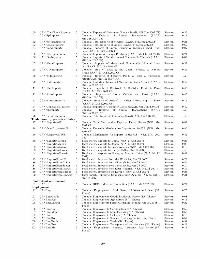
160 CANrConsGoodsExports 5 Canada: Exports of Consumer Goods (SAAR, Mil.Chn.2007.C$) Statcan 0.35161 CANrSpExports 5 Canada: Exports of Special Transactions (SAAR,

Mil.Chn.2007.C$)Statcan 0.14

162 CANrServiceExports 5 Canada: Total Exports of Services (SAAR, Mil.Chn.2007.C$) Statcan 0.21163 CANrGoodsImports 5 Canada: Total Imports of Goods (SAAR, Mil.Chn.2007.C$) Statcan 0.62164 CANrFoodImports 5 Canada: Imports of Farm, Fishing & Intermed Food Prod-

ucts(SAAR, Mil.Chn.2007.C$)Statcan 0.02

165 CANrEnergyImports 5 Canada: Imports of Energy Products (SAAR, Mil.Chn.2007.C$) Statcan 0.21166 CANrOreImports 5 Canada: Imports of Metal Ores and Nonmetallic Minerals (SAAR,

Mil.Chn.2007.C$)Statcan 0.09

167 CANrMetalImports 5 Canada: Imports of Metal and Nonmetallic Mineral Prod-ucts(SAAR, Mil.Chn.2007.C$)

Statcan 0.37

168 CANrChemImports 5 Canada: Imp of Basic & Ind Chem, Plastics & RubberProds(SAAR, Mil.Chn.2007.C$)

Statcan 0.27

169 CANrBldgImports 5 Canada: Imports of Forestry Prods & Bldg & PackagingMtls(SAAR, Mil.Chn.2007.C$)

Statcan 0.2

170 CANrIndImports 5 Canada: Imports of Industrial Machinery, Equip & Parts (SAAR,Mil.Chn.2007.C$)

Statcan 0.42

171 CANrElecImports 5 Canada: Imports of Electronic & Electrical Equip & Parts(SAAR, Mil.Chn.2007.C$)

Statcan 0.43

172 CANrAutoImports 5 Canada: Imports of Motor Vehicles and Parts (SAAR,Mil.Chn.2007.C$)

Statcan 0.45

173 CANrTranspImports 5 Canada: Imports of Aircraft & Other Transp Eqpt & Parts(SAAR, Mil.Chn.2007.C$)

Statcan 0.11

174 CANrConsGoodsImports 5 Canada: Imports of Consumer Goods (SAAR, Mil.Chn.2007.C$) Statcan 0.42175 CANrSpImports 5 Canada: Imports of Special Transactions (SAAR,

Mil.Chn.2007.C$)Statcan 0.1

176 CANrServiceImports 5 Canada: Total Imports of Services (SAAR, Mil.Chn.2007.C$) Statcan 0.4Trade flows by partner country177 CANrExportstoUS 5 Canada: Total Merchandise Exports: United States (NSA, Mn.

2007 C$)Statcan 0.87

178 CANrDomExportstoUS 5 Canada: Domestic Merchandise Exports to the U.S. (NSA, Mn.2007 C$)

Statcan 0.85

179 CANrReexportsToUS 5 Canada: Merchandise Re-Exports to the U.S. (NSA, Mn. 2007C$)

Statcan 0.42

180 CANrExportstoChina 5 Total merch. exports to China (NSA, Mn.C$ 2007) Statcan 0.27181 CANrExportstoJapan 5 Total merch. exports to Japan (NSA, Mn.C$ 2007) Statcan 0.26182 CANrExportstoLatAm 5 Total merch. exports to Latin America (NSA, Mn.C$ 2007) Statcan 0.15183 CANrExportstoEurope 5 Total merch. exports to Europe (NSA, Mn.C$ 2007) Statcan 0.4184 CANrExportstoEmAsia 5 Total merch. exports to Emerging Asia ex. China (NSA, Mn.C$

2007)Statcan 0.41

185 CANrImportsFromUS 5 Total merch. imports from the US (NSA, Mn.C$ 2007) Statcan 0.73186 CANrImportsFromChina 5 Total merch. imports from China (NSA, Mn.C$ 2007) Statcan 0.59187 CANrImportsFromJapan 5 Total merch. imports from Japan (NSA, Mn.C$ 2007) Statcan 0.19188 CANrImportsFromLatAm 5 Total merch. imports from Latin America (NSA, Mn.C$ 2007) Statcan 0.36189 CANrImportsFromEurope 5 Total merch. imports from Europe (NSA, Mn.C$ 2007) Statcan 0.28190 CANrImportsFromEmAsia 5 Total merch. imports from Emerging Asia ex. China (NSA,

Mn.C$ 2007)Statcan 0.34

Real output and income191 CANIP 5 Canada: GDP: Industrial Production (SAAR, Mil.2007.C$) Statcan 0.77Employment192 CANEmp 5 Canada: Employment: Both Sexes, 15 Years and Over (SA,

Thous)Statcan 0.75

193 CANEmpGoods 5 Canada: Employment: Goods Producing Sector (SA, Thous) Statcan 0.68194 CANEmpAgr 5 Canada: Employment: Agriculture (SA, Thous) Statcan 0.14195 CANEmpMinFor 5 Canada: Employment: Forestry, Fishing, Mining, Oil & Gas (SA,

Thous)Statcan 0.22

196 CANEmpCon 5 Canada: Employment: Construction (SA, Thous) Statcan 0.52197 CANEmpMan 5 Canada: Employment: Manufacturing (SA, Thous) Statcan 0.55198 CANEmpUtl 5 Canada: Employment: Utilities (SA, Thous) Statcan 0.16199 CANEmpSvc 5 Canada: Employment: Service Producing Sector (SA, Thous) Statcan 0.52200 CANEmpTrade 5 Canada: Employment: Trade (SA, Thous) Statcan 0.31201 CANEmpTrn 5 Canada: Employment: Transport and Warehousing (SA, Thous) Statcan 0.23202 CANEmpFin 5 Canada: Employment: Finance, Insurance, Real Estate (SA,

Thous)Statcan 0.12

32

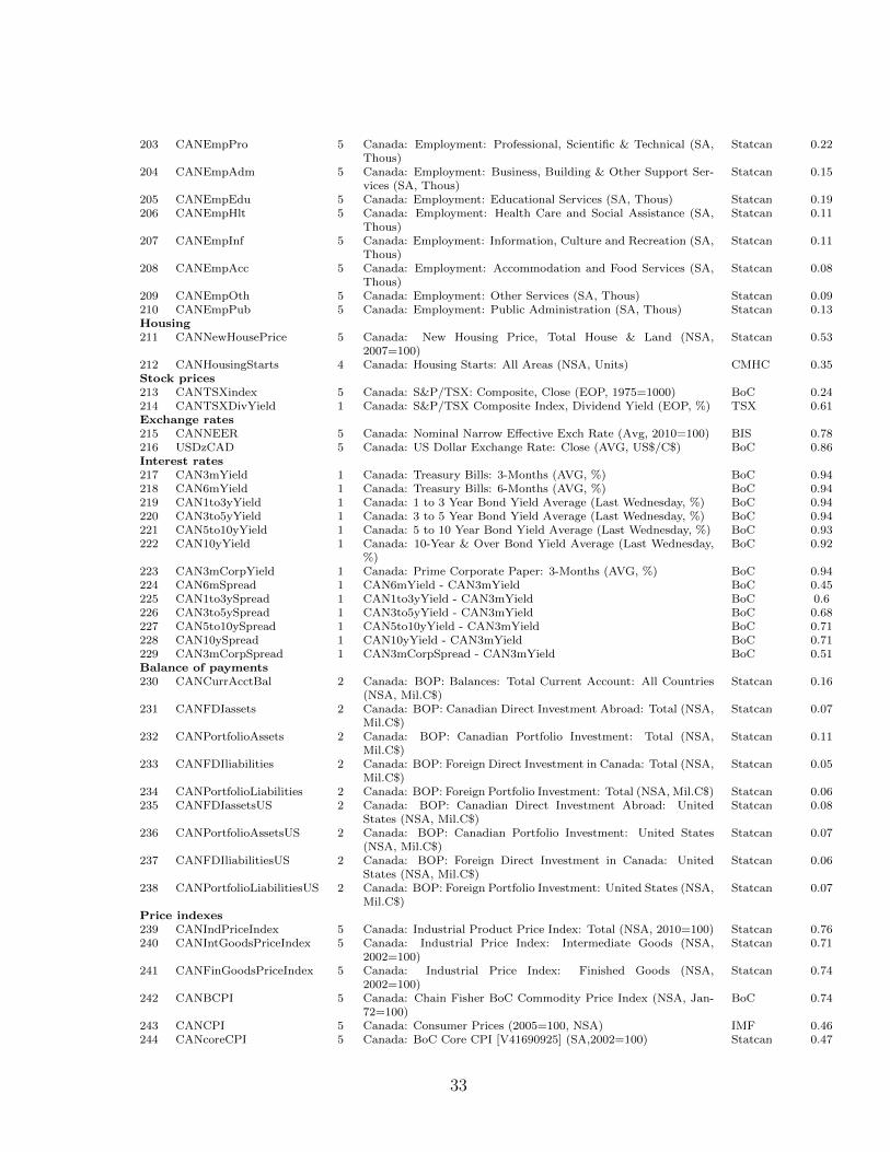
203 CANEmpPro 5 Canada: Employment: Professional, Scientific & Technical (SA,Thous)

Statcan 0.22

204 CANEmpAdm 5 Canada: Employment: Business, Building & Other Support Ser-vices (SA, Thous)

Statcan 0.15

205 CANEmpEdu 5 Canada: Employment: Educational Services (SA, Thous) Statcan 0.19206 CANEmpHlt 5 Canada: Employment: Health Care and Social Assistance (SA,

Thous)Statcan 0.11

207 CANEmpInf 5 Canada: Employment: Information, Culture and Recreation (SA,Thous)

Statcan 0.11

208 CANEmpAcc 5 Canada: Employment: Accommodation and Food Services (SA,Thous)

Statcan 0.08

209 CANEmpOth 5 Canada: Employment: Other Services (SA, Thous) Statcan 0.09210 CANEmpPub 5 Canada: Employment: Public Administration (SA, Thous) Statcan 0.13Housing211 CANNewHousePrice 5 Canada: New Housing Price, Total House & Land (NSA,

2007=100)Statcan 0.53

212 CANHousingStarts 4 Canada: Housing Starts: All Areas (NSA, Units) CMHC 0.35Stock prices213 CANTSXindex 5 Canada: S&P/TSX: Composite, Close (EOP, 1975=1000) BoC 0.24214 CANTSXDivYield 1 Canada: S&P/TSX Composite Index, Dividend Yield (EOP, %) TSX 0.61Exchange rates215 CANNEER 5 Canada: Nominal Narrow Effective Exch Rate (Avg, 2010=100) BIS 0.78216 USDzCAD 5 Canada: US Dollar Exchange Rate: Close (AVG, US$/C$) BoC 0.86Interest rates217 CAN3mYield 1 Canada: Treasury Bills: 3-Months (AVG, %) BoC 0.94218 CAN6mYield 1 Canada: Treasury Bills: 6-Months (AVG, %) BoC 0.94219 CAN1to3yYield 1 Canada: 1 to 3 Year Bond Yield Average (Last Wednesday, %) BoC 0.94220 CAN3to5yYield 1 Canada: 3 to 5 Year Bond Yield Average (Last Wednesday, %) BoC 0.94221 CAN5to10yYield 1 Canada: 5 to 10 Year Bond Yield Average (Last Wednesday, %) BoC 0.93222 CAN10yYield 1 Canada: 10-Year & Over Bond Yield Average (Last Wednesday,

%)BoC 0.92

223 CAN3mCorpYield 1 Canada: Prime Corporate Paper: 3-Months (AVG, %) BoC 0.94224 CAN6mSpread 1 CAN6mYield - CAN3mYield BoC 0.45225 CAN1to3ySpread 1 CAN1to3yYield - CAN3mYield BoC 0.6226 CAN3to5ySpread 1 CAN3to5yYield - CAN3mYield BoC 0.68227 CAN5to10ySpread 1 CAN5to10yYield - CAN3mYield BoC 0.71228 CAN10ySpread 1 CAN10yYield - CAN3mYield BoC 0.71229 CAN3mCorpSpread 1 CAN3mCorpSpread - CAN3mYield BoC 0.51Balance of payments230 CANCurrAcctBal 2 Canada: BOP: Balances: Total Current Account: All Countries

(NSA, Mil.C$)Statcan 0.16

231 CANFDIassets 2 Canada: BOP: Canadian Direct Investment Abroad: Total (NSA,Mil.C$)

Statcan 0.07

232 CANPortfolioAssets 2 Canada: BOP: Canadian Portfolio Investment: Total (NSA,Mil.C$)

Statcan 0.11

233 CANFDIliabilities 2 Canada: BOP: Foreign Direct Investment in Canada: Total (NSA,Mil.C$)

Statcan 0.05

234 CANPortfolioLiabilities 2 Canada: BOP: Foreign Portfolio Investment: Total (NSA, Mil.C$) Statcan 0.06235 CANFDIassetsUS 2 Canada: BOP: Canadian Direct Investment Abroad: United

States (NSA, Mil.C$)Statcan 0.08

236 CANPortfolioAssetsUS 2 Canada: BOP: Canadian Portfolio Investment: United States(NSA, Mil.C$)

Statcan 0.07

237 CANFDIliabilitiesUS 2 Canada: BOP: Foreign Direct Investment in Canada: UnitedStates (NSA, Mil.C$)

Statcan 0.06

238 CANPortfolioLiabilitiesUS 2 Canada: BOP: Foreign Portfolio Investment: United States (NSA,Mil.C$)

Statcan 0.07

Price indexes239 CANIndPriceIndex 5 Canada: Industrial Product Price Index: Total (NSA, 2010=100) Statcan 0.76240 CANIntGoodsPriceIndex 5 Canada: Industrial Price Index: Intermediate Goods (NSA,

2002=100)Statcan 0.71

241 CANFinGoodsPriceIndex 5 Canada: Industrial Price Index: Finished Goods (NSA,2002=100)

Statcan 0.74

242 CANBCPI 5 Canada: Chain Fisher BoC Commodity Price Index (NSA, Jan-72=100)

BoC 0.74

243 CANCPI 5 Canada: Consumer Prices (2005=100, NSA) IMF 0.46244 CANcoreCPI 5 Canada: BoC Core CPI [V41690925] (SA,2002=100) Statcan 0.47

33

245 CANExportPrices 5 Canada: Implicit Price Index: Exports of Goods and Svcs(SA,2007=100)

Statcan 0.8

246 CANExportPricesGoods 5 Canada: Implicit Price Index: Exports of Goods (SA, 2007=100) Statcan 0.79247 CANExportPricesServices 5 Canada: Implicit Price Index: Exports of Services (SA,

2007=100)Statcan 0.46

248 CANToT 5 Canada: Terms of Trade Index (SA, 2007=100) Statcan 0.67Monetary aggregates249 CANM1Plus 5 Canada: M1+ (SA, Mil.C$) BoC 0.23250 CANM2Gross 5 Canada: M2 Gross [V41552796] (SA, Avg, Mil.C$) BoC 0.53251 CANM3Gross 5 Canada: M3 Gross [V41552794] (SA, Avg, Mil.C$) BoC 0.63252 CANMonBase 5 Canada: Monetary Base (SA, Mil.C$) BoC 0.16253 CANMonBaseExRR 5 Canada: Monetary Base Excluding Required Reserves (SA,

Mil.C$)BoC 0.12

Chartered banks254 CANBankAssets 5 Canada: Chartered Banks: Major Assets (Avg, SA, Mil.C$) BoC 0.35255 CANBankLiquidAssets 5 Canada: Chartered Banks: Canadian Dollar Assets, Liquid Assets

(Avg, SA, Mil.C$)BoC 0.22

256 CANBankLessLiquidAssets 5 Canada: Canadian Dollar Assets, Less Liquid Assets (Mil.C$) BoC 0.47257 CANBankResidMtgLoans 5 Canada: Chartered Bank Assets: Residential Mortgage Loans

(SA, Mil.C$)BoC 0.35

258 CANBankLoans 5 Canada: Chartered Bank Assets: Bank Loans (SA, Mil.C$) BoC 0.43259 CANBankGeneralLoans 5 Canada: Genl Loans incl Grain Dealers/Installment Finance

Companies (Mil.C$)BoC 0.42

260 CANBankBusinessLoans 5 Canada: Chartered Bank Assets: Business Loans (SA, Avg Weds,Mil.C$)

BoC 0.36

261 CANBankPersonalLoans 5 Canada: Chartered Bank Assets: Total Personal Loans (SA, AvgWeds, Mil.C$)

BoC 0.36

Private credit262 CANPrivateCredit 5 Canada: Business and Household Credit (SA, Mil.C$) BoC 0.71263 CANHHCredit 5 Canada: Household Credit (SA, Mil.C$) BoC 0.71264 CANConsCredit 5 Canada: Consumer Credit at Month-End (EOP, SA, Mil.C$) BoC 0.51265 CANMtgCredit 5 Canada: Residential Mortgage Credit at Month-End (EOP, SA,

Mil.C$)BoC 0.63

266 CANBusCredit 5 Canada: Business Credit (SA, Mil.C$) BoC 0.57267 CANBusCreditST 5 Canada: Short-Term Business Credit (SA, Mil.C$) BoC 0.65268 CANBusCreditLT 5 Canada: Long-Term Business Credit (SA, Mil.C$) BoC 0.34Confidence and uncertainty269 CANConfidence 5 Conference Board Consumer Confidence Index BoC 0.34270 CANVIX 5 standard deviation of TSX index BoC 0.08Oil prices271 Brent 5 Brent (backcast with WTI), dollar/barrel BoC 0.58

34