international parities and exchange rate determination · international parities and exchange rate...
TRANSCRIPT

MPRAMunich Personal RePEc Archive
International Parities and Exchange RateDetermination
Yan Zhao
31. March 2005
Online at https://mpra.ub.uni-muenchen.de/36967/MPRA Paper No. 36967, posted 27. February 2012 09:53 UTC

International Parities
and Exchange Rate Determination
Yan Zhao*
Abstract
The model of equilibrium exchange rate combining purchasing power parity (PPP)
and uncovered interest parity (UIP) is widely tested using the cointegration approach.
Most of the recent studies, however, are deficient in the treatment of expectations and
the power of tests.
This paper aims at resolving the two deficiencies by deriving and testing the
yen/dollar exchange rate model. Perfect foresight is assumed to circumvent the
expectation problem and a modification of cointegration variables is introduced to
improve the power of tests.
With this new methodology, supportive evidence for the hypothesis of combining
PPP and UIP is found in the short run: cointegration between the future exchange rate,
price and interest rate differentials exists; the error correction model (ECM) is
significant. The paper also suggests that it is the interest rate differential, rather
than the price differential, that explains more of the movement of the nominal
exchange rate in the short run. In the long run, however, the cointegration does not
exist because the interest rate differential becomes exogenous.
* Graduate student in the Master course at the Otaru University of Commerce, Japan. E-mail: [email protected].

Acknowledgements
This paper is written under the supervision of Professor Hiroshi
Shibuya at the Otaru University of Commerce. I still remember the days
when he held two seminars per week for me last year: International
Finance and Time-Series Econometrics, without which I could not have
begun this research. I think he is a great instructor in keeping the balance
between intriguing the student’s interest and teaching hard materials. His
instruction is highly appreciated.
Moreover, Professor Shibuya made many important suggestions and
remarks on this paper. It was my first time to write a research paper and
during the writing process, what he gave me was hints rather than
instructions. He never told me what I should do or should not do. Instead,
he gave me full latitude to try my own idea. I realize now that working out
one’s own idea is really important to do research. It is the combination of
his supervision and my own work that produced this paper.
Special thanks should also be given to Professor Ryosuke Wada, who
taught me Finance and offered DataStream support for this paper. Since
this paper is also the result of my graduate studies, I would like to thank
the following professors: Akihiko Kawaura, Kenji Yamamoto, Shigeru
Nishiyama and Tomoichi Shinotsuka.

Contents
1. Introduction.................................................................................................................. 1
1.1. PPP as the First Exchange Rate Model ............................................................................ 1
1.2. Combining PPP with UIP (CHEER) ................................................................................ 2
1.3. Two Problems of the CHEER Approach.......................................................................... 3
1.4. Solution of the Two Problems.......................................................................................... 5
2. Literature Survey......................................................................................................... 7
2.1 Review of PPP ................................................................................................................. 7
2.1.1. What’s PPP?......................................................................................................... 7
2.1.2. Empirical tests of PPP.......................................................................................... 8
2.2 Review of UIP................................................................................................................ 12
2.2.1. What’s UIP? ....................................................................................................... 12
2.2.2. Empirical test of UIP.......................................................................................... 13
2.3 Cointegration Analysis of PPP and UIP......................................................................... 15
3. Short-Run Analysis (Jan. 1973~Jun. 2004) .............................................................. 18
3.1. Pretests of PPP and UIP ................................................................................................. 18
3.1.1. Unit root process and Dickey-Fuller test............................................................ 18
3.1.2. Nonstationary process and PPP test ................................................................... 19
3.1.3. Stationary process and UIP test.......................................................................... 24
3.2. The Model of Exchange Rate Determination................................................................. 26
3.2.1. Is the relative price enough to determine the exchange rate?............................. 26
3.2.2. The model of exchange rate determination ........................................................ 28
3.3. Econometric Analysis .................................................................................................... 29
3.3.1. Cointegration analysis........................................................................................ 29
3.3.2. The effect of the modification and the increased test power.............................. 31
3.3.3. The error correction model (ECM) .................................................................... 33
3.3.4. Causality test and innovation accounting........................................................... 34
i

4. Long-Run Analysis (Year 1870~2003) ....................................................................... 41
4.1. The CHEER Model of Exchange Rate Determination................................................... 41
4.1.1. Unit root tests ..................................................................................................... 41
4.1.2. The nominal exchange rate determination model .............................................. 45
4.2. Engle-Granger Cointegration Test and ECM ................................................................. 46
4.3. Granger Causality and Johansen Methodology.............................................................. 48
5. Conclusion .................................................................................................................. 53
Appendix............................................................................................................................ 56
Appendix 1: Program Description ............................................................................................. 56
Appendix 2: Data Source and Description................................................................................. 57
Appendix 3: Data Summary....................................................................................................... 58
Appendix 4: Short-Run Forecast Error ...................................................................................... 59
Appendix 5: Long-Run Forecast Error Decomposition ............................................................. 61
References.......................................................................................................................... 62
ii

1. Introduction
Recently the question of exchange rate determination has been extensively
researched. Knowing the level of equilibrium exchange rate is becoming an
important issue in the field of international finance and macroeconomics,
especially with the more integrated world economy. It is of vital importance not
only for individuals and firms engaging in international trade and finance, but
also for the monetary authorities conducting monetary policy. Moreover, the
equilibrium exchange rate is an important macroeconomic policy variable for both
developing and developed countries. As a result, almost all open macroeconomic
theories involve the measurement of equilibrium exchange rate.
1.1.
PPP as the First Exchange Rate Model
In the economic literature, purchasing power parity (PPP), which was put
forth by Cassel (1921)1, is the first theory to measure the equilibrium exchange
rate level. Based on the law of one price (LOP), purchasing power parity states
that the relative price determines the exchange rate movement.
According to the PPP hypothesis, the relative price is the main determinant of
the exchange rate and if written in log forms, the exchange rate should be equal
to the price differential. The common deviation of the exchange rate from the
relative price and the more volatile exchange rate fluctuation in the post-floating
period, however, prompted many economists to test the validity of purchasing
1 Gustav Cassel 1921. The World’s Monetary Problems. London: Constable.
1

power parity 2 . Recent tests of PPP have been typically based on the
investigation of the time series property of the real exchange rate, which can be
seen as the residuals from PPP. These test results3 indicate that PPP may not
hold: the real exchange rates are not always stationary. The failure of PPP in
the short run is common. Even in the long run, the validity of PPP is mixed.
1.2.
Combining PPP with UIP (CHEER)
The failure of PPP caused many people to raise doubt on the PPP as the model
of equilibrium exchange rate. With the great expansion of world financial
markets in the past twenty years, some economists put forward a model of
equilibrium exchange rate that combines the purchasing power parity and
uncovered interest parity (UIP). UIP is derived on the assumption of foreign
exchange market efficiency, i.e., there is no “excessive arbitrage opportunity”.
UIP states the relationship between the exchange rate and the interest rate
differential, indicating that an increasing domestic to foreign interest rate
differential will generate expected depreciation of the exchange rate.
The proponents of the model that combines PPP and UIP argue that PPP
represents the equilibrium of goods market only. They suggest that the price
levels are not sufficient to capture all the factors causing fluctuations of the
exchange rate without taking the world financial markets into account.
According to their arguments, the exchange rate deviation from PPP is not
2 Engel and Morley (2001) proposed a different view and they developed a model to show that the nominal exchange rate converges much more slowly than the prices. 3 See Chapter 2 of this paper for more details of the literature survey of PPP.
2

surprising because of the existence of non-zero interest rate differentials.
The model that combines PPP and UIP reflects the idea that although PPP
serves as an important measurement of the exchange rate movements, its
predictive power can be enhanced by allowing for the effects of financial markets
when calculating the equilibrium exchange rate level. This methodology,
therefore, is called as the capital enhanced equilibrium exchange rate (CHEER)
approach by MacDonald (2000). We adopt this terminology hereto in this paper.
The CHEER approach was first proposed by Juselius (1991) and then
developed by Johansen and Juselius (1992). Since then, the CHEER approach
has become popular among economists in the field of exchange rate determination
(See Chapter 2 for literature survey).
1.3. Two Problems of the CHEER Approach
Almost all papers on the CHEER approach try to find supporting evidence by
searching for cointegration relationship among exchange rate, price and interest
rate differentials. Those papers, however, have two major problems.
The first problem is an inappropriate treatment of expectation in the
cointegration model. The cointegration relationship is often investigated
between prices, interest rates and the contemporaneous, not the expected future
exchange rate. Since UIP states the relationship between interest rates and
expected future exchange rate, their cointegration models are not consistent with
the UIP hypothesis. Therefore, their models do not combine PPP and UIP
theories correctly.
3

The second problem is that their studies lack the power of rejecting the null
hypothesis of no cointegration, casting doubt on the validity of CHEER
hypothesis. Careful reading of those papers 4 reveals that the failure of
cointegration often occurs in short data span while cointegration often becomes
apparent in the longer data span. The contingent property on data span has the
same similarity as PPP and UIP, which are also believed to be long-run
phenomenon 5 . Is it possible that the failure of PPP or UIP causes the
non-rejection of no cointegration6?
This paper shows that either a failure of PPP or UIP does result in
non-rejection of no-cointegration. The reason is that the linear sum of error
terms in PPP and UIP will not be stationary if exactly one of them fails to hold7.
In this case, it is impossible to find evidence supporting the CHEER approach
since the null of no cointegration cannot be rejected. If either PPP or UIP fails to
hold, the variables in the cointegration analysis need to be modified to increase
the possibility of finding cointegration. Thus, an appropriate step in the
investigation of whether PPP and UIP hold is essential to improve the power of
cointegration analysis. Since PPP and UIP are rather long-run than short-run
phenomenon, we expect that it is necessary to distinguish the CHEER models
according to the data span.
4 See Section 2.3 of this paper. 5 Most people believe PPP is a long-run phenomenon because price adjustment takes time. The conclusion about whether UIP is also a long-run phenomenon is not necessarily widely accepted, although some people find that UIP tends to hold better with longer data span. 6 This sentence contains two “no” and looks awkward. It is technically accurate, however, since the null hypothesis of no cointegration is always tested in the CHEER approach. If the null hypothesis is rejected, we find supporting evidence of CHEER approach and vice versa. 7 Either PPP or UIP fails, not both of them. The linear combination of the PPP and UIP errors can be cointegrated if both of them are nonstationary.
4

1.4.
Solution of the Two Problems
This paper aims at solving the above two problems in the CHEER approach.
The first problem of expectation is circumvented in a straightforward way by
introducing expectation in terms of perfect insight. The future nominal
exchange rate is thus taken as the substitute for the expected future exchange
rate. Expectation is necessary to represent UIP correctly and in some CHEER
paper, an expectation is formed on the price differentials (See Stephens, 2004, for
example.). In reality, however, people do not always focus on goods markets
because price level changes in all items are not easy to observe. It is quite
possible for them to expect future exchange rate changes from financial markets8.
Moreover, the price level based expectation is prone to cause systematically
expectation errors in the presence of “sticky domestic price” (Obstfeld and Rogoff,
1996).
The second problem of the lack of power in tests is solved by distinguishing
the short-run (post-floating period since 1973) model from that of long-run (past
130 years) model because PPP is tested to hold only in the latter. PPP’s failure
in the short run prompts us to modify the CHEER model. The modified
short-run model is new in that it is a differenced model of that of the long run.
The effect of the modification becomes apparent: we could not have rejected the
null hypothesis of no cointegration if using the same model as the long run.
Moreover, the coefficients of the error correction model (ECM) in the short run are
5
8 The idea that people foresee future exchange rate from financial markets comes from the current account effect proposed by Obstfeld and Rogoff (1995). “To the extent that interest rates react to variables that are affected by net foreign assests, the latter affects exchange rate too.” (Cavallo and Ghironi, 2002)

significant, strongly supporting the validity of the CHEER approach.
The conclusion of the long-run analysis is a surprise: we can not reject the
null of no cointegration although both PPP and UIP hold. Therefore, the
CHEER approach fails. The econometric analysis reveals that this is because
the relative interest becomes exogenous in the long run and it does not belong to
the exchange rate determination system. The failure of the CHEER approach in
the long run suggests that we should be careful about combining PPP and UIP
when analyzing the historical data, in which the world financial markets are
under-developed.
The remainder of this paper is structured as follows. Chapter 2 gives the
literature survey of the PPP, UIP and CHEER approaches. Chapter 3 analyzes
the short-run model. Chapter 4 analyzes the long-run model. Chapter 5
summarizes this paper.
6

2. Literature Survey
2.1 Review of PPP
2.1.1. What’s PPP?
Purchasing Power Parity (PPP), which addresses the relationship between
nominal exchange rate and prices, is one of the most important theoretical
building blocks in international finance. The basic idea of PPP can be traced
back as far as the writing of “Wealth of Nations” by Ricardo in the 19th century
(Mark, 2001). The term PPP, however, was first introduced by Cassel (1921).
Based on the hypothesis of law of one price (LOP), PPP states that one good
should be sold at the same price in domestic and foreign markets if denominated
by the same currency. If we denote the domestic and foreign price levels by
and , respectively. And if represents the nominal exchange rate (foreign
price of domestic currency), then PPP implies:
tP
*tP tS
*t tP S P= t
t
(1)
More frequently, PPP is expressed in the logarithm forms. By changing to
lower-case letters to denote the natural logs and isolating the exchange rate as
the left-hand variable, we obtain:
s p *t t p= − (2)
Traditionally, equation (1) and (2) are referred as the absolute PPP and by
taking first differences of (2), we get the relative PPP:
*t ts p tp∆ = ∆ −∆ (3)
Equation (2) and (3) are simple in that only two variables, the nominal
exchange rate and price levels, are involved. The nominal exchange rate is
7

definite. The price levels, however, vary in a large degree and the selection of
the price index is not unanimous. Cassel9 suggested the general price level,
whether or not it contains prices of non-tradable goods. Many people use the
consumer price index (CPI) in empirical studies. However, some people argue
that the price index of tradable goods is more appropriate because of the
Balasa-Samuelson Effect (1964). For example, Hau (2000) pointed that the large
exchange rate fluctuation can be attributed to the existence of non-tradable goods.
Kim and Ogaki (2004) showed that the half-lives for the real exchange rate based
on producer price index are shorter than that based on CPI, the former of which is
believed to contain more tradable goods.
The CPI is the only price level available for the data spanning over one
century. And this is a practical reason for researchers to choose CPI when
investigating long-run PPP hypothesis in addition to Cassel’s original argument.
This paper also selects CPI to make the long-run (from 1870) analysis consistent
with the short-run analysis.
2.1.2. Empirical tests of PPP
With the development of time-series econometrics, recent tests for PPP have
often been conducted by investigating whether it is possible to reject the null
hypothesis of unit root in the real exchange rate. The logarithm of real exchange
rate, q , can be defined as: t
8
9 The following Cassel’s saying is excerpted from Frenkel’s paper (1978):“Some people believe that Purchasing Power Parities should be calculated exclusively on price indices for such commodities as for the subject of trade between the two countries. This is a misinterpretation of the theory… The whole theory of purchasing power parity essentially refers to the internal value of the currencies concerned, and variations in this value can be measured only by general index figures representing as far as possible the whole mass of commodities marketed in the country.”

*t t tq s p pt= − + (4)
Comparing equation (2) and (4) reveals that the real exchange rate q is
equivalent to the deviation of PPP. Therefore, testing for PPP becomes the
investigation of time series property of the real exchange rate: If the real
exchange rate is tested to be stationary, we find evidence supporting PPP. Unit
root test was first introduced into the test of PPP by Roll (1979) and later by Adler
and Lehmann (1983). The unit root test approach has been popular in the past
two decades.
t
Unit root tests on the real exchange rate do not seem to be in favor of PPP:
almost all of the short-run tests are unable to reject the null hypothesis of unit
root, especially since the post-floating period exhibits large and persistent
departure. Even in the long run, the evidence supporting PPP is mixed. These
results led many economists to seek explanations for the failure of PPP.
tq
In general, the failure of PPP is ascribed to the transportation costs, the
existence of trade barriers and fixed exchange rates, and so on. Vast literature
have been written on the “law of one price”, which is the basic assumption of
PPP10. For example, Isard (1977) provided striking evidence of the violation of
“law of one price” from the U.S., Germany, Japan and Canada data. Engel and
Rogers (1996) studied the U.S. and Canadian consumer price data and found that
the law of one price generally failed11. Another explanation originates from
Dornbush’s influential “overshooting” model (1976) 12 , which states that the
monetary policy can enlarge the real exchange fluctuation.
10 See Froot, Kim and Rogoff (1995) and Rogoff (1996) for survey of deviation from law of one price or “border effect”. 11 Engel showed that the prices of similar goods in two countries are more volatile than that of dissimilar goods within the same country. 12 The overshooting model is later extended by Obstfeld and Rogoff (1995).
9

Some economists, however, began to take doubt on the unit root tests because
the failure of PPP is still common. Frankel (1986) put forward a serious
question about the unit root test, i.e., the lack of power problem. He pointed out
that short data span used to examine the real exchange rate may not be long
enough to reject the null hypothesis of unit root, even it is truly stationary.
Frankel’s idea is later developed by some other economists. According to
their argument, many economists have attempted to solve the data span
problem13. Two ways have been widely used to circumvent this problem. One
way is to use data of a longer span14. Frankel (1996), Edison (1987) and Lothian
and Taylor (1996) have successfully rejected the null of random walk of the real
exchange rate by using data longer than one century. The technique of
increasing the data span, however, has been criticized because of the existence of
various exchange regimes and structural breaks due to real shocks on so long a
data span. For example, Papell and Prodan (2004) find that evidence of PPP can
be increased from 9 to 14 out of 16 countries when allowing for structural breaks.
The other method of circumventing the data span problem is to use panel data,
i.e., to increase the number of real exchange rates under the unit root test. The
panel data technique was first proposed by Abuaf and Jorion (1990) and later
developed by Levin and Lin (1993), Im, Pesaran and Shin (1997), and Maddala
and Wu (1999). Some of these studies provided evidence supporting PPP.
Panel data method need to be applied with some reserve, however, as this
technique has two pitfalls. One is that the rejection of the null hypothesis of
13 For example, see Lothian (1986), Froot and Rogoff (1995), Lothian and Taylor (1997). 14 Only increasing the observation frequency without extending the data span can not
improve the test power. 10

unit root cannot be logically interpreted that all of the real exchange rates under
consideration are stationary. It only implies that at least one series of the real
exchange rate is stationary. The other pitfall of the panel data test is that the
small sample size distortion15 problem will aggravate when more than one series
of real exchange rates are examined.
Some people tested relative PPP in the belief that the trend in the real
exchange can be removed by differencing. For example, Coakley et al. (2003)
argues that the inflation differential will cause the nominal exchange rate to
move proportionally even if important real shocks existed. This paper also
tested relative PPP in the short run when strict PPP is tested to fail.
In recent years, there is a trend that some economists tried to test PPP in two
new ways: non-linear method16 and laboratory test (Fisher, 2001). Non-linear
proponents argue that there are probably potential sources of nonlinearity in real
exchange rates. For example, the imperfect mobility of international trade and
the heterogeneous behavior in the foreign exchange market both create a band
within which the exchange rate becomes extremely capricious. Fisher, one of the
laboratory test pioneers, finds that both strict PPP and relative PPP holds well
with the experimental data. He points that it is because the data in the
laboratory is more “unambiguously accurate” and the environment is more
“static” compared with the true data17. The non-linear adjustment method and
laboratory test certainly leave room for further research.
15 Schwert (1989) proposed the small size distortion problem in unit-root tests. 16 See Michael et al. (1997), Sarantis (1999), Baum et al (2001), Taylor et al. (2001) and Bec et al. (2004).
11
17 Fisher also tests interest parities (UIP and CIP) by focusing on the call market in his paper and finds supportive evidence. Besides the reasons mentioned in PPP, he further explains that call market is more efficient, which favors the hypothesis of UIP and CIP.

2.2 Review of UIP
2.2.1. What’s UIP?
Uncovered Interest Parity (UIP) is derived from an equilibrium condition in
international financial markets. Let tI and *tI denote the domestic and
foreign interest rates, respectively, and represents the expectation of
nominal exchange rate at period (t+1), then UIP states:
1(t tE s + )
* 1(1 (1 ) t tt t
t
E SI IS
++ = +) (5)
Equation (5) can be interpreted as that one unit of currency should have the
same return whether invested in the domestic or the foreign markets at
equilibrium. UIP equation is more often written in its log forms:
*1( )t t t t tE s s i+ i− = − (6)
where lo , 1 1g ( ) ( )t t t tE S E s+ += log t tS s= , log(1 )t tI i+ = and * *log(1 )t tI i+ = .
Equation (6) gives the more apparent interpretation of UIP, i.e., the domestic
and interest rate must be higher (lower) than the foreign interest rate by an
amount equal to the expected depreciation (appreciation) of the domestic currency.
If we use the forward exchange rate instead of the expected future rate, we
get Covered Interest Parity (CIP):
tF
*t t t tf s i i− = − (7)
where log( )t tf F= . The comparison of equation (6) and (7) suggests that test of
UIP is equivalent to test whether 1(t t t )f E s += .18
12
18 This test is first conducted by Hansen and Hodrick (1980). In their test, UIP is generally rejected except the dollar/Deutschemark case.

2.2.2. Empirical test of UIP
Although UIP implies the foreign exchange market efficiency, what Mark
(2001) defines “there are no unexploited excess profit opportunities”, empirical
analysis reveals that violations of UIP are common and they present an
important empirical puzzle in international finance.
Economists have presented various explanations for these apparent failures.
Mark (2001) classified them into three reasons. The first is that the forward
foreign exchange rate contains a risk premium. This argument says that UIP is
derived under the hypothesis of risk neutral agents; in real foreign exchange
markets, however, risk averters are more common. Risk averters demand a risk
premium for the bearing of risky currencies. Engle Robert F. et al (1987) argues
that the risk premium is time variant using ARCH-M model. Ogaki (1999)
shows that the substitution between domestic and foreign bonds can be strong
because of the potential risk. The literature on risk premium is vast (See the
survey paper of Engel, 1996).
The second reason is the violation of the perfect information assumption.
The real economy environment always changes but people will need time to know
these changes and to adjust their behavior. During the learning and adjustment
period, it is not a surprise that individuals make systematic prediction errors
even though “they behave rationally”. Ascribing the failure of UIP to the
individual’s incomplete understanding of the economy due to imperfect
information is called the “peso-problem” approach, which was originally studied
by Krasker (1980) and later developed by Lewis (1989). Krasker observed the
interest rate differential between the Mexican peso and the U.S dollar and
13

showed that if the monetary authority would abandon the pegged exchange rate
system, we could see the sequence of “systematic, serially correlated but rational
forecast errors”. Lewis proposes that the individuals may be unaware of the
shift in economic fundamentals in the beginning, which can be associated with
the economic or political environment. Individuals need time to learn this shift
and during the adjustment period, rational forecast errors tend to be serially
correlated and systematic.
The third explanation is that some market participants are actually
“irrational” for the reason that they rely on the extraneous information (for
example, rumor), not economic fundamentals, to predict the asset value. The
individuals who do not behave irrationally are called “noise’’ traders, a name
originally used by Black (1986). Black argued that the real world is too
complicated for some (noise) traders to distinguish between the “pseudo and true”
signals. Black suggested further that “noise” trader would generate excessive
pseudo-signals, causing overdue optimism and pessimism. Therefore, the
financial markets will be distorted by these “noise” traders and the exchange rate
will deviate more from the valued based on the economic fundamentals. De
Long et al. (1990) devised an overlapping generation model to study the pricing of
foreign exchanges when “noise” traders generate excess trading volume and
currency returns. Mark and Wu (1998) developed their model and used survey
data to confirm that the “noise” traders caused spot and forward exchange
dynamics.
In addition to the reasons aforementioned, some other economists argue that
the failure of UIP lies in the data span. UIP is a long-run rather than a
short-run phenomenon; therefore short span data is not appropriate. For
14

example, Alexius (2001) found supporting evidence for UIP using long-term
government bond yields of 13 industrialized countries19. Meredith and Chinn
(1998) researched on long-maturity bonds for G-7 countries and all the
coefficients on interest differentials are of correct sign.
2.3 Cointegration Analysis of PPP and UIP
As stated beforehand, PPP concentrates on the goods market, while UIP
emphasizes the financial markets. Some economists have tried to link them in a
multivariate framework involving cointegration20 and this approach is referred
as a capital enhanced equilibrium exchange rate (CHEER). The approach
captures the basic Casselian view of PPP that an exchange rate may be away
from its PPP determined rate because of non-zero interest rate differentials21.
In terms of balance of payments, the combination of PPP and UIP represents the
interaction between current and capital account, respectively.
Johansen and Juselius (1992) are pioneers to combine PPP with UIP. They
analyzed the long-run foreign transmission effects between the United Kingdom
and the rest of the world and Juselius (1991) considered similar issues for
Denmark and Germany; both focused on the long-run relations of PPP and UIP.
Johansen and Juselius show that if PPP and UIP holds, then there will be two
cointegration relationships among the following five variables: tp , *tp , , and
. The two cointegration vectors are: (1,-1,-1,0,0) and (0,0,0,1,-1) to represent
ts ti
*ti
19 Alexius’s paper deals with coupon payments in the long-term government bonds. Allowing coupon payments to affect the length of the investment period rather than the bond price, UIP holds better. 20 We call two series cointegrated if they are integrated of the same order and the residual from their long-run relationship is stationary. 21 See Officer (1976) for a detailed discussion of the Casselian view of PPP.
15

PPP and UIP hypothesis, respectively.
The cointegration approach has been conducted by some other economists
later, most of which did not prove well. Messe and Rogoff (1988) could not find
cointegration between the real exchange rate and real interest rate differential
among the dollar, yen, and Deutsche mark. Campbell and Clarida (1987) find
that the interest differential is not sufficient to explain the volatility of dollar
exchange rate. Edison and Pauls (1993) allowed for current accounts in the
cointegration approach to obtain negative results. Ledesma et al (1998) studied
the Spanish case but found no cointegration among the exchange rate, price and
interest differentials.
Some more recent studies yield promising results using CHEER approach.
Cheng (1999) researched on yen/dollar case and found no causality between prices
and exchange rates in the short run. However, causality is found running from
relative prices to exchange rates along with interest rates in the long run.
Juselius and MacDonald (2000) investigated dollar-mark relationship and found
that a significant price adjustment towards equilibrium exchange rate level is
compensated by long-term bond rates. Caporale et al (2001) investigated the
German mark and Japanese yen to find evidence favorable to PPP and UIP with
the aid of cointegration approach. Aysun and Ozmen (2002) studied the Turkish
case and they found cointegration relationship among prices, interest rates and
exchange rate with dollar. Their finding also suggests that PPP and UIP do not
hold if tested separately.
In most of these papers, cointegration is searched between the
contemporaneous exchange rate, price and interest rate differentials. Since UIP
states the expected future rate, this cointegration does not represent PPP and
16

UIP hypothesis well. Taking aside this inappropriate treatment of expectation,
conclusion about whether the cointegration relationship exists is mixed, causing
some people to doubt the validity of the CHEER hypothesis. Is CHEER
hypothesis misleading or the cointegration method lacks test power?
Careful review of these papers will suggest that all the papers succeeding in
finding cointegration investigate the long-run phenomenon. Since PPP and UIP
are believed to hold well in the long data span, we can expect that both of them
hold in these papers, although they are not always explicitly tested. If both PPP
and UIP do hold, there is no test power problem and cointegration relationship is
easy to be detected, if there is any 22 . In the short data span, however,
straightforward search of cointegration between exchange rate, price and interest
rate differentials may fail due to the failure in either PPP or UIP. Cheng’s paper
(1999), for example, is unable to find cointegration in the short run but finds
cointegration in the long run. Here it is important to note that when both PPP
and UIP fail, it becomes possible to find evidence of supporting CHEER (Aysun
and Ozmen, 2002, for example). The reason is that the sum of the two
nonstationary residuals in PPP and UIP may be stationary because of the
interaction of goods market and financial market.
Thus, we should modify CHEER approach to solve the lack of power in tests
before concluding that the CHEER hypothesis is inappropriate. It is quite
possible that the inappropriate treatment of expectation and the lack of test
power explain the unsatisfactory results of the recent papers. This paper
attempts to test this new hypothesis by solving the two deficiencies.
22 It is also worth pointing out that cointegration may not necessarily exist when both PPP and UIP holds. See Chapter 4 for this paper.
17

3. Short-Run Analysis (Jan. 1973~Jun. 2004)
This section analyzes the floating period from January 1973 to June 2004.
The data set contains the monthly nominal exchange rate, U.S and Japan’s
consumer price index and nominal interest rate23. In this paper, Japan is taken
as the domestic country.
3.1. Pretests of PPP and UIP
3.1.1.
t
Unit root process and Dickey-Fuller test
If PPP holds between U.S. and Japan, the shocks to yen’s real exchange
rate, q , should be temporary in that will be mean-reversion. Specifically
is called stationary if it exhibits mean reversion and has a finite variance. A unit
root process is not stationary. Consider the simple AR (1) process:
t tq tq
1t tq qρ ε−= + (8)
where we assume that 1 1ρ− ≤ ≤ and tε is white-noise with the variance of
σ . By introducing the lag operator, L24, we rewrite the above equation as:
(1 ) t tL qρ ε− =
When is stationary, the autoregressive polynomial tq (1 )Lρ− should be
invertible, which requires that 1ρ < . Then it is equivalent to say that the root L
in the autoregressive polynomial (1 )Lρ− lies outside the unit circle.
If 1ρ = , then becomes a random walk process,tq tq tε∆ = , and 1
t
ti
q tε=
=∑ if we
k
23 Considering a growing importance of international financial markets, I use the euro rates in this section. 24 For any variable , . tq k
t tL q q −= 18

assume . Thus, 1 0q =
γ =
21 1( ) var( ... )t t tVar q tε ε ε−= + + + = σ
Therefore, is no longer stationary because the variance depends on t. We
should be careful about the nonstationary variables because there might be what
Granger and Newbold (1974) called a spurious regression. A spurious regression
has significant t-statistics and a high
tq
2R , but the process is without any economic
meaning. Therefore pretesting for nonstationarity the variables in a regression
equation is of extremely importance. There are many kinds of unit-root tests
and we first introduce the Dicker-Fuller (DF) test since it is the most
straightforward and it is also the foundation of many other more complicated
tests.
DF test begins by subtracting 1tq − from each side of equation (8) and then
consider:
1t tq q tγ ε−∆ = + (9)
where 1ρ − . The parameter γ is of interest; if γ =0, the q sequence
contains a unit root. The test involves estimating equation (9) using OLS in
order to obtain the estimated value of
t
γ and the associated standard error. By
comparing the resulting t-statistic with the appropriate value reported in the DF
tables25, we can determine whether to accept or reject the null hypothesis γ =0.
3.1.2.
Nonstationary process and PPP test
After introducing the basic property of unit root and its test method, we
proceed to conduct some unit root tests on the yen/dollar real exchange rate.
t 19
25 DF table contains three sub-tables for three different regression equations, respectively. Besides equation (6), the other two are: 0 1t tq qα γ − ε∆ = + + and 0 1 1t tq q t tα γ α− ε∆ = + + + .

Some tests used in the following sections will be more complicated and powerful
than the DF test.
3.1.2-1 The DF test
We add a constant to the right side of equation (2) and regress the nominal
exchange rate on a constant and the price differentialts *( )t tp p− ,
*( )t t ts p p tα β= + − +ε (10)
to obtain: 5.5767(348.3208)α = and 1.6144(36.0596)β = with in the
parenthesis. PPP requires that:
t value−
1β = (11)
The restriction is binding; however, the F-statistics value 188.3298 of
equation (11) exceeds the 5 percent critical value of the 3.84 in the statistical
table. Let denotes the real exchange rate and we depict the
graph of the nominal and real exchange rates and price differential as Figure 1.
*tttt ppsq +−=
Figure 1-A
Nominal and Real Exchange Rate in logs (Yen/Dollar)
1973 1975 1977 1979 1981 1983 1985 1987 1989 1991 1993 1995 1997 1999 2001 20034.4
4.6
4.8
5.0
5.2
5.4
5.6
5.8
6.0nominalreal
20

Figure 1-B
Price Differential in logs (JP-U.S.)
1973 1976 1979 1982 1985 1988 1991 1994 1997 2000 2003-0.7
-0.6
-0.5
-0.4
-0.3
-0.2
-0.1
-0.0
0.1
Source: DataStream and the author’s calculation
We test for the unit root according to equation (9) 1t tq qγ ε−∆ = + to
obtain: -2.19143γ = . Comparing the value of γ with the DF table implies that
we can not reject the null of unit root process in , because the absolute value of tq
γ is smaller than that of the 10 percent critical value , not to mention the
5 and 1 percent critical values .
(-2.571)
(-2.87 and -3.44)
3.1.2-2 The Augmented DF test
Not all time-series processes can be well represented by the first-order
autoregressive process 0 1 1t tq q t tα γ α−∆ = + + +ε . When we test unit roots in higher
order equations such as the pth order− autoregressive process, the DF test
equation should be modified as:
0 11
p
t t i t ii
q q q tα γ β− −=
∆ = + + +∑ ε (12)
where 1
(1 )p
ii
γ ρ=
= − −∑ and 1
p
i jj
β ρ=
=∑ .
21

Equation (11) is called the augmented Dicker-Fuller (ADF) test and the
coefficient of interest isγ ; if 0γ = , the equation is entirely in first differences and
so has a unit root. The ADF statistics table is the same as DF test.
Here we select to test the sequence of Japanese real exchange rate .
The test result is:
4p = tq
0.013159γ = − with t value− 1.9910− . Since the is
smaller than that of the corresponding 10 percent value
t value−
( 2.57)− , the ADF test
suggests that we can not reject the null hypothesis that 0γ = .
3.1.2-3 The Phillips-Perron Tests
The distribution theory supporting the Dicker-Fuller tests assumes that the
errors are statistically independent and have a constant variance. The changes
of the real exchange rate are depicted as Figure 2, which strongly indicates
that the sequence is serially correlated in that positive (negative) deviation
persists for a rather period. Therefore, we should take some reservation about
the power of the DF test.
tq
Figure 2
Changes in Real Exchange Rate (Yen/Dollar)
1973 1976 1979 1982 1985 1988 1991 1994 1997 2000 2003-0.125
-0.100
-0.075
-0.050
-0.025
-0.000
0.025
0.050
0.075
0.100
Source: DataStream and the author’s calculation
22

Phillips and Perron (1988) developed a test procedure that allows for the
distribution of errors. The Phillips-Perron test (PP test) statistics are
modifications of the DF t-statistics and the critical values are precisely the same.
The conclusion based on the PP test is the same as DF test; the γ statistics
value is tested to be -2.3588, absolute value lesser than the 10 percent critical
value ( 2 . .57)−
From above we know that all kinds of unit root tests yield the same conclusion:
we can not reject the null hypothesis of unit root in the process of real exchange
rate . Therefore, PPP does not seem to hold in the floating period. tq
Although PPP fails in this case, we can investigate further by testing relative
PPP indicated by equation (3): *t ts p tp∆ = ∆ −∆ . Thus, unit root test on the
“relative” real exchange rate is necessary since it becomes the error term in
equation (3).
tq∆
*t t tq s p∆ = ∆ −∆ + ∆ tp (13)
The test results can be summarized as Table 1 with γ denoting the
coefficient of the first difference of 1tq −∆ in unit root tests.
Table 1: Summary of the Unit Root Tests for tq∆
Test DF ADF PP
t-statistics of γ -13.8278 -8.5079 -13.7641
Compare the t-statistics or γ with the DF test table to know that all exceed
the 1 percent critical value (- . Therefore relative PPP seems to hold in the
floating exchange rate period.
3.44)
23

3.1.3. Stationary process and UIP test
Recall the UIP theory *1( )t t t t tE s s i i+ − = − and we know that to test UIP
involves the estimation of future nominal exchange rate 1ts + . In this paper we
assume the perfect foresight, i.e. there is no expectation error: .
Under this assumption, UIP becomes:
1 1( )t t tE s s+ +=
*ti1t ts s+ ti− = − .
Then we use the following regression to test UIP:
1t ts tiε += ∆ −∆ (14)
where tε is the UIP error term, 1 1t ts s+ + ts∆ = − and *t ti i it∆ = − .26 UIP holds
if the error term tε is tested to be stationary. Like PPP test of equation (9), we
are interested in whether 0γ = in the equation,
0 11
p
t t i t ii
tε α γε β ε τ− −=
∆ = + + +∑ (15)
where tτ is the error term.
The test result can be summarized as the Table 2. Since all the absolute
values of t-statistics are greater than that of the 1 percent critical value (-3.453),
we can reject the null of unit root. Therefore we conclude that the error term in
UIP, tε is stationary and UIP holds in the floating period.
Table 2: Summary of the Unit Root Test for UIP
Test DF ADF PP
t-statistic of γ -7.4504 -4.6556 -7.3324
Figure 3, 4 and 5 depict the nominal and real interest differential and the
26 and are both tested to be I(1) processes. 1ts +∆ ti∆
24

relative CPI changes between U.S and Japan in the floating period.
Figure 3
Nominal Interest DIfferential(Japan-U.S)
1978 1981 1984 1987 1990 1993 1996 1999 2002-0.12
-0.10
-0.08
-0.06
-0.04
-0.02
0.00
0.02
0.04
Source: DataStream
Figure 4
Real Interest Differential(Japan-U.S)
1978 1981 1984 1987 1990 1993 1996 1999 2002-0.075
-0.050
-0.025
0.000
0.025
0.050
0.075
0.100
0.125
Source: DataStream and the author’s calculation
25

Figure 5
CPI Index Change Differential(Japan-U.S)
1973 1976 1979 1982 1985 1988 1991 1994 1997 2000 2003-4
-3
-2
-1
0
1
Source: DataStream and the author’s calculation
3.2. The Model of Exchange Rate Determination
3.2.1.
−
*
Is the relative price enough to determine the exchange rate?
The success of relative PPP may lead someone to believe that the price
differential is enough to explain the movement of the nominal exchange rate.
This section, however, argues that we should discard this optimistic idea.
Assume that only the price differential between Japan and U.S determines
the Japanese nominal exchange rate, then we can write out this as the following
order bivariate vector autoregressive (VAR) system in its standard form: p-th
* *10 1 1 1 1
1 1 1( ) ( )
p p p
t m t m m t m m t m tm m m
s a b s c p p d i i e− −= = =
= + + − + − +∑ ∑ ∑ (15-1)
* *20 2 2 2 2
1 1 1( ) ( ) ( )
p p p
t m t m m t m m t m tm m m
p p a b s c p p d i i e− −= = =
− = + + − + − +∑ ∑ ∑ − (15-2)
wheree , are white-noise disturbances. 1t 2te
Equation (15) is called the restricted system in that all the coefficients of
26

interest differential, and are assumed to be zero. We will employ a
block exogeneity test, which is useful for detecting whether to incorporate a
variable into a VAR, to test whether the restriction is appropriate.
1md 2md
In empirical studies, we should determine the lag length p before
performing the block exogeneity test. Here we use Akaike(1974) Information
Criterion ( AI ) and Schwartz (1978) Bayesian Criterion (SB ) criteria to aid in
selecting the appropriate lag length:
C C
log | | 2AIC T N= +∑ (16-1)
log | | log( )SBC T N T= +∑ (16-2)
where = determinant of the variance/covariance matrix of the residuals |∑ |
= total number of parameters estimated in all equations. N
Ideally, the AIC and SBC should be as small as possible (note that both can be
negative). Under the assumption of both and to be zero, we calculate
the values of the and based on different lags (Table 3). Apparently,
Table 3 indicates that both AIC and SBC select the two lag model, i.e. .
1md 2md
AIC SBC
2p =
Table 3: Summary of AIC and SBC Values in selecting lag P
Lags ( p ) 12 8 4 3 2 1
AIC -6374.92 -6413.08 -6472.08 -6489.87 -6502.41 -6468.05
SBC -6180.06 -6280.20 -6401.54 -6434.97 -6463.16 -6444.49
Let ∑ and be the variance/covariance matrices of the restricted and
unrestricted systems, respectively, T represents the number of usable
observations and let denote the maximum number of regressors contained in
the longest equation. Asymptonically, as recommended by Sims (1980), the test
r u∑
c
27

statistics
( )(log | | log |r
T c− − |)u∑ ∑ (17)
has a 2χ distribution with degrees of freedom equal to the number of restrictions
in the system.
If p = , the number of restrictions in equation (15) is 6 (lags 0,1,2 in each
equation) and the statistics is calculated to be 50.6849 , far exceeding the 1
percent critical value . The restriction is binding and therefore the
interest differential is essential in the determination of the exchange rate.
2
(16.81)
3.2.2.
tp
ti
p
The model of exchange rate determination
From the previous work, we know that both the relative PPP
and UIP hold. Moreover, the interest rate differential should be
included in the exchange rate determination besides the price differential. To
derive the linkage between the PPP and UIP, we rewrite them as:
*t ts p∆ = ∆ −∆
*1t t ts s i+ − = −
*t t ts p p η∆ = ∆ −∆ + (18-1)
*1t t t ts s i i iη+ − = − + (18-2)
where pη and iη are the error terms. By differencing equation (18-2) we get:
*1 ( )t t t ts s i i iη+∆ − ∆ = ∆ − + ∆ (18-3)
and by substituting (18-1) into the (18-3) we obtain:
* *1 ( ) ( )t t t t ts p p i i η+∆ = ∆ − + ∆ − + (19)
where p iη η= + ∆η .
Equation (19) is a model of nominal exchange rate determination; it can be
interpreted that the increases in either price or the interest rate differentials will
cause the future nominal exchange rate to depreciate. For example, if a country
is suffering higher inflation or sharp interest rate increasing, its exchange rate
28

will depreciate according to equation (19). We can proceed to set a VAR system
as:
* *10 1 1 1 1
0 0 0
( ) ( )p p p
t m t m m t m m t m tm m m
s a b s c p p d i i e− −= = =
∆ = + ∆ + ∆ − + ∆ − +∑ ∑ ∑ −
*
(20-1)
* *20 2 2 2 2
0 0 0
( ) ( ) ( )p p p
t m t m m t m m t m tm m m
p p a b s c p p d i i e− −= = =
∆ − = + ∆ + ∆ − + ∆ − +∑ ∑ ∑ −
*−
(20-2)
* *30 3 3 3 3
0 0 0
( ) ( ) ( )p p p
t m t m m t m m t m tm m m
i i a b s c p p d i i e− −= = =
∆ − = + ∆ + ∆ − + ∆ − +∑ ∑ ∑ (20-3)
System (20) is not in the standard or reduced form in that it contains
contemporaneous variables in two sides of the same equation. It is called
structural VAR since the model structure is based on the economic theory.
3.3. Econometric Analysis
3.3.1. Cointegration analysis
The same ordered variables are said to be cointegrated if there exist a linear
combination that yields a stationary process. If the nominal exchange rate
determination model described by equation (19) is appropriate, we can say that
the three variables concerned are cointegrated: 1ts +∆ , *( t t )p p∆ − and .
We will use Engle-Granger methodology to test for the cointegration between
them.
*( )t ti i∆ −
The first step is to pretest the orders of integration. Cointegration
necessitates that the variables be integrated of the same order. Various tests
including Dicker-Fuller (DF), augmented Dicker-Fuller (ADF) and
Phillips-Perron (PP) tests are used on the three variables in the model to reach
29

the conclusion that 1ts +∆ , *( t t )p p∆ − and *( t ti i )∆ − are all (0)I processes27.
The second step is to get the long run equilibrium relationship by regressing:
*1 ( ) ( )t p t t i t ts p p i i*
tα β β+ ε∆ = + ∆ −∆ + ∆ −∆ + (21)
where tε is the error term. The regression result is reported in Table 4.
Table 4: Estimation of the Exchange Rate Determination Model
coefficient value Std Error t statistics− significance
α -0.0034 0.0018 -1.87 0.0622
pβ -0.7465 0.3372 -2.2136 0.0276
iβ 0.1402 0.1950 0.7190 0.4727
Let /tε denote the estimated error term from equation (21) to distinguish
itself from the real error terms tε . The residual of /tε should be checked for unit
roots to find whether it is stationary or not. If it is stationary, we can conclude
that cointegration exists among 1ts +∆ , *( t t )p p∆ − and *( t ti i )∆ − and vice versa.
The following two equations are estimated:
/ /1 1t t eε α ε −∆ = + t
t
(22-1)
/ / /1 1 1t t i t i eε α ε α ε− + −∆ = + ∆ +∑ (22-2)
where are white noise. te
It should be noted that we should not use the DF table because the residuals
/tε in equation (22) are not the actual error terms. Only when we know the
actual errors in each period can we use the DF table. Engle and Granger (1987)
perform the set of Monte Carlo experiments to construct the confidence intervals
)
30
27 , 1ts +*( t tp p− and are all tested to be I (1) processes; their first difference are
all stationary.
*( t ti i− )

for 1α in equation (22). Under the null hypothesis 1 0α = , the critical values for
the t-statistics depend on whether or not the lags are included (Table 528).
7
7
( t p−
Table 5: Critical Values for the Null of No Cointegration
significance 0.01 0.05 0.10
No Lags -4.07 -3.3 -3.03
Lags -3.73 -3.1 -2.91
The estimated t-statistics of 1α in (22.1) and (22.2) are –12.47557 and
–7.9515, respectively, both exceeding the critical values for the null hypothesis of
no cointegration at 1 percent level. Therefore, we can reject the null hypothesis
of no cointegration and conclude that CHEER approach is supported in the short
run.
3.3.2. The effect of the modification and the increased test power
It is worthy noting that the supportive evidence of CHEER approach is found
according to equation (19), the first-order differenced model. In most of the
recent CHEER papers, however, cointegration is directly searched between 1ts + ,
*tp and ( . Here we will show that this modification is necessary
because we can not find cointegration if using the same method as the recent
papers.
*t ti i−) )
Now we proceed to use Johansen methodology, the more powerful
cointegration test, to investigate the cointetgration relationship between 1ts + ,
*( t t )p p− and . Johansen methodology circumvents the small sample size *( t ti i− )
28 Table 5 is excerpted from Enders (1995).
31
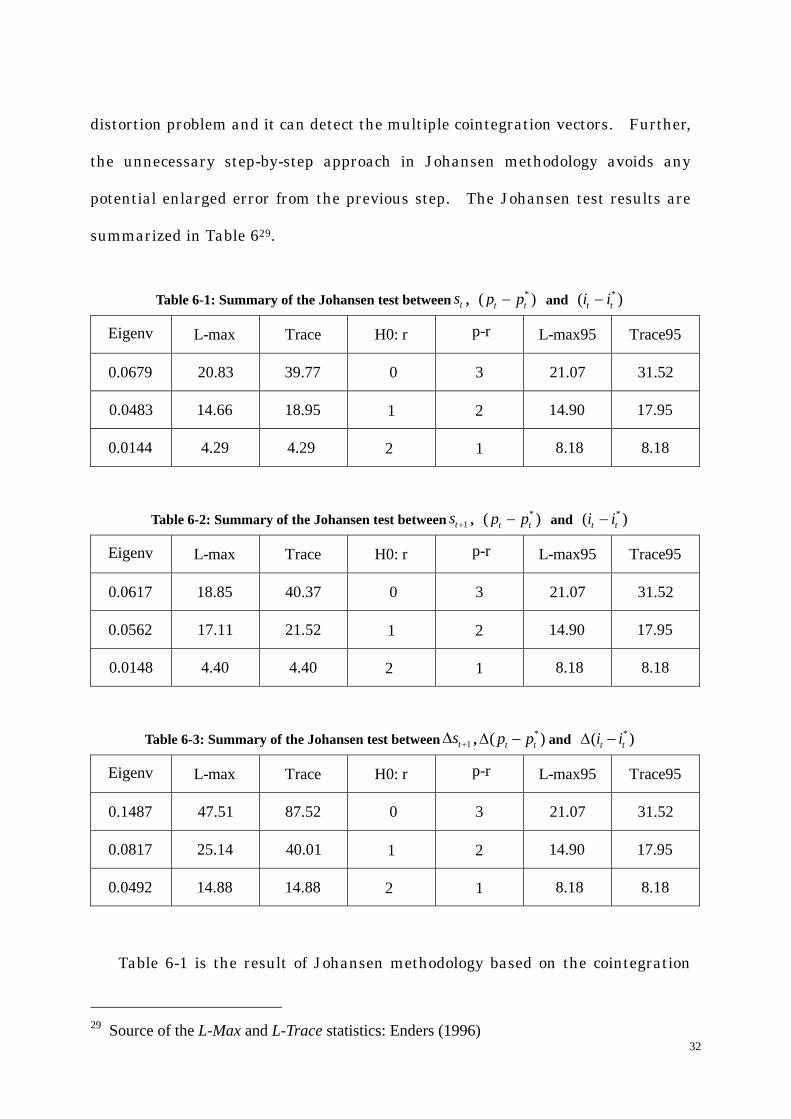
distortion problem and it can detect the multiple cointegration vectors. Further,
the unnecessary step-by-step approach in Johansen methodology avoids any
potential enlarged error from the previous step. The Johansen test results are
summarized in Table 629.
Table 6-1: Summary of the Johansen test between , ts *( )t tp p− and *( )t ti i−
Eigenv L-max Trace H0: r p-r L-max95 Trace95
0.0679 20.83 39.77 0 3 21.07 31.52
0.0483 14.66 18.95 1 2 14.90 17.95
0.0144 4.29 4.29 2 1 8.18 8.18
Table 6-2: Summary of the Johansen test between 1ts + , *( )t tp p− and ( ) *t ti i−
Eigenv L-max Trace H0: r p-r L-max95 Trace95
0.0617 18.85 40.37 0 3 21.07 31.52
0.0562 17.11 21.52 1 2 14.90 17.95
0.0148 4.40 4.40 2 1 8.18 8.18
Table 6-3: Summary of the Johansen test between 1ts +∆ , *( )t tp p∆ − and *( )t ti i∆ −
Eigenv L-max Trace H0: r p-r L-max95 Trace95
0.1487 47.51 87.52 0 3 21.07 31.52
0.0817 25.14 40.01 1 2 14.90 17.95
0.0492 14.88 14.88 2 1 8.18 8.18
Table 6-1 is the result of Johansen methodology based on the cointegration
29 Source of the L-Max and L-Trace statistics: Enders (1996)
32

analysis between the contemporaneous exchange rate, price and interest rate
differentials, which is the method adopted by most of the other researchers.
Table 6-2 gives the cointegration analysis between the expected future exchange
rate, price and interest rate differentials while Table 6-3 is the result of the
modified model, i.e., the differenced model of equation (19). Comparing the
results in the three sub-tables, we conclude that the effect of this modification is
significant. Only Table 6-3, i.e., the sub-table with the modified model can yield
the cointegration relationship30.
3.3.3.
1te
The error correction model (ECM)
According to Granger representation theorem, cointegration and error
correction are equivalent representations, i.e. cointegration implies error
correction and vice versa. The next stage involves the error correction model for
the VAR system (20), which should have the form of:
1 1 1 1( )ts α β+∆ ∆ = + Φ +Π + (23-1)
*2 2 2( )t 2tp p α β∆∆ − = + Φ +Π + e
3t
1)ti −
3
(23-2)
(23-3) *3 3 3( )ti i eα β∆∆ − = + Φ +Π +
where * *1 1 1( ) (t p t t i ts p p iα β β− − −Φ = ∆ − − ∆ −∆ − ∆ −∆
1( ) ( )n sn t pn t t is p pβ β+= ∆ ∆ + ∆ ∆ −∆ + ∆ ∆∑ ∑ ∑
31,
* *( ), 1, 2,n t ti i nβΠ −∆ =
1te , and e2te 3t =white-noise disturbances which may be correlated with each
other and α , β are parameters.
represents the real error Φ 1tε − in equation (21). Since /1tε − is the
30 In Table 6-1 and Table 6-2, L-Max and L-Trace contradicts each other in that only the latter rejects cointegration. We should pin down the number of cointegration vectors and therefore we conclude that there is no cointegration. 31 pβ and iβ are the cointegrationg vectors given by equation (21).
33

estimation of deviation from long-run equilibrium in period ( 1)t − , as proposed by
Engle and Granger, it is possible to use the saved residuals /1{ t }ε −
1 1
obtained from
the regression of equation (21) as an instrument for the expression . Based on
this substitution, the error-correction model (ECM) is estimated to be:
Φ
1t
te
t
2t
/1( ) 0.00013 0.76179ts eε+ t−∆ ∆ = − − +Π + (24-1)
(-7.8129) (0.00000)
* /1 2( ) 0.012055t tp p ε −∆∆ − = − +Π + (24-2) 2
(-0.65688) (0.5118)
(24-3) * /1 3( ) 0.0001 0.033t ti i eε −∆∆ − = + +Π + 3
(1.02725) (0.3052)
The value in the parenthesis under each equation shows t-value and the
significance level. In equation (24.1), the error-correction term is of highly
significance level. This suggests that the future change of exchange rate is strongly
determined by the long-run equilibrium. Further, the sign of the error-correction
terms 1tε − in equation (24.2) is not consistent with the theory, making (24.2) looks
more like error-amplifying rather than error-correction. The significance level,
however, is very low. This indicates that the differenced price level is rather rigid
and does not respond to the deviation from the long-run equilibrium level much.
3.3.4. Causality test and innovation accounting
In VAR analysis, we say that does not Granger-cause q if the lagged
values of do not appear in the equation for , that is, the current and lagged
do not help to predict the future value of . The null hypothesis that does not
Granger-cause can be tested by doing a joint F-test: regress on both the
lagged and the lagged and see the significance of the coefficient of lagged .
1tq
1tq
t
2tq 1tq
1tq
2tq 1tq
2tq 2tq
1q 2tq
34

The following part of this section investigates the Granger causality relationship
among the three variables in the exchange rate determination model: 1ts +∆ ,
*( )t tp p∆ − and while performing the innovation accounting. *( t ti i∆ −
∆
)
Based on the VAR system (20), we first conduct the Granger causality test. The
F-test and the corresponding significance level are reported in Table 7.
Table 7: Summary of Granger-Causality Tests
variable 1ts + *( )t tp p∆ − *( )t ti i∆ −
1ts +∆ 21.57 0.000 0.024 0.976 0.722 0.487
4.121 0.017 7.184 0.001 5.234 0.006
*( )t ti i∆ − 1.741 0.177 0.361 0.697 2.622 0.074
*( )t tp p∆ −
Table 7 shows that Granger-causes only itself; 1ts +∆ *( t ti i )∆ − also roughly
Granger-causes only itself, while *( t t )p p∆ − Granger-causes all the three variables.
To further identify the different roles *( t t )p p∆ − and *( t ti i )∆ − play in the model
of exchange rate determination, we can decompose the forecast error variance. The
forecast error variance decomposition tells us the proportion of the movements in a
sequence due to its own shocks versus shocks to the other variables.
We use the variance matrix in the VAR system (20) to obtain 1-step ahead
through 24-step ahead forecast errors. Appendix 4 shows the first five impulses,
together with the variance decomposition. To measure all responses in terms of
standard deviations, we depict the following impulse response functions.
35

Figure 6-1
Plot of Responses To ds
0 2 4 6 8 10 12 14 16 18 20 22-0.2
0.0
0.2
0.4
0.6
0.8
1.0dsddpddi
Figure 6-2
Plot of Responses To ddp
0 2 4 6 8 10 12 14 16 18 20 22-0.25
0.00
0.25
0.50
0.75
1.00dsddpddi
36
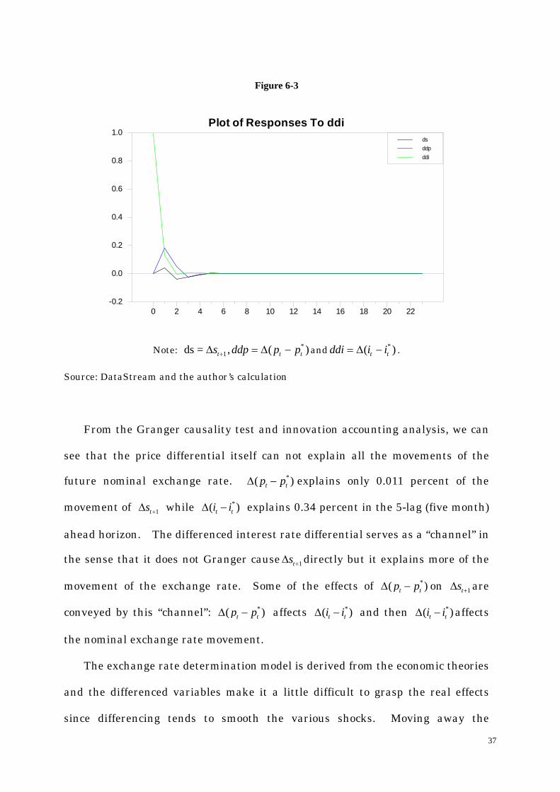
Figure 6-3
Plot of Responses To ddi
0 2 4 6 8 10 12 14 16 18 20 22-0.2
0.0
0.2
0.4
0.6
0.8
1.0dsddpddi
Note: and*1ds = , ( )t ts ddp p p+∆ = ∆ − t
*( )t tddi i i= ∆ − .
Source: DataStream and the author’s calculation
From the Granger causality test and innovation accounting analysis, we can
see that the price differential itself can not explain all the movements of the
future nominal exchange rate. *( t t )p p∆ −
)
ts
explains only 0.011 percent of the
movement of while explains 0.34 percent in the 5-lag (five month)
ahead horizon. The differenced interest rate differential serves as a “channel” in
the sense that it does not Granger cause
1ts +∆ *( t ti i∆ −
1+∆ directly but it explains more of the
movement of the exchange rate. Some of the effects of *( )t tp p∆ − on 1ts +∆ are
conveyed by this “channel”: *)t t( p p∆ − affects *( t ti i )∆ − and then affects
the nominal exchange rate movement.
*( ti∆ − )ti
The exchange rate determination model is derived from the economic theories
and the differenced variables make it a little difficult to grasp the real effects
since differencing tends to smooth the various shocks. Moving away the
37
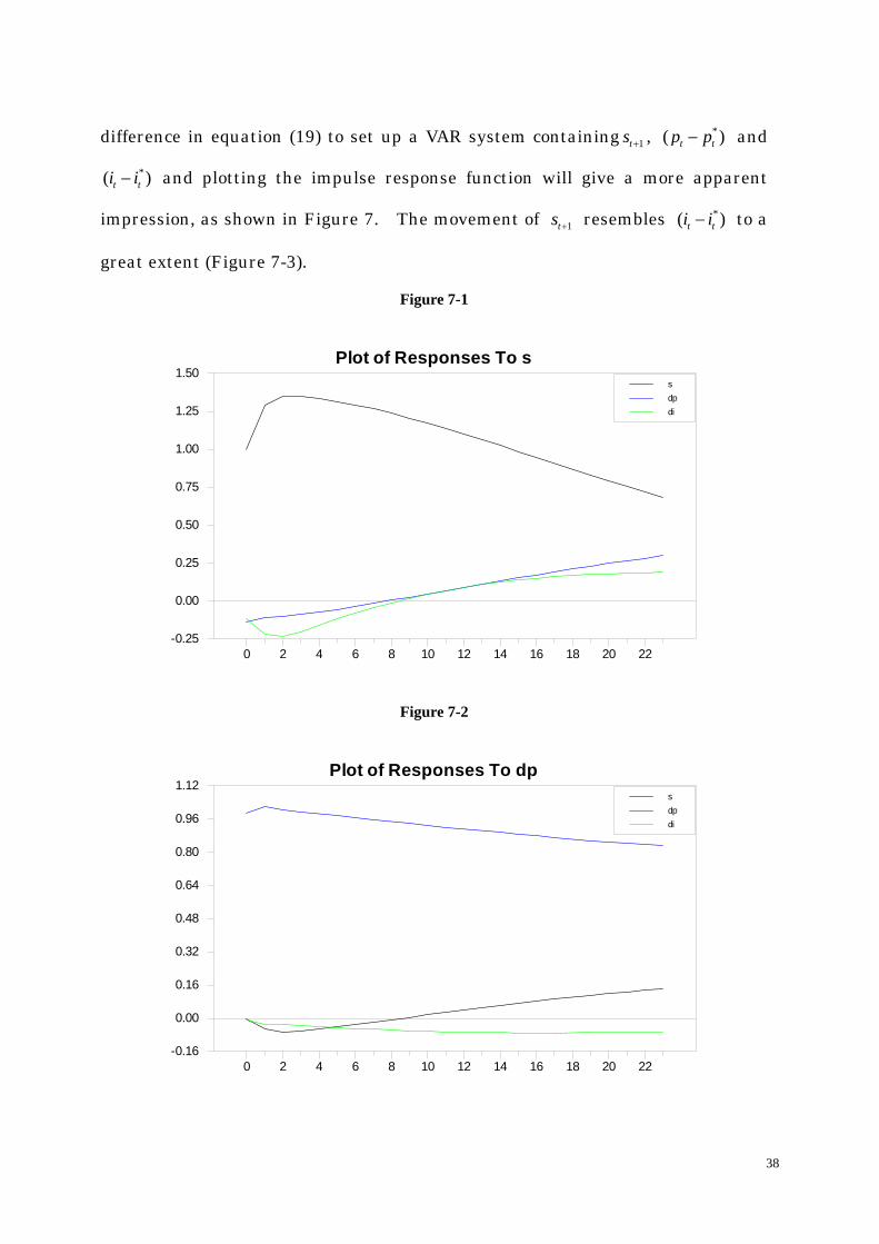
difference in equation (19) to set up a VAR system containing , 1ts +*( t t )p p− and
and plotting the impulse response function will give a more apparent
impression, as shown in Figure 7. The movement of
*( t ti i− )
1ts + resembles to a
great extent (Figure 7-3).
*( t ti i− )
Figure 7-1
Plot of Responses To s
0 2 4 6 8 10 12 14 16 18 20 22-0.25
0.00
0.25
0.50
0.75
1.00
1.25
1.50sdpdi
Figure 7-2
Plot of Responses To dp
0 2 4 6 8 10 12 14 16 18 20 22-0.16
0.00
0.16
0.32
0.48
0.64
0.80
0.96
1.12sdpdi
38

Figure 7-3
Plot of Responses To di
0 2 4 6 8 10 12 14 16 18 20 22-0.75
-0.50
-0.25
0.00
0.25
0.50
0.75
1.00
1.25sdpdi
Note: and di*1s = , ( )t ts dp p p+ = − t
*( )t ti i= −
Source: DataStream and the author’s calculation
Moreover, considering the interest rate differential is small in value and
differencing it may cause it to appear white noise32, its effect tends to be
underestimated in model (19). Granger causality test between , 1ts +*( t t )p p− and
yields a different result, as is shown in Table 8. *( t ti i− )
Table 8: Summary of Granger Causality Tests
variable 1ts + *( )t tp p− *( )t ti i−
1ts + 6599 0.000 2.286 0.103 7.41 0.001
*( )t tp p− 3.45 0.033 61750 0.000 5.86 0.003
*( )t ti i− 4.832 0.009 1.423 0.243 1229 0.000
32 The mean of is . *( )t ti i∆ − 0.000201
39

The value in italic forms shows the significance level. As indicated from the
Table 8, in the 5 percent significance level, the price differential *( )t tp p−
*( )t ti i
Granger-cause both and interest rate differential ; 1ts +*( )t ti i− −
Granger-causes and it explains 9.715 percent of the 12-lag ahead forecast
error of , leaving
1ts +
1ts +*( t )tp p− only account for 0.772 percent in the same period.
Therefore, the interest differential seems more essential in the determination of
exchange rate movement in the short run.
40

4. Long-Run Analysis (Year 1870~2003)
4.1.
1+
The CHEER Model of Exchange Rate Determination
Analysis of Chapter 3 is based on the monthly data in the post floating period
spanning 31 years (from 1973 to 2004); this chapter employs longer data span,
which is annual data spanning from year 1870 to 2003. This data set contains
the exchange rate, the CPI index and the long-term interest rates for U.S and
Japan33.
4.1.1. Unit root tests
The unit root tests for PPP and UIP are performed in the first step to
determine whether they hold. Here we also assume perfect foresight, i.e.,
in UIP hypothesis. As shown in equation (9) and (15), the unit root
tests can be conducted by testing the null hypothesis that
1( )t t tE s s+ =
0γ = . The test
statistics are abbreviated as Table 9.
Table 9: Unit root tests
Test DF PP ADF34
γ in PPP equation -3.3485 -3.2633 -1.61463
γ in UIP equation -8.1145 -8.3654 -3.19689
The 5 percent critical value for the null that 0γ = is -2.883 and all the
33 Long-term interest rates are U.S 10 year government bond yield and Japanese 7 year government bond yield. The maturities are different because no other long-run rate is available. 34 The lags in ADF equations are 8.
41

absolute value of the statistics reported in Table 9 exceed this except the ADF
statistics for PPP, which is -1.61463. As Campbell and Perron (1991) pointed out,
nonrejection of the unit root hypothesis may be due to the existence of structural
breaks. From year 1870 to 2003, at least two structural breaks occurred. As
Figure 8 shows, one is year 1945, in which the yen depreciated more than 200
percent (from 4.29 to 15). The other notable break is year 1970, in which the yen
began to appreciate sharply due to the oil shock35.
Considering the existence of two structural breaks, we should detrend the
real exchange rate before performing the unit root tests. First, we regress:
0 1 1 1970 2 1985q a a t D D qtt L Lµ µ∧
= + + + +
where and are level dummies representing structural breaks in
year 1970 and 1985, respectively;
1970LD 1985LD
1µ and 2µ are coefficients of and , respectively; 1970LD 1985LD
t represents time and , are parameteres. 0a 1a
Then, we perform the unit root test on the detrended real exchange rate, qt∧
to regress:
810 1
qq qt t i t iiα γ β
∧ ∧∆ = + + ∑− −=
The estimated t-statistics for 0γ = is -3.1515, exceeding the 5 percent critical
value of -2.883. Therefore, we conclude that the null hypothesis of unit root can
be rejected and both PPP and UIP hold in the long run. The graph of nominal
and real exchange rate, changes in real exchange rate and interest rate
42
35 Year 1985 may be considered as another break for the advent of the Plaza Agreement. It is not necessary to deal with it here, however, since we have taken year 1970 as a break and we can view year 1985 as a point in the appreciation trend of yen.

differential are depicted in Figure 8,9,10 and 11.
Figure 8
Nominal and Real Exchange Rate (Yen/Dollar)
1870 1881 1892 1903 1914 1925 1936 1947 1958 1969 1980 1991 20020
100
200
300
400
500
600
700NOMINALREAL
Source: DataStream and the author’s calculation
Figure 9
Nominal and Real Exchange Rates for Yen (in logs)
1870 1880 1890 1900 1910 1920 1930 1940 1950 1960 1970 1980 1990 2000-1
0
1
2
3
4
5
6
7nominalrea;
Source: DataStream and the author’s calculation
43

Figure 10
Changes In Real Exchange Rate of Yen
1871 1883 1895 1907 1919 1931 1943 1955 1967 1979 1991 2003-1.5
-1.0
-0.5
0.0
0.5
1.0
1.5
Source: DataStream and the author’s calculation
Figure 11
Nominal Interest DIfferential(Japan-U.S) in log value
1870 1882 1894 1906 1918 1930 1942 1954 1966 1978 1990 2002-0.06
-0.04
-0.02
0.00
0.02
0.04
0.06
0.08
0.10
Source: DataStream
44

4.1.2.
p
The nominal exchange rate determination model
The PPP and UIP can be written in the following equations:
*t t ts p p η= − + (25)
*1t t t ts s i i iη+ − = − + (26)
where pη and iη are residuals.
Regress equation (25) and (26) and we obtain:
*5.748 1.017( )t ts p= + − tp
)
(107.0) (71.7)
*1 0.026 0.7645( )t t t ts s i i+ − = + −
(1.08) (1.005)
The t-statistics are shown in the parenthesis and the null hypothesis of
coefficients of *( t tp p− and ( equal to unity cannot be rejected*t ti i− )
t
36.
By substituting (25) into equation (26), we can obtain the following equation:
* *1 ( ) ( )t t t t ts p p i i ε+ = − + − + (27)
where t p iε η η= + .
Equation (27) is the determination of nominal exchange rate in the long run.
It can be interpreted that the future nominal exchange rate is determined by the
current price and interest rate differentials. In this equation, three variables
are concerned, , 1ts +*( t t )p p− and ( *
t ti i )− . According to equation (27), we can set
up a VAR model as:
* *10 1 1 1 1
0 0 0( ) ( )
p p p
t m t m m t m m t m tm m m
s a b s c p p d i i e− −= = =
= + + − + − +∑ ∑ ∑ −
(28-1)
45
36 The F-statistics of the null that the coefficient equal to 1 is tested to be 1.3576 and 0.09183 in equation (25) and (26) respectively, which is less than the 1 percent critical value 6.63.

* *20 2 2 2 2
0 0 0
( ) ( ) ( )p p p
t m t m m t m m t m tm m m
*p p a b s c p p d i i e− −= = =
− = + + − + − +∑ ∑ ∑
* *30 3 3 3 3
0 0 0
( ) ( ) ( )p p p
t m t m m t m m t m tm m m
i i a b s c p p d i i e− − −= = =
− = + + − + − +∑ ∑ ∑
( 1,2,3)ite i
−
*
(28-2)
(28-3)
=
3p =
1t+*( )t tp p−
* * /1 ( ) ( )t p t t i t t ts p p i iα β β ε+ = + − + − +
value Std Error t statistics−
where a, b, c, and d are parameters, and are error-terms.
The lag length in system (28) is determined using AIC and SBC criteria,
whose value is the smallest when 3 lags are used. Therefore, we set .
4.2. Engle-Granger Cointegration Test and ECM
We also adopt Engle-Granger approach to test the cointegration relationship
among the three variables concerned in equation (27): s , and ( )*t ti i− .
Pretests of the order of their integration indicate that they are all I(1) processes.
The next step entails regressing on the following equation to get the long-run
equilibrium relationship.
(29)
where /tε is the estimated error. The result of the regression is reported in
Table 10.
Table 10: Regression Results in the Long Run
coefficient significance
α 5.7580 0.0433 133.001 0.000
pβ 1.0519 0.012 87.8757 0.000
iβ 10.8902 1.0525 10.3468 0.000
Just the same as equation (22) in Section 3.3.1, we regress the following
equation to know the t-statistics of 1α .
46

/ /1 1t t eε α ε −∆ = + t
t
(30-1)
/ / /1 1 1t t i t i eε α ε α ε− + −∆ = + ∆ +∑ (30-2)
where are white noise. te
The estimated t-statistics of 1α in (30.1) and (30.2) are -5.6731 and –3.4221,
respectively, and both exceeding the critical values for the null of no cointegration
at 5 percent level (-3.17 with lags and –3.37 without lags respectively). Moreover,
by changing the regression order, i.e., changing the left side variable in equation
(29) do not lead to different results. The t-values of the estimated errors both
exceed the critical value in the Engle-Granger no cointegration table. Therefore,
we can reject the null of no cointegration.
After the cointegration test, we then estimate the ECM, which should have
the form as the following if we substitute /1tε − with the real error term 1tε − ,
(31-1) /1 1 1 1 1t ts α β ε+ −∆ = + +Π + 1te
2t * /2 2 1 2( )t tp p α β ε −∆ − = + +Π + e
3t
(31-2)
(31-3) * /3 3 1 3( )t ti i eα β ε −∆ − = + +Π +
where
* *1 1 1( ) (p t t i t t )p p iβ βΠ = ∆ − + ∆ − i *
2 2 1 2 ( ), s t i ts iβ β+Π = ∆ + ∆ − ti*
3 3 1 3 ( ), s t p ts pβ β+Π = ∆ + ∆ − tp ,
, and e white-noise disturbances which may be correlated with each
other; and
1te 2te 3t =
α , β are parameters.
System (31) is estimated to be:
/1 0.007 ( 0.0260)t ts eε+ −∆ = + − + Π +1 1 1t
2t
(32-1)
(0.385) (-0.296)
* /1 2( ) 0.021 0.165t tp p eε −∆ − = + + Π + (32-2)
(1.818) (3.130)
* /1 3( ) 0.0004 0.0113t ti i eε −∆ − = − + + Π + 3t (32-3)
(-0.359) (2.432)
47

` The value in the parenthesis below each estimated coefficient is the
corresponding t-value. Careful examination of system (32) would reveal that if
/1tε − is positive, i.e., if is larger than the long-run equilibrium level, then the
ECM will make it to decrease while
1ts +
*( t)p p− and ( to increase, making it
possible to restoring to the equilibrium. Therefore, different from the short run
ECM, the long-run ECM is stable.
*ti i− )
Although the ECM is stable in the long run, the coefficient of /1tε − in equation
(32-1) is not significant, implying the exchange rate does not respond to the
long-run deviation. What makes this coefficient be insignificant? We expect to
answer this question by performing the Granger causality tests to reveal the
intrinsic relationship between the variables in system (28).
4.3. Granger Causality and Johansen Methodology
Granger causality test between 1ts + , *( )t tp p− , *( t ti i )− are helpful to further
reveal the roles each variable plays in the long-run nominal exchange rate
determination. The joint F-statistics and the significance levels of system (28)
are reported in Table 11.
Table 11: Granger Causality Tests for the Long Run
variable 1ts + *( )t tp p− *( )t ti i−
1ts + 89.91 0.000 12.87 0.000 0.042 0.989
*( t t )p p− 16.91 0.000 154.13 0.000 1.482 0.223
*( )t ti i− 2.300 0.081 1.696 0.172 59.404 0.000
48

Table 11 indicates that at 5 percent significance level, 1ts + and *( t t )p p− both
Granger-cause themselves and each other; *( t ti i )− Granger-causes only itself and
is not Granger-caused by any of the other two. These results imply that the
interest rate differential is not an endogenous variable in the system of
exchange rate determination.
*( t ti i− )
)
The exogenous property of interest rate differential raises a serious question
of system (28), i.e., is it appropriate to include *( t ti i− in the VAR system?
Because the likely ratio test can determine whether a variable should be included,
we perform the likely ratio test of *( t ti i )− . Begin with PPP equation (25), suppose
that should not be included, the likely ratio statistics4
*( t p t pp o
i i− −=
−∑
04
)
)
37 is 8.831921
with significance level , less than the 5 percent critical value of
. Therefore, the null hypothesis of exclusion of ( can not be
rejected.
0.54812587
18.307 *t ti i−
The Granger Causality tests and likely ratio tests both questions the
hypothesis of CHEER in the long run. Because CHEER approach is often tested
with the cointegration method, we proceed to use Johansen methodology, the
more powerful cointegration test, to reinvestigate the cointetgration relationship.
As stated in Section 3.3.2., Johansen methodology circumvents the small sample
size distortion problem and it can detect the multiple cointegration vectors.
Further, the unnecessary step-by-step approach in Johansen methodology avoids
any potential enlarged error from the previous step.
According to the CHEER model of equation (27), we perform the Johansen
49
37 The test equation is similar with equation (15). Here the number of restrictions is 10 (lag 0,1,2,3,4 in each equation) and the unrestricted model contains 12 coefficients.

test to detect the cointegration between the exchange rate, price and interest rate
differentials. The Johansen test results are summarized in Table 12.
Table 12: Johansen Cointegration Test
Eigenv L-max Trace H0: r p-r L-max95 Trace95
0.1286 17.89 27.22 0 3 21.07 31.52
0.0510 6.80 9.33 1 2 14.90 17.95
0.0192 2.52 2.52 2 1 8.18 8.18
Table 12 indicates that the null hypothesis of no cointegration vector among
, 1ts +*( t)p p− and can not be rejected either by the L-max or Trace
statistics. Therefore, the CHEER approach fails in the long run and the
exchange rate determination model is only represented by PPP.
*( ti i− )
)
The fact of CHEER hypothesis in the long run is a surprise because we have
found cointegration in the short run and many economic hypotheses tends to hold
better in the long run. We can explain the puzzle from the history of financial
markets. Financial markets did not develop well until the past twenty years and
its role in the exchange rate determination is not apparent if we view it in a very
long data span. If we test CHEER hypothesis using the recent data, the interest
rate differential tends to become more significant because of its notable size. In
short, the 130 years is too long and the effect of financial market in exchange rate
determination in recent years is “diluted”.
The forecast error decomposition also suggests that the price differential
*( t tp p− is the dominant factor in the determination of 1ts + . In the 5-lag ahead
forecast horizon, *( t t )p p− explains about 10 percent of the error of , while 1ts +
50

*( t ti i− ) explains about 0.1 percent (See Appendix 5).
Figure 12 depict the impulse response functions. The responses of 1ts +
resembles that of in the short run; however, it resembles *( ti i− ) )*( p p− in the
long run and the price differential affects it more in magnitude.
Figure 12-1
Plot of Responses To s
0 2 4 6 8 10 12 14 16 18 20 22-0.4
0.0
0.4
0.8
1.2
1.6
2.0
2.4
2.8sdpdi
Figure 12-2
Plot of Responses To dp
0 2 4 6 8 10 12 14 16 18 20 22-0.25
0.00
0.25
0.50
0.75
1.00
1.25
1.50sdpdi
51

Figure 12-3
Plot of Responses To di
0 2 4 6 8 10 12 14 16 18 20 22-0.6
-0.4
-0.2
-0.0
0.2
0.4
0.6
0.8
1.0sdpdi
Note: and*1s = , ( )t ts dp p p+ = − t
*( )t tdi i i= − .
Source: DataStream and the author’s calculation
52

5. Conclusion
The major conclusion of this paper is that the validity of the exchange rate
model combing PPP and UIP strongly depends on the data span. Either failure
of PPP or UIP will lead to no cointegration between the future exchange rate,
price and interest rate differentials without appropriate modification of the
cointegration variables. The cointegration relationship does not necessarily
exist, however, even when both PPP and UIP hold. Further, in the VAR model of
exchange rate determination, the roles of price and interest rate differentials play
in the exchange rate determination are remarkably different between the short
run and the long run.
In the short-run analysis during the floating period with monthly data, PPP
fails and UIP holds. The variables in the CHEER approach are differenced to
improve the test power of the cointegration analysis. With this modification,
cointegration is found between the future exchange rate, price and interest rate
differentials. The likely ratio test indicates that the interest rate differential is
an endogenous variable and it explains more of the movement of the future
exchange rate. The Granger causality tests indicates that although both the
price and interest differentials Granger-cause the future nominal exchange rate,
some effects of the price differential is transmitted by the interest differential,
making the latter explain more forecast variance of the exchange rate. The
coefficients in ECM are significant; however, because of the price rigidity, the
ECM is not stable in the short run.
In the long-run analysis using yearly data of longer than one century, both
UIP and PPP hold. The interest rate differential becomes an exogenous variable 53
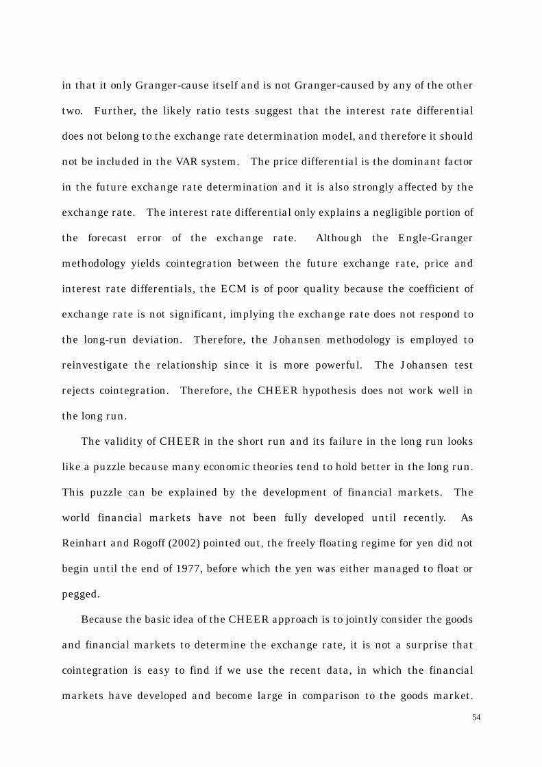
in that it only Granger-cause itself and is not Granger-caused by any of the other
two. Further, the likely ratio tests suggest that the interest rate differential
does not belong to the exchange rate determination model, and therefore it should
not be included in the VAR system. The price differential is the dominant factor
in the future exchange rate determination and it is also strongly affected by the
exchange rate. The interest rate differential only explains a negligible portion of
the forecast error of the exchange rate. Although the Engle-Granger
methodology yields cointegration between the future exchange rate, price and
interest rate differentials, the ECM is of poor quality because the coefficient of
exchange rate is not significant, implying the exchange rate does not respond to
the long-run deviation. Therefore, the Johansen methodology is employed to
reinvestigate the relationship since it is more powerful. The Johansen test
rejects cointegration. Therefore, the CHEER hypothesis does not work well in
the long run.
The validity of CHEER in the short run and its failure in the long run looks
like a puzzle because many economic theories tend to hold better in the long run.
This puzzle can be explained by the development of financial markets. The
world financial markets have not been fully developed until recently. As
Reinhart and Rogoff (2002) pointed out, the freely floating regime for yen did not
begin until the end of 1977, before which the yen was either managed to float or
pegged.
Because the basic idea of the CHEER approach is to jointly consider the goods
and financial markets to determine the exchange rate, it is not a surprise that
cointegration is easy to find if we use the recent data, in which the financial
markets have developed and become large in comparison to the goods market.
54

For the same reason, supportive evidence of CHEER becomes difficult to find
when we use the long-run historical data, in which the world financial markets
are not fully developed. In this paper, the short-run and long-run data span the
past 30 years and the 130 years, respectively. The effect of financial markets in
the long run is “diluted” by the 100 years (from 1870 to 1970s) of the long-run
data. Therefore, we expect that the CHEER approach will be supported with
new future data.
The findings of this paper have important policy implications for monetary
authorities. In the short run, it is more effective to control the interest rate to
reduce the exchange rate volatility because the interest rate differential explains
more of the forecast decomposition. In the long run, however, the price level
becomes a dominant factor in the determination of the exchange rate. Therefore,
the control of money supply should be given high priority because the interest
rate differential becomes exogenous and it only explains a negligible portion of
the long-run exchange rate movement.
55

Appendix
.
Appendix 1: Program Description
Software used:
I have used the following software to test the hypotheses, estimate the
equations and depict the graphs.
1. Regression Analysis of Time Series (RATS) of version 5.11, Estima Company
(2002).
2. Cointegration Analysis of Time Series (CATS) of version 1.03; Estima
Company (2002).
Software Manual:
I have consulted the following three books to write and run the programs.
1. “RATS User’s Guide” (version 5, 2002), Estima Company.
2. “Rats Reference Manual” (version 5, 2002), Estima Company.
3. “RATS Handbook For Econometric Time Series” (1996), Water Enders, John
Wiley & Sons, Inc.
56

Appendix 2: Data Source and Description
Data Source:
Short Run( Jan.1973~ Jun. 2004, monthly): DataStream and the author’s
calculation (data on the first day of each month)
Long Run(Year 1870~Year 2003,annually): Global Financial Data, Incorporation.
Directory of “Sample Data Access” on http://www.globalfindata.com/ (Sections of
“Commodity Prices”, “Exchange Rates”, and “Interest Rates” of U.S. and Japan).
Data Description:
S: yen/dollar exchange rate (New York market buying rates for the short run;
close rates on the last day of each year for the long run).
IJ: Japanese nominal interest rate level (euro rates in London market for the
short run; 7-year government bond rate for the long run);
IU: U.S. nominal interest rate level (euro rates in London market for the short
run; 10-year government bond rate for the long run);
PU: U.S. consumer price index (CPI);
PJ: Japanese consumer price index;
INFU: U.S. inflation level (calculated from “PU”);
INFJ: Japanese inflation level (calculated from “PJ”);
RIU: U.S real interest level (calculated from “IU” and “INFU”);
RIJ: Japanese real interest level (calculated from “IJ” and “INFJ”).
57

Appendix 3: Data Summary
Appendix 3.1: Short Run
Series Obs Mean Std Error Minimum Maximum
S 377 176.567533 67.484020 83.690000 305.67000IU 353 0.070099 0.036694 0.010313 0.193750IJ 311 0.037805 0.032370 -0.005000 0.144375PU 376 219.346888 78.871551 78.681454 347.01170PJ 376 155.058245 30.585180 67.300000 186.60000INFJ 376 0.034114 0.050785 -0.016000 0.251000INFU 376 0.049125 0.032070 0.011000 0.148000RIU 351 0.024031 0.025832 -0.044500 0.090375RIJ 309 0.022462 0.020216 -0.042250 0.069125
Appendix 3.2: Long Run
Series Obs Mean Std Error Minimum Maximum
S 134 107.617443 140.804934 0.902700 360.0000PJ 134 23.806538 35.651962 0.018500 101.3000PU 134 40.087280 49.057558 6.762000 184.3000IJ 134 0.058510 0.021692 0.005400 0.148200IU 134 0.045743 0.023343 0.016700 0.139800
58

Appendix 4: Short-Run Forecast Error
Appendix 4.1: 5 Step Ahead Forecast Error
.
1
* *1
Responses to Shock in
Entry ( ) ( ) 1 0.0269163 -0.0003734 0.0006010 2 0.0102160 -0.0007288
t
t t t t
s
s p p i
+
+ ti
∆
∆ ∆ − ∆
-0.0006404 3 0.0011473 -0.0000850 -0.0005743 4 -0.0004385 0.0001329 -0.0002220
−
5 -0.0001759 0.0000187 -0.0000339
t ti i−
t ti−
*
* *1
Responses to Shock in ( )
Entry ( ) ( ) 1 0.0000000 0.0046116 -0.0001098 2 0.0002941
t t
t t t
p p
s p p+
∆ −
∆ ∆ − ∆
0.0002763 -0.0003239 3 -0.0000268 -0.0009620 0.0001913 4 -0.0000195 -0.0000973 0.0001075 5 -6.6473524e-06 0.0002028 -0.0000349
*
* *1
Responses to Shock in ( )
Entry ( ) ( ) 1 0.0000000 0.0000000 0.0082958 2 0.0011300 0.0008391 0.0
t t
t t t
i i
s p p i+
∆ −
∆ ∆ − ∆
010996 3 -0.0010072 0.0002299 -0.0000398 4 -0.0007153 -0.0001086 0.0000319 5 -0.0001795 -0.0000391 0.0000532
59

Appendix 4.2: Forecast Error Decomposition
1
* *1
Decomposition of Variance for Series
Step Std Error ( ) ( ) 1 0.026916326 100.000 0.000 0.000 2 0.028813520 99.836 0.010 0
t
t t t t
s
s p p i
+
+ ti
∆
∆ ∆ − ∆ −
.154 3 0.028853951 99.714 0.010 0.275 4 0.028866154 99.653 0.011 0.336 5 0.028867249 99.649 0.011 0.340
t
*
* *1
Decomposition of Variance for Series ( )
Step Std Error ( ) ( ) 1 0.004626714 0.651 99.349 0.000 2 0.004766341 2.952 93.949
t t
t t t t
p p
s p p i+
∆ −
i∆ ∆ − ∆ −
3.099 3 0.004868629 2.859 93.947 3.193 4 0.004872624 2.929 93.833 3.238 5 0.004877036 2.925 93.837 3.238
*
* *1
Decomposition of Variance for Series ( )
Step Std Error ( ) ( ) 1 0.008318276 0.522 0.017 99.461 2 0.008421267 1.088 0.165
t t
t t t t
i i
s p p i+
∆ −
ti∆ ∆ − ∆ −
98.748 3 0.008443089 1.545 0.215 98.240 4 0.008446750 1.612 0.231 98.156 5 0.008447058 1.614 0.233 98.153
.
60

Appendix 5: Long-Run Forecast Error Decomposition
1
* *1
Decomposition of Variance for Series
Step Std Error ( ) ( ) 1 0.189581258 100.000 0.000 0.000 2 0.309738550 93.
t
t t t t
s
s p p i
+
+ ti− −
192 6.789 0.019 3 0.432056884 88.129 11.849 0.021 4 0.551653765 88.619 11.343 0.037 5 0.654340285 90.030 9.869 0.101
*
* *1
Decomposition of Variance for Series ( )
Step Std Error ( ) ( ) 1 0.114828590 13.133 86.867 0.000 2 0.243369338 33.84
t t
t t t t t
p p
s p p i i+
−
− −
5 66.096 0.059 3 0.364040946 49.553 50.328 0.119 4 0.463896056 58.664 40.993 0.343 5 0.546091937 64.297 35.020 0.683
*
* *1
Decomposition of Variance for Series ( )
Step Std Error ( ) ( ) 1 0.010359720 0.353 0.375 99.272 2 0.011577120 0.492
t t
t t t t t
i i
s p p i i+
−
− −
1.463 98.045 3 0.012845670 1.522 2.139 96.340 4 0.013825069 2.737 2.572 94.692 5 0.014661782 4.417 3.185 92.398
61

References
Abuaf, Niso and Philippe Jorion (1990), “Purchasing Power Parity in the Long
Run,” Journal of Finance 45: 157-74.
Adler, Michael and Bruce Lehmann (1983), “Deviations from Purchasing Power
Parity in the Long Run,” Journal of Finance 38: 1471-87.
Akaike, Hirotugu (1974), “A New Look at the Statistical Model Modification,”
IEEE Transactions on Automatic Control, AC-19: 716-23.
Alexius, Annika(2001), “Uncovered Interest Parity Revisited,” Review of
International Economics 9(3): 505-17.
Baum, Christopher F., John T. Barkoulas, and Mustafa Caglayan (2001),
“Nonlinear Adjustment to Purchasing Power Parity in the post-Bretton Woods
Era,” Journal of International Money and Finance 20:379-99.
Bec, Frederique Melika Ben Salem, and Marine Carrasco (2004), “Test for
Unit-Root versus Threshold Specification with an Application to the PPP,”
Journal of Business & Economic Statistics 22 (4): 382-95.
Black, Fisher (1986), “Noise,” Journal of F nance 41: 529-43. i
f
Campbell, John Y. and Pierre Perron (1991), “Pitfalls and Opportunities: What
Macroeconomists Should Know about Unit Roots,” NBER Macroeconomic
Annual: 143-201.
Campbell, John Y. and Richard H. Clarida (1987), “The Dollar and Real Interest
Rates,” Carnegie-Rochester Con erence Series on Public Policy 27: 103-40.
Caporale, Guilielmo, Sarantis Kalyvitis and Nikitas Pettis (2001), “Testing PPP
and UIP in a FIML Framework: Some Evidence for German and Japan,”
Journal of Policy Modeling 23: 637-650.
62

Cassel, Gustav (1921), “The World’s Monetary Problems,” London: Constable.
Cavallo, Michele and Fabio Ghironi (2002), “Net Foreigh Assets and the
Exchange Rate: Redux Revived,” Journal of Monetary Economics 49:
1057-1097.
Cheng, Benjamin S. (1999), “Beyond the Purchasing Power Parity: Testing for
Cointegration and Causality between Exchange Rates, Prices, and Interest
Rates,” Journal of International Money and Finance (18): 911-924.
Coakley, Jerry, Robert P. Flood, and Mark P. Taylor (2003), “Testing Long-Run
Relative Purchasing Power Parity,” mimeo, University of Warwick.
De Long, J. Bradford, Andrei Shleifer, Lawrence H. Summers, and Robert J.
Waldman (1990), “Noise Traders Risk in Financial Markets,” Journal of
Political Economy 98: 703-38.
Dornbush, Rudiger (1976), “Expectations and Exchange Rate Dynamics,” Journal
of Political Economy 84: 1161-76.
,
Edison, Hali J.(1987), “Purchasing Power Parity in the Long Run,” Journal of
Money Credit and banking 19: 376-87.
Enders, Walter (1995), Applied Econometric Time Series, John Wiley & Sons, Inc.
—— (1996), “RATS Handbook For Econometric Time Series”, John Wiley & Sons,
Inc.
Engel, Charles (1996), “The Forward Discount Anomaly and the Risk Premium: A
Survey of Recent Evidence,” NBER Working Papers.
Engel, Charles and James C. Morley (2001), “The Adjustment of Prices and the
Adjustment of Exchange Rate,” NBER Working Papers.
Engel, Charles and John H. Rogers (1996), “How Wide is the Border,” American
Economic Review 86: 1112-25.
63

Engle Robert F., David M. Lilien, and Russel P. Robins (1987), “Estimating Time
Varying Risk Premia in the Term Structure: The ARCH-M model,”
Econometrica 55: 391-407.
Engle, Robert E. and Clive-W.J. Granger (1987), “Cointegration and
Error-Correction: Representation, Estimation, and Testing,” Econometrica 55:
251-76.
Fisher, Eric (2001), “Purchasing Power Parity and Interest Parity in the
Laboratory,” Working Papers of Ohio State University, Department of
Economics.
Frankel, Jeffrey A. (1986), “International Capital Mobility and Crowding out in
the US Economy” in R.W. Hafer(Ed.), How Open is the US Economy?
Lexington: Lexington Books.
Frankel, Jeffrey A. and Andrew K.Rose (1996), “A Panel Project on Purchasing
Power Parity: Mean Reversion Within and Between Countries,” Journal of
International Economics 40:209-24.
Frenkel, Jacob A. (1978), “Purchasing Power Parity: Doctrinal Perspective and
Evidence from the 1920s,” Journal of International Economics 8: 169-91.
Froot, Kenneth A. and Kenneth Rogoff (1995), “Perspectives on PPP and
Long-Run Real Exchange Rates,” in Kenneth Rogoff and Gene Grossman
(eds.), Handbook of International Economics, Amsterdam: North-Holland.
Froot, Kenneth A., Michael Kim, and Kenneth Rogoff (1995), “The Law of One
Price Over 700 Years,” NBER Working Paper.
Gokcan, Aysun and Erdal Ozmen (2002), “Do PPP and UIP Need Each Other In a
Financially Open Economy? The Turkish Evidence,” ERC Working Papers in
Economics.
64

Granger, Clive W.J and Paul Newbold (1974), “Spurious Regression in
Econometrics,” Journal of Econometrics 2: 111-120.
Hansen, Lars Peter and Robert J. Hodrick (1980), “Forward Rates As Unbiased
Predictors of Future Spot Rates,” Journal of Political Economy 88: 829-53.
Hau, Harald (2000), “Exchange Rate Determination: The Role of Factor Price
Rigidities and Nontradeables,” Journal of International Economics 50(2):
1-16.
Im, Kyung So, M. Hashem Pesaran, and Yongcheol Shin (1997), “Testing for Unit
Roots in Heterogeneous Panels,” Working Papers Series, University of
Cambridge.
Isard, Peter (1977), “How Far Can We Push the ‘Law of One Price’?” American
Economic Review 67(5): 942-48.
Johansen, Soren and Katarina Juselius (1992), “Testing Structural Hypothesis in
a Multivariate Cointegration Analysis of the PPP and the UIP for the UK,”
Journal of Econometrics 53: 211-44.
Juselius, Katarina (1991), “Long-run relations in a well defined statistical model
for the data generating process: Cointegration analysis of the PPP and the
UIP relations for Denmark and Germany,” In Gruber, J (ed.): Econometric
Decision models: New Methods of Modeling and Applica ions. Springer
Verlag.
t
Juselius, Katarina and Ronald MacDonald (2000), “International Parity
Relationship between Germany and the United States,” Unpublished report,
European University Institute.
Kim, Jaebeom and Masao Ogaki (2004), “Purchasing Power Parity for Traded and
Non-Traded Goods: A Structural Error Correction Approach,” Monetary and
65

Economic Studies 22, 1-25.
Krasher, William S. (1980), “The ‘Peso Problem’ in Testing the Efficiency of
Forward Exchange Markets,” Journal of Monetary Economics 6: 269-76.
Levin, Andrew and Chien Fu Lin (1993), “Unit Root Tests in Panel Data: New
Results,” University of California, San Diego, Department of Economics
Working Paper.
Lewis, Karen K. (1989), “Changing Beliefs and Systematic Rational Forecast
Errors with Evidence from Foreign Exchange,” American Economic Review 79:
621-36.
Lothian, James R. and Mark P. Taylor (1997), “Real Exchange Rate Behavior: the
Problem of Power and Sample Size,” Journal of International Money and
Finance 16: 945-54.
——(1996), “Real Exchange Rate Behavior: the Recent Float from the Perspective
of the Past Two Centuries,” Journal of Political Economy 104: 488-510.
MacDonald, Ronald (2000), “Concepts to Calculate Equilibrium Exchange Rates:
An Overview,” Discussion Paper of Economic Research Group of the Deutsche
Bundebank.
Maddala, G.S. and Shaowen Wu (1999), “A Comparative Study of Unit Root Tests
with Panel Dataand a New Simple Test,” Oxford Bulletin of Economics and
Statistics 61: 631-52.
Mark, Nelson C. (2001), International Macroeconomics and Finance, Blackwell
Publisher Ltd, UK.
Mark, Nelson C. and Yangru Wu (1998), “Rethinking Deviations from Uncovered
Interest Parity: The Role of Covariance Risk and Noise,” Economic Journal
108: 1686-706.
66

Meese, Richard and Kenneth Rogoff (1988), “Was It Real? The Exchange
Rate-Interest Rate Differential Relation Over the Modern-Floating Period,”
Journal of Finance 43: 933-48.
Meredith, Guy and Menzie D. Chinn (1998), “Long-Horizon Uncovered Interest
Rate Parity,” NBER Working Papers.
Obstfeld, Maurice and Kenneth Rogoff (1995), Foundations of International
Macroeconomics, MIT press, London.
——(1996), “Exchange Rate Dynamics Redux,” Journal of Political Economy
103(3): 624-660.
Officer, Lawrence H. (1976), “The Purchasing-Power-Parity Theory of Real
Exchange Rates,” IMF Working Paper.
Ogaki, Masao (1999), “A Theory of Exchange Rates and the Term Structure of
Interest Rates,” Working Papers o Ohio State University, Department of
Economics.
f
i
Papell, David H. and Ruxandra Prodan (2004), “Long Run Purchasing Power
Parity: Cassel or Balassa- Samuelson?,” Working Paper of University of
Houston.
Phillips, Peter C.B. and Pierre Perron (1988), “Testing for a Unit Root in Time
Series Regression,” B ometrica 75: 335-46.
Reinhart, Carmen M. and Kenneth Rogoff (2002), “The Modern History of
Exchange Rate Arrangements: A Reinterpretation,” NBER Working Paper
Series.
Rogoff, Kenneth (1996), “The Purchasing Power Parity Puzzle,” Journal of
Economic Literature 34: 647-68.
Roll, Richard (1979), “Violations of Purchasing Power Parity and Their
67
68
Implications for Efficient International Commodity Markets,” in Sarnat M.
and Szego.G.P. (eds.), International Finance and Trade, Cambridge, Ballinger.
Samuelson, Paul A. (1964), “Theoretical Notes on Trade Problems,” Review of
Economics and Statistics 46: 145-54.
Sarno, Lucio and Mark P. Taylor (2002), “Purchasing Power Parity and the Real
Exchange Rate,” IMF Staff Papers 49(a): 65-105.
Schwarz, Gideon (1978) "Estimating the Dimension of a Model", Annals of
Statistics, 6, 461-464.
Sims, Christopher (1980), “Macroeconomics and Reality,” Econometrica 48: 1-49.
Stephens, Dominick (2004), “The Equilibrium Exchange Rate According to PPP
and UIP,” Reserve Bank of New Zealand, Discussion Paper.
Taylor, Mark P., David Peel, and Lucio Sarno (2001), “Nonlinear Mean-Reversion
in Real Exchange Rates: Towards a Solution to the Purchasing Power Parity
Puzzles,” International Economic Review 42: 1015-42.
Wu, Yangru (1996), “Are Real Exchange Rate Non-Stationary? Evidence from a
Panel-Data Test,” Journal of Money Credit and Banking 28:54-63.