international journal on advances in intelligent systems

The International Journal on Advances in Intelligent Systems is Published by IARIA.

ISSN: 1942-2679

journals site: http://www.iariajournals.org

contact: [email protected]

Responsibility for the contents rests upon the authors and not upon IARIA, nor on IARIA volunteers,

staff, or contractors.

IARIA is the owner of the publication and of editorial aspects. IARIA reserves the right to update the

content for quality improvements.

Abstracting is permitted with credit to the source. Libraries are permitted to photocopy or print,

providing the reference is mentioned and that the resulting material is made available at no cost.

Reference should mention:

International Journal on Advances in Intelligent Systems, issn 1942-2679

vol. 2, no. 4, year 2009, http://www.iariajournals.org/intelligent_systems/

The copyright for each included paper belongs to the authors. Republishing of same material, by authors

or persons or organizations, is not allowed. Reprint rights can be granted by IARIA or by the authors, and

must include proper reference.

Reference to an article in the journal is as follows:

<Author list>, “<Article title>”

International Journal on Advances in Intelligent Systems, issn 1942-2679

vol. 2, no. 4, year 2009,<start page>:<end page> , http://www.iariajournals.org/intelligent_systems/

IARIA journals are made available for free, proving the appropriate references are made when their

content is used.

Sponsored by IARIA

www.iaria.org

Copyright © 2009 IARIA

International Journal on Advances in Intelligent Systems

Volume 2, Number 4, 2009

Editor-in-Chief

Freimut Bodendorf, University of Erlangen-Nuernberg, Germany

Editorial Advisory Board

Dominic Greenwood, Whitestein Technologies AG, Switzerland

Josef Noll, UiO/UNIK, Norway

Said Tazi, LAAS-CNRS, Universite Toulouse 1, France

Radu Calinescu, Oxford University, UK

Weilian Su, Naval Postgraduate School - Monterey, USA

Autonomus and Autonomic Systems

Michael Bauer, The University of Western Ontario, Canada

Radu Calinescu, Oxford University, UK

Larbi Esmahi, Athabasca University, Canada

Florin Gheorghe Filip, Romanian Academy, Romania

Adam M. Gadomski, ENEA, Italy

Alex Galis, University College London, UK

Michael Grottke, University of Erlangen-Nuremberg, Germany

Nhien-An Le-Khac, University College Dublin, Ireland

Fidel Liberal Malaina, University of the Basque Country, Spain

Jeff Riley, Hewlett-Packard Australia, Australia

Rainer Unland, University of Duisburg-Essen, Germany

Advanced Computer Human Interactions

Freimut Bodendorf, University of Erlangen-Nuernberg Germany

Daniel L. Farkas, Cedars-Sinai Medical Center - Los Angeles, USA

Janusz Kacprzyk, Polish Academy of Sciences, Poland

Lorenzo Masia, Italian Institute of Technology (IIT) - Genova, Italy

Antony Satyadas, IBM, USA

Advanced Information Processing Technologies

Mirela Danubianu, "Stefan cel Mare" University of Suceava, Romania

Kemal A. Delic, HP Co., USA

Sorin Georgescu, Ericsson Research, Canada

Josef Noll, UiO/UNIK, Sweden

Liviu Panait, Google Inc., USA

Kenji Saito, Keio University, Japan

Thomas C. Schmidt, University of Applied Sciences – Hamburg, Germany

Karolj Skala, Rudjer Bokovic Institute - Zagreb, Croatia

Chieh-yih Wan, Intel Corporation, USA

Hoo Chong Wei, Motorola Inc, Malaysia

Ubiquitous Systems and Technologies

Matthias Bohmer, Munster University of Applied Sciences, Germany

Dominic Greenwood, Whitestein Technologies AG, Switzerland

Arthur Herzog, Technische Universitat Darmstadt, Germany

Reinhard Klemm, Avaya Labs Research-Basking Ridge, USA

Vladimir Stantchev, Berlin Institute of Technology, Germany

Said Tazi, LAAS-CNRS, Universite Toulouse 1, France

Advanced Computing

Dumitru Dan Burdescu, University of Craiova, Romania

Simon G. Fabri, University of Malta – Msida, Malta

Matthieu Geist, Supelec / ArcelorMittal, France

Jameleddine Hassine, Cisco Systems, Inc., Canada

Sascha Opletal, Universitat Stuttgart, Germany

Flavio Oquendo, European University of Brittany - UBS/VALORIA, France

Meikel Poess, Oracle, USA

Said Tazi, LAAS-CNRS, Universite de Toulouse / Universite Toulouse1, France

Antonios Tsourdos, Cranfield University/Defence Academy of the United Kingdom, UK

Centric Systems and Technologies

Razvan Andonie, Central Washington University - Ellensburg, USA / Transylvania University of

Brasov, Romania

Kong Cheng, Telcordia Research, USA

Vitaly Klyuev, University of Aizu, Japan

Josef Noll, ConnectedLife@UNIK / UiO- Kjeller, Norway

Willy Picard, The Poznan University of Economics, Poland

Roman Y. Shtykh, Waseda University, Japan

Weilian Su, Naval Postgraduate School - Monterey, USA

GeoInformation and Web Services

Christophe Claramunt, Naval Academy Research Institute, France

Wu Chou, Avaya Labs Fellow, AVAYA, USA

Suzana Dragicevic, Simon Fraser University, Canada

Dumitru Roman, Semantic Technology Institute Innsbruck, Austria

Emmanuel Stefanakis, Harokopio University, Greece

Semantic Processing

Marsal Gavalda, Nexidia Inc.-Atlanta, USA & CUIMPB-Barcelona, Spain

Christian F. Hempelmann, RiverGlass Inc. - Champaign & Purdue University - West Lafayette,

USA

Josef Noll, ConnectedLife@UNIK / UiO- Kjeller, Norway

Massimo Paolucci, DOCOMO Communications Laboratories Europe GmbH – Munich, Germany

Tassilo Pellegrini, Semantic Web Company, Austria

Antonio Maria Rinaldi, Universita di Napoli Federico II - Napoli Italy

Dumitru Roman, University of Innsbruck, Austria

Umberto Straccia, ISTI – CNR, Italy

Rene Witte, Concordia University, Canada

Peter Yeh, Accenture Technology Labs, USA

Filip Zavoral, Charles University in Prague, Czech Republic

International Journal on Advances in Intelligent Systems

Volume 2, Number 4, 2009

CONTENTS

Estimation of Mobile User’s Trajectory in Mobile Wireless Network

Sarfraz Khokhar, Cisco Systems, Inc., USA

Arne A. Nilsson, North Carolina State University, USA

387 - 410

Towards an Optimal Positioning of Multiple Mobile Sinks in WSNs for Buildings

Leila Ben Saad, CNRS-ENS Lyon-INRIA-UCB, France

Bernard Tourancheau, CNRS-ENS Lyon-INRIA-UCB, France

411 - 421

Spatial Diversity Solutions for Short Range Communication in Home Care Systems using

One Antenna Element

Markku J. Rossi, Mikkeli University of Applied Sciences, Finland

Jukka Ripatti, Mikkeli University of Applied Sciences, Finland

Fikret Jakupovic, Mikkeli University of Applied Sciences, Finland

Reijo Ekman, Turku University of Applied Sciences, Finland

422 - 433

Analysis and Experimental Evaluation of Network Data-Plane Virtualization Mechanisms

Fabienne Anhalt, INRIA, LIP - ENS Lyon, France

Pascale Vicat-Blanc Primet, INRIA, LIP - ENS Lyon, France

434 - 445

Self-Organizing ZigBee Network and Bayesian Filter Based Patient Localization

Approaches for Disaster Management

Ashok-Kumar Chandra-Sekaran, FZI Research Center for Information Technology, Germany

Christophe Kunze, FZI Research Center for Information Technology, Germany

Klaus D. Müller-Glaser, Karlsruhe Institute of Technology (KIT), Germany

Wilhelm Stork, Karlsruhe Institute of Technology (KIT), Germany

446 - 456

Automated Dependability Planning in Virtualised Information System

Marco D. Aime, Politecnico di Torino, Italy

Paolo Carlo Pomi, Politecnico di Torino, Italy

Marco Vallini, Politecnico di Torino, Italy

457 - 476

Model Transformations Given Policy Modifications in Autonomic Management

Raphael M. Bahati, The University of Western Ontario, Canada

Michael A. Bauer, The University of Western Ontario, Canada

477 - 497

387

International Journal on Advances in Intelligent Systems, vol 2 no 4, year 2009, http://www.iariajournals.org/intelligent_systems/

Estimation of Mobile User’s Trajectory in Mobile Wireless Network

Framework, Formulation, Design, Simulation and Analyses

Sarfraz Khokhar Mobile Internet Group

Cisco Systems, Inc. Research Triangle Park, NC USA

[email protected]

Arne A. Nilsson Department of Electrical and Computer Engineering

North Carolina State University Raleigh, NC, USA [email protected]

Abstract—There has been extensive research and development on Location Based Services (LBS). The focus here is on the present location of the mobile user. A new trend of mobile wireless services based on trajectory of a mobile phone and hence that of a mobile user, called Mobile Trajectory Based Services (MTBS) is emerging. We propose trajectory estimation method suitable for MTBS which uses an adaptive polling scheme such that the polling is not frequent to overburden the air resources unnecessarily, and it is not sparse that leads to an ambiguous and erroneous mobility profile. The polling method includes a new map matching scheme using GIS (Geographical Information System) map. The scheme is based on previous location, map topology and travel time from one intersection to the other. So, from erroneous and moderately polled location points with time stamps, we form a spatiotemporal trajectory for a mobile user. A set of such trajectories for all days of the week would form a mobility profile, on which plethora of MTBS could be provisioned. We present a framework, formulation, and design for mobile user’s trajectory. We ran trajectory simulation for an urban area of St. Paul, Minnesota and a suburban area of North Carolina. Our design worked very well in the urban area for location error of 100 meters or less. For the rural area, we ran simulation for location error up to 400 meters. The trajectory estimation error was very minimal.

Keywords-component; mobile location; mobile trajectory; mobile trjectory-based Services; GIS; map matching; mobility profile.

I. INTRODUCTION

The location specific services came to usage with the deployment of NAVSTAR GPS (Navigation Signal Timing and Ranging Global Positioning System), commonly called, Global Positioning Systems (GPS), by US Department of Defense in the 70’s. The services were exclusively for military purposes. In 1984 US government granted GPS civilian access, however with an intentional error, called selective access. In May 2000 selective access was removed and the civilian are enjoying relatively lower error positioning systems [2]. Within the last few years there is a massive surge of interest in yet another positioning methodology and applications that could use the positioning information using cellular networks and handsets. The reasons for this surge is mainly because new wireless positioning technologies have the capability of alleviating

shortcomings of GPS, such as high power consumption and slow to acquire initial position and legislation in the United States requiring cellular phone operators to provide location information to 911 emergency call centers. A large proportion of the 911 calls come from cellular phones. The FCC mandate (docket 94-102) [3] requires mobile network operators to provide positional information to emergency services accurate within 125 meters. This regulatory requirement provided a stimulus for the commercial development of wireless positioning technologies and applications built on them, hence the birth of location based services (LBS). The location in this context is either an exact mobile location or covering a large area, cell or several cells referred to as location area. Mutual advances in location determination and geo-spatial technologies have provided a rich platform to develop mobile LBS [4]. Within the context of LBS, mobile wireless communication and geo-spatial database go hand in hand. The term LBS refers to mobile services in which the user’s location is used in order to add value to the service as a whole. Such services are based on user’s location in x-y coordinates (or location area) on a map, which is determined by different location determination technology, such as Time of Arrival (TOA), Time Difference Of Arrival (TDOA), Angle of Arrival (AOA), Time Advance (TA), Cell-ID, and Assisted GPS (A-GPS) [4][5]. A new trend of mobile wireless services based on the trajectory of a mobile user, called Mobile Trajectory Based Services (MTBS) is in its early research [6]. MTBS capitalize on the mobility profile of a mobile user. The mobility profile of a mobile user is a set of prerecorded trajectories of a mobile user that were captured by the mobile operator over a period of time, a week for example. In this paper we propose a method of estimating a mobile user’s trajectory.

With GPS one has the luxury of numerous data points, since the location estimation takes place in the GPS receiver, so no extra air resources are used. Secondly GPS has incredible accuracy [7]. In case of mobile wireless, anomalies such as minor interference and reflection because of non line of sight or multipath result in erroneous time of travel estimation and hence a wrong distance. This leads to an erroneous location point determined by the underlying technology. For AOA, non line of sight causes wrong angle

388


measurement which results in erroneous location. Mobile wireless location estimation systems are prone to anomalies such as hearability of remote base stations, and geometric dilution of precision. Hence, the location coordinates estimated in mobile wireless system are erroneous; therefore we cannot trace the actual trajectory with simple interpolation methods. In mobile wireless the location error could be as large as 300 meters. Another important factor is the location polling frequency. A very frequent polling would potentially yield to a dense spatial distribution, obviously offset with error and could potentially yield a set of candidate trajectories closer in shape to the actual trajectory, however it is overburdening of the air channels and the location servers, which would affect the general operation of a wireless network. Higher polling frequency would also consume more energy on the mobile devices. On the other hand a very low frequency would lead to very ambiguous trajectory. Such trajectory would not resemble in shape with any of the paths taken from a GIS (Geographical Information System) map. If it does resemble to one, it would very likely be a wrong one. So, we need to poll enough for location estimation to yield us the trajectory that conserves underlying feature of the shape of the curve. Our assumption is that a mobile user travels on roads. Map matching techniques map the estimated raw location point to a point on the road network [8][9]. It can also map potentially the whole curve consisting of erroneous estimated location points to a curve consisting of a set of roads on GIS map which corresponds to the mobile user’s true trajectory. It is called curve-to-curve matching [10]. Each road in GIS database is associated with direction and maximum speed limit [11]. Since there is an error, ε, associated with estimated location, the mobile user could be on any road segment contained in a circle of radius ε with center at the estimated location coordinates.

To analyze and formulate a mobile user’s trajectory we define a framework of a metric space, we called it Mobile User space. Each estimated location corresponds to a closed ball; we refer to it as an error ball. A set of such embedded error balls forms a basis for the estimation of the desired trajectory. The trajectory so formed is used to map match curve-to-curve with the GIS database

The core of our map matching technique is based on adaptive location polling which is governed by the map topology and its constraints; we called it Intersection Polling Method (IPM). The idea behind IPM is to poll the mobile user’s location, when the user is estimated to be at an intersection. Using the intersection points the mobile user’s trajectory would be estimated with the least number of points. However, due to variations in the speed of a mobile user for different reasons and location error, we cannot determine exactly, when the mobile user is at an intersection every time. Therefore we may need to poll the mobile user’s location more than one time from one intersection to another. Before the mobile user is polled for location, the previous erroneous location needs to be corrected and

candidate road segments need to be identified. The process of determination of candidate road segments referred to as geodesic candidates must be fast.

The roads are represented in GIS as polylines. So, essentially GIS database for a road network is a set of coordinate points. The estimated location is a point with some error. In our study we assume a uniform circular error distribution. We introduce conditions for geodesics candidacy in terms of the estimated location and the road segment vertices, i.e., the road network GIS database. Using these conditions the geodesic candidacy is established with very little processing, since it is merely a comparison. [12] provides candidacy conditions, however they are not in terms of data points that could be processed to establish candidacy before another location polling may be required specially when there are frequent turns. After we have a set of all the geodesic candidates, the trajectory is estimated by connecting the segments. In some cases there may be multiple geodesic candidates for a road segment. The most likely candidate is picked by applying directional and path constraints. We introduce a measure of directional negativity of a geodesic with respect to the direction of travel. The direction of travel is determined from the two consecutive estimated locations. A candidate geodesic with an angle difference of greater than

2 or less than

2 with

the direction of travel, is defined to have a directional negativity and therefore is eliminated. Path constraints from the previous corrected location to the recent corrected location on the candidate geodesic further eliminates the unrealistic geodesics. In case there is at least one instance where we still have multiple geodesic candidates for the final trajectory, a curve-to-curve matching is performed on each candidate path with the path of the estimated location points. The candidate path that resembles the most with that of the estimated location points is selected as the path of the mobile travel for that particular segment of the mobile trajectory.

To run simulation on our proposed method we used GIS data [13] of metropolitan area of St. Paul, Minnesota and that of a suburban area of North Carolina. We developed a software tool, Digitizer, using C Sharp in Microsoft Windows to convert images of the paper maps of the areas into GIS database. The database schema of Digitizer is similar to what is widely used for road network [14]. The proposed mobile trajectory estimation method was implemented in Microsoft Windows as well. The proposed method performed very well with the exception of a scenario of very large location error in dense metropolitan area. In rural area it performed flawlessly even with larger errors.

This paper is an extended version of a conference paper referenced in [1]. It is organized as follows. Section II outlines how road networks have been represented in the literature and describes our road network model and its representation. Section III lays out mobile trajectory

389


estimation framework. It covers in details our metric space framework; we called it Mobile User space. Erroneous mobile location correction, location polling scheme and topological constraints are discussed in this section. Section IV covers the detailed steps to estimate the trajectory, including a flow chart for the algorithm. In Section V we describe the implantation of the proposed method, including details of Digitizer and our mobile trajectory estimation application, Mobility Profiler. Section VI is dedicated for simulation results. The paper concludes in Section VII.

II. ROAD NETWORK REPRESENTATION

We are interested in the mobility profiling of a mobile user who traverses on roads. This leaves us with the road network as the natural container of a mobile user. A theoretical framework for the mobility profiling is closely tied to the road network’s representation. A variety of road network representation schemes have been proposed, each discussed in a different framework. A brief description of some popular schemes is given below: 1) Steering direction summarizes the segmentation data by a steering direction, independent of the actual road geometry. This is the approach taken in the ALVINN (Autonomous Land Vehicle in a Neural Network), a neural net road follower [15]. In principle, ALVINN could learn appropriate steering commands for roads which change slope, bank, etc. In practice, images are backprojected onto a flat ground plane and re-projected from different points of view to expand the range of training images. This may prove to be a limiting factor on hilly roads. 2) Linear on a locally flat ground plane road model has three parameters, the road width and two parameters describing the orientation and offset of the vehicle with respect to the centerline of the road. LaneLok and Scarf algorithms take this approach [16]. The main limit of this type of scheme is the need to move a sufficiently small distance between road parameter estimates so that the straight path being driven along does not diverge too much from the actual road. 3) Modeling the road as a cross-section swept along a circular arc explicitly models road curvature but retains the flat earth assumption used in linear models. VaMoRs (Universität der Bunderwehr München's autonomous road vehicle) [17], and YARF (Yet Another Road Follower) [18] use this approach. The equations describing feature locations can be linearized to allow closed form least squares solutions for the road heading offset, and curvature, as well as the relative feature offsets. 4) A more general model of road geometry retains the flat earth assumption, but requires only that road edges to be locally parallel, allowing the road to bend arbitrarily. This can be done by projection onto the ground plane, VITS (Vision system for autonomous land vehicle navigation) system [19], or in the image plane. The lack of higher order constraint on the road shape can lead to serious errors in the

recovered road shape when there are errors in the results of the underlying image segmentation techniques. Several algorithms have been developed to recover three dimensional variations in road shape under the assumption that the road does not bank. These current algorithms use information from a left and right road edge, which precludes integrating information from multiple road markings. Such algorithms may be very sensitive to errors in feature location by the segmentation processes. This is due to the assumption of constant road width, which leads to errors in road edge location being interpreted as the result of changes in the terrain shape. Circular arc models would appear to be the technique of choices in the absence of algorithms for the recovery of three dimensional road structures which are robust in the presence of noise in the segmentation data. They have a small number of parameters, they impose reasonable constraints on the overall road shape, and statistical methods can be used for estimating the shape parameters, with all the statistical theory and tools that use of such methods allows the system to apply to the problem.

We are most interested in road network representation as described in GIS database. This road network representation scheme is similar to 2), mentioned above. Our road representation, also referred as road network element in our work, is described in the following subsection.

A. Road Network Element

We represent a road as piece-wise linear curve also known as polyline. The curve is intersected by other road segments to realize intersections of different shapes: cross, Y, T etc. The other parameters associated with roads, we are interested in our work, are: direction and posted speed limits. Our road representation is depicted in Figure 1.

Figure 1. Road network element model.

The above model is a generic representation of roads of all shapes. A road, , starts from point StartN and terminates

at EndN . These points are referred to as start node and end

node respectively. A road may be intersected by other roads,

j,αL , j,L , j =1,2,3….N. at iN , i =1,2,3,….N. In most of the

cases j,α j,L L , i.e., both the segments are part of the same

intersecting road network element for which is an

intersecting road element. The intersecting roads intersect with at ,iN i=1,2,3,….N, making angles ,i iθ θ with

j,αL and j,L respectively. In most of the cases, for which

390


j,α j,L L , implies .i iθ θ The number of intermediate

nodes 0N , i.e., intersections, is arbitrary.

B. Road Network Database

As mentioned in the section above, our road network representation has the elements as described in Tables I and II. We store the roads in a database (GIS database) in the following format. Road ID is a distinct number assigned to different roads. The whole segment of the polyline representing that particular road has a starting point and end point. The order of the starting and end points codes the direction of traffic on the road. The two way roads are flagged in the database as bi-directional.

TABLE I. PARAMETERS OF A ROAD ELEMENT

TABLE II. END TO END DEFINITION OF A ROAD ELEMENT

The intersections are represented as Cartesian

coordinates of a road segment where it intersects or meets another road element. For mobility profiling technique we propose, these points are pivotal in determining rather calibrating the exact shape of the mobile user’s trajectory. The posted speed which is a very important weight of the road network also plays a very important role in determining the mobile trajectory. This is the speed associated with the road segment as posted by department of transportation. All digital representation of a road carries this weight as one of the most important parameter. We shall discuss the usage of both the speed and intersection in details in mobility profiling section.

The detailed geographical definition of a road is simply represented as ordered pairs of shape determining points. For example a straight road may be represented just by two points whereas a curved road might take numerous points to represent it reasonably. The precision is chosen at the time of digitization of the map. The biggest cost of precision is the database memory. We shall discuss digitization in details in Section V.

III. MOBILE TRAJECTORY ESTIMATION FRAMEWORK

Essentially, a road network is stored as Cartesian coordinate ordered pairs of points. These points are finite and have a notion of distance, Euclidean or otherwise, as a metric between them. Mobile location is represented by a point or a collection of potential location points (in an erroneous environment). These location points are associated to a mobile user traveling on a road network which is also represented by a collection of ordered points. All these points, both for location representation and road network representation, have a notion of distance, ruling over the points, therefore a metric space is a natural framework for

the theory and analyses of mobile trajectory formation. It has been established in literature that the language in which a large body of ideas and results of functional analyses are expressed is that of the metric spaces [20].

In road networks the distance between any two points ( , ), ( , )i i i j j jP x y P x y is not necessarily Euclidian. The

distance is Euclidian only if the points are connected on the same polyline. The metric (distance) for road network is the length of the polyline line from ( , )i i iP x y to ( , )j j jP x y as

shown in Figure 2.

Figure 2. A logical representation of topology of metric space. The distance is through the connected points.

Definition 1: For a metric space ( , )dX , a geodesic path

joining Xx to Xy (or more briefly, a geodesic from

x to y ) is a map c from a closed interval [0, ] Rl to X

such that (0)c x , ( )c l y and ( ( ), ( )) | |d c t c t t t

, [0, ]t t l (in particular, ( , )l d x y ). The image of

c is called a geodesic segment with end points x and y .

Definition 2: A geodesic space is a metric space wherein any two points are joined by a geodesic. Definition 3: A metric space ( , )dX is a length space if for

every , ,x yX ( , ) inf ,d x y L

where is a

rectifiable curve between x and y .

Let 0 0 0 1 1 1( , ), ( , ),......, ( , )L n n nP v x y v x y v x y defines a

polyline with n+ 1 vertex. The polyline has n edges. 1 0 0 1 0 1 1 0 0 1

2 1 1 2 1 2 2 1 1 2

1 1 1 1 1 1

[( ) ( )] / ( ) :

[( ) ( )] / ( ) :

[( ) ( )] / ( ) : ;

L

n n n n n n n n n n i i

y y x y x x y x x x x x

y y x y x x y x x x x xP

y y x y x x y x x x x x x x

(1)

391


Please note 1i ix x is a special case where the segment is,

1 1( , ) | ;k k i k i k i ix y y y y x x x ,

It is customary to use parametric representation of polylines: The parametric representation of (1) is:

1 0 0 10 1

1 0

2 1 1 21 2

2 1

1 11

1

( ) ( ):

( ) ( ):

( ) ( ):

L

n n n nn n

n n

t t v t t vt t t

t t

t t v t t vt t t

t tP

t t v t t vt t t

t t

(2)

where, 1| | 0i it t ,corresponds to 1| |i iv v , i as

shown in Figure 3. Let : [ , ]c a b V represents the

polyline in interval [a,b] and

0 1 2 ....... nt a t t t b , the polygonal length of the

polyline curve or the distance covered in 0| |nt t is:

0 1 10

( ,{ , ,... }) ( ( ), ( )).n

L n i ii

P c t t t d c t c t

(3)

Please note the polyline representation of a road is an approximation of a smooth curve which does not necessarily have these edges. The edges are referred as geodesics of the road representation. A road network, e.g., shown in Figure 3 is a set, { : 1,2,... }LjP j N M that represents a road

network of N polylines. Since our road element is a 2-dimensional model the information of intersections of the roads is not necessarily inclusive. The road may pass over another road without any intersection. Therefore connectivity matrix must accompany the set M for complete representation of a road network. Figure 4 is a representation of the actual road network. It is a graphical view of actual GIS database of an urban map.

Figure 3. A parametric representation of a road element in topological space

Let ( , )i i iv x y and 1 1 1( , )i i iv x y be the end points on a

geodesic and,

1 1 1

1 1

( ) ( )( , ) ;i i i i i i i i

ii i i i

y y y x x x y yp x y y x

x x x x

G

11 1 1 1

1; 1;i ii

i i i i

x yx yx x

x x y y

(4)

In other words iG contains all the points of a geodesic

between two arbitrary vertices of a digital map, i.e., GIS database of the road network. 1i ix x is a special case, as

explained before. From this point on this special case shall be implied whenever we state .iG

Let N be the total number of geodesics in a digital map,

1

N

ii

2G G R is set of all permissible points on a road

network map. Let d be a metric of distance between two

locations 1P and 2P on the road network map. For

all ,x yG , ( , ) inf ,d x y L

where is rectifiable

curve between x and y .

Figure 4. Topological representation of road map of an urban area of St.Paul, Minnesota. Roads are represented by connected and intersecting polylines. Polylines are expressed in vertices shown as squares.

We are interested in the analysis of ( , )dG from metric

space point of view. We call ( , )dG Mobile User space. A

Mobile User space, ( , )dG , is a non-symmetric metric

space because ( , ) ( , )d x y d y x always.

392


Lemma 1: A Mobile User space ( , ),dG is not a geodesic

space.

Proof: Let ,x yG , ( , ) || , ||d x y x y , where || . || is

Euclidian distance, iff x and y belong to the same geodesic.

But ,x y are arbitrary points,

( , ) || , ||d x y x y for any arbitrary points , .x yG Hence

( , )dG is not a geodesic space.

A. Closed Ball Embedded in Mobile User Space

In all mobile location technologies, the estimated location is not an exact point. If exact location coordinates are claimed there is always an error associated with it. There are many factors contributing the errors. No single technology can provide a pin point location of the mobile user using the existing infrastructure of mobile systems. Instead of an exact location of a mobile user we know the feasible location area of the mobile user. One cannot come up with the exact shape of the feasible area; however there is always an upper bound on the exact area of the region where a mobile user is located. In our research we model this feasible area with a circle. The location probability density is constant throughout the circle. In some research work, a model with Gaussian distribution around the center of the circle has been used [21]. In real world scenario such model would lead to erroneous results when dealing with identifying the several candidate roads a mobile user is potentially on, which pass through the feasible location area. Different location estimation technologies have different accuracy associated with it. Assisted-GPS technique is the most accurate among all, TOA and Time Advance being among the least. We shall represent them with circles of corresponding error radius. When a circular feasible area is considered on a road map (mobile user space), this leads to a topology where a ball is embedded in a mobile user space. We shall discuss and analyze this topological space in details and derive some results, to be used in the grand scheme of mobility profiling. In this subsection we define the key terms used in our framework and formulate geodesic candidacy. This will cover how candidate road segments are selected. Let ( , )dG be a mobile user space and a ball

0 0( ) { : ( , ) }x X d x B x x being embedded in this

metric space. Here X is a universal set. The ball, 0( )xB , is

essentially the feasible circular location area with center at

0x and radius equal to , estimated by a mobile wireless

system. When a request for location estimation is made to the cellular system it shall return the location as, 0x .

Location Error Proposition: The embedding ball,

0( )xB intersects or contains at least one geodesic of G ,

i.e., 0( )x B G .

Proof: Let G contain N geodesics1

N

ii

G G . Where,

1 1{ ( , ) | ;u u ;v v }i i i i i k i k k i kp x y y mx b x y G

Let 1

l

l ii

G G be the geodesics surrounding the ball,

0 0( ) { : ( , ) }.x X d x B x x If l lx G , by definition

of the location error, 0( , )ld x x , l lx G

l G G , 0( )lx xB G

Hence 0( ) .x B G

We are interested in conditions imposed on geodesics

iG for passing through the ball. The reason of the

investigation is to map the erroneous location to the nearby road. Map matching corrects the location of a mobile user by projecting the estimated location to a road which user is most likely on. Let { : 1,2,..... 1}iv i N V be the vertices of

N polylines in G and E

be the error in location estimation, the associated ball, let us call it error ball from

this point on, is 0 0( ) { : ( , ) }E

x X d x E B x x

. We shall

define two important categories of geodesics: Definition 1: A geodesic iG , as in (4), of any two vertices,

( , )i i iv x y , 1 1 1( , )i i iv x y , of a road, is said to be a

candidate geodesic if it touches any point of the error ball, i.e.,

0( ) .iE

G B x

Definition 2: A geodesic, iG , of any two vertices,

( , )i i iv x y , 1 1 1( , )i i iv x y , of a road, whose straight line

extension,

1 1 11

1 1

( ) ( )( , ) ; ,i i i i i i i i

i i ii i i i

y y y x x x y yp x y y x x x

x x x x

L (5)

touches any point of the error ball, is said to be pseudo candidate geodesic, i.e.,

0( )iE

L B x .

First Condition of Geodesic Candidacy: A simple and trivial geodesic candidacy condition is:

0 0( ) ( )E E

xW B x B , where { }jvW for some j .

Please note { } W is not a valid scenario. If a vertex lies

within the error ball the corresponding geodesic shall be a

393


candidate geodesic, however a geodesic may pass through the error ball but the vertices could lie outside the error ball. For the study of geodesic candidacy when the vertices are outside of the error ball we would need to study pseudo geodesic candidacy. Pseudo Geodesic Candidacy Theorem: In a mobile user metric space, ( , ),dG the necessary and sufficient condition

for pseudo geodesic candidacy of any arbitrary vertices 1 1 1 0( , ), ( , ) ( )i i i i i i

Ex y x y B x , for an error

ball, 0 0( ) { : ( , ) }E

x X d x E B x x

is

1 1 1 1

2 21 1

( ) ( ),

( ) ( )r i i r i i i i i i

i i i i

y x x x y y x y x yE

x x y y

(6)

where 0( , )r rx x y is the center of the circle, i.e., the

estimated location of a mobile user and 0( )E

xW B .

Proof: Let ( , )i i iv x y and 1 1 1( , )i i iv x y be the

vertices of a polyline such that 1,i iv v W make a pseudo

geodesic candidate. KL in Figure 5 is such an example.

Figure 5. Straight lines through some vertices outside the error ball may pass through it

It follows from Definition 2 that a geodesic is a pseudo

candidate if and only if its straight line extension, L ,i given

in (5) and 0 0( ) { : ( , ) }E

C X d E x x x x

have a solution

1 2, ,p p A Q B mQ , where A and B are constants and

22 2

2

[( ) / 1 ]

1

r rE y mx b mQ

m

. (7)

Here, and throughout this paper, m represents the slope of a

geodesic and 1 1

1

( ) ( )i i i i i i

i i

y x x x y yb

x x

.

For the solution, 1 2,p p , to be real, the discriminant 2

2 2[( ) / 1 ] ,r rE y mx b m

in (7) must be non-

negative. 2

21 1 1 1

2 21 1

( ) ( )0

( ) ( )r i i r i i i i i i

i i i i


x x y y

1 1 1 1

2 21 1

( ) ( )

( ) ( )r i i r i i i i i i

i i i i


x x y y

Corollary 1: For a vertical geodesic the pseudo candidacy

requirement is .i rx x E

The corollary easily follows by

putting the vertical condition: 1i ix x in the above

condition.

Corollary 2: For a horizontal geodesic the pseudo candidacy

requirement is .r iy y E

The corollary easily follows by

putting the vertical condition: 1i iy y in the above

condition.

B. Estimated Location Correction within an Error Ball

Once the candidate geodesics are identified, the estimated erroneous location can be corrected by mapping it to the candidate geodesics. The estimated location is presented as

an error ball, 0 0( ) { : ( , ) }E

x x X d E B x x

, with

center 0( , )r rx x y and feasible area of 2

.E

The location

coordinates are the center of the error circle, 0x . Since a

mobile user traverses on road, the feasible areas transform to feasible locations on the candidate geodesic contained in the error ball. The feasible location now is bounded by the lines iL within

the error circle. The feasible location is given by,

01 1

( )l l

i iEi i

L B x L , where 1,2,3,....i l and l is the

number of candidate geodesics of the error ball. If ( , )i i iv x y , 1 1 1 0( , ) ( )i i i

Ev x y B x , we shall use the

center of the line segment, iL as the corrected location on

iL since that is the average of all the possible location

points on the line segment, iL . The corrected location is

394


essentially projection of the center of the error ball on the line segment, iL .

To find the corrected location we solve the line,

1 1 1 1( ) ( ) 0,i i i i i i i iy y x x x y x y x y passing through

the vertices, ( , ),i i iv x y 1 1 1( , )i i iv x y and the normal,

1 1 1 1( ) ( ) ( ) ( ) 0,i i i i r i i r i ix x x y y y x x x y y y

passing through the center , 0 ( , ),r rx x y of the error ball.

The corrected location is:

2 2

( ) ( )( , ) , .

1 1r i i r i r i r

c c c

x m mx y y y m my x xP x y

m m

(8)

In case the vertices of the polyline lie within the error ball, i.e., 0( , ) ( )i i i

Ev x y B x for 1,2,3,.. ,i k then the corrected

location is the vertex iv for which, 0 ix v is minimum.

Lemma 2: In a mobile user metric space, ( , )dG , if a

geodesic of vertices 1 1 1 0( , ), ( , ) ( );i i i i i iE

v x y v x y B x

and their corresponding geodesic satisfies pseudo candidacy as given in (6) and

21 10 ( )( ) ( )( )i i r i i i r ix x x x y y y y D ,

where D is the Euclidean distance between the vertices, the geodesic is a candidate geodesic. Proof: Let ( , )i i iv x y and 1 1 1( , )i i iv x y be the vertices

of a polyline such that 1,i iv v W make a geodesic

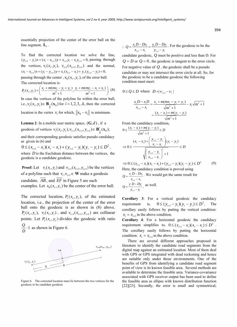
candidate. AB , and EF in Figure 5 are such examples. Let 0( , )r rx x y be the center of the error ball. The corrected location, ( , ),c c cP x y of the estimated location, i.e., the projection of the center of the error ball onto the geodesic is as shown in (8) above.

( , ),c c cP x y ( , )i i iv x y , and 1 1 1( , )i i iv x y are collinear

points. Let ( , )c c cP x y divides the geodesic with ratio

:1Q

D as shown in Figure 6.

Figure 6. The corrected location must lie between the two vertices for the geodesic to be candidate geodesic

1 1

c i c i

i i i i

x D Dx y D DyQ

x x y y

. For the geodesic to be the

candidate geodesic, Q must be positive and less than D. For

Q D or 0Q , the geodesic is tangent to the error circle.

For negative value of Q , the geodesic shall be a pseudo

candidate or may not intersect the error circle at all. So, for the geodesic to be a candidate geodesic the following condition must meet:

0 Q D where

1| |i iD

2

21

( )1

1c i r i i r

ii i

x D x D x m mx y yx m

x x m

2

( ) ( )

1r i r ix x m y y

m

From the candidacy condition,

2

( ) ( )0

1r i r ix x m y y

Dm

1

2

1

1

( ) ( )

0

1

i ir i r i

r i

i i

i i

y yx x y y

x xD

y yx x

21 10 ( )( ) ( )( )i i r i i i r ix x x x y y y y D (9)

Here, the candidacy condition is proved using

1

c i

i i

x D DxQ

x x

. We would get the same result for

1

,c i

i i

y D DyQ

y y

as well.

Corollary 3: For a vertical geodesic the candidacy requirement is, 2

10 ( )( ) .i i r iy y y y D The

corollary easily follows by putting the vertical condition:

1i ix x in the above condition. Corollary 4: For a horizontal geodesic the candidacy requirement simplifies to, 2

10 ( )( )i i r ix x x x D .

The corollary easily follows by putting the horizontal condition: 1i ix x in the above condition.

There are several different approaches proposed in literature to identify the candidate road segments from the digital map against an estimated location. Most of them deal with GPS or GPS integrated with dead reckoning and hence are suitable only under those environments. One of the benefits of GPS from identifying a candidate road segment point of view is its known feasible area. Several methods are available to determine the feasible area. Variance-covariance associated with GPS receiver output has been used to define the feasible area as ellipse with known distribution function [22][23]. Secondly, the error is small and symmetrical;

395


therefore inherently it is less complex to identify the candidate road segments as compared to mobile network. Segment based methods where the heading of the vehicle from GPS points is compared with the road segments in the digital map for maximum parallelism. The road segments that are along the same direction as the line joining the GPS points are marked as the candidate road segments. This method has been used along with other measures [24][25] and as such [26]. Because of the small error and error symmetry this measure is considered quite reliable. However this is not suitable for mobile network, where the error is relatively large and not symmetrical. For example consider Figure 7. A vehicle moves from estimated location L1 to L2 in a mobile network. Clearly segment s2 is the candidate road segment because s2 passes through both the location feasible areas, however using direction similarity, road segment s1 is picked wrongfully. Other disadvantage of this method in mobile system is that we need to have two locations polled very close to one another to identify the candidate road segments.

Figure 7. Vehicle heading from L1 to L2 wrongfully matches the road segment s1

[27] identifies the candidate segment from projection of

the estimated location on to the road segments in the digital map. Let S and E be the two vertices (also referred to as

shaping points) of a geodesic and G be the estimated location point. Define

2

.cos .SG SG SEK

SE SE

(10)

If 0 1K , road segment SE (Figure 8) is selected, if 0K , the road segment preceding the node S is selected, if 1K the road segment following the node E is selected.

The drawback with this method is that it does not take into account the error region. Let us consider a comparison in Figure 8.

It presents two scenarios. In scenario 1, the selected road segment is a valid one, whereas in scenario 2, the selected road segment is not a valid candidate segment contrary to the proposed condition. The candidate selected in scenario 2 is definitely related to some other error circle, since SE does not even touch the error circle. Using this method erroneous

geodesic shall be identified as candidates. This method is only valid for identifying a candidate road segment among the road segments that are fully or partially contained within the GPS feasible area.

Figure 8. In both the projection scenario SE is selected as the candidate segment

[28] identifies the above mentioned flaw in general in finding the candidate geodesic when the vertices of geodesic (or arc in GPS literature) are outside the feasible are. It proposes this problem as future research to address such issue. [12] proposes a method that is along the line of proposed research.

Figure 9.

1 2VV is a candidate geodesic in an error circle of radius r

centered at (h,k)

The proposed conditions to identify a candidate geodesic are as follow: First find the solution ( , ) for the equation of the error

circle, 2 2 2( ) ( )x h y k r and the straight line 1 2VV ,

Figure 9. Here,

2 22

1 2 2 2( , ) ,

1 1

r gm k h mc

m m

(11)

2 22

1 2 2 2( , ) ,

1 1

m r gm k mh c

m m

(12)

where, ,y

mx

, 1 2 1 2x y y xc

x

and

2

( )

1

k mh cg

m

The conditions for candidacy are run online between polls. The calculations must be fast with as little run time as possible. Secondly, depending upon the size of the digital map and the search method, there could be very large

396


number of comparisons and processing required before the next poll. The author proposed for further research to identify candidate segments without solving (11) and (12). Our method identifies candidate geodesics without going through the process of finding ( , ) therefore cutting

significant processing. Secondly, the conditions do not specify which particular solution point,

1 1( , ) or 2 2( , )

to be used for verification. The results would be different for different solution points. This is extremely important from implementation point of view.

C. Discrete Error Balls

The simplest way to form a trajectory is by interpolating the location points collected between the start point and the destination. If we have frequent locations with very low error, hence a large number of points to interpolate, we may potentially come up with a trajectory close to the actual path. However this paper is on forming a trajectory with optimal number of points. As a matter of fact, our trajectory stems from sequence of discrete error balls. How far apart and frequent the error balls are, corresponds to the polling frequency. This is the frequency with which the mobile user’s location is estimated in terms of error ball. The center of the error ball is the estimated location. The polling frequency is directly related to the topology and geometry of the road network the mobile user is traveling on. If a road network is dense and there are numerous intersections, we would need more embedding error balls to estimate the trajectory of a mobile user. On the other hand if roads are sparse with less intersection, for example rural areas, we need fewer error balls to form a trajectory. Let an error ball be located at iC at time i . The next

location of the error ball, 1iC , will be estimated at

time, 1i , using a method, we called it Intersection Polling

Method (IPM). Let ( ) { : ( , ) }i iE

C X d C E B x x

be the

error ball located at ( , )i r rC x y , at i . Let ( , )i i iv x y and

1 1 1( , )i i iv x y be two points on a candidate geodesic of the

error ball. The corrected location on the geodesic as mentioned above, in (8) is

2 2

( ) ( )( , ) , .

1 1r i i r i r i r

c c c

x m mx y y y m my x xP x y

m m

For example in Figure 10, the corrected locations on the

candidate geodesics are 1cP and 2cP . Let 1,i iI I be the

nearest intersections of the road which the geodesic is part of, and si be posted speed of the road segment. The next

position of the error ball is estimated at

1

, 1

1min ,i c k

k i ii

d P Is

, (13)

where d is the metric distance of the Mobile space.

In scenarios where we have multiple candidate geodesics, as shown in Figure 10, the next position of the error ball is estimated at

1 1 2, 1 , 1

1 1min min , , min ,i c k c kk i i k j j

i j

d P I d P Is s

, (14)

where is and js are posted speeds on road segments, iL and

Figure 10. The next position of the error ball is estimated at the nearest intersection from the corrected locations.

,jL respectively. If the roads segments are directional (one-

way) then the candidate intersections are limited to the ones that are towards the directions of the road. In Figure 10 if

the road segments are, 1i iI I

, and 1j jI I

, the candidate

intersection are 1,i jI I . In case there is only one

geodesic passing through the error circle, the direction of motion and hence the candidate intersection assumed is towards the opposite end of the geodesic from the corrected points. It will help in eliminating the intersection that has been a candidate in previous estimation. Let us consider the segment, iL .The probability of the

mobile user is the same on all points of AB . For the estimation of 1i towards iI , if 1cP is taken as the start

point for the estimation of 1i but the mobile user is closer

to point A , the time, 1 ,i would be longer than the

required one. To fix this problem we need to further refine our approach of intersection polling method. In the refined approach instead of assuming the present location of the mobile user, i.e., the location of mobile user at i , we

assume that the present location is the intersection of the geodesic and the error circle. We call this intersection point shifted projection point. Since there are two such shifted projection points, for example A,B for geodesic iL and C,D

for geodesic jL in the figure above, we choose the shifted

projection point that is closer to the road intersection. The shifted projection points of the geodesic, iG with the error

circle ( ) { : ( , ) }i iE

C X d C E C x x

are

1 2( ) G , .i iE

C w wC (14)

397


Where, 2

2 2

1 2 2

22 22

2 2

[( ) / 1 ],

1 1

[( ) / 1 ],

1 1

r rr r

r rr r

E y mx b mmy x mbw

m m

m E y mx b mm y mx b

m m

(15)

2

2 2

2 2 2

22 22

2 2

[( ) / 1 ],

1 1

[( ) / 1 ],

1 1

r rr r

r rr r

E y mx b mmy x mbw

m m

m E y mx b mm y mx b

m m

(16)

The refined IPM dictates that, the location is updated at

1 , 1

1min , .i i ik i i

i

d w Is

We pick iw for which ( , )i id w I is

minimum. Let us briefly analyze the performance of Intersection Polling method in terms of number of polls. The performance of the polling method is directly tied to the topology of the map. Topological factors that directly affect the performance of this method are: the number of intersections during the course of a path and direction of the roads. This polling method would perform the best on longs directional (one-way) roads or the on the grid-like roads, directional or non-directional. Grid-like roads are directional in general anyway. Assuming the start and destination points are arbitrarily anywhere on the roads but not on the intersection, the number of polls required for a path containing N intersections for a grid-like road network are

1N . The advantage comes from the fact that after only one polling the next intersection is identified because the next three intersections are approximately same distance away. Figure 11 depicts part of two-way grid-like road network. The next intersection from L is either A, B or C. Since A, B and C are almost equidistance from L, the polling time for each of them is the same. At the next polling time, any of the intersections, A, B or C, which is contained in the error ball, is map-matched as the next intersection of the path. Therefore for each intersection in the trajectory, only one location polling is enough.

Figure 11. Selection of next intersection in a grid-like road network.

On directional roads of arbitrary layout, the highest number of polls for a path is 2 1N . In this scenario going from one intersection to the other, would require two polls, one for the nearer intersection, the second one for the remaining intersection, i.e., the farther one. Please see Figure 12. Going from the present intersection L, to B, we need to poll

once at *A after time 1, required to reach intersection A

and second poll at B. The number of polls could be reduced to 1N with a minor modification. The modification is;

after polling for the nearer intersection, A, after time 1 ,

pick the other intersection after time 2 1 without

polling, where 2 is the travel time from L to B. The

drawback of this approach is that the destination would always be an intersection. To continue with performance analyses, we stick with our original approach. The lowest number of polls in this scenario is 1N . Here, at each polling the nearer intersection is map matched, for example intersection A, in Figure 12. So, the average number of polls on directional roads with arbitrary layout

Figure 12. Selection of next intersection in a directional road network.

is 31

2N . For non-directional with arbitrary layout road

network, going from one intersection to the next one, we would require maximum three polls. One poll for the nearest intersection, the second one for the nearer of the remaining two intersections and the third one for the last intersection. This scenario is depicted in Figure 13. Here,

LA LB LC . Selection of intersection C is the worst case scenario. Intersection A will be polled first, then B and C respectively. So, we have to poll three times between each intersection in this scenario. So, total number of highest possible polls for a non-directional arbitrary layout of road network is 3 1N . The lowest number of polls on a path on this network would be 1N , as already explained in previous scenarios. Therefore the average number of polls for a path on such road network would be 2 1N . Since GPS location estimation does not cost any additional air resources, estimating the course of trajectory with least number of GPS location points has not been an area of interest. Furthermore most of the vehicles equipped

398


with GPS have DR (Dead Reckoning) integrated also. DR keeps tracks of the length and absolute heading of the displacement vector from previous known position. So, the present estimated location of the vehicle is known at almost all the times. Estimating the trajectory of a vehicle with numerous closely packed location points which have low symmetrical error is far easier than with those which are sparse with relatively larger error especially in urban areas. Let us define an absolute ideal polling method that requires the least number of polling yet does not miss any turns. Most of the proposed methods in GPS world are arc-based (segment based). Such an ideal method would need at least one location point for a directional arc and two location points for a non-directional arc. We assume that this polling method is robust and can handle all the possible topologies of the digital map. An arc is defined as the road segments between two intersections. So, we can estimate the

Figure 13. Selection of next intersection in a two-way road network.

performance of such an ideal polling method in terms of

number of polls. This ideal poller would require 31

2N

polls for an arbitrary path. Let us compare the average performance of Intersection Polling method with this ideal poller. The mean of number of polls required for an arbitrary path in all the three scenarios mentioned above is:

31 1 2 1

32 13 2

N N NN

, which is equal to

the number of polls of an ideal poller using arc-based map matching methods as defined above.

D. Error Ball’s Directional Oreintation

In this section we introduce the notion of error ball’s image. An image of an error ball is, simply, an instance of its previous embedding. The trajectory of a mobile user is essentially estimated from the interpolation of several images of the embedded error ball. So, at a given point during the trajectory formation we have an embedded error ball and several of its images as shown in Figure 14. In the

beginning, obviously, we just have the embedded ball, images are yet to be imprinted. Angle is one of the most important metric for comparing direction. We are interested in comparing the directional orientation of the transition of the error ball with respect to the actual path segments. We call this angle, direction difference. This direction difference is inscribed between the line joining the center of the embedded error circle and its image and a geodesic. In case there are multiple geodesics in the polyline and we are interested in finding the direction difference of this particular path segment and the transition of error ball, we connect the start point (vertex) to the end point of the path segment. The angle it makes with the reference, x-axis we call it the actual direction of motion during that interval.

Figure 14. A graphical representation of our GIS database, error ball and its images.

Since the center of error ball, 1C , and that of its image, 0C

(Figure 15), are not the actual locations of a mobile user at time 1i and i , respectively, the direction difference will

not be accurate. There is an offset in the direction difference.

Figure 15. Illustration of direction of transition of an error ball, , the

direction difference off set, ,and difference error, .

399


In the figure above 1( )E

CB is an error ball centered at 1C

and 0( )E

CB is its previous image with center at 0C . Let

1( )iE

P CB and 0( )iE

Q CB be the two actual locations

of the mobile user, 0 1, i iC C Q P is the direction

error. We define the maximum offset error of an error ball as,

1 0

0 1( ) ( )

max max ,E E

i jj C i C

C C Q P

B B

. (17)

As illustrated in the figure above the maximum offset error is transcribed by the extreme points on the diameters of the two circles, which are diagonally opposite. For example C,B and A,D are such extreme points. Therefore the maximum offset,

1 2tan

E

d

. (18)

Please note is symmetrical, i.e.,

0 1 0 1, , ,C C BC C C AD and it can be easily seen

that 2 2

.

E. Direction Negativity

Let 1 1 1: ,p q be a path segment with start point 1p and end

point 1q and 2 2 2: ,p q be another path segment with start

and end points 2p and 2q , the angle between the two path

1 2 1 1 2 2( , ) ,p q p q is called the direction

difference between paths 1 and 2. A direction negativity

exists between two paths 1 , 2 if 1 2( , )2 2

.

Please note the range of 1 2( , ) is [0, ] or [0, ] .

The maximum negativity is reached when;

1 2( , ) or

This can be clearly visualized if you think one of the paths along the y-axis, i.e., a vertical path, the other path along the positive or the negative side of the x-axis. On either sides of the second path does not contain any y-component in their path. If the direction remains within first quadrant for the positive side of the path and remains within second quadrant for the negative side of the second path, they both have y-components that are positive. If the second path that is along the positive side of the x-axis moves towards fourth quadrant and the one along the negative side of the x-axis

move towards the third quadrant, we start getting the negative y-components in the paths, i.e., they move into direction negativity. If we need to find the angle between a

path, , and the transition of the error ball, 1, ( )E

C B

,

we need to add the offset to 0 1,C C . In a worst case

scenario the offset is, 1 2tan .

E

d

11 0 1

2max , ( ) , tan .

E

EC C C

d

B

(19)

where, d is the displacement of the transition of the error ball. The condition for direction negativity between a path, ,

and transition of the error ball can be easily formulized using inner product. The condition is

1 0 1 01

2 2 2 21 0 1 0

( )( ) ( )( )cos ,

2 2( ) ( ) ( ) ( )

j i j i

j i j i

x x x x y y y y

x x y y x x y y

(20)

where ( , )i ix y and ( , )j jx y are the end points of the path

(or geodesic), , and 1 1( , )x y , 0 0( , )x y are the coordinates

of the center of the error ball and the error ball image,

respectively. Here 2

is taken clockwise which is 3

2

counter clockwise. Please note a proper offset needs to be applied for accurate direction difference.

F. Path Constraint

The different paths between the corrected points in error ball and its previous image are extremely important entity in determining the trajectory of a mobile user. This set of paths is essentially the domain of the possible paths. There are numerous possible paths to connect a projected location from the error ball image to the error ball. We need to assert a constraint to limit the number of paths between the corrected locations. The simplest, yet very pivotal constraint is the travel time. If the travel time of a path between the farthest corrected points is very large than the transition time of the ball, that path is very unlikely. This is very much related to the topology and geometry of the map. In most cases if the travel time of a path is more than twice the transition time of the error ball that path could be eliminated. On directional road, Manhattan style for example, the longest path is five times the direct distance assuming roads around the blocks make a square. The exact time multiplier very much depends on the map topology.

IV. PROSPOSED METHOD FOR TRAJECTORY ESTIMATION

Location Points Collection: Suppose a mobile user starts from home at location A, travels to location B, C, and D,

400


and then comes home at location A. Figure 16 depicts logical parts of this travel trajectory. The points B, C, and D are the rest points. These rest points partition the trajectory into trajectory legs during the whole day of mobility. In this example there are four trajectory legs.

Figure 16. Logical partition of trajectory

We shall describe the mobility profiling method for one leg. For rest of the legs the steps are the same. Step 1: Poll the mobile user for his location. Find the candidate geodesics as described in Section III B. Step 2: Repeat Step 1 after determining polling time as described in Sections III C. Continue polling until destination of the leg is reached. Step 3: Apply the condition for directional negativity to eliminate multiple geodesics in the error ball as explained in Section III E, please see Figure 17. Step 4: Apply the path constrains using appropriate time multiplier as explained in Section III F. Step 5: Map match the so obtained curve or set of curves with the digital map to obtain the closest to shape trajectory of the travel leg. Please see Figure 19.

Figure 17. Direction negativity and path constrains on error ball and its images. If the user was on University Ave E prior to the recent last two

polls shown in this picture, after applying the constraints, we are left with t only two candidates roads which are shown in broken blue lines.

Figure 18. Trajectory estimation flow chart.

Figure 19. Map matching of pre-matched candidate curve with the set from GIS database.

401


A flow chart of the detailed algorithm is shown in Figure 18. The algorithm was implemented using C# (C sharp) in Microsoft windows. C# fulfilled the graphics requirements we needed for our simulation easily.

V. IMPLEMENTATION OF PROPOSED METHOD

The implementation has two parts, as described in the following subsections.

A. GIS Database of Road Networks

Our mobility profiling system is essentially a GIS embedded with a cellular system. The cellular part of the system estimates the mobile location; the GIS part corrects the estimated location and provides all necessary references for trajectory estimation. Database is the backbone of a GIS. For trajectory estimation we use a digital database of a road network. We have paper road maps, Figures 21 (scale 1:10,000) and 22 (scale 1:50,000), which need to be digitized to make a digital database. We use vector format data of a road network. Manual digitization is one of the widely used methods to digitize a paper map to vector data. It uses a digitizing table. A digitizing table is essentially an input device that interfaces with a computer, to store the coded data in the form of coordinate points. A digitizing table is an expensive tool. We developed a Microsoft Windows based application that emulates a digitizing table. The digitizing application, let us call it Digitizer from this point on, is not hard coded to exclusively digitize the maps shown in Figures 21, and 22 but it can load any map that needs to be digitized using the user interfaces depicted in Figure 20. The whole digitization process is a little labor intensive. We used point mode digitization .

Figure 20. Digitizer’s GUI.

The map image could be in JIFF, BMP, or JPEG format. Once the image is loaded the digitization starts by naming the road segment, i.e., polyline, and selecting the posted speed, and direction attribute of the road segment. The segments are digitized by mouse clicks at important points using point mode method. The most effective feature in the Digitizer is zooming, Figure. 21. This is where the Digitizer adds value in accuracy. The main source in digitization error is introduced by the operator who is doing the digitization [29][30]. One of the main reasons of operator’s error in digitizing roads is that some roads are not thick enough on the map and it is difficult to stay on the center line of the road. The operator is supposed to stay within a band centered on the road center line. In cartography it is referred as epsilon band [31]. Zoom feature will help the operator to

stay within the epsilon band and closer to the center line. The zoom window features a very fine pointer for further

Figure 21. Zoom feature of the Digitizer helps in digitization by hand. The map being digitized is of an urban area of Saint Paul Minnesota.

accuracy. On thin or closely packed roads as shown in zoom window, the accuracy is about four times that that of a digitizing table. Since an operator concentrates on only one screen as compared to the digitizing table where the operator’s attention is divided into two places, the monitor screen and the map, digitizing with software version of the digitizing table is more efficient. Once a map is digitized using a digitizing table, its digitized version is verified with zoom feature on the computer. So, zoom is a reliable feature in cartography world already. The process of manual digitization is a psychophysical process that depends on a harmony between human perception, adjustment of mental impression and physical balance of arm muscles [32], so, the accuracy of manual digitations varies from operator to operator. Manual digitization error on a 1:24,000 map ranges from 20-55 feet. Using a feature like zoom would reduce the error significantly.

The intersecting roads have a common point which must be selected as one of the points of the road segments during their digitization. One issue while marking this common point is that, one may be few pixels off while marking this point during the definition (digitization) of each road segment. This issue is remedied with one of the features of Digitizer; we called it “Unification Threshold”. To combine points on different road segments into one intersecting point, we right click the mouse around the points, a unifying routine combines all the points in the threshold area. The threshold area is configurable as shown in Figure 20. After all roads are digitized and stored in the database, the ASCII database was converted to binary for faster access. We can convert ASCII data to binary and binary to ASCII. To verify the accuracy of the so obtained digitized database, we reconstructed the road network from the data accurately.

402


The mobility trajectory estimation simulation was done in two different topological scenarios: an urban area of St. Paul, Minnesota and suburban area of North Carolina. We digitized two maps, one shown in Figure 21 (urban) and the other one depicted in Figure 22 (suburban).

Figure 22. Map of suburban area digitized for GIS database.

The digitized version of the maps mentioned above are given below, Figures 23 and 24. Please note these maps are erected from the GIS data base as mentioned in Section II B.

Figure 23. Reconstruction of map of Figure 21 from GIS database.

Figure 24. Reconstruction of map of Figure 22 from GIS database.

B. Mobility Profile Simulation

To simulate, the mobile user’s mobility, we developed another Windows based application, Mobility Profiler Simulator. The application has two major parts: one simulates mobility of the mobile user via traversing of a dinky car on the road network of a map; the other is an implementation of the mobility profiling method described in section IV. Figure 25 depicts the mobility simulation window of the application.

An optional step after invoking the application is to load the reference map image for viewing the simulation with respect to the map. Then digital map (GIS database) is loaded into the application. This is the actual road network which is referenced by the mobility profiler for location polling and map matching. The dinky car traverses on the path provided by the so called “path file”. The path file is a text file containing the points and line segment information that defines a particular path for the mobile user. After path is loaded, the simulation is started from another window. The dinky car, shown in the circle in Figure 25, travels along the paths dictated in the path profile. This simulates the actual mobility of the mobile user. The Mobility Profiler Simulator estimates the mobile trajectory independently by polling mobile user’s locations, correcting them by identifying the road segments and them combining the road segments.

The animation speed of the dinky car can be increased or decreased for demonstration purposes using the control option called Animation Speed. The dinky car travels on the

403


Figure 25. Mobility Profiling simulator’s GUI, the mobility simulation window.

road segments according to the posted speed on them. A variation on the speed can be adjusted. The polling agent in mobility profiler polls for location of the car according to an implementation of Intersection Polling method, described in details in Section III C. The location is estimated with a random error. The process of location polling has been animated in the application to depict how it would happen in the actual deployment in the field.. In this process the polling agent inquires the exact location of the dinky car, the location is returned to the profiler with a radiating signal (animation) from the car, adding a random error. The error has been modeled with a circle of radius equal to the error associated with the underlying location estimation technology and centered at the returned estimated location.

The second window of the application, the mobility profiler, is invoked from a menu from the first application. This part of the simulator provides the interface for input variables; the location estimation error of the underlying location estimation technology and the posted speed variations. We can define lower and upper bounds for the speed variation in the posted speed of GIS database. These input variables are entered in the counters shown in red rectangles in the Figure 26. This window plots the trajectory per algorithm given in flow chart in Figure 18. During the first parsing of the simulation candidate road segments and the corresponding location points are determined. In the second parsing, direction and the distance constraints are applied. After these constraints are applied, the estimated trajectory is plotted as show in Figure 26.

If this trajectory does not match exactly with a trajectory from the digital map, we map match it with our digital map. In most of the cases the constraints rectify the shape of the trajectory. The actual path (from path file) and the estimated trajectory, both, are plotted in the simulator window. The reference map, which merely acts as background image makes the simulation result more meaningful for viewing, Figure 27. This gives a better understanding of the error in

Figure 26. Mobility profiling simulator’s GUI, the trajectory estimation window.

the estimated trajectory. It shows the exact locations on the map where the estimated trajectory deviates from the actual one. The option Offset XY translates the reference trajectory right and down according to the set values in these counters for easy viewing and comparing of the two trajectories. Please refer to the first rectangle in the menu bar in Figure 26.

Figure 27. Mobility profiling simulator window with reference map.

404


All the simulation results are presented with reference path and reference map as shown in Figure 27. The green curve (darker if black and white) depicts the actual path whereas the blue curve (lighter if black and white) is the estimated trajectory. We ran the simulation, both in urban and suburban areas. The main variables in the simulation are the location error and the speed variation, which we could vary during the simulation also, if needed. After a simulation finishes, the mobility profiler prints important statistics pertaining to the simulation. It prints the following statistics:

Percentage of segments identified correctly Average Along Track Error Average Cross Track Error Average Error along X-axis Average Error along Y-axis Total number of location polls Linear Error ( defined in next section) Areal Error (defined in next section)

VI. TRAJECTORY ESTIMATION SIMULATION

Location points are building blocks of a trajectory. The estimated location of a mobile user does not necessarily map on a road because of the error in location estimation methods. Among the vertices defining roads, the points corresponding to roads intersections play a pivotal role. In urban area the roads are densely populated hence a large number of road intersections. This results in potentially high number of turns that leads to high polling frequency. Secondly, because of high road density, an error area (estimated location) encloses a large number of roads. On the other hand in rural or suburban areas the road density is smaller as compared to urban areas; therefore estimated location corresponds to fewer roads as candidates of the mobile user trajectory. So, the rural areas should provide more accurate user’s trajectory. In this chapter we investigate both scenarios and provide the simulation results. We shall demonstrate how estimated location error affects the accuracy of the mobile user’s trajectory. We shall correlate the error with the underlying location estimation technologies and present suitability of the location technology under different road topologies.

Our estimated trajectory is represented as a sequence of points, so essentially as a set. The error associated with the estimated trajectory is a measure of dissimilarity between the actual and estimated trajectories. The actual trajectory is also a sequence of points, so Hausdorff distance [33] would be natural choice as an error index. However the problem with Hausdorff distance is that, it gives the shortest distance between two points in the sets and it does not cover the course of the distance traveled. Therefore using Hausdorff distance to measure the dissimilarity would lead to wrong findings. The issue with Hausdorff distance is covered in Fréchet distance [34]; it takes the course of distance into account. It is explained by man-dog example in literature [35][36]. Fréchet distance is widely used to find distance

(dissimilarity) between two curves. The curves are approximated as polygonal figures as done in the case of roads. However Fréchet distance shows an anomaly when comparing the two trajectories as depicted in Figure 28. The dissimilarity between two paths A and B and that of between A and C, according to Fréchet distance is the same, which is misleading.

Figure 28. Anomaly in Fréchet distance.

The Fréchet distance between A and B is 8, which is also the case with A and C. Clearly A and C are more dissimilar than A and B. Therefore we need to define a meaningful index of error for an estimated trajectory. We called this error Trajectory Estimation Error (TEE). TEE can be represented as linear error or areal error as defined below. Both, linear and areal errors together, give a good understanding of the trajectory estimation error.

A. Linear Error

Linear error demonstrates the length of the actual trajectory that is missing in the estimated trajectory. It is ratio of the path length that is erroneous, e , to the total path length t .

.eL

t

E

(21)

B. Areal Error

Areal error demonstrates the dissimilarity between the two trajectories (curve), the actual and the estimated one by the area bounded by them as shown in Figure 28. According to Fréchet distance the two set of curves, A,B and A,C are equally dissimilar, however their areal error portrays a better error index. For better comparison of areal error, bounded area per unit length of trajectory would be a better index of error. The areal error per unit length is:

.AEL

(22)

Where, is the error area, and L is the total length of the actual trajectory. We have used linear error along with areal error to get a better degree of comparison between actual and the estimated trajectories.

405


C. Trjectory Estimation Simulation Results

Trajectory estimation simulation was performed using two digital maps discussed above, one for urban area of Saint Paul Minnesota and the other for suburban area of North Carolina. A range of error corresponding to different location estimation technologies was used for the simulation. Figures 29 through 38 show the simulation results for an urban area for different location error. Green trajectory is the actual trajectory whereas the blue is the estimated one.

Figure 29. Result with location error of 25m.



In urban area for location error of 50m or less, the trajectory error was on the closely parallel roads only (Figures 29 and 30). However, for larger location error, 100m and more, the trajectory error expanded farther than the closely parallel roads (Figures 32 through 37). Figure 38 shows a graph for location error versus trajectory error for the urban area.


406



For the suburban area the algorithm missed only a short segment of trajectory (Figures 40 through 42), even for large location error of 400m. We get this performance because of low number of intersections per unit area in suburban areas.



Both areal and linear errors in trajectory estimation not only stem from location estimation error, but are intrinsic to the map topology and path. For example, if we choose a different path the same parameters used in Figure 36 would yield a different result, please see Figure 37.


407


Figure 37. En error of 200 m yields higher trajectory error using dense part of the map.

The relationship of Trajectory Estimation Error (TEE) to the location estimation error (LEE) can be easily interpreted from the results above. Figure 38 depicts the LEE-TEE relationship for LEE of 0-200m with a step of 25m. For urban area, after 200m of LEE, the trajectories are not reliable for profiling. TEEs depicted in the graph are the typical values for ten simulations for each LEE. For smaller location estimation errors, 25m and 50m, each simulation run for that particular LEE gave almost similar trajectory. The error mainly comes from the two parallel roads about thirty meters apart. For LEE of 75m and 100m, there was some difference in the shape of trajectory for each run. After around 125m of LEE the trajectory curve (shape) varies significantly for each run with the same LEE, because the error circle was large enough to start inscribing multiple candidate road segments and road intersections. The three rectangles in Figure 38 provide a reference of known accuracy of different location estimation technologies, namely Assisted GPS, TDOA technologies such as E-OTD and U-TDOA (Uplink-TDOA), and AOA. It is evident from the figure which location estimation technologies suit for mobile trajectory estimation. It is important to note that dependence of TEE on LEE is very much tied to the map topology and the trajectory of the mobile user. Within the same map two trajectories of the same length under same LEE would lead to different set of linear and areal error as observed in comparing Figures 36 and 37. Since our

location error is random with the upper bound of ,E

with

each run of LEE for specific ,E

we get different values of

TEE. This is true for both, linear and areal errors. With large number of simulation runs we get a range of TEE related to LEE. As LEE increases the range widens as expected. Please see Figure 39.

Figure 38. Trajectory estimation error vs location estimation error related to different location estimation techniques.

Figure 39. Linear and Areal Error Ranges.

Figures 40 through 42 show simulation results for rural area shown in map in Figure 22 for error of 100m, 200m and 400m respectively. The results are the same for these location error. The mobility profiler missed a small corner near the main highway. For smaller location error around 50 m, this minor error in trajectory estimation dimishes. This

408


behavior is manifested because there are two parallel path that are about 100 m apart and the both of them are candidate road segment. The segment that is picked in estimation is more closer in shape of the curve prescribed by the estimation location points.

Figure 40. Suburban Trajectory estimation with 100m error.


Figure 42. Suburban Trajectory estimation with 400 m error.

VII. CONCLUSION

We applied the proposed trajectory estimation algorithm in two field scenarios; urban area and rural area. The objective was to determine how existing location estimation technologies would perform with the algorithm in urban and suburban areas. In urban area, where road network is dense and consequently there are a large number of potential turns for a mobile user, the trajectory error increases sharply with the error of underlying location estimation technology. Even within the urban area, the topological and geographical differences between different parts of the same road network bring about substantial difference in the accuracy of the estimated trajectory as seen in comparing Figures 36 and 37. The right half of the road network in Figures 36 has fewer turns. There are fewer inlets and outlet points per unit area on that side of the network. That’s why; increasing the location estimation error did not affect that part of the road network as much as it did on the other side. When same location error was applied to a different path going through higher number of potential turns (Figure 37) the error increased to almost double. With the increase of LEE not only TEE increases, but also the number of location polls required estimating the mobile trajectory. Even under topological and geographical constraints, with larger error, it requires a larger number of polls to get out of the cluster of roads. These roads are enclosed within the error circle. Larger the error is, more candidate road segments for trajectory estimation are enclosed in the error circle. So, in urban area relatively precise location estimation methods like A-GPS or accurate time based methods such as EOTD are best suited for trajectory estimation. Whereas in suburban or

409


rural area, almost all technologies that fulfill E-911 mandate [3] qualify to estimate trajectory with good accuracy.

REFERENCES

[1] Sarfraz Khokhar, and Arne A. Nilsson, “Estimation of mobile trajectory in a wireless network: A basis for user’s mobility profiling for mobile trajectoy based services,” 3rd International Conference on Sensor Technologies and Applications, Athens, 2009.

[2] Elliott D. Kaplan, and Christopher Hegarty, “Understanding GPS: Principles and applications,” Artech House Publishers, 2005, Second Edition.

[3] Allison Kealy, Stephan Winter, and Günther Retscher, “Intelligent location models for next generation location-based services,” Journal of Location Based Services, vol. 1, Issue 4, December 2007, pp. 237–255.

[4] Lin Ding-Bing , Juan G Rong-Terng, and Lin Hsin-Piao, “Mobile location estimation and tracking for GSM systems,” Fifteenth IEEE International Symposium on Personal, Indoor, and Mobile Radio Communications , Barcelona , 2004 , pp. 2835–2839.

[5] Sarfraz Khokhar, Arne. A. Nilsson, and Mo-Yuen Chow, “Mobile location estimation methods,” GIS 2001 Conference & Exposition, Vancouver, BC, February, 2001.

[6] Sarfraz khokhar, Arne A. Nilsson, “Introduction to mobile trajectory based services: A new direction in mobile location based services,” International Conference on Wireless Algorithms, Systems and Applications, Boston 2009, Springer-Verlag Berlin Heidelberg, pp. 398–407.

[7] Stanley Sokolowski, Raymond L. Filler, Nhut Vo, and Paul Olson, “Enhanced C2 functionality in urban and other complex terrain,” IEEE Military Communications Conference, vol. 1, 17-20 October, 2005, pp. 258–264.

[8] Goran M. Djuknic, and Robert E. Richton, “Geolocation and assisted GPS,” Computer, Volume 34, Issue 2, February, 2001, pp. 123–125.

[9] Wenjie Liao, Weifeng Lv, Tongyu Zhu, and Dong Dong Wu, “A map matching algorithm for intersections based on Floating Car Data,” 10th International Conference on Advanced Communication Technology, vol. 1, 17-20 February, 2008, pp. 311–316.

[10] David Bernstein, and Alain Kornhauser, “An introduction to map matching for personal navigation assistants, ” New Jersey TIDE Center 1996.

[11] Chenhao Wang, Zhencheng Hu, and Keiichi Uchimura, “A Precise road network modeling and map matching for vehicle navigation,” 11th International IEEE Conference on Intelligent Transportation Systems, 12-15 October, 2008, pp. 1084–1089.

[12] Mohammed A. Quddus, “High integrity map matching algorithms for advanced transport telematics applications,” Centre for Transport Studies, Imperial College London, United Kingdom, January, 2006.

[13] Hong-mei Yin, and Shan-wu Su, “Modeling for geospatial database of national fundamental geographic information,” IEEE International Conference on Geoscience and Remote Sensing, 2006, pp. 865–868.

[14] Stephen Wise, “GIS Basics,” Taylor & Francis, April, 2007.

[15] Dean Pomerleau, “A neural network based autonomous navigation,” Vision and Navigation, Kluwer Academic Publishers, 1990.

[16] Surender K. Kenue, “LAMELOK:Detection of lane boundaries and vehicle tracking using image-processing techniques,” Parts I and II, SPIE Mobile Robots IV, 1989.

[17] E.D. Dickmanns, R. Behringer, D. Dickmanns, T. Hildebrandt, M. Maurer, F. Thomanek, and J. Schiehlen, “The seeing passenger car ‘VaMoRs-P’,” Proceedings of the Intelligent Vehicle Symposium, 1994, pp. 68 –73.

[18] Karl Kluge, and Charles Thorpe, “Representation and recovery of road geometry in YARF,” Proceedings of the Intelligent Vehicles Symposium, 1994, pp. 1141–19.

[19] Mathew A. Turk, David G. Morgenthaler, Keith D. Gremban, and Martin Marra, “VITS: A vision system for autonomous land vehicle navigation,” IEEE Transactions on Pattern Analysis and Machine Intelligence, vol. 10, Issue 3, May, 1988, pp. 342 3–61.

[20] Satish Shirali, and Harkrishan L.Vasudeva, “Metric spaces,” Springer-Verlog London Limited, 2006.

[21] Sulata Mitra, and Sipra DasBit, “On location tracking and load balancing in cellular mobile environment- A probabilistic approach,” 5th International Conference on Electrical and Computer Engineering , December, 2008, Dhaka, Bangladesh.

[22] Washington. Y. Ochieng, Mohammad A. Quddus, and R.B. Noland, "Map-matching in complex urban road networks," RBC - Revista Brasileira de Cartografia, N⁰ 55/2, dezembro, 2003.

[23] Khalid Touil, Mourad Zribi, and Mohammed Benjelloun, “Application of transferable belief model to navigation system, Integrated Computer-Aided Engineering,” IOS Press, 2007, pp. 93–105.

[24] Mohammad A. Quddus, Washington. Y. Ochieng, L. Zhao, and Robert .B. Noland, “A general map matching algorithm for transport telematics applications”, GPS Solutions, 2003, pp.157–167.

[25] Yu Meng, Zhilin Li, Wu Chen, and Yongqi Chen, "Reliability and integrity issues for vehicle positioning systems," The International Symposium on GNSS/GPS, Sydney, Australia, December, 2004.

[26] Sudarshan S. Chawathe, “Segment-based map matching,” Intelligent Vehicles Symposium, June, 2007, pp. 1190–1197.

[27] Pen -Shan Hung , Tsui -Chuan Su, "Map-matching algorithm of gps vehicle navigation system," Geographic Information System Research Center, Reng Chia University, Taichung, Taiwan, 1998.

[28] Mohammed A. Quddus , Washington Y. Ochieng, and Robert B. Noland, "Current map-matching algorithms for transportation applications: State-of-the art and future research directions," Transportation Research Part C, vol. 15, 2007, pp. 312–328.

[29] Paul V. Bolstad, and James L. Smith, “Errors in GIS assessing spatial data accuracy,” Journal of Forestry, November, 1992, pp. 21–29.

[30] Paul V. Bolstand, Paul Gessler, and Thomas M. Lillesand, “Positional uncertainty in manually digitized map data,” International Journal of Geographical Information Systems, vol. 4, 1990, pp.399–412.

[31] R. Dunn, A. R. Harrison, and J. C. White, “Positional accuracy and measurement in digital database of land use: an empirical study,” International Journal of Geographical Information Systems, vol. 4, 1990, pp. 385–398.

[32] M. M. Yagoub, “The effect of psychophysics on the I of GIS/LIS,” Geoinformatics and Socioinformatics, The Proceedings of Geoinformatics Conference, Ann Arbor, 19-21 June, 1999, pp. 1–9.

[33] Helmut Alt, and Ludmila Scharf, “Computing the Hausdorff distance between curved objects,” The 20th European Workshop on Computational Geometry, 2004, pp. 233–236.

410


[34] Günter Rote, “Computing the Fréchet distance between piecewise smooth curves,” The 20th European Workshop on Computational Geometry, 2004, pp. 147–150.

[35] R. Sriraghavendra, K. Karthik, and Chiranjib Bhattacharyya, “Fréchet distance based approach for searching online handwritten documents”, Ninth International Conference on Document Analysis and Recognition , vol. 1, 23-26 September, 2007, pp. 461–465.

[36] Hui Ding, G. Trajcevski, and P. Scheuermann, “Efficient similarity join of large sets of moving object trajectories,” 15th International Symposium on Temporal Representation and Reasoning, 16-18 June, 2008, pp. 79–87.

411


Towards an Optimal Positioning of Multiple Mobile Sinks in WSNs for Buildings

Leila Ben Saad, Bernard TourancheauLIP UMR 5668 of CNRS-ENS Lyon-INRIA-UCB Lyon

Lyon, France{Leila.Ben.Saad, Bernard.Tourancheau}@ens-lyon.fr

Abstract

The need for wireless sensor networks is rapidly growingin a wide range of applications specially for buildingsautomation. In such networks, a large number of sensorswith limited energy supply are in charge of relaying thesensed data hop by hop to the nearest sink. The sensorsclosest to the sinks deplete their energy much faster thandistant nodes because they carry heavy traffic which causesprematurely the end of the network lifetime. Employingmobile sinks can alleviate this problem by distributing thehigh traffic load among the sensors and increase the networklifetime. In this work, we aim to find the best way to relocatesinks inside buildings by determining their optimal locationsand the duration of their sojourn time. Therefore, we proposean Integer Linear Program for multiple mobile sinks whichdirectly maximizes the network lifetime instead of minimizingthe energy consumption or maximizing the residual energy,which is what was done in previous solutions. We evalu-ated the performance of our approach by simulation andcompared it with others schemes. The results show thatour solution extends significantly the network lifetime andbalances notably the energy consumption among the nodes.

Index Terms

Wireless Sensor Networks, Sinks positioning, Mobilesinks, Network lifetime, Integer Linear Programming.

1. Introduction

Recent years have witnessed an increasing need for wire-less sensor networks (WSNs) in a wide range of applicationsspecially for buildings automation. In fact, the WSNs canbe used as a way to reduce the waste of energy insidebuildings by reporting essential information from the in-door environment allowing, for instance, to turn off theunnecessary electric appliances in the rooms. Nevertheless,wireless sensor networks deployment inside buildings is avery challenging problem[1]. Such networks are composedof low cost tiny devices with sensing, data processing andcommunication capabilities. These sensors have a short oper-ational life because they are equipped with a limited number

of batteries supplying energy. Moreover, it is usually imprac-tical and even impossible to replace or recharge them. Thesensors, which are densely deployed in the area of interest,measure and monitor their indoor environment (temperature,humidity, light, sound, etc.,) and collaborate to forward thesemeasurements towards the nearest resource-rich collector,referred to as the sink node. The sensor nodes which arefar away from the sink use multi-hops communication. Thismean of communication makes the sensors near the sinksdeplete their energy much faster than distant nodes becausethey carry the packets of sensors located farther away inaddition to their own packets. Therefore, what is known asa hole appears around the sinks and makes distant nodesunreachable and unable to send their data. Consequently,the network lifetime ends prematurely.

More and more efforts have been done recently to im-prove the lifetime of WSNs. Many communication proto-cols have been proposed including among others topologycontrol[2][3], routing[4][5] and clustering[6]. However, fur-ther improvement can be achieved if we relocate the sinks inorder to change over time the nodes located close to them.Thus, this can solve the energy hole problem and guaranteebalanced energy consumption among the nodes.

In this work, our purpose is to determine where to placemultiple sinks inside buildings, how long they have to stayin certain locations and where to move them to extendoptimally the network lifetime. To answer these questions,we propose an Integer Linear Program (ILP) for multiplemobile sinks whose objective function directly maximizesthe network lifetime instead of minimizing the energy con-sumption or maximizing the residual energy, which is whatwas done in previous solutions[7][8].

The contribution of our work concerns not only the defi-nition of an ILP which determines the optimal locations ofmultiple mobile sinks but also shows that relocating mobilesinks inside a whole network is more efficient than relocatingmobile sinks inside different clusters. Simulation resultsshow that with our proposed solution, the network lifetimeis extended and the energy consumption is more balancedamong the nodes. Moreover, the lifetime improvement thatcan be achieved when relocating 3 sinks in a network withhundred sensors is almost 230 % in our experiments. Suchresults can provide useful guidelines for real wireless sensornetwork deployment.

412


The rest of this paper is organized as follows. In Section2, we review the previously proposed approaches to solvethe energy hole problem and extend the network lifetime inWSNs. Section 3 describes the system model including themajor assumptions. Section 4 presents the formulation of ourproposed ILP for multiple mobile sinks. Section 5 evaluatesthe performance of the proposed solution and presents theexperimental results. Section 6 concludes the paper.

2. Related Work

In order to improve the network lifetime of WSNs, manyresearchers looked for approaches that help to solve theenergy hole problem. Several solutions proposed to placemore sensor nodes around the sink[9][10][11]. This solutionis called nonuniform node distribution and consists in addingnodes to the areas with heavier traffic in order to createdifferent node densities. However, these solutions are notalways feasible in practice and result in unbalanced sensingcoverage over different regions of the network.

Another way of optimizing the network lifetime is to usemultiple sinks instead of one in order to decrease the averageof packets that has to pass through the nodes close to thesinks. The location of these sinks has a great influence onthe network lifetime. For this reason, many works focusedon the optimal placement of multiple static sinks in WSNs.The majority of the sinks placement problem formulationsare NP-complete depending on the assumptions and networkmodel. Therefore to reduce this complexity, approximationalgorithms were used[12] and heuristics were adopted toreduce the energy dissipation at each node[13]. In [14], theproblem was formulated by a linear programming model tofind the optimal positions of static sinks and the optimaltraffic flow rate of routing paths in WSNs.

Most of the optimal multi-sinks positioning approachesdescribed previously contribute to increase the networklifetime. Nevertheless, it was proved in [15] that using amobile sink is more efficient than a static one and achievesfurther improvements in network lifetime by distributing theload of the nodes close to the sink. Furthermore, the sinkmobility has many other advantages. In fact, it can improvethe connectivity of the isolated sensors and may guaranteethe sink security in case of malicious attacks.

The majority of related works studied the mobility ofa single sink[15][16][17][18][19][20]. But, very few re-searches focused on the mobility of multiple sinks. In [17],the solution of repositioning a single sink is extended toa network with several sinks by dividing it into severalclusters. Each sink can only move in its cluster.

There are basically three categories of sink mobility.Mobile sink may move in a fixed path[15], may take arandom path[21] or may move in optimal locations in termsof network lifetime and energy consumption.

The authors of the paper [15] suggested that the sinkmoves on the periphery of the network to gather the dataof the sensors deployed within a circle. The authors of [21]proposed to use ”Data Mules” which move randomly on thesensor field and collect data from the nodes.

An often used way to determine the locations of mobilesinks in the third category is to develop an algorithm.Some proposed algorithms make a moving decision ofsinks according to the complete knowledge of the energydistribution of the sensors. In [22], the sinks move towardsthe nodes that have the highest residual energy. But, thisstrategy requires that the sensors send periodically to the sinkadditional information about their energy level to allow thesink to found out the nodes which have the highest energy.By doing so, a lot of energy will be wasted.

Some others algorithms find the locations of mobilesinks by solving a mathematical model[23][24]. In [23], thealgorithm minimizes the average distances between sensorsand nearest sinks. In [24], the algorithm selects the locationsof sinks in the periphery of the network in such way that thedifference between the maximum and the minimum residualenergy of nodes is minimized.

To find the optimal locations of mobile sinks, some pro-posals formulated the problem as an Integer Linear ProgramILP. In [8], the proposed ILP maximizes the minimumresidual energy over all nodes. In [7], the proposed ILPminimizes the energy consumed at each node.

Most of proposed approaches to determine the locationsof multiple mobile sinks in WSNs are centered on energyminimization. In our work, a different formulation of theproblem is proposed, where the ILP proposed directly max-imizes the network lifetime instead of minimizing the energyconsumption or maximizing the residual energy. To us, thisis closer to the need of sensors deployment in buildingmonitoring for instance.

3. System Model

In order to deploy sensors and sinks inside buildings, wemade the following assumptions for the system model.

3.1. Network Model

- All sensors are statically placed in a bi-dimensional gridof same size cells constructed from the building planas shown in Figure 1.

- All sensors have a limited initial energy supply and afixed transmission range equal to the distance betweentwo nodes (i.e, cell size).

- Each sensor regularly generates the same amount ofdata.

- The number of sinks is fixed and known beforehand.- The sinks can be located only in feasible sites where

they are connected to power supply and the Internet.

413


Figure 1. 10x10 Grid of cells with 100 sensors

- The sinks keep moving in the grid from one feasiblesite to another one until the network lifetime end.

- The network lifetime is defined as the time until thefirst sensor dies (i.e, it uses up its residual energy).

- The sinks should stay at a feasible site for at least acertain duration of time. At the end of this duration,they may stay or change of location.

- The traveling time of sinks between feasible sites isconsidered negligible for analytical simplicity.

- The sensor nodes which are not co-located with anysinks inside the grid, relay their generated data viamultiple hops to reach the nearest sink.

- An ideal MAC layer with no collisions and retransmis-sions is assumed.

- In our assumptions, only the energy consumption forcommunication is considered due to the fact that com-munication is the dominant power consumer in a sensornode.

3.2. Routing and Path Selection

The sensor nodes which are not co-located with any sinksinside the grid send their generated data hop by hop to thenearest sink. When a sensor node is located in the samehorizontal or vertical line of the nearest sink position, thereis only one shortest path between the two nodes. Otherwise,there are multiple shortest paths. In our routing protocol likein [18], we route ”per dimension”. We consider only the twopaths along the perimeter of the rectangle, i.e., paths 1 and2 in Figure 2. These two routes are considered equivalent.

3.3. Power Consumption

To calculate the power consumption, we consider the samerealistic model as in [25]. Therefore, the power expended totransmit a L1-bit/s to a distance d is:

PTx = L1γ1 + L1γ2dβ (1)

Figure 2. Path selection

where γ1 is the energy consumption factor indicating thepower consumed per bit by the sensor to activate transceivercircuitry, γ2 is the energy consumption factor indicating thepower consumed per bit by the transmit amplifier to achievean acceptable energy per bit over noise spectral density andβ is the path loss exponent. The power expended to receiveL2-bit/s in the same radio model is:

PRx= L2α (2)

where α is the energy consumption factor indicating thepower consumed per bit at receiver circuit. Thus, the totalenergy consumed by a sensor node per time unit is:

Ptotal = PTx + PRx = L1(γ1 + γ2dβ) + L2α (3)

4. Integer Linear Programming Formulation

The WSN is represented by the graph G(V, E), whereV = S ∪ F and E ⊆ V × V . S represents the set ofsensors nodes, F represents the set of feasible sites andE represents the set of wireless links. We distinguish twoscenarios with mobile sinks. The first one is when there aremultiple sinks moving in the entire network. The second oneis when there are multiple sinks moving separately insidedifferent clusters.

4.1. Mobile sinks moving in the entire network

The parameters and variables used to describe theproblem are the following:

• Parameters- m is the number of sinks.- T (s) is the minimum duration of common time

units for which the sink should stay at a certainfeasible site.

- e0 (J) is the initial energy of each sensor.- eT (J/bit) is the energy consumption coefficient for

transmitting one bit.- eR (J/bit) is the energy consumption coefficient for

receiving one bit.- gr (bit/s) is the rate at which data packets are

generated.

414


- rkij (bit/s) is the data transmission rate from node

i to node j where the nearest sink stays at node k.- Nk

i is the set of i’s neighbors whose their nearestsink is at node k.

- pk1k2...km

i (J/s) is the power consumed in sendingand receiving data by sensor node i when thefirst sink is located at node k1, the second sink islocated at node k2 etc. and the m-th sink is locatedat node km.

- pki (J/s) is the power consumed in sending and

receiving data by sensor node i when the nearestsink is located at node k, k ∈ F .

• Variables- Z (s) is the network lifetime.- l

k1k2...kmis an integer variable which represents

the number of times when the first sink is locatedat node k1, the second sink is located at node k2

etc. and the m-th sink is located at node km fora duration of time T , k1 ∈ F , k2 ∈ F and km ∈ F .

max Z =∑

k1∈F

∑

k2∈F

...∑

km∈F

T lk1k2...km

(4)

∑

k1∈F

∑

k2∈F

...∑

km∈F

T lk1k2...km

pk1k2...km

i ≤ e0, i ∈ S (5)

lk1k2...km

≥ 0, k1 ∈ F, k2 ∈ F, ..., km ∈ F (6)

The equation (4) maximizes the network lifetime anddetermines the sojourn times of all sinks at feasible sites. Theequation (5) assures that the energy consumed in receivingand transmitting data by each sensor node doesn’t exceed itsinitial energy. This energy is computed when the first sinkis located at node k1, the second sink is located at node k2

etc. and the m-th sink is located at node km.The power pk1k2...km

i is computed as following:

pk1k2...km

i = pki (7)

where k=NearestSink(k1, k2, ..., km, i), NearestSink isa function which returns the nearest sink node to sensor nodei. This sink node is determined by choosing the shortest pathas presented in Section 3.2.

In our model, the energy consumption coefficient fortransmitting a bit denoted by eT and the energy consumptioncoefficient for receiving a bit denoted by eR are constant:

eT = γ1 + γ2dβ (8)

eR = α (9)

From the equation (3), the total power consumed at asensor node is:

Ptotal = eT L1 + eRL2 (10)

Therefore, the pki is calculated as follows[18]:

pki = eR

∑

j:i∈Nkj

rkji + eT

∑

j∈Nki

rkij , i ∈ S, k ∈ F, i 6= k (11)

pki = eT gr, i ∈ S, k ∈ F, i = k (12)

At each node, the total of outgoing packets is equal to thetotal incoming packets plus the data packets generated[18]:

∑

j:i∈Nkj

rkji + gr =

∑

j∈Nki

rkij , i ∈ S, k ∈ F (13)

Using the two equations (11) and (13), we obtain:

pki = eR

∑

j:i∈Nkj

rkji+eT (

∑

j:i∈Nkj

rkji+gr), i ∈ S, k ∈ F, i 6= k

(14)

4.2. Mobile sinks moving separately in clusters

In this section, we formulate an ILP for a networkdivided in different clusters. The movement of the sinks isrestricted to their cluster.

The variables and parameters that differ from section 4.1:- Zj (s) is the network lifetime of the cluster j, j ∈{1, 2, ...,m}

- lk is an integer variable which represents the numberof times when the sink is located at node k, k ∈ Fj fora duration of time T .

- pki (J/s) is the power consumed in sending and receiving

data by sensor node i when the sink is located at nodek, k ∈ Fj .

- Fj is the set of feasible sites of cluster j, j ∈{1, 2, ...,m} and F = ∪ Fj .

- Sj is the set of sensor nodes of cluster j, j ∈{1, 2, ...,m} and S = ∪ Sj .

For each cluster j, j ∈ {1, 2, ..., m}max Zj =

∑

k∈Fj

T lk (15)

∑

k∈Fj

T lk pki ≤ e0, i ∈ Sj (16)

lk ≥ 0, k ∈ Fj (17)

The lifetime of network, which is the time until the firstsensor dies, is determined by the following equation:

Z = minj

(Zj) (18)

415


5. Simulation and Results

To evaluate the performance of the proposed ILP, we builta simulator in Java environment with variable number ofsensors and sinks deployed on different grid sizes.

In order to determine the network lifetime and the opti-mal locations of sinks, we solved the proposed ILP withCPLEX[26] version 11.2. The calculation of the powerconsumed by the sensor node when the nearest sink islocated at a certain node (pk

i ) was made by a program writtenin Java.

The values of parameter variables were chosen accordingto the following realistic assumptions. The initial energy ateach node was chosen equal to the energy found in twoAlkaline batteries AA of 1.5V usually 2600mAh i.e., eo=28080 J. We also chose the energy consumption coefficientfor transmitting and receiving one bit the same as vendor-specified values for the Chipcon CC2420[27] where eT =0.225 10−6 J/bit and eR = 0.2625 10−6 J/bit. We fixed theminimum duration of sojourn time T of the sinks to 30 daysbecause it is economically not efficient to have techniciansrelocating sinks in buildings very often. The rate gr atwhich data packets are generated is equal to 1 bit/s whichis typical sampling rate for HVAC parameter control addedthe network layer encapsulations. Notice that real micro-controllers stop running when the battery voltage is below agiven threshold. This depends on the micro-controllers andcan not be taken into account here.

To get a deeper understanding of the efficiency of sinksmobility according to our proposed ILP solution, we inves-tigated the network lifetime, the pattern of the distributionof the sinks sojourn times at the different nodes, the energyconsumption and the residual energy at each node. Further-more, we made a comparative study with four other schemes.

Thus, the following schemes were implemented:

1) Static: Static sinks placed at their optimal locationsusing the equation (19)

2) Periphery: Sinks moving in the periphery of thenetwork

3) Random: Sinks moving randomly4) Cluster: Sinks moving separately in different clusters

according to ILP solution5) ILP: Sinks moving in the entire network according to

ILP solution

To compute the network lifetime and the optimal locationsof stationary sinks, we used the following equation[18]:

Z = maxk{min

i(e0

pki

)}, k ∈ F, i ∈ S (19)

where k = NearestSink(k1, k2, ..., km, i), k1 ∈ F, k2 ∈F, ..., km ∈ F.

5.1. Network lifetime

We compared the network lifetime of our proposed ILPwith the schemes described above by making a set ofexperiments. These experiments aim to study the effectof increasing, the number of sinks, the network size, thesinks sojourn times and the number of feasible sites, on thenetwork lifetime.

In the first part of this section, we assume that all thesensor nodes are feasible sites.

(a) 5x5 grid network

(b) 10x10 grid network

Figure 3. The network lifetime

Figure 3 shows that in all the schemes and independentlyof the size of the network, the network lifetime increasesnotably when the number of sinks increases. Since the loadtraffic is distributed among a higher number of sinks, thenodes near the sinks forward less packets which leads to thereduction of energy consumption and lifetime improvement.

However in the Static scheme, the network lifetime isclearly shorter than in the other schemes with mobile sinksbecause nodes around the static sinks have to spend more en-ergy to relay the packets of nodes farther away which leadsthem to drain their energy faster. Moreover, the first sensordies relatively quickly in Periphery, Random and Clusterschemes comparing to the ILP scheme which manages toplace optimally the sinks in the whole network.

The lifetime improvement percentages obtained in a10x10 grid by deploying 3 mobile sinks according to the

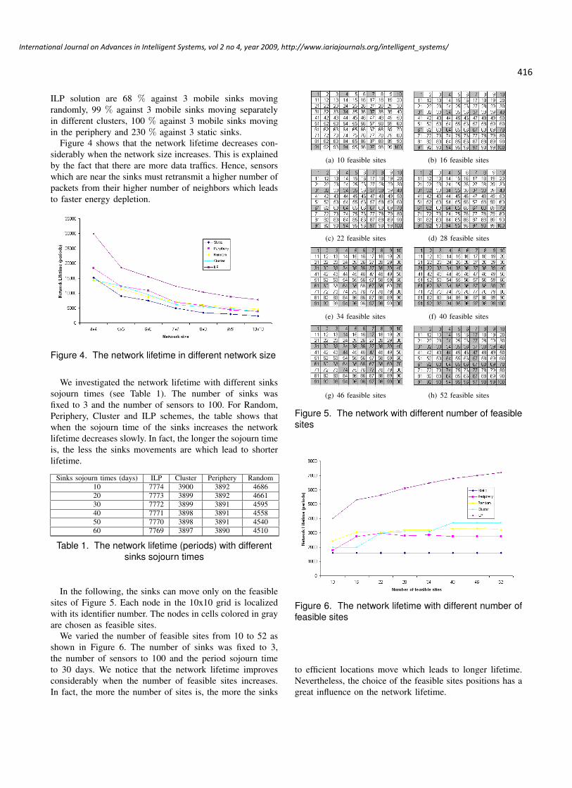
416


ILP solution are 68 % against 3 mobile sinks movingrandomly, 99 % against 3 mobile sinks moving separatelyin different clusters, 100 % against 3 mobile sinks movingin the periphery and 230 % against 3 static sinks.

Figure 4 shows that the network lifetime decreases con-siderably when the network size increases. This is explainedby the fact that there are more data traffics. Hence, sensorswhich are near the sinks must retransmit a higher number ofpackets from their higher number of neighbors which leadsto faster energy depletion.

Figure 4. The network lifetime in different network size

We investigated the network lifetime with different sinkssojourn times (see Table 1). The number of sinks wasfixed to 3 and the number of sensors to 100. For Random,Periphery, Cluster and ILP schemes, the table shows thatwhen the sojourn time of the sinks increases the networklifetime decreases slowly. In fact, the longer the sojourn timeis, the less the sinks movements are which lead to shorterlifetime.

Sinks sojourn times (days) ILP Cluster Periphery Random10 7774 3900 3892 468620 7773 3899 3892 466130 7772 3899 3891 459540 7771 3898 3891 455850 7770 3898 3891 454060 7769 3897 3890 4510

Table 1. The network lifetime (periods) with differentsinks sojourn times

In the following, the sinks can move only on the feasiblesites of Figure 5. Each node in the 10x10 grid is localizedwith its identifier number. The nodes in cells colored in grayare chosen as feasible sites.

We varied the number of feasible sites from 10 to 52 asshown in Figure 6. The number of sinks was fixed to 3,the number of sensors to 100 and the period sojourn timeto 30 days. We notice that the network lifetime improvesconsiderably when the number of feasible sites increases.In fact, the more the number of sites is, the more the sinks

(a) 10 feasible sites (b) 16 feasible sites

(c) 22 feasible sites (d) 28 feasible sites

(e) 34 feasible sites (f) 40 feasible sites

(g) 46 feasible sites (h) 52 feasible sites

Figure 5. The network with different number of feasiblesites

Figure 6. The network lifetime with different number offeasible sites

to efficient locations move which leads to longer lifetime.Nevertheless, the choice of the feasible sites positions has agreat influence on the network lifetime.

417


5.2. The Sinks Sojourn Times

We studied the pattern of the distribution of the sinkssojourn times at the different nodes. All the nodes of the gridcan be feasible sites. Figures 7, 8, 9, 10, and 11 show thesojourn times of three sinks in 10x10 grid for respectivelyStatic, Periphery, Random, Cluster and ILP schemes.

Figure 7. Sinks sojourn times at the different nodes of10x10 grid network with Static scheme

Figure 8. Sinks sojourn times at the different nodes of10x10 grid network with Periphery scheme

Figure 9. Sinks sojourn times at the different nodes of10x10 grid network with Random scheme

The optimal sinks locations obtained for static sinks arethe nodes which are almost at minimum distance i.e., numberof hops to all other nodes. In Random scheme, the sinkssojourn time is variably distributed among all the nodes ofthe network. In the Periphery scheme, it is fairly distributed

Figure 10. Sinks sojourn times at the different nodes of10x10 grid network with Cluster scheme

Figure 11. Sinks sojourn times at the different nodes of10x10 grid network with ILP scheme

among the nodes in the perimeter of the network. For theCluster scheme, the grid 10x10 was divided in 3 clusters3x10, 3x10 and 4x10 in which the sinks move separately.We notice that the sink sojourns most of the times at thecorners and the central grid area of its cluster. In the ILPscheme where the sinks move in the entire network, the samepattern is obtained, the sinks sojourn most of the times atthe corners and the central grid area as shown in Figure 11.

Independently of the size of the network and the numberof the sinks as shown in Figure 12 and 13, the optimallocations of the sinks according to ILP solution are the fourcorners of the grid, then the central grid area. The sojournof the sinks at the central grid area can be explained asfollows. If one of the sinks is located in the center of the gridit will have four neighbors within the transmission range.Contrarily, if it is located in the perimeter or the corner, itwill have respectively three and two neighbors. Obviously,the more neighbors within the transmission range the sinkhas, the better the traffic load balanced among nodes is andthe higher lifetime is. However, independently of where thesinks are located, the sensors in the corners drain less energyon forwarding packets than the sensors in the center whichare always along a routing path to reach the sinks. For thisreason, the sinks sojourn more at the nodes in the cornersthan the nodes in the central grid area in order to consumethe residual energy of the ”rich” sensors.

418


Figure 12. ILP sinks sojourn times at the different nodesof 8x8 grid network

Figure 13. ILP sinks sojourn times at the different nodesof 9x9 grid network

5.3. The energy distribution

We analyzed the impact of the five schemes on the energyconsumption at lifetime end in a network with 3 mobile sinksand 100 sensors. The distribution of energy consumptionwhen the first sensor dies is depicted in Figures 14(a),15(a), 17(a), 16(a) and 18(a). A light color means a higherpercentage of energy consumption.

It is remarkable in all the figures that the energy consump-tion is highly variable and depends on the sinks locations.We notice that the nodes near the sinks have relatively higherenergy consumption compared to most of the others becausethey have to receive and relay all other neighbors data inaddition to their own data. This leads them to consume moreenergy.

In Figure 14(a), we observe that higher percentage ofenergy consumption is concentrated around three nodesin the grid which are the locations of the static sinkswhereas the other sensors have a lower amount of energyconsumption (dark color).

When the sinks move on the periphery of the network, thehighest energy consumption occurs in nodes closest to theboundary of the network while the others nodes specially inthe center consume less energy as seen in Figure 15(a).

In the Cluster scheme as shown in the Figure 16, theenergy consumption is only balanced among the nodes ofevery cluster and not in the whole network. This is becauseof the restriction of sinks mobility to theirs clusters.

Figure 17(a) shows that Random scheme results in a better

(a) Energy consumption

(b) Residual energy

Figure 14. Static scheme in 10x10 grid network


(b) Residual energy

Figure 15. Periphery scheme in 10x10 grid network

419



(b) Residual energy

Figure 16. Cluster scheme in 10x10 grid network


(b) Residual energy

Figure 17. Random scheme in 10x10 grid network


(b) Residual energy

Figure 18. ILP scheme in 10x10 grid network

balancing of energy consumption than Static, Periphery andCluster schemes. In fact, we notice a larger area with lightcolor.

However, ILP scheme balances almost perfectly the en-ergy consumption among the nodes. In fact, the majority ofthe nodes depleted their energy at the same time except thefour corners as shown in Figure 18(a).

The distribution of the residual energy at each sensor nodein 10x10 grid with 3 mobiles sinks was also studied (seeFigures 14(b), 15(b), 17(b), 16(b) and 18(b)).

With static sinks, the majority of sensors have moreresidual energy at the end of network lifetime than theschemes with mobile sinks which have their initial energiesmore depleted at the lifetime end.

For the ILP scheme, sensor nodes have less residualenergy than in the case of sinks moving in clusters. Thisis due to the fact that the mobility of sinks in the wholenetwork changes the nodes acting as relays frequently andleads to balanced energy consumption among nodes. While,in the Cluster scheme, the movement of the sinks is restrictedto their own clusters. So, this approach prevents to haveglobal view of the entire network.

The ILP scheme results in a better distribution of residualenergy among the nodes compared to Cluster, Periphery,Random and Static schemes. The results show that thepercentages of the residual energy that remain unused at thenetwork lifetime end for Static, Periphery, Random, Clusterand ILP schemes are respectively 71 %, 45 %, 31 %, 31%, 3 %. Moreover, the number of sensors which have morethan 50 % of their initial energies left at lifetime end is 80,

420


36, 20, 27 and 4 respectively for Static, Periphery, Random,Cluster and ILP schemes

It is remarkable in the ILP scheme, as shown in the Figure18(b), that the sensor nodes in the corners have higher energyat the end of network lifetime than the others nodes. This canbe explained by the fact that they do not drain their energyin forwarding neighbor’s data in addition to their own data.

Moreover, we observe that at the end of network lifetimethe distribution of residual energy in the grid is more bal-anced among the nodes when the number of sinks increases(See Figure 19). The use of more sinks results in thereduction of the average path length between the sensorsand sinks thus enabling to achieve less traffic load to thenodes and increased network lifetime.

(a) 2 sinks (b) 3 sinks

(c) 4 sinks

Figure 19. Residual energy distribution of ILP schemein 5x5 grid network with increasing number of sinks

These results are interesting since they are not puretheory. We tried to approach realistic buildings deploymentparameters in our assumptions and especially with sinks thatcan not move frequently.

6. Conclusion and future Work

In this paper, we have explored the problem of positioningmultiple mobile sinks in wireless sensor networks insidebuildings, in order to avoid the energy hole problem andextend the network lifetime, which is really needed inpractice.

As a solution, we have proposed an ILP which directlymaximizes the network lifetime instead of minimizing theenergy consumption or maximizing the residual energy,which is what was done in previous solutions. The proposedILP determines the best way to relocate sinks by giving theiroptimal locations and the duration of their sojourn time.

A comparative study of the proposed solution with staticsinks, mobile sinks moving in the periphery of the network,mobile sinks moving randomly and mobile sinks movingseparately in different clusters was made. Relocating sinkswith our solution and using realistic parameters assumptionsresults in the sensor network lifetime extension and theenergy consumption more balanced among the nodes. Thelifetime improvements achieved in our experiments by de-ploying 3 mobile sinks in the network with hundred sensorsare almost 99 % against 3 mobile sinks moving separatelyin different clusters and almost 230 % against 3 static sinks.

The study of the pattern of the distribution of the sinksat different locations showed that the sinks sojourn mostof times at the nodes in the central grid area and in thecorners. This corresponds to very interesting feasible sitesin buildings because the sinks can be easily relocated in thecorridors which are often in the center of the buildings andprovided with power and Internet access.

The weakness of the proposed approach is the scalabilityproblem in networks with thousands of sensors due tothe high ILP resolution complexity. In order to adopt thissolution in a large scale wireless sensor network with morethan hundreds of sensors, the network might be divided inseveral sensor sub-networks which will be deployed in theeach part of the building. More than one sink can then beplaced inside each zone to collect the information of thein-door environment. To implement the solution in a realenvironment and apply the model in real time conditions,technicians will be in charge of relocating the mobile sinksin the open areas of the buildings after long periods (i.e.,months).

In our future work, we intend to improve the proposedILP by including parameters and constraints that modelmore realistic requirements of an indoor environment (e.g.,collisions) and take into account the energy consumption ofsensing and data processing. We envisage also to introduceoptimization in data routing by considering relevant metricslike latency, control overhead.

References

[1] L. Ben Saad and B. Tourancheau, “Multiple mobile sinkspositioning in wireless sensor networks for buildings,” in3 rd International Conference on Sensor Technologies andApplications SensorComm, 2009.

[2] J. Pan, Y. T. Hou, L. Cai, Y. Shi, and S. X. Shen, “Topologycontrol for wireless sensor networks,” in Proceedings of the9th annual international conference on Mobile computing andnetworking MobiCom, 2003, pp. 286–299.

[3] X. yang Li, W. zhan Song, and Y. Wang, “Topology controlin heterogeneous wireless networks: Problems and solutions,”in Proceedings of the 23rd Joint Conference of the IEEEComputer and Communications Societies INFOCOM, 2004.

421


[4] A. Sankar and Z. Liu, “Maximum lifetime routing in wirelessad-hoc networks,” in Proceedings of the 23rd Annual JointConference of the IEEE Computer and Communications So-cieties INFOCOM, vol. 2, 2004, pp. 1089–1097.

[5] K. Fodor and A. Vidacs, “Efficient routing to mobile sinksin wireless sensor networks,” in WICON ’07: Proceedings ofthe 3rd international conference on Wireless internet. ICST,Brussels, Belgium, Belgium: ICST (Institute for ComputerSciences, Social-Informatics and Telecommunications Engi-neering), 2007, pp. 1–7.

[6] O. Younis and S. Fahmy, “Distributed clustering in ad-hocsensor networks: A hybrid, energy-efficient approach,” inProceedings of the 23rd Annual Joint Conference of the IEEEComputer and Communications Societies INFOCOM, 2004,pp. 629–640.

[7] S. R. Gandham, M. Dawande, R. Prakash, and S. Venkatesan,“Energy efficient schemes for wireless sensor networks withmultiple mobile base stations,” The IEEE Global Telecommu-nications Conference GLOBECOM, 2003.

[8] W. Alsalih, S. Akl, and H. Hassanein, “Placement of multiplemobile base stations in wireless sensor networks,” IEEE In-ternational Symposium on Signal Processing and InformationTechnology, 2007.

[9] X. Wu, G. Chen, and S. K. Das, “Avoiding energy holes inwireless sensor networks with nonuniform node distribution,”IEEE Transactions on Parallel and Distributed Systems, 2008.

[10] ——, “On the energy hole problem of nonuniform nodedistribution in wireless sensor networks,” IEEE InternationalConference on Mobile Adhoc and Sensor Systems MASS,2006.

[11] J. Lian, K. Naik, and G. B. Agnew, “Data capacity improve-ment of wireless sensor networks using non-uniform sensordistribution,” in International Journal of Distributed SensorNetworks, 2005.

[12] A. Bogdanov, E. Maneva, and S. Riesenfeld, “Power-awarebase station positioning for sensor networks,” in Proceedingsof the IEEE INFOCOM, 2004, pp. 575–585.

[13] E. Oyman and C. Ersoy, “Multiple sink network designproblem in large scale wireless sensor networks,” IEEE In-ternational Conference on Communications, 2004.

[14] H. Kim, Y. Seok, N. Choi, Y. Choi, and T. Kwon, “Optimalmulti-sink positioning and energy-efficient routing in wirelesssensor networks,” Lecture Notes in Computer Science LNCS,2005.

[15] J. Luo and J.-P. Hubaux, “Joint mobility and routing for life-time elongation in wireless sensor networks,” In Proceedings24th Annual Joint Conference of the IEEE Computer andCommunications Societies INFOCOM., 2005.

[16] K. Akkaya and M. Younis, “Sink repositioning for enhancedperformance in wireless sensor networks,” Elsevier ComputerNetworks Journal, 2005.

[17] B. Wang, D. Xie, C. Chen, J. Ma, and S. Cheng, “Employingmobile sink in event-driven wireless sensor networks,” IEEEVehicular Technology Conference VTC, 2008.

[18] Z. M. Wang, S. Basagni, E. Melachrinoudis, and C. Petrioli,“Exploiting sink mobility for maximizing sensor networkslifetime,” In Proceedings of the 38th Annual Hawaii Inter-national Conference on System Sciences HICSS, 2005.

[19] S. Basagni, A. Carosi, E. Melachrinoudis, C. Petrioli, andZ. M. Wang, “Controlled sink mobility for prolonging wire-less sensor networks lifetime,” Wireless Networks, 2007.

[20] Y. Bi, J. Niu, L. Sun, W. Huangfu, and Y. Sun, “Mov-ing schemes for mobile sinks in wireless sensor networks,”Performance, Computing, and Communications Conference,2007.

[21] R. C. Shah, S. Roy, S. Jain, and W. Brunette, “Data mules:Modeling a three-tier architecture for sparse sensor networks,”in IEEE International Workshop on Sensor Network Protocolsand Applications SNPA, 2003, pp. 30–41.

[22] M. Marta and M. Cardei, “Improved sensor network lifetimewith multiple mobile sinks,” Pervasive and Mobile computing,2009.

[23] Z. Vincze, R. Vida, and A. Vidacs, “Deploying multiple sinksin multi-hop wireless sensor networks,” IEEE InternationalConference on Pervasive Services, 2007.

[24] A. Azad and A. Chockalingam, “Mobile base stations place-ment and energy aware routing in wireless sensor networks,”IEEE Wireless Communications and Networking ConferenceWCNC, 2006.

[25] D. Maniezzo, K. Yao, and G. Mazzini, “Energetic trade-offbetween computing and communication resource in multi-media surveillance sensor network,” 4th IEEE Conferenceon Mobile and Wireless Communications Networks MWCN,2002.

[26] CPLEX http://www.ilog.fr/products/cplex/.

[27] Chipcon. CC2420 2.4 GHZ IEEE 802.15.4 / ZigBee-readyRF transceiver, 2004.

422


Spatial Diversity Solutions for Short Range Communication in Home CareSystems using One Antenna Element

Markku J. Rossi, Jukka Ripatti, Fikret Jakupovic and * Reijo EkmanMikkeli University of Applied Sciences, Finland* Turku University of Applied Sciences, Finland

[email protected]

Abstract- It is becoming increasingly important for coun-tries like Japan, Finland and Italy to enable as wide aspossible home care for their elderly citizens because of therapidly changing age structure of the population and highhospital costs. Wireless sensors hidden in furnishings ( as areference to a Finnish ongoing project ) can provide neces-sary information for the high quality planning of homecare visits. The relative positions of the radios are now fixedbecause of their relations to the furnishings. When conduc-tive or metallic walls, floors or objects are found in theapartment, an antenna can hit a radio fade caused by shad-owing or the summing up of waves. The Link Quality Indi-cator of a ZigBee® receiver can vary by up to 50 unitswithin a short distance because of the floor, compromisingthe radio range. This paper describes the principles of aradio construction which is able to move the antenna ele-ment inside the enclosure of the radio unit along an X-shaped path along the major mechanical plane of the radiounit. Two electrical motors dynamically optimise the loca-tion of the internal antenna element to fit the current radiopropagation environment. The paper also describes thefeasibility and cost factors associated with the new struc-ture. The achieved effect is a useful countermeasureagainst shadowing and multipath in the 2.44 GHz band butprovides only a partial solution to the problem in the 868MHz band, due to the space limitations in a typical radiounit. A prototype of the Diversity Adaptability radio wasbuilt and the capability to remarkably enhance the receivedpower in difficult fading conditions was verified in ananechoic chamber. The observed side effects to the direc-tional pattern of the radio were analysed to be removable bycarefully selecting the route of the coaxial cable from theradio unit to the moving antenna element.

Keywords-home care; short range radio; sensors; ZigBee;shadowing; fading; spatial diversity; avoiding gain minima;diversity adaptability

I. INTRODUCTION

Mikkeli University of Applied Sciences ( MiUAS ) issituated in the South-Eastern district of Finland thathas one of the most challenging predicted demographicstructures for the 2020s in Europe. The eastern part ofthe district is expected to have 44700 inhabitants in2020, 2130 of which will need daily care, 1580 be-cause of memory disorders . The age structure of thepopulation can be characterised by calculating whatproportion of the population is children and of over 65years old, divided by the number of people that are inthe working age. The fresh population forecast gives aratio 75,3% for Eastern Finland for 2020 /17/ . Thesituation will be more challenging for Eastern Finlandthan to the whole Finland. In Finland the ratio iscaused by the unusually high birth rates in 1945 – 1955and in Italy and Japan by the low birth rates after 1980.The forecasted population structures of these countriesshow challenges in financing the health care for theelderly [18].

0

2000000

4000000

6000000

8000000

10000000

Size of the

population

group

0-4 15-

19

30-

34

45-

49

60-

64

75-

79

90-

94

Age group

Population in Japan in 2020

Figure 1. A forecast of the population structure of Japan for 2020[18].

423


050000

100000150000200000250000300000350000400000

Size of the

population

group

0-4 15-

19

30-

34

45-

49

60-

64

75-

79

90-

94

Age group

Population in Finland in 2025

Figure 2. A forecast of the population structure of Finland for 2025[18].

0500000

10000001500000200000025000003000000350000040000004500000

Size of the

population

group

0-4 15-

19

30-

34

45-

49

60-

64

75-

79

90-

94

Age group

Population in Italy in 2040

Figure 3. A forecast of the population structure of Italy for 2040[18].

Data communication from homes has become feasi-ble due to GSM and Flash OFDM ( at 450 MHz )WWAN networks. Wireless communication has alsobecome feasible at homes due to low cost short rangeradios such as ZigBee ®. The MiUAS generated aninitiative to send to the hospital district home care visitrecommendations generated at a call centre and basedon real time event messages sent wirelessly from thehomes of the elderly [14]. The project is now financedby the ERDF instrument of the European StructuralFund ( ESF ) and governed locally. The project built37 test homes in 2 cities, 2 towns and 2 municipalities.We are aiming at 40% reduction in hospital days for aselected group due to increased home care, with corre-sponding cost savings. The main result will be the newwork process. Recommendations of action based onreal time sensor data have not been used in planning ofhome visits before. The decision rules for extractingrecommendations of action from sensor data will alsobe new. The main technical challenges are how tomaximise the time between replacing batteries to thesensor that detects motion in the living room and byproviding countermeasures to the effects of RF shad-owing and fading. Otherwise the ZigBee technology isalready quite field proven, e.g. in the U.S. networks

that read kWh-readings of consumed electricity fromhomes. The first challenge is related to different tacticsto keep the receiver circuitry of the sensor device on aslittle as possible. The second challenge is related to thesituation when the transmitter of the device is transmit-ting sensor data in an environment with shadowing.The battery life aspect was addressed in [2].

II. MOBILE CARE IN EASTERNFINLAND PROJECT

The Mobile Care service will produce three kinds ofproducts: alarms, emergency voice calls and recom-mendations of actions, like home care visits. The op-erators generating recommendations can view the fol-lowing events:

- usage of a selected electrical appliance , such as amicrowave oven

- motion in the living room- pressure distribution on the bed- whether the main door is opened or shut- usage of the electrical cooker- verification of taking medication pills out of

a smart pill box- whether the inhabitant is inside / outside of the

apartment.

The homes have VoIP handsets with one buttoncall initiation. The Central Unit has both a WWANradio and a WLAN base station in addition to ZigBee.This also enables IP cameras. A ZigBee wrist devicewith an alarm button completes the set [14]. The re-cently founded company IsCom Oy continues the workof Riihonlahti Services Ltd in the project. The projectstarted a field test with 37 homes in October 2009. Thefinal project report is expected in April 2010.

A plan for the next phase includes a project thattakes UML descriptions of the decision rules of creat-ing action recommendations out of sensor data ( aresult of the current project ) and develops an expertsystem that will deliver recommendations semi-automatically under the supervision of a nurse. MiUASis now also a partner of a funding proposal to the EUCOST programme for deep co-operation between or-ganisations that have similar goals than MiUAS in thefield of Smart Homes oriented to Health. The proposalwas filed in September 2009 by Coventry University.

424


III. RESEARCH NEEDS FOR REACHINGTHE REQUIRED LEVELS OFRELIABILITY

The error control methods: error control coding andretransmissions operate on a single wireless channeland add redundancy to the data packets to improvereliability. Their usefulness is however sometimescompromised over real fading RF channels. If thepacket transmission both starts and passes the packetdeadline in a deep fade, the methods mentioned beforeare usually not successful in delivering the packet [8].

The former reference is convinced that the incorpo-ration of the spatial diversity approach into error-control is a very promising approach.

In the Mobile Care Eastern Finland concept some ofthe sensors can be invisibly embedded into furnishings.This eliminates the possibility of moving the sensorradio slightly so that heavy shadowing or a heavy slowfading can be avoided. We then decided to study spa-tial diversity to achieve as high as possible reliabilityin delivering the measurement results of the sensors.This is particularly important with the bed pressuredistribution sensor. The later applications of this sensorcan include e.g. an analysis of the breathing parametersduring sleep.

IV. RADIO PROPAGATION ENVIRON-MENTS RELATED TO USAGE ATHOMES OF THE ELDERLY

A typical home where we are expecting to use theMobile Care service in Eastern Finland is a woodensingle family house. Typical dimensions for this housetype are: floor area 8 x 8 m, a second floor with nar-rower rooms 2.7 m above the first floor and a fireplacedownstairs built of bricks. The radio propagation herethrough the structures at 2.4 GHz has a fairly low levelof shadowing. The findings in [7] support this conclu-sion. The metal casing above the stove and by thechimney typically cause some effects.

Another frequency available in Finland is 868.3MHz according to the standard EN 300 220-1, with alonger range than for the ISM band with a 1 mWtransmit power.

It is however also common that the inhabitant livesin a block of flats with steel reinforced concrete wallsand floors. There is some heavy shadowing and reflec-tions present particularly due to washing machines,water pipes and dish washers.

The reference [4] examined an office space of 30 x15 m and found that the attenuation caused by a 0.14 mthick concrete wall was in the order of 5 dB.

The reference [5] uses the parameter Link QualityIndicator LQI to describe propagation effects. The LQIwas interpreted there to represent well the chip errorrate. In the case of a floor consisting of wood and poly-styrene, sharp variations in LQI , 50 units out of thetotal range of 255 units along a 0.25 metre section ofthe propagation path were detected. The dielectricconstant of polystyrene at 1 MHz is of the order of2.75 [9]. The bending of radio waves is heavily corre-lated with the dielectric constant. It is evident thatmore studies would be needed on the effects of floorcoverings made of different dielectric plastics materi-als.

In [6] measurements of RSSI ( Received SignalStrength Indicator ) were performed up to a distance of32 metres in an indoor scenario. The Packet Error Rate( PER ) was found to be low until the distance reached25 metres. Severe degradation of 802.15.4 was how-ever detected in the active space of a 802.11b/g( WLAN ) base station, if the WLAN channels and theSRR ( Short Range Radio ) frequencies overlapped.There are however at least 4 pieces of 802.15.4 chan-nels not severely overlapping with the 802.11b/g chan-nels. The WLAN usage is at the moment very commonin Finnish blocks of flats.

The rationale to study a solution that can move theantenna element to various positions inside the deviceis based on the characteristics of current two-elementdiversity antennas. These antennas have two elementsat fixed positions from each other. The reference [3]points out that when the distance between the edges ofthe antenna elements is e.g. 41.7 mm ( very suitable forour purpose ), the gain of the combination has gainminima -22 dB .. -18 dB deep on the horizontal planeas can be predicted from the theory of antenna arrays.We want to avoid the existence of these gain minima.

V. THE SPATIAL DIVERSITY SOLUTION

The design parameters of the 802.15.4 are wellsuited to our usage scenario because our expectedrequired ranges as such are nearly always less than 25metres. The challenge is mostly related to slow fadingcaused by the summing of the signals related to a directpath and reflections from metal surfaces.

The fitting of the sensor/radio devices discreetlyinto furnishings usually prevents the moving of thedevice with a built in antenna element which is re-quired to avoid a deep fade. We decided to study thepossibility of arranging spatial diversity that would beinternal to the device and be arranged with only one

425


antenna element to minimise antenna, signal divisionand cabling costs in addition to avoiding gain minimaat certain angles. No prior art studies about antennaelements moving inside the enclosure of a device, inconnection with sensors for home care were found.

The typical device dimensions of a combined sen-sor, logic and RF circuitry are 50 x 50 mm without thebattery compartment [10]. Willig [8] mentions thatantenna movements of even a few centimetres areadequate to change the value of the spatial autocovari-ance function. The half wavelength in the ISM band isaround 62 mm. If we move the antenna element alonga path with a 45 degree angle to the sides of the enclo-sure, the available movement is of the order of 70 mmin an enclosure also housing a typical 2500 mm2printed circuit board.

Benefits found in printed circuit antennas include:narrow bandwidth, mechanical strength, low cubicvolume and low cost. A modern antenna design ispresented in [3]. The bandwidth of a Hilbert inverted-F-antenna ( IFA ) for 2400 MHz is 3.3% or 80 MHz.This fits well with a scenario where we would use the5th and the 10th channel of 802.15.4 so that they fall inbetween two wider WLAN channels. The WLANchannels are however this narrow only in the U.S., andin Europe wider WLAN channels are admitted, bring-ing more spectral overlapping to ZigBee and WLAN.These particular ZigBee channels are separated by 25MHz. The Hilbert IFA would then reject the majorparts of two WLAN channels and amplify only WLANchannel 6 and the two selected ZigBee channels. Thedimensions of this Hilbert IFA are 2.7 x 5.6 x 1.5 mmand the gain is 1.0 – 1.5 dBi.

The mechanical construction consists of a plasticboard with the movement route holes above the circuitboard, with the flexible antenna coaxial cable attachedto the centre of the circuit board.

Springs are attached to the 90 degree and 270 de-gree corners of the plastic board. Opposite to thesprings there are two miniature electric motors. TheKysan Electronics FF-K10WA-5Z215 miniature motorhas an 11.5 mm long chassis. It provides 0.06 mN/mtorque at 14000 rpm and 0.09 W [11]. If the used pul-ley has a diameter of 3 mm, the required spooling for a70 mm displacement is 7 full turns and the spoolingtime is 30 milliseconds. The other dimensions of themotor are: 6 x 8 mm. The antenna element slides alongthe X-shaped path drawn by one of the motors at atime. Whenever one motor is moving the antennasledge the other motor is idle.

The antenna sledge is attached to both springs andboth motors via lines. The basic orientation is with thesledge at the crossing of the two paths. The forceagainst the spring is 0.04 N and the desired springconstant is 0.1 N/m, slightly less than the motor can

stretch. The small pulleys for the motors can hold theline attached to the sledge.

When the antenna diversity module is 60 x 60 mm,the routes ( 2 ) of the sledge at 45 degree angles can be70 mm long each, forming together an X-shapedmovement area. This means that the length of the routefrom one end of the route to the centre is 35 mm andthe maximum additional movement to any of the re-maining three corners is also 35 mm .

When the sledge is moving, the motor that is notpulling the line, is releasing a maximum of 70 mm ofline. The springs are capable of overcoming the slidingfriction of the sledge. Therefore the sledge has also amicro sized servo in it to stop the movement whereverthis is needed.

An example of a state-of-the-art servo is the Picofrom GWS [12]. The dimensions are: 22.8 x 9.5 x 15.5mm and the axle turns 60 degrees in 0.12 seconds. Theactivated servo will lock the sledge at the desired posi-tion against the pull of the springs.

When used together with the frequency of 868.3MHz, the ratio of the dimension of the path of theantenna movement to the wavelength is only 0.2. It isthen uncertain that the maximum improvement in thefield strength would be as high as if operating at 2.44GHz.

VI. EFFECTS ON THE SENSORDEVICES FROM THE ADDEDDIVERSITY ADAPTABILITYFUNCTION

The coupling of the interference ( EMI ) from thedigital circuits to the antenna is considerable in relationto the reception. The sharp edges of digital signalsgenerate interference energy at high frequencies. Thenonlinearities of the receiver can leak this energy intothe received signal due to nonlinear mixing results. Asensitive receiver with fast digital circuits nearby istherefore usually a result of an iterative designing andprototyping process.

Now as we are moving the antenna unit above thelogic circuits, the design of the electronic module ismore challenging than ever. The complexity of thecircuitry is however much lower than in a 3G cellularphone with fast processing and a GPS receiver.

Because of the Diversity Adaptability function thecubic volume of the wireless sensor device grows big-ger. The effect from the empty space in between theelectronics board and the plastic board is 36 cm3 if weallow 10 mm vertical space for the flexible coaxialcable for movement during the optimisation of thereception. The two motors consume 1.1 cm3 of spaceand the servo 3.4 cm3. The required space for the an-

426


tenna sledge compartment can be estimated to be 18cm3. This can be compared with the volume of an AAsized primary battery, 8 cm3. Because our advanceddevice is now larger than a standard device, it is moredifficult to hide it in certain kinds of furnishings.

The additional cost is: two motors 4.9 € , servo 10.8€ and cables plus additional mechanical gear and alarger enclosure 1 €, bringing the additional cost to16.7 €. This means roughly doubling the componentcost of the wireless sensor device. When compared tothe new ability to dynamically minimise the packeterror rate of ZigBee in changing propagation environ-ments, the extra cost can sometimes be acceptable.

VII. CONCLUSIONS FOR THETHEORETICAL CONCEPT

The critical nature of delivering sensor measure-ment results reliably in a service assisting the planningof medical home care visits generated a concept whereone single antenna element is moving inside the wire-less sensor device to minimise the packet error rate.The optimisation can adapt to a changing environmentsuch as the later positioning of new home appliances inor out of the line-of-sight paths between the radios.

The concept shows theoretical promise to help insituations where the location of the sensor devices isfixed and cannot be fine tuned to avoid fades. Thecomponent cost of the device is doubled as is its cubicvolume when compared to a conventional device.

A clear benefit of the solution compared to a com-peting scenario, the two-element diversity antenna, isthe absence of gain minima at certain angles, associ-ated with the pair of antenna elements.

I also recognised the need for more study on the ef-fects of dielectric floor coverings to ZigBee propaga-tion due to the possible bending of waves in the floorcoverings.

VIII. DESIGNING A PROTOTYPE FOR THEDIVERSITY AVAILABILITY ( DA ) FUNCTION

The design of the prototype was based on the princi-ple presented at the 3rd International Conference onSensor Technologies and Applications /1/ , ( FIG 4).

This article describes a real transceiver pair designedand built according to the concept from [1] and aboutits measured performance. From the wide selection ofcommercial ZigBee modules we chose devices fromthe product line of Dresden Elektronik Ingenieurtech-nik GmbH in Germany. The unit providing an interfaceto the PC and to an external antenna is called the Sen-sor Terminal Board ( STB ). The dimensions are 100 x75 mm. It has connectors for the actual radio board.

The radio board is called the Radio Controller BoardRCB230SMA. It has horizontal dimensions of 53 x 52mm coming very close to our previous size assump-tions.

Figure 4. DA realised with two motors pulling a sledge againstsprings. The sledge has a servo for braking and an antenna elementon it.

The radio Controller Board is capable of transmittingat +3 dBm. The transceiver chip is the AtmelAT86RF230. The board manufacturer gave us greatco-operation and programmed the two STBs to use aconstant frequency of 2,44 GHz and a transmit powerof -10 dBm. These parameters would be suitable forthe later tests in an anechoic chamber. In addition, theSTB that would be selected to be the network deviceand receiving continuous temperature measurementdata from the coordinator device was capable of out-putting its own RSSI ( Received Signal Strength Indi-cator ) measurement results continuously and at suit-able 1 second intervals to the USB connector.

The prototype of the network device uses a flat chipantenna instead of a higher quarter wave stub as origi-nally planned. Samples of the interesting Hilbert IFA[3] are not available anymore so we selected a verysmall chip antenna from the manufacturer Yageo Cor-poration. Again, we received excellent co-operationand got samples of the Yageo 3216 PIFAs ( PlanarInverted-F ) antennas. Instead of the 2,7 x 5,6 mmdimensions from the original plan we now moved tothe 1,6 x 3,2 mm range. The mean effective gain forYageo is +0,14 dBi, slightly less than for the HilbertIFA of [3]. The directional pattern is not perfectlyomnidirectional as the maximum gain to a space angleis +3,7 dBi [13].

We then built the printed circuit board for the PIFAexactly according to the manufacturer’s recommenda-tions ( including the matching components ) and con-nected the antenna unit to the SMA coaxial connectorof the Dresden RCB used as a network device with a50 ohm cable of the type RG 178 B. The structure ofthe prototype network device can be seen from FIG. 5.A good feature of the construction is the 20 x 30 mm

427


printed circuit board for the PIFA, having a largeground plane visible on the picture against the elec-tronics situated underneath. For the measurements theantenna unit was turned 180 degrees vertically com-pared to this picture.

The servo is the same unit as selected earlier, theGWS Pico [12]. The motors of the prototype are Mo-traxx K10WAs from Motraxx Elektrogeraete GmbH.The specifications are very close to the ones fromKysan [11].

Figure 5. The DA antenna construction on Dresden RCB. The twomotors are visible. The servo for the braking function is underneaththe board which has the X-shaped hole.

IX. LABORATORY TESTARRANGEMENTS FOR THEPROTOTYPE

After investigating different service providers foranechoic chambers we selected the Turku University ofApplied Sciences’ chamber. Their facility is situated inSW Finland and uses a RFD-FA-100 room by ETS-Lindgren. The internal dimensions are : 6,4 m x 3,44 mx 3,0m (h). The level of internal reflections comparedto the direct wave is -20 dB. The overall appearance ofthe anechoic chamber can be seen in FIG. 6.

The distance between the transmitter and the DAreceiver was chosen to be 3,27 m. The height of thetransmitter antenna from the floor was 1,15 m and 1,00m at the receiver. The slight angle of 2,6 degrees forthe line connecting the antennas compared to horizon-tal does not affect the received power. The transmitterantenna was an omnidirectional quarter wave stub fromDresden Elektronik.

The room has a non-reflective turning table that canbe remote controlled from outside the chamber.

Figure 6. The anechoic chamber in Turku.

X. LABORATORY TEST RESULTS

The simulated condition of a severe signal minimumcaused by multipath was created with one 0,6 x 1,2 maluminium plate hanging vertically and at a 90 degreehorizontal angle compared to the signal path. Theachieved weakening of the signal was 17dB.

The ZigBee radio working as a coordinator is seen inFIG. 7.

Figure 7. The ZigBee coordinator radio in the anechoic chamber.

The DA effect was achieved by selecting 8 adaptationpositions for the DA antenna unit that is capable ofmoving along the X-shaped path. The direction“North” was at the receiver directly away from thetransmitter antenna. The DA positions were named asNE ½ , NE1, SE ½ , SE1, SW ½ , SW1 , NW ½ andNW1. The positions “ ½ “ were halfway from the cen-

428


tre of the X towards the ends of one of the four 35 mmlong DA paths. The positions “ 1 “ were 35 mm awayfrom the centre of the X.

The results of the test for achieving escape from thefade are in TABLE 1 :

Measurementno.

DA position RSSI ( dBm )

DA0 middle of the X -78DA1 NE ½ -67DA2 NE1 -70DA3 SE ½ -64DA4 SE 1 -63DA5 SW ½ -59DA6 SW1 -67DA7 NW ½ -79DA8 NW1 -62DA9 middle of the X -74

Table 1. The RSSIs when using the DA function. The unrotatedRSSI before providing the back reflector was -59 dBm.

The elapsed time between DA0 and DA9 was 10minutes. The usage of only one reflector caused a hys-teresis of 4 dB during the DA test ( -74 dBm - -78dBm).

The DA function was able to raise the RSSI by atleast 15 – 19 dB. The best position for this test settingwas the DA position SW ½ . The rotation of the an-tenna element during the linear movement was negligi-ble and as we can see from the second measurementdescribed below, the angular response at the anglesclose to the angle used in the test above was nearly flat.

The second test was the examination of the direc-tional pattern of the DA unit antenna gain against thehorizontal rotation angle.

The ZigBee network device on the electrically ro-tatable measurement table can be seen in FIG. 8.

The measurements were taken every 5 degrees, rotat-ing clockwise when seen from above the DA unit withthe starting point RSSI-0 pointing directly away fromthe transmitter antenna. The average RSSI over 72measurements over the angles was -62,3 dBm. Theaverage of the standard deviations of the powers atangles was 0.45 dB when the sample size at everyangle was 20 samples. The dBm-readings were thenrounded to the nearest 0.5 dBm reading to the table,because the radio gave the individual readings to theterminal emulation software only at a resolution of 1dBm. The typical 90% confidence level of the power

readings at the angles from the t-distribution with thesample size 20 is + - 0.78 dB.

Figure 8. The ZigBee network device on the electrically rotatablemeasurement table.

The results of the measurement of the horizontalangular response of the prototype are in TABLE 2 :

rotationangle,degrees

receivedpower,dBm

stddevia-tion,dB

rota-tionangle,de-grees

re-ceivedpower,dBm

stddevia-tion,dB

0 -59 .497 185 -66 .515 -58 .497 190 -64 .38410 -58 .357 195 -64 .44715 -56 .384 200 -62 .38420 -55 .447 205 -61 .38425 -55 .447 210 -61 .38430 -54.5 .49 215 -60 .38435 -54 .6 220 -59 .31640 -54 .477 225 -58 .38445 -54 .316 230 -58 .38450 -54.5 .497 235 -59 .38455 -55 .384 240 -58 .44760 -58.5 .49 245 -58 .43665 -61 .447 250 -59 .44770 -66 .548 255 -60 .38475 -70 .775 260 -58 .38480 -67 .632 265 -58 .38485 -65 .539 270 -58 .21890 -63 .316 275 -60.5 .49795 -61 .316 280 -61 .477100 -61 .384 285 -61.5 .589105 -62.5 .49 290 -62.5 .592110 -64 .447 295 -64 .384

429


115 -67 .316 300 -64 .436120 -70 .539 305 -64 .6125 -82 .853 310 -62 .384130 -74.5 .589 315 -62.5 .477135 -67 .447 320 -64 .497140 -67 .316 325 -67 .548145 -69.5 .654 330 -64 .316150 -67 .384 335 -62.5 .477155 -64 .384 340 -61.5 .583160 -66 .384 345 -61 .384165 -67 .384 350 -61 .477170 -67 .51 355 -61 .384175 -70 .624 360 -59 .316180 -66.5 .497

Table 2. The RSSIs of the DA prototype at different horizontalrotation angles.

These results can be seen also in polar format on FIG.9.

The diagram shows the numbers of the rotationmeasurement stops from RSSI-0 to RSSI-73 withRSSI-0 and RSSI-73 at the same angle.

When compared to the specification of the Yaego3216 PIFA which itself is not perfectly omnidirec-tional, we observed one new gain minimum caused bythe construction of the DA unit prototype. The gainminimum corresponding to the rotation angle of 125degrees caused an RSSI of -82 dBm. With the rotationangles of 120 and 130 degrees, the gain was alreadymore than 10 dB higher.

Directional pattern

-35

-30

-25

-20

-15

-10

-5

0

12 3 4 5 6

78

910

111213

141516171819202122

2324

2526

2728

2930

313233343536

373839404142

4344

4546

4748

4950

51525354555657585960

6162

6364

6566

676869707172

Figure 9. The directional pattern of the DA unit. The reference level0 dB corresponds to an RSSI of -50 dBm.

The average received power was at -62,3 dBm. Whenthe parameters :

Tx transmit power -10 dBm Tx antenna gain 0 dBi average Rx antenna element gain +0,14 dBi distance between the Tx and Rx antenna ele-

ments 3,27 metres frequency of 2,44 GHz

are applied to the Friis free space equation

received

P =dtransmitte

P *2 RxTx GG 2

4 r

we get receivedP = 923E-9 mW = -60,3 dBm .

When also taking into account the loss in the RG 178B coaxial cable between the Dresden RCB and theYaego antenna element of 1,6 dB, we notice that thereceived power was only 0,4 dB less than the theoreti-cal prediction. Actually the received power was thesame as the predicted power within the measurementaccuracy of the Atmel radio chip.

XI. ADDITIONAL MECHANICALPRINCIPLES

In addition to the current approach with one move-ment plane with one X-shaped path, the function canbe realised with two movement planes. The lowerplane has one straight hole in the horizontal directionof 45 degrees and is attached to an upper plane. Thewhole lower plane can move around a knob situatedbelow. The second, upper plane has a correspondingstraight hole at an angle of 135 degrees and can movealong the hole that is at a 90 degree angle with thelower hole.

The hole can also be circular in shape, e.g. from anangle of 3 degrees to 357 degrees. The antenna elementwould be attached to a pole corresponding to the handof a clock. The hand is attached to only one motor thatis situated at the centre of the circle.

If the original one-plane with two motors construc-tion is used, one additional release mechanism isneeded close to one of the springs. This mechanismselects the required one of two possible directions at 90degree angles to what the spring is pulling the antennasledge.

For practical control of the position with good longterm stability, a measurement of the position of the

430


sledge would be required for control feedback. Themeasurement can be optical, with an LED on the lowerside of the sledge and photodiodes attached to the radioboard under the movement plane.

XII. ENERGY MINIMISATION ASPECTSAND SHADOWING

The main addition to the energy consumption inthis concept compared to traditional solutions is duringthe running of the two Motraxx electrical motors one ata time. The usual starting position of the antennasledge is from the centre point of the x-shaped antennapath. The efficiency of the motors is at a maximumwith a 3.0 V supply voltage and with a 0.12 A current,providing rotation at 13800 RPM. The maximum dis-tance travelled by the sledge during the measurementphase is 4 times 70 mm, or 280 mm. After this, thesledge simply moves to the most optimal measuredposition in terms of the packet error rate. The averagedistance travelled then is 17.5 mm. The end stage ofthe motor driver circuit is a switching transistor with ahigh efficiency.

With the planned pulley each 10 mm sledge move-ment takes one turn of the axle and lasts for 4.3 ms.The length of the steps is 10 mm. To find a new opti-mum antenna position would take an average of 30steps. The duration of the whole procedure is domi-nated by the time to measure the new Received SignalStrength or the packet error rate and not by the move-ment periods of the antenna sledge.

The energy consumption of the motors during oneposition search is 3.0 V * 0.12 A * 30 * 0.0043 s =0.046 Ws. This can be compared to a typical batteryconfiguration with two pieces of CR123A Lithiumprimary batteries containing 9.0 Wh or 32400 Ws ofenergy. The position optimisation procedure is usuallynot a significant factor in the overall energy consump-tion.

Instead, the key question when designing a ZigBeeradio network is the co-operation mode between thecoordinator and the device of a star network. With thebeaconed mode, the device can be asleep until theactive period begins after a selected inactive period.During the inactive period the device can be asleep andonly providing power to a low power real time clock.The power consumption of e.g ZigBee devices isnearly the same during a reception operation and atransmission operation. If the beaconed mode is usedthe energy consumption can be predicted quite well.

To reduce the energy consumption further the un-beaconed mode can be selected instead. Now the de-vice can be asleep until it detects itself new sensor datato be reported, wakes up and performs a carrier senseoperation. If no other device in the network is transmit-

ting at that moment, the device can then send the sen-sor report.

In the case the service however wants to receivesensor reports on demand, a novel principle was intro-duced in [2]. If the beaconed mode is used and theinactive period is very long the coordinator cannot getsensor reports according to the needs of the highersystem. Instead of keeping the device in the beaconedmode with periodically turning on the receiver cir-cuitry, the waking up of the device is now arranged viaan UV detector that has a negligible energy consump-tion. The coordinator emits bursts of UV light to wakeup the device via an interrupt line of the sleeping mi-croprocessor. This concept needs an optical path fromthe coordinator to the device.

The Diversity Availability system presented in herecan run into problems in the energy consumption ifthere is a lot of movement of shadowing objects in thepath between the coordinator and the device. Whenusing the 2.4 GHz band the wavelength is of the order0.13 metres. From the Limits of Exposure to RF Radia-tion we know that the human body is not especiallymuch absorbing RF energy in the exact 2.4 GHz bandin general. That is why an external power density of10 W/m2 is accepted in Finland at this band. However,the used frequency is indeed used for heating food inmicrowave ovens. The heat is produced by the vibra-tion of the various dipoles of the molecules in the EMfield. There is no sharp absorption band for the watermolecule in this band against the common assumptionand e.g. also 915 MHz is used for heating food.

Therefore the presence of a human body close to thedevice in between the coordinator and the device canbe seen as a normal shadowing case. When the dimen-sion of the body is of the order twice the wavelength,the scattering cross section of the body is remarkable,or approx. 0.3 – 1 times the body dimension. Whenseen from the wave penetration point of view, the skindepth of a 2.4 GHz plane wave into the muscles andorgans of a typical human body is close to 1 cm. Thismeans that severe shadowing is experienced when ahuman is standing close to a ZigBee device.

The effect to the energy consumption is dependenton the frequency of the human movement related to theantenna position optimisation cycle. Because manyRSS measurements are needed for each optimisationcycle, the cycle lasts at least 20 seconds. The cycleshould be started only when shadowing has been ob-served for at least 20 seconds. The worst case wouldthen be that the human changes the position in front ofthe device slightly every 40 seconds. A remarkablenegative effect to the operational time would be ob-served if 20% of the battery energy would have beenconsumed to the mere continuous optimisation of theposition of the antenna sledge. The dominating factor

431


would be the need to keep the receiver on during theoptimisations, not the energy used by the motors. Thecontinuous receiver-on status would consume 20% ofour battery energy in just 3 hours. This should clearlybe taken into account when selecting the position of thesensors at homes.

To optimise the overall combination of the datatransmission quality and energy consumption in a starnetwork one should analyse the needs of the highersystem using the services of the sensor network. Theenergy consumption coming from the active usage ofthe receiver circuitry is important in the overall energyconsumption [16]. The power consumption of the ex-ample transceiver IC, Atmel AT86RF230 is 46 mWwhen the receiver is on and the transmitter is off. Thedifference between the power consumptions at the RFoutput powers +3dBm and -17 dBm ( the whole rangethat can be controlled by sw ) is in comparison only 21mW.

The key question is how often does the higher sys-tem need new sensor data. If sensor data updates areneeded at any moment according to the demand, longperiods of inactive time cannot be realised in the bea-coned mode. The inactive period must be set to a lowervalue than the maximum permissible delivery time fora sensor data report. An alternative to this is to use anoptical turn-on activation principle together with un-beaconed mode for the receiver, presented in [2] withan erratum in [1]. This principle minimises the timewith receiver on.

When active, the IC can usually provide functionsthat can be used to minimise the used energy. The mainfunctions are the RSSI measurement, the ED ( EnergyDetection ) calculation and the LQI ( Link QualityIndicator ) calculation. RSSI indicates the receivedpower of an individual data frame. The ED calculatesan average of several RSSIs. These are related to thereceived power only. The LQI studies what the esti-mate for the PER ( Packet Error Rate ) is from ana-logue parameters. The LQI then takes into account alsoerrors generated by possible RF interferers. The higherthe PER is, the more often we must retransmit the data,consuming energy in the process. When the LQI shows150, the PER is around 0.1 and when LQI is 220, thePER is already negligibly small.

The DA functionality can be used to achieve the bestpossible energy consumption in a given geometricalconfiguration and multipath and interference environ-ment. If the radio channel is selected first out of the 16alternatives so that the LQI is maximised we haveavoided the interferers, including our own sensors, asmuch as possible. After this, the DA function can beused to find the best position for the antenna inside ofthe sensor device. After that, the LQI can be used todrop the transmit power until the PER is still accept-

able together with the retransmission rate followingfrom it.

XIII. CONCLUSIONS FOR THE PROTOTYPEMEASUREMENTS

The capability of the Diversity Adaptability func-tion to increase the received signal power was verifiedby measurements. The DA unit won extra link marginfor home care and other similar applications where theposition of the receiver cannot be chosen at the level of+17 dB. If the sharply shaped space with high fadingwould have had even deeper fading, even more benefitcould be possible. Here the depth of the fade was lim-ited by the characteristics of the anechoic chamber.

The observed new minimum at the directional pat-tern requires some examination. The coaxial cablefrom the Dresden RCB runs in a horizontal positionbeside the Yaego antenna element. The incoming fieldwas amplified less than with other angles, when thefirst motor was at an angle of 195 degrees from the Tx-antenna line. The starting angle of the first motor be-fore rotation was +70 degrees. The horizontal coaxialcable started from the angle +30 degrees. It was at 155degrees when the minimum was detected.

The interaction with both the horizontal coaxial cableand the first motor caused a strong deformation to theangular response. The direction to the transmitter an-tenna was 180 degrees when related to the set null ofthe rotation experiment. There was deformation of thefield due to the shield of the coaxial cable whose po-tential is close to the potential of the reference electri-cal ground and which was now in the path between thetransmitter and the receiver antennas.

The second motor was respectively first situated at-60 degrees from the Rx antenna element. It was be-tween the Tx and the Rx antenna elements at the rota-tion angle of 240 degrees. The angular gain of theantenna construction was however good ( RSSI = -58dBm ) in this case, at the rotation angle of 240 degrees.The mentioned angles take into account the fact thatthe Yaego element was not in the middle of the printedcircuit board of the antenna element.

The horizontal coaxial cable is the main cause for thedrop in sensitivity at the rotation angle of 125 degrees,corresponding to the measurement angle no 26 on thediagram. A motor alone did not remarkably disturb thefield. The diameter of the motors is only of the order 7mm.

To overcome this side effect, the coaxial cableshould be led through the centre of the sledge whendesigning an operational product. We concluded thatwhen this principle is applied, the observed gain mini-mum will disappear. To verify this postulation, we

432


selected later, after the chamber measurements an openfield with low ground conductivity to test a modifieddevice. Because the RSSI function of the radio doesnot work with powers lower than -91 dBm and thenotch detected at the rotation angle 125 degrees was 20dB deep, we selected 7.0 meters to be the antennadistance in the field test. The free space power ex-pected with this arrangement is -69 dBm overall and-89 dBm at the rotation angle of 125 degrees.

The measured power was -65 dBm indicating somereflections from the ground. The receiver was againrotated to find the notch angle. The notch was found atthe expected angle and the depth of the notch was now18 dB.

The receiver was now modified so that the coaxialcable comes to the antenna unit directly from the downdirection. The receiver was again installed on the fieldand it was rotated to find out if the notch was still exis-tent. The lowest detected power was now - 73 dBminstead of the -83 dBm with the coaxial cable orientedhorizontally. The received power was still around thelevel -65 dBm at most of the angles indicating theperformance of the antenna unit was now the same butmore even than before the modification.

The hysteresis experienced with the back reflectorarrangement suggests that very local and deep fadesmight not be very common in practical situations.

Also another phenomenon could at least theoreticallyreduce the number of situations where DA would bemandatory in practical systems. This phenomenon isthe limited cross-polarisation ratio CPR of commonlyused antennas. CPR is the gain of the cross-polarisedcomponent divided by the gain of the copolarisedcomponent /15/. For a short vertical dipole the CPR islarger ( less perfect ) at large elevation angles than atsmall angles. The CPR ranges commonly around -20… -10 dB and is caused especially by the physicalthickness and slight mechanical errors of the construc-tions. After polarisation changes due to interactionwith conductive obstacles in the apartment a part of thesignal will leak into the receiver antenna also via thepolarisation that was not the original design criteria forthe antenna.

To study the level of probability that a DA receiverwould be mandatory in apartments a large simulationset up could be arranged. Another possibility would beto compare conventional and DA receivers in a realand demanding multipath environment.

ACKNOWLEDGEMENTS

We wish to thank Mr. Mike Ludwig of Dresden Elek-tronik for providing the embedded software that sent

the RSSI measurements from the radio chip to the USBport.

We wish to thank Mr. Remco Hollemans of YaegoCorporation for sending samples of their small PlanarInverted-F antennas.

We wish to thank Mr. Elmar Bernhardt of the Elek-troniikan 3K-tehdas of the city of Savonlinna for de-signing and building the printed circuit board for theYaego antenna element.

REMARKS

ZigBee ® is a trademark owned by ZigBee Alliance,Inc.

REFERENCES

[1] Rossi, M.J. , Spatial Diversity for Short RangeCommunication in Home Care Systems using one An-tenna Element. SENSORCOMM 2009. The 3rd Interna-tional Conference on Sensor Technologies and Applications,IARIA , 2009. 978-0-7695-3669-9/09 , IEEE 2009 , DOI10.1109/SENSORCOMM.2009.35 .

[2] Rossi, M.J. , Energy Efficient Motion Detection of ElderlyLiving at Home. SENSORCOMM 2008. The 2nd Interna-tional Conference on Sensor Technologies and Applications,IARIA , 2008.

[3] Azad, M.Z. and Ali, M., A New Class of MiniatureEmbedded Inverted-F Antennas ( IFAs ) for 2.4 GHz WLANApplication.. IEEE Trans. on Antennas and Propagation,Vol. 54, No. 9, 2006, pp. 2585 – 2592.

[4] Lee, J. et al. , RF Propagation Simulation in SensorNetworks. The 2nd International Conference on Sensor Tech-nologies and Applications. IEEE , 2008.

[5] Machedon-Pisu, M. et al. , Efficient Data PropagationTechniques and Security Concerns in Low Rate WirelessPersonal Area Networks in Outdoor and Indoor Scenarios.Optimization of Electrical and Electronic Equipment -OPTIM 2008. IEEE , 2008.

[6] Petrova, M. et al. , Performance Study of IEEE 802.15.4Using Measurements and Simulations. WCNC 2006 Pro-ceedings. IEEE , 2006.

[7] Tang , L. et al. , Channel Characterization and LinkQuality Assessment of IEEE 802.15.4-Compliant Radio forFactory Environments. IEEE Transactions on IndustrialInformatics, Vol. 3, No. 2, 2007. pp. 99 – 110.

[8] Willig, A. , Recent and Emerging Topics in WirelessIndustrial Communications: A Selection. IEEE Transactionson Industrial Informatics, Vol. 4, No. 2, 2008. pp. 102 – 124.

433


[9] Electrical Properties of Plastic Materials.Professional Plastics Inc.http://www.professionalplastics.com/professionalplastics/ElectricalPropertiesofPlastics.pdf , accessed in Feb. 2010.

[10] Rihotec Detector with ZigBee Communication. Personalcommunication, Pertti Harju, Riihonlahti Services Ltd.,Puumala, Finland, 2008.

[11] DC Motor FF-K10WA-5Z215 . Data sheet. Kysan Elec-tronics, Mountain View, CA, 2003.

[12] Sub micro sized Servo GWS Pico. Data sheet. GrandWing Servo-tech Co., Ltd., Taipei, Taiwan.http://www.gwsus.com/english/product/servo/sub%20micro.htm , accessed in Feb. 2010.

[13] 3216 Ceramic Chip Antenna in PIFA Mode forBluetooth/WLan Application. Preliminary. Yageo Cor-poration, Taiwan, 2009.

[14] Rossi, M.J., Pärnänen, A. and Luukkainen, S. ,Mobiilihoiva turvallisen kotihoidon tukena. Täydennettyprojektisuunnitelma. Project Plan to the ERDF funding pro-gramme, Mikkeli University of Applied Sciences, August2008, in Finnish.

[15] Yau, K.S.B. , Ionospheric Propagation ,The Experimental System.http://digital.library.adelaide.edu.au/dspace/bitstream/2440/50413/4/03chapter4.pdf , accessed in October 2009.

[16] AVR Low Power 2.4 GHz Transceiver for ZigBee, IEEE802.15.4 , 6LoWPAN, RF4CE and ISM Applications.AT86RF230 Data Sheet. Document 5131E. Atmel Corp. ,2009.

[17] Population Projection 2009-2060, Statistics Finland,http://www.tilastokeskus.fi/til/vaenn/2009/vaenn_2009_2009-09-30_tie_001_en.html, accessed in Feb. 2010.

[18] International Data Base, U.S. Census Bureau,http://www.census.gov/ipc/www/idb/informationGateway.php , accessed in Feb. 2010.

434


Analysis and Experimental Evaluationof Network Data-Plane Virtualization Mechanisms

Fabienne Anhalt and Pascale Vicat-Blanc PrimetINRIA, LIP - ENS Lyon

{fabienne.anhalt, pascale.primet}@ens-lyon.fr

Abstract

Combining end-host, server and router virtualizationcould offer isolated and malleable virtual networks of dif-ferent types, owners and protocols, all sharing one physicalinfrastructure. However, the virtualization of the data planemay lead to performance degradation and unpredictability.These arise not only due to additional processing, butalso from the sharing of physical resources like memory,CPU and network devices. This article analyses networkvirtualization from the data plane’s perspective. We explorethe resulting network performance in terms of throughput,packet loss and latency between virtual machines, as wellas the induced CPU cost. The virtual machines act assenders or receivers, or as software routers forwardingtraffic between two interfaces in the context of Xen andKVM. Our results show that the impact of virtualizationwith Xen has become smaller with its successive versions.Moreover, compared to KVM, Xen gives better networkperformance with less processing overhead. Therefore, Xencurrently seems to be one of the most interesting softwaredata-plane virtualization technologies.

Keywords-Network virtualization; data plane; perfor-mance; Xen; KVM

I.. Introduction

System-virtualization technology has been recently re-defined in the context of distributed systems and enterpriseservers. By running several virtual servers on one physicalmachine, organizations and companies can better exploitthe physical resources of one machine in terms of CPU andenergy consumption: often, a server uses only a small partof the available hardware resources. Moreover, server vir-tualization allows increasing security, due to the isolationfactor. Also, migration and mobility enhance reliability.To introduce these benefits into the network itself, anemerging idea is to implement virtualization not only

on the end-host servers or at link level, but also onnetwork devices, like routers. This technology could makecoexist networks or autonomous systems of different types,owners, and protocols over one physical network. Suchvirtual IP networks are an emerging approach to providevirtual network infrastructures as a service, allowing usersto create customized networks with personalized IP routingparadigms over a shared physical infrastructure. They canbe used for research (implementation and test ”in thewild” of new protocols) and further to decouple the servicefrom the infrastructure in the real Internet, rethinking thebackbone architecture.However, if virtualization could potentially solve the mainissues of the current Internet (security, mobility, reliabil-ity, reconfigurability), it would nevertheless introduce anoverhead due to the additional layers inserted between thevirtual machines and the hardware. In particular, if the dataplane is virtualized, which allows the greatest customiza-tion, all network traffic has to cross these virtualizationlayers, which impacts performance. Furthermore, in addi-tion to the routing and bandwidth-allocation problems oftraditional routers, we have to take into account the prob-lem of local-resource sharing by different virtual networks.Considering this sharing of resources—e.g., the networkinterfaces, the processors, the memory(buffer space), theswitching fabric—it is a challenge to get a predictable,stable and optimal performance.To have a better insight into these issues, this articleanalyzes the current network data-plane virtualization solu-tions. We evaluate their properties and potential in terms ofnetwork performance like throughput, packet loss, latencyand the induced CPU cost. End-host network performanceis first analyzed to evaluate virtualization in a simplesending or receiving scenario with a single network in-terface, using different system configurations. We proposeour design of a virtual router prototype with a virtualizedplane, and then evaluate virtual forwarding.This article is an extension to our previous work on Xen’snetwork performance [1]. It details the formerly announced

435


results and proposes a comparison to the recent KVMvirtualization technology.The rest of this article is organized as follows. The nextsection describes the context and background of networkvirtualization. Section III analyses the technology of virtu-alizing the data plane. Section IV discusses experimentalresults on network performance. Finally, section V com-pares our results to related work, and section VI concludesthis article.

II. Background

A. Towards network virtualization

Virtualization came up to cross the barrier of physicalhardware, and to share a resource between several users,giving each one the illusion that the resource belongsentirely to him. It was introduced by IBM in 1973 [2]and became very popular with the arrival of solutions likeXen [3] and VMware [4]. This approach is very usefulto enhance isolation, mobility, dynamic reconfigurationand fault tolerance. It is now widely used by companiesand institutions using only a few physical servers to hosta multitude of virtual servers. Multiplying their serversthis way allows them to isolate services, facilitate re-configuration and maximize fault-tolerance and flexibility.They can easily duplicate servers, and thus deal withhardware problems, as virtual servers can be migratedfrom one physical machine to another if necessary. Thus,virtualization makes institutions less dependent on thehardware while optimizing their utilization. The emergingcloud concept currently pushes the level of abstractionfrom the hardware even a step further. Commercial cloudproviders (e.g., [5][6][7]) propose to host the company’sdata-centers and services inside virtual machines on theservers they manage. Hence companies do not need tomaintain hardware servers anymore. By externalizing theirdata and services, they can considerably reduce costs,and enjoy more flexibility, as they can rent the necessaryamount of server resources on demand.While contents and services moved to a virtual environ-ment, the network has to take the same direction, to get thesame benefits. By virtualizing not only end-host servers,but also network nodes and links, the physical networkinfrastructure can be shared by several virtual networks,thus optimizing resource utilization. Users of virtual net-works have the illusion to manipulate a dedicated network,and virtual-node and link-migration simplicity can improvefault tolerance and optimize resource allocation. Hence, thenetwork becomes a flexible resource which can be bookedon demand, for example by providers, just like companiesrent clouds today. This gives virtual-network providers theflexibility to allocate resources dynamically over the phys-

ical network and have end-to-end control on their virtualpaths [8]. In this scope, regarding the utilization of virtualnetworks on the Internet, isolation is very important toguarantee confined virtual environments with performanceguarantees to each virtual network operator who wants tooffer a continuous service to its clients.In this context, research was conducted on infrastructurevirtualization, including virtual routers as a new resource.As an example, VINI [9] allows several virtual networksto share a single physical infrastructure. Researchers canrun experiments in isolated virtual network slices with realrouting software they can personalize. Trellis [10] is anetwork-hosting platform deployed on the VINI facility. Itis a virtual-network substrate that can run on commodityhardware. It is built using VServer [11] container-basedvirtualization. In this implementation, only the control-plane is virtualized which enables only limited isolationbetween virtual networks. However, these solutions showinteresting new functionalities, hosting several virtualnet-works with customizable routing paradigms on a singlephysical infrastructure. Therefore, data-plane virtualizationis required in addition to control-plane virtualization toaddthe right level of confinement and enable fairness.

B. Data-plane virtualization techniques

Virtualizing the data plane means having a separateand independent data plane and virtual hardware in eachvirtual machine. To manage the virtual hardware, eachvirtual machine runs a separate OS and the virtualizedhardware is shared among the virtual machines. Basically,this sharing can be performed by software emulation ofthe hardware, exposing emulated hardware to each vir-tual machine [12] or using hardware with virtualizationextension [13][14]. As emulation requires the translationof all the instructions, it has a very important performanceoverhead. Using hardware virtualization, virtual machinesinstructions are executed directly on the hardware whichoffers accelerated performance. Nonetheless, generally notall hardware supports virtualization. If modern CPUs areprovided with hardware virtualization support, most of thetime I/O devices like network interfaces need to be emu-lated in software to be used in fully virtualized systems.An alternative to emulation isparavirtualization, whereeach virtual machine uses special virtual drivers to accessthe hardware devices. This requires patching the virtualmachine’s OS to include the virtual drivers, but deviceaccess is more efficient because the virtual driver’s designis adapted to the virtualization mechanism. For this reason,paravirtualization seems to be the most promising solutionfor network-intensive virtual machines—assuming the vir-tual machine kernels can be patched, which is now possiblefor the major OSes. Figure 1 illustrates the difference

436


Interception + Translation

Hardware

Hardware

Hypervisor

Hardware

Userspace

Kernel

Device Drivers

Virtual machine Virtual machineHost Host

Native OS

Device

Drivers

Virtual

Device

Drivers

Native OS Kernel Modified OS Kernel

Physical Machine

Full Virtualization Paravirtualization

Figure 1. Full virtualization and paravirtualization.

between full- and paravirtualization.The most commonly used paravirtualization solution ispresently Xen [3]. A more recent virtualization technologyis KVM [15], which initially supported only full virtu-alization with hardware-assisted CPU virtualization andemulated I/O device drivers. When the virtual machinesare network-intensive, an important performance overheadis expected, as emulation is a very costly procedure.With the appearance of thevirtio [16] tools proposing aset of virtual I/O drivers, KVM became able to performparavirtualization as well, to leverage the I/O performance.In the following, to shed light on these technologies, Xen’sand KVM’s network mechanisms are described in detail,and their performance is evaluated.

III.. Network Virtualization

This section details the mechanisms used by paravirtu-alization techniques to virtualize the network devices. InXen [3], each virtual machine resides in a so-called guestdomain. Among the guest domains, only a driver domain,domain 0 (dom0) by default, has direct access to the hard-ware. All the other domains, called domain U (domU) for”Unprivileged”, need to use virtual interfaces. A virtual-machine monitor, called hypervisor, manages all the virtualmachines and the access to the hardware devices. In KVM,the virtual machines are created as device nodes, andthe host system operates as the hypervisor. It runs two

KVM kernel modules, a modified QEMU [12] moduleperforming hardware-device emulation, and a processor-dependent module to manage hardware virtualization.

A. Data path in Xen

The virtual machines in Xen access the network hard-ware through the virtualization layer. Each domU has avirtual interface for each physical network interface of thephysical machine. This virtual interface is accessed viaa split-device drivercomposed of two parts, the front-end driver in domU and the back-end driver in dom0[17]. Figure 2 illustrates the path followed by the networkpackets emitted on a virtual machine residing inside adomU. The memory page where a packet resides in thedomU kernel is either mapped to dom0 or the packetis copied to a segment of shared memory by the Xenhypervisor from where it is transmitted to dom0. Insidedom0, packets are bridged (path 1) or routed (path 2)between the virtual interfaces and the physical ones. Thereception of packets on a domU is similar. To receive apacket, domU gives a grant to dom0 so that dom0 canaccess the grant page and copy the packet to domU’s kernelspace [18].The additional path a packet has to go through due tovirtualization is marked by the dashed line. A significantprocessing and latency overhead can be expected due tothe additional copy to the shared memory between domUand dom0. Moreover, the multiplexing and demultiplexing

437


Figure 2. Path of a network packet with Xen,from a domU to the NIC.

of the packets in dom0 can be expensive.

B. Data path in KVM

Similar to Xen, KVM uses a virtual driver in paravirtu-alization mode. This virtual driver is part of the virtio [16]I/O drivers used within the Linux kernel. Virtual machinekernels also use a front-end driver with particular codeto communicate with a back-end driver which interfaceswith the KVM module inside the Linux kernel [19]. Thisarchitecture is represented on Figure 3. To communicate

KVM

HostVM

Kernel

Kernel

QEMUeth

PV

emulation

virtual

frontend

and

backend

drivers

NIC

Figure 3. Path of a network packet in KVMusing paravirtualization (PV) or full virtualiza-tion (emulation).

between front-end and back-end, ring-buffers are used forthe implementation of net channels, like in the Xen virtualdriver.In its original full-virtualization mode, KVM emulates I/Odrivers using a QEMU [12] module in the userspace.

C. Routers data plane virtualization

The described virtualization techniques can be usedfor fully (i.e., control-plane and data plane) virtualizedsoftware routers, to implement virtual network infrastruc-tures as described before. In particular, we used Xen,to implement such a virtual router, due to its morepromising performance it showed in our end-host exper-iments, compared to KVM. Figure 4 shows an exampleof such an architecture with software routers uploaded(control- and data-path) into virtual machines to createvirtual routers. In this example, two virtual routers sharethe resources (NICs, CPU, memory) of a single physicalserver. The governing principle inside such virtual routers

Figure 4. Machine with 2 virtual routers shar-ing the 2 NICs.

is the same as inside a standard software router, exceptthat the virtual machines do not have direct access to thephysical hardware interfaces. The packets are forwardedbetween the virtual or emulated interfaces and the cor-responding physical interfaces thanks to a multiplexingand demultiplexing mechanism. This is implemented inan intermediate layer located between the hardware andthe virtual machines, which corresponds to the hypervisorand the host’s operating-system kernel in the virtualizationtechniques described before. For example in Xen, this layercorresponds to the hypervisor and the driver domain ordom0. As a consequence, there is additional computingin this model whose impact on the network performanceneeds to be analyzed.

D. Performance problem statement

An efficient usage of virtual machines for networkingrequires a certain number of non-functional properties likeefficiency, fairness in resource sharing andpredictability

438


of performance. We define and evaluate these propertiesusing the following metrics. GivenN ∈ N the number ofvirtual machines inside the considered physical machine,the defined metrics are listed in Table I.

Ri Throughput of virtual machinei,i ∈ [1, N ]

Raggregate

NX

i=1

Ri: aggregate throughput

Raggregate/N Effective fair share of the rateCi CPU cost on virtual machinei,

i ∈ [1, N ]

Caggregate

NX

i=1

Ci: total CPU cost

Li Latency on virtual machinei,i ∈ [1, N ]

Rclassical(T/R) Throughputs for sending/receivingRclassical(F ) and forwarding on classical Linux

without virtualizationCclassical(T ) CPU costs of sending,Cclassical(R) receiving and forwardingCclassical(F ) on a classical software routerLclassical(F ) Latency on a classical Linux router

Table I. Metrics.

For our proposal, we define the efficiency in terms ofthroughput by (1)

Ethroughput =Raggregate

Rclassical(1).

The fairness of the inter-virtual machine resource sharingis derived from the classical Jain index[20], defined by (2).

Fairness(x) =

[

n∑

i=1

xi

]2

n ×n

∑

i=1

x2i

(2)

where n is the number of virtual machines sharing thephysical resources andxi the metric achieved by eachvirtual machinei, for example the throughput or the CPUpercentage.Predictability and scalability are evaluated analyzing theperformance according to the number of virtual machines.

IV.. Experiments and Analysis

In this section, we examine the impact of the virtualiza-tion layer on the networking performance. In this context,at first, virtual end-host performance is evaluated with Xen.Then it is compared to results obtained on KVM. Finally,a virtual router is implemented with Xen, which showed

better performance in virtual networking than KVM. Thisvirtual router’s forwarding performance is then evaluated.

A. Experimental setup

The experiments were all executed on machines re-served on the fully controlled, and reconfigurable Frenchnational testbed Grid’5000 [21]. The machines used for theinitial experiments on Xen end-hosts were IBM eServers325, with 2 AMD Opteron 246 CPUs (2.0 GHz/1 MB)with one core each, 2 GB of memory and a 1 Gb/s NIC.Virtual routers were built with Xen on IBM eServers 326m,with 2 AMD Opteron 246 CPUs (2.0GHz/1MB), with onecore each, 2 GB of memory and two 1 Gb/s NICs. Thelatest experiments on KVM were executed on more recentmachines provided with hardware virtualization enabledprocessors. These were Dell PowerEdges 1950 with twodual-core Intel Xeon 5148 LV processors (2.33 GHz) and8 GB of memory. We tested with Xen that performancewas equivalent in these two different hardware configura-tions. In each experiment, all the machines were locatedinside one LAN interconnected by a switch.The software configurations used were Xen 3.1.0 and3.2.1 with respectively the modified 2.6.18-3 and 2.6.18.8Linux kernels. Comparative experiments were performedon KVM 84 with the Linux 2.6.29 kernel in the host systemas well as in the virtual machine. Measurement tools wereiperf [22] for the TCP throughput,netperf [23] for theUDP rate,xentopandsar for the CPU utilization, and theclassicalping utility for latency.

B. Evaluation of virtual end-hosts

In the following experiments, network performanceon virtual end-hosts implemented with Xen 3.1 andXen 3.2 was evaluated. As some results with Xen 3.1were not satisfying, dom0 being the bottleneck, a secondrun of the experiments on Xen 3.1 was performed,allocating more CPU time to dom0 (up to 32 timesthe part attributed to a domU). This choice was madeas dom0 is in charge of forwarding all the networktraffic between the physical and the virtual interfaces.This setup will be calledXen 3.1a. In addition, theobtained results were compared to KVM virtual end-hosts. KVM was used either in its native full hardwarevirtualization setup or using lightweight paravirtualization.

1) Sending performance:In this first experiment, theTCP sending throughput on 1, 2, 4 and 8 virtual hostsinside one physical machine, as well as the correspondingCPU overhead, were evaluated. The throughput per virtualmachine and the aggregate throughput with Xen arerepresented on Figure 5. In both Xen configurations,

439


0

100

200

300

400

500

600

700

800

900

1000

1domU 2domU 4domU 8domU

TC

P th

roug

hput

(Mbi

t/s)

Ragg 3.1Ragg 3.1a

Ragg 3.2Ri 3.1

Ri 3.1aRi 3.2

RtheoreticalRtheoretical/N

Figure 5. TCP Sending throughput on respec-tively 1, 2, 4 or 8 VMs with Xen versions 3.1and 3.2.

0

20

40

60

80

100

120

140

160

180

200

3.1 3.1a1domU

3.2 3.1 3.1a2domU

3.2 3.1 3.1a4domU

3.2 3.1 3.1a8domU

3.2

Ave

rage

CP

U u

sage

(%

)

Number of domUs

dom0dom1dom2dom3dom4dom5dom6dom7dom8

Figure 6. Average utilization of the two CPUsduring TCP sending on 1, 2, 4 or 8 VMs withXen.

3.1 and 3.2, performance was close to classical LinuxthroughputRclassical(T/R) = 938 Mb/s. In the 3.1a and3.2 setups, the aggregated throughput obtained by all thevirtual machines barely reached more throughput than on3.1. We conclude that in the three cases (3.1, 3.1a, 3.2),the system is efficient and predictable, in terms of sendingthroughput. Indeed, the throughput per virtual machinecorresponds to the fair share of the available bandwidthof the link (Rtheoretical/N ).

The associated average CPU utilization for each Xenguest domain is represented on Figure 6. For a singledomU, around half the processing power of the two CPUswas used in the three setups (Xen 3.1, 3.1a and 3.2),whereas on a native Linux system without virtualization,

0

100

200

300

400

500

600

700

800

900

1000

1 VM 2 VM 4 VM 8 VM

TC

P th

roug

hput

(Mbi

t/s)

Ragg PVRagg FV

Ri PVRi FV


Figure 7. TCP Sending throughput on 1, 2, 4or 8 VMs with KVM 84 using paravirtualiza-tion (PV) or full virtualization (FV).

0

50

100

150

200

250

300

350

400

PV FV1VM

PV FV2VM

PV FV4VM

PV FV8VM

Ave

rage

CP

U u

sage

(%

)

Number of domUs

hostVMs

Figure 8. Average utilization of the four CPUcores during TCP sending on 1, 2, 4 or 8 VMswith KVM.

we measured that onlyCclassical(E) = 64% of the twoCPUs, out of200%, was in use running the same networkbenchmark. In the experiment with 8 domUs, the CPUswere used at over 140%. The overall CPU overhead didnot differ much between 3.1 and 3.2 setups. However, byincreasing dom0’s CPU weight (setup 3.1a), the overallCPU cost also increased while leveraging the throughputinsignificantly. We notice that even though virtualizationintroduced a processing overhead, two processors like theones used in these experiments achieved a throughputequivalent to the maximum theoretical throughput on8 concurrent virtual machines, sending TCP flows ofdefault maximum-sized packets on a 1 Gb/s link. Here,

440


0

100

200

300

400

500

600

700

800

900

1000


TC

P th

roug

hput

(Mbi

t/s)

Ragg 3.1Ragg 3.1a

Ragg 3.2Ri 3.1

Ri 3.1aRi 3.2


Figure 9. TCP Receiving throughput on re-spectively 1, 2, 4 or 8 VMs with Xen versions3.1 and 3.2.

0

20

40

60

80

100

120

140

160

180

200

3.1 3.1a1domU

3.2 3.1 3.1a2domU

3.2 3.1 3.1a4domU

3.2 3.1 3.1a8domU

3.2

Ave

rage

CP

U u

sage

(%

)

Number of domUs


Figure 10. Average utilization of the twoCPUs during TCP receiving on 1, 2, 4 or 8VMs.

the fairness index was close to 1, bandwidth and CPUtime were fairly shared between the different domUs.

The same experiment was executed on KVM virtualmachines. KVM was used in two different configurations:paravirtualization (PV) using virtual drivers fromvirtio,and native full hardware virtualization (FV) where networkdrivers are emulated. The results in terms of throughputare represented on Figure 7. The first point to notice isthat paravirtualization clearly outperformed full hardwarevirtualization with network driver emulation. For a singlevirtual machine, KVM with full virtualization reachedonly around 30% of the native Linux throughput. Inthis case, the bottleneck was clearly the CPU utilization.Figure 8 shows that the entire CPU core assigned to the

0

100

200

300

400

500

600

700

800

900

1000

1 VM 2 VM 4 VM 8 VM

TC

P th

roug

hput

(Mbi

t/s)

Ragg PVRagg FV

Ri PVRi FV


Figure 11. TCP Receiving throughput on 1, 2,4 or 8 VMs with KVM 84 using paravirtualiza-tion (PV) and full virtualization (FV).

0

50

100

150

200

250

300

350

400

PV FV1VM

PV FV2VM

PV FV4VM

PV FV8VM

Ave

rage

CP

U u

sage

(%

)

Number of domUs

hostVMs

Figure 12. Average utilization of the four CPUcores during TCP receiving on 1, 2, 4 or 8VMs with KVM.

evaluated virtual machine was used. In the case of severalvirtual machines, where each one was assigned a differentCPU core, the throughput increased, as more CPU coreswere involved.

2) Receiving performance:In this experiment, theTCP receiving throughput on 1, 2, 4 and 8 concurrentvirtual machines and the corresponding processingoverhead were evaluated. Figure 9 represents the resultsof this experiment in terms of TCP throughput per domUand aggregate throughput with Xen. We notice that theaggregate throughput decreased slightly according to thenumber of virtual machines on Xen 3.1. It reached only882 Mb/s on a single domU and only 900 Mb/s on a set

441


of 8 concurrent domUs, which corresponds to about 96%of throughputRclassical(T/R) = 938 Mb/s on a classicalLinux system. EfficiencyEthroughput varied between 0.96for 8 domUs and 0.94 for a single domU. By changing thescheduler parameters (Xen 3.1a), we managed to improvethe aggregate throughput to reach about 970 Mb/s on8 virtual machines. Also, setup 3.1a improved fairnessin Xen 3.1, but increased CPU consumption, leadingto a trade-off between determinism and scalability.Xen 3.2 showed similar trends, leveraging throughputand removing unfairness (improving the event channelmechanism [24]). Moreover, CPU utilization decreasedslightly in Xen 3.2, while being more efficient than Xen3.1, achieving even better throughput. We conclude thatimportant improvements have been implemented in Xen3.2 to decrease the excessive dom0 CPU overhead.[24]. This problem was fixed in Xen 3.2. Providing dom0with more CPU time simply, as it was done in the 3.1asetup, allowed also to improve fairness in Xen 3.1 bygiving dom0 enough time to treat all the events beforethe scheduler ran out of credits and started switchingunnecessarily between dom0 and domUs. The resultingfair resource sharing made performance much morepredictable. The measured aggregate receiving throughputin Xen 3.2 was more similar to the Xen 3.1a resultswith the modified scheduler parameters. The throughputincreased by about 6% compared to the default 3.1version. Figure 10 gives the CPU time distribution amongthe guest domains. The total CPU cost of the systemvaried between 140% and 150% in the default Xen 3.1and 3.2 versions, which represents an important overheadcompared to a Linux system without virtualization, wherea network reception takesCclassical(R) = 48% with thesame benchmark. We notice that on the default Xen 3.1,the efficiency in terms of throughput decreased to aroundEthroughput = 0.91, while the available CPU time wasnot entirely consumed. Also, the distribution of the CPUtime consumption among the domUs followed the sameunfairness pattern than for the throughput. This showsthat the virtual machine scheduler on the CPU loosesefficiency when stressed with networking. The fairnessindex decreased until only 0.46 on 8 concurrent domUson Xen 3.1 because of the described scheduling problem.

In comparison, KVM using the virtualized networkdriver achieved very similar results to sending: Using asingle CPU core, as in the case of one virtual machine,is not enough to achieve maximal Linux throughput asshows Figure 11. Figure 12 shows that the CPU overheadfor receiving is slightly more important than for sendingusing virtio paravirtualization driver. This is similar tothe results obtained with Xen 3.2, which neverthelessused between 10% and 30% less processing to achieve

the same throughput. In the case of full virtualization,KVM’s receiving mechanism is more efficient than itssending mechanism, but it still does not reach Xen’sperformance, needing three of the available CPU cores toachieve maximum Linux throughput.

C. Evaluation of virtual routers

To figure out the forwarding performance of virtualrouters with 2 NICs, the UDP receiving throughput overvirtual machines sending maximum-sized packets atmaximum link speed over the virtual routers, and the TCPthroughput was measured. Further the latency over virtualrouters was measured. For this experiment, only Xen 3.2was used, which was the best performing technology inthe previous experiments. The results were obtained onXen 3.2 in its default configuration and with increasedweight parameter for dom0 in CPU scheduling (32 timesthe part attributed to a domU). We call this setupXen3.2a in the following.

1) Forwarding performance:To determine the perfor-mance of virtual routers, UDP traffic was generated witheither maximum- (1500 bytes) or minimum- (64 bytes)sized packets over one or several virtual routers (from 1 to8) sharing a single physical machine. All the flows weresent at the maximum rate from distinct physical machinesto avoid bias. Then, end-to-end TCP throughput was alsoevaluated.Figures 13 show the obtained UDP bit rate with maximum-sized packets and the TCP throughput. The correspondingCPU cost is represented in Figure 14. Table II detailsthe UDP packet rates and the loss rates per domU withmaximum- and minimum-sized packets. With UDP, the

0

100

200

300

400

500

600

700

800

900

1000


Rat

e (M

bit/s

)

Ragg 3.2 UDPRagg 3.2 TCP

Ragg 3.2a TCPRi UDP 3.2Ri TCP 3.2

Ri 3.2a TCPRtheoretical UDPRtheoretical TCP

Rtheoretical/N UDPRtheoretical/N TCP

Figure 13. Receiver side throughput over 1, 2,4 or 8 virtual routers with Xen 3.2 forwarding1500-byte packets.

442


0

20

40

60

80

100

120

140

160

180

200

UDP TCP1domU

TCPa UDP TCP2domU

TCPa UDP TCP4domU

TCPa UDP TCP8domU

TCPa

Ave

rage

CP

U u

sage

(%

)

Number of domUs


Figure 14. CPU cost of 1, 2, 4 or 8 virtualrouters with Xen 3.2 forwarding 1500-bytepackets.

packet loss rate with maximum-sized packets on eachvirtual machine corresponded to1 − Rtheoretical/(N × Rtheoretical).The bandwidth was fairly shared between the virtualrouters. The results showed efficiency, the throughput cor-responded to the value obtained on a classical Linux routerRclassical(F ) = 957 Mb/s. The aggregate UDP throughputwas in some cases a bit higher than the theoretical valuedue to little variation in the start times of the differentflows. Resource sharing was fair: in this case, performanceis predictable. With maximum-sized packets, dom0 used anentire CPU, forwarding at maximum rate with UDP andonly 80% of the maximum throughput with TCP, havingan efficiency ofEthroughput = 0.80. With minimum-sizedpackets on 4 or 8 virtual routers, dom0 became overloaded,not being able to forward on all virtual routers anymore.Regarding the processing of the router, dom0 used muchmore CPU resources than the domUs, compared to thesimple sending or receiving scenario. This is due to the factthat it has to forward the traffic of twice as many virtualinterfaces than before (16 in the case of 8 virtual routers).In the case of UDP and TCP with the modified schedulingparameters (named TCPa), the usage of domU’s CPU waspushed to its maximum. It used an entire CPU. Hence,the TCP throughput was obviously limited by dom0’sprocessing limitation. In the case of TCP forwarding withthe default CPU scheduling parameters, dom0 did not getenough processing resources, especially when the numberof virtual routers increased, in turn increasing the numberof virtual interfaces to treat, which caused the throughputto decrease. With the important overload with 8 virtualrouters, the last domU was not even able to forward packetsanymore, and thus used no CPU.

1500 byte packets 64 byte packetspps/VM loss/VM pps/VM loss/VM

1 VM 81284 0 % 109685 60 %2 VM 40841 50 % 12052 96 %4 VM 20486 75 % / /8 VM 10393 87 % / /Linux 81277 0.00 % 356494 0.06 %

Table II. Average UDP packet-forwarding rateand loss rate per domU.

With TCP, the throughput throttled down, especiallywith an increasing number of virtual routers. This mightbe related to an increasing latency, discussed in the nextparagraph.

2) Virtual router latency: In this experiment, the la-tency on one virtual router (VR) was measured, whileconcurrent virtual routers (1, 3 or 7) sharing the samephysical machine were either idle or stressed forwardingmaximum-rate TCP flows. Table III represents the resultsin both cases. The latency over a virtual router sharing

Latency(ms) Linux 1 VR 2 VR 4 VR 8 VRidle 0.084 0.147 0.150 0.147 0.154stressed 0.888 1.376 3.8515

Table III. Latency over one VR among 1, 2, 4 or8 VRs idle or stressed with TCP forwarding.

the physical machine with other idle virtual routers wasabout 0.150 ms, no matter the number of virtual routers,which was almost the double of the latency on a classicalLinux router Lclassical(F ) = 0.084ms. In the case of astressed system, the latency on the considered virtual routerincreased with the number of concurrent virtual routersforwarding maximum throughput TCP flows. The averagelatency reached nearly 4 ms on a virtual router sharing thephysical machines with 7 virtual routers forwarding TCPflows. The more virtual machines asking for the scheduler,the more the latency on the virtual router increased. ForTCP, this can lead to timeouts. In this case, frequentretransmissions throttle the throughput down.

V. Related work

The performance of virtual packet transmission in Xenis a crucial subject and was treated in several papers.Table IV lists the main network issues of the successiveXen versions, discussed in this section. On Xen 2.0, Menonet al. [25] measured default transmit and receive TCPthroughput on a domU below 1000 Mb/s using four 1-Gigabit NICs, which is much less than the throughput wemeasured on Xen 3.2 (940 Mb/s on a single NIC). The

443


Key problem Key improvementXen End-host throughput VNIC offloading2.0 (≅25% of CL)[25] I/O channel modif.Xen Forwarding rate<25% SMP load balancing3.0 of CL, CPU bottleneck[26] CPU schedulerXen Unfairness Event channel modif.[24]3.1Xen Small packets I/O3.2 (memory bottleneck)[27]KVM CPU overhead virtio virtual driver

Table IV. Comparison of Xen versions andKVM.

authors improved Xen’s networking performance by mod-ifying the virtual network interfaces to include hardwareNIC features and optimize the I/O channel between dom0and domU. After optimization, they obtained results fortransmissions similar to what we obtained on Xen 3.2:3310 Mb/s on four NICs which corresponds to around830 Mb/s per NIC, but still less for receptions (only970 Mb/s on four NICs) which corresponds to only 26%of Xen 3.2’s receiving throughput.A study about scheduling on Xen 3 unstable (changeset15080) [24] confirms our result, with Xen 3.1, of theunfair bandwidth distribution among the domUs in thedefault configuration, with the credit scheduler [28]. Theauthors measured an aggregate throughput of less then800 Mb/s on 7 domUs, varying from less than 25 Mb/s toaround 195 Mb/s per domU. They proposed event-channelimprovements which enhanced the fairness in the sharingof the bandwidth between the virtual machines, to varyonly about±25 Mb/s on the different domUs. We noticedthis improved fairness in the new Xen 3.2 version.McIlroy and Sventek in [29] proposed the virtual routerconcept to separate traffic into virtual forwarding planes.In this case, data-plane virtualization offers QoS withindividual packet forwarding. An evaluation of Xen 3.0 forrouters [30] shows that the aggregate forwarding through-put on two to six domUs reaches less than 25% of whatis achievable on classical Linux for 64-byte frames.In a recent paper [27], the authors showed that memoryaccess time is the main system bottleneck with Xen. Theyfinally proposed a system to map forwarding paths to CPUcores so that as many packets as possible can be kept inthe closest CPU cache to limit costly memory accesses[31]. This system is an interesting step to improve theperformance of forwarding in software, but there is noreal data-plane virtualization as packet data remains indom0 and only routing is performed in domU. It is aninteresting trade-off between performance and the level ofvirtualization in software virtual routers.In parallel to these evaluations and optimizations of Xen,KVM appeared as a new full virtualization solution. Toleverage it’s low I/O performance, due to the emulation

of the drivers, paravirtualization was also included withinthe virtio drivers. Nevertheless, as our results showed,Xen outperforms KVM with virtio when it comes tonetwork virtualization. While virtio is a sort of trade-offbetween genericity and performance, Xen’s virtual driversare tailored to the Xen technology and, as described before,have gone through several optimizations. This can explainits better performance to date.Another very recent software network virtualization solu-tion is Crossbow [32], which appeared on OpenSolaris.Crossbow allows to build virtual NICs using so-calledvirtualization lanes. It works with hardware-virtualization-enabled NICs, and packets are directly classified on layer2 into the right virtualization lane. In the absence ofhardware virtualization of the NICs, virtual lanes areimplemented entirely in software, but giving no guaranteeson the fairness in the resources sharing. In both cases,Crossbow is a solution to virtualize the data plane and isan interesting technology to study as future work.

VI. Conclusion and perspectives

In this article, we evaluated the network performanceof virtual end-hosts and a virtual router we designed andimplemented with Xen. The results were also compared toKVM virtualization technology. Virtualization mechanismslike additional copy and I/O scheduling of virtual machinessharing the physical devices are costly. Nevertheless, ourresults show that virtualizing the data plane by forwardingpackets inside the virtual machines becomes a more andmore promising approach with the successive versions ofXen, improving those mechanisms. We show that end-hostthroughput improved in Xen 3.2 compared to 3.1. Also,previous fairness issues have been corrected. Xen, withits virtual network drivers, outperforms KVM, offeringhigher network transmission rates, as it requires signifi-cantly less processing power. Virtual routers built with Xenact similarly to classical Linux routers, while forwardingbig packets. The evaluation of successive Xen versionsshows that the technology is constantly improving andgives a promising perspective to network virtualization.However, our results showed an important overhead, due toadditional processing needed, since packets travel throughvirtual drivers. For this reason, the best solution to lever-age performance would probably be to use virtualization-enabled network interfaces. Our next goal is to evaluate theimpact of executing large-scale applications on concurrentvirtual network topologies with virtual routers performingnetwork control in terms of routing and bandwidth sharing.

444


Acknowledgement

This work has been funded by the French ministry ofEducation and Research and the ANR, INRIA, and CNRS,via ACI GRID’s Grid’5000 project, ANR HIPCAL grantand INRIA Aladdin ADT. We thank Olivier Mornard forhis assistance in setting up the testbed.

References

[1] F. Anhalt and P. Vicat-Blanc Primet, “Analysis and exper-imental evaluation of data plane virtualization with Xen,”in ICNS 09 : International Conference on Networking andServices, (Valencia, Spain), Apr. 2009.

[2] G. J. Popek and R. P. Goldberg, “Formal requirements forvirtualizable third generation architectures,” inSOSP ’73:Proceedings of the fourth ACM symposium on Operatingsystem principles, (New York, NY, USA), p. 121, ACM,1973.

[3] P. Barham, B. Dragovic, K. Fraser, S. Hand, T. Harris,A. Ho, R. Neugebauer, I. Pratt, and A. Warfield, “Xenand the art of virtualization,” inSOSP ’03: Proceedingsof the nineteenth ACM symposium on Operating systemsprinciples, (New York, NY, USA), pp. 164–177, ACM,2003.

[4] J. Sugerman, G. Venkitachalam, and B.-H. Lim, “Virtual-izing I/O devices on VMware workstation’s hosted virtualmachine monitor,” inProc. 2001 Usenix Annual TechnicalConference, pp. 1–14, Usenix Assoc., 2001.

[5] J. Varia, “Cloud architectures,” inNSF Data-Intensive Scal-able Computing Workshop, 2008.

[6] http://www.3tera.com/.

[7] http://www.microsoft.com/azure.

[8] N. Feamster, L. Gao, and J. Rexford, “How to lease theinternet in your spare time,”SIGCOMM Comput. Commun.Rev., vol. 37, no. 1, pp. 61–64, 2007.

[9] A. Bavier, N. Feamster, M. Huang, L. Peterson, and J. Rex-ford, “In vini veritas: realistic and controlled network ex-perimentation,” inSIGCOMM ’06: Proceedings of the 2006conference on Applications, technologies, architectures, andprotocols for computer communications, pp. 3–14, ACM,2006.

[10] S. Bhatia, M. Motiwala, W. Muhlbauer, V. Valancius,A. Bavier, N. Feamster, L. Peterson, and J. Rexford, “Host-ing Virtual Networks on Commodity Hardware,” tech. rep.,Georgia Tech Computer Science Technical Report GT-CS-07-10, Jan 2008.

[11] “Linux VServers Project.” http://linux-vserver.org.

[12] F. Bellard, “Qemu, a fast and portable dynamic transla-tor,” in ATEC ’05: Proceedings of the annual conferenceon USENIX Annual Technical Conference, (Berkeley, CA,USA), pp. 41–41, USENIX Association, 2005.

[13] G. Neiger, A. Santoni, F. Leung, D. Rodgers, and R. Uhlig,“Intel virtualization technology: Hardware support for effi-cient processor virtualization,” tech. rep., Intel TechnologyJournal, 2006.

[14] “AMD-V Nested Paging,” tech. rep., Advance Micro De-vices, Inc., July 2008.

[15] A. Kivity, Y. Kamay, D. Laor, U. Lublin, and A. Liguori,“kvm: the Linux Virtual Machine Monitor,” inLinux Sym-posium, 2007.

[16] R. Russell, “virtio: towards a de-facto standard for virtuali/o devices,”SIGOPS Oper. Syst. Rev., vol. 42, no. 5, pp. 95–103, 2008.

[17] D. Chisnall, The Definitive Guide to the Xen Hypervisor.Prentice Hall, 2007.

[18] J. R. Santos, G. J. Janakiraman, Y. Turner, and I. Pratt,“Netchannel 2: Optimizing Network Performance,” inXensummit, 2007.

[19] D. Laor, “KVM Para-Virtualized Guest Drivers.” KVMForum 2007, Aug. 2007.

[20] R. K. Jain, D.-M. W. Chiu, and W. R. Hawe, “A quanti-tative measure of fairness and discrimination for resourceallocation in shared computer systems,”ACM Transactionon Computer Systems, Sept. 1984.

[21] F. Cappello, P. Primet et al., “Grid’5000: A large scaleand highly reconfigurable grid experimental testbed,” inGRID ’05: Proceedings of the 6th IEEE/ACM InternationalWorkshop on Grid Computing, pp. 99–106, IEEE ComputerSociety, 2005.

[22] A. Tirumala, F. Qin, J. Dugan, J. Ferguson, andK. Gibbs, “iperf : testing the limits of your network,”http://dast.nlanr.net/Projects/Iperf.

[23] http://www.netperf.org/netperf/.

[24] D. Ongaro, A. L. Cox, and S. Rixner, “Scheduling i/o invirtual machine monitors,” inVEE ’08: Proceedings of thefourth ACM SIGPLAN/SIGOPS international conference onVirtual execution environments, pp. 1–10, ACM, 2008.

[25] A. Menon, A. L. Cox, and W. Zwaenepoel, “Optimizingnetwork virtualization in xen,” inATEC ’06: Proceedingsof the annual conference on USENIX ’06 Annual TechnicalConference, pp. 2–2, USENIX Association, 2006.

[26] F. Anhalt and P. Vicat-Blanc Primet, “Analysis and eval-uation of a XEN based virtual router,” Tech. Rep. 6658,INRIA Rhone Alpes, Sep 2008.

[27] N. Egi, A. Greenhalgh, M. Handley, M. Hoerdt, F. Huici,and L. Mathy, “Fairness issues in software virtual routers,”in PRESTO ’08, pp. 33–38, ACM, 2008.

[28] http://wiki.xensource.com/xenwiki/ CreditScheduler.

[29] R. McIlroy and J. Sventek, “Resource virtualisation ofnetwork routers,” inHPSR 06: 2006 Workshop on HighPerformance Switching and Routing, June 2006.

445


[30] N. Egi et al., “Evaluating Xen for Router Virtualization,”in ICCCN, pp. 1256–1261, 2007.

[31] N. Egi, A. Greenhalgh, M. Hoerdt, F. Huici, P. Papadim-itriou, M. Handley, and L. Mathy, “A Platform for HighPerformance and Flexible Virtual Routers on CommodityHardware.” SIGCOMM 2009 poster session, Aug. 2009.

[32] S. Tripathi, N. Droux, T. Srinivasan, and K. Belgaied,“Crossbow: from hardware virtualized nics to virtualizednetworks,” in VISA ’09: Proceedings of the 1st ACMworkshop on Virtualized infrastructure systems and archi-tectures, (New York, NY, USA), pp. 53–62, ACM, 2009.

446


Self-Organizing ZigBee Network and Bayesian Filter Based Patient Localization Approaches for Disaster Management

Ashok-Kumar Chandra-Sekaran, Christophe Kunze

FZI Research Center for Information Technology, Karlsruhe, Germany

e-mail: [email protected], [email protected]

Klaus D. Müller-Glaser, Wilhelm Stork Institute for Information Processing Technology (ITIV),

Karlsruhe Institute of Technology (KIT), Germany. e-mail: [email protected], [email protected]

Abstract— A self-organizing, scalable, heterogeneous and location aware WSN architecture called Disaster Aid Network (DAN) for assisting the responders to provide efficient emergency response was proposed in our previous work. The two main aspects of DAN are the communication and localization aspect. As part of the DAN communication aspect, in this paper we have undergone empirical investigations to identify the suitability of ZigBee’s 2.4 GHz operation for DAN. A new self-configuring mechanism for patient data access by the doctor at the disaster site is also proposed. As part of the DAN localization aspect, in this paper we have implemented two new Bayesian filter based algorithms called Improved Range-Based Monte Carlo Patient Localization and Range-Based Unscented Kalman Filter Patient Localization for real time localization of large number of patients at the disaster site. The close-to-reality simulations of both these algorithms is done using a disaster management mobility model to identify their suitability for patient tracking. The new localization solution in tandem with the emergency response system shall facilitate efficient logistic support at the disaster site.

Keywords- Emergency response; ZigBee; self-configuration; patient localization; Bayesian filter based algorithms; close to reality simulation

I. INTRODUCTION Wireless Sensor Networks (WSN) offer great

opportunities and numerous applications are imaginable. But they also impose some new challenges that have to be dealt with. The main WSN challenges that researchers and developers are currently dealing with include heterogeneous network, scalability, self-organisation, self-sufficient operation, multi-hop communication, ad-hoc networks and localization. Self-Organising sensor network are WSN built from sensor nodes that may spontaneously create impromptu network, assemble the network themselves, dynamically adapt to device failure and degradation, manage movement of sensor nodes, and react to changes in task and network requirements. Self-organization can be classified into four aspects as follows.

• Self-configuration: The ability of WSN to automatically and seamlessly configure sensor nodes.

• Self-healing: The ability of WSN to automatically detect, diagnose, and repair localized software and hardware problems.

• Self-optimization: The ability of WSN to continually seek opportunities to improve their own performance and efficiency.

• Self-protection: The ability of WSN to automatically defend themselves against malicious attacks or cascading failures. A WSN should use early warning to anticipate and prevent system wide failures.

Some of the short range wireless communication standard based technologies that can be considered for WSN are Bluetooth, ZigBee, RFID, etc. ZigBee is a standard developed by the ZigBee Alliance that defines a set of communication protocols for low-data-rate short-range wireless networking based on the Open System Interconnect (OSI) basic reference model [20]. Its goal is to provide the means for low-cost implementation of low-data-rate wireless networks with ultra-low power consumption. The ZigBee standard distinguishes between three different device roles for the nodes of the network namely the coordinator, router and end device. It supports star, mesh and tree topology. RFID (Radio Frequency Identification) is a technology for contactless and automated identification. It joins other methods for identification like the bar code. However, the advantage of RFID is that it doesn’t require a visual contact. The most familiar form of RFID is the RFID tag and a reader.

The potential problems faced in the aftermaths of a disaster are: response capabilities of the local jurisdiction may be insufficient, large-scale evacuations from the disaster site, complications in implementing evacuation management strategy, disruption of critical infrastructure (energy, transportation, telecommunications, etc.), tens of thousands of casualties, response activities must begin without a detailed situation and critical assessment as its time consuming to obtain an initial common operating picture [21].

A new emergency response system based on a Disaster Aid Network (DAN) was proposed by us to improve emergency response [3]. The two main aspects of DAN are the communication and localization aspect.

In the DAN communication aspect the goal is to develop a scalable and robust communication system that supports low power and self-organizing mechanisms. In this paper the focus is on the self-organizing mechanisms for the DAN communication aspect.

In the DAN localization aspect the goal is to track the patients at the disaster site. The task of tracking a patient [18] can be split into range estimation and position estimation. In

447


this paper we focus on the position estimation part. We have developed two new Bayesian filter based position estimation algorithms and compared their performance to find their suitability for optimal patient tracking. The position estimation algorithm in tandem with the emergency response system shall facilitate efficient logistics at the disaster site by providing real time information about the patients’ locations to the On-site Organizational Chief (OOC).

The paper is organized as follows: Section II explains the the Disaster Aid Network system. Section III details the empirical investigations for ZigBee 2.4 GHz operation. Section IV describes the self organization techniques for DAN. Section V mentions the state of the art of localization in WSN. Section VI explains our patient localization method and the two algorithms. Section VII shows the simulation results of these algorithms and Section VIII concludes the paper.

II. DISASTER AID NETWORK We focus on the disaster management strategy followed

in Germany [2] called “Mass Casualty events” (MANV) but our system can also be adapted to other disaster management strategies. At the beginning of MANV, the disaster site organization chief designates the disaster site into four care zones as follows: The danger zone where the disaster itself happens, injured deposition zone where the patients are prioritized (triaging), treatment zone and transport zone. The patients are shifted from one zone to another before being evacuated [4].

DAN is a self-organizing, scalable, heterogeneous sensor network (see figure 1) [3] of 30-200 nodes comprising of:

• Patient nodes with electronic triage tag and optional continuous vital sign monitoring. They are also called blind nodes because their positions are unknown and have to be estimated.

• Pseudo anchor nodes are patient nodes whose positions are already estimated.

• Doctor nodes (mobile anchor nodes) are mobile nodes (Tablet PC) whose locations are known.

• The monitor station is a collector node which collects the patients’ locations and visualizes them for the onsite organization chief (OOC).

• Static anchor nodes are nodes placed at fixed positions whose locations are already known.

• Server: A server running a database for data collection and aggregation is placed at the management centre (or data acquisition centre).

The specifications that the DAN communication aspect should satisfy are: robustness, scalability and self organizing communication system, support heterogeneous network, low power, the use of standard based technology and support distributed communication. Several standard wireless technologies (ZigBee, WLAN, etc.) were considered and due to the low-power, low data rate properties and the possibility to mesh network hundreds of nodes, the ZigBee

standard is chosen for investigation to identify its suitability for DAN.

Figure 1. DAN system

The results of our investigations in [22] to find ZigBee’s suitability for DAN in terms of power consumption, scalability, mobility and number of routers are summarized as follows

• Power consumption of ZigBee ready sensor nodes imply a battery lifetime of at least a day.

• Scalability: In a static scenario the network scales well up to 150 nodes in a 300m x 300m area. In a mobile scenario, the network does not scale as well as in the static scenario due to the high PLR (packet loss ratio).

• Influence of routers in the network: In a static scenario using more routers doesn’t improve the network performance.

• Mobility: The performance of ZigBee network is affected when the nodes are mobile, especially when the mobile node density is high. However, the performance could be improved if the number of routing-capable devices is increased.

These results show that ZigBee is basically suitable for DAN even though detailed investigations will have to be done. In this paper the suitability of ZigBee’s 2.4 GHz operation is analyzed and a self-configuring mechanism for DAN is proposed.

III. ZIGBEE 2.4 GHZ OPERATION The 2.4 GHz operation of ZigBee is analyzed by

considering three main factors which are the node transmission range, RF attenuation and coexistence.

A. Transmission Range Testing The maximum transmission range of the ZigBee nodes

are measured in different situations using CC2430DB demonstration boards (See figure 2(a)) from Texas Instruments (TI) [24]. The technical data of the CC2430DB is as follows: CC2430 System on Chip with an 8051 core and 2.4 GHz transceiver, a PCB antenna, a data rate of 250 kbps, transmission output power of 0 dbm, and receiver sensitivity of -92dbm. During the measurements the CC2430DB nodes are mounted in a quadrate form of plastic boxes. This simulates the housing case that will be used for

448


DAN nodes to protect them during the emergency response process.

a) CC2430DB board1 b) Reference node and triage tag setup

Figure 2. Transmission range testing setup

When both the nodes are placed at the ground level with grass, the maximum transmission range measured is 12 m. This shows that a grass height of even 5 to 10 cm heavily attenuates the signals. When two nodes are elevated at a height of 1.5m using statives’ in a line of sight field, the maximum transmission range between them is measured as 205m.

An experiment is undergone to test the transmission range between two nodes with one node acting as a reference node and the other acting as a triage-tag (patient node). In this experiment a CC2430DB node elevated at a height of 1.5 m acts as a reference node and a test person wearing a triage-tag (CC2430DB) are setup in a line of sight environment as shown in figure 2(b). The maximum transmission distance measured between the reference node and the test person (such that a communication is ensured) when the triage-tag is placed at different positions are mentioned in the table 1.

Setup Maximum

Transmission DistanceTest person stands facing the reference node and wears the triage-tag on his chest

205m

Test person stands facing the reference node and wears the triage-tag on his back

95m

Test person lies in the ground and wears the triage-tag on his chest

105m

Test person lies in the ground and wears the triage-tag on his back

8m

TABLE I. REFERENCE NODE – TRIAGE TAG MAXIMUM TRANSMISSION DISTANCE MEASUREMENT

B. Coexistence and RF Attenuation Since ZigBee operates in the 2.4 GHz ISM band which is also the operating frequency for several other technologies like WLAN and Bluetooth, it’s often questionable if ZigBee can coexist. ZigBee network can access up to 16 separate 5MHz channels in the 2.4GHz band, several of which do not overlap all the time with US and European versions of IEEE 802.11 or Wi-Fi. A state of the art analysis related to coexistence indicates that that IEEE 802.15.4 suffers heavy packet loss when interfered by an IEEE 802.11 network

1 Source: graphic from [24]

specifically if both the technologies are running at overlapping channels. A new feature called ‘channel agility’ has been introduced in the 2007 version of ZigBee specification. This provides a method for the network to change channels in the event of interference. The network coordinator detects potential interference on a channel and directs the devices on the network to change to a better channel. Kupri’s [25] experimental results show that a WLAN (IEEE 802.11 g and n) will not frequently block ZigBee / IEEE 802.15.4 traffic and the 802.15.4 system can co-exist with a WLAN network. Their test results show that even under the most severe 802.11 interference (IEEE 802.11n at 40 MHz bandwidth) by incorporating channel agility, IEEE 802.15.4/ ZigBee is a viable and stable solution for home control applications. They conclude that the implementation of channel agility improves the overall situation and increases the robustness of ZigBee networks.

In practice, a radio signal operating in a disaster site may encounter many objects (fixed, mobile, and transient objects) in its transmission path and undergoes additional attenuation depending on the absorption characteristics of the objects. In [26] they have measured the ZigBee 2.4GHz signal attenuation through the following objects: metal door-6dBm, human body-3dBm, glass wall with metalframe-6dBm, metal door in brick wall- 12dBm.

C. Summary The ZigBee 2.4 GHz ranging experiments indicate that

during the deployment of nodes in DAN the reference nodes should be elevated at a height of 1.5m for a better transmission range and the maximum distance achievable between two reference nodes in LOS is 205m. The reference nodes can also be provided with range-extenders to increase their range and thereby reduce the number of infrastructure nodes. The maximum transmission distance measurements between a reference node and triage-tag shows that 2.4 GHz ZigBee is suitable for DAN except for the condition when the injured person lies in the ground and wears the triage-tag on his back, wherein the signal strength is strongly attenuated due to the influence of the human body.

However, the empirical investigations of the following topics will be part of future work: coexistence of ZigBee with other ISM band technologies, the effect of RF signal attenuation by obstacles at the 2.4 GHz operation, effect of antenna propoerties and verification of maximum data rate to identify the extent of application data that can be sent.

IV. SELF ORGANIZATION OF DAN Self-organization procedures associated with the

communication network are necessary for reliable system operation. In DAN during the initial setup, the nodes (coordinator, static anchor nodes, and doctor nodes) should automatically form a network. Also during the emergency response process new patient nodes appear and leave the site (after evacuation). So DAN should automatically reconfigure nodes in the order of 200. The self-configuration characteristics [19] of ZigBee supports automatic

449


establishment of network and association of new nodes joining the network.

In DAN when a mesh network is established, a routing path has to be formed such that the patient nodes can send their data via routers to the server at the management centre of the disaster site. If any node in this route becomes faulty or if the patient nodes move, the routing paths have to be adapted dynamically such that the patient data is relayed in an optimal way to the server. The self-healing characteristics of ZigBee mesh networking [19] can optimally route, as the nodes move and can select alternative route if any node in the routing path stops functioning.

Even though the self-configuring and self-healing mechanisms of ZigBee are useful for DAN, they are not sufficient and new self-organization mechanisms to satisfy DAN communication aspect functionalities have to be developed. In the next subsection one such new self-configuring mechanism for seamless patient data access by the doctor node at the disaster site is explained.

A. Self-Configuration for Patient Data access by Doctor A doctor provides each patient with a patient node either

at the danger zone or at the triage zone. The patient node is worn around the neck of the patients and switched on by the doctor. A doctor node can communicate with a patient node at the disaster site to fulfil any of the following functionalities

• In the triage zone the doctor uses his tablet PC to configure the patient node with triage and personal information.

• During the emergency response at the triage and treatment zone the doctor’s tablet PC might have to often read the patient status (vital signs, triage information) from the patient node.

The following problems might occur during the doctor-patient node interactions

• Considering the large number of patients and fewer doctors present at the disaster site, it can be complicated and time consuming for the doctor to manually configure his tablet PC for accessing or configuring the data of a patient node.

• Thus, automatic configuration of patient-doctor nodes is required. But during automatic configuration there can be large numbers of patients at close proximity and the doctor node must be sure that it talks to the right node i.e. patient identification can be an issue.

In order to solve the above mentioned problems, a self-configuring mechanism using RFID and ZigBee is demonstrated in the next subsection to provide a simple, automatic and safe data access between the patient node and the doctor node.

1) ZigBee-RFID based Self-configuring Mechanism A doctor who needs to configure or access a patient data

at the disaster site brings his Tablet PC in close proximity (in the order of cm or a meter) to that particular patient node and with a single click in his Tablet PC he can access the right patient’s data safely, easily and automatically. This self-configuring mechanism is described below.

The patient node consists of a ZigBee transceiver and RFID passive tag. The RFID passive tag is used for patient identification and stores a unique id which in our case is the 64 bit IEEE address of the corresponding ZigBee-ready patient node. The RFID passive tag has a very short range. The doctor node is a Tablet PC enabled with a ZigBee module and an RFID reader and runs an application for patient data access.

When the doctor needs to access the patient’s data he brings his Tablet PC in close proximity to that particular node and clicks a button on the Java application. Considering that the proximity of the tag is in the order of cm, the RFID reader of the doctor node can only read the tag of that particular node. Of course it is assumed that no two patients are present in proximity of cm range in the disaster site. The communication flow between the patient node and the doctor node is depicted in figure 3.

Figure 3. Communication flow diagram of ZigBee-RFID based self-

configuring mechanism

The RFID reader reads the unique id of the patient node which is the 64 bit IEEEE address of that node and provides it to the application. The application then connects to the ZigBee stack of the dongle and sends this 64 bit IEEEE address via ZigBee communication and requests the network address of that node. Once the network address is received by the dongle it performs a ZigBee application layer binding between the doctor node and that patient node. After this a mobile ad-hoc network is formed and the doctor can safely access the patient data.

2) Demonstrator In order to verify the self-configuring mechanism for

seamless data access between patient node and doctor node explained above, a demonstrator is constructed.

The ZigBee-ready temperature sensor node [22] attached with a RFID passive tag is used as the patient node. During the time of development of this demonstrator there was no Tablet PC available with a ZigBee module and RFID reader integrated. So the doctor node is represented in this demonstrator by a laptop connected to a ZigBee dongle and a

450


RFID reader. A ZigBee dongle which offers ZigBee 2003 compatible interface for the Plug & Play connection to a PC is used. The RFID reader is S4100 MFR from TI which has an ISO 15693 conformal RFID reader and connects via RS232 interface to a PC.

RFIDZigBee is a Java application with a simple GUI for patient data access and runs in the laptop. The ZigBee dongle is connected to the RFIDZigBee via a Python based intermediate layer developed by us that interfaces ZigBee stack of the dongle to RFIDZigBee. The demonstrator setup is depicted in figure 4. It consists of two patient nodes and a doctor node.

The doctor node is brought in close proximity to patient node1 and the “connect button” is clicked in the RFIDZigBee software. The RFID reader of the doctor node is able to read only the 64 bit IEEE address of patient node 1 followed by which the ZigBee dongle binds the doctor node to the patient node1 to form a mobile ad-hoc network. Now the doctor node safely received the test data from the patient node 1.

Thus the demonstration verifies that it is possible for the doctor node to automatically record the patient data from the patient node with a single button press. Besides the patient identification using RFID passive tag makes sure that the doctor receives data from the right patient and increase security.

Figure 4. Self-Configuration for Patient Data access by Doctor-

Demonstrator

B. Self-Protection In DAN the patient data should be securely sent to the

server of the management centre and should be automatically protected against any malicious attack.

There can be two main types of security concerns in WSN: data confidentiality and data authentication [19]. Any message transmitted can be received by an intruder and cause confidentiality problems. Encrypting the message sent with a security key can solve confidentiality problems. The second security concern is the data authentication wherein an intruding node can modify and resend even an encrypted message. Including message integrity code (MIC) for each outgoing message can allow the recipient to check whether the message is corrupted.

Even intrusion of any device can be prohibited through device authentication technique. If the nodes are not tamper-resistant then an intruder can access the security key from the memory of the device. So tamper-resistant mechanisms for DAN nodes will have to be formulated such that once tampering is detected the node should automatically erase sensitive information.

ZigBee supports the AES standard for data encryption and also supports measures for device and data authentication. However testing the AES encryption, device and data authentication of ZigBee for DAN and devising tamper-resistant techniques are open questions and are not addressed within the scope of this paper. Also during an emergency response process different work groups (emergency doctors, etc) need to access the patient data and each group is hierarchical. So the data access has to be restricted based on the type of workgroup and the hierarchy of its members.

C. Fault Tolerance Mechanism Since DAN should operate in a hostile environment it

should be fault tolerant to provide reliable service which is an open question. For example when the DAN is in operation the entrance of fire engine at the site can down one part of the network due to severe RF attenuation by the metal objects of the fire engine. This can be handled if a link degradation mechanism which can detect faulty links on the fly and inform the coordinator which can make alarm signals.

A simple fault tolerant approach is to resort to redundant deployment of sensor nodes and replication of information between sensor nodes can be adopted to overcome some of the related problems. Another approach is to provide the whole system self-healing capability in a cooperative way. The self-healing feature of sensor networks provides the ability to adapt to unforeseeable situations, diverse environments, and dynamic changes.

D. Summary In the self-organization of DAN section the need for self-

organization with respect to the DAN communication aspect is mentioned. The self-configuring and the self-healing feature of ZigBee can be useful for the DAN network formation and for the healing of routing paths respectively. A self-configuring mechanism for safe and easy access of the patient data by the emergency doctors is proposed and evaluated using a demonstrator.

As part of the future work, new self-organization ideas to satisfy the DAN communication aspect functionalities will have to be developed. For instance, self-organizing techniques for the new patient nodes joining the DAN to automatically know their destination address (collector node) can be developed. Fault tolerance techniques leading to robust communication in DAN will have to be developed. Secure mechanisms for communicating patient data to the management centre and self protection techniques against malicious attacks will have to be developed.

451


V. RELATED WORK FOR LOCALIZATION IN WSN Current localization systems like Active Badge [17],

Cricket [16], RADAR [12], SpotON [11] and other RFID based systems like LANDMARC [18] require a lot of infrastructure while GPS [6] is not suitable for indoor scenarios.

Due to the non-linear, non-Gaussian properties of our scenario and the unpredictable movement of the patients, Monte Carlo Localization (MCL) based methods are investigated to solve our problem. Hu and Evans [10] proposed a range-free localization algorithm called MCL that only works in mobile sensor networks. Dil et al. proposed a range-based version of the MCL algorithm [13]. In [14] Baggio et al. introduced MCB as a variant of MCL.

In [15], Rudafshani et al. proposed MSL (Mobile Static Localization) as a range-free algorithm based on MCL, that improves localization accuracy by using the location estimates of all the anchor nodes and pseudo anchors present in first and second hops. Each node is assigned with a closeness value which indicates the accuracy of that node’s location estimate. During initialization, samples are drawn from the entire area. A weight is then assigned to every sample depending on the closeness value of its neighboring nodes. MSL then computes a new location estimate (the weighted mean of samples) and a new closeness value. After initialization, the new samples are drawn during prediction within a circle centered at the current sample location and a radius of the maximum node speed.

VI. RSSI BASED PATIENT LOCALIZATION METHOD The goal is to track the patient nodes at the disaster site

and provide their real time locations to the monitor station. The requirements [7] for patient tracking, that the new algorithm and DAN must comply with, are: handle the different environments (both outdoor and indoor) since disasters can happen at different locations; use minimum or no special infrastructure (static anchor nodes) due to the lack of deployment time; track 30-200 patient nodes moving with varying speed (0 to 3m/s); attain an accuracy of around 10m; be scalable and robust; have low computation and communication overhead. The main challenge here is to handle the varying mobility and different environments with adverse RF conditions and also use minimum or no infrastructure. Based on these requirements a Received Signal Strength Indicator (RSSI) based [23] patient localization methodology is proposed for DAN.

At the beginning of the emergency response, a portable monitor station (typically a notebook) gets online; the static anchor nodes are deployed manually covering the disaster area; the emergency doctor nodes (can be a PDA with GPS [6]) act as mobile anchors; once a patient is found the doctor provides him with a wearable patient node. Each patient node runs a decentralized localization algorithm to estimate its real time location and sends it to the monitor station.

In DAN the only information about the patient node is its maximum speed maxv , so our system equation is modeled as shown in equation (1).

wxx kk += −1 (1)

where ( )Tkkk yxx ,= is the position of the patient node at

time unit k and w is a random variable which is uniformly distributed within a circle centered around the zero vector with radius of the maximum speed value of the node maxv .

After each time unit, a patient node requests for the position, the RSS and the closeness value (a measure of the accuracy of the neighboring node’s position estimate) of its entire one-hop neighbors. The patient node collects these values and estimates the ranges (distances) to these neighbors based on the RSS. Each range measurement is modeled according to the measurement equation (2)

vxxz kkk +−= ~ (2)

where ( )Tkkk yxx ,= and ( )T

kkk yxx ~,~~ = are the positions of the patient node and the one-hop neighbor after time unit k , respectively, kz is the range measurement and v is a Gaussian random variable with mean

vμ and standard deviation

vσ . The values for vμ and

vσ are given by the systematic and random error of the measurement model that is used for simulating the distance estimations of the patient node in our simulator. However, in a real scenario these values are deduced from the environmental factors i.e. all anchor nodes within the transmission range of each other compute the error between their actual distance and their estimated distance. All these values are collected in a single node and the mean

vμ and the standard deviation vσ are

calculated. Once the patient node estimates the distances to its one-

hop neighbors it runs a new decentralized position estimation algorithm. None of the algorithms mentioned in Section V exactly meets the specific requirements for patient position estimation, in their current form. In terms of accuracy error, computation cost and communication cost, MSL from Rudafshani et al. acts as a good base for our scenario because it works well with any number of static and mobile nodes in an irregular shaped sensor network. But since MSL is a range-free algorithm it is unable to reach the required accuracy of our scenario. So we used MSL as base and developed the Range-Based Monte Carlo Patient Localization algorithm (MPL) [27]. MPL gave encouraging results with a Gaussian measurement model but we want to test our patient tracking solution with a realistic non-Gaussian measurement model and improve its performance. So in this paper we have developed the ‘Improved Range-Based Monte Carlo Patient Localization’ (IMPL). Also, to compare IMPL’s performance with other non-linear filter approaches and to find its suitability for patient tracking we have developed a new unscented Kalman filter based algorithm called ‘Range-Based Unscented Kalman Filter Patient Localization’ (UPL). Either IMPL or UPL runs in

452


each patient node to estimate its location and communicates it to the monitor station.

A. Improved Range-Based Monte Carlo Patient Localization (IMPL) IMPL [1] maintains a weighted sample set in order to

estimate the patient node’s position. Our new additions in IMPL are:

• Transmission range-based anchor boxing during initialization.

• Removing the usage of two-hop neighbors and conditional selection of one-hop pseudo anchors to gain higher accuracy and reduce computational costs

• A new method for sample weighting. IMPL mainly consists of three steps: prediction, weighting

and resampling. 1) Prediction: The prediction step depends on whether

there’s already an established sample set (after initialization) or not (during initialization).

Figure 5. Forming the anchor box

In prediction during initialization, first the area to be sampled from is constrained to an anchor box. The region covered by the transmission range r of each one-hop anchor is approximated to a box as shown in figure 5. The overlapping area of all the boxes (shaded area in figure 5) forms the anchor box. Then 50 uniformly distributed samples are drawn from the anchor box. In prediction after initialization, we take each sample from the previous time step and form a circle of radius additionv +max centered at that sample’s position. From every circle one new sample is drawn.

2) Weighting: A weight is calculated for each sample (based on the range measurements) to know if the sample is good or bad. In order to weight the sample i all range measurements to one-hop anchors and to one-hop pseudo anchors with a closeness value less than the current blind node’s closeness value are selected. If the range measurement jrm to one-hop neighbor j is selected, a partial weight j

iwp will be computed for it. Therefore the range measurement is projected onto a Gaussian distribution (see figure 6), which has vd μμ += as mean, where d is the distance between the sample and the one-hop neighbor, and vσ as standard deviation (see (2)).

Figure 6. Calculating the partial weight

So the partial weight jiwp for sample i and range

measurement jrm is calculated as

( ) ( ) 22 /5.02/1 vjrmv

ji ewp σμπσ −⋅−⋅= . (3)

The total weight iw for sample i is the product of all the partial weights.

3) Resampling: After normalizing the weights of the sample set, samples are redrawn from the normalized sample set with a probability proportional to their weights. The size of the sample set remains the same and the same weight is assigned to all new samples such that the weights are normalized.

The position estimate ( )yx, of the blind node is calculated as the weighted mean of the sample set. The closeness value for blind node p with N samples is computed as

( ) ( )∑ =−+−=

N

i iiip Nyyxxwcloseness1

22 / (4)

where ( )ii yx , denotes the position of sample i , iw

denotes the weight of the sample i and ( )yx, is the current location estimate of node p . The anchor nodes always have a closeness value of 0.

B. Range-based Unscented Kalman Filter Patient Localization (UPL) UPL [1] is based on an unscented Kalman filter [8]

which only approximates the mean +kx and the covariance

+kP of the posterior after time unit k . The trace of the

covariance matrix provides the closeness value and indicates the position estimate’s accuracy. In UPL distance measurements (measurement vector kz ) to all one-hop anchors and to all one-hop pseudo anchors whose closeness value is below a threshold value (100) are used.

The mean +0x and the covariance +

0P at time unit 0 are initialized with the mean and the covariance of a uniform distribution on a rectangle representing the area of the network, because there is no information about the patient

453


node’s position at the beginning. Since the system equation is linear the prediction step of the Kalman filter is used to calculate the mean −

kx and the covariance −kP of the prior

distribution after time unit k as shown in (5).

kkkkk QPPxx +== +−

−+−

−11 ,ˆˆ (5)

where kQ is the covariance of a uniform distribution on a

circle with radius maxv . In the filtering step a set of four so-called sigma points

iks is deterministically chosen (see (6) and (7)) whose

ensemble mean and covariance are equal to −kx and −

kP , respectively [8].

( ) 2,1,2ˆ =⋅+= −− iPxsT

ikkik (6)

( ) 4,3,2ˆ2

=⋅−=−

−− iPxsT

ikkik (7)

For every selected one-hop neighbor all sigma points are transformed according to the corresponding measurement

equation. If ( )Tjk

jk

jk yxx ~,~~ = is the position of one-hop

neighbor j , then one obtains (8).

vjk

ik

ijk xst μ+−= ~ , (8)

where ijkt is the transformation of sigma point i

ks . All transformed sigma points, which correspond to the same sigma point, form a transformed sigma point vector i

kt .

The predicted measurement vector kz is computed as

( ) ∑ =⋅=

4

14/1ˆ

iikk tz (9)

The covariance of the predicted measurement vector and the cross covariance between −

kx and kz are obtained as shown in (10) and (11).

( ) ( )( ) ki

T

kikk

ik

yk RztztP +−−⋅= ∑ =

4

1ˆˆ4/1 , (10)

( ) ( )( )∑ =− −−⋅=

4

1ˆˆ4/1

i

T

kikk

ik

xyk ztxsP (11)

where kR is a diagonal matrix with all its main diagonal

entries equal to 2vσ .

Now the filtering step of the Kalman filter can be applied to calculate the mean and the covariance of the posterior.

( ) 1−= y

kxy

kk PPK (12)

( ) Tk

ykkkkkkkkk KPKPPzzKxx −=−+= −+−+ ,ˆˆˆ (13)

VII. PERFORMANCE EVALUATION We used the simulator used by Rudafshani et al. [15] to

develop and test our algorithms. In order to do simulations close to reality we added the following new features: disaster management mobility model, range measurement model, anchor position error.

Disaster management mobility model: In order to create a mobility model that replicates the MANV scenario (see Section II) and test our algorithm a new trajectory based mobility model is developed. Since the nodes move in a random fashion in the random waypoint mobility model it cannot be used for modeling our scenario. This new mobility model is used to setup a MANV-disaster management scenario (see figure 7) within an area of 500m x 500m with 100 nodes that include 15 static and 35 mobile anchor nodes. The maximum speed of all nodes is set to 3m/s. At the beginning of the simulation the doctor nodes appear dynamically at the site followed by the patient nodes. Most of the patients are moved from one zone to another accompanied by at least one doctor. When a patient node arrives at the transport zone it leaves the site after predefined time units. Similarly the doctor nodes leave the site, too.

Figure 7. Disaster management mobility model

The simulations are also done for the random waypoint mobility model [5] in order to find the influence of certain parameters (transmission range, etc.) on the algorithms’ performance.

454


Anchor position error: We incorporate erroneous anchor positions into the simulation. An additive zero-mean Gaussian error is used with a 3 sigma bound of 2m for static anchors and 10m for mobile anchors.

Range measurement model: We create a close to realistic measurement model. An outdoor area with adverse RF conditions, is setup with a sensor network and real RSS data is collected to obtain the distance estimations. A frequency distribution of the distance estimation error is plotted. The frequency distribution of error is analyzed along with the evolution of error over time and two factors are noticed: First, most of the time the actual distance is underestimated and second, the error is time-correlated. In order to account for the time-correlation the simulator keeps a state variable between all pairs of nodes which need to perform a distance measurement. Every state corresponds to one certain base error value in the range between -70m and 30m. Accessorily, a zero-mean Gaussian random error with a standard deviation of 5m is added to the base error. After a range measurement the state of the correspondent pair is updated according to a Markov chain. It may remain the same or a transition into the state with the next base error value below or rather above may occur. The transition probabilities are empirically determined to fit the error distribution of the outdoor experimental data. The mean and the standard deviation of the outdoor error distribution are used as systematic and random error of the measurement model, respectively. Since MSL is a range-free position estimation algorithm it is not affected by the range measurement model.

In all simulations we used an ideal transmission range of 200m for all nodes.

A. Simulation results for random waypoint mobility model The simulation setup is made considering an area of

400m x 400m with a total of 100 nodes that include 10 static and 20 mobile anchor nodes. All nodes move according to the random waypoint mobility model with their maximum speed set to 3m/time step.

1) Accuracy using a static model: To simulate a static model the maximum velocity of all nodes is set to 0m/time step. IMPL has an average error of 5.22m while UPL has an average error of 9.10m (see figure. 8). IMPL can therefore handle a static scenario better than UPL. The average error of MSL is 14.41m.

Figure 8. Accuracy using a static model

2) Accuracy over time: The average error of IMPL is similar to the average error of UPL but IMPL needs less time to converge during simulation start (see figure 9). The average error of MSL is constantly high.

3) Accuracy over varying transmission range: figure 10 shows that as the transmission range increases, the average error of both IMPL and UPL reduces. This is because with increasing transmission range the number of neighboring nodes (anchors or pseudo anchors) also increases. The accuracy error of MSL worsens with high transmission ranges which can be due to its weighting step.

4) Accuracy over varying number of blind nodes: As the number of blind nodes increases, both IMPL and UPL improve their accuracy slightly, showing that the usage of pseudo anchors has a positive effect. Compared to IMPL the accuracy error of MSL is very high (see figure 11).

Figure 9. Accuracy over time in the random waypoint mobility model

Figure 10. Accuracy over varying transmission range

Figure 11. Accuracy over varying blind nodes

455


5) Accuracy over varying number of anchor nodes: The error of MSL stabilizes only when there are 20 anchor nodes. When the number of anchor nodes are less IMPL performs better than UPL. As the number of anchors increase both IMPL and UPL have similar accuracy error (see figure 12).

In Fig. 11 and 12 as the number of nodes increases (blind nodes and mobile reference nodes), both IMPL and UPL attain an accuracy of 5m to 10m implying that the algorithms scale with network node size in terms of accuracy.

6) Accuracy over varying sample set size: IMPL needs at least 20 samples to attain an average error of around 5m. MSL also converges at around 20 samples but its average error is significantly higher. After around 50 samples the average error of IMPL does not improve much so we chose a maximal sample set size of 50 (figure 13).

Figure 12. Accuracy over varying anchor nodes

Figure 13. Accuracy over varying sample set size

B. Simulation results for disaster management mobility model Here IMPL and UPL are simulated for the disaster

management mobility model described in Section VII. 1) Accuracy over time: IMPL achieves an average

accuracy of 6.78m whereas UPL has an average accuracy of 7.87m (see figure 14). In between 600s and 1600s the accuracy of IMPL is stabilized. Before 600s and after 1600s the average error is less stable. This is due to the dynamic addition and removal of doctor and patient nodes which act as anchors and pseudo anchors, respectively.

Figure 14. Accuracy over time in the disaster management mobility model

2) Number of bad localized nodes for IMPL over time: figure 15 shows that between 400s and 1200s almost all doctor and patient nodes are present. Around 20 patient nodes are localized with an error less than 5m and another 20 nodes with an error between 5m and 10m. The achieved accuracy is within the requirements defined in Section VI. The number of bad localized nodes for UPL was similar to that of IMPL.

Figure 15. Bad localized nodes for IMPL in the disaster management

mobility model

3) Computation Cost: The average arithmetic operations required to run IMPL or UPL once, at a particular time step are counted to form the computation cost as shown in figure 16. Although theoretically the computational costs of a particle filter based solution are higher than that of an unscented Kalman filter based approach [8], Fig. 13 shows the opposite for IMPL and UPL. This is because we have a smaller sample set size for IMPL in comparison to general particle filters used in Robotics [9]. UPL’s high computation cost is due to its handling of high dimensional measurement vectors (because of large number of neighbouring nodes) which involves complex matrix operations.

456


Figure 16. Computational cost in the disaster management mobility model

VIII. CONCLUSION AND FUTURE WORK In this paper ZigBee’s 2.4 Ghz operation is tested using

ranging experiments and the results show that ZigBee is basically suitable for DAN even though further empirical investigations for co-existence and RF signal attenuation will be future work. The self organizing features of ZigBee are are useful for DAN even though not enough. A new self-configuration mechanism for seamless patient data access by the doctor at the disaster site is proposed and verified by us using a demonstrator.

We have also proposed two Bayesian filter based position estimation algorithms - IMPL and UPL for tracking patients during emergency response. We have simulated IMPL and UPL using two mobility models - disaster management mobility model and random waypoint mobility model under realistic simulation setups (an outdoor experiment based range measurement model and anchor error inclusions). The simulation results for the random waypoint mobility model show that the average accuracy error over time is almost same (around 5.6m) for both IMPL and UPL while MSL has a high accuracy error (11.3m). With less number of anchor nodes and low transmission range, the accuracy error of IMPL is better, but as these values increase both IMPL and UPL have a similar performance. The simulation results for the disaster management mobility model show that both IMPL and UPL satisfy the requirements for patient tracking in terms of accuracy. Half the number of patient nodes has a localization error less than 5m and the other half (almost) is between 5m-10m. In terms of computation cost IMPL is better than UPL, but this is an indication obtained from a simple computation model. The results show that IMPL is better than UPL for patient tracking and in tandem with the emergency response system facilitates efficient logistics management at the disaster site. A demonstrator with IMPL running in each node will be implemented and tested as part of future work.

REFERENCES [1] A. Chandra-Sekaran, P. Weisser, C. Kunze, and K. Mueller-Glaser, A

Comparison of Bayesian Filter Based Approaches for Patient Localization During Emergency Response to Crisis, in The Third International Conference on Sensor Technologies and Applications (SENSORCOMM 2009 ), Athens, Greece, 2009.

[2] Strategische Neukonzeption der ergänzenden technischen Ausstattung des Katastrophenschutzes im Zivilschutz - Dr. Meyer-Teschendorf Projekt-Ref: P. Rechenbach

[3] Chandra-Sekaran, A., et al.: Efficient Resource Estimation During Mass Casualty Emergency Response Based on a Location Aware Disaster Aid Network. EWSN,vol.4913/2008. ISSN0302-9743, 2008.

[4] Organisationsrahmenplan für erste Maßnahmen am Unfallort, den Transport und die stationäre Versorgung Schwerbrandverletzter bei einem Massenanfall- Stuttgart, 1982. - 24 S.; (dt.)

[5] Tracy Camp et al.:. A Survey of Mobility Models for AdHoc Network Research.Wireless Communication&Mobile Computing’02.

[6] Global Positioning System http://www.gps.gov/ [7] Lechtleutner, Prof.:„MANV Anforderung Fragebogen Antwort

Fachhochschule Köln, Rescue Engineering. [8] Simon, Dan: Optimal State Estimation John Wiley & Sons, 2006. [9] Probabilistic Robotics by sebastian Thrun, Burgard and Dieter Fox. [10] Hu and Evans: Localization for Mobile Sensor Networks. Conference

on Mobile Computing and Networking (MobiCom), 2004. [11] Hightower, et al. SpotON: An indoor 3D location sensing technology

based on RF signal strength, Tech. Report’00: Univ. of Washington. [12] Bahl, P. et al. RADAR: An inbuilding RF based user location and

tracking system, Proc. of IEEE Infocom. vol. 2, pages 775-784, 2000. [13] Dil, Bram, et al.: Range-based localization in mobile sensor networks.

Proc. of the 3rd European Workshop on WSN. pp. 164-179, 2006. [14] Baggio, Aline and Langendoen, Koen: Monte-Carlo localization for

mobile wireless sensor networks Technical Report TU Delft. 2006 [15] Rudafshani, et al.: Localization in Wireless Sensor Networks. Proc. of

Information processing in sensor networks’07 conference. pp. 51-60. [16] Priyantha, et al.: The Cricket Location Support System, Proc. of

Mobile computing and networking (MobiCom’00). pages 32-43. [17] Want, R., et al., The active badge location system, ACM Trans. Inf.

Syst., pages 91-102, 1992. [18] Muthukrishnan, et al.:Towards Smart Surroundings:Enabling

Techniques and Technologies for Localization. Proc. of LoCA 2005. [19] S. Farahani, ZigBee Wireless Networks and Transceivers. Newnes,

2008. [20] ZigBee-Alliance, ZigBee Specification 2006, 053474th ed., 2006. [21] R. R. Rao and J. Eisenberg, Improving Disaster Management: The

Role of IT in Mitigation, Preparedness, Response, and Recovery. National Academies Press, 2007.

[22] A. Chandra-Sekaran, A. Nwokafor, L. Shammas, C. Kunze, and K. Mueller-Glaser, A Disaster Aid Sensor Network using ZigBee for Patient Localization and Air Temperature Monitoring, International Journal on Advances in Networks and services, no. ISSN: 1942-2644, pp. 68–80, 2009.

[23] A. Chandra-Sekaran, P. Dheenathayalan, P. Weisser, C. Kunze, and W. Stork, “Empirical Analysis and Ranging using Environment and Mobility Adaptive RSSI Filter For Patient Localization during Disaster Management,” in The 5th International Conference on Networking and Services (ICNS 2009), Valencia, Spain, 2009.

[24] Texas-Instruments, CC2430DB Demonstration Board User Manual, 2007.

[25] G. Kupris, Channel Agility and ZigBee / WLAN (IEEE 802.11 g and n) Coexistence, Freescale Semiconductor, Tech. Rep., 2008.

[26] Rmoni-Wireless, ZigBee- Do we still need wires? FEE Measurements in Automotive, June 2007.

[27] A. Chandra Sekaran, G. Stefansson, C. Kunze, K. Mueller-Glaser, and P. Weisser, “A Range-Based Monte Carlo Patient Localization during Emergency Response to Crisis,” in The Fifth Advanced International Conference on Telecommunications (AICT 2009), Venice, Italy, 2009.

457


Automated Dependability Planning in Virtualised Information System

Marco D. [email protected]

Paolo Carlo [email protected]

Marco [email protected]

Politecnico di TorinoDipartimento di Automatica e Informatica

Corso Duca degli Abruzzi 24, 10149 Torino, Italy

Abstract

Virtualisation technologies widely affect information de-pendability practices, and suggest novel approaches for de-pendable system configuration. We analyse how to exploitthese peculiarities within a tool for semi-automated con-figuration of virtual information systems. We present thegeneral architecture of the tool, which is the product ofprevious work focused on traditional information systems,and discuss how to update its configuration strategies whenmoving to virtual environments. We present the stepwiseprocess that, starting from the model of the target service,computes a set of configuration plans that determine whichvirtual machines should be deployed, their internal config-uration, and their intended interactions. Our tool also gen-erates re-configuration templates to switch between differ-ent configuration plans in case of dependability problemsor changed requirements. Actually, reaction plans are heav-ily affected by virtualisation technologies, which permit fastre-allocation and reconfiguration of virtual machines. Wefinally discuss the integration of our process with virtualmachine management systems, in order to perform configu-ration and re-configuration in fully automated way.

Keywords: automatic system configuration; depend-ability ontology; virtualization.

1 Introduction

Virtualisation technologies are changing traditional ar-chitecture in data center environments [8, 17, 26]. Theywidely affect the trade-off between costs and benefits ofstandard dependability mechanisms and suggest the intro-duction of novel approaches. In previous work [6] we ad-dressed the policy-driven, automatic configuration of infor-mation systems, taking care of dependability requirementsat the business service level. [6] describes process, algo-rithms, and tools for semi-automatic generation of depend-

ability configurations for information systems not relyingon modern virtualisation technologies. In [7], we have firstanalysed how to adapt our approach to virtualised informa-tion systems. In this paper, we investigate how virtualisa-tion changes the best practices of dependability planning,and how we have updated our configuration framework ac-cordingly. In particular, after a quick reference to virtualisa-tion concepts, we summarise the relevant background fromprevious works in Sec. 2, discuss virtualisation-based de-pendability configuration strategies in Sec. 3, describe theconfiguration generation algorithms implemented by ourtool in Sec. 4, and give guidelines to integrate with virtualmachine management systems in Sec. 5.

The heart of modern virtualisation technologies is theVirtual Machine Monitor, or hypervisor, that allows mul-tiple operating system instances to run on the same physicalhost. The first technology class is full virtualisation, likeVMware[28], which introduces a layer that traps and emu-lates all privileged instructions. On the other hand, para vir-tualisation [9] uses a modified operating system to let vir-tual machines directly use hardware resources. This tech-nique introduces lower overhead and best fits data centres.

Hypervisor offers isolation among hosted virtual ma-chines: if a service running on a guest machine is tampered,security threats are confined and do not affect the other vir-tual machines. Virtual machines (VMs) are connected to-gether by virtual connections, managed by the hypervisor,with advantages in terms of performance and security [16].Actually, process and connection isolation assumes the hy-pervisor as trusted. The set of techniques to achieve trustedhypervisors, e.g. Trusted Computing [25], are out of the ob-jectives of this paper.

Hypervisor can also freeze and restore VMs, but the mi-gration of a VM requires taking a snapshot of all its re-sources at a given time, sending this snapshot to the destina-tion hosting device, and rebuilding there the VM from thesnapshot. Although migration is extremely promising fordependability, migration functions, as currently provided by

1

458


the hypervisor, make hard assumptions: source and destina-tion hosts must share the same hardware architecture; thesource and destination hosts must share the same networksegment; the VM image and virtual storage must be alreadyavailable at the destination host. Moreover, managementof failures in the migration process is generally incomplete[19]. Therefore, safe VM migration requires in practice acomplex process to be carefully planned.

Our process and tools allow minimising the risks of vir-tual systems by planning hot/cold standbys for critical VMs,configuring distributed storage, and protecting data transferacross the system. Starting from service-level models of thetarget dependability requirements, our tools generate mul-tiple configurations featuring different dependability solu-tions. Configurations may be further selected according toother constraints (e.g. performance, cost, energy). We in-stead exploit these alternative configurations to constructre-configuration templates, intended in terms of switchingbetween different configurations to react to dependabilityproblems or changed requirements.

2 Planning Framework

Our framework implements a model-based approach toprogressive policy refinement and configuration generation.We developed a tool, able to generate set of alternative con-figurations for complex ICT systems, considering the de-pendability requirements at business level.

Approaches for automatic configuration were proposedby [23], using policy refinement techniques widely adoptedalso in our work. The author focused his attention onconfiguration of devices, but did not consider in detail thechance to have different deployment plans. Another inter-esting work on policy refinement is [10] but it is mainlyfocused on authentication and authorisation rules.

In [11] authors present an approach very similar toours, but limited to J2EE based applications, whereas ourspresents a technology independent solution, in fact, in thispaper we study its application at virtualized environments.Furthermore, they do not present a clear methodology formodelling information system nor a classification of thesystem components from the dependability point of view.[22] shows a promising model-driven approach to achievesecurity requirements, but it does not consider dependabil-ity problems. Another interesting project is [12], but is moreconcerned on software development rather than on configu-ration and management of an existing system.

This tool generates an allocation plan, for alternativehosting of service components, then for every plan gener-ates the configuration for the devices involved in the host-ing, in the communication enabling and protection, and theprotection of hosts.

Our approach is based on a system of rules that act on

the ontology representing the system. Add the beginningthe ontology is separated in service and requirements onone side, and on the other side the hardware and softwareable to host and protect the service. Every rule reads theinformation from the ontology and adds some information,reducing the gap among the two side of the ontology. Therules executed after can use all the information already gen-erated, since some rules can add the connection betweenthe two sides. Such approach permits to fully track the au-tomatic generation process, and insert other rules to exploitdifferent scenarios or dependability solutions.

More details of the framework are presented in [6]:we resume here its building blocks as long as this workis layered upon them. Three steps compose the process:model construction, configuration generation and configu-ration ranking. During model construction, we describe theinformation system, composed by business services, virtualmachines, physical resources, and dependability require-ments. We model business services using a profile of W3C’sWeb Service Choreography Description Language [2]. Weconsider services as a set of interactions between differentservice components, from a choreographic point of view.This approach handles every business service componentas a black box, and focuses on the role inside the globalbusiness process. To model the virtual infrastructure, weuse the System Description Language [3] based on DMTF’sCIM[24]. This model is based on a multi-layered graph ofphysical and software elements in the network (nodes), andtheir structural and logical dependencies (edges). All ourmodels have an XML serialisation. These models are thenrepresented as ontology, to be read by the generation pro-cess.

The configuration generation process produces a set ofalternative virtual network topologies (composed by vir-tual machines and virtual networks) driven by templatesplus corresponding per-device abstract configurations. Ev-ery configuration provides the business services with vary-ing degrees of compliance with the given dependability con-straints. We perform two main refinement steps in cascade:(1) generate the virtual machines to host and protect thebusiness service components, considering the required ca-pabilities; (2) permit and protect interactions among servicecomponents, generating an abstract configuration for everyinvolved network node (e.g. firewalls, load balancers). Thetool is designed as an ontology-based model transformationengine. Transformation rules are written using XSL and ex-ecuted by a standard XSL engine. This technological choicehas been taken because XSL allows writing rules using setoperation discouraging the usage of internal models: sinceits support to procedural programming approach is minimal.In this manner, rules are naturally forced to be simple andhave to exploit ontology models as intermediate data repos-itory, by adding artifacts instance to be used by the rule ex-

2

459


ecuted after. Finally, the integration that we did within anXML database permits a distributed approach with few ef-forts. The engine retrieves the model processed by the pre-vious steps from the XML database and executes the set oftransformations for the current level extending the internalmodel. In this paper, we analyse the main changes requiredto make the configuration rules virtualisation aware.

3 Dependability Techniques in virtualisationenvironment

3.1 Service provisioning

This section describes how virtualisation technology im-pacts the dependability techniques used for configuringservers and technical services to maintain business servicecontinuity.

Our tool originally computed allocation of services onphysical machines. When migrating to the virtualisationworld, we calculate the allocation of virtual machines whileconsidering the security requirements determined by thehosted services. In other words, the maximum of the hostedservice for every dependability requirements is considered,in order to guarantee the correct level of support for allthem. This choice must consider that, for example, inter-nal resources are scarce (few machines available) and lessefficient (provider is supposed to have a better connectionto the Internet), but grant higher trust levels. OutsourcingVMs instead of services implies that the configuration ofVMs’ internals is not delegated to the hosting provider. Ourtool computes such configurations, allowing stronger con-trol on the system.

Depending on the service allocated, we classify VMsin two classes: working machines, performing operationson external data (e.g. application servers), and storing ma-chines, saving data on their own disk images e.g. DBMS. Inaccordance to this classification, the configurations also de-scribe whether each VM should be spawned in ’persistent’(their disk images are modified) or ’non-persistent’ mode(when we shut down and restart the VM all the modificationon disk images are lost). As detailed in the next sections,this approach reduces the impact in case of vulnerability,and helps in backup strategies.

Service isolation and packaging The configuration rulesfirst isolate different classes of services to limit fault prop-agation, including exploitation of vulnerabilities. In tradi-tional systems, isolation implies different servers, generat-ing big additional costs. When our tool produces plans forvirtual environment, it enforces isolation more aggressivelydue to reduced costs of VMs. Nevertheless, it considers thedifferent strength between such logical isolation and a tra-ditional physical isolation.

Splitting a service onto different machines allows min-imising permissions. Imagine to have two services differen-tiated either by roles (one for restricted users, one for pub-lic), permissions (one just reading some contents, the othermodifying them), or resources (one accessing the stock, theother using customer data). With no alternative allocation,we must expose both services to each other, delegate isola-tion to the operating system, and increase risks of violationsof the more restricted service. In similar cases, our toolspawns two different machines: a machine accessible fromthe public, the other implementing session-level access con-trol (TLS or VPN); a machine accessing read-only data, theother with read-write access to data. Similarly, imagine al-locating two web applications on the only available Apacheweb server, one requiring a module that presents a well-known vulnerability. Our tool generates two different VMs,each one with the proper set of software dependencies.

In traditional systems, our tool considers service isola-tion costly from the communication performance point ofview, due to the additional network interactions. Whenadopting VMs, the tool decreases this cost, since the in-teractions between VMs on the same physical device aregenerally faster than network communications. Naturally,to exploit this feature our tool calculates the VM groups, inorder to minimise the communication delay w.r.t the busi-ness service model. As result, typically, these groups collectservice components belonging to the same business service[13].

Some services reside on isolated hosts by design (e.g. ,firewalls of different brands, front-ends and applicationservers). Our planner seeks server consolidation, imple-menting them as different VMs on the same physical ma-chine, to speed up network communications, while preserv-ing most of the security advantages deriving from isolation.

Virtual machine replication Replication of resources,typically with the aid of a central manager (e.g. load bal-ancer), is a pillar of dependable configuration. Our plan-ning tool exploits the chance to spawn dynamically virtualmachines to implement countermeasures and mitigationsto problems like vulnerability exploitations, denial of ser-vice attacks, failures and QoS degradation due to misuse orspikes in demand.

Menaces deriving from possible vulnerabilities are quitecommon in information systems. Typically, there are threedifferent approaches to such problems: change the soft-ware implementation with an immune one, apply a securitypatch, or take the risk of a possible exploitation. We modelsoftware packages with their dependences and we can tagwhether a software package is vulnerable or not. Thanks tothis model, the planner mitigates the impact of vulnerabil-ities affecting service availability exploiting “diversity im-plementation” concepts [18]. In other words, our tools plan

3

460


a replication of critical service components, using differ-ent operating systems, with different software implementa-tions, and subject to different vulnerabilities. Since in manycases the vulnerability affects a library imported and not di-rectly the software package, this approach is effective whenthe two implementations do not share any library. Actually,this approach is most effective when service availability iscrucial, but problematic for confidentiality requirements. Infact, the chance to get confidential data increases, due tothe possibility that at least one replica has unknown vul-nerabilities. In this case, the planner considers a solutionbased on cold/hot standby as more effective: the spare sys-tem with the alternative implementation is exposed only incase the standard one has become vulnerable. In particu-lar, the tool prescribes the storage of disk images of VMswith alternative implementations (e.g. a Linux firewall andan OpenBSD one, a Linux web server and a Windows one).

Data management In a standard system, DBMS serversprovide persistent data services to applications. In virtualenvironment, our tool determines at configuration time howmany DBMS virtual machines are needed and why. In fact,since our models manage also the nature of the data of theapplications, our tool plans to spawn different DBMS in-stances and split data belonging to different applications.This isolation allows enforcing access control also at net-work level by selectively authorising service component in-teractions. For example, we can suppose that applicationsX and Y need two different data sets, L and K. Instead ofallowing X and Y to communicate with the same DBMS(that contains L and K), our tools spawn two differentDBMS, hosting L and K respectively. Our tool will thencompute the network configuration rules allowing interac-tions X < − > L and Y < − > K (see 3.2). This’defence in depth’ mechanism can be expensive, but, if cor-rectly balanced (e.g. right grouping of data applications),impacts positively on the overall system security.

Unfortunately, virtual machine technologies do not solvethe problem of data loss. On the contrary, due to increaseddata splitting, we need to perform more backup operations.For this problem, our planning tool exploits the same ap-proach of non-virtual environment. It assumes the use ofseparated or external file systems (e.g. NFS, SAN), stor-ing data in dependable way (e.g. RAID), and performingreplication/backup services. We classify virtual machinesin working machines (e.g. application servers, web servers)that offer an execution environment and operate on remotedata, and storage machines that use their disk image as per-manent storage (e.g. DBMS, file servers). We spawn onlythe storage virtual machines in persistent mode, whereasworking machines are spawned in non persistent mode.Therefore, the planner applies backup services only for stor-age virtual machines, spawned in persistent mode. When

critical information is not easily separable from the other, itis less expensive than a full backup.

3.2 Enabling and protecting communica-tions

For authorising service interactions in non-virtualisedenvironment, we base on network topology and equipmentcapabilities; e.g. we look for packet filters placed betweentwo interacting applications and select appropriate filteringrules to permit their traffic. Virtualisation adds more flexi-bility in redesigning network topology (at least internally tophysical hosts), and in spawning capabilities where needed(e.g. displace a virtual firewall in front of a service). A ba-sic security advantage of virtualisation is ameliorating ser-vice interaction protection in respect of traditional local net-works. Integrity and confidentiality of internal traffic are of-ten neglected and, as a result, the local network is exposedto several security risks: unauthorised network attachmentor host compromise easily lead to jeopardise interactions(traffic sniffing, ARP poisoning, host impersonation, ses-sion hijacking etc. ) and services (vulnerabilities, poor con-trols etc. ). If we deploy two interacting services in twovirtual machines on the same host connected by a dedicatedvirtual link, their traffic is no more exposed to external at-tacks. Actually, in virtualised environment, most of the se-curity guarantees fall if the hypervisor misbehave (e.g. be-cause of unintended design or tampering). In the followingwe basically assume the hypervisor as trustworthy.

Filtering, proxing, balancing In local area networks, weconfigure Virtual LANs (VLANs) to achieve host/serviceseparation. This solution has some issues: (1) it requiresVLAN aware switches, not always available in local net-works (hosts connected to the same VLAN unaware switchare necessarily part of the same VLANs); (2) it specifieswhich hosts are part of the same virtual network but doesnot control which services are reachable from whom. Us-ing local firewalls, i.e. firewalls collocated with serverequipment, has several drawbacks too: (1) decreased per-formances due to hardware resource sharing with the appli-cation processes; (2) software dependencies problems andincompatibility with other installed software; (3) imperfectsecurity due to application vulnerabilities and their propaga-tion (if one of provided services is vulnerable, and privilegeescalation is possible, the attacker could easily circumventthe local firewall). For virtualised environments, our tooldesigns alternative ad-hoc virtual networking to enforcehost isolation. It creates dedicated virtual links for interact-ing virtual machines, it spawns separate virtual machinesto host filtering and proxy services when needed, and usesVPNs to protect traffic flowing in/out a physical host (VPNconfiguration is discussed in the next section). The sim-

4

461


plest configuration template contains two virtual machineswithin a physical host: one for the application service andanother for firewall services. Adding a separate virtual ma-chine for firewall services solves problems related to depen-dencies and vulnerabilities, because application and firewallare now isolated. On the other side, performance prob-lems do not increase significantly thanks to the efficiencyof modern virtualisation technologies. The firewall perfor-mance depends on hardware capabilities (CPU and mem-ory), operating system, network stack, and filtering mech-anism implementation. Several improvements have beenproposed to enhance virtualised networking performances[16]. The hypervisor analyses each data packet that arriveon the network interface and transfers it to the proper vir-tual domain. The packet transfer operation is quite com-plex and requires several memory operations (data alloca-tion/deallocation). The [16] work improves this processmodifying packet transmission and reception path. For highassurance, a common practice is using two or more fire-wall devices in cascade: if their platforms and operatingsystems are different, it is reasonable to assume that theyhave different vulnerabilities. However, this configurationincreases service latency, energy consumption, and costs.For external network attachment, our tool deploys and con-figures two firewall virtual machines with different OS andfiltering software on the same physical host, reducing en-ergy consumption and saving costs. However, two physicalhosts are still required for achieving resiliency against hard-ware failures. More complex virtual networking is neededwhen placing several application virtual machines on thesame physical host. Virtual traffic filtering can be enforcedeither at the hypervisor or by spawning dedicated firewallvirtual machines. Hypervisor has privileged access to net-work traffic, does not depend on virtual network configura-tion, and is much more efficient. However, as the hypervi-sor is the single point of failure it should be kept as simpleas possible: e.g. packet-filtering rules can be enforced, butextended firewalling through reverse proxies does not fit.Our tool adopts the dedicated firewall virtual machine tech-nique. First, the tool computes the feasible configurations(e.g. single or cascade virtual firewalls) in respect of secu-rity requirements. It then performs a trade-off reusing thesame firewall virtual machines for several service interac-tions (resources optimization). Finally, firewall virtual ma-chines are configured with a virtual network interface pereach application machine that should be filtered. This ap-proach requires configuring a specific IP subnet for eachapplication virtual machine, but allows defining more spe-cific packet filtering policies (per interfaces). The increasedconfiguration complexity is masked by the planning capa-bilities of our tool, that computes the virtual interfaces toadopt, and generates the filtering rules for each of those in-terfaces. This task is achieved by extending the communi-

cation authorisation module and the reachability algorithmdescribed in [6] to manage virtualised networks. Practically,the reachability algorithm finds the firewall interfaces inter-ested by each communication between network nodes bytraversing the network topology graph. Then the communi-cation authorisation module selects and generates filteringrules for each virtual interface.

The strategies applied for firewalling can be extended tobalance load among service replicas. In fact, common load-balancing techniques use a mix of routing, network addresstranslation, reverse proxing, and name services. All but thelast one works at the same level and uses mechanisms closeto the firewall services. In the last case, DNS services areconfigured to use a pool of IP addresses, which correspondto the replicated services. Name resolutions have a valid-ity that can be configured to implement rude load-balancingmechanisms. With a long validity, clients keep sending re-quests to the same server and the load-balancing is ineffec-tive. However, if the validity period is too short, every clientrequest may hit a different replica making session handlingtrickier. To achieve load-balancing via DNS (reverse-proxy)mechanisms our tool first deploys a DNS (reverse-proxy)virtual machine associated to a set of service replicas vir-tual machines; then it configures the virtual interfaces andvirtual machines’ IP addresses, and generates the appropri-ate DNS address pool (proxy rules). The DNS approachis also more flexible and scalable when the load-balancingtask should be performed by two or more data centres. Theprimary DNS could balance the request addressing the datacentre site and a secondary DNS service, located into se-lected data centre, could address the request to the availablevirtual machine. We are most interested in how balancingstrategies interact with security mechanisms such as TLSand VPN channels, as discussed in next paragraph.

Channel protection and Virtual Private Networks Acommon solution to protect the confidentiality and integrityof interactions across trust boundaries is authenticating andciphering data using TLS or IPSec technology. Both so-lutions require more computational resources, increase en-ergy consumption, and introduce traffic overhead. In virtu-alised environments, we can allocate services that requirechannel protection in distinct virtual machines on the samephysical host: as already explained in the previous para-graph, traffic isolation can be granted without traffic en-cryption. However, when one of the endpoints is outside theadministrative domain (e.g. customers, 3rd party services),or when the endpoints could not be aggregated on a singlehost (e.g. for resource consumption), their traffic should beciphered. To protect this traffic, our best practice is per-forming aggressive service isolation and creating a sepa-rate logical ciphered channel for each interaction. Our toolproposes a set of alternative configurations with different

5

462


trade-offs between level of isolation and resource optimiza-tion. Consider a three-tier web application interacting withtwo user categories, for example gold and platinum users.To address availability requirements and cost savings thepresentation and application servers have to be outsourcedto a 3rd hosting service. Instead, to meet stringent secu-rity requirements, the database should be kept internally tothe company. The most common solution for protecting thedata flow between application and database across the In-ternet (or Intranet) is to configure a Virtual Private Network(VPN). Often, in non-virtualised environments, IPSec isconfigured to tunnel the traffic between two gateways. Thefirst problem is that the traffic between hosts and gatewaysis not protected and might be attacked. In addition, IPSecmay be difficult to configure, especially key exchange ser-vices that may collide with firewall and address translationpolicies. Another solution is to configure a TLS based VPN,e.g. using OpenVPN1, that is more flexible than IPSec andeasier to configure. However, as for IPSec, the TLS VPNis often configured between two concentrators. Followingthe rules described in Sec. 3.1, in similar cases, our toolfirst provides users role isolation by splitting both the appli-cation and the database in a pair of virtual machines: onefor gold users and another for platinum ones. The tool thencomputes two alternative solutions that rely on TLS VPNconcentrator virtual machines. The first adds two TLS VPNconcentrator VMs per each application-database pair. Thisconfiguration performs strong interaction separation, allowsconfiguring a different IP subnet for every TLS VPN, andprovides IP reachability only between interacting endpoints.In fact, if a VPN is compromised, only its traffic can be at-tacked, while other interactions are not affected. The sec-ond solution provides resource optimization by adding onlytwo VPN concentrator VMs shared by both the application-database pairs. The VPN machines are always placed onthe same physical host of the VMs originating the traffic toprotect. As already discussed for local firewalls, isolatingthe concentrator in a separate virtual machine, limits attackpropagation. To implement the configuration rules above,we extended our previous algorithms, originally describedin [6], for the configuration of end-to-end TLS VPNs. Inpractice the tool: (1) computes the required VPN concen-trator VMs; (2) computes the virtual interfaces to adopt; (3)generates VPN configuration rules for each of those inter-faces. Finally, we reuse the communication authorisationmodule to permit TLS VPN communications generating theproper filtering rules. Note that, in non-virtualised environ-ments, the proposed solution and security level would haveunreasonable costs as we need to configure a host for eachvirtual machine and two TLS VPN concentrators for eachinteraction. Our tool can also configure balancing servicesfor increasing dependability of the VPN concentrators. To

1http://openvpn.net

achieve this, we can configure DNS to resolve the VPN ser-vice to the address pool of the available concentrators. Ina more complex configuration, we also add an additionallayer of reverse-proxy services acting as NAT-level load bal-ancers and forwarding client requests to one of the availableconcentrators. In both cases, we assume that the load shar-ing mechanism is performed rarely: once an endpoint hasjoined the VPN, the concentrator does not change. If thecurrent VPN concentrator fails, the client should rejoin, andthe DNS (and reverse-proxy) resolves to another concentra-tor. At last, to better secure traffic between the company andthe provider’s data centre (e.g. prevent traffic analysis), ourtool suggests encapsulating the TLS VPNs into an IPSectunnel. This step uses the same configuration rules origi-nally described in [6].

We now focus on how managing secure connections(e.g. HTTPs) in case of virtual service replicas. As pre-sented in 3.2, our strategies for placing virtual firewalls offerreverse-proxy and balancing capabilities. In fact, the use ofa TLS capable reverse-proxy is the simplest solution. Everyclient contacts the reverse proxy that forwards the client re-quest to one of the application virtual machines configuredin the pool. Our tool generates a set of alternative config-urations using a TLS reverse-proxy virtual machine. Oneof the simplest configurations is to displace, on the samephysical host, the reverse-proxy machine and two or moreapplication virtual machines. In this case, only the trafficbetween the proxy and the external world is ciphered. Theinteractions between the proxy and the replicas are config-ured as logical links using virtual interfaces as describedfor firewalls. When replicas are allocated to multiple phys-ical hosts, the traffic between proxy and remote replicas isciphered via the VPN techniques described above. Unfortu-nately, the reverse-proxy solution does not scale to large in-stallations and multiple systems. We must introduce DNS-based load sharing mechanisms that requires additional is-sues to be solved. Even if the DNS resolution validity pe-riod is correctly configured, when it expires, a new TLSnegotiation may be required. Most notably, this happenswith HTTPs sessions and the use of TLS session ID. To ef-ficiently solve the TLS balancing problem we must addresstwo phases: negotiating a new TLS session, and resum-ing pre-negotiated sessions through the session ID mech-anism. The straightforward solution is using a backend en-gine that performs TLS negotiation and/or caches sessiondata. For example, a relay like [20] allows a server to re-sume a TLS session negotiated by any other one. A sim-ilar solution that implements a centralised session cacheis the “distcache project”2, supported for example by theApache web server. This tool can be installed directly onapplication server replicas (e.g. distcache is supported bythe Apache web server), or on reverse-proxies / TLS relays

2http://distcache.sourceforge.net

6

463


to load-balance TLS interactions. We also consider moredistributed solutions like the TLS session tickets specifiedin [21]. They provide a mechanism to store session data onthe client side, in the way web cookies work. Basically, theserver seals the session state into an encrypted ticket andforwards it to the client, which uses this information to re-sume the session against any server in the pool. Similarlyto the previous solutions, session tickets are directly sup-ported by some application servers (e.g. Apache), and canbe exploited at TLS proxies to enable distributed session re-sumption. When selecting a server-side approach, our toolallocates replicated virtual machines for DNS services, andone or more VMs for TLS engine. Instead, for the client-side approach, the tool configures the shared keys, to protectthe TLS session ticket, on each virtualised replicas.

Monitoring and logging Monitoring and logging are rel-evant tasks to trace system behaviour and to highlight prob-lems. For security purposes, they are useful to check hostand service availability, to detect network attacks, to ensurenon repudiation. In non-virtualised environments, monitor-ing tasks often rely on dedicated hosts and networks for bet-ter performance of application services and better isolationof monitor ones. However, to report host/service status,monitoring systems also install agents on each monitoredhost (e.g. Nagios3). To contain costs and management ac-tivities, every agent or network probe collect and sends asubset of information to a centralised host, the aggregationpoint that analyses the reported data. This approach hasits dependability and scalability limits in the aggregationpoint. In virtualised environments, the monitor and loggingtasks can be distributed more accurately to achieve a multi-level and dependable architecture with reduced costs. Bestpractice for securing monitoring and logging tasks is usingstealth components, to hide the presence of agents and net-work probes and preserve them from security attacks. Invirtualised systems, placing monitoring functions at the hy-pervisor can hide and protect monitoring services. On theother side, as already discussed for firewalls, the trade-off isthe increased complexity of the hypervisor.

Our strategy is to install an agent on every virtual ma-chine in order to collect information like network reacha-bility, received network packets, and service status. A setof virtual machines able to collect reported data, are locatedon different physical hosts and configured in load-balancingmode to achieve high availability. These virtual machines,to better address administrator objectives, are configured toperform all monitoring/logging tasks or a specific task: forexample, collecting only network reachability data. We candeploy another set of virtual machines (in load-balancingconfiguration) able to analyse the reported data, in order to

3http://www.nagios.org

build the network model, trace network behaviour, and eval-uate security risks.

4 Configuration Algorithms

4.1 Configuration and Re-configuration

The configuration generation process is based on the re-quirements (functional and non-functional) of the service(s)to be hosted by the information system. It refines these re-quirements, exploring the alternatives exploitation of avail-able resources. These computations originate a DirectedAcyclic Graph (DAG), where every node represents a par-tially refined configuration. Every step of the process, per-forms the refinement for every partial configuration, read-ing all the information generated by previous phases. Somesteps generate directly element to be used for the final con-figuration, whereas others compute artefacts that are use-ful only for the steps executed after. When all the refine-ment steps are completed, the final leaves of the configura-tion DAG represents the final configurations to be enforcedwhile configuring the information system. Some configura-tion will presents different level of residual requirement tobe managed by the actual devices. If the requirements arehigh, the system recommends the usage of high availabilitydevices; ignoring these recommendations causes a configu-ration with lower dependability of the system.

In order to react to emergency states, some rules per-form a linkage between configurations. In other words, on aconfiguration, if occurs an event that could compromise theachievement of the requirements. Reaction consists in per-forming a configuration switch to alternative refinements,where such risky events do not occur or their effects arenegligible or tolerable. In fact, faults or vulnerability ex-ploitation make affected components unusable. Such linksare named “Reaction” and links the problem in a configu-ration to the novel configuration to be adopted. The target(emergency) configuration is chosen among alternatives asthe one with less differences compared with the current one,to minimise the reaction time. This retrieval is performed,searching the configuration that is not excluded by the fault,with the maximum number of choice of refinements in com-mon: this operation is simple since the configuration DAGmaintains tracks of every choice.

The class diagram in Fig. 1 represents the data used inthe process. The dashed boxes discriminates the differentsupplier of such data.

Administrators supply as input the list of the servicecomponents, “Service” in the diagram, and, for each ofthem, the different implementations of the service, “Imple-mentation”. Every implementation is composed by one ormore software packages, with their dependencies. We re-fer to functional requirements to indicate the implementa-

7

464


tion together with the Service Access Point and the needto permanently store data or not. Furthermore, administra-tors assign values to non functional (dependability) require-ments, classified on a scale of LOW, MEDIUM and HIGH:availability (how much is important that a service is avail-able?), confidentiality (does the service manage classifieddata? How much it is important to preserve their confiden-tiality?) integrity (how much is serious if the service or theservice data are tampered?). Other requirements could beadded, but the extension must supply also additional rulesto the process to refine them. Since the requirements areassigned to all the elements, we created an abstract classthat is extended by every object subject to requirement. Theadoption of a coarser scale for such requirements is sup-ported and possible, if the rules are changed to understandit. Our concern is the benefit of a more detailed scale wouldnot confuse the network administrator, without an actualgain in terms of more precise configurations.

The process exploits also the SoftwareDatabase that con-tains the data on the dependencies and conflicts among soft-ware packages. It is built on the base of package managers’repository, like RPM.

Finally, the box Refinements collects the elements gen-erated during the process, described in the following sec-tions. During the description of the process the meaningand the usage of the classes will be clarified. Such ele-ments are grouped together to create different configuration(in the diagram we connected only the superclass Compo-nent for readability purposes). Furthermore, some compo-nents are subject to event that causes a reconfiguration tasks(a change from a configuration to another).

4.1.1 Service provisioning

The purpose of this step consists in defining the compatiblesoftware group, using the implementation of the differentservice components. Each of them presents ore or moreimplementation whose software requirements are solved bymeans of the software database.

First, the algorithm generates different software pack-ages groups (containing the application software and its de-pendencies) for every service. If the dependency can besatisfied in different manners, alternative groups are gener-ated. They derive the software requirements of the servicesimplementation. Then, additional groups are added merg-ing such basic groups, if the software packages compos-ing them, including the dependencies are is compatible, i.e.there are not packages in conflict. Actually, if the confiden-tiality or integrity is HIGH or they have a different value, orif their availability is HIGH, groups are not merged, other-wise the group takes the maximum for every dependabilityrequirement.

Moreover, requirements are inter-related. The tool prop-

agates the requirements of availability to the software im-plementation (and, of course, its dependencies) into require-ments of confidentiality and integrity. We propagate therequirement of integrity as confidentiality, and vice-versa.Such requirements are propagated with a level lower that theoriginating one, for example an availability=HIGH will be-come a confidentiality=MEDIUM and integrity=MEDIUM,since they are derived requirements.

Listing 1 presents the implementation of the task that iscomposed by three main parts. In group initialisation, a dif-ferent group for each implementation is created. In depen-dency retrieval the tool completes the dependency by meansof software database, and in case of different alternatives tosatisfy, it creates different groups, without conflicting soft-ware packages. In merging groups, if compatible originatesadditional composed groups.

Listing 1. Allocation computation//Group initializationforeach service in Service.getInst()foreach impl in service.impl()Group g = new Group(service, impl)foreach sw in impl.getSw()g.add(sw);

//Dependency retrievalforeach g in Group.getInst()foreach sw in g.getSoftwares()Impl alternativeDeps = SoftwareDB.getDeps(sw);foreach alternativeDep in alternativeDeps// if the software to add do not presents any

conflict ...

SoftwareDB.getConflicts(alternativeDep.getSoftwares()).intersect(g.getSoftwares)

==nullGroup gNew = g.clone();gNew.addAll(alternativeDep.getSoftwares);

//Merging groupsforeach g1 in Groups.getInstances()foreach g2 in Groups.getInstances()if (g1 != g2)if (g1.isCompatible(g2))Group g = Group.merge(g1,g2);

The generated groups of software packages are aggre-gated together to compose different solutions at applicationlevel, with at least one group for every service. If the servicerequires MEDIUM or HIGH availability, it is possible getmore groups, with a lower level of availability, implement-ing a redundant solutions or maintaining only one group thatwill be than achieved or with a VM duplication or with HAdevices.

In this phase, also groups with different implementationor dependencies for the same service are generated, to im-plement a diversity design strategy. In this case, the prop-agation from the availability to the other requirements iscomputed subtracting two levels, since to definitely com-promise the availability of the service, it is needed to find away to compromise every implementation. On the contrary,

8

465


Figure 1. Class Diagram for the refinement algorithms

confidentiality requirement is augmented of one level, sincethe violation of single software is sufficient to access to crit-ical condition.

A more complex analysis is necessary for integrity is-sues, in fact, a different implementation may help in recog-nising when integrity is violated (same service returningdifferent results) but for understand the correct results itis necessary having at least three implementation, to mas-querading an integrity violation on one group, as explainedin [14]. Actually, to implement this measure, it neces-sary having ad-hoc modules to implement a voting system.Since such modules are not common, integrity requirementpropagation is not modified by diversity implementation.

Additional configurations are generated, to be used inemergency conditions. Our tool generates configurationswith only the service with availability=HIGH, configura-tion with all the service with availability=HIGH and someor all service with availability=MEDIUM and configurationwith the entire MEDIUM and HIGH availability service andsome low availability. Indeed, when a configuration is cho-sen, the best choice is the one that offers as more service aspossible, but the reactions could use also others to maintainat least the critical service available.

Listing 2 brings the results of Listing 1. It performs theconfiguration generation, providing every possible combi-nation of the group, collecting in conf instances.

Listing 2. Configuration generation// Configurations Initialisationif (Configuration.getInst()==null)foreach service in Service.getInst()foreach impl in service.getImpl()foreach g in impl.getGroup()Configuration conf = new Configuration(g)

//Configurations generationforeach service in Service.getInst()foreach conf in Configurations.getInst()foreach impl in service.getImpl()foreach g in impl.getGroup()Configuration conf1 = conf.clone()conf1.add(impl);//supposes that conf is inserted into the

Configuration register only if no other conf with thesame impls is already

available

9

466


4.1.2 React to new vulnerabilities discovered

It is common that new vulnerabilities are discovered whenthe system is already online. Typically, such vulnerabilitiesare available on vulnerability databases like National Vul-nerability Database [4]. The tool matches the vulnerabilitywith the software available in every system and, on the baseof the impact they have, plans reactions. In fact, vulnerabil-ities entries present also a Common Vulnerability ScoringSystem [5] evaluation of the impact in term of confidential-ity, integrity and availability.

In practice, the configuration generator retrieves all thevulnerabilities affecting every software package in the sys-tem and crosses the menaces of exploitation with the de-pendability requirements. Even if, it is generally a goodpractice having as few open vulnerability as possible inthe system, the tool is concentrated to maintain satisfieddependability requirements. In other words, if a softwarepackage presents a vulnerability affecting its integrity, andthe requirements for the group of software packages are foravailability it does not consider vulnerability exploitationa problem. A natural objection to this method is: “What?Such requirements are linked. Integrity gives confidential-ity, integrity and confidentiality gives availability...”. Weagree with this assertion, in fact we consider these issuesin the propagation of the requirements throughout the con-figuration phases, and, they are already evaluated w.r.t. theinterdependency among them.

Typical reaction to vulnerability consists in switching(when possible) to an alternative implementation, updat-ing/patching menaced software packages, or turn off thedangerous application. If there is an alternative configu-ration that is not affected by the vulnerability in object, thereaction implies a configuration change. Unfortunately, inmany cases, such solution is not feasible and we have notany alternative implementation. Consequently, the modelof software and software dependencies needs to be updatedwith the last version of the products, which hopefully willbe not affected to this. Then, the tool generates additionalconfigurations, which are added to the configuration tree.At this point, we plan a configuration swap to one of thenew configuration generated. In case of none of the previ-ous solution is possible, it remains or tolerating the situation(if the availability of the service is crucial) or switching toa configuration that does not use to software, even if someservice are not available. This last approach is to be con-sidered transitional, and the update of the software modelis performed regularly, in order to generate a configurationwith all the services available again as soon as possible.

Listing 3 computes the reaction in case of vulnerabilitydiscover. For each requirements associated to a software,an event of type VULNERABILITY is set. If there is adifferent implementation of sw, the reaction performs theconfiguration swap to the corresponding configuration; oth-

erwise, it excludes the sw from the usage (again as config-uration change) or tolerates the vulnerability on the base ofthe availability requirement.

Listing 3. Reaction to vulnerability discover

//Reaction to vulnsforeach conf in Configuration.getInst()foreach impl in service.getImpl()foreach g in impl.getGroup()foreach sw in g.getSoftware()reqs = sw.getReqs()foreach req in reqsif (req.getValue() == HIGH

||req.getValue() == MEDIUM)Event vt = new Event(sw, VULNERABILITY

,req);//finds an alternative configuration, with the

service implemented by the sw available, but without thesw vulnerablealternativeConfs =

ConfigurationDag.filter(!contains(sw)).filter(!contains(service)).getCloser(conf

);if (alternativeConfs!=null)Reaction r = new Reaction (vt,

alternativeConf);else// if the requirement availability is not HIGH,

whereas the others are HIGH or MEDIUM, or theavailability is HIGH, while the

it is we plan to switch off the serviceif (reqs.getAvailability().getValue !=

HIGH || (reqs.getAvailability().getValue != MEDIUM &&req.getValue()== MEDIUM))

//finds an alternative configuration,but without the sw vulnerable (but this will not have

the service availabel)alternativeConfs =

Configurations.getInst().filter(!contains(sw).filter()));

Reaction r = new Reaction (vt,alternativeConf);

4.1.3 Virtual machine architecture

VM generation considers the groups of software of everyconfiguration generated by the previous step, together withtheir dependability requirements. First, for every group iscreated a separated VM. Second, if a group presents a highlevel of availability, more than one VM can be assigned,with a lower availability requirement. Depending by theservice, it is indicated if the machine needs to store perma-nently on its own file system or not, to discriminate betweenworking machines and storage machines.

The dependability requirements of the VM are used toeventually choose among different VM templates. If theavailability requirement is high, the performance of the VMmust be coherent. If the confidentiality is high, it will re-quire VM templates with additional protection, like per-sonal firewalls or disk-image encryption. VM integrity willimply, again, protection from network, like personal fire-walls, but also digital signature of disk-images. The adop-tion of trusted computing techniques will be also useful to

10

467


satisfy such requirements.

The VM resulting from this computation derives the re-quirements from the software packages of the correspond-ing group, which are used to plan the deployment of themachine on virtualisation environment. Also VM configu-rations for emergency conditions are generated, to be linkedby reactions, as we see in the following sections.

For this work, we consider having different templates ofvirtual machines, classified on the base of their capability tosatisfy non-functional requirements. First, the machine canpresent a classification on the base of their performances,to answer to availability requirements. Then, they can havean operating system implementing Mandatory Access Con-trol (MAC) that benefits confidentiality and integrity. Theycan offer the chance to spawn only digitally signed disk im-ages. They can have one or more personal filtering softwarepackages (e.g. proxy, firewall) to limit the access from ex-ternal. They can offer cryptographic primitives to storesonly ciphered data that increase the confidentiality, but de-crease the availability. Unfortunately, the match betweenthese capabilities and the dependability requirements is notone-to-one, and, furthermore, some mechanisms useful forrequirements are counter-productive for others. For this rea-son, over dimensioned configurations are generated, and,only after considering all mechanisms, the configuration arechosen.

Actually, the configurations candidates to be applied arethe ones with the lower requirements remaining. In fact,machines with higher specifications cost more. Another im-portant factor is the number of machines, the lower it is, andthe cheaper is the solution. More expensive, but promising,configurations are kept into account to perform reactions incase of problem.

Listing 4 presents the generation of VM starting fromgroups. In this part is crucial the match between the depend-ability requirements of the groups and the service offered bythe VM. In the first part, generation of vm , the availabilityis mitigated generating different configurations with a vary-ing number of VM assigned. Availability requirements arecoherently adjusted, to consider the redundancy. In the sec-ond part, mitigation of requirement thought VM capabili-ties, creates different configuration, for every VM, adoptinga different technical solution. Note that, since this processis executed more times, also combinations of different solu-tions are possible. MAC means mandatory access control,TC trusted computing techniques, CRYPTO cryptographicprimitives, FILTERING a personal firewall system.

Typically, the best configurations are the one whose re-quirements on VMs are lower, since it implies

Listing 4. VM generation//Generation of vmforeach conf in Configuration.getInst()foreach impl in service.getImpl()foreach g in impl.getGroup()//Maximum number of machines to be createdif (g.getReqs.getAvailability().getValue == HIGH)

limit= 4;

else if (g.getReqs.getAvailability().getValue ==MEDIUM)

limit = 3;else limit =2;

for (n_machines=1; n_machines++; n_machines<=limit)conf_new = conf.clone();for (i=1; i++; i<=n_machines)//get the correct VM templatevm = new VM (group, conf_new);vm.setReqs (group.getReqs());// decreases the availability, one level

every additional virtual machinevm.decreaseAvailability(n_machines)

//Mitigation of requirement thought VM capabilities

foreach vm in VM.getInstances();conf = vm.getConf();if (group.getReqs().getIntegrity = HIGH)vmt = vm.clone();vmt.add(MAC);vmt.getReqs().decrease(INTEGRITY);

if (group.getReqs().getIntegrity = HIGH)vmt = vm.clone();vmt = vm.clone();vmt.add(TC);vmt.getReqs().decrease(INTEGRITY);

if (group.getReqs().getConfidentiality = HIGH)vmt = vm.clone();vmt.add(CRYPTO);// increases the integrity, since the requirement of

confidentiality ismitigated if the VM is integervmt.getReqs().increase(INTEGRITY);// increases the availability requirements, since

cryptography decreasesperformancevmt.getReqs().increase(AVAILABILITY);vmt.getReqs().decrease(CONFIDENTIALITY);

if (group.getReqs().getIntegrity > MEDIUM or group.getReqs().getConfidentiality

> MEDIUM)vmt.add(FILTERING);

if (vmt.is(CRYPTO))avail = vmt.getAvailability ();

if (avail == MEDIUM)vmt.setAvailability (HIGH);

if (avail == LOW)vmt.setAvailability (MEDIUM);

4.1.4 React to service performance degradation

When performance for a service is not satisfactory, due topeaks in workload or a Denial of Service Attack, the re-action consists in adding computational resources to thestressed service. Another solution consists in using VMwith higher performance, instead of the original ones.Alarms derive from sensor put on the VM, and could, for ex-ample, high CPU or memory consumption. Another alarmis typically required, to advertise that the solution is over-sized (for example low CPU load) to react back to normal

11

468


usage conditions.To generate this reaction plan, the tool generated addi-

tional configuration for virtual machines that uses a highernumber of VMs then in normal condition, or VM with morecomputational resources, also for the configuration that donot have all the service active. At this point, depending bythe availability needs of the VM, we generate a reactionto the proper configuration: if availability needs is set toHIGH tools prefer a configuration with an additional VM,also if this implies losing some service (with an availabil-ity less than high); if availability is MEDIUM it generates aconfiguration switch to use an additional VM only if it hasthe same available services of the starting one, otherwiseit plans the usage of a more powerful machine; if the avail-ability is LOW, it plans the usage of a more powerful virtualmachine, if available, otherwise it performs no reactions.

Listing 5 presents the computation of reaction to low per-formance on a virtual machine. If the availability is HIGH,we switch to another configuration with a higher numberof machines, also decreasing the number of machines with-out considering other machines. When the availability isMEDIUM, it switches only to configuration with the samenumber of service available.

Listing 5. reaction to VM performance degra-dation

// React to performance degradationforeach vm in VM.getInstances()g = vm.getGroup();impl = g.getImpl();// for each configuration in which the vm is involvedforeach conf in vm.getConfs()/// in case of performance low, pass to a

configurationwith an higher number of machines

if (vm.getReqs().getAvailability == HIGH)Event e = new Event(PERFORMANCE_LOW, vm);alternativeConf =

ConfigurationDag.filter(.getImpl().getGroup().getVM().count >

.getVM().count()).getCloser(conf);Reaction r = new Reaction (e, alternativeConf);

if (vm.getReqs().getAvailability == MEDIUM)Event e = new Event(PERFORMANCE_LOW, vm);alternativeConf =

ConfigurationDag.filter(conf.getImpl() ==.getImpl()).filter(.getImpl().getGroup().getVM().count >.getVM().count()).getCloser(conf);

Reaction r = new Reaction (e, alternativeConf);

4.1.5 React to VM integrity violation

As already said, integrity violation implies more complexreactions, but virtualisation environment helps.

First, the tool distinguishes in storing and working ma-chines. For working machines that are spawned in non-persistent mode, a first measure consists in rebooting themachine.

On the contrary, for storing machines, we can reactswapping to a configuration in which the violated machineis not longer used. If this violation is caused by vulnerabil-ity exploitation, and the integrity is high, the system couldalso consider switching off the machines affected, until a re-action for the vulnerability is not put in act. Another optionoffered by the tool consists in changing the configurationto another one with a stronger integrity protection for themachine.

Listing 6 pseudo-code shows the implementation of thisstep. It creates an event of type INTEGRITY VIOLATIONfor every VM with an integrity grater or equal to MEDIUM,and attaches to it a reaction to configuration where the in-tegrity requirement is lower. In case of lack of proper alter-natives, if the requirement of availability is lower than theintegrity one it react passing to a configuration that does notuse the tampered machine, otherwise it tolerates the viola-tion, without any change to configuration.

Listing 6. reaction to VM integrity violationforeach vm in VM.getInstances()g = vm.getGroup();impl = g.getImpl();foreach conf in vm.getConfs();if (vm.getReqs().getIntegrity() > MEDIUM)/// in case of integrity violation, search a vm,

withthe same group but with a lower integrity requirements,

Event e = new Event(INTEGRITY_VIOLATION, vm);alternativeConf =

ConfigurationDag.filter(vm.getGroup().getVM().getIntegrity() <

group.getVM().getIntegrity()).getCloser(conf);if (altenativeConf!=null)Reaction r = new Reaction (e, alternativeConf);

else if (vm.getIntegrity()>vm.getAvailability)// if not available and integrity is greater

than availability, switch to a configuration that doesnot use the vm (switch

off the vm)alternativeConf =

ConfigurationDag.filter(!.contains(vm)).getCloser(conf);

4.2 Enforcing security controls

The refinement process, as defined previously, is repre-sented as a directed acyclic graph. The general workflowto enforce security controls is composed by the followingsteps: (1) evaluation of the suitable and available technolo-gies; (2) refinement of directly and indirectly security con-trols; (3) generation of alternative configurations. Each steprefines the information provided by the previous ones andpopulates the graph adding a new level for each step. Eachpath between the root and a leaf represents an enforceablesolution. Alternative configurations are represented as dif-ferent nodes of the same level.

The first step analyses the security requirements to derivethe suitable technologies to protect communication traffic.

12

469


Our model associates CIA properties (confidentiality, in-tegrity and availability), expressed as LOW, MEDIUM orHIGH to a set of suitable technologies and related modes.For example, if confidentiality and integrity are set toMEDIUM the model suggests that the available technolo-gies are TLS, IPSec and TLS VPN. Otherwise, if confiden-tiality and integrity are set to HIGH, the model suggestsadopting IPSec or TLS VPN. On the contrary, the availabil-ity property identifies when a service has to be replicatedadopting load-balancing techniques. The association be-tween security properties and technologies is defined intotechnology templates, expressed using an XML based lan-guage. Such templates also contain technology-specificmodes to support alternative configuration. For example,the IPSec technology-specific template contains three dif-ferent configurations: tunnel, transport and remote access.

After analysing suitable technologies, the tool analysesnetwork components capabilities to evaluate which tech-nologies can be directly or indirectly enforced. A tech-nology is directly enforceable if exist a set of services ordevices which support the related capability (e.g. IPSec,TLS, filtering). Otherwise, if no service or device is able tosupport the technology we should enforce it indirectly in-stalling a new feature or adopting virtualisation techniques.Our choice consisting providing a virtual machine with therequired features in order to make this process more flex-ible, secure and feasible. The benefits derived from thisstrategy are described in details in the next sections. Ourtool supports filtering and channel protection security con-trols which can be both directly or indirectly enforceable.This process is divided into two sub-steps: network com-ponent analysis and communication policy analysis. Thefirst step takes in input the network description and classi-fies hosts, routers, firewalls and services information to dis-cover network components features and capabilities. Thesecond step analyses communication components to iden-tify network components involved in the policy. More pre-cisely the algorithm transforms the network in a graph, findsall paths between policy elements (source and destination)and identifies the security components (which have secu-rity capabilities, e.g. filtering, channel protection) involvedin the communication. When filtering or channel protectioncapabilities are not available, our tool adopts a set of virtualmachines with configurable security controls to enforce thepolicy. Such VMs have to be added to the output VM archi-tecture for deployment on virtualised providers.

The adoption of virtual machines allows enforcing a se-curity control on demand, satisfying policy requirements.First of all it is necessary understanding which securitycontrols should be enforced using the virtualisation tech-nology. For example, considering the objective to enforceIPSec in tunnel mode for protecting traffic between twoservers. The tunnel mode requires the adoption of two

IPSec gateways to enforce the tunnel (as defined in theIPSec technology-specific template). Evaluating securitycomponents involved in the policy the algorithm find onlyone suitable gateway. To enforce the policy two general so-lutions are available: (a) deploy a virtual machine as IPSecgateway; (b) deploy two virtual machines, one for eachserver. However the problem is quite complex. When anadministrator configures IPSec in tunnel mode, the trafficthat belongs on untrusted network (e.g. Internet) must be ci-phered. This simple consideration entails that each gatewayis displaced internally to a trusted network or at its border.Therefore, the use of a gateway displaced in untrusted net-work partially invalidates the benefit of ciphered channel.However, if an IPSec gateway is displaced in untrusted net-work, a possible solution is to deploy two virtual machines(in the trusted networks) and not configure the other gate-way. The deployment of a virtual machine requires a hostable to support virtualisation. To identify in the networkwhich are the available hosts we define the virtualisationfeature as a capability. Therefore, when the algorithm per-forms network description analysis identify the hosts whichsupport virtualisation. At previous step the algorithm de-cides which virtual machines are necessary then it evalu-ates, using a set of strategies, which hosts are selected toguest VMs.

This approach requires to analysing allocations findingwhich hosts guest allocated VMs. To maximize perfor-mance a physical host supports a limited set of virtual ma-chines depending on its hardware features. Hence if the hostsupports the required VMs to enforce security controls thealgorithm plan to add the new VMs. Otherwise our strategyis to find the nearest suitable host.

Once the tool decides which security controls should beadopted to protect communication traffic it is necessary toidentify their displacement. Our approach is to group to-gether services and security controls as indivisible blockusing a predefined template. Practically a template con-tains a set of predefined VMs to perform security controlswhich can be enabled or disabled depending on require-ments (e.g. TLS VPN VM and firewall VM). In additionthis strategy allows configuring the related virtual networkin more simple way.

4.2.1 Security controls templates

Once the tool derives the required security controls, the re-lated VMs templates (depicted in Fig. 2) are used to gen-erate alternative configurations which should be finally de-ployed on virtualisation platforms. The simplest templateis ServiceTemplate that contains three virtual machines:VM Service, VM FW and VM VPN. The first virtual ma-chine is adopted to host the service and it is mandatory. TheVM VPN instead can be activated on demand to protect ser-

13

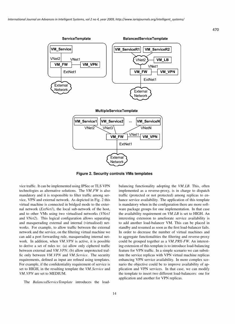
470


Figure 2. Security controls VMs templates

vice traffic. It can be implemented using IPSec or TLS VPNtechnologies as alternative solutions. The VM FW is alsomandatory and it is responsible to filter traffic among ser-vice, VPN and external network. As depicted in Fig. 2 thisvirtual machine is connected in bridged mode to the exter-nal network (ExtNet1), the local sub-network of the host,and to other VMs using two virtualised networks (VNet1and VNet2). This logical configuration allows separatingand masquerading external and internal (virtualised) net-works. For example, to allow traffic between the externalnetwork and the service, on the filtering virtual machine wecan add a port forwarding rule, masquerading internal net-work. In addition, when VM VPN is active, it is possibleto derive a set of rules to: (a) allow only ciphered trafficbetween external and VM VPN; (b) allow unprotected traf-fic only between VM VPN and VM Service. The securityrequirements, defined as input are refined using templates.For example, if the confidentiality requirement of service isset to HIGH, in the resulting template the VM Service andVM VPN are set to MEDIUM.

The BalancedServiceTemplate introduces the load-

balancing functionality adopting the VM LB. This, oftenimplemented as a reverse-proxy, is in charge to dispatchtraffic (protected or not protected) among replicas to en-hance service availability. The application of this templateis mandatory when in the configuration there are more soft-ware package groups for one implementation. In that casethe availability requirement on VM LB is set to HIGH. Aninteresting extension to ameliorate service availability isto add another load-balancer VM. This can be placed instandby and resumed as soon as the first load-balancer fails.In order to decrease the number of virtual machines andto aggregate functionalities the filtering and reverse-proxycould be grouped together as a VM PRX-FW. An interest-ing extension of this template is to introduce load-balancingfeature for VPN traffic. In a simple scenario we can substi-tute the service replicas with VPN virtual machine replicasenhancing VPN service availability. In more complex sce-nario the objective could be to improve availability of ap-plication and VPN services. In that case, we can modifythe template to insert two different load-balancers: one forapplication and another for VPN replicas.

14

471


Finally the last template MultipleServiceTemplate is suit-able to displace different service virtual machines on thesame physical host. In this configuration each service isdirectly linked to the VM FW using a virtual sub-networkwith specific network address and the VPN gateway isshared to different services. However it is possible config-ure the virtual machines to belong to the same sub-network.Grouping together the service VMs allows optimizing theirallocation enhancing general performance introducing a se-curity drawback. In fact, each service is protected usingthe same VPN channel and if the VPN is compromised, alltraffic could be jeopardized. To reduce the related risk thetemplate could be modified to support different VPN gate-ways. Practically we can displace a shared VPN gatewayfor non critical service and a specific VPN VM for eachcritical service.

4.2.2 Security controls transformations

Once the tool selects the set of templates to adopt, it per-forms a set of transformations to refine the provided in-formation. A transformation T is an operation that takesas input a set of services, a template and security require-ments and produces a set of alternative configurations. Asubset of security controls transformations is depicted inFig. 3. A configuration is expressed using an XML basedlanguage and contains: (a) the VM components; (b) the vir-tualised and physical network description; (c) the policiesto enforce. The VM components and the virtual networklinks are derived from the set of services and template, thenthe virtual and physical network configuration are computedconsequently. The firewall virtual machine is directly con-nected using a bridge to the physical network. The relatedexternal IP should be assigned accordingly to physical hostsubnet evaluating network description. The algorithm, aftera network analysis, proposes to the administrator a set ofavailable IPs. For each virtual links the algorithm computesthe network configuration for each virtual machine. In prac-tice it selects the addresses range from a table that containsthe allocations for private networks (populated consideringthe [1]) and generates other network information (gateway,DNS). Finally, the tool generates the related policies for theprovided solution. This process is composed by two steps:(1) generation of channel protection policies; (2) genera-tion of filtering policies. Considering the selected securitytechnology and the service description, the algorithm gen-erates the related properties for each virtual machine relatedto a protected communication. For example, if the selectedtechnology is HTTP over TLS, the TLS properties (e.g. ci-pher suite, server authentication or mutual authentication,etc. ) are attached to the service virtual machine componentconfiguration. In similar manner, when the tool selects TLSVPN or IPSec, the algorithm attaches the related proper-

ties to the VPN component. Finally the algorithm evaluatesthe components security properties and virtual network con-figuration generates the filtering policies. In practice, thefirewall VM is configured to forward traffic between exter-nal world and internal services according to security prop-erties. For example, if the internal service is protected usingHTTP over TLS, the firewall policy forwards only HTTPStraffic between external and internal networks. To clarify

Listing 7. Network configuration and policiesfor (a)

<VM id=’VM_Service’><network-interface value=’eth0’><addr type=’IPv4’ value=’10.10.10.2’ /><netmask value=’255.255.255.0’ /><gateway value=’10.10.10.1’ /><dns value=’ask to admin’ />

</network-interface></VM>

<VM id=’VM_FW’>//bridged interface<network-interface value=’eth0’><addr type=’IPv4’ value=’ask to admin’ /><netmask value=’ask to admin’ /><gateway value=’ask to admin’ /><dns value=’ask to admin’ />

</network-interface>//VNet1<network-interface value=’eth1’><addr type=’IPv4’ value=’10.10.10.1’ /><netmask value=’255.255.255.0’ /><gateway value=’ask to admin’ /><dns value=’ask to admin’ />

</network-interface><policies><filtering-policy id=’1’><type=’forwarding’ /><src ip=’*’ proto=’tcp’ port=’80’ /><dst ip=’10.10.10.2’ proto=’tcp’ port=’80’ /><action value=’allow’ />

</filtering-policy></policies>

</VM>

the security controls refinement we discuss the transforma-tions of Fig. 3. The most simple transformation is iden-tified by (a) and generates a configuration that contains aservice and a firewall virtual machines. The tool (1) de-fines the properties of the virtual network that links serviceto the firewall; (2) generates a port forwarding policy to al-low external traffic reaching internal service using specificprotocol and port. The algorithm analyses the table of pri-vate addresses and provides the network configurations forthe virtual machines shown in listing 7. For example, letus consider that the service is a web server that uses HTTPprotocol on port 80: the firewall (VM FW) is configured toforward traffic from external network to the internal serviceas described in listing 7.

The (b) example demonstrates service load-balancing.In this case the tool generates network configurations for:(1) the sub-network VNet2 that contains the load-balancer

15

472


s1

External

Network

T(s1, ServiceTemplate, secReq)

VM_FW

VM_s1

External

Network

SecReq:

CIA=(LOW,

LOW, LOW)

s1R1

External

Network

SecReq:

CIA=(HIGH,

HIGH, HIGH)

T((s1R1,s2R2), BalancedServiceTemplate,

secReq)

s1R2

VM_FW

External

Network

ExtNet1

VM_VPN

s1

External

Network

SecReq:

CIA=(HIGH,

HIGH, LOW)

s2

VM_FW

VM_s1

VM_VPN

External

Network

VM_s2

T((s1, s2), MultipleServiceTemplate,

secReq)

T((s1, s2), ServiceTemplate,

secReq)

VM_FWs1

VM_s1 VM_VPNs1

VM_FWs2

VM_s2

VM_VPNs2

External

Network

(a) (b)

(c)

VM_s1R1

VM_LB

VM_s1R2

VNet2VNet1

ExtNet1VNet1

ExtNet1

VNet1

VNet2 VNet3

ExtNet1

VNet1s1VNet2s1

VNet1s2

VNet2s2

(c1) (c2)

Figure 3. Security controls transformations

(VM LB) and the replicas (VM s1R1 and VM s1R2); (2)the sub-network VNet1 that contains the VPN gateway(VM VPN). The virtual firewall (VM FW) policies are: (1)port forwarding for load-balanced services; (2) port for-warding for VPN service (if the gateway is based on TLSVPN technology). In addition, the tool configures theVM LB to balance traffic among replicas and the VM VPNto protect communications. The load-balancer configura-

tion depends on mechanism selected to implement its func-tionality. The VPN gateway, often implemented as TLSVPN (for flexibility purposes), can be configured as clientor server. For example, it is often configured as server onthe service side and in client mode on external clients (any-to-one interaction model). In other cases, VPN gatewayscould be configured as one-to-one, i.e. to tunnel traffic be-tween two different services or any-to-any, i.e. to tunnel

16

473


Listing 8. VPN and balancer network configu-ration and policies for (b)

<VM id=’VM_VPN’><network-interface value=’eth0’><addr type=’IPv4’ value=’10.10.10.2’ /><netmask value=’255.255.255.0’ /><gateway value=’10.10.10.1’ /> <dns value=’ask to admin’ />

</network-interface><vpn-network-conf><vpn-pool type=’IPv4’ lowValue=’10.10.10.5’

highValue=’10.10.10.10’/><vpn-service-addr type=’IPv4’ value=’10.10.10.2’ /><vpn-service-interface type=’tap’ value=’tap0’/><vpn-service-protocol type=’tcp’ port=’1194’/>

</vpn-network-conf></VM><VM id=’VM_LB’><network-interface value=’eth0’><addr type=’IPv4’ value=’10.10.20.2’ /><netmask value=’255.255.255.0’ /><gateway value=’10.10.20.1’ /> <dns value=’ask to admin’ />

</network-interface><balancer-conf><balancer id=’balancer-VM_LB’><addr type=’IPv4’ value=’10.10.20.2’ /><proto type=’tcp’ port=’80’ />

</balancer><replicas><replica id=’replica-VM_s1R1’><addr type=’IPv4’ value=’10.10.20.3’ /><proto type=’tcp’ port=’80’ />

</replica><replica id=’replica-VM_s1R2’><addr type=’IPv4’ value=’10.10.20.4’ /><proto type=’tcp’ port=’80’ />

</replica></replicas>

</balancer-conf><balancer-policies><balancer-policy id=’1’><balancer-fronted value=’balancer-VM_LB’/><balancer-replica value=’replica-VM_s1R1’/><balancer-replica value=’replica-VM_s1R2’/>

</balancer-policy></balancer-policies>

</VM><VM id=’VM_s1R1’><network-interface value=’eth0’><addr type=’IPv4’ value=’10.10.20.3’ /><netmask value=’255.255.255.0’ /><gateway value=’10.10.20.1’ /><dns value=’ask to admin’ />

</network-interface></VM><VM id=’VM_s1R2’><network-interface value=’eth0’><addr type=’IPv4’ value=’10.10.20.4’ /><netmask value=’255.255.255.0’ /><gateway value=’10.10.20.1’ /><dns value=’ask to admin’ />

</network-interface></VM>

traffic among different services. In listings 8, 9 we proposea configuration to balance VM s1R1 and VM s1R2 replicas.In this case, we adopt the TLS VPN approach and the listing8 contains useful information for VM VPN configuration.First of all, the definition of the network addresses which

belong to the VPN and assigned to clients, in that case, thetool allocates 5 IPs from 10.10.10.5 to 10.10.10.10. In ad-dition, the tool generates, using the specific TLS VPN tem-plate, the virtual interface (tap0) and the protocol and portof the VPN service (tcp/1194). To allow external clients ac-cessing the internal services (VM s1R1 and VM s1R2) theymust join to the VPN. For that purpose, the virtualised fire-wall is configured to forward ciphered traffic (using TCPprotocol) to the virtual host 10.10.10.2 on port 1194. Theload balancer configuration is quite simple and contains thedescription of adopted replicas and a set of policies to bal-ance traffic. In practice for each replica the tool defines anIP address that belongs to the VNet2 and adds VM s1R1 andVM s1R2 as members of balancing pool.

Listing 9. Firewall network configuration andpolicies for (c)

<VM id=’VM_FW’>//bridged interface<network-interface value=’eth0’><addr type=’IPv4’ value=’ask to admin’ /><netmask value=’ask to admin’ /><gateway value=’ask to admin’ /><dns value=’ask to admin’ />



</network-interface><policies>//allow access to VPN<filtering-policy id=’1’><type=’forwarding’ /><src ip=’*’ proto=’tcp’ port=’1194’ /><dst ip=’10.10.10.2’ proto=’tcp’ port=’1194’ /><action value=’allow’ />

</filtering-policy>//allow access to balancer<filtering-policy id=’2’><type=’forwarding’ /><src ip=’10.10.10.*’ proto=’tcp’ port=’80’ /><dst ip=’10.10.20.2’ proto=’tcp’ port=’80’ /><action value=’allow’ />

</filtering-policy></policies>

</VM>

The last example (Listing 9) describes the alternative so-lutions (c1 and c2) to configure a set that aggregates two ormore services. The major difference between the providedsolutions is that in (c1) each service is protected by a ded-icated firewall and VPN gateway, on the contrary, the (c2)adopts shared firewall and VPN virtual machines. The dif-ferent approaches have pros and cons. The dedicated fire-

17

474


wall and VPN allow protecting the services in more finegrained way. For example, if a VPN channel is compro-mised, the other services are not involved. On the contrary,if we adopt a shared VPN gateway, in case of attacks, eachservice could be compromised. However the use of sharedresources enhances the entire system performance. In addi-tion, the configuration of dedicated firewall and VPN, oftenrequires assigning an external IP address for each firewall(VM FWs1 and VM FWs2) to correctly perform the portforwarding. Consider for example that VM s1 and VM s2are web servers hosting s1 and s2 applications and eachone communicates with external world using tcp protocolon port 80. In this situation we need to assign an external IPaddress for each firewall to distinguish s1 and s2 requests.

5 Virtual machines generation and manage-ment

Once the VM configurations are generated, it is neces-sary create and configure the related VMs to implement asolution. This goal requires the creation of the software en-vironment that hosts the services, the configuration of net-works, services, policies and the deployment of the VM to aphysical host. In addition, to react on fault events, it is alsoimportant monitor VM services, manage startup, shutdownand migration of the virtual machines.

5.1 Building software environment andspecific configurations

Several approaches could be followed to build the soft-ware environment, for example it is possible create manu-ally a base system template, building a VM from a com-mon GNU/Linux distribution. Then, the base system tem-plate could be modified in automatic way, generating a setof specific templates, adding the required software pack-ages to implement services. For example, the base sys-tem could be transformed into a VPN VM template addingIPSec or OpenVPN software packages. Similarly addingthe Apache Tomcat package we can implement a web serverVM template. The next step requires translating the ser-vices, network configuration and policies from a technologyspecific and device/service independent language (previousdescribed models) to the device/service specific language(e.g. network configuration for a GNU/Linux system, rulesfor a netfilter firewall). This task can be performed usinga set of adapters, one for each device/service category. Forexample, an adapter for VPN should be able to translate anIPSec configuration into the racoon specific language and aTLS VPN into the OpenVPN language. Similarly, for filter-ing, the adapter should translate the device/service indepen-dent configuration into a set of netfilter or PF (OpenBSD

Packet Filter) rules. The adapter output is a device/servicespecific configuration that must be deployed into the VM.

5.2 Deploying and Managing VMs

Finally, the configured VMs should be deployed into thephysical machine that will host the services. This task re-quires to: (1) identify which physical machine are able tohost the VMs; (2) define a set of mechanisms to transferthe VMs to physical hosts. Parsing the system descriptionmodel allow to identify which physical hosts support vir-tualisation and which are their performance. This informa-tion is useful to know how many virtual machines can bedeployed on a particular host. The deployment process, orin other words the task that transfers the VM to a physi-cal host, is quite simple but it depends on the virtualisa-tion technology adopted (e.g. Xen, KVM, VMware, etc. ).On the contrary the VM managing tasks (startup, shutdown,migration, network and disk management) are not simple toaddress. To handle these tasks and reducing the problemcomplexity a possible solution is to adopt a toolkit, like lib-virt [15], able to deal with different virtualisation technolo-gies, hiding details. The libvirt toolkit offers a set of API tointeract with the virtualisation capabilities of physical hoststo deploy and manage VMs.

5.3 Our approach

In this section we describe our approach to generate andmanage the virtual machines accordingly to the previous de-fined models.

5.3.1 Architecture layers

To perform the tasks described before we introduce in ourarchitecture three different layers: VM software, VM config-uration, VM management. The VM software layer containsthe activities to build a specific VM template like VM FW,VM VPN, VM LB and VM for specific services, for exam-ple to host Apache Tomcat web application. More prac-tically we start from a common GNU/Linux distribution,built manually, to derive automatically a set of predefinedtemplates, adding the required packages, e.g. OpenVPN forVM VPN. To perform this process automatically we adopta tool (ubuntu-vm-builder [27]) able to add new softwarepackages to a virtual machine. The predefined templatescould be generated only once, when the tool is run for thefirst time. On the contrary, a specific template that hostsa particular service must be generated when needed. Thebuild process is performed on a particular physical host,the builder machine that is also used to deploy and manageVMs. The VM configuration layer performs the followingtasks: (1) VM internal network configuration; (2) service

18

475


configuration; (3) policy configuration; (4) VM configura-tion. The VM internal network configuration is generatedaccordingly to the security controls transformation, startingfrom network configuration and policies model, defined be-fore. The information is translated using a specific adapterthat transforms the model to a specific network configura-tion language. For example, considering the listing 7 andsuppose that the VM is implemented using an Ubuntu Linuxoperating system, each VM network configuration is trans-lated into ’/etc/network/interfaces’ language. For bridginginterfaces, the tool asks to admin the IP address that shouldbe defined accordingly to physical host and external net-work. The service configuration, for example an ApacheTomcat web application, is translated using a specific tem-plate and a service dependant adapter. The policies, simi-larly to network configuration are translated from networkconfiguration and policies model to a specific security con-trol language, e.g. netfilter, using a specific adapter. Finallyit is necessary to build the configuration of the virtual ma-chine as XML model. To perform this step the tool takes asinputs (a) the VM template generated before (e.g. VM FW);(b) network configuration and policies model. Consideringthe listing 10, the template is used to define every propertiesof the XML model except for the network interface tags,that are generated using network configuration and policymodel. In addition, this model is used to create the virtualnetwork properties, as shown for VNet1 in listing 11. Thespecific configurations, except for virtual network proper-ties, derived from previous tasks, are deployed into the VM.More practically, the VM disk is mounted on local file sys-tem of the builder machine, and specific configuration arecopied accordingly. On the contrary the virtual networkproperties are used in the next step to configure the virtu-alisation environment.

The VM management layer is able to setup the virtuali-sation environment, deploy, migrate, start and stop a virtualmachine. In order to create and deploy a VM on the physi-cal host, the first activity is setup the virtualisation environ-ment. In practice, our tool, using the libvirt-java API, cre-ates the network environment on the remote host, accord-ingly to the network properties described in listing 11. Inthe next step, the tool takes as input the VM configurationmodel of 10 and using the API creates the new domain onremote physical host. Finally, the last step copies the VMdisk on the remote host, and the VM is ready to start.

6 Conclusion

We have analysed how the best practices for service andnetwork dependability change when exploiting modern vir-tualisation technologies. Based on the results of this study,we have updated the process and tools we had developedfor semi-automatic dependability planning of information

Listing 10. libvirt VM configuration model<domain type=’kvm’><name>vm-fw1</name><uuid>0cc4736f-2568-241d-c610-2e7ba90002f5</uuid><memory>262144</memory><currentMemory>262144</currentMemory><vcpu>1</vcpu><os><type arch=’i686’ machine=’pc-0.11’>hvm</type><boot dev=’hd’/>

</os><features><acpi/><apic/><pae/>

</features><clock offset=’utc’/><on_poweroff>destroy</on_poweroff><on_reboot>restart</on_reboot><on_crash>restart</on_crash><devices><emulator>/usr/bin/kvm</emulator><disk type=’file’ device=’disk’><source file=’/home/vm-deployment/vm-fw1-disk.img’

/><target dev=’hda’ bus=’ide’/>

</disk><disk type=’file’ device=’cdrom’><target dev=’hdc’ bus=’ide’/><readonly/>

</disk><interface type=’network’><mac address=’54:52:00:60:ef:e5’/><source network=’VNet1’/>

</interface><interface type=’bridge’><mac address=’54:52:00:04:3b:c0’/><source bridge=’br0’/>

</interface><serial type=’pty’><target port=’0’/>

</serial><console type=’pty’><target port=’0’/>

</console><input type=’mouse’ bus=’ps2’/><graphics type=’vnc’ port=’-1’ autoport=’yes’ keymap=

’it’/><video><model type=’cirrus’ vram=’9216’ heads=’1’/>

</video></devices>

</domain>

Listing 11. libvirt virtual network propertiesfor VNet1

<network><name>VNet1</name><uuid>3e3fce45-4f53-4fa7-bb32-11f34168b82b</uuid><bridge name=’virbr1’ stp=’on’ forwardDelay=’0’ /><ip address="10.10.10.254" netmask="255.255.255.0"><dhcp><range start="10.10.10.100" end="10.10.10.200" /><host mac="54:52:00:60:ef:e5" name="VM_FW" ip="

10.10.10.1" /></dhcp>

</ip></network>

systems.

19

476


In particular, this paper has detailed the algorithms thatour tools exploit to automatically compute allocation andreaction plans for virtualised information systems. Each al-gorithm is defined in terms of the relevant modelling on-tology and the pool of transformation rules working on thisontology. The actual implementation exploits XML repre-sentations and transformation languages. We have also de-veloped prototype integration of our tools with popular vir-tual machine management software, which is an essentialstep towards automatic deployment of the generated plans.

During the selection of the relevant configuration strate-gies, we have focused on the point of view of the virtualdata center customer: our approach can, and should be, ex-tended taking in further consideration the point of view ofthe hosting provider, which may partially conflict with thecustomer’s one.

Acknowledgment

This work was developed in the framework of IST-026600 DESEREC, “Dependability and Security by En-hanced Reconfigurability”, an Integrated Project partiallyfunded by the E.C. under the Framework Program 6, ISTpriority.

References

[1] Network Working Group, Address Allocation for Private In-ternets. IETF RFC 1918, February 1996.

[2] W3C Consortium, Web Services Choreography DescriptionLanguage. http://www.w3.org/TR/ws-cdl-10/,2005.

[3] POSITIF Consortium, The POSITIF System DescriptionLanguage (P-SDL). http://www.positif.org/,2007.

[4] National Vulnerability Database. http://nvd.nist.gov/, 2008.

[5] Common Vulnerability Scoring System. http://www.first.org/cvss/, 2009.

[6] M. D. Aime, P. C. Pomi, and M. Vallini. Policy-drivensystem configuration for dependability. Emerging SecurityInformation, Systems, and Technologies, The InternationalConference on, 0:420–425, 2008.

[7] M. D. Aime, P. C. Pomi, and M. Vallini. Planning depend-ability of virtualised networks. Dependability, InternationalConference on, 0:46–51, 2009.

[8] Amazon. Amazon Elastic Compute Cloud (Amazon EC2).http://aws.amazon.com/ec2/.

[9] P. Barham, B. Dragovic, K. Fraser, S. Hand, T. Harris,A. Ho, R. Neugebauer, I. Pratt, and A. Warfield. Xen andthe art of virtualization. In SOSP ’03: Proceedings of thenineteenth ACM symposium on Operating systems princi-ples, pages 164–177, 2003.

[10] N. Damianou, N. Dulay, E. C. Lupu, and M. Sloman. Pon-der: a language for specifying security and management

policies for distributed systems. Imperial College ResearchReport DoC 2000/1, 2000.

[11] T. Eilam, M. Kalantar, A. Konstantinou, G. Pacifici, J. Per-shing, and A. Agrawal. Managing the configuration com-plexity of distributed applications in internet data centers.Communications Magazine, IEEE, 44(3):166–177, March2006.

[12] P. Giorgini, F. Massacci, J. Mylopoulos, and N. Zannone.Requirements engineering meets trust management - model,methodology, and reasoning. In In Proc. of iTrust ’04, LNCS2995, pages 176–190. Springer-Verlag, 2004.

[13] M. Israel, J. Borgel, and A. Cotton. Heuristics to performmolecular decomposition of large mission-critical informa-tion systems. In SECURWARE ’08: Proceedings of the 2008Second International Conference on Emerging Security In-formation, Systems and Technologies, pages 338–343, 2008.

[14] L. Lamport, R. Shostak, and M. Pease. The byzantine gen-erals problem. ACM Transactions on Programming Lan-guages and Systems, 4:382–401, 1982.

[15] libvirt. http://libvirt.org/.[16] A. Menon, A. L. Cox, and W. Zwaenepoel. Optimizing Net-

work Virtualization in Xen. Proceedings of the USENIXAnnual Technical Conference, 2006.

[17] Microsoft Corporation. Azure Service Platform. http://www.microsoft.com/azure/.

[18] D. M. Nicol, W. H. Sanders, and K. S. Trivedi. Model-basedevaluation: From dependability to security. IEEE Trans-actions on Dependable and Secure Computing, 1(1):48–65,2004.

[19] J. Oberheide, E. Cooke, and F. Jahanian. Empirical exploita-tion of live virtual machine migration. In In Proceedings ofthe BlackHat DC convention, 2008.

[20] E. Rescorla, A. Cain, and B. Korver. SSLACC: A ClusteredSSL Accelerator. In Proceedings of the 11th USENIX Secu-rity Symposium, pages 229–246, Berkeley, CA, USA, 2002.USENIX Association.

[21] J. Salowey, H. Zhou, P. Eronen, and H. Tschofenig. Trans-port Layer Security (TLS) Session Resumption withoutServer-Side State. IETF RFC 5077, January 2008.

[22] F. Satoh, Y. Nakamura, N. K. Mukhi, M. Tatsubori, andK. Ono. Methodology and tools for end-to-end soa secu-rity configurations. In SERVICES ’08: Proceedings of the2008 IEEE Congress on Services - Part I, pages 307–314,Washington, DC, USA, 2008. IEEE Computer Society.

[23] J. Strassner. Policy-Based Network Management: Solutionsfor the Next Generation (The Morgan Kaufmann Series inNetworking). Morgan Kaufmann Publishers Inc., San Fran-cisco, CA, USA, 2003.

[24] The DMTF Technical Committee. The Common In-formation Model (CIM). http://www.dmtf.org/standards/cim, 2008.

[25] Trusted Computing Group. https://www.trustedcomputinggroup.org, 2009.

[26] Ubuntu. Ubuntu Enterprise Cloud. http://www.ubuntu.com/cloud/private.

[27] Ubuntu. ubuntu-vm-builder. https://help.ubuntu.com/8.04/serverguide/C/ubuntu-vm-builder.html.

[28] VMware. http://www.vmware.com.

20

477

International Journal on Advances in Intelligent Systems, vol 2 no 4, year 2009, http://www.iariajournals.org/intelligent_systems/1

Model Transformations Given Policy Modificationsin Autonomic Management

Raphael M. Bahati and Michael A. BauerDepartment of Computer Science

The University of Western Ontario, London, ON N6A 5B7, CANADAEmail: {rbahati;bauer}@csd.uwo.ca

Abstract—This paper presents an approach for adapting amodel learned from the use of an active set of policies torun-time policy modifications. The work leverages our mostresent efforts utilizing Reinforcement Learning methodologies tofacilitate dynamic use of policies within autonomic computing.The use of policies in this context offers significant benefits toautonomic systems in that it allows systems to determine how toeffectively meet the desired, and at times seemingly conflicting,objectives under dynamically changing conditions. Contrary toother approaches that make use of some form of learningto model performance management, our approach enables themodel learnt from the use of an active set of policies to be reusedonce those policies change. Since the learning mechanisms aremodelled from the structure of the policies, policy modificationscan be mapped onto the learnt model. Our analysis of thepolicy modifications suggest that most of the learned model couldbe reused, potentially accelerating the learning process. In thispaper, we provide formal definitions on the different kinds ofpolicy modifications that might occur as well as elaborate, withdetailed examples, on how such modifications could impact thecurrently learned model.

Index Terms—Model Transformation, Model Adaptation, Re-inforcement Learning, Autonomic Management, Policy-basedManagement.

I. INTRODUCTION

Policy-based management has been proposed as a wayin which the behavior of systems and applications can beadjusted at run-time rather than through re-engineering [1].The concept of policy-based management has been adoptedby standard bodies such as the (Internet Engineering TaskForce (IETF) [2], the Distributed Management Task Force(DMTF) [3], and the Object Management Group (OMG) [4].Policy-based management has also attracted significant interestfrom a wide variety of efforts, ranging from academia [5] toindustry [6], which have resulted in a great deal of diversityin terms of what policies are and how they should be used.

It is often common that policies are used to express requiredor desired behavior of systems and applications. In the contextof autonomic computing, for example, policies can be inputto or embedded within the autonomic management elementsof the system to provide the kinds of directives which anautonomic manager could make use of in order to meetoperational requirements. Thus, through the modifications ofthe policies driving autonomic management, the behavior ofsystems could be dynamically adjusted. Such directives couldcome from the users of such systems or other autonomicmanagement elements within the computing environment.

While the use of policies has been the subject of con-siderable research focus, very little work has been done onevaluating the effectiveness of the policies when in use todetermine whether the performance objectives are, in fact,being met. More often than not, policy use within autonomiccomputing has typically focused on the specification and use“as is” within systems. It is often assumed, for example,that once the policies are specified, the system would behaveas expected. Consequently, many of these approaches fail torecognize the stochastic, dynamic, and heterogeneous natureof today’s systems which necessitates the need for autonomicsystems to adapt not only to how they use policies, butalso to run-time policy modifications. This is essential inorder for systems to cope with not only changes to theconfiguration of the managed environment, but also changesto the perceived quality of services, something that is oftentime-, user-dependent, and application-specific.

To this end, we have proposed an adaptive policy-drivenautonomic management framework highlighting two key con-tributions in the use of policies within autonomic computing:(1) The ability to evaluate, through model-learning, the effec-tiveness of the enabled policies based on past experience fromtheir use which, in turn, provide guidance to the autonomicsystem on how to effectively use the policies [7]. (2) Theability to adapt the model learned from the use of policiesto run-time policy modifications, essentially allowing most ofthe learned model to be reused in the new environment [8].The focus of this work is on the second of these approaches.It expands on the strategies we initially proposed in [8] byformally describing the types of changes to a set of policiesthat could occur and how we map such changes to modeltransformations. This is done within the context of the adaptivepolicy-driven autonomic management framework in [9].

The rest of the paper is organized as follows. We beginwith an overview of how we model learning in Section II,summarizing some of the key definitions we make use of inthis paper. We then present our approach to model adaptationin Section III. The section begins with formal definitions ofthe types of changes that might occur to a set of policies, andthen describe how such modifications are mapped to specificcases of model transformations. We summarize the results ofthe experiments in Section IV, describe some related work inSection V, and conclude in Section VI.

478


II. LEARNING BY REINFORCEMENT

This section summarizes key definitions outlining our ap-proach to modelling Reinforcement Learning [10] in the con-text of policy-driven autonomic management. A more detailedaccount can be found in [7].

Definition 1: An expectation policy is defined by the tuplepi = 〈C,A〉 where:

• C is conjunctive conditions associated with policy pi

with each condition, cj ∈ C, defined by the tuple cj =〈ID, metricName, operator, Γ〉, where ID is aunique identification for the condition; metricName isthe name of the metric associated with the condition;operator is the relational operator associated with thecondition; and Γ is the threshold of the condition.

• A is a set of actions associated with policy pi witheach action, aj ∈ A, defined by the tuple aj = 〈ID,function, parameters, τ〉, where ID is a uniqueidentification for the action; function is the name ofthe function that should be executed; parameters isa set of function parameters; and τ is a set of testsassociated with the action.

A policy-driven autonomic management system is likely toconsist of multiple expectation policies, a subset of which maybe active (or enabled) at any given time, which brings us toour next definition.

Definition 2: Suppose that PA denotes a set of all expecta-tion policies such that pi ∈ PA where pi = 〈C,A〉. Let P bea subset of expectation policies an autonomic manager uses tomake management decisions; i.e., P ⊆ PA. A policy systemcorresponding to P is defined by the tuple PS = 〈P,WC〉where:

• WC = 〈ci, ωi〉 associates each policy condition, ci, with ametric weight, ωi, such that, for all ci ∈ pm and cj ∈ pn,ωi = ωj if ci.metricName = cj .metricName.

Essentially, a policy system is the set of active policies whereeach condition occurring in some policy has an associatedweight. The metrics weights, which are specified manually inour current implementation, provide a way of distinguishingpolicy conditions based on the significance of violating aparticular metric. In essence, WC provides a way of biasinghow the autonomic system responds to quality of serviceviolations. These definitions provide the fundamental structurethat is used to build our reinforcement learning model.

A. System States

To model system’s dynamics from the use of an activeset of policies, we make use of a mapping between theenabled expectation policies and the managed system’s stateswhose structure is derived from the metrics associated withthe enabled policy conditions.

Definition 3: A policy system PS = 〈P,WC〉 derives a setof system metrics, mi ∈M , such that, for each pj = 〈Cj , Aj〉where pj ∈ P , M =

⋃ci∈Cj

{ci.metricName}.

The set M is the set of all metrics occurring in any of theactive policies. For each metric in this set, there are a finite

number of threshold values to which the metric is compared;there can be ordered to form regions:

Definition 4: A policy system PS = 〈P,WC〉 with metricsset M derives a set of metric regions, rmi ∈ MP

R , for eachmetric mi ∈M , whose structure is defined by the tuple rmi =〈αmi , σmi〉, where:

• αmi= 〈ID, metricName, ω〉 corresponds to a unique

metric from among the metrics of the conditions of thepolicies in P ; such that, metricName is the name ofthe metric and ω is the weight of the condition (seeDefinition 2) associated with metric mi.

• σmi = {Γ1,Γ2, . . . ,Γk} is a set of thresholds from theconditions associated with metric mi such that, Γi <Γj if i < j. As such, σmi derives a set of metricregions which map the observed metric measurementonto appropriate localities (i.e., intervals) as defined bythe thresholds of the policy conditions associated withmetric mi, such that Rmi = {R1

mi, R2

mi, . . . , Rk+1

mi},

where R1mi

= (−∞,Γ1), R2mi

= (Γ1,Γ2), etc., andRk+1

mi= (Γk,∞).

To be precise, the actual boundaries of region Rjmi

aredetermined by the operators of the policy conditions asso-ciated with a given metric. For example, a system with twoconditions c1 = 〈ID,mi,>,Γ1〉 and c2 = 〈ID,mi,≥,Γ2〉such that σmi = 〈Γ1,Γ2〉 would yield three regions in ourapproach, namely: R1

mi= [−∞,Γ1), R2

mi= [Γ1,Γ2), and

R3mi

= [Γ2,∞]. Thus, a metric measurement of, say, Γ1 wouldfall into region R2

mi. This brings us to our next definition.

Definition 5: Given a set of metric-regions rmi∈ MP

R foreach metric mi ∈ M such that rmi = 〈αmi , σmi〉, whereσmi derives a set of metric regions Rj

mi∈ Rmi ; we define

a weighting function, f(Rjmi

)→ R, which assigns a numericvalue to the j-th region in Rmi such that, f(Rk

mi) > f(Rl

mi)

if k < l.An example of such a mapping, which we make use of in

our current implementation, is defined by Equation 1:

f(Rjmi

) = 100− (100

n− 1)(j − 1) (1)

where n is the total number of regions in Rmi . This functionassigns a numeric value between 100 and 0 for each metric’sregion in Rmi , starting from 100 for the most desirable regionand decrementing at equal intervals towards the opposite endof the spectrum, whose region is assigned a value of 0. Thisapproach guarantees that the highest value is assigned tothe most desirable region (i.e., the region corresponding tothe highest quality of service), assuming, of course, that theassumptions about the conditions of the expectation policieshold (see Definition 1). That is, smaller metric values are“more desirable” though, in general, this is not a necessaryrequirement of the weighting function. The idea is that, regionsof greater “desirability”, i.e., preferred quality of service, areassigned higher values. The key role of these regions is thatthey partition the space of values that a metric can take on withrespect to the thresholds in conditions involving that metric.We use these to define a state within our model.

Definition 6: A policy system PS = 〈P,WC〉 with metricsM and metrics-regions MP

R derives a set of system states

2

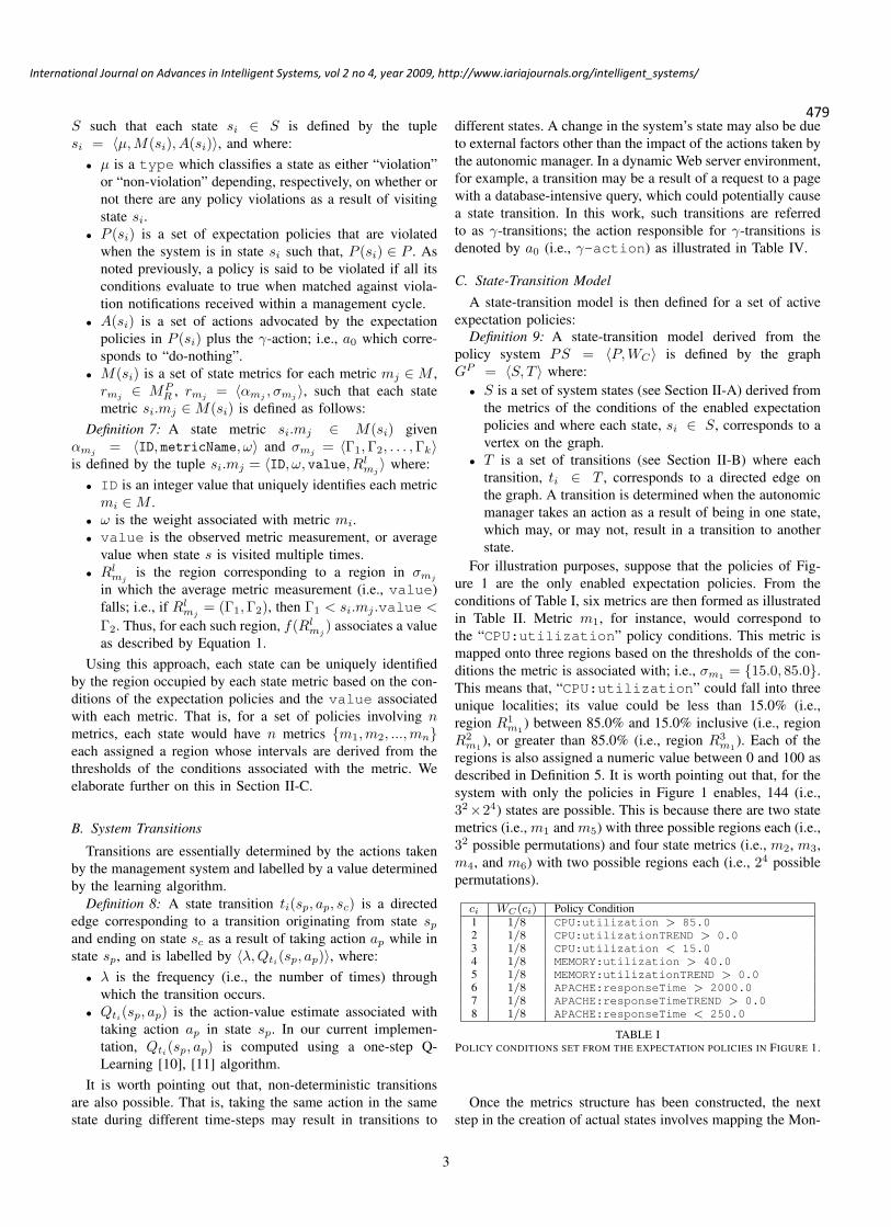
479


S such that each state si ∈ S is defined by the tuplesi = 〈µ,M(si), A(si)〉, and where:

• µ is a type which classifies a state as either “violation”or “non-violation” depending, respectively, on whether ornot there are any policy violations as a result of visitingstate si.

• P (si) is a set of expectation policies that are violatedwhen the system is in state si such that, P (si) ∈ P . Asnoted previously, a policy is said to be violated if all itsconditions evaluate to true when matched against viola-tion notifications received within a management cycle.

• A(si) is a set of actions advocated by the expectationpolicies in P (si) plus the γ-action; i.e., a0 which corre-sponds to “do-nothing”.

• M(si) is a set of state metrics for each metric mj ∈M ,rmj ∈ MP

R , rmj = 〈αmj , σmj 〉, such that each statemetric si.mj ∈M(si) is defined as follows:

Definition 7: A state metric si.mj ∈ M(si) givenαmj = 〈ID, metricName, ω〉 and σmj = 〈Γ1,Γ2, . . . ,Γk〉is defined by the tuple si.mj = 〈ID, ω, value, Rl

mj〉 where:

• ID is an integer value that uniquely identifies each metricmi ∈M .

• ω is the weight associated with metric mi.• value is the observed metric measurement, or average

value when state s is visited multiple times.• Rl

mjis the region corresponding to a region in σmj

in which the average metric measurement (i.e., value)falls; i.e., if Rl

mj= (Γ1,Γ2), then Γ1 < si.mj .value <

Γ2. Thus, for each such region, f(Rlmj

) associates a valueas described by Equation 1.

Using this approach, each state can be uniquely identifiedby the region occupied by each state metric based on the con-ditions of the expectation policies and the value associatedwith each metric. That is, for a set of policies involving nmetrics, each state would have n metrics {m1,m2, ...,mn}each assigned a region whose intervals are derived from thethresholds of the conditions associated with the metric. Weelaborate further on this in Section II-C.

B. System Transitions

Transitions are essentially determined by the actions takenby the management system and labelled by a value determinedby the learning algorithm.

Definition 8: A state transition ti(sp, ap, sc) is a directededge corresponding to a transition originating from state sp

and ending on state sc as a result of taking action ap while instate sp, and is labelled by 〈λ, Qti(sp, ap)〉, where:

• λ is the frequency (i.e., the number of times) throughwhich the transition occurs.

• Qti(sp, ap) is the action-value estimate associated withtaking action ap in state sp. In our current implemen-tation, Qti(sp, ap) is computed using a one-step Q-Learning [10], [11] algorithm.

It is worth pointing out that, non-deterministic transitionsare also possible. That is, taking the same action in the samestate during different time-steps may result in transitions to

different states. A change in the system’s state may also be dueto external factors other than the impact of the actions taken bythe autonomic manager. In a dynamic Web server environment,for example, a transition may be a result of a request to a pagewith a database-intensive query, which could potentially causea state transition. In this work, such transitions are referredto as γ-transitions; the action responsible for γ-transitions isdenoted by a0 (i.e., γ-action) as illustrated in Table IV.

C. State-Transition ModelA state-transition model is then defined for a set of active

expectation policies:Definition 9: A state-transition model derived from the

policy system PS = 〈P,WC〉 is defined by the graphGP = 〈S, T 〉 where:

• S is a set of system states (see Section II-A) derived fromthe metrics of the conditions of the enabled expectationpolicies and where each state, si ∈ S, corresponds to avertex on the graph.

• T is a set of transitions (see Section II-B) where eachtransition, ti ∈ T , corresponds to a directed edge onthe graph. A transition is determined when the autonomicmanager takes an action as a result of being in one state,which may, or may not, result in a transition to anotherstate.

For illustration purposes, suppose that the policies of Fig-ure 1 are the only enabled expectation policies. From theconditions of Table I, six metrics are then formed as illustratedin Table II. Metric m1, for instance, would correspond tothe “CPU:utilization” policy conditions. This metric ismapped onto three regions based on the thresholds of the con-ditions the metric is associated with; i.e., σm1 = {15.0, 85.0}.This means that, “CPU:utilization” could fall into threeunique localities; its value could be less than 15.0% (i.e.,region R1

m1) between 85.0% and 15.0% inclusive (i.e., region

R2m1

), or greater than 85.0% (i.e., region R3m1

). Each of theregions is also assigned a numeric value between 0 and 100 asdescribed in Definition 5. It is worth pointing out that, for thesystem with only the policies in Figure 1 enables, 144 (i.e.,32×24) states are possible. This is because there are two statemetrics (i.e., m1 and m5) with three possible regions each (i.e.,32 possible permutations) and four state metrics (i.e., m2, m3,m4, and m6) with two possible regions each (i.e., 24 possiblepermutations).

ci WC(ci) Policy Condition1 1/8 CPU:utilization > 85.02 1/8 CPU:utilizationTREND > 0.03 1/8 CPU:utilization < 15.04 1/8 MEMORY:utilization > 40.05 1/8 MEMORY:utilizationTREND > 0.06 1/8 APACHE:responseTime > 2000.07 1/8 APACHE:responseTimeTREND > 0.08 1/8 APACHE:responseTime < 250.0

TABLE IPOLICY CONDITIONS SET FROM THE EXPECTATION POLICIES IN FIGURE 1.

Once the metrics structure has been constructed, the nextstep in the creation of actual states involves mapping the Mon-

3

480


� �[ 1 ] e x p e c t a t i o n p o l i c y {CPUViola t ion (PDP , PEP)}

i f (CPU: u t i l i z a t i o n > 8 5 . 0 ) &(CPU: u t i l i z a t i o n T R E N D > 0 . 0 )

then{A d j u s t M a x C l i e n t s (−25)t e s t {newMaxClients > 49} |

Adjus tMaxKeepAl iveReques t s (−30)t e s t {newMaxKeepAliveRequests > 1} |

AdjustMaxBandwidth (−128)t e s t {newMaxBandwidth > 255}}

[ 2 ] e x p e c t a t i o n p o l i c y {RESPVio la t ion (PDP , PEP)}i f (APACHE: re sponseT ime > 2 0 0 0 . 0 ) &

(APACHE: responseTimeTREND > 0 . 0 )then{A d j u s t M a x C l i e n t s ( + 2 5 )

t e s t {newMaxClients < 151} &t e s t { I d l e W o r k e r s < 5} |

Adjus tMaxKeepAl iveReques t s (−30)t e s t {newMaxKeepAliveRequests > 1} |


[ 3 ] e x p e c t a t i o n p o l i c y {CPUandRESPViol . ( PDP , PEP)}i f (CPU: u t i l i z a t i o n > 8 5 . 0 ) &

(CPU: u t i l i z a t i o n T R E N D > 0 . 0 ) &(APACHE: re sponseT ime > 2 0 0 0 . 0 )

then{Adjus tMaxKeepAl iveReques t s (−30)t e s t {newMaxKeepAliveRequests > 1} |


[ 4 ] e x p e c t a t i o n p o l i c y {MEMORYViolation (PDP , PEP)}i f (MEMORY: u t i l i z a t i o n > 4 0 . 0 ) &

(MEMORY: u t i l i z a t i o n T R E N D > 0 . 0 )then{A d j u s t M a x C l i e n t s (−25)

t e s t {newMaxClients > 49}}[ 5 ] e x p e c t a t i o n p o l i c y {SERVERnormal (PDP , PEP)}

i f (CPU: u t i l i z a t i o n < 1 5 . 0 ) &(APACHE: re sponseT ime < 2 5 0 . 0 )

then{A d j u s t M a x C l i e n t s (−25)t e s t {newMaxClients > 49} &t e s t { I d l e W o r k e r s > 25} |

Adjus tMaxKeepAl iveReques t s ( + 3 0 )t e s t {newMaxKeepAliveRequests < 95}}� �

Fig. 1. Sample policy system where P = {p1, p2, p3, p4, p5}.

itor events collected during a single management interval ontoappropriate state metrics and regions. Suppose, for example,that during a single management interval, the managementsystem receives the events in Figure 2. By mapping the eventsusing the metrics structure in Table II, a new state is thencreated as illustrated in Table III; lets call it state s∗. For amanagement system with only the policies of Figure 1 enabled,being in state s∗ would mean the violation of policy p1; i.e..P (s∗) = {p1}. Thus, in addition to the action “a0 : γ-action” which corresponds to “doing nothing”, A(s∗) wouldconsist of a set of unique actions from the actions of thepolicies in P (s∗) as illustrated in Table IV.

CPU:utilization = 90.0CPU:utilizationTREND = 1.0MEMORY:utilization = 32.0MEMORY:utilizationTREND = -2.0APACHE:responseTime = 1500.0APACHE:responseTimeTREND = -1.0

Fig. 2. A set of Monitor events collected during a single management interval.

In the sections that follow, we describe our approach foradapting the state-transition model to run-time policy mod-ifications (denoted by 4[P ]) which we formally define inSection III-A.

III. ADAPTING TO POLICY CHANGES

Figure 3 describes our approach to model-adaptation. Theleft-part of the diagram (i.e., prior to 4[P ]) depicts theReinforcement Learning mechanisms described in Section II.whereby the agent learns the model of the environment basedon past experience in the use of an active set of policies, P .In this approach, the conditions of the policies define systemstates while the actions of the policies define possible causesof transitions between states. That is, at each time step, theagent takes action ai ∈ A(s) where A(s) is a set of actionsadvocated by the policies that are violated when the systemis in state s. This, in turn, causes a transition as depictedin the diagram. Thus, the model is continuously updatedbased on the experience garnered from the agent’s interactionwith its environment; i.e., based on the states and transitionsencountered. The right-part of the diagram (i.e., after 4[P ]occurs) depicts the mapping (using the transformation functionΨ) from the current system’s model (i.e., GP

n = 〈S, T 〉) to anew model (i.e., GP ′

n+1 = 〈S′, T ′〉), as a result of run-timemodification to the policies in P .

A. Types of Modifications

By run-time policy modifications, we mean any type ofmodification resulting in changes to the characteristics of thepolicies driving autonomic management. Since the structurespecific to the model of the environment is derived from thecharacteristics of the enabled policies (see Section II-A), anyrun-time changes to these characteristics could have possibleramifications on the learning process. This would likely de-pend on what kind of modification is done on the policies.

1) Adding/Removing a Policy: A policy modification couldinvolve adding a policy onto the policies in P ; i.e.,

Given:I) PS = 〈P,WC〉

II) p∗ = 〈C,A〉 where p∗ /∈ P :• C = {c1, c2, . . . , cx} : cx = 〈ID,metricName, operator, Γ〉

• A = {a1, a2, . . . , ay} : ay = 〈ID,function, parameters, τ〉

Then:1) PS′ = 〈P ′,WC〉 : P ′ ← P ∪ p∗

A policy modification could also involve removing anexisting policy from P ; i.e.,


II) p∗ = 〈C,A〉 where p∗ ∈ P :• C = {c1, c2, . . . , cx} : cx = 〈ID,metricName, operator, Γ〉

• A = {a1, a2, . . . , ay} : ay = 〈ID,function, parameters, τ〉

4

481


mi ck Policy Condition Rmi Rjmi

f(Rjmi

)

m1

3 CPU:utilization < 15.0 m1.value < 15.0 R1m1

10015.0 ≤ m1.value ≤ 85.0 R2

m150

1 CPU:utilization > 85.0 m1.value > 85.0 R3m1

0

m2m2.value ≤ 0.0 R1

m2100

2 CPU:utilizationTREND > 0.0 m2.value > 0.0 R2m2

0


m3100

4 MEMORY:utilization > 40.0 m3.value > 40.0 R2m3

0


m4100

5 MEMORY:utilizationTREND > 0.0 m4.value > 0.0 R2m4

0

m5

8 APACHE:responseTime < 250.0 m5.value < 250.0 R1m5

100250.0 ≤ m5.value ≤ 2000.0 R2

m550

6 APACHE:responseTime > 2000.0 m5.value > 2000.0 R3m5

0


m6100

7 APACHE:responseTimeTREND > 0.0 m6.value > 0.0 R2m6

0

TABLE IIMETRICS STRUCTURE DERIVED FROM THE EXPECTATION POLICIES OF FIGURE 1.

mi Metric Value Rmi Rjmi

f(Rjmi

)m1 CPU:utilization = 90.0 m1.value > 85.0 R3

m10

m2 CPU:utilizationTREND = 1.0 m2.value > 0.0 R2m2

0m3 MEMORY:utilization = 32.0 m3.value ≤ 40.0 R1

m3100

m4 MEMORY:utilizationTREND = -2.0 m4.value ≤ 0.0 R1m4

100m5 APACHE:responseTime = 1500.0 250.0 ≤ m5.value ≤ 2000.0 R2

m550

m6 APACHE:responseTimeTREND = -1.0 m6.value ≤ 0.0 R1m6

100

TABLE IIIs∗ - A STATE DERIVED FROM THE MONITOR EVENTS IN FIGURE 2 AND THE METRICS STRUCTURE OF TABLE II.

ai Q(s∗, ai) Policy Actionsa0 γ-actiona2 AdjustMaxClients(-25) test{newMaxClients > 49}a4 AdjustMaxKeepAliveRequests(-30) test{newMaxKeepAliveRequests > 1}a6 AdjustMaxBandwidth(-128) test{newMaxBandwidth > 255}

TABLE IVA(s∗) - A SET OF UNIQUE ACTIONS FROM THE ACTIONS OF THE POLICIES THAT ARE VIOLATED WHEN THE SYSTEM IS IN STATE s∗ .

Fig. 3. Adapting to run-time policy modifications.

Then:1) PS′ = 〈P ′,WC〉 : P ′ ← P |p∗

Since the impact of such modifications on the state-transition model would depend on what conditions and/oractions are affected as a result, adding/removing an entirepolicy can be modelled in the context of adding/removingindividual conditions and actions within policies.

On the one hand, adding policy p∗ = 〈C,A〉 into thepolicies in P can be modelled by the following sequence ofpolicy modifications: (i) Adding the policy without conditions

or actions; i.e., p∗ = 〈∅, ∅〉 (see below). (ii) Adding one con-dition at a time from the conditions in C (see Section III-A2).(iii) Adding one action at a time from the actions in A (seeSection III-A5).

Policy Modification - 4x[P]: Adding a policy without con-ditions or actions.


II) MPR = {r1, r2, . . . , rl} : ri = 〈αi, σi〉

III) p∗ = 〈∅, ∅〉 such that p∗ /∈ P

5

482


Then:1) PS′ = 〈P ′,WC〉 : P ′ ← P ∪ p∗2) M ′ ←M3) MP ′

R ←MPR

On the other hand, removing policy p∗ = 〈C,A〉 from thepolicies in P can be modelled by the following sequence ofpolicy modifications: (i) Removing one action at a time fromthe actions in A (see Section III-A6). (ii) Removing one con-dition at a time from the conditions in C (see Section III-A3).(iii) Removing the policy without conditions or actions; i.e.,p∗ = 〈∅, ∅〉 (see below).

Policy Modification - 4y[P]: Removing a policy withoutconditions or actions.



III) p∗ = 〈∅, ∅〉 such that p∗ ∈ P

Then:1) PS′ = 〈P ′,WC〉 : P ′ ← P |p∗2) M ′ ←M3) MP ′

R ←MPR

2) Adding a Policy Condition: Another type of policymodification could involve adding a condition into one of thepolicies in P .

Given:• PS = 〈P,WC〉• p∗ = 〈C,A〉 such that p∗ ∈ P• c∗ = 〈ID, metricName, operator, Γ〉

Then:1) PS′ = 〈P ′,WC〉 : p′∗ = 〈C ′, A〉 where C ′ ←

C ∪ c∗There are several ways in which adding a policy condition

could impact the system’s metrics structure (see Definition 4):In the first case, adding a policy condition may result in an

increase in the number of system metrics. This may be a resultof adding a policy condition whose metricName is not inany of the conditions of the policies in P .

Policy Modification - 41[P]: Adding a policy condition re-sulting in a new metric.



III) p∗ = 〈C,A〉 such that p∗ ∈ P where ∀ pi ∈ P ,c∗ /∈ pi

IV) c∗ = 〈ID, metricName, operator,Γ〉 such that m = c∗.metricName and wherem /∈M

V) rm /∈MPR : rm = 〈αm, σm〉 :

• αm = 〈ID, metricName, ω〉• σm = {Γ}


C ∪ c∗2) M ′ ←M ∪ m3) MP ′

R ←MPR ∪ rm

In the second case, adding a policy condition may result inchanges to the regions of an existing metric; i.e., rm ∈ MP

R .This may be a result of adding a policy condition whosemetricName is in at least one of the conditions of thepolicies in P and where there is no occurrence of the conditionwithin the policies in P .

Policy Modification - 42[P]: Adding a policy condition re-sulting in changes to the regions of existing metrics.



III) p∗ = 〈C,A〉 such that p∗ ∈ P where ∀ pi ∈ P ,c∗ /∈ pi

IV) c∗ = 〈ID, metricName, operator,Γ〉 such that m = c∗.metricName and wherem ∈M

V) rm ∈MPR : rm = 〈αm, σm〉 :

• αm = 〈ID, metricName, ω〉• σm = {Γ1,Γ2, . . . ,Γj ,Γj+1, . . . ,Γk}


C ∪ c∗2) M ′ ←M3) MP ′

R ←MPR : ∃ rm ∈MP

R : r′m = 〈α′m, σ′m〉 :

a) α′m = 〈ID, metricName, ω〉

b) σ′m = σm ∪ c∗.Γ : σ′m ={Γ1,Γ2, . . . ,Γj ,Γ,Γj+1, . . . ,Γk} whereΓj < Γ < Γj+1 for some j.

In the third case, adding a policy condition may result inno changes to the number of metrics and their regions. Thismay be a result of adding a policy condition that is identical(i.e., share the same metricName, operator, and Γ) to atleast one of the conditions of the policies in P .

Policy Modification - 43[P]: Adding a policy condition re-sulting in no changes to the metrics’ regions.



III) p∗ = 〈C,A〉 such that p∗ ∈ P and where∃ pi ∈ P such that c∗ ∈ pi



• αm = 〈ID, metricName, ω〉• σm = {Γ1,Γ2, . . . ,Γj−1,Γj ,Γj+1 . . .Γk} :

c∗.Γ = Γj


C ∪ c∗2) M ′ ←M3) MP ′

R ←MPR

3) Removing a Policy Condition: Another type of policymodification could involve removing a condition from one ofthe policies in P .

Given:

6

483


• PS = 〈P,WC〉• p∗ = 〈C,A〉 such that p∗ ∈ P and c∗ ∈ C• c∗ = 〈ID, metricName, operator, Γ〉


C|c∗There are several ways in which removing a policy condi-

tion could impact the system’s metrics structure:In the first case, removing a policy condition may result in

a decrease in the number of system metrics. This may be aresult of removing a policy condition whose metricName isnot in any of the remaining conditions of the policies in P ;i.e., there is only a single occurrence of the condition with thegiven metricName within the policies in P .

Policy Modification - 44[P]: Removing a policy conditionresulting in a decrease in the number of metrics.



III) p∗ = 〈C,A〉 such that p∗ ∈ P and c∗ ∈ Cwhere ∀ pi ∈ P |p∗, c∗ /∈ pi

IV) c∗ = 〈ID, metricName, operator,Γ〉 such that m = c∗.metricName and wherem ∈M , such that, ∀ mi ∈M |m, mi 6= m


• αm = 〈ID, metricName, ω〉• σm = {Γ}


C|c∗2) M ′ ←M |m3) MP ′

R ←MPR |rm

In the second case, removing a policy condition may resultin changes to the regions of existing metrics. This may be aresult of removing a policy condition whose metricName isin at least one of the conditions of the policies in P and wherethere is only a single occurrence of the condition within thepolicies in P .

Policy Modification - 45[P]: Removing a policy conditionresulting in changes to the regions of existing metrics.



III) p∗ = 〈C,A〉 such that p∗ ∈ P and c∗ ∈ Cwhere ∀ pi ∈ P |p∗, c∗ /∈ pi

IV) c∗ = 〈ID, metricName, operator,Γ〉 such that m = c∗.metricName wherem ∈ M , and where ∃ mi ∈ M |m such thatm = mi


• αm = 〈ID, metricName, ω〉• σm = {Γ1,Γ2, . . . ,Γj−1,Γj,Γj+1, . . . ,Γk}

: c∗.Γ = Γj


C|c∗

2) M ′ ←M3) MP ′

R ← MPR : ∃ rm ∈ MP

R : r′m = 〈α′m, σ′m〉

:a) α′

m = 〈ID, metricName, ω〉b) σ′m = σm|c∗.Γ : σ′m ={Γ1,Γ2, . . . ,Γj−1,Γj+1, . . . ,Γk}

In the third case, removing a policy condition may result inno changes to the number of metrics and their regions. Thismay be a result of removing a policy condition that is identical(i.e., share the same metricName, operator, and Γ) to atleast one of the conditions of the policies in P ; i.e., there aremultiple occurrences of the condition within the policies in P .

Policy Modification - 46[P]: Removing a policy conditionresulting in no changes to the number of metrics and theirregions.



III) p∗ = 〈C,A〉 such that p∗ ∈ P and c∗ ∈ Cwhere ∃ pi ∈ P |p∗ such that c∗ ∈ pi



• αm = 〈ID, metricName, ω〉• σm = {Γ1,Γ2, . . . ,Γj−1,Γj,Γj+1, . . . ,Γk}

: c∗.Γ = Γj


C|c∗2) M ′ ←M3) MP ′

R ←MPR

4) Modifying a Policy Condition: Another type of policymodification could involve modifying the threshold of a policycondition within the conditions of the policies in P .

Policy Modification - 47[P]: Modifying the threshold of apolicy condition.



III) c∗ = 〈ID, metricName, operator,Γ〉 such that m = c∗.metricName and wherem ∈M

IV) rm ∈MPR : rm = 〈αm, σm〉 :

• αm = 〈ID, metricName, ω〉• σm = {Γ1,Γ2, . . . ,Γj−1,Γj ,Γj+1, . . . ,Γk}

: c∗.Γ = Γj

Then:1) PS′ = 〈P ′,WC〉 : c′∗ = 〈ID,

metricName, operator, Γ′〉 ∀ p∗ ∈ P: c∗ ∈ p∗

2) M ′ ←M3) MP ′

R ← MPR : ∃ rm ∈ MP

R : r′m = 〈α′m, σ′m〉

:a) α′

m = 〈ID, metricName, ω〉

7

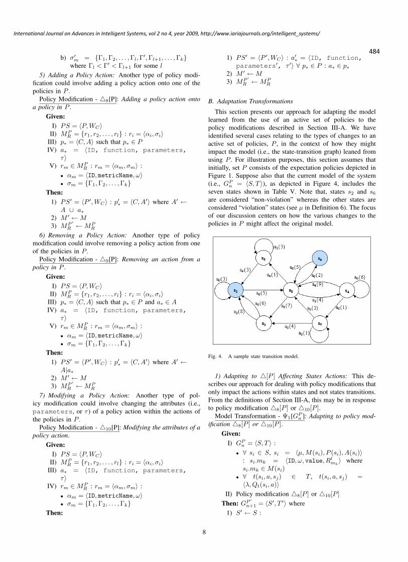
484


b) σ′m = {Γ1,Γ2, . . . ,Γl,Γ′,Γl+1, . . . ,Γk}where Γl < Γ′ < Γl+1 for some l

5) Adding a Policy Action: Another type of policy modi-fication could involve adding a policy action onto one of thepolicies in P .

Policy Modification - 48[P]: Adding a policy action ontoa policy in P .



III) p∗ = 〈C,A〉 such that p∗ ∈ PIV) a∗ = 〈ID, function, parameters,

τ〉V) rm ∈MP

R : rm = 〈αm, σm〉 :• αm = 〈ID, metricName, ω〉• σm = {Γ1,Γ2, . . . ,Γk}

Then:1) PS′ = 〈P ′,WC〉 : p′∗ = 〈C,A′〉 where A′ ←

A ∪ a∗2) M ′ ←M3) MP ′

R ←MPR

6) Removing a Policy Action: Another type of policymodification could involve removing a policy action from oneof the policies in P .

Policy Modification - 49[P]: Removing an action from apolicy in P .



III) p∗ = 〈C,A〉 such that p∗ ∈ P and a∗ ∈ AIV) a∗ = 〈ID, function, parameters,

τ〉V) rm ∈MP


Then:1) PS′ = 〈P ′,WC〉 : p′∗ = 〈C,A′〉 where A′ ←

A|a∗2) M ′ ←M3) MP ′

R ←MPR

7) Modifying a Policy Action: Another type of pol-icy modification could involve changing the attributes (i.e.,parameters, or τ ) of a policy action within the actions ofthe policies in P .

Policy Modification - 410[P]: Modifying the attributes of apolicy action.



III) a∗ = 〈ID, function, parameters,τ〉

IV) rm ∈MPR : rm = 〈αm, σm〉 :

• αm = 〈ID, metricName, ω〉• σm = {Γ1,Γ2, . . . ,Γk}

Then:

1) PS′ = 〈P ′,WC〉 : a′∗ = 〈ID, function,parameters′, τ ′〉 ∀ p∗ ∈ P : a∗ ∈ p∗

2) M ′ ←M3) MP ′

R ←MPR

B. Adaptation Transformations

This section presents our approach for adapting the modellearned from the use of an active set of policies to thepolicy modifications described in Section III-A. We haveidentified several cases relating to the types of changes to anactive set of policies, P , in the context of how they mightimpact the model (i.e., the state-transition graph) leaned fromusing P . For illustration purposes, this section assumes thatinitially, set P consists of the expectation policies depicted inFigure 1. Suppose also that the current model of the system(i.e., GP

n = 〈S, T 〉), as depicted in Figure 4, includes theseven states shown in Table V. Note that, states s2 and s6

are considered “non-violation” whereas the other states areconsidered “violation” states (see µ in Definition 6). The focusof our discussion centers on how the various changes to thepolicies in P might affect the original model.

Fig. 4. A sample state transition model.

1) Adapting to 4[P ] Affecting States Actions: This de-scribes our approach for dealing with policy modifications thatonly impact the actions within states and not states transitions.From the definitions of Section III-A, this may be in responseto policy modification 48[P ] or 410[P ].

Model Transformation - Ψ1[GPn ]: Adapting to policy mod-

ification 48[P ] or 410[P ].Given:

I) GPn = 〈S, T 〉 :

• ∀ si ∈ S, si = 〈µ,M(si), P (si), A(si)〉: si.mk = 〈ID, ω, value, Rl

mk〉 where

si.mk ∈M(si)• ∀ t(si, a, sj) ∈ T , t(si, a, sj) =〈λ, Qt(si, a)〉

II) Policy modification 48[P ] or 410[P ]Then: GP ′

n+1 = 〈S′, T ′〉 where1) S′ ← S :

8

485


f(Rkmj

) A(si) t(si, al, s∗)

si f(Rkm1

) f(Rkm2

) f(Rkm3

) f(Rkm4

) f(Rkm5

) f(Rkm6

) al State action λ s∗

s1 0 0 0 0 0 0

a0 γ-actiona1 AdjustMaxClients(+25) 4 s4

a2 AdjustMaxClients(-25)a4 AdjustMaxKeepAliveRequests(-30) 1 s5

a6 AdjustMaxBandwidth(-128) 7;2 s3;s6

s2 0 100 0 100 0 100 a0 γ-action 5;3 s1;s2

s3 50 100 0 0 100 100 a0 γ-action 6 s2

a2 AdjustMaxClients(-25) 8 s2

s4 0 100 0 100 0 0

a0 γ-action 6 s4

a1 AdjustMaxClients(+25)a4 AdjustMaxKeepAliveRequests(-30) 9 s1

a6 AdjustMaxBandwidth(-128) 1 s7

s5 0 0 100 100 0 0



a6 AdjustMaxBandwidth(-128)s6 50 100 0 100 100 100 a0 γ-action 5 s1

s7 100 100 100 100 100 100a0 γ-action 2 s1


a3 AdjustMaxKeepAliveRequests(+30) 4 s3

TABLE VSAMPLE STATES BASED ON THE METRICS STRUCTURE OF TABLE II AND THE STATE-TRANSITION MODEL OF FIGURE 4.

a) ∀ si ∈ S : p∗ ∈ P ′(si); A′(si) ←A(si) ∪ a∗ (48[P ])

b) ∀ si ∈ S; a∗ ← a′∗ ⇐⇒ ∃ a ∈ A(si) :a∗ = a (410[P ])

2) T ′ ← T

Suppose, for example, that policy modifica-tion 410[P ] involves modifying policy action“AdjustMaxBandwidth(-128)” (which correspondsto action a6 in Table V) to “AdjustMaxBandwidth(-64)” in the policies of Figure 1. The following describesthe steps involved in transforming the state-transition modelof Figure 5(a), whose states are shown in Table V andcorrespond to the steps of model-transformation Ψ1[GP

n ]:

1) For each state that has been encountered to date(see Table V), the agent must update the actionswithin the states to ensure that the appropriate ac-tion is modified (see Step 1(b)). Since action a6

was initially in actions sets A(s1), A(s4), and A(s5),each occurrence of the action would be modifiedto “AdjustMaxBandwidth(-64)” as illustrated inFigure 5(c).

2) This change, however, would not affect the transitionsassociated with the modified action. Consider, for ex-ample, transitions t(s1, a6{7}, s3) and t(s1, a6{2}, s6),both involving action a6 (see Figure 5(a)). The fact thatthe action is still part of the actions within the statesmeans that the agent may still take such transitions.Hence, no changes would be made to the transitionsunless they are encountered in the future, in which caseaction-value estimates and frequencies will be updatesaccordingly.

2) Adapting to 4[P ] Affecting States Transitions: Thisdescribes our approach for dealing with policy modificationsthat only affect the state transitions as a result of modifications

to the composition of policy actions within states. Fromthe definitions of Section III-A, this may be in response topolicy modification 43[P ], 46[P ], or 49[P ]. Our approachessentially involves ensuring that the state transitions set T (si)is consistent with the state actions set A(si).


ification 43[P ], 46[P ], or 49[P ].Given:

I) GPn = 〈S, T 〉 :


mk〉 where


II) Policy modification 43[P ], 46[P ], or 49[P ]Then: GP ′

n+1 = 〈S′, T ′〉 where1) S′ ← S : ∀ si ∈ S ; a ∈ A′(si) ⇐⇒ a ∈{P ′(si) ∪ a0}

2) ∀ t(si, a∗, sj) ∈ T (si) : a∗ /∈ A′(si); T ′ ←T |t(si, a∗, sj)

3) ∀ ai ∈ A(si : ∃ t(si, a, s∗) : si, s∗ ∈ S′,compute Q(si, a) (see Equation 2).

Q(s, a) =∑

ti(s,a,s′j)∈T (s)

Pr[ti(s, a, s′j)]×Qti(s, a) (2)

Suppose, for example, that policy modifi-cation 49[P ] involves deleting policy action“AdjustMaxBandwidth(-128)” (which correspondsto action a6 in Table V) from policy p2 in Figure 1. Thefollowing describes the steps involved in transformingthe state-transition model of Figure 6(a), whose statesare shown in Table V and correspond to the steps ofmodel-transformation Ψ2[GP

n ]:

9

486


(a) Original model: GPn = 〈S, T 〉 (b) New model: GP ′

n+1 = 〈S′, T ′〉

f(Rkmj

) A(si) t(si, al, s∗)si m1 m2 m3 m4 m5 m6 al State action λ s∗

s1 0 0 0 0 0 0




s2 0 100 0 100 0 100 a0 γ-action 5;3 s1;s2

s3 50 100 0 0 100 100 a0 γ-action 6 s2


s4 0 100 0 100 0 0

a0 γ-action 6 s4



s5 0 0 100 100 0 0




s7 100 100 100 100 100 100a0 γ-action 2 s1



(c) System states of the new model.

Fig. 5. State-transition model after 410[P ]; i.e., modifying action a6 =“AdjustMaxBandwidth(-128)” to “AdjustMaxBandwidth(-64)” in thepolicies of Figure 1.

1) Since policy p2 is the only violated policy in state s4,49[P ] would result in the removal of action a6 fromthe actions set A(s4) as illustrated in Figure 6(c). Whilepolicy p2 is also violated in states s1 and s5, 49[P ]would not affect such states. This is because action a6

is also part of other violated policies in those states,such as policy p1 (i.e., a6 ∈ p1) where p1 ∈ P ′(s1) andp1 ∈ P ′(s5).

2) The removal of action a6 from state s4 in the abovestep would mean that transition t(s4, a6{1}, s7) (seeFigure 6(a)) is no longer valid. As such, the transitionwill be removed as illustrated in Figure 6(b).

3) The final step of the adaptation is for the agent toperform backup updates so that any impact on the modelas a result of removing transitions is propagated to theaction-value estimates of the states actions.

3) Adapting to 4[P ] Affecting Metrics Regions: This de-scribes our approach for dealing with policy modifications thataffects the regions within state metrics. From the definitions of

Section III-A, this may be in response to policy modification42[P ], 45[P ], or 47[P ].


ification 42[P ], 45[P ], or 47[P ].

Given:I) GP

n = 〈S, T 〉 :


mk〉 where


II) Policy modification 44[P ] or 45[P ] or 47[P ]

Then: GP ′

n+1 = 〈S′, T ′〉 where

1) S′ ← S : ∀ si ∈ S;

a) si.m.Rlm ← (Γl,Γl+1) : σ′m.Γl <

si.m.value < σ′m.Γl+1

b) a ∈ A′(si) ⇐⇒ a ∈ {P ′(si) ∪ a0}

10

487



n+1 = 〈S′, T ′〉

f(Rkmj


s1 0 0 0 0 0 0




s2 0 100 0 100 0 100 a0 γ-action 5;3 s1;s2

s3 50 100 0 0 100 100 a0 γ-action 6 s2


s4 0 100 0 100 0 0a0 γ-action 6 s4


s5 0 0 100 100 0 0




s7 100 100 100 100 100 100a0 γ-action 2 s1




Fig. 6. State-transition model after 49[P ]; i.e., removing action a6 =“AdjustMaxBandwidth(-128)” from policy p2 in Figure 1.


f(Rjmi

)

m6m6.value ≤ −1.0 R1

m6 1007 APACHE:responseTimeTREND > -1.0 m6.value > −1.0 R2

m6 0

TABLE VIMETRIC m6 STRUCTURE AFTER 47[P ]; I.E., MODIFYING THE THRESHOLD OF CONDITION c7 =“APACHE:responseTimeTREND > 0.0” TO

“APACHE:responseTimeTREND > -1.0” IN THE POLICIES OF FIGURE 1.

2) ∀ t(si, a∗, sj) ∈ T (si) : a∗ /∈ A′(si); T ′ ←T |t(si, a∗, sj)

3) ∀ si, sj ∈ S′ : si = sj where i 6= j;a) T ′(si)← T ′(si) ∪ T ′(sj)∀ t(si, a, s) ∈ T ′(si) and ∀ t′(sj , a

′, s′) ∈T ′(sj) : a = a′ and s = s′;i) Qt(si, a) ←

t.λ×Qt(si, a) + t′.λ×Qt′(sj , a′)

t.λ + t′.λii) t.λ← t.λ + t′.λ

iii) T ′ ← T |t′(sj , a′, s′)

b) S′ ← S′|sj

4) ∀ ai ∈ A(si : ∃ t(si, a, s∗) : si, s∗ ∈ S′,

compute Q(si, a) (see Equation 2).

Suppose, for example, that policy modification 47[P ]involves modifying the threshold of policy conditionc7 =“APACHE: responseTimeTREND > 0.0” (whichcorresponds to metric m6 in Table II) to “APACHE:responseTimeTREND > -1.0” in the policies of Fig-ure 1. Thus, instead of σm6 = {0.0}, as was the caseprior to 47[P ] (see Table II), the new regions will bedefined by σm6 = {−1.0}, as is illustrated in Table VI.Suppose also that the following measurements correspond tothe average value of metric m6; “s2.m6.value = −0.5”,“s3.m6.value = −2.0”, “s6.m6.value = −1.5”, and

11

488



n+1 = 〈S′, T ′〉

f(Rkmj


s1 0 0 0 0 0 0




s24 0 100 0 100 0 0

a0 γ-action 5;9 s1;s24



s3 50 100 0 0 100 100 a0 γ-action 6 s2


s5 0 0 100 100 0 0




s7 100 100 100 100 100 100a0 γ-action 2 s1




Fig. 7. State-transition model after 47[P ]; i.e., modifying the threshold of condition c7 =“APACHE:responseTimeTREND > 0.0” to“APACHE:responseTimeTREND > -1.0” in the policies of Figure 1.

“s7.m6.value = −2.5”. The following describes the stepsinvolved in transforming the state-transition model of Fig-ure 7(a), whose states are shown in Table V and correspondto the steps of model-transformation Ψ3[GP

n ]:1) Since “m6.value < −1.0” in states s3, s6, and s7,

f(Rlm6

) would not be affected by the policy modifica-tion in those states since the measurements would re-main in region R1

m6. However, since “s2.m6.value =

−0.5”, f(Rkm6

) would recompute the region value bychanging it from 100 (see Table V) to 0 since the mea-surement would now fall in region R2

m6(see Table VI)

instead of the previous region R1m6

(see Table II). Theagent must also update the states actions sets of eachstate to ensure that actions set A′(si) contains onlythe actions of the policies that are violated when thesystem is in state si (see Step 1(b)). Note that 47[P ]would result in the violation of policy p2 when theagent is in state s2. This was not the case prior tothe policy modification since only one of the policyconditions was violated. As such, actions a1, a4, and

a6 would be added onto the actions set A(s2); i.e.,A′(s2) = {a0, a1, a4, a6}.

2) Since the previous stage did not result in the deletion ofstates actions, no transition will be affected.

3) Changing the region from R1m6

to R2m6

in state s2

would mean states s2 and s4 are identical; i.e., theyhave the same region value assignment (i.e., f(Rl

mi))

for each identical metric. Thus, the two states wouldbe merged together onto state s24, as illustrated inFigure 7. This would also involve merging the statestransitions such that transition t(s4, a6{1}, s7) becomestransition t(s24, a6{1}, s7), while t(s4, a4{9}, s1) be-comes transition t(s24, a4{9}, s1) (see Step 3(a)). In thecase of two identical transitions such as t(s4, a0{6}, s4)and t(s2, a0{3}, s2), a new transition t(s24, a0{9}, s24)would be formed as illustrated in Figure 7(b) such thatthe frequency of the new transition is the sum of thefrequencies of the two merged transitions. Once thetransitions have been updated, the duplicate state isremoved (see Step 3(b)).

12

489


4) The final step of the adaptation is for the agent toperform backup updates so that any impact on the modelas a result of merging states and transitions is propagatedto the action-value estimates of the states actions.

4) Adapting to 4[P ] Resulting in a Decrease in StateMetrics: This describes our approach for dealing with policymodifications that reduces the size of the metrics set M , pos-sibly resulting in two or more identical states. As mentionedpreviously, two states are said to be identical if they sharethe same metrics region values as determined by the mappingf(Rj

mi) (see Equation 1) based on each metric’s measurement

(i.e., mi.value). From the definitions of Section III-A, thismay be in response to policy modification 44[P ].


ification 44[P ].Given:

I) GPn = 〈S, T 〉 :


mk〉 where


II) Policy modification 44[P ]Then: GP ′

n+1 = 〈S′, T ′〉 where1) S′ ← S : ∀ si ∈ S;

a) M ′(sj) ← M(sj)|m : m is the deletedmetric

b) a ∈ A′(si) ⇐⇒ a ∈ {P ′(si) ∪ a0}2) ∀ t(si, a∗, sj) ∈ T (si) : a∗ /∈ A′(si); T ′ ←

T |t(si, a∗, sj)3) ∀ si, sj ∈ S′ : si = sj where i 6= j;

a) T ′(si)← T ′(si) ∪ T ′(sj)∀ t(si, a, s) ∈ T ′(si) and ∀ t′(sj , a

′, s′) ∈T ′(sj) : a = a′ and s = s′;i) Qt(si, a) ←

t.λ×Qt(si, a) + t′.λ×Qt′(sj , a′)

t.λ + t′.λii) t.λ← t.λ + t′.λ

iii) T ′ ← T |t′(sj , a′, s′)

b) S′ ← S′|sj

4) ∀ ai ∈ A(si : ∃ t(si, a, s∗) : si, s∗ ∈ S′,compute Q(si, a) (see Equation 2).

Suppose, for example, that policy modifica-tion 44[P ] involves removing policy conditionc5 =“MEMORY:utilizationTREND > 0.0” (whichcorresponds to metric m4 in Table II) from policy p4 inFigure 1. The following describes the steps involved intransforming the state-transition model of Figure 8(a), whosestates are shown in Table V and correspond to the steps ofmodel-transformation Ψ4[GP

n ]:1) For each state that has been encountered to date (see

Table V), the agent must first remove all the informationassociated with metric m4 (see step 1(a)). This wouldresult in a system’s model with seven states, each withfive metrics; i.e., M(si) = {m1,m2,m3,m5,m6}. Theagent must also update the states actions sets of each

state to ensure that actions set A′(si) contains onlythe actions of the policies that are violated when thesystem is in state si (see Step 1(b)). Note that 44[P ]would result in the violation of policy p4 when theagent is in states s2, s4, or s6. This was not the caseprior to the policy modification since only one of thepolicy conditions was violated; i.e., f(Rl

m1) = 0 while

f(Rlm4

) = 100. Thus, removing m4 from state theabove states would mean that p4 is now violated. Assuch, action a2 would be added onto actions sets A(s2),A(s4), and A(s6), making states s2 and s6 violationstates.

2) The state-transition model must also be updated toensure that the actions within states transitions areconsistent with the updated states actions sets. Since theprevious stage did not result in the deletion of statesactions, no transition will be affected.

3) The agent must then determine whether any statesshould be merged together if, in fact, the modificationsabove may have resulted in two or more identicalstates. Note that the deletion of metric m4 wouldmean states s3 and s6 are identical; i.e., they havethe same region value assignment (i.e., f(Rl

mi)) for

each identical metric. Thus, the two states would bemerged together onto state s36, as illustrated in Fig-ure 8. This would also involve merging the statestransitions such that transition t(s6, a0{5}, s1) becomestransition t(s36, a0{5}, s1) (see Step 3(a)). In the caseof two identical transitions such as t(s1, a6{2}, s6)and t(s1, a6{7}, s3), a new transition t(s1, a6{9}, s36)would be formed, as illustrated in Figure 8(b), suchthat the frequency of the new transition is the sumof the frequencies of the two merged transitions. Oncethe transitions have been updated, the duplicate state isremoved (see Step 3(b)).

4) The final step of the adaptation is for the agent toperform backup updates so that any impact on the modelas a result of removing transitions and/or merging statesis propagated to the action-value estimates of the statesactions.

5) Adapting to 4[P ] Resulting in an Increase in StateMetrics: This describes our approach for dealing with policymodifications that increase the size of the metrics set M . Fromthe definitions of Section III-A, this may be in response topolicy modification 41[P ].


ification 41[P ].Given:

I) GPn = 〈S, T 〉 :


mk〉 where


II) Policy modification 41[P ]Then: GP ′

n+1 = 〈S′, T ′〉 where1) S′ ← {∅}

13

490



n+1 = 〈S′, T ′〉

f(Rkmj

) A(si) t(si, al, s∗)si m1 m2 m3 m5 m6 al State action λ s∗

s1 0 0 0 0 0




s2 0 100 0 0 100 a0 γ-action 5;3 s1;s2

a2 AdjustMaxClients(-25)

s36 50 100 0 100 100 a0 γ-action 5;6 s1;s2


s4 0 100 0 0 0

a0 γ-action 6 s4

a1 AdjustMaxClients(+25)a2 AdjustMaxClients(-25)a4 AdjustMaxKeepAliveRequests(-30) 9 s1


s5 0 0 100 0 0



a6 AdjustMaxBandwidth(-128)

s7 100 100 100 100 100a0 γ-action 2 s1




Fig. 8. State-transition model after 44[P ]; i.e., deleting condition c5 =“MEMORY:utilizationTREND > 0.0” from policy p4 in Figure 1.


f(Rjmi

)

m710 APACHE:refusedRequests < 10.0 m7.value ≤ 10.0 R1

m7 100m7.value > 10.0 R2

m7 0

TABLE VIIMETRICS m7 STRUCTURE AFTER 41[P ]; I.E., ADDING CONDITION c10 =“APACHE:refusedRequests < 10.0” ONTO POLICY p5 IN FIGURE 1.

2) T ′ ← {∅}Suppose, for example, that policy modifi-

cation 41[P ] involves adding the conditionc10 =“APACHE:refusedRequests < 10.0” ontopolicy p5 in Figure 1. This would result in a new statemetric (i.e., m7 =“APACHE:refusedRequests”) withtwo regions associated with it, whose structure is shown inTable VII. For a system whose model is derived from visitingthe states in Table V, such a change to the policies set Pwould mean a binary split of each of the seven states toaccount for the two regions of the new metric. However, sinceno measurements associated with metrics m7 would have

been collected as was pointed out in Section III-B5, therewould be no way of knowing how to map the old transitionsonto the new states set. As such, 41[P ] is the only policymodification requiring learning a new model from scratch.

C. A Sequence of Transformations

Consider a more complex example where 4[P ] involvesremoving policy p4 in Figure 1; i.e.,


II) p4 = 〈C,A〉 such that p4 ∈ P :

14

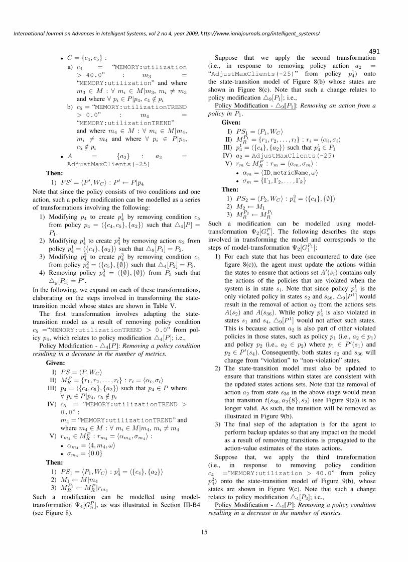
491


• C = {c4, c5} :a) c4 = “MEMORY:utilization

> 40.0” : m3 =“MEMORY:utilization” and wherem3 ∈ M : ∀ mi ∈ M |m3, mi 6= m3

and where ∀ pi ∈ P |p4, c4 /∈ pi

b) c5 = “MEMORY:utilizationTREND> 0.0” : m4 =“MEMORY:utilizationTREND”and where m4 ∈ M : ∀ mi ∈ M |m4,mi 6= m4 and where ∀ pi ∈ P |p4,c5 /∈ pi

• A = {a2} : a2 =AdjustMaxClients(-25)

Then:1) PS′ = 〈P ′,WC〉 : P ′ ← P |p4

Note that since the policy consists of two conditions and oneaction, such a policy modification can be modelled as a seriesof transformations involving the following:

1) Modifying p4 to create p14 by removing condition c5

from policy p4 = 〈{c4, c5}, {a2}〉 such that 44[P ] =P1.

2) Modifying p14 to create p2

4 by removing action a2 frompolicy p1

4 = 〈{c4}, {a2}〉 such that 49[P1] = P2.3) Modifying p2

4 to create p34 by removing condition c4

from policy p24 = 〈{c5}, {∅}〉 such that 44[P2] = P3.

4) Removing policy p34 = 〈{∅}, {∅}〉 from P3 such that

4y[P3] = P ′.In the following, we expand on each of these transformations,elaborating on the steps involved in transforming the state-transition model whose states are shown in Table V.

The first transformation involves adapting the state-transition model as a result of removing policy conditionc5 =“MEMORY:utilizationTREND > 0.0” from pol-icy p4, which relates to policy modification 44[P ]; i.e.,

Policy Modification - 44[P ]: Removing a policy conditionresulting in a decrease in the number of metrics.



III) p4 = 〈{c4, c5}, {a2}〉 such that p4 ∈ P where∀ pi ∈ P |p4, c5 /∈ pi

IV) c5 = “MEMORY:utilizationTREND >0.0” :m4 = “MEMORY:utilizationTREND” andwhere m4 ∈M : ∀ mi ∈M |m4, mi 6= m4

V) rm4 ∈MPR : rm4 = 〈αm4 , σm4〉 :

• αm4 = 〈4,m4, ω〉• σm4 = {0.0}

Then:1) PS1 = 〈P1,WC〉 : p1

4 = 〈{c4}, {a2}〉2) M1 ←M |m4

3) MP1R ←MP

R |rm4

Such a modification can be modelled using model-transformation Ψ4[GP

n ], as was illustrated in Section III-B4(see Figure 8).

Suppose that we apply the second transformation(i.e., in response to removing policy action a2 =“AdjustMaxClients(-25)” from policy p1

4) ontothe state-transition model of Figure 8(b) whose states areshown in Figure 8(c). Note that such a change relates topolicy modification 49[P1]; i.e.,

Policy Modification - 49[P1]: Removing an action from apolicy in P1.

Given:I) PS1 = 〈P1,WC〉

II) MP1R = {r1, r2, . . . , rl} : ri = 〈αi, σi〉

III) p14 = 〈{c4}, {a2}〉 such that p1

4 ∈ P1

IV) a2 = AdjustMaxClients(-25)V) rm ∈MP


Then:1) PS2 = 〈P2,WC〉 : p2

4 = 〈{c4}, {∅}〉2) M2 ←M1

3) MP2R ←MP1

R


n ]. The following describes the stepsinvolved in transforming the model and corresponds to thesteps of model-transformation Ψ2[GP1

1 ]:1) For each state that has been encountered to date (see

figure 8(c)), the agent must update the actions withinthe states to ensure that actions set A′(si) contains onlythe actions of the policies that are violated when thesystem is in state si. Note that since policy p1

4 is theonly violated policy in states s2 and s36, 49[P 1] wouldresult in the removal of action a2 from the actions setsA(s2) and A(s36). While policy p1

4 is also violated instates s1 and s4, 49[P 1] would not affect such states.This is because action a2 is also part of other violatedpolicies in those states, such as policy p1 (i.e., a2 ∈ p1)and policy p2 (i.e., a2 ∈ p2) where p1 ∈ P ′(s1) andp2 ∈ P ′(s4). Consequently, both states s2 and s36 willchange from “violation” to “non-violation” states.

2) The state-transition model must also be updated toensure that transitions within states are consistent withthe updated states actions sets. Note that the removal ofaction a2 from state s36 in the above stage would meanthat transition t(s36, a2{8}, s2) (see Figure 9(a)) is nolonger valid. As such, the transition will be removed asillustrated in Figure 9(b).

3) The final step of the adaptation is for the agent toperform backup updates so that any impact on the modelas a result of removing transitions is propagated to theaction-value estimates of the states actions.

Suppose that, we apply the third transformation(i.e., in response to removing policy conditionc4 =“MEMORY:utilization > 40.0” from policyp24) onto the state-transition model of Figure 9(b), whose

states are shown in Figure 9(c). Note that such a changerelates to policy modification 44[P2]; i.e.,

Policy Modification - 44[P ]: Removing a policy conditionresulting in a decrease in the number of metrics.

15

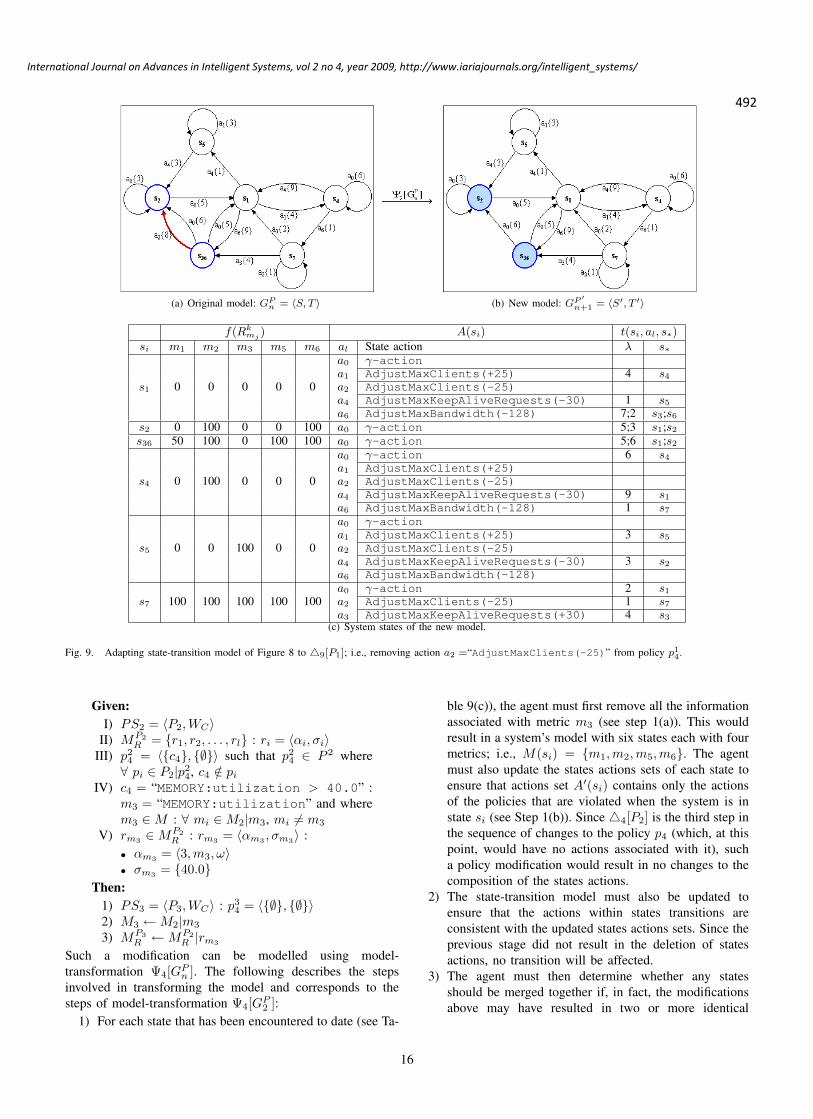
492



n+1 = 〈S′, T ′〉

f(Rkmj

) A(si) t(si, al, s∗)si m1 m2 m3 m5 m6 al State action λ s∗

s1 0 0 0 0 0




s2 0 100 0 0 100 a0 γ-action 5;3 s1;s2

s36 50 100 0 100 100 a0 γ-action 5;6 s1;s2

s4 0 100 0 0 0

a0 γ-action 6 s4

a1 AdjustMaxClients(+25)a2 AdjustMaxClients(-25)a4 AdjustMaxKeepAliveRequests(-30) 9 s1


s5 0 0 100 0 0



a6 AdjustMaxBandwidth(-128)

s7 100 100 100 100 100a0 γ-action 2 s1




Fig. 9. Adapting state-transition model of Figure 8 to 49[P1]; i.e., removing action a2 =“AdjustMaxClients(-25)” from policy p14.



III) p24 = 〈{c4}, {∅}〉 such that p2

4 ∈ P 2 where∀ pi ∈ P2|p2

4, c4 /∈ pi

IV) c4 = “MEMORY:utilization > 40.0” :m3 = “MEMORY:utilization” and wherem3 ∈M : ∀ mi ∈M2|m3, mi 6= m3

V) rm3 ∈MP2R : rm3 = 〈αm3 , σm3〉 :

• αm3 = 〈3,m3, ω〉• σm3 = {40.0}

Then:1) PS3 = 〈P3,WC〉 : p3

4 = 〈{∅}, {∅}〉2) M3 ←M2|m3

3) MP3R ←MP2

R |rm3


n ]. The following describes the stepsinvolved in transforming the model and corresponds to thesteps of model-transformation Ψ4[GP

2 ]:1) For each state that has been encountered to date (see Ta-

ble 9(c)), the agent must first remove all the informationassociated with metric m3 (see step 1(a)). This wouldresult in a system’s model with six states each with fourmetrics; i.e., M(si) = {m1,m2,m5,m6}. The agentmust also update the states actions sets of each state toensure that actions set A′(si) contains only the actionsof the policies that are violated when the system is instate si (see Step 1(b)). Since 44[P2] is the third step inthe sequence of changes to the policy p4 (which, at thispoint, would have no actions associated with it), sucha policy modification would result in no changes to thecomposition of the states actions.

2) The state-transition model must also be updated toensure that the actions within states transitions areconsistent with the updated states actions sets. Since theprevious stage did not result in the deletion of statesactions, no transition will be affected.

3) The agent must then determine whether any statesshould be merged together if, in fact, the modificationsabove may have resulted in two or more identical

16

493



n+1 = 〈S′, T ′〉

f(Rkmj

) A(si) t(si, al, s∗)si m1 m2 m5 m6 al State action λ s∗

s15 0 0 0 0

a0 γ-actiona1 AdjustMaxClients(+25) 3;4 s15;s4

a2 AdjustMaxClients(-25)a4 AdjustMaxKeepAliveRequests(-30) 1;3 s15; s2


s2 0 100 0 100 a0 γ-action 5;3 s15;s2

s36 0 100 100 100 a0 γ-action 5;6 s15;s2

s4 0 100 0 0

a0 γ-action 6 s4



s7 100 100 100 100a0 γ-action 2 s15




Fig. 10. Adapting state-transition model of Figure 9 to 44[P2]; i.e., removing condition c4 =“MEMORY:utilization > 40.0” from policy p24.

states. Note that the deletion of metric m3 wouldmean states s1 and s5 are identical; i.e., they havethe same region value assignment (i.e., f(Rl

mi)) for

each identical metric. Thus, the two states would bemerged together into state s15 as illustrated in Figure 10.This would also involve merging the states transitions(see Step 3(a)) such that, transitions t(s1, a4{1}, s5),t(s5, a1{3}, s5), and t(s5, a4{3}, s2) (see Figure 10(a))become transitions t(s15, a4{1}, s15), t(s15, a1{3}, s15),and t(s15, a4{3}, s2), respectively (see Figure 10(b)).

4) The final step of the adaptation is for the agent toperform backup updates so that any impact on the modelas a result of removing transitions and/or merging statesis propagated to the action-value estimates of the statesactions.

Finally, we apply the fourth transformation (i.e., in responseto removing policy p3

4) onto the state-transition model ofFigure 10(b), whose states are shown in Figure 10(c). Notethat such a change relates to policy modification 4y[P3]; i.e.,

Policy Modification - 4y[P3]: Removing a policy withoutconditions or actions.



III) p34 = 〈∅, ∅〉 such that p3

4 ∈ P3

Then:1) PS′ = 〈P ′,WC〉 : P ′ ← P3|p3

4

2) M ′ ←M3

3) MP ′

R ←MP3R

Since 4y[P3] has no impact on the state-transition model,removing policy p3

4 from Figure 1 would result in no changesto the state-transition model of Figure 10. As such, the removalof policy p4 can be modelled as a sequence of transformationson the original state-transition model involving: 44[P ] = P1,49[P1] = P2, 44[P2] = P3, and 4y[P3] = P ′.

IV. EXPERIENCE

In this section, we present experiments illustrating theeffectiveness of the adaptation mechanisms on the behaviorof the server in response to run-time policy modifications. Inparticular, we compare results from two experimental settingsbased on how the agent responded to run-time policy modifi-cations. The first experiment (EXP-1) investigated the behaviorof the server where the learning agent discards everything itmay have learned prior to 4[P ] and begins learning fromscratch; i.e., GP ′

n+1 = {∅, ∅}. The second experiment (EXP-2)looked at the behavior of the server where the learning agentadapts the model of the environment dynamics to take intoaccount the changes to an active set of policies, essentially

17

494


(a) Response Time

(b) CPU Utilization

(c) Throughput

Fig. 11. Adapting to run-time policy modification: 4[P ] involves replacing “mixed” expectation policies with “simple” expectation policies

reusing some of the learned information; i.e., Ψ : GPn → GP ′

n+1

(see Figure 3).

A. Testbed EnvironmentOur testbed consisted of a collection of networked work-

stations: an administrative workstation to run the experiments;a Linux workstation with a 2.0 GHz processor and 2.0 Gbof memory, which hosted the Apache Web Server along withthe PHP module and the MySQL database server; and threeworkstations used for generating the server’s workload, whichconsisted of clients requests associated with gold, silver, andbronze service classes.

To emulate the stochastic behavior of users, an Apachebenchmark tool called JMeter [12] was used. The tool pro-vides support for concurrent sampling of requests through amulti-threaded framework. It provides the ability to specifythe client’s think time as well as the number of concurrent- independent - keep-alive connections. In the experimentsreported here, these values were set to ensure that the serverwas under overload conditions (i.e., saturated) for the entireduration of the experiments. In our current implementation,the tool has been configured to traverse a Web graph of anactual Web site: in our case, phpBB [13]. In the experimentsreported in this section, only read-only database requests were

18

495


considered.In order to support service differentiation, a Linux Traffic

Controller (TC) was used to configure the bandwidth associ-ated with the gold, silver, and bronze service classes. The ser-vice classes bandwidth was assigned proportionately accordingto the ratio 85:10:5. Bandwidth sharing was also permitted.The tuning parameter MaxBandwidth is what determineshow much bandwidth is assigned to each service class. Itcorresponds to the physical capacity (in kbps) of the networkconnection to the workstation hosting the servers. Thus, giventhat the first policy of Figure 1 has been violated and thatit is no longer possible, for example, to adjust the parametersMaxClients and MaxKeepAliveRequests, then the lastpolicy action (i.e., AdjustMaxBandwidth(-128)) wouldbe executed. This action essentially reduces the total band-width by 128 kbps. The percentage of the new bandwidth iswhat is eventually assigned to the different service classes.

B. Results

The results presented in this section aim at demonstratingthe effectiveness of the adaptation mechanisms on the policymodifications involving changing policy sets. Two sets ofpolicies were considered and included “simple” and “mixed”expectation policies. Simple expectation policies includedpolicies describing possible sets of actions to be taken when-ever a single objective is violated. Mixed expectation policiesinclude policies consisting of both “simple” and “complex”policies, with complex expectation policies describing theactions of the system whenever several objectives are violated.4[P ], in this case, involved replacing “mixed” expectationpolicies with “simple” expectation policies; i.e., disabling allthe complex policies within the mixed expectation policiesset. The performance comparisons in terms of the averagesand magnitude of violations reported in this section focusedspecifically on the behavior of the server after 4[P ] occurred.

Figure 11 shows the behavior of the server when dealingwith the above policy modification, which occurred at about1,900 seconds after the start of the experiment. In terms ofresponse time measurements (see Figure 11(a)), the qualityof service specific to the violations as well as the stabilityof the measurements greatly improved after 4[P ] occurred.This is clearly visible in the graph where there are very fewinstances where the measurements exceeded the threshold.The same is also true when CPU utilization and throughputmeasurements are considered, as Figures 11(b) and 11(c),respectively, illustrate. Thus, the overall quality of servicegreatly improved as a result of the adaptation mechanisms.

The top graph of Figure 12 compares the average through-put measurements of identical service classes. EXP-1 cor-responded to the case where the learning agent discardedeverything it had learned prior to 4[P ] and began learningfrom scratch, while EXP-2 corresponded to the experimentwhere the agent adapted the model in response to the policymodification. Thus, results reported for EXP-2 are essentiallythose of Figure 11, but whose averages only include themeasurements after 4[P ] occurred. From these results, theserver performed slightly better in EXP-2 when compared

to the results in EXP-1, particularly for the gold serviceclass where more requests were served. For the other classes(i.e., silver and bronze), however, the performance gains werestatistically insignificant since the measurements fell withinthe standard error, as is illustrated by the error bars associatedwith the mean throughput.

Fig. 12. Mean performance comparisons.

The same was also true when clients response time mea-surements across the service classes were compared as shownin the bottom graph of Figure 12. Thus, we can concludethat, model adaptation had a positive impact on the overallperformance of the server when averages associated with theserver’s throughput and clients response times were consid-ered. That is, the server performed slightly better in EXP-2 when compared to the results in EXP-1, particularly forthe gold service class where more requests were served.For the other classes (i.e., silver and bronze), however, theperformance differences were statistically insignificant sincethe measurements fell within the standard error.

While the results above show slight improvement in theoverall quality as a result of the adaptation mechanisms, meanperformance is essentially an approximation of the quality ofservice performance of the system. The more accurate measureis the severity and the frequency with which performanceobjectives are violated, as summarized in Figure 13. Note that,EXP-2 recorded at least an 80% reduction in the magnitudeof response time violations (see Figure 13(a)) and a 96%reduction in the magnitude of CPU utilization violations (seeFigure 13(b)). Thus, reducing the magnitude of violationssuch as instances in which clients requests wait on a server’squeue for longer than 2500 ms, for example, is likely to

19

496


(a) Response Time (b) CPU Utilization

Fig. 13. Magnitude of violations performance comparisons.

improve the quality of service from a user’s prospective -a measure mean performance tend to obscure. Furthermore,performance objective under these kinds of environmentsoften need to account for not only customers’ needs, butalso system’s constraints. For example, in order to controlpower consumption, an autonomic system may need to limitCPU utilization. Thus, the ability to achieve system-wideperformance objectives, which may seem conflicting at times,under dynamically changing configuration conditions is whatthe experiments presented in this paper have demonstrated.

Furthermore, the results summarized in this section high-light one of the key benefits of utilizing reinforcement learningmethodologies in policy-driven autonomic management, par-ticularly when it comes to policy specification. That is, very“simple” expectation policies are sufficient to deliver signifi-cant performance gains. With learning enabled, more complexpolicies, particularly those spanning multiple objectives, couldbe learned instead of requiring systems administrators tomanually encode into a single policy how systems shouldachieve multiple objectives. Thus, a general knowledge ofthe performance impact due to a change in the value of aparameter is sufficient to define simple but effective policies.This can significantly reduce the burden faced by humanadministrators, by having them specify simple policies, leavingit to autonomic systems to figure out how to achieve morecomplex objectives.

V. RELATED WORK

Policy-based management approaches have attracted signif-icant interest within autonomic computing. The work in [14],for example, proposes a flexible policy-expression languagecalled AGILE [15], which facilitates run-time policy con-figuration and adaptation of autonomic systems. AGILE initself is both a policy expression language and a frameworkthat facilitates dynamic composition of autonomic techniquesincluding signal processing, trend analysis, and utility func-tions. IBM [6] has also been at the forefront in policy-drivenautonomic management research. Their work in [16] proposesan Agent Building and Learning Environment (ABLE) capableof configuring new behaviors and capabilities to intelligentautonomic systems. In this approach, policies are specified

using rule beans which make use of simple scripting text orExtensible Markup Language (XML) [17] to define simple as-signments including if-then, if-then-else rules, when-do patternmatch rules, etc.

Policy-based management has recently evolved to recognizethe need to evaluate the correctness and effectiveness of poli-cies specified by system administrators. For example, there hasbeen some interest in policy conflicts detection and resolution(see, for example, [18]). Others have proposed frameworks thatmake use of event calculus (EC) [19] for policy verificationswhich adds the notion of time for first-order predicate logic. Itprovides a formalism for representation and reasoning aboutactions and their effects. This approach, however, requires thatrules are specified to identify all possible inconsistencies froma set of policies, which is intractable for complex systems. Thisis particularly the case because, in most situations, some of thecharacteristics for identifying conflicts can only be detected atrun-time.

The need to dynamically adapt the use of policies inautonomic management has also gained some traction. Thework in [20], for example, proposes an adaptive policy-based framework that support dynamic policy configurationin response to changes within the managed environment.In their approach, policy adaptation describes the ability tomodify network behavior by dynamically changing the policyparameters as well as selecting, enabling, or disabling policiesat run-time. Reconfiguration events are used to trigger high-level control policies, which then determines which lower-level policies must be adapted to reconfigure the managedsystem. They use the Ponder deployment framework [21] todistribute policies to the different management components.They describe several ways in which the system’s behaviorcould be adapted by changing the way policies are used [20]:

• Dynamic Modification of Policy Parameters: In this ap-proach, the system can adapt policies by making changesto the policy parameters. This may involve computingnew attribute values based, for example, on Service LevelAgreements (SLAs), resource availability, etc. Relatedwork on this type of adaptation in the use of policiescan be found in [20], [22].

• Enabling/Disabling Policies From a Set of Active Poli-cies: In this approach, the system can use run-timecontext to dynamically use the information provided bythe policies, such as enabling/disabling a policy undercertain circumstances or selecting actions based on con-text. Related work on adaptation through policy selectioncan be found in [20], [23].

• Adaptation By Learning: In this approach, the system candetermine policy use through some learning mechanismsbased on past experience in the use of policies. This typeof adaptation is still in its very early stages, particularlyin the filed of autonomic management, with the majorityof the research work focusing on learning high-levelpolicies. The most recent work can be found in [24],[25], [26], [27].

Our interest is on how learning approaches could facili-tate dynamic use of policies within autonomic computing.

20

497


In our most recent work [7], we have explored the use ofReinforcement Learning methodologies in providing guidanceto the autonomic system in terms of how to effectively useexisting policies. One drawback to this and other approacheswas that when policies change, the existing model is discardedand the system must learn a new model of the environmentfrom scratch. Our experience, however, suggest that policymodifications are frequently “incremental” - e.g., a change toa threshold, the disabling of a single policy, etc. The abilityto reuse a learned model, or part there of, has the potentialbenefit of significantly accelerating the learning process, asthis paper has demonstrated.

VI. CONCLUSION

The approach taken in this paper is only the first step in thebroader goal of developing adaptive policy driven autonomicsolutions involving multiple agents working together towards aset of common, and at times seemingly competing, objectives.This is often the case since performance objectives may needto account for both customers needs and systems constraints.The complexity of today’s IT infrastructure, however, meansthat we can no longer depend on centralized approaches to per-formance management. It is becoming increasingly commonto find multiple agents coexisting within a single computingenvironment. The work in [28], for example, proposes an ap-proach for coordinating two independent autonomic managers:one designed to address power consumption objectives whileanother deals with performance objectives such as responsetime based on some learning mechanisms. As such, policymodifications directives could come not only from the usersof the systems, but also from other autonomic managers. Thefact that our approach to modelling the learning process isdependent only on the structure of the policies means thatsuch changes to policies could be traced back to the modelderived from the use of those policies. In this paper, we haveelaborated on how a model learned from the use of an activeset of policies could be adapted (i.e., reused) to cope withrun-time policy modifications.

While the initial results are encouraging, we intend tovalidate these approaches with a comprehensive prototypeevaluating the impact of the different kinds of policy modifi-cations on the effectiveness of the adaptation transformations.We are also working on formulating formal proofs that showthat, indeed if P is changed to P ′ and GP

n is transformed toGP ′

n+1, then GP ′

n+1 is a model of P ′.

REFERENCES

[1] N. Damianou, N. Dulay, E. C. Lupu, and M. S. Sloman, “Ponder:A Language for Specifying Security and Management Policies forDistributed Systems: The Language Specification,” Imperial College,London, England, Version 2.2, 2000.

[2] (2009, December) The Internet Engineering Task Force (IETF).[Online]. Available: http://www.ietf.org/

[3] (2009, December) The Distributed Management Task Force (DMTF).[Online]. Available: http://www.dmtf.org/

[4] (2009, December) The Object Management Group (OMG). [Online].Available: http://www.omg.org/

[5] (2009, December) Policy Research Group. Imperial College. [Online].Available: http://www-dse.doc.ic.ac.uk/Research/policies/ponder.shtml

[6] (2009, December) Autonomic Computing Research. IBM. [Online].Available: http://www.research.ibm.com/autonomic/

[7] R. M. Bahati and M. A. Bauer, “Modelling Reinforcement Learning inPolicy-driven Autonomic Management,” in IARIA International JournalOn Advances in Intelligent Systems, vol. 1, no. 1, December 2008.

[8] R. M. Bahati and M. A. Bauer, “Adapting to Run-time Changes inPolicies Driving Autonomic Management,” in International Conferenceon Autonomic and Autonomous Systems (ICAS’08), Guadeloupe, March2008, pp. 88–93.

[9] R. M. Bahati, M. A. Bauer, C. Ahn, O. K. Baek, and E. M. Vieira,“Using Policies to Drive Autonomic Management,” in WoWMoM-2006Workshop on Autonomic Communications and Computing (ACC’06),Buffalo, NY, USA, June 2006, pp. 475–479.

[10] R. S. Sutton and A. G. Barto, Reinforcement Learning: an Introduction.Cambridge, MA, USA: MIT Press, 1998.

[11] C. Watkins, “Learning from Delayed Rewards,” Ph.D. dissertation,Cambridge University, Cambridge, UK, 1989.

[12] (2009, December) Apache JMeter. The Apache Software Foundation.[Online]. Available: http://jakarta.apache.org/jmeter/

[13] (2009, December) PHP Bulletin Board. [Online]. Available:http://www.phpbb.com/

[14] R. J. Anthony, “Policy-centric Integration and Dynamic Compositionof Autonomic Computing Techniques,” in International Conference onAutonomic Computing (ICAC’07), Jacksonville, FL, USA, June 2007.

[15] (2009, December) AGILE. [Online]. Available:http://www.policyautonomics.net/

[16] J. P. Bigus, D. A. Schlosnagle, J. R. Pilgrim, W. N. M. III, and Y. Diao,“ABLE: A toolkit for Building Multiagent Autonomic Systems,” in IBMSystems Journal, vol. 41, no. 3, September 2002.

[17] (2009, December) Extensible Markup Language (XML). [Online].Available: http://www.w3.org/XML/

[18] N. Dunlop, J. Indulska, and K. Raymond, “Dynamic Conflict Detectionin Policy-Based Management Systems,” in International EnterpriseDistributed Object Computing Conference (EDOC’02), Washington,DC, USA, 2002, pp. 15–26.

[19] R. Kowalski and M. Sergot, “A Logic-based Calculus of Events,” in NewGeneration Computing, vol. 4, no. 1, Tokyo, Japan, 1986, pp. 67–95.

[20] L. Lymberopoulos, E. C. Lupu, and M. S. Sloman, “An Adaptive Policy-Based Framework for Network Services Management,” in Journal ofNetworks and Systems Management, vol. 11, no. 3, 2003, pp. 277–303.

[21] N. Dulay, E. C. Lupu, M. S. Sloman, and N. Damianou, “A Policy De-ployment Model for the Ponder Language,” in IEEE/IFIP InternationalSymposium on Integrated Network, Seattle, CA, USA, May 2001, pp.529–544.

[22] K. Yoshihara, M. Isomura, and H. Horiuchi, “Distributed Policy-basedManagement Enabling Policy Adaptation on Monitoring using ActiveNetwork Technology,” in IFIP/IEEE International Workshop on Dis-tributed Systems: Operations and Management (DSOM’01), Nancy,France, October 2001.

[23] R. M. Bahati, M. A. Bauer, and E. M. Vieira, “Adaptation Strategiesin Policy-Driven Autonomic Management,” in International Conferenceon Autonomic and Autonomous Systems (ICAS’07), July 2007.

[24] G. Tesauro, N. K. Jong, R. Das, and M. N. Bennani, “A Hybrid Re-inforcement Learning Approach to Autonomic Resource Allocation,” inInternational Conference on Autonomic Computing (ICAC’06), Dublin,Ireland, June 2006, pp. 65–73.

[25] G. Tesauro, “Online Resource Allocation Using Decompositional Rein-forcement Learning,” in National Conference on Artificial Intelligence(AAAI’05), Pittsburgh, PA, USA, 2005, pp. 886–891.

[26] D. Vengerov and N. Iakovlev, “A Reinforcement Learning Frameworkfor Dynamic Resource Allocation: First Results,” in International Con-ference on Autonomic Computing (ICAC’05), Seattle, WA, USA, January2005, pp. 339–340.

[27] P. Vienne and J.-L. Sourrouille, “A Middleware for Autonomic QoSManagement based on Learning,” in International Conference onSofware Engineering and Middleware, Lisbon, Portugal, September2005, pp. 1–8.

[28] J. O. Kephart, H. Chan, R. Das, D. W. Levine, G. Tesauro, F. Raw-son, and C. Lefurgy, “Coordinating Multiple Autonomic Managers toAchieve Specified Power-performance Tradeoffs,” in International Con-ference on Autonomic Computing (ICAC’07), Jacksonville, FL, USA,June 2007.

21

www.iariajournals.org

International Journal On Advances in Intelligent Systems

ICAS, ACHI, ICCGI, UBICOMM, ADVCOMP, CENTRIC, GEOProcessing, SEMAPRO,BIOSYSCOM, BIOINFO, BIOTECHNO, FUTURE COMPUTING, SERVICE COMPUTATION,COGNITIVE, ADAPTIVE, CONTENT, PATTERNS

issn: 1942-2679

International Journal On Advances in Internet Technology

ICDS, ICIW, CTRQ, UBICOMM, ICSNC, AFIN, INTERNET, AP2PS, EMERGING

issn: 1942-2652

International Journal On Advances in Life Sciences

eTELEMED, eKNOW, eL&mL, BIODIV, BIOENVIRONMENT, BIOGREEN, BIOSYSCOM,BIOINFO, BIOTECHNO

issn: 1942-2660

International Journal On Advances in Networks and Services

ICN, ICNS, ICIW, ICWMC, SENSORCOMM, MESH, CENTRIC, MMEDIA, SERVICECOMPUTATION

issn: 1942-2644

International Journal On Advances in Security

ICQNM, SECURWARE, MESH, DEPEND, INTERNET, CYBERLAWS

issn: 1942-2636

International Journal On Advances in Software

ICSEA, ICCGI, ADVCOMP, GEOProcessing, DBKDA, INTENSIVE, VALID, SIMUL, FUTURECOMPUTING, SERVICE COMPUTATION, COGNITIVE, ADAPTIVE, CONTENT, PATTERNS

issn: 1942-2628

International Journal On Advances in Systems and Measurements

ICQNM, ICONS, ICIMP, SENSORCOMM, CENICS, VALID, SIMUL

issn: 1942-261x

International Journal On Advances in Telecommunications

AICT, ICDT, ICWMC, ICSNC, CTRQ, SPACOMM, MMEDIA

issn: 1942-2601

international journal on advances in intelligent systems

Documents