international journal of information technology applications€¦ · paper submission deadline –...
TRANSCRIPT


International Journal of Information Technology Applications
International Journal of
Information Technology Applications (ITA)
Volume 8, Number 1, July 2019
AIMS AND SCOPE OF ITA
The primary aim of the International Journal of Information Technology Applications (ITA) is to
publish high-quality papers of new development and trends, novel techniques, approaches and
innovative methodologies of information technology applications in the broad areas. The
International Journal of ITA is published twice a year. Each paper is refereed by two international
reviewers. Accepted papers will be available online with no publication fee for authors. The journal
is listed in the database of the Russian Science Citation Index (RSCI). The International Journal of
ITA is being prepared for the bibliographic scientific database Scopus.
Editor-in-Chief
prof. RNDr. Frank Schindler, PhD. Faculty of Informatics, Pan-European University in Bratislava
Executive Editor
Ing. Juraj Štefanovič, PhD., Faculty of Informatics, Pan-European University in Bratislava
Editorial Board
Ladislav Andrášik, Slovakia
Mikhail A. Basarab, Russia
Ivan Brezina, Slovakia
Yakhua G. Buchaev, Russia
Oleg Choporov, Russia
Silvester Czanner, United Kingdom
Andrej Ferko, Slovakia
Vladimír S. Galayev, Russia
Ladislav Hudec, Slovakia
Jozef Kelemen, Czech Republic
Sergey Kirsanov, Russia
Vladimir I. Kolesnikov, Russia
Štefan Kozák, Slovakia
Vladimír Krajčík, Czech Republic
Ján Lacko, Slovakia
Igor Lvovich, Russia
Eva Mihaliková, Slovakia
Branislav Mišota, Slovakia
Martin Potančok, Czech Republic
Eugen Ružický, Slovakia
Václav Řepa, Czech Republic
Jiří Voříšek, Czech Republic

International Journal of Information Technology Applications
International Journal of
Information Technology Applications (ITA)
Published with support from
Instructions for authors
The International Journal of Information Technology Applications is welcoming contributions
related with the journal´s scope. Scientific articles in the range approximately 10 standard pages
are reviewed by two international reviewers. Reports up to 5 standard pages and information
notices in range approximately 1 standard page are accepted after the decision of editorial board.
Contributions should be submitted via e-mail to the editorial office. The language of
contributions is English. Text design should preserve the layout of the template file, which may
be downloaded from the webpage of journal. Contributions submitted to this journal are under
the author´s copyright responsibility and they are supposed not being published in the past.
Deadlines of two standard issues per year
paper submission deadline – end of May/end of October
review deadline – continuous process
camera ready deadline – end of June/end of November
release date – July/December
Editorial office address
Faculty of Informatics, Pan-European University, Tematínska 10, 851 05 Bratislava, Slovakia
Published by
Pan-European University, Slovakia, http://www.paneurouni.com
Civil Association EDUCATION-SCIENCE-RESEARCH, Slovakia, http://www.e-s-r.org
Electronic online version of journal
http://www.paneurouni.com/ITA visit Archive, visit Instructions for authors:
http://www.e-s-r.org
Multigrafika s.r.o., Rajecká 13, 821 07 Bratislava
Subscription
Contact the editorial office for details.
Older print issues are available until they are in stock.
ISSN: 2453-7497 (online)
ISSN: 1338-6468 (print version) Registration No.: EV 4528/12

Information Technology Applications
1
Contents
Editorial
Research papers
CONTRIBUTION TO THERMAL ANALYSIS
OF THE AIR-COOLED PEM FUEL CELL
Viktor Ferencey, Michal Stromko, Kristián Ondrejička . . . . . . . . . . . . . . . . . . . . . . . . . . . . . .
3
POWER SYSTEM FLEXIBILITY METRICS REVIEW
WITH HIGH PENETRATION OF VARIABLE RENEWABLE GENERATION
M. Saber Eltohamy, M. Said Abdel Moteleb, Hossam Talaat,
S. Fouad Mekhemer, Walid Omran . . . . . . . . . . . . . . . . . . . . . . . . . . . . . . . . . . . . . . . . . . . . .
21
FEATURES OF THE IMPLEMENTATION OF TIME MANAGEMENT
TECHNIQUES IN THE PROGRAMMING LANGUAGE DART
Yakov Lvovich, Emma Lvovich . . . . . . . . . . . . . . . . . . . . . . . . . . . . . . . . . . . . . . . . . . . . . . . .
47
AUTOMATED WORKPLACE FOR THE DEVELOPMENT
OF ELECTRONIC COMPONENTS
Andrey Preobrazhenskiy, Yakov Lvovich, Juraj Štefanovič . . . . . . . . . . . . . . . . . . . . . . . . . .
57
COMPUTATIONAL MECHANICS AND OPTIMAL PROGRAMMING PARADIGM
Michal Kráčalík . . . . . . . . . . . . . . . . . . . . . . . . . . . . . . . . . . . . . . . . . . . . . . . . . . . . . . . . . . . . . . . .
69
INVESTIGATION OF IMAGE RECONSTRUCTION ALGORITHM
BASED ON THE STRUCTURED LIGHT METHOD
Igor Lvovich, Oleg Choporov, Eugen Ružický . . . . . . . . . . . . . . . . . . . . . . . . . . . . . . . . . . . .
75
DEVELOPMENT OF AN APPLICATION FOR THE E-STORE ON ANDROID
Andrey Preobrazhenskiy, Emma Lvovich, Kseniya Lvovich . . . . . . . . . . . . . . . . . . . . . . . . .
87
IMPLEMENTATION AND TESTING OF TEXT RECOGNITION ALGORITHM
ON MOBILE DEVICES
Oleg Choporov, Igor Lvovich, Juraj Štefanovič . . . . . . . . . . . . . . . . . . . . . . . . . . . . . . . . . . . . .
99
List of Reviewers . . . . . . . . . . . . . . . . . . . . . . . . . . . . . . . . . . . . . . . . . . . . . . . . . . . . . . . . . . . . . . . . . . . .
117

Information Technology Applications
2
Editorial . . . . . . . . . . . . . . . . . . . . . . . . . . . . . . . . . . . . . . . . . . . . . . . . . . . . . . . . . . . . . . . . . . . . . . . . .
Dear authors, dear readers,
contributions in this issue are oriented to applied information technologies in wide spectrum,
including energy production and distribution, data management, programming and image processing.
The fact that information technology is penetrating into all areas of our life is also evidenced by the
content of this journal issue. We offer you an application of algorithms and methods in a wide
spectrum of application area. IT methods and algorithms for modern cars are an integral part of
optimizing their movement. Likewise, modern power engineering uses new forms of energy
production from various sources and by implementing algorithms and methods we can develop an
optimal control for these complex systems. In the present issue of the journal we offer the application
of informatics and effective methods for solving mathematical modeling problems in applied
mechanics. In the area of text recognition, two issues are presented with practical use and verification
of this methodology.
I would like to thank to all concerned people for collaborating, sending articles and correcting them.
New papers and contributions are welcomed around the year.
I wish you a pleasant reading of the published contributions.
Juraj Štefanovič
ITA Editor-in-Chief
Dear authors, dear readers,
This issue brings a ...
New papers and contributions are welcomed around the year. I would like to
thank to all concerned people for collaborating, sending articles and correcting them.
Juraj Štefanovič
ITA Editor-in-Chief

3
International Journal
Information Technology Applications (ITA)
Volume 8, Number 1, July 2019
CONTRIBUTION TO THERMAL ANALYSIS
OF THE AIR-COOLED PEM FUEL CELL
Viktor Ferencey, Michal Stromko, Kristián Ondrejička
Abstract:
This contribution deals with thermal modelling and experimental analysis of the air-cooled PEM (Pro-
ton Exchange Membrane) fuel cell for power systems of transportation applications. The technology of
the energy conversion which directly converts chemical energy of the fuel (hydrogen fuel) into electrical
energy presents a potential replacement for the conventional internal combustion engine (ICE) in trans-
portation applications. PEM fuel cell is an electrochemical energy conversion device which converts
chemical energy of hydrogen and oxygen directly and efficiently into electrical energy with waste heat
and liquid water as by-products of the reaction. There is a number of advantages to a PEM fuel cell
powered electromobiles that use hydrogen such as energy efficient and environmentally benign low
temperature operation, quick start-up, compatibility with renewable energy sources and ability to ob-
tain a power density competitive with the internal combustion engine in the perspective. This paper
explores the limits of using the air cooling for Polymer Electrolyte Membrane (PEM) stacks. Thermal
analysis of the air-cooled fuel cells is, however, a major problem that stems from a low operating tem-
peratures of PEM fuel cell stacks in contrast to the conventional internal combustion engines. In the
present study, a numerical thermal model is presented in order to analyse the heat transfer and predict
the temperature distribution in air-cooled PEM fuel cells. In order to validate the performance of the
created analytical simulation model, comparisons of the data obtained through experimental measure-
ments in the Fuel Cells laboratory have been made.
Keywords:
PEM fuel cells, power system, thermal engineering, temperature, heat transfer, air cooling,
hydrogen fuel, electrochemical device, conversion, temperature distribution.
ACM Computing Classification System:
Temperature simulation and estimation, renewable energy, reusable energy storage.
Introduction
The Proton Exchange Membrane Fuel Cell (PEMFC) is very flexible in terms of its power
and capacity requirements, its long-life service, good ecological balance and very low self-discharges
[1].
PEMFC offers high power density, quick start-up and low operating temperatures as well as
rapid response to varying operational loads in many applications [2]. Currently, a PEMFC with a net
power density of 1kW/L has been achieved [3].
Air-cooled proton exchange membrane fuel cells (PEMFCs), combining air cooling and oxi-
dant supply channels, offer a significantly reduced bill of materials and system complexity compared
to the conventional, water-cooled fuel cells. In air-cooled PEMFC systems, ambient air is applied
freely as the cooling medium which means that the cooling environment is highly influenced by the
ambient temperature. High inlet air temperature would reduce the cooling efficiency.
Viktor Ferencey, Michal Stromko, Kristián Ondrejička
4
Air-cooled fuel cell systems combine the cooling function with the cathode flow field and
reduce overall cost by eliminating a lot of auxiliary systems required for conventional fuel cell de-
signs (water cooling loop, air compressor and humidifier) [4].
Operation of a proton exchange membrane fuel cell (PEMFC) is a complex process that in-
cludes electrochemical reactions coupled with transport of mass, momentum, energy and electricity
[5].
The operating conditions for the best performance require a balance between temperature,
humidity and reactant flow rates in order to avoid flooding of electrodes [6]. The sensitivity of PEM
fuel cell stacks to temperature is mainly related to the required moisture levels in the membrane that
is hydrated from water back-diffusion flux from the cathode to the anode. When the operating current
density increases, the effects of temperature on membrane hydration decrease slightly.
However, heat is also needed for improved reaction kinetics at the catalyst layers. The effects
of the heat to the operation of a fuel cell are subjective and complex. Heat is needed to improve the
reaction kinetics, but too much heat would lead to an increase in energy losses [7]. Therefore, thermal
management of PEM fuel cells needs to balance delicately with both requirements.
The Proton Exchange Membrane Fuel Cell (PEMFC) is very flexible in terms of power and
capacity requirements, its long-life service, good ecological balance and very low self-discharges
[4].
Temperature is a crucial parameter for PEM fuel cell performance which directly or indirectly
affects the reaction kinetics, transport of water, humidity level, conductivity of membrane, catalyst
tolerance, removal of heat or thermal stresses in the membrane etc [4].
To conclude, the performance of the fuel cell increases as the temperature increases from
room temperature to 80°C, further increase in temperature results in a current density dependent
performance. The best performance was observed at around 80°C with 3 bars of absolute back pres-
sure and 100% relative humidity.
For small size and performance of stacks (below 100W), the cooling can be achieved only
with cathode air flow. A disadvantage here is that it requires relatively bigger channel size for cathode
side of the stack compared with the anode side which consequently increases the volume of the stack.
Stacks bigger than few hundred watts require a separate cooling channels.
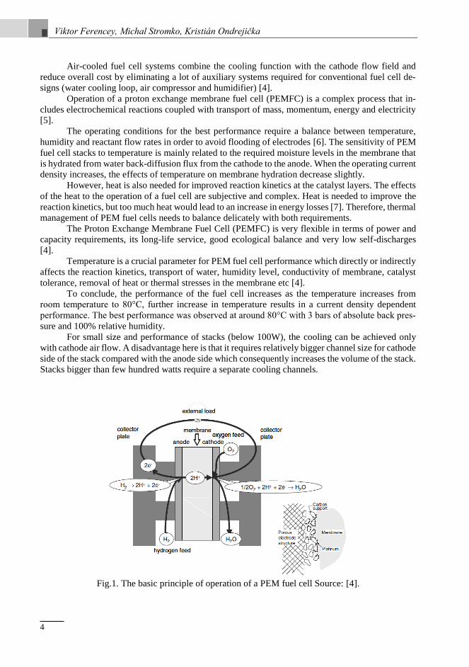
Fig.1. The basic principle of operation of a PEM fuel cell Source: [4].

Thermal Analysis of the Air-Cooled PEM Fuel Cell
5
1 Heat sources in PEMFC
The electrical performance of a PEM fuel cell dictates the generated thermal energy within the
stack. The theoretical power curve of a fuel cell can be obtained by establishing electrochemical models
based on the Nernst equation and subsequent voltage losses within the stack. Higher voltage losses at a
specified current density lead to a higher heat generation. During the operation of a PEMFC, hydrogen
molecules are supplied at the anode and split into protons and electrons. The polymeric membrane
conducts protons to the cathode while the electrons move from anode to cathode through an external load
powered by the cell. Oxygen (from air) reacts with the protons and electrons in the cathode half-cell
where water and heat are produced.
The overall reaction of a PEM fuel cell is:
H2 + ½ O2 → H2O + electrical energy + heat energy
The electrical power (𝑃𝑒𝑙) is the desired system output and the stack heat generated, or thermal
power (𝑃𝑡ℎ), of a fuel cell are linked through the actual output cell voltage (𝐸𝑐𝑒𝑙𝑙) [7],
𝑃𝑒𝑙 = 𝐸𝑐𝑒𝑙𝑙𝐼𝐹𝐶 (1)
where: 𝐼𝐹𝐶 is the current output, [A],
𝑃𝑡ℎ = (𝐸𝑁𝑒𝑟𝑛𝑠𝑡 − 𝐸𝑐𝑒𝑙𝑙)𝐼𝐹𝐶 , (2)
where: 𝐸𝑁𝑒𝑟𝑛𝑠𝑡 is the maximum achievable (reversible) voltage of a fuel cell, [V],
𝐸𝑐𝑒𝑙𝑙 = 𝐸𝑁𝑒𝑟𝑛𝑠𝑡 − 𝐸𝑎𝑐𝑡 − 𝐸𝑜ℎ𝑚 − 𝐸𝑐𝑜𝑛𝑐 , (3)
where: 𝐸𝑎𝑐𝑡 is activation, 𝐸𝑜ℎ𝑚 is ohmic, 𝐸𝑐𝑜𝑛𝑐 is mass concentration cell energy loss.
The Nernst equation for the PEM fuel cell is [4]:
𝐸𝑁𝑒𝑟𝑛𝑠𝑡 = −∆𝐺
𝑛𝐹= −
∆𝐻 − 𝑇𝐹𝐶∆𝑆
𝑛𝐹= −1.129 −
𝑅𝑇𝐹𝐶
𝑛𝐹 [𝑙𝑛(𝑝𝐻2) +
1
2𝑙𝑛(𝑝𝑂2)]
(4)
where: ∆𝐻 is the free reaction enthalpy at 298 K, which is 237.3 kJ/mol, ∆𝑆 is the reaction entropy at
298 K which is 163.33 J/(K.mol) [7], 𝑛 is the number of moles of electron transferred in the fuel cells
reaction, 𝐹 stands for Faradays constant (96,485 C/mol), 𝑇𝐹𝐶 is the fuel cell operating temperature,
usually in the range of 50 °C–100 °C, 𝑝𝐻2 is the supply pressure of the hydrogen reactant into the stack
[atm], 𝑝𝑂2 is the partial pressure of oxygen supply which is 0.21 atm for an intake of air at 1 atm [7].
1.1 Cell energy losses
The main energy loss is contributed by the activation over voltage which is the energy loss due
to the activation of electrochemical reactions at the anode and cathode. Activation losses are caused by
the slow onset of both anode and cathode reactions. Activation losses increase with current density and
can be expressed using the Tafel equation [4].

Viktor Ferencey, Michal Stromko, Kristián Ondrejička
6
𝐸𝑎𝑐𝑡 = 𝑅𝑇𝐹𝐶
𝑛𝐹 ln (
𝑖𝐹𝐶
𝑖𝑜
) , (5)
where: 𝑅 is the universal gas constant, [J/(K.kg)], 𝑇𝐹𝐶 is actual cell temperature [K], 𝑖𝐹𝐶 is generated
current density, [A/cm2], 𝑖𝑜 is a current density at electrode equilibrium [A/cm2].
The second type of energy loss is Ohmic loss contributed by the resistance to charge flow within
the cell and can be represented using Ohm's law [4].
𝐸𝑜ℎ𝑚 = 𝐼𝐹𝐶(𝑅𝑒𝑙𝑒𝑐𝑡𝑟𝑜𝑑𝑒𝑠 + 𝑅𝑚𝑒𝑚𝑏𝑟𝑎𝑛𝑒) (6)
where: 𝑅𝑒𝑙𝑒𝑐𝑡𝑟𝑜𝑑𝑒𝑠 is resistance of electrodes (resists electron flow), [Ω], 𝑅𝑚𝑒𝑚𝑏𝑟𝑎𝑛𝑒 is resistance of
membrane (resistance to proton flow through the membrane), [Ω].
The conductivity of the electrodes decreases with increasing temperature of the FC. With the
increase of the temperature, the resistance of the membrane decreases. The resistance of the membrane
dominates over the resistance of electrodes. The membrane resistance can be determined from the
following relationship [5]:
𝑅𝑚𝑒𝑚𝑏𝑟𝑎𝑛𝑒 = 𝑟𝑚 𝐿𝑚
𝐴
(7)
where: 𝑟𝑚 is the specific resistivity of the membrane to electron flow, [Ω.cm], 𝐿𝑚 is the thickness of the
membrane, [cm], 𝐴 is the active area of the PEM fuel cell, [cm2].
The concentration losses can be calculated by
𝐸𝑐𝑜𝑛𝑐 = 𝑅𝑇𝐹𝐶
𝑛𝐹ln (
𝑖𝐿
𝑖𝐿 − 𝑖𝐹𝐶
) (8)
where: 𝑖𝐿 is the maximum current density of the FC, [A/cm2], 𝑖𝐹𝐶 is the actual current density, [A/cm2].
The voltage values at a certain current density can be obtained by measuring the polarization
curve of the PEM fuel cell. These values serve as an input in simulation model based on equation (5),
(6), (7) and (8). The simulation model was created in MATLAB.
As the values obtained show, activation losses have the biggest influence on the output voltage
of the PEM fuel cell. It is possible to decrease these values by increasing the charge transfer coefficient
α, increasing the kinetics of electrode reactions, increasing exchange current density i0, and by decreasing
partial pressures and temperatures of reaction gases.
Concentration losses at a high current density have a significant influence. These losses can be
limited by maintaining the consumption rate of reaction gases under the value of diffusion coefficient D.
The diffusion coefficient defines the rate of movement as the substance diffuses into the environment,
the movement being a response to the concentration gradient in the medium in which the substance is.
In order to achieve this condition, it is necessary to change the geometry of cells or decrease current
density. Last but not least, there are also ohmic losses which grow almost linearly with increasing current
density. However, limiting ohmic losses is more complicated since they can be limited only by using
materials with lower electrical resistance. Here the reaction rate of reaction gases must be taken into
consideration when using different material as it can have a significant influence on increasing other
voltage losses.

Thermal Analysis of the Air-Cooled PEM Fuel Cell
7
After calculating individual voltage losses, the figures are used to determine the resulting PEM
fuel cell voltage so that the gradual change of generated voltage under the influence of individual losses
can be seen. shows the effect of individual voltage losses on generated voltage.
The significant voltage decrease at low current density is caused both by internal currents and by
fuel transfer from cathode to anode. These losses are a result of short circuit in electrolyte and transfer of
reactants through electrolyte. Although the electrolyte of fuel cell serves as a transfer of ions in the first
place, it is not entirely isolated from electrones and will therefore be always able to let a very small
amount of electrones through. This ability presents a net loss against/towards an outer circuit. In a real
fuel cell, the difusion process will cause that some of the reactants will move from one electrode to
another one through electrolyte where it will react without electrone transfer through the external circuit.
(Fig.2) shows four dependences of output voltage EFC as a function of current load IFC in
measured Horizon H-5000 PEM fuel cell. Individual voltage losses are gradually added to the
polarization curve of the ideal (Nernst) output voltage ENernst.
The polarization curve marked as ENernst shows the progress of ideal (Nernst) output voltage. The
curve marked as En_akt points to the progress of output voltage taking activation losses Eact into
consideration. The curve marked as En_act_conc shows output voltage polarization curve including
activation Eact and concentration Econc losses. The polarization curve marked as Ecell represents the
measured values of the PEM fuel cell output voltage.
Table 1. Comparison of output voltage values when considering individual losses
at different current density values.
In order to compare the changes of output voltage, three current load values were chosen in (Tab.
1). Low current load IFC_L equals 0.35 [A], medium current load IFC_M equals 33.41 [A] and high current
load IFC_H equals 70 [A]. (Fig.2) also pictures maximum current load of Horizon H-5000 PEM fuel cell.
It is the so called maximum current density which is characterized by insufficient amount of reaction
gases on the surface of the catalyst.
Parameter ENernst [V] En_akt [V] En_akt_conc [V] Ecell [V]
IFC_L 142.56 107.9 107.4 107.3
IFC_M 142.56 102.7 100.3 94.3
IFC_H 142.56 101.9 85.8 71.8
Fig.2. Effect of individual voltage losses on value of the resulting generated voltage.

Viktor Ferencey, Michal Stromko, Kristián Ondrejička
8
Every fuel cell has a maximum of current density called as limiting current density of FC. The
limit of this values is 76.93 [A] when measuring on Horizon H-5000 PEM fuel cell.
1.2 Heat generation
All the chemical energy that we have available in a fuel cannot be converted into useful work
(electrical energy) because of the enthalpy (entropy) change during a chemical reaction. The heat
generated within fuel cells is assumed to be the heat generated mainly at the electrochemical reaction
sites of the cathodes. Generally, to determine the amount of heat produced by a fuel cell, an energy
balance for a fuel cell stack can be provided:
∑ 𝐻𝑖,𝑖𝑛𝑖 = ∑ 𝐻𝑖,𝑜𝑢𝑡 𝑖 + 𝑃𝑒𝑙 + �̇�𝑔𝑒𝑛, (9)
or:
�̇�𝑔𝑒𝑛 − ∆𝐻𝑖 + 𝑃𝑒𝑙 = 0, (10)
where: 𝐻𝑖,𝑖𝑛, 𝐻𝑖,𝑜𝑢𝑡 are the enthalpies of reactants and products [kJ/kmol], 𝑃𝑒𝑙 is the electrical power
generated by the fuel cell [W], �̇�𝑔𝑒𝑛 is heat generated by the fuel cell, [W].
The amount of heat generated can be estimated using the simplified relations based on the energy
balance of the system and depending on the state of water formed [7]:
𝐼𝐹𝐶
𝑛𝐹 𝐻𝑢 𝑛𝑐𝑒𝑙𝑙 = 𝐼𝐹𝐶 𝐸𝑐𝑒𝑙𝑙 𝑛𝑐𝑒𝑙𝑙 + �̇�𝑔𝑒𝑛, (11)
where: 𝐻𝑢 is low heating value of hydrogen [kJ/kg].
If the water exists as vapor at room temperature, then the 𝐸𝑁𝑒𝑟𝑛𝑠𝑡 voltage is 1.254 [V] and the
stack thermal power 𝑃𝑡ℎ is dependent on the current produced and cell voltage [5]:
�̇�𝑔𝑒𝑛 = 𝑃𝑡ℎ = (𝐸𝑁𝑒𝑟𝑛𝑠𝑡 − 𝐸𝑐𝑒𝑙𝑙) 𝐼𝐹𝐶 𝑛𝑐𝑒𝑙𝑙 (12)
A fuel cell stack may dissipate its heat energy by internal as well as external mechanisms. Internal
heat removal by the cathode fluid stream is more significant than the anode fluid stream as the exothermic
reactions occur at the cathode and produced water absorbs the generated heat.
A simple way to improve the performance of a fuel cell is to operate the system at its maximum
allowed temperature. At higher-temperature, the electrochemical activities increase, and the reaction
takes place at a higher rate, which in turn increases the power output. On the other hand, operating
temperature affects the maximum theoretical voltage at which a fuel cell can operate. Higher temperature
corresponds to lower theoretical maximum voltage and lower theoretical efficiency. Temperature in the
cell also influences cell humidity which significantly influences membrane ionic conductivity.
Therefore, temperature has an indirect effect on the cell performance through its impact on the
membrane water content. The durability of the membrane electrolyte is another barrier for higher-
temperature operation due to performance degradation during long-term operation. Scientists analyzed
electrochemical performances as a function of the temperature distribution.

Thermal Analysis of the Air-Cooled PEM Fuel Cell
9
2 Analytical Simulation Model of PEMFC Stack
From the governing equations discussed before, an analytical zero-dimensional dynamic
simulation model was created in Matlab Simulink environment. Topological diagram of the created
simulation model can be seen in (Fig.3). The model consists of three interconnected subsystems which
are responsible for simulating electrochemical, thermodynamic and mass transport effects that occur
within the fuel cell stack. With this model, it’s possible to analyze the effects of ambient and operating
conditions on generated output power of the used fuel cell stack in steady state and transient modes of
operation [10], [11].
Fig.3. Topological diagram of PEMFC simulation model [10], [11].
Input parameters of the model:
𝐼𝑟𝑒𝑓 – load current (reference current) [A]
𝑃𝐻2 – pressure of the hydrogen [atm]
𝑃𝑎𝑖𝑟 – pressure of the ambient air [atm]
𝑅𝐻𝐻2 – relative humidity of the hydrogen [%]
𝑅𝐻𝑎𝑖𝑟 – relative humidity of the ambient air [%]
𝑇𝑎𝑚𝑏 – temperature of the ambient air [°C]
𝑇𝑖𝑛𝑖𝑡 – initial temperature of the FCS [°C]
Output parameters of the model:
𝐸𝑐𝑒𝑙𝑙 – generated voltage of the fuel cell [V]
𝐼𝐹𝐶 – generated current of the fuel cell [A]
𝑚𝑎𝑛,𝑤,𝑔𝑑𝑙 – amount of water transferred from membrane to anode GDL [l]
𝑚𝑐𝑎𝑡,𝑤,𝑔𝑑𝑙 – amount of water transferred from membrane to cathode GDL [l]
𝑚𝑔𝑒𝑛,𝑤,𝑔𝑑𝑙 – total amount of generated water [l]
Internal parameters of the model:
𝜆 – relative water content in the membrane [-]
𝑇𝐹𝐶 – actual working temperature of the FC [°C]

Viktor Ferencey, Michal Stromko, Kristián Ondrejička
10
The following assumptions are made for the created analytical model [9], [11]: (1) The reacting
gases are considered to be ideal; (2) The temperature is same in all parts of the fuel cell stack i.e. the
effect of conduction heat transfer is neglected; (3) No pressure drops across the flow channels are
considered; (4) The flow of generated water and reacting gases through membrane is not considered; (5)
thermodynamic properties of the solid phase are constant; (6) due to relatively low temperature and
surface area exposed to radiation, the radiation heat transfer is neglected; (7) the relation between heat
generation and local current density is linear. The focus of this paper is the thermal analysis of the
PEMFC and therefore, the thermal subsystem highlighted with green color in the (Fig.3) will be further
discussed in detail.
2.1 Thermal model of PEMFC stack
The thermal model of PEM fuel cell stack describes the changes of stack temperature depending
on the ambient temperature, heat generated by occurring electrochemical reactions and the heat
dissipated from the fuel cell by active or passive cooling. (Fig.4) shows the block representation of the
PEMFC thermal model as a MISO system with corresponding inputs and outputs. The generated fuel
cell output current 𝐼𝐹𝐶 and voltage 𝐸𝑐𝑒𝑙𝑙 which are both results from electrochemical reactions, ambient
temperature 𝑇𝑎𝑚𝑏 and initial temperature of the fuel cell stack are considered as inputs to the system.
The only output of the system is the fuel cell stack actual temperature 𝑇𝐹𝐶 [10], [11].
Fig.4. Block representation of PEMFC thermal model.
The transient change in fuel cell temperature can be represented by the following first order
differential equation [8], [10], [11]:
𝑑𝑇𝐹𝐶
𝑑𝑡=
Δ�̇�
𝑀𝑠𝑡𝑎𝑐𝑘𝑐𝑠𝑡𝑎𝑐𝑘, (13)
where Δ�̇� represents a total heat flow inside the fuel cell stack [W], 𝑀𝑠𝑡𝑎𝑐𝑘 is a weight of the fuel cell
stack [kg] and 𝑐𝑠𝑡𝑎𝑐𝑘 is an average heat capacity of the fuel cell stack [J/(K.kg)].
The total heat flow of the fuel cell stack can be calculated as a difference between generated and
dissipated heat at any given time by equation [8]:
Δ�̇� = �̇�𝑔𝑒𝑛 − �̇�𝑑𝑖𝑠𝑠, (14)
where �̇�𝑔𝑒𝑛 is the generated heat flow [W] and �̇�𝑑𝑖𝑠𝑠 represents the heat dissipated from the fuel cell
stack [W].
According to the forth mentioned equation, the value of the total feat flow will be positive when
the temperature of the system is rising and negative when the temperature is decreasing. Its value can be
also considered as a global heat gradient of the system. The amount of generated heat flow �̇�𝑔𝑒𝑛 depends
on the number of exothermic and endothermic electrochemical reactions occurring during the fuel cell
operation as seen in (12), [9], [10], [11].

Thermal Analysis of the Air-Cooled PEM Fuel Cell
11
The generated heat is causing an increase in fuel cell temperature, which in long enough time can
reach values outside the operating temperature range of PEMFC. To maintain desired operating
temperature of the stack, part of generated heat must be dissipated form the stack. Dissipation of heat
from the considered air-cooled DEA PEMFC is caused by cooling system represented by cooling fan
and by natural heat transfer mechanisms, namely convection and conduction heat transfer.
The equation of dissipated heat flow can be written as [10]:
�̇�𝑑𝑖𝑠𝑠 = �̇�𝑓𝑎𝑛 + �̇�𝑛𝑎𝑡.𝑐𝑜𝑛𝑣 , (15)
where �̇�𝑓𝑎𝑛 is a heat flow dissipated by the cooling fan [W] and �̇�𝑛𝑎𝑡.𝑐𝑜𝑛𝑣 is a heat flow dissipated from
the surface of the FCS by natural convection [W]. The dissipation of heat by conduction heat transfer
mechanism is not considered for the created model.
The following expression can be written for the heat flow dissipated by the cooling fan [8], [11]:
�̇�𝑓𝑎𝑛 = �̇�𝑎𝑖𝑟𝑐𝑝,𝑎𝑖𝑟(𝑇𝑎𝑖𝑟,𝑜𝑢𝑡 − 𝑇𝑎𝑚𝑏), (16)
where �̇�𝑎𝑖𝑟 is a mass flow rate of air [kg/s], 𝑐𝑝,𝑎𝑖𝑟 is a specific heat capacity of the air [J/(K.kg)], 𝑇𝑎𝑖𝑟,𝑜𝑢𝑡
is a temperature of the air exiting the cathode channels [°C]. The mass flow rate of air is generally
dependent on stoichiometry coefficient of the air and generated output power of the FCS. Since there is
no temperature regulation implemented in the model, the air mass flow rate �̇�𝑎𝑖𝑟 will be considered
constant and its value is given by the amount of air flowing into system through the cooling fan [10],
[11]. For the used PEMFCS and other small FCS, it can be assumed that the temperature of exiting
cathode air 𝑇𝑎𝑖𝑟,𝑜𝑢𝑡 is equal to the actual fuel cell temperature 𝑇𝐹𝐶 [11].
Heat flow dissipated by means of the natural convection from the FCS surface is given by
following relation [8], [11]:
�̇�𝑛𝑎𝑡.𝑐𝑜𝑛𝑣 = 𝛼𝑐𝑜𝑛𝑣𝐴𝑠𝑡𝑎𝑐𝑘(𝑇𝑆 − 𝑇𝑎𝑚𝑏), (17)
where 𝛼𝑐𝑜𝑛𝑣 is a coefficient of convection [W/(K.m2)], 𝐴𝑠𝑡𝑎𝑐𝑘 is the outer surface area of the FCS [m2]
and 𝑇𝑆 represents the temperature of the surface area [°C], which is in considered model, equal to FCS
actual temperature 𝑇𝐹𝐶 . For laminar flow of air, the convection coefficient for heat transfer from fuel cell
stack surface to the ambient air reaches values from 5 to 10 W/(K.m2) [11].
The complete simulation model of the thermal subsystem which was created utilizing the
equations (13) – (17) can be seen in (Fig.5). Values of the required constants of the model are summarized
in (Tab.2).
3 Results and Discussion
3.1 Model validation
In order to validate the performance of the created analytical simulation model with the
experimental data obtained from real laboratory fuel cell stack, an experimental work station shown in
(Fig.6) had to be constructed. The main part of the station is a commercial air-cooled PEM fuel cell stack
Horizon H-12 which is labelled (1) in (Fig.6). Basic parameters for this FCS datasheet are shown in
(Tab.3).

Viktor Ferencey, Michal Stromko, Kristián Ondrejička
12
Second part of the station are two metal-hydride Hydrostick cartridges (2) which can hold up to
10Wh of energy each, stored in 10L of pure dry hydrogen. The cartridges are connected to the FCS via
a one-way pressure regulating valves which are used to reduce the pressure of the cartridges to FCS input
pressure of 0.5bar. To ensure the desired functionality of the work station, a commercial control unit
supplied with the FCS was replaced by control unit (4) which was created by one of our students as a
part of his diploma thesis [11].
The control unit is able to measure voltage and current of the FCS and also humidity and
temperature of the ambient air. These values are transferred to the PC (5) by a USB interface for
validation and visualization in MATLAB environment. Besides that, the control unit also generates a
load to the FCS with the use of a controlled power MOSTFET transistor. Last functions of the control
unit are the ability to short circuit the outputs of FCS and to operate the purging valve (3). The Arduino
NANO was chosen as a microprocessor for this control unit [11].
Using the described work station, we measured the polarization curve of the fuel cell stack, which
is a standard characteristic curve for the fuel cells. It represents a steady state characteristic of fuel cell
voltage degradation in the whole operating range of the generated output current [10].
Fig.5. Simulation model - thermal subsystem [10].
Table 2. Simulation parameters of the model [11].
Sign Name Value Unit
𝑀𝑠𝑡𝑎𝑐𝑘 Weight of the FCS 0.25 [kg]
𝑐𝑠𝑡𝑎𝑐𝑘 Average heat capacity of FCS 50 [J/(K.kg)]
𝐸𝑁𝑒𝑟𝑛𝑠𝑡 Theoretical (Nernst) voltage of PEMFC 1.229 [V]
�̇�𝑎𝑖𝑟 Mass flow rate of air 4 [g/s]
𝑐𝑝,𝑎𝑖𝑟 Specific heat capacity of air 1004 [J/(K.kg)]
𝑇𝑎𝑚𝑏 Temperature of ambient air 25 [°C]
𝑇𝑖𝑛𝑖𝑡 Initial temperature of FCS 25 [°C]
𝛼𝑐𝑜𝑛𝑣 Coefficient of natural convection 7 [W/(K.m2)]
𝐴𝑠𝑡𝑎𝑐𝑘 Outer surface area of FCS 42 [cm2]

Thermal Analysis of the Air-Cooled PEM Fuel Cell
13
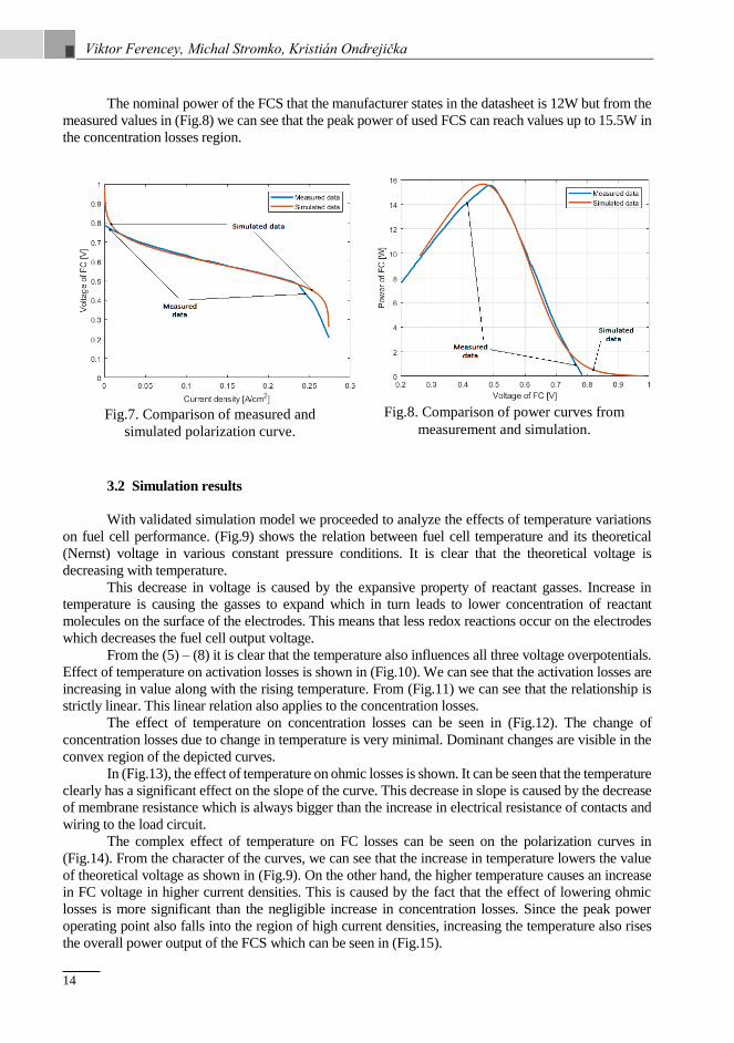
The measured data were then scaled down to represent a polarization curve for single fuel cell.
Comparison between the measured and simulated curves is displayed in (Fig.7).
The degradation occurs mainly due to polarization losses as described in 1.1. From the character
of the curves, it is clear that they corelate well in the center region where the ohmic losses are dominant.
Good fit of model in this region is important because most of fuel cells are operated in the region
of ohmic losses due to presence of their peak power point. Larger deviation is observed in the regions of
activation and mass transport losses where the model shows more pronounced logarithmic character than
the measurement.
Fig.6. Experimental work station.
Table 3. Basic parameters of Horizon H-12 [12].
Parameter Value
Number of fuel cells 13
Nominal power 12W (7.8V and 1.5A)
Maximum operating temperature 55°C
Input pressure of hydrogen 0.45 - 0.55bar
Desired hydrogen purity at least 99.995%
Membrane humidification self-hydrated
Cooling method Integrated cooling fan
Weight of the FCS 275 ± 30g
FCS dimensions 7.5 x 4.7 x 7 cm
Flow rate of the hydrogen at maximum load 0.18 l/min
Efficiency at nominal power 40%
In (Fig.8) the power curves of model and measurement are compared. The slopes of the curves
corelate very well. The main difference is visible at the peak power point where the shape of the curves
differs. This deviation is caused by different character of the polarization curves between model and
measurement in the region where the concentration losses are dominant. This can be seen in (Fig.7)
where, upon entering the concentration losses region, the measured polarization curve decreases much
faster than the simulated curve which resembles its theoretical logarithmic shape.
Viktor Ferencey, Michal Stromko, Kristián Ondrejička
14
The nominal power of the FCS that the manufacturer states in the datasheet is 12W but from the
measured values in (Fig.8) we can see that the peak power of used FCS can reach values up to 15.5W in
the concentration losses region.
3.2 Simulation results
With validated simulation model we proceeded to analyze the effects of temperature variations
on fuel cell performance. (Fig.9) shows the relation between fuel cell temperature and its theoretical
(Nernst) voltage in various constant pressure conditions. It is clear that the theoretical voltage is
decreasing with temperature.
This decrease in voltage is caused by the expansive property of reactant gasses. Increase in
temperature is causing the gasses to expand which in turn leads to lower concentration of reactant
molecules on the surface of the electrodes. This means that less redox reactions occur on the electrodes
which decreases the fuel cell output voltage.
From the (5) – (8) it is clear that the temperature also influences all three voltage overpotentials.
Effect of temperature on activation losses is shown in (Fig.10). We can see that the activation losses are
increasing in value along with the rising temperature. From (Fig.11) we can see that the relationship is
strictly linear. This linear relation also applies to the concentration losses.
The effect of temperature on concentration losses can be seen in (Fig.12). The change of
concentration losses due to change in temperature is very minimal. Dominant changes are visible in the
convex region of the depicted curves.
In (Fig.13), the effect of temperature on ohmic losses is shown. It can be seen that the temperature
clearly has a significant effect on the slope of the curve. This decrease in slope is caused by the decrease
of membrane resistance which is always bigger than the increase in electrical resistance of contacts and
wiring to the load circuit.
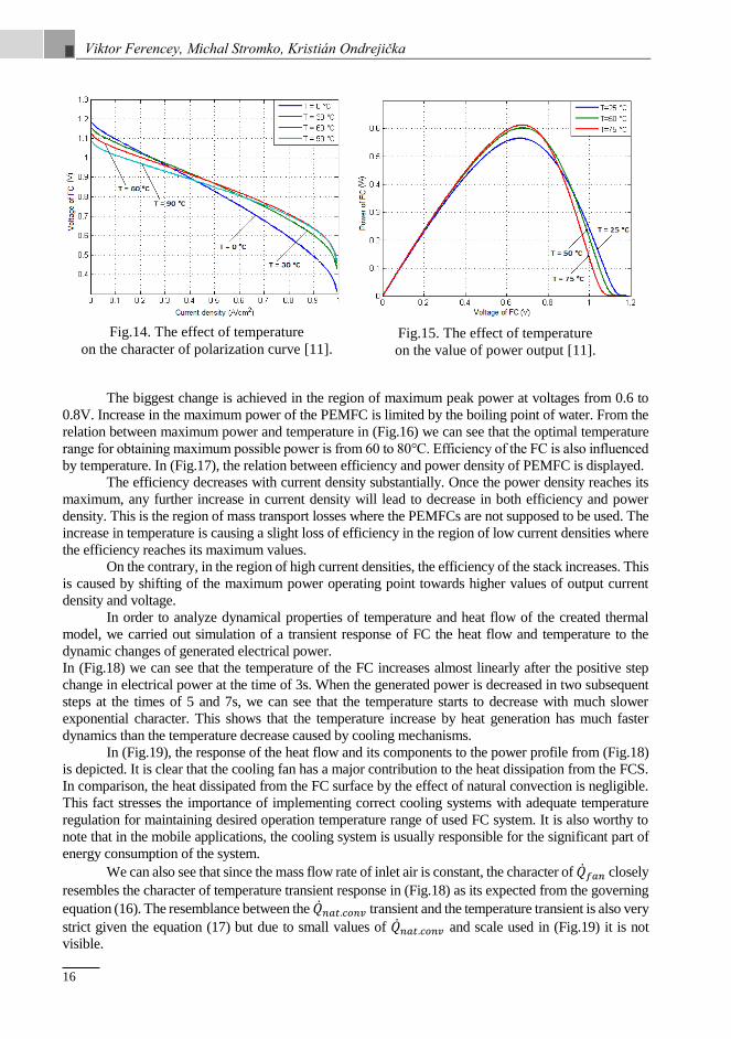
The complex effect of temperature on FC losses can be seen on the polarization curves in
(Fig.14). From the character of the curves, we can see that the increase in temperature lowers the value
of theoretical voltage as shown in (Fig.9). On the other hand, the higher temperature causes an increase
in FC voltage in higher current densities. This is caused by the fact that the effect of lowering ohmic
losses is more significant than the negligible increase in concentration losses. Since the peak power
operating point also falls into the region of high current densities, increasing the temperature also rises
the overall power output of the FCS which can be seen in (Fig.15).
Fig.7. Comparison of measured and
simulated polarization curve.
Fig.8. Comparison of power curves from
measurement and simulation.

Thermal Analysis of the Air-Cooled PEM Fuel Cell
15
Fig.13. The effect of temperature on the character of ohmic losses.
Fig.9. Theoretical voltage
as a function of temperature
at constant pressure conditions [11].
Fig.10. The effect of temperature
on the character of activation losses.
Fig.11. Relationship between activation losses
and temperature at fixed current density [11].
Fig.12. The effect of temperature on
the character of concentration losses.
Viktor Ferencey, Michal Stromko, Kristián Ondrejička
16
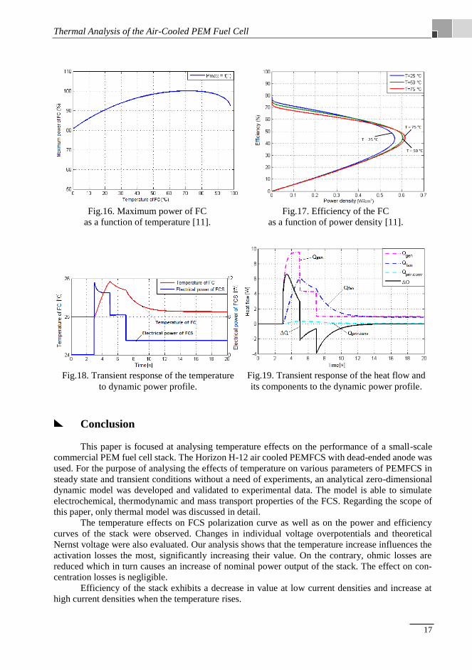
The biggest change is achieved in the region of maximum peak power at voltages from 0.6 to
0.8V. Increase in the maximum power of the PEMFC is limited by the boiling point of water. From the
relation between maximum power and temperature in (Fig.16) we can see that the optimal temperature
range for obtaining maximum possible power is from 60 to 80°C. Efficiency of the FC is also influenced
by temperature. In (Fig.17), the relation between efficiency and power density of PEMFC is displayed.
The efficiency decreases with current density substantially. Once the power density reaches its
maximum, any further increase in current density will lead to decrease in both efficiency and power
density. This is the region of mass transport losses where the PEMFCs are not supposed to be used. The
increase in temperature is causing a slight loss of efficiency in the region of low current densities where
the efficiency reaches its maximum values.
On the contrary, in the region of high current densities, the efficiency of the stack increases. This
is caused by shifting of the maximum power operating point towards higher values of output current
density and voltage.
In order to analyze dynamical properties of temperature and heat flow of the created thermal
model, we carried out simulation of a transient response of FC the heat flow and temperature to the
dynamic changes of generated electrical power.
In (Fig.18) we can see that the temperature of the FC increases almost linearly after the positive step
change in electrical power at the time of 3s. When the generated power is decreased in two subsequent
steps at the times of 5 and 7s, we can see that the temperature starts to decrease with much slower
exponential character. This shows that the temperature increase by heat generation has much faster
dynamics than the temperature decrease caused by cooling mechanisms.
In (Fig.19), the response of the heat flow and its components to the power profile from (Fig.18)
is depicted. It is clear that the cooling fan has a major contribution to the heat dissipation from the FCS.
In comparison, the heat dissipated from the FC surface by the effect of natural convection is negligible.
This fact stresses the importance of implementing correct cooling systems with adequate temperature
regulation for maintaining desired operation temperature range of used FC system. It is also worthy to
note that in the mobile applications, the cooling system is usually responsible for the significant part of
energy consumption of the system.
We can also see that since the mass flow rate of inlet air is constant, the character of �̇�𝑓𝑎𝑛 closely
resembles the character of temperature transient response in (Fig.18) as its expected from the governing
equation (16). The resemblance between the �̇�𝑛𝑎𝑡.𝑐𝑜𝑛𝑣 transient and the temperature transient is also very
strict given the equation (17) but due to small values of �̇�𝑛𝑎𝑡.𝑐𝑜𝑛𝑣 and scale used in (Fig.19) it is not
visible.
Fig.14. The effect of temperature
on the character of polarization curve [11].
Fig.15. The effect of temperature
on the value of power output [11].
Thermal Analysis of the Air-Cooled PEM Fuel Cell
17
Conclusion
This paper is focused at analysing temperature effects on the performance of a small-scale
commercial PEM fuel cell stack. The Horizon H-12 air cooled PEMFCS with dead-ended anode was
used. For the purpose of analysing the effects of temperature on various parameters of PEMFCS in
steady state and transient conditions without a need of experiments, an analytical zero-dimensional
dynamic model was developed and validated to experimental data. The model is able to simulate
electrochemical, thermodynamic and mass transport properties of the FCS. Regarding the scope of
this paper, only thermal model was discussed in detail.
The temperature effects on FCS polarization curve as well as on the power and efficiency
curves of the stack were observed. Changes in individual voltage overpotentials and theoretical
Nernst voltage were also evaluated. Our analysis shows that the temperature increase influences the
activation losses the most, significantly increasing their value. On the contrary, ohmic losses are
reduced which in turn causes an increase of nominal power output of the stack. The effect on con-
centration losses is negligible.
Efficiency of the stack exhibits a decrease in value at low current densities and increase at
high current densities when the temperature rises.
Fig.16. Maximum power of FC
as a function of temperature [11].
Fig.17. Efficiency of the FC
as a function of power density [11].
Fig.18. Transient response of the temperature
to dynamic power profile.
Fig.19. Transient response of the heat flow and
its components to the dynamic power profile.

Viktor Ferencey, Michal Stromko, Kristián Ondrejička
18
The maximum output power to temperature relation proved that the optimal temperature range
for obtaining maximum power for the used PEMFCS is 60-80°C as stated by literature. Dynamic
behaviour of temperature and heat flow in reaction to load variations shows the dominance of forced
convection in heat dissipation of the stack and stresses the importance of implementing auxiliary
cooling systems to maintain required operational temperature.
In our future work we will explore the influence of heat generation on water production and
humidity inside the FCS which are highly interconnected effects. This intention requires considera-
tion of the following aspects:
In addition to supplying the reactants to the fuel cell stack, the fuel cell system must also take care of the fuel cell by products – water and heat.
Water is essential for proton transport across the polymer membrane. Water must be col-lected at the fuel cell exhaust for reuse.
On a system level, including hydrogen and oxygen storage tanks, the mass of the system does not change, that is, hydrogen and oxygen are converted to water.
The same water may be used for humidification and to remove the heat from the stack. Heat is discharged from the system through a radiator or a liquid heat exchanger.
References
[1] KAMARUDIN S.K., DAUD W.R.W, YAAKUB Z., ANUAR W., YUSUF N.N.A.N. and MISRON Z.,
Synthesis and optimatization of future hydrogen energy infrastructure planning in Peninsular Malaysia,
in Int. J. Hydrogen Energy, 2009, 34, 2077-88.
[2] SQUADRITO G., BARBERA O., GIACOPPO G., URBANI F. and PASSALACQUA E., Polymer
electrolyte fuel cell stack research and development, in Int. J. Hydrogen Energy, 2008, 33, 1941-6
[3] BASCHUK J. and LI X., Comprehensive, consistent and systematic mathematical model of PEM fuel
cells, in Appl. Energy, 2009, 86, 181-93.
[4] BARBIR F., PEM Fuel Cells – Theory and Practice, Elsevier – Academic press, 2005, ISBN 978-0-12-
078142-3.
[5] LARMINIE J. and LOWRY J., Electric Vehicle Technology Explained, John Willey & Sons, Ltd, 2003,
ISBN 0-470-85163-5.
[6] MILLERA M. and BAZYLAKA A., A review of polymer electrolyte membrane fuel cell stack testing,
in J. Power Sources 2011, 196, 601-13.
[7] MOHAMED W.A. and ATAN R., Experimental thermal analysis on air cooling for Polymer Electrolyte
Membrane fuel cells, in Int. J. Hydrogen Energy, 2015, 40, 10605-10626.
[8] LISO V., NIELSEN M. P., KÆR S. K. and MORTENSEN H. H., Thermal modeling and temperature
control of a PEM fuel cell system for forklift applications, in International Journal of Hydrogen Energy,
Elsevier, 2014, pp. 8410-8420
[9] SHAHSAVARI S., DESOUZA A., BAHRAMI M. and KJEANG E., Thermal analysis of air-cooled
PEM fuel cells, in International Journal of Hydrogen Energy, Elsevier, 2012, pp. 18261-18271
[10] FERENCEY V., Sources and reservoirs of electrical energy for mobile means (sk. Zdroje a zásobníky
elektrickej energie pre mobilné prostriedky), Slovakia: STU Bratislava, 1st ed., 2016, pp. 76-110, ISBN:
978-80-89597-51-2
[11] GALOVIČ M., PEM fuel cell power control, Diploma thesis, Slovakia: FEI STU Bratislava, 2015, pp.
27-29, 35-53, 63-68
[12] HORIZON FUEL CELL TECHNOLOGIES, Horizon H-12 Fuel Cell Stack User Manual, ver. 2.4, Dec. 2011
pp. 11-12

Thermal Analysis of the Air-Cooled PEM Fuel Cell
19
Authors
Prof. Ing. Viktor Ferencey, PhD.
Department of Automotive Mechatronics
Faculty of Electrical Engineering and Information Technology
Slovak University of Technology, Bratislava, Slovakia
Ing. Michal Stromko
Department of Automotive Mechatronics
Faculty of Electrical Engineering and Information Technology
Slovak University of Technology, Bratislava, Slovakia
Ing. Kristián Ondrejička
Department of Automotive Mechatronics
Faculty of Electrical Engineering and InformationTechnology
Slovak University of Technology, Bratislava, Slovakia

Viktor Ferencey, Michal Stromko, Kristián Ondrejička
20

21
International Journal Volume 8, Number 1, July 2019
Information Technology Applications (ITA)
POWER SYSTEM FLEXIBILITY METRICS REVIEW
WITH HIGH PENETRATION
OF VARIABLE RENEWABLE GENERATION
M. Saber Eltohamy, M. Said Abdel Moteleb, Hossam Talaat,
S. Fouad Mekhemer, Walid Omran
Abstract:
Power systems face growing flexibility requirements for managing the increased penetrations from var-
iable renewable generation, VRG, like solar and wind power generation. In general, instant balance of
temporal inequalities between supply and demand can be reached by many flexibility options. However,
an accurate quantification of the flexibility needed and available in a power system is a complex task.
Accordingly, this paper introduces a review of various power system flexibility metrics that used to
quantify the flexibility. The use of these metrics varied, some of them were used to measure the flexibility
available from each conventional generator and others were used to measure the flexibility available
and needed by the power system at either the planning and operational stages but up - till - now there
is no flexibility metric that can be taken as a standard.
Keywords:
Power system flexibility, variable generation (VG), renewable energy.
ACM Computing Classification System:
Power estimation and optimisation, interconnect power issues, renewable energy.
1 Introduction
The continuous growth of VRG penetration has led to draw attention that future power sys-
tems may have not enough flexibility to deal with power ramps in both VRG and system demand.
Due to the variability and uncertainty of their output. The power system flexibility is the power sys-
tem capability to deploy its power resources to respond to net load changes, as net load is the system
demand minus VG output [1] [2]. A review of different flexibility definitions have been summarized
in (Table.1).
At low penetration of renewable energy the requested flexibility has provided by the reserve
generation and generators scheduling. As the system demand can be predicted to a large extent, short
duration load changes can be met by regulation and load following power plants, whereas the con-
tingency reserve are used for unpredicted outage of transmission line or generator. Hence with in-
creased penetration of VRG, it is necessary to do a new evaluation of the reserve required, and how
to measure or estimate the available and required flexibility in a power system. Although adequacy
of generation can be simply determined, the calculation of system flexibility is more complicated
and more detailed data will be required when compared to the adequacy calculations.
This paper reviews the different approaches of flexibility metrics studies. In which diverse
flexibility metrics were developed to assess power system flexibility in operation or planning stages
and to quantify the needed or available system flexibility.

M. Saber Eltohamy, M. Said Abdel Moteleb, Hossam Talaat, S. Fouad Mekhemer, Walid Omran
22
Table 1. List of Flexibility Definitions
Flexibility Definitions
1 The power system flexibility is the power system capability to deploy its power resources to respond
to net load changes, as net load is the system demand minus VG output [1][2].
2 Flexibility is the capability of a power system to balance the rapidly variation in the output of renewable
generation and forecast errors [3].
3 System flexibility is the aggregated system generators ability in responding to the net load variation
and uncertainty [4].
4 Flexibility is the capability of controllable power components in producing or absorbing power at var-
ious rates, over diverse time scales, and under a variety of power system conditions [5].
5 The transmission system ability to maintain a desired level of reliability at acceptable operation costs
even with changes in generation scenarios [6].
6 Flexibility is adaptation of the injected and/or consumed generation in response to an external signal
such as price signal so as to provide a service within the power system. The parameters that used in
characterizing flexibility consist of the amount of power that can be modulated, the duration, the rate
of change, the location etc. [7].
7 The power system ability for responding to changes in electricity in both supply and demand [8].
8 System flexibility describes its ability for accommodating the increasing performance levels at insig-
nificant extra expense for any timescale [9].
9 Flexibility is the capability of the system to react to a variety of unclear future conditions by going in
an elective direction inside satisfactory cost limit and time window [10].
10 A power system is flexible if it can inside limits reacts quickly to vast changes in demand and supply,
both scheduled and unexpected fluctuations and events, sloping down generation once demand de-
creases, and upwards once it increases [11].
11 A resource’s ability, regardless it is a component or collection of power system components, to react to
the known and unknown changes in power system conditions at different operational stages [12].
12 Flexibility refers to the ability of the system to manage events which may cause unbalance between
electricity production and demand whereas ensuring system reliability in a financially savvy way [13].
13 In its vastest sense, system flexibility refers to the degree to which a power system can adapt to the
patterns of electricity production and demand so as to keep up the balance between them within ac-
ceptable cost. While in a narrower sense, it refers to the degree to which generation or demand can be
increased or decreased over a timescale extending from minutes to hours because of changeability,
expected or otherwise [14].
14 Flexibility is typically characterized as the likelihood of altering production and/or demand patterns in
response to an external signal such as price or activation signals in order to contribute cost-effectively
to the stability of the power system [15][16].
15 The California ISO proposes flexibility in terms of rapid ramping capacity (to be delivered in 5 minutes)
provided only from the supply side of the transmission grid, complementing the other regulatory ser-
vices [17].
16 The concept of flexibility is generalized as "The capability of a power system to adjust the variation
and uncertainty through economic deployment of available resources for a given time interval. From a
probabilistic perspective, flexibility indicates the probability that the supply of flexibility is abundant
compared to the demand during the period of concern."[18].

Power System Flexibility Metrics Review with High Penetration of Variable Renewable Generation
23
Specialized Definitions of Flexibility
17 Economic flexibility is defined as “The ability to adapt, at a small extra cost, a wide range of possible
short- term demand conditions.” [19].
18 A flexible plan is defined as “One that allows the utility to change the configuration or operation of the
system rapidly and economically in response to different market and regulatory conditions.”[20].
19 Flexibility of the System is basically a trackability measure, the capability of the aggregate resources
response to track any realization of the net load random process across the operating horizon [21] [22].
20 Operational flexibility is a power system’s ability to contain a disturbance fast enough to keep the power
system secure. The most frequent disturbances are outage of components, such as transmission line or
generator tripping, or power injection deviation, e.g., because of prediction errors [23] [24].
21 Locational flexibility is the operational flexibility accessible in the grid on a given bus. Which describes
the disturbance that could be contained by appropriate and available remedial actions at a given system
node [23].
22 The exportable flexibility is the operational flexibility in a local control area that can be utilized by
neighboring control areas. Essentially, exportable flexibility is the amount of energy reserves that can
be transmitted over the tie-lines between two adjacent areas [24].
2 Power Systems Need Flexibility
Introducing a large amount of VRG to power systems causes a lot of changes in load profile
and balancing between electricity generation and consumption. Which in contrast to the conventional
dispatchable power plants and there should be enough flexibility in the power system due to:
a) VRG is dictated by climate conditions, so it is unsure ahead of time and there are forecast
errors so specific power output is unclear until it is realized.
b) VRGs are related to specific locations depending on the existence of sustainable sources of
energy e.g., wind speed and solar irradiation, which are not associated with load centers.
c) Expansion in the establishment of VRG plants displaces dispatchable conventional gener-
ation that adjusts its output to market conditions.
d) The components failures that may happen to any of power system elements (generator,
transmission line, transformer, etc.).
Fig.1. The effect of wind power production in net load.

M. Saber Eltohamy, M. Said Abdel Moteleb, Hossam Talaat, S. Fouad Mekhemer, Walid Omran
24
(Fig.1) shows the effect of wind power generation in net load which can cause the following
effects:
i. Steeper ramps (Ramp is the rate of increment or reduction in dispatchable power generation
or demand) if the wind power decreased at the same time that demand increased.
ii. Shorter peaks periods in which conventional power generations operate fewer hours which
affecting the cost.
iii. Throughout the periods of low demand, higher wind production produces the need for
dispatchable generators that can turn their output power down to the low levels but remain available
to rapidly increase it again [25].
3 Inflexibility Impacts Power Systems
Sometimes, the explanation of the opposite meaning of a word leads to better understanding
its meaning. So, features of inflexibility probably easier to be documented than flexibility. Examples
of inflexibility in power system include:
a) Difficult balance between demand and generation, leading to deviation of frequency or
drop of loads.
b) Curtailments of VRG, which occur when power generation is not required regularly (e.g.,
at night, seasonally), mostly happen because of abundance supply and when there are transmission
limitations.
c) Some Areas that have balance violations such deviations indicate how often a power system
cannot fulfil its responsibility for balancing supply.
Examples of inflexibility in the wholesale markets of power:
a) The negative prices that indicate many forms of inflexibility which include conventional
power generation which could not decrease their output, load demand which unable to utilize the
surplus power generation, excess of the renewable generation, and constrained transmission lines
ability for balancing generation and demand and to transfer power over more extensive geographic
areas. Nevertheless, negative prices sometimes happen without renewable generation in systems but
it significantly increases with increasing penetration of renewable generation.
b) Instability in prices, make prices swing between low and high, which can be a sign of
restricted capacity of transmission lines, inadequate ramping availability, quick response, and peak
power plants, and restricted demand side response [25].
4 Flexibility and Generation Adequacy
It is important to know the difference between power system flexibility and generation adequacy,
generation adequacy metrics such as well-being analysis [26] [27] [28], loss of load expectation
(LOLE) [29] [30], the expected energy not served (EENS), where power system flexibility was in-
troduced to complement the traditional capacity adequacy for the power system. The difference be-
tween the two concepts is illustrated in (Table 2) [31].

Power System Flexibility Metrics Review with High Penetration of Variable Renewable Generation
25
Table 2. The difference between flexibility and generation adequacy
Generation Adequacy System Flexibility
System demand profile used for adequacy cal-
culations is relatively predictable.
High uncertainty degree surrounds the requirements for
flexibility.
Generation Adequacy is a function of:
a) Aggregated generators’s capacity available
in the system.
b) The forced outage rate of each resource.
c) Yearly peak load hours.
Flexibility of the system affected by several other issues:
a) The generating resources in the system.
b) The availability of each resource and its ramp rate.
c) The frequency of net load ramps, magnitude and dura-
tion.
d) Prediction of variations in net load.
e) The interconnection between alternative systems.
f) The existence of storage energy systems.
g) Demand side response, DSR, availability.
h) The arrangements of market in place.
i) The strategies of reserve provision.
j) Flexibility requirements varies according to the stud-
ied time horizon.
k) Flexibility resources also depend on the time horizon
to be studied.
Generation resources used only to provide
capacity adequacy.
Generation resources used to provide both capacity ade-
quacy and system flexibility.
5 Flexibility Metrics and Assessment Methods
Flexibility metrics have been developed by those concerned with real-time operations and
the others interested in long-term planning. However, it is a complex task to accurately quantify the
flexibility requirements for a VRG-based power systems. Flexibility metrics were utilized for the
following objectives:
1. Metrics measure the system’s flexibility requirements.
2. Metrics measure the resource flexibility available.
3. Metrics measure the flexibility of the overall system including operation constraints and
transmission lines constraints.
In [10] [32], the authors identified four elements as the determinants of flexibility which are
time, uncertainty, action and cost. Flexibility was measured for power system planning as large var-
iation range in the uncertainty within which the power system remains feasible under a certain time
of response and cost threshold divided by the target uncertainty range the system intended to accom-
modate which depended on decision makers’ risk preference with taking into consideration transmis-
sion line network and constraints of system operation.
flexibility =
𝑡ℎ𝑒 𝑙𝑎𝑟𝑔𝑒𝑠𝑡 𝑣𝑎𝑟𝑖𝑎𝑡𝑖𝑜𝑛 𝑟𝑎𝑛𝑔𝑒 𝑜𝑓 𝑢𝑛𝑐𝑒𝑟𝑡𝑎𝑖𝑛𝑡𝑦𝑡ℎ𝑒 𝑠𝑦𝑠𝑡𝑒𝑚 𝑐𝑎𝑛 𝑎𝑐𝑐𝑜𝑚𝑚𝑜𝑑𝑎𝑡𝑒
𝑡ℎ𝑒 𝑡𝑎𝑟𝑔𝑒𝑡 𝑣𝑎𝑟𝑖𝑎𝑡𝑖𝑜𝑛 𝑟𝑎𝑛𝑔𝑒 𝑜𝑓 𝑢𝑛𝑐𝑒𝑟𝑡𝑎𝑖𝑛𝑡𝑦𝑡ℎ𝑒 𝑠𝑦𝑠𝑡𝑒𝑚 𝑎𝑖𝑚 𝑡𝑜 𝑎𝑐𝑐𝑜𝑚𝑚𝑜𝑑𝑎𝑡𝑒
(1)

M. Saber Eltohamy, M. Said Abdel Moteleb, Hossam Talaat, S. Fouad Mekhemer, Walid Omran
26
The power system operational flexibility was quantified and visualized in [33]. Where four parame-
ters were used: power capacity (𝜋), ramp-rate (𝜌), energy capacity (∈) and duration of the ramp (𝛿).
Operational flexibility was described as the set-points of all possible operations that constrained by
the three parameters 𝜌𝑚𝑎𝑥± , 𝜋𝑚𝑎𝑥
± and 𝜖𝑚𝑎𝑥 ± , the signs of +/- denoted for power upward and down-
ward. The relations between the individual parameters exhibit the dynamics of the so-called double
integrator where, the integration of ramp-rate 𝜌 (MW/min) gives the energy capacity ∈ (MWh),
which is the integration of power capacity 𝜋 (MW). For a power system unit (i), the three parameters
span the flexibility cube, see (Fig.2).
Where, 𝜌𝑚𝑎𝑥+ , 𝜌𝑚𝑎𝑥
− , 𝜋𝑚𝑎𝑥+ , 𝜋𝑚𝑎𝑥
− , 𝜖𝑚𝑎𝑥+ and 𝜖𝑚𝑎𝑥
− shaped the edges of the cube.
Fig.2. The cube of flexibility of a generic power system unit
with maximum available operational flexibility.
According to the authors, aggregating different units in a power system result in increasing
flexibility capability of the sum because their individual parameters of flexibility are added. For ex-
ample, a slow dynamic unit like thermal or hydro power plant which characterized by low 𝜌, high 𝜋
and ∈ constrained by fuel provision is operated with a highly dynamic unit of energy storage like a
fly-wheel that characterized by high 𝜌, low 𝜋 and limited or small ∈, see (Fig.3).
{𝜌, 𝜋, 𝜖}𝑎𝑔𝑔 = {𝜌, 𝜋, 𝜖}𝑠𝑙𝑜𝑤+{𝜌, 𝜋, 𝜖}𝑓𝑎𝑠𝑡 (2)
The overall operational flexibility provided by a pool of different units obtained by the sum-
mation of their flexibility volumes, i.e. the addition of their flexibility parameters.
𝜌𝑎𝑔𝑔+ = ∑ 𝜌𝑖
+ ,
𝑖
𝜌𝑎𝑔𝑔− = ∑ 𝜌𝑖
−
𝑖
(3)

Power System Flexibility Metrics Review with High Penetration of Variable Renewable Generation
27
𝜋𝑎𝑔𝑔+ = ∑ 𝜋𝑖
+ ,
𝑖
𝜋𝑎𝑔𝑔− = ∑ 𝜋𝑖
−
𝑖
𝜖𝑎𝑔𝑔+ = ∑ 𝜖𝑖
+ ,
𝑖
𝜖𝑎𝑔𝑔− = ∑ 𝜖𝑖
−
𝑖
Fig.3. Collecting flexibility through power system units pooling.
In operation, the available flexibility in any power system should be at any case as that needed
to mitigate an expected worst-case disturbance, see (Fig.4a). This condition is not only for the aver-
age but also for every time-step. The previous condition was illustrated by using figures, when the
required flexibility cube fitted well into the available flexibility cube as in (Fig.4b). For power system
accommodation to events that cause disturbance, the volume of the flexibility available should enve-
lope the volume of the required flexibility. If not, there is at least one of the flexibility parameters
axes lacking flexibility and the power system could not completely accommodate the disturbance
events. Mathematically, the next conditions should be verified:
𝜌𝑛𝑒𝑒𝑑𝑒𝑑+ ≤ 𝜌𝑎𝑣𝑎𝑖𝑙𝑎𝑏𝑙𝑒
+ , 𝜌𝑛𝑒𝑒𝑑𝑒𝑑− ≤ 𝜌𝑎𝑣𝑎𝑖𝑙𝑎𝑏𝑙𝑒
−
𝜋𝑛𝑒𝑒𝑑𝑒𝑑+ ≤ 𝜋𝑎𝑣𝑎𝑖𝑙𝑎𝑏𝑙𝑒
+ , 𝜋𝑛𝑒𝑒𝑑𝑒𝑑− ≤ 𝜋𝑎𝑣𝑎𝑖𝑙𝑎𝑏𝑙𝑒
−
𝜖𝑛𝑒𝑒𝑑𝑒𝑑+ ≤ 𝜖𝑎𝑣𝑎𝑖𝑙𝑎𝑏𝑙𝑒
+ , 𝜖𝑛𝑒𝑒𝑑𝑒𝑑− ≤ 𝜖𝑎𝑣𝑎𝑖𝑙𝑎𝑏𝑙𝑒
−
(4)

M. Saber Eltohamy, M. Said Abdel Moteleb, Hossam Talaat, S. Fouad Mekhemer, Walid Omran
28
(a) (b)
Fig.4. The flexibility needed versus that available during operation.
(a) Comparison. (b) The required condition for robust operation of the power system.
The authors in [34] proposed two “offline” indexes, the first offline index called normalized
flexibility index, NFI, used in evaluation the capability of individual generating units and the ability
of a mixture of generating units in providing the requested flexibility. The contribution of a genera-
tion unit to the generation mix's flexibility was determined by comparison its flexibility index to the
entire system's flexibility index. The flexibility index of the individual generator (i) was given by:
flex(i) =
12
[P𝑚𝑎𝑥(𝑖)–P𝑚𝑖𝑛(i)]+12
[Ramp(i).∆t]
P𝑚𝑎𝑥(𝑖),∀i ∈ A (5)
Where, flex(i) is positive and less than one, Pmin(i), Pmax(i) referred to minimum and maximum power
output from generator i and average value's ramp up and down denoted by 1/2 Ramp (i).
The flexibility index of the entire system (FLEX𝐴) was then determined as the sum of the
individual generator flexibility indices ( flex(i)) multiplied by a weighting factor. The weighting
factor was taken as each individual generator's capacity contribution. Therefore the flexibility of the
entire system was calculated by the following equation:
FLEX𝐴 = ∑ [ P𝑚𝑎𝑥(𝑖)
∑ P𝑚𝑎𝑥(𝑖)𝑖∈𝐴
× flex(i) ], ∀i ∈ A𝑖∈𝐴
(6)
If the flexibility index of a certain resource was greater than that of the entire system, this
resource in this system was classified as flexible. While, those power resources which were had a
flexibility index lesser than the flexibility index of the system were inflexible resources. This classi-
fication of thermal generation units as flexible or none was restricted on the studied system and
changed from system to system. This index can be utilized in comparing flexibility of various systems
or to check the flexibility of a studied system by adding new generators without performing simula-
tion for system operation.This index is fast calculated and depended only on two indicators of thermal
generation, the operating range and ramping capabilities of generator. The index is considered a sim-

Power System Flexibility Metrics Review with High Penetration of Variable Renewable Generation
29
ple method to evaluate the technical capabilities of system generators to accommodate variable re-
newable energy sources. While the operation of power system is complicated and variable, opera-
tional decisions do not affect this index. The index focuses only on flexible thermal generation
whereas the flexible demand and storage were not included in the calculations of this index.
The second offline index known as loss of wind estimation (LOWE), the index was used in
evaluating power system flexibility through the calculation of the probability of having wind curtail-
ment in the system during a year. In this index, statistical analysis were performed to calculate the
probability of net load to violate system technical thresholds which were the minimum load level and
both ramp up and down capabilities. The drawback of this index, it takes only the balancing issues
in wind curtailment and not takes into consideration the network or transmission lines constraints in
wind curtailment.
In [35], the authors presented a framework to build up a compound metric to provide a precise
flexibility evaluation within power system conventional generators. In which eight generating units’
physical characteristics were used. The eight indicators can be classified as follows:
1. Two indicators represent the operating range (OR) for each generator which are the maximum
output power (𝑃𝑚𝑎𝑥) and minimum stable output level(𝑃𝑚𝑖𝑛), measured by MW.
2. Two indicators represent the ramping capabilities for each generator, which represent the average
speed that generator increases (Ramp-Up Rate, RUR) or decreases (Ramp-Down Rate, RDR) its
output power inside the borders of operating range and measured by MW/h.
3. Four indicators relate to time which are:
The start- up time (SUT) measured by hours: which is calculated from turning on the gener-
ating unit and synchronizing it to the grid until its output power reaches 𝑃𝑚𝑖𝑛 .
The shut-down time (SDT) measured by hours: which is calculated from the time that the
output power of the generating unit drops below 𝑃𝑚𝑖𝑛 to the time when it completely stop.
Minimum up time MUT: a conventional generating unit should stay in operation for minimum
up time (MUT) after starting-up, almost for economic consideration.
Minimum down time MDT: a conventional generating unit should remain offline for a mini-
mum down time to avoid thermal stresses that decrease its lifetime.
The creation of a compound indicator was contained a sequences of stages and each step was
needed to be checked, see (Fig.5). An analytic process was applied started by indicators normaliza-
tion using min–max method, and then weights were assigned to these indicators according to their
potential impact in providing flexibility. After that the indicators were aggregated for each generator
to provide the compound flexibility index. IEEE RTS-96 test system were used for methodology
evaluation. The steps used for evolving this complex metric are explained in details as follows:
Fig.5. Sequence of steps for building up a compound flexibility metric.

M. Saber Eltohamy, M. Said Abdel Moteleb, Hossam Talaat, S. Fouad Mekhemer, Walid Omran
30
Normalization Step: Indicators of flexibility have diverse units of measurement in addition to their
disproportionate scales. Hence for the comparison simplicity and aggregation, normalization should
be done. An additional reason is to provide the direction of correlation between the individual indi-
cators and the evaluated phenomenon. For example, the SUT, SDT, MDT, MUT and 𝑃𝑚𝑖𝑛indicators
have negative correlation with the flexibility while the RUR, RDR and OR indicators have a positive
correlation. Min–max method was chosen for normalization which translates the different indicators
values to a unified range inside the interval from 0 to 1 by the following equation:
𝐼𝑗𝑖 = 𝑋𝑗𝑖 − 𝑚𝑖𝑛𝑖 (𝑋𝑗)
𝑚𝑎𝑥𝑖(𝑋𝑗) − 𝑚𝑖𝑛𝑖 (𝑋𝑗) (7)
Where, 𝑋𝑗𝑖 is the indicator j value for generator 𝑖, while 𝑚𝑖𝑛𝑖 (𝑋𝑗) and 𝑚𝑎𝑥𝑖(𝑋𝑗) are minimum and
maximum indicator𝑗 values across all generators 𝑖, 𝐼𝑗𝑖 is the normalized 𝑋𝑗𝑖 value.
Weighting step: For combining the eight flexibility indicators, weights should be given to reveal the
relative importance of each indicator in providing flexibility. The weighting methods are classified
to statistic that depend on available trusted database and participatory that rely on expert opinion. In
this study, a participatory approach was used because of lacking database. Among the participatory
techniques the analytic hierarchy process (AHP) was selected in this study. AHP is commonly uti-
lized by decision-makers when there are multi-criteria (or indicators). Where it based on comparing
each pair of indicators with regard to the objective to be achieved so as to extract weights systemat-
ically. Then a score from 1 to 9 is used to indicate the importance degree of one indicator with respect
to the other indicator. After comparing each pair of indicators, (N × N) comparison matrix is formed,
For N criteria problem; and from which each criterion weight is calculated. As the comparisons num-
ber rapidly growing with increasing the criteria number, experts sometimes become inconsistent in
their judgments. A consistency ratio (CR) to conserve integrity of the judgments is then calculated
together with the weights. The accepted value of CR is 0.10 or less; if not, the comparisons need to
be revised.
Correlation analysis step: During allocating indicators’ weights, Correlation analysis should be
done to examine if there is a high grade of correlation between any two indicators which may lead to
a double counted element in the index. For this reason, Pearson coefficient of correlation between
each pair of indicators was determined first by using the following equation:
𝑟𝑥𝑦 = ∑ (𝑥𝑖 − �̅�)(𝑦𝑖 − �̅�)𝑖
(𝑛 − 1)𝜎𝑥𝜎𝑦
(8)
Where, n is the number of indicators x and y values, �̅� , �̅� and 𝜎𝑥 , 𝜎𝑦 are their average and standard
deviations respectively. If CR is more than a predefined threshold value for a pair of indicators,
therefore the weight assigned to that pair should be revised downward in order to prevent over-rep-
resentation of the common component in these indicators. In the case of the composite flexibility
metric, if the 𝑟𝑥𝑦value was more than 0.9, the two highly correlated indicators were adjusted during
their pair-wise comparisons by decreasing the importance strength of each indicator by one level.
Aggregation step: finally; a linear summation for each normalized indicator multiplied by its relative
weight to get the generator index of flexibility as follows:
𝐹𝑙𝑒𝑥𝑖 = ∑(𝐼𝑗𝑖 × 𝑊𝑗)
𝑘
𝑗=1
(9)

Power System Flexibility Metrics Review with High Penetration of Variable Renewable Generation
31
Where, 𝑊𝑗 is the weight for indicator 𝑗 (𝑗 = 1, . . ., 𝑘) subject to ∑ 𝑤𝑗𝑗 =1 and 0≤ 𝑊𝑗 ≤1 and 𝐹𝑙𝑒𝑥𝑖 is
the flexibility index for generator 𝑖.
The drawback of this index, it does not take in to consideration the current operational state of the
generator. Where, an on line generating unit with high flexibility index could not has the capability
of providing more flexibility.
In [36], The Irish power system has wind penetration ranging from 40% to 50% of the elec-
tricity consumption. The resulting variability was managed by using a flexibility metric that utilized
in operation. The metric was used to estimate the flexibility available in the system for the upcoming
hour then comparing it to a variety values of forecasted net load so as to check whether the existing
power system resources have the capability to balance ramps in net load in case of the presence of
an estimated largely prediction error from historic wind error prediction data.
Ramping duty + Forecast Error = System Ramping Requirement
Ramping deficit = Ramping Requirement - Generator Ramping Availability
(10)
In [37], the process flexibility index was introduced by illustrating that the development goal of the
almost production processes is producing a feasible manufactured goods that meets specific quality
requirements. Between several quality features, production costs and setup time, a preferred trade-
off is made. In most applications, the multiple quality features and production costs are joined leading
to increase the difficult in getting optimum industrialized set-up. The process flexibility index was
used to evaluate the capability of both design and processing variables to achieve large changes in
the quality features. This index also used for measuring the process's capability to significantly ad-
justment the product's quality characteristics that can be used in operations planning problem. The
process flexibility metric, Cf , was expressed as "a ratio of the probability that the process will operate
within its feasible region to the probability that the process will operate within the specification
boundaries."
𝐶𝑓 =volume of feasible space
volume of Specification region =
𝑣feasible region
𝑣Specification region
(11)
A graphic representation for the index is illustrated in (Fig.6), in which 𝑦𝑖 indicating one of the qual-
ity features that has a standard preferred specification constrained by 𝑦𝑖𝑚𝑎𝑥and 𝑦𝑖
𝑚𝑖𝑛 ( 𝑦𝑖𝑚𝑎𝑥 ≤ 𝑦𝑖 ≤
𝑦𝑖𝑚𝑖𝑛) which are the maximum and minimum specification boundary.
Fig.6. Illustration of process flexibility index.

M. Saber Eltohamy, M. Said Abdel Moteleb, Hossam Talaat, S. Fouad Mekhemer, Walid Omran
32
The possible solutions for all input scenarios were represented in [38] by using the method-
ology presented in [37] in a multi-dimensional space forming the region of operating (uncut polyhe-
dron), which is not necessary in the system capacity available. Restrictions on physical variables
corresponding to the available power resources committed by a unit commitment were shaped the
outside borders of a region (cube) of constraint specification. The intersection between the operating
region and constraint specification region shaped feasibility region (cut polyhedron) which corre-
sponded to the electric potential needs that provided resources should meet. The ratio of the feasibil-
ity region measures to the operating region was termed as an index of flexibility.
Flexibility index =Volume of cut polyhedron
Volume of uncut polyhedron (12)
The index values ranged from 0 to 1, where 1 denotes the maximum flexibility. The mentioned re-
gions varied according to the studied time, giving a dynamic flexibility index evaluated over time.
The proposed index of flexibility depended on comparing the balance reserves available by unit com-
mitment and dispatching solutions to a group of VRG output scenarios and system demand. A bal-
ancing reserve solution is associated with each scenario, provided that preserves a certain level of
reliability. But, a single solution is kept for committing in advance. Obviously, one scenario's solu-
tion doesn't necessarily meet other scenarios' reliability requirements. The sum of the scenarios prob-
abilities fulfilled by the selected solution strategy defines the index of flexibility. High flexibility
index indicates that the majority of other solutions appear below the selected strategy. On the con-
trary, a solution strategy that has low index of flexibility point out that the majority of candidate
solutions are on top of that strategy, see (Fig.7).
The drawback of this metric is that it pre-supposed the calculations of a variety of unit commitment
scenarios for each period which increase the computational efforts required.
Fig.7. Comparison between high and low flexibility index for a candidate solution strategy.
In [2], the authors proposed a metric known as IRRE (insufficient ramping resource expectation)
which utilized in evaluating the flexibility of a power system in the planning stage. It was deduced
from the indicators of generation adequacy.
In this index, the ramping in net load time series, 𝑁𝐿𝑅𝑡,𝑖,+/− is determined in each time horizon then
divided to up (+) and down (-) net load ramps.

Power System Flexibility Metrics Review with High Penetration of Variable Renewable Generation
33
𝑁𝐿𝑅𝑡,𝑖 = 𝑁𝐿𝑡 − 𝑁𝐿𝑡−𝑖
1 ≤ t ≤ |NL|−i
𝑁𝐿𝑅𝑡,𝑖,+=𝑁𝐿𝑅𝑡,𝑖∀𝑁𝐿𝑅𝑡,𝑖 > 0
𝑁𝐿𝑅𝑡,𝑖,−=𝑁𝐿𝑅𝑡,𝑖∀𝑁𝐿𝑅𝑡,𝑖 < 0
(13)
Where, 𝑖 indicates the time interval, 𝑡 indicates the observation time and |NL| indicates the net load
time series length.
An offline resource provide flexibility, if its startup time, 𝑆𝑟 , is short compared to the studied
time horizon with adequate time for reaching the minimum level of stable generation. If a resource
achieves this constraint, the available upward flexibility𝑓𝑙𝑒𝑥𝑡,𝑟,𝑖,+ is determined by multiplying its
ramp up rate, 𝑅𝑅𝑟,+ , by the residual time that results from subtracting its startup time (𝑆𝑟 ) from the
studied time horizon (𝑖). For online resource, the ramp up rate, the minimum and maximum levels
of stable generation, 𝐺𝑒𝑛𝑀𝐴𝑋/𝑀𝐼𝑁,𝑟, are the necessary constraints on the available flexibility.
The upward (+) available flexibility (𝑓𝑙𝑒𝑥𝑡,𝑟,𝑖,+ ), for a resource r, over time horizon i, at
observation time t in the net load ramp time series is given by,
𝑓𝑙𝑒𝑥𝑡,𝑟,𝑖,+ = 𝑅𝑅𝑟,+ ∗ (𝑖 − (1 − 𝑂𝑛𝑙𝑖𝑛𝑒𝑡,𝑟) ∗ 𝑆𝑟)
𝑃𝑡,𝑟 + 𝑓𝑙𝑒𝑥𝑡,𝑟,𝑖,+ ≤ 𝐺𝑒𝑛𝑀𝐴𝑋,𝑟
𝑃𝑡,𝑟 + 𝑓𝑙𝑒𝑥𝑡,𝑟,𝑖,+ ∈ 𝑅\(0, 𝐺𝑒𝑛𝑀𝐼𝑁,𝑟)
(14)
Where, 𝑃𝑡,𝑟 is the resource r output power on the time of observation, t, and Online indicates the
boolean online resource variable.
Of course there is no downward flexibility 𝑓𝑙𝑒𝑥𝑡,𝑟,𝑖,−for the offline resource. The downward
flexibility available for online resources are constrained by ramp down rate (𝑅𝑅𝑟,−) and minimum
level of stable generation. The downward available flexibility from each resource r at each time of
observation, t, is calculated as follows:
𝑓𝑙𝑒𝑥𝑡,𝑟,𝑖,− = 𝑅𝑅𝑟,− ∗ 𝑖 ∗ 𝑂𝑛𝑙𝑖𝑛𝑒𝑡,𝑟
0≤ 𝑃𝑡,𝑟 − 𝑓𝑙𝑒𝑥𝑡,𝑟,𝑖,−
𝑃𝑡,𝑟 − 𝑓𝑙𝑒𝑥𝑡,𝑟,𝑖,− ∈\𝑅(0, 𝐺𝑒𝑛𝑀𝐼𝑁,𝑟)
(15)
For each resource, once both upward and downward flexibility are determined for wholly studied
time horizons, the system flexibility time series (𝑓𝑙𝑒𝑥𝑡,𝑆𝑌𝑆𝑇𝐸𝑀,𝑖,+/−) is calculated as follows:
𝑓𝑙𝑒𝑥𝑡,𝑆𝑌𝑆𝑇𝐸𝑀,𝑖,+/− = ∑ 𝑓𝑙𝑒𝑥𝑡,𝑟,𝑖,+/−
∀𝑟
(16)

M. Saber Eltohamy, M. Said Abdel Moteleb, Hossam Talaat, S. Fouad Mekhemer, Walid Omran
34
The available flexibility distribution (𝐴𝐹𝐷𝑖,+/−(𝑋) ) is deduced from 𝑓𝑙𝑒𝑥𝑡,𝑆𝑌𝑆𝑇𝐸𝑀,𝑖,+/− by
using Kaplan-Meier estimator of cumulative density functions and indicating the likelihood that a
power of X MW or lower will be available from a flexible power resource during the time hori-
zon 𝑖 [39]. From 𝐴𝐹𝐷𝑖,+/−(𝑋) , the insufficient flexibility probability for each observation time can
be calculated which represent the cumulative probability which a power system failed to meet ramp-
ing required in the net load at that observation time. In order to eliminate cases at which just enough
flexibility is available in 𝐴𝐹𝐷𝑖,+/−(𝑋), the net load ramp time series magnitude is reduced by 1MW.
Hence, the insufficient ramping resource probability (𝐼𝑅𝑅𝑃) is given by:
𝐼𝑅𝑅𝑃𝑡,𝑖,+/− = 𝐴𝐹𝐷𝑖,+/− (𝑁𝐿𝑅𝑡,𝑖,+/− − 1) (17)
After that the insufficient ramping resource expectation, 𝐼𝑅𝑅𝐸𝑖,+/− is obtained by summing the val-
ues of 𝐼𝑅𝑅𝑃𝑡,𝑖,+/− over the whole time series, 𝑇+/−, for each ramp direction as follows:
𝐼𝑅𝑅𝐸𝑖,+/− = ∑ 𝐼𝑅𝑅𝑃𝑡,𝑖,+/−
∀𝑡∈𝑇+/−
(18)
The authors in [31] studied system flexibility in planning stage. Hence some assumptions
were supposed concerning each unit operation. Such as the operation of power resources was de-
pendent on the merit order dispatch, by which electricity demand was supplied by dispatching gen-
eration units at the maximum generation from each power resource according to the incremental
marginal cost of energy. Hence, in the decisions of unit commitment, the constraints of forecast er-
rors, start-up costs and ramp rate were not included since the process was non-chronological. More-
over, the effects of transmission line network constraints were not included. Although ramps in net
load may be up or down, the upward flexibility was examined only. Because net load down ramps
could be met by several options such as ramping down the output power of generating units, reducing
excess power from renewable energy by VRG curtailment or by exporting excess power to adjacent
areas or increasing electricity consumption, While these options may be not available for ramping
up. The proposed methodology determines the periods of flexibility deficit and requires from each
flexible resource in a system such as power generators, systems of energy storage, demand side re-
sponse (DSR), and from interconnection of adjacent areas, the output power time series. The periods
of flexibility deficit were calculated as follows:
a) The average cost (AC) for every unit of generation or storage at maximum power output was
determined, and then the resources of power system were arranged in ascending order in ac-
cordance to the increase in marginal costs of full load to form the merit order supply function
[40].
AC = 𝑁𝑜𝑙𝑜𝑎𝑑𝑐𝑜𝑠𝑡 (𝑁𝐿𝐶)+𝐶𝐴𝑃𝐴𝐶𝐼𝑇𝑌∗𝑀𝑎𝑟𝑔𝑖𝑛𝑎𝑙𝐶𝑜𝑠𝑡 (𝑀𝐶)
𝐶𝐴𝑃𝐴𝐶𝐼𝑇𝑌
(19)
b) The net load time series were calculated by subtracting the output of variable generation from
the system demand at each time of observation.
NLt= system demandt- ∑ V𝐺𝑡
(20)
c) The ramps in net load (NLR) were determined in net load time series at every observation time.
NLRt,i = NLRt+i − NLRt
1 ≤ t ≤ |NL| (21)

Power System Flexibility Metrics Review with High Penetration of Variable Renewable Generation
35
d) The net load duration curve, NLDC, was formed by arranging the net load in descending order.
For system reserve provision, addition of reserve required to NLDC could be included. After
that the net load was supplied by adding resources one after the other starting with the least
cost according to the merit order and by taking into consideration minimum stable generation
level for each generator (MSG). If the scheduled operation of a generator was less than MSG,
the output power from the previous online generator was decreased by the output power re-
sulted from subtracting the scheduled output of that generator from MSG. Hence, generator
output was increased to its MSG.
e) The online power resource available flexibility, Ft,i,rOnline, was determined by calculating maxi-
mum increasing in a resource output power, for the studied time horizon constrained by the
rated power output and initial output power for that power resource at each observation time
which calculated by using the following equation:
𝐹𝑡,𝑖,𝑟𝑂𝑛𝑙𝑖𝑛𝑒 = 𝑂𝑛𝑙𝑖𝑛𝑒𝑡,𝑟 × min (𝑅𝑅𝑟 × 𝑖, 𝑅𝑎𝑡𝑒𝑑𝑐𝑎𝑝𝑎𝑐𝑖𝑡𝑦𝑟 − 𝑃𝑡,𝑟) (22)
Where, t indicated to observation time in NLDC, 𝑅𝑅𝑟 , 𝑃𝑡,𝑟 the resource, r, ramp rate and its output
power at observation time, t. The flexibility available from an offline resource if it can be synchro-
nized and start production within the selected time horizon is given by:
Ft,i,rOffline = min(RRr × (i − 𝑆𝑟), Ratedcapacityr) × (1 − Onlinet,r)
∀i ≥𝑆𝑟
(23)
To calculate the time series of the flexibility available for a power system. The summation of
both offline and online available flexibility for every power resource was added.
𝐹𝑡,𝑖𝑎𝑣𝑎𝑖𝑙𝑎𝑏𝑙𝑒 = ∑ 𝐹𝑡,𝑖,𝑟
𝑂𝑛𝑙𝑖𝑛𝑒
𝑅
𝑟=1
+ ∑ 𝐹𝑡,𝑖,𝑟𝑂𝑓𝑓𝑙𝑖𝑛𝑒
𝑅
𝑟=1
(24)
Where, R was indicated to the total power resources number.
The drawback of dispatching generators by merit order method was the exaggeration the sys-
tem's flexibility so the results in reality were sub optimal. Since the merit order commitment is non-
chronological, therefore for each time interval, the power system costs were minimized, while unit
commitment solutions take many other factors such as demand forecasting of next periods and start-
ing-up time, cost, and ramping rate for every power resource. Consequently, dispatching more ex-
pensive fast-starting, resources out-of-merit are possible for avoiding starting-up huge power re-
source that is only required for a small time period. Therefore reducing the flexibility available online
and offline with respect to the merit order method.
As a result, an improvement to the previous method for more realistic results was done by mix-
ing between merit order and economic dispatch methods. In which all power resources were dis-
patched by merit order in condition that their maximum power output were less than the net load
level. The remaining resources were dispatched for supplying the residual of net load according to
the economic dispatch method to reduce the total cost. For each power resource, the flexibility in
NLDC at every point was determined as illustrated before. A power system was considered had a
shortage in flexibility or net ramping resource deficit, PFDt,i, when NLRt,i was greater than flexibility
available 𝐹𝑡,𝑖𝑎𝑣𝑎𝑖𝑙𝑎𝑏𝑙𝑒 which equivalent to the IRRE outlined in [2].
PFDt,i = NLRt,i – 𝐹𝑡,𝑖𝑎𝑣𝑎𝑖𝑙𝑎𝑏𝑙𝑒
(25)

M. Saber Eltohamy, M. Said Abdel Moteleb, Hossam Talaat, S. Fouad Mekhemer, Walid Omran
36
Both 𝑃𝐹𝐷𝑖,+/− and 𝐼𝑅𝑅𝐸𝑖,𝑠,+/− metrics measure the system flexibility, but differ in the as-
sumptions relating to the risk level and PFDt,i is deterministic but 𝐼𝑅𝑅𝐸𝑖,+/− is a probabilistic metric.
From the previous equation, some metrics were calculated to describe the system flexibility. For
example, to exhibit the outage effect of individual units, 𝐼𝑅𝑅𝐸𝑡,𝑖𝑀𝐸𝑅𝐼𝑇/𝐻𝑌𝐵𝑅𝐼𝐷
was calculated and re-
peated for each resource removed from the group in every time horizon i.e. repeating the calculations
for (R + 1) times. For the majority of time horizons, 𝐼𝑅𝑅𝐸𝑡,𝑖𝑀𝐸𝑅𝐼𝑇/𝐻𝑌𝐵𝑅𝐼𝐷
values were higher as the
available flexibility were supplied by a smaller number of power system resources.
The drawback of this method was that the transmission line thermal limits and security constraints
were not included in calculations.
In [41], the authors presented a metric for power system planners to calculate both upward
and downward flexibility and to demonstrate the effect of transmission line networks on the flexibil-
ity by calculating maximum realizable flexibility. The upward flexibility 𝐹𝑡,𝑟+,ℎ
and the downward
flexibility 𝐹𝑡,𝑟−,ℎ
were calculated as follows:
𝐹𝑡,𝑟+,𝑖 = 𝑅𝑅𝑟
+ ∗(𝑖 − (1 − 𝑂𝑛𝑙𝑖𝑛𝑒𝑡,𝑟) ∗ 𝑆𝑟 ∗ 𝐴𝑡,𝑟)
𝑃𝑡,𝑟 + 𝐹𝑡,𝑟+,𝑖 ≤ 𝐺𝑒𝑛𝑀𝐴𝑋,𝑟
𝑃𝑡,𝑟 + 𝐹𝑡,𝑟+,𝑖 ≥ 0
(26)
𝐹𝑡,𝑟−,𝑖 = 𝑅𝑅𝑟
− ∗ 𝑖*𝑂𝑛𝑙𝑖𝑛𝑒𝑡,𝑟
𝑃𝑡,𝑖 − 𝐹𝑡,𝑟−,𝑖 ≥ 0
𝑃𝑡,𝑖 − 𝐹𝑡,𝑟−,𝑖 ≥ 𝐺𝑒𝑛𝑀𝐼𝑁,𝑟
(27)
Where, 𝐺𝑒𝑛𝑀𝐴𝑋,𝑟 , 𝐺𝑒𝑛𝑀𝐼𝑁,𝑟were indicated to the maximum and minimum generation for
every resource r respectively, the availability of each resource (r) at time (t) denoted by 𝐴𝑡,𝑟 and
𝑂𝑛𝑙𝑖𝑛𝑒𝑡,𝑟 was the binary online state variable for each resource.
If the power system network is not congested, all flexibility available from every power sys-
tem resource that scheduled for operation will be realized. But in fact the total realized flexibility
may be lower than that typically available because the flexibility estimation methods was depended
on the resource schedules alone [2]. Which had led to an overestimation of system flexibility. For
calculating realizable flexibility, an analysis for power system network should be performed by a
specialized computer programs [42] [43]. Optimization process used in calculation of maximum al-
lowable power system flexibility under a variety of conditions for all time periods. The maximum
demand that can be added to a power system and balanced by the system power resources without
breaking either the generating units or the network restrictions was defined as the maximum flexibil-
ity that can be realized for that period of time, RF. The maximum realizable flexibility for each
scenario (S) of VG output (𝑅𝐸𝑆) for each VG resource (ʋ) at a selected time horizon (i) and at every
period of time (t) was calculated. Upward realized flexibility was determined by adding the differ-
ence between total output power (P) of flexible resources at each point in time and the total power
output once the selected time horizon was passed to the alteration of VG output power during the
same time horizon as follows:

Power System Flexibility Metrics Review with High Penetration of Variable Renewable Generation
37
Maximize 𝑅𝐹𝑡,𝑖,𝑠
𝑅𝐹𝑡,𝑖,𝑠 = ∑ 𝑃𝑟,𝑡+𝑖,𝑠
𝑅
𝑟=1
− ∑ 𝑃𝑟,𝑡,𝑠
𝑅
𝑟=1
+ ∑ 𝑅𝐸𝑆ʋ,𝑡+𝑖,𝑠 − ∑ 𝑅𝐸𝑆ʋ,𝑡,𝑠
𝑉
ʋ=1
𝑉
ʋ=1
(28)
Where the number of flexible resource and the total number of them were indicated by {r,
R} respectively.
Through optimization process, net demand, and consequently, flexible power resources output power
were increased until reaching either the network or the flexibility limitations. In that case, the maxi-
mum flexibility which could be realized (RF) upwards was determined. After that, optimization pro-
cess path was altered for calculating the flexibility which could be realized downward by minimizing
realized flexibility [24]:
Minimize 𝑅𝐹𝑡,𝑖,𝑠
𝑃𝑟,𝑡+𝑖,𝑠 ≤ 𝑃𝑟,𝑡,𝑠 + 𝐹𝑟,𝑡,𝑠+,𝑖
𝑃𝑟,𝑡+𝑖,𝑠 ≤ 𝑃𝑟,𝑡,𝑠 − 𝐹𝑟,𝑡,𝑠−,𝑖
(29)
The output power was constrained by the resource's flexibility boundaries for each flexibility
power resource at the end time horizon. So, the output power change couldn’t surpass the flexibility
boundaries for either upwards or downwards, 𝐹𝑟,𝑡,𝑠+/−,𝑖
, and included resources online as well as offline.
Also network limits were included for ensuring the balance between demand and generation in addi-
tion to prevent breaching the line flow limits and preservation of power in the network.
∑ 𝐹𝑖𝑛𝑎𝑙𝐷𝑒𝑚𝑎𝑛𝑑𝑛,𝑡,𝑠 = ∑ 𝑃𝑟,𝑡+𝑖,𝑠 + ∑ 𝑅𝐸𝑆ʋ,𝑡+𝑖,𝑠
𝑉
ʋ=1
𝑅
𝑟=1
𝑁
𝑛=1
𝐹𝑖𝑛𝑎𝑙𝐷𝑒𝑚𝑎𝑛𝑑𝑛,𝑡 = ∑ 𝑃𝑙𝑎𝑛𝑡𝐴𝑡𝑁𝑜𝑑𝑒𝑛,ʋ ∗ 𝑅𝐸𝑆ʋ,𝑡+𝑖,𝑠
𝑉
ʋ=1
+ ∑ 𝑃𝑙𝑎𝑛𝑡𝐴𝑡𝑁𝑜𝑑𝑒𝑛,𝑟 ∗ 𝑃𝑟,𝑡+𝑖,𝑠
𝑅
𝑟=1
+ ∑ 𝐿𝑖𝑛𝑒𝐴𝑡𝑁𝑜𝑑𝑒𝑛,𝑙 ∗ 𝐹𝐷𝑛,𝑙
𝐿
𝑙=1
∗ 𝐿𝐹𝑙,𝑡,𝑠
𝐿𝐹𝑙𝑀𝐼𝑁 ≤ 𝐿𝐹𝑙,𝑡,𝑠 ≤ 𝐿𝐹𝑙
𝑀𝐴𝑋
𝐿𝐹𝑙,𝑡,𝑠 = −1
𝑋𝑙
∑[𝛿𝑛,𝑡,𝑠 − 𝛿𝑏,𝑡,𝑠]
𝑁
𝑛=1𝑏=1𝑏≠𝑛
(30)

M. Saber Eltohamy, M. Said Abdel Moteleb, Hossam Talaat, S. Fouad Mekhemer, Walid Omran
38
In the previous equation, {𝑛, 𝑏} indicated to the index of every bus in the system and connected buses
respectively,{𝐿𝐹𝑙,𝑡,𝑠, 𝛿, 𝐹𝐷𝑛,𝑙} indicated to the flow in line 𝑙, every bus phase angle and flow direction
on line{𝑙} at bus{𝑛} respectively. The maximum system demand that the power system able to meet
with end of time horizon was represented by 𝐹𝑖𝑛𝑎𝑙𝐷𝑒𝑚𝑎𝑛𝑑𝑛,𝑡.
Therefore the realized flexibility was estimated by considering three of varied parameters: both of
them were time dependent(𝑡, 𝑖) and the other varied parameter was the scenario of VRG output power
(𝑠).
The system requirement of flexibility was determined by net load ramp time series 𝑁𝐿𝑅𝑡,𝑖 at every
time period (𝑡) in every time horizon (𝑖), as follows:
𝑁𝐿𝑅𝑡,𝑖 = 𝑁𝐿𝑡+𝑖 − 𝑁𝐿𝑡
1≤ 𝑡 < |𝑁𝐿𝑡|
(31)
A different flexibility amount was deployed according to ramps in VRG for every scenario until the
line flow boundaries were reached. Hence, different flexibility values was estimated according to the
studied scenario and the expected values were taken at every time period to represent flexibility of
the system. The index of flexibility deficit periods (𝑃𝐹𝐷𝑠,𝑖,+/−) counted the time periods number at
which the summation of the requirements of both net load ramping (𝑁𝐿𝑅𝑡,𝑖)and contingency reserve
(𝐶𝑜𝑛𝑡𝑖𝑛𝑔𝑒𝑛𝑐𝑦𝑡) exceeded the realized flexibility (𝑅𝐹𝑡,𝑖,𝑠) for each ramp direction. Index of
𝑃𝐹𝐷𝑠,𝑖,+/− calculated for each scenario and after that the 𝑃𝐹𝐷𝑖,+/− for that time horizon and direction
was taken as the average of all scenarios values.
𝑁𝑒𝑡𝐹𝑙𝑒𝑥𝑖𝑏𝑖𝑙𝑖𝑡𝑦𝑡,𝑖,𝑠,+ = 𝑅𝐹𝑡,𝑖,𝑠 − (𝐶𝑜𝑛𝑡𝑖𝑛𝑔𝑒𝑛𝑐𝑦𝑡,+ + 𝑁𝐿𝑅𝑡,𝑖)
𝑁𝑒𝑡𝐹𝑙𝑒𝑥𝑖𝑏𝑖𝑙𝑖𝑡𝑦𝑡,𝑖,𝑠,− = 𝑁𝐿𝑅𝑡,𝑖 − 𝐶𝑜𝑛𝑡𝑖𝑛𝑔𝑒𝑛𝑐𝑦𝑡,− − 𝑅𝐹𝑡,𝑖,𝑠
𝑃𝐹𝐷𝑠,𝑖,+/− = # 𝑁𝑒𝑡𝐹𝑙𝑒𝑥𝑖𝑏𝑖𝑙𝑖𝑡𝑦𝑡,𝑖,𝑠,+/− < 0.
𝑃𝐹𝐷𝑖,+/− = 𝑀𝑒𝑎𝑛(𝑃𝐹𝐷𝑠,𝑖,+/−)
(32)
The drawback of this index was that transmission line thermal limits and security constraints
were not included in calculations.
In [44], wind and solar power that integrated with different combined penetration levels
(10%, 30%, 50% and 70% of annual demand) in Europe were discussed. A power system that has a
VRG penetration level of 70% was considered a completely renewable. The PV share was set at 20%,
40% and 60% for every level of penetration. The study showed that increasing wind/PV penetration
above 30% increased flexibility requirements. Particularly when PV contribution in the wind/PV mix
was above 20-30%. Analysis had been concluded that future requirements of flexibility in Europe
would be affected by three main factors: (1) percentage penetration of VG. (2) The VG technology
mix. (3) The system geographic distribution size.
The important element was the power ramps ∆𝑖𝑃(𝑡), which described by power variation in a studied
interval of time of (i) hours:
∆𝑖𝑃(𝑡) = 𝑝(𝑡) − 𝑝(𝑡 − 𝑖)
(33)

Power System Flexibility Metrics Review with High Penetration of Variable Renewable Generation
39
Where P(t) represented output power at time t from a spatial wind / PV unit (region or country),
t= {i+ 1,…., 8760}. Net load power ramp rates were determined for every country as function of
load, wind and PV ramp rates:
∆𝑖 𝑁𝐿(𝑡) = ∆𝑖𝐿(𝑡) − 𝛼𝛽𝐷
8760 𝜇𝑝𝑣
∆𝑖 𝑃𝑉(𝑡) − 𝛼 (1 − 𝛽)𝐷
8760 𝜇𝑊
∆𝑖 𝑊(𝑇)
(34)
In the previous equation,
∆𝑖𝑁𝐿(𝑡), ∆𝑖𝐿(𝑡), ∆𝑖𝑊(𝑡), ∆𝑖𝑃𝑉(𝑇) symbolized the power ramps in net load, load, wind and PV re-
spectively. Annual consumption was denoted by D, {W, PV} ∈ [0, 1] represented the power of wind
and PV that was normalized to the installed capacity. 𝜇𝑤, 𝜇𝑃𝑉 denoted the average power output from
wind and PV over one year. The aggregated contributions of wind / PV energy to the consumption
of annual electricity was represented by 𝛼. The aggregated PV output power contribution in the ag-
gregated contribution from wind and PV was denoted by 𝛽 as follows:
α = ∑ 𝑃𝑊𝑖𝑛𝑑(𝑡)𝑡=8760
𝑡=1 + ∑ 𝑃𝑃𝑉(𝑡)𝑡=8760𝑡=1
𝐷
β = ∑ 𝑃𝑃𝑉(𝑡)𝑡=8760
𝑡=1
∑ 𝑃𝑊𝑖𝑛𝑑(𝑡)+ ∑ 𝑃𝑃𝑉(𝑡)𝑡=8760𝑡=1
𝑡=8760𝑡=1
(35)
For performing a comparison between countries, all occurring ramps in every country were
determined as a percentage from the peak load. The system requirements of flexibility were evaluated
depending on the following factors:
(1) The level of VG penetration and the share of wind and PV in wind/PV generation,
(α,β) as choosey variables selected by decision makers.
(2) The power ramp behavioural characteristics of load, PV and wind which affected by geographic
location, the positioning of the generator and the size of the system.
(3) The correlation between ramps in VG and load and also between wind and PV ramps.
In [45], a chart of flexibility was developed which presented a simple, nontechnical means for quickly
identifying the potential of the system's flexible power resources. In which the installed capacity
percentage of five flexibility power sources including combined cycle gas turbine, hydro, pumped
hydro, combined heat and power (CHP) and interconnection relative to the peak demand were indi-
cated in the chart. However, the chart was just for indication and did not include the calculation of
overall flexibility of power system. The International Energy Agency, IEA, designed a simple com-
putation flexibility assessment tool, FAST, which utilized as a measure of requirements for flexibility
and power resources in various power system areas with different VRG penetration levels [46]. In
2014, IEA presented FAST2 which was a modified version of FAST with many timescales flexibility
assessment [47]. More data was needed by FAST2. For example, conventional unit flexibility fea-
tures, the information about DSM and interconnection. FAST2 determines maximum alteration in
the balance between generation and demand at a given instant which a power system able to meet.
In addition to the ability of computing the VRE integration level at which more flexibility is needed.
The Electric Power Research Institute, EPRI, made a framework consists of four flexibility evalua-
tion levels at various stages of power systems long-term planning process [48] [49].

M. Saber Eltohamy, M. Said Abdel Moteleb, Hossam Talaat, S. Fouad Mekhemer, Walid Omran
40
Another tool that has multi - level flexibility evaluation called InFLEXion was designed for facili-
tating decision - makers understanding of the need for flexibility of the power system. Four flexibil-
ity metrics were included in InFLEXion tool which are IRRE, PFD, expected unserved ramping
(EUR) and wellbeing assessment. EUR evaluates the total flexibility shortage magnitude rather than
duration. It determines over a certain time horizon the aggregate deficits of power ramping. Well-
being analysis used the deterministic and probabilistic indicators in diagnosing the power system
state from the following states: at risk, marginal or healthy [28]. Similarly, InFLEXion tool evaluates
the flexibility shortages magnitude and frequency over a specified time period using PFD and EUR
to decide whether the state of a power system is safe, warning, or dangerous [49].
The authors in [48] noted that the earlier studies concentrated mostly on the operating problems of
the power system and did not address the power system economic considerations of addition re-
sources of flexibility. As a result, a simulation model for stochastic production was made which
identified as REFLEX, Renewable Energy Flexibility. In which a variety of power system reliability
and flexibility indices were used in characterising the flexibility expected and shortages of adequacy
in the system. After that REFLEX evaluates the optimum investments of flexible capacity by com-
paring the addition costs of flexible resources with the improvement obtained as a result of avoided
violations of flexibility. Which assisted planners of power systems in determination of least-cost
capacity strategy to face challenges introduced by the integration of VRE in various timescales.
Power system available flexibility improvements required added costs. Several researches tried the
estimation of the flexibility provision cost which is important in selecting the optimal expansion plan
[51][52][53].
Some of power system flexibility metrics were derived from the generation adequacy indices. The
authors in [54] used the effective load carrying capability, ELCC, method that utilized in measuring
the added load which the power system able to supply with particular generator with no net change
in reliability [55][56] to suggest the effective ramping capability metric, ERC, that used in the esti-
mation of new generating unit contribution to overall power system capacity; in addition to the ap-
proximation generating unit contribution to the ramping capacity of overall power system.
In [21] [22], the authors used dynamic envelopes in characterizing the provision and requirements
of flexibility, The authors assert that by enclosing the envelope of flexibility requirement formed
through net load observations by the envelope of aggregated flexibility that shaped by flexibility
power resources sufficient power system flexibility will be achieved.
In [23], a new expression called locational flexibility was introduced for describing the power system
capability in containing a certain node disturbance. A unified framework for quantifying and com-
paring flexibility available with forecast uncertainty was presented. The presented case studies illus-
trated that flexibility was varied at diverse grid locations, it also illustrated that the use of energy
storage units and the curtailment of renewable energy could be effective means to increase flexibility
locally.
The authors in [24] presented a framework that focusing on the reserves available and the flows of
tie - line for characterizing the available operational flexibility in a power system of multi – area
which similar to the available transfer capacity, ATC, but (N-1) security criterion were taken into
consideration. The proposed approach discussed the flexible resources contribution in adjacent areas
to handle the occurred contingencies in a certain area. Hence the term “exportable flexibility” was
introduced to measure the flexibility that one area can introduce to its neighbors. If the available
flexibility is shared between different power system areas, the system can handle larger variations
which permits more integration of VRE sources. The drawbacks in the methodology were in the
calculation of the available flexibility, which was based on the assumption that the power system
demand was covered and the operational restrictions were achieved. In addition to, for validating the
methodology more examples that focusing on the generalization of the methodology to more than
two areas are required.

Power System Flexibility Metrics Review with High Penetration of Variable Renewable Generation
41
In [57], the lack of ramp probability (LORP) was proposed, like LOLP which utilized for measuring
capacity adequacy, to measure the system capability in meeting net load changes in real time. LORP
relied on the likelihood of meeting the expected next period of net load from the present generator
schedules, considering the inter temporal schedules increments of both imports and exports intercon-
nection, in order to add the positive import and negative export increases as ramp - up capacity. The
system 𝐿𝑂𝑅𝑃𝑠 for ramp up was expressed as follows:
𝐿𝑂𝑅𝑃𝑆𝑢𝑝,𝜏[𝑡] = 𝑃𝑟(∑{𝑃𝑖
𝑔[𝑡] + min(𝜏𝑅𝑖, 𝑃𝑖𝑚𝑎𝑥 − 𝑃𝑖[𝑡])} < 𝑃𝑠
𝑙
𝑖∈𝐼
[𝑡 + 𝜏]) (36)
The system 𝐿𝑂𝑅𝑃𝑠 for ramp down was expressed as follows:
𝐿𝑂𝑅𝑃𝑆𝑑𝑛,𝜏[𝑡] = 𝑃𝑟(∑{𝑃𝑖
𝑔[𝑡] + min(𝜏𝑅𝑖, 𝑃𝑖[𝑡] − 𝑃𝑖𝑚𝑖𝑛)} > 𝑃𝑠
𝑙
𝑖∈𝐼
[𝑡 + 𝜏]) (37)
Where, 𝑃𝑠𝑙[𝑡 + 𝜏] is the system net load for time step 𝜏 in the future.The zone ramp up capability,
𝑅𝐶𝑧, for 𝜏 = 1 was expressed as follows:
𝑅𝐶𝑧[𝑡] = 𝑍𝑜𝑛𝑎𝑙 𝐺𝑒𝑛𝑒𝑟𝑎𝑡𝑜𝑟 𝑅𝑎𝑚𝑝 𝑃𝑜𝑤𝑒𝑟 [𝑡] +
(𝐼𝑚𝑝𝑜𝑟𝑡[𝑡 + 1] - 𝐼𝑚𝑝𝑜𝑟𝑡[𝑡]) − (𝐸𝑥𝑝𝑜𝑟𝑡[𝑡 + 1] − 𝐸𝑥𝑝𝑜𝑟𝑡[𝑡 + 1])
(38)
The LORP for zone (𝐿𝑂𝑅𝑃𝑧) was expressed as follows:
𝐿𝑂𝑅𝑃𝑧𝑢𝑝[𝑡] = 𝑃𝑟(∑ 𝑃𝑖
𝑔[𝑡] + 𝑅𝐶𝑧[𝑡] < 𝑃𝑧𝑙
𝑖∈𝐼𝑧 [𝑡 + 𝜏]),∀𝑧
(39)
The available system flexibility of the proposed metric was computed in two-steps: (1) The network
was reduced first by considering each zone as a single bus with net injection in which all generators
and loads were connected to this bus and the transmission lines flow limits of the zone were ignored
and the tie lines between each pair of zones were aggregated to an equivalent single tie line. Then in
the first step, the generation was dispatched for meeting the net load of current time period, plus the
worst case of the following ones taking into consideration uncertainty and ramps limits. (2) In the
second step, the flow limits of the tie-lines were partially relaxed based on acceptable selected short-
term flow violation for the tie line which selected by system operator, and for the all system, a deter-
ministic optimization economic dispatch was executed with keeping the ramp capability of the zones
at the same values determined in the first step.
For current time interval and future time intervals the generator dispatch solutions were obtained
each time the two-step economic dispatch was solved. The current interval solution was implemented
whereas the future interval solutions were considered as recommended. After that the process is re-
peated by moving forward in time, and taking the updated forecast information of load and renewable
generation.
The drawback of this method, since the constraints of intra-zonal flow were not considered in step 1
of the dispatch model, all realizations of net load uncertainty were not taken into consideration by
the dispatch solution. Therefore, shortage events were reduced but not eliminated completely.
The authors in [58] [59] estimated the flexibility range for the next hours at each primary substation
node. In which, the feasible resources of flexibility that available in distribution grid that originated
from actions of flexibility (demand response, flexible distributed generation, or control of reactive

M. Saber Eltohamy, M. Said Abdel Moteleb, Hossam Talaat, S. Fouad Mekhemer, Walid Omran
42
power from the distribution system operator (DSO) assets) were informed to the transmission system
operator (TSO). The costs of activating these resources of flexibility were also considered to carry
out a cost - benefit assessment of the available actions.
The authors in [60] proposed new metrics for evaluation power system flexibility by involving the
electric vehicles (EV) into the flexible ramp market. The impact on power system reliability and
flexibility were evaluated, for both electric vehicles direct participation and by cooperation with con-
ventional generators.
In [18], the indices proposed by the authors were included: loss of flexibility probability (LOFP),
loss of flexibility duration (LOFD), loss of flexibility expectation (LOFE) and flexibility demand
shortage (FDS). The LOFP is seemed similar to LORP and IRRE but LOFP is independent with time
and LORP and IRRE are time varying. So do as LOFD and LOFE compared to PFD and ENS. The
indices have the following characteristics:
1) In case of upward flexibility, the relationship between the index and load loss is linear and so as
with RE curtailment in case of downward flexibility. The proposed flexibility indices can be deter-
mined, once the acceptable curtailment limit was determined,
2) The indices can be used with diverse options of flexibility such as units of conventional generating
and energy storage.
Conclusion
Flexibility metrics in power systems are ranged from simplicity to complexity according to
the indicators and constraints that were taken into consideration during evolving the metric and ac-
cording to whether the metric was used in operation or planning stages. Although several metrics of
flexibility and techniques of evaluation were existed, up - till - now there is no flexibility metric that
taken as a standard. Consequently, metrics are still developing.
References
[1] E. Lannoye, D. Flynn, and M. O’Malley, “The role of power system flexibility in generation
planning,” in Power and Energy Society GeneralMeeting, 2011 IEEE, july 2011, pp. 1 –6.
[2] E. Lannoye, D. Flynn, and M. O'Malley, “Evaluation of power system flexibility” IEEE. Trans.
Power Syst., vol. 27, no. 2, pp. 922–931, May 2012.
http://dx.doi.org/10.1109/TPWRS.2011.2177280.
[3] Bertsch J, Growitsch C, Lorenczik S, Nagl S. Flexibility options in European electricity markets
in high RES-E scenarios.Köln;2012.
[4] Denholm P, Hand M. Grid flexibility and storage required to achieve very high penetration of
variable renewable electricity. Energy Policy 2011;39:1817–30.
[5] Papaefthymiou, G. and Dragoon, K. (2016). Towards 100% renewable energy systems:
Uncapping power system flexibility. Energy Policy, 92, pp.69-82.
[6] Capasso, A., Falvo, M.C., Lamedica, R., Lauria, S., Scalcino, S., 2005. A new methodology for
power systems flexibility evaluation. Proc. 2005 IEEE Power Tech Conf, 1–6.

Power System Flexibility Metrics Review with High Penetration of Variable Renewable Generation
43
[7] EURELECTRIC (2014). Flexibility and aggregation: Requirements for their interaction in the
market. The Union of the Electricity Industry. Brussels, Belgium. Available online at:
http://www.eurelectric.org/media/115877/tf_bal-agr_report_final_je_ as-2014-030-0026-01-
e.pdf.
[8] Katz, J. and Cochran, J. (2015). Integrating Variable Renewable Energy into the grid: Key Issues
(Greening the Grid). National Renewable Energy Laboratory (NREL), Golden, CO, USA.
Available online at: http://www.nrel.gov/docs/fy15osti/63033.pdf.
[9] Silva, V. (2010). Value of flexibility in systems with large wind penetration. PhD thesis, Imperial
College London.
[10] Zhao, J., Zheng, T., and Litvinov, E. (2016). A unified framework for defining and measuring
flexibility in power system. IEEE Transactions on Power Systems, 31(1):339–347.79
[11] IEA (2005). Variability of wind power and other renewables. Management options and strategies.
International Energy Agency. Paris, France. Available online at: http://www.
uwig.org/iea_report_on_variability.pdf.
[12] Ela, E., Milligan, M. R., Bloom, A., Botterud, A., Townsend, A., and Levin, T. (2014).
Evolutionof wholesale electricity market design with increasing levels of renewable generation.
National Renewable Energy Laboratory (NREL). Golden, CO, USA. Available online at:
http://www.nrel.gov/docs/fy14osti/61765.pdf.
[13] Ma, J. (2012). Evaluating and planning flexibility in a sustainable power system with large wind
penetration. PhD thesis, The University of Manchester.
[14] IEA (2014). The Power of Transformation. Wind, Sun and the Economics of Power System
Flexibility. International Energy Agency. Paris, France. Available online at
https://goo.gl/hjVBWM.
[15] Villar, José, Ricardo Bessa, and Manuel Matos. "Flexibility products and markets: Literature
review." Electric Power Systems Research 154 (2018): 329-340.
[16] Rivero, E., D. Six, and H. Gerard. "Assessment of future market architectures and regulatory
frameworks for network integration of DRES–the future roles of DSOs." evolvDSO project,
Deliverable 1 (2015).
[17] Xu, Lin, and Donald Tretheway. "Flexible Ramping Products." (2012).
[18] Lu, Zongxiang, Haibo Li, and Ying Qiao. "Probabilistic flexibility evaluation for power system
planning considering its association with renewable power curtailment." IEEE Transactions on
Power Systems 33.3 (2018): 3285-3295.
[19] G. Stigler, "Production and Distribution in the Short Run," J.Political Econ., Vol. 47(3), pp. 305-
327, 1939.
[20] Benjamin F. Hobbs, Jeffrey C. Honious, Joel Bluestein,“Estimating the Flexibility of Utility
Resource Plans: An Application to Natural Gas Cofiring for SO2 Control”, IEEE Transactions on
Power Systems, Vol. 9, No. 1, February 1994, pp 167-173.
[21] Nosair, Hussam, and Franois Bouffard. "Flexibility envelopes for power system operational
planning." IEEE Transactions on Sustainable Energy 6.3 (2015): 800-809.
[22] Nosair, Hussam, and Franois Bouffard. "Reconstructing operating reserve: Flexibility for
sustainable power systems." IEEE Transactions on Sustainable Energy 6.4 (2015): 1624-1637.
[23] Bucher, Matthias A., et al. "On quantification of flexibility in power systems." PowerTech, 2015
IEEE Eindhoven. IEEE, 2015.
[24] Bucher, Matthias A., Spyridon Chatzivasileiadis, and Göran Andersson. "Managing flexibility in
multi-area power systems." IEEE Transactions on Power Systems 31.2 (2016): 1218-1226.
[25] Jaquelin Cochran et al., “Flexibility in 21st Century Power Systems” (Golden, CO: National
Renewable Energy Laboratory, May 2014).
[26] R. Billinton and G. Lian, “Composite power system health analysis using a security constrained
adequacy evaluation procedure,” IEEE Trans. Power Syst., vol. 9, pp. 936–941, May 1994.
[27] R. Billinton, R. Karki, “Application of Monte Carlo simulation to generating system well-being
analysis,” IEEE Trans. Power Syst., vol. 14, pp. 1172–1177, Aug. 1999.
[28] R. Billinton and M. Fotuhi-Firuzabad, “A basic framework for generating system operating health
analysis,” IEEE Trans. Power Syst., vol. 9, no. 3, pp. 1610–1617, Aug. 1994.
[29] G. Calabrese, “Generating reserve capacity determined by the probability method,” Trans. Amer.
Inst. Elect. Eng., vol. 66, no. 1, pp.1439–1448, Jan. 1947.

M. Saber Eltohamy, M. Said Abdel Moteleb, Hossam Talaat, S. Fouad Mekhemer, Walid Omran
44
[30] R. Billinton and R. Allan, Reliability Evaluation of Power Systems, 2nd ed. New York: Plenum,
1996.
[31] E. Lannoye, D. Flynn, and M. O'Malley, “Assessment of power system flexibility: A high-level
approach,” in Proc. 2012 IEEE Power and Energy Society General Meeting, Jul.
[32] Jinye Zhao, Tongxin Zheng, Eugene Litvinov “A Unified Framework for Defining and
Measuring Flexibility in Power System” Optimization and Equilibrium in Energy Economics
Workshop ,11 Jan. 2016.
[33] Ulbig, Andreas, and Göran Andersson. "Analyzing operational flexibility of electric power
systems." International Journal of Electrical Power & Energy Systems 72 (2015): 155-164.
[34] J. Ma et al., “Evaluating and planning flexibility in sustainable power systems,” IEEE Trans.
Sustain. Energy, vol. 4, no. 1, pp. 200–209,2013
[35] Oree, V. and Sayed Hassen, S. (2016). A composite metric for assessing flexibility available in
conventional generators of power systems. Applied Energy, 177, pp.683-691.
[36] EirGrid, “Delivering a Secure Sustainable Power System,” 2011. [Online]. Available:
http://www.eirgrid.com/media/IndustryForum(DundalkAug02011).pdf
[37] David Kazmer, David Hatch, Liang Zhu, Christoph Roser, Deepak Kapoor, “Definition and
Application of a Process Flexibility Index”, Transactions on ASME, Vol. 125, February 2003.
[38] N. Menemenlis, M. Huneault, and A. Robitaille, “Thoughts on power system flexibility
quantification for the short-term horizon,” in Power and Energy Society General Meeting, 2011
IEEE, July 2011.
[39] E. L. Kaplan and P. Meier, “Nonparametric estimation from incomplete observations,” J. Amer.
Statist. Assoc., vol. 53, no. 282, pp. 457–481, 1958.
[40] S. Stoft, Power System Economics: Designing Markets for Electricity. Wiley - IEEE Press, 2002.
[41] E. Lannoye, D. Flynn, M. O’Malley ”Transmission, Variable Generation, and Power System
Flexibility” IEEE Transactions on Power Systems, 30 (1) (2015), pp. 57-66
[42] M. Saber, F. M. A. Ghali and E. E. Abou Elzahab, "The effect of DG penetration on short circuit
currents level," 2017 Intl Conf on Advanced Control Circuits Systems (ACCS) Systems & 2017
Intl Conf on New Paradigms in Electronics & Information Technology (PEIT), Alexandria, 2017,
pp. 291-296.
[43] M. Saber, F. M. A. Ghali, and E. E. Abou Elzahab. "Proposed algorithm for DG allocation in
distribution networks." In 4th international conference on advanced control circuits and systems
accs015, Luxor, Egypt, organized by Electronics Research Institute (ERI), pp. 15-19. 2015.
[44] Huber, M., Dimkova, D. and Hamacher, T. (2014). Integration of wind and solar power in
Europe: Assessment of flexibility requirements. Energy, 69, pp.236-246.
[45] YasudaY, ArdalAR, CarliniEM, EstanqueiroA, FlynnD, Gomez-LázaroE, et al. Flexibility Chart:
Evaluation on diversity of flexibility in various areas. 12th Int. Work. Large-Scale Integr. Wind
Power into Power Syst. as well as Transm. Networks Offshore Wind Power Plants, London, UK:
2013.
[46] International Energy Agency. Harnessing variable renewables: A guide to the balancing
challenge. OECD Publishing, 2011.
[47] International Energy Agency. Grid Integration of Variable Renewables (GIVAR) Phase III. 2014.
[48] Oree, Vishwamitra, Sayed Z. Sayed Hassen, and Peter J. Fleming. "Generation expansion
planning optimisation with renewable energy integration: A review." Renewable and Sustainable
Energy Reviews 69 (2017): 790-803.
[49] EPRI. Metrics for quantifying flexibility in power system planning. 2014.
[50] Hargreaves J, Hart EK, Jones R, Olson A. REFLEX: An adapted production simulation
methodology for flexible capacity planning. IEEE Trans Power Syst 2014;30:1306–15.
[51] Milligan M, Ela E, Hodge BM, Kirby B, Lew D, Clark C, et al. Integration of variable generation,
cost-causation, and integration costs. Electr J 2011;24:51–63.
[52] IEA. The power of transformation: Wind, sun and the economics of flexible power systems.
2014.
[53] Hirth L, Ueckerdt F, Edenhofer O. Integration costs revisited - An economic framework for wind
and solar variability. Renew Energy 2015;74:925–39.
[54] Lannoye E, Milligan M, Adams J, Tuohy A, Chandler H, Flynn D, et al. Integration of variable
generation: Capacity value and evaluation of flexibility. IEEE PES Gen. Meet. PES 2010;2010.
http://dx.doi.org/10.1109/PES.2010.5589889.

Power System Flexibility Metrics Review with High Penetration of Variable Renewable Generation
45
[55] Milligan, Michael, and Kevin Porter. Determining the Capacity Value of Wind: An Updated
Survey of Methods and Implementation; Preprint. No. NREL/CP-500-43433. National
Renewable Energy Laboratory (NREL), Golden, CO., 2008.
[56] Milligan, M., and Kevin Porter. Determining the Capacity Value of Wind: A Survey of Methods
and Implementation; Preprint. No. NREL/CP-500-38062. National Renewable Energy Lab.,
Golden, CO (US), 2005.
[57] A.A. Thatte, L. Xie, A metric and market construct of inter-temporal flexibilityin time-coupled
economic dispatch, IEEE Trans. Power Syst. 31 (September (5)) (2016) 3437–3446.
[58] Heleno, M., et al. “Estimation of the flexibility range in the transmission-distribution boundary."
PowerTech, 2015 IEEE Eindhoven. IEEE, 2015.
[59] Silva, João, et al. "The challenges of estimating the impact of distributed energy resources
flexibility on the TSO/DSO boundary node operating points." Computers & Operations Research
(2017).
[60] Zhang, Bei, and Mladen Kezunovic. "Impact on power system flexibility by electric vehicle
participation in ramp market." IEEE Transactions on Smart Grid 7.3 (2016): 1285-1294.
Authors
M. Saber Eltohamy
Department of Power Electronics and Energy Conversion,
Electronics Research Institute, Cairo, Egypt
[email protected] Mohammed Saber is a Research Assistant at the Electronics Research Institute in Egypt.
He received his BSc from Faculty of Engineering at Shoubra, Benha University, and MSc from Cairo Faculty of Engineering, Cairo University, Egypt. He is a PhD student
in Ain Shams Faculty of Engineering, Ain Shams University, Egypt.
M. Said Abdel Moteleb
Department of Power Electronics and Energy Conversion,
Electronics Research Institute, Cairo, Egypt, Professor
[email protected] Mohamed Moteleb is a Professor of Power Electronics and Energy Saving at the Elec-tronics Research Institute in Egypt. He received his BSc and MSc from the Faculty of
Engineering, Cairo University, and PhD from the Faculty of Electrical Engineering and Information Technology, Slovak Technical University, Slovakia. Prof. Moteleb is one
of the leading Editors-in-Chief of the Journal of Electrical Systems and Information Technology.
Hossam Talaat
Department of Electrical Power and Machines Engineering,
Ain Shams University, Cairo, Egypt, Professor

M. Saber Eltohamy, M. Said Abdel Moteleb, Hossam Talaat, S. Fouad Mekhemer, Walid Omran
46
S. Fouad Mekhemer
Department of Electrical Power and Machines Engineering,
Ain Shams University, Cairo, Egypt, Associate Professor
Walid Omran Department of Electrical Power and Machines Engineering,
Ain Shams University, Cairo, Egypt, Associate Professor

47
International Journal Volume 8, Number 1, July 2019
Information Technology Applications (ITA)
FEATURES OF THE IMPLEMENTATION
OF TIME MANAGEMENT TECHNIQUES
IN THE PROGRAMMING LANGUAGE DART
Yakov Lvovich, Emma Lvovich
Abstract:
The purpose of this work is to develop a prototype of a mobile application, which is a tool for personal
time management, in the programming language Dart using the Flutter framework. In the course of the
work, the research of the subject area of time management techniques was carried out, according to the
results of which the methodology for implementation was chosen. Also, the research of the subject area
and the features of software and language solutions were analyzed for the implementation of the proto-
type. Application development was carried out in the high-level language Dart (SDK) using the Flutter
Framework (SDK) in the integrated development environment Android Studio. The prototype mobile
application is designed for a user with minimal skills on Android devices. The application has an intui-
tive ergonomic interface, it contains a timer tool, a description of the tool, allowing you to use the
prototype as a tool for personal time management. The mobile application is developed, the user inter-
face is designed, the information system is developed, algorithms for drawing up personal statistics are
developed.
Keywords:
Сomputer application, online store, Android, user.
ACM Computing Classification System
Distributed systems organizing principles, software functional properties,
specialized application languages
Introduction
Currently, information technology is an integral part of our lives. Modern man can not imag-
ine his day without using a smartphone, tablet or smart watch. Therefore, the development of various
mobile applications to provide users with comfortable operation of their devices is in demand [1].
Such demand creates a demand for programmers and a demand for new, simpler, more con-
venient and accessible tools for development - languages and environments.
To use the time resource most effectively, both for personal purposes and for work, you need
to use time management.
Time management is a set of knowledge, skills and abilities, thanks to which a person is able
to prioritize, accurately plan his time, thereby increasing his personal productivity in the organization
of his working time. Time management includes many different techniques.
From the analyzed techniques of time management, the method of "Pomodoro" was chosen
for implementation. It is simple, but it provides more control than the techniques with sorting tasks
by type and importance - Eisenhower Matrix or Franklin Pyramid. It is also possible to use this
technique for more effective application of such time management method as "Eat a frog first".

Yakov Lvovich, Emma Lvovich
48
Among other things, statistics on work with such a tool will be easier to implement - you do
not need to assess the effectiveness of the work done, because of the short-term method, statistics are
generated in a short time, which makes it easy to analyze the effectiveness of the methodology and
indicate progress.
Currently, there are many different applications-tools for time management technique "Po-
modoro". These applications provide all the classic features of this technique, have a simple intuitive
interface, some have the ability to configure the time intervals for work and rest, change the param-
eters of sound notifications. These solutions are mostly:
a) designed only for use on one of the platforms - either Android or IOS [2];
b) they do not have Russian localization;
c) they are paid or shareware with the presence of advertising banners.
In this paper we consider the development of an application for time management on the basis of the
language Dart.
1 Technologies Used
When implementing the application, the following technologies were used:
- Dart programming language (SDK version 3.2.0);
- Flutter framework (SDK version 1.5.4);
- Integrated Development Environment Android Studio (version 3.4);
- SQLite, a plug-in library (sqflite version 3) for creating a local database;
- Sourcetree - program for creating backup copies of working code with the ability
to roll back to previous working versions;
- draw.io - to create a visual database structure, build the architecture of a software
system, edit screen forms.
2 Dart Programming Language
Dart is a cross-platform, object-oriented, scripted, multi-paradigm functional programming
language.
Google offered Dart at the end of 2011 as a language for web development, devoid of JavaS-
cript flaws, which are associated, in particular, with the inconvenience of structuring programs when
their size goes beyond simple web applications. The main goal of this initiative was to create the
most convenient programming environment specifically designed for the development of web con-
tent [3].
Currently, Dart is used to create both simple scripts and full-featured applications. In addition
to web development with it, you can create mobile applications (using the Flutter framework), com-
mand line scripts, or server applications. Flexible compilation technology allows you to run Dart
code depending on the chosen platform and developer's according goals.
3 Mobile Application Implementation
The implementation begins with the creation of a user interface. For this prototype of the
mobile application, 2 pages were created for implementing the database and 10 pages for implement-
ing the user interface, then their functionality and structure are described.

Features of the Implementation of Time Management Techniques in The Programming...
49
1. welcome_screen.dart
Description: Welcome page of the application.
Main functions:
- Displays a random motivational quote from a list of quotes;
- carries out transition to the menu page;
Structure: The basis of the page is StatelessWidget. To implement the Random method, to
select a random quote from the List, the dart: math package is enabled and the dart_random_choice:
^ 0.0.2 dependency is added in the pubspec.yaml file (Fig.1). Similarly, libraries are connected that
are not part of the standard language set - after adding a dependency, the required library is automat-
ically downloaded and installed. The floatingActionButton button is used to go to home_screen.dart
(Fig.2).
Fig.1. List of added dependencies in the pubspec.yaml file.
2. home_screen.dart
Description: The main menu of the application.
Main functions:
- contains four main buttons for navigating through the sections of the application:
“Proceed”, “Completed”, “Statistics”, “About the Tool”;
- contains a button to add a new task from the menu;
Structure: The basis of the page is StatefulWidget. The menu is made using the Stag-
geredGridView, with the connection of the corresponding flutter_staggered_grid_view.dart package
and dependencies (Fig.1). Each menu button is an Icon wrapped in InkWell, and redirects to the
appropriate section. Use the floatingActionButton button to go to the new_task.dart page.
3. new_task.dart
Description: Form for adding a new task.
Main functions:
- adding data to the database by entering the text in the appropriate fields - “Name”
and “Description”. Selecting the priority value from the drop-down list;
- deletion of data from the database, if the record is edited;
- clean form fields, if the task has not yet been saved in the database [4];
- redirection in the menu after saving or deleting data;

Yakov Lvovich, Emma Lvovich
50
Fig.2. Navigation between application pages,
home screen: enter, statistics, completion, description.
Fig.3. Adding a new task: insert task, set priority,
Status: task succesfully completed.

Features of the Implementation of Time Management Techniques in The Programming...
51
Structure: The basis of the page is StatefulWidget. To work with dates, the package intl.dart
is included. The priority value is selected using DropdownMenuItem, the String variable is not
“High” or “Low”, but the Int is “1” or “2”, the data type is converted using the updatePriorityAsInt
function, and from the database is taken by getPriorityAsString. To capture text, use a special con-
troller TextEditingController. The following updateTitle functions are used to work with the database
- when entering data in the "Name" field, updateDescription - when entering data in the "Description"
field, _save - when you click the "Save" button, _delete - when you click the "Delete" button. The
_showAlertDialog function calls the status dialog box confirming successful saving (Fig.8) or delet-
ing data in the database or displays an error.
4. to_do_task.dart
Description: List of tasks performed.
Main functions:
- displays a list of tasks performed in accordance with the priority.
For each task is displayed:
- name;
- date of creation or editing;
- priority icon before task name. Icons.arrow_upward is red for high priority
and Icons.arrow_downward is yellow for low. Changes when editing priority.
- timer icon that redirects to the timer tool page;
- go to the edit page, with the ability to save changes or delete the task;
- the possibility of adding a new task.
Structure: The basis of the page is a StatefulWidget (Fig.4). Using the updateListView func-
tion, the task list from the database is populated in accordance with the priority. Only tasks with the
status “Executed” are displayed in the list. Each task is represented as a Card representing ListTile
with the following elements: Leading Icon, changing the color and appearance of the priority icon,
using the getPriorityColor and getPriorityIcon methods. Title displays the name of the task [5]. Sub-
title the date the task was created or modified. Trailing Icon navigates to the timer tool (Fig.5).
Clicking the ListTile navigates to the edit page of the selected task. FloatingActionButton
redirects to the new_task.dart page.
5. task_timer.dart
Description: Timer tool.
Main functions:
- displays the task on which the work is being done;
- has a form in which you can put a mark if the task is completed;
Structure: The basis of the page is StatefulWidget. Text displays the name of the selected
task. The checkbox, when clicked, changes the status of the task in the database from “Running” to
“Completed” by passing the variable through StreamController.
6. task_work_timer.dart, task_rest_timer.dart
Description: Timer for work and play.
- working timer has a duration of 25 minutes, the rest timer 5 minutes,
Timer change;
- reproduces the animation of filling the circle in accordance
with the elapsed time interval of the timer;
- displays the change of timer numbers;
- allows you to stop and resume the timer;
- fixing past tense;
Structure: (continued on page 9)

Yakov Lvovich, Emma Lvovich
52
Fig.4. Division of to_do_task.dart into widgets: set of tasks, ListTile with three elements.
Fig.5. Choosing a timer tool, right: Work timer, button Break to rest.

Features of the Implementation of Time Management Techniques in The Programming...
53
Main functions:
Fig.6. Timer for work and leisure, left: Work timer, button Break to rest,
right: Rest timer, button Work start.
Fig.7. Removing a task from the list of completed tasks.

Yakov Lvovich, Emma Lvovich
54
Fig.8. Short application instructions what to do and what button to press.
Fig.9. Statistics: Today results and Week results -
number of tasks, completed tasks, time spent, time effectivity.

Features of the Implementation of Time Management Techniques in The Programming...
55
Structure: The basis of the pages is StatefulWidget. Besides the differences in the length of
the timer, they are no different. First of all, the math package is connected and two circles are built
for animation. The first is a contour, the second fills it with a brighter gradient. The following widgets
were used to create circles and animation: AspectRatio, AnimatedBuilder, CustomPaint.
To transfer the elapsed time from the start of the timer, the streamController is used, which
allows you to send the value of a variable using stream and recognize it with the help of listen. The
time interval is stored in the String data type, which must be converted to an int using the parse
method.
7. done_task.dart
Description: List of completed tasks.
Main functions:
- displays a list of completed tasks;
- allows you to delete a task from the list;
Structure: The basis of the page is StatefulWidget. Using the updateListView function, the
list of completed tasks from the database is populated. Each task is presented in the form of a Card
representing ListTile with the following elements: Leading Icon, Title displays the name of the task,
Subtitle displays the date of creation or modification of the task. Trailing Icon allows you to delete a
task from the database. SnackBar pops up on the bottom of the screen with a notification that the task
[6, 7] was successfully deleted from the database (Fig.7).
8. statistic.dart
Description: Display statistics.
Main functions:
- displays the number of all tasks.
Structure: The basis of the page is a StatefulWidget with a text image of the statistics of
working with the tool (Fig.9).
9. how_to_use.task
Description: Short instructions for using the application.
Main functions:
- briefly explain the principle of working with the tool;
Structure: The basis of the page is StatefulWidget. PageView is used - a scrolling list of pages,
by default, i.e. scrolling goes horizontally. It has text widgets briefly describing the principle of
working with this tool (Fig.8).
User interface is then created and DB is connected. Tests are conducted during development,
due to the hot-reload function. To complete the development project, it remains to receive a release
version of the application. To do this, use the console flutter_console.bat. The command line contains
the location of the project and the corresponding flutter build apk-release command (Fig.10). The
installation process of the application is standard. The application is waiting for refinement and does
not have a digital signature, therefore, at the moment can not be downloaded to PlayMarket.
Conclusion
Flutter is a handy tool for creating user interfaces. Nevertheless, it requires a thorough
knowledge and understanding of the work of the Dart libraries. All planned functions of the applica-
tion have been implemented. Prototype testing was conducted on iOS. The prototype can be im-
proved with extended calculation of statistics and optimization of the widget tree.

Yakov Lvovich, Emma Lvovich
56
Fig.10. Application release.
References
[1] Preobrazhensky Yu. P. (2018) Information technologies used in the field of management. Bulletin
of Voronezh Institute of high technologies. № 2(25). P. 43-46.
2 Vinokurov A.V. (2019) Features of the use of reactivex technology in mobile applications for the
Android operating system. Bulletin of Voronezh Institute of high technologies. № 1(28). P. 53-57.
3 Kostrova V. N., Gusev A.V. (2018) Methods and tools for developing and evaluating the quality of
web applications. Bulletin of Voronezh Institute of high technologies. № 2(25). P. 75-78.
[4] Kamakin V. D., Lvovich I. Ya. (2018) Problems of protection of electronic documents. Bulletin of
Voronezh Institute of high technologies. № 4(27). P. 64-66.
[5] Melnikova T. V. (2016) Some features of business analyst's work in it-sphere. Modeling, optimiza-
tion and information technologies. № 1 (12). P.5.
[6] Chernikov S. Yu., Korolkov R. V. (2014) the Use of system analysis in the management of organi-
zations. Modeling, optimization and information technologies. № 2 (5). P. 16.
[7] Samoilova U. A. (2014) On some characteristics of enterprise management. Bulletin of Voronezh
Institute of high technologies. No. 12. P. 176-179.
Authors
Prof. Yakov Lvovich
Doctor of Sciences (Engineering), professor
Voronezh Institute of High Technologies
Ass. prof. Emma Lvovich, PhD.
Candidate of Sciences, associate professor
Voronezh Institute of High Technologies

57
International Journal Volume 8, Number 1, 2019
Information Technology Applications (ITA)
AUTOMATED WORKPLACE FOR THE DEVELOPMENT
OF ELECTRONIC COMPONENTS
Andrey Preobrazhenskiy, Yakov Lvovich, Juraj Štefanovič
Abstract:
This paper is devoted to the study of the possibilities of building an automated workplace to control the
processes of development of electronic products. The duration of software development here is esti-
mated. Given the schedule of implementation the main 6 objectives on the basis of the graphical repre-
sentation of the Gantt chart. First, the subject area is analyzed. Then the analysis of the requirements
for the automatic workplace of the test engineer is carried out. The software requirements are then
reviewed. The user interface is being developed. The software is being tested and deployed. An explan-
atory note is issued. The test plan is given in the form of a table. It describes the forms of functional test
workstation for test engineer. Given: the user registration form, login window, main window, a list of
users, the form with the editing user information window, a camera list window to add, change, and
show the list of controlled camera parameters, the window with the controlled parameters, a window to
create a new window parameters, showing the start of the test. We show how the software is deployed.
Keywords:
Automatic workplace, design, experiment, engineer.
ACM Computing Classification System:
Communication hardware, interfaces and storage, electronic design automation, hardware validation,
hardware test.
Introduction
Very important requirements of electronic products are the quality and reliability, regardless
in what electronic equipment they will be used as parts: set of missile control systems, aviation fa-
cilities, nuclear power plants or in televisions and washing machines. Therefore, in solving the prob-
lem of ensuring the quality of electronic equipment, a significant role belongs to the testing of elec-
tronic equipment products [1], allowing to establish compliance of products with the required pa-
rameters and to identify technological shortcomings [2].
Climate tests are among the most important types of tests. Under them are usually involved
tests of resistance to the effects of high (or low temperatures), resistance to humidity test (moisture
resistance) or resistance to low atmospheric pressure.
Tests are carried out to determine the ability of products to maintain their appearance and the
value of the parameters within the established norms.
Climatic chambers and pressure chambers are used for climatic tests. The test sample is placed
in a closed volume, the temperature of which varies according to the specified program for several
cycles. Typically, one cycle involves heating to a certain temperature at a given rate, at the end of
which the temperature is kept constant for some time.
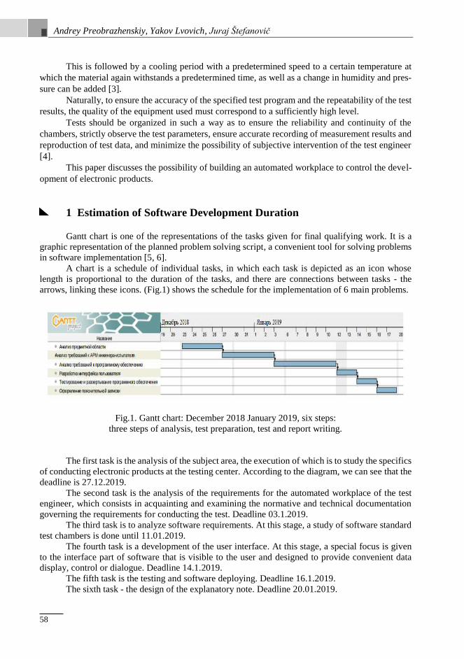
Andrey Preobrazhenskiy, Yakov Lvovich, Juraj Štefanovič
58
This is followed by a cooling period with a predetermined speed to a certain temperature at
which the material again withstands a predetermined time, as well as a change in humidity and pres-
sure can be added [3].
Naturally, to ensure the accuracy of the specified test program and the repeatability of the test
results, the quality of the equipment used must correspond to a sufficiently high level.
Tests should be organized in such a way as to ensure the reliability and continuity of the
chambers, strictly observe the test parameters, ensure accurate recording of measurement results and
reproduction of test data, and minimize the possibility of subjective intervention of the test engineer
[4].
This paper discusses the possibility of building an automated workplace to control the devel-
opment of electronic products.
1 Estimation of Software Development Duration
Gantt chart is one of the representations of the tasks given for final qualifying work. It is a
graphic representation of the planned problem solving script, a convenient tool for solving problems
in software implementation [5, 6].
A chart is a schedule of individual tasks, in which each task is depicted as an icon whose
length is proportional to the duration of the tasks, and there are connections between tasks - the
arrows, linking these icons. (Fig.1) shows the schedule for the implementation of 6 main problems.
Fig.1. Gantt chart: December 2018 January 2019, six steps:
three steps of analysis, test preparation, test and report writing.
The first task is the analysis of the subject area, the execution of which is to study the specifics
of conducting electronic products at the testing center. According to the diagram, we can see that the
deadline is 27.12.2019.
The second task is the analysis of the requirements for the automated workplace of the test
engineer, which consists in acquainting and examining the normative and technical documentation
governing the requirements for conducting the test. Deadline 03.1.2019.
The third task is to analyze software requirements. At this stage, a study of software standard
test chambers is done until 11.01.2019.
The fourth task is a development of the user interface. At this stage, a special focus is given
to the interface part of software that is visible to the user and designed to provide convenient data
display, control or dialogue. Deadline 14.1.2019.
The fifth task is the testing and software deploying. Deadline 16.1.2019.
The sixth task - the design of the explanatory note. Deadline 20.01.2019.

Automated Workplace for the Development of Electronic Components
59
2 Software Testing
The quality of a software product is characterized by a set of its properties that determine it
from the point of interest of concerned parties.
Each of the participants may have a different view of the product, and how high the quality
of the product is. Thus, the formulation of the task of ensuring the quality of a product is translated
into the task of identifying stakeholders, their quality criteria and then finding the optimal solution
that satisfies these criteria.
Testing is one of the most well-established ways to ensure the quality of software
development [13].
The test plan is presented in (Tab.1).
Table 1. Test plan.
Test name
Actions
Expected result
Received
by
result
Launch
applications
User launches the application first time
after installation
A message appears stating
what is necessary to create ad-
min management after
which an eye of registration
admin will appear
Expected results
comply
Launch
applications
User runs the application with an existing
database of users
A window will appear: author-
ization
Expected
results match
User
authorization
User introduces correct login
and password
The main thing will appear in
program window
Expected
results
comply
User
authorization
User enters wrong login or password A message about authorization
error appears
Expected
results
comply
Open list
of users
In the main window:
administrator presses menu
"System" → "List users ... "
A window will open with list of
all registered users
Expected results
comply
To add
user
In the list box of users the administrator
presses "Users" → "Add user ... " and
enters the new user data, and presses save
In the list of users a new
user will appear
Expected results
comply
Edit user In the list of users administrator
clicks right click on user and in
context menu clicks "Edit ..."
A window will appear
for editing user data
Expected results
comply
Delete user In the list box of users the administrator
clicks right click on to the user and
in context menu presses "Delete"
Selected user will be removed
from list
Expected results
comply
Open list
of cameras
In the main window, the administrator
presses the "System menu" → "Camera list
..."
A window will open with
list of all cameras
Expected results
comply
Add camera In the camera list window the
administrator clicks “Cameras” →
"Add the camera ... ",
A window will appear
to add new cameras
Expected results
comply
Edit
the camera
In the camera list window the administra-
tor clicks with the right mouse button on
camera and in the context menu
presses "Change ..."
A window will appear
to edit a camera data
Expected results
comply

Andrey Preobrazhenskiy, Yakov Lvovich, Juraj Štefanovič
60
Table 1. Continued.
Test name
Actions
Expected result
Received
by
result
Remove
camera
In the camera list window administrator clicks right
click on the camera and in context menu presses
"Delete"
Selected camera will
be removed from the
list
Expected
results
comply
Open list of
controlled
parameters
In the camera list window administrator
double clicks on the camera
A window will open
with a list
of controlled camera
parameters
Expected
results
comply
To add
controlled
parameter
In the list box of controlled settings
the administrator clicks "Parameters" → "Add"
A window will open
add controlled parame-
ter
Expected
results
comply
Create
controlled
parameter
In the window to add controlled parameter
user presses a button
A window will open
create new controlled
parameter
Expected
results
comply
Delete
controlled
parameter
In the list box of controlled administrator settings a
right-click on the camera, and in context menu to
press "Delete"
Selected controlled pa-
rameter will be re-
moved from the list
Expected
results
comply
Launch
the test
In main window the user presses item "Tests menu"
→ "Launch test…". In next window then selects the
camera and necessary parameters, then sets duration,
presses run and in next window introduces limits of
control parameters
Window pane launch
tests then task window
limits controlled pa-
rameters
Expected
results
comply
View
progress
trials
In the main window the user double clicks
on selected test item
A window appears
with test progress
Expected
results
comply
3 Description of the Forms of Functional Testing
of the Automated Workplace of a Test Engineer (Fig.2) shows the form “Message about the absence of an administrator in the system”, the
appearance of this form indicates that the administrator account has not yet been created, and you
need to register yourself to start working with the system.
Fig.2. Message about the absence of the administrator in the system.

Automated Workplace for the Development of Electronic Components
61
The user registration form is shown in (Fig.3). To work in the system, you must specify the
type of user, enter your username and password. To complete the registration specify your name and
click "Save".
Fig.3. Admin registration.
The authorization window is shown in (Fig.4). For a successful authorization, you must enter
the login and password specified during registration and click the "Login" button.
Fig.4. User authorization.
After authorization of the user, the main window of the program (Fig.5) opens in which the
user's full name is entered after the “Testing station” field. In the window you can see the full name
of the operator, camera type, test status (“running”, “not running”) and the duration of the test.
Fig.5. The main program window.
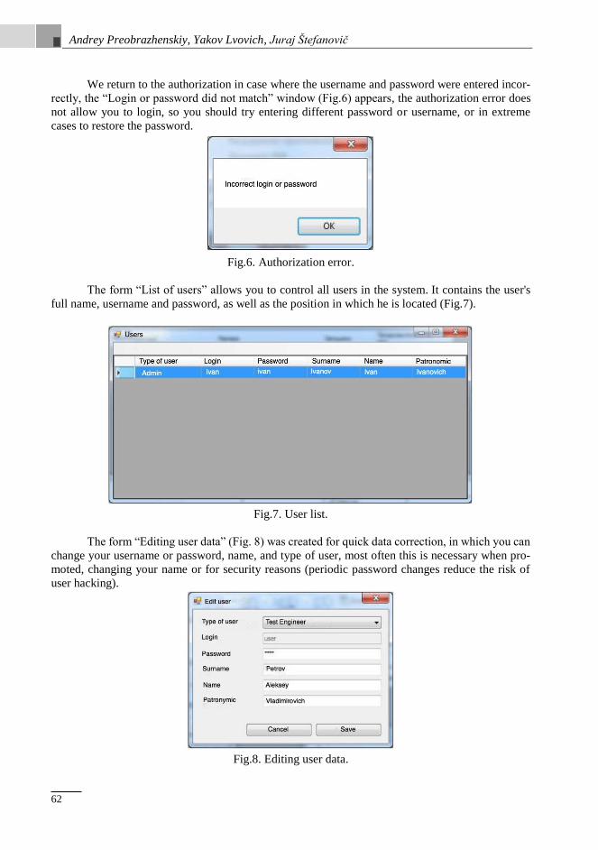
Andrey Preobrazhenskiy, Yakov Lvovich, Juraj Štefanovič
62
We return to the authorization in case where the username and password were entered incor-
rectly, the “Login or password did not match” window (Fig.6) appears, the authorization error does
not allow you to login, so you should try entering different password or username, or in extreme
cases to restore the password.
Fig.6. Authorization error.
The form “List of users” allows you to control all users in the system. It contains the user's
full name, username and password, as well as the position in which he is located (Fig.7).
Fig.7. User list.
The form “Editing user data” (Fig. 8) was created for quick data correction, in which you can
change your username or password, name, and type of user, most often this is necessary when pro-
moted, changing your name or for security reasons (periodic password changes reduce the risk of
user hacking).
Fig.8. Editing user data.

Automated Workplace for the Development of Electronic Components
63
The next window “List of cameras” (Fig.9) allows you to take into account the number of
cameras available in the system.
Fig.9. Camera list.
(Fig.10) shows the “Add camera” form, and to add a new camera, you need to enter the name
of the camera in the “Name” field and click the “Save” button.
Fig.10. Add camera.
To correct the camera name, there is a “Change camera” window; to do this, in the “Name”
field, you must enter the desired camera name, then click the “Save” button (Fig.11).
Fig.11. Change Camera.

Andrey Preobrazhenskiy, Yakov Lvovich, Juraj Štefanovič
64
For each camera there is a separate window with its “Controlled Parameters”, where you can
see and analyze the capabilities of each of the existing cameras (Fig.12).
Fig.12. List of monitored camera parameters.
In the “Add Controlled Parameter” window, you can select already existing parameters and
click the Add button, or add a new parameter (Fig.13).
Fig.13. Add controlled parameter.
After “Creating a new parameter” has been selected, the “New parameter” window appears
where you can specify the name of the parameter and the unit of measurement, then click the “Add”
button, after which the created parameter will be among the monitored ones (Fig.14).
Fig.14. Creating a controlled parameter.

Automated Workplace for the Development of Electronic Components
65
Next, go to the test itself: a “Run test” window was created (Fig.15), where you can select
the desired camera, temperature, voltage or resistance, as well as the duration of the test in minutes.
To start press the “Start” button.
Fig.15. Running the test.
In the “Voltage” window, you can specify the necessary control limits in two fields “min”
and “max” (Fig.16) .
Fig.16. Setting Control Limits.
Fig.17. Test progress.
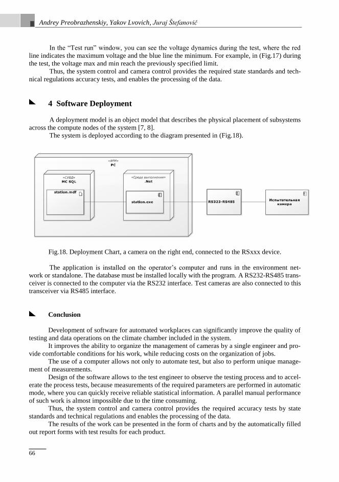
Andrey Preobrazhenskiy, Yakov Lvovich, Juraj Štefanovič
66
In the “Test run” window, you can see the voltage dynamics during the test, where the red
line indicates the maximum voltage and the blue line the minimum. For example, in (Fig.17) during
the test, the voltage max and min reach the previously specified limit.
Thus, the system control and camera control provides the required state standards and tech-
nical regulations accuracy tests, and enables the processing of the data.
4 Software Deployment
A deployment model is an object model that describes the physical placement of subsystems
across the compute nodes of the system [7, 8].
The system is deployed according to the diagram presented in (Fig.18).
Fig.18. Deployment Chart, a camera on the right end, connected to the RSxxx device.
The application is installed on the operator’s computer and runs in the environment net-
work or standalone. The database must be installed locally with the program. A RS232-RS485 trans-
ceiver is connected to the computer via the RS232 interface. Test cameras are also connected to this
transceiver via RS485 interface.
Conclusion
Development of software for automated workplaces can significantly improve the quality of
testing and data operations on the climate chamber included in the system.
It improves the ability to organize the management of cameras by a single engineer and pro-
vide comfortable conditions for his work, while reducing costs on the organization of jobs.
The use of a computer allows not only to automate test, but also to perform unique manage-
ment of measurements.
Design of the software allows to the test engineer to observe the testing process and to accel-
erate the process tests, because measurements of the required parameters are performed in automatic
mode, where you can quickly receive reliable statistical information. A parallel manual performance
of such work is almost impossible due to the time consuming.
Thus, the system control and camera control provides the required accuracy tests by state
standards and technical regulations and enables the processing of the data.
The results of the work can be presented in the form of charts and by the automatically filled
out report forms with test results for each product.

Automated Workplace for the Development of Electronic Components
67
References
[1] Zyablov E.L., Preobrazhensky, Yu. P. (2008) Build an object-semantic model of the control system.
Bulletin of Voronezh Institute of high technologies. No. 3. P. 029-030.
2 Preobrazhensky Yu. P., Zhilin D. V. (2018) Some stages of the history of computer science and
engineering. Bulletin of Voronezh Institute of high technologies. № 3 (26). P. 37-39.
3 Preobrazhensky Yu. P., Tokareva N. M. (2018) Some features of 3d modeling of objects in produc-
tion processes. Bulletin of Voronezh Institute of high technologies. № 4 (27). P. 33-35.
[4] Lvovich I. Ya., Preobrazhensky, Yu.P., Ermolova, V. V. (2014) Foundations of Informatics. Vo-
ronezh, 339 p.
[5] Maximov I. B. (2014) Classification of automated workplaces. Bulletin of Voronezh Institute of
high technologies. No. 12. S. 127-129.
[6] Maksimov I. B. (2014) Principles of formation of workstations. Bulletin of Voronezh Institute of
high technologies. No. 12. P. 130-135.
[7] Preobrazhensky Yu. P., Panevin R. (2010) Yu. Formulation and classification of problems of opti-
mal control of production facilities. Bulletin of Voronezh state technical University. Vol.6. No. 5.
P. 99-102.
[8] Samoilova U. A. (2014) On some characteristics of enterprise management. Bulletin of Voronezh
Institute of high technologies. No. 12. P. 176-179.
Authors
Prof. Andrey Preobrazhenskiy
Doctor of Sciences (Engineering), associate professor,
Voronezh Institute of High Technologies
Prof. Yakov Lvovich
Doctor of Sciences (Engineering), professor,
Voronezh Institute of High Technologies
Ing. Juraj Štefanovič, PhD.
Faculty of Informatics, Pan-European University, Bratislava, Slovakia

Andrey Preobrazhenskiy, Yakov Lvovich, Juraj Štefanovič
68

69
International Journal Volume 8, Number 1, July 2019
Information Technology Applications (ITA)
COMPUTATIONAL MECHANICS
AND OPTIMAL PROGRAMMING PARADIGM
Michal Kráčalík
Abstract:
The aim of the paper is to find an optimal programming paradigm in context of the computational me-
chanics that is mainly focused on the numerical solution of the partial differential equations. Two par-
adigms - procedural and objected oriented (OOP) are compared along with a simple software devel-
opment representing by a GUI. Objected oriented programming can be viewed as a good compromise
among the time required for the production of the code and numerical tests procedures in the compu-
tational mechanics. Procedural programming can be suitable for a quick testing of the numerical solu-
tion of partial differential equation. If the project is extended, the code can be for reusability rebuild to
classes in objected oriented programming. One computational example is shown in the paper and
limitations of the selected programming paradigm are described.
Keywords:
Partial differential equations, objected oriented programming, creep curve, contact.
ACM Computing Classification System:
Applied computing → Physics
Introduction
Computational mechanics is mainly focused on the finding the approximate solution of the
partial differential equations (PDE) [1]. PDEs describe natural laws mathematically and these equa-
tions are usually solved by numerical method like finite element method (FEM), finite difference
method (FDM), boundary element method (BEM) etc. [1]. There is plenty of commercial and open
source specialized “graphical” software like Ansys, Abaqus, Simflow, OpenFOAM, CalculiX and
many more dealing with the numerical solution of PDEs (especially in the field of the continuum
mechanics). Mathematical software like Mathematica, Maple or Matlab are able to handle with
numerical solutions of PDEs as well. Free packages like FEniCS [2] or Code_Aster [3] are in the
development and used in the various field of the continuums mechanics. Software/Toolboxes based
on Matlab have also been developed [4], [5]. Once the solutions of PDE is known, the results are
normally visualized in 2-D or 3-D graphs. Standardly is tested the influence of the input variables
on the results. Therefore, procedural and functional programming are probably the most used in the
computational mechanics. Object-oriented programming (OOP) finds in context of the computa-
tional mechanics mainly place in software development [2], [4].
According to author´s experience, it cannot be predicted whether the piece of “PDE-Testing
code” will serve as a basis for the new software development or not. Hence, choosing the appropri-
ate programming paradigm can be crucial.

Michal Kráčalík
70
The aim of the paper is to compare two programming paradigm and simple software devel-
opment in the framework of Computational mechanics and in prospect of future software develop-
ment. Procedural programming and OOP paradigm will be tested on the computational example;
the simple software development will be expressed through the simple GUI. No exception handling
or unit testing are included in the example and the Python programming language (Ver. 3.7.0) will
be used.
1 Computational Example
The creep curve represents the computational example. The creep curve relates the longitu-
dinal creepage (slip) with the tangential forces in the rolling/sliding contact [6]. Such contact situa-
tion can be found for instance between the rail and the train wheels [7], [8]. The computation is
based on the equations from [6] and the input variables are listed in (Tab.1) (The underlying PDEs
can be found in [9]).
Table 1. The input variables
Variable Unit Notice
Normal force per unit
thickness (𝐹𝑁)
N/mm -
Friction coefficient (𝜇) - 0.5 for steel/steel contact
Young‘s modulus (𝐸) MPa Material constants
Poissons‘s ratio (𝜈) -
Maximum contact
pressure (𝑃𝑚𝑎𝑥)
MPa -
Longitudinal slip (𝛾) - %/100
The full-slip state is defined as:
𝛾fs = 2(1 − 𝜈)𝜇𝑃𝑚𝑎𝑥/𝐺, (1)
where 𝐺 is the shear modulus defined as:
𝐺 = 𝐸/2(1 − 𝜈). (2)
The tangential force 𝑇 is defined as:
𝑇 = {𝜇𝐹𝑁(1 − (1 − |
𝛾
𝛾fs|)2)
𝜇𝐹𝑁
|𝛾| < 𝛾fs
|𝛾| ≥ 𝛾fs (3)
The code was written in the Scientific Python Development Environment Spyder (Ver.
3.3.1) using Python libraries numpy (Ver. 1.15.4) for numerical computation, matplotlib (Ver.
3.0.0) for graph visualisation and tkinter (Ver. 8.6) for GUI. The GUI with the given input variables
is depicted in (Fig.1) and the creepage curve in (Fig.2).
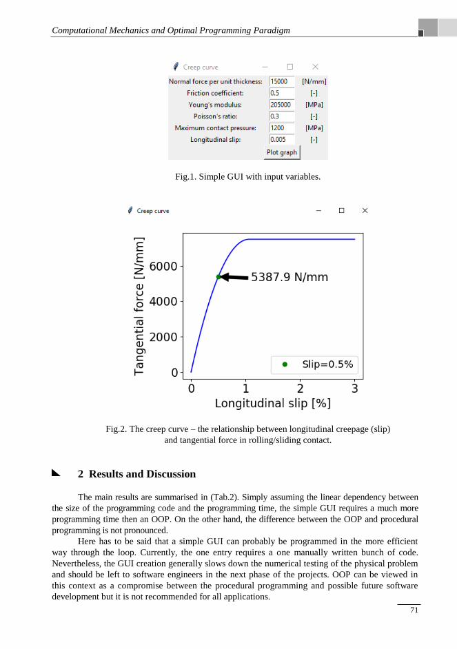
Computational Mechanics and Optimal Programming Paradigm
71
Fig.1. Simple GUI with input variables.
Fig.2. The creep curve – the relationship between longitudinal creepage (slip)
and tangential force in rolling/sliding contact.
2 Results and Discussion
The main results are summarised in (Tab.2). Simply assuming the linear dependency between
the size of the programming code and the programming time, the simple GUI requires a much more
programming time then an OOP. On the other hand, the difference between the OOP and procedural
programming is not pronounced.
Here has to be said that a simple GUI can probably be programmed in the more efficient
way through the loop. Currently, the one entry requires a one manually written bunch of code.
Nevertheless, the GUI creation generally slows down the numerical testing of the physical problem
and should be left to software engineers in the next phase of the projects. OOP can be viewed in
this context as a compromise between the procedural programming and possible future software
development but it is not recommended for all applications.

Michal Kráčalík
72
According to author´s scientific experience, OOP comes on the scene, if the developed pro-
cedure turns into a replicable entity. Otherwise, procedural programming is suitable as well. Once
the piece of code is suitable for an OOP, it is still not time consuming to create a new class. Imple-
menting known physical problem, OOP can be used from the beginning.
Table 2. Assumed linear dependency
between the size of the programming code and time
Paradigm Size of the
programming
code
(in lines)
Programming time
(ratio to Procedural
programming)
Procedural 52 1
OOP 61 1.17
OOP+GUI 157 3.02
The variety of a computational mechanics problem cannot be fully covered by two pro-
gramming paradigm. Recursive programming is used as well [10], [11]. However, recursive pro-
gramming technics can be implemented into the classes in the multi-paradigm language as for in-
stance in the paper used Python.
Conclusion
This paper tests two programming paradigm (procedural and objected oriented) along with a
simple software development at one computational example in order to find an optimal paradigm
suitable for an usage in the computational mechanics. The code written using objected oriented
paradigm needs only a few more line than procedurally written code. The GUI slows a numerical
testing of the underlying partial differential equations and should be left to the software developer
in case of turning the code into a real software development. Procedural programming is suitable
for a quick testing of the ideas without requirements on the reusability of the code. These two pro-
gramming paradigm and functional programming are probably most used in the computational me-
chanics and other programming paradigms are excluded from the paper.
References
[1] Oishi, A., Yagawa, G. (2017). Computational mechanics enhanced by deep learning. Computer
Methods in Applied Mechanics and Engineering, 327, 327-351, ISSN 0045-7825,
doi:https://doi.org/10.1016/j.cma.2017.08.040
2 Rodriguez, M. A., Augustin, C. M., Shadden, S. C. (2019). FEniCS mechanics: A package for
continuum mechanics simulations. SoftwareX, 9, 107-111, ISSN 2352-7110,
doi:https://doi.org/10.1016/j.softx.2018.10.005
3 Antonutti, R., Peyrard, C., Incecik, A., Ingram, D., Johanning, L. (2018). Dynamic mooring simu-
lation with Code_Aster with application to a floating wind turbine. Ocean Engineering, 151, 366-
377, ISSN 0029-8018, doi:https://doi.org/10.1016/j.oceaneng.2017.11.018
[4] Richard, B., Rastiello, G., Giry, C., Riccardi, F., Paredes, R., Zafati, E. Lejouad, C. (2019).
CastLab: an object-oriented finite element toolbox within the Matlab environment for educational
and research purposes in computational solid mechanics. Advances in Engineering Software, 128,
136-151, ISSN 0965-9978, doi:https://doi.org/10.1016/j.advengsoft.2018.08.016
[5] Dallemule, M. (2013). Buckling resistance of arch structures. Ph.D. dissertation,
Slovak University of Technology in Bratislava

Computational Mechanics and Optimal Programming Paradigm
73
[6] Brouzoulis, J. (2014). Wear impact on rolling contact fatigue crack growth in rails. Wear, 314,
13-19, ISSN 0043-1648, doi:https://doi.org/10.1016/j.wear.2013.12.009
[7] Wiedorn, J., Daves, W., Ossberger, U., Ossberger, H., Pletz, M. (2018). Numerical assessment of
materials used in railway crossings by predicting damage initiation – Validation and application.
Wear, 414-415, 136-150, ISSN 0043-1648, doi:https://doi.org/10.1016/j.wear.2018.08.011
[8] Mai, S. H., Gravouil, A., Nguyen-Tajan, M. L., Trollé, B. (2017). Numerical simulation of rolling
contact fatigue crack growth in rails with the rail bending and the frictional contact. Engineering
Fracture Mechanics, 174, 196-206, ISSN 0013-7944
doi:https://doi.org/10.1016/j.engfracmech.2016.12.019
[9] Johnson, K. L. (1985). Contact Mechanics. Cambridge University Press.
doi:10.1017/CBO9781139171731
[10] Sulejmanpasic, T., Ünsal, M. (2018). Aspects of perturbation theory in quantum mechanics: The
BenderWu Mathematica ® package. Computer Physics Communications, 228, 273-289, ISSN:
0010-4655, doi:https://doi.org/10.1016/j.cpc.2017.11.018
[11] Gil, A., Segura, J., Temme, N. M. (2017). Efficient computation of Laguerre polynomials. Com-
puter Physics Communications, 210, 124-131, ISSN 0010-4655
doi:https://doi.org/10.1016/j.cpc.2016.09.002
Author
Dr. Michal Kráčalík
Zurndorf, Austria
[email protected] Dr. Michal Kráčalík (1985) finished his PhD. study at University of Leoben in 2015 and Master study at Faculty of Mechanical Engineering, Slovak University of Technology
(STU) in Bratislava in 2012. He worked as a researcher in Leoben and he currently works as a CAE specialist in the industry. His specialization is investigation of the me-
chanical behaviour of metallic materials using numerical simulations. Dr. Kráčalík is the co-author of several CC articles and he would like to supervise bachelor and master
thesis at universities.

Michal Kráčalík
74

75
International Journal Volume 8, Number 1, July 2019
Information Technology Applications (ITA)
INVESTIGATION OF IMAGE RECONSTRUCTION
ALGORITHM BASED ON THE STRUCTURED
LIGHT METHOD
Igor Lvovich, Oleg Choporov, Eugen Ružický
Abstract:
This paper proposes a new method of recognition of spatial objects on the basis of approaches related
to technical vision. The developed algorithm is used to combine several point clouds by adding a target
object to the scene on the example of a sphere. The algorithm introduces a restriction on some parame-
ters, such as the sphere radius, to reduce the impact of noise in point clouds. Even for point clouds with
overlapping regions, the proposed algorithm is more accurate because the corresponding points are
selected from a continuous and ideal surface, instead of the actual measured points. Furthermore, the
proposed algorithm is less sensitive to target size, point density, noise and the overlap factor, so it is
more accurate than the algorithm of registration of the centers of the spheres and the ICP algorithm.
The proposed algorithm can be used for scanning large, complex, curved surfaces where parts of the
object overlap each other. Experiments and analysis of the proposed algorithm are carried out. To
evaluate the proposed algorithm, three spheres were taken. Two simulations were carried out with over-
lapping data and with non-overlapping data. The size of point clouds is two-thirds of the hemisphere
according to the field of view. Experiments were carried out on the basis of recorded data and real
experimental data, respectively. The simulation was repeated several times with different points of ex-
traction and reproduction of random noise. The statistical results were presented in the table. The prac-
tical significance lies in the possibility of using the results obtained in the study in the field of three-
dimensional scanning.
Keywords:
Image restoration, structured light method, object recognition.
ACM Computing Classification System:
Image and video acquisition, computer vision representations, computer vision problems.
Introduction
Currently, there is a development of methods for processing the characteristics of spatial ob-
jects. Research is carried out in order to create "smart home" systems, robotic systems, remote control
systems, etc. In this regard, relevant research is presented with the development of new approaches
to the recognition of spatial objects based on technical vision.
All image analysis operations are performed using a variety of video sensors, special sources
of structured lighting and modern computing tools equipped with appropriate software. In technical
vision, one of the most important goals is to obtain three-dimensional information from the stage.

Igor Lvovich, Oleg Choporov, Eugen Ružický
76
This problem has been studied for many years. To obtain this information, there are two types
of methods: passive and active. Passive methods extract objects from the scene, such as corners,
edges, lines from images.
Numerous observations of these features allow us to use triangulation methods to recover
three-dimensional information of the scene.
One of the most well-known methods, when two combined cameras are used to obtain this
information, is a stereo vision. However, these methods cannot be used when the scene texture con-
tains few or no functions.
Active methods are used in these situations [1, 2]. Among these systems, structured light is
the most popular. These systems typically consist of a perspective camera and a light emitter, which
can be either a projector or laser projection.
The iterative nearest point algorithm is the main algorithm used in the accurate registration of
three-dimensional point cloud data.
Its accuracy largely depends on the accuracy of the corresponding pairs of points. However,
for some point clouds with constant curvature, such as a plane or a sphere, the method cannot find
the exact matching point pairs and returns an incorrect result.
To solve the above problems, a method of high accuracy registration based on the restrictions
on the spheres based on the method of structured light is proposed.
1 Analysis of the Influence of The Main Factors on Modeling
To evaluate the proposed method, take three spheres and place them as shown in (Fig.1).
Fig.1. Diagram of the relative location of the spheres.
The distances between the spheres are set to 𝐿1 = 36 mm, 𝐿2 = 315 mm and 𝐿3 = 103 mm,
and the radius of the sphere let be r = 25.4 mm. Then the scope of the data modeled in “Matlab” pro-
gram (Fig.2).
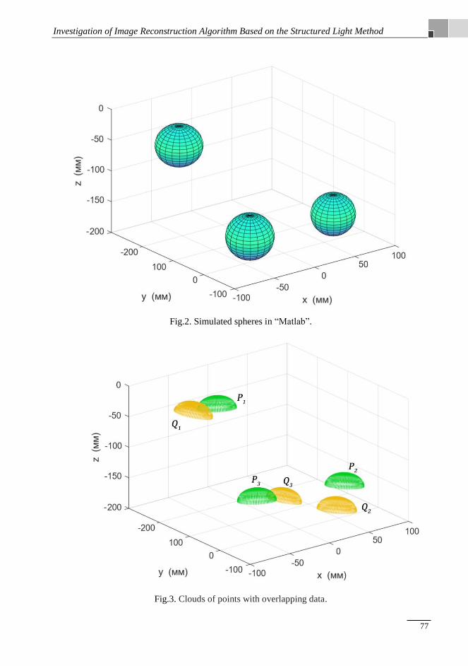
Investigation of Image Reconstruction Algorithm Based on the Structured Light Method
77
Fig.2. Simulated spheres in “Matlab”.
Fig.3. Clouds of points with overlapping data.
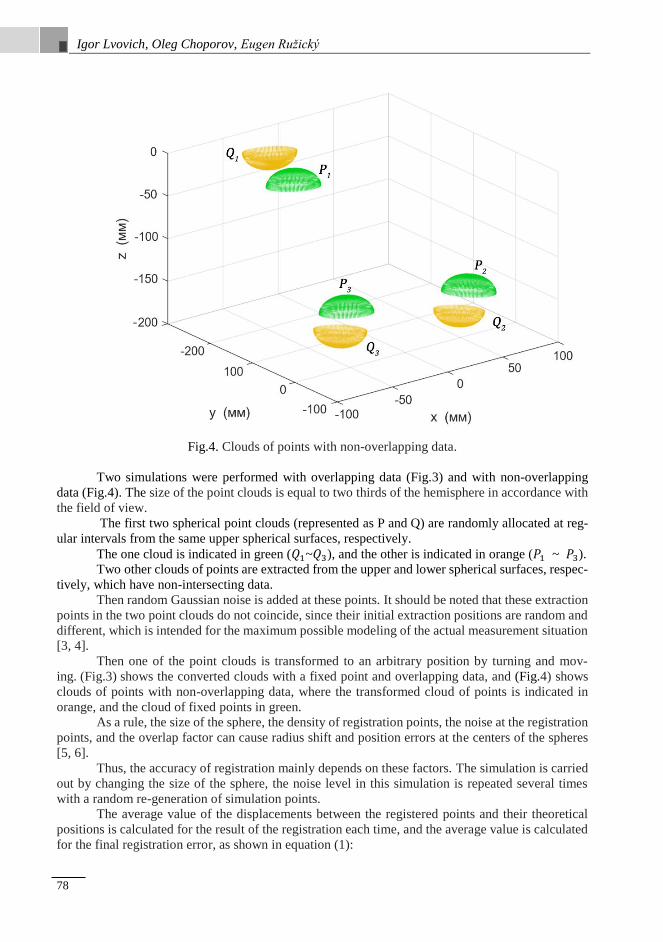
Igor Lvovich, Oleg Choporov, Eugen Ružický
78
Fig.4. Clouds of points with non-overlapping data.
Two simulations were performed with overlapping data (Fig.3) and with non-overlapping
data (Fig.4). The size of the point clouds is equal to two thirds of the hemisphere in accordance with
the field of view.
The first two spherical point clouds (represented as P and Q) are randomly allocated at reg-
ular intervals from the same upper spherical surfaces, respectively.
The one cloud is indicated in green (𝑄1~𝑄3), and the other is indicated in orange (𝑃1 ~ 𝑃3).
Two other clouds of points are extracted from the upper and lower spherical surfaces, respec-
tively, which have non-intersecting data.
Then random Gaussian noise is added at these points. It should be noted that these extraction
points in the two point clouds do not coincide, since their initial extraction positions are random and
different, which is intended for the maximum possible modeling of the actual measurement situation
[3, 4].
Then one of the point clouds is transformed to an arbitrary position by turning and mov-
ing. (Fig.3) shows the converted clouds with a fixed point and overlapping data, and (Fig.4) shows
clouds of points with non-overlapping data, where the transformed cloud of points is indicated in
orange, and the cloud of fixed points in green.
As a rule, the size of the sphere, the density of registration points, the noise at the registration
points, and the overlap factor can cause radius shift and position errors at the centers of the spheres
[5, 6].
Thus, the accuracy of registration mainly depends on these factors. The simulation is carried
out by changing the size of the sphere, the noise level in this simulation is repeated several times
with a random re-generation of simulation points.
The average value of the displacements between the registered points and their theoretical
positions is calculated for the result of the registration each time, and the average value is calculated
for the final registration error, as shown in equation (1):

Investigation of Image Reconstruction Algorithm Based on the Structured Light Method
79
𝑬𝒓𝒓𝑴𝒆𝒂𝒏 =𝟏
𝑵𝒕∙ ∑ [
𝟏
𝑵∑ ||𝒒𝒊́ − (𝑹 ∙ 𝒒𝒊 + 𝑻)||𝑵𝒊=𝟏 ] (1)
where 𝑞𝑖 - vectors representing i-th registered point and its theoretical position, respec-
tively; R and T - solving the rotation matrix and displacement vector, respectively; N - the number
of modeling points, 𝑁𝑡 - simulation time. Then, the final registration errors by equation (1) change
with only one variable while fixing other factors
2 The Influence of the Size of the Sphere
In (Fig.5) are shown the errors caused by changes in the radius of the sphere, where the errors
decrease with increasing radius, since a greater number of points increase the accuracy of positioning
of the centers of the spheres.
Fig.5. Graph of registration errors, on the radius of the sphere.
However, when the radius is greater than 2.5cm, accuracy improves slightly. Accordingly, if
the radius of the sphere is set to r = 25.4 mm it is sufficient for scanning in practice, where the average
error of 3.2 μm is achieved under specified conditions.
(Fig.5) also shows that registration errors with non-overlapping data are similar to results
with overlapping data.

Igor Lvovich, Oleg Choporov, Eugen Ružický
80
3 Influence of Point Density
(Fig.6) shows scanning errors resulting from changes in dot density.
The figure shows that registration errors increase with decreasing point density, and registra-
tion errors with non-overlapping data are also similar to results with overlapping data.
A smaller distance between points can improve the accuracy of registering points, but the
time taken to measure and process data will increase significantly.
Thus, the spacing between the points, being set at about 2 mm × 2 mm, is acceptable under
tuning conditions, where the average error is 3.2 μm.
Fig.6. Graph of registration errors versus change in distance between points.
4 Noise Effect
The effect of noise is divided into two aspects: 1. effect of noise standard deviation and 2. the
effect of the average error:
1. Effect of noise standard deviation.
In (Fig.7) registration errors are shown due to the effect of standard deviation of noise (aver-
age error u = 0).
This shows that errors increase with a growth of the standard deviation of noise, while errors
with and without overlapping data remain unchanged. However, the rate of change is very small.
Even if the standard deviation reaches 150 microns, the error is only about 25 microns. Thus, the
proposed method is not sensitive to standard deviation of noise [7, 8].

Investigation of Image Reconstruction Algorithm Based on the Structured Light Method
81
2. The effect of the average error.
The average error leads to the fact that the radius of the fit has an offset from the previously
known radius. (Fig.8) shows the registration deviations resulting from the influence of the average
error. This shows that registration errors with overlapping data hardly change with an increase in the
average error, but registration errors with non-overlapping data increase significantly with an in-
crease in the average error [9, 10].
Fig.7. Graph of registration errors versus noise deviation.
Fig.8. Registration errors are changed with an average error.

Igor Lvovich, Oleg Choporov, Eugen Ružický
82
The reason is that the shift of the radius leads to the fact that the registered clouds of points
deviate from their theoretical positions. However, for two point clouds with a complete overlap of
their position, the deviations are the same, and this counteracts the registration errors. Thus, the av-
erage error has a great influence on the accuracy of registration, and it must be reduced or eliminated
before registration. The average measurement error is a systematic error and can usually be fixed in
advance.
5 Overlap Effect
(Fig.9) shows errors obtained from the influence of coefficient overlap, wherein the overlap
ratio represents the proportion of regions overlapping with the registered points.
Fig.9. Graph of registration errors versus overlap ratio.
Registration errors do not change significantly (less than 1 micron), regardless overlap. Thus,
the new method is not sensitive to the coefficient of overlap, this method can also solve the problem
of registration with non-overlapping data.
From the above analysis, it is shown that the registration results with non-overlapping data
are consistent with the results with overlapping data, except for the mean error. Therefore, the pro-
posed method is an effective method for registering point clouds with non-overlapping data.
6 The Influence of the Number of Spheres
To check the effect of the number of spheres on the registration accuracy, a curved metal
plate was scanned. A plate with a length of 1 m is measured from several points of view, and
six spheres r = 25.4 mm are located side by side and rigidly fixed with a plate for registration .

Investigation of Image Reconstruction Algorithm Based on the Structured Light Method
83
The plate is a curved sheet, in which it is difficult to obtain data overlap between the concave
and convex surfaces. In addition, concave and convex surfaces have several overlaps, which can
reduce the registration accuracy. Obviously, it is difficult to accurately record clouds of plate points
with existing methods.
The plate is measured in the upper, middle and lower segments, and each segment is measured
from four angles. Thus, about 12 boiling angles must be registered. When using the new top three
spheres are used to register the concave and convex surface of the upper section and register the
upper and middle segments; while the lower three spheres are used to register the lower clouds of
plate points.
To assess the accuracy of the registration of the new method, the measuring point of the
six realms are installed on target areas, and departing radius between the adjustable radius and actual
radius is calculated as shown on the on (Fig.10) where SCR (orange graph) is also used for compar-
ison.
The average radius of displacement is about 0.0380 mm, and the average slope of the SCR is
about 0.1166 mm. This indicates that the registration accuracy of a new method is much better than
SCR.
Fig.10. Graph of dependence of the radius of deviation from the number of spheres.
In general, the new method solves the problems of inaccurate registration with non-overlap-
ping regions or an invariant curvature surface. Theoretically, its accuracy is not limited by the size
of the object being measured, and by adding only some target objects, it is convenient to achieve
high-precision registration.

Igor Lvovich, Oleg Choporov, Eugen Ružický
84
7 Comparison of Registration Accuracy
To verify the accuracy of the SCR, ICP methods and the proposed method, experiments were
carried out on the basis of the recorded data and real experimental data, respectively. The simulation
is repeated several times with different points of extraction and reproduction of random noise. Sta-
tistical results are shown in (Tab.1) and (Tab.2) where registration errors are obtained by equation
(1). Table 1. Registration of results by three registration methods with overlapping data
Method Time (sec)
Registration Error with Overlapping Data
Average
mistake
(µm)
Standard deviation
noise a (µm) Maximum (µm )
SCR 3 10.1 6.7 53.4
ICP 104 22.4 11.1 62.1
New method 96 3.3 1.7 11.6
Table 2. Registration of results by three methods of registration with non-overlapping data
Method Time (sec)
Registration error with non-overlapping data
Average
mistake
(µm)
Standard deviation
noise a (µm) Maximum (µm)
SCR 3 11.4 6.9 60.2
ICP 104 / / 62.1
New method 96 3.2 1.7 11.5
These tables show that the proposed method has the best registration accuracy, the average
error of which is 3.3 μm, and the standard deviation of the noise is 1.7 μm in both cases containing
overlapping data and non-overlapping data; The average SCR error is only about 11.4 microns, and
the standard deviation of the noise is 6.9 microns in these cases; while the average ICP error is 22.4
μm, and the standard deviation of the noise is 11.1 μm for overlapping data, but non-overlapping
data cannot be recorded.
In actual experiments with a measuring system, a standard ball with a radius of 25.4 mm and
a plate of 110 mm × 110 mm with three spherical targets are measured from several types to form
overlapping and non-overlapping data, respectively. The deviation of the surface of the ball from the
reference sphere is less than 5 microns, and the plate roughness does not exceed 5 microns. Only
three spherical targets are used for registration, and the ball and the plate are simply used as the object
of assessment. As registration errors, the residuals of the ball and the plate are used, where the offset
between the radius of the fit and the actual radius value is calculated as the average error for the
ball. The statistical results of registration errors are given in (Tab.3) and (Tab.4).
Registration accuracy is worse than when modeling, which follows from inaccurate experi-
mental data, but still a new method has high accuracy and ICP - the worst, which is similar to the
simulation results. As a rule, the ICP algorithm is a high-precision registration method, but the cor-
responding pairs of points from the two extracted clouds of points are not sufficiently accurate, which
leads to an incorrect result. The noise causes errors in fitting the centers of the spheres, which leads
to inaccurate alignment of the two cloud points using the SCR method.

Investigation of Image Reconstruction Algorithm Based on the Structured Light Method
85
Table 3. Registration of results by three registration methods with overlapping data
An object Method
Registration error with non-overlapping data
Average
mistake
(mm)
Standard deviation
noise a (mm) Maximum (mm)
Ball
SCR 0.036 0.028 0.144
ICP 0,260 0.130 0.433
New method 0.012 0.023 0.107
Plate
SCR 0 0.041 0.121
ICP 0 0.104 0,224
New method 0 0.020 0.069
Table 4. Registration of Results with Non- Overlapping Registration Methods
An object Method
Registration error with non-overlapping data
Average
mistake
(mm)
Standard deviation
noise a (mm) Maximum (mm)
Ball
SCR 0.048 0.033 0.112
ICP / / /
New method 0,009 0.028 0.119
The new method additionally optimizes the transformation matrices with a limited radius after
obtaining a good initial value using the SCR method. Therefore, we obtain more accurate
corresponding pairs of points, instead of an extracted cloud of points, which is a key factor in
obtaining an optimal convergence result. Therefore, the proposed method achieves the best accuracy.
Conclusion
In this paper we propose a new method for registering constraints using spheres, which is
adapted for precision registration multipoint cloud points with non-overlapping regions.
The proposed method introduces the use of the restriction of some parameters to reduce the
effect of noise in point clouds. Even for point clouds with overlapping areas, the proposed method is
more accurate, since the corresponding points are selected from a continuous and ideal surface, in-
stead of real discrete measured points. Conversion parameters are determined by the optimization
method with weight functions. In this case, the effect of large noise is reduced, and the registration
stability is improved. Modeling and experimental results show that the proposed method effectively
solves the problems of impossible registration or registration with low accuracy. In addition, the
proposed method is less sensitive to the size of the target, the density of points, noise, and the overlap
coefficient; therefore, it is more accurate than the method for registering the centers of the spheres of
the center and the general ICP algorithm. Theoretically, not only spheres, but also other objects, such
as cones, cylinders, can be used as target objects during registration. Therefore, the proposed method
is more accurate than the method of registering the centers of the spheres and the general ICP algo-
rithm.
The proposed method can be used when scanning complex, curved surfaces.

Igor Lvovich, Oleg Choporov, Eugen Ružický
86
References
[1] Preobrazhensky A. P. (2003) Prediction of radar characteristics of objects with radioabsorbing coat-
ings in the wavelength range. Telecommunications. 2003. No. 4. P. 21-24.
2 Preobrazhensky A. P. (2004) Prediction of radar characteristics of objects in the wavelength range
using the results of measurements of scattering characteristics at discrete frequencies. Telecommu-
nications. No. 5. P. 32-35.
3 Preobrazhensky A. P., Choporov O. N. (2004) Method of forecasting radar characteristics of objects
in the wavelength range using the results of measurements of scattering characteristics at discrete
frequencies. Management systems and information technologies. № 2 (14). P. 98-101.
[4] Preobrazhensky A. P., Choporov O. N. (2004) Algorithms for predicting radar characteristics of
objects in the restoration of radar images. Management systems and information technologies. №
5 (17). P. 85-87.
[5] Preobrazhensky A. P. (2003) Investigation of the possibility of determining the shape of an object
in the vicinity of the restoration of local reflectors on the surface of objects by their backscattering
diagrams. Telecommunications. No. 4. P. 29-32.
[6] Preobrazhensky A. P., Hukhryansky Yu. P. (2005) Construction of radar images of objects. Bulletin
of Voronezh state technical University. Vol.1. No. 8. P. 20-23.
[7] Shutov G. V. (2014) an Approximate model to estimate the average characteristics of the scattering.
Modern science-intensive technologies. No. 5-2. P. 60.
[8] Baranov A.V. (2013) Some features of ray methods for calculation of electromagnetic wave prop-
agation characteristics. Bulletin of Voronezh Institute of high technologies. No. 10. P. 9-13.
[9] Morgunov V. S. (2014) Modern methods of calculating the propagation of radio signals in the prem-
ises. Bulletin of Voronezh Institute of high technologies. No. 12. P. 136-139.
[10] Komaristaya K. O. (2019) issues relating to the processing of noisy and distorted images. Bulletin
of Voronezh Institute of high technologies. № 1(28). P. 33-35.
Authors
Prof. Igor Lvovich
Doctor of Sciences (Engineering), professor
Voronezh Institute of High Technologies
E-mail: [email protected]
Prof. Oleg Choporov
Doctor of Sciences (Engineering), professor
Voronezh state technical university
Assoc. Prof. Eugen Ružický, PhD.
Faculty of Informatics, Pan-European University, Bratislava, Slovakia
Main interests are: system analysis, enterprise computing.

87
International Journal Volume 8, Number 1, July 2019
Information Technology Applications (ITA)
DEVELOPMENT OF AN APPLICATION
FOR THE E-STORE ON ANDROID
Andrey Preobrazhenskiy, Emma Lvovich, Kseniya Lvovich
Abstract:
This paper discusses the possibility of creating an application for customers of the online store based
on the Android operating system. Android is a platform that allows the developer to abstract from the
kernel and write in high-level languages. The framework offers a large API that allows you to create
programs of completely different profiles. Android architecture is formed from many components. Each
higher-level component is based on lower-level elements. The application is developed by client-server
architecture. The client is the program itself. The server is a CMS platform on which the website of the
online store is deployed. The latter provides a public API for the organization of external interaction
with the site. Communication between the client and the server is provided by http requests and JSON
messages. The basic functional requirements for the application are described. The scenario of regis-
tration in the form of a flowchart is illustrated. The scenario of interaction with the catalog is given.
Shown, Kaim realized scenario of the order. Testing was carried out on the emulator and on the Sony
Xperia M2 device. It shows how the user works with products.
Keywords:
Сomputer application, online store, Android, user.
ACM Computing Classification System:
Distributed systems organizing principles, software functional properties,
specialized application languages.
Introduction
Today Android is the most popular operating system for smartphones. According to the re-
search Gartner, now Android OS is used more, than in 87% of mobile devices. Of course, its such
prevalence involves a large number of developers. Certainly, today Android is the most demanded
system for mobile devices. Moreover, there is an opportunity to develop applications for this platform
and to sell them in special online store. A set of development tools (Android SDK) is available for
free to everyone [1].
With the growing demand for various applications for mobile platforms, the sales of relevant
programs are also growing. Today, an increasing number of companies are striving to have their own
smartphone application, so that the service catalog can always remain with the client “at hand”.
However, Android is not the only one operating system in the market. Consequently, there
may be problems with the compatibility of applications on different operating systems, as each sys-
tem developer tries to make it different from the others and more convenient for the ultimate user.
In the IT industry there is an expectation to rapidly increase the volume of software for mobile
devices.
So, today the development, introduction and support of mobile programs for the Android op-
erating system is a relevant direction in the IT sphere.

Andrey Preobrazhenskiy, Emma Lvovich, Kseniya Lvovich
88
The share of the Android-applications is growing: they allow users to optimize the time to
search for products, quickly find the necessary information in the network, some of them even offer
some functions with voice control.
1 Architectural Features
Android is a platform that allows developers to abstract from the core and write in high-level
languages. The framework offers a big API that allows to create programs of a completely different
profile. Android architecture is made up of many components. Each component of a higher level is
based on elements of a lower level. (Fig.1) illustrates the main components of Android.
Fig.1. Main components of Android.
The basis of the platform is a modified Linux-kernel. Also at this level there are drivers for
input/output devices. The core is a base of the whole operating system. Besides, the core is respon-
sible for management of memory, processes, network support and etc.
2 Architecture of the Application
The application is developed on the client-server architecture. The client itself is the program.
The server is the CMS platform on which will unroll the website’s online store. The last one provides
public API for the organization of external interaction with the website. Communication between the
client and the server is provided using http requests and JSON messages.
Operation of the Web server is not considered, because work with it is managed through the
applied interface, and is perceived as a "black box"
The application has the following entities activity: LoginActivity, RegistrationActivity, Men-
uActivity, CatalogActivity, ProductActivity, BasketActivity, OrderActivity, PaymentActivity and
CabinetActivity.

Development of an Application for the E-store on Android
89
LoginActivity represents the window displaying a greeting and a form of input of registration
data with two fields: e-mail or phone and password. The form is supplied with the login button and
also password recovery and registration buttons. After confirmation of the entered data and verifica-
tion of their correctness by the system, the user opens an activity that displays a catalog [2].
From the system, in addition to displaying the dialog box to the user, a request is formed in
the server to verify the authenticity of the entered data and, based on the CMS response, the decision
to authorize the user. If registration data are correct, the system redirects it to the directory.
RegistrationActivity provides an opportunity for a new client to register on the site. The win-
dow has a welcome text, an invitation to register and a standard form: an e-mail input field and also
two fields for input of the password - the second to eliminate the input error in the first one. Under
the form there is a button to confirm registration. After registration confirmation the user is redirected
to a personal account.
In turn, the system checks at once the matches of the entered passwords and, if they match a
server request is created for signing up the new user in to the database. In case of success the system
reports to the client about completion of process and redirects it to a personal account [3].
From the application side, a request is made to the CMS in order to get a list of goods and
their properties, processing the response JSON message and passing the parameters to activity for
displaying them to the client.
ProductActivity gives the customer the opportunity to view the full properties of the product
and additional photos if they’re available. The user gets to this window by clicking on any product
in the catalog. Here, photos are available to the client in an enlarged size; if they are several, then
browsing is organized; as well as in the table view, with the extended characteristics at a separate
position for product description [4].
The system in this case provides the provision of this information to the program user by
contacting the server to obtain it, processing the received data and providing them in a convenient
form for the client.
BasketActivity provides the functionality of a classic basket. In this window, the client is
available to view all the products that he decided to order. Here you can see the names of the catalog
items, the number of units ordered, the amount separately for each item and the total value of all
products. The activity is supplied with the button "issue the order" after which pressing the user gets
to an order window. There is an opportunity to increase or decrease the number of items ordered.
The system adds to the cart the products from catalog, while there is no access to the server.
The application has a position in a table form, convenient for viewing. The program adds or deletes
a position in the basket.
OrderActivity allows to issue user's order. In this window, the user displays the number of
items ordered and the amount of the order. The customer here has the opportunity to enter their
contact details: phone, email, card details and choose the desirable payment method: as an individual
or as a legal [5].
The application in this case checks the correctness of the entered data, then informs the user
that his order has been successfully issued, that product data are valid, or specifies the reason for
which next continuation is impossible for client editing. Then the application redirects the user to the
order payment window.
PaymentActivity is called to pay for the order by the user. It is proposed to pay by bank trans-
fer as an individual or as a legal entity based on the choice of the client in the checkout window. For
individuals, there is a form for entering bank card details. For legal entities - bank details of the
organization for invoicing by the name of the company-buyer. After the indication of all data of the
user of the application, the client is redirected to the payment system window to confirm the payment,
in case the user pays the order as an individual, or the client is informed about the successful execu-
tion of the order with a request to expect the manager's call for confirmation and the account for
payment [6].

Andrey Preobrazhenskiy, Emma Lvovich, Kseniya Lvovich
90
The application opens a payment system window for the user with a one-time security code
entry form. After authorization of payment, the system returns the client to the order window, where
he is informed about the successful completion of payment. After the system writes the order infor-
mation [7] to the database using a request to the server.
CabinetActivity provides the user with the functionality to manage information about them-
selves. There, the client has the opportunity to leave personal information, such as name, phone num-
ber and email.
3 The Functionality of the Program
The system must be an application running on the Android operating system. The program
should have the functionality to view the product catalog, design and order products, as well as have
a personal user account and the ability to register a new client.
Functional requirements, General:
1. The system should allow to register a user
2. The system should allow editing information about users
3. The system should show a catalog of products
4. The system should display the detailed properties of each product
5. The system should provide the ability to create an order and pay for it
Registration Functionality:
The user enters the registration window. Here he enters his credentials: email, password. Af-
ter the client confirms the correctness of the entered data and presses the "Register" button.
In turn the system checks correctness of input of mail, phone and also coincidence of pass-
words. After that, a request is made to the server, and the encrypted data is sent to the server, where
register in the database. (Fig.2) illustrates the registration script as a flowchart.
Fig.2. Registration script.

Development of an Application for the E-store on Android
91
Catalog functionality:
To get to the catalog, the user needs to select the appropriate item in the menu. At the same
time, he gets into a new window, where he can view the currently available products in the form of
tiles. When you click on the tile product, the user opens a new window with detailed characteristics
and photos. To return to the catalog window, we need to press the button "back".
When a user goes to the catalog, the system forms a request to the server to get a list of
products and their properties. The application displays a list on the screen. (Fig.3) shows the user
scenario in the directory.
Fig.3. The scenario of interaction with the catalog.
Functional order:
The user enters the order menu by clicking on the "basket" button. It displays the name and
number of products selected by the customer for the order. A transition to the order completion menu
is made by the button "issue an order". Here, the application user enters his contact information for
contacting and confirming the order, as well as the delivery address. After confirmation by the client,
the system opens a window with a payment form. In it, the user enters data for payment of the order
and confirms them.
Upon confirmation of the order by the client, the system authorizes the payment and makes a
request to the server to save the order in the database. Next, the system sends an e-mail to the man-
ager's mail. (Fig.4) illustrates the order scenario.
Testing the application:
Testing was performed on the emulator and on the Sony Xperia M2 device. The following
errors were identified and corrected with the help of testing:
1. Font clipping;
2. Indents that do not match the design;
3. Errors with the display of the cursor;

Andrey Preobrazhenskiy, Emma Lvovich, Kseniya Lvovich
92
4. Invalid field sizes;
5. Incorrect display of messages for the user;
6. Incorrect display on devices with a large screen size.
Fig.4. The order scenario.
4 Implementation of the Software
The main activity of the application is the entrance activity. Starting the application, the user
gets to an entrance window where he is offered to enter the login and the password. Also there is a
registration button. In the (Fig.5) entrance activity is presented.
The activity receives the login password entered and transfers them to the input of the Res-
tAssured library.
It allows you to create JSON objects from various Java data structures, and also simplifies
working with the REST API. Using the specified library, the application sends a request to the server
to authorize the user. It is also possible to work with the response from the server using RestAssured.
It will make analysis of the response message and will transfer to activity the answer from the server
with confirmation or denial of authorization.
(Fig.6) shows a window with a catalog of products. The latter are arranged with tiles, showing
a miniature photo, the name of the product and its price. By clicking on the photo, the application
will go to the window with advanced product features and additional photos.
If the client wants to see the detailed properties of a particular product, he can click on the
tile of the desired product. After that, he gets into the product card, where he will be able to view
additional information about the product. (Fig.7), (Fig.8) and (Fig.9) show the item card.

Development of an Application for the E-store on Android
93
Fig.5. Application entrance activity: Welcome, Email, Password, Enter, Registration.
Fig.6. Product catalog window: material description and price.

Andrey Preobrazhenskiy, Emma Lvovich, Kseniya Lvovich
94
Fig.7. Enlarged product photo: a sponge glass gravel, diameter and volume.
Fig.8. Availability and item of products: soil drainage product, price, quantity, into basket.

Development of an Application for the E-store on Android
95
Fig.9. Detailed product description: a sponge glass gravel, size, application field, package.
Fig.10. Navigation menu of the application:
Cultivation products - Catalogue, Basket, Personal, Enter.

Andrey Preobrazhenskiy, Emma Lvovich, Kseniya Lvovich
96
Fig.11. Basket: product name, volume, price, amount (1), total, confirm.
(Fig.10) presents the application menu. The menu has navigation buttons that allow the user
to go from one window to another. The client has the opportunity to go from here to the catalog, to
the personal account or to the basket.
After clicking of the “Basket” button the client will be able to see products which he wishes
to buy, also their quantity and the amount. (Fig.11) shows the interface of a basket.
Conclusion
The analysis showed that the development and implementation of a mobile application will
contribute to the promotion of the product and increase the company's profit, because potential cus-
tomers will be able to study the catalog using a smartphone. Today, commercial Internet projects are
a huge success, respectively, a company that has its own high-quality website on the network has an
advantage over its competitors. Especially if the organization has developed a mobile application
that is integrated with the site.
A smartphone application is more a fashion tool; it is necessary that it left a positive impres-
sion of the use of customers. The convenience and speed of access to information plays a large role
today, therefore, existence of the mobile application stimulates sales and attracts potential clients.
Therefore high-quality development mobile ON - one of paramount tasks for the large organization.
Mobile application for online store will definitely attract customers, especially the category of people
with high employment. Now, it will take significantly less time to purchase the required amount of
substrate, especially since it is not necessary to buy the foam glass substrate live: its appearance and
fraction will be the same from batch to batch, you do not need to come to the office to see it with
your own eyes. Separately, it is worth mentioning the category of people who, in principle, are more
convenient to visit stores online.

Development of an Application for the E-store on Android
97
Also, many people are somehow connected with the global network and it will probably be
easier for them to visit an order in a virtual stores. Moreover, there the consumer can view a full
range of goods quickly and get any information about the selected product.
A modern smartphone or tablet can completely replace all the functions of home computers.
One of the most advanced operating systems for mobile devices is Android. Please note that mobile
devices work on applications specifically written for their use, as well as applications implemented
in a web form.
As a result of the work described above a goal was achieved: the application for the client of
the “IdealGrunt online store” is developed. Objectives were also carried out. In the course of work
selected architectural features of the Android platform were studied and used.
Testing process allowed to reveal some defects of application and to correct them in the
course of development.
References
[1] Vinokurov A.V. (2019) Features of the use of reactivex technology in mobile applications for the
Android operating system. Bulletin of Voronezh Institute of high technologies. № 1(28). P. 53-57.
2 Preobrazhensky Yu. P. (2018) Information technologies used in the field of management. Bulletin
of Voronezh Institute of high technologies. № 2(25). P. 43-46.
3 Kostrova V. N., Gusev A.V. (2018) Methods and tools for developing and evaluating the quality of
web applications. Bulletin of Voronezh Institute of high technologies. № 2(25). P. 75-78.
[4] Kamakin V. D., Lvovich I. Ya. (2018) Problems of protection of electronic documents. Bulletin of
Voronezh Institute of high technologies. № 4(27). P. 64-66.
[5] Melnikova T. V. (2016) Some features of business analyst's work in it-sphere. Modeling, optimiza-
tion and information technologies. № 1 (12). P.5.
[6] Chernikov S. Yu., Korolkov R. V. (2014) the Use of system analysis in the management of organ-
izations. Modeling, optimization and information technologies. № 2 (5). P. 16.
[7] Samoilova U. A. (2014) On some characteristics of enterprise management. Bulletin of Voronezh
Institute of high technologies. No. 12. P. 176-179.
Authors
Prof. Andrey Preobrazhenskiy
Doctor of Sciences (Engineering), associate professor
Voronezh Institute of High Technologies
Ass. prof. Emma Lvovich, PhD.
Candidate of Sciences, associate professor
Voronezh Institute of High Technologies
Kseniya Lvovich
postgraduate student
Voronezh Institute of High Technologies

Andrey Preobrazhenskiy, Emma Lvovich, Kseniya Lvovich
98

99
International Journal Volume 8, Number 1, July 2019
Information Technology Applications (ITA)
IMPLEMENTATION AND TESTING OF TEXT
RECOGNITION ALGORITHM ON MOBILE DEVICES
Oleg Choporov, Igor Lvovich, Juraj Štefanovič
Abstract:
A large number of people every day are faced with a situation where they need to transfer the text from
the image or various documents to digital format. This is a routine work that requires a lot of time, care
and effort. In most cases, a mobile phone, unlike a scanner, is always there. The mobile application will
allow you to quickly transfer the necessary documents to the digital version, and the format of the cre-
ated document, DOC will allow you to immediately start working with it, without losing additional time
to convert the file to an available format for editing. The aim of the work is to develop a mobile appli-
cation for text recognition from a graphic image for Android devices. This program is implemented in
object-oriented programming language Java, using the development environment Android Studio. The
analysis was done of the existing API and existing methods of text recognition. The most suitable meth-
ods were selected and integrated into the application.An algorithm for creating and storing a file in the
memory of a mobile device was developed and implemented, as well as an algorithm that will allow you
to get the files created by the application from your mobile phone. The ability to send files is implemented
too. An application interface was developed and implemented. The application was tested.
Keywords:
Image recognition, program, application.
ACM Computing Classification System:
Distributed systems organizing principles, software functional properties,
specialized application languages
Introduction
The development of a mobile application based on the Android OS, for text recognition from
a graphic image is an actual topic. This is due to the fact that a large number of people daily face a
situation where they need to transfer text from an image or various documents to a digital format [1].
This is a routine work that requires a lot of time, care and effort. In most cases, a mobile
phone, unlike a scanner, is always there.
The mobile application will allow you to quickly transfer the necessary documents to the
digital version, and the format of the created document, DOC, will allow you to immediately start
working with it, without losing any additional time to convert the file into an accessible format for
editing.
The DOC document format is a feature of this application, since almost all analogues allow
you to save files in PDF format, which is not convenient, since this format is not suitable for editing.
The goal is to develop a mobile application for text recognition from a graphic image for
Android devices.

Oleg Choporov, Igor Lvovich, Juraj Štefanovič
100
To implement the application, the following tasks were set:
1. Analyze and disassemble existing text recognition methods.
2. Analyze and parse existing APIs. Choose the most suitable and integrate it into the appli-
cation.
3. Develop and implement an algorithm for creating and storing a file in the memory of a
mobile device.
4. Develop and implement an algorithm that allows you to receive files created by the appli-
cation from a mobile phone and realize the possibility of sending them.
5. Develop and implement an application interface.
1 Installing the Application
In order to use the application, you must first install it. The installation file permits APK, it
is standard for all versions of the Android operating system [2]. The name of the installer Docu-
ment_reader_1.0, an example in (Fig.1). The application icon is currently standard. It is presented in
the form of a square image with the logo of the Android OS.
To start the installation, you must click on the icon of this application. The system will auto-
matically start the installation process and a window will open before the user informing you that
this application does not require special permissions and asking: Do you really want to install it?
An example of this item is in (Fig.2). If the user clicks the "Cancel" button, the installer will
close and the application will not be installed. If, at this stage, click the "Install" button, the installa-
tion program will automatically redirect the user to the next page of the installer.
Fig.1. Installer file.
The second page of the installer displays the installation progress itself. The system unpacks
files and registers them in the telephone system for further use.
The installation step is displayed as a green bar in the center of the screen, which symbolizes
the remaining and elapsed time, an example in (Fig.3).
To complete the installation, the user simply needs to wait until the bar is completely full.
The waiting time is always individual, depending on the processor that is installed in the
mobile device, the amount of RAM and the write speed of the internal or external drive, depending
on which one is being installed.
Most often, the installation takes about 2-3 minutes, in some cases, the time may be longer,
due to the reasons described earlier.

Implementation and Testing of Text Recognition Algorithm on Mobile Devices
101
Fig.2. Installation Initial Page: information, button cancel and install.
Fig.3. Installation Process.
After the installation process is completed, if the user has the built-in antivirus installed, the
system will start checking the installed files, an example is shown in (Fig.4). This test also takes
some time and depends on the same conditions as the installation. It allows you to protect the user's
device from malicious programs, confirms that the installation was performed correctly and the ap-
plication will work correctly.

Oleg Choporov, Igor Lvovich, Juraj Štefanovič
102
If the user does not want to wait, he can click the "Cancel" button, the check will stop, but
the application will be installed. This action poses a security risk and is not recommended. If the user
just waits, the system upon completion of the check will display a new page that informs him about
the successful check, an example is shown in (Fig.4). On this page, you must click the "Finish" button
and proceed to the operation of a successfully installed and verified program.
Fig.4. The beginning and the end of the test.
2 Application Operation
After the application is installed, a shortcut will appear on the desktop or menu (depending
on the Android OS version). It is a green square with the company logo of the Android operating
system. The names of this label "Document reader". The example is in (Fig.5). To start the applica-
tion, you need to click once on the icon of this application.
After starting, the user sees the main menu and application interface, an example is (Fig.6).
When you click on the “Take a photo” button, the system will ask the device for permission to use
the camera, an example is (Fig.7).
If you click the "Reject" button, the application will not get access to the camera and further
work with it will not be possible. You must select "Allow". When obtaining rights, the program must
be restarted. This procedure is performed once during the initial launch of the application. After all
these actions, the standard Camera application is launched, which is installed in every smartphone
that can take photos. The user needs to focus the camera lens on the text that he wants to scan. The
image of the text should be in focus and readable. The phone must be kept in a horizontal position,
since the text reading algorithm works in such a way that correct text recognition will occur only
when all these conditions are met. To take a picture you need to click on the button responsible for
creating the image. Depending on the application, it may have its own unique look. The application
will save the captured image in the memory of your device for future use.

Implementation and Testing of Text Recognition Algorithm on Mobile Devices
103
It can be found by following the Android / data / com / example.skript.documentreader / files
/ Pictures path on the mobile device itself. With these images you can work, as with any photos on
the device. After the snapshot is taken, the next page of the application opens, where its main actions
take place, an example is (Fig.8).
Fig.5. Application Label: Document.
Fig.6. Main Menu.

Oleg Choporov, Igor Lvovich, Juraj Štefanovič
104
Fig.7. Camera access: allowing to the application to use camera?
Fig.8. Document Creation Page.
In the upper part are displayed all the images that will be recognized and included in the
created document. Each selected file is a new document page.
When you click on the "Take another photo" button, the system will reopen the "Camera"
application to create another image. All actions on the requirements for photographs have been de-
scribed in the manual earlier. They remain unchanged for this situation. The photo taken is also stored
in the phone's memory and is added to the top of the form to the other, existing files.
Clicking on the "Take from gallery" button will open the standard "Gallery" application with
the latest saved images in the phone's memory, which you can select by tapping on the necessary.
The graphic file will be added to the list and displayed at the top of the previous menu, where the
first photo taken will be displayed.
The field is displayed in the center of the page, it is necessary to enter the text in it, example
(Fig.9). This will be the name of the file that will create the application. You can enter letters, symbols
and numbers in this field. To create a file, click on the "Create file" button. The created file will be
in the DOC format and located in the phone's memory on the Android / data / com / exam-
ple.skrpt.documentreader / files / documents path.

Implementation and Testing of Text Recognition Algorithm on Mobile Devices
105
Fig.9. The input field for entering the file name.
Clicking the “Check documents” button opens a list of files that were created by the applica-
tion or added by the user to the “Documents” folder on their own, for example, (Fig.10). These files,
the user can edit, send or move on his request.
Fig.10. List of Documents.
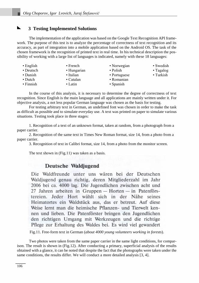
Oleg Choporov, Igor Lvovich, Juraj Štefanovič
106
3 Testing Implemented Solutions
The implementation of the application was based on the Google Text Recognition API frame-
work. The purpose of this test is to analyze the percentage of correctness of text recognition and its
accuracy, as part of integration into a mobile application based on the Android OS. The task of the
chosen framework is the recognition of printed text in real time. In his technical description the pos-
sibility of working with a large list of languages is indicated, namely with these 18 languages:
• English
• Deutsch
• Danish
• Dutch
• Finnish
• French
• Hungarian
• Italian
• Catalan
• Latin
• Norwegian
• Polish
• Portuguese
• Romanian
• Spanish
• Swedish
• Tagalog
• Turkish
In the course of this analysis, it is necessary to determine the degree of correctness of text
recognition. Since English is the main language and all applications are mainly written under it. For
objective analysis, a not less popular German language was chosen as the basis for testing.
For testing arbitrary text in German, an undefined font was chosen in order to make the task
as difficult as possible and to simulate everyday use. A text was printed on paper to simulate various
situations. Testing took place in three stages:
1. Recognition of a text of an unknown format, taken at random, from a photograph from a
paper carrier.
2. Recognition of the same text in Times New Roman format, size 14, from a photo from a
paper carrier.
3. Recognition of text in Calibri format, size 14, from a photo from the monitor screen.
The text shown in (Fig.11) was taken as a basis.
Fig.11. Free-form text in German (about 4000 young volunteers working in forests).
Two photos were taken from the same paper carrier in the same light conditions, for compar-
ison. The result is shown in (Fig.12). After conducting a primary, superficial analysis of the results
obtained with a glance, it can be noted that despite the fact that the photographs were taken under the
same conditions, the results differ. We will conduct a more detailed analysis [3, 4].

Implementation and Testing of Text Recognition Algorithm on Mobile Devices
107
Recognizable text contains 569 characters, 88 words. Judging by the first example, the appli-
cation was able to recognize the text correctly, but for some reason the characters “a”, “s”, “s”, “h”
were added, only 4, which were not in the original version. In the example, they are underlined in
red. Despite this, the result was pretty good. With a more accurate calculation, it becomes clear that
the error of 4 characters from 569 was only 0.7%. Therefore, the text is correctly recognized at 99.3%.
After retesting, using the same text, a more positive result is seen. The application was able
to recognize the text completely correctly, without any errors. A positive result was 100%. Improve-
ment is achieved by training the neural network; after the first attempt, the system makes it easier to
recognize almost identical images.
The second step is to test the recognition of the same text, given in the Times New Roman
format, size 14, from a photograph from a paper medium. The example we can see in (Fig.13).
At the first result obtained, a similar picture is displayed, which was in the first stage. When
recognizing the text from the first photo, it is clear that the application was mistaken several times,
namely the word “Jahren” was recognized as “ahren” and the word “seines” was recognized as
“senes”. The system made 2 errors out of 569 characters. Having calculated the percentage ratio, it
becomes clear that the error in the result obtained is 0.35%. Therefore, the text is correctly recognized
at 99.65%. This result is better than at the previous stage.
After retesting the second stage, using the same text, a positive result is seen. The application,
like last time, on the second attempt was able to recognize the text completely correctly, without any
errors. A positive result was 100%. This is due to the fact that the neural network is trained and the
recognition becomes more accurate.
The third stage of testing is the recognition of text in Calibri format, size 14, from a photo
from the monitor screen. The photo was taken in good quality and with sufficient illumination, but
at the same time the camera focuses well on the pixels of the screen itself. In addition, the monitor
from which the photo was taken is curved. All these facts distort the resulting image, which creates
additional difficulties for the system in recognizing text, an example is (Fig.14). Even in such a com-
plex task, the system performed well. Despite the experience of the previous steps, this time, the
application recognized the text correctly the first time. A positive result was 100%.
As a result of the tests performed, you can make an intermediate result. The application be-
haves very well, the error in recognition does not exceed 1%. To achieve this result, it is necessary
to observe good conditions for photos, namely:
- In addition to high resolution, the camera of the phone should have a good matrix
to create clear pictures.
- In the location where the picture is taken, there should be sufficient illumination,
preferably the source should be daylight or cold light.
- The photo must be taken at right angles to the source with the text.
- The phone must be kept in a strictly horizontal position, relative to the object to be removed [5].
- The text should be placed on a flat surface and clearly stand out from the background.
Further, in the course of testing, it is necessary to reproduce conditions uncomfortable for the
application in order to check how it will work in stressful situations. Indeed, in various situations it
is not always possible to fulfill the entire list of conditions listed above. During the second honor
test, the following situations are modeled.
1) Photo at an angle of 45 degrees;
2) Low light conditions;
3) Photos from a crumpled sheet of paper.
For the test, previously used text was taken, which will allow to objectively compare the
results obtained. With a photo at an angle of 45 degrees, the application could not recognize the text
accurately, even in good light. As can be seen from (Fig.15), one letter was confused with “W” to
“V” and one letter “i” was missing, the word was also incorrectly transferred to a new line. Only 3
errors. The error of the total 569 characters was 0.53%, the accuracy was 99.47%.
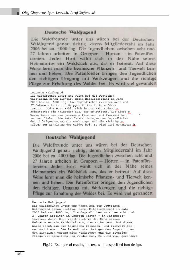
Oleg Choporov, Igor Lvovich, Juraj Štefanovič
108
Fig.12. Example of reading the text with unspecified font design.

Implementation and Testing of Text Recognition Algorithm on Mobile Devices
109
Fig.13. Example of reading text in Times New Roman format.
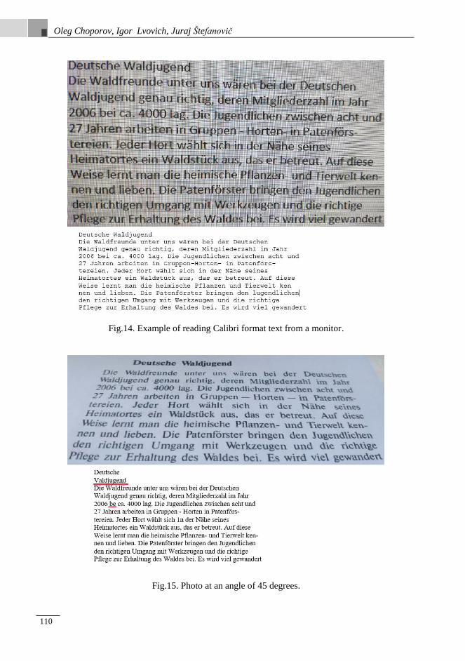
Oleg Choporov, Igor Lvovich, Juraj Štefanovič
110
Fig.14. Example of reading Calibri format text from a monitor.
Fig.15. Photo at an angle of 45 degrees.

Implementation and Testing of Text Recognition Algorithm on Mobile Devices
111
Insufficient illumination was created in 2 stages, from light to darker. In the first example of
(Fig.16), you can see that the image in the photo has become darker by 40%. Despite this fact, the
application did a pretty good job with its task, making only one mistake, missing the letter “f” in the
last line. The error in recognition was 1.0.18%, the accuracy was 99.82%.
If the light source is dimmed even more, thereby making the photo even 30% darker, then the
application starts noticeable problems. It is strikingly more difficult for the system to identify the text
on the image, as a result of which, in the second part of (Fig.16), we see a large number of errors,
namely 11, which is an error of 1.93%. But despite a small percentage of errors, the system incor-
rectly distributes the string order and tears up some sentences, skipping letters, into several lines.
Because of the dark background, it is difficult for him to determine the line boundaries.
At the final stage of testing, a photo was taken with sufficient lighting, but from a crumpled
paper source, an example is shown in (Fig.17). This method distorts the order of the letters, relative
to their original position. These conditions should complicate text recognition. Despite the compli-
cated conditions created, the system was mistaken only 4 times. Inaccuracy was made in the follow-
ing situations: the “-” sign was missed, the letter “ä” was recognized incorrectly and replaced with
“a”, an error in the letter “d” that appeared as “J”, the letter “f” was omitted. It can be concluded that
a crumpled paper source does not greatly affect the operation of the application. The percentage of
errors in the recognition of the text was 0.7%, the accuracy of the process was 99.3%.
After all the planned stages have been completed, a final conclusion can be made on the basis
of the tests performed. The accuracy of recognition is directly dependent on the quality of the image.
One of the key factors for a successful photo is a high-quality light source. The decrease in
the light level in the photograph led to a significant deterioration in recognition accuracy. If under
comfortable conditions the application can read the text with an accuracy of 100%, then when the
light is reduced by 40%, this Picture drops to 99.82%. With a decrease in illumination indicators by
another 30%, the accuracy drops to 98.07%, which is a record low for all the tests performed. It is
also clearly seen that under these conditions, the application copes worse with the positioning of lines
in the text.
Changing the angle of inclination, while maintaining a sufficient light source, did not greatly
affect the quality of recognition. Deformed paper source, too, is not critical. The results were very
similar. In the first case, 3 errors, in the second 4, respectively. Recognizing the test from a photo-
graph on the monitor screen showed that even with large interference, the application can perform
its functionality with an accuracy of up to 100% without making a single mistake.
If you create the right conditions for the application, despite the different text formats and
their sources, it can show the result with an accuracy of up to 100%.
After analyzing the general statistics (an example is given in Table 1), the result shows that
the application does much worse in stressful situations than in ordinary ones. But regardless of the
simulated situations remains relevant for use, and the accuracy in the recognition of the text does not
fall below the mark of 98%.

Oleg Choporov, Igor Lvovich, Juraj Štefanovič
112
Fig.16. Photography with low light.

Implementation and Testing of Text Recognition Algorithm on Mobile Devices
113
Fig.17. Crumpled paper source.
Table 1. Statistics of the results in all simulated situations
Ordinary conditions
Attempt Accuracy bias Errors
Free text 1 99.3% 0.7% 4
2 100% 0% 0
Times New Roman 1 99.65% 0.35% 2
2 100% 0% 0
Calibri 1 100% 0% 0
Stress test
Attempt Accuracy bias Errors
Incline 45О 1 99.47% 0.53% 3
fogging 1 99.82% 0.18% 1
2 98.07% 1.93% 11
Deformation 1 99.3% 0.7% 4

Oleg Choporov, Igor Lvovich, Juraj Štefanovič
114
Conclusion
As a result of this work, an application for phones based on the Android OS has been devel-
oped to create DOC files in which the text obtained from the image is written.
All the previously set conditions for the development of the application have been met,
namely:
1. The analysis is carried out and existing text recognition methods are analyzed.
2. Analysis and analysis of existing API and text recognition methods. Selected the most
suitable and integrated into the application.
3. An algorithm for creating and storing a file in the memory of a mobile device has been
developed and implemented.
4. An algorithm has been developed and implemented that will allow you to receive files
created by an application from a mobile phone. Implemented the ability to send them.
5. Designed and implemented application interface.
6. Tested application.
The mobile application has the following functionality:
- The user has the ability to create documents from the image.
- You can create an image using the camera of the phone or download them
from the device’s memory.
- The user independently enters the name of the created document.
- The application saves a DOC file in the phone memory.
- Implemented the ability to view a list of created documents.
- It is possible to work with the created files and send them through the functions
of the Android OS.
References
[1] Lvovich I. Ya., Lvovich Ya. E., Mozgovoy A. A., Preobrazhensky A. P., Choporov O. N. (2016)
Reduction of errors in recognition of scanned handwritten texts. Digital signal processing. No. 4.
P. 43-47.
2 Vinokurov A.V. (2019) Features of the use of reactivex technology in mobile applications for the
Android operating system. Bulletin of Voronezh Institute of high technologies. № 1(28). P. 53-57.
3 Preobrazhensky A. P., Mozgovoy A. A. (2016) Normalization of images of handwritten words be-
fore recognition. Modeling, optimization and information technologies. № 1 (12). P.6.
[4] Lvovich I. Ya., L. I. E., Mozgovoy A. A., Preobrazhensky A. P., Choporov O. N. (2016) Improv-
ing of algorithm of recognition of handwritten texts on the basis of the valuation of the image.
Modeling, optimization and information technologies. № 3 (14). P.11.
[5] Golovinov S. O., Mironchenko S. G., Shchepilov E. V., Preobrazhensky A. P. (2009) Digital sig-
nal processing. Bulletin of Voronezh Institute of high technologies. No. 4. P. 064-065.

Implementation and Testing of Text Recognition Algorithm on Mobile Devices
115
Authors
Prof. Oleg Choporov
Doctor of Sciences (Engineering), professor
Voronezh state technical university
Prof. Igor Lvovich
Doctor of Sciences (Engineering), professor
Voronezh Institute of High Technologies
Ing. Juraj Štefanovič, PhD.
Faculty of Informatics, Pan-European University, Bratislava, Slovakia

Oleg Choporov, Igor Lvovich, Juraj Štefanovič
116

Information Technology Applications (ITA)
117
List of Reviewers
Issue 1/2019, in alphabetic order
Azarnova, T.V. - Voronezh State University, Russia
Barabanov, V.F. - Voronezh State Technical University, Voronezh, Russia
Beletskaya, S.Yu. - Voronezh State Technical University, Russia
Cigánek, J. - Slovak University of Technology in Bratislava, Slovakia
Drahoš, P. - Slovak University of Technology in Bratislava, Slovakia
Kashirina, I.L. - Voronezh State University, Russia
Kozák, Š. - Pan-European University in Bratislava, Slovakia
Ledeneva, T.M. - Voronezh State University, Voronezh, Russia
Novoseltsev, V.I. - Voronezh Institute of the Federal Penitentiary Service, Russia
Rosinová, D. - Slovak University of Technology in Bratislava, Slovakia
Sakharov, Y.S. - International University of Nature, society and Man „Dubna“ - Moscow
