International Journal of Heat and Mass Transfer 87 (2015) 418–428

Contents lists available at ScienceDirect

International Journal of Heat and Mass Transfer

journal homepage: www.elsevier .com/locate / i jhmt

Temperature-aware time-varying convection over a duty cyclefor a given system thermal-topology

http://dx.doi.org/10.1016/j.ijheatmasstransfer.2015.04.0110017-9310/� 2015 Elsevier Ltd. All rights reserved.

⇑ Corresponding author. Tel.: +1 (778) 782 8538; fax: +1 (778) 782 7514.E-mail addresses: mfakoorp@sfu.ca (M. Fakoor-Pakdaman), mahmadi@sfu.ca

(M. Ahmadi), mbahrami@sfu.ca (M. Bahrami).

M. Fakoor-Pakdaman, Mehran Ahmadi, Majid Bahrami ⇑Laboratory for Alternative Energy Conversion (LAEC), School of Mechatronic Systems Engineering, Simon Fraser University, Surrey, BC, V3T 0A3, Canada

a r t i c l e i n f o a b s t r a c t

Article history:Received 28 September 2014Received in revised form 2 April 2015Accepted 2 April 2015Available online 24 April 2015

Keywords:ConvectionDynamic systemsTransientExperimentDuty cycle

Smart dynamic thermal management (SDTM) is a key enabling technology for optimal design of theemerging transient heat exchangers/heat sinks associated with advanced power electronics and electricmachines (APEEM). The cooling systems of APEEM undergo substantial transition as a result of time-varying thermal load over a duty cycle. Optimal design criteria for such dynamic cooling systems shouldbe achieved through addressing internal forced convection under time-dependent heat fluxes.Accordingly, an experimental study is carried out to investigate the thermal characteristics of a laminarfully-developed tube flow under time-varying heat fluxes. Three different transient scenarios areimplemented under: (i) step; (ii) sinusoidal; and (iii) square-wave time-varying thermal loads. Basedon the transient energy balance, exact closed-form relationships are proposed to predict the coolant bulktemperature over time for the aforementioned scenarios. In addition, based on the obtained experimentaldata and the methodology presented in Fakoor-Pakdaman et al. (2014), semi-analytical relationships aredeveloped to calculate: (i) tube wall temperature; and (ii) the Nusselt number over the implementedduty cycles. It is shown that there is a ‘cut-off’ angular frequency for the imposed power beyond whichthe heat transfer does not feel the fluctuations. The results of this study provide the platform for temper-ature-aware dynamic cooling solutions based on the instantaneous thermal load over a duty cycle.

� 2015 Elsevier Ltd. All rights reserved.

1. Introduction are conservatively designed for a nominal steady-state or worst-

Smart dynamic thermal management (SDTM) is a transforma-tive technology for efficient cooling of advanced power electronicsand electric machines (APEEM). APEEM has applications in:(i) emerging cleantech systems, e.g., powertrain and propulsionsystems of hybrid/electric/fuel cell vehicles (HE, E, FCV) [1,2]; (ii)sustainable/renewable power generation systems (wind, solar,tidal) [3,4]; (iii) information technology (IT) services (data centers)and telecommunication facilities [5–7]. The thermal load of APEEMsubstantially varies over a duty cycle; Downing and Kojasoy [8]

predicted heat fluxes of 150� 200 ½W=cm2� and pulsed transient

heat loads up to 400 ½W=cm2�, for the next-generation insulatedgate bipolar transistors (IGBTs). The non-uniform and time-varyingnature of the heat load is certainly a key challenge in maintainingthe temperature of the electronics within its safe and efficientoperating limits [9]. As such, the heat exchangers/heat sinksassociated with APEEM operate periodically over time and neverattain a steady-state condition. Conventionally, cooling systems

case scenarios, which may not properly represent the thermalbehavior of various applications or duty cycles [10]. The state-of-the-art approach is utilizing SDTM to devise a variable-capacitycooling infrastructure for the next-generation APEEM and the asso-ciated engineering applications [7]. SDTM responds to thermalconditions by adaptively adjusting the power-consumption profileof APEEMs on the basis of feedback from temperature sensors [5].Therefore, supervisory thermal control strategies can then beestablished to minimize energy consumption and safeguard ther-mal operating conditions [9]. As such, the performance of transientheat exchangers is optimized based on the system ‘‘thermal topol-ogy’’, i.e., instantaneous thermal load (heat dissipation) over a dutycycle. For instance, utilizing SDTM in designing the cooling systemsof a data center led to significant energy saving, up to 20%, com-pared to conventionally cooled facility [7]. In addition, in case ofthe HE/E/FCV, SDTM improves the vehicle overall efficiency,reliability and fuel consumption as well as reducing the weightand carbon foot print of the vehicle [11].

Therefore, there is a pending need for an in-depth understand-ing of instantaneous thermal characteristics of transient coolingsystems over a given duty cycle. However, there are only a fewanalytical/experimental studies in the open literature on this topic.

Nomenclature

a heat flux amplitude, ½W=m2�cp heat capacity, ½J=kg=K�cn coefficients in Eq. (10)D tube diameter, ½m�Fo Fourier number, ¼ at=R2

h heat transfer coefficient, ½W=m2=K�J Bessel functionk thermal conductivity, ½W=m=K�L length, ½m�m integer number, Eq. (21)_m mass flow rate, ½kg=s�

NuD local Nusselt number, ¼ ½hðx; tÞ � D�=k

NuD average Nusselt number, 1L2

R L20 NuDdx

P power, ½W�p period of the imposed power, ½s�Pr Prandtl number, ¼ m=aq00 thermal load (heat flux), ½W=m2�R tube radius, ½m�r radial coordinate measured from tube centerline, ½m�Re Reynolds number, ¼ UD=tT temperature, ½K�t time, ½s�U velocity, ½m=s�X dimensionless axial distance, ¼ 4x=Re � Pr � Dx axial distance from the entrance of the heated section, ½m�

Greek lettersa thermal diffusivity, ½m2=s�m kinematic viscosity, ½m2=s�q fluid density, ½kg=m3�kn Eigenvalues in Eq. (10)Kn values defined in Eq. (10)h dimensionless temperature, ¼ T�Tin

q00r D=kW a function defined in Eq. (23)! a function defined in Eq. (18)bn positive roots of the Bessel function, J1ðbnÞ ¼ 0x1 angular frequency of the sinusoidal heat flux,

¼ ð2pR2Þ=ðp1aÞxm dimensionless number characterizing the square-wave

heat flux, ¼ ½ð2mþ 1ÞpR2�=ðp2aÞ

Subscripts1 sinusoidal scenario2 square-wave scenarioin inletm mean or bulk valueout outletr reference valuew wall

Table 1Summary of existing literature on convection under dynamically varying thermalload.

Author Notes

Siegel [12] U Reported temperature distribution inside a circulartube and between two parallel plates� Limited to step wall heat flux� Limited to slug flow condition� Limited to an analytical-based approach withoutvalidation/verification

Siegel [15] U Reported temperature distribution inside a circulartube or between two parallel platesU Covered thermally developing and fully-developedregionsU Considered fully-developed velocity profile� Limited to step wall temperature� Nusselt number was defined based on the tube walland inlet fluid temperature� Limited to an analytical-based approach withoutvalidation/verification

Fakoor-Pakdamanet al. [20]

U Reported temperature distribution inside a circulartubeU Defined the Nusselt number based on the tube walland fluid bulk temperature� Limited to slug flow condition� The analytical results were only verified numerically

Fakoor-Pakdamanet al. [22]

U Reported temperature distribution inside a circulartubeU Considered transient velocity profile for the fluidflow� Limited to sinusoidal wall heat flux.� The analytical results were only verified numerically

M. Fakoor-Pakdaman et al. / International Journal of Heat and Mass Transfer 87 (2015) 418–428 419

This study is focused on transient internal forced convection as themain representative of the thermal characteristics of dynamic heatexchangers under arbitrary time-varying heat fluxes. In fact, suchanalyses lead to devising ‘‘temperature-aware’’ cooling solutionsbased on the system thermal topology (power management) overa given duty cycle. The results of this work will provide a platformfor the design, validation and building new smart thermal manage-ment systems that can actively and proactively control the coolingsystems of APEEMs and similar applications.

1.1. Present literature

Siegel [12–17] pioneered study on transient internal forced-convective heat transfer. Siegel [12] studied laminar forced convec-tion heat transfer for a slug tube-flow where the walls were given astep-change in the heat flux or alternatively a step-change in thetemperature. Moreover, the tube wall temperature of channel slugflows for particular types of position/ time-dependent heat fluxeswas studied in the literature [17,18]. Most of the pertinent litera-ture was done for laminar slug flow inside a duct. The slug flowapproximation reveals the essential physical behavior of the sys-tem, while it enables obtaining exact mathematical solution forvarious boundary conditions. Using this simplification, one canstudy the effects of various boundary conditions on transient heattransfer without tedious numerical computations [12,15]. Siegel[15] investigated transient laminar forced convection with fullydeveloped velocity profile following a step change in the wall tem-perature. The obtained solution was much more complex than theresponse for slug flow which was presented in [12]. It was reportedthat the results for both slug and fully-developed flows showed thesame trends; however, the slug flow under-predicted the tube walltemperature compared to the Poiseuille flow case. Fakoor-Pakdaman et al. [19–22] conducted a series of analytical studieson the thermal characteristics of internal forced convection overa duty cycle to reveal the thermal characteristics of the emergingdynamic convective cooling systems. Such thermal characteristics

were obtained for steady slug flow under: (i) dynamic thermal load[19,20]; (ii) dynamic boundary temperature [21]; and (iii)unsteady slug flow under time-varying heat flux [22]. Most litera-ture on this topic is analytical-based; a summary is presented inTable 1.

Fig. 1. Schematic view of the fabricated experimental setup.

Table 2Summary of calculated experimental uncertainties.

Primary measurements Derived quantities

Parameter Uncertainties Parameter Uncertainties (%)

_m 6% Re 7.6P ½W� 3% h ½W=m2=K� 8.1

TðTin; Tout ; TmÞ 0:5½�C� Nu 8.3

420 M. Fakoor-Pakdaman et al. / International Journal of Heat and Mass Transfer 87 (2015) 418–428

Our literature review indicates:

� There is no experimental work on transient internal forced-convection over a duty cycle under a time-varying thermal load.� The presented models in literature for internal flow under

dynamic thermal load are limited to slug flow conditions.� No analytical model exists to predict the thermal characteristics

of fully developed flow over a harmonic duty cycles.

Although encountered quite often in practice, the unsteadyconvection of fully-developed tube flow under time-varyingthermal load over a duty cycle has never been addressed in litera-ture; neither experimentally nor theoretically. In other words, theanswer to the following question is not clear: ‘‘how the thermalcharacteristics of emerging dynamic cooling systems vary over aduty cycle under time-varying thermal loads (heat fluxes) of theelectronics and APEEM?’’.

An experimental testbed is fabricated to investigate the thermalcharacteristics of a fully-developed tube flow under different tran-sient scenarios: (i) step; (ii) sinusoidal; and (iii) square-wave heatfluxes. Based on the transient energy balance, exact closed-formrelationships are proposed to predict the fluid bulk temperatureunder the studied transient scenarios (duty cycles). The accuracyof the experimental data is also verified by the obtained resultsfor the fluid bulk temperature. Based on the obtained experimentaldata and the methodology presented in [13,18], semi-analyticalrelationships are developed to calculate the: (i) tube wall temper-ature; and (ii) the Nusselt number over the studied duty cycles.Moreover, easy-to-use relationships are presented as the short-time asymptotes for tube wall temperature and the Nusselt num-ber for the case of step wall heat flux. At early times, Fo < 0:2, suchasymptotes deviate only slightly from the obtained series solutionsas the short-time responses; maximum deviation less than 2%.

2. Real-time data measurement

2.1. Experimental setup

The experimental setup fabricated for this work is shownschematically in Fig. 1. The fluid, distilled water, flows down froman upper level tank and enters the calming section. Adjusting theinstalled valves, the water level inside the upper-level tank ismaintained constant during each experiment to attain the desiredvalues of the constant flow during each experiment.

Following [23], the calming section is long enough so thatthe fluid becomes hydrodynamically fully-developed at thebeginning of the heated section. A straight copper tube with12:7� 0:02 ½mm� outer diameter, and 11:07� 0:02 ½mm� innerdiameter is used for the calming and heated sections. The lengthof the former is L1 ¼ 500 ½mm�, while the heated section isL2 ¼ 1900 ½mm� long. Two flexible heating tapes, STH seriesOmega, are wrapped around the entire heated section. Four T-typethermocouples are mounted on the heated section at axial posi-tions in [mm] of T1(300), T2(600), T3(1000), and T4(1700) fromthe beginning of the heated section to measure the wall tempera-ture. In addition, two T-type thermocouples are inserted into theflow at the inlet and outlet of the test section to measure the bulktemperatures of the distilled water. The heating tapes are con-nected in series, while each is 240 ½V� and 890 ½W�. To apply thetime-dependent power on the heated section, two programmableDC power supplies (Chroma, USA) are linked in a master and slavefashion, and connected to the tape heaters. The maximum possiblepower is 300 ½W�. To reduce heat losses towards the surroundingenvironment, a thick layer (5 [cm]) of fiber-glass insulating blanketis wrapped around the entire test section including calming andheated sections. After the flow passes through the test section,

the flow rate is measured by a precise micro paddlewheel flowmeter, FTB300 series Omega. Finally, the fluid returns to the surgetank which is full of ice-water mixture. As a result, the fluid iscooled down, and then is pumped to the main tank at the upperlevel. All the thermocouples are connected to a data acquisitionsystem composed of an SCXI-1102 module, an SCXI-1303 terminaland an acquisition board; all these components are from NationalInstrument. The programmable DC power supplies are controlledvia standard LabVIEW software (National Instrument), to applythe time-dependent powers. As such, different unsteady thermalduty cycles are attained by applying three different scenarios forthe imposed power: (i) step; (ii) sinusoidal; and (iii) square-wave.As such, real-time data are obtained for transient thermal charac-teristics of the system over such duty cycles; see Section 2.2 formore detail. The accuracy of the measurements and the uncertain-ties of the derived values are given in Table 2.

2.2. Data processing

In most Siegel works [13,18], the transient thermal behavior ofa system is evaluated based on the dimensionless wall heat fluxconsidering the difference between the local tube wall and the ini-tial fluid temperature. We are of the opinion that an alternativedefinition of the local Nusselt number has a more ‘physical’ mean-ing, i.e., based on the local difference between the channel wall andthe fluid bulk temperature at each axial location; this is consistentwith [24,25]. It should be emphasized that the definition of theNusselt number is an arbitrary choice and will not alter the finalresults. As such, the overall transient convective heat transfercoefficient is defined as follows:

M. Fakoor-Pakdaman et al. / International Journal of Heat and Mass Transfer 87 (2015) 418–428 421

hðL2; tÞ ¼q00ðtÞ

TwðtÞ � TmðtÞð1Þ

where q00ðtÞ is the applied time-dependent heat flux, TwðtÞ is theaverage tube wall temperature, and TmðtÞ is the arithmetic averageof inlet and outlet fluid bulk temperatures. Therefore, the defini-tions of different parameters in Eq. (1) are given below:

TwðtÞ ¼14

X4

i¼1

TiðtÞ ð2Þ

TmðtÞ ¼TinðtÞ þ ToutðtÞ

2ð3Þ

q00ðtÞ ¼ PðtÞpDL2

ð4Þ

where Tin and Tout are the inlet and outlet fluid temperatures,respectively. Moreover, PðtÞ is the applied transient power and L2

is the length of the heated section. The overall Nusselt number isalso obtained by the following relationship.

NuDðL2; tÞ ¼hðL2; tÞ � D

kð5Þ

where, D and k are the tube diameter and fluid thermal conductiv-ity, respectively. The thermo-physical properties of the distilledwater used in this study are determined at the arithmetic averagetemperature, TmðtÞ, from [23].

3. Model development

In this section, it is intended to present closed-form solutions forthe thermal characteristics of laminar tube flow under the transientscenarios, i.e., (i) step; (ii) sinusoidal; and (iii) square-wave heatfluxes. Following Siegel [13] and Fakoor-Pakdaman et al. [20,22],closed-form relationships are obtained to calculate: (i) tube walltemperature; (ii) fluid bulk temperature; and (iii) the Nusseltnumber, for the above-mentioned time-dependent heat fluxes.

The methodology presented in [13] proceeds as follows: con-sider a position x in the channel through which the fluid is flowingwith average velocity U. A fluid element starting from the entranceof the channel will require time duration t ¼ x=U to reach the xlocation. In the region where x=U P t, i.e., short-time response,there is no penetration of the fluid which was at the entrance whenthe transient began. Therefore, the short-time response corre-sponds to pure transient heat conduction, and the effect of heatconvection is zero. However, for the region x=U 6 t, the heat trans-fer process occurs via the fluid that entered the channel after thetransient was initiated. This forms the long-time response whichis equal to short time response at the transition time, i.e.,t ¼ x=U. Therefore, the solution composed of two parts that shouldbe considered separately: (i) short-time and (ii) long-timeresponses. More detail regarding the short- and long-timeresponses were presented elsewhere [19–22].

3.1. Step power (heat flux)

For this scenario, the imposed heat flux is considered in thefollowing form:

q00ðtÞ ¼0 t < 0q00r ¼ const: t P 0

�ð6Þ

where q00r (offset), is a constant value over the entire heating period.When a tube flow is suddenly subjected to a step heat flux, theshort-time response for the tube wall temperature is obtained asfollows [12]:

hw ¼ Foþ 18�X1n¼1

e�b2nFo

b2n

ð7Þ

where bn are the positive roots of J1ðbÞ ¼ 0, and J1ðbÞ are the first-order Bessel functions of the first kind, respectively. In addition,hw and Fo are the dimensionless wall temperature and dimension-less time, respectively. Such dimensionless numbers are definedas follows:

hw ¼Tw � Tin

q00r D=k; Fo ¼ at

R2 ð8Þ

where Tw; Tin; k, and a are tube wall temperature, inlet tempera-ture, fluid thermal conductivity, and diffusivity, respectively. Itshould be noted that when Fo! 0, Fakoor-Pakdaman andBahrami [26], presented a compact easy-to-use relationship forEq. (7) as the short-time asymptote for the tube wall temperature.For Fo < 0:2, the maximum deviation between the series solution,Eq. (7), and the compact model, Eq. (9), is less than 2%.

hw;Fo!0 ¼ffiffiffiffiffipFo

r� p

4

� ��1

ð9Þ

In addition, the long-time asymptote can be obtained by a well-known Graetz solution [25] as given below:

hw ¼ X þ 1148þ 1

2

X1n¼1

CnKn exp � k2nX2

!ð10Þ

where X ¼ 4x=DRe�Pr is the dimensionless axial location. Besides, the val-

ues of kn and CnKn are tabulated in [25]. In addition, the fluid bulktemperature can be obtained by performing a heat balance on aninfinitesimal differential control volume of the flow;

_mcpTm þ q00ðpDÞdx� _mcpTm þ _mcp@Tm

@xdx

� �¼ qcp

pD2

4

!@Tm

@tdx

ð11Þ

where _m is the fluid mass flow rate, cp and Tm are specific heat andfluid bulk temperature, respectively. The dimensionless form ofEq. (11) is:

q00ðX; FoÞq00r

¼ @hm

@Foþ @hm

@Xð12Þ

where q00r is the offset around which the imposed heat flux fluctu-ates. Eq. (12) is a first-order partial differential equation whichcan be solved by the method of characteristics [27]. The short-and long-time asymptotes for the fluid bulk temperature for thecase of step heat flux are [26];

hm ¼Fo short� time asymptoteX Long� time asymptote

�ð13Þ

Following Fakoor-Pakdaman and Bahrami [26], the short-timeasymptote for the average Nusselt number under a step heat fluxcan be calculated by a compact relationship, Eq. (14).

NuDðtÞFo!0 ¼hðtÞ � D

k¼

ffiffiffiffiffipFo

rð14Þ

In addition, the following well-known Shah equation [28] is used asthe long-time asymptote for the average Nusselt number of laminarflow under constant wall heat flux.

Nu0�x;D ¼1:953X�1=3 for X 6 0:034:364þ 0:0722

X for X > 0:03

(ð15Þ

422 M. Fakoor-Pakdaman et al. / International Journal of Heat and Mass Transfer 87 (2015) 418–428

3.2. Sinusoidal power (heat flux)

For this case, the applied heat flux is considered in the followingform.

q00 ¼ q00r þ a� sin2pp1

t� �

ð16Þ

where, q00r ½W=m2�, a ½W=m2�, and p1 ½s� are the offset, amplitude,and period of the imposed heat flux. The dimensionless form ofEq. (16) is:

q00

q00r¼ 1þ a

q00r

� �� sinðx1FoÞ ð17Þ

where, x1 ¼ 2pR2

p1ais the dimensionless angular frequency of the

imposed heat flux, and R ½m� is the tube radius. SubstitutingEq. (17) into Eq. (12), closed-form relationships are obtained forthe short- and long-time responses for fluid bulk temperature, seeEqs. (18.a) and (18.b). In addition, following the methodology pre-sented in [20], semi-analytical relationships are proposed to predictthe tube wall temperature, Eqs. (19.a) and (19.b). Table 3 presents asummary of the results obtained for short- and long-time responsesof tube wall and fluid bulk temperatures under a sinusoidal heatflux. It should be noted that C1 in Eqs. (19.a) and (19.b), is a coeffi-cient which depends on the velocity profile of the fluid inside thetube. It takes the value of unity for slug flow inside the duct, i.e.,uniform velocity across the tube, see [20]. For a parabolic velocityprofile (poiseuille flow), the value of such coefficient is obtainedin this study empirically, and will be discussed in Section 4, wherethe functions !1;n and !2;n are defined as:

!1;n¼ e�b2n Fo

b2nþx1ða=q00r Þ

x21þb4

n� cosðx1FoÞ� b2

nx1�sinðx1FoÞ�e�b2

n Foh i

!2;n¼ e�b2n X

b2nþx1 ða=q00r Þ

x21þb4

n� cosðx1FoÞ� b2

nx1�sinðx1FoÞþe�b2

n X �b2

nx1�sin x1ðFo�XÞ½ ��

cos½x1ðFo�XÞ�

( )( )8>>><>>>:

ð18Þ

In addition, the short- and long-time local Nusselt numbers can becalculated by the following relationship:

Table 3Tube wall and fluid bulk temperatures for transient scenario II: sinusoidal heat flux, [20].

Short-time response, X 6 Fo

Fluid bulk temperature, hm ¼ Tm�Tinq00r D=k

¼ Foþ a=q00rð Þx1

1� cosðx1FoÞ½ � (18.a)

Tube wall temperature, hw ¼ Tw�Tinq00r D=k

¼ C1Foþ a=q00rð Þ

x1� 1� cosðx1FoÞ½ �

þ 18�

P1n¼1!1;n

( )(19.a)

Table 4Tube wall and fluid bulk temperatures for transient scenario III: square-wave heat flux, R

Short-time response, X 6 Fo

Fluid bulk temperature, hm ¼ Tm�Tinq00r D=k

¼ X þ aq00r

�P1

m¼0;1;21

xmð2mþ1Þcos xmðFo� XÞ½ �� cosðxmFoÞ

� �(25.a)

Tube wall temperature, hw ¼ Tw�Tinq00r D=k

¼ C2

Foþa=q00r� �

�P1

m¼0;1;21

xmð2mþ1Þ �1� cosðxmFoÞ

� �þ 1

8�P1

n¼1W1;n

8>><>>:

9>>=>>; (26.a)

NuDðx; tÞ ¼q00D=k

Tw � Tm¼ C2

1þ sinðx1FoÞhw � hm

� �ð19Þ

Again C2 is a coefficient which takes a value of unity for slug flowinside the duct [20]. The value of such coefficient for a parabolicvelocity in this study is obtained empirically, and discussed inSection 4 of this study. Accordingly, the average Nusselt numberover the entire length of the heated section, L2, is calculated asfollows:

NuDðL2; tÞ ¼1L2

Z L2

0NuDdx ð20Þ

3.3. Square-wave power (heat flux)

The Fourier series for a square-wave heat flux with offset q00r ,amplitude a, and period p2 is, [29]:

q00 ¼ q00r þ a�X1

m¼0;1;2

12mþ 1

sinð2mþ 1Þp

p2t

� �ð21Þ

The dimensionless form of Eq. (21) is:

q00

q00r¼ 1þ a

q00r

� ��X1

m¼0;1;2

12mþ 1

sinðxmFoÞ ð22Þ

where xm ¼ ð2mþ1ÞpR2

p2ais a dimensionless number which character-

izes the behavior of the square-wave heat flux. SubstitutingEq. (22) into Eq. (12), closed-form relationships are obtained forthe short- and long-time responses for fluid bulk temperature, seeEqs. (25.a) and (25.b). In addition, following the methodologypresented in [20], semi-analytical relationships are proposed topredict the tube wall temperature, Eqs. (26.a) and (26.b). Table 4presents a summary of the results obtained for short- and long-timeresponses of tube wall and fluid bulk temperatures under a square-wave heat flux.

Long-time response, X P Fo

¼ X þ a=q00rð Þx1

cos x1ðFo� XÞ½ � � cosðx1FoÞf g (18.b)

¼ C1X þ a=q00rð Þ

x1� cos x1ðFo� XÞ½ �� cosðx1FoÞ

� �þ 1

8�P1

n¼1!2;n

8<:

9=; (19.b)

ef. [20].

Long-time response, X P Fo

¼ X þ aq00r

�P1

m¼0;1;21

xmð2mþ1Þcos xmðFo� XÞ½ �� cosðxmFoÞ

� �(25.b)

¼ C2

Xþa=q00rð Þxm�P1

m¼0;1;21

xmð2mþ1Þ �cos xmðFo� XÞ½ �� cosðxmFoÞ

� �þ 1

8�P1

n¼1W2;n

8>><>>:

9>>=>>; (26.b)

Fig. 2. Short- and long-time asymptotes for outlet fluid bulk-temperature and comparison with experimental data for the step power. ð _m ¼ 3:3� 0:198 ½gr=s�Þ.

Fig. 3. Short- and long-time responses for outlet fluid bulk temperature and comparison with experimental data for the square-wave power. ð _m ¼ 3:6� 0:216 ½gr=s�Þ.

M. Fakoor-Pakdaman et al. / International Journal of Heat and Mass Transfer 87 (2015) 418–428 423

The functions W1;n and W2;n are defined as:

W1;n ¼ e�b2n Fo

b2nþða=q00r Þ�

X1m¼0;1;2

xm

ð2mþ1Þðx2mþb4

n Þ� cosðxmFoÞ� b2

nxm� sinðxmFoÞ�e�b2

n Foh i

W2;n ¼ e�b2n X

b2nþða=q00r Þ�

X1m¼0;1;2

xm

ð2mþ1Þðx2mþb4

n Þ�

cosðxmFoÞ� b2n

xm� sinðxmFoÞþ

e�b2n X �

b2n

xm� sin½xmðFo�XÞ��

cos½xmðFo�XÞ�

( )8>><>>:

9>>=>>;

8>>>>>>>><>>>>>>>>:

ð23Þ

In addition, the short- and long-time local Nusselt numbers can beobtained by the following relationship:

NuDðx; tÞ ¼q00D=k

Tw � Tm

¼ C2

1þ aq00r

�P1

m¼0;1;21

2mþ1 sinðxmFoÞhw � hm

24

35 ð24Þ

Similar to Section 3.2, the average Nusselt number over the entirelength of the heated section is:

NuDðL2; tÞ ¼1L2

Z L2

0NuDdx ð25Þ

Fig. 4. Short- and long-time responses for outlet temperature and comparison with experimental data for sinusoidal power with different periods: (a) p1 ¼ 400 ½s� and (b)p1 ¼ 50 ½s�. ð _m ¼ 3:6� 0:216 ½gr=s�Þ.

424 M. Fakoor-Pakdaman et al. / International Journal of Heat and Mass Transfer 87 (2015) 418–428

4. Results and discussion

4.1. Validation tests/outlet fluid bulk-temperature

Fig. 2 shows the dimensionless short- and long-time asymp-totes, Eq. (13), for the outlet fluid bulk-temperature against thedimensionless time (Fourier number) for a step power. The exactanalytical results are also compared with the obtained experimen-tal data in Fig. 2.

The following highlights the trends in Fig. 2:

� There is an excellent agreement between the exact analyticalsolutions and the obtained experimental data. The maximumrelative difference between the derived asymptotes and theexperimental data is less than 8%.

� The good agreement between the analytical results and theexperimental data verifies the accuracy of the experimentalsetup and the measuring instruments.� As the heating is applied, the outlet fluid bulk-temperature

increases to reach the steady-state value at the long-timeasymptote.� The experimental data show a smooth transition between the

short- and long-time responses.

Fig. 3 depicts the variations of dimensionless outlet fluid bulk-temperature against the Fourier number for a square-wave power.The exact analytical results are also compared with the obtainedexperimental data in Fig. 3. The following conclusions can bedrawn from Fig. 3:

M. Fakoor-Pakdaman et al. / International Journal of Heat and Mass Transfer 87 (2015) 418–428 425

� There is a good agreement between the analytical resultsand the obtained experimental data; the maximum relativedifference less than 12%.� The good agreement between the analytical results and the

experimental data verifies the accuracy of the experimentalsetup and the measuring instruments.� As the heating is applied, the temperature of the fluid rises to

show steady oscillatory behavior after the transition time,X ¼ Fo. This time is demarcated on Fig. 3 by a vertical dash line.� There is an initial transient period, which can be considered as

pure conduction, i.e., the short-time response for X P Fo.However, as pointed out earlier, each axial position showssteady oscillatory behavior for X < Fo at the long-time response.� There is a slight discrepancy between the analytical results and

experimental data around the transition time. Referring to[12,20], this happens as a result of the limitations of the math-ematical method ‘‘method of characteristics’’ that is used in [20]to solve the energy equation. Such mathematical method pre-dicts an abrupt transition from short- to long-time responseswhile experimental data show a smooth transition.� As expected the fluid temperature fluctuates with time in case

of a square-wave heat flux. For a step heat flux, the solutiondoes not fluctuate over time. The temperature fluctuates withthe period of the imposed heat flux.

4.2. Cut-off angular frequency

Fig. 4 shows the dimensionless outlet fluid bulk-temperatureversus the Fourier number under a sinusoidal power. To investi-gate the effects of the angular frequency of the applied heat fluxon the coolant behavior, ‘‘slow’’ and ‘‘fast’’ functions are taken intoaccount for the imposed power. Fig. 4a shows a ‘‘slow’’ transientscenario where the angular frequency of the applied power isp1 ¼ 400 ½s�, while the corresponding value in the ‘‘fast’’ case inFig. 4b is p1 ¼ 50 ½s�. The following highlights the trends in Fig. 4:

� There is a shift between the peaks of the applied power andthe outlet fluid bulk-temperature. This shows a ‘‘thermal lag’’(inertia) of the fluid flow. This thermal lag is attributed to thefluid thermal inertia.

Fig. 5. Short- and long-time asymptotes for tube wall temperature and compa

� When a sinusoidal cyclic heat flux with high angular frequencyis imposed on the flow, the fluid does not follow the details ofthe heat flux behavior. Therefore, for very high angular frequen-cies, the fluid flow acts as if the imposed heat flux is constant at‘‘the average value’’ associated with zero frequency for thesinusoidal heat flux.� For high angular frequencies, i.e., p! 0orx!1, the fluid

flow response yields that of a step heat flux. This is called the‘‘cut-off’’ pulsation frequency.� Dimensionless cut-off angular frequency: defined in this

study as the angular frequency beyond which the fluidresponse lies within �5% of that of step heat flux. As such,following [22], for a fully developed tube flow subjected to a

sinusoidal wall heat flux, x1 ¼ 2pR2

p1a¼ 15p is the cut-off angular

frequency.� The dimensionless cut-off frequency is a function of heat flux

period, p1 ½s�, tube radius, R ½m�, and fluid thermal diffusivity,a ½m2

s �.� Irrespective of Fo number, the amplitude of the dimensionless

fluid bulk-temperature decreases remarkably as the angular fre-quency increases. As mentioned earlier, this happens due to thefact that for high angular frequencies the fluid flow responseapproaches to that of the step heat flux.

4.3. Tube wall temperature

Fig. 5 shows variations of short- and long-time asymptotes fortube wall temperature, Eqs. (7) and (10), against the dimensionlesstime (Fourier number). A comparison is also made in Fig. 6between the presented asymptotes, Eqs. (7) and (10), and theobtained experimental data. Step heat flux, Eq. (6), is imposed onthe tube wall and the experimental data are reported for the ther-mocouples T1 and T4 which are corresponding to axial locationsX ¼ 0:15 and 0:4, respectively. The trends for other axial locationsare similar.

The following conclusions can be drawn from Fig. 5:

� As heating is applied, the wall temperature rises and then levelsout at a steady state value, i.e., long-time asymptote.

rison with experimental data for the step power. ð _m ¼ 3:3� 0:198 ½gr=s�Þ.

Fig. 6. Short- and long-time responses for tube wall temperature and comparison with experimental data for: (a) sinusoidal and (b) square-wave power.ð _m ¼ 3:6� 0:216 ½gr=s�Þ.

426 M. Fakoor-Pakdaman et al. / International Journal of Heat and Mass Transfer 87 (2015) 418–428

� There is a good agreement between the experimental data andthe short- and long-time asymptotes, Eqs. (9) and (10); maxi-mum relative difference less than 9.2%.� The obtained experimental data show a smooth transition

between the short- and long-time asymptote.� Around the transition time, the experimental data branch off

from the short-time asymptote and plateau out at the long-timeasymptote, Eq. (10).

Fig. 6 depicts the variations of closed-form solutions and exper-imental results for tube wall temperature over the dimensionlesstime (Fourier number) for: (a) sinusoidal power, Eqs. (19.a) and(19.b); and (b) square-wave power, Eq. (26.a) and (26.b). Theexperimental data are reported for the thermocouples T1 and T3

which are corresponding to X ¼ 0:1 and 0:27, respectively. Thetrends for other axial locations are similar. The following highlightsthe trends in Fig. 6:

� There is an initial transient period of pure conduction, i.e.,short-time response, during which all of the curves follow alongthe same line, X P Fo.� When Fo ¼ X, each curve moves away from the common line, i. e.,

pure conduction response and adjusts towards a steady oscillatorybehavior at long-time response. The transition time for the axiallocations considered in Fig. 6, are indicated by vertical dash lines.� The wall temperatures become higher for larger X values, as

expected, because of the increase in the fluid bulk temperaturein the axial direction.� As mentioned before, the value of C1 is unity for slug flow, while

it should be obtained empirically for other velocity profiles.Based on the obtained experimental data, the value of C1 is con-sidered equal to 1.7; in mathematical notation, C1 ¼ 1:7. Assuch, there is an excellent agreement between the closed-formrelationships Eqs. (16) and (22), and the experimental data overthe short-and long-time responses.

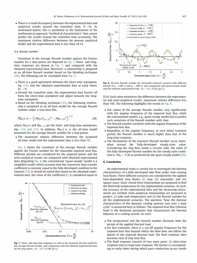
Fig. 8. All-time Nusselt number for sinusoidal transient scenario with differentperiods of p1 ¼ 200 ½s� and p1 ¼ 400 ½s�, and comparison with quasi-steady modeland the obtained experimental data. ð _m ¼ 3:6� 0:216 ½gr=s�Þ.

M. Fakoor-Pakdaman et al. / International Journal of Heat and Mass Transfer 87 (2015) 418–428 427

� There is a small discrepancy between the experimental data andanalytical results around the transition time, X ¼ Fo. Asmentioned before, this is attributed to the limitations of themathematical approach ‘‘method of characteristics’’ that cannotpredict the results around the transition time accurately. Themaximum relative difference between the present analyticalmodel and the experimental data is less than 10.1%.

4.4. Nusselt number

Variations of the average Nusselt number against the Fouriernumber for a step power are depicted in Fig. 7. Short- and long-time responses are shown in Fig. 7, and compared with theobtained experimental data. Moreover, a relationship is proposedas an all-time Nusselt number based on the blending technique[30]. The following can be concluded from Fig. 7:

� There is a good agreement between the short-time asymptote,Eq. (14), and the obtained experimental data at early times,Fo! 0.� Around the transition time, the experimental data branch off

from the short-time asymptote and adjust towards the long-time asymptote.� Based on the blending technique [31], the following relation-

ship is proposed as an all-time model for the average Nusseltnumber under a step heat flux.

NuDðt; xÞ ¼ ½ðNuDðtÞFo!0Þ�3 þ ½Nu0�x;D�3

n oð1=3Þð26Þ

where NuDðtÞ and Nu0�x;D are the short- and long-time asymptotes,Eqs. (14) and (15). In addition, NuDðt; xÞ is the all-time modelpresented for the average Nusselt number for a step power.

� The maximum relative difference between the proposedall-time model and the experimental data is less than 7%.

Fig. 8 shows the variations of the average Nusselt numberagainst the Fourier number for the sinusoidal imposed heat flux.Different periods are considered for the imposed power and thesemi-analytical results are compared with obtained experimentaldata. Regarding Fig. 8, the conventional ‘‘quasi-steady’’ model is asimplified model which assumes that the convective heat transfercoefficient is constant, equal to the fully developed condition in thechannel [13]. It should be noted that based on the obtained exper-imental data, the value of the coefficient C2 is considered equal to

Fig. 7. Short- and long-time responses as well as the proposed all-time model forthe average Nusselt number, and comparison with the obtained experimental datafor the step power. ð _m ¼ 3:3� 0:198 ½gr=s�Þ.

0.54. Such value minimizes the difference between the experimen-tal and semi-analytical results; maximum relative difference lessthan 10%. The following highlights the trends in Fig. 8.

� The values of the average Nusselt number vary significantlywith the angular frequency of the imposed heat flux, whilethe conventional models, e.g., quasi-steady model fail to predictsuch variations of the Nusselt number with time.� The Nusselt number oscillates with the angular frequency of the

imposed heat flux.� Regardless of the angular frequency, at very initial transient

period, the Nusselt number is much higher than that of thelong-time response.� The fluctuations of the transient Nusselt number occur some-

what around the fully-developed steady-state value.Considering the slug flow inside a circular tube, the value ofthe fully-developed Nusselt number for the steady-state condi-tion is: NuD ¼ 4:36 as predicted by the quasi-steady model [25].

6. Conclusion

An experimental study is carried out to investigate the thermalcharacteristics of a fully-developed tube flow under time-varyingheat fluxes. Three different scenarios are considered for the appliedtime-dependent heat fluxes: (i) step; (ii) sinusoidal; and (iii)square-wave. Exact closed-form relationships are proposed to findthe fluid bulk temperature for the implemented scenarios. As such,the accuracy of the experimental data and the measuring instru-ments are verified. Semi-analytical relationships are proposed topredict; (i) tube wall temperature and (ii) the Nusselt number forall the implemented scenarios. The question ‘‘how the thermalcharacteristics of the dynamic cooling systems vary over a dutycycle’’ is answered here as follows: The imposed heat flux (thermalload) is the dominant parameter that characterizes the thermalbehavior of a cooling system. As such;

� The temperature and the Nusselt number fluctuate with theperiod of the applied thermal load.� For fast transients, there is a cut-off angular frequency for the

imposed heat flux beyond which the fluid does not follow thedetails of the imposed thermal load. The fluid response thenbecomes that of step heat flux.� The fluid response consists of two main parts: (i) short-time

response and (ii) long-time response. The former is correspond-ing to early times during which pure conduction occurs inside

428 M. Fakoor-Pakdaman et al. / International Journal of Heat and Mass Transfer 87 (2015) 418–428

the fluid domain. On the other hand, long-time response refersto a period of time starting after the transition time; the fluidyields steady-oscillatory behavior.� The conventional steady-state models fail to predict the thermal

behavior of dynamic cooling systems under time-varying ther-mal load.

Conflict of interest

None declared.

Acknowledgments

This work was supported by Automotive Partnership Canada(APC), Grant No. APCPJ 401826-10. The authors would like to thankthe support of the industry partner, Future Vehicle TechnologiesInc. (British Columbia, Canada).

References

[1] M. Marz, A. Schletz, Power electronics system integration for electric and hybridvehicles, in: 6th Int. Conf. Integr. Power Electron. Syst., 2010, pp. Paper 6.1.

[2] K. Chau, C. Chan, C. Liu, Overview of permanent-magnet brushless drives forelectric and hybrid electric vehicles, IEEE Trans. Ind. Electron. 55 (2008) 2246–2257.

[3] J. Garrison, M. Webber, Optimization of an integrated energy storage schemefor a dispatchable wind powered energy system, in: ASME 2012 6th Int. Conf.Energy Sustain. Parts A B San Diego, CA, USA, 2012, pp. 1009–1019.

[4] J. Garrison, M. Webber, An integrated energy storage scheme for a dispatchablesolar and wind powered energy system and analysis of dynamic parameters,Renew. Sustain. Energy 3 (2011) 1–11.

[5] C. Crawford, Balance of power: dynamic thermal management for Internetdata centers, IEEE Internet Comput. 9 (2005) 42–49.

[6] R.R. Schmidt, E.E. Cruz, M. Iyengar, Challenges of data center thermalmanagement, IBM J. Res. Dev. 49 (2005) 709–723.

[7] Y. Joshi, P. Kumar, B. Sammakia, M. Patterson, Energy Efficient ThermalManagement of Data Centers, Springer, US, Boston, MA, 2012.

[8] R. Scott Downing, G. Kojasoy, Single and two-phase pressure dropcharacteristics in miniature helical channels, Exp. Therm. Fluid Sci. 26 (2002)535–546.

[9] S.V. Garimella, L. Yeh, T. Persoons, Thermal Management Challenges inTelecommunication Systems and Data Centers Thermal ManagementChallenges in Telecommunication Systems and Data Centers, CTRC Res. Publ,2012. pp. 1–26.

[10] M. O’Keefe, K. Bennion, A comparison of hybrid electric vehicle powerelectronics cooling options, in: Veh. Power Electron. Cool. Options, 2007,pp. 116–123.

[11] C. Mi, F.Z. Peng, K.J. Kelly, M.O’. Keefe, V. Hassani, Topology, design, analysisand thermal management of power electronics for hybrid electric vehicleapplications, Int. J. Electr. Hybrid Veh. 1 (2008) 276–294.

[12] R. Siegel, Transient heat transfer for laminar slug flow in ducts, Appl. Mech. 81(1959) 140–144.

[13] R. Siegel, M. Perlmutter, Laminar heat transfer in a channel with unsteady flowand wall heating varying with position and time, Trans. ASME 85 (1963)358–365.

[14] R. Siegel, M. Perlmutter, Heat transfer for pulsating laminar duct flow, HeatTransfer 84 (1962) 111–122.

[15] R. Siegel, Heat transfer for laminar flow in ducts with arbitrary time variationsin wall temperature, Trans. ASME 27 (1960) 241–249.

[16] M. Perlmutter, R. Siegel, Two-dimensional unsteady incompressible laminarduct flow with a step change in wall temperature, Trans. ASME 83 (1961)432–440.

[17] M. Perlmutter, R. Siegel, Unsteady laminar flow in a duct with unsteady heataddition, Heat Transfer 83 (1961) 432–439.

[18] R. Siegel, Forced convection in a channel with wall heat capacity and with wallheating variable with axial position and time, Int. J. Heat Mass Transfer 6(1963) 607–620.

[19] M. Fakoor-Pakdaman, M. Andisheh-Tadbir, M. Bahrami, Transient internalforced convection under arbitrary time-dependent heat flux, in: Proc. ASMESummer Heat Transf. Conf., Minneapolis, MN, USA, 2013.

[20] M. Fakoor-Pakdaman, M. Andisheh-Tadbir, M. Bahrami, Unsteady laminarforced-convective tube flow under dynamic time-dependent heat flux, J. HeatTransfer 136 (2014) 041706.

[21] M. Fakoor-Pakdaman, M. Ahmadi, M. Bahrami, Unsteady internal forced-convective flow under dynamic time-dependent boundary temperature,J. Thermophys. Heat Transfer 28 (2014) 463–473.

[22] M. Fakoor-Pakdaman, M. Ahmadi, M. Andisheh-Tadbir, M. Bahrami, Optimalunsteady convection over a duty cycle for arbitrary unsteady flow underdynamic thermal load, Int. J. Heat Mass Transfer 78 (2014) 1187–1198.

[23] F.P. Incropera, D.P. Dewitt, T.L. Bergman, A.S. Lavine, Introduction to HeatTransfer, fifth ed., John Wiley & Sons, USA, 2007.

[24] Z. Guo, H. Sung, Analysis of the Nusselt number in pulsating pipe flow, Int. J.Heat Mass Transfer 40 (1997) 2486–2489.

[25] A. Bejan, Convection Heat Transfer, third ed., USA, 2004.[26] M. Fakoor-Pakdaman, M. Bahrami, Transient internal forced convection under

step wall heat flux, in: Proc. ASME 2013 Summer Heat Transf. Conf. HT2013,2013.

[27] T. Von Karman, M.A. Biot, Mathematical Methods in Engineering, McGraw-Hill,New York, 1940.

[28] R.K. Shah, Thermal entry length solutions for the circular tube and parallelplates, in: Proceeding 3rd Natl. Heat Mass Transf. Conf., Indian Institute ofTechnology, Bombay, 1975, pp. HMT–11–75.

[29] E. Kreyszig, H. Kreyzig, E.J. Norminton, Advanced Engineering Mathematics,10th ed., John Wiley & Sons, n.d.

[30] S.W. Churchill, R. Usagi, A general expression for the correlation of ratesof transfer and other phenomena, Am. Inst. Chem. Eng. 18 (1972) 1121–1128.

[31] R. Siegel, E.M. Sparrow, Transient heat transfer for laminar forced convectionin the thermal entrance region of flat ducts, Heat Transfer 81 (1959) 29–36.