international journal of computer science,...
TRANSCRIPT
International Journal of Computer Science, Engineering and Applications (IJCSEA) Vol.2, No.4, August 2012
DOI : 10.5121/ijcsea.2012.2404 25
NUMERICAL STUDIES OF TRAPEZOIDALPROTOTYPE AUDITORY MEMBRANE (PAM)
Harto Tanujaya1, Satoyuki Kawano2
1Department of Mechanical Engineering, Tarumanagara University, Jakarta, [email protected]
2Mechanical Science and Bioengineering Department, Osaka University, Japan
ABSTRACT
In this research, we developed numerically a Prototype Auditory Membrane (PAM) for a fully implantableand self contained artificial cochlea. Cochleae are one of the important organs for hearing in the humanand animals. Material of the prototype and implant of PAM are made of Polyvinylidene fluoride (PVDF)-Kureha, Japan which is fabricated using MEMS and thin film technologies. Another important thing in thecharacteristic of the PAM is not only convert the acoustic wave into electric signal but also the frequencyselectivity. The thickness, Young’s modulus and density of the PAM are 40 μm, 4 GPa, and 1.79 103
kg/m3, respectively. The shape and dimension of the PAM is trapezoidal with the width is linearly changedfrom 2.0 to 4.0 mm with the length are 30 mm. Numerically, we develop the model of PAM is based oncommercial CFD software, Fluent 6.3.26 and Gambit 2.4.6. The geometry model of the PAM consists ofone-sided blocks of quadrilateral elements for 2D model and tetrahedral elements for 3 D modelrespectively. In this study we set the flow as laminar and carried out using unsteady time dependentcalculation. The results show that the frequency selectivity of the membrane is detected on the membranesurface.
KEYWORDS
Cochlea, PVDF, PAM, Frequency Selectivity
1. INTRODUCTION
As a medical treatment for sensorineural hearing loss in children and adults, cochlear implant isrecently used [1][2]. The current cochlear implant consist of an implant stimulating electrodesand an extracorporeal device, which bypass the damaged hair cells by generating electric currentin response to the acoustical sound [3]. There is a battery inside the extracorporeal device, whichis one of the critical disadvantages in the current cochlear implant. This status motivates us todevelop a fully self-contained artificial cochlea.
The function and geometrical of the cochlea has been being studied by many researchers in theworld. Measuring and modelling the geometric of the cochlea and biological basilar membranetechnically are very complicated, these become a challenge to be researched. In this research weuse the Prototype Auditory Membrane (PAM) as the simplifying model of the biological basilarmembrane. The important role of the cochlea is not only conversion of acoustical sound to
International Journal of Computer Science, Engineering and Applications (IJCSEA) Vol.2, No.4, August 2012
26
electrical signals but also frequency selectivity [4]. Numerical simulation is one of tools to predictthe frequency selectivity on it. The simulation of fluid flow is an application of numerical methodfor estimating the pattern of fluid flow distribution as well as on cochlea. These methods describethe prediction of fluid flow process and its distribution, before and after a real fluid flow processhappened [5]. The information about fluid flow distribution with certain frequency are utilized tocreate a pressure distribution area map and fluid flow activity. Generally in this research, we havestudied in depth the characteristic of the artificial cochlea. We will report a novel piezoelectricartificial cochlea which works on acoustic wave with frequency selectivity. This system is relatedwith the oscillation and piezoelectric effect. Experimentally, the frequency of the acoustic wave iscontrolled from 1 kHz to 20 kHz, which covers the human audible frequency. The research paperconsists of an introduction as well as a brief description of the research objective, mechanicalmodel and design including results of the numerical simulation.
2. NUMERICAL SIMULATION
In this paper, we develop and simulate the model is based on the numerical method. The model isdeveloped and simulated based on the commercial CFD software, Fluent 6.3.26, and Gambit2.4.6. The Fluent 6.3.26 use finite-volume code, generally this commercial software is used inhydrodynamics and mass transfer computations [6]. The Gambit 2.4.6 is used to provide thecomplete mesh flexibility, and solve the flow problems with both structured and unstructuredmeshes. All functions of the Fluent and Gambit software’s are required to compute a solution anddisplay the results. These software are also accessible either through an interactive interface orconstructed using user-defined-functions (UDS).
The main challenge of the numerically predicting sound waves stems from the well-recognizedfact that sounds have much lower energy than fluid flows, typically by several orders ofmagnitude. This poses a great challenge to the computation of sounds in terms of difficulty ofnumerically resolving sound waves, especially when one is interested in predicting soundpropagation to the far field.
2.1. CFD
At present, Computational Fluid Dynamic (CFD) is a relatively new engineering tool that hasgrown side by side with the development of the computer. CFD has been limited only bycomputer RAM or lack of there, due to the use on billions upon billions of calculations anditerations. Fluent was used in this project, this software was used to simulate flow in very smallduct (MEMS) and determine the pressure that occur in the duct with reasonable accuracy. This iskey to many fields of engineering because duct flows similar to this are used by the medical,automotive, horticultural, and construction industries. As a result, equations and plots can becreated to assist industry in the production of better products.
It is the capability to develop larger and more complex simulations of real world fluidexperiments on computers. Generally, computers can be used to solve FEA stress simulations,simulate fluid flow and heat transfer. Along with computers, the Navier-Stokes equation allowedlarge, complex simulations of fluid flows to be solved. Equations below are the Navier-Stokesequation [7].

International Journal of Computer Science, Engineering and Applications (IJCSEA) Vol.2, No.4, August 2012
27
Surprisingly, this equation was developed in the early nineteenth century by Claude Louis MarieNavier and Sir George Gabriel Stokes. In CFD, the differential equations are used as algebraicequations that describe small finite fluid elements that can then be estimated.
CFD simulation usually includes three steps: preprocessing, processing, and post processing. Forthe preprocessing step, a specific system is identified. The geometry and material propertiesshould be clearly defined, and meshing usually follows after geometry is determined. This isaccomplished by dividing geometry into many small elements or volumes. Meshing in Gambit isa complicated work, as it is critical for both the accuracy of final result and the cost of numericalcalculation. Generally, the finer the divided elements are the closer will be the final solution tothe true value at the expense of more calculation time. The setting of boundary conditions, initialconditions and convergence criteria are also completed in the pre-processing stage. In theprocessing stage, there are iterative calculations in each cell, which are carried out untilconvergence criteria are met. This calculation-intensive process constitutes is the core content ofCFD application. It is not uncommon to have tens of thousands of calculation for even arelatively simple problem. After the completion of processing, the results can be evaluated eithernumerically or graphically. The graphical methods provide a more convenient way to evaluate theoverall effect. This includes signal plot, frequency, vector plot, plot of scalar variables, etc. Thesevisualization tools in post-processing stage allow quick assessment and comparison of calculationresults.
This research utilized a CFD program called Fluent. Fluent and CFD programs make guesses atthe solution and check how accurate the guess until it reaches a user defined “convergence.” Theconvergence term is similar to an error value that results from the computers guess at the Navier-Stokes equation and represents the precision of the simulation. Many of the Navier-Stokesvariables are input by the user such as the inlet pressures, boundaries, outlet types, and fluidproperties. Next, the computer makes a guess at the velocity field for the system and checks theaccuracy of its guess [8].
This cycle is referred to as a iteration. Iterations occur until the computers guesses reach the userdefined convergence point. Once that is accomplished, the user can examine the velocity field forflow rates, pressures, energy transfers, and many other important characteristics. For this project,the pressure into and out of the system was examined. However to use Fluent, a finite elementgrid or mesh of the geometry was needed.
Packaged with Fluent is a program called Gambit. Gambit is a CAD (computer aided design)program that allows a user to generate a model and then section it into small control volumes foruse in Fluent. The accuracy of the Fluent simulations are critically tied to this program becauseGambit is responsible for how many analysis points are placed in the model. Simply, put thehigher number of volumes, because the higher volumes can make more the accurate. This alsohas a down side because with more volumes, comes longer iteration time. Moreover, this cansometimes exceed the computers available memory and computational abilities.
This research explores the behavior of a fluid that is subjected to a force and the flow pattern thatis resulted. Basic mechanisms need to be understood before Fluent can be used because Fluentrequires the user to input the external constraints and set up the simulation environment. Toproduce a fluid flow, a difference in pressure between the inlet and each outlet is required.
International Journal of Computer Science, Engineering and Applications (IJCSEA) Vol.2, No.4, August 2012
28
The governing equations of the sound waves through the duct are the mass continuity equation,equilibrium equation and energy equation. Generally, the equation of motion governs fluid flowis well known as the Navier-Stokes equation. Most researches on fluid dynamics are mostlydedicated to get the solutions of this equation with particular boundary conditions, because ofdifficulties in obtaining exact solutions for this kind of nonlinear equation [9].
The fluid characteristic by two parameters, fluid velocity and fluid density and the behavior offluid flow obeys two laws, for instance the conservation of mass and the conservation ofmomentum. The conservation of mass means the initial and the final masses should remain thesame. Let consider a finite volume (∀) of fluid with A is a closed surface of the finite volume.The mass of fluid using a finite volume is∫ ∀, the mass of fluid through a closed surfaceis∫ ∀. The conservation of mass means that the incoming and outgoing flux of fluid areconserved per unit time in a finite volume.
2.2. Two and Three Dimensional Model of PAM
The grid model of PAM with a basiliar membrane is shown in Figure 1. The PAM is one ofMicroelectomechanical System (MEMS) device. In this study, the frequency selectivity of thePAM can be investigated using computational fluid dynamics (CFD) and structural analysis.Simulation model of the PAM consists of two cochlear ducts both filled with liquid. In the middleof the ducts there is a basilar membrane. The membrane separates the ducts as shown in Figure 1.The shape of basilar membrane is trapezoidal and the mechanical impedance changes along thelongitudinal direction. The acoustic pressure is applied to the liquid from the inlet region, themembrane will be oscillated due to the fluid-structure interaction and it works as a so-calledvariable wave guide. In order to clarify the characteristics of frequency selectivity, the fluid flowand the vibration of the membrane are studied based on the numerical simulation.
We use the 2D and 3D models of the artificial cochlear in this calculation. The inlet position of2D and 3D model are located at side of the membrane, respectively. The flow in the cochlearducts modeled as Newtonian, compressible, laminar and unsteady liquid flow based on theNavier-Stokes equations. Surface of the membranes are treated as non-slip and rigid wall.Equation of state relate the other variables to the two state variables, if we use ρ and T as statevariables we have state equations for pressure p and specific internal energy i, p = p (ρ , T) and i= i (ρ , T), for perfect gas the following, equation of state are useful, p = ρ R T and i = cv T [6].
(1)
The compressible fluid flows, the equations of state provide the linkage between the energyequation on the one hand, and mass conservation and momentum equations on the other. Withoutdensity variation there is no linkage between the energy equation and the mass conservation andmomentum equations. The basic equations are numerically solved using Fluent 6.3.26.
Acoustic pressure pulse applied from the inlet to effectively analyze the response at variousfrequencies. The width and the magnitude of the pulse define are 20 μs and 0.002 Pa,respectively, where the pulse includes waves at all of the audible frequencies from 20 Hz to 20kHz. The spatial distribution of acoustic pressure at a certain frequency obtained from thefrequency spectrum of the acoustic pressure.
gaugeopabs ppp +=TR
pp
o
gaugeop
.
+=

International Journal of Computer Science, Engineering and Applications (IJCSEA) Vol.2, No.4, August 2012
29
The meshing work for the geometry of the duct was done with Gambit 2.4.6 in 3-D analyses. Gridrefinement was performed according to the concentration gradient within the module geometry.The final result represented the result after completing grid refinement and grid independence.The pressure and momentum discretization schemes are second-order accurate, for timeintegration process, first order implicit method used [14].
In this paper, we develop the model of artificial cochlea using plat bending theory and simulationwere based on the commercial CFD software, Fluent 6.3.26 and Gambit 2.4.6. The geometry ofthe duct consist of 1 one-sided blocks of quadrilateral elements for 2D model and tetrahedralelements for 3D model respectively, using map-type mesh and was exported to Fluent®. In thisblock, there are 31,903 nodes, 63,222 faces for 2D model and 188,796 nodes, 2,015,880 faces for3D model. In this study we set the flow as compressible flow and we do not use the turbulenceflow because the exploration times are relatively short. Thus we consider the followingassumptions related to the fluid flow domain, the fluid is a continuous medium, Newtonian,gravity is neglected and the flow is laminar. There are three positions of measurement, inlet,middle and outlet regions as shown in Figure 1 (a) ~ (c).
(a) Trapezoidal Grid Design (b) Basal Grid (c) Apex GridFigure 1 Grid structure (a) Trapezoidal grid design (b) basal grid (c) apex grid
Figure 1 and 2 show the mesh and the grid of the duct model with the basilar membrane in themiddle and center of the cochlear duct.
(a) Part (b) FullFigure 2. Mesh at the center of the duct model (a) part (b) full
The volume statistic for the modeling and simulations are shown,
International Journal of Computer Science, Engineering and Applications (IJCSEA) Vol.2, No.4, August 2012
30
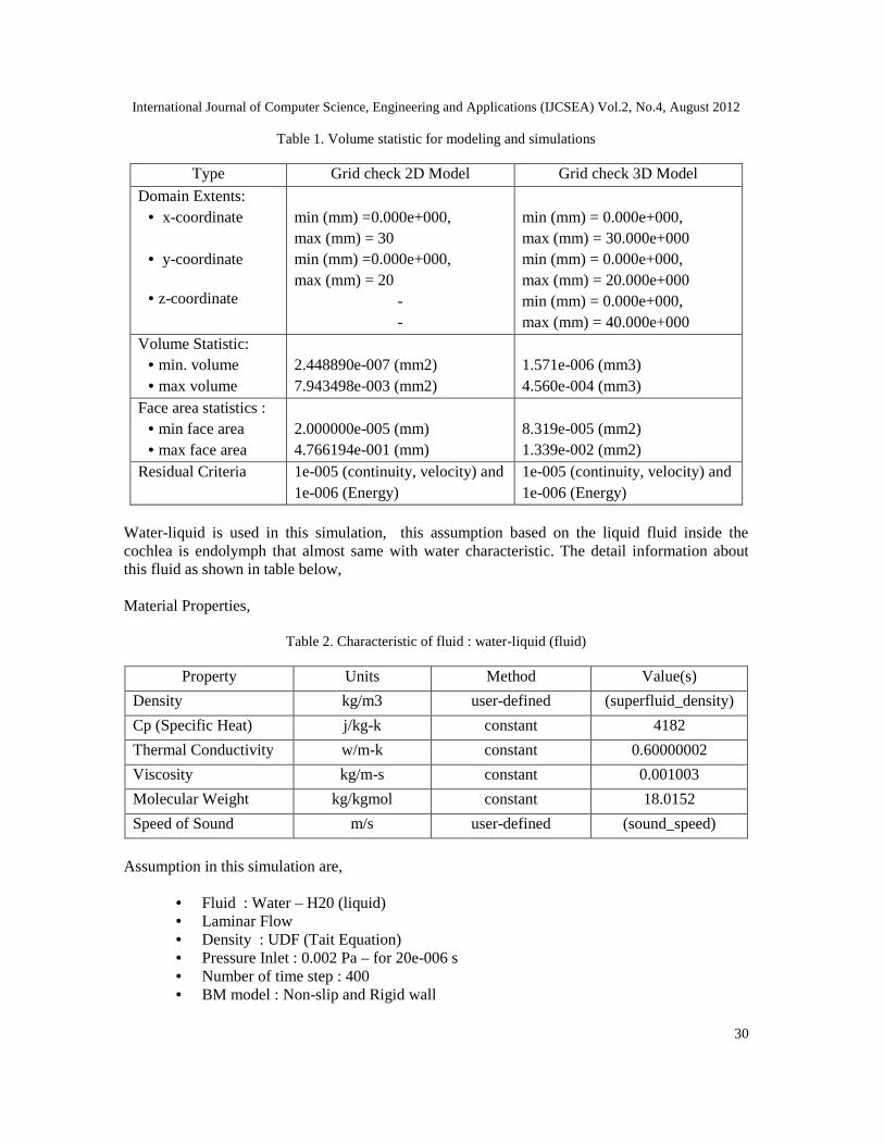
Table 1. Volume statistic for modeling and simulations
Type Grid check 2D Model Grid check 3D Model
Domain Extents:• x-coordinate
• y-coordinate
• z-coordinate
min (mm) =0.000e+000,max (mm) = 30min (mm) =0.000e+000,max (mm) = 20
--
min (mm) = 0.000e+000,max (mm) = 30.000e+000min (mm) = 0.000e+000,max (mm) = 20.000e+000min (mm) = 0.000e+000,max (mm) = 40.000e+000
Volume Statistic:• min. volume• max volume
2.448890e-007 (mm2)7.943498e-003 (mm2)
1.571e-006 (mm3)4.560e-004 (mm3)
Face area statistics :• min face area• max face area
2.000000e-005 (mm)4.766194e-001 (mm)
8.319e-005 (mm2)1.339e-002 (mm2)
Residual Criteria 1e-005 (continuity, velocity) and1e-006 (Energy)
1e-005 (continuity, velocity) and1e-006 (Energy)
Water-liquid is used in this simulation, this assumption based on the liquid fluid inside thecochlea is endolymph that almost same with water characteristic. The detail information aboutthis fluid as shown in table below,
Material Properties,
Table 2. Characteristic of fluid : water-liquid (fluid)
Property Units Method Value(s)
Density kg/m3 user-defined (superfluid_density)
Cp (Specific Heat) j/kg-k constant 4182
Thermal Conductivity w/m-k constant 0.60000002
Viscosity kg/m-s constant 0.001003
Molecular Weight kg/kgmol constant 18.0152
Speed of Sound m/s user-defined (sound_speed)
Assumption in this simulation are,
• Fluid : Water – H20 (liquid)• Laminar Flow• Density : UDF (Tait Equation)• Pressure Inlet : 0.002 Pa – for 20e-006 s• Number of time step : 400• BM model : Non-slip and Rigid wall
International Journal of Computer Science, Engineering and Applications (IJCSEA) Vol.2, No.4, August 2012
31
• Bulk Modulus (water) : 2.2E+09 Pa• Density water (at 1 atm) : 1000 kg/m3• Pressure Operating : 101325 Pa• Temperature Operating : 300 K
The criteria for convergence were 1.0×10⁻⁵ for continuity, velocity and energy. The time step sizeis determined to be 2.0 x 10⁻⁶ s and the total calculation time is 2.0 x 10⁻³ s.
• Input data :
• 10 time step with 0 Pa for 2.0 x 10⁻⁵ seconds• 10 following time step using 0.002 Pa for 2.0 x 10⁻⁵ seconds• 980 following time step using 0 Pa until 2.0 x 10⁻³ seconds
3. RESULTS AND DISCUSSION
In this paper, the liquid in the duct model is modeled as non-viscous fluid. The flow is a laminarflow model which was controlled by pressure on the pressure-inlet option. The simulation modelsare 2 and 3 dimensional square mesh with cartesian coordinate. The density of the cochlear fluidsthat was filled into the duct is estimated using UDF. The simulation process is carried out usingunsteady time dependent calculation.
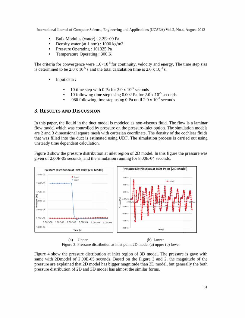
Figure 3 show the pressure distribution at inlet region of 2D model. In this figure the pressure wasgiven of 2.00E-05 seconds, and the simulation running for 8.00E-04 seconds.
(a) Upper (b) LowerFigure 3. Pressure distribution at inlet point 2D model (a) upper (b) lower
Figure 4 show the pressure distribution at inlet region of 3D model. The pressure is gave withsame with 2Dmodel of 2.00E-05 seconds. Based on the Figure 3 and 2, the magnitude of thepressure are explained that 2D model has bigger magnitude than 3D model, but generally the bothpressure distribution of 2D and 3D model has almost the similar forms.
International Journal of Computer Science, Engineering and Applications (IJCSEA) Vol.2, No.4, August 2012
31
• Bulk Modulus (water) : 2.2E+09 Pa• Density water (at 1 atm) : 1000 kg/m3• Pressure Operating : 101325 Pa• Temperature Operating : 300 K
The criteria for convergence were 1.0×10⁻⁵ for continuity, velocity and energy. The time step sizeis determined to be 2.0 x 10⁻⁶ s and the total calculation time is 2.0 x 10⁻³ s.
• Input data :
• 10 time step with 0 Pa for 2.0 x 10⁻⁵ seconds• 10 following time step using 0.002 Pa for 2.0 x 10⁻⁵ seconds• 980 following time step using 0 Pa until 2.0 x 10⁻³ seconds
3. RESULTS AND DISCUSSION
In this paper, the liquid in the duct model is modeled as non-viscous fluid. The flow is a laminarflow model which was controlled by pressure on the pressure-inlet option. The simulation modelsare 2 and 3 dimensional square mesh with cartesian coordinate. The density of the cochlear fluidsthat was filled into the duct is estimated using UDF. The simulation process is carried out usingunsteady time dependent calculation.
Figure 3 show the pressure distribution at inlet region of 2D model. In this figure the pressure wasgiven of 2.00E-05 seconds, and the simulation running for 8.00E-04 seconds.
(a) Upper (b) LowerFigure 3. Pressure distribution at inlet point 2D model (a) upper (b) lower
Figure 4 show the pressure distribution at inlet region of 3D model. The pressure is gave withsame with 2Dmodel of 2.00E-05 seconds. Based on the Figure 3 and 2, the magnitude of thepressure are explained that 2D model has bigger magnitude than 3D model, but generally the bothpressure distribution of 2D and 3D model has almost the similar forms.

International Journal of Computer Science, Engineering and Applications (IJCSEA) Vol.2, No.4, August 2012
32
(a) Upper (b) LowerFigure 4. Pressure distribution at inlet point 3D model (a) upper (b) lower
Figure 5 show the pressure distribution of 2D and 3D model at the center point of the membrane.In the figure, magnitude of the pressure distribution using 3D model has lower than 2D model.The wavelength of the 2D model is shorter than 3D model, so the frequency at the center point of2D model is higher than 3D model at the same conditions.
(a) 2D Model (b) 3D ModelFigure 5. Pressure distribution at distance 14.5 mm (a) 2D and (b) 3D model
Figure 6 show the pressure distribution of 2D and 3D model at the end point of 29 mm from basepoint. 2D model has more period than 3D, this indicate that analysis using 2D model has higherfrequency than 3D. It is caused by design of the model as dimension and amount of the griddifferent each other. The both graph of 2D and 3D showed to the periodical in oscillation with thevalue of the fluctuation that was not too big and the amplitude was tended to decreaseexponentially.
3D model2.5E-3
2.0E-3
1.5E-3
1.0E-3
5.0E-3
0.0E-3
-5.0E-3 Time (s)
0.0E0 1.0E-4 2.0E-4 3.0E-4 4.0E-4 5.0E-4 6.0E-4 7.0E-4 8.0E-4
International Journal of Computer Science, Engineering and Applications (IJCSEA) Vol.2, No.4, August 2012
33
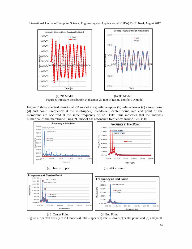
(a) 2D Model (b) 3D ModelFigure 6. Pressure distribution at distance 29 mm of (a) 2D and (b) 3D model
Figure 7 show spectral density of 2D model at (a) inlet – upper (b) inlet – lower (c) center point(d) end point. Frequency at the inlet-upper, inlet-lower, center point, and end point of themembrane are occurred at the same frequency of 12.6 kHz. This indicates that the analysisnumerical of the membrane using 2D model has resonance frequency around 12.6 kHz.
(a) Inlet - Upper (b) Inlet - Lower
(c ) Center Point (d) End PointFigure 7. Spectral density of 2D model (a) inlet – upper (b) inlet – lower (c) center point, and (d) end point
International Journal of Computer Science, Engineering and Applications (IJCSEA) Vol.2, No.4, August 2012
33
(a) 2D Model (b) 3D ModelFigure 6. Pressure distribution at distance 29 mm of (a) 2D and (b) 3D model
Figure 7 show spectral density of 2D model at (a) inlet – upper (b) inlet – lower (c) center point(d) end point. Frequency at the inlet-upper, inlet-lower, center point, and end point of themembrane are occurred at the same frequency of 12.6 kHz. This indicates that the analysisnumerical of the membrane using 2D model has resonance frequency around 12.6 kHz.
(a) Inlet - Upper (b) Inlet - Lower
(c ) Center Point (d) End PointFigure 7. Spectral density of 2D model (a) inlet – upper (b) inlet – lower (c) center point, and (d) end point
International Journal of Computer Science, Engineering and Applications (IJCSEA) Vol.2, No.4, August 2012
34
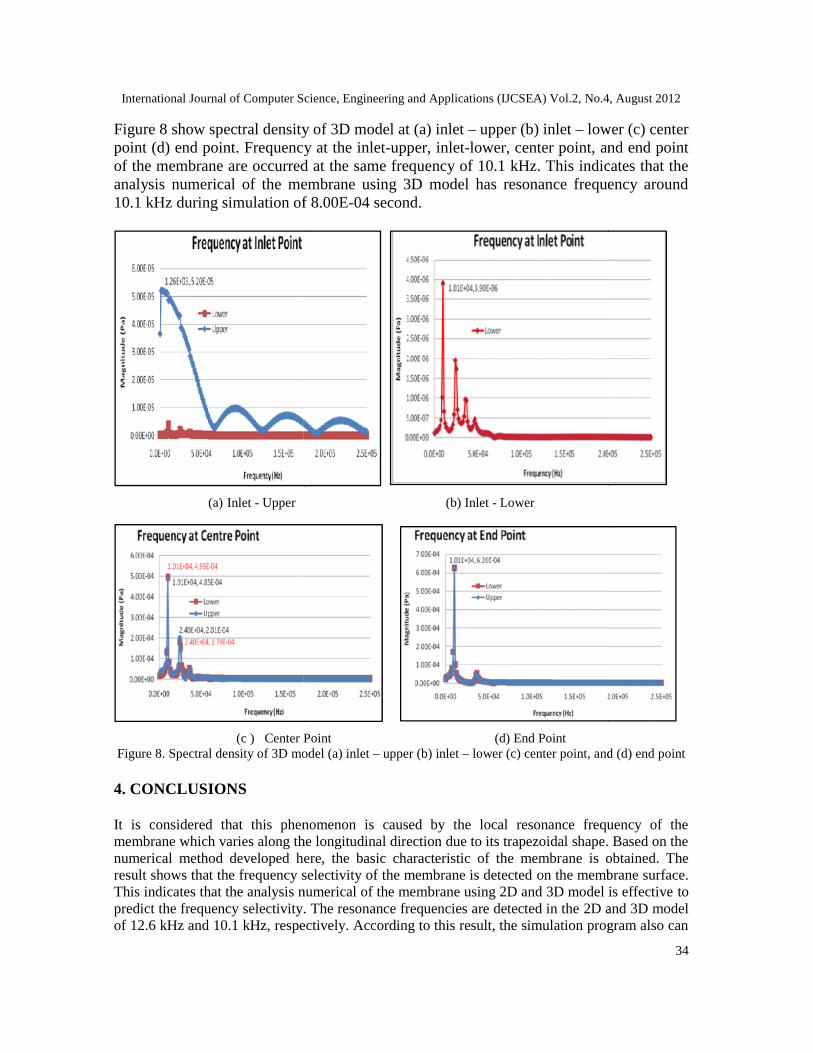
Figure 8 show spectral density of 3D model at (a) inlet – upper (b) inlet – lower (c) centerpoint (d) end point. Frequency at the inlet-upper, inlet-lower, center point, and end pointof the membrane are occurred at the same frequency of 10.1 kHz. This indicates that theanalysis numerical of the membrane using 3D model has resonance frequency around10.1 kHz during simulation of 8.00E-04 second.
(a) Inlet - Upper (b) Inlet - Lower
(c ) Center Point (d) End PointFigure 8. Spectral density of 3D model (a) inlet – upper (b) inlet – lower (c) center point, and (d) end point
4. CONCLUSIONS
It is considered that this phenomenon is caused by the local resonance frequency of themembrane which varies along the longitudinal direction due to its trapezoidal shape. Based on thenumerical method developed here, the basic characteristic of the membrane is obtained. Theresult shows that the frequency selectivity of the membrane is detected on the membrane surface.This indicates that the analysis numerical of the membrane using 2D and 3D model is effective topredict the frequency selectivity. The resonance frequencies are detected in the 2D and 3D modelof 12.6 kHz and 10.1 kHz, respectively. According to this result, the simulation program also can
International Journal of Computer Science, Engineering and Applications (IJCSEA) Vol.2, No.4, August 2012
34
Figure 8 show spectral density of 3D model at (a) inlet – upper (b) inlet – lower (c) centerpoint (d) end point. Frequency at the inlet-upper, inlet-lower, center point, and end pointof the membrane are occurred at the same frequency of 10.1 kHz. This indicates that theanalysis numerical of the membrane using 3D model has resonance frequency around10.1 kHz during simulation of 8.00E-04 second.
(a) Inlet - Upper (b) Inlet - Lower
(c ) Center Point (d) End PointFigure 8. Spectral density of 3D model (a) inlet – upper (b) inlet – lower (c) center point, and (d) end point
4. CONCLUSIONS
It is considered that this phenomenon is caused by the local resonance frequency of themembrane which varies along the longitudinal direction due to its trapezoidal shape. Based on thenumerical method developed here, the basic characteristic of the membrane is obtained. Theresult shows that the frequency selectivity of the membrane is detected on the membrane surface.This indicates that the analysis numerical of the membrane using 2D and 3D model is effective topredict the frequency selectivity. The resonance frequencies are detected in the 2D and 3D modelof 12.6 kHz and 10.1 kHz, respectively. According to this result, the simulation program also can
International Journal of Computer Science, Engineering and Applications (IJCSEA) Vol.2, No.4, August 2012
35
be applied to predict the pattern of pressure distribution and pressure changing on the membrane.This prediction can be used for the next step using experimental method.
ACKNOWLEDGEMENTS
The author would like to acknowledge Kawano Laboratory members at Osaka University Japanand the support of LPPI Tarumanagara University.
REFERENCES
[1] Békésy, von G., Current Status of Theories of Hearing, Science, 123 – 3201, 497 – 512, 1956.[2] Békésy, von G., Experiments in Hearing, Mc Graw Hill, New York, 1960.[3] Zwislocki, Josef J., Auditory sound trans-mission: an autobiographical perspective, Lawrence
Erlbaum Associates Inc., New Jersey, USA, 2002.[4] Moller, Aage R., Hearing, second edition : Anatomy, Physiology and disorders of the auditory
system, 2 nd edition, Elsevier, USA, 2006[5] Tu Jiyuan, Guan H. Yeoh, Chaogun Liu, Computational Fluid Dynamics : A Practical Approach, 1st
Edition, Elsevier, USA, 2008.[6] Versteeg H K and Malalasekera W, An Introduction to Computational Fluid Dynamics, second
Edition, British:Prentice Hall, 2007.[7] Batchelor G K, An Introduction to Fluid Dynamics, United States:Cambridge, 2007.[8] Ferziger Joel H., Peric, Milovan, Computational Methods for Fluid Dynamics, third rev. edition.
Germany:Springer, 2002.[9] Ward A.J. – Smith, Internal Fluid Flow- The Fluid Dynamics of Flow in Pipes and Ducts, Great
Britain:Pitman Press, 1980.[10] Fangyi Chen, Howard Cohen, Thomas G. Bifano, Jason Castle, Jeffrey Fortin, Christopher Kapusta,
David C. Mountain, Aleks Zosuls, and Allyn E. Hubbar, A hydromechanical biomimetic cochlea:Experiments and models, J. Acoust. Soc. Am. Volume 119, Issue 1, pp. 394-405, 2006.
[11] Liu Bo, Xiu L. Gao, Hong X. Yin, Shu Q. Luo, Jing Lu, A Detailed 3D Model of The Guinea PigCochlea, Brain Struct Funct (2007) 212:223-230, Springer-Verlag 2007.
[12] Tanaka, K., M. Abe, S. Ando, A novel mechanical cochlea "fishbone" with dual sensor/actuatorcharateristics, IEEE/ASME Transactions on Mechatronics 3 (2) 98–105, 1998.
[13] White R. D., K. Grosh, Microengineered hydromechanical cochlear model, Proceedings of theNational Academy of Sciences of the United States of America 102 (5), 1296–1301, 2005.
[14] Anderson J. David, Computational Fluid Dynamics, Mc Graw-Hill Science, 1995.[15] Steele, Charles R. and Taber, Larry A., Comparison of WKB Calculations and Experimental Results
for Three-Dimensional Cochlear Models, J. Acoustical Society of America, 65(4), April 1979.[16] Wittbrodt, M., S. Puria, and C.R. Steele, Developing a physical model of the human cochlea using
micro-fabrication methods, Audiology and Neurotology 11(2):104-112, 2006.
AuthorsHarto Tanujaya received S.T., M.T., and Ph.D. degrees in Mechanical Engineeringfrom Tarumanagara University (in 1996), University of Indonesia (in 1999) andOsaka University (in 2010), respectively. He is a lecturer and researcher atTarumanagara University and his fields of research are includes artificial cochlea,vibrations, and computational fluid dynamics (CFD). Recently, his currentresearch project is vibration of the artificial basilar membrane using specificmaterials.