international journal of coal geology -...
TRANSCRIPT
International Journal of Coal Geology 131 (2014) 90–105
Contents lists available at ScienceDirect
International Journal of Coal Geology
j ourna l homepage: www.e lsev ie r .com/ locate / i j coa lgeo
Imminence of peak in US coal production and overestimation of reserves
Nathan G.F. Reaver a, Sanjay V. Khare b,⁎a Department of Bioengineering, The University of Toledo, 2801 West Bancroft Street, Toledo, OH 43606, United Statesb Department of Physics and Astronomy, The University of Toledo, 2801 West Bancroft Street, Toledo, OH 43606, United States
⁎ Corresponding author at. 2801West Bancroft Street, TTel.: +1 419 530 2292.
E-mail address: [email protected] (S.V. Khare
http://dx.doi.org/10.1016/j.coal.2014.05.0130166-5162/© 2014 Elsevier B.V. All rights reserved.
a b s t r a c t
a r t i c l e i n f oArticle history:Received 13 February 2014Received in revised form 27 May 2014Accepted 27 May 2014Available online 6 June 2014
Keywords:Logistic modelCoal reserveCoal production forecastPeak coalUSA energyNon-linear fitting
Coal is the bulwark of US energy production making up about a third of all energy produced and about half of itselectricity generation capacity, over the last decade. Current energy policy in theUnites States assumes that thereis at least a century of coal remaining within the nation that can be produced at the current rate of consumption.This assumption is based on the large reported coal reserves and resources. We show that, in coal-producing re-gions and nations, historically reported reserves are generally overestimated by a substantial magnitude. Wedemonstrate that a similar situation currently exists with US reserves. We forecast future US coal production,in both raw tonnage and energy, using a multi-cyclic logistic model fit to historical production data. Robustnessof themodel is validated using production data from regionswithin theUS, aswell as outside, that have complet-ed a full production cycle. Results from themodel indicatemaximum raw tonnage coal productionwill occur in atime window between the years 2009 and 2023, with 2010 being the most likely year of such a maximum. Sim-ilarly, energy production from coal will reach a maximum in the years between 2003 and 2018, with 2006 beingthe most likely year of maximum occurrence. The estimated energy ultimate recoverable reserves (URR) fromthe logistic model is 2750 quadrillion BTU (2900 EJ) with 1070 quadrillion BTU (1130 EJ) yet to be mined,while the estimated raw tonnage URR is 124 billion short tons (112 Gt) with 52 billion short tons yet (47 Gt)to be mined. This latter value is merely a fifth of the long held estimate of 259 billion short tons (235 Gt).
© 2014 Elsevier B.V. All rights reserved.
1. Introduction
1.1. Coal, carbon dioxide, and climate
Coal is a prominent non-renewable fuel composed mostly of carbonand hydrocarbons (EIA, 2013b). Coal has been an increasingly impor-tant energy source for the United States and the world since the indus-trial revolution (Höök et al., 2012). Of themajor fossil fuels, coal, oil, andnatural gas, it is coal that is the most carbon intensive (Moomaw et al.,2011). Due to its long-term use and high carbon intensity, coal has in-troduced a large amount of carbon dioxide to the atmosphere. The ef-fects of atmospheric carbon dioxide on the Earth's climate as agreenhouse gas and its connection with the burning of coal are wellknown. The Intergovernmental Panel on Climate Change (IPCC) hasstated it is very likely that most of the observed increase in global aver-age temperature since the mid-20th century is due to anthropogenicgreenhouse gas concentrations (Arrhenius, 1896; IPCC, 2007). TheIPCC forecasts several scenarios for coal and other fossil fuel productionprofiles as inputs for their climate models (IPCC, 2000, 2007). Forecast-ing relies on accurate estimates of remaining coal reserves as well as
oledo, OH 43606, United States.
).
reasonable estimates of the shape of the future production profile toknowhow those reserveswill be consumed over time. Current IPCC sce-narios have been criticized for using unrealistic production profiles(Höök and Tang, 2013; Patzek and Croft, 2010; Rutledge, 2011a). Thecritical role of coal is understood by noting that approximately 164 bil-lion metric tons or 44% of all historical carbon dioxide emissions fromthe US fossil fuel consumption came from US coal (EIA, 2011b, 2012d,2013a). The US has the largest reported coal reserves of any nation, con-taining approximately 28% of the world's reported reserves (BP, 2010),though it is possible that this percentage is inflated from the inaccuratereporting of China's reserves (Wang et al., 2013). If the US reservesare accurate, their extraction and combustion would amount to anaddition of 544 billion metric tons of carbon dioxide to the atmosphere(EIA, 2011b, 2012f, 2013a), which would be about 45 times 2013global emissions! Over the past 10 years the US has on average emitted2.077 billion metric tons of carbon dioxide per year from the use ofcoal, which is approximately 17% of the average total global emissions(EIA, 2014a). Emissions from US coal consumption have historicallymadeup a sizable portion of overall global emissions, and canbe expect-ed to have significant contribution in the future. It is therefore animperative to forecast future US coal production accurately. This isnot only necessary for the purpose of accurate climate modeling,but also needed because coal is fundamental to the world's current ful-filment of electrical energy demand and industrial processes.

91N.G.F. Reaver, S.V. Khare / International Journal of Coal Geology 131 (2014) 90–105
1.2. Coal in the USA
Coal has on average provided 31% of all US energy consumption and48% of electricity production over the past 10 years (EIA, 2012b, e). Thismakes coal the largest source of electricity in the US. Electricity is vitaltomodern day civilization in the US, as it has been integrated into almostevery aspect ofmodern life. From lighting and refrigeration towater treat-ment and health care, without electricity our society cannot function. Inaddition to being the largest source of electricity, coal also produces themost inexpensive electricity of all the fossil fuels (EIA, 2013c). Giventhat almost half of US electricity is produced from coal, any unforeseendecreases in the coal supply to electric utilities will have significant eco-nomic and social consequences. In addition to being an important energysource for electricity generation, coal is utilized as a rawmaterial in indus-trial applications. Approximately 5% of the US coal produced is used foractivities other than power generation (EIA, 2014b). The largest and per-haps most important use of coal as a rawmaterial is in the production ofiron and steel. Iron and steel are the most widely used metals in the USand theworld, comprising 95% of all tonnage of metal produced annually(USGS, 2014a). Iron and its alloys are integral parts to almost all indus-tries. Iron production from iron ore requires large quantities of coke,which is derived from coal (WCA, 2014). In the US, approximately 40%of steel is produced in blast furnaces, requiring coal-derived coke, withthe remaining 60% produced from recycled steel in electric arc furnaces(AISI, 2014). The importance of coal to iron and steel production is evenlarger on the global scale, with 70% of the world's production requiringcoke (WCA, 2014). A decrease in the supply of metallurgical coal formetal production would have as large of an impact to society and theeconomy as would a decrease in electrical production from coal.
1.3. Aims and scope of study
In this study, we performed a detailed analysis of the status of US coalproduction and forecasted future production using a multi-cyclic logisticmodel. The model was fit only to historical coal production data. Thishas an advantage over one-cycle logistic models that are fit to reservesas well as historical production data, because the fits are not restrictedby potentially biased or inaccurate reserve data, which can skew results.We emphasize our approach uses only historical production data whichare reliable, while excluding any consideration of unreliable reservesdata. Others have noted the unreliability of reserves (Glustrom, 2009;Höök and Aleklett, 2009, 2010; Rutledge, 2011a; Zittel and Schindler,2007) and have used modeling and forecasting techniques that do notrely on them (Patzek and Croft, 2010; Rutledge, 2011a). The validity ofthemulti-cyclic logistic model fits was rigorously tested using productiondata from several regions that have completed a full production cycle.Using these same regions, we also explored the historical accuracy of re-ported reserves and discovered a general pattern of gross overestimationof reserves. Our tests indicate that the multi-cyclic logistic model is morerobust in predicting future coal production profiles than extrapolatingproduction from reported reserves. In addition the model produces com-parable results to previous studies of US coal production. See Sections 3.2,Sensitivity Tests for Year of Peak Production and 3.6, Comparison to Pre-vious Results. Our results reveal that US coal production will peak in thenear term i.e. within a decade at the latest. The total US reserves are esti-mated to be a fifth of generally quoted estimates of over 200 years of sup-ply at current production levels. Both predictions have profoundimplications for the future scale of (i) climate change potential and (ii) in-dustrial activity of the US and the world.
2. Methods
2.1. Forecasting and prior work
Forecasting future coal production and the lifetime of reserveshas been of interest both historically and of late, due to coal's
importance to society, the economy, and more recently, climatechange. Some of the earliest work on the forecasting of coal produc-tion, with emphasis on the United Kingdom, can be credited toWilliams Stanley Jevons in 1865 (Jevons, 1865). Early forecasts ofUS coal production were completed by United States GeologicalSurvey scientists Campbell, Parker, and Garnett between 1908 and1917. Garnett predicted that all of the easily accessible coal in theUS would be exhausted by 2040, and all coal exhausted by 2050(USGS, 1909). Similar conclusions were reached by Campbell andParker (Campbell, 1917; USGS, 1909). The understanding of the na-ture and shape of minable energy resource (i.e. coal) productionprofiles was advanced by M.K. Hubbert in the 1950s (Hubbert,1949, 1956, 1969, 1976) whose work provides the basis for the con-cept of “peak coal,” where production reaches a maximum and be-gins a terminal decline on average. The general form of theproduction profile is bell shaped, though it is not always symmetric(Bardi, 2005). Recently, there have been several studies and com-mentaries on forecasting world coal production that utilize the con-cept of peak coal, including: Zittel and Schindler (2007), S. Mohr andEvans (2009), Patzek and Croft (2010), Heinberg and Fridley (2010),Höök et al. (2010), and Rutledge (2011a). These studies have usedvarious techniques to predict possible production scenarios whichinclude: logistic production growth fitted to estimated remainingreserves (Höök et al., 2010; Zittel and Schindler, 2007), an individualmine production level model incorporating supply and demand(S. Mohr and Evans, 2009), multi-Hubbert cycle fitting to historicalproduction data (Patzek and Croft, 2010), and logit and probittransform fits to historical production data (Rutledge, 2011a). Theresults of all of these different methods have been remarkably sim-ilar in that they all suggest that there is significantly less coal avail-able to the world than reported reserves and resources wouldindicate.
There have also been studies that focus only on forecastingproduction of individual countries with significant production,namely China and the US. Forecasting of future Chinese coal produc-tion has been done by Tao and Li (2007) and Lin and Liu (2010). Bothstudies resulted in similar predicted peak years for Chinese produc-tion between the late 2020s and early 2030s. Studies specificallyrelated to US production have been done by Glustrom (2009) andHöök and Aleklett (2009, 2010). Glustrom completed a detailedmine-level analysis of the Powder River Basin, in Wyoming. Höökand Aleklett divided the US into three coal-producing regions andused Hubbert linearization and logistic and Gompertz curve fits tohistorical production data, as well as, reported reserves, to forecastthe ultimate recoverable reserves and the timing of peak production.They concluded that the US would likely reach peak production by2030 unless significant development of reserves in the state ofMontana occurred. Based on their analysis the current US reportedreserves will likely not be completely realized in the future, andhence likely overstated.
2.2. Model description
Amethod for predicting the production profile of a finite extractableenergy source, such as coal is the multi-cyclic logistic model (Al-Fattahand Startzman, 1999, 2000; Nashawi et al., 2010; Patzek and Croft,2010). Its single cycle version is historically well known in mining(Bardi, 2005; Hubbert, 1949, 1956, 1969, 1976), as well as, in otherareas such as population dynamics and ecology (Lotka, 1910; Verhulst,1845).We describe here its basic assumptions and resulting productionprofile and apply it to data of US coal production in the Results section.In the next Section, 2.3, we discuss limitations and considerations thatmust be taken into account when using the multi-cyclic logisticmodel. Let A(t) be the cumulative quantity of coal mined at time t. LetB(t) be the quantity of coal remaining below ground at time t. Thebasic assumptions of the logistic model, for non-renewable energy
92 N.G.F. Reaver, S.V. Khare / International Journal of Coal Geology 131 (2014) 90–105
extraction,may be expressedmathematically by two simple state equa-tions of a first-order nonlinear system:
A tð Þ ¼ − B tð Þand A tð Þ ¼ kA tð ÞB tð Þ; ð1Þ
where k is a constant. A dot over a symbol denotes differentiation withtime. The first of these is an equation of continuity. It signifies the as-sumption that the quantity of coal mined adds to the above groundquantity, A(t), while simultaneously subtracting an equal quantityfrom the coal below ground, B(t). The second equation states that therate of coal extracted is linearly proportional to two types of quantities:the amount of coal below ground, B(t), and the quantity alreadymined,A(t). Of these, the first proportionality is easy to understand as themin-ing activity is proportional to the reserve base, B(t), available. The sec-ond is more subtle. It represents a monotonic relationship betweenthe quest for energy sources and the scale of the economy. The scaleof the economy in turn depends on the historicallymined energy sourcealready in existence, A(t). Thus, the rate of production of coal, A tð Þ, be-comes proportional to the cumulative production, A(t). Now, the sys-tem in Eq. (1) may be analytically solved to obtain,
A tð Þ ¼ 2σq 1þ tanht−τ2σ
� �� �; giving A tð Þ ¼ qsech2 t−τð Þ
2σ
� �;
where q≡ A t0ð Þ þ B t0ð Þ4σ
;
τ ≡ t0 þ σ lnB t0ð ÞA t0ð Þ
� �; and σ ≡ k A t0ð Þ þ B t0ð Þð Þ½ �−1
ð2Þ
The time, t0, is the initial time, the initial energy input tomine coal isA(t0), which is also related to the size of the economywhen society be-gins mining coal, and finally, the minable coal reserves are B(t0). Thecurve for A tð Þ vs. t from the system in Eq. (2) is a bell-shaped curve,which rises exponentially in the beginning, flattens and then decays.Thus it displays a peak, or maximum, in production. This model can befit to historical coal data of individual mining regions in the US andother coal-producing regions throughout the world. The agreement ofthe fitted equation to the general bell shape of the raw productiondata gives credibility to the assumptions in Eq. (1).
For analyzing large spatially separated coal basins a logistical analy-sis based on Eqs. (1) and (2) needs to be carried out for each individualregion and the production profiles summed. This model is called themulti-cyclic model. Such a model is appropriate where the extractionof coal in disparate regions becomes decoupled and individual coal ba-sins act within their own individual logistic model. Parts of the USwere mined serially, instead of simultaneously. Such a model is neces-sary to analyze their production profiles. It is also applicable where pro-duction in a single basin is undertaken sequentially in differentmines asopposed to being pursued concurrently in every sub-section. Each ofthese sub-sections then undergoes a separate, generally, bell-shapedcurve for its production. As pointed out by (Bardi, 2005), the curve isnot necessarily symmetric. Themulti-cyclic logistic model is also appro-priate when social or political events change the relationship (i.e.change in the k constant in Eq. (1)) between the quest for energysources and the scale of the economy, resulting in the start of a newcycle. The model may be described by the following set of equations:
A tð Þ ¼Xni¼1
Qi tð Þ; where Qi tð Þ ¼ 2σ iqi 1þ tanht−τi2σ i
� �� �;
yielding; A tð Þ ¼Xni¼1
qi sech2 t−τið Þ
2σ i
� �:
ð3Þ
Here τi, σi, qi are fitting parameters having an interpretation similarto their corresponding analogues in Eq. (2) for each individual miningregion i. The total number of maxima in these curves is n and hence de-notes the total number of coal basins that were mined sequentially in agiven region. These equations give the cumulative quantity of coal A(t)
and the instantaneous production, A tð Þ, which shows the growth anddecline of coal production. The value A(∞) provides an estimate of thetotal coal that may be mined, or ultimate recoverable reserves (URR).In this study the URR is a fitting parameter that is thus derived fromhis-torical production data, A tð Þ, and not taken from reported reserves fromhistorical databases. It can be obtained by,
URR ¼Z ∞
−∞A tð Þdt ¼
Xni¼1
4σ iqi: ð4Þ
Wehave applied the solutions in Eq. (3) to historical coal productiondata from five geographical regions within the US and consequently tothe entire US. Our analysis provides an estimate, by region as well asfor the entireUS, of thequantities of: (i) ultimate cumulative production(A(∞)), (ii) maximumyearly production of total raw coal and the year itoccurs, and (iii) the rank and quality of coal. Combining (ii) and (iii) andusing a heat energy value associated with each rank of coal we obtain(iv) the quantity of maximum yearly heat energy production fromcoal and the year it occurs. To test the sensitivity of our analysis to ourmodeling approach we have analyzed production profiles of 12 com-pleted coal production cycles. A mining cycle can be defined as the ini-tiation and increase of production to the reaching of its maximum andits subsequent decline and end. Of these 12 cycles, two typical examplesare presented. The first cycle is for a single country, theUnited Kingdom.Here the cycle of mining coal is nearly complete. The other cycle is forthe mining of anthracite coal in the US state of Pennsylvania.
The ultimate recoverable reserves (URR) are defined as the totalamount of coal that can be mined from a specific geographic area. Thisupper limit can be reached due to a variety of factors. For example, allof the coal in the region could be mined to exhaustion, or the coalthat remains in the ground is too expensive, either monetarily orenergetically, to be extracted. The URR is generally estimated by the re-ported coal reserves for a region combined with the cumulative (total)amount of coal that has already been mined from that region. Reportedreserves can change over time for a variety of reasons. Reserves can bedepleted, new reserves can be found, reserves could have been over-or underestimated in the past and be updated, or changes in energyand environmental policy can affect reported reserves (Höök andAleklett, 2010). Estimates obtained from fitting production profiles tosmooth fits to Eq. (3) often differ from reported reserves. To quantifythis over- or underestimation of reserves frompredictions of the logisticmodel, we define a quantity called “estimated error in URR” δURR%(t) attime t. It is defined by the equation:
δURR% tð Þ ¼ ΔURRURR
100%ð Þ ¼ C tð Þ þ R tð Þ−URR½ �URR
100%ð Þ
¼ EUR tð Þ−URR½ �URR
100%ð Þ:
ð5Þ
Here C(t) is the cumulative production of coal as of year t computedfrom past reported production figures, R(t) are the reported reserves atyear t, EUR(t) is the estimated ultimate recovery and is the sum of R(t)and C(t), and URR is the total coal mined when reserves have reachedzero theoretically and production has ceased. The URR is obtained byfitting Eq. (3) to the production data so that URR ≡ A(∞). We note thedifference of our approach to compute URR from other methods (Höökand Aleklett, 2009, 2010; Zittel and Schindler, 2007), where URR is ob-tained from different independent methods of reserves determination.For regions where the mining cycle has neared completion (e.g. theUnited Kingdom, France, Japan, and anthracite coal in Pennsylvania), itis possible to determine if reported coal reserves in that regionwere his-torically over- or underestimated since the URR can be calculated direct-ly from the historical production data rather than be generated from afit of Eq. (3). If δURR%(t) N 0 it implies that the reported reserves R(t)are higher than the theoretical expectation from Eq. (3). Likewise, ifδURR%(t) b 0 it implies that R(t) are lower. If the reported reservesmatch the theoretical estimate then δURR%(t) is precisely zero.
1 One short ton = 2000 pounds.2 It should be noted that since 2008 US coal production has been in steep andmonoton-
ic yearly decline, potentially making 2008 the year of peak production. US coal productionin 2013 has dropped below 1 billion short tons for the first time since 1993.
3 It is a historical observation in the state by state, EIA database that energy content ofcoal on average remains relatively constant or decreases slightly over time for a givenstate. This may not be a general phenomena but it appears to be the case here. With thisobservation we can take a conservative approach and safely assume that using the energycontent value from1960 in earlier years to 1800may slightly underestimate the actual en-ergy produced in these years, i.e. 1800–1959. The EIA appears to have used this method intheir database as well. In their database all reported coal energy content values from eachstate for the years 1960–1972 are constant values.
93N.G.F. Reaver, S.V. Khare / International Journal of Coal Geology 131 (2014) 90–105
2.3. Considerations in the use of the multi-cyclic logistic model
The multi-cyclic logistic model has been used to describe and fore-cast the production profiles of a variety of non-renewable extractableenergy sources such as oil, natural gas, and coal (Al-Fattah andStartzman, 1999, 2000; Nashawi et al., 2010; Patzek and Croft, 2010).As with the application of any theoretical model it is important to beaware of its limitations. As was stated previously, themulti-cyclic logis-tic model is appropriate to use when historical data do not follow a sin-gle logistic cycle. Deviations of a production profile from the theoreticalsingle cycle can be due to a variety of reasons (e.g. economicallydecoupled coal regions, wars, depressions, regulations, etc.) It is evidentfrom thehistorical production data that these disruptionshave occurredin the past and can be expected to happen in the future. Themulti-cycliclogisticmodel can only attempt to forecast the future production profileof the last incomplete cycle. For example, US coal production has gonethrough two productions maximums in the past and is currently in athird cycle. The multi-cyclic logistic model assumes that the third in-complete cycle is the final one in the production profile. There couldbe future disruptions in production due to a variety of factors, butpredicting these fluctuations would require clairvoyance. The modelprovides the overall trends in future production given that there arenot significant disruptions to production. Each cycle of the multi-cycliclogistic model is independent of the others, so the production data areessentially segmented, reducing the importance of long-term trendspresent from earlier cycles in decline. This can be thought of as adouble-edged sword. The reduction of long-term trends can potentiallycause themulti-cyclic logistic model to forecast earlier peaks in produc-tion and smaller URRs than single cycle methods. However, this reduc-tion in values of the year of peak production and predicted URR isprecisely the point of the multi-cyclic logistic model. It is a change tothe predictions of single cycle models that goes in the correct direction.It partially decouples the most recent incomplete cycle from previousproduction disruptions and trends that could skew results of a singlecycle analysis. Still, themulti-cyclic logistic model is a curve fitting tech-nique at its core, and one should be cautious in its use to ensure it pro-duces meaningful results.
Themulti-cyclic logistic model has 3n free parameters, where n rep-resents the number of cycles. In principle it is possible to improve the fitof the multi-cyclic logistic model to historical coal production data byincreasing the number of cycles, and hence the number of free parame-ters. This can result in statistical over-fitting of the model to the data.Therefore, the “goodness of fit” of the model to the data is not a com-plete measure of the model's quality. A statistical likelihood ratio testbetween multi-cyclic logistic models with differing numbers of cyclesfitted to the same data can be used to justify the number of cyclesused (Anderson and Conder, 2011). We discuss this in depth inSection 2.5 Logistic Model Fitting. Another issue of the multi-cyclic lo-gistic model is that it can potentially have a large number of free param-eters. Increasing the number of free parameters can reduce the accuracyof the forecast. However, each of the parameters has a well-definedphysical meaning that can be easily estimated for complete cyclesfrom a chart of historical data. This allows for the parameters of early cy-cles to be determined with a high degree of accuracy. The fitting proce-dure is effectively reduced to the last incomplete production cycle. It isalways advisable to use only the minimum number of cycles neededto describe the data to prevent over-fitting of the model.
Anderson and Conder provide a detailed discussion and critique ofthe use of the model in forecasting future petroleum production(Anderson and Conder, 2011). Their discussions can also be applied toother non-renewable extractable energy resources, such as coal. Themain aim of this study is not necessarily to forecast future US coal pro-duction with a very high degree of accuracy of single digit percentagelevel, but rather to study US coal production from a variety of perspec-tives to draw overall conclusions of future production. The multi-cycliclogistic model is definitely useful as one of these perspectives.
2.4. Data sources
Historical production data for the major coal-producing regions inthe United States were obtained from the United States Geological Sur-vey (USGS) COALPROD Database (Milici, 1997) for the years 1800–1995. Data from the USGS consisted of yearly production quantities ofcoal, in units of short tons,1 for all coal-producing states in the USwhich are divided into five regions: (i) Appalachian, (ii) Illinois Basin,(iii) Gulf Coast, (iv) Great Plains, and (v) Western coal-producing re-gions. The Appalachian region is comprised of the states Alabama,Georgia, Kentucky, Maryland, Ohio, Pennsylvania, Tennessee, Virginia,and West Virginia. The Illinois Basin region consists of Illinois andIndiana. The Gulf Coast region consists of Louisiana and Texas. TheGreat Plains region consists of North Dakota and South Dakota. TheWestern region is comprised of Arizona, Colorado, Montana, NewMexico, Utah, and Wyoming. A second source of data was the UnitedStates Information Administration (EIA) coal production database(EIA, 2011a) for the years 1960–2008. Data after 2008 were omittedto provide a more conservative fitting procedure. The worldwide eco-nomic crisis starting in 2008 and the increase in production of naturalgas from hydraulic fracturing in the US have reduced demand for coal.This declinewould bias the fitting procedure to predict earlier peak pro-duction years and lower URRs. The omission allows for thefitting resultsto give more conservative forecasts of US coal production as it wouldhave likely proceeded based on the previous trend without these twoconfounding components.2 The USGS production data from 1800 to1995 were combined with production data from the EIA database, foreach state, for the years 1996–2008. In the overlapping years 1960–1995 both datasets agreed with each other with a maximum error of3.3%. In these overlapping years the USGS production data were used.Thus a historical dataset, from 1800 to 2008, of yearly production ofcoal in million short tons was generated from the combined USGS andEIA databases. There were several states with some coal production in-cluded in the EIA database thatwere excluded from theUSGS long-termdatabase, namely Alaska, Arkansas, Kansas, Mississippi, Missouri, andOklahoma. However, all of these states were observed to be in a postpeak declining production phase and had negligible production, onlymaking up 0.5% of US production, and hence were omitted from theanalysis. The EIA database further provided average energy content ofcoal produced in each state per year, in units of million British ThermalUnits (BTU) per short ton, for all its years. This energy content factor,converting raw tons of coal to BTU of energy, was multiplied by eachstate's production for years 1960–2008. For years 1800–1959, the aver-age energy content for coal produced in 1960was used.3 The yearly pro-duction and yearly gross energy production of coal for each of the fiveregions were then added to produce a yearly quantity of productionfor (i) raw coal and (ii) gross energy for the entire United States. Datafrom the National Coal Resource Data Systems (NCRDS) State Coopera-tives Project (USGS, 2014b) list the rank of coal reserves in each state aseither anthracite, bituminous, sub-bituminous, or lignite. Each coal rankhas an energy content associated with it measured in units of millionBTUper short ton. The energy content of each rank of coal has a relative-ly wide range, so it is not possible to determine the explicit energy con-tent from only the rank information. The energy content ranges of coal
94 N.G.F. Reaver, S.V. Khare / International Journal of Coal Geology 131 (2014) 90–105
within each rank vary enough that there can be overlap of these rangesbetween the various ranks. Anthracite and bituminous coals lie in an en-ergy range of 24–32with themajority of the supply of the former occu-pyinghigher values andmajority of the supply of the latter having lowervalues within these bounds. Sub-bituminous and lignite coals have en-ergy values in the ranges of 16.6–24 and 10–16.6, respectively(Schweinfurth, 2009). Coal rank from each state was classified as eitheranthracite, bituminous, sub-bituminous, or lignite using this database.The rank assigned was checked to be consistent with energy contentfactor provided in the EIA database by confirming that it lays in therange given for each rank above (Schweinfurth, 2009; USGS, 2014b). Ayearly production dataset was created for Pennsylvania anthracite coalproduction using the same datasets and procedure as used for the re-gional and US datasets. A yearly production dataset for the UnitedKingdom (UK) was created from yearly production data in BritishHistorical Statistics (Mitchell, 1988), in units of million short tons andcovering years 1830–1980. This dataset was combined with UK coalproduction data from 1981 to 2008 from the BP statistical review (BP,2010). Consistency of values between the two datasets was checkedbetween the years 1980 and 1981, with the values differing by lessthan 2%.
Historical coal reserve data for the US, UK, and Pennsylvania anthra-cite coal were obtained from the supplemental material in Rutledge(2011a, b). Historical production data for the additional sensitivitytests performed on Belgium, France, Japan, the Netherlands, Portugal,South Korea, Sweden, Taiwan, and the US states of Georgia and SouthDakota, as described in Section 2.6, were obtained from EIA (2011a),Milici (1997), and S.H. Mohr and Evans (2009). Historical coal reservedata for these additional tests were obtained from Rutledge (2011b).
2.5. Logistic model fitting
Themulti-cyclic logistic model, as given in Eq. (3), was fit to the var-ious datasets using a nonlinear regression technique, described in thissection. The function chosen for optimization for this study was thesum of the squares of the error (SSE) between the multi-cyclic logisticmodel and historical production data,
SSE qif g; τif g; σ if gð Þ ¼Xmj¼1
Q t j� �
−Af t j; qif g; τif g; σ if g� �h i2
: ð6Þ
The historical production data are given in the form, t j; Q t j� �� �
,where Q t j
� �is the coal production in the year tj. The total number of
data points available for the fit is m. A trial fit to this dataset withEq. (3) is A f t j; qif g; τif g; σ if g� �
. Thus SSE is only a function of the fittingparameters in Eq. (3). The values of these parameters which minimizethe SSE, and are physically possible (i.e. non-negative), produce thebest fit of the multi-cyclic logistic model to the historical productiondata. The best fit was determined by computationally finding the mini-mum of the SSE function. This process consisted of assigning initialvalues to the fitting parameters, {τi, σi, qi}, and iteratively changingthe parameter values in the direction of the negative gradient of theSSE function until the gradient was effectively zero, −∇!SSE ¼ 0. It ispossible that the SSE function can have multiple minima. The initialvalues of the fitting parameters were carefully chosen so that the opti-mization algorithmwould find the lowest minimum. The number of cy-cles, n, in the model, from Eq. (3), along with the an initial trial set offitting parameters, τi, σi, and qi, were determined by visual inspectionof the historical production data. From the nature of Eq. (3) it is clearthat τi are the time values at which maxima or peaks occur for the pro-duction in each cycle, The values for qi are related to the productionrates at the maxima or peak of production, while σi are the measure ofthe width or sharpness of the curves.
As stated previously in Section 2.3, the “goodness of fit” or SSE of themodel to the data is not a complete measure of the model's quality. A
statistical likelihood ratio test between multi-cyclic logistic modelswith differing numbers of cycles fitted to the same data was used to jus-tify the number of cycles used in each fitting procedure. The likelihoodratio test demonstrates whether or not the decrease in the SSE of thefit is improved more than would be expected by simply adding moremodel parameters (Anderson and Conder, 2011). The likelihood ratiotest utilizes the F-test. The F-statistic for the likelihood ratio test is de-scribed as,
F ¼ SSE1−SEE2ð Þ= 3n2−3n1ð ÞSSE2= m−3n2−1ð Þ ; ð7Þ
where SSE1 (or SSE2) is the minimum SSE of the fit frommodel with n1(or n2) number of cycles, where n2 N n1, and m is the total number ofdata points used in the fitting. The degrees of freedom for this testare 3(n1 − n2) and (m − 3n2 − 1). The p-value obtained fromthis test gives the probability that the improved fit (i.e. smaller SSE) ofthe model to the production data, from the addition of an additionalcycle, is due to the increase of the number of free parameters, ratherthan the model describing the data better. p-Values less than 0.05 aregenerally considered significant, corresponding to a confidence levelof 95%.
In all a total of seven best fits were computed: one each for theraw tonnage and gross energy content coal production of the entireUS and for the raw tonnage coal production of the five coal-producingregions. The logistic models used in these fits consisted of either twoor three cycles. For each of the seven best fits we tested for over-fitting using the likelihood ratio test. Each of the seven fits were com-pared using the likelihood ratio test to the best fit of a one-cycle, two-cycle, three-cycle, and four-cycle model to the historical data of thatcoal region. All of the tests gave a confidence level of over 99% thatmodel did not suffer from statistical over-fitting.
In addition to the best fits, lesser quality fits (i.e. with SSEs largerthan the best fit) were found with peak years preceding and followingthe peak year of the last cycle of the best fit model for each of theseseven datasets. These fits were found by biasing the initial values ofthe parameters, τfinal, σfinal, and qfinal, for the last, incomplete cycle inthe model, so that the optimization algorithm could fall into a nearbylocal minimum. The lesser quality fits were restricted to having SSEsno larger than 10% of the SSE of the best fit.
2.6. Sensitivity tests
The sensitivity of the fitting procedure to how far a productionprofile has advanced was tested using data for 12 very different butnear complete coal production profiles, namely Belgium (URR of2611 Mt), France (URR of 4579 Mt), Japan (URR of 2944 Mt), theNetherlands (URR of 585 Mt), Portugal (URR of 27 Mt), South Korea(URR of 589 Mt), Sweden (URR of 29 Mt), Taiwan (URR of 181 Mt),the United Kingdom (URR of 26470 Mt), and the US states ofGeorgia (URR of 11 Mt) and South Dakota (URR of 1 Mt). Productionfor only anthracite coal from Pennsylvania (URR of 5053 Mt) was alsoanalyzed. In this article we highlight two typical cases among these12: (i) the total coal production of the United Kingdom and (ii)only the production for anthracite coal from Pennsylvania. In additionto the highlighted UK and Pennsylvania anthracite, we include threefigures of our analysis for France, Japan, and Sweden in Appendix A.These regions' historical peak in production occurred later in the pro-duction cycle due to the asymmetry of production profile. However,the logistic model still provides reasonable forecasting of their pro-duction profiles. Our validation uses single cycle logistic models fitto truncated historical production data. For this purpose we startedby first fitting a logistic model to the entire dataset and obtainingthe peak production value for this best fit. Truncated datasets are cre-ated by taking data from the start of production up to the productionlevel corresponding to approximately 25%, 50%, 75%, and 100% of the

Table 1Parameters of best fit three-cycle logistic models, of Eq. (3), for US coal raw tonnage pro-duction (left two columns) and US coal energy production (right two columns) shown inFigs. 1 and 2. Also given are p-values for likelihood ratio tests for over-fitting between bestfit multi-cyclic logisticmodels containing between one and three cycles. p-Values give theprobability that the improved fit to the data of a logistic model with more cycles over onewith less cycles is due to over-fitting. 1 minus the p-value gives the probability that the
95N.G.F. Reaver, S.V. Khare / International Journal of Coal Geology 131 (2014) 90–105
best fit peak production value. Best fit curves were generated usingonly the truncated datasets. This process illustrates the accuracy ofthe logistic model's forecasts as the actual production proceedsthrough time. These fits were compared with the best fit modelfrom the entire dataset.
2.7. Reserves vs. model
We computed the δURR%(t) for 10 regions, namely, Belgium, France,Japan, the Netherlands, Portugal, Sweden, Taiwan, UK, Pennsylvania an-thracite, andUS.Wewere restricted to these 10 regions as they had bothlong-term historical production data and long-term historical reservedata. We highlight the (i) UK and (ii) Pennsylvania anthracite regionsas typical cases, and analyze the (iii) US. For the entire US the estimatedδURR%(t) was generated using the best fit model to calculate the URR asgiven in Eq. (5), while for the UK and Pennsylvania anthracite actualproduction data were used. In addition to the highlighted US, UK, andPennsylvania anthracite, we include three figures of our analysis forFrance, Japan, and Sweden in Appendix A.
For Pennsylvania anthracite, the theoretical remaining reservesgiven by best fit model URR were compared to different varieties of re-cent EIA reserve estimates (EIA, 2012f). The EIA reserves estimates of“recoverable reserves at producing mines,” “estimated recoverable re-serves,” and “demonstrated reserve base” were divided by URR fromthe theoretical remaining reserves given by Eq. (3). These calculationsproduced ratios representing how many more times, larger or smaller,the EIA reported reserves were compared to our model estimates andwill be discussed in the results and discussion section.
3. Results and discussion
3.1. Year of peak production
The results of the logisticmodel fitting for the United States raw ton-nage coal production from year 1800 to 2008 are given in Fig. 1. In it,total production is subdivided into the relative components classifiedby their energy contents: anthracite, bituminous, sub-bituminous andlignite. Fig. 1 also displays the best fit logistic model and the two fitsof lesser quality, as described in the previous section. The highestranked coals, anthracite and bituminous, have been decreasing in pro-duction since 1917 and 1990 respectively. The production of lower
Fig. 1.United States coal production from 1800 to 2008. Production data from EIA (2011a)and Milici (1997). The total production is subdivided into the relative components classi-fied by their energy contents: anthracite, bituminous, sub-bituminous and lignite. Thehighest ranked coals anthracite and bituminous are decreasing in production since 1917and 1990 respectively. The production of the lower energy density coals, sub-bituminous and lignite, are still increasing. The best fit three-cycle logistic model giving2010 as the year of peak coal production is shown. Two other fits of lower quality biasedfor finding earliest and latest values for the year of peak production are shown, yieldingpeak production years 2009 and 2023 respectively.
energy density coals, sub-bituminous and lignite, are still increasing.The highest total coal production occurred in year 2008. The best fit lo-gistic model gives 2010 as the year of peak total coal production. Thetwo other fits of lower quality biased for finding earliest and latestvalues for the year of peak production, yielded the peak productionyears of 2009 and 2023 respectively. After this peak occurs, sometimein this window of 2009–2023, it can be expected that production willcontinue declining on average. The fitting parameters and results ofthe statistical likelihood ratio tests for Fig. 1 are given in Table 1.
The fact that the lower energy coals are continuing to make up alarger percentage of the total US production, while the higher energycoals are declining is not surprising. In energy extraction it is typicalthat the sources that are easiest to access and are of the best qualityare the ones that are tapped first. It is only after the easy, high qualityresources are either depleted and declining, or depleted and cannotsupport previous extraction rates, that less desirable resources areexploited. The major rise in sub-bituminous and lignite coal productionoccurred after 1969, in part due to the introduction of the Clean Air Actand its associated sulfur emission regulations. This production rise hap-pened only after twomajor peaks in production had already occurred inboth the anthracite (in years 1917 and 1944) and bituminous produc-tion (in years 1926 and 1947). As the lower quality coals increased inproduction following 1969, anthracite production continued to de-crease, while bituminous production increased at a rate three timesless than it had before the two previous peaks in its production, in1926 and 1947. This slow down in production of high energy coal oc-curred during a time of significant increases in coal burning powerplant capacity and coal demand (EIA, 2012a; NETL, 2012). Such a slowdown suggests that there was enough depletion of high energy qualityreserves to necessitate the production of lower energy quality sources.Additionally, environmental regulations on sulfur emissionsmade elec-tricity production by the higher sulfur higher energy eastern coals moreexpensive and less attractive. It can be expected that as the productionof higher energy content coals continues to decline, lower energy
model with more cycles fits the data better than the model with fewer cycles. Typically,a confidence level of 95% is taken as statistically significant, corresponding to p-valuesless than 0.05. The p-value for the likelihood ratio test between the three- and four-cycle logistic model fits to the production data gives values of 0.14 and 0.15 for tonnageand energy, respectively. This suggests that applying a four-cycle model to the datawould result in statistical over-fitting, and hence three-cycle models were used.
Fitting parameters for US coal production
Tonnage Energy
Parameters Values Parameters Values
q1 (×108 short tons) 4.94 q1 (×1015 BTU) 11.80τ1 (year) 1918 τ1 (year) 1918σ1 (year) 10.00 σ1 (year) 9.90q2 (×108 short tons) 3.02 q2 (×1015 BTU) 7.20τ2 (year) 1946 τ2 (year) 1946σ2 (year) 3.05 σ2 (year) 2.98q3 (×108 short tons) 11.40 q3 (×1015 BTU) 23.30τ3 (year) 2010 τ3 (year) 2006σ3 (year) 22.22 σ3 (year) 23.26SSE (×1017 short tons2) 2.19 SSE (×1020 BTU2) 1.32p-value, likelihood ratio,1 vs. 2 cycles
b10−3 p-value, likelihood ratio,1 vs. 2 cycles
b10−3
p-value, likelihood ratio,1 vs. 3 cycles
b10−3 p-value, likelihood ratio,1 vs. 3 cycles
b10−3
p-value, likelihood ratio,2 vs. 3 cycles
b10−3 p-value, likelihood ratio,2 vs. 3 cycles
b10−3
p-value, likelihood ratio,3 vs. 4 cycles
0.14 p-value, likelihood ratio,3 vs. 4 cycles
0.15

96 N.G.F. Reaver, S.V. Khare / International Journal of Coal Geology 131 (2014) 90–105
coals will make up a larger portion of the US production, unless signifi-cant legal or technological changes occur to allow for increased produc-tion from some of the high sulfur coal regions. This increase in lowerenergy coals is bound to negatively affect the total energy producedfrom coal.
The energy contained in coal gives the most significant measureof its utility. The cost of production per unit of energy from coal(i.e. $/BTU) will likely decide what coals are mined and how theyare used, however this is a secondary measure derived from the coal'senergy content and energy returned on energy invested (EROEI). Wewill revisit the EROEI concept in Section 3.7. Over 80% of coal minedis used in electricity and heat production (NRC, 2007). Even non-energy uses of coal, such as steel production, require higher rankedcoal thus correlating with its energy content. The amount of energy re-leased upon burning coal is therefore a more important quantity tomeasure than raw tonnage produced. Coal's energy content providesa fundamental physical limit on the usefulness of coal. This conceptmay not be true for individual power plants or processes, which maybe locked into a specific type of coal based on the combustion tech-nique they use; however, it will be true for the US as a whole. It is pos-sible for the overall energy production from coal of a region to reach itspeak before the coal raw tonnage production peaked if lower energycontent coals continued to make up a larger proportion of the totalcoal mined. A peak in energy production from coal can occur before apeak in raw production also due to decline in the saleable portion ofthe raw production (Mohr et al., 2011). Not all coal produced is ofhigh enough quality to be sold to the end user-customer and somecoal is lost in the processing steps, such as washing. It appears thatan increasing proportion of lower energy content coals is resulting ina peak in energy production from coal before a peak in total coal ton-nage in the US. The results of the logistic model fitting for the UnitedStates gross energy content of coal production from year 1800 to2008 are given in Fig. 2. It also displays the best fit logistic model andthe two fits of lesser quality, as described in Section 2.5 of the Methods.The fitting parameters and results of the statistical likelihood ratio testsfor Fig. 2 are given in Table 1. The best fit model produces an energyURR of 2750 quadrillion BTU (2900 EJ), with roughly 1680 quadrillionBTU (1770 EJ) already extracted and 1070 quadrillion BTU (1130 EJ)yet to be mined. The best fit logistic model gives 2006 as the year ofpeak energy production from coal. The two other fits of lower qualitybiased for finding earlier and later values for the year of peak energyproduction yield peak production years of 2003 and 2018 respectively.
Fig. 2.United States gross energy content of coal produced from 1800 to 2008. Productiondata from EIA (2011a) and Milici (1997). The total energy production is subdivided intothe regions of origin. The Western region's contribution to the total energy production issteadily growing, while the contribution from the four other coal-producing regions hasgenerally been decreasing since 1990 and 1984 respectively for the Appalachian andIllinois Basin regions and since 1990 and 1994 respectively for the Gulf Coast and GreatPlains regions. The best fit three-cycle logistic model is shown, which gives 2006 as theyear of peak energy production from coal. Two other fits of lower quality biased forfindingearlier and later values for the year of peak energy production are shown, yielding peakproduction years 2003 and 2018 respectively.
Thus logistic model fits, of Fig. 2, suggest that US gross energy contentof coal production will or has already peaked within the time frame of2003–2018. This is an earlier time frame as opposed to the fits fromFig. 1, which gave estimates of the peak year of raw tonnage producedbetween 2009 and 2023. This is also borne out of the raw productiondata from Fig. 1 and energy data from Fig. 2 of the latest 20 yearsfrom 1988 to 2008. From Fig. 1 we see raw production has gone upfrom a value of 0.9–1.1 billion short tons per year, about a 25% increase,in 20 years, while the energy content has gone up from 21 to 24 qua-drillion BTU per year, only a 15% increase, during this time. Thesevalues are consistent with predictions of the best logistic fits in Figs. 1and 2with the latter showing earlier production peaks than the former.
Further insights into coal energy production may be obtained bylooking at the geographic distribution of coal production. To explorethe dependence and robustness of the supply on the spread of geo-graphic distribution of coal reserves we have combined the energy con-tent of coal with the regional distribution of production. In Fig. 2, theenergy production is subdivided into the regions of origin. Fig. 2 clearlydepicts that four of the five coal-producing regions of the US are ingeneral in a phase of declining energy production though small fluctua-tions from year to year do occur. The energy production profiles of theAppalachian, Illinois Basin, Gulf Coast, and Great Plains regions havebeen in a decreasing trend since 1990, 1984, 1990, and 1994 respective-ly. Only the Western region's contribution to the total coal energy pro-duction is steadily increasing. The majority of the coal mined in theWestern region is sub-bituminous. These coals have lower sulfur con-tent than much of the eastern bituminous coals. This fact, combinedwith the stricter sulfur emission regulations of the Clean Air Act, hasin part increased consumption of these coals. The increase of theWest-ern region's contribution to the total coal energy production can be ex-plained from the increased proportion of the US coal production comingfrom sub-bituminous coals, as was shown in Fig. 1. As the other coal-producing regions decrease in production, the only way the US can in-crease ormaintain its current energy usage from coalwill be through in-creased production in the Western region, which is increasingly of thesub-bituminous variety, and hence of lower energy content.We explorethese regions in greater detail in Fig. 3. The results of the logistic modelfitting for coal production in themajor coal-producing regions in the USfrom1800 to 2008 are given in Fig. 3. The regions are subdivided in Fig. 3as follows: (A) Appalachian, (B) Western, (C) Illinois Basin, (D) GulfCoast and (E) Great Plains. For each region, Fig. 3 displays the best fit lo-gistic model and fits of lesser quality, as described in Section 2.5 of theMethods. The best fit multi-cycle logistic models are shown for eachregion, giving 1988, 2009, 1988, 1996, and 1996 as the years of peakproduction for regions Appalachian, Western, Illinois Basin, Gulf Coast,and Great Plains respectively. The fitting parameters and results of thestatistical likelihood ratio tests for Fig. 3 (B) are given in Table 2.
As was stated previously, since the Western region is the only coal-producing region that is not past peak production, increased productionfrom this region is likely the onlyway theUS can increase ormaintain itscurrent coal production. It could bepossible for other regions to theoret-ically increase their production if sulfur emission standards were re-laxed or new significant reserves were developed, notably Illinois andAlaska, as discussed later in this section. However, these scenarios areunlikely to occur on short enough time scales to significantly affect thecurrent production cycle and overcome declines in other regions. Thismeans that the Western region production controls when the entireUS will reach maximum production. This western dominance is similarto what was concluded earlier in Höök and Aleklett (2009, 2010). Thebest fits from the total US and the Western region confirm this, asboth produce very similar peak production years of 2010 and 2009respectively.
Additional evidence supporting the argument that the Western re-gion will determine the sign, positive or negative, of the change in USproduction comes from analysis of the production profiles of the indi-vidual coal-producing states. Of all the current 25 coal-producing states,
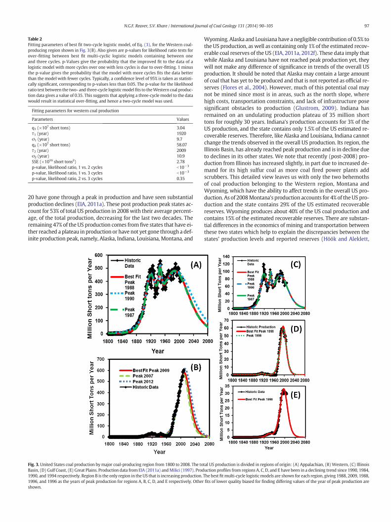
Table 2Fitting parameters of best fit two-cycle logistic model, of Eq. (3), for the Western coal-producing region shown in Fig. 3(B). Also given are p-values for likelihood ratio tests forover-fitting between best fit multi-cyclic logistic models containing between oneand three cycles. p-Values give the probability that the improved fit to the data of alogistic model with more cycles over one with less cycles is due to over-fitting. 1 minusthe p-value gives the probability that the model with more cycles fits the data betterthan the model with fewer cycles. Typically, a confidence level of 95% is taken as statisti-cally significant, corresponding to p-values less than 0.05. The p-value for the likelihoodratio test between the two- and three-cycle logisticmodel fits to theWestern coal produc-tion data gives a value of 0.35. This suggests that applying a three-cycle model to the datawould result in statistical over-fitting, and hence a two-cycle model was used.
Fitting parameters for western coal production
Parameters Values
q1 (×107 short tons) 3.04τ1 (year) 1920σ1 (year) 9.7q2 (×107 short tons) 58.07τ2 (year) 2009σ2 (year) 10.9SSE (×1016 short tons2) 2.78p-value, likelihood ratio, 1 vs. 2 cycles b10−3
p-value, likelihood ratio, 1 vs. 3 cycles b10−3
p-value, likelihood ratio, 2 vs. 3 cycles 0.35
97N.G.F. Reaver, S.V. Khare / International Journal of Coal Geology 131 (2014) 90–105
20 have gone through a peak in production and have seen substantialproduction declines (EIA, 2011a). These post production peak states ac-count for 53% of total US production in 2008with their average percent-age, of the total production, decreasing for the last two decades. Theremaining 47% of the US production comes from five states that have ei-ther reached a plateau in production or have not yet gone through a def-inite production peak, namely, Alaska, Indiana, Louisiana, Montana, and
Fig. 3. United States coal production bymajor coal-producing region from 1800 to 2008. The toBasin, (D) Gulf Coast, (E) Great Plains. Production data from EIA (2011a) andMilici (1997). Prod1990, and 1994 respectively. Region B is the only region in the US that is increasing production.1996, and 1996 as the years of peak production for regions A, B, C, D, and E respectively. Othershown.
Wyoming. Alaska and Louisiana have a negligible contribution of 0.5% tothe US production, as well as containing only 1% of the estimated recov-erable coal reserves of the US (EIA, 2011a, 2012f). These data imply thatwhile Alaska and Louisiana have not reached peak production yet, theywill not make any difference of significance in trends of the overall USproduction. It should be noted that Alaska may contain a large amountof coal that has yet to be produced and that is not reported as official re-serves (Flores et al., 2004). However, much of this potential coal maynot be mined since most is in areas, such as the north slope, wherehigh costs, transportation constraints, and lack of infrastructure posesignificant obstacles to production (Glustrom, 2009). Indiana hasremained on an undulating production plateau of 35 million shorttons for roughly 30 years. Indiana's production accounts for 3% of theUS production, and the state contains only 1.5% of the US estimated re-coverable reserves. Therefore, like Alaska and Louisiana, Indiana cannotchange the trends observed in the overall US production. Its region, theIllinois Basin, has already reached peak production and is in decline dueto declines in its other states. We note that recently (post-2008) pro-duction from Illinois has increased slightly, in part due to increased de-mand for its high sulfur coal as more coal fired power plants addscrubbers. This detailed view leaves us with only the two behemothsof coal production belonging to the Western region, Montana andWyoming, which have the ability to affect trends in the overall US pro-duction. As of 2008Montana's production accounts for 4% of the US pro-duction and the state contains 29% of the US estimated recoverablereserves. Wyoming produces about 40% of the US coal production andcontains 15% of the estimated recoverable reserves. There are substan-tial differences in the economics of mining and transportation betweenthese two states which help to explain the discrepancies between thestates' production levels and reported reserves (Höök and Aleklett,
tal US production is divided in regions of origin: (A) Appalachian, (B)Western, (C) Illinoisuction profiles from regions A, C, D, and E have been in a declining trend since 1990, 1984,The best fit multi-cycle logisticmodels are shown for each region, giving 1988, 2009, 1988,fits of lower quality biased for finding differing values of the year of peak production are

Fig. 4.United Kingdom (UK) coal production from 1830 to 2008. Production data from BP(2010) and Mitchell (1988). The data show a virtually complete logistic production cycleshowing the initial ascent in production followed by a maximum and then a continuousdecline. A single cycle logistic model, fitted using the entire production dataset, isshown, illustrating an excellent fit. Single cycle logistic models fitted using only produc-tion data prior to 25%, 50%, 75%, and 100% of the peak value of the best fit curve areshown. These fits demonstrate the accuracy of prediction of peak year of productiononce 50% of the peak production corresponding to exhaustion of approximately 14% oftotal reserves has occurred.
Fig. 5. Pennsylvania anthracite coal production from 1800 to 2008. Production data fromEIA (2011a) and Milici (1997). Pennsylvania anthracite coal has the highest energy con-tent of coals in the US. Production of anthracite has followed logistic production cycle inspite of large reported reserves. Single and two-cycle logistic models, fitted using the en-tire production dataset, are shown, illustrating excellent fits. Single cycle logistic modelsfitted using only production data prior to 25%, 50%, 75%, and 100% of the peak value ofthe best fit curve are shown. These fits demonstrate the accuracy of prediction of peakyear of production once 50% of the peak production corresponding to exhaustion of ap-proximately 14% of total reserves has occurred.
98 N.G.F. Reaver, S.V. Khare / International Journal of Coal Geology 131 (2014) 90–105
2009, 2010). Though year to year fluctuations do occur, these stateshave contributed to US production at substantial and increasing levelssince 1972 and at an accelerated rate since the combined productionof the remaining 23 US states peaked in 1990. From 1990 to 2008, USproduction excluding Wyoming and Montana has declined by 18%,from 800 to 650 million short tons per year, or by about 8 millionshort tons per year per year. For the US production to even remain con-stant in the next 20 years, Wyoming andMontana will have to increaseproduction by 32%, over their 2008 levels, to compensate this decline inthe rest of the US. These two states already account for 44% of total coalproduction. For them to increase production to 58% of the US total fromsuch high levels is a daunting challenge likely to remain unmet. A sim-ilar conclusion about the future of Wyoming andMontana coal produc-tion was reached by Höök and Aleklett (2009, 2010). Thus our analysisby individual states is consistentwith the picture of peak in US coal pro-duction in the next decade at the latest, if not earlier.
From our model predictions, along with the detailed analysis by en-ergy content, rank and regional distribution, has emerged a consistentpicture that US total coal production and energy produced from coalare at their maximum or near maximum and will go into permanentgeological decline in the next 10 years or so. No inconsistencies in theanalysis have emerged. We now turn our attention to the validity andaccuracy of the model predictions. To assess the uncertainties thatmay arise in themodel predictionswe have performed several sensitiv-ity tests which we address next.
3.2. Sensitivity tests for year of peak production
Of the 12 coal regions exhibiting a complete production cycle, theUKtotal coal and Pennsylvania anthracite coal production were chosen tovalidate the logistic fitting procedure. Several reasons underlie thesetwo choices. The best fit URR of the UK, 32 billion short tons, is compa-rable to the best fit URR of individual regions of the US, 65, 10, 2, 1.4,and 29 billion short tons for the Appalachian, Illinois Basin, Gulf Coast,Great Plains, and Western coal-producing regions, respectively. ThePennsylvania data give an analysis for only a specific rank of coal, name-ly anthracite. This helps us ascertain our model predictions for the pro-duction peaks and URR of the four individual ranks of coal. Also, both ofthese production profiles, the UK total coal and Pennsylvania anthracite,have essentially gone through a complete mining production cycle. Ineach case, production increased exponentially, reached a maximum,and then decreased. By purposefully restricting analyses to varying de-grees of incomplete data from these complete datasets, i.e. by usingearly portions of the total production profile as the input data for thefitting procedure, we can assess how well the fitted models match upto both the complete production data and the best model fit performedon the entire dataset.
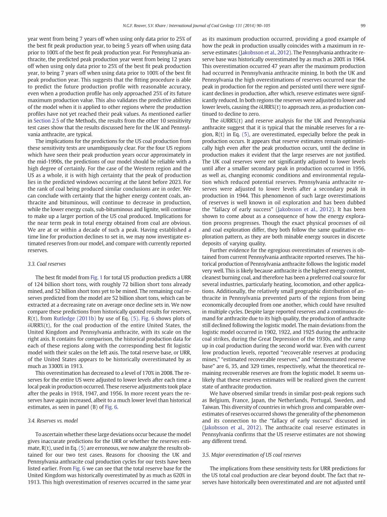
The results for the sensitivity and validation test of the logisticmodelfitting procedure are given in Fig. 4. Fig. 4 shows the UK coal productionfrom1830 to 2008. The production data showa virtually complete logis-tic production cycle showing the initial ascent in production followed bya maximum and then a continuous decline. The maximum productionof coal occurred in the year 1913 at 292 million metric tons per year.The best fit logistic model using the entire dataset gives a year of peakproduction at 1924, and amaximum production of 280.5 millionmetrictons per year. Also shown are best fit single cycle logistic models fittedusing only production data prior to 25%, 50%, 75%, and 100% of thepeak value of the best fit curve, giving peak years of 1931, 1915, 1916,and 1919 respectively. The maximum production levels, for the logisticmodels using data prior to 25%, 50%, 75%, and 100% of the peak value ofthe bestfitmodel are 405, 242, 228, and 256millionmetric tonsper yearrespectively.
The results of the second sensitivity and validation test are given inFig. 5. Shown is the Pennsylvania anthracite coal production from1800 to 2008. The production data show a virtually complete logisticproduction cycle, similar to the UK data. The actual production peaked
in the year 1917, at 99.6 million short tons per year. The best fit logisticmodel using the entire dataset gives a year of peak production at 1917,and a maximum production of 85 million short tons per year. Alsoshown are best fit single cycle logistic models fitted using only produc-tion data prior to 25%, 50%, 75%, and 100%of thepeak value of the best fitcurve, giving peak years of 1905, 1907, 1905, and 1924 respectively. Themaximum production levels, for the logistic models using data prior to25%, 50%, 75%, and 100% of the peak value of the best fit model are 87,66, 62, and 97 million short tons per year respectively.
For the UK, various fits performed on incomplete data predictedthe year of peak production to within ±9 years of the year of peakproduction obtained from the best fit using the entire dataset. For thePennsylvania anthracite, the fits performed predicted the year of peakproduction to within ±12 years of the peak production of the best fitmodel using the entire dataset. In both regions, the model had reducedaccuracy when the production profile was far earlier from the actualpeak in production. However, once the production profile approacheditsmaximum the accuracy improved. TheUKpredicted peak production
99N.G.F. Reaver, S.V. Khare / International Journal of Coal Geology 131 (2014) 90–105
year went from being 7 years off when using only data prior to 25% ofthe best fit peak production year, to being 5 years off when using dataprior to 100% of the best fit peak production year. For Pennsylvania an-thracite, the predicted peak production year went from being 12 yearsoff when using only data prior to 25% of the best fit peak productionyear, to being 7 years off when using data prior to 100% of the best fitpeak production year. This suggests that the fitting procedure is ableto predict the future production profile with reasonable accuracy,even when a production profile has only approached 25% of its futuremaximum production value. This also validates the predictive abilitiesof the model when it is applied to other regions where the productionprofiles have not yet reached their peak values. As mentioned earlierin Section 2.5 of the Methods, the results from the other 10 sensitivitytest cases show that the results discussed here for the UK and Pennsyl-vania anthracite, are typical.
The implications for the predictions for the US coal production fromthese sensitivity tests are unambiguously clear. For the four US regionswhich have seen their peak production years occur approximately inthe mid-1990s, the predictions of our model should be reliable with ahigh degree of certainly. For the case of the Western region and theUS as a whole, it is with high certainty that the peak of productionlies in the predicted windows occurring at the latest before 2023. Forthe rank of coal being produced similar conclusions are in order. Wecan conclude with certainty that the higher energy content coals, an-thracite and bituminous, will continue to decrease in production,while the lower energy coals, sub-bituminous and lignite, will continueto make up a larger portion of the US coal produced. Implications forthe near term peak in total energy obtained from coal are obvious.We are at or within a decade of such a peak. Having established atime line for production declines to set in, we may now investigate es-timated reserves from our model, and compare with currently reportedreserves.
3.3. Coal reserves
The best fit model from Fig. 1 for total US production predicts a URRof 124 billion short tons, with roughly 72 billion short tons alreadymined, and 52 billion short tons yet to bemined. The remaining coal re-serves predicted from the model are 52 billion short tons, which can beextracted at a decreasing rate on average once decline sets in. We nowcompare these predictions from historically quoted results for reserves,R(t), from Rutledge (2011b) by use of Eq. (5). Fig. 6 shows plots ofδURR%(t), for the coal production of the entire United States, theUnited Kingdom and Pennsylvania anthracite, with its scale on theright axis. It contains for comparison, the historical production data foreach of these regions along with the corresponding best fit logisticmodel with their scales on the left axis. The total reserve base, or URR,of the United States appears to be historically overestimated by asmuch as 3300% in 1913.
This overestimation has decreased to a level of 170% in 2008. The re-serves for the entire US were adjusted to lower levels after each time alocal peak in production occurred. These reserve adjustments took placeafter the peaks in 1918, 1947, and 1956. In more recent years the re-serves have again increased, albeit to a much lower level than historicalestimates, as seen in panel (B) of Fig. 6.
3.4. Reserves vs. model
To ascertainwhether these large deviations occur because themodelgives inaccurate predictions for the URR or whether the reserves esti-mate, R(t), used in Eq. (5) are erroneous, we now analyze the results ob-tained for our two test cases. Reasons for choosing the UK andPennsylvania anthracite coal production cycles for our tests have beenlisted earlier. From Fig. 6 we can see that the total reserve base for theUnited Kingdom was historically overestimated by as much as 620% in1913. This high overestimation of reserves occurred in the same year
as its maximum production occurred, providing a good example ofhow the peak in production usually coincides with a maximum in re-serve estimates (Jakobsson et al., 2012). The Pennsylvania anthracite re-serve base was historically overestimated by as much as 200% in 1964.This overestimation occurred 47 years after the maximum productionhad occurred in Pennsylvania anthracite mining. In both the UK andPennsylvania the high overestimations of reserves occurred near thepeak in production for the region and persisted until there were signif-icant declines in production, after which, reserve estimates were signif-icantly reduced. In both regions the reserveswere adjusted to lower andlower levels, causing the δURR%(t) to approach zero, as production con-tinued to decline to zero.
The δURR%(t) and reserve analysis for the UK and Pennsylvaniaanthracite suggest that it is typical that the minable reserves for a re-gion, R(t) in Eq. (5), are overestimated, especially before the peak inproduction occurs. It appears that reserve estimates remain optimisti-cally high even after the peak production occurs, until the decline inproduction makes it evident that the large reserves are not justified.The UK coal reserves were not significantly adjusted to lower levelsuntil after a smaller secondary peak in production occurred in 1956,as well as, changing economic conditions and environmental regula-tion which reduced potential reserves. Pennsylvania anthracite re-serves were adjusted to lower levels after a secondary peak inproduction in 1944. This phenomenon of such large overestimationsof reserves is well known in oil exploration and has been dubbedthe “fallacy of early success” (Jakobsson et al., 2012). It has beenshown to come about as a consequence of how the energy explora-tion process progresses. Though the exact physical processes of oiland coal exploration differ, they both follow the same qualitative ex-ploration pattern, as they are both minable energy sources in discretedeposits of varying quality.
Further evidence for the egregious overestimates of reserves is ob-tained from current Pennsylvania anthracite reported reserves. The his-torical production of Pennsylvania anthracite follows the logistic modelvery well. This is likely because anthracite is the highest energy content,cleanest burning coal, and therefore has been a preferred coal source forseveral industries, particularly heating, locomotion, and other applica-tions. Additionally, the relatively small geographic distribution of an-thracite in Pennsylvania prevented parts of the regions from beingeconomically decoupled from one another, which could have resultedin multiple cycles. Despite large reported reserves and a continuous de-mand for anthracite due to its high quality, the production of anthracitestill declined following the logistic model. Themain deviations from thelogistic model occurred in 1902, 1922, and 1925 during the anthracitecoal strikes, during the Great Depression of the 1930s, and the rampup in coal production during the second world war. Even with currentlow production levels, reported “recoverable reserves at producingmines,” “estimated recoverable reserves,” and “demonstrated reservebase” are 6, 35, and 329 times, respectively, what the theoretical re-maining recoverable reserves are from the logistic model. It seems un-likely that these reserves estimates will be realized given the currentstate of anthracite production.
We have observed similar trends in similar post-peak regions suchas Belgium, France, Japan, the Netherlands, Portugal, Sweden, andTaiwan. This diversity of countries in which gross and comparable over-estimates of reserves occurred shows the generality of the phenomenonand its connection to the “fallacy of early success” discussed in(Jakobsson et al., 2012). The anthracite coal reserve estimates inPennsylvania confirms that the US reserve estimates are not showingany different trend.
3.5. Major overestimation of US coal reserves
The implications from these sensitivity tests for URR predictions forthe US total coal production are clear beyond doubt. The fact that re-serves have historically been overestimated and are not adjusted until

Fig. 6. δURR%(t) for the Unites States (A) and (B, expanded view), the United Kingdom (C), and Pennsylvania anthracite coal production (D); right axis. Coal reserve data used to calculatethe δURR%(t) are from Rutledge (2011b). Also displayed are historical production data and best fits as described in Figs. 1, 4, and 5; left axis. δURR%(t) gives an approximate percentage ofover- or underestimated reserves as defined by Eq. (5). Both C andD have essentially completed a logistic production cycle allowing δURR%(t) to be directly calculated fromhistorical data,while the δURR%(t) for A is estimated using the best fit model. Panel B shows an expanded viewof A so that detail in the δURR%(t) ofmore recent years can be observed. It can be seen thatfor C and D that the total reserve base was historically overestimated by as much as 620% in 1913 and 200% in 1964, respectively. These high overestimations in reserves occurred near orafter the peak in the production of the coal region, and persisted until therewere significant declines in production, afterwhich, reserve estimateswere significantly reduced. In both C andD the reserves were adjusted to lower and lower levels, causing the δURR%(t) to approach zero, as production continued to decline to zero. It is shown that it is estimated that A also his-torically overestimated the total reserve base by as much as 3300% in 1913. As can be seen in B, this overestimation has decreased to a level of 170% by 2008.
100 N.G.F. Reaver, S.V. Khare / International Journal of Coal Geology 131 (2014) 90–105
peak and then declining production suggests that the current reportedUS reserve estimates from the EIA of 259 billion short tons (EIA,2012f) are a gross overestimate. Amore reasonable estimate is providedbyour bestfitmodel in Fig. 1 of 52billion short tons yet to bemined. Ourresult directly contradicts a commonly quoted assertion that there isenough coal supply to last the next 200–250 years. This statement is de-rived bydividing the reported EIA reserves of 259billion short tons (EIA,2012f) by the current production of about 1.1 billion short tons to obtain235 years. However, such a “reserves-to-production” estimate relies ontwo assumptions. The first of which is that a high constant productionrate can be maintained. Decades of data from real coal production pro-files from around the world show that these profiles do resemble ingeneral form, though do not follow exactly, the ideal multi-cyclic logis-tic type curves of our model. Therefore production goes into declinelong before reserves are exhausted or when approximately 50% of theactual reserves have been produced. Thus the first assumption is clearlyin error. The second assumption is that the reported reserves are accu-rate which our sensitivity analysis clearly shows to be false. Thus, ourfindings not merely echo, but also provide quantitative analysis to con-firm, the statements made by the National Research Council in their2007 report on coal, “However, it is not possible to confirm the often-quoted assertion that there is a sufficient supply of coal for the next250 years” (NRC, 2007). The summary conclusion of our work is thatthe US has a reserves-to-production ratio of approximately 47 yearsand not 200–250 years as often quoted (AP, 2013; CN, 2013; IER,2013; Katzer et al., 2007; Milici, 1996).
3.6. Comparison to previous results
Our results are comparable to those of prior work on forecasting UScoal production that we described in Section 2.1 Forecasting and Prior
Work. Here we use the metric units gigatons (Gt), megatons (Mt), andexajoules (EJ), so results can be easily compared between studies. Theresults of our best fit and lower quality biased fits of themulti-cyclic lo-gistic model fitting process give a range of values for the peak produc-tion year, maximum production rate, and URR for both coal rawtonnage and energy.
For coal raw tonnage, these ranges are: 2009–2023 for the peak pro-duction year, 1.14–1.28 billion short tons per year, or equivalently,1035–1163 Mt per year for the maximum production rate, and 124–162 billion short tons, or equivalently, 112–147 Gt for the URR.
For energy from coal, these ranges are: 2003–2018 for the peak pro-duction year, 23.1–25.2 quadrillion BTU per year, or equivalently, 24.3–26.6 EJ per year for themaximum production rate, and 2557–3430 qua-drillion BTU, or equivalently, 2698–3619 EJ for the URR.
The study by Rutledge provides estimates of the coal tonnage URRfor US divided into three regions, Eastern, Western, and Pennsylvaniaanthracite (Rutledge, 2011a). The estimatedURRs for the Eastern,West-ern, and Pennsylvania anthracite regions are 82 Gt, 45 Gt, and 5.05 Gt,respectively, giving a total US URR of 132.05 Gt. This value is in goodagreement with our results as it lies within our estimated range of112–147 Gt for the US URR.
The study by Patzek and Croft provides estimates for the peak pro-duction year, maximum production rate, and URR for energy from UScoal (Patzek and Croft, 2010). The values are 2015 for the peak produc-tion year, 26.8 EJ per year for the maximum production rate, and 2757EJ for the URR. These values are in close agreement with our resultsfor energy from US coal. Their peak production year of 2015 and URRof 2757 EJ lie within our estimated ranges of 2003–2018 for the peakproduction year and 2698–3618 EJ for the URR. Their estimate of themaximum production rate, 26.8 EJ per year, is close to the high side ofour estimated range of 24.3–26.6 EJ per year.

101N.G.F. Reaver, S.V. Khare / International Journal of Coal Geology 131 (2014) 90–105
The study by Mohr and Evans provides estimates for the peak pro-duction year, maximum production rate, and URR for US coal ton-nage, using several methods (S. Mohr and Evans, 2009). Here wecompare the results of the Hubbert Linearization and Best Guess sce-narios in their paper to our results. The results of the Hubbert Linear-ization give estimates of 2005 for the peak production year, 1232 Mtper year for the maximum production rate, and 171.7 Gt for the URR.Their Best Guess scenario gives 2048 for the peak production year,1809 Mt per year for the maximum production rate, and 308.1 Gtfor the URR. Both of the methods produced URRs and maximum pro-duction rates larger than those in our results, which were 112.5–147.4 Gt and 1035–1163 Mt per year, respectively. The Hubbert Line-arization used in S. Mohr and Evans (2009) gave a peak productionyear that is earlier our results, 2005 vs. 2009–2023, while their BestGuess scenario gave a peak production year later than our results,2048. The results from this study did not align with our results asclosely as other studies, however, they still support the common con-clusion that the US does not have a 200 or 250 year supply of coalremaining.
The study by the Energy Watch Group provides estimates for thepeak production year and maximum production rate for US coal.Their analysis suggests that US coal production by tonnage willpeak between the years 2020 and 2030. This range overlaps withour results of US coal production reaching peak between the years2009 and 2023. The Energy Watch Group study also estimates thatthe maximum production rate at peak in terms of energy will be atmost 20% higher than 2007 production levels. This corresponds to arate of 27.9 EJ per year, which is close to the high side of our estimat-ed range of 24.3–26.6 EJ per year.
The study by Glustrom concludes that the “planning horizon formoving beyond coal could be as short as 20–30 years” (Glustrom,2009). This time frame agrees with our results which suggest animminent peak in US coal tonnage production between 2009 at2023. The Glustrom study also found that the western states ofWyoming and Montana will dominate future production, similarto our findings.
The studies by Höök and Aleklett and Höök et al. provide esti-mates several scenarios of future US coal production (Höök andAleklett, 2009, 2010; Höök et al., 2010). Their analysis found thatthe US states of Wyoming and Montana will ultimately control thegrowth and decline of future US production, as we did in our analysis.In each of the studies they suggest that if the large reported reservesof Montana are not fully exploited US production will likely peak be-fore 2050, likely around 2030. Their analysis found that the maximumrate of production of US coal will likely reach 1400 Mt per year andmaintain that level until the end of the century if the US's large re-ported reserves are developed, or slowly decline if the reserves areoverestimated. The results from their studies gave later peak yearsand larger production rates than our results, however, they still sup-port the common conclusion that the US does not have a 200 or250 year supply of coal remaining.
These studies all used a variety of different analysis and forecastingmethods, as described in Section 2.1, and still came to similar conclu-sions that US coal production will likely be significantly less than whatis suggested by the currently reported reserves. Our results agree closelywith those of many of the studies, and agree with the common conclu-sion of a limited US coal supply that all of these studies came to. Thisagreement lends support to the validity of our results.
3.7. Ancillary evidence of peak production
It is clear from the data presented on individual regions and statesthat the Western region, particularly Wyoming and Montana, will de-termine when the entire US will reach peak production. Furthermore,to compensate for the decline in combined production from the other23 states, these two states have to increase their production rate
in the future. Ancillary data about (i) stripping ratio (BLM, 2013;Glustrom, 2009), (ii) US coal mine-worker productivity (EIA, 2012c)and (iii) energy returned on energy invested data (EROEI) (Cleveland,1992; Gupta and Hall, 2011; Hall and Cleveland, 1981; Hall et al.,1986) are consistent with ourmodel predictions for a peak of US energyproduction to be approaching soon, i.e. within a decade or earlier. Webriefly discuss each of these here.
(i) Themajority of the large producingmines in these two states aresurfacemines locatedwithin the Powder River Basin (EIA, 2012g;USGS, 2013). For surfacemines ameasure known as the strippingratio is important for determining the economics and feasibilityof mining. The stripping ratio is the amount of overburden (i.e.the rock or soil above the coal) that needs to be removed to ob-tain an amount of coal. Larger stripping ratios may make surfacemining uneconomical, as the costs to remove the excess overbur-den can become too large to make the operation profitable. Thestripping of waste rock and soil make up a significant portion ofthe cost of production for a mine (Thompson, 2005). Additional-ly, larger stripping ratios do not increase productions costs line-arly, but rather exponentially (Shafiee et al., 2009). This meansa small increase in stripping ratio can quickly make mining un-economical. The current producing mines in the Powder RiverBasin are on the edges of the basinwhere the overburden is thin-nest (DOE, 2007; Glustrom, 2009; USGS, 2013). The USGS hassignificantly reduced the size of the estimated recoverable re-serves in the Powder River Basin in part due to much of thecoal having large stripping ratios (Glustrom, 2009; Luppenset al., 2008). As the coal with low stripping ratio is depleted,the coal remaininghas a higher stripping ratio. Future productionwill come from higher stripping ratio mines leading to less netenergy obtained from the coal.
(ii) The worker productivity of a coal mine is an important mea-sure for its profitability and will reflect the cost of coal pro-duced at the mine. The more short tons of coal that can bemined per employee hour the more profitable the mine canbe. As mines deplete (e.g. thinner coal seams), or the coal be-comes harder to access (e.g. larger strip ratios), less coal can beproduced for the same amount of time and effort. The overallaverage mine productivity of the US is therefore an indicatorfor the state of depletion of US coal resources and the qualityof remaining coal resources. US mine productivity increasedfrom approximately 2 short tons per employee hour in theyear 1980 to a peak of 7 short tons per employee hour in theyear 2000, coinciding with major increases in productionfrom primarily surface mining in the Western region, particu-larly Wyoming. Since then the average coal mine productivityhas been in a decreasing trend and has dropped to a level of6 short tons per employee hour by 2008, a decrease of 15%.The mine productively in terms of energy from coal shows amore pronounced decrease in productivity since the peak in2000. Mine productivity has gone from 147 million BTU peremployee hour in 2000 to 121 million BTU per employeehour in 2008, a decrease of 18%. This is due to the continuousdecline in the energy content of US coals, as was also found in(Höök and Aleklett, 2009; Zittel and Schindler, 2007), as wellas, supports our findings that the US will reach peak in energyin coal before tonnage from coal. The timing of this peak inproductivity in the year 2000 mirrors the timing of the USreaching a plateau in energy production from coal in 1997.
(iii) EROEI is a form of energy balance of an energy resource. It repre-sents the amount of energy that is obtained for every unit of en-ergy invested in producing that energy source. The higher theEROEI of an energy resource, the greater net energy the sourcecan provide to run the economy and society at large. Thismeans that the EROEI is a measure of a type of quality for an
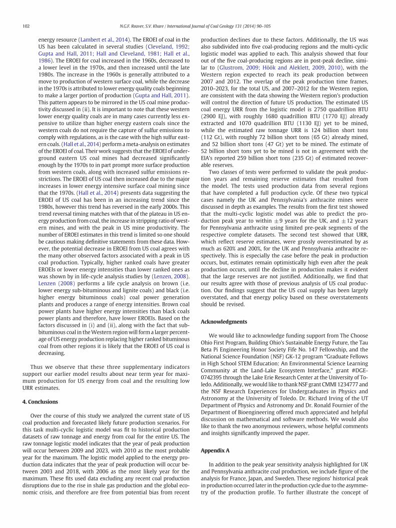
102 N.G.F. Reaver, S.V. Khare / International Journal of Coal Geology 131 (2014) 90–105
energy resource (Lambert et al., 2014). The EROEI of coal in theUS has been calculated in several studies (Cleveland, 1992;Gupta and Hall, 2011; Hall and Cleveland, 1981; Hall et al.,1986). The EROEI for coal increased in the 1960s, decreased toa lower level in the 1970s, and then increased until the late1980s. The increase in the 1960s is generally attributed to amove to production of western surface coal, while the decreasein the 1970s is attributed to lower energy quality coals beginningto make a larger portion of production (Gupta and Hall, 2011).This pattern appears to be mirrored in the US coal mine produc-tivity discussed in (ii). It is important to note that these westernlower energy quality coals are in many cases currently less ex-pensive to utilize than higher energy eastern coals since thewestern coals do not require the capture of sulfur emissions tocomply with regulations, as is the case with the high sulfur east-ern coals. (Hall et al., 2014) perform ameta-analysis on estimatesof the EROEI of coal. Theirwork suggests that the EROEI of under-ground eastern US coal mines had decreased significantlyenough by the 1970s to in part prompt more surface productionfrom western coals, along with increased sulfur emissions re-strictions. The EROEI of US coal then increased due to the majorincreases in lower energy intensive surface coal mining sincethat the 1970s. (Hall et al., 2014) presents data suggesting theEROEI of US coal has been in an increasing trend since the1980s, however this trend has reversed in the early 2000s. Thistrend reversal timing matches with that of the plateau in US en-ergy production from coal, the increase in stripping ratio ofwest-ern mines, and with the peak in US mine productivity. Thenumber of EROEI estimates in this trend is limited so one shouldbe cautious making definitive statements from these data. How-ever, the potential decrease in EROEI from US coal agrees withthe many other observed factors associated with a peak in UScoal production. Typically, higher ranked coals have greaterEROEIs or lower energy intensities than lower ranked ones aswas shown by in life-cycle analysis studies by (Lenzen, 2008).Lenzen (2008) performs a life cycle analysis on brown (i.e.lower energy sub-bituminous and lignite coals) and black (i.e.higher energy bituminous coals) coal power generationplants and produces a range of energy intensities. Brown coalpower plants have higher energy intensities than black coalspower plants and therefore, have lower EROEIs. Based on thefactors discussed in (i) and (ii), along with the fact that sub-bituminous coal in theWestern regionwill forma larger percent-age of US energy production replacing higher ranked bituminouscoal from other regions it is likely that the EROEI of US coal isdecreasing.
Thus we observe that these three supplementary indicatorssupport our earlier model results about near term year for maxi-mum production for US energy from coal and the resulting lowURR estimates.
4. Conclusions
Over the course of this study we analyzed the current state of UScoal production and forecasted likely future production scenarios. Forthis task multi-cyclic logistic model was fit to historical productiondatasets of raw tonnage and energy from coal for the entire US. Theraw tonnage logistic model indicates that the year of peak productionwill occur between 2009 and 2023, with 2010 as the most probableyear for the maximum. The logistic model applied to the energy pro-duction data indicates that the year of peak production will occur be-tween 2003 and 2018, with 2006 as the most likely year for themaximum. These fits used data excluding any recent coal productiondisruptions due to the rise in shale gas production and the global eco-nomic crisis, and therefore are free from potential bias from recent
production declines due to these factors. Additionally, the US wasalso subdivided into five coal-producing regions and the multi-cycliclogistic model was applied to each. This analysis showed that fourout of the five coal-producing regions are in post-peak decline, simi-lar to (Glustrom, 2009; Höök and Aleklett, 2009, 2010), with theWestern region expected to reach its peak production between2007 and 2012. The overlap of the peak production time frames,2010–2023, for the total US, and 2007–2012 for the Western region,are consistent with the data showing the Western region's productionwill control the direction of future US production. The estimated UScoal energy URR from the logistic model is 2750 quadrillion BTU(2900 EJ), with roughly 1680 quadrillion BTU (1770 EJ) alreadyextracted and 1070 quadrillion BTU (1130 EJ) yet to be mined,while the estimated raw tonnage URR is 124 billion short tons(112 Gt), with roughly 72 billion short tons (65 Gt) already mined,and 52 billion short tons (47 Gt) yet to be mined. The estimate of52 billion short tons yet to be mined is not in agreement with theEIA's reported 259 billion short tons (235 Gt) of estimated recover-able reserves.
Two classes of tests were performed to validate the peak produc-tion years and remaining reserve estimates that resulted fromthe model. The tests used production data from several regionsthat have completed a full production cycle. Of these two typicalcases namely the UK and Pennsylvania's anthracite mines werediscussed in depth as examples. The results from the first test showedthat the multi-cyclic logistic model was able to predict the pro-duction peak year to within ±9 years for the UK, and ±12 yearsfor Pennsylvania anthracite using limited pre-peak segments of therespective complete datasets. The second test showed that URR,which reflect reserve estimates, were grossly overestimated by asmuch as 620% and 200%, for the UK and Pennsylvania anthracite re-spectively. This is especially the case before the peak in productionoccurs, but, estimates remain optimistically high even after the peakproduction occurs, until the decline in production makes it evidentthat the large reserves are not justified. Additionally, we find thatour results agree with those of previous analysis of US coal produc-tion. Our findings suggest that the US coal supply has been largelyoverstated, and that energy policy based on these overstatementsshould be revised.
Acknowledgments
We would like to acknowledge funding support from The ChooseOhio First Program, Building Ohio's Sustainable Energy Future, the TauBeta Pi Engineering Honor Society Fife No. 147 Fellowship, and theNational Science Foundation (NSF) GK-12 program “Graduate Fellowsin High School STEM Education: An Environmental Science LearningCommunity at the Land-Lake Ecosystem Interface,” grant #DGE-0742395 through the Lake Erie Research Center at the University of To-ledo. Additionally,wewould like to thankNSF grant CMMI 1234777 andthe NSF Research Experiences for Undergraduates in Physics andAstronomy at the University of Toledo. Dr. Richard Irving of the UTDepartment of Physics and Astronomy and Dr. Ronald Fournier of theDepartment of Bioengineering offered much appreciated and helpfuldiscussion on mathematical and software methods. We would alsolike to thank the two anonymous reviewers, whose helpful commentsand insights significantly improved the paper.
Appendix A
In addition to the peak year sensitivity analysis highlighted for UKand Pennsylvania anthracite coal production, we include figure of theanalysis for France, Japan, and Sweden. These regions' historical peakin production occurred later in the production cycle due to the asymme-try of the production profile. To further illustrate the concept of

103N.G.F. Reaver, S.V. Khare / International Journal of Coal Geology 131 (2014) 90–105
historical gross overestimation of URR and reserves, we also include fig-ures for the δURR%(t) analysis for these three regions.
Fig. A1. French coal production from 1787 to 2006. Production data from S.H. Mohr andEvans (2009). The data show a virtually complete production cycle. A single cycle logisticmodel, fitted using the entire production dataset, is shown. Single cycle logistic modelsfitted using only production data prior to 25%, 50%, 75%, and 100% of the peak value ofthe best fit curve are shown.
Fig. A2. Japanese coal production from 1874 to 2006. Production data from S.H. Mohr andEvans (2009). The data show a virtually complete production cycle. A single cycle logisticmodel, fitted using the entire production dataset, is shown. Single cycle logistic modelsfitted using only production data prior to 25%, 50%, 75%, and 100% of the peak value ofthe best fit curve are shown.
Fig. A3. Swedish coal production from 1850 to 2006. Production data from S.H. Mohr andEvans, 2009). The data show a virtually complete production cycle. A single cycle logisticmodel, fitted using the entire production dataset, is shown. Single cycle logistic modelsfitted using only production data prior to 25%, 50%, 75%, and 100% of the peak value ofthe best fit curve are shown.
Fig. A4. δURR%(t) for France; right axis. Coal reserve data used to calculate the δURR%(t)are from Rutledge (2011b). Also displayed are historical production data and best fits;left axis. δURR%(t) gives an approximate percentage of over- or underestimated reservesas defined by Eq. (5). France has essentially completed a logistic production cycle allowingδURR%(t) to be directly calculated from historical data. It can be seen that the total reservebase was historically overestimated by as much as 360% in 1936. These high overestima-tions in reserves occurred near or after the peak in the production of the coal region,and persisted until there were significant declines in production, after which, reserve es-timates were significantly reduced. The reserves were adjusted to lower and lower levels,causing the δURR%(t) to approach zero, as production continued to decline to zero.
Fig. A5. δURR%(t) for Japan; right axis. Coal reserve data used to calculate the δURR%(t) arefrom Rutledge (2011b). Also displayed are historical production data and best fits; leftaxis. δURR%(t) gives an approximate percentage of over- or underestimated reserves asdefined by Eq. (5). Japan has essentially completed a logistic production cycle allowingδURR%(t) to be directly calculated from historical data. It can be seen that the total reservebase was historically overestimated by as much as 700% in 1968. These high overestima-tions in reserves occurred near or after the peak in the production of the coal region,and persisted until there were significant declines in production, after which, reserve es-timates were significantly reduced. The reserves were adjusted to lower and lower levels,causing the δURR%(t) to approach zero, as production continued to decline to zero.
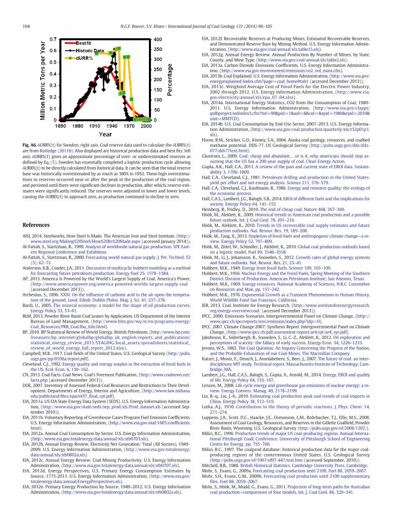
Fig. A6. δURR%(t) for Sweden; right axis. Coal reserve data used to calculate the δURR%(t)are from Rutledge (2011b). Also displayed are historical production data and best fits; leftaxis. δURR%(t) gives an approximate percentage of over- or underestimated reserves asdefined by Eq. (5). Sweden has essentially completed a logistic production cycle allowingδURR%(t) to be directly calculated from historical data. It can be seen that the total reservebase was historically overestimated by as much as 360% in 1952. These high overestima-tions in reserves occurred near or after the peak in the production of the coal region,and persisted until therewere significant declines in production, after which, reserve esti-mates were significantly reduced. The reserves were adjusted to lower and lower levels,causing the δURR%(t) to approach zero, as production continued to decline to zero.
104 N.G.F. Reaver, S.V. Khare / International Journal of Coal Geology 131 (2014) 90–105
References
AISI, 2014. Steelworks, How Steel Is Made. The American Iron and Steel Institute, (http://www.steel.org/Making%20Steel/How%20Its%20Made.aspx (accessed January 2014)).
Al-Fattah, S., Startzman, R., 1999. Analysis of worldwide natural gas production. SPE East-ern Regional Conference and Exhibition.
Al-Fattah, S., Startzman, R., 2000. Forecasting world natural gas supply. J. Pet. Technol. 52(5), 62–72.
Anderson, K.B., Conder, J.A., 2011. Discussion of multicyclic hubbert modeling as amethodfor forecasting future petroleum production. Energy Fuel 25, 1578–1584.
AP, 2013. America Is Powered by the World's Largest Supply of Coal. America's Power,(http://www.americaspower.org/america-powered-worlds-largest-supply-coal(accessed December 2013)).
Arrhenius, S., 1896. XXXI. On the influence of carbonic acid in the air upon the tempera-ture of the ground. Lond. Edinb. Dublin Philos. Mag. J. Sci. 41, 237–276.
Bardi, U., 2005. The mineral economy: a model for the shape of oil production curves.Energy Policy 33, 53–61.
BLM, 2013. Powder River Basin Coal Leases by Application. US Department of the InteriorBureau of Land Management, (http://www.blm.gov/wy/st/en/programs/energy/Coal_Resources/PRB_Coal/lba_title.html).
BP, 2010. BP Statistical Review of World Energy. British Petroleum, (http://www.bp.com/liveassets/bp_internet/globalbp/globalbp_uk_english/reports_and_publications/statistical_energy_review_2011/STAGING/local_assets/spreadsheets/statistical_review_of_world_energy_full_report_2012.xlsx).
Campbell, M.R., 1917. Coal fields of the United States. U.S. Geological Survey (http://pubs.usgs.gov/pp/0100a/report.pdf).
Cleveland, C.J., 1992. Energy quality and energy surplus in the extraction of fossil fuels inthe US. Ecol. Econ. 6, 139–162.
CN, 2013. Coal Facts. Coal News. Coal's Foremost Publication, (http://www.coalnews.net/facts.php (accessed December 2013)).
DOE, 2007. Inventory of Assessed Federal Coal Resources and Restrictions to Their Devel-opment. Departments of Energy, Interior and Agriculture, (http://www.law.indiana.edu/publicland/files/epact437_final_rpt.pdf).
EIA, 2011a. US EIA State Energy Data System (SEDS). U.S. Energy Information Administra-tion, (http://www.eia.gov/state/seds/sep_prod/xls/Prod_dataset.xls (accessed Sep-tember 2010)).
EIA, 2011b. Voluntary Reporting of Greenhouse Gases Program Fuel Emission Coefficients.U.S. Energy Information Administration, (http://www.eia.gov/oiaf/1605/coefficients.html).
EIA, 2012a. Annual Coal Consumption by Sector. U.S. Energy Information Administration,(http://www.eia.gov/totalenergy/data/annual/xls/stb0703.xls).
EIA, 2012b. Annual Energy Review, Electricity Net Generation: Total (All Sectors), 1949–2009. U.S. Energy Information Administration, (http://www.eia.gov/totalenergy/data/annual/xls/stb0802a.xls).
EIA, 2012c. Annual Energy Review: Coal Mining Productivity. U.S. Energy InformationAdministration, (http://www.eia.gov/totalenergy/data/annual/xls/stb0707.xls).
EIA, 2012d. Energy Perspectives, U.S. Primary Energy Consumption Estimates bySource, 1775-2011. U.S. Energy Information Administration, (http://www.eia.gov/totalenergy/data/annual/EnergyPerspectives.xls).
EIA, 2012e. Primary Energy Production by Source, 1949–2012. U.S. Energy InformationAdministration, (http://www.eia.gov/totalenergy/data/annual/xls/stb0802a.xls).
EIA, 2012f. Recoverable Reserves at Producing Mines, Estimated Recoverable Reserves,and Demonstrated Reserve Base by Mining Method. U.S. Energy Information Admin-istration, (http://www.eia.gov/coal/annual/xls/table15.xls).
EIA, 2012g. Annual Energy Review. Annual Production By Number of Mines, by State,County, and Mine Type, (http://www.eia.gov/coal/annual/xls/table2.xls).
EIA, 2013a. Carbon Dioxide Emissions Coefficients. U.S. Energy Information Administra-tion, (http://www.eia.gov/environment/emissions/co2_vol_mass.cfm).
EIA, 2013b. Coal Explained. U.S. Energy Information Administration, (http://www.eia.gov/energyexplained/index.cfm?page=coal_home#tab1 (accessed December 2013)).
EIA, 2013c. Weighted Average Cost of Fossil Fuels for the Electric Power Industry,2002 through 2012. U.S. Energy Information Administration, (http://www.eia.gov/electricity/annual/xls/epa_07_04.xlsx).
EIA, 2014a. International Energy Statistics, CO2 from the Consumption of Coal, 1980-2011. U.S. Energy Information Administration, (http://www.eia.gov/cfapps/ipdbproject/iedindex3.cfm?tid=90&pid=1&aid=8&cid=&syid=1980&eyid=2010&unit=MMTCD).
EIA, 2014b. U.S. Coal Consumption by End-Use Sector, 2007–2013. U.S. Energy Informa-tion Administration, (http://www.eia.gov/coal/production/quarterly/xls/t32p01p1.xls).
Flores, R.M., Stricker, G.D., Kinney, S.A., 2004. Alaska coal geology, resources, and coalbedmethane potential. DDS-77, US Geological Survey (http://pubs.usgs.gov/dds/dds-077/dds77text.html).
Glustrom, L., 2009. Coal: cheap and abundant… or is it, why americans should stop as-suming that the US has a 200-year supply of coal. Clean Energy Action.
Gupta, A.K., Hall, C.A., 2011. A review of the past and current state of EROI data. Sustain-ability 3, 1796–1809.
Hall, C.A., Cleveland, C.J., 1981. Petroleum drilling and production in the United States:yield per effort and net energy analysis. Science 211, 576–579.
Hall, C.A., Cleveland, C.J., Kaufmann, R., 1986. Energy and resource quality: the ecology ofthe economic process.
Hall, C.A.S., Lambert, J.G., Balogh, S.B., 2014. EROI of different fuels and the implications forsociety. Energy Policy 64, 141–152.
Heinberg, R., Fridley, D., 2010. The end of cheap coal. Nature 468, 367–369.Höök, M., Aleklett, K., 2009. Historical trends in American coal production and a possible
future outlook. Int. J. Coal Geol. 78, 201–216.Höök, M., Aleklett, K., 2010. Trends in US recoverable coal supply estimates and future
production outlooks. Nat. Resour. Res. 19, 189–208.Höök,M., Tang, X., 2013. Depletion of fossil fuels and anthropogenic climate change—a re-
view. Energy Policy 52, 797–809.Höök, M., Zittel, W., Schindler, J., Aleklett, K., 2010. Global coal production outlooks based
on a logistic model. Fuel 89, 3546–3558.Höök, M., Li, J., Johansson, K., Snowden, S., 2012. Growth rates of global energy systems
and future outlooks. Nat. Resour. Res. 21, 23–41.Hubbert, M.K., 1949. Energy from fossil fuels. Science 109, 103–109.Hubbert, M.K., 1956. Nuclear Energy and the Fossil Fuels, Spring Meeting of the Southern
District Division of Production. American Petroleum Institute, San Antonio, Texas.Hubbert, M.K., 1969. Energy resources. National Academy of Sciences, N.R.C. Committee
on Resources and Man, pp. 157–242.Hubbert, M.K., 1976. Exponential Growth as a Transient Phenomenon in Human History.
World Wildlife Fund San Francisco, California.IER, 2013. Coal. Institute for Energy Research, (http://www.instituteforenergyresearch.
org/energy-overview/coal/ (accessed December 2013)).IPCC, 2000. Emissions Scenarios. Intergovernmental Panel on Climate Change, (http://
www.ipcc.ch/ipccreports/sres/emission/index.php?idp=0).IPCC, 2007. Climate Change 2007: Synthesis Report. Intergovernmental Panel on Climate
Change, (http://www.ipcc.ch/pdf/assessment-report/ar4/syr/ar4_syr.pdf).Jakobsson, K., Söderbergh, B., Snowden, S., Li, C.-Z., Aleklett, K., 2012. Oil exploration and
perceptions of scarcity: the fallacy of early success. Energy Econ. 34, 1226–1233.Jevons, W.S., 1865. The Coal Question: An Inquiry Concerning the Progress of the Nation,
and the Probable Exhaustion of our Coal-Mines. The Macmillan Company.Katzer, J., Moniz, E., Deutch, J., Ansolabehere, S., Beer, J., 2007. The future of coal: an inter-
disciplinary MIT study. Technical report. Massachusetts Institute of Technology, Cam-bridge, MA.
Lambert, J.G., Hall, C.A.S., Balogh, S., Gupta, A., Arnold, M., 2014. Energy, EROI and qualityof life. Energy Policy 64, 153–167.
Lenzen, M., 2008. Life cycle energy and greenhouse gas emissions of nuclear energy: a re-view. Energy Convers. Manag. 49, 2178–2199.
Lin, B.-q., Liu, J.-h., 2010. Estimating coal production peak and trends of coal imports inChina. Energy Policy 38, 512–519.
Lotka, A.J., 1910. Contribution to the theory of periodic reactions. J. Phys. Chem. 14,271–274.
Luppens, J.A., Scott, D.C., Haacke, J.E., Osmonson, L.M., Rohrbacher, T.J., Ellis, M.S., 2008.Assessment of Coal Geology, Resources, and Reserves in the Gillette Coalfield, PowderRiver Basin, Wyoming. U.S. Geological Survey (http://pubs.usgs.gov/of/2008/1202/).
Milici, R.C., 1996. Production trends of major US coal-producing regions. Annual Interna-tional Pittsburgh CoalL Conference. University of Pittsburgh School of EngineeringCentre for Energy, pp. 755–760.
Milici, R.C., 1997. The coalprod database: historical production data for the major coal-producing regions of the conterminous United States. U.S. Geological Survey(http://pubs.usgs.gov/of/1997/of97-447/text.htm (accessed September, 2010)).
Mitchell, B.R., 1988. British Historical Statistics. Cambridge University Press, Cambridge.Mohr, S., Evans, G., 2009a. Forecasting coal production until 2100. Fuel 88, 2059–2067.Mohr, S.H., Evans, G.M., 2009b. Forecasting coal production until 2100 supplementary
files. Fuel 88, 2059–2067.Mohr, S., Höök, M., Mudd, G., Evans, G., 2011. Projection of long-term paths for Australian
coal production—comparisons of four models. Int. J. Coal Geol. 86, 329–341.

105N.G.F. Reaver, S.V. Khare / International Journal of Coal Geology 131 (2014) 90–105
Moomaw, W., Burgherr P., Heath, G., Lenzen, M., Nyboer, J., Verbruggen, A., 2011. AnnexII: Methodology IPCC: Special Report on Renewable Energy Sources and ClimateChange Mitigation. Intergovernmental Panel on Climate Change, p. 982 (http://srren.ipcc-wg3.de/report/IPCC_SRREN_Annex_II.pdf).
Nashawi, I.S., Malallah, A., Al-Bisharah, M., 2010. Forecasting world crude oil productionusing multicyclic Hubbert model. Energy Fuel 24, 1788–1800.
NETL, 2012. Tracking New Coal-Fired Power Plants. National Energy Technology Labora-tory, p. 10 (http://www.netl.doe.gov/coal/refshelf/ncp.pdf).
NRC, 2007. Coal: Research and Development to Support National Energy Policy. NationalResearch Council, p. 4.
Patzek, T.W., Croft, G.D., 2010. A global coal production forecast with multi-Hubbert cycleanalysis. Energy 35, 3109–3122.
Rutledge, D., 2011a. Estimating long-term world coal production with logit and probittransforms. Int. J. Coal Geol. 85, 23–33.
Rutledge, D., 2011b. Estimating Long-Term World Coal Production with Logit and ProbitTransforms Excel Supplement.
Schweinfurth, S.P., 2009. The national coal resource assessment overview. U. S. Geol. Surv.12.
Shafiee, S., Nehring, M., Topal, E., 2009. Estimating average total cost of open pit coalmines in Australia. Aust. Min. 134.
Tao, Z., Li, M., 2007. What is the limit of Chinese coal supplies—a STELLAmodel of HubbertPeak. Energy Policy 35, 3145–3154.
Thompson, R.J., 2005. Surface Strip Coal Mining Handbook. South African CollieryManagers Association.
USGS, 1909. Papers on the conservation of mineral resources reprinted from report of theNational Conservation Commission. U.S. Geological Survey (http://pubs.usgs.gov/bul/0394/report.pdf).
USGS, 2013. USGS assessment of coal geology, resources, and reserve base in the powderriver basin, Wyoming and Montana. U.S. Geological Survey (http://pubs.usgs.gov/fs/2012/3143/fs-2012-3143.pdf).
USGS, 2014a. Iron and steel statistics and information. U.S. Geological Survey (http://min-erals.usgs.gov/minerals/pubs/commodity/iron_&_steel/).
USGS, 2014b. National coal resource data systems state cooperatives project. U.S. Geolog-ical Survey (http://energy.usgs.gov/Coal/StateCooperators.aspx (accessed September2010)).
Verhulst, P.-F., 1845. Recherches mathématiques sur la loi d'accroissement de la popula-tion. Nouveaux mém. l'acad. roy. sci. belles-lettres Bruxelles 18, 14–54.
Wang, J., Feng, L., Davidsson, S., Höök, M., 2013. Chinese coal supply and future produc-tion outlooks. Energy 60, 204–214.
WCA, 2014. Coal & Steel. World Coal Association, (http://www.worldcoal.org/coal/uses-of-coal/coal-steel/ (accessed January 2014)).
Zittel, W., Schindler, J., 2007. Coal: Resources and Future Production: Background Paper,EWG-Series. Energy Watch Group, (http://energywatchgroup.org/wp-content/uploads/2014/02/EWG_Report_Coal_10-07-2007ms1.pdf).