International Journal of Advanced and Applied Sciences, 7(2) 2020, Pages: 99-112

Contents lists available at Science-Gate

International Journal of Advanced and Applied Sciences Journal homepage: http://www.science-gate.com/IJAAS.html

99

Evaluation of water quality parameters using numerical modeling approach for the El-Salam Canal in Egypt

Walid M. A. Khalifa 1, 2, * 1Civil Engineering Department, Fayoum University, Fayoum, Egypt 2Civil Engineering Department, Hail University, Hail, Saudi Arabia

A R T I C L E I N F O A B S T R A C T

Article history: Received 24 September 2019 Received in revised form 18 December 2019 Accepted 21 December 2019

The El-Salam Canal was designed to supply irrigation water in the northern Delta and crossing the Suez Canal eastward to the northern Sinai Peninsula in Egypt. The canal receives both the Nile water and contaminated drainage water with a ratio of 1:1. The drainage water comes mostly from Hadous and El-Serw pumping stations. In this regard, the water quality of the El-Salam Canal can be estimated to check the level of usage. So, the water quality of the El-Salam Canal was simulated using the one-dimensional surface water quality model (AQUASIM). The water quality simulation focuses on five nutrients: chlorophyll-a (Chll-a), ammonia (NH4), nitrate (NO3), chemical oxygen demand (COD), and dissolved oxygen (DO), based on the kinetic rates of production-death-respiration of Chll-a, nitrification-denitrification of NH4 and NO3, reaeration-oxidation-deoxidation of DO and COD. The calibration and validation were performed for the model predictions along the El-Salam Canal. The accuracy of the AQUASIM model was evaluated applying various statistical rating tools. The water quality variation along the El-Salam Canal is evaluated using the water quality index (WQI). The results were affected by agricultural and domestic uses. The canal is acceptable for irrigation with much concern of pre-treatment in the Hadous drain (one of the main drainage providing the El-Salam Canal). Further, the El-Salam Canal showed a decline in DO with respect to the flow profile as a tropical zone of north Egypt especially in summer. The outcomes acquired in this study will facilitate the development of a policy for the operational enhancement of sustainable water quality in the El-Salam Canal.

Keywords: El-Salam Canal Water quality Eutrophication AQUASIM Water quality index

© 2020 The Authors. Published by IASE. This is an open access article under the CC BY-NC-ND license (http://creativecommons.org/licenses/by-nc-nd/4.0/).

1. Introduction

*The most important problem of water resources management in Egypt is the unbalance between increasing water demand and limited water supply. It has become a pressing need to reuse the drainage water for irrigation. El-Salam Canal project is one of those efforts that aim at using the available water resources together with the agriculture drainage water to establish new communities in that part of the Sinai Peninsula (El-Desouky, 1993; FAO, 2007). El-Salam Canal starts from Damietta river Nile branch with a quantity of 2.11 billion m3 per year and runs south-east to mix with El-Serw drainage water with 0.435 billion m3 per year then moves

* Corresponding Author. Email Address: w.khalifa@uoh.edu.sa; wmk01@fayoum.edu.eg https://doi.org/10.21833/ijaas.2020.02.014

Corresponding author's ORCID profile: https://orcid.org/0000-0001-8630-4301 2313-626X/© 2020 The Authors. Published by IASE. This is an open access article under the CC BY-NC-ND license (http://creativecommons.org/licenses/by-nc-nd/4.0/)

south-east to mix with Hadous drainage water with 1.905 billion m3 per year then moves east under Suez Canal to Sinai Peninsula to convey the total quantity of nearly 4.45 billion m3 per year with an approximate volumetric ratio of 1:1, Nile water to drainage water (Elkorashey, 2012). The flow of fresh water and drainage water supplied to the canal can be controlled by the automation system (Donia, 2012). This automatic control system is able to process data of various flows and water quality data along the canal and the feeding drains.

The water quality has been monitored along El-Salam Canal since 1998. A study has been conducted to estimate the BOD pollution rates along El-Salam Canal using the water quality data measured in the period of 1997-2001 by the Drainage Research Institute (DRI) of Egypt and the numerical model QUAL2E (El-Degwi et al., 2003). The statistical analysis of the study has been conducted to compute the upper and lower limits of BOD of El-Serw and Hadous drains. The results showed a good help for the prediction of possible water quality along the

Walid M. A. Khalifa/International Journal of Advanced and Applied Sciences, 7(2) 2020, Pages: 99-112

100

canal when it comes into full operation. In addition, a regression model has been developed to forecast the water quantity and quality of El-Salam Canal using the water quality model QUAL2K (Shaban and Elsayed, 2012). The study of the water quality of El-Salam Canal has been implemented to estimate the phytoplankton composition along El-Salam Canal (EL-Sheekh et al., 2010). In the study, it can be found 67 species of phytoplankton at the River Nile of Damietta Branch and 72 species at the Hadous drain. They estimated the total biomass along El-Salam Canal as ranged from a minimum value of 12 mg/l at the intake of Damietta Branch to a maximum value of 64 mg/l at Hadous drain. Further, the water quality of the El-Salam Canal during 2010 has been investigated according to the analysis of COD, BOD, and heavy metals (Elkorashey, 2012). The study emphasized the necessity of effective strategies to treat the sources of drainage water before mixing them with the Nile water. Another study has been introduced in Abukila et al. (2012) to evaluate the water quality of El-Salam Canal using the Canadian Council of Ministers of the Environment water quality index (CCME WQI) to use the canal for irrigation. Accordingly, the water quality of the El-Salam Canal ranged between good to fair based on their water quality. Another research has been studied the chemical properties along El-Salam Canal (Mohamed, 2013). The results showed that the EC values increased in summer after mixing with Hadous drain rather than after mixing with El-Serw drain. The results also showed that sodium and Chlorine increased progressively with increasing salinity levels in the irrigation water. In addition, the water quality of the El-Salam Canal has been evaluated using physicochemical and certain biological characteristics (El-Amier et al., 2017). The results showed that the increase of N, P, heavy metals and Water Quality Index (WQI) are due to the excessive input of wastewater from El-Serw and Hadous drains. Furthermore, the extent of water contamination in El-Salam Canal west of the Suez Canal has been studied as a result of mixing drainage water with Nile water (Ahmed et al., 2018). The results showed that the chemical analysis (salinity and alkalinity) of the studied locations of El-Salam Canal differs due to the ratio of mixed the drainage water with Nile water and also differs in different seasons (summer and winter). Higher values of heavy metal ions (Fe2+, Zn2+, Mn2+, Cu2+, Cd2+ and Pb2+) were noted after the second mixed stage compared with the first stage at Damietta branch, especially in the summer season. Likewise, numerical/data-driven models have been developed to simulate El-Salam Canal under working conditions using real field data (Mohamed et al., 2018). The water quality parameters such as TDS, BOD were analyzed which would not significantly deteriorate the canal water. Another study has been presented in Assar et al. (2018) to evaluate the water quality of El-Salam Canal using the following parameters: PH, DO, Turbidity, TDS, COD, NO3, NH4, TSS, VSS, TOC, IC and TC. The results revealed that all parameters

were in accordance with reuse in agricultural purposes except dissolved oxygen depletion due to discharge of domestic wastewater. In addition, another study has adopted the irrigation WQ index (IWQI) and an analogous index based on a fuzzy logic water reuse index (FWRI) to evaluate the water quality in El-Salam Canal (Assar et al., 2019). The simulated water quality data using a 1-D hydrodynamic model (MIKE 11) indicated that the deterioration towards the downstream of the canal due to the polluted water discharged from canal feeders (e.g., the El-Serw and Bahr Hadous drains). The results revealed that the FWRI had its capability and accuracy compared to the IWQI for the evaluation of water quality in the El-Salam Canal.

Surface water quality has considerable influence on organisms’ wellbeing, global economic and social activities. Conversely, human actions, economic and social advancement have various effects on water quality. In the last few decades, surface water quality models have been developed to support decision making processes in water management. Most river water quality models can be found in Reichert et al. (2001). Most of the models are adaptable to various environments subject to appropriate definitions of boundary conditions, dimensional variation, and parameter characterization. The basic objective of River Water Quality Models (RWQM) was to simulate the spatial-temporal effect of organic pollution on the oxygen level because of its significance for aquatic life. The famous Streeter-Phelps model, describing the balance between deoxygenation and reaeration, is presented as in Chapra (1997). Another important example of RWQM is the simulation of toxic substances such as organic chemicals or heavy metals via the WASP model package (Ambrose et al., 2001). In recent decades, QUAL2K (Chapra et al., 2006) which is an enhanced version of the famous QUAL-2E (Brown and Barnwell, 1987), the ‘EUTRO’ module of WASP (Ambrose et al., 2001), are examples of more complex RWQM. A rather new simulation solving the complete hydrodynamic equations which are capable of handling stratified as well as vertically mixed systems is CE-QUAL-W2 (Cole and Wells, 2006). Another approach of RWQM is AQUASIM (Reichert, 1998) which allows multiple types of “reactors” to be simulated with respect to hydrodynamics and the dominant transport processes. By linking advective, dispersive, or advective-dispersive reactors, it becomes possible to approximate river-lake systems as well.

The water quality modeling accuracy performance measures and corresponding performance evaluation criteria have been synthesized as in Moriasi et al. (2015). The study recommended coefficient of determination (R2), Nash Sutcliffe efficiency (NSE), index of agreement (d), root mean square error (RMSE), percent bias (PBIAS), and several graphical performance measures to evaluate model performance. The model performance can be judged as in “satisfactory” for monthly flow simulations if (R2>0.70 and d>0.75) for

Walid M. A. Khalifa/International Journal of Advanced and Applied Sciences, 7(2) 2020, Pages: 99-112

101

field-scale models, and daily, monthly, or annual if (R2>0.60, NSE>0.50, and PBIAS≤ ±15%) for watershed-scale models. Model performance at the watershed scale can be evaluated as “satisfactory” if monthly (R2>0.40 and NSE>0.45) and daily, monthly, or annual if (PBIAS≤ ±20%) for sediment; monthly (R2>0.40 and NSE>0.35) and daily, monthly, or annual (PBIAS≤ ±30%) for phosphorus (P); and monthly (R2> 0.30 and NSE>0.35) and daily, monthly, or annual (PBIAS≤ ±30%) for nitrogen (N).

The water quality index (WQI) is commonly used for the detection and evaluation of water pollution and may be defined as a reflection of the composite influence of different quality parameters on the overall quality of water (Horton, 1965). The WQI reduces the long list of parameters to a single composite number in a simplistic reproducible sequence (Tomas et al., 2017; Zahedi, 2017; Sutadian et al., 2018; Wu et al., 2018). The WQI has been applied in the monitoring of water quality for rivers, playing a significant role in water resource management (Darapu et al., 2011; Sun et al., 2016; Misaghi et al., 2017; Ponsadailakshmi et al., 2018; Brhane, 2016; Olumuyiwa et al., 2017). WQI can be developed along the spatial profile of a river using the corresponding water quality results obtained from the best WQMs (Huang et al., 2010; Şener et al., 2017; Chandra et al., 2017). WQI is an efficient and effective way to describe and easily compare the characteristic state of water quality, which is crucial in water resource management (Iqbal et al., 2018a).

As well-known DO concentrations in rivers are influenced by environmental conditions of upstream and the sections of the river (Iqbal et al., 2018b). In the meanwhile, higher temperatures reduce the solubility of DO and re-oxygenation rate. Consequently, it is critical to impose the independent impact of feeding tributaries on river water quality along with other management strategies such as flow augmentation, aeration, and water treatment practices (Iqbal et al., 2018b). This evaluation is used to evaluate the spatial variation of water quality along the El-Salam Canal.

The goal of the present study can be divided into three objectives. The first one is to simulate the water quality parameters of El-Salam Canal; Chll-a, NH4, NO3, COD, and DO using the water quality data (El-Amier et al., 2017; Assar et al., 2019) and the

performance of AQUASIM model is evaluated. The second target of the study presented is to evaluate the water quality of El-Salam Canal using the water quality index (WQI). The third objective is to investigate the spatial scale relationship of El-Salam Canal’s water quality and flow toward the downstream end of the Canal profile over different climatic conditions.

2. Materials and methods

2.1. Study site

El-Salam Canal starts at the right bank of Damietta Branch (East branch of the Nile River at delta). The total length of the Canal is 252.750 km divided into two main parts. The first part is called El-Salam Canal which stretches for 89.750 km long and lies west of the Suez Canal. The second part is called El-Sheikh Gaber Canal which lies east of the Suez Canal with a total length of 163.000 km. Both parts are connected through a 770 m long siphon, under the Suez Canal (Elkorashey, 2012).

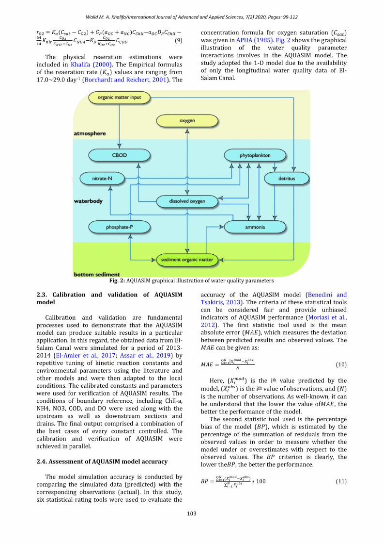
The present study concerns the west part of the Suez Canal. The study area receives a contaminated load from El-Serw and Hadous drains, which discharges domestic and agricultural wastewater. The spatial-temporal dynamics of flow was presented in Khalifa (2014). The physicochemical parameters were measured as in El-Amier et al. (2017). The selected five sampling stations along El-Salam Canal are shown in Fig. 1. The sampling station 1 lies on the Damietta branch of the River Nile (only Nile water). Therefore, Station 1 (0.00 km, 31º 23' 38" N, 31º 46' 09" E) can be considered as a reference station for all the other stations. The sampling station 2 (23.39 km, 31º 14' 07" N, 31º 50' 41" E) lies 5.0 km downstream the point of merging El-Salam Canal with El-Serw drain (18.39 km). Station 3 (59.87 km, 31º 03' 32" N, 32º 00' 37" E) lies 5.0 km downstream the merging point with Hadous drain (54.87 km). Station 4 (69.87 km, 31º 00' 48" N, 32º 04' 56" E) lies 10 km downstream the station 3. Station 5 (89.75 km, 31º 01' 07" N, 32º 18' 19" E) is located at the end of El-Salam Canal just before the siphon under Suez Canal.

Fig. 1: Sampling stations of El-Salam Canal

Mediterranean Sea

Walid M. A. Khalifa/International Journal of Advanced and Applied Sciences, 7(2) 2020, Pages: 99-112

102

2.2. Water quality modeling

The study reach is modeled using the numerical modeling approach of AQUASIM. The model was compared for the simulation of water quality on the El-Salam Canal. The calibration and validation were performed over the selected stations of El-Salam Canal. The hydraulic equations of AQUASIM were presented in Khalifa (2014). The AQUASIM applies the conservation of mass governing relation as: 𝜕𝐴𝐶

𝜕𝑡= −

𝜕(𝑄𝐶)

𝜕𝑥+

𝜕2𝐴𝐸(𝐶)

𝜕𝑥2+ 𝑟 + 𝑆𝑞𝑛 (1)

Here (A) represents the cross-sectional area of

the Canal. The first term of Eq. 1 represents the advection of concentration (𝐶) with the water flow (𝑄). The second term represents longitudinal dispersion which is estimated in Fischer et al. (1979). The third term represents the transformation processes (𝑟). The fourth term represents the lateral inflow or outflow (𝑆𝑞𝑛).

2.2.1. Modeling of water quality parameters

The parameters of water quality of El-Salam Canal are characterized by chlorophyll-a of phytoplankton compositions, NH4, NO3, COD, and DO. The chemical and biological transformation term (𝑟) in Eq. 1 for the five parameters, can be modeled with AQUASIM (Khalifa, 2000). Such parameters would be summarized in sequence. Chlorophyll-a Modeling: The kinetics of

Chlorophyll assumes the core of water quality and then affects all other parameters. The reaction term of phytoplankton (𝑟𝐶ℎ𝑙𝑙) can be expressed as a difference between the growth rate of phytoplankton and their death and respiration rates as:

𝑟𝐶ℎ𝑙𝑙 = (𝐺𝑃– 𝐷𝑃)𝐶𝐶ℎ𝑙𝑙 (2)

The growth rate (𝐺𝑃) can express the production rate of biomass as a function of the main environmental variables (temperature, light, and nutrients) as: 𝐺𝑃 = 𝐺𝑇𝐺𝐼𝐺𝑁 (3)

The temperature growth factor (𝐺𝑇) can be reported in maximum rates as (1.5~2.5 day-1) (Thomann and Mueller, 1987). AQUASIM can also present the daily depth-averaged growth rate reduction (𝐺𝐼) (Di Toro et al., 1971) using the intensity of light estimation. Finally, the growth rate reduction of ammonia concentrations (𝐺𝑁) can be considered as (Di Toro et al., 1971): 𝐺𝑁 = 𝐶𝑁𝐻4/(𝐾𝑚𝑛 + 𝐶𝑁𝐻4) (4)

A range value of the nitrogen Michaelis constant (𝐾𝑚𝑛) has been reported from 10 to 20 µg N/L

(Thomann and Mueller, 1987). The second term of Eq. 2 is related to the total biomass reduction rate as: 𝐷𝑃 = 𝐷𝑅 + 𝐷𝐷 (5)

The reported endogenous respiration rate (𝐷𝑅) varies from 0.02~0.6 day-1 (Khalifa, 2000). The death rate of phytoplankton (𝐷𝐷 ) is equal to 0.02 day-1 (Ambrose et al., 1993).

Ammonia Modeling: The reaction term of ammonia

(𝑟𝑁𝐻4) is given by: 𝑟𝑁𝐻4 = 𝑎𝑁𝐶𝑓𝑂𝑁 𝐷𝑃𝐶𝐶ℎ𝑙𝑙 − 𝑎𝑁𝐶𝑃𝑁𝐻4𝐺𝑃𝐶𝐶ℎ𝑙𝑙 −

𝐾𝑛𝑖𝑡𝐶𝑂2

𝐾𝑁𝐼𝑇+𝐶𝑂2𝐶𝑁𝐻4 (6)

The ratio of nitrogen to carbon for phytoplankton (𝑎𝑁𝐶) is reported a range of 0.1~0.35 with a mean value of 0.25 (Ambrose et al., 1993). The fraction of the cellular nitrogen recycled to the inorganic pool (𝑓𝑂𝑁 ) has been assigned at 50% (Di Toro and Matystik, 1980). The preference for ammonia uptake term (𝑃𝑁𝐻4) is reported a range of 0.22~0.83 (Ambrose et al., 1993). The nitrification rate (𝐾𝑛𝑖𝑡) is reported a range of 0.09~0.5 day-1 (Khalifa, 2000). The half-saturation constant (𝐾𝑁𝐼𝑇) is reported as 2.0 mg O2/L (Ambrose et al., 1993).

Nitrate Modeling: The reaction term of nitrate

(rNO3) is given by:

𝑟𝑁𝑂3 = 𝐾𝑛𝑖𝑡𝐶𝑂2

𝐾𝑁𝐼𝑇+𝐶𝑂2𝐶𝑁𝐻4 − 𝑎𝑁𝐶(1 − 𝑃𝑁𝐻4)𝐺𝑃𝐶𝐶ℎ𝑙𝑙 −

𝐾𝑑𝑒𝑛𝐾𝑁𝑂3

𝐾𝑁𝑂3+𝐶𝑂2𝐶𝑁𝑂3 (7)

A range value of denitrification rate (𝐾𝑑𝑒𝑛) has been reported as 0.1~0.5 day-1 (Thomann and Mueller, 1987). In addition, the denitrification rate has been reported as 0.09 day-1 and Michaelis constant for denitrification (𝐾𝑁𝑂3) as 0.1 mg O2/L for (Ambrose et al., 1993): Chemical Oxygen Demand (COD) Modeling: The

rate of oxidation of COD is the controlling kinetic reaction (𝑟𝐶𝑂𝐷) as:

𝑟𝐶𝑂𝐷 = 𝑎𝑂𝐶𝐷𝐷𝐶𝐶ℎ𝑙𝑙−𝐾𝐷𝐶𝑂2

𝐾𝑂2+𝐶𝑂2𝐶𝐶𝑂𝐷 (8)

The ratio of oxygen to carbon for phytoplankton (𝑎𝑂𝐶 ) has been reported as an approximation value of 2.7 and the deoxygenation rate (𝐾𝐷) of about 0.1~0.5 day-1 (Thomann and Mueller, 1987). A range of (𝐾𝐷) has been reported as 0.16~0.21 day-1 and Michaelis constant of oxidation (𝐾𝑂2) as 0.5 mg O2/L (Ambrose et al., 1993).

Dissolved Oxygen (DO) Modeling: The oxygen

balance is characterized by intense production-respiration-nitrification-deoxygenation processes. According to Eq. 1, it can be modeled the oxygen balance with these processes to formulate their kinetics explicitly using Eq. 9:

Walid M. A. Khalifa/International Journal of Advanced and Applied Sciences, 7(2) 2020, Pages: 99-112

103

𝑟𝑂2 = 𝐾𝑎(𝐶𝑠𝑎𝑡 − 𝐶𝑂2) + 𝐺𝑃(𝑎𝑂𝐶 + 𝑎𝑁𝐶)𝐶𝐶ℎ𝑙𝑙−𝑎𝑂𝐶𝐷𝑅𝐶𝐶ℎ𝑙𝑙 −64

14𝐾𝑛𝑖𝑡

𝐶𝑂2

𝐾𝑁𝐼𝑇+𝐶𝑂2𝐶𝑁𝐻4−𝐾𝐷

𝐶𝑂2

𝐾𝑂2+𝐶𝑂2𝐶𝐶𝑂𝐷 (9)

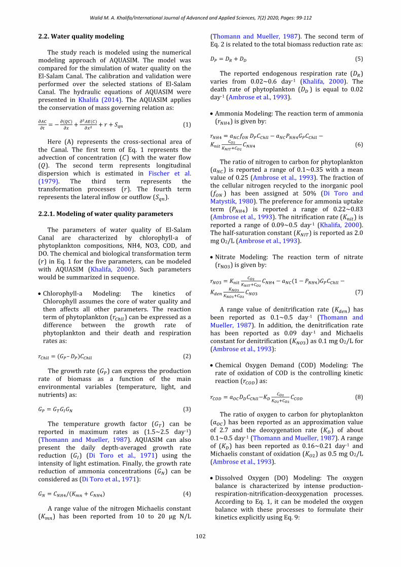
The physical reaeration estimations were included in Khalifa (2000). The Empirical formulas of the reaeration rate (𝐾𝑎) values are ranging from 17.0~29.0 day-1 (Borchardt and Reichert, 2001). The

concentration formula for oxygen saturation (𝐶𝑠𝑎𝑡) was given in APHA (1985). Fig. 2 shows the graphical illustration of the water quality parameter interactions involves in the AQUASIM model. The study adopted the 1-D model due to the availability of only the longitudinal water quality data of El-Salam Canal.

Fig. 2: AQUASIM graphical illustration of water quality parameters

2.3. Calibration and validation of AQUASIM model

Calibration and validation are fundamental processes used to demonstrate that the AQUASIM model can produce suitable results in a particular application. In this regard, the obtained data from El-Salam Canal were simulated for a period of 2013-2014 (El-Amier et al., 2017; Assar et al., 2019) by repetitive tuning of kinetic reaction constants and environmental parameters using the literature and other models and were then adapted to the local conditions. The calibrated constants and parameters were used for verification of AQUASIM results. The conditions of boundary reference, including Chll-a, NH4, NO3, COD, and DO were used along with the upstream as well as downstream sections and drains. The final output comprised a combination of the best cases of every constant controlled. The calibration and verification of AQUASIM were achieved in parallel.

2.4. Assessment of AQUASIM model accuracy

The model simulation accuracy is conducted by comparing the simulated data (predicted) with the corresponding observations (actual). In this study, six statistical rating tools were used to evaluate the

accuracy of the AQUASIM model (Benedini and Tsakiris, 2013). The criteria of these statistical tools can be considered fair and provide unbiased indicators of AQUASIM performance (Moriasi et al., 2012). The first statistic tool used is the mean absolute error (𝑀𝐴𝐸), which measures the deviation between predicted results and observed values. The 𝑀𝐴𝐸 can be given as:

𝑀𝐴𝐸 =∑ |𝑋𝑖

𝑚𝑜𝑑−𝑋𝑖𝑜𝑏𝑠|𝑁

𝑖=1

𝑁 (10)

Here, (𝑋𝑖𝑚𝑜𝑑) is the ith value predicted by the

model, (𝑋𝑖𝑜𝑏𝑠) is the ith value of observations, and (𝑁)

is the number of observations. As well-known, it can be understood that the lower the value of𝑀𝐴𝐸, the better the performance of the model.

The second statistic tool used is the percentage bias of the model (𝐵𝑃), which is estimated by the percentage of the summation of residuals from the observed values in order to measure whether the model under or overestimates with respect to the observed values. The 𝐵𝑃 criterion is clearly, the lower the𝐵𝑃, the better the performance.

𝐵𝑃 =∑ (𝑋𝑖

𝑚𝑜𝑑−𝑋𝑖𝑜𝑏𝑠)𝑁

𝑖=1

∑ 𝑋𝑖𝑜𝑏𝑠𝑁

𝑖=1

∗ 100 (11)

Walid M. A. Khalifa/International Journal of Advanced and Applied Sciences, 7(2) 2020, Pages: 99-112

104

The performance evaluation criteria have been reported that water quality models have been adopted as very good for (𝐵𝑃<15%), good for (15%𝐵𝑃25%), and fair for (25%𝐵𝑃35%). Some concerns of 𝐵𝑃 criterion can deceive the model performance rating where PB can close to zero however the model simulation is poor. So, it is recommended to use 𝐵𝑃 with other statistical analyses to determine the model performance (Moriasi et al., 2012).

The third statistic tool used is the root mean square error (𝑅𝑀𝑆𝐸), which represents the standard deviations of observed and predicted values. The 𝑅𝑀𝑆𝐸 units are the same as the units of the model predictions and observations. The model performance indicates well when values of 𝑅𝑀𝑆𝐸 are near to zero (Moriasi et al., 2012).

𝑅𝑀𝑆𝐸 = [∑ (𝑋𝑖

𝑚𝑜𝑑−𝑋𝑖𝑜𝑏𝑠)2𝑁

𝑖=1

𝑁]

1/2

(12)

The 𝑅𝑀𝑆𝐸 has not been suggested a good indicator to evaluate the model performance and maybe a misleading indicator of average error, and the 𝑀𝐴𝐸 has been suggested better criteria for that purpose (Willmott and Matsuura, 2005). While some concerns over using 𝑅𝑀𝑆𝐸 are valid, the 𝑅𝑀𝑆𝐸 is more suitable to represent model performance than the 𝑀𝐴𝐸 (Chai and Draxler, 2014).

The fourth statistic tool used is the relative root mean square error (𝑅𝑅𝑀𝑆𝐸) which is defined as:

𝑅𝑅𝑀𝑆𝐸 =1

𝑋𝑜𝑏𝑠̅̅ ̅̅ ̅̅ ̅ [∑ (𝑋𝑖

𝑚𝑜𝑑−𝑋𝑖𝑜𝑏𝑠)2𝑁

𝑖=1

𝑁]

1/2

(13)

Here, (𝑋𝑜𝑏𝑠̅̅ ̅̅ ̅̅ ) is the mean of observed values. 𝑅𝑅𝑀𝑆𝐸 is the same as𝑅𝑀𝑆𝐸, but normalized by the mean value of (𝑋𝑜𝑏𝑠), giving an indication of the scatter in relation to mean value. As the error lessens, the model prediction accuracy rises (Benedini and Tsakiris, 2013).

The fifth statistic tool used is the coefficient of determination (𝑅2), which evaluates the relative deviation of predicted results from the observed data obtained by the model. The (𝑅2) can be expressed by squaring the Pearson correlation coefficient (PCC) equation as:

𝑅2 = (∑ (𝑋𝑖

𝑜𝑏𝑠−𝑋𝑜𝑏𝑠̅̅ ̅̅ ̅̅ ̅)(𝑋𝑖𝑚𝑜𝑑−𝑋𝑚𝑜𝑑̅̅ ̅̅ ̅̅ ̅̅ )𝑁

𝑖=1

√[∑ (𝑋𝑖𝑜𝑏𝑠−𝑋𝑜𝑏𝑠̅̅ ̅̅ ̅̅ ̅)2𝑁

𝑖=1 ]√[∑ (𝑋𝑖𝑚𝑜𝑑−𝑋𝑚𝑜𝑑̅̅ ̅̅ ̅̅ ̅̅ )2𝑁

𝑖=1 ]

)

2

(14)

If (𝑅2) approaches 1, a strong positive relationship between the observed and predicted can be attained. The reported performance evaluation criteria for water quality models have been adopted as very good for (𝑅2>0.85), good for (0.75𝑅20.85), satisfactory for (0.7<𝑅2<0.75), and poor for (𝑅20.7) (Moriasi et al., 2012).

The sixth statistic tool used is Nash–Sutcliffe’s model efficiency (𝑁𝑆𝐸), which measures the ratio of the model deviation from the true (observed) data as:

𝑁𝑆𝐸 = 1 −∑ (𝑋𝑖

𝑚𝑜𝑑−𝑋𝑖𝑜𝑏𝑠)2𝑁

𝑖=1

∑ (𝑋𝑖𝑜𝑏𝑠−𝑋𝑜𝑏𝑠̅̅ ̅̅ ̅̅ ̅)2𝑁

𝑖=1

(15)

The value of 𝑁𝑆𝐸 varies from -α to 1.0, with 1.0 being the optimal value. Values between 0 and 1 are generally considered acceptable, whereas negative values imply unacceptable model performance (Benedini and Tsakiris, 2013).

In general, the acceptable water quality model simulation has been reported as (𝑅2 0.8, 𝑁𝑆𝐸 0.7, and 𝐵𝑃15%) (Moriasi et al., 2012). In the meanwhile, the good water quality model performance is considered (𝐵𝑃<30%) for nutrients and (𝐵𝑃<50%) for phytoplankton (Moriasi et al., 2012).

2.5. Water quality index (WQI) development

WQI is a comparative single number that reflects the combined effects of several water quality parameters on the general quality of a certain location and time. This manner is easier to use and understand the characteristics of water quality parameters. As a whole, several institutions have developed 𝑊𝑄𝐼 based on their priorities, institutional capacities, and levels of technology. There are several 𝑊𝑄𝐼 methods, based on the weighted arithmetic index. The main weighted arithmetic means method for deriving 𝑊𝑄𝐼 is the quality rating method (Wu et al., 2018; Bora and Goswami, 2017; Shah and Joshi, 2017). The 𝑊𝑄𝐼 was deduced from the quality rating method (Horton, 1965) as:

𝑊𝑄𝐼 =∑𝑞𝑛𝑊𝑛

∑𝑊𝑛 (16)

Here, (𝑞𝑛) is the rating of the quality of nth water quality parameter and (𝑊𝑛) is the unit weight of the nth water quality parameter. The rating of quality (𝑞𝑛) is calculated using the expression given in Brown et al. (1972) as:

𝑞𝑛 = [(𝑉𝑛−𝑉𝑖𝑑)

(𝑆𝑛−𝑉𝑖𝑑)] ∗ 100 (17)

Here, (𝑉𝑛) is the estimated value of nth water quality parameter at a given sample location, (𝑆𝑛) is the standard allowable value of nth water quality parameter, and (𝑉𝑖𝑑) is the ideal value for the nth water quality parameter in pure water. The unit weight (𝑊𝑛) is calculated as:

𝑊𝑛 =𝑘

𝑆𝑛 (18)

Here, (𝑘) is the proportionality constant and is calculated as:

𝑘 =1

∑(1

𝑆𝑛) (19)

The status of water corresponding to the 𝑊𝑄𝐼 is categorized into five types which are given in Srinivas et al. (2016). The study has used basic

Walid M. A. Khalifa/International Journal of Advanced and Applied Sciences, 7(2) 2020, Pages: 99-112

105

sixteen physiochemical parameters which were presented in El-Amier et al. (2017).

3. Results and discussion

The present study includes three major objectives. The first one is the simulation of water quality of El-Salam Canal for the parameters: Chll-a, NH4, NO3, COD, and DO using the computer modeling program AQUASIM. The second target is to evaluate El-Salam Canal’s water quality using the water quality index. The third objective is to study the effect of flow on the spatial profile of El-Salam Canal’s water quality. In the subsequent articles, it can be possible to detail these targets.

3.1. AQUASIM model calibration and validation

The performance of the AQUASIM model has been evaluated based on the simulated and observed results of Chll-a, NH4, NO3, COD, and DO at their corresponding monitoring stations of El-Salam Canal. The AQUASIM hydraulic model calibration and the water level profile of the El-Salam Canal were early presented in Khalifa (2014). The basic water quality modeling capability of AQUASIM to predict the mean concentration field may be the inflow-outflow boundaries.

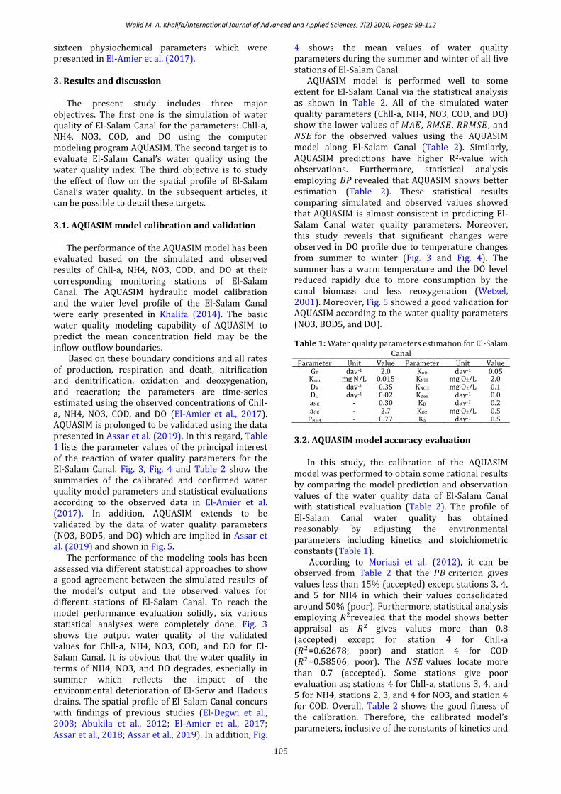
Based on these boundary conditions and all rates of production, respiration and death, nitrification and denitrification, oxidation and deoxygenation, and reaeration; the parameters are time-series estimated using the observed concentrations of Chll-a, NH4, NO3, COD, and DO (El-Amier et al., 2017). AQUASIM is prolonged to be validated using the data presented in Assar et al. (2019). In this regard, Table 1 lists the parameter values of the principal interest of the reaction of water quality parameters for the El-Salam Canal. Fig. 3, Fig. 4 and Table 2 show the summaries of the calibrated and confirmed water quality model parameters and statistical evaluations according to the observed data in El-Amier et al. (2017). In addition, AQUASIM extends to be validated by the data of water quality parameters (NO3, BOD5, and DO) which are implied in Assar et al. (2019) and shown in Fig. 5.

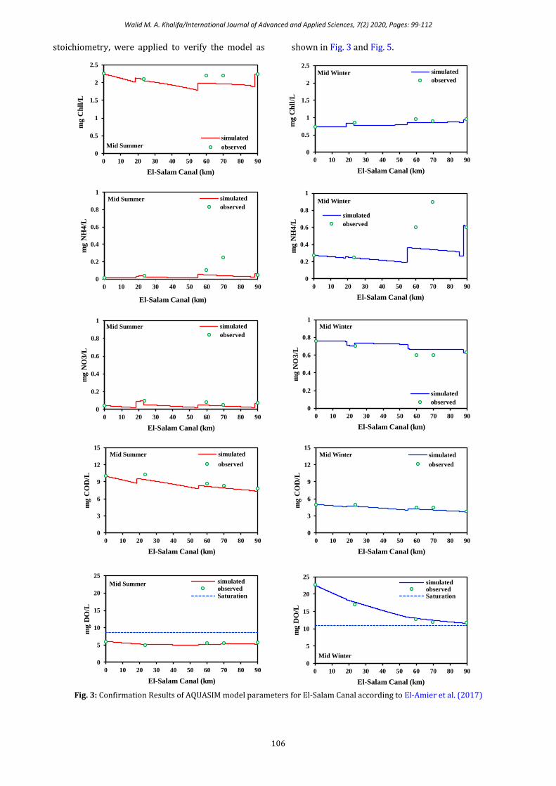
The performance of the modeling tools has been assessed via different statistical approaches to show a good agreement between the simulated results of the model’s output and the observed values for different stations of El-Salam Canal. To reach the model performance evaluation solidly, six various statistical analyses were completely done. Fig. 3 shows the output water quality of the validated values for Chll-a, NH4, NO3, COD, and DO for El-Salam Canal. It is obvious that the water quality in terms of NH4, NO3, and DO degrades, especially in summer which reflects the impact of the environmental deterioration of El-Serw and Hadous drains. The spatial profile of El-Salam Canal concurs with findings of previous studies (El-Degwi et al., 2003; Abukila et al., 2012; El-Amier et al., 2017; Assar et al., 2018; Assar et al., 2019). In addition, Fig.

4 shows the mean values of water quality parameters during the summer and winter of all five stations of El-Salam Canal.

AQUASIM model is performed well to some extent for El-Salam Canal via the statistical analysis as shown in Table 2. All of the simulated water quality parameters (Chll-a, NH4, NO3, COD, and DO) show the lower values of 𝑀𝐴𝐸, 𝑅𝑀𝑆𝐸, 𝑅𝑅𝑀𝑆𝐸, and 𝑁𝑆𝐸 for the observed values using the AQUASIM model along El-Salam Canal (Table 2). Similarly, AQUASIM predictions have higher R2-value with observations. Furthermore, statistical analysis employing 𝐵𝑃 revealed that AQUASIM shows better estimation (Table 2). These statistical results comparing simulated and observed values showed that AQUASIM is almost consistent in predicting El-Salam Canal water quality parameters. Moreover, this study reveals that significant changes were observed in DO profile due to temperature changes from summer to winter (Fig. 3 and Fig. 4). The summer has a warm temperature and the DO level reduced rapidly due to more consumption by the canal biomass and less reoxygenation (Wetzel, 2001). Moreover, Fig. 5 showed a good validation for AQUASIM according to the water quality parameters (NO3, BOD5, and DO).

Table 1: Water quality parameters estimation for El-Salam Canal

Parameter Unit Value Parameter Unit Value GT day-1 2.0 Knit day-1 0.05

Kmn mg N/L 0.015 KNIT mg O2/L 2.0 DR day-1 0.35 KNO3 mg O2/L 0.1 DD day-1 0.02 Kden day-1 0.0 aNC - 0.30 KD day-1 0.2 aOC - 2.7 KO2 mg O2/L 0.5

PNH4 - 0.77 Ka day-1 0.5

3.2. AQUASIM model accuracy evaluation

In this study, the calibration of the AQUASIM model was performed to obtain some rational results by comparing the model prediction and observation values of the water quality data of El-Salam Canal with statistical evaluation (Table 2). The profile of El-Salam Canal water quality has obtained reasonably by adjusting the environmental parameters including kinetics and stoichiometric constants (Table 1).

According to Moriasi et al. (2012), it can be observed from Table 2 that the 𝑃𝐵 criterion gives values less than 15% (accepted) except stations 3, 4, and 5 for NH4 in which their values consolidated around 50% (poor). Furthermore, statistical analysis employing 𝑅2revealed that the model shows better appraisal as 𝑅2 gives values more than 0.8 (accepted) except for station 4 for Chll-a (𝑅2=0.62678; poor) and station 4 for COD (𝑅2=0.58506; poor). The 𝑁𝑆𝐸 values locate more than 0.7 (accepted). Some stations give poor evaluation as; stations 4 for Chll-a, stations 3, 4, and 5 for NH4, stations 2, 3, and 4 for NO3, and station 4 for COD. Overall, Table 2 shows the good fitness of the calibration. Therefore, the calibrated model’s parameters, inclusive of the constants of kinetics and

Walid M. A. Khalifa/International Journal of Advanced and Applied Sciences, 7(2) 2020, Pages: 99-112

106

stoichiometry, were applied to verify the model as shown in Fig. 3 and Fig. 5.

Fig. 3: Confirmation Results of AQUASIM model parameters for El-Salam Canal according to El-Amier et al. (2017)

0

0.5

1

1.5

2

2.5

0 10 20 30 40 50 60 70 80 90

mg

Ch

ll/L

El-Salam Canal (km)

Mid Summer

simulated

observed0

0.5

1

1.5

2

2.5

0 10 20 30 40 50 60 70 80 90

mg

Ch

ll/L

El-Salam Canal (km)

Mid Winter simulated

observed

0

0.2

0.4

0.6

0.8

1

0 10 20 30 40 50 60 70 80 90

mg

NH

4/L

El-Salam Canal (km)

Mid Summer simulated

observed

0

0.2

0.4

0.6

0.8

1

0 10 20 30 40 50 60 70 80 90m

g N

H4

/LEl-Salam Canal (km)

Mid Winter

simulated

observed

0

0.2

0.4

0.6

0.8

1

0 10 20 30 40 50 60 70 80 90

mg

NO

3/L

El-Salam Canal (km)

Mid Summer simulated

observed

0

0.2

0.4

0.6

0.8

1

0 10 20 30 40 50 60 70 80 90

mg

NO

3/L

El-Salam Canal (km)

Mid Winter

simulated

observed

0

3

6

9

12

15

0 10 20 30 40 50 60 70 80 90

mg

CO

D/L

El-Salam Canal (km)

Mid Summer simulated

observed

0

3

6

9

12

15

0 10 20 30 40 50 60 70 80 90

mg

CO

D/L

El-Salam Canal (km)

Mid Winter simulated

observed

0

5

10

15

20

25

0 10 20 30 40 50 60 70 80 90

mg

DO

/L

El-Salam Canal (km)

Mid Summer simulated

observed

Saturation

0

5

10

15

20

25

0 10 20 30 40 50 60 70 80 90

mg

DO

/L

El-Salam Canal (km)

Mid Winter

simulatedobservedSaturation

Walid M. A. Khalifa/International Journal of Advanced and Applied Sciences, 7(2) 2020, Pages: 99-112

107

Table 2: Statistical evaluation of calibrated and validation results for predicted and observed Parameter Location MAE BP% RMSE RRMSE R2 NSE

Chll-a

Station 1 0.00026 0.02603 0.00062 0.00063 1.00000 1.00000

Station 2 0.05752 5.47962 0.08419 0.08021 0.98403 0.96891

Station 3 0.05814 5.62298 0.09651 0.09334 0.97592 0.95829

Station 4 0.15591 13.78702 0.37770 0.33400 0.62678 0.55013

Station 5 0.08451 8.19838 0.13451 0.13049 0.98708 0.93021

NH4

Station 1 0.00020 0.13481 0.00023 0.00158 1.00000 1.00000

Station 2 0.01452 9.64065 0.01875 0.12445 0.99694 0.98212

Station 3 0.16193 45.39707 0.30526 0.85579 0.92184 0.58901

Station 4 0.26552 58.96171 0.28063 0.62318 0.86498 -0.29928

Station 5 0.15439 50.98510 0.27376 0.90408 0.87885 0.56645

NO3

Station 1 0.00007 0.01636 0.00030 0.00074 1.00000 1.00000

Station 2 0.03193 -9.21629 0.14117 0.40754 0.85267 0.51523

Station 3 0.03954 -12.8538 0.12455 0.40491 0.86556 0.50139

Station 4 0.04547 -15.2052 0.11407 0.38148 0.88644 0.66543

Station 5 0.04424 -14.6081 0.10044 0.33163 0.94322 0.78407

COD

Station 1 0.01180 0.13277 0.01411 0.00159 1.00000 0.99998

Station 2 0.56667 6.57095 1.01914 0.11818 0.91801 0.87774

Station 3 0.75126 9.80090 1.21720 0.15880 0.90072 0.80602

Station 4 0.08018 -1.23491 1.33403 0.20546 0.58506 0.25652

Station 5 0.23625 3.81386 0.49615 0.08010 0.95944 0.90712

DO

Station 1 0.02033 0.18227 0.02614 0.00234 1.00000 0.99997

Station 2 0.11009 1.13446 0.85526 0.08822 0.94290 0.94161

Station 3 0.16910 2.03189 0.49676 0.05970 0.96857 0.96223

Station 4 0.20386 2.38767 0.71312 0.08374 0.90645 0.80528

Station 5 0.18473 2.38319 0.57124 0.07373 0.92288 0.91079

Fig. 4: Mean values of water quality parameters during summer and winter along El-Salam Canal according to El-Amier et

al. (2017)

0.0

0.4

0.8

1.2

1.6

2.0

Station 1 Station 2 Station 3 Station 4 Station 5

Ch

ll (

mg

/L)

simulated (S) Observed (S) simulated (W) Observed (W)

0.0

0.2

0.4

0.6

0.8

1.0

Station 1 Station 2 Station 3 Station 4 Station 5

NH

4 (

mg

/L)

simulated (S) Observed (S) simulated (W) Observed (W)

0.0

0.2

0.4

0.6

0.8

1.0

Station 1 Station 2 Station 3 Station 4 Station 5

NO

3 (

mg

/L)

simulated (S) Observed (S) simulated (W) Observed (W)

0

3

6

9

12

15

Station 1 Station 2 Station 3 Station 4 Station 5

CO

D (

mg

/L)

simulated (S) Observed (S) simulated (W) Observed (W)

0

3

6

9

12

15

Station 1 Station 2 Station 3 Station 4 Station 5

DO

(m

g/L

)

simulated (S) Observed (S) simulated (W) Observed (W)

Walid M. A. Khalifa/International Journal of Advanced and Applied Sciences, 7(2) 2020, Pages: 99-112

108

Fig. 5: Confirmation Results of water quality model parameters for El-Salam Canal according to Assar et al. (2019)

3.3. Water quality index (WQI) assessment

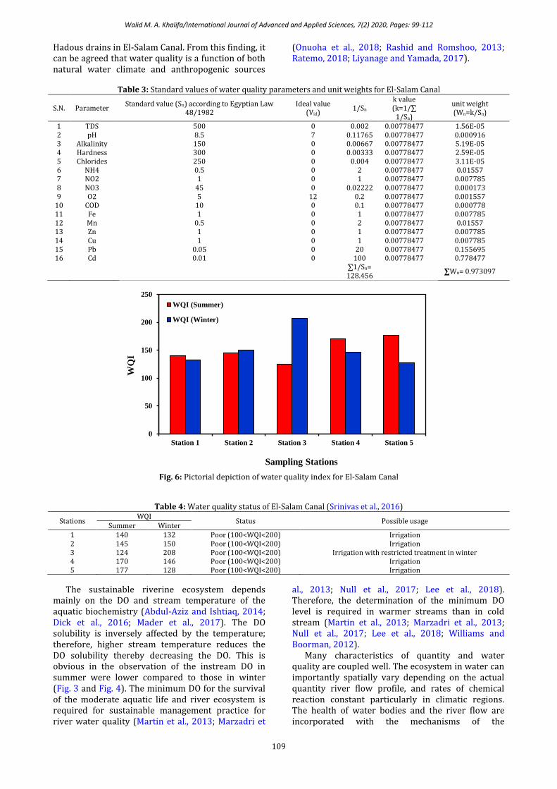
𝑊𝑄𝐼 is produced by using the physicochemical variables measured for El-Salam Canal as presented in El-Amier et al. (2017). Sixteen parameters have been selected as shown in Table 3. The standard values (𝑆𝑛) are in mg/L except p forH, and can be estimated according to Egyptian Law (48/1982) in 1995 and its revision (48/1982) in 1999. Fig. 6 shows the pictorial depiction of the water quality index for El-Salam Canal. In this regard, it can be possible to summarize the water quality status for El-Salam Canal as shown in Table 4. It is clearly noticed that the water quality in station 3 (near Hadous drain), was affected by agricultural and domestic uses especially in winter due to the closure system (Abu-Zeid, 1995). Therefore, minimizing these pollution sources should be the priority to improve the water quality around this area.

3.4. Interrelationship of spatial scale among water quality parameters

Fig. 7 shows the interrelationship of spatial scale among the quantity of El-Salam Canal flow profile and the DO concentrations. Usually, the DO concentrations are improved by a high rate of fresh-water flow. However, exceptions of different climatic zone occur since the concentration of DO, COD, and nitrogen also depends on the different reaction rates. Fig. 7 shows that the concentration of DO declines with respect to the flow profile as a tropical zone of north Egypt (Khalifa, 2014). This study shows that the DO concentration increases in winter, while DO concentration declines clearly in summer (Fig. 3 and Fig. 4). The greater possibility of a high reoxygenation rate is also observed in winter than in summer (Fig. 3 and Fig. 4). Overall, the COD profile trend is increasing with increasing phytoplankton in summer which is due to the addition of El-Serw and

0

0.3

0.6

0.9

1.2

1.5

1-S

ep-1

3

1-O

ct-1

3

1-N

ov-1

3

1-D

ec-

13

1-J

an

-14

1-F

eb

-14

1-M

ar-

14

1-A

pr-

14

1-M

ay

-14

1-J

un

-14

1-J

ul-

14

1-A

ug-1

4

1-S

ep

-14

NO3 at 4 km DS of El-Serw Drain

simulated

observedm

gN

O3

/L

0

0.3

0.6

0.9

1.2

1.5

1-S

ep

-13

1-O

ct-1

3

1-N

ov-1

3

1-D

ec-

13

1-J

an

-14

1-F

eb

-14

1-M

ar-1

4

1-A

pr-

14

1-M

ay-1

4

1-J

un

-14

1-J

ul-

14

1-A

ug-1

4

1-S

ep

-14

NO3 at 1 km US of Hadous Drain

simulated

observed

mg

NO

3/L

0

4

8

12

16

20

1-S

ep

-13

1-O

ct-1

3

1-N

ov

-13

1-D

ec-

13

1-J

an

-14

1-F

eb

-14

1-M

ar-1

4

1-A

pr-

14

1-M

ay

-14

1-J

un

-14

1-J

ul-

14

1-A

ug

-14

1-S

ep

-14

Biomass at 4 km DS of El-Serw Drain

simulated

observed

mg

BO

D5

/L

0

4

8

12

16

20

1-S

ep

-13

1-O

ct-1

3

1-N

ov

-13

1-D

ec-

13

1-J

an

-14

1-F

eb

-14

1-M

ar-1

4

1-A

pr-

14

1-M

ay

-14

1-J

un

-14

1-J

ul-

14

1-A

ug

-14

1-S

ep

-14

Biomass at 1 km US of Hadous Drain

simulated

observed

mg

BO

D5

/L

0

5

10

15

20

25

1-S

ep

-13

1-O

ct-1

3

1-N

ov

-13

1-D

ec-

13

1-J

an

-14

1-F

eb

-14

1-M

ar-1

4

1-A

pr-

14

1-M

ay

-14

1-J

un

-14

1-J

ul-

14

1-A

ug

-14

1-S

ep

-14

DO at 4 km DS of El-Serw Drain

simulated

observed

saturation

mg

DO

/L

0

5

10

15

20

25

1-S

ep

-13

1-O

ct-1

3

1-N

ov

-13

1-D

ec-

13

1-J

an

-14

1-F

eb

-14

1-M

ar-1

4

1-A

pr-

14

1-M

ay

-14

1-J

un

-14

1-J

ul-

14

1-A

ug

-14

1-S

ep

-14

DO at 1 km US of Hadous Drain

simulated

observed

saturation

mg

DO

/L

Walid M. A. Khalifa/International Journal of Advanced and Applied Sciences, 7(2) 2020, Pages: 99-112

109

Hadous drains in El-Salam Canal. From this finding, it can be agreed that water quality is a function of both natural water climate and anthropogenic sources

(Onuoha et al., 2018; Rashid and Romshoo, 2013; Ratemo, 2018; Liyanage and Yamada, 2017).

Table 3: Standard values of water quality parameters and unit weights for El-Salam Canal

S.N. Parameter Standard value (Sn) according to Egyptian Law

48/1982 Ideal value

(Vid) 1/Sn

k value (k=1/∑

1/Sn)

unit weight (Wn=k/Sn)

1 TDS 500 0 0.002 0.00778477 1.56E-05 2 pH 8.5 7 0.11765 0.00778477 0.000916 3 Alkalinity 150 0 0.00667 0.00778477 5.19E-05 4 Hardness 300 0 0.00333 0.00778477 2.59E-05 5 Chlorides 250 0 0.004 0.00778477 3.11E-05 6 NH4 0.5 0 2 0.00778477 0.01557 7 NO2 1 0 1 0.00778477 0.007785 8 NO3 45 0 0.02222 0.00778477 0.000173 9 O2 5 12 0.2 0.00778477 0.001557

10 COD 10 0 0.1 0.00778477 0.000778 11 Fe 1 0 1 0.00778477 0.007785 12 Mn 0.5 0 2 0.00778477 0.01557 13 Zn 1 0 1 0.00778477 0.007785 14 Cu 1 0 1 0.00778477 0.007785 15 Pb 0.05 0 20 0.00778477 0.155695 16 Cd 0.01 0 100 0.00778477 0.778477

∑1/Sn= 128.456

∑Wn= 0.973097

Fig. 6: Pictorial depiction of water quality index for El-Salam Canal

Table 4: Water quality status of El-Salam Canal (Srinivas et al., 2016)

Stations WQI

Status Possible usage Summer Winter

1 140 132 Poor (100<WQI<200) Irrigation 2 145 150 Poor (100<WQI<200) Irrigation 3 124 208 Poor (100<WQI<200) Irrigation with restricted treatment in winter 4 170 146 Poor (100<WQI<200) Irrigation 5 177 128 Poor (100<WQI<200) Irrigation

The sustainable riverine ecosystem depends mainly on the DO and stream temperature of the aquatic biochemistry (Abdul-Aziz and Ishtiaq, 2014; Dick et al., 2016; Mader et al., 2017). The DO solubility is inversely affected by the temperature; therefore, higher stream temperature reduces the DO solubility thereby decreasing the DO. This is obvious in the observation of the instream DO in summer were lower compared to those in winter (Fig. 3 and Fig. 4). The minimum DO for the survival of the moderate aquatic life and river ecosystem is required for sustainable management practice for river water quality (Martin et al., 2013; Marzadri et

al., 2013; Null et al., 2017; Lee et al., 2018). Therefore, the determination of the minimum DO level is required in warmer streams than in cold stream (Martin et al., 2013; Marzadri et al., 2013; Null et al., 2017; Lee et al., 2018; Williams and Boorman, 2012).

Many characteristics of quantity and water quality are coupled well. The ecosystem in water can importantly spatially vary depending on the actual quantity river flow profile, and rates of chemical reaction constant particularly in climatic regions. The health of water bodies and the river flow are incorporated with the mechanisms of the

0

50

100

150

200

250

Station 1 Station 2 Station 3 Station 4 Station 5

WQ

I

Sampling Stations

WQI (Summer)

WQI (Winter)

Walid M. A. Khalifa/International Journal of Advanced and Applied Sciences, 7(2) 2020, Pages: 99-112

110

environment. The sustainability of the water environment is the objective of water quality conservation approaches such as the quantity and quality required to maintain water bodies at a safe level (Chen et al., 2013). In addition, most researches are concerned with the flow quantity to conserve the ecological health of a river (Scherman et al., 2003), which influence the water environment sustainability.

Fig. 7: DO concentration with respect to flow profile of El-

Salam Canal

4. Conclusions

This study is approached for three main objectives. Firstly, the AQUASIM model is used to evaluate the spatially and temporal profiles of water quality of five parameters: Chlorophyll, ammonia, nitrate, chemical oxygen demand, and dissolved oxygen through El-Salam Canal in Egypt. The performance of AQUASIM predictions are assessed by applying various statistical rating tools such as 𝑀𝐴𝐸, 𝐵𝑃, 𝑅𝑀𝑆𝐸, 𝑅𝑅𝑀𝑆𝐸, 𝑅2, and 𝑁𝑆𝐸. The simulation results showed a good agreement for almost all of the water quality parameters. The second target is to evaluate the water quality of El-Salam Canal using the water quality index (𝑊𝑄𝐼) for selected sixteen parameters. The 𝑊𝑄𝐼 showed that the water quality of the EL-Salam Canal was affected by anthropogenic activities of agricultural and domestic uses especially near the Hadous drain. Therefore, it is important for minimizing these pollution sources to maintain or improve water quality around this area. This leads to assist the process of decision-making for the water quality management in EL-Salam Canal. The third target of this study shows a decline in DO of El-Salam Canal with respect to the flow profile as a tropical zone of northern Egypt.

The cold conditions as in winter show an increase in DO, expressing high reoxygenation rates while the warm conditions as in summer show a decrease in DO, demonstration low reoxygenation and high biomass deoxygenation rates. The results of the present study are convenient in the observing and control of different nutrients loads of El-Salam Canal water quality. The outcomes acquired in this study will facilitate the development of a policy for the operational enhancement of sustainable water quality in El-Salam Canal.

Compliance with ethical standards

Conflict of interest

The authors declare that they have no conflict of interest.

References

Abdul-Aziz OI and Ishtiaq KS (2014). Robust empirical modeling of dissolved oxygen in small rivers and streams: Scaling by a single reference observation. Journal of Hydrology, 511: 648-657. https://doi.org/10.1016/j.jhydrol.2014.02.022

Abukila AF, El Kholy RMS, and Kandil MI (2012). Assessment of water resources management and quality of El Salam Canal, Egypt. International Journal of Environmental Engineering, 4(1/2): 34-54. https://doi.org/10.1504/IJEE.2012.048101

Abu-Zeid M (1995). Major policies and programs for irrigation drainage and water resources development in Egypt. In: Hakim AT (Ed.), Egyptian Agriculture Profile: 33-49. CIHEAM IAM Montpellier, Montpellier, France.

Ahmed HA, Mosalem TM, Abd-El Hady ES, and Abdel-Fattah AS (2018). Assessment of water quality of El-Salam Canal west of Suez Canal, Egypt. Journal of Soil Science and Agricultural Engineering, 9(1): 43-46. https://doi.org/10.21608/jssae.2018.35540

Ambrose RB, Wool TA, and Martin JL (1993). The water quality analysis simulation program, WASP5, Part A: Model documentation. Environmental Research Laboratory, US Environmental Protection Agency, Athens, USA.

Ambrose RBJ, Wool TA, Martin JL, Shanahan P, and Alam MM (2001). WASP–Water quality analysis simulation program, Version 5.2-MDEP, model documentation. Environmental Research Laboratory and AScI Corporation, Athens, USA.

APHA (1985). Standard methods for the examination of water and waste water. 16th Edition, American Public Health Association, Washington, USA.

Assar W, Allam A, and Tawfik A (2018). Assessment and data assimilation of agricultural drainage water for reuse in irrigation purposes. In the Advances in Science and Engineering Technology International Conferences, IEEE, Abu Dhabi, UAE: 1-5. https://doi.org/10.1109/ICASET.2018.8376764

Assar W, Ibrahim MG, Mahmod W, and Fujii M (2019). Assessing the agricultural drainage water with water quality indices in the El-Salam Canal mega project, Egypt. Water, 11(5): 1013. https://doi.org/10.3390/w11051013

Benedini M and Tsakiris G (2013). Water quality modelling for rivers and streams. Springer Science and Business Media, Berlin, Germany. https://doi.org/10.1007/978-94-007-5509-3

Bora M and Goswami DC (2017). Water quality assessment in terms of water quality index (WQI): Case study of the Kolong River, Assam, India. Applied Water Science, 7(6): 3125-3135. https://doi.org/10.1007/s13201-016-0451-y

Borchardt D and Reichert P (2001). River water quality model no. 1 (RWQM1): Case study. I. Compartmentalisation approach applied to oxygen balances in the River Lahn (Germany). Water Science and Technology, 43(5): 41-49. https://doi.org/10.2166/wst.2001.0247

Brhane GK (2016). Irrigation water quality index and GIS approach based groundwater quality assessment and evaluation for irrigation purpose in Ganta Afshum selected Kebeles, Northern Ethiopia. International Journal of Emerging Trends in Science and Technology, 3(09): 4624-4636. https://doi.org/10.18535/ijetst/v3i09.10

y = -0.0639x + 12.941R² = 0.2192

0

5

10

15

20

25

0 25 50 75 100 125

DO

(m

g/

L)

Flow Profile (m3/s)

Walid M. A. Khalifa/International Journal of Advanced and Applied Sciences, 7(2) 2020, Pages: 99-112

111

Brown L and Barnwell T (1987). The enhanced stream water quality models QUAL2E and QUAL2E-UNCAS: Documentation and user manual. EPA/600/3-87/007, Environmental Research Laboratory, Office of Research and Development, US Environmental Protection Agency, Athens, Georgia, USA.

Brown RM, McClelland NI, Deininger RA, and O’Connor MF (1972). A water quality index—Crashing the psychological barrier. In: Thomas WA (Ed.), Indicators of environmental quality: 173-182. Springer, Boston, USA. https://doi.org/10.1007/978-1-4684-2856-8_15

Chai T and Draxler RR (2014). Root mean square error (RMSE) or mean absolute error (MAE)?–Arguments against avoiding RMSE in the literature. Geoscientific Model Development, 7(3): 1247-1250. https://doi.org/10.5194/gmd-7-1247-2014

Chandra SD, Asadi SS, and Raju MVS (2017). Estimation of water quality index by weighted arithmetic water quality index method: A model study. International Journal of Civil Engineering and Technology, 8(4): 1215-1222.

Chapra SC (1997). Surface water quality modeling. McGraw-Hill, New York, USA.

Chapra SC, Pelletier GJ, and Tao H (2006). QUAL2K: A modeling framework for simulating river and stream water quality, version 2.04: Documentation and user's manual. Civil and Environmental Engineering Department, Tufts University, Medford, USA.

Chen H, Ma L, Guo W, Yang Y, Guo T, and Feng C (2013). Linking water quality and quantity in environmental flow assessment in deteriorated ecosystems: A food web view. PloS One, 8(7): e70537. https://doi.org/10.1371/journal.pone.0070537 PMid:23894669 PMCid:PMC3722155

Cole TM and Wells SA (2006). CE-QUAL-W2: A two-dimensional, laterally averaged, hydrodynamic and water quality model: Version 3.5. Instruction Report EL-06-1, US Army Engineering and Research Development Center, Vicksburg, USA.

Darapu SSK, Sudhakar B, Krishna KSR, Rao PV, and Sekhar MC (2011). Determining water quality index for the evaluation of water quality of river Godavari. International Journal of Environmental Research and Application, 1(2): 174-182.

Di Toro DM and Matystik Jr WF (1980). Mathematical models of water quality in large lakes part 1: Lake Huron and Saginaw Bay. EPA-600/3-80-056, Environmental Research Laboratory Office of Research and Development, US Environmental Protection Agency Duluth, USA.

Di Toro DM, O'Connor DJ, and Thomann RV (1971). A dynamic model of the phytoplankton population in the Sacramento-San Joaquin Delta. In: Hem JD (Ed.), Nonequilibrium systems in natural water chemistry: 131-180. Volume 106, ACS Publications, Washington, USA. https://doi.org/10.1021/ba-1971-0106.ch005

Dick JJ, Soulsby C, Birkel C, Malcolm I, and Tetzlaff D (2016). Continuous dissolved oxygen measurements and modelling metabolism in Peatland Streams. PloS One, 11(8): e0161363. https://doi.org/10.1371/journal.pone.0161363 PMid:27556278 PMCid:PMC4996464

Donia NS (2012). Development of El-Salam Canal automation system. Journal of Water Resource and Protection, 4(8): 597-604. https://doi.org/10.4236/jwarp.2012.48069

El-Amier YA, Abdel-Hamid MI, Abdel-Aal EI, and El-Far GM (2017). Water quality assessment of El-Salam Canal (Egypt) based on physico-chemical characteristics in addition to hydrophytes and their epiphytic algae. International Journal of Ecology and Development Research, 3(1): 028-044.

El-Degwi AMM, Ewida FM, and Gawad SM (2003). Estimating BOD pollution rates along El-Salam Canal using monitored water quality data (1998-2001). In the 9th International Drainage Workshop, Utrecht, Netherlands: 10-13.

El-Desouky I (1993). El-Salam Canal project-Suez Canal syphon crossing: A hydraulic model study. Technical Report, Hydraulics and Sediment Research Institute (HSRI), Cairo, Egypt.

Elkorashey RM (2012). Investigating the water quality of El-Salam Canal to reconnoiter the possibility of implementing it for irrigation purposes. Nature and Science, 10(11): 199-205.

EL-Sheekh MM, Deyab MAI, Desouki SS, and Eladl M (2010). Phytoplankton compositions as a response of water quality in EL-Salam Canal Hadous drain and Damietta branch of river Nile Egypt. Pakistan Journal of Botany, 42(4): 2621-2633.

FAO (2007). Egypt’s experience in irrigation and drainage research uptake. Final Report, Food and Agriculture Organization of the United Nations, Rome, Italy.

Fischer HB, Liet E, Koh C, Imberger J, and Brooks N (1979). Mixing in inland and coastal waters. Academic Press, Cambridge, USA.

Horton RK (1965). An index number system for rating water quality. Journal of Water Pollution Control Federation, 37(3): 300-306.

Huang YC, Yang CP, and Tang PK (2010). Water quality management scenarios for the Love River in Taiwan. In the International Conference on Challenges in Environmental Science and Computer Engineering, IEEE, Wuhan, China, 1: 487-490. https://doi.org/10.1109/CESCE.2010.262

Iqbal M, Shoaib M, Agwanda P, and Lee J (2018b). Modeling approach for water-quality management to control pollution concentration: A case study of Ravi River, Punjab, Pakistan. Water, 10(8): 1068. https://doi.org/10.3390/w10081068

Iqbal M, Shoaib M, Farid H, and Lee J (2018a). Assessment of water quality profile using numerical modeling approach in major climate classes of Asia. International Journal of Environmental Research and Public Health, 15(10): 2258. https://doi.org/10.3390/ijerph15102258 PMid:30326666 PMCid:PMC6209875

Khalifa WMA (2000). Two dimensional finite difference model for water quality in Lakes. Ph.D. Dissertation, Cairo University, Giza, Egypt.

Khalifa WMA (2014). Simulation of water quality for the El-Salam Canal in Egypt. Water Pollution XII, 182: 27-37. https://doi.org/10.2495/WP140031

Lee GHVD, Verdonschot RC, Kraak MH, and Verdonschot PF (2018). Dissolved oxygen dynamics in drainage ditches along an eutrophication gradient. Limnologica, 72: 28-31. https://doi.org/10.1016/j.limno.2018.08.003

Liyanage C and Yamada K (2017). Impact of population growth on the water quality of natural water bodies. Sustainability, 9(8): 1405. https://doi.org/10.3390/su9081405

Mader M, Schmidt C, van Geldern R, and Barth JA (2017). Dissolved oxygen in water and its stable isotope effects: A review. Chemical Geology, 473: 10-21. https://doi.org/10.1016/j.chemgeo.2017.10.003

Martin N, McEachern P, Yu T, and Zhu DZ (2013). Model development for prediction and mitigation of dissolved oxygen sags in the Athabasca River, Canada. Science of the Total Environment, 443: 403-412. https://doi.org/10.1016/j.scitotenv.2012.10.030 PMid:23202384

Marzadri A, Tonina D, and Bellin A (2013). Quantifying the importance of daily stream water temperature fluctuations on the hyporheic thermal regime: Implication for dissolved oxygen dynamics. Journal of Hydrology, 507: 241-248. https://doi.org/10.1016/j.jhydrol.2013.10.030

Misaghi F, Delgosha F, Razzaghmanesh M, and Myers B (2017). Introducing a water quality index for assessing water for irrigation purposes: A case study of the Ghezel Ozan River.

Walid M. A. Khalifa/International Journal of Advanced and Applied Sciences, 7(2) 2020, Pages: 99-112

112

Science of the Total Environment, 589: 107-116. https://doi.org/10.1016/j.scitotenv.2017.02.226 PMid:28273593

Mohamed AI (2013). Irrigation water quality evaluation in El-Salam Canal project. International Journal of Engineering and Applied Sciences, 3(1): 2305-8269.

Mohamed DS, Korany EA, and El-Saadi AMK (2018). Increasing the efficiency of El-Salam Canal project using data driven water quality models. Journal of Environmental Science, 43(3): 1-19. https://doi.org/10.21608/jes.2018.23839

Moriasi DN, Gitau MW, Pai N, and Daggupati P (2015). Hydrologic and water quality models: Performance measures and evaluation criteria. Transactions of the American Society of Agricultural and Biological Engineers, 58(6): 1763-1785. https://doi.org/10.13031/trans.58.10715

Moriasi DN, Wilson BN, Douglas-Mankin KR, Arnold JG, and Gowda PH (2012). Hydrologic and water quality models: Use, calibration, and validation. Transactions of the American Society of Agricultural and Biological Engineers, 55(4): 1241-1247. https://doi.org/10.13031/2013.42265

Null SE, Mouzon NR, and Elmore LR (2017). Dissolved oxygen, stream temperature, and fish habitat response to environmental water purchases. Journal of Environmental Management, 197: 559-570. https://doi.org/10.1016/j.jenvman.2017.04.016 PMid:28419978

Olumuyiwa OF, Yemisi A, and Olajumoke O (2017). Irrigation and drinking water quality index determination for groundwater quality evaluation in Akoko Northwest and northeast areas of Ondo State, Southwestern Nigeria. American Journal of Water Science and Engineering, 3(5): 50-60. https://doi.org/10.11648/j.ajwse.20170305.11

Onuoha PC, Alum-Udensi O, and Nwachukwu II (2018). Impacts of anthropogenic activities on water quality of the Onuimo section of Imo River, Imo State, Nigeria. International Journal of Agriculture and Earth Science, 4(4): 44-52.

Ponsadailakshmi S, Sankari SG, Prasanna SM, and Madhurambal G (2018). Evaluation of water quality suitability for drinking using drinking water quality index in Nagapattinam district, Tamil Nadu in Southern India. Groundwater for Sustainable Development, 6: 43-49. https://doi.org/10.1016/j.gsd.2017.10.005

Rashid I and Romshoo SA (2013). Impact of anthropogenic activities on water quality of Lidder River in Kashmir Himalayas. Environmental Monitoring and Assessment, 185(6): 4705-4719. https://doi.org/10.1007/s10661-012-2898-0 PMid:23001554

Ratemo MK (2018). Impact of anthropogenic activities on water quality: The case of ATHI River in MACHAKOS County, Kenya. IOSR Journal of Environmental Science, Toxicology and Food Technology, 12(4): 01-29.

Reichert P (1998). Computer program for the identification and simulation of aquatic systems. Swiss Federal Institute for Environmental Science and Technology (EAWAG), Dubendorf, Switzerland.

Reichert P, Borchardt D, Henze M, Rauch W, Shanahan P, Somlyody L, and Vanrolleghem PA (2001). River water quality model No. 1. IWA Technical Report No 12, International Water Association, London, UK.

Scherman PA, Muller WJ, and Palmer CG (2003). Links between ecotoxicology, bio monitoring and water chemistry in the

integration of water quality into environmental flow assessments. River Research and Applications, 19(5‐6): 483-493. https://doi.org/10.1002/rra.751

Şener Ş, Şener E, and Davraz A (2017). Evaluation of water quality using water quality index (WQI) method and GIS in Aksu River (SW-Turkey). Science of the Total Environment, 584: 131-144. https://doi.org/10.1016/j.scitotenv.2017.01.102 PMid:28147293

Shaban M and Elsayed EA (2012). Regression based modeling and numerical simulations for the assessment of water management practices for El-Salam Canal project, Egypt. Nile Basin Water Science and Engineering Journal, 5(1): 66-78.

Shah KA and Joshi GS (2017). Evaluation of water quality index for River Sabarmati, Gujarat, India. Applied Water Science, 7(3): 1349-1358. https://doi.org/10.1007/s13201-015-0318-7

Srinivas L, Seeta Y, and Reddy PM (2016). Chemical, biological assessment and water quality index of Lower Manair Dam. International Journal of Multidisciplinary Research and Development, 3(3): 95-98.

Sun W, Xia C, Xu M, Guo J, and Sun G (2016). Application of modified water quality indices as indicators to assess the spatial and temporal trends of water quality in the Dongjiang River. Ecological Indicators, 66: 306-312. https://doi.org/10.1016/j.ecolind.2016.01.054

Sutadian AD, Muttil N, Yilmaz AG, and Perera BJC (2018). Development of a water quality index for rivers in West Java Province, Indonesia. Ecological Indicators, 85: 966-982. https://doi.org/10.1016/j.ecolind.2017.11.049

Thomann RV and Mueller JA (1987). Principles of surface water quality modeling and control. Harper & Row Publishers, New York, USA.

Tomas D, Čurlin M, and Marić AS (2017). Assessing the surface water status in Pannonian ecoregion by the water quality index model. Ecological Indicators, 79: 182-190. https://doi.org/10.1016/j.ecolind.2017.04.033

Wetzel RG (2001). Limnology: Lake and river ecosystems. Gulf Professional Publishing, Houston, USA.

Williams RJ and Boorman DB (2012). Modelling in-stream temperature and dissolved oxygen at sub-daily time steps: An application to the River Kennet, UK. Science of the Total Environment, 423: 104-110. https://doi.org/10.1016/j.scitotenv.2012.01.054 PMid:22401790

Willmott CJ and Matsuura K (2005). Advantages of the mean absolute error (MAE) over the root mean square error (RMSE) in assessing average model performance. Climate Research, 30(1): 79-82. https://doi.org/10.3354/cr030079

Wu Z, Wang X, Chen Y, Cai Y, and Deng J (2018). Assessing river water quality using water quality index in Lake Taihu Basin, China. Science of the Total Environment, 612: 914-922. https://doi.org/10.1016/j.scitotenv.2017.08.293 PMid:28886543

Zahedi S (2017). Modification of expected conflicts between drinking water quality index and irrigation water quality index in water quality ranking of shared extraction wells using multi criteria decision making techniques. Ecological Indicators, 83: 368-379. https://doi.org/10.1016/j.ecolind.2017.08.017